a process flow diagram of an oil refinery plant

CRANFIELD UNIVERSITY

AMINU ALHAJI HAMISU

PETROLEUM REFINERY SCHEDULING WITH CONSIDERATION

FOR UNCERTAINTY

SCHOOL OF ENGINEERING

Offshore, Process and Energy Engineering

PhD Thesis

Academic Year: 2014 - 2015

Supervisor: Dr. Yi Cao

Co-supervisor: Prof. Antonis Kokossis

July 2015

CRANFIELD UNIVERSITY

SCHOOL OF ENGINEERING

Offshore, Process and Energy Engineering

PhD

Academic Year 2014 - 2015

AMINU ALHAJI HAMISU

Petroleum Refinery Scheduling with Consideration for Uncertainty

Supervisor: Dr. Yi Cao

Co-supervisor: Prof. Antonis Kokossis

July 2015

This thesis is submitted in fulfilment of the requirements for the

degree of PhD in Process Systems Engineering

© Cranfield University 2015. All rights reserved. No part of this

publication may be reproduced without the written permission of the

copyright owner.

i

ABSTRACT

Scheduling refinery operation promises a big cut in logistics cost, maximizes

efficiency, organizes allocation of material and resources, and ensures that

production meets targets set by planning team. Obtaining accurate and reliable

schedules for execution in refinery plants under different scenarios has been a

serious challenge. This research was undertaken with the aim to develop robust

methodologies and solution procedures to address refinery scheduling

problems with uncertainties in process parameters.

The research goal was achieved by first developing a methodology for short-

term crude oil unloading and transfer, as an extension to a scheduling model

reported by Lee et al. (1996). The extended model considers real life technical

issues not captured in the original model and has shown to be more reliable

through case studies. Uncertainties due to disruptive events and low inventory

at the end of scheduling horizon were addressed. With the extended model,

crude oil scheduling problem was formulated under receding horizon control

framework to address demand uncertainty. This work proposed a strategy

called fixed end horizon whose efficiency in terms of performance was

investigated and found out to be better in comparison with an existing approach.

In the main refinery production area, a novel scheduling model was developed.

A large scale refinery problem was used as a case study to test the model with

scheduling horizon discretized into a number of time periods of variable length.

An equivalent formulation with equal interval lengths was also presented and

compared with the variable length formulation. The results obtained clearly

show the advantage of using variable timing. A methodology under self-

optimizing control (SOC) framework was then developed to address uncertainty

in problems involving mixed integer formulation. Through case study and

scenarios, the approach has proven to be efficient in dealing with uncertainty in

crude oil composition.

Keywords: Refinery optimization, mixed integer programming, modelling,

receding horizon, self-optimizing control.

iii

ACKNOWLEDGEMENTS

I would like to express my gratitude to Almighty Allah for giving me the strength,

perseverance, persistence and good health to complete this chapter in my life.

To my sponsors: Petroleum Technology Development Fund (PTDF), your

financial assistance has been the backbone in this journey. My sincere

appreciation goes to my employer: Ahmadu Bello University Zaria, for giving me

the opportunity to purse this research studies. This acknowledgement cannot be

complete without appreciating the help rendered by Prof. Mohammed Dabo, Dr.

S. M. Waziri and Mal. Adam Dauda.

I would like to thank my supervisor in the person of Dr. Yi Cao for his guidance,

supervision, constructive criticisms and useful advices. To my first supervisor

Dr. Meihong Wang, I benefitted immensely from your guidance. My co-

supervisor in the person of Prof. Antonis Kokossis has also helped a lot. I

remain grateful.

Special appreciation goes to my mum and other members of my family. Without

your love, prayers and support, I wouldn’t have gone this far. A big thank you!

To my wife Hadiza, you are such a rare gem for sacrificing your time, deferring

your studies; just to ensure that my needs are well catered for. I assure you I

will continue to be a good and caring husband.

To my lovely sons, Muhammad Hamisu (Mubarak) and Sadiq I do this for you

and your siblings so that you will always be proud of having me as your father.

I sincerely wish to extend my special appreciation to my relatives, friends, office

mates and members of community. I could not have completed this thesis

without your words of encouragement and support.

v

TABLE OF CONTENTS

ABSTRACT ......................................................................................................... i

ACKNOWLEDGEMENTS................................................................................... iii

LIST OF FIGURES ............................................................................................. ix

LIST OF TABLES ............................................................................................... xi

LIST OF EQUATIONS ...................................................................................... xiii

LIST OF ABBREVIATIONS ............................................................................. xvii

1 INTRODUCTION ............................................................................................. 1

1.1 Background ............................................................................................... 1

1.2 Configuration of an oil refinery .................................................................. 2

1.3 Motivation ................................................................................................. 3

1.4 Novelty ...................................................................................................... 4

1.5 Aims and Objectives ................................................................................. 6

1.6 Outline of Thesis ....................................................................................... 7

1.7 Publications and Conferences .................................................................. 7

2 LITERATURE REVIEW ................................................................................... 9

2.1 Refinery Optimization Problems ............................................................... 9

2.1.1 LP ..................................................................................................... 11

2.1.2 NLP .................................................................................................. 12

2.1.3 MILP ................................................................................................. 13

2.1.4 MINLP .............................................................................................. 15

2.2 Modelling and Simulation Tools .............................................................. 16

2.2.1 GAMS ............................................................................................... 16

2.2.2 Aspen PLUS ..................................................................................... 17

2.2.3 Matlab .............................................................................................. 17

2.3 Planning and Scheduling ........................................................................ 18

2.4 Scheduling for Refinery Subsystems ...................................................... 20

2.4.1 Crude Oil Unloading Area ................................................................ 20

2.4.2 Refinery Plant Production Area ........................................................ 23

2.4.3 Production with Product Blending .................................................... 33

2.5 Refinery Scheduling with Consideration to Uncertainty .......................... 35

2.6 Current and Future Directions ................................................................. 36

2.6.1 Control Optimization Strategies as Viable Alternatives .................... 36

2.6.2 An Integrated Approach ................................................................... 38

2.7 Summary of Knowledge Gap in Refinery Scheduling ............................. 39

3 MODELLING CRUDE OIL UNLOADING AREA ............................................ 41

3.1 Model Formulation for Crude Oil Scheduling .......................................... 42

3.1.1 Problem Definition ............................................................................ 42

3.1.2 Model Assumptions .......................................................................... 43

3.1.3 Objective Function ........................................................................... 44

3.1.4 Constraints ....................................................................................... 45

vi

3.2 Case studies ........................................................................................... 55

3.2.1 Case 1 .............................................................................................. 56

3.2.2 Case 2 .............................................................................................. 62

3.2.3 Case 3 .............................................................................................. 66

3.3 Summary of contributions in this chapter ................................................ 73

4 CRUDE OIL SCHEDULING UNDER CDU DEMAND UNCERTAINTY ......... 75

4.1 Receding Horizon Approach ................................................................... 75


4.1.2 Methodology ..................................................................................... 76

4.2 Case Studies .......................................................................................... 77

4.2.1 Case 1 .............................................................................................. 78

4.2.2 Case 2 .............................................................................................. 82

4.3 Summary of Findings in this Chapter ...................................................... 86

5 SCHEDULING REFINERY PRODUCTION WITH PRODUCT BLENDING ... 87

5.1 Model Formulation and Problem Definition ............................................. 89


5.2 Mathematical Model Development .......................................................... 90

5.2.1 Operating Rules ............................................................................... 91

5.2.2 Model Assumptions .......................................................................... 91

5.2.3 CDU Modelling with Crude Oil Characterization ............................... 91

5.2.4 Downstream Units ............................................................................ 94

5.2.5 Blending Operation........................................................................... 95

5.2.6 Product Storage and Inventory ......................................................... 98

5.2.7 Objective Function ........................................................................... 99

5.3 Case Study ........................................................................................... 100

5.4 Consideration for Discrete-time with Equal Interval Length .................. 107

5.5 Summary of Contributions in this Chapter ............................................ 109

6 REFINERY PRODUCTION WITH UNCERTAINTY IN CRUDE OIL

COMPOSITION .............................................................................................. 111

6.1 Self -Optimizing Control Strategy .......................................................... 112

6.1.1 Data Driven Self-optimizing Control for Scheduling ....................... 113

6.2 Case study ............................................................................................ 118

6.2.1 Case 1 ............................................................................................ 119

6.2.2 Case 2 ............................................................................................ 120

6.3 Summary of Contributions in this Chapter ............................................ 124

7 CONCLUSIONS AND RECOMMENDATIONS ........................................... 125

7.1 Conclusions .......................................................................................... 125

7.1.1 Modelling Crude Oil Unloading Area .............................................. 125

7.1.2 Crude Oil Scheduling under CDU Demand Uncertainty ................. 126

7.1.3 Scheduling Refinery Production with Product Blending.................. 127

7.1.4 Refinery Production with Uncertainty in Crude Oil Composition ..... 128

7.2 Recommendations ................................................................................ 128

vii

REFERENCES ............................................................................................... 131

APPENDICES ................................................................................................ 143

Appendix A ................................................................................................. 143

Appendix B ................................................................................................. 145

ix

LIST OF FIGURES

Figure 1-1: A process flow diagram of an oil refinery plant (Anon, 2011) ........... 3

Figure 2-1: Hierarchy in decision making ......................................................... 20

Figure 2-2: Crude oil unloading, storage, blending and CDU charging (Yüzgeç et al., 2010) ................................................................................................ 22

Figure 2-3: Process schematic of refinery CDU (Ronald, and Colwell 2010) ... 24

Figure 2-4: Crude oil TBP curve showing cut fractions (Alattas et al., 2011) .... 26

Figure 2-5: The flow diagram of fixed yield structure representations (Trierwiler and Tan, 2001) .......................................................................................... 26

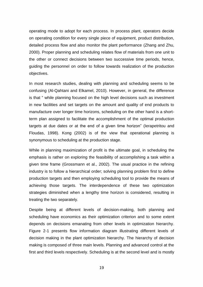
Figure 2-6: Crude oil TBP curve with swing cuts (Alattas et al., 2011) ............. 28

Figure 2-7: CDU representations for the FI model (Alattas et al., 2011) ........... 28

Figure 2-8: Process schematic of a typical refinery VDU (Ronald and Colwell, 2010) ......................................................................................................... 29

Figure 2-9: Process schematic of a typical refinery NHU (Ronald and Colwell, 2010) ......................................................................................................... 30

Figure 2-10: Process schematic of a typical refinery FCC (Ronald and Colwell, 2010) ......................................................................................................... 31

Figure 2-11: Process schematic of a typical refinery CRU (Ronald and Colwell, 2010) ......................................................................................................... 33

Figure 3-1: Flow network diagram for Case 1 (Lee et al., 1996)....................... 56

Figure 3-2: Optimal schedule for Case 1 .......................................................... 58

Figure 3-3: Optimal volume variations in storage tanks .................................... 59

Figure 3-4: Optimal volume variations in charging tanks .................................. 60

Figure 3-5: Optimal CDU charging schedule .................................................... 61

Figure 3-6: Optimal variation in concentration of sulphur ................................. 62

Figure 3-7: Comparison of optimal schedule for Cases 1 and 2 ....................... 63

Figure 3-8: Optimal volume variations in storage tanks for Case 1 and Case 2 64

Figure 3-9: Optimal volume variations in charging tanks for Case 1 and Case 2 .................................................................................................................. 65

Figure 3-10: Optimal tank-tank schedule .......................................................... 68

Figure 3-11: Optimal schedule (with set up cost) for Case 3 ............................ 69

Figure 3-12: Optimal volume variations in storage tanks .................................. 70

x

Figure 3-13: Optimal volume variations in charging tanks ................................ 70

Figure 3-14: Optimal CDU schedules for Scenario C ....................................... 73

Figure 4-1: Fixed end receding horizon ............................................................ 76

Figure 4-2: Moving end receding horizon ......................................................... 77

Figure 4-3: Optimal schedule for Case 1 .......................................................... 79

Figure 4-4: Optimal schedule for time step 2 .................................................... 79






Figure 4-10: Storage tanks inventory levels for normal simulation and fixed end horizon strategy ......................................................................................... 82

Figure 4-11: Charging tanks inventory levels for normal simulation and fixed end horizon strategy ......................................................................................... 82

Figure 4-12: CDU charging schedule ............................................................... 84

Figure 4-13: Storage tanks inventory levels for nominal simulation, fixed end and moving end horizon strategies ............................................................ 84

Figure 4-14: Charging tanks inventory levels for nominal simulation, fixed end and moving end horizon strategies ............................................................ 85

Figure 5-1: Discrete and Continuous time representations (Floudas and Lin, 2004) ......................................................................................................... 88

Figure 5-2: Refinery production with product blending(Alattas et al., 2011) ... 100

Figure 6-1: Production levels for SR fuel gas at different time periods ........... 120

Figure 6-2: Production levels for SR gasoline at different time periods .......... 121

Figure 6-3: Production levels for SR naphtha at different time periods .......... 121

Figure 6-4: Production levels for SR distillate at different time periods .......... 121

Figure 6-5: Production levels for SR gas oil at different time periods ............. 122

Figure 6-6: Production levels for SR residuum at different time periods ......... 122

xi

LIST OF TABLES

Table 3-1: System information for Case 1 (Yüzgeç et al., 2010) ...................... 57

Table 3-2: Comparison between optimal cost for Cases 1 and 2 ..................... 63

Table 3-3: System information for Case 3 (Lee et al., 1996) ............................ 67

Table 3-4: Scenario A data ............................................................................... 71

Table 3-5: Scenario B data ............................................................................... 72

Table 4-1: System information for Case 1 ........................................................ 78

Table 4-2: System information for Case 2 ........................................................ 83

Table 5-1: Crude cuts IBP and EBP ............................................................... 101

Table 5-2: Crude assay data .......................................................................... 101

Table 5-3: Crude oil availability (1000s bbl/day) ............................................. 102

Table 5-4: Refinery raw material/operating costs and product prices ............. 102

Table 5-5: Yield patterns for the downstream process units ........................... 103

Table 5-6: Capacities of process units (1000 bbl/day) .................................... 103

Table 5-7: Blending information from yields ................................................... 103

Table 5-8: Product quality specifications ........................................................ 104

Table 5-9: minimum run length for each blending operation (per day) ........... 104

Table 5-10: Demand of final products (1000s bbl per day) ............................. 104

Table 5-11: Bounds on amount produced and tank inventory (1000s) ........... 105

Table 5-12: Income and costs generated for the whole scheduling horizon ($1000) .................................................................................................... 105

Table 5-13: Raw material processing information .......................................... 106

Table 5-14: Product sales .............................................................................. 106

Table 5-15: Product inventory levels .............................................................. 107

Table 5-16: Income and costs generated for the whole scheduling horizon ($1000) .................................................................................................... 108

Table 5-17: Raw material processing information .......................................... 108

Table 6-1: Parameter values from regression ................................................ 119

Table A-1: Initial micro-cuts distribution into their respective cuts for Crude 1 143

Table B-1: Initial micro-cuts distribution into their respective cuts for Crude 2 145

xiii

LIST OF EQUATIONS

(2-1) .................................................................................................................. 11

(2-2) .................................................................................................................. 12

(2-3) .................................................................................................................. 13

(2-4) .................................................................................................................. 15

(3-1) .................................................................................................................. 44

(3-2) .................................................................................................................. 45

(3-3) .................................................................................................................. 45

(3-4) .................................................................................................................. 45

(3-5) .................................................................................................................. 45

(3-6) .................................................................................................................. 46

(3-7) .................................................................................................................. 46

(3-8) .................................................................................................................. 46

(3-9) .................................................................................................................. 46

(3-10) ................................................................................................................ 46

(3-11) ................................................................................................................ 46

(3-12) ................................................................................................................ 47

(3-13) ................................................................................................................ 47

(3-14) ................................................................................................................ 47

(3-15) ................................................................................................................ 48

(3-16) ................................................................................................................ 48

(3-17) ................................................................................................................ 48

(3-18) ................................................................................................................ 49

(3-19) ................................................................................................................ 49

(3-20) ................................................................................................................ 49

(3-21) ................................................................................................................ 49

(3-22) ................................................................................................................ 49

(3-23) ................................................................................................................ 50

(3-24) ................................................................................................................ 50

xiv

(3-25) ................................................................................................................ 51

(3-26) ................................................................................................................ 51

(3-27) ................................................................................................................ 51

(3-28) ................................................................................................................ 51

(3-29) ................................................................................................................ 52

(3-30) ................................................................................................................ 52

(3-31) ................................................................................................................ 52

(3-32) ................................................................................................................ 52

(3-33) ................................................................................................................ 52

(3-34) ................................................................................................................ 53

(3-35) ................................................................................................................ 53

(3-36) ................................................................................................................ 53

(3-37) ................................................................................................................ 53

(3-38) ................................................................................................................ 54

(3-39) ................................................................................................................ 54

(3-40) ................................................................................................................ 54

(3-41) ................................................................................................................ 54

(3-42) ................................................................................................................ 55

(3-43) ................................................................................................................ 55

(3-44) ................................................................................................................ 55

(3-45) ................................................................................................................ 55

(5-1) .................................................................................................................. 92

(5-2) .................................................................................................................. 92

(5-3) .................................................................................................................. 92

(5-4) .................................................................................................................. 93

(5-5) .................................................................................................................. 93

(5-6) .................................................................................................................. 93

(5-7) .................................................................................................................. 93

(5-8) .................................................................................................................. 93

xv

(5-9) .................................................................................................................. 94

(5-10) ................................................................................................................ 94

(5-11) ................................................................................................................ 94

(5-12) ................................................................................................................ 94

(5-13) ................................................................................................................ 94

(5-14) ................................................................................................................ 94

(5-15) ................................................................................................................ 95

(5-16) ................................................................................................................ 95

(5-17) ................................................................................................................ 95

(5-18) ................................................................................................................ 95

(5-19) ................................................................................................................ 95

(5-20) ................................................................................................................ 96

(5-21) ................................................................................................................ 96

(5-22) ................................................................................................................ 96

(5-23) ................................................................................................................ 96

(5-24) ................................................................................................................ 96

(5-25) ................................................................................................................ 97

(5-26) ................................................................................................................ 97

(5-27) ................................................................................................................ 97

(5-28) ................................................................................................................ 97

(5-29) ................................................................................................................ 97

(5-30) ................................................................................................................ 97

(5-31) ................................................................................................................ 97

(5-32) ................................................................................................................ 97

(5-33) ................................................................................................................ 98

(5-34) ................................................................................................................ 98

(5-35) ................................................................................................................ 98

(5-36) ................................................................................................................ 98

(5-37) ................................................................................................................ 98

xvi

(5-38) ................................................................................................................ 98

(5-39) ................................................................................................................ 98

(5-40) ................................................................................................................ 99

(5-41) ................................................................................................................ 99

(6-1) ................................................................................................................ 113

(6-2) ................................................................................................................ 114

(6-3) ................................................................................................................ 114

(6-4) ................................................................................................................ 115

(6-5) ................................................................................................................ 115

(6-6) ................................................................................................................ 115

(6-7) ................................................................................................................ 116

(6-8) ................................................................................................................ 116

(6-9) ................................................................................................................ 117

(6-10) .............................................................................................................. 117

(6-11) .............................................................................................................. 117

(6-12) .............................................................................................................. 117

(6-13) .............................................................................................................. 117

(6-14) .............................................................................................................. 118

(6-15) .............................................................................................................. 118

(6-16) .............................................................................................................. 118

(6-17) .............................................................................................................. 119

xvii

LIST OF ABBREVIATIONS

BB Branch and Bound

bbl Barrels

bpsd Barrels per stream day

AGO Automotive Gas Oil

ANN Artificial Neural Network

API American Petroleum Institute

ASTM American Society for Testing Materials

CCR Continuous Catalyst Regeneration Unit

CDU Crude Distillation Unit

CDUs Crude Distillation Units

CRU Catalytic Reforming Unit

CT Charging Tank

CV Control Variable

DICOPT Discrete and Continuous Optimizer

EBP End Boiling Point

ETBE Ethyl Tertiary Butyl Ether

FCC Fluid Catalytic Cracking Unit

FI Fractionation Index

GAMS General Algebraic Modelling Systems

GB Gasoline Blending

GBD Generalized Benders Decomposition

GUI Graphical User Interface

HDS Hydro-desulphurisation

HVGO Heavy Vacuum Gas Oil

IBP Initial Boiling Point

KHU Kero Hydrotreating Unit

KKT Karush Kun Tucker

KRPC Kaduna Refining and Petrochemical Company

LHS Left Hand Side

LP Linear Programming

LPG Liquified Petroleum Gas

LVGO Light Vacuum Gas Oil

xviii

MILP Mixed Integer Linear Programming

MINLP Mixed Integer Nonlinear Programming

MPC Model Predictive Control

MTBE Methyl Tertiary Butyl Ether

NCO Necessary Condition of Optimality

NHU Naphtha Hydrotreating Unit

NLP Nonlinear Programming

PC Personal Computer

PID Proportional Integral Derivative

PTDF Petroleum Technology Development Fund

RHS Right Hand Side

SOC Self-Optimizing Control

SR Straight Run

SSE Sum of Square Error

ST Storage Tank

STN State Task Network

TAME Tertiary Amyl Methyl Ether

TBP True Boiling Point

TBR Trickle bed Reactor

TGO Total Gas Oil

ULSD Ultra-low Sulphur Diesel

VDU Vacuum Distillation Unit

VO Vacuum Overhead

VR Vacuum Residue

WRPC Warri Refining and Petrochemical Company

1

1 INTRODUCTION

1.1 Background

In recent years the downstream sector of the petroleum industry faces great

challenges to survive competition, improve profit margin, and to operate within

the boundaries of the environmental legislations (Li et al., 2012b). Despite these

issues, petroleum refiners operate while taking into consideration the

uncertainty associated with rise and fall in product demands, unavoidable

change in crude oil prices, fluctuation in quality and composition of feed

material, lead time, and quality of gasoline and diesel produced. This

necessitates exploring viable alternatives to compete successfully and remain in

business (Li et al., 2012a).

The current practice in the industry is that refiners resort to devising reliable and

the most cost effective and feasible operational procedures to address both

economic and environmental issues that have significant impacts on the refining

business through planning and scheduling. From Karuppiah et al. (2008),

planning and scheduling of refining operations are necessary as benefits in

terms of production cost savings and feed improvement are potentially realized.

According to Fagundez and Faco (2007), planning and scheduling allow

optimum utilization of resources; ensure availability of high quality products and

guarantee a positive return on investment.

While planning is forecast driven, scheduling on the other hand, is order driven;

making use of available resources and time to model and solve refinery

operational problems. Planning always precedes scheduling and the planning

decisions are generated for implementation during scheduling; implying that

good scheduling is a direct consequence of good planning (Kelly and Mann,

2003a). Integrating the two will improve efficiency and reliability of the refinery

decision making processes, though it is still a challenge. Moreover,

consideration to uncertainty offers robustness and flexibility.

2

1.2 Configuration of an oil refinery

An oil refinery processed crude oil of varying compositions into useful petroleum

products while utilizing various economic and environmental alternatives (Gary

and Handwerk, 1984). Its configuration varies from one refinery to another

depending on the products demand and quality requirements of available

customers. For example, some refineries in Nigeria like Kaduna Refining and

Petrochemical Company (KRPC), and Warri Refining and Petrochemical

Company (WRPC) were designed to produce petrochemicals in addition to the

conventional fuel products.

Petroleum refineries differ in the plant configurations. Despite the differences,

however most process units are common. They are: crude distillation unit

(CDU), vacuum distillation unit (VDU), fluid catalytic cracking unit (FCC),

naphtha hydrotreating unit (NHU), catalytic reforming unit (CRU) and gas

treating unit. Alkylation and Isomerization process units are also part of refinery

production plant.

In general, most refineries, in addition to the processing units mentioned in the

preceding paragraph, have one or more units and this varies depending on the

design that suits the refiners plan. Figure 1-1 is a process flow diagram of a

typical oil refinery plant showing most of the unit processes, with stream

connections from crude oil feed to the final products. Other refinery

configurations may have more or less of the units presented here. For example,

utility section and blending units are not shown in Figure 1-1.

Also of importance in other refinery configurations are the use of butane or

oxygenated compounds (oxygenates) as additive materials in blending units.

The materials are added to improve octane rating of the final products.

Oxygenates are ether compounds derived from their respective alcohols. They

include: Methyl tertiary butyl ether (MTBE), Ethyl tertiary butyl ether (ETBE) and

Tertiary amyl methyl ether (TAME). Of these three oxygenates, MTBE is the

most acceptable in gasoline blending, meeting all the gasoline pool objectives.

This compound has the blending quality of 109 octanes, a RVP blending of 8–

10 psi and a boiling point of 131◦F (Jones and Pujado, 2006).

3

Figure 1-1: A process flow diagram of an oil refinery plant (Anon, 2011)

1.3 Motivation

Traditionally, petroleum refinery operations are based on heuristic rules. The

recent advancements in modern computing provide opportunities for

automation, hence systematic approaches are always devised to generate

guidelines and operational procedures that guarantee smooth conduct of

refining business at minimal cost. While mathematical techniques for refinery

planning have a long established popularity in petroleum research studies,

much less has been reported in scheduling of production area, and to some

extent in crude oil scheduling. Models developed previously have shortcomings

in one way or the other that practical implementation of decisions obtained from

4

solving the models may fail to reflect realities. Some of these modelling issues

have been addressed in this work.

Generally, crude oil refinery operates under economic and environmental

conditions bounded with uncertainties. According to Mula et al. (2006), models

which do not take into cognizance a number of uncertainties can be expected to

generate unreliable decisions when compared to models that explicitly or

implicitly incorporate those uncertainties. In most of the work reported in refinery

planning and scheduling, uncertainties from design point of view predominate.

However, there is also a need to consider operational uncertainties as they

affect the accuracy and robustness of the overall schedule. This challenge has

been taken care of in this study.

Developing methodologies and solution algorithms for scheduling of refinery

systems with uncertainty considerations is therefore imperative. Obtaining

accurate and reliable schedules for crude oil unloading, refining and blending of

final products within the scheduling cycle is the motivation behind this work. A

variety of modelling and solution options are developed to match peculiarities of

problems in different refinery subsystems with decisions to be implemented in a

real plant.

1.4 Novelty

In process design, uncertainties are considered in order to generate robust

schedules in anticipation of unforeseen circumstances. However, operational

uncertainties in the form of disturbances do manifest during schedule execution

in the real plant and therefore more efficient techniques have to be developed

and applied in the schedule generation. Therefore this study will propose novel

approaches to model and deal with uncertainty as disturbance in refinery

scheduling operation. To achieve the objectives of this research, a number of

contributions have been made to scientific body of knowledge in this area of

study.

Firstly, an existing mixed integer linear programming (MILP) model by Lee et al.

(1996), which was formulated to minimise operational cost associated with

5

crude oil unloading, processing and inventory control, has been extended to

make the model reflects real industrial applications. In this work, the model was

extended by including important technical details to adequately capture real

industrial practices in crude oil scheduling (Hamisu et al., 2013a; Hamisu et al.,

2013b).

Among other things, the extended model accounts for interval-interval charging

rate fluctuations in CDU, demand violation against obtaining infeasible solution

and adopt more realistic operational procedures (Hamisu et al., 2013a; Hamisu

et al., 2013b). The extended model was assessed relative to the existing model

to highlight the benefits derived in terms of performance. Also, some scenarios

were created to make recommendations to the refinery operators in deciding

the best schedule to use.

The model was then used to demonstrate the capability of fixed end horizon

control strategy to accommodate CDU demand uncertainty within the

scheduling horizon. The result was then compared with another control strategy

of model predictive control (moving end horizon control) for scheduling crude oil

unloading presented in Yüzgeç et al. (2010). The approach proposed in this

work is more realistic considering that plant operators work with schedules for a

specified period of time with fixed deadline and have more degrees of freedom

in accommodating uncertainties since the solution search covers the whole

scheduling horizon.

A mixed integer nonlinear programming formulation for simultaneous

optimization of production scheduling with product blending was developed to

include blending units in addition to other units commonly found in oil refinery.

The model considers crude oil characteristics with pseudo-components

generated from ASPEN plus for two different crude oil grades. In addition to

flow rates, crude compositions are also considered. The CDU model is based

on swing cut approach and the objective of the optimization model is to

maximize profit while generating feasible schedules within time horizon.

A data driven self-optimizing control (SOC) strategy was developed to deal with

multi-period scheduling problems under uncertain conditions. The goal was to

6

achieve global optimum by maintaining the gradient of the cost function at zero

via approximating necessary conditions of optimality (NCO) over the whole

uncertain parameter space. A regression model for the plant expected revenue

(profit) as a function of independent variables using optimal operation data was

obtained and a feedback input (manipulated variable) was derived. Data for

regression was generated from the mixed integer nonlinear programming model

discussed in the preceding paragraph.

1.5 Aims and Objectives

The aim of this study is to develop robust methodologies and solution

procedures to address refinery scheduling problems under uncertain conditions.

The main objectives are:

To develop a mixed integer linear programming formulation for short-

term crude oil unloading, tank inventory management, and CDU charging

schedule as an extension to a previous work reported by Lee et al.

(1996).

To investigate the performance of the extended model through case

studies and create scenarios to generate schedules under disruptive

event and low inventory at the end of scheduling horizon.

To devise a solution alternative to deal with uncertainty in crude oil

scheduling via model predictive control strategy.

To develop a mixed integer nonlinear programming formulation for

simultaneous optimization of production scheduling with product

blending.

To develop a data driven SOC strategy for multi-periods scheduling

problems.

To apply the SOC strategy to solve discrete time mixed integer nonlinear

programming model for production scheduling with product blending.

Disturbance scenarios (uncertainties in crude oil compositions) will be

introduced to test the efficacy of the SOC method.

7

1.6 Outline of Thesis

Chapter 2 focuses on the literature review for refinery scheduling with

discussion on the techniques available in literature to address uncertainties.

Modelling of refinery subsystems and current and future direction in this

research area will be discussed.

Chapter 3 discusses modelling crude oil unloading area where benefits of our

formulation (extended MILP model) for crude oil unloading scheduling with tank

inventory management were highlighted.

Chapter 4 presents receding horizon approaches to handle problems in crude

oil scheduling, blending, and tanks inventory management under CDU demand

uncertainties. Comparison between fixed-end and moving-end strategies in

terms of performance was discussed.

In Chapter 5, a novel mixed integer nonlinear formulation for short-term

scheduling of refinery production with product blending will be covered.

Chapter 6 covers multi-period data driven SOC strategy to address

uncertainties in a large-scale refinery production scheduling problem.

Finally, conclusions and recommendations are presented in Chapter 7.

1.7 Publications and Conferences

Journal paper

Hamisu, A. A., Kabantiok, S., & Wang, M.; Refinery Scheduling of Crude oil

Unloading with Tank Inventory Management; Computers and Chemical

Engineering 55, (2013) 134-147.

Conferences

Hamisu, A. A., Kabantiok, S., & Wang, M.; “An improved MILP model for

scheduling crude oil unloading, storage and processing” pp. 631-636. 23rd

European Symposium on Computer Aided Process Engineering, ESCAPE23

held in Lappeenranta, Finland on 9-12/06/2013.

8

Hamisu, A. A., Cao, Y., & Kokossis, A.; “Scheduling crude oil blending and

tanks inventory control under CDU demand uncertainty: A receding horizon

approach” pp. 260-265. 20th International Conference on Automation and

Computing, ICAC14 held at Cranfield University, Bedfordshire, UK on 12-

13/09/2014.

Papers in preparation (Journal)

Hamisu, A. A., Cao, Y., & Kokossis, A.; Receding horizon approach for

scheduling crude oil blending and tanks inventory management

Hamisu, A. A., Cao, Y., & Kokossis, A.; Refinery production scheduling under

self-optimizing control framework

9

2 LITERATURE REVIEW

In a petroleum refinery, optimization is performed at three levels of decision,

namely; planning, scheduling and control. The relationship between the three

levels is such that planning set targets while scheduling executes the target to

provide optimal values of decision variables as set points for controllers.

Moreover, control actions through feedback mechanisms can be applied to

address scheduling problems with uncertainty in process parameters.

Integrating these levels in a complex plant like refinery is virtually impossible.

However, at most a combination of two levels can be handled together when

the refinery plant is decomposed into subsystems (crude oil unloading area,

production area and product blending area) and treat the subsystems

separately.

This chapter presents literature review on refinery scheduling with

considerations on techniques and algorithmic procedures used to deal with

problems under uncertain conditions. The review will discuss formulation of

optimization problems as linear programming (LP), nonlinear programming

(NLP), mixed integer linear programming (MILP), and mixed integer nonlinear

programming (MINLP). Modelling and simulation tools used in this research

work will then be discussed. Subsequent paragraphs in this chapter will be on

the relationship between planning and scheduling, then broad areas of

petroleum refinery including process units for scheduling, consideration for

uncertainties and, the current and future trend in refinery scheduling.

2.1 Refinery Optimization Problems

Edgar et al. (2001) defined optimization as ‘’the use of specific methods to

determine the most cost-effective and efficient solution to a problem or design

for a process’’. It is concerned with selecting the best among many solution

alternatives using efficient quantitative methods. Optimization aims at finding

the values of decision variables in process that yield the best value of

performance criterion. Optimization problem formulation consists of the

following components:

10

Objective function

Constraints

Decision variable(s) and

Parameters

The objective function is usually a mathematical expression relating decision

variables with coefficients called parameters. Constraints on the other hand

relate decision variables with coefficients and right hand side (RHS) values. The

constraints can be equality or inequality. When formulated mathematically,

optimization problems potentially involve many of the components mentioned

above. In relation to obtaining solution of optimization problem, three important

concepts are defined:

Feasible region: is the region of feasible solutions.

Feasible solution: are set of variables that satisfy equality and inequality

constraints. and

Optimal solution: a feasible solution that provides the optimal value of the

objective function.

From these definitions, an optimal solution must not only achieve an extremum

of the objective function, such as minimizing cost or maximizing profit but also

must satisfy all of the constraints (Edgar et al., 2001).

Depending on the nature of the objective function and constraints, optimization

problem can be LP, NLP, MILP or MINLP. In the past decades, optimization

problems are solved using manual calculations at very high computational cost

and with no guarantee to obtain accurate results. This was later improved

slightly with the availability of spreadsheet packages, though less rigorous

compared to the manual computational approach. The recent advancement in

computing coupled with the availability of software programmes makes it easier

to solve optimization problems within reasonable time frame. The algorithm

embedded in the software programmes depends on the nature of the

optimization problem required to solve.

11

2.1.1 LP

LP is a class of optimization problem in which both the objective function and

constraints are linear. LP is the most widely encountered optimization problem

in manufacturing and processing industries, which constitutes number of

variable(s) and constraints (Edgar et al., 2001). As an example, LP problem can

be formulated as,

Minimize: 𝑓 = 𝑥1 + 2𝑥2 − 5𝑥3

Subject to: − 2𝑥2 + 𝑥3 ≤ 8

𝑥1 + 𝑥3 = −4

𝑥1, 𝑥2, 𝑥3 ≥ 0

(2-1)

In Equation 2-1, the objective function 𝑓 is to be minimized. The objective

function has no products of two variables (bilinear terms) or three variables

(trilinear terms). Also in the objective function, there is no division of variables.

Variables in basic functions like trigonometric, exponential, differential and

integral are not included. Therefore the objective function is linear with respect

to the variables. The second and third mathematical relations in Equation 2-1

are inequality and equality constraints respectively. Like objective function, the

constraints are also linear based on the reasons already stated. The last

expression is called bounds forcing all the variables to be positive. For example

the bounds may be representing capacities of processing units in refinery which

can never be negative.

LP problems can be solved using a two-phase procedure called simplex

method. The first phase finds an initial basic feasible solution if a solution of the

problem exist and reports detail information for a case where no solution is

available. No solution to a problem may be due to inconsistency in constraints.

In the second phase, the solution depends on the outcome of the first phase

and the result can be positive (optimum found) or negative (unbounded

minimum). Most commercial solvers work based on this algorithm.

12

LP is usually preferred due to the ease of formulation and can be used to

approximate nonlinear model around its steady state; this reduces the

complexity and of course makes it less hectic to solve. Though, its choice is

usually a trade-off between simplicity and robustness (Floudas and Lin, 2005).

Although employed in most process systems, LP does not receive a wider

acceptance in refinery scheduling.

2.1.2 NLP

NLP is an optimization problem that seeks to minimize (or maximize) a

nonlinear objective function subject to linear or nonlinear constraints. Problems

formulated as NLP are more accurate compared to their LP counterparts since

most chemical processes are nonlinear in nature. Refinery models that account

for nonlinear relationship of process variables are more reliable and represent

the refinery systems more closely. The general representation of NLP problems

is as shown in Equation 2-2.

Minimize: 𝑓(x) x=[𝑥1 𝑥2 . . . 𝑥𝑛]𝑇

Subject to: ℎ𝑖(x) = 𝑏𝑖 𝑖 = 1, 2, . . . , 𝑚

𝑔𝑗(x) ≤ 𝑐𝑗 𝑗 = 1, . . . , 𝑟

(2-2)

In this formulation, bilinear and trilinear terms, and basic mathematical functions

can be found. In Equation 2-2, at least the objective function 𝑓(x), the equality

constraint ℎ𝑖(x) or the inequality constraint 𝑔𝑗(x) must be nonlinear.

The challenge in modelling using NLP formulation is that of achieving a

reasonable convergence. This is largely due to the fact that many real-valued

functions are non-convex. Convexity of feasible region can only be guaranteed

if constraints are all linear. Moreover, it is a difficult task to tell if an objective

function or inequality constraints are convex or not. However, convexity test can

be carried out to satisfy first-order necessary conditions of optimality popularly

known as Kuhn-Tucker conditions (also called KKT conditions). Most algorithms

embedded in commercial solvers terminate when these conditions are satisfied

within some tolerance. For problems with a few number of variables, KKT

13

solutions can sometimes be found analytically and the one with the best

objective function value is chosen. It is not within the scope of this work to

discuss KKT conditions in more detail. The reader should refer to Edgar et al.

(2001) or other related materials.

Unlike LP, NLP are reported in a significant number of publications in refinery

problems involving blending relation and pooling. Moro et al. (1998) developed

a non-linear optimization model for the entire refinery topology with all the

process units considered and non-linearity due to blending included. Their work

has been extended by Pinto et al. (2000); Neiro and Pinto (2005) for multi-

period and multi-scenario cases involving non-linear models. In this work,

nonlinearity is considered in the development of scheduling model for refinery

production with product blending.

2.1.3 MILP

This optimization problem involves discrete and continuous decisions, with

linear objective function(s) and linear constraint(s). MILP allows the discrete and

continuous features of optimization problem to be adequately represented; thus

enabling refiners to select the optimum allocation of task to processing units in

the refinery plant. A decision to use or not to use particular equipment at a

particular time period can be modelled using binary variables (0-1). The value

‘1’ means the equipment is in use and ‘0’ otherwise. Besides 0 and 1, integer

variables can be real numbers 0, 1, 2, 3, and so on. Sometimes integer

variables are treated as if they were continuous in problems where the variable

range contains large number of integers. In such a case, the optimal solution is

rounded to the nearest integer value. Generally, MILP problem is presented in

the following form:

Minimize: 𝒄𝑥𝑇 x + 𝒄𝑦

𝑇 y

Subject to: 𝐴𝐱 + 𝐵𝐲 ≤ 0

𝐱 ≥ 0

𝐲 ∈ {0,1}𝑞

(2-3)

14

The objective function here depends on two sets of variables, 𝒙 and 𝒚; 𝒙 is a

variable vector representing continuous decisions (volume, flowrates,

temperature, concentration) and 𝒚 variables represent discrete decisions. 𝐴, 𝐵

and 𝒄 are the coefficient matrices.

Like LP, MILP problems are linear in the objective function and constraints

hence the problems are readily solved by many LP solvers. MILP problems are

much harder to solve than their LP counterparts. As the number of integer

variables are becoming larger, the computational time for even the best

available MILP solvers increases rapidly. Using branch and bound (BB)

algorithm embedded in commercial solvers such as CPLEX, GUROBI, MOSEK,

SULUM, XA and XPRESS, optimal solution of MILP problems can be obtained.

BB works by generating LP relaxation of the original MILP problem, allowing the

0 or 1 constraint to be relaxed (taking value anywhere between 0 and 1). The

algorithm starts by solving the LP relaxation such that if all the discrete

variables have integer values, the solution solves the original problem otherwise

one or more discrete variables has a fractional value and the solution search

has to continue through branching. To continue with the solution search BB

chooses one of the discrete variables and creates LP subproblems by fixing this

variable at 0, then at 1. If either of the subproblem has an integer solution or

infeasible, the subproblem will not be investigated further. If the objective value

of the subproblem is better than the best value found so far, it replaces this best

value. A bounding test is then applied to each subproblem and if the test is

satisfied, the subproblem will not be investigated further otherwise branching

continues (Edgar et al., 2001).

Most of the problems reported in refinery scheduling are MILPs especially in

crude oil unloading area due to the need to consider both continuous and

discrete decisions. The model presented in the next chapter of this work was

formulated as MILP problem and solved using CPLEX solver in GAMS software

programme.

15

2.1.4 MINLP

Many process systems are best described with nonlinear models. Therefore in

addition to being mixed integer, this class of optimization problem include

nonlinearity in the objective function, or constraints or both. The general

representation of this optimization problem is:

Minimize: 𝑓(x, y)

Subject to: 𝒉(x, y) = 0

𝒈(x, y) ≤ 0

𝒙 ∈ ℝ𝑛

𝒚 ∈ {0,1}𝑞

(2-4)

MINLP are much harder to solve than LP, NLP or MILP due to the combinatorial

nature of the problem which arises from the presence of binary variables, and,

when the nonlinear functions are nonconvex; the solution converges to a local

optimum. Like MILP, MINLP can also be solved using BB with the main

difference being that the relaxation at each node is NLP rather than LP. Another

algorithm to solve MINLP problem is the Generalized Benders Decomposition

(GBD). The GBD algorithm works based on the principles of partitioning the

variable set, followed by decomposition of the problem and finally refinement is

done iteratively.

In the partitioning of the variable set, the y variables are referred to as

complicating variables and handled differently from the x variables thus

enabling the algorithm to be used to handle bilinear non-convexities in a

rigorous manner. Decomposition involves solving the problem by considering

two types of derived problems: a primal problem which provides an upper

bound on the MINLP, and a master problem which provides a lower bound on

the MINLP. Using the information obtained from any given primal and master

problems, new sets of primal and master problems are created in such a way

that the bounds become tighter and within a finite number of iterations

16

convergence can be achieved. Integer cuts may be added in order to avoid

generating any combination of the binary variables twice.

MINLP problem can also be solved using another algorithm called Outer

approximation (Duran and Grossmann, 1986; Floudas, 1995). The algorithm

which has an interface with General Algebraic Modelling Systems (GAMS) and

is implemented in a software programme called Discrete and Continuous

Optimizer (DICOPT). It works through a series of iterations in such a way that at

each major iteration, two subproblems (a continuous variable nonlinear program

and a linear mixed-integer program) are solved.

2.2 Modelling and Simulation Tools

GAMS, Aspen PLUS and Matlab are used in this study. GAMS was used for the

modelling and optimization of all MILP and MINLP formulations developed in

this work. Crude characterization to generate pseudo-components for

distribution to corresponding cut fractions was achieved using Aspen PLUS.

While the regression analysis for the data driven self-optimizing control (SOC)

was carried out in Matlab. Brief introduction of the software tools will be given.

2.2.1 GAMS

GAMS is a modelling tool developed for setting up and solving large-scale

optimization problems. It was developed to address optimization problems in

the early 1970s with the following objectives:

Providing the language base that will allow easy representation of

compact data and complex models.

Allowing changes to be made in models without difficulty.

Permitting model description that is not dependent on algorithms used to

achieve solution (Rosenthal, 2012).

The GAMS modelling language is algebraic with optional interfaces for LP, NLP,

MILP and MINLP solvers. The modelling system is available in a wide variety of

platforms ranging from personal computers (PCs) to workstations and

mainframe computers. This software programme works by accepting model

17

specifications as a system of algebraic equations, then parses the equations to

transform them into a form that can easily be evaluated numerically by its

interpreter. Before the processed model is made available to solver, some

analysis are also carried out by the modelling system to determine the model

structure (Edgar et al., 2001).

GAMS is a powerful tool used in most academic research activities as it allows

users to specify the structure of the optimization model, specify data and

calculate data fed into the model, solve the model based on the constraints

imposed and aid the comparative statistical analysis of results. Models in

Chapters 3, 4 and 5 in this work are solved using this software programme.

2.2.2 Aspen PLUS

Aspen PLUS is a simulation package providing an environment for modelling,

design, optimization, and performance monitoring of chemical processes. It has

a graphical user interface (GUI) that allows users to create and manipulate fluid

packages or component lists in the simulation environment. Using Aspen PLUS

for crude oil characterization, the user can:

Define components

Enter assay data for any number of crudes

Blend the crudes to produce feed material for distillation units

Generate pseudo-components for individual crudes and crude blends

Carry out assay data analysis

View and interprets results.

2.2.3 Matlab

Matlab is a high-performance language for technical computing. It integrates

computation, visualization, and programming environment. Matlab was

developed as an interactive program for doing matrix calculations and has now

grown to a high level mathematical language that can solve integral and

differential equations numerically and plot a wide variety of two and three

dimensional graphs (O'Connor, 2012). It has sophisticated data structures,

contains built-in editing and debugging tools, and supports object-oriented

18

programming. These factors make Matlab an excellent tool for teaching and

research.

The recent work of Ferris et al. (2011) provides a means by which GAMS and

Matlab can interface. GDXMRW utilities in GAMS allow data to be

imported/exported between GAMS and Matlab and to call GAMS models from

Matlab and get results back in Matlab. The software gives Matlab users the

ability to use all the optimization capabilities of GAMS, and allows visualization

of GAMS models directly within Matlab.

2.3 Planning and Scheduling

In oil and gas industries, decisions have to be taken to operate plants at

minimum cost in order to improve the overall profit margin. In refineries, such

decisions include selection of suitable raw materials to process, identification of

unit equipment to use, specification of the sequence of operations, and

matching amounts to be produced with the product demand from customers.

Considering the complexity of refinery operations, optimization tools are

employed to generate the most effective, reliable and robust procedures in

decision making processes.

Planning and scheduling procedure has been the subject many researchers find

a great deal of opportunity to contribute towards addressing refinery myriad

optimization problems. According to Grossmann et al. (2002), planning and

scheduling refer to a systematic way of sequencing a task and allocating the

task to equipment and personnel overtime in such a way that production targets

are met while ensuring compliance with industry operational standards.

Planning sets targets for implementation at scheduling level. In a crude oil

refinery, planning and scheduling help improve profit margin and reduce losses

arising from instability caused by wide variations of crude-charge qualities

(Ishuzika et al., 2007).

At managerial level, managers are tasked with the responsibility to decide on

the crude oil type to source for, the items to produce, the operating route to use,

the selection of catalytic material to speed up chemical reactions and the best

19

operating mode to adopt for each process. In process plant, operators decide

on operating condition for every single piece of equipment, product distribution,

detailed process flow and also monitor the plant performance (Zhang and Zhu,

2000). Proper planning and scheduling relates flow of materials from one unit to

the other or connect decisions between two successive time periods, hence,

guiding the personnel on order to follow towards realization of the production

objectives.

In most research studies, dealing with planning and scheduling seems to be

confusing (Al-Qahtani and Elkamel, 2010). However, in general, the difference

is that “ while planning focused on the high level decisions such as investment

in new facilities and set targets on the amount and quality of end products to

manufacture over longer time horizons, scheduling on the other hand is a short-

term plan assigned to facilitate the accomplishment of the optimal production

targets at due dates or at the end of a given time horizon” (Ierapetritou and

Floudas, 1998). Kong (2002) is of the view that operational planning is

synonymous to scheduling at the production stage.

While in planning maximization of profit is the ultimate goal, in scheduling the

emphasis is rather on exploring the feasibility of accomplishing a task within a

given time frame (Grossmann et al., 2002). The usual practice in the refining

industry is to follow a hierarchical order; solving planning problem first to define

production targets and then employing scheduling tool to provide the means of

achieving those targets. The interdependence of these two optimization

strategies diminished when a lengthy time horizon is considered, resulting in

treating the two separately.

Despite being at different levels of decision-making, both planning and

scheduling have economics as their optimization criterion and to some extent

depends on decisions emanating from other levels in optimization hierarchy.

Figure 2-1 presents flow information diagram illustrating different levels of

decision making in the plant optimization hierarchy. The hierarchy of decision

making is composed of three main levels. Planning and advanced control at the

first and third levels respectively. Scheduling is at the second level and is mostly

20

considered at lower corporate level (Zhang, 2006). The optimal values of

decision variables in scheduling provide the set points for controllers.

Figure 2-1: Hierarchy in decision making

2.4 Scheduling for Refinery Subsystems

The review here covers the crude oil unloading area, production area and

product blending area. It is through crude unloading area refinery receives raw

material (crude oil) for transfer to downstream units for processing. The

production area transforms crude oil into intermediate products and the

products are then sent to blending units for further processing. Review of

different work for units of the refinery subsystems/areas will be discussed in the

following sub-sections.

2.4.1 Crude Oil Unloading Area

Crude oil scheduling is a crucial part of the refinery supply chain (Saharidis et

al., 2009). It is a process that involves specifying the timing and sequence of

operations in this order of vessel arrival, crude oil unloading to storage tanks,

transferring crude oil parcels from storage tanks to charging tanks and finally

sending the mixed crude oil to Crude Distillation Units (CDUs) for component

separations and downstream processing. A typical schedule sets daily targets

21

for production with consideration on storage and charging tanks’ capacities,

CDU capacity utilization and pumping capabilities. It also determines the quality

and quantity of crude mixing materials in the charging tanks in order to produce

blends that satisfy the requirements of planning team. Each of these activities is

associated with cost. The objective of scheduling is to minimize the total cost

while following the feasible operational procedures (Jia et al., 2003).

Crude oil unloading area provides the platform for supplying the raw material to

be processed in the refinery plant. It has the facility for receiving crude oil

material and transfer the bulk quantity to the refinery plant for processing via

pipeline, large tankers and sometimes, by railroad (Guyonnet et al., 2009). In

the refinery plant, care is always taken not to degrade more expensive crude

with cheaper and low grade crude oil material by carrying out an unloading

process such that different grades are transferred into different tanks.

Segregating the different crude materials offers a greater degree of freedom to

the refiners in preparing blend recipes.

It is an operational policy that while storage tank is receiving crude oil from

vessel, it cannot feed charging tank at the same time. This will enable tank level

differences to be checked (Kelly and Mann, 2003b). Removal of brine is

normally done on receipt of crude parcel before transfer from storage to

charging tanks. Blending of crude oil is carried out in charging tanks to prepare

blends according to the CDUs demand and adequately supplied to meet

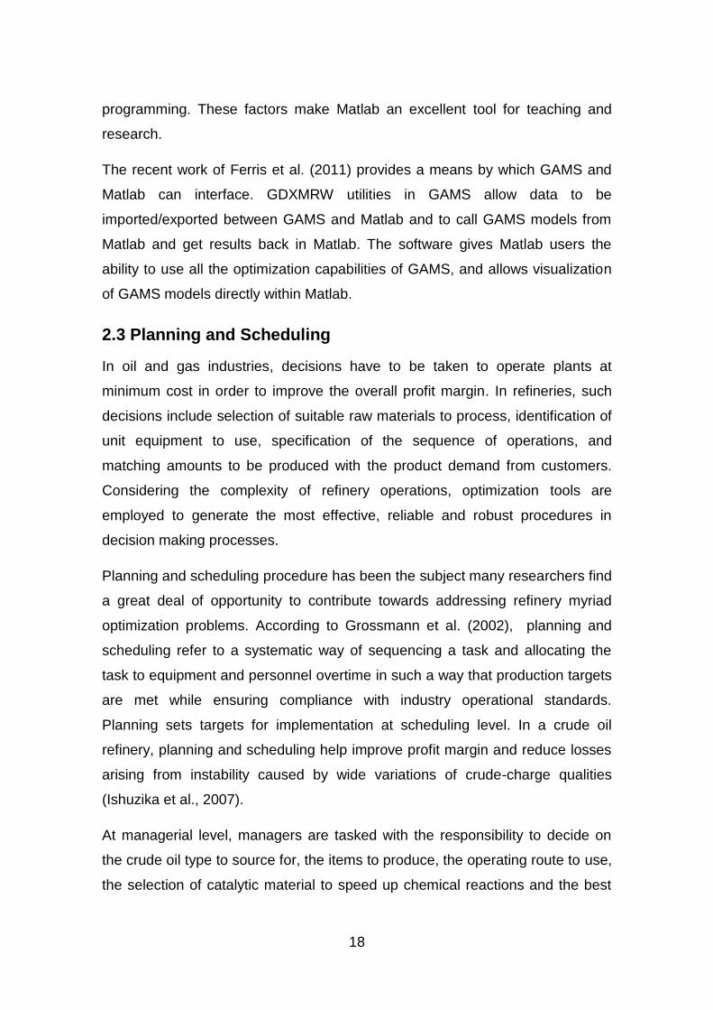
downstream processing units’ specifications. Figure 2-2 is the schematic

showing the components of the crude oil unloading area.

Research focus in crude oil unloading area has been primarily on modelling to

generate reliable schedules that reflect the ever changing dynamic environment

under which petroleum refineries operate. Since scheduling of crude oil

operations usually involves continuous and discrete decisions, MILP or MINLP

are used in formulating the scheduling problems. One of the most important

methodology developed is the work of Lee et al. (1996) that addresses the

problem of inventory management of a refinery that receives different crude

parcels within fixed scheduling horizon. Bassett et al. (1996) considers a model

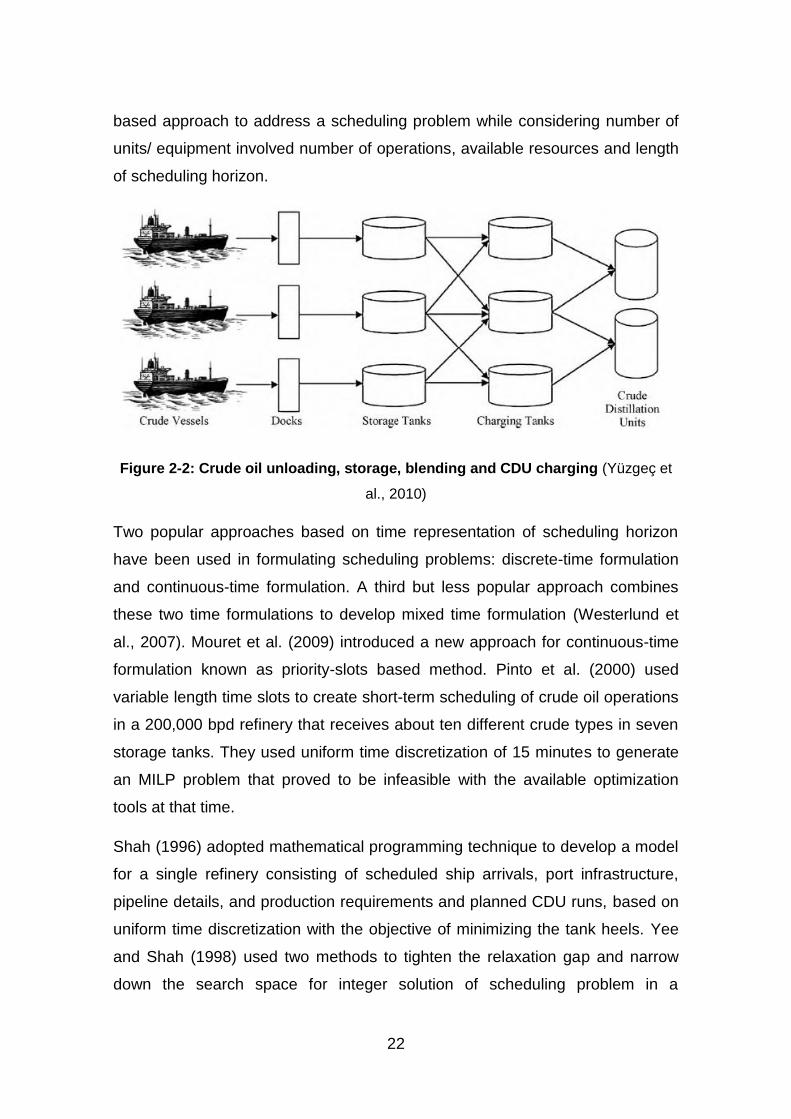
22

based approach to address a scheduling problem while considering number of

units/ equipment involved number of operations, available resources and length

of scheduling horizon.

Figure 2-2: Crude oil unloading, storage, blending and CDU charging (Yüzgeç et

al., 2010)

Two popular approaches based on time representation of scheduling horizon

have been used in formulating scheduling problems: discrete-time formulation

and continuous-time formulation. A third but less popular approach combines

these two time formulations to develop mixed time formulation (Westerlund et

al., 2007). Mouret et al. (2009) introduced a new approach for continuous-time

formulation known as priority-slots based method. Pinto et al. (2000) used

variable length time slots to create short-term scheduling of crude oil operations

in a 200,000 bpd refinery that receives about ten different crude types in seven

storage tanks. They used uniform time discretization of 15 minutes to generate

an MILP problem that proved to be infeasible with the available optimization

tools at that time.

Shah (1996) adopted mathematical programming technique to develop a model

for a single refinery consisting of scheduled ship arrivals, port infrastructure,

pipeline details, and production requirements and planned CDU runs, based on

uniform time discretization with the objective of minimizing the tank heels. Yee

and Shah (1998) used two methods to tighten the relaxation gap and narrow

down the search space for integer solution of scheduling problem in a

23

multipurpose plant. The use of time discretization presents some challenges

making other researchers to seek for more possible options such as event-

based formulations.

Saharidis et al. (2009) presented MILP formulation with uniform discrete-time

intervals where the intervals are based on events instead of hours. Jia et al.

(2003) developed a model for scheduling of oil refinery operations based on unit

specific event point formulation using the state task network (STN)

representation introduced by Kondili et al. (1993). Moro and Pinto (2004)

developed a global event-based continuous-time model for crude oil inventory

management of a refinery which processes several types of crude oil. Saharidis

et al. (2009) used an event-based time formulation for scheduling of crude oil

unloading, storage and charging of CDUs. The goal of their model was to

optimize crude oil blending and cut down the number of tank setup during

vessel unloading thereby reducing the number of tanks used.

Simplification of a complex case to problems of manageable size is an incentive

in refinery scheduling. Several authors have adopted an approach that breaks

down large scheduling problems into smaller problems. Harjunkoski and

Grossmann (2001) used a spatial decomposition strategy to split large

scheduling problem for steel production into smaller programmes. This method

produced solution within 1-3% of the global optimum. Shah et al. (2009)

presented a general novel decomposition scheme which breaks down the

refinery scheduling problem spatially into subsystems. The subsystems were

solved to optimality and the optimal results were integrated to obtain the optimal

solution for the entire problem. This results in fewer continuous and binary

variables compared to centralized systems.

2.4.2 Refinery Plant Production Area

This covers the mainstream operation of the refinery. In the production area, we

find most of the process units accomplishing the unit operations that make up

the crude oil processing. Review will be given on modelling of CDU, VDU, NHU

and FCC units. Rigorous and simplified models are discussed in the units’

modelling.

24

2.4.2.1 CDU Modelling

CDUs are the first major processing units in the refinery. They receive crude oil

from charging tanks and separate the components of the hydrocarbon material

on the basis of differences in boiling point through a separation technique called

distillation. The processing units following CDU will have feed stocks that meet

their particular specifications (Watkins, 1979). Figure 2-3 is the process

schematic of a typical CDU with auxiliary facilities (Ronald and Colwell, 2010).

Figure 2-3: Process schematic of refinery CDU (Ronald, and Colwell 2010)

In CDU modelling, yield of cut fractions are obtained from simulation of rigorous

or empirical models. Rigorous models simulate a CDU as a general distillation

column, using thermodynamic properties, energy and material balances and

equilibrium relations along the whole column to generate flow rates,

composition of internal and external streams and process conditions as outputs.

Empirical models, on the other hand, use empirical correlations to establish

material and energy balances for CDU (Li et al., 2005).

The crude assay is characterized to facilitate the computation of the CDU

yields; thus CDU is modelled in a way similar to any multicomponent, multistage

distillation column (Kumar et al., 2001). This requires at least the following

information.

25

Whole crude True Boiling Point (TBP) curve

Whole crude American Petroleum Institute (API) gravity and

Whole crude light ends analysis (Watkins, 1979).

TBP curve is presented in Figure 2-4 as a plot of TBP temperature versus

volume percent vaporized, which along with the specific gravity of crude oil

characterize the feed material (Basak et al., 2002). With the TBP curve, the

component distribution of material being tested can be analyzed in accordance

with the laid down procedures developed by the American Society for Testing

Materials (ASTM). TBP distillations are normally run only on crude oils and not

on petroleum fractions (Watkins, 1979).

American Petroleum Institute (API) gravity is defined as a ‘‘specific gravity scale

measuring the relative density of various petroleum liquids, expressed in

degrees. It is an arbitrary scale expressing the gravity or density of liquid

petroleum products devised jointly by the American Petroleum Institute and the

National Bureau of Standards. The measuring scale is calibrated in terms of

degrees API. Oil with the least specific gravity has the highest API gravity. The

formula for determining API Gravity is: API gravity = (141.5/specific gravity at 60

degrees F) – 131.5’’ (Hopkins, 2012).

In the refinery, the term ‘light ends’ generally means any discrete component

lighter than heptane which can be identified by a name. These include

everything from hydrogen through the hexanes. A more narrow definition might

consider C3 and C4 liquids as light ends since, in many refineries, ethane and

lighter are used as fuel gas and pentanes and hexanes are blended directly into

gasoline (Watkins, 1979). These components are incorporated in most of the

commercial simulation packages like Aspen PLUS for rigorous modelling.

26

Figure 2-4: Crude oil TBP curve showing cut fractions (Alattas et al., 2011)

CDUs of a refinery can be modelled using different approaches. These include:

fixed yield representation, swing cut model (Li et al., 2005; Zhang et al., 2001),

and fractionation index (FI) (Alattas et al., 2011; Alattas et al., 2012). In fixed

yield approach, distillation behaviour is pre-determined using the crude assay

information run in a computer simulation program (simulator). The simulator

determines cuts at designated temperature and pass the resulting yield and

property information to LP planning model (Trierwiler and Tan, 2001; Li et al.,

2005). Figure 2-5 is the schematic representation of this approach. The major

drawback of this procedure is that it does not reflect real life refinery operation

where there are different operating modes. Also, the yield prediction might not

be optimal since the CDU is modelled using linear functions of the crude feed

(Alattas et al., 2008).

Figure 2-5: The flow diagram of fixed yield structure representations (Trierwiler

and Tan, 2001)

27

An improvement to fixed yield representation is the swing cut approach where

the cut fraction is optimized. After determining the desired product cuts of the

crude, about 5% to 7% of the yield around adjacent fractions of the crude is

allowed to change as in Figure 2-6, so as to improve the cost function (Zhang et

al., 2001; Trierwiler and Tan, 2001). The minimum modifications required for the

swing cuts approach allow more optimization opportunity and possible blending

of different operating modes. Despite this improvement, their model does not

reflect the nonlinearity of the process, but it provides an incentive to further

improve the planning/scheduling model and calculate more accurate yields

(Alattas et al., 2008). However, Menezes et al. (2013) improved the swing cut

approach by considering light and heavy swing cuts qualities to be different

from the bulk or whole swing cut properties. Their formulation introduced

nonlinearity and hence provides more accurate predictions.

In FI approach, the CDU is modelled as a series of fractionation units based on

previous works on equilibrium flash calculation of distillation column by Geddes

(1958). The idea was extended by Alattas et al. (2011) providing a nonlinear

method for determining product stream compositions and cut point

temperatures in the CDU thus avoiding the rigour of complex and time-

consuming energy, equilibrium, and momentum calculations. One major

setback of this approach is that the yield purity is never guaranteed considering

that the bottom product collected as yield at a particular temperature T1 in PB1

may not have been completely condensed. This results in the temperature of

the vapour going to the next stage enters with entrained liquid of the bottom

product, making the optimization problem nonconvex. Also, the solution

instability resulting from the model being highly nonlinear, makes FI approach

not suitable for control studies. Figure 2-7 illustrates the FI model

representation. It is outside the scope of this thesis to discuss much on the CDU

modelling; the reader should refer to papers and books already cited in this

section for detail.

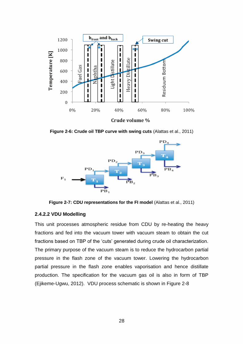
28

Figure 2-6: Crude oil TBP curve with swing cuts (Alattas et al., 2011)

Figure 2-7: CDU representations for the FI model (Alattas et al., 2011)

2.4.2.2 VDU Modelling

This unit processes atmospheric residue from CDU by re-heating the heavy

fractions and fed into the vacuum tower with vacuum steam to obtain the cut

fractions based on TBP of the ‘cuts’ generated during crude oil characterization.

The primary purpose of the vacuum steam is to reduce the hydrocarbon partial

pressure in the flash zone of the vacuum tower. Lowering the hydrocarbon

partial pressure in the flash zone enables vaporisation and hence distillate

production. The specification for the vacuum gas oil is also in form of TBP

(Ejikeme-Ugwu, 2012). VDU process schematic is shown in Figure 2-8

29

Figure 2-8: Process schematic of a typical refinery VDU (Ronald and Colwell, 2010)

Unlike CDU, VDU modelling does not record a large number of publications in

process modelling research (Rodolfo et al., 2010). However, a number of

researchers have used commercial software packages such as Aspen PLUS,

Aspen HYSYS, Aspen PIMS; to generate yields for cut fractions. Ejikeme-Ugwu

(2012) used Aspen HYSYS to obtain yields for vacuum overhead (VO), light

vacuum gas oil (LVGO), heavy vacuum gas oil (HVGO) and vacuum residue

(VR) for different volumetric ratio of crude mixture using rigorous simulation.

2.4.2.3 NHU Modelling

NHU is designed to reduce sulphur content and other impurities in gas oils from

CDU and VDU to the specification of downstream processing units through

hydrodesulphurization (HDS) process (see Figure 2-9 for process schematic).

Product yield from NHU is placed within 95-98 % (Gary andHandwerk, 1984);

this was reported by Ejikeme-Ugwu (2012) based on the fact that not much has

been done in this area of study. However, some researchers worked towards

developing a kinetic model that should be able to estimate the most accurate

operating conditions necessary to achieve sulphur level that meets the desired

specification.

30

Figure 2-9: Process schematic of a typical refinery NHU (Ronald and Colwell,

2010)

López-García and Roy-Auberger (2003) have developed a kinetic model and

conducted experiments adapted to ultra-low sulphur diesel (ULSD) production

for industrial feedstocks. The model is based on a lumped reaction scheme

distinguishing three refractory sulphur families based on Langmuir-Hinshelwood

kinetics. The Langmuir-Hinshelwood representation takes into account the

inhibiting effect of aromatics and nitrogen species on HDS. Their results

indicate a good agreement between most experimental and predicted sulphur

content.

Boesen (2010) investigates diesel hydrotreating reactions and developed a

kinetic model. He used the model to study the kinetics of hydrogenation of

naphthalene on a commercial CoMo catalyst. He further conducted an

experiment at industrial temperatures and pressure, using naphthalene as a

model compound, and found out that intra-particle diffusion resistance might

have impact on the reaction rate.

Jarullah et al. (2011) used optimization techniques to obtain the best values of

kinetic parameters in trickle-bed reactor (TBR) for HDS process based on pilot

31

plant experiment. The technique adopted in their work minimized the sum of the

square errors (SSE) between the experimental and predicted concentrations of

sulphur compound in the products using linear and non-linear regressions

methods. The authors went further to carry out an economic analysis of an

industrial refining unit involving hydrotreatment (Jarullah et al., 2012).

2.4.2.4 FCC Modelling

FCC is employed to produce gasoline from crude oil. FCC typically consist of a

riser where hydrocarbon materials react in the presence of a catalyst, a reactor

to separate gasoline and catalyst, and a regenerator to burn off coke and other

impurities from the used catalyst (Whitcombe et al., 2003; Whitcombe et al.,

2006). The reactivated catalyst are sent back through the riser in a cyclic

process (Kunii and Levenspiel, 1991). Figure 2-10 presents the FCC process

schematic equipped with other facilities (Ronald and Colwell, 2010).

Figure 2-10: Process schematic of a typical refinery FCC (Ronald and Colwell,

2010)

To model FCC, (Gary and Handwerk, 1984) used hand-calculation procedure to

obtain yield correlations to be used in the main planning/scheduling model. The

procedure was reported in Li et al. (2005). Al-Enezi et al. (1999) developed

regression models for predicting product yields and fluid properties for the FCC.

Researchers like Al-Enezi and Elkamel (2000); Michalopoulos et al. (2001) and

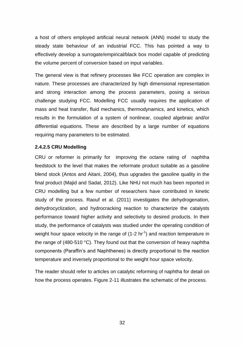
32

a host of others employed artificial neural network (ANN) model to study the

steady state behaviour of an industrial FCC. This has pointed a way to

effectively develop a surrogate/empirical/black box model capable of predicting

the volume percent of conversion based on input variables.

The general view is that refinery processes like FCC operation are complex in

nature. These processes are characterized by high dimensional representation

and strong interaction among the process parameters, posing a serious

challenge studying FCC. Modelling FCC usually requires the application of

mass and heat transfer, fluid mechanics, thermodynamics, and kinetics, which

results in the formulation of a system of nonlinear, coupled algebraic and/or

differential equations. These are described by a large number of equations

requiring many parameters to be estimated.

2.4.2.5 CRU Modelling

CRU or reformer is primarily for improving the octane rating of naphtha

feedstock to the level that makes the reformate product suitable as a gasoline

blend stock (Antos and Aitani, 2004), thus upgrades the gasoline quality in the

final product (Majid and Sadat, 2012). Like NHU not much has been reported in

CRU modelling but a few number of researchers have contributed in kinetic

study of the process. Raouf et al. (2011) investigates the dehydrogenation,

dehydrocyclization, and hydrocracking reaction to characterize the catalysts

performance toward higher activity and selectivity to desired products. In their

study, the performance of catalysts was studied under the operating condition of

weight hour space velocity in the range of (1-2 hr-1) and reaction temperature in

the range of (480-510 °C). They found out that the conversion of heavy naphtha

components (Paraffin’s and Naphthenes) is directly proportional to the reaction

temperature and inversely proportional to the weight hour space velocity.

The reader should refer to articles on catalytic reforming of naphtha for detail on

how the process operates. Figure 2-11 illustrates the schematic of the process.

33

Figure 2-11: Process schematic of a typical refinery CRU (Ronald and Colwell,

2010)

2.4.3 Production with Product Blending

The production with product blending subsystems included gasoline and diesel

blending units in addition to the other main refinery production units (CDU,

VDU, NHU and FCC). The purpose of blending operation is to produce final

products that satisfy quality requirements and demand of a customer and also

meet the environmental regulations set by the government. The goal of

integrating production with product blending is to allow more realistic exchange

of information and flow of material between these subsystems. This generates

more reliable schedules and offers comprehensive cost minimization options

that allow production to follow correct operational sequence. Revenue along

with production schedule, production profile, and inventory levels for component

and product tanks are determined.

Despite the benefit inherent in simultaneous optimization of production with

blending, it appears fewer publications have been reported in this area of

research. Planning/scheduling models for production and products blending

34

subsystems have been developed by Aronofsky et al. (1978); Kendrick et al.

(1981); Moro et al. (1998); Pinto et al. (2000); Joly et al. (2002); Li et al. (2005);

Alattas et al. (2012) and Tong et al. (2012). These methodologies depict the

whole plant topology but the models differ in the way the optimization problem

was formulated, size of the problem, complexity of the units involved and

objectives aim to achieve. Some scheduling models of production with blending

subsystems focused on specific product orders and developed based on a

specific time formulation.

Scheduling model presented by Jia and Ierapetritou (2004) for refinery

production subsystem considers fractionation and reaction processes using

continuous time formulation. The major drawback of their approach is the non-

inclusion of other vital units like FCC, NHU and CRU; making the model

unreliable and hence inaccurate. A simultaneous slot based short-term

scheduling and off-line blending of gasoline products has been reported in

Méndez et al. (2006) in both discrete and continuous time domain in which an

integrated MINLP problem is solved as iterative MILPs. Another MINLP slot

based formulation that relies on iterative MILP solution procedure is the work of

Li et al. (2010). Also, their model is based on gasoline product but incorporate

many real life features like changeovers, non-identical blenders, minimum run

length etc.

Cuiwen et al. (2013) developed mathematical formulations as MINLP and

devises a solution algorithm that solves real world refinery scheduling problems

for production with diesel blending. It is important to note that in real life refinery

operation, other products like gasolines are also blended in addition to the

diesel product grades. Hence, the major setback in their approach is that the

model was developed based on refinery configuration that processes only

diesel products. However, the MINLP model was able to capture both certain

and uncertain events. The model uncertainties are solved using online data

driven rolling horizon strategy.

35

2.5 Refinery Scheduling with Consideration to Uncertainty

Most of the work reported in refinery planning/scheduling are based on

deterministic formulation with less consideration to uncertainties in the model

parameters (Lin et al., 2004). Deterministic models assume that parameters are

known with certainty (Liu and Sahinidis, 1996). Moreover, it has been observed

by Petkov and Maranas (1997) that failure to account for uncertainty in raw

material and product prices, demand and other market conditions could affect

customer satisfaction, high inventory cost and may likely aid business

misfortune. Uncertainty consideration in manufacturing systems could offer a

huge success (Mula et al., 2006).

Different approaches have been proposed in literature to deal with refinery

optimization under uncertainty. For example, stochastic optimization which

could be two-stage or multistage with recourse (Al-Qahtani and Elkamel, 2010;

Liu and Sahinidis, 1996; Sahinidis, 2004) can be employed to deal with

problems in which some uncertain parameters are included in the cost function

and constraints. In stochastic programming, these uncertain parameters are

usually described by probability distributions or by possible scenarios (Clay and

Grossmann, 1997; Liu and Sahinidis, 1996; Ierapetritou and Pistikopoulos,

1996).

The refinery scheduling problems under uncertainty are among the most

challenging optimization problems. Despite their complexity, a number of

research studies have been reported in the literature. A two-stage model to deal

with uncertainties in ship arrival times and demand was proposed by Wang and

Rong (2010). Their work integrates chance-constrained programming and fuzzy

programming in the first stage to develop a model that can be transformed into

a deterministic counterpart and employ a scenario-based framework in the

second stage.

Lin et al. (2004) proposed a novel robust optimization framework to deal with

bounded uncertainty, producing optimal solutions that are immune to changes

in the coefficients of the objective function and changes in the left-hand-side

and right-hand-side parameters of inequality constraints. They extended this

36

idea to address uncertainty with known probability distribution (Janak et al.,

2007). The optimization framework was further extended to a deterministic

robust counterpart model to deal with demand uncertainty (Li et al., 2012b) and

solved using branch and bound global optimization algorithm proposed in (Li et

al., 2012a). Cao et al. (2009) presented chance-constrained stochastic MINLP

and fuzzy programming models for crude oil scheduling under demand

uncertainty.

2.6 Current and Future Directions

Traditionally, uncertainties are considered at the design stage as preventive

measures to ensure schedules generated are reliable under uncertain

operational conditions. Also, reactive measures have to be in place to keep

track of changes in process conditions, constraints, or performance criteria.

Until recently, less attention was given to the scheduling of refinery systems

using control theory. From control point of view, uncertainty can be

accommodated as a disturbance introduced into a system operating at steady

state. Therefore refinery scheduling problems can be formulated and solved in a

closed loop control fashion.

2.6.1 Control Optimization Strategies as Viable Alternatives

Various alternative formulations have been proposed in modelling supply chain

problems under uncertainty. Control theories provide sufficient mathematical

tools to address uncertainty in process systems (Sarimveis et al., 2008). In

scheduling problems, system dynamics are defined using discrete time

representations, material balance, and component balance while updating state

of the system based on current value of the uncertain parameter. In reality,

solution procedure under particular framework mimics close loop feedback

control structure as actions to be taken at any time instant depend on the output

value at previous times. Uncertainty (disturbance) affects the system states like

flowrates, inventory levels, and schedule generated considering the entire

uncertain parameter space is adjudged to be robust.

37

From process point of view, two types of uncertainties are to be expected:

endogenous uncertainties that manifest when operators have little knowledge

about the process itself, for example kinetic parameters of reaction system,

mass transfer rate in CDU, etc. and exogenous uncertainties introduced

externally but have impacts on the process. In refinery systems, exogenous

uncertainties could be crude oil feed rate, composition, fuel products recycled

into the system, composition of additives used in blending units etc. In this work,

uncertainties due to crude oil feed rate and crude oil composition were

addressed.

2.6.1.1 Receding horizon

Receding horizon under the framework of model predictive control has been

reported for production scheduling as a powerful tool to address disruptive

events. Kopanos and Pistikopoulos (2014) developed a solution procedure that

works with multiparametric programming to address uncertainty for systems

with bounded uncertain parameters. Their approach suffers a major setback as

problems involving MINLP was out of their consideration. However, the concept

proposed is still promising in that large scale optimization problems can be

solved.

Receding horizon has been applied successfully in Goodwin et al. (2006) to

address mining problems. Non-uniform time discretization was proposed to

formulate the problem described using state-space representation. The dynamic

model captures real time issues and uses mining action as control input. In

Munawar and Gudi (2005), receding horizon was considered as a tool for

handling disruptive effects on reactive scheduling. Problems were formulated at

different levels to verify the robustness of the control theory approach in

generating reliable schedules.

In Yüzgeç et al. (2010), a model predictive control strategy was presented to

address uncertainty in demand of crude oil from blending tanks using moving

horizon control strategy. The solution procedure adopted in the paper is similar

to moving end control strategy employed in this work to compare with our fixed

end horizon approach. Their approach is not a good option for customers with

38

fixed deadline due to low degree of freedom as solution search does not cover

the entire length of the scheduling horizon. In production area of refinery,

Cuiwen et al. (2013) used similar approach successfully.

More detail about this methodology will be given in Chapter 4.

2.6.1.2 Self-optimizing control

Self-optimizing control strategy (SOC) has been a technique to deal with

uncertainty in most chemical processes. Although it records a significant

number of publications, the concept has never been applied in petroleum

refinery scheduling. It has been shown in Kariwala (2007); Alstad and

Skogestad (2007); Kariwala et al. (2008); Jäschke and Skogestad (2011); Ye et

al. (2012a); and Ye et al. (2012b) that SOC is a reliable technique for solving

problems with uncertainty in process parameters. Applying the solution strategy

on refinery production problems should result in generating optimal schedules

globally.

Using SOC, controlled variables (CV) can be selected so that when they are

maintained at constant set points the overall plant operation is optimal or near

optimal despite various uncertainties. In this study, the focus will be on

maintaining the gradient of the cost function at zero via Taylor series

approximation of CVs over the whole parameter space. The CV should

approximate the gradient adequately (Ye et al., 2012b). The detail of the

methodology and how it works will be discussed in Chapter 6.

2.6.2 An Integrated Approach

Several models for planning and scheduling of refinery systems are reported

separately in literature. The two decision levels are interwoven with scheduling

mainly executing orders set by planning. A model that integrates planning and

scheduling will improve the efficiency and profitability of a refinery business. An

integrated planning and scheduling with consideration to endogenous and

exogenous uncertainties will aid more reliable decisions. This motivates some

researchers to exploit different ways to model and solve the plant-wide

problems. Few research studies reported include Mouret et al. (2011);

39

Verderame et al. (2010); Munawar and Gudi (2005); Pinto et al. (2000); Joly et

al. (2002); and Luo and Rong (2009).

In most of the work reviewed in refinery planning and scheduling, exogenous

uncertainties predominate. However, there is also a need to consider

endogenous uncertainties as they affect the quality and economics of the

overall production.

2.7 Summary of Knowledge Gap in Refinery Scheduling

Below are the highlights of the knowledge gap this research study finds worthy

to fill.

Models developed previously have shortcomings in one way or the other

that practical implementation of decisions obtained from solving the

models may fail to reflect realities. Therefore there is the need to develop

a more reliable model for crude oil scheduling.

While mathematical techniques for refinery planning have a long

established presence in petroleum research studies, much less has been

reported in scheduling of production area. Accurate model for

simultaneous optimization of production with product blending is

necessary in order to generate optimal schedules at minimum cost.

Generally, crude oil refinery operates under economic and environmental

conditions bounded with uncertainties. Models which take into

cognizance a number of uncertainties can be expected to generate

reliable decisions. In most of the work reported in refinery scheduling,

uncertainties from design point of view predominate. However, there is

also a need to consider operational uncertainties (uncertainty in the form

of disturbance) as they affect the accuracy and robustness of the overall

schedule.

This study fills these gaps as discussed in Section 1.4 of the introductory

chapter. Work done to address the issues raised will be reported in

Chapters 3, 4, 5 and 6.

41

3 MODELLING CRUDE OIL UNLOADING AREA

Being an integral part of the refinery supply chain, optimization of crude oil

refining processes promises a big cut in operational and logistic costs of the

whole refinery plant. Better economic performance is achieved by developing

robust procedures for short-term scheduling of material flow in crude oil

unloading area. The work in this chapter is on the modelling, investigating the

model performance through case studies, and schedule generation under

uncertain conditions.

In research studies, crude oil scheduling problems are often formulated as

optimization model with operating cost as the objective function. The challenge

with building models for crude oil scheduling lies in knowing and including what

is relevant for the specific decisions that are to be made using the model and

neglecting the elements that are not relevant. Selection of units with

arrangements on the sequence of operation with regards to modelling of crude

oil scheduling problems requires a systematic approach.

Since scheduling of crude oil operations usually involves discrete and

continuous decisions (e.g. vessel unloading, tank switching, flow of mixed

crude, etc.), mixed integer linear programming (MILP) or mixed integer

nonlinear programming (MINLP) are used in formulating the optimization

problem. A significant number of techniques were developed for generating

schedules in this area of study. However, there is still a gap of knowledge that

needs to be bridged towards the development of more reliable procedures that

are not only acceptable to the planning team but also have the capability for

guaranteeing performance during execution in the real refinery plant. Model

presented in Lee et al. (1996) has been a benchmark upon which other crude

oil scheduling models were built. This research study also finds the model

suitable for used in generating schedules under uncertainty.

In this chapter, a methodology for short-term crude oil unloading, tank inventory

management, and crude distillation unit (CDU) charging is developed as an

extension to Lee et al. (1996) model. The extended model considers real life

42

issues not captured in the original model and was developed through

reformulation in which the problem statement was modified to account for

certain details. The performance of the extended model was assessed through

case studies. The reformulation was based on established operating rules in

petroleum refineries, material balances, resource allocations, sequencing order,

product quality, and demand of mixed crude oil.

Scenarios were created to offer recommendations to plant operators on the best

schedule to use. Uncertainties due to disruptive events (CDU shutdown), and

low inventory at the scheduling horizon were also considered.

3.1 Model Formulation for Crude Oil Scheduling

3.1.1 Problem Definition

Same as in Lee et al. (1996), this study considers a coastal refinery with

docking stations (where the crude vessels unload their content), storage tanks

(for holding crude oil before transfer to charging tanks), and charging tanks

where blending operation is carried out for subsequent transfer to CDUs in

accordance with the CDUs mixed crude oil quality requirements. These transfer

operations are achieved in different units/facilities interconnected by means of a

pipe network. Throughout the scheduling horizon, industry operational practice

is observed. The following technical details are available to adequately define

the crude oil scheduling problem.

Number of vessels, amount and crude oil parcel conveyed and the arrival

and departure times of each vessel.

Number of units/facilities for the crude oil transfer from vessel down to

the CDU with their capacity limits, initial inventory levels and

interconnections.

Upper and lower bounds on the stream flows across the connecting

units/facilities.

Specification of key components with their permissible concentration

ranges.

43

Information on dedication of certain tanks for receiving specific crude oil

types.

Other information such as CDUs demand of mixed crude oil from

charging tanks, unloading and sea waiting costs of vessels, inventory

costs for charging and storage tanks, tank-tank set up cost, changeover

cost, and shutdown cost for CDUs.

With the information above, the scheduling problem is to minimize the overall

cost of operation by determining the following optimization variables:

Waiting time for each vessel until the unloading process begins.

Unloading duration for each vessel.

Volume per unit time of crude oil unloaded for each vessel.

Volumes per unit time of crude oil transferred from vessels to storage

tanks then to charging tanks and finally to CDUs.

Vessels, storage and charging tanks’ inventory levels at each time

interval within the scheduling horizon.

CDU charging rates.

Time and sequence of charging mixed crude oil into each CDU.

Time and sequence of crude oil transfer from storage tanks to charging

tanks.

Concentration of key component (such as sulphur) in charging tanks.

3.1.2 Model Assumptions

Same as in Lee et al. (1996), Li et al. (2007), Yüzgeç et al. (2010), Reddy et al.

(2003), and Pan et al. (2009); the following assumptions are considered in this

section.

1. The unloading operation is carried out in only one docking station.

2. Volume of crude oil remaining in the pipeline is negligible compared to

the total volume processed in the entire scheduling horizon.

3. The time for change-over is negligible compared to the entire scheduling

horizon.

4. Perfect mixing occurs in the charging tank and mixing time is negligible.

44

5. Continuous demand order matches the limits of the CDU operations.

3.1.3 Objective Function

The objective function is the cost function to be minimized, which includes

unloading and sea waiting costs for the crude oil vessels, the storage and

charging tanks’ inventory costs, changeover cost and the penalties for CDU

shutdown and tank-tank transfer.

𝐶𝑂𝑃𝑅 = 𝐶𝑈𝑁𝐿𝑣 ∑(𝑇𝐿𝑣 − 𝑇𝐹𝑣)

𝑁𝑉

𝑣=1

+ 𝐶𝑆𝐸𝐴𝑣 ∑(𝑇𝐹𝑣 − 𝑇𝐴𝑅𝑅,𝑣)

𝑁𝑉

𝑣=1

+ 𝐶𝐼𝑁𝑆𝑇𝑖 ∑ ∑ (𝑉𝑆𝑖,𝑡 + 𝑉𝑆𝑖,𝑡−1

2)

𝑁𝑆𝐶𝐻

𝑡=1

𝑁𝑆𝑇

𝑖=1

+ 𝐶𝐼𝑁𝐵𝑇𝑗 ∑ ∑ (𝑉𝐵𝑗,𝑡 + 𝑉𝐵𝑗,𝑡−1

2)

𝑁𝑆𝐶𝐻

𝑡=1

𝑁𝐵𝑇

𝑗=1

+ ∑ ∑ ∑ (𝐶𝐶 × 𝑍𝑗,𝑙,𝑡)

𝑁𝑆𝐶𝐻

𝑡=1

𝑁𝐶𝐷𝑈

𝑙=1

𝑁𝐵𝑇

𝑗=1

+ ∑ ∑ 𝐶𝐷 × 𝑋𝐷𝑙,𝑡

𝑁𝑆𝐶𝐻

𝑡=1

𝑁𝐶𝐷𝑈

𝑙=1

+ ∑ ∑ 𝐶𝑆 × 𝑋𝑆𝑖,𝑡

𝑁𝑆𝐶𝐻

𝑡=1

𝑁𝑆𝑇

𝑖=1

(3-1)

In Equation 3-1, the unloading cost of crude vessels (𝑣 = 1 to 𝑁𝑉) is the

product of unloading cost per unit time interval, 𝐶𝑈𝑁𝐿𝑣 and unloading duration

(vessel departure time 𝑇𝐿𝑣 minus vessel unloading initiation time 𝑇𝐹𝑣). Similarly,

the sea waiting cost of crude vessels (𝑣 = 1 to 𝑁𝑉) is the product of sea

waiting cost per unit time interval, 𝐶𝑆𝐸𝐴𝑣 and waiting duration (vessel unloading

initiation time 𝑇𝐹𝑣 minus vessel arrival time 𝑇𝐴𝑅𝑅,𝑣).

The storage tanks inventory cost is computed by multiplying the cost per unit

time per unit volume, 𝐶𝐼𝑁𝑆𝑇𝑖 of tanks (𝑖 = 1 to 𝑁𝑆𝑇) over the interval length

(𝑡 = 1 to 𝑁𝑆𝐶𝐻) with the average tanks’ volumes 𝑉𝑆𝑖,𝑡 at two successive time

periods 𝑡 and 𝑡 − 1. Charging tanks (𝑗 = 1 to 𝑁𝐵𝑇) inventory cost is computed

45

in a similar way with 𝑉𝐵𝑗,𝑡 as the tanks’ volume at time period 𝑡. 𝐶𝐼𝑁𝐵𝑇𝑗 is the

cost per unit time per unit volume.

The changeover cost for CDUs (𝑙 = 1 to 𝑁𝐶𝐷𝑈) is proportional to the number

of blended crude oil switching given by the binary variable 𝑍𝑗,𝑙,𝑡 with 𝐶𝐶 as the

cost for each switch operation. When there is CDU shutdown as discussed in

one of the scenarios in this chapter, a binary variable 𝑋𝐷𝑙,𝑡 is activated and is

penalized with 𝐶𝐷 as the cost. A binary variable 𝑋𝑆𝑖,𝑡 is activated whenever

there is a tank-tank transfer operation. 𝐶𝑆 represents the cost penalty for each

transfer operation.

3.1.4 Constraints

3.1.4.1 Rules of operation

Vessel unloading sequence

The arrival and departure of crude oil vessel at the docking station, takes place

only once throughout the scheduling horizon.

∑ 𝑋𝐹𝑣,𝑡

𝑁𝑆𝐶𝐻

𝑡=1

= 1 𝑣 = 1,… ,𝑁𝑉

(3-2)

∑ 𝑋𝐿𝑣,𝑡

𝑁𝑆𝐶𝐻

𝑡=1

= 1 𝑣 = 1,… ,𝑁𝑉 (3-3)

The unloading process of each crude oil vessel must be after it arrives at the

docking station as determined at the planning level.

𝑇𝐹𝑣 ≥ 𝑇𝐴𝑅𝑅,𝑣 𝑣 = 1,… ,𝑁𝑉 (3-4)

The following two equations defined vessel initiation and completion times.

𝑇𝐹𝑣 = ∑ 𝑡𝑋𝐹𝑣,𝑡

𝑁𝑆𝐶𝐻

𝑡=1

𝑣 = 1,… ,𝑁𝑉 (3-5)

46

𝑇𝐿𝑣 = ∑ 𝑡𝑋𝐿𝑣,𝑡

𝑁𝑆𝐶𝐻

𝑡=1

𝑣 = 1,… ,𝑁𝑉 (3-6)

Based on the assumption that there is only one docking station, two vessels

cannot unload crude oil at the same time. Therefore a vessel must finish

unloading one time interval before the next vessel begins to unload.

𝑇𝐹𝑣+1 ≥ 𝑇𝐿𝑣 + 1 𝑣 = 1,… ,𝑁𝑉 (3-7)

A vessel unloading is accomplished between the time intervals 𝑇𝐹𝑣 and 𝑇𝐿𝑣 .

𝑋𝑊𝑣,𝑖,𝑡 ≤ ∑ 𝑋𝐹𝑣,𝑚

𝑡

𝑚=1

, 𝑋𝑊𝑣,𝑖,𝑡 ≤ ∑ 𝑋𝐿𝑣,𝑚

𝑁𝑆𝐶𝐻

𝑚=𝑡

𝑣 = 1,… ,𝑁𝑉, 𝑡 = 1,… ,𝑁𝑆𝐶𝐻

(3-8)

The binary variable 𝑋𝑊𝑣,𝑖,𝑡 takes on value of 1 when crude oil vessel 𝑣 is

unloading to storage tank at time 𝑡.

The unloading duration is bounded by the two time intervals 𝑇𝐹𝑣 and 𝑇𝐿𝑣.

𝑇𝐿𝑣 − 𝑇𝐹𝑣 ≥ 1 𝑣 = 1,… ,𝑁𝑉 (3-9)

Standing gauge operation: this forbids flow in and out of tanks

simultaneously. When the binary variable 𝑋𝑊𝑆𝑖,𝑗,𝑡 is equal to 1, it means

storage tank 𝑖 is feeding charging tank 𝑗 at time t and therefore that storage tank

𝑖 cannot receive crude oil from vessel 𝑣 at that period of time 𝑡. In such a

situation the binary variable 𝑋𝑊𝑣,𝑖,𝑡 for crude transfer to storage tank 𝑖 must be

0.

𝑋𝑊𝑆𝑖,𝑗,𝑡 ≤ 1 − 𝑋𝑊𝑣,𝑖,𝑡

𝑣 = 1, … , 𝑁𝑉, 𝑖 = 1, … ,𝑁𝑆𝑇, 𝑗 = 1,… ,𝑁𝐵𝑇, 𝑡 = 1, … , 𝑁𝑆𝐶𝐻

(3-10)

Similarly, charging tanks cannot feed CDU when its receiving crude oil from

storage tank forcing the variable 𝐷𝑗,𝑙,𝑡 for CDU charging to be 0.

𝐷𝑗,𝑙,𝑡 ≤ 1 − 𝑋𝑊𝑆𝑖,𝑗,𝑡 (3-11)

47

𝑖 = 1, … ,𝑁𝑆𝑇, 𝑗 = 1,… ,𝑁𝐵𝑇, 𝑙 = 1,… ,𝑁𝐶𝐷𝑈, 𝑡 = 1, … , 𝑁𝑆𝐶𝐻

Semi-continuous constraints: these are applied for feedstock to CDU 𝐹𝐵𝐶𝑗,𝑙,𝑡

to ensure that operation of the CDU is within the design flow rate and assumes

no flow when CDU shuts down.

For normal operation the constraint is:

𝐹𝐵𝐶𝑚𝑖𝑛𝑗,𝑙 ≤ 𝐹𝐵𝐶𝑗,𝑙,𝑡 ≤ 𝐹𝐵𝐶𝑚𝑎𝑥𝑗,𝑙

𝑗 = 1, … , 𝑁𝐵𝑇, 𝑙 = 1,… ,𝑁𝐶𝐷𝑈, 𝑡 = 1, … , 𝑁𝑆𝐶𝐻

(3-12)

When CDU shuts down,

𝐹𝐵𝐶𝑗,𝑙,𝑡 = 0

𝑗 = 1,… ,𝑁𝐵𝑇, 𝑙 = 1,… ,𝑁𝐶𝐷𝑈, 𝑡 = 1, … , 𝑁𝑆𝐶𝐻

(3-13)

Flow constraint from storage tank to charging tank: for multiple storage

tanks feeding charging tank (s), a pipeline can only be lined up to just one

charging tank at a time. The total quantity received by charging tank (s) must

not exceed the maximum flow rate from storage tanks. For connecting pipeline

between storage and charging tanks when storage tanks are feeding charging

tanks at the rate 𝐹𝑆𝐵𝑖,𝑗,𝑡 the constraint is represented as:

∑ 𝐹𝑆𝐵𝑖,𝑗,𝑡 ≤

𝑁𝑆𝑇

𝑖

𝐹𝑆𝐵𝑚𝑎𝑥𝑖,𝑗

𝑖 = 1, … , 𝑁𝑆𝑇, 𝑗 = 1,… ,𝑁𝐵𝑇, 𝑡 = 1, … , 𝑁𝑆𝐶𝐻

(3-14)

Demand violation constraints: unlike in Lee et al. (1996) a violation in

demand order is introduced here to make the model more flexible. This is

necessary because the model becomes infeasible where supply failed to meet

the exact demand. For demand of crude oil mix 𝑞 from charging tank 𝑗,

Equation 3-15 represents supply to meet exact or below actual demand and

Equation 3-16 to account for supply to meet the exact or above actual demand.

48

∑ ∑ 𝐹𝐵𝐶𝑗,𝑙,𝑡 ≥ 𝐷𝑀𝑞(1 − 𝜀1𝑞)

𝑁𝑆𝐶𝐻

𝑡=1

𝑁𝐶𝐷𝑈

𝑙=1

𝑗 = 1,… ,𝑁𝐵𝑇, 𝑞 = 1,… ,𝑁𝐵𝑇

(3-15)

and,

∑ ∑ 𝐹𝐵𝐶𝑗,𝑙,𝑡 ≤ 𝐷𝑀𝑞(1 + 𝜀2𝑞)

𝑁𝑆𝐶𝐻

𝑡=1

𝑁𝐶𝐷𝑈

𝑙=1

𝑗 = 1,… ,𝑁𝐵𝑇, 𝑞 = 1,… ,𝑁𝐵𝑇

(3-16)

𝜀1𝑞 is a parameter that specifies the demand violation of crude mix q in the

negative direction (below the actual demand) and 𝜀2𝑞 specifies the demand

violation of crude mix 𝑞 in the positive direction (above the actual demand).

When each of these parameters is 0, a demand violation is not allowed and

when it is 1, a 100% violation in demand order is allowed. With these

parameters, it is possible to carry out a sensitivity analysis to determine the

maximum value of demand violation of each crude mix that will maintain the

optimal solution of the MILP scheduling model.

Continuous flow constraint: at any time, one charging tank should be

charging the CDU.

∑ 𝐷𝑗,𝑙,𝑡 = 1

𝑁𝐵𝑇

𝑗

𝑙 = 1,… ,𝑁𝐶𝐷𝑈, 𝑡 = 1,… ,𝑁𝑆𝐶𝐻

(3-17)

Flow fluctuation constraints: widely varying interval-interval CDUs charging

rate should be avoided because it disrupts CDU operation and may generate off

specification cuts. Two constraints are imposed to limit the interval-interval

variation in quantity fed to the CDU. These are:

49

𝐹𝐵𝐶𝑗,𝑙,𝑡−1 ≥ 𝐹𝐵𝐶𝑗,𝑙,𝑡(1 − 𝛽𝑙)

𝑗 = 1,… ,𝑁𝐵𝑇, 𝑙 = 1,… ,𝑁𝐶𝐷𝑈, 𝑡 = 1,… ,𝑁𝑆𝐶𝐻 − 1

(3-18)

and

𝐹𝐵𝐶𝑗,𝑙,𝑡−1 ≤ 𝐹𝐵𝐶𝑗,𝑙,𝑡(1 + 𝛽𝑙)

𝑗 = 1,… ,𝑁𝐵𝑇, 𝑙 = 1,… ,𝑁𝐶𝐷𝑈, 𝑡 = 1,… ,𝑁𝑆𝐶𝐻 − 1

(3-19)

𝛽𝑙 is a user defined parameter with values ranging between zero and one. If 𝛽𝑙

is set at zero, no variation in interval-interval quantity while setting it to 1 implies

that 100% variation is permitted. For the cases in this thesis a conservative

value of 0.1 is used.

Changeover penalty: this is to consider a cost associated with switching of

charging tanks any time it occurs. Lee et al. (1996) represents changeover as a

point when a charging tank 𝑗 at time 𝑡 − 1 charges the CDU followed by another

charging tank 𝑔 at a later time 𝑡.

𝑍𝑗,𝑔,𝑙,𝑡 ≥ 𝐷𝑔,𝑙,𝑡 + 𝐷𝑗,𝑙,𝑡−1 − 1

𝑗, 𝑔(𝑗 ≠ 𝑔) = 1,… ,𝑁𝐵𝑇, 𝑙 = 1,… ,𝑁𝐶𝐷𝑈, 𝑡 = 1,… ,𝑁𝑆𝐶𝐻 − 1

(3-20)

Equation 3-20 results in a large number of integer variables and constraints,

making it computationally expensive for problems involving multiple CDUs. An

improvement over this by Li et al. (2002) overcomes the challenge by reducing

the changeover penalty variable 𝑍𝑗,𝑔,𝑙,𝑡 from a tetra-indexed variable to a tri-

index variable 𝑍𝑗,𝑙,𝑡. A simple approach adopted in their paper suggests the use

of Equations 3-21 and 3-22.

𝑍𝑗,𝑙,𝑡 ≥ 𝐷𝑗,𝑙,𝑡 − 𝐷𝑗,𝑙,𝑡−1

𝑗 = 1,… ,𝑁𝐵𝑇, 𝑙 = 1,… ,𝑁𝐶𝐷𝑈, 𝑡 = 1,… ,𝑁𝑆𝐶𝐻 − 1

(3-21)

𝑍𝑗,𝑙,𝑡 ≥ 𝐷𝑗,𝑙,𝑡−1 − 𝐷𝑗,𝑙,𝑡 (3-22)

50

𝑗 = 1,… ,𝑁𝐵𝑇, 𝑙 = 1,… ,𝑁𝐶𝐷𝑈, 𝑡 = 1,… ,𝑁𝑆𝐶𝐻 − 1

The term 𝐶𝐶 × 𝑍𝑗,𝑙,𝑡 is added to the objective function. 𝐶𝐶 is the cost penalty for

changeover.

Shutdown constraints: these are included to permit generating flexible

schedules involving both shutdown and continual operations. Thus,

𝐹𝐵𝐶𝑗,𝑙,𝑡 ≥ (1 − 𝑋𝐷𝑙,𝑡)𝐹𝐵𝐶𝑙𝑜𝑗,𝑙,𝑡

𝑗 = 1,… ,𝑁𝐵𝑇, 𝑙 = 1,… ,𝑁𝐶𝐷𝑈, 𝑡 = 1,… ,𝑁𝑆𝐶𝐻 − 1

(3-23)

𝐹𝐵𝐶𝑗,𝑙,𝑡 ≤ (1 − 𝑋𝐷𝑙,𝑡)𝐹𝐵𝐶𝑢𝑝𝑗,𝑙,𝑡

𝑗 = 1,… ,𝑁𝐵𝑇, 𝑙 = 1,… ,𝑁𝐶𝐷𝑈, 𝑡 = 1,… ,𝑁𝑆𝐶𝐻 − 1

(3-24)

The binary variable 𝑋𝐷𝑙,𝑡 is zero during normal operation and takes on the value

of 1 when CDU shuts down. The minimum flow rate threshold before CDU

deemed to have shutdown, 𝐹𝐵𝐶𝑙𝑜𝑗,𝑙,𝑡 is the lower bound on the flow FBC with

𝐹𝐵𝐶𝑢𝑝𝑗,𝑙,𝑡 being the upper bound. The term 𝐶𝐷 × 𝑋𝐷𝑙,𝑡 is added to the objective

function. 𝐶𝐷 is the cost penalty for shutdown. With this constraint and penalty, a

schedule can also be generated with one or more CDU not in operation. The

implication is that uncertainty due to disruption in CDU operation has been

taken care of and therefore will have no effect on the execution of the schedule

should the uncertain event occur at any time within the scheduling horizon. The

scenario to support this is considered in Case 3.

Set-up constraint: in real life situation, tank-tank transfer involves some

activities when a crude vessel is allowed to unload into multiple storage tanks

for subsequent transfer of the crude oil into charging tanks. A set-up cost is

incurred anytime switching occurs between storage tanks and charging tanks.

Including a set-up cost for these activities in the objective function minimizes the

number of these activities.

51

𝑋𝑆𝑖,𝑡 ≥ 𝑋𝑊𝑆𝑖,𝑗,𝑡 − 𝑋𝑊𝑆𝑖,𝑗,𝑡−1

𝑖 = 1, … ,𝑁𝑆𝑇, 𝑗 = 1,… ,𝑁𝐵𝑇, 𝑡 = 1, … , 𝑁𝑆𝐶𝐻 − 1

(3-25)

This set-up cost is considered in Case 3 with more storage and charging tanks

translating into a quite number of switchover operations. The term 𝐶𝑆 × 𝑋𝑆𝑖,𝑡 is

added to the objective function for this case. 𝐶𝑆 is the cost penalty for switching

from tank to tank during tank-tank transfers. The binary variable 𝑋𝑆𝑖,𝑡 is

activated whenever there is a tank-tank transfer operation

3.1.4.2 Hydraulic capacities

Flow constraints: flow of crude oil is bounded by the capacity of the pumping

system available. For the main units/facilities for crude oil transfer, the following

holds:

For crude oil flow from vessel to storage tank 𝐹𝑉𝑆𝑣,𝑖,𝑡 the following relation holds

𝐹𝑉𝑆𝑚𝑖𝑛𝑣,𝑖𝑋𝑊𝑣,𝑖,𝑡 ≤ 𝐹𝑉𝑆𝑣,𝑖,𝑡 ≤ 𝐹𝑉𝑆𝑚𝑎𝑥𝑣,𝑖𝑋𝑊𝑣,𝑖,𝑡

𝑣 = 1,… , 𝑁𝑉, 𝑖 = 1, … ,𝑁𝑆𝑇, 𝑡 = 1,… ,𝑁𝑆𝐶𝐻

(3-26)

Similarly, for crude oil transfer from storage tank to charging tank 𝐹𝑆𝐵𝑣,𝑖,𝑡,

𝐹𝑆𝐵𝑚𝑖𝑛𝑖,𝑗𝑋𝑊𝑆𝑖,𝑗,𝑡 ≤ 𝐹𝑆𝐵𝑖,𝑗,𝑡 ≤ 𝐹𝑆𝐵𝑚𝑎𝑥𝑖,𝑗𝑋𝑊𝑆𝑖,𝑗,𝑡

𝑖 = 1, … , 𝑁𝑆𝑇, 𝑗 = 1,… ,𝑁𝐵𝑇, 𝑡 = 1,… ,𝑁𝑆𝐶𝐻

(3-27)

Flow from charging tank to CDU,

𝐹𝐵𝐶𝑚𝑖𝑛𝑗,𝑙𝐷𝑗,𝑙,𝑡 ≤ 𝐹𝐵𝐶𝑗,𝑙,𝑡 ≤ 𝐹𝐵𝐶𝑚𝑎𝑥𝑗,𝑙𝐷𝑗,𝑙,𝑡

𝑗 = 1,… ,𝑁𝐵𝑇, 𝑙 = 1,… ,𝑁𝐶𝐷𝑈, 𝑡 = 1,… ,𝑁𝑆𝐶𝐻

(3-28)

Capacity constraints: the volume of crude oil in storage 𝑉𝑆𝑖,𝑡 and charging

tanks 𝑉𝐵𝑗,𝑡 at any time must be within the upper and lower bounds of the

containing medium.

52

The capacity limitation for storage tank is:

𝑉𝑆𝑚𝑖𝑛𝑖 ≤ 𝑉𝑆𝑖,𝑡 ≤ 𝑉𝑆𝑚𝑎𝑥𝑖

𝑖 = 1, … ,𝑁𝑆𝑇, 𝑡 = 1, … , 𝑁𝑆𝐶𝐻

(3-29)

and for charging tank,

𝑉𝐵𝑚𝑖𝑛𝑗 ≤ 𝑉𝐵𝑗,𝑡 ≤ 𝑉𝐵𝑚𝑎𝑥𝑗

𝑗 = 1,… ,𝑁𝐵𝑇, 𝑡 = 1,… ,𝑁𝑆𝐶𝐻

(3-30)

Crude oil material balance

Crude oil vessel: volume 𝑉𝑉𝑣,𝑡 of crude oil in vessel 𝑣 at time 𝑡 equals the

difference between the initial crude volume and the overall volume transferred

from the vessel up to time 𝑡. 𝑉𝑉𝑣,0 is the volume at time 0.

𝑉𝑉𝑣,𝑡 = 𝑉𝑉𝑣,0 − ∑ ∑ 𝐹𝑉𝑆𝑣,𝑖,𝑚

𝑡

𝑚=1

𝑁𝑆𝑇

𝑖=1

𝑣 = 1,… ,𝑁𝑉, 𝑡 = 1,… ,𝑁𝑆𝐶𝐻

(3-31)

For the whole scheduling horizon, the equation becomes:

𝑉𝑉𝑣,0 = ∑ ∑ 𝐹𝑉𝑆𝑣,𝑖,𝑡

𝑁𝑆𝐶𝐻

𝑡=1

𝑁𝑆𝑇

𝑖=1

𝑣 = 1,… ,𝑁𝑉

(3-32)

At any time period within the scheduling horizon, the following equation holds

for crude oil vessels.

𝐹𝑉𝑆𝑣,𝑖,𝑡 ≤ 𝑉𝑉𝑣,𝑡

𝑣 = 1,… , 𝑁𝑉, 𝑖 = 1, … ,𝑁𝑆𝑇, 𝑡 = 1,… ,𝑁𝑆𝐶𝐻

(3-33)

Storage tank: Volume 𝑉𝑆𝑖,𝑡 of crude oil in storage tank 𝑖 at time 𝑡 equals the

sum of the initial volume stored in the storage tank with the volume transferred

53

into the storage tank up to time 𝑡, less volume transferred from the storage tank

up to time 𝑡. 𝑉𝑆𝑖,0 is the volume at time 0.

𝑉𝑆𝑖,𝑡 = 𝑉𝑆𝑖,0 + ∑ ∑ 𝐹𝑉𝑆𝑣,𝑖,𝑚 − ∑ ∑𝐹𝑆𝐵𝑖,𝑗,𝑚

𝑡

𝑚=1

𝑁𝐵𝑇

𝑗=1

𝑡

𝑚=1

𝑁𝑉

𝑣=1

𝑖 = 1, … ,𝑁𝑆𝑇, 𝑡 = 1, … , 𝑁𝑆𝐶𝐻

(3-34)

At any time period within the scheduling, the following equation holds for

storage tanks.

𝐹𝑆𝐵𝑖,𝑗,𝑡 ≤ 𝑉𝑆𝑖,𝑡

𝑖 = 1, … ,𝑁𝑆𝑇, 𝑗 = 1,… ,𝑁𝐵𝑇, 𝑡 = 1,… ,𝑁𝑆𝐶𝐻

(3-35)

Charging tank: Volume 𝑉𝐵𝑗,𝑡 of crude mix in charging tank 𝑗 at time 𝑡 equals the

sum of the initial volume of crude mix in the charging tank with the volume

transferred into the charging tank up to time 𝑡, less volume transferred from the

charging tank up to time 𝑡. 𝑉𝐵𝑗,0 is the volume at time 0.

𝑉𝐵𝑗,𝑡 = 𝑉𝐵𝑗,0 + ∑ ∑ 𝐹𝑆𝐵𝑖,𝑗,𝑚 − ∑ ∑ 𝐹𝐵𝐶𝑗,𝑙,𝑚

𝑡

𝑚=1

𝑁𝐶𝐷𝑈

𝑙=1

𝑡

𝑚=1

𝑁𝑆𝑇

𝑖=1

𝑗 = 1,… ,𝑁𝐵𝑇, 𝑡 = 1,… ,𝑁𝑆𝐶𝐻

(3-36)

At any time period within the scheduling, the following equation holds for

charging tanks.

𝐹𝐵𝐶𝑗,𝑙,𝑡 ≤ 𝑉𝐵𝑗,𝑡

𝑗 = 1,… ,𝑁𝐵𝑇, 𝑙 = 1,… ,𝑁𝐶𝐷𝑈, 𝑡 = 1,… ,𝑁𝑆𝐶𝐻

(3-37)

Component material balance: the component material balance in storage

tanks should only be used when there is mixing in storage tank due to difficulty

in segregating crudes of different compositions. The mixing here is not the

same as blending operation as the latter is limited to charging tanks only.

Storage tank: volume 𝑣𝑠𝑘,𝑖,𝑡 of component 𝑘 in storage tank 𝑖 at time 𝑡 equals

the sum of volume of component 𝑘 in the storage tank with the volume of

54

component 𝑘 transferred into the storage tank up to time 𝑡, less volume of

component 𝑘 transferred from the storage tank up to time 𝑡. 𝑣𝑠𝑘,𝑖,0 is the volume

at time 0.

𝑣𝑠𝑘,𝑖,𝑡 = 𝑣𝑠𝑘,𝑖,0 + ∑ ∑ 𝑓𝑣𝑠𝑘,𝑣,𝑖,𝑚

𝑁𝑉

𝑣=1

𝑡

𝑚=1

− ∑ ∑ 𝑓𝑠𝑏𝑘,𝑖,𝑗,𝑚

𝑁𝐵𝑇

𝑗=1

𝑡

𝑚=1

𝑘 = 1,… ,𝑁𝐶𝑂𝑀𝑃, 𝑖 = 1, … , 𝑁𝑆𝑇, 𝑡 = 1,… ,𝑁𝑆𝐶𝐻

(3-38)

Component volumetric flow from vessel to storage tank

𝑓𝑣𝑠𝑘,𝑣,𝑖,𝑡 = 𝐹𝑉𝑆𝑣,𝑖,𝑡 𝑤𝑣𝑘,𝑣

𝑘 = 1, … , 𝑁𝐶𝑂𝑀𝑃, 𝑣 = 1, … ,𝑁𝑉, 𝑖 = 1, … ,𝑁𝑆𝑇, 𝑡 = 1,… ,𝑁𝑆𝐶𝐻

(3-39)

Charging tank: volume 𝑣𝑏𝑘,𝑗,𝑡 of component 𝑘 in charging tank 𝑗 at time 𝑡 equals

the sum of volume of component 𝑘 in the charging tank with the volume of

component 𝑘 transferred into the charging tank up to time 𝑡, less volume of

component 𝑘 transferred from the charging tank up to time 𝑡. 𝑣𝑏𝑘,𝑗,0 is the

volume at time 0.

𝑣𝑏𝑘,𝑗,𝑡 = 𝑣𝑏𝑘,𝑗,0 + ∑ ∑ 𝑓𝑠𝑏𝑘,𝑖,𝑗,𝑚

𝑁𝑆𝑇

𝑖=1

𝑡

𝑚=1

− ∑ ∑ 𝑓𝑏𝑐𝑘,𝑗,𝑙,𝑚

𝑁𝐶𝐷𝑈

𝑙=1

𝑡

𝑚=1

𝑘 = 1, … , 𝑁𝐶𝑂𝑀𝑃, 𝑗 = 1, … ,𝑁𝐵𝑇, 𝑡 = 1,… , 𝑁𝑆𝐶𝐻

(3-40)

Component volumetric flow from storage tank to charging tank

𝑓𝑠𝑏𝑘,𝑖,𝑗,𝑡 = 𝐹𝑆𝐵𝑖,𝑗,𝑡 𝑤𝑠𝑘,𝑖

𝑘 = 1, … ,𝑁𝐶𝑂𝑀𝑃, 𝑖 = 1, … ,𝑁𝑆𝑇, 𝑗 = 1, … , 𝑁𝐵𝑇, 𝑡 = 1,… ,𝑁𝑆𝐶𝐻

(3-41)

3.1.4.3 Property specification

Component flow specification: the flow of key component from one tank to

the other has a limit (Lee et al., 1996).

Component flow 𝑓𝑠𝑏𝑘,𝑖,𝑗,𝑡 from storage to charging tank is bounded by an upper

and a lower limit.

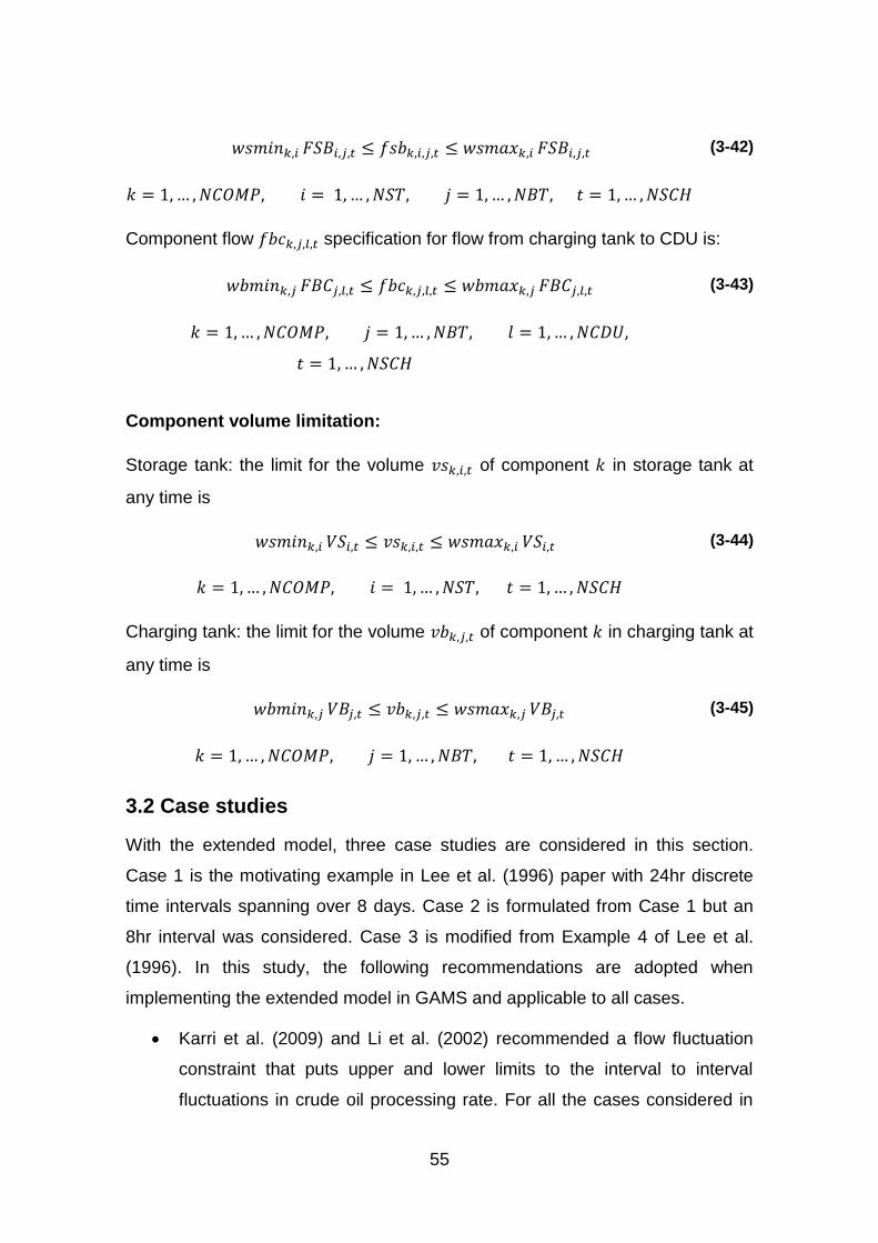
55

𝑤𝑠𝑚𝑖𝑛𝑘,𝑖 𝐹𝑆𝐵𝑖,𝑗,𝑡 ≤ 𝑓𝑠𝑏𝑘,𝑖,𝑗,𝑡 ≤ 𝑤𝑠𝑚𝑎𝑥𝑘,𝑖 𝐹𝑆𝐵𝑖,𝑗,𝑡

𝑘 = 1,… ,𝑁𝐶𝑂𝑀𝑃, 𝑖 = 1, … ,𝑁𝑆𝑇, 𝑗 = 1,… ,𝑁𝐵𝑇, 𝑡 = 1,… ,𝑁𝑆𝐶𝐻

(3-42)

Component flow 𝑓𝑏𝑐𝑘,𝑗,𝑙,𝑡 specification for flow from charging tank to CDU is:

𝑤𝑏𝑚𝑖𝑛𝑘,𝑗 𝐹𝐵𝐶𝑗,𝑙,𝑡 ≤ 𝑓𝑏𝑐𝑘,𝑗,𝑙,𝑡 ≤ 𝑤𝑏𝑚𝑎𝑥𝑘,𝑗 𝐹𝐵𝐶𝑗,𝑙,𝑡

𝑘 = 1,… ,𝑁𝐶𝑂𝑀𝑃, 𝑗 = 1,… ,𝑁𝐵𝑇, 𝑙 = 1,… ,𝑁𝐶𝐷𝑈,

𝑡 = 1,… ,𝑁𝑆𝐶𝐻

(3-43)

Component volume limitation:

Storage tank: the limit for the volume 𝑣𝑠𝑘,𝑖,𝑡 of component 𝑘 in storage tank at

any time is

𝑤𝑠𝑚𝑖𝑛𝑘,𝑖 𝑉𝑆𝑖,𝑡 ≤ 𝑣𝑠𝑘,𝑖,𝑡 ≤ 𝑤𝑠𝑚𝑎𝑥𝑘,𝑖 𝑉𝑆𝑖,𝑡

𝑘 = 1,… ,𝑁𝐶𝑂𝑀𝑃, 𝑖 = 1, … ,𝑁𝑆𝑇, 𝑡 = 1, … , 𝑁𝑆𝐶𝐻

(3-44)

Charging tank: the limit for the volume 𝑣𝑏𝑘,𝑗,𝑡 of component 𝑘 in charging tank at

any time is

𝑤𝑏𝑚𝑖𝑛𝑘,𝑗 𝑉𝐵𝑗,𝑡 ≤ 𝑣𝑏𝑘,𝑗,𝑡 ≤ 𝑤𝑠𝑚𝑎𝑥𝑘,𝑗 𝑉𝐵𝑗,𝑡

𝑘 = 1,… , 𝑁𝐶𝑂𝑀𝑃, 𝑗 = 1, … , 𝑁𝐵𝑇, 𝑡 = 1, … , 𝑁𝑆𝐶𝐻

(3-45)

3.2 Case studies

With the extended model, three case studies are considered in this section.

Case 1 is the motivating example in Lee et al. (1996) paper with 24hr discrete

time intervals spanning over 8 days. Case 2 is formulated from Case 1 but an

8hr interval was considered. Case 3 is modified from Example 4 of Lee et al.

(1996). In this study, the following recommendations are adopted when

implementing the extended model in GAMS and applicable to all cases.

Karri et al. (2009) and Li et al. (2002) recommended a flow fluctuation

constraint that puts upper and lower limits to the interval to interval

fluctuations in crude oil processing rate. For all the cases considered in

56

this study, a ceiling of 10% is fixed for flow variation while at the same

time restricting the CDUs to run within the permissible minimum

turndown ratio of 10:6.

In consideration to the manner in which storage and charging tanks are

configured as floating roof objects in a refinery and the volatile nature of

crude oil, a minimum level of the fluid is always maintained in those tanks

for safety reasons. This work suggests that a minimum level for all tanks

be fixed at 100kbbl and a maximum value at 1100kbbl. The difference

between these two values is in agreement with the volume difference

used in Lee et al. (1996).

3.2.1 Case 1

The case study begins with the motivating example from the Lee et al. (1996) to

illustrate how the ideas proposed in this work help in achieving better and

realistic results. Like in Lee et al. (1996), this work considered a system with

one docking station, two crude vessels (V1 and V2), two storage tanks (ST1

and ST2), two charging tanks (CT1 and CT2) and one CDU. The flow network is

shown in Figure 3-1. As shown in Table 3-1, V1 and V2 arrive for unloading into

the storage tanks on day 1 and day 5 respectively. In the table, other detailed

information required for solving this problem is provided (Yüzgeç et al., 2010).

Vessels storage tanks charging tanks CDU

Figure 3-1: Flow network diagram for Case 1 (Lee et al., 1996)

The extended model was implemented in GAMS v 23.9.1 on a 4GB RAM dual

core i5 processor computer, using the CPLEX solver. The optimal operating

cost of processing 2.0Mbbl of crude in charging tanks was obtained in 0.765

57

seconds as $216,425 after 1287 iterations in 35 nodes. It consists of $150,000

changeover cost, $58,000 unloading and sea waiting cost and $8,425 inventory

cost. The optimal schedule generated for the problem is represented in Figure

3-2.

Table 3-1: System information for Case 1 (Yüzgeç et al., 2010)

Scheduling horizon(days) 8

Time interval (hour) 24

Number of vessels 2

Number of storage tanks 2

Number of charging tanks 2

Number of CDU 1

Crude vessels Arrive/depart Volume of crude Key component

V1 1st day/5th day 1,000,000 bbl 0.01

V2 5th day/8th day 1,000,000 bbl 0.06

Storage Tanks Capacities Initial volume Key component

ST1 1,100,000 bbl 250,000 bbl 0.01

ST2 1,100,000 bbl 750,000 bbl 0.06

Charging Tanks Capacities Initial volume Initial(min., max)

CT1 1,100,000 bbl 500,000 bbl 0.02(0.015-0.025)

CT2 1,100,000 bbl 500,000 bbl 0.05(0.045-0.055)

Vessel unloading cost [$/day] 8,000

Sea waiting cost [$/day] 5,000

Storage tank inventory unit cost [$/(day x

bbl)]

0.005

Charging tank inventory unit cost [$/(day x

bbl)]

0.008

Unit changeover cost for charged oil switch in

CDU[$]

50,000

Demand of crude mix from charging tanks to CDU for the whole scheduling horizon

Blend 1 1,000,000 bbl

Blend 2 1,000,000 bbl

Flow constraints Minimum(bbl/day) Maximum(bbl/day)

Flow from vessel to storage tank 0 500,000

Flow from storage tank to charging tank 0 500,000

Flow from charging tank to CDU 50,000 500,000

58

(a)

Task Operation Scheduling horizon (days)

1 2 3 4 5 6 7 8

Unloading

1 V1-ST1

2 V2-ST2

Transfers

3 ST1-CT1

4 ST1-CT2

5 ST2-CT1

6 ST2-CT2

Distillation

7 CT1-CDU1

8 CT2-CDU1

(b)

Figure 3-2: Optimal schedule for Case 1

From the schedule shown in Figures 3-2(a) and 3-2(b), V1 arrives on the first

day as determined at the planning level but unloading was delayed until the

second day because the standing gauge operation forbids the vessel from

unloading (since ST1 was busy on that day, transferring crude to CT2). This V1

unloads only 500,000bbl of crude oil on the second day and the remaining

500,000bbl on the third day. Unloading on the first day will amount to a savings

of $5,000 of sea waiting cost but will increase the inventory levels of the storage

and charging tanks incurring an additional switchover cost of $50,000. This is

due to the fact that increase in the inventory level of storage tank implies an

increase in the charging tank inventory level which will ultimately increase the

59

charging tank switch over frequency. For the same reason as V1, V2 equally

arrives on the fifth day but does not begin unloading until the sixth day. V2

unloads 500,000bbl on the sixth day and the remaining 500,000bbl on the

seventh day. Furthermore, V2 cannot unload earlier than the sixth day because

ST2 was busy transferring crude oil to CT1 on the fourth and the fifth days and

cannot transfer crude oil to ST1 as this tank is dedicated to receive crude oil

only from the V1.

Transfers from storage to charging tanks also happen only when the charging

tanks are not charging the CDU. ST1 transfers to CT1 only on days 4 and 5 and

to CT2 only on the first day because these tanks do not charge the CDU on

these days as shown in Figure 3-2(b). ST1 is actually transferring to CT2 on the

first day from its initial inventory level of 250,000bbl (Table 3-1) since V1 starts

unloading after day 1. Plots of volume variation in the storage and charging

tanks are presented in Figures 3-3 and 3-4. From the figures, the inventory level

in the storage tanks goes up at the end of the horizon, while that of the charging

tanks is kept as minimal as possible because the charging tanks inventory cost

is higher than storage tanks inventory cost.

Figure 3-3: Optimal volume variations in storage tanks

Figure 3-3 shows that the required minimum tank level of 100,000bbl was

maintained and flow from the vessel to the storage tank was actually accounted

0

20

40

60

80

100

120

0 1 2 3 4 5 6 7 8

Vo

lum

e [

bb

l x 1

0,0

00

]

Time interval (days) Storage tank 1

Storage tank 2

60

for by an equivalent rise in the storage tank level during and immediately after

the period that the vessel unloaded to the storage tank. For example a

1,100,000 bbl rise in volume level in ST1 occurs on the fourth day, which is

exactly one day after V1 finishes unloading into ST1. Armed with the

information that the V2 will arrive on day 5, ST2 is scheduled to quickly unload

its content down to the minimum volume from day 1 until day 6 so that it can

receive from V2 rights from that day 6 to minimize sea waiting cost. ST2 took a

longer period of more than 5 days to reach the minimum tank level because its

initial inventory level is higher (Table 3-1).

Figure 3-4: Optimal volume variations in charging tanks

In Figure 3-4, CT1 transfers 200,000bbl of blended crude oil 1 to the CDU from

day 1 to day 2 then another 200,000bbl of the same blended crude oil until the

tank reaches its minimum level at day 3 after which tank switchover occurs so

that it can be loaded while CT2 charges the CDU. During the period that CT2

feeds the CDU, CT1 receives a total of 100,000bbl on day 4 from ST1 and ST2

and a total of 500,000bbl on day 5 from the same storage tanks to prepare a

blend for days 7 and 8. A total of two changeovers are recorded in this case

study.

Changeover is expensive because it poses a big disturbance to the CDU but

cannot be altogether avoided. In an attempt to minimize the changeover

0

20

40

60

80

100

120

0 1 2 3 4 5 6 7 8

Vo

lum

e [

bb

l x 1

0,0

00

]

Time interval (days)

Charging tank 1

Charging tank 2

61

frequency at all cost, an unrealistic and sudden drop in CDU charge rate are

reported in some instances in Lee et al. (1996) paper. This sudden change can

leads to the production of cut fractions with low quality in terms of component

separation. In this study a flow fluctuation constraint is introduced, which

determines the interval to interval fluctuation of the CDU charge rate. The

changeover cost computed using the original model is $100,000 against

$150,000 for the extended model. The benefit of including interval to interval

constraint in the extended model is therefore assessed not in terms of cost but

in its ability to ensure that CDU charging rate is within the acceptable limits.

In Figure 3-5, the CDU charging schedule for the extended model has shown

that the CDU charging rate is in the range of 200,000bbl to 300,000bbl

throughout the 8 day period, a huge difference from the original model where

fluctuation in CDU charge rate exceeded 100% in one instance. The CDU

charging is also within the permissible minimum turndown ratio of 10:6. At the

end of the horizon, the total quantity of blended crude oil 1 and 2 actually

matches demand for each.

Figure 3-5: Optimal CDU charging schedule

Figure 3-6 represents the concentration of the key component (sulphur) in

charging tanks. A plot of concentrations of sulphur in CT1 and CT2 in Figure 3-6

clearly indicates that in the course of the blending operations, the sulphur level

0

5

10

15

20

25

30

35

1 2 3 4 5 6 7 8

Vo

lum

e [

bb

l x 1

0,0

00

]


Crude mix 1 Crude mix 2

62

for both tanks did not exceed their maximum levels specified. Ideally, the

variation of sulphur concentration in tanks should be constant on days when

there is no transfer of crude oil into the tanks. However, a minor discrepancy is

noted here, for example, in CT1, the sulphur concentrations are 0.020 vol/vol

and 0.017 vol/vol on days 1 and 2 respectively. This discrepancy is due to the

linearized bilinear equation used to avoid non-linearity in the model. Despite this

discrepancy, the maximum level of sulphur was not exceeded in the charging

tanks.

Figure 3-6: Optimal variation in concentration of sulphur

3.2.2 Case 2

This case is same as Case 1 except that the horizon further splits into 8-hour

time interval. An 8-hour time period is chosen because a typical refinery

operates based on 8-hr shift. The total operating cost of $199,460 was obtained

after 17,630 iterations using 247 nodes in 2.380 seconds. The 8-hour schedule

results in a difference of $16,965 compared to the 24-hr schedule (Case 1). The

vessel unloading schedule for the two cases shows a slight difference as V1

and V2 starts unloading earlier in Case 2. Table 3-2 shows a comparison

between the various costs incurred for Cases 1 and 2 and the optimal schedule

for both cases is presented in Figure 3-7.

0

0.01

0.02

0.03

0.04

0.05

0.06

0 1 2 3 4 5 6 7 8

Co

nc.

of

sulp

hu

r (v

ol/

vol )


Charging tank 1Charging tank 2

63

Table 3-2: Comparison between optimal cost for Cases 1 and 2

Cost Case 1(24-hr period) Case 2 (8-hr period)

Sea waiting cost ($) 10,000 0

Unloading cost ($) 48,000 40,050

Storage tank inventory cost

($)

3,358 4,630

Charging tank inventory

cost ($)

5,067 4,780

Changeover cost ($) 150,000 150,000

Operating cost ($) 216,425 199,460

Case Task Scheduling horizon (days)

1 2 3 4 5 6 7 8

Unloading

1 1

1 2

2 1

2 2

Transfers

1 1

1 2

1 3

1 4

2 1

2 2

2 3

2 4

Distillation

1 1

1 2

2 1

2 2

Figure 3-7: Comparison of optimal schedule for Cases 1 and 2

It is obvious from Figure 3-7 that the two vessels starts unloading on the actual

days determined at the planning level incurring no sea waiting costs. V1 has to

stop unloading after 8hr of the first day in order for ST1 to transfer crude to CT2.

This decision would have been hidden if 24hr time period is adopted as it

basically reveals information from day to day without exploring other events

happening within the day. For discrete-time representation, using smaller time

intervals creates more decision points, giving the model more flexibility in

searching for optimal values for the decision variables. For example the first

changeover operation in Case 1 could be assumed to have taken place at the

end of the second day which is not true. The second changeover operation is

equally delayed to the end of sixth day implying that the CDU may not have a

64

sufficient amount of blended crude oil to sustain it on the seventh day. The two

cases recorded the same number of changeover operations. The inventory

levels are also compared and presented in Figure 3-8 and Figure 3-9.

Since storage inventory cost depends on both the quantity and time of storage,

it is a direct function of the area bounded by the curve and the two axes. In

Figure 3-8, volume variation for both the 24-hr and 8-hr curves have shown a

shrinking of these areas to minimize the inventory cost. The 24-hr (Case 1)

period however shows a better shrinking of this area by having steeper slopes

than the 8-hr (Case 2) period. ST1 in both cases has almost the same quantity

of crude oil on the sixth day and maintains this volume up to the end of the

scheduling horizon. For ST2, Case 1 has the lower inventory level reaching the

minimum amount on day 6 before raising again to a level same as Case 2 at the

end of the horizon. This accounts for lower inventory cost of Case 1 compared

to Case 2.

Figure 3-8: Optimal volume variations in storage tanks for Case 1 and Case 2

0

20

40

60

80

100

120

0 1 2 3 4 5 6 7 8

Vo

lum

e [

bb

l x 1

0,0

00

]


Storage tank 1 (Case 1)Storage tank 2 (Case 1)Storage tank 1 (Case 2)Storage tank 2 (Case 2)

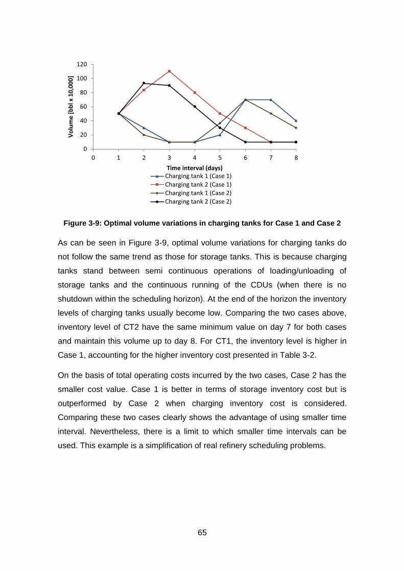
65

Figure 3-9: Optimal volume variations in charging tanks for Case 1 and Case 2

As can be seen in Figure 3-9, optimal volume variations for charging tanks do

not follow the same trend as those for storage tanks. This is because charging

tanks stand between semi continuous operations of loading/unloading of

storage tanks and the continuous running of the CDUs (when there is no

shutdown within the scheduling horizon). At the end of the horizon the inventory

levels of charging tanks usually become low. Comparing the two cases above,

inventory level of CT2 have the same minimum value on day 7 for both cases

and maintain this volume up to day 8. For CT1, the inventory level is higher in

Case 1, accounting for the higher inventory cost presented in Table 3-2.

On the basis of total operating costs incurred by the two cases, Case 2 has the

smaller cost value. Case 1 is better in terms of storage inventory cost but is

outperformed by Case 2 when charging inventory cost is considered.

Comparing these two cases clearly shows the advantage of using smaller time

interval. Nevertheless, there is a limit to which smaller time intervals can be

used. This example is a simplification of real refinery scheduling problems.

0

20

40

60

80

100

120

0 1 2 3 4 5 6 7 8

Vo

lum

e [

bb

l x 1

0,0

00

]

Time interval (days) Charging tank 1 (Case 1)

Charging tank 2 (Case 1)



66

3.2.3 Case 3

Case discussed in this section considers typical industrial issues faced in real

life. Besides, the size of the problem has been extended to accommodate more

resources. The features below were considered in the extended model.

Closing stocks are fixed to avoid low inventory at the end of the

scheduling horizon.

A setup penalty for tank-tank is introduced and added to the objective

function to deter unnecessary switching when storage tank transfer crude

oil into charging tank.

Shutdown constraint is made active to generate schedule that is immune

to CDU disruption during execution in the real plant.

The system consists of a docking station, three vessels, six storage tanks, four

charging tanks and three CDUs. System information is obtained from Lee et al.

(1996) with slight modifications on the charging tanks’ minimum and maximum

capacities and is presented in Table 3-3.

In this study, the setup penalty included in the objective function is chosen

based on the importance of the tanks transfer operations relative to two other

critical operations namely shutdown operation and charging tanks switching

operations. These two operations cannot be compromised while trying to avoid

tank-tank transfers. Also the CDU cannot be shut down in an effort to prevent

frequent changeover operations.

Based on this, a setup cost for tank-tank transfer much less than the

changeover cost is used. A figure is selected so that the total setup cost at any

time does not exceed the cost of a changeover operation. For this Case a

conservative cost of $500 per setup operation is used. Figure 3-10(a) compares

the tank-tank transfer operations with and without the set-up penalty and Figure

3-10(b) presents the flow network.

67

Table 3-3: System information for Case 3 (Lee et al., 1996)


Vessels Arrive/depart Volume of crude Key component

V1 1st /6th 600,000 bbl 0.03

V2 6th /11th 600,000 bbl 0.05

V3 11th /15th 600,000 bbl 0.065

Storage Tanks

Capacities Initial volume(bbl) Key component Initial(min, max) Min. Max.

ST1 100,000bbl 900,000bbl 600,000 0.031(0.025-0.038)

ST2 100,000bbl 1,100,000bbl 100,000 0.03(0.02-0.04)

ST3 100,000bbl 1,100,000bbl 500,000 0.05(0.04-0.06)

ST4 100,000bbl 1,100,000bbl 400,000 0.065(0.06-0.07)

ST5 100,000bbl 900,000bbl 300,000 0.075(0.07-0.078)

ST6 100,000bbl 900,000bbl 600,000 0.075(0.07-0.078) Charging

Tanks Capacities Initial volume(bbl) Key component

Initial(min, max) Min. Max.

CT1 100,000bbl 1,100,000bbl 50,000 bbl 0.0317(0.03-0.035)

CT2 100,000bbl 1,100,000bbl 300,000 bbl 0.0483(0.043-0.05)

CT3 100,000bbl 1,100,000bbl 300,000 bbl 0.0633(0.06-0.065)

CT4 50,000bbl 850,000bbl 300,000 bbl 0.075(0.071-0.08)



Storage tank inventory unit cost [$/(day x bbl)]

0.005

Charging tank inventory unit cost [$/(day x bbl)]

0.006

Unit changeover cost for charged oil switch in CDU[$]

30,000

Tank-tank setup cost [$/setup] 500

Demand of crude mix from charging tanks to CDU for the whole scheduling period

Blend 1 600,000 bbl

Blend 2 600,000 bbl

Blend 3 600,000 bbl

Blend 4 600,000 bbl

In each situation a total of 1,500,000bbl of crude has been transferred from

storage tanks to charging tanks in the scheduling horizon. When set-up penalty

is included, the number of tanks transfer tasks decreased from 8 to 7 even

though the same amount of crude oil has been transferred. This is because less

critical activities were merged into a single activity to cut down setup cost. For

every task represented by the blue strips in Figure 3-10(a), two sets of

operations are performed at the boundaries of the intervals: one operation at

the beginning and another one at the end. Without a tank-tank setup penalty,

there are 8 tasks involving 16 operations. Adding such penalty reduces the

68

number of operations from 16 to 14, which is over 12% slash in the number of

operations required.


1 2 3 4 5 6 7 8 9 10 11 12 13 14 15

Tank-tank transfer with set-up penalty (bbl x 10,000)

1 ST1-CT1 5, 25

2 ST2-CT1 25

4 ST3-CT2 25 5

5 ST3-CT3 7

7 ST4-CT3 25

8 ST5-CT3 3

10 ST6-CT4 5, 25

Tank-tank transfer without set-up penalty (bbl x 10,000)

1 ST1-CT1 10, 25

2 ST2-CT1 25

3 ST2-CT2 14.714

4 ST3-CT2 5

5 ST3-CT3 6.667 6.667

6 ST4-CT2 10.286

7 ST4-CT3 3.333 13.333

10 ST6-CT4 5, 25

(a)

(b)

Figure 3-10: Optimal tank-tank schedule

69

This case involves a small amount as penalty for tank-tank switching and as the

magnitude of this penalty is made to be larger, more operations that are not

critical to the tank transfer will be cut down. The optimal schedule with set-up

cost is presented in Figure 3-11.


1 2 3 4 5 6 7 8 9 10 11 12 13 14 15

Unloading

1 V1-ST2

2 V2-ST3

3 V3-ST4

Transfers

1 ST1-CT1

2 ST2-CT1

4 ST3-CT2

5 ST3-CT3

7 ST4-CT3

8 ST5-CT3

10 ST6-CT4

Distillation

1 CT1-CDU1

2 CT2-CDU1

3 CT2-CDU2

4 CT3-CDU2

5 CT3-CDU3

6 CT4-CDU3

Figure 3-11: Optimal schedule (with set up cost) for Case 3

The proposed formulation is solved in 16.29 seconds using 1391 nodes. Total

operating cost for this case is $ 360,867 lower than example 4 of Lee et al.

(1996) optimal cost ($420,999). The cost reduction is due to the cost penalty for

tank-tank transfer and sea waiting cost was not incurred as vessel unloading

was not delayed. The effort here is not focussed on comparing with Lee et al.

(1996) because their work does not include a set-up penalty for tank-tank

transfer and uses different limits for storage and charging tanks safety stocks.

Rather, the focus here is to draw attention to the need to include a setup

penalty each time a tank-tank transfer operation occurs.

Figure 3-12 shows the optimal volume variation for the storage tanks.

Understandably the inventory levels in the storage tanks are kept higher than

charging tanks due to the fact that charging tanks are transferring mixed crude

oil to CDU as soon as the blends are processed to satisfy the CDU demand

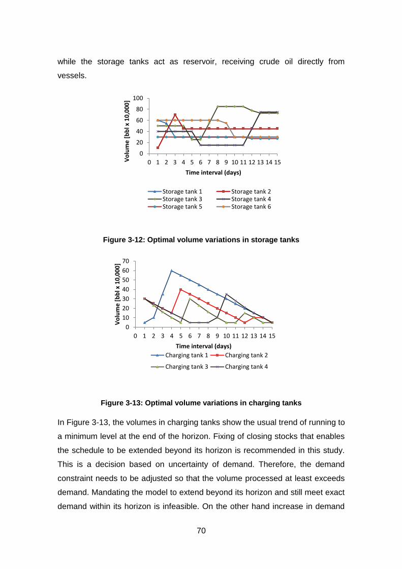
70

while the storage tanks act as reservoir, receiving crude oil directly from

vessels.

Figure 3-12: Optimal volume variations in storage tanks

Figure 3-13: Optimal volume variations in charging tanks

In Figure 3-13, the volumes in charging tanks show the usual trend of running to

a minimum level at the end of the horizon. Fixing of closing stocks that enables

the schedule to be extended beyond its horizon is recommended in this study.

This is a decision based on uncertainty of demand. Therefore, the demand

constraint needs to be adjusted so that the volume processed at least exceeds

demand. Mandating the model to extend beyond its horizon and still meet exact

demand within its horizon is infeasible. On the other hand increase in demand

0

20

40

60

80

100

0 1 2 3 4 5 6 7 8 9 10 11 12 13 14 15Vo

lum

e [

bb

l x 1

0,0

00

]


Storage tank 1 Storage tank 2Storage tank 3 Storage tank 4Storage tank 5 Storage tank 6

0

10

20

30

40

50

60

70

0 1 2 3 4 5 6 7 8 9 10 11 12 13 14 15

Vo

lum

e [

bb

l x 1

0,0

00

]


Charging tank 1 Charging tank 2

Charging tank 3 Charging tank 4

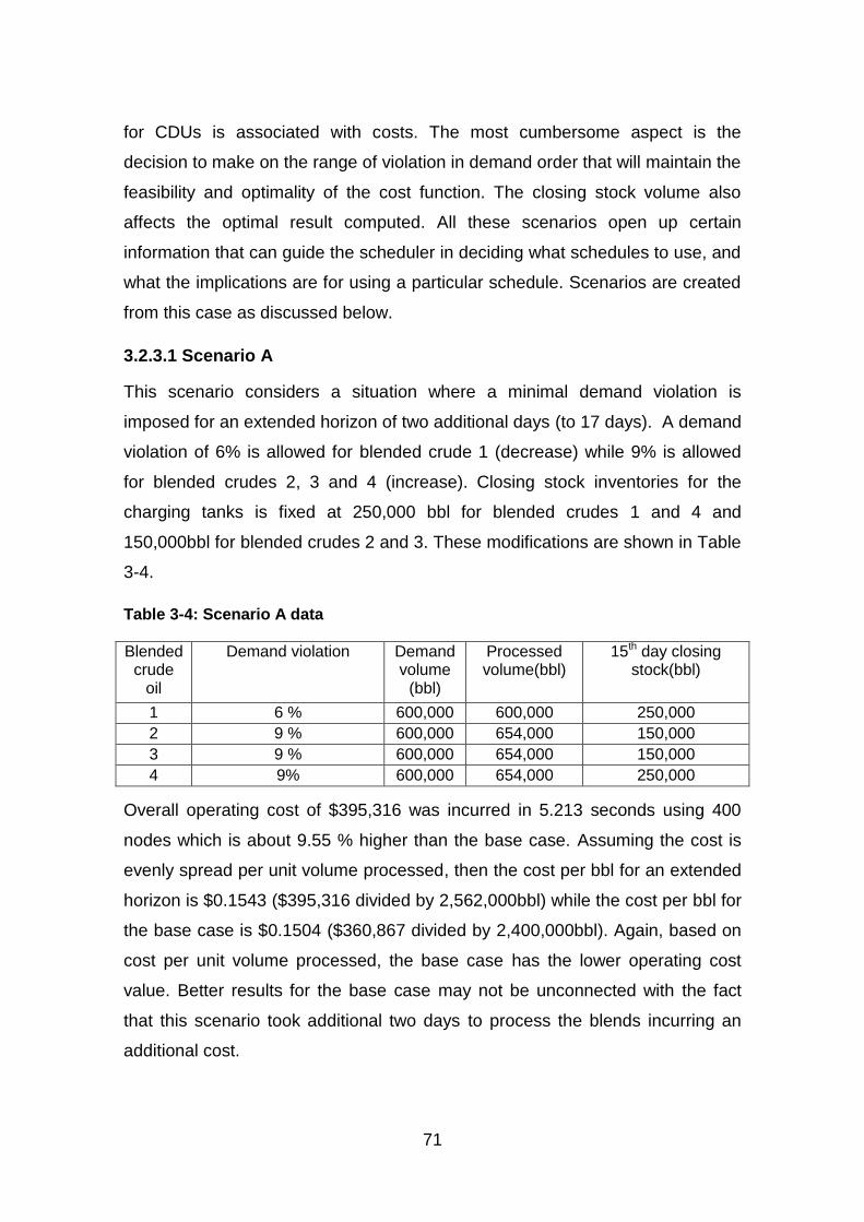
71

for CDUs is associated with costs. The most cumbersome aspect is the

decision to make on the range of violation in demand order that will maintain the

feasibility and optimality of the cost function. The closing stock volume also

affects the optimal result computed. All these scenarios open up certain

information that can guide the scheduler in deciding what schedules to use, and

what the implications are for using a particular schedule. Scenarios are created

from this case as discussed below.

3.2.3.1 Scenario A

This scenario considers a situation where a minimal demand violation is

imposed for an extended horizon of two additional days (to 17 days). A demand

violation of 6% is allowed for blended crude 1 (decrease) while 9% is allowed

for blended crudes 2, 3 and 4 (increase). Closing stock inventories for the

charging tanks is fixed at 250,000 bbl for blended crudes 1 and 4 and

150,000bbl for blended crudes 2 and 3. These modifications are shown in Table

3-4.

Table 3-4: Scenario A data

Blended crude

oil

Demand violation Demand volume

(bbl)

Processed volume(bbl)

15th day closing stock(bbl)

1 6 % 600,000 bbl

600,000 250,000

2 9 % 600,000 bbl

654,000 150,000

3 9 % 600,000 bbl

654,000 150,000

4 9% 600,000 bbl

654,000 250,000

Overall operating cost of $395,316 was incurred in 5.213 seconds using 400

nodes which is about 9.55 % higher than the base case. Assuming the cost is

evenly spread per unit volume processed, then the cost per bbl for an extended

horizon is $0.1543 ($395,316 divided by 2,562,000bbl) while the cost per bbl for

the base case is $0.1504 ($360,867 divided by 2,400,000bbl). Again, based on

cost per unit volume processed, the base case has the lower operating cost

value. Better results for the base case may not be unconnected with the fact

that this scenario took additional two days to process the blends incurring an

additional cost.

72

Because of the demand violation, quantity of blended crude 1 meets exact

demand, while blended crudes 2, 3 and 4 were above demand. The quantity of

blended crude 1 processed meet exact demand even when violation of 6% is

allowed; this is because the extended model is more sensitive to the increase in

demand order. Demand violation of 6% up to 88% for blended crude 1 does not

change the optimal operating cost. However, with violation above 88% the

operating cost assumed a different value. Violation in demand of blended crude

2, 3 or 4 below 9% generates infeasible solution.

3.2.3.2 Scenario B

Here demand violation for all the crude mixes are allowed so that all the CDUs

process above demand. When the same closing stock for scenario A was used

the model was infeasible because of insufficient stock in the charging tanks.

The 15th day closing stocks for these tanks were increased as in Table 3-5.

Table 3-5: Scenario B data

Blended crude oil Demand volume (bbl)

Processed volume (bbl)

15th day closing stock (bbl)

1 600,000 620,000 300,000

2 600,000 654,000 200,000

3 600,000 650,000 150,000

4 600,000 654,000 250,000

The operating cost is $394,500 generated in 28.892 seconds using 2640 nodes.

It is obvious from the results that scenario B is more cost effective as compared

with scenario A. This can be verified further by comparing total operating cost

with the volume processed. In scenario A, a total of 2,562,000bbl was

processed at a cost of $395,316 which is about $0.1543 per barrel. Scenario B

handles 2,578,000bbl at a cost of $394,500 which is about $0.1530 per barrel.

Comparing just the operating costs for the two scenarios, scenario B involves a

smaller operating cost. Also, when the cost per barrel is compared, scenario B

is still a better option to go by.

3.2.3.3 Scenario C

In the preceding scenarios and the base case, schedules are generated while

all the three CDUs are in operation. In some circumstances one CDU may not

73

be operated due to maintenance or breakdown and schedules can still be

generated with the available CDUs at an extra cost. In this scenario a disruption

is introduced such that one of the CDUs is shut down. This will enable

generating a schedule that anticipates no operation of CDU 2. All the blended

crudes have to be processed by CDUs 1 and 3. A demand violation of 5% is

allowed for blended crudes 1 and 4 while 7% is allowed for blended crudes 2

and 3. Closing stock inventories for the charging tanks are fixed at 200,000 bbl

for blended crudes 1 and 4 and 50,000bbl for blended crudes 2 and 3. This

generates schedule at the cost of $474,747. There is no cost comparison with

the preceding scenarios because shutdown results in an additional cost. The

schedule is shown in Figure 3-14.

Operation Scheduling horizon

1 2 3 4 5 6 7 8 9 10 11 12 13 14 15 16 17

Distillation CDU 1

CT1-CDU1

CT2-CDU1

CDU 3

CT3-CDU3

CT4-CDU3

Figure 3-14: Optimal CDU schedules for Scenario C

3.3 Summary of contributions in this chapter

Below is the highlight of the contributions in this chapter. Here, the following

constraints are included to come up with a more reliable MILP short-term

scheduling model addressing real life refinery operational issues.

Flow fluctuation constraints: These are added to prevent interval-interval

variation of CDU charging rates. The constraints are enforced using

Equations 3-18 and 3-19. These constraints were not included in Lee et

al. (1996) and as a result schedules generated using their model

produced unrealistic widely fluctuating CDU charging rate.

CDU shutdown constraints with penalty: Because of the huge losses

associated with shutdown, it is highly undesirable and plants are for most

times run continuously. However, uncertainty due to disruption cannot be

74

avoided altogether. This study therefore considers constraints that allow

generating schedules even when not all the CDUs are in operation. The

constraints are represented by Equations 3-23 and 3-24. A shutdown

penalty is included in the objective function to minimize any cost

associated with the shutdown operation.

Set-up constraint (Equation 3-25) with penalty: This is to optimize the

number of activities prior to transfer from storage tanks to charging tanks

for a case involving unloading into multiple storage tanks and

subsequent transfer of crude oil into multiple charging tanks. The

extended model schedules only important set-ups thereby minimizing the

number of operations during tank-tank transfers when a set-up penalty is

included in the objective function. This set-up constraint with penalty is

considered in Case 3.

Demand violation constraints: Unlike in Lee et al. (1996), violations in

demand order are introduced here to make the model more flexible.

These are necessary because the model becomes infeasible where

supply failed to meet exact demand. These are represented by

Equations 3-15 and 3-16 and incorporated in Case 3.

Standing gauge constraints are applied not only when charging tank

feeds CDU but also during transfer from storage tanks to charging tanks

(Equations 3-10 and 3-11). This is an industry practice which was not

included in Lee et al. (1996).

75

4 CRUDE OIL SCHEDULING UNDER CDU DEMAND

UNCERTAINTY

4.1 Receding Horizon Approach

In the preceding chapter, uncertainties due to crude distillation unit (CDU)

disruption and low inventory in charging tanks are dealt with using some

constraints while fixing closing stocks. An improvement to this procedure is to

generate more reliable schedules with periodic update to keep track for

changes in process conditions, constraints, or performance criteria. A control

technique usually refers to as model predictive control (MPC) is an alternative

that keeps the decision variables at the required values (set points) while

generating an optimal schedule. A key feature of this control strategy is that

current implementation of decision variables within the scheduling horizon can

be done more accurately since the process is periodically updated. One form of

MPC is a rolling or receding horizon; a strategy that allows repeated

calculations and predictions updated based on the current value of decision

variable.

In this chapter, scheduling problem of crude oil transfer, blending and CDU

charging has been formulated under the framework of receding horizon control

strategy. The extended model developed in the previous chapter is adopted.

The model considers a refinery receiving crude oil from vessels via pipeline;

storing the crude oil in tanks and transferring the crude oil to charging tanks

where blending operation is carried out. The blended crude oils are transferred

to CDUs in accordance with the CDUs crude oil quality requirements.


Given all the necessary information about the crude parcel, unit facilities, length

of scheduling horizon, stream connections, CDU mixed crude oil requirements

and the extended model, the task is to recommend to a refinery operator the

feasible and smooth operational procedures that guarantee performance at

minimum cost even in the presence of uncertainty (disturbance).

76

4.1.2 Methodology

Receding horizon is a strategy based on obtaining outputs or current state of a

system and predicting subsequent future outputs or states using previous states

of the system. The algorithm is made up of two elements: a prediction model of

the system and the optimization tool (Yüzgeç et al., 2010).

The set of future decisions are computed by the optimization tool according to

the constraints and cost function. The optimization problem is solved over a

certain horizon length where a sequence of decision variables are determined

for a number of time steps and then implementing only the first step in the

series. This is achieved using the prediction model where a set of decisions are

obtained and optimized for implementation in a real plant. The time then moves

by one step with the information from the preceding time step used as input and

the process is repeated until the last step. The difference between two time

steps is given by the sampling time chosen (Goodwin et al., 2006).

Based on the prediction horizon length, receding horizon strategy can be fixed-

end (where the prediction length is varying) or moving-end (in which the length

is constant). In the fixed end receding horizon presented in this work, the length

is decreasing when moving from one time step to the next as shown in Figure 4-

1. Moving end receding horizon presented in Figure 4-2 here follows similar

solution procedure in Yüzgeç et al. (2010).

Figure 4-1: Fixed end receding horizon

77

Figure 4-2: Moving end receding horizon

In this work, crude oil scheduling problem involving crude oil unloading,

blending and CDU charging is solved over the fixed end and moving end

receding horizon strategies. The key advantage of the strategies is that they

accommodate new information or uncertain parameters (disturbance) such as

change in demand of blended crude by CDU within the scheduling horizon.

Without disturbance, the states of the system using receding horizon strategies

will be approximately close to those obtainable using the traditional approach.

The strategy presented in this study (fixed end) was compared with the

traditional approach and then with another strategy (moving end) using Case 1

and Case 2. Some disturbance scenarios were introduced to evaluate the

performances of fixed end and moving end horizon strategies for

recommendation to refiners and process operators.

4.2 Case Studies

The crude oil scheduling model discussed earlier was implemented in GAMS v

23.9.1 on a 4GB RAM dual core i5 processor computer, using the CPLEX

solver. Case 1 and Case 2 are considered in this study to evaluate the

performance of the receding horizon strategies. Some of the constraints in

Chapter 3 are not applicable here and thus excluded from the optimization

model. For example, shutdown is not allowed as all the CDUs should be in

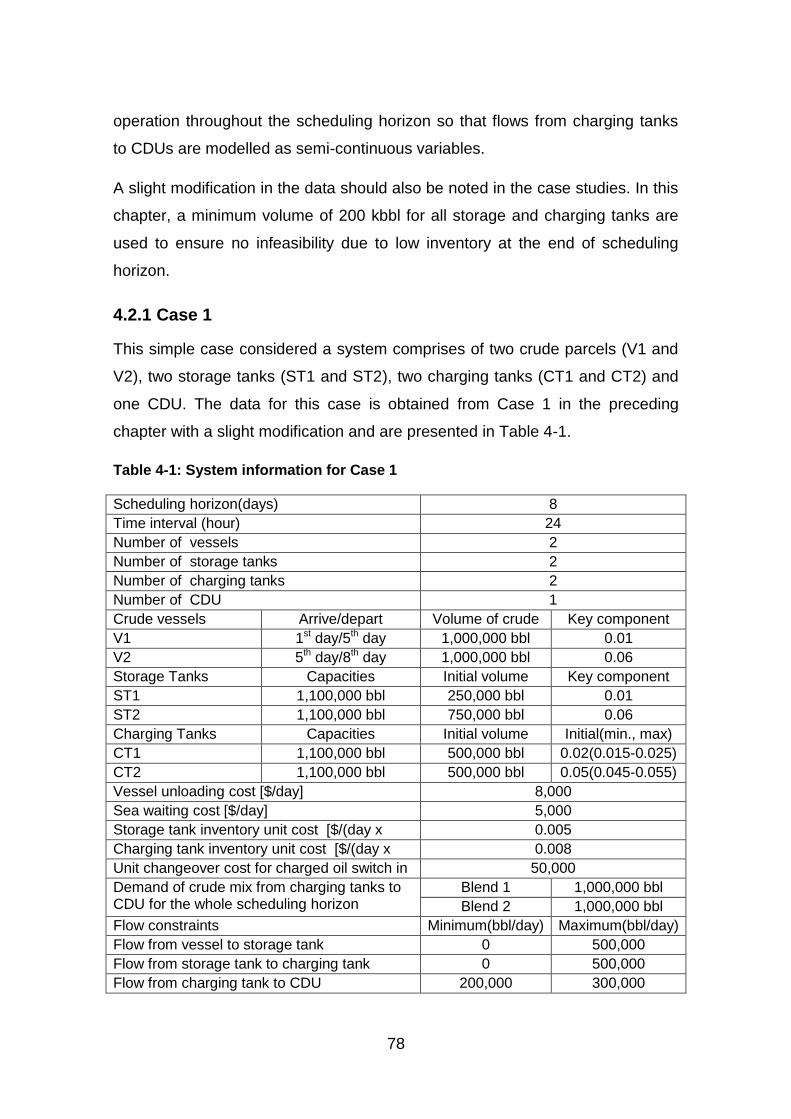
78

operation throughout the scheduling horizon so that flows from charging tanks

to CDUs are modelled as semi-continuous variables.

A slight modification in the data should also be noted in the case studies. In this

chapter, a minimum volume of 200 kbbl for all storage and charging tanks are

used to ensure no infeasibility due to low inventory at the end of scheduling

horizon.

4.2.1 Case 1

This simple case considered a system comprises of two crude parcels (V1 and

V2), two storage tanks (ST1 and ST2), two charging tanks (CT1 and CT2) and

one CDU. The data for this case is obtained from Case 1 in the preceding

chapter with a slight modification and are presented in Table 4-1.

Table 4-1: System information for Case 1


Time interval (hour) 24

Number of vessels 2

Number of storage tanks 2

Number of charging tanks 2

Number of CDU 1

Crude vessels Arrive/depart Volume of crude Key component

V1 1st day/5th day 1,000,000 bbl 0.01

V2 5th day/8th day 1,000,000 bbl 0.06

Storage Tanks Capacities Initial volume Key component

ST1 1,100,000 bbl 250,000 bbl 0.01

ST2 1,100,000 bbl 750,000 bbl 0.06

Charging Tanks Capacities Initial volume Initial(min., max)

CT1 1,100,000 bbl 500,000 bbl 0.02(0.015-0.025)

CT2 1,100,000 bbl 500,000 bbl 0.05(0.045-0.055)



Storage tank inventory unit cost [$/(day x

bbl)]

0.005

Charging tank inventory unit cost [$/(day x

bbl)]

0.008

Unit changeover cost for charged oil switch in

CDU[$]

50,000

Demand of crude mix from charging tanks to CDU for the whole scheduling horizon

Blend 1 1,000,000 bbl

Blend 2 1,000,000 bbl


Flow from vessel to storage tank 0 500,000

Flow from storage tank to charging tank 0 500,000

Flow from charging tank to CDU 200,000 300,000

79

Unlike in Yüzgeç et al. (2010) where performance of model predictive control

strategy was evaluated over different horizon lengths, the focus here is on the

evaluation of the two receding horizon strategies in terms of efficiency to handle

uncertainties towards the end of the scheduling horizon. Using the traditional

approach the schedule for Case 1 is shown in Figure 4-3.

With Fixed-end receding horizon, the schedules generated at different time

steps using 1 day as sampling time are presented in Figures 4-4 to 4-9. The

nominal schedule is taken as time step 1 (starting point).

Task Operation

Scheduling horizon (days)

1 2 3 4 5 6 7 8

Unloading

1 V1-ST1

2 V2-ST2

Transfers

3 ST1-CT1

4 ST1-CT2

5 ST2-CT1

6 ST2-CT2

Distillation

7 CT1-CDU

8 CT2-CDU

Figure 4-3: Optimal schedule for Case 1


1 2 3 4 5 6 7 8

Unloading

1 V1-ST1

2 V2-ST2

Transfers

3 ST1-CT1

4 ST1-CT2

5 ST2-CT1

6 ST2-CT2

Distillation

7 CT1-CDU

8 CT2-CDU

Figure 4-4: Optimal schedule for time step 2

80


1 2 3 4 5 6 7 8

Unloading

1 V1-ST1

2 V2-ST2

Transfers

3 ST1-CT1

4 ST1-CT2

5 ST2-CT1

6 ST2-CT2

Distillation

7 CT1-CDU

8 CT2-CDU



1 2 3 4 5 6 7 8

Unloading

1 V1-ST1

2 V2-ST2

Transfers

3 ST1-CT1

4 ST1-CT2

5 ST2-CT1

6 ST2-CT2

Distillation

7 CT1-CDU

8 CT2-CDU



1 2 3 4 5 6 7 8

Unloading

1 V1-ST1

2 V2-ST2

Transfers

3 ST1-CT1

4 ST1-CT2

5 ST2-CT1

6 ST2-CT2

Distillation

7 CT1-CDU

8 CT2-CDU


81


1 2 3 4 5 6 7 8

Unloading

1 V1-ST1

2 V2-ST2

Transfers

3 ST1-CT1

4 ST1-CT2

5 ST2-CT1

6 ST2-CT2

Distillation

7 CT1-CDU

8 CT2-CDU



1 2 3 4 5 6 7 8

Unloading

1 V1-ST1

2 V2-ST2

Transfers

3 ST1-CT1

4 ST1-CT2

5 ST2-CT1

6 ST2-CT2

Distillation

7 CT1-CDU

8 CT2-CDU


In the figures, block shaded in black represent the schedules already

implemented at the preceding time steps. Yellow shaded block represent crude

parcel flowing into storage tank for current and future times. Blue horizontal bar

represent flows from storage tank to charging tank for current and future times.

Red horizontal bar is for CDU charging schedule for current and future times. It

can be observed from the figures that for all the time steps, the schedules

generated remain consistent with respect to the transfer operations and the

CDU charging schedule throughout. This is exactly what to be expected without

disturbance into the system.

The storage and charging tank inventory levels in Figures. 4-10 and 4-11 further

clarified this.

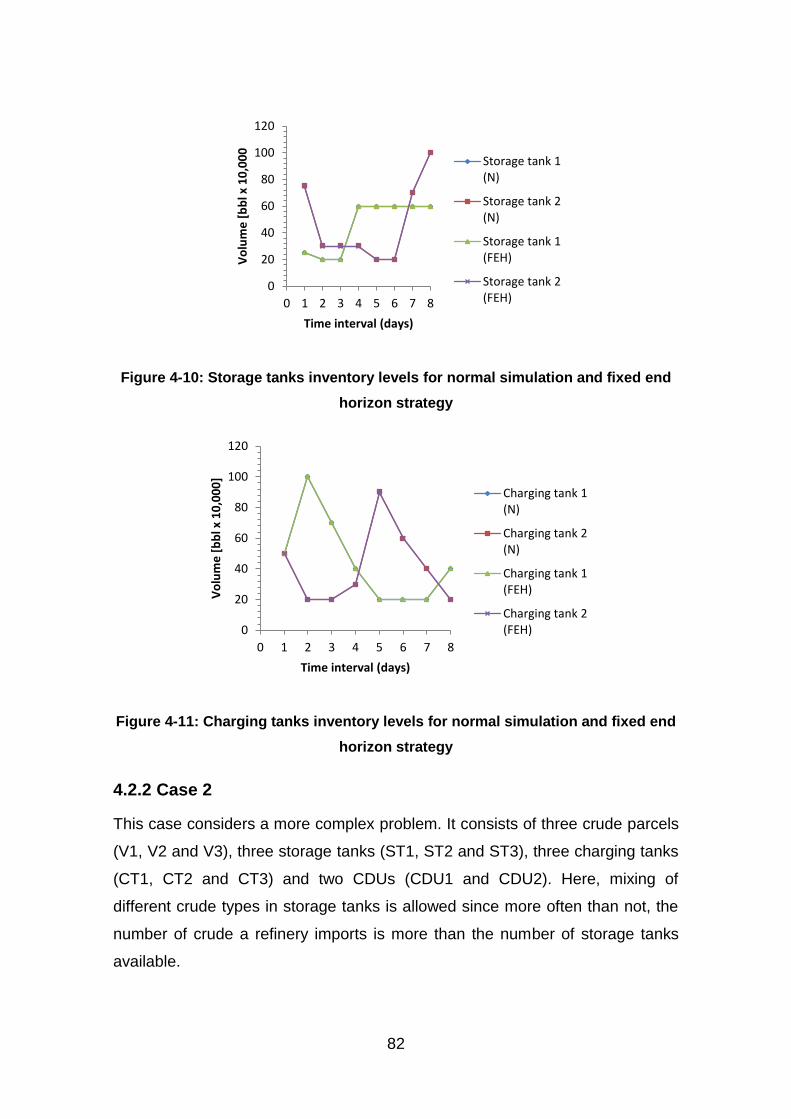
82

Figure 4-10: Storage tanks inventory levels for normal simulation and fixed end

horizon strategy

Figure 4-11: Charging tanks inventory levels for normal simulation and fixed end

horizon strategy

4.2.2 Case 2

This case considers a more complex problem. It consists of three crude parcels

(V1, V2 and V3), three storage tanks (ST1, ST2 and ST3), three charging tanks

(CT1, CT2 and CT3) and two CDUs (CDU1 and CDU2). Here, mixing of

different crude types in storage tanks is allowed since more often than not, the

number of crude a refinery imports is more than the number of storage tanks

available.

0

20

40

60

80

100

120

0 1 2 3 4 5 6 7 8

Vo

lum

e [

bb

l x 1

0,0

00


Storage tank 1(N)

Storage tank 2(N)

Storage tank 1(FEH)

Storage tank 2(FEH)

0

20

40

60

80

100

120

0 1 2 3 4 5 6 7 8

Vo

lum

e [

bb

l x 1

0,0

00

]


Charging tank 1(N)

Charging tank 2(N)

Charging tank 1(FEH)

Charging tank 2(FEH)

83

Using this case study, the two receding horizon strategies discussed earlier are

compared. Data for this case study are obtained from the preceding chapter

with slight modification and presented in Table 4-2.

The optimal CDU charging schedule from the charging tanks is presented in

Figure 4-12. The inventory levels in storage and charging tanks presented in

Figures 4-13 and 4-14 indicate that fixed end strategy approximates the nominal

schedule more closely.

Table 4-2: System information for Case 2


Crude vessels

Arrival time Volume of crude Key component

V1 1st day 500,000 bbl 0.01

V2 5th day 500,000 bbl 0.085

V3 9th day 500,000 bbl 0.06

Storage tanks

Capacities Initial volume(bbl)

Key component Initial(min, max) Min. Max.

ST1 200,000bbl 1,000,000bbl 200,000 0.02(0.01-0.03)

ST2 200,000bbl 1,000,000bbl 200,000 0.05(0.04-0.06)

ST3 200,000bbl 1,000,000bbl 200,000 0.08(0.07-0.09)

Charging tanks

Capacities Initial volume(bbl)

Key component Initial(min, max) Min. Max.

CT1 200,000bbl 1,000,000bbl 300,000 bbl 0.02(0.025-0.035)

CT2 200,000bbl 1,000,000bbl 300,000 bbl 0.05(0.045-0.065)

CT3 200,000bbl 1,000,000bbl 300,000 bbl 0.08(0.075-0.085)



Storage tank inventory unit cost [$/(day x bbl)]

0.004

Charging tank inventory unit cost [$/(day x bbl)]

0.008

Unit changeover cost for charged oil switch in CDU[$]

50,000

Penalty for switching storage tanks when vessel is unloading

8,000

Demand of crude mix from charging tanks to CDU

Blend 1 500,000 bbl

Blend 2 500,000 bbl

Blend 3 500,000 bbl


Vessel to storage tank 0 250,000

Storage tank to charging tank 0 250,000

Charging tank to CDU 200,000 300,000

84

Figure 4-12: CDU charging schedule

Figure 4-13: Storage tanks inventory levels for nominal simulation, fixed end and

moving end horizon strategies

The volume profile of both storage and charging tanks are exactly the same

using traditional approach and with fixed end horizon strategy, hence the two

overlapped in the above figures.

From simulations carried out the fixed end strategy generate feasible and

optimal schedules in all the time steps. But this is not the case for moving end

0

10

20

30

40

50

60

70

80

90

1 2 3 4 5 6 7 8 9 10 11 12

Vo

lum

e [

bb

l x 1

,00

0


Crude mix 1 Crude mix 2 Crude mix 3

20

25

30

35

40

45

50

55

60

0 1 2 3 4 5 6 7 8 9 10 11 12

Vo

lum

e [

bb

l x 1

0,0

00


ST1 (N) ST2(N) ST3(N) ST1(FE) ST2(FE)

ST3(FE) ST1(ME) ST2(ME) ST3(ME)

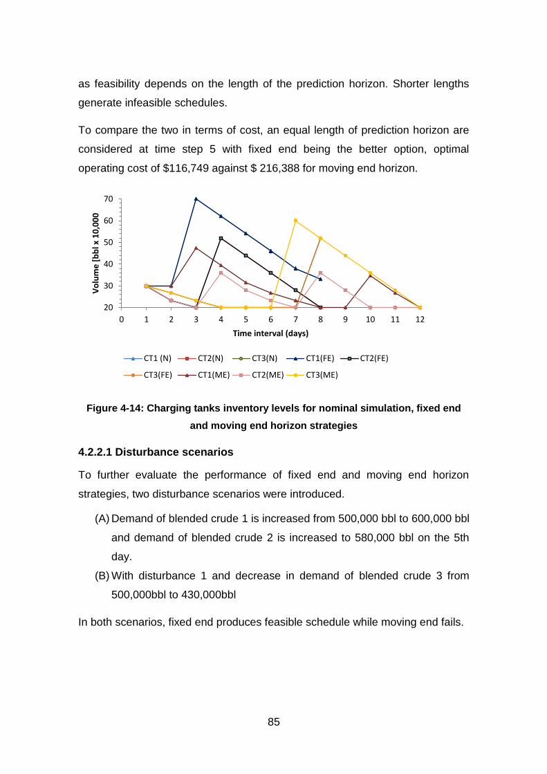
85

as feasibility depends on the length of the prediction horizon. Shorter lengths

generate infeasible schedules.

To compare the two in terms of cost, an equal length of prediction horizon are

considered at time step 5 with fixed end being the better option, optimal

operating cost of $116,749 against $ 216,388 for moving end horizon.

Figure 4-14: Charging tanks inventory levels for nominal simulation, fixed end

and moving end horizon strategies

4.2.2.1 Disturbance scenarios

To further evaluate the performance of fixed end and moving end horizon

strategies, two disturbance scenarios were introduced.

(A) Demand of blended crude 1 is increased from 500,000 bbl to 600,000 bbl

and demand of blended crude 2 is increased to 580,000 bbl on the 5th

day.

(B) With disturbance 1 and decrease in demand of blended crude 3 from

500,000bbl to 430,000bbl

In both scenarios, fixed end produces feasible schedule while moving end fails.

20

30

40

50

60

70

0 1 2 3 4 5 6 7 8 9 10 11 12

Vo

lum

e [

bb

l x 1

0,0

00


CT1 (N) CT2(N) CT3(N) CT1(FE) CT2(FE)

CT3(FE) CT1(ME) CT2(ME) CT3(ME)

86

4.3 Summary of Findings in this Chapter

This chapter presents receding horizon control strategies to deal with

uncertainty in crude oil scheduling problem.

Two of such strategies (fixed-end and moving-end) are introduced as

solution alternatives to handle demand uncertainty.

Results obtained demonstrate that fixed end receding horizon strategy is

a suitable alternative to solve refinery crude oil scheduling problem.

Fixed end receding horizon strategy guarantees feasibility and optimality

under disturbance scenarios.

Fixed end receding horizon outperformed moving end horizon strategy in

terms of performance as schedules are feasible in all the time steps.

Fixed end horizon strategy approximates nominal schedule more closely

and using equal prediction horizon length, it offers lower operational cost

compared to moving end horizon ($116,749 against $ 216,388 at time

step 5).

It has also been shown in this study that crude oil scheduling problem

can be formulated as an optimal control problem.

87

5 SCHEDULING REFINERY PRODUCTION WITH

PRODUCT BLENDING

The downstream of the crude oil unloading and crude distillation unit (CDU)

charging subsystem modelled in Chapter 3 is the refinery production area. This

area formed the main refinery complex where cut fractions are produced from

CDU as refinery intermediate products. Some of these intermediate products

like fuel gas are readily available for sale to customers. The bulk of the

intermediate products are sent to blending units for further processing to meet

certain quality requirements set by customers and environmental laws.

Scheduling of operational tasks is of paramount importance towards maximizing

the overall refinery production income. In refinery production scheduling, certain

features are considered in modelling CDU along with other processing units.

These include the problem formulation as linear or nonlinear; time

representation as discrete or continuous; and whether solution is obtained using

simple, sequential or integrated approach.

Even though mixed integer linear programming (MILP) formulations are used in

refinery modelling such procedure is not sufficient due to the fact that most

processes are nonlinear in nature. Failure to account for nonlinearity will result

in generating unreliable schedules. Issues like this have been spotted in

Chapter 3 where avoiding bilinear terms to maintain model linearity presents

inconsistencies in sulphur concentration for blended crudes. In addition to being

nonlinear, refinery scheduling problems involve discrete and continuous

decisions, hence formulated as mixed integer nonlinear programming (MINLP).

Models presented in Pinto et al. (2000; Méndez et al. (2006); Li et al. (2010);

and Cuiwen et al. (2013) are all MINLPs. The main difference in these refinery

production models lie in the time formulation adopted or developed (discrete or

continuous), problem size and complexity (large-scale or small-scale), and the

solution strategy devised to ensure feasibility and optimality.

Discrete time formulation requires that the length of the scheduling horizon be

divided into a number of time intervals of equal or varying duration. In this

formulation, the beginning and ending of all activities or events are forced to

88

coincide with the boundaries of the time intervals. Binary variables are used to

model the occurrence or non-occurrence of events at these time interval

boundaries. In some way, discrete time formulation simplifies the model but

introduces more binary variables making larger problems intractable or difficult

to solve. The refinery scheduler has to decide on the length of the time interval

to use based on the nature of the problem at hand. Larger time intervals

oversimplify the problem giving inaccurate results. The use of smaller time

intervals gives a more reasonable solution but requires higher computational

efforts as seen in a small scale scheduling problem of crude oil unloading and

CDU charging in Chapter 3.

Unlike the discrete time formulation, the continuous time representation allows

events to occur at any time within the time interval boundaries. The idea is to

split the time horizon into several variable time slots so that events are allowed

to occur at the boundaries of the time intervals. Such formulations introduce

flexibility and possibly eliminate unnecessary event time interval assignments,

thus resulting in problem much smaller in size compared with its equivalent

discrete time representation and hence require less computational efforts

(Floudas and Lin, 2004). Despite these benefits however, variable event timing

makes continuous time models difficult to handle as inventory and material

balance have to be checked at each time slot to ensure solution feasibility

(Méndez et al., 2006). Considering the advantages and limitations in the use of

the aforementioned time representations, the choice between the two is still an

open debate.

Discrete time representation

Continuous time representation

Figure 5-1: Discrete and Continuous time representations (Floudas and Lin, 2004)

89

Recognizing the fact that model development in refinery scheduling is mostly

tied to the solution procedure adopted or developed, a number of concepts are

usually employed; a simple approach that decompose a large problem into

smaller size subproblems and treat the subproblems separately; a sequential

approach that allows exchange of information between subproblems and

integrate the two; and a more rigorous procedure that solves two subproblems

simultaneously. To perform operations in the most efficient way, simultaneous

optimization of production with intermediate product blending is necessary. The

purpose is to effectively schedule the operation based on economic driving

forces while satisfying physical constraints.

5.1 Model Formulation and Problem Definition

In this chapter, a novel MINLP scheduling model for production area with

blending unit is developed to optimize the allocation of materials, distribution of

resources, assignments of tasks and processing times of different crude slates

in a petroleum refinery. The model considers crude oil characteristics with

pseudo-components. In addition to flowrates, crude compositions are also

considered. The CDU model is based on swing cut approach and the objective

of the optimization model is to maximize profit while generating feasible

schedules within time horizon. The scheduling horizon is discretized into a

number of time periods of variable length.


The following technical details are assumed to be available to the refinery

scheduler:

1. A scheduling horizon [0, H].

2. Crude oil assays, compositions and limits on their flow rates.

3. Stream connections.

4. Costs of raw materials: crude oil feeds and butane additives.

5. Unit capacities of CDU and other downstream units along with their

operating costs.

90

6. Yield coefficients of all streams generated from the main refinery

production units with the exception of CDU in which yield is predicted

using swing-cut model approach.

7. Bounds on the intermediate streams properties.

8. B blenders with specification on the component streams to be received at

any given time period.

9. P products with specification on blender processing each of these

products. Lower limits on the blend times and production rates have to

be specified as well. Each blender is assigned to feed a specific product

tank and receives input from specific components streams.

10. Specification limits on the products property indices and revenue realised

from the products sales.

11. Q Product tanks with specification on blenders each storage tank should

receive from. Limits on volume of product in each storage tank at any

given time including time zero and demand for various products are

specified.

12. Product tanks inventory costs.

13. S sales, their constituent products, amounts, and delivery time windows.

With these technical details, the problem here is to find feasible set of

operations that maximize the overall refinery profit by determining the following

decision variables:

1. The type and amount of crude oil processed over time.

2. I components flowrates and their quality indices.

3. Flow profiles of feeds into blending units.

4. Production volume of each blender over time, and the blending duration.

5. The inventory profiles of product tanks.

6. The amount of products available for sale during the scheduling horizon.

5.2 Mathematical Model Development

The motivation here is to come up with a refinery scheduling model that

captures all the necessary interactions between production units and blending

subsystem while solving the two simultaneously.

91

The aforementioned objectives cannot be achieved without some assumptions

and consideration for certain operating rules. They are:

5.2.1 Operating Rules

1. CDU and other upstream units are in continuous operation during the

scheduling horizon.

2. Blenders operate in a semi-continuous mode. When running, blender is

connected to product storage tank and no sales of product at that period

of time. When idle, blender is connected to a dummy storage tank and

product stored in real tank will be available for sale.

3. A blender cannot process more than one product at any time.

4. A blender cannot feed more than one product tank at any time.

5. Products from different blenders can be processed at same time. Such

decision is vital to avoid using tanks unnecessarily.

6. A blender cannot be fed while discharging products.

7. While feeding a blender, a product cannot be discharged at same time.

5.2.2 Model Assumptions

1. The flow of components streams is such that it meets minimum amount

required for blending operation for the whole time periods.

2. Perfect mixing assumption for all blenders.

3. No changeover operations for blenders since specific component

streams are assigned to each blender.

4. No changeover for product storage tanks since each tank is allocated to

a specific product.

5. Each product is processed within the scheduling horizon.

6. All sales involve only one product at a time and multiple products sales

can be decomposed into several single-product sales.

5.2.3 CDU Modelling with Crude Oil Characterization

Considering that crude oil is a complex mixture of components, a good

understanding of its compositional information and thermo-physical properties is

essential. It has been found from a significant number of research studies that

92

obtaining detailed information about the all components is impractical. However,

the crude oil feedstock can be decomposed into hypothetical components called

pseudo-components that can be used in petroleum refinery studies. Unlike the

existing methodologies that use fixed yield approach, refinery scheduling model

developed in this chapter uses pseudo-components and light end hydrocarbon

components to characterize the crude oil and then blended with any swing-cuts

to form the CDU fractions. The pseudo-components were generated using

Aspen plus simulator. The pseudo-components are distributed to the

corresponding cut fractions based on the cuts initial boiling point (IBP) and end

boiling point (EBP).

5.2.3.1 Mass balance for cut fractions

The model starts with mass balance of each cut fraction from a specific crude

oil 𝑐𝑟 at time period 𝑡. The left hand side of Equation 5-1 represents the cut flow

inside the CDU 𝐹𝐶𝑐𝑟,𝑡,𝑓𝑐 which is the sum of the products of crude oil volumetric

flowrate 𝐹𝐵𝑐𝑟,𝑡 and volume fraction of the crude oil components from initial

micro-cuts to final micro-cut 𝑥𝐹𝐵,𝑐𝑟,𝑡. The distribution of the initial micro-cuts 𝑚𝑐

to the corresponding final cut 𝑓𝑐 is based on the boiling range of the target cut

fraction 𝑓𝑟. Equation 5-1 does not include swing cut 𝑠𝑤.

𝐹𝐶𝑐𝑟,𝑡,𝑓𝑐 = ∑𝐹𝐵𝑐𝑟,𝑡𝑥𝐹𝐵,𝑐𝑟,𝑡

𝑓𝑐

𝑚𝑐

∀ 𝑐𝑟,𝑚𝑐, 𝑡, 𝑓𝑐 ≠ 𝑠𝑤

(5-1)

When final micro-cut is a swing cut (𝐹𝐶𝑐𝑟,𝑡,𝑓𝑐=𝑠𝑤), it splits into light 𝑙 and heavy ℎ

streams defined by 𝐹𝑆𝑐𝑟,𝑡,𝑓𝑐=𝑙 and 𝐹𝑆𝑐𝑟,𝑡,𝑓𝑐=ℎ respectively. Thus introducing three

non-negative variables as presented in Equations 5-2 and 5-3. Their values are

optimized to match product quantity and quality specifications.

𝐹𝐶𝑐𝑟,𝑡,𝑓𝑐=𝑠𝑤 = ∑𝐹𝐵𝑐𝑟,𝑡𝑥𝐹𝐵,𝑐𝑟,𝑡

𝑓𝑐

𝑚𝑐

∀ 𝑐𝑟,𝑚𝑐, 𝑡, 𝑓𝑐 = 𝑠𝑤

(5-2)

Equation 5-3 gives the size of the swing cut

𝐹𝐶𝑐𝑟,𝑡,𝑓𝑐=𝑠𝑤 = 𝐹𝑆𝑐𝑟,𝑡,𝑓𝑐=𝑙 + 𝐹𝑆𝑐𝑟,𝑡,𝑓𝑐=ℎ ∀ 𝑐𝑟, 𝑡, 𝑓𝑐 = 𝑠𝑤 (5-3)

93

Flow 𝐹𝑅𝑐𝑟,𝑡,𝑓𝑟 of each cut fraction 𝑓𝑟 can then be computed as the sum of final

micro-cut and its corresponding light 𝑙 and heavy swings ℎ as follows:

𝐹𝑅𝑐𝑟,𝑡,𝑓𝑟 ≤ 𝐹𝐶𝑐𝑟,𝑡,𝑓𝑐 + 𝐹𝑆𝑐𝑟,𝑡,𝑓𝑐=𝑙 + 𝐹𝑆𝑐𝑟,𝑡,𝑓𝑐=ℎ ∀ 𝑐𝑟, 𝑡, 𝑓𝑟 (5-4)

Note that each cut fraction has different swing cut components and the first final

micro-cut has no lighter swing component added to form the corresponding cut

fraction. Similarly, the last final micro-cut has no heavy swing component in the

corresponding cut fraction.

The product yields of CDU is related to the amount of crude oil processed at

any given time instance. i.e.

𝐹𝐵𝑐𝑟,𝑡 ≥ ∑𝐹𝑅𝑐𝑟,𝑡,𝑓𝑟

𝑓𝑟

∀ 𝑐𝑟, 𝑡 (5-5)

5.2.3.2 Mass balance for crude oil

The amount of crude oil to be supplied must satisfy its minimum 𝐹𝐵𝑐𝑟,𝑡,𝑚𝑖𝑛 and

maximum 𝐹𝐵𝑐𝑟,𝑡,𝑚𝑎𝑥 processing requirements. This however, depends also on

the crude oil processing time 𝜑𝑐𝑟,𝑡 and its composition 𝜔𝑐𝑟,𝑡. These are

represented by the following constraints:

𝐹𝐵𝑐𝑟,𝑡 ≥ 𝐹𝐵𝑐𝑟,𝑡,𝑚𝑖𝑛𝜑𝑐𝑟,𝑡 𝜔𝑐𝑟,𝑡 ∀ 𝑐𝑟, 𝑡 (5-6)

𝐹𝐵𝑐𝑟,𝑡 ≤ 𝐹𝐵𝑐𝑟,𝑡,𝑚𝑎𝑥𝜑𝑐𝑟,𝑡 𝜔𝑐𝑟,𝑡 ∀ 𝑐𝑟, 𝑡 (5-7)

While 𝐹𝐵𝑐𝑟,𝑡,𝑚𝑖𝑛 and 𝐹𝐵𝑐𝑟,𝑡,𝑚𝑎𝑥 are in bbl per day, the crude oil processing time

𝜑𝑐𝑟,𝑡 is a fraction of a day. Processing time of crude oil depends on the binary

variable 𝑋𝐶𝑐𝑟,𝑡 which decides whether crude 𝑐𝑟 is processed at time period 𝑡

and the length of the production period 𝐿𝑇𝑡.

𝜑𝑐𝑟,𝑡 = 𝐿𝑇𝑡 𝑋𝐶𝑐𝑟,𝑡 ∀ 𝑐𝑟, 𝑡 (5-8)

The sum of the production period lengths over all time periods gives the length

of the scheduling horizon 𝐻.

94

𝐻 = ∑𝐿𝑇𝑡

𝑡

(5-9)

5.2.4 Downstream Units

The yield, capacity, and quality constraints of other units in the refinery are

formulated in accordance with the stream connections in refinery plants:

The yield of any intermediate product 𝐹𝑠′,𝑢,𝑐𝑟,𝑡, which is the output stream 𝑠′

from unit 𝑢 is obtained by multiplying the yield coefficient 𝜂𝑠′,𝑢,𝑐𝑟,𝑡 with input

(feed) stream 𝑠 to that particular unit (𝐹𝑠,𝑢,𝑐𝑟,𝑡).

𝐹𝑠′,𝑢,𝑐𝑟,𝑡 = 𝜂𝑠′,𝑢,𝑐𝑟,𝑡𝐹𝑠,𝑢,𝑐𝑟,𝑡 ∀ 𝑢, 𝑐𝑟, 𝑡 (5-10)

A stream feeding a unit must satisfy the unit capacity 𝑐𝑎𝑝𝑢 requirement

∑𝐹𝑠′,𝑢,𝑐𝑟,𝑡

𝑠′

≤ 𝑐𝑎𝑝𝑢 ∀ 𝑢, 𝑐𝑟, 𝑡 (5-11)

Streams are connected from one unit to another by means of splitters and

mixers.

For splitters the following constraint holds:

𝐹𝑠,𝑠𝑝𝑙𝑖𝑡,𝑐𝑟,𝑡 = ∑𝐹𝑠′,𝑠𝑝𝑙𝑖𝑡,𝑐𝑟,𝑡

𝑠′

∀ 𝑠𝑝𝑙𝑖𝑡, 𝑐𝑟, 𝑡 (5-12)

Similarly, for mixers the constraint is represented as

∑𝐹𝑠′,𝑚𝑖𝑥,𝑐𝑟,𝑡

𝑠′

= 𝐹𝑠,𝑚𝑖𝑥,𝑐𝑟,𝑡 ∀ 𝑚𝑖𝑥, 𝑐𝑟, 𝑡 (5-13)

A special mixer is the blending unit (blender) that process component streams

from splitters into blends of different quality attributes 𝑘 as specified by

customers. Output streams from blenders 𝐹𝑝,𝑐𝑟,𝑡 are the refinery main products

available for sale.


𝑠′,𝑢

= 𝐹𝑝,𝑐𝑟,𝑡 ∀ 𝑝, 𝑐𝑟, 𝑡 (5-14)

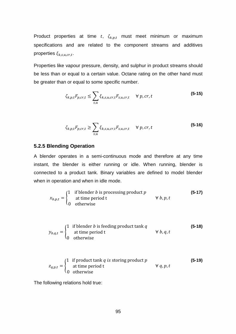
95

Product properties at time 𝑡, 𝜁𝑘,𝑝,𝑡 must meet minimum or maximum

specifications and are related to the component streams and additives

properties 𝜉𝑘,𝑠,𝑢,𝑐𝑟,𝑡.

Properties like vapour pressure, density, and sulphur in product streams should

be less than or equal to a certain value. Octane rating on the other hand must

be greater than or equal to some specific number.

𝜁𝑘,𝑝,𝑡𝐹𝑝,𝑐𝑟,𝑡 ≤ ∑𝜉𝑘,𝑠,𝑢,𝑐𝑟,𝑡𝐹𝑠,𝑢,𝑐𝑟,𝑡

𝑠,𝑢

∀ 𝑝, 𝑐𝑟, 𝑡 (5-15)

𝜁𝑘,𝑝,𝑡𝐹𝑝,𝑐𝑟,𝑡 ≥ ∑𝜉𝑘,𝑠,𝑢,𝑐𝑟,𝑡𝐹𝑠,𝑢,𝑐𝑟,𝑡

𝑠,𝑢

∀ 𝑝, 𝑐𝑟, 𝑡 (5-16)

5.2.5 Blending Operation

A blender operates in a semi-continuous mode and therefore at any time

instant, the blender is either running or idle. When running, blender is

connected to a product tank. Binary variables are defined to model blender

when in operation and when in idle mode.

𝑥𝑏,𝑝,𝑡 = {1 if blender 𝑏 is processing product 𝑝

at time period t 0 otherwise

∀ 𝑏, 𝑝, 𝑡 (5-17)

𝑦𝑏,𝑞,𝑡 = {1 if blender 𝑏 is feeding product tank 𝑞


∀ 𝑏, 𝑞, 𝑡 (5-18)

𝑧𝑞,𝑝,𝑡 = {1 if product tank 𝑞 𝑖𝑠 storing product 𝑝


∀ 𝑞, 𝑝, 𝑡 (5-19)

The following relations hold true:

96

At any time period, if blender 𝑏 feeds tank 𝑞 and that tank stores product 𝑝 then

𝑏 processes 𝑝 at that particular time period. i.e.

𝑥𝑏,𝑝,𝑡 ≥ 𝑧𝑞,𝑝,𝑡 + 𝑦𝑏,𝑞,𝑡 − 1 ∀ 𝑏, 𝑝, 𝑞, 𝑡 (5-20)

If 𝑏 processes 𝑝 and feeds 𝑞 at time period 𝑡, then 𝑞 holds 𝑝 at that particular

time period.

𝑧𝑞,𝑝,𝑡 ≥ 𝑥𝑏,𝑝,𝑡 + 𝑦𝑏,𝑞,𝑡 − 1 ∀ 𝑏, 𝑝, 𝑞, 𝑡 (5-21)

Each blender 𝑏 cannot feed more than one product tank 𝑞 at time period 𝑡. i.e.

∑𝑦𝑏,𝑞,𝑡

𝑞

≤ 1 ∀ 𝑏, 𝑡 (5-22)

Blender cannot simultaneously receive component streams for processing while

feeding storage tank 𝑞. A binary variable 𝑐𝑠𝑠,𝑢,𝑐𝑟,𝑡 is defined to denote that

blender 𝑏 is receiving component streams 𝑠 of crude 𝑐𝑟 from refinery production

unit 𝑢 at time period 𝑡.

𝑐𝑠𝑠,𝑢,𝑐𝑟,𝑡 = {1 if blender b is receiving from component

streams at time period t 0 otherwise

∀ 𝑏, 𝑐𝑟, 𝑡 (5-23)

The following constraint ensures that blender is either receiving component

streams or feeding product tank.

𝑐𝑠𝑠,𝑢,𝑐𝑟,𝑡 + 𝑦𝑏,𝑞,𝑡 ≤ 1 ∀ 𝑏, 𝑐𝑟, 𝑞, 𝑡 (5-24)

Due to semi-continuous nature of its operation, not all the component streams

are processed at the same time in the blender. Component streams that cannot

be processed at a particular time period are temporarily stored to be used at a

later time. Therefore each component stream splits into two non-negative

variables. The amount processed by the blender at any time period is the

fraction of the component streams received at that particular time. Equation 5-

14 can then be transformed to:

97


𝑠′,𝑢

= 𝐹𝑏𝑙𝑒𝑛𝑑,𝑐𝑟,𝑡𝑐𝑠𝑠,𝑢,𝑐𝑟,𝑡 + 𝐹𝑠𝑡𝑜𝑟𝑒𝑑,𝑐𝑟,𝑡 ∀ 𝑏, 𝑐𝑟, 𝑡 (5-25)

The actual amount produced during blending operation 𝐹𝑃𝑝,𝑡 should satisfy the

following constraint

𝐹𝑃𝑝,𝑡𝑥𝑏,𝑝,𝑡 ≤ 𝐹𝑏𝑙𝑒𝑛𝑑,𝑐𝑟,𝑡 ∀ 𝑏, 𝑝, 𝑡 (5-26)

Therefore Equations 5-15 and 5-16 can be re-written as

𝜁𝑘,𝑝,𝑡𝐹𝑃𝑝,𝑡 ≤ ∑𝜉𝑘,𝑠,𝑢,𝑐𝑟,𝑡

𝑠,𝑢

𝐹𝑏𝑙𝑒𝑛𝑑,𝑐𝑟,𝑡 ∀ 𝑘, 𝑝, 𝑡 (5-27)

𝜁𝑘,𝑝,𝑡𝐹𝑃𝑝,𝑡 ≥ ∑𝜉𝑘,𝑠,𝑢,𝑐𝑟,𝑡

𝑠,𝑢

𝐹𝑏𝑙𝑒𝑛𝑑,𝑐𝑟,𝑡 ∀ 𝑘, 𝑝, 𝑡 (5-28)

During operation, a blender runs within its lower 𝑅𝐿𝑝,𝑡,𝑚𝑖𝑛 and upper limits

𝑅𝐿𝑝,𝑡,𝑚𝑎𝑥 and is related to the product processing time 𝜙𝑝,𝑡.

𝜙𝑝,𝑡 ≥ 𝑅𝐿𝑝,𝑡,𝑚𝑖𝑛 (5-29)

𝜙𝑝,𝑡 ≤ 𝑅𝐿𝑝,𝑡,𝑚𝑎𝑥 (5-30)

The volume 𝑉𝑃𝑝,𝑡 produced from each blender depends on the amount

processed by the blender (in bbl per day) and the product processing time (in

hours). Thus,

𝑉𝑃𝑝,𝑡 = 𝐹𝑃𝑝,𝑡𝜙𝑝,𝑡 𝑥𝑏,𝑝,𝑡 (5-31)

The volume produced must be within its production limit and should not be more

the capacity of the blender 𝑐𝑎𝑝𝑏𝑙𝑒𝑛𝑑𝑒𝑟.

𝑉𝑃𝑝,𝑡 ≥ 𝑉𝑃𝑝,𝑡,𝑚𝑖𝑛 (5-32)

98

𝑉𝑃𝑝,𝑡 ≤ 𝑉𝑃𝑝,𝑡,𝑚𝑎𝑥 (5-33)

𝑉𝑃𝑝,𝑡 ≤ 𝑐𝑎𝑝𝑏𝑙𝑒𝑛𝑑𝑒𝑟 (5-34)

5.2.6 Product Storage and Inventory

From mass balance, a material inventory of each product in storage tank

𝐼𝑁𝑃𝑇𝑝,𝑡 can be accounted for. This is calculated as the sum of the initial

inventory in the tank at the beginning of each time period and the actual amount

produced at that period less the actual amount ordered/sold to customers at the

same period.

𝐼𝑁𝑃𝑇𝑝,𝑡+1 = 𝐼𝑁𝑃𝑇𝑝,𝑡 + 𝑉𝑃𝑝,𝑡 − 𝑉𝑃𝑆𝑝,𝑡 (5-35)

𝑉𝑃𝑆𝑝,𝑡 is the actual amount of each product available for sale to customers at

time period 𝑡. This amount must meet the demand 𝐷𝑀𝑝,𝑡 of customers

throughout the scheduling horizon.

𝑉𝑃𝑆𝑝,𝑡 ≥ 𝐷𝑀𝑝,𝑡 (5-36)

The inventory must always be within products’ lower and upper limits and must

not exceed the tank capacity 𝑉𝑃𝑇𝑝.

𝐼𝑁𝑃𝑇𝑝,𝑡 ≥ 𝐼𝑁𝑃𝑇𝑝,𝑡,𝑚𝑖𝑛 (5-37)

𝐼𝑁𝑃𝑇𝑝,𝑡 ≤ 𝐼𝑁𝑃𝑇𝑝,𝑡,𝑚𝑎𝑥 (5-38)

𝐼𝑁𝑃𝑇𝑝,𝑡 ≤ 𝑉𝑃𝑇𝑝𝑧𝑞,𝑝,𝑡 (5-39)

As noted in Chapter 3, it is an operational policy to keep minimum safety stock

above tanks bottom levels in order to safeguard floating device. To prevent

99

tanks from running out of stock at the end of the scheduling horizon, periodic

constraint on the inventory is imposed. i.e.

𝐼𝑁𝑃𝑇𝑝,𝑡+1 ≤ 𝐼𝑁𝑃𝑇𝑝,1 (5-40)

This ensures that low inventory at the end of the scheduling horizon is avoided.

Rebennack et al. (2011) recommends that only one of the storage tanks safety

stock values is fixed while leaving the values for other tanks as variables to be

determined by model solution. This is to avoid being trapped in the infeasibility

region.

5.2.7 Objective Function

The objective function is computed as the overall refinery profit 𝑃𝑅 which is the

revenue generated from selling the products minus all the costs associated with

raw material, unit operation, inventory, purchased intermediate (additive), and

penalties.

𝑃𝑅 = ∑∑𝑝𝑓𝑝 ∗ 𝑉𝑃𝑆𝑝,𝑡 −

𝑝𝑡

∑∑𝑐𝑡𝑐𝑟 ∗ 𝐹𝐵𝑐𝑟,𝑡 ∗ 𝜑𝑐𝑟,𝑡

𝑐𝑟𝑡

− ∑∑𝑔𝑢 ∗ 𝐹𝑠,𝑢,𝑐𝑟,𝑡 ∗ 𝜑𝑐𝑟,𝑡 −

𝑢𝑡

∑∑𝑝𝑠𝑡𝑝 ∗ 𝐼𝑁𝑃𝑇𝑝,𝑡

𝑝𝑡

−∑𝑢𝑖 ∗ 𝐵𝑈𝑇𝑡

𝑡

− ∑𝑝𝑒𝑛𝑎𝑙𝑡𝑖𝑒𝑠

𝑡

(5-41)

The revenue is computed as product of price of product per bbl 𝑝𝑓𝑝 and the total

amount sold to customers 𝑉𝑃𝑆𝑝,𝑡. Raw material cost is obtained by multiplying

the cost per bbl 𝑐𝑡𝑐𝑟 with the amount of crude oil processed 𝐹𝐵𝑐𝑟,𝑡 and the

processing time 𝜑𝑐𝑟,𝑡. Similarly, unit operation cost is the product of cost per bbl

𝑔𝑢 processed in each unit, amount processed in each unit 𝐹𝑠,𝑢,𝑐𝑟,𝑡 and the

processing time 𝜑𝑐𝑟,𝑡. Inventory cost is computed by multiplying inventory cost

per bbl stored 𝑝𝑠𝑡𝑝 with the amount stored 𝐼𝑁𝑃𝑇𝑝,𝑡. Purchased intermediate

(butane) cost is obtained in a similar way, multiplying butane cost per bbl 𝑢𝑖 and

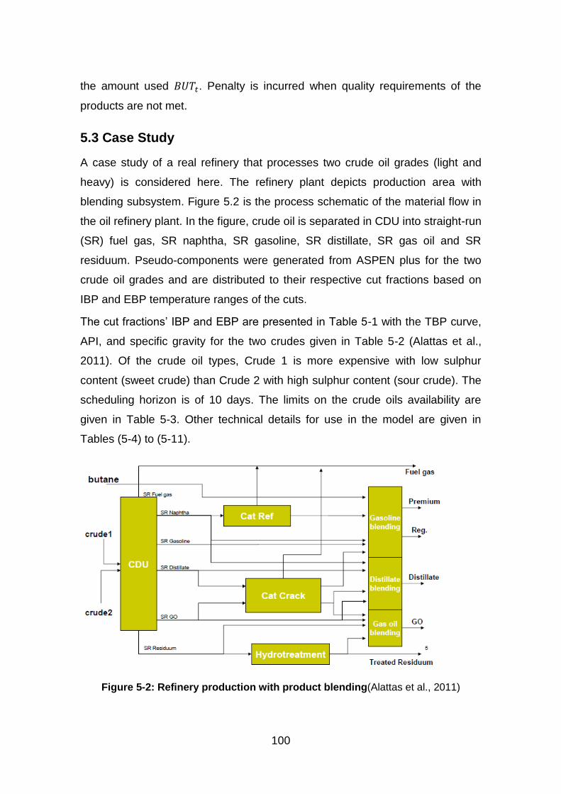
100

the amount used 𝐵𝑈𝑇𝑡. Penalty is incurred when quality requirements of the

products are not met.

5.3 Case Study

A case study of a real refinery that processes two crude oil grades (light and

heavy) is considered here. The refinery plant depicts production area with

blending subsystem. Figure 5.2 is the process schematic of the material flow in

the oil refinery plant. In the figure, crude oil is separated in CDU into straight-run

(SR) fuel gas, SR naphtha, SR gasoline, SR distillate, SR gas oil and SR

residuum. Pseudo-components were generated from ASPEN plus for the two

crude oil grades and are distributed to their respective cut fractions based on

IBP and EBP temperature ranges of the cuts.

The cut fractions’ IBP and EBP are presented in Table 5-1 with the TBP curve,

API, and specific gravity for the two crudes given in Table 5-2 (Alattas et al.,

2011). Of the crude oil types, Crude 1 is more expensive with low sulphur

content (sweet crude) than Crude 2 with high sulphur content (sour crude). The

scheduling horizon is of 10 days. The limits on the crude oils availability are

given in Table 5-3. Other technical details for use in the model are given in

Tables (5-4) to (5-11).

Figure 5-2: Refinery production with product blending(Alattas et al., 2011)

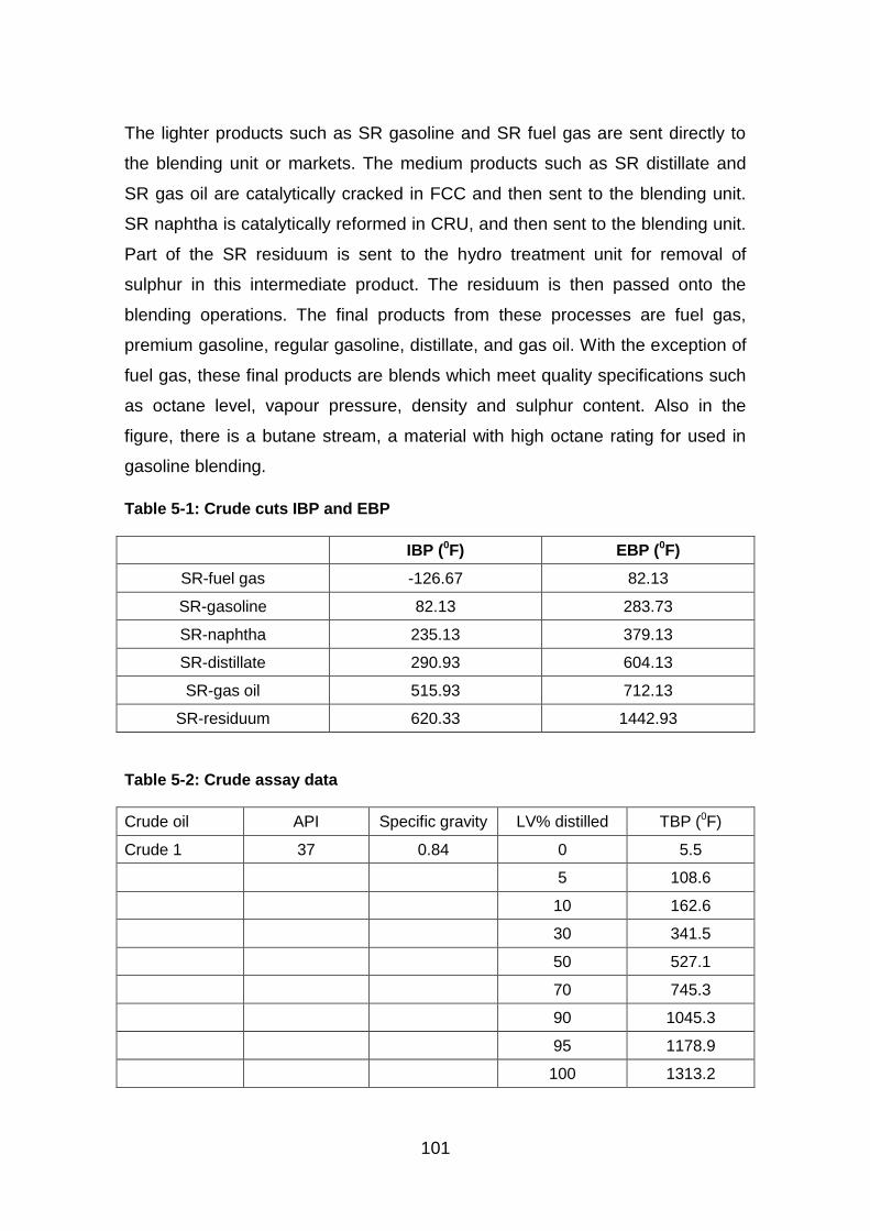
101

The lighter products such as SR gasoline and SR fuel gas are sent directly to

the blending unit or markets. The medium products such as SR distillate and

SR gas oil are catalytically cracked in FCC and then sent to the blending unit.

SR naphtha is catalytically reformed in CRU, and then sent to the blending unit.

Part of the SR residuum is sent to the hydro treatment unit for removal of

sulphur in this intermediate product. The residuum is then passed onto the

blending operations. The final products from these processes are fuel gas,

premium gasoline, regular gasoline, distillate, and gas oil. With the exception of

fuel gas, these final products are blends which meet quality specifications such

as octane level, vapour pressure, density and sulphur content. Also in the

figure, there is a butane stream, a material with high octane rating for used in

gasoline blending.

Table 5-1: Crude cuts IBP and EBP

IBP (0F) EBP (0F)

SR-fuel gas -126.67 82.13

SR-gasoline 82.13 283.73

SR-naphtha 235.13 379.13

SR-distillate 290.93 604.13

SR-gas oil 515.93 712.13

SR-residuum 620.33 1442.93

Table 5-2: Crude assay data

Crude oil API Specific gravity LV% distilled TBP (0F)

Crude 1 37 0.84 0 5.5

5 108.6

10 162.6

30 341.5

50 527.1

70 745.3

90 1045.3

95 1178.9

100 1313.2

102

Crude 2 32.4 0.8631 0 73.7

5 169.8

10 218.9

30 415.9

50 614.2

70 861.5

90 1184.8

95 1339.6

100 1494.2

Table 5-3: Crude oil availability (1000s bbl/day)

Limit/days 1 2 3 4 5 6 7 8 9 10

Minimum 20 20 20 20 20 20 20 20 20 20

Maximum 200 200 200 200 200 200 200 200 200 200

Table 5-4: Refinery raw material/operating costs and product prices

Raw material costs ($/bbl)

Crude 1 75

Crude 2 65

Butane 67.5

Operating costs ($/bbl processed)

Crude distillation 5

Catalytic reformer 7.5

Catalytic cracker 40

Catalytic cracker - Gas oil feed 4

Hydrotreater - Distillate feed 5

Inventory cost 0.00306

Product prices ($/bbl)

Premium gasoline 135

Regular gasoline 121

Distillate 87

Gas oil 76.5

Fuel gas 35

103

Table 5-5: Yield patterns for the downstream process units

Output yields Crude 1 Crude 2

Catalytic reformer

Reformed fuel gas 0.129 0.099

Reformate for gasoline blending 0.807 0.836

Loss 0.064 0.065

1.000 1.000

Catalytic cracker DS GO DS GO

Cracked fuel gas 0.30 0.31 0.36 0.38

Cracked gasoline 0.59 0.59 0.58 0.60

Gas oil (for distillate or gas oil blending) 0.21 0.22 0.15 0.15

1.100 1.12 1.09 1.09

Hydrotreater RS

Desulphurized residuum 0.97

Table 5-6: Capacities of process units (1000 bbl/day)

Crude distillation 100

Catalytic reformer 20

Catalytic cracker 30

Product tank 150

Table 5-7: Blending information from yields

Premium and Regular Gasoline Clear Research Octane Vapour Pressure (mmHg)

SR gasoline (from crude unit) 78.5 18.4

SR naphtha (from crude unit) 65.0 6.54

Reformate (from reformer) 104.0 2.57

Cracked gasoline(from cat cracker)

93.7 6.90

Butane 91.8 199.2

Density (lb/bbl) Sulphur (lb/bbl)

Crude 1 Crude 2 Crude 1 Crude 2

Distillate

SR naphtha (from crude unit) 272.0 272.0 0.283 1.48

SR distillate (from crude unit) 292.0 297.6 0.526 2.83

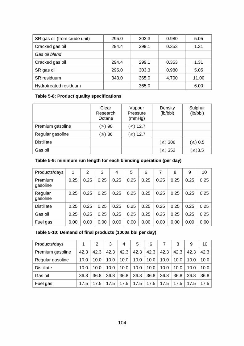
104

SR gas oil (from crude unit) 295.0 303.3 0.980 5.05

Cracked gas oil 294.4 299.1 0.353 1.31

Gas oil blend

Cracked gas oil 294.4 299.1 0.353 1.31

SR gas oil 295.0 303.3 0.980 5.05

SR residuum 343.0 365.0 4.700 11.00

Hydrotreated residuum 365.0 6.00

Table 5-8: Product quality specifications

Clear Research Octane

Vapour Pressure (mmHg)

Density (lb/bbl)

Sulphur (lb/bbl)

Premium gasoline (≥) 90 (≤) 12.7

Regular gasoline (≥) 86 (≤) 12.7

Distillate (≤) 306 (≤) 0.5

Gas oil (≤) 352 (≤)3.5

Table 5-9: minimum run length for each blending operation (per day)

Products/days 1 2 3 4 5 6 7 8 9 10

Premium gasoline

0.25 0.25 0.25 0.25 0.25 0.25 0.25 0.25 0.25 0.25

Regular gasoline

0.25 0.25 0.25 0.25 0.25 0.25 0.25 0.25 0.25 0.25

Distillate 0.25 0.25 0.25 0.25 0.25 0.25 0.25 0.25 0.25 0.25

Gas oil 0.25 0.25 0.25 0.25 0.25 0.25 0.25 0.25 0.25 0.25

Fuel gas 0.00 0.00 0.00 0.00 0.00 0.00 0.00 0.00 0.00 0.00

Table 5-10: Demand of final products (1000s bbl per day)

Products/days 1 2 3 4 5 6 7 8 9 10

Premium gasoline 42.3 42.3 42.3 42.3 42.3 42.3 42.3 42.3 42.3 42.3

Regular gasoline 10.0 10.0 10.0 10.0 10.0 10.0 10.0 10.0 10.0 10.0

Distillate 10.0 10.0 10.0 10.0 10.0 10.0 10.0 10.0 10.0 10.0

Gas oil 36.8 36.8 36.8 36.8 36.8 36.8 36.8 36.8 36.8 36.8

Fuel gas 17.5 17.5 17.5 17.5 17.5 17.5 17.5 17.5 17.5 17.5

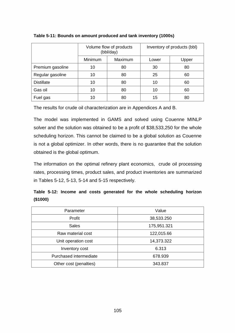
105

Table 5-11: Bounds on amount produced and tank inventory (1000s)

Volume flow of products (bbl/day)

Inventory of products (bbl)

Minimum Maximum Lower Upper

Premium gasoline 10 80 30 80

Regular gasoline 10 80 25 60

Distillate 10 80 10 60

Gas oil 10 80 10 60

Fuel gas 10 80 15 80

The results for crude oil characterization are in Appendices A and B.

The model was implemented in GAMS and solved using Couenne MINLP

solver and the solution was obtained to be a profit of $38,533,250 for the whole

scheduling horizon. This cannot be claimed to be a global solution as Couenne

is not a global optimizer. In other words, there is no guarantee that the solution

obtained is the global optimum.

The information on the optimal refinery plant economics, crude oil processing

rates, processing times, product sales, and product inventories are summarized

in Tables 5-12, 5-13, 5-14 and 5-15 respectively.

Table 5-12: Income and costs generated for the whole scheduling horizon

($1000)

Parameter Value

Profit 38,533.250

Sales 175,951.321

Raw material cost 122,015.66

Unit operation cost 14,373.322


Purchased intermediate 678.939

Other cost (penalties) 343.837

106

Table 5-13: Raw material processing information

period length Crude 1 processed Crude 2 processed

Rate (1000s bbl/day)

Volume (1000s

bbl)

Time (hr) Rate (1000s bbl/day)

Volume (1000s

bbl)

Time (hr)

1 1.336 96.144 128.4484 32.062 72.603 96.99761 32.062

2 0.520 103.984 54.07168 12.478 96.016 49.92832 12.478

3 0.512 102.429 52.44365 12.291 96.245 49.27744 12.291

4 0.504 99.172 49.98269 12.099 100.828 50.81731 12.099

5 0.526 105.149 55.30837 12.618 94.521 49.71805 12.618

6 0.516 103.139 53.21972 12.377 96.861 49.98028 12.377

7 0.875 102.291 89.50463 20.996 96.757 84.66238 20.996

8 1.016 100.041 101.6417 24.380 96.883 98.43313 24.380

9 0.896 179.162 160.5292 21.499 20.838 18.67085 21.499

10 3.300 65.999 217.7967 79.199 65.999 217.7967 79.199

Table 5-14: Product sales

period Product sales (1000s bbl)

Premium gasoline

Regular gasoline

Distillate Gas oil Fuel gas

1 80.319 135 150 150.145 85

2 42.3 10 10 36.8 17.5

3 42.3 10 10.131 36.8 17.5

4 42.3 10 10 43.161 17.5

5 42.3 10 10 50.357 17.5

6 42.3 10 10 61.812 17.5

7 42.3 10 10 69.879 17.5

8 42.3 10 10 76.79 17.5

9 42.3 10 10 61.343 17.5

10 51.303 35 20 89.212 25

107

Table 5-15: Product inventory levels

period Product inventories (1000s bbl)

Premium gasoline

Regular gasoline

Distillate Gas oil Fuel gas

1 150 150 150 150 150

2 80 25 10 26.137 75

3 73.307 25 10 15.632 67.5

4 66.625 25 10 10 60

5 59.807 25 10 10 52.5

6 53.002 25 10 10 45

7 46.509 25 10 10 37.5

8 39.723 25 10 10 30

9 32.609 25 10 10 22.5

10 30 25 10 10 15

5.4 Consideration for Discrete-time with Equal Interval Length

The result presentations and discussions in the preceding section were based

on variable time formulation of the scheduling problem. Results for an

equivalent formulation with equal interval length of time periods are presented

here. An equal interval length of 1 day for the whole scheduling horizon is used.

That is, the 10 day scheduling horizon is discretized into 10 time periods of

equal length. The scheduling problem is then solved again to obtain an optimal

profit of $29,621,550. This is less than the amount $38,533,250 obtained for the

variable length time formulation. The interest here is not to compare the two

solutions directly since the difference in the time formulation means the two

problems are not exactly the same, but to show the benefit of using a better

approach. Optimal refinery plant economics and crude oil processing details for

this uniformly discretized problem are given in Tables 5-16 and 5-17.

108

Table 5-16: Income and costs generated for the whole scheduling horizon

($1000)

Parameter Value

Profit 29,621.550

Sales 172,497.900

Raw material cost 128,489.800

Unit operation cost 13,659.440


Purchased intermediate 720.696

Other cost (penalties) 0

Table 5-17: Raw material processing information

period length Crude 1 processed Crude 2 processed

Rate (1000s bbl/day)

Volume (1000s

bbl)

Time (hr) Rate (1000s bbl/day)

Volume (1000s

bbl)

Time (hr)

1 1 117.224 117.224 12.000 20.000 20.000 12.000

2 1 126.865 126.865 14.759 20.000 20.000 9.241

3 1 168.023 168.023 13.732 20.000 20.000 10.268

4 1 151.038 151.038 12.000 20.000 20.000 12.000

5 1 180.000 180.000 12.000 20.000 20.000 12.000

6 1 119.967 119.967 12.000 80.033 80.033 12.000

7 1 139.872 139.872 12.000 60.128 60.128 12.000

8 1 145.243 145.243 12.000 54.757 54.757 12.000

9 1 143.913 143.913 12.000 56.087 56.087 12.000

10 1 89.254 89.254 12.000 31.839 31.839 12.000

Comparing the two time formulations of the scheduling problem in terms of

costs presented in Table 5-12 (variable timing) and Table 5-16 (uniform

discretization), the later gives larger values in most of the cost components. The

revenue generated with variable timing is higher than the amount obtained

using uniform time discretization. This in turn generates higher profit in favour of

the formulation with varying time periods.

From Table 5-13, it can be observed from the second column that variable time

formulation records the actual duration of each task in a given time period and

109

therefore reflects the actual processing times and hence the amount processed

at each time period. This is not the case for uniform time discretization as

events are forced to take place at the boundary of intervals. Despite the benefits

of variable time formulation as demonstrated in this particular problem, the

approach may be inappropriate in other problems based on the reasons stated

in the introductory part of this chapter.

One interesting thing to observe from processing time columns in Tables 5-13

and 5-17 is that in variable timing the two crudes are processed simultaneously

(in parallel) while in uniform time discretization the crudes are processed

sequentially. This is strange considering that the difference in the two

formulations lie only in the interval timing. This scenario may be an indication

that the solutions obtained are not global.

5.5 Summary of Contributions in this Chapter

In refinery scheduling, model development is in most cases tied to the solution

procedure adopted or developed to solve the model. Most of the existing

methodologies are based on:

1. A simple approach that decompose a large problem into smaller size

subproblems and treat the subproblems separately.

2. A sequential approach that allow exchange of information between

subproblems and integrate the two and,

3. A more rigorous procedure that solves two subproblems simultaneously.

To perform operations in the most efficient way, simultaneous optimization of

production with intermediate product blending is necessary. This is to ensure

reliable schedules are generated while satisfying physical and economic

constraints.

In this chapter, a novel MINLP scheduling model for production area with

blending unit was developed to optimize the allocation of materials,

distribution of resources, assignments of tasks and processing times of

different crude slates in a petroleum refinery.

110

The model considers crude oil characteristics with pseudo-components.

In addition to flowrates, crude oil compositions are also considered

making the model suitable for control studies.

The CDU model is based on swing cut approach and the objective of the

optimization model was to maximize profit while generating feasible

schedules within time horizon.

The scheduling horizon is discretized into a number of time periods of

variable length and then equal length of 1 day was considered thereafter.

A large scale refinery problem was used as a case study to test the

model.

The results obtained from the case study shows that reliable decisions

can be obtained for implementation in real plants.

111

6 REFINERY PRODUCTION WITH UNCERTAINTY IN

CRUDE OIL COMPOSITION

One of the challenges in refinery scheduling is the generation of schedules with

consideration to uncertainty in process parameters. Fluctuation in product

demand, change in crude oil composition, and other uncertainties do manifest

during execution of the schedules. In the presence of these uncertainties, the

schedule generated under deterministic conditions may become infeasible,

suboptimal or difficult to implement. To deal with these uncertainties, a number

of preventive and reactive alternatives are developed in literature. While

preventive scheduling seeks to incorporate uncertainty at the initial stage before

its realization, the reactive scheduling on the other hand takes corrective action

after a disturbance is introduced into the system.

With a robust control action through feedback, uncertainty due to fluctuation in

crude oil composition, change in crude oil flow rate, and change in qualities and

quantities of additives can be addressed. The failure or success in tackling

these issues depends on the efficiency of the algorithm employed. Although the

methodology presented in Chapter 4 can be used effectively to address

uncertainty in the main refinery production area, a more efficient technique that

is able to cancel the effect of disturbances is presented here. The burden

associated with solving optimization problems repeatedly will be avoided. This

viable alternative technique is called self-optimizing control (SOC). It involves

selection of control variables (CVs) so that when the CVs are controlled at their

set points, the overall plant operation is optimal or near optimal even in the

presence of uncertainties. Therefore in this chapter, a data driven SOC strategy

for multi-period scheduling problems will be developed. The performance of the

method will be elucidated using case studies. The next section discussed

general methodology for SOC and will then be followed by data driven SOC for

the problem under consideration.

112

6.1 Self -Optimizing Control Strategy

Most processes in chemical plants including refinery are operated in such a way

that operators set decision variables as set points and with the aid of

proportional integral derivative (PID) controllers, these set points are kept at

their desired values. To satisfy requirements set by environmental laws, operate

within safety limits, survive market competition and to meet tighter quality

specifications of products; plants must operate near optimal. Self-optimizing

control as a strategy helps to achieve the aforementioned objectives by

selecting appropriate control variables (CVs) so that when they are maintained

at their set point values, the overall plant operation is optimal or near optimal

even in the presence of uncertainties (Skogestad, 2000).

When an uncertainty in the form of disturbance is introduced into a chemical

plant, measurements are taken and control actions are implemented to

compensate for the effects of the uncertainty. In the past decades, several

techniques for CV selections have been reported. Most of these techniques

require process models to determine CVs offline and largely depend on the

ability to linearize nonlinear models around their nominal operating points. This

procedure is time-consuming which results in the plant operation being locally

optimal and become impractical where no process model is available (Kariwala,

2007; Alstad and Skogestad, 2007).

Despite the benefits of applying SOC, there are challenges emanating from the

CV selection. The selected CVs must be such that they give acceptable loss

and therefore are able to avoid any need to re-optimize set points when

uncertainties are introduced into the system. Difficulty arising from using model

for SOC has been overcome by incorporating measurements in the optimization

framework. Single measurements or combination of measurements may be

used as CVs. Halvorsen et al. (2003) introduced methods for finding subset or

combination of measurements as controlled variables. Controlling these subset

or combination of measurement at constant set points implies operating the

plant at desired economic condition. Overcoming challenges due to model

linearization requires a global approach.

113

Necessary condition of optimality (NCO) is a viable complementary method that

seeks to overcome the local shortcomings of the existing SOC methodologies

(Jäschke and Skogestad, 2011). François et al. (2005) are of the view that

measurements can be used to enforce NCO in the presence of uncertainty

where the NCO are separated into active constraints and cost sensitivities

(gradients). Owing to the fact that some NCO components are non-measurable

online due to the presence of uncertain parameter in the objective function, Ye

et al. (2012b) proposed that CVs can be selected in such a way that they

approximate unmeasured NCO over the whole uncertain parameter space. The

CVs can then be obtained through regression methods. The CV selection

problem is therefore transformed into a regression problem and does not need

a model to be a priori (Ye et al., 2012a). The difficulty using NCO lies in the

inability to compute the gradient online.

Recently, a methodology was developed by Girei et al. (2014) that computes

CVs as function of measurements from real plant or simulated data using finite

difference approximation. Grema and Cao (2014) extended the methodology to

dynamical systems where the gradient is approximated using Taylor series

expansion. Their approach is not directly applicable for problems involving

mixed integer programming with multiple time periods and therefore a new

methodology has to be developed. This is the motivation behind this chapter.

Therefore in this study, a multi-period data driven approach involving mixed

integer problems to determine CV as a function of measurements is presented.

The methodology is then applied to refinery scheduling problem with

uncertainties in crude oil composition.

6.1.1 Data Driven Self-optimizing Control for Scheduling

Although the methodology is developed to deal with mixed integer problems,

the discussion here will be mainly on scheduling. Generally, scheduling is a

static mixed integer optimization problem with uncertainties in model

parameters represented as disturbances. This can be formulated as

minu 𝐽(u, d) (6-1)

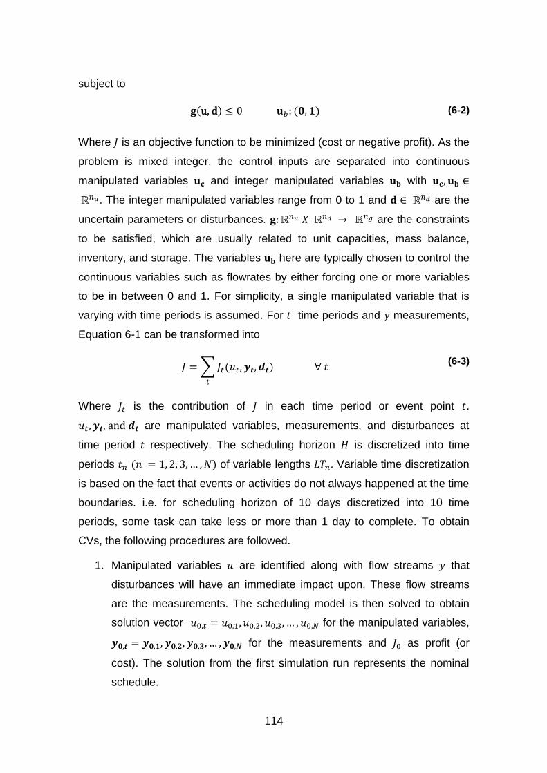
114

subject to

𝐠(u, d) ≤ 0 𝐮𝑏: (𝟎, 𝟏) (6-2)

Where 𝐽 is an objective function to be minimized (cost or negative profit). As the

problem is mixed integer, the control inputs are separated into continuous

manipulated variables 𝐮𝐜 and integer manipulated variables 𝐮𝐛 with 𝐮𝐜, 𝐮𝐛 ∈

ℝ𝑛𝑢. The integer manipulated variables range from 0 to 1 and 𝐝 ∈ ℝ𝑛𝑑 are the

uncertain parameters or disturbances. 𝐠:ℝ𝑛𝑢 𝑋 ℝ𝑛𝑑 → ℝ𝑛𝑔 are the constraints

to be satisfied, which are usually related to unit capacities, mass balance,

inventory, and storage. The variables 𝐮𝐛 here are typically chosen to control the

continuous variables such as flowrates by either forcing one or more variables

to be in between 0 and 1. For simplicity, a single manipulated variable that is

varying with time periods is assumed. For 𝑡 time periods and 𝑦 measurements,

Equation 6-1 can be transformed into

𝐽 = ∑𝐽𝑡(𝑢𝑡, 𝒚𝒕, 𝒅𝒕)

𝑡

∀ 𝑡 (6-3)

Where 𝐽𝑡 is the contribution of 𝐽 in each time period or event point 𝑡.

𝑢𝑡 , 𝒚𝒕, and 𝒅𝒕 are manipulated variables, measurements, and disturbances at

time period 𝑡 respectively. The scheduling horizon 𝐻 is discretized into time

periods 𝑡𝑛 (𝑛 = 1, 2, 3, … ,𝑁) of variable lengths 𝐿𝑇𝑛. Variable time discretization

is based on the fact that events or activities do not always happened at the time

boundaries. i.e. for scheduling horizon of 10 days discretized into 10 time

periods, some task can take less or more than 1 day to complete. To obtain

CVs, the following procedures are followed.

1. Manipulated variables 𝑢 are identified along with flow streams 𝑦 that

disturbances will have an immediate impact upon. These flow streams

are the measurements. The scheduling model is then solved to obtain

solution vector 𝑢0,𝑡 = 𝑢0,1, 𝑢0,2, 𝑢0,3, … , 𝑢0,𝑁 for the manipulated variables,

𝒚𝟎,𝒕 = 𝒚𝟎,𝟏, 𝒚𝟎,𝟐, 𝒚𝟎,𝟑, … , 𝒚𝟎,𝑵 for the measurements and 𝐽0 as profit (or

cost). The solution from the first simulation run represents the nominal

schedule.

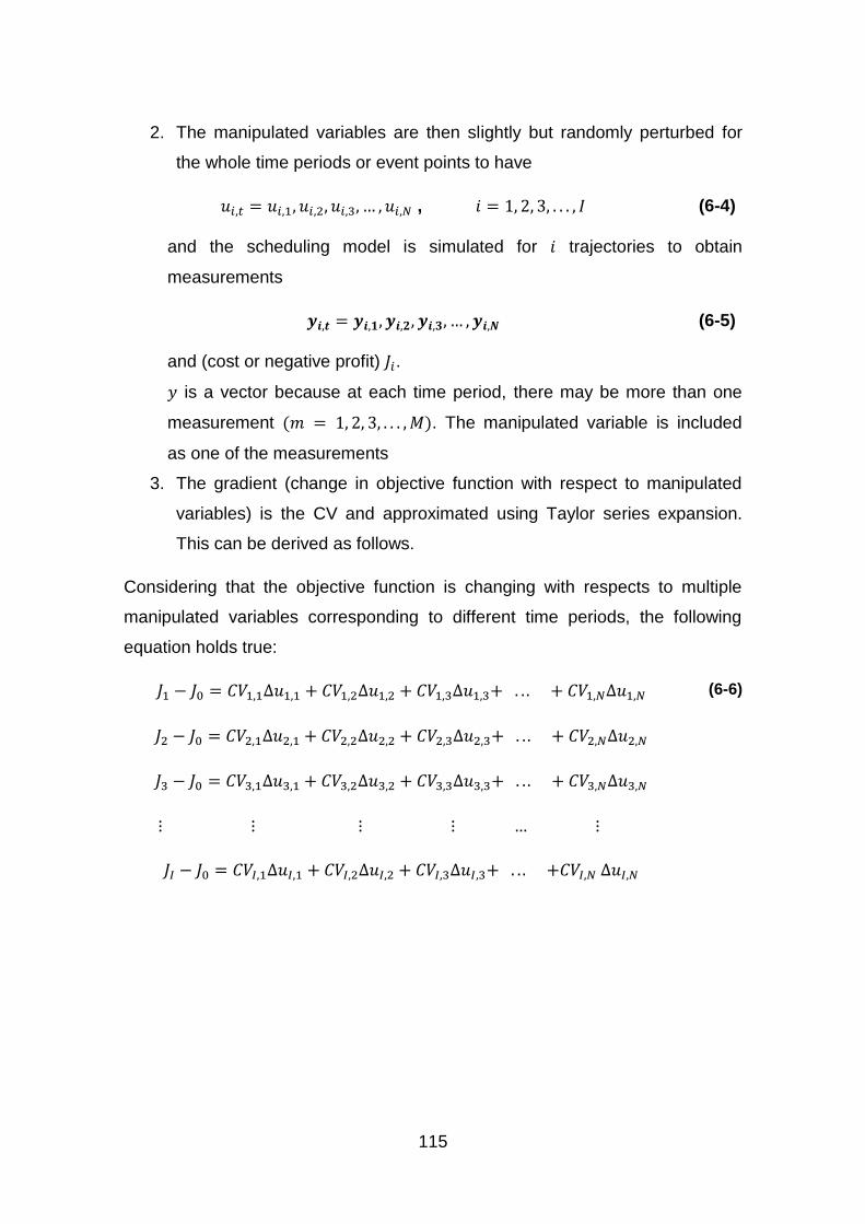
115

2. The manipulated variables are then slightly but randomly perturbed for

the whole time periods or event points to have

𝑢𝑖,𝑡 = 𝑢𝑖,1, 𝑢𝑖,2, 𝑢𝑖,3, … , 𝑢𝑖,𝑁 , 𝑖 = 1, 2, 3, . . . , 𝐼 (6-4)

and the scheduling model is simulated for 𝑖 trajectories to obtain

measurements

𝒚𝒊,𝒕 = 𝒚𝒊,𝟏, 𝒚𝒊,𝟐, 𝒚𝒊,𝟑, … , 𝒚𝒊,𝑵 (6-5)

and (cost or negative profit) 𝐽𝑖.

𝑦 is a vector because at each time period, there may be more than one

measurement (𝑚 = 1, 2, 3, . . . , 𝑀). The manipulated variable is included

as one of the measurements

3. The gradient (change in objective function with respect to manipulated

variables) is the CV and approximated using Taylor series expansion.

This can be derived as follows.

Considering that the objective function is changing with respects to multiple

manipulated variables corresponding to different time periods, the following

equation holds true:

𝐽1 − 𝐽0 = 𝐶𝑉1,1∆𝑢1,1 + 𝐶𝑉1,2∆𝑢1,2 + 𝐶𝑉1,3∆𝑢1,3+ . . . + 𝐶𝑉1,𝑁∆𝑢1,𝑁



⋮ ⋮ ⋮ ⋮ … ⋮

𝐽𝐼 − 𝐽0 = 𝐶𝑉𝐼,1∆𝑢𝐼,1 + 𝐶𝑉𝐼,2∆𝑢𝐼,2 + 𝐶𝑉𝐼,3∆𝑢𝐼,3+ . . . +𝐶𝑉𝐼,𝑁 ∆𝑢𝐼,𝑁

(6-6)

116

Where,

∆𝑢1,1 = (𝑢1 − 𝑢0)1 , ∆𝑢1,2 = (𝑢1 − 𝑢0)2 , . . . , ∆𝑢1,𝑁 = (𝑢1 − 𝑢0)𝑁

∆𝑢2,1 = (𝑢2 − 𝑢0)1 , ∆𝑢2,2 = (𝑢2 − 𝑢0)2 , . . . , ∆𝑢2,𝑁 = (𝑢2 − 𝑢0)𝑁

∆𝑢3,1 = (𝑢3 − 𝑢0)1 , ∆𝑢3,2 = (𝑢3 − 𝑢0)2 , . . . , ∆𝑢3,𝑁 = (𝑢3 − 𝑢0)𝑁

⋮ ⋮ ⋮ ⋮ … ⋮ ⋮

∆𝑢𝐼,1 = (𝑢𝐼 − 𝑢0)1 , ∆𝑢𝐼,2 = (𝑢𝐼 − 𝑢0)2 , . . . , ∆𝑢𝐼,𝑁 = (𝑢𝐼 − 𝑢0)𝑁

(6-7)

The control variables

[ 𝐶𝑉1,1, 𝐶𝑉1,2, 𝐶𝑉1,3, . . . 𝐶𝑉1,𝑁

𝐶𝑉2,1, 𝐶𝑉2,2, 𝐶𝑉2,3, . . . 𝐶𝑉2,𝑁

𝐶𝑉3,1, 𝐶𝑉3,2, 𝐶𝑉3,3, . . . 𝐶𝑉3,𝑁

⋮𝐶𝑉𝐼,1, 𝐶𝑉𝐼,2, 𝐶𝑉𝐼,3, . . . 𝐶𝑉𝐼,𝑁 ]

are non-measurable online and therefore can be replaced with measurement

functions. Thus,

𝐶𝑉1,1 = (𝜃0 + 𝜃1𝑦1,1 + 𝜃2𝑦1,2 + 𝜃3𝑦1,3+. . . +𝜃𝑀𝑦1,𝑀)1

𝐶𝑉1,2 = (𝜃0 + 𝜃1𝑦1,1 + 𝜃2𝑦1,2 + 𝜃3𝑦1,3+. . . +𝜃𝑀𝑦1,𝑀)2

𝐶𝑉2,1 = (𝜃0 + 𝜃1𝑦2,1 + 𝜃2𝑦2,2 + 𝜃3𝑦2,3+. . . +𝜃𝑀𝑦2,𝑀)1

⋮

𝐶𝑉𝐼−1,𝑁 = (𝜃0 + 𝜃1𝑦𝐼−1,1 + 𝜃2𝑦𝐼−1,2 + 𝜃3𝑦𝐼−1,3+. . . +𝜃𝑀𝑦𝐼−1,𝑀)𝑁

𝐶𝑉𝐼,𝑁−1 = (𝜃0 + 𝜃1𝑦𝐼,1 + 𝜃2𝑦𝐼,2 + 𝜃3𝑦𝐼,3+. . . +𝜃𝑀𝑦𝐼,𝑀)𝑁−1

𝐶𝑉𝐼,𝑁 = (𝜃0 + 𝜃1𝑦𝐼,1 + 𝜃2𝑦𝐼,2 + 𝜃3𝑦𝐼,3+. . . +𝜃𝑀𝑦𝐼,𝑀)𝑁

(6-8)

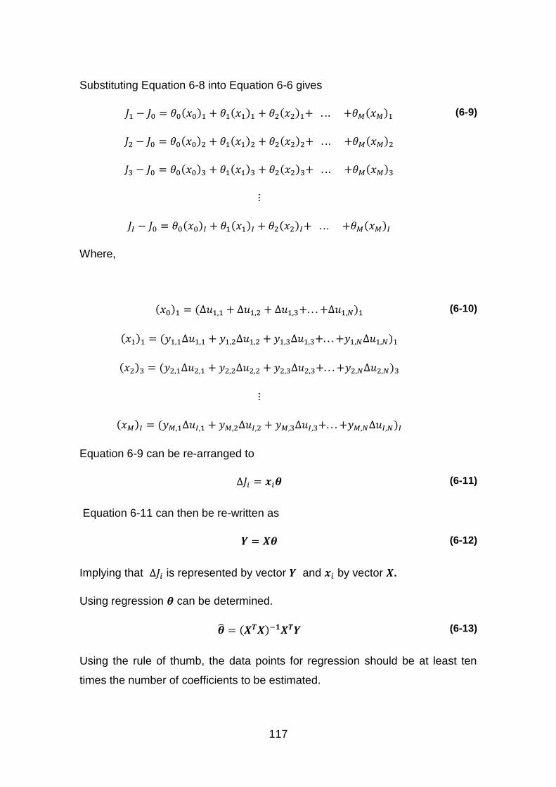
117

Substituting Equation 6-8 into Equation 6-6 gives

𝐽1 − 𝐽0 = 𝜃0(𝑥0)1 + 𝜃1(𝑥1)1 + 𝜃2(𝑥2)1+ . . . +𝜃𝑀(𝑥𝑀)1

𝐽2 − 𝐽0 = 𝜃0(𝑥0)2 + 𝜃1(𝑥1)2 + 𝜃2(𝑥2)2+ . . . +𝜃𝑀(𝑥𝑀)2

𝐽3 − 𝐽0 = 𝜃0(𝑥0)3 + 𝜃1(𝑥1)3 + 𝜃2(𝑥2)3+ . . . +𝜃𝑀(𝑥𝑀)3

⋮

𝐽𝐼 − 𝐽0 = 𝜃0(𝑥0)𝐼 + 𝜃1(𝑥1)𝐼 + 𝜃2(𝑥2)𝐼+ . . . +𝜃𝑀(𝑥𝑀)𝐼

(6-9)

Where,

(𝑥0)1 = (∆𝑢1,1 + ∆𝑢1,2 + ∆𝑢1,3+. . . +∆𝑢1,𝑁)1

(𝑥1)1 = (𝑦1,1∆𝑢1,1 + 𝑦1,2∆𝑢1,2 + 𝑦1,3∆𝑢1,3+. . . +𝑦1,𝑁∆𝑢1,𝑁)1

(𝑥2)3 = (𝑦2,1∆𝑢2,1 + 𝑦2,2∆𝑢2,2 + 𝑦2,3∆𝑢2,3+. . . +𝑦2,𝑁∆𝑢2,𝑁)3

⋮

(𝑥𝑀)𝐼 = (𝑦𝑀,1∆𝑢𝐼,1 + 𝑦𝑀,2∆𝑢𝐼,2 + 𝑦𝑀,3∆𝑢𝐼,3+. . . +𝑦𝑀,𝑁∆𝑢𝐼,𝑁)𝐼

(6-10)

Equation 6-9 can be re-arranged to

∆𝐽𝑖 = 𝒙𝑖𝜽 (6-11)

Equation 6-11 can then be re-written as

𝒀 = 𝑿𝜽 (6-12)

Implying that ∆𝐽𝑖 is represented by vector 𝒀 and 𝒙𝑖 by vector 𝑿.

Using regression 𝜽 can be determined.

�̂� = (𝑿𝑻𝑿)−𝟏𝑿𝑻𝒀 (6-13)

Using the rule of thumb, the data points for regression should be at least ten

times the number of coefficients to be estimated.

118

By analogy, Equation 6-8 can be represented in condensed form as

𝐶𝑉 = 𝜃0 + 𝜃1𝑦1 + 𝜃2𝑦2 + 𝜃3𝑦3+. . . +𝜃𝑀𝑦𝑀 (6-14)

Controlling gradient at zero implies the LHS of Equation 6-14 equal to zero. It is

important to note that 𝑦𝑀,𝑡 is the manipulated variable as mentioned in step 2 of

the solution procedure.

Therefore at each time period, the optimal feedback control input is obtained as:

𝑢𝑓𝑏,𝑡 = −1

𝜃𝑀[𝜃0 + 𝜃1𝑦1 + 𝜃2𝑦2 + 𝜃3𝑦3+. . . +𝜃𝑀−1𝑦𝑀−1]

(6-15)

Some values of the integer manipulated variables may be slightly below 0 or

above 1. In such a case the variables are said to be ‘saturated’ and a constraint

has to be imposed, forcing the saturated variables to be equal to their

corresponding nearest value (0 or 1).

Implementing this feedback strategy in a close loop fashion will incur loss. The

loss can be computed as

𝐿 =𝐽0 − 𝐽(u𝑓𝑏 , d)

𝐽0 × 100

(6-16)

Where 𝐽0 is the true optimal 𝐽, while 𝐽(u𝑓𝑏 , d) is the objective function

corresponding to implementing Equation 6-15 to maintain the CV at zero.

6.2 Case study

The real refinery problem in Chapter 5 is adopted here to show the applicability

of the solution approach developed in this chapter. The same model and same

operational data; the only difference being that the binary variable 𝑋𝐶𝑐𝑟,𝑡 is

allowed to take any value between 0 and 1. The optimal profit 𝐽0 in this case

was obtained as $56,696,407. Allowing 𝑋𝐶𝑐𝑟,𝑡 to include both discrete and

continuous values makes the profit different from the amount $38,533,250

obtained in Chapter 5. The optimal values of the variables 𝑋𝐶𝑐𝑟,𝑡 are used as

parameters in the SOC model. The optimal parameter values of crude 2

(manipulated variables) are then perturbed slightly but randomly around their

119

nominal operating points to form sequence of solutions to be used for

regression analysis. 20x9 (180) data points were generated in accordance with

Equation 6-11 from which 8 regression coefficients are obtained. The

regression coefficients determined are presented in Table 6-1.

Table 6-1: Parameter values from regression

Coefficient Value (x 104)

𝜃0 6.7996

𝜃1 0.1396

𝜃2 0.4154

𝜃3 0.0430

𝜃4 -0.2164

𝜃5 -0.1722

𝜃6 -0.1252

𝜃7 -5.9679

This gives the optimal feedback control law:

𝑢𝑓𝑏,𝑡 = (1/5.9679)[6.7996 + 0.1396𝑦1,𝑡 + 0.4154𝑦2,𝑡 + 0.0430𝑦3,𝑡 − 0.2164𝑦4,𝑡 −

0.1722𝑦5,𝑡 − 0.1252𝑦6,𝑡] (6-17)

The measurements 𝑦1 − 𝑦6 are SR fuel gas, SR gasoline, SR naphtha, SR

distillate, SR gas oil, and SR residuum streams of crude 1 respectively. Cases

with and without uncertainties are considered to illustrate the capability of the

approach presented in this work. Scenarios of different uncertainties were

created and the approach proved to be promising in each situation.

6.2.1 Case 1

This first case assumed no uncertainty is introduced into the system. The

optimal objective value of the base case model with nominal values of the

manipulated variables is compared with the objective value obtained after

feedback implementation with no disturbance. The optimal profit for the base

case model was obtained as $56,696,407. Implementing Equation 6-17 in the

base model results in a profit of $50,523,054. The loss was computed in

120

accordance with Equation 6-16 to obtain a value of 10.888%. Scenarios in the

next case will better illustrate the advantage of SOC.

6.2.2 Case 2

This case considers uncertainties in a number of scenarios to appreciate the

performance of SOC methodology.

6.2.2.1 Scenario A

This scenario consider a change in composition of crude 1 by 5% for the whole

scheduling horizon. The measurements representing cut fractions from crude 1

are taken and the optimal manipulated variable is computed and implemented

in the SOC model to obtain optimal profit 𝐽(u𝑓𝑏 , d) of $53,403,869. Compared

with the optimal value of $56,696,407, a loss of 5.807 % was obtained. The

production levels of the cut fractions using SOC are compared with the actual

amounts produced at the nominal operating conditions. These are shown in

Figures 6-1 to 6-6.

Figure 6-1: Production levels for SR fuel gas at different time periods

0

1

2

3

4

5

6

N1 N2 N3 N4 N5 N6 N7 N8 N9 N10

cu

t fr

ac y

ield

x 1

03 b

bl

Time periods

y1_nom

y1_SOC

121

Figure 6-2: Production levels for SR gasoline at different time periods

Figure 6-3: Production levels for SR naphtha at different time periods

Figure 6-4: Production levels for SR distillate at different time periods

0

5

10

15

20

25

30

N1 N2 N3 N4 N5 N6 N7 N8 N9 N10

cu

t fr

ac y

ield

x 1

03 b

bl

Time periods

y2_nom

y2_SOC

0

5

10

15

20

25

30

35

N1 N2 N3 N4 N5 N6 N7 N8 N9 N10

cut

frac

yie

ld x

10

3 b

bl

Time periods

y3_nom

y3_SOC

0

10

20

30

40

50

60

70

80

N1 N2 N3 N4 N5 N6 N7 N8 N9 N10

cu

t fr

ac y

ield

x 1

03 b

bl

Time periods

y4_nom

y4_SOC

122

Figure 6-5: Production levels for SR gas oil at different time periods

Figure 6-6: Production levels for SR residuum at different time periods

With the exception of SR fuel gas and SR distillate streams from the figures

above, other cut fractions have their production levels approaching minimal

values at the end of the scheduling horizon. Deviations from true optimal values

due to feedback control for the cut fractions is not unconnected with the fact that

refinery production has so many constraints to be satisfied. The amount

produced depends on the CDU processing capabilities. Setting the upper limit

for the crudes to be processed in CDU is an industrial practice that cannot be

ignored. Mandating the plant to operate within this limit will therefore have an

impact on the maximum permissible tuning that will allow the feedback

0

5

10

15

20

25

30

35

N1 N2 N3 N4 N5 N6 N7 N8 N9 N10cu

t fr

ac y

ield

x 1

03 b

bl

Time periods

y5_nom

y5_SOC

0

5

10

15

20

25

30

35

40

45

50

N1 N2 N3 N4 N5 N6 N7 N8 N9 N10

cut

frac

yie

ld x

10

3 b

bl

Time periods

y6_nom

y6_SOC

123

implementation to restore the plant profit. Considering this limitation, the loss of

5.807% obtained is still a reasonable value.

6.2.2.2 Scenario B

In this scenario, a 3% change in composition is considered with the other

information exactly same as in Scenario A. The profit due to feedback

implementation strategy was found to be $54,196,473 against $56,696,407 for

the true optimal value. This translates to 4.409% loss which is better compare to

Scenario A. This improvement is due the magnitude of the disturbance being

smaller in this scenario. Again, based on the reasons mentioned in the

preceding scenario, this loss value of 4.409% is still within the acceptable

range.

6.2.2.3 Scenario C

Here, there is an increase in composition by 9% on the first period then a drop

of 4% is recorded on the fifth period. This scenario is more common in refineries

where fluctuation do occur from one time period to another. The profit recorded

due to SOC is $52,218,634. Comparing with the true optimal value gives a loss

of 7.898%. For the first two time periods, the 𝑢𝑓𝑏 values are -0.0919 and -

0.0444 respectively. These cannot be implemented because 𝒖𝒃 must be

between 0 and 1. Saturation is therefore applied here forcing the two values to

be zero.

The loss value in this scenario is greater than those obtained in Scenarios A

and B due to fact that fluctuation is more intense here with an abrupt change by

9% at the initial stage and a sudden drop by 4% on the fifth period.

In summary, the loss values are greater than 1% in all scenarios because the

refinery plant is a complex with a multiple number of units interconnected and

hence the units cannot be treated independently. Even though decisions from

scheduling are implemented on a day-to-day basis, the schedule generation

does not follow the same pattern. All schedules decisions no matter the length

of the horizon have to be obtained at the same time instance for implementation

at later dates.

124

6.3 Summary of Contributions in this Chapter

Dealing with process uncertainties is one of the main challenges hindering

smooth operations in refinery plants. In such process plants, fluctuation in

product demand, change in crude oil composition, and other parametric

uncertainties in the form of disturbances are very common. In the presence of

those disturbances, schedule generated under deterministic conditions may

become infeasible, suboptimal or difficult to implement. This chapter develops a

reliable methodology under self-optimizing control framework to deal with

uncertainties in mixed integer problems such as those encountered in refinery

scheduling. This contributes to knowledge and below is the highlights of these

contributions.

The methodology addressed problems posed as mixed integer

programming and computes CVs as function of measurements from real

plant or simulated data using Taylor series expansion

The procedure went beyond addressing feasibility issues due to the

influence of uncertain parameters but also ensure optimal or near optimal

operation is maintained. This is first to be reported not only in refinery but

also in the broad area of scheduling as a whole.

The methodology was applied to refinery scheduling problem with

uncertainties in crude oil compositions to come up with a feedback

control law that compensates for the effect of the uncertainties.

Through case studies, the idea presented was able to effectively deal

with the situation at hand with percentage loss within a reasonable

degree.

125

7 CONCLUSIONS AND RECOMMENDATIONS

7.1 Conclusions

The idea to carry out this research was conceived with the aim to develop

robust methodologies and solution procedures to address refinery scheduling

problems under disturbances. The goal was attained through:

1. Developing a mixed integer linear programming formulation for short-

term crude oil unloading, tank inventory management, and crude

distillation unit (CDU) charging schedule as an extension to a previous

work reported by Lee et al. (1996).

2. Investigating the performance of the extended model with case studies.

3. Devising a solution alternative to deal with uncertainty in crude oil

scheduling via model predictive control strategy.

4. Developing a discrete time mixed integer nonlinear programming

(MINLP) formulation for simultaneous optimization of production

scheduling with product blending.

5. Developing a data driven self-optimizing control (SOC) strategy for multi-

period mixed integer problems.

6. Applying the SOC strategy to solve the MINLP model developed in item

(4).

7. Introducing disturbance scenarios (uncertainties in crude oil

compositions) to test the efficacy of the SOC method.

All these were reported in different sections of the thesis.

7.1.1 Modelling Crude Oil Unloading Area

A methodology for short-term crude oil unloading, tank inventory management,

and CDU charging was developed as an extension to Lee et al. (1996) model.

The extended model considers real life issues not captured in the original model

and was built through reformulation in which the problem statement was

modified to account for certain details, and then To investigate the performance

of the model through case studies. The reformulation was based on established

126

operating rules in petroleum refineries, material balances, resource allocations,

sequencing order, product quality, and demand of mixed crude oil.

Scenarios were created to offer recommendations to plant operators on the best

schedule to use. Uncertainties due to disruptive events (CDU shutdown), and

low inventory at the end of scheduling horizon were also considered.

7.1.2 Crude Oil Scheduling under CDU Demand Uncertainty

This section has gone a step beyond forecast on the likelihood of occurrence of

uncertainty by strategizing and devising alternative procedures that generate

more reliable schedules with periodic update to keep track of changes in

process conditions, constraints, or performance criteria. A control technique

usually referred to as model predictive control (MPC) is an alternative that

keeps the decision variables at the required values (set points) while driving the

scheduling process to an economic optimum. A key feature of this control

strategy is that the current implementation of decision variables within the

scheduling horizon can be done more accurately since the process is

periodically updated. One form of MPC is a rolling or receding horizon; a

strategy that allows repeated calculations and predictions updated based on the

current value of decision variable.

In this section of the thesis, scheduling problem of crude oil transfer, blending

and CDU charging has been formulated under the framework of receding

horizon control strategy. The extended model developed in chapter 3 was

adopted. The strategy presented in this study (fixed end) was compared with

the traditional approach and then with another strategy (moving end) using case

studies. Some disturbance scenarios were introduced to evaluate the

performances of fixed end and moving end horizon strategies for

recommendation to refiners and process operators.

Results obtained have shown that fixed end receding horizon strategy can be

relied upon to solve refinery crude oil scheduling problem and was able to

guarantee feasibility and optimality under disturbance scenarios. It

outperformed moving end horizon strategy in terms of performance as

127

schedules are feasible in all time steps. It also approximates nominal schedule

more closely and using equal prediction horizon length, it offers lower

operational cost compared to moving end horizon ($116,749 against $ 216,388

at time step 5).

7.1.3 Scheduling Refinery Production with Product Blending

This section extends the research studies to the main refinery production area

integrated with blending units. The motivation was to come up with a refinery

scheduling model that captures all the necessary interactions between

production units and blending subsystem while solving the two simultaneously.

In refinery scheduling, model development is in most cases tied to the solution

procedure adopted or developed to solve the model. Most of the existing

methodologies are based on:

1. A simple approach that decompose a large problem into smaller size

subproblems and treat the subproblems separately.

2. A sequential approach that allow exchange of information between

subproblems and integrate the two and,

3. A more rigorous procedure that solves two subproblems simultaneously.

To perform operations in the most efficient way, simultaneous optimization of

production with intermediate product blending is necessary. This is to ensure

reliable schedules are generated while satisfying physical and economic

constraints.

This section of the thesis reported a novel MINLP scheduling model for

production area with blending unit to optimize the allocation of materials,

distribution of resources, assignments of tasks and processing times of different

crude slates in a petroleum refinery. The model considers crude oil

characteristics with pseudo-components. In addition to flowrates, crude oil

compositions were also considered making the model suitable for control

studies. Modelling the first unit, CDU was based on swing cut approach and the

objective of the whole refinery model was to maximize profit while generating

feasible schedules within time horizon. A large scale refinery problem was used

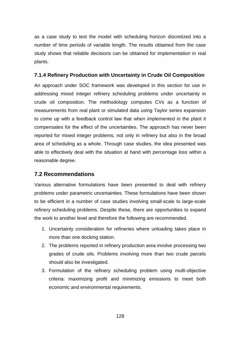
128

as a case study to test the model with scheduling horizon discretized into a

number of time periods of variable length. The results obtained from the case

study shows that reliable decisions can be obtained for implementation in real

plants.

7.1.4 Refinery Production with Uncertainty in Crude Oil Composition

An approach under SOC framework was developed in this section for use in

addressing mixed integer refinery scheduling problems under uncertainty in

crude oil composition. The methodology computes CVs as a function of

measurements from real plant or simulated data using Taylor series expansion

to come up with a feedback control law that when implemented in the plant it

compensates for the effect of the uncertainties. The approach has never been

reported for mixed integer problems, not only in refinery but also in the broad

area of scheduling as a whole. Through case studies, the idea presented was

able to effectively deal with the situation at hand with percentage loss within a

reasonable degree.

7.2 Recommendations

Various alternative formulations have been presented to deal with refinery

problems under parametric uncertainties. These formulations have been shown

to be efficient in a number of case studies involving small-scale to large-scale

refinery scheduling problems. Despite these, there are opportunities to expand

the work to another level and therefore the following are recommended.

1. Uncertainty consideration for refineries where unloading takes place in

more than one docking station.

2. The problems reported in refinery production area involve processing two

grades of crude oils. Problems involving more than two crude parcels

should also be investigated.

3. Formulation of the refinery scheduling problem using multi-objective

criteria: maximizing profit and minimizing emissions to meet both

economic and environmental requirements.

129

4. Data used to compute CVs were generated via model simulation. A real

refinery plant data should give more realistic results.

5. Other uncertain parameters like temperature, pressure and viscosity of

crude feed material should also be considered; separately and then

when all are introduced into the refinery at the same time.

6. Multiparametric programming approach for MINLP problems is still a

challenge that needs to be overcome. This will solve refinery scheduling

problems involving multiple uncertain parameters.

7. Several models for planning and scheduling of refinery systems are

reported separately in literature. The two decision levels are interwoven

with scheduling mainly executing orders set by planning. A model that

integrates planning and scheduling will improve the efficiency and

profitability of a refinery business.

8. An integrated planning and scheduling with consideration to endogenous

and exogenous uncertainties will aid more reliable decisions.

131

REFERENCES

Alattas, A.M., Grossmann, I.E. & Palou-Rivera, I., 2011. Integration of Nonlinear Crude Distillation Unit Models in Refinery Planning Optimization. Industrial & Engineering Chemistry Research, 50(11), pp.6860–6870. Available at: http://pubs.acs.org/doi/abs/10.1021/ie200151e.

Alattas, A. M., Grossman, I. E. & Palou-Rivera, I., 2008. Optimal Model-based Production Planning for Refinery Operations. In AIChE 100-2008 AIChE Annual Meeting, Conference Proceedings.

Alattas, AM, Grossmann, IE & Palou-Rivera, I., 2012. Refinery Production Planning: Multiperiod MINLP with Nonlinear CDU Model. Industrial & Engineering …, 51, pp.12852–12861. Available at: http://pubs.acs.org/doi/abs/10.1021/ie3002638 [Accessed September 21, 2013].

Al-Enezi, G. & Elkamel, A., 2000. Predicting the effect of feedstock on product yields and properties of the FCC process. Petroleum science and technology, 18(2000), pp.407–428. Available at: http://www.tandfonline.com/doi/abs/10.1080/10916460008949853 [Accessed September 5, 2013].

Al-Enezi, G., Fawzi, N. & Elkamel, A., 1999. Development of regression models to control product yields and properties of the fluid catalytic cracking process. Petroleum Science and Technology, 17(5-6), pp.535–552. Available at: http://www.tandfonline.com/doi/abs/10.1080/10916469908949733 [Accessed September 5, 2013].

Al-Qahtani, K. & Elkamel, a., 2010. Robust planning of multisite refinery networks: Optimization under uncertainty. Computers & Chemical Engineering, 34(6), pp.985–995. Available at: http://linkinghub.elsevier.com/retrieve/pii/S009813541000075X [Accessed August 24, 2013].

Alstad, V. & Skogestad, S., 2007. Null space method for selecting optimal measurement combinations as controlled variables. Industrial and Engineering Chemistry Research, 46(3), pp.846–853.

Anon, 2011. Refining flow scheme [Homepage of Honey well company][online]. Available at: http://www.uop.com/refining-flowscheme-2/ [Accessed August 5, 2012].

Antos, G.J. and Aitani, A.M., 2004. Catalytic naphtha reforming 2nd ed., USA.

Aronofsky, J S, Dutton, J M, and Tayyabkhan, M.T., 1978. Managerial Planning with Linear Programming, New York: John Wiley and Sons.

132

Basak, K. et al., 2002. On-Line Optimization of a Crude Distillation Unit with Constraints on Product Properties. Industrial & Engineering Chemistry Research, 41(6), pp.1557–1568. Available at: http://pubs.acs.org/doi/abs/10.1021/ie010059u.

Bassett, M.H., Pekny, J.F. & Reklaitis, G. V., 1996. Decomposition techniques for the solution of large-scale scheduling problems. AIChE Journal, 42(12), pp.3373–3387. Available at: http://doi.wiley.com/10.1002/aic.690421209.

Boesen, R., 2010. Investigation and Modelling of Diesel Hydrotreating Reactions. Available at: http://www.w.seeit-alliance.eu/upload/institutter/ere/phd2011/rasmusrisumboesenphd.pdf [Accessed September 5, 2013].

Cao, C., Gu, X. & Xin, Z., 2009. Chance constrained programming models for refinery short-term crude oil scheduling problem. Applied Mathematical Modelling, 33(3), pp.1696–1707. Available at: http://linkinghub.elsevier.com/retrieve/pii/S0307904X08000772 [Accessed August 25, 2013].

Clay, R.L. & Grossmann, I.E., 1997. A disaggregation algorithm for the optimization of stochastic planning models. Computers & Chemical Engineering, 21(7), pp.751–774. Available at: http://linkinghub.elsevier.com/retrieve/pii/S0098135496002864.

Connor, A.J.O., Introduction to MATLAB. In pp. 1–39.

Cuiwen, C., Xingsheng, G. & Zhong, X., 2013. A Data-Driven Rolling-Horizon Online Scheduling Model for Diesel Production of a Real-World Refinery. AIChE Journal, 59, pp.1160–1174.

Duran, M. & Grossmann, I., 1986. An outer-approximation algorithm for a class of mixed-integer nonlinear programs. Mathematical Programming, 36(3), pp.307–339.

Edgar, T. F., Himmelblau, D. M. & Lasdon, L.S., 2001. Optimization of chemical processes 2nd ed. T. E. Casson, ed., Newyork: McGraw-Hill Chemical Engineering Series.

Ejikeme-Ugwu, E., 2012. Planning for the integrated refinery subsystems. Cranfield University.

Fagundez, F.D. & Faco, J.L.D., 2007. Applying Optimal Control to Jetty Scheduling Problems. MISTA, pp.167–174.

Ferris, M.C., Jain, R. & Dirkse, S., 2011. GDXMRW : Interfacing GAMS and MATLAB. , 53706(February).

133

Floudas, C., 1995. Nonlinear and Mixed-Integer Optimization, New York: Oxford University Press.

Floudas, C. a. & Lin, X., 2004. Continuous-time versus discrete-time approaches for scheduling of chemical processes: a review. Computers & Chemical Engineering, 28(11), pp.2109–2129. Available at: http://linkinghub.elsevier.com/retrieve/pii/S0098135404001401 [Accessed August 10, 2013].

Floudas, C.A. & Lin, X., 2005. Mixed Integer Linear Programming in Process Scheduling: Modeling, Algorithms, and Applications. Annals of Operations Research, 139, pp.131–162.

François, G., Srinivasan, B. & Bonvin, D., 2005. Use of measurements for enforcing the necessary conditions of optimality in the presence of constraints and uncertainty. Journal of Process Control, 15(6), pp.701–712.

Gary, J.H. & Handwerk, G.., 1984. Petroleum Refining Technology and Economics 2nd Editio., Marcel Dekker, Inc.

Geddes, R.L., 1958. A General Index of Fractional Distillation Power for Hydrocarbon Mixtures. AIChE J, 4, pp.389–392.

Girei, A. et al., 2014. Data-driven self-optimizing control. In 24th European Symposium on Computer Aided Process Engineering. pp. 649–654.

Goodwin, G.C. et al., 2006. Receding horizon control applied to optimal mine planning. Automatica, 42(8), pp.1337–1342. Available at: http://linkinghub.elsevier.com/retrieve/pii/S0005109806000720 [Accessed August 19, 2013].

Grema, A.S. & Cao, Y., 2014. Optimal feedback control for reservoir waterflooding. In 20th International Conference on Automation and Computing. pp. 20–25.

Grossmann, IE, Van den Heever, SA & Harjunkoski, I., 2002. Discrete optimization methods and their role in the integration of planning and scheduling. AIChE Symposium …. Available at: http://citeseerx.ist.psu.edu/viewdoc/download?doi=10.1.1.12.1826&rep=rep1&type=pdf [Accessed September 5, 2013].

Guyonnet, P., Grant, F.H. & Bagajewicz, M.J., 2009. Integrated Model for Refinery Planning, Oil Procuring, and Product Distribution. Industrial & Engineering Chemistry Research, 48(1), pp.463–482. Available at: http://pubs.acs.org/doi/abs/10.1021/ie701712z.

134

Halvorsen, I.J. et al., 2003. Optimal Selection of Controlled Variables. Industrial & Engineering Chemistry Research, 42(14), pp.3273–3284. Available at: http://pubs.acs.org/doi/abs/10.1021/ie020833t.

Hamisu, A. A., Kabantiok, S. & Wang, M., 2013. Refinery scheduling of crude oil unloading with tank inventory management. Computers & Chemical Engineering, 55, pp.134–147. Available at: http://linkinghub.elsevier.com/retrieve/pii/S0098135413001105 [Accessed August 24, 2013].

Hamisu, A.A., Kabantiok, S. & Wang, M., 2013. An Improved MILP model for scheduling crude oil unloading, storage and processing. In Computer Aided Chemical Engineering. Elsevier Ltd, pp. 631–636. Available at: DOI: 10.1016/B978-0-444-63234-0.50106-8.

Harjunkoski, I. & Grossmann, I.E., 2001. A decomposition approach for the scheduling of a steel plant production. Computers & Chemical Engineering, 25(11-12), pp.1647–1660. Available at: http://linkinghub.elsevier.com/retrieve/pii/S0098135401007293.

Hopkins, 2012. No Title. Available at: http://www.oilandgasiq.com/glossary/api-gravity/.

Ierapetritou, M.G. & Floudas, C.A., 1998. Effective Continuous-Time Formulation for Short-Term Scheduling. 2. Continuous and Semicontinuous Processes. Industrial & Engineering Chemistry Research, 37, pp.4360–4374.

Ierapetritou, M.G. & Pistikopoulos, E.N., 1996. Batch Plant Design and Operations under Uncertainty. Industrial & Engineering Chemistry Research, 35(3), pp.772–787. Available at: http://pubs.acs.org/doi/abs/10.1021/ie950263f.

Ishuzika, I. T., Ueki, O., Ukamo, U., 2007. Improve refinery margins with integrated planning and scheduling systems,

J. Michalopoulos, S. Papadokonstadakis, G. Arampatzis, A.L., 2001. Modelling of an industrial fluid catalytic cracking unit using neural networks. Chemical Engineering Research and Design, 79(2), pp.137–142. Available at: http://www.sciencedirect.com/science/article/pii/S026387620172028X [Accessed September 6, 2013].

Janak, S.L., Lin, X. & Floudas, C.A., 2007. A new robust optimization approach for scheduling under uncertainty: II. Uncertainty with known probability distribution. Computers & Chemical Engineering, 31, pp.171–195.

Jarullah, A.T., Mujtaba, I.M. & Wood, A.S., 2011. Kinetic parameter estimation and simulation of trickle-bed reactor for hydrodesulfurization of crude oil.

135

Chemical Engineering Science, 66(5), pp.859–871. Available at: http://linkinghub.elsevier.com/retrieve/pii/S0009250910006780 [Accessed August 24, 2013].

Jarullah, A.T., Mujtaba, I.M., and Wood, A.S., 2012. Economic Analysis of an Industrial Refining Unit Involving Hydrotreatment of Whole Crude Oil in Trickle Bed Reactor using gPROMS. In Computer Aided Chemical Engineering. pp. 652–656.

Jäschke, J. & Skogestad, S., 2011. NCO tracking and self-optimizing control in the context of real-time optimization. Journal of Process Control, 21(10), pp.1407–1416.

Jia, Z. & Ierapetritou, M., 2004. Efficient short-term scheduling of refinery operations based on a continuous time formulation. Computers & Chemical Engineering, 28(6-7), pp.1001–1019. Available at: http://linkinghub.elsevier.com/retrieve/pii/S0098135403002394 [Accessed August 21, 2013].

Jia, Z., Ierapetritou, M. & Kelly, J.D., 2003. Refinery Short-Term Scheduling Using Continuous Time Formulation: Crude-Oil Operations. Industrial & Engineering Chemistry Research, 42(13), pp.3085–3097. Available at: http://pubs.acs.org/doi/abs/10.1021/ie020124f.

Joly, M., Moro, L. & Pinto, J., 2002. Planning and scheduling for petroleum refineries using mathematical programming. Brazilian Journal of Chemical …, 19(02), pp.207–228. Available at: http://www.scielo.br/scielo.php?pid=S0104-66322002000200008&script=sci_arttext [Accessed September 6, 2013].

Jones, D.S. and Pujado, P.R., 2006. Handbook of Petroleum Processing, Netherland: Springer.

Kariwala, V., 2007. Optimal measurement combination for local self-optimizing control. Industrial and Engineering Chemistry Research, 46(11), pp.3629–3634.

Kariwala, V., Cao, Y. & Janardhanan, S., 2008. Local self-optimizing control with average loss minimization. Industrial and Engineering Chemistry Research, 47(4), pp.1150–1158.

Karri, B., Srinivasan, R. & Karimi, I. a., 2009. Robustness Measures for Operation Schedules Subject to Disruptions. Industrial & Engineering Chemistry Research, 48(20), pp.9204–9214. Available at: http://pubs.acs.org/doi/abs/10.1021/ie900505a.

Karuppiah, R., Furman, K. & Grossmann, I., 2008. Global optimization for scheduling refinery crude oil operations. Computers & Chemical …, 32,

136

pp.2745–2766. Available at: http://www.sciencedirect.com/science/article/pii/S0098135407002803 [Accessed September 6, 2013].

Kelly, J. & Mann, J., 2003. Crude oil blend scheduling optimization: an application with multimillion dollar benefits. Part 2. Hydrocarbon processing. Available at: http://cat.inist.fr/?aModele=afficheN&cpsidt=14945876 [Accessed August 25, 2013].

Kendrick, D, Meeraus, A, and Suh, J.S., 1981. Oil Refinery Modeling with the GAMS language, Tech. rep., Center of Energy Studies, University of Texas.

Kondili, E., Pantelides, C. & Sargent, R., 1993. A general algorithm for short-term scheduling of batch operations—I. MILP formulation. Computers & Chemical …, 17(2), pp.211–227. Available at: http://www.sciencedirect.com/science/article/pii/009813549380015F [Accessed September 16, 2013].

Kong, M.-T., 2002. Downstream oil products supply chain optimization. Imperial College London.

Kopanos, G.M. & Pistikopoulos, E.N., 2014. Reactive scheduling by a multiparametric programming rolling horizon framework: A case of a network of combined heat and power units. Industrial and Engineering Chemistry Research, 53(11), pp.4366–4386.

Kumar, V. et al., 2001. A crude distillation unit model suitable for online applications. Fuel Processing Technology, 73(1), pp.1–21. Available at: http://linkinghub.elsevier.com/retrieve/pii/S0378382001001953.

Kunii D, L.O., 1991. Fluidisation Engineering 2nd ed., USA: Butterworth–Heinemann.

Lee, H. et al., 1996. Mixed-Integer Linear Programming Model for Refinery Short-Term Scheduling of Crude Oil Unloading with Inventory Management. Industrial & Engineering Chemistry Research, 35(5), pp.1630–1641. Available at: http://pubs.acs.org/doi/abs/10.1021/ie950519h.

Li, J. et al., 2007. Improving the robustness and efficiency of crude scheduling algorithms. AIChE Journal, 53(10). Available at: http://onlinelibrary.wiley.com/doi/10.1002/aic.11280/full [Accessed August 25, 2013].

Li, J., Karimi, I. & Srinivasan, R., 2010. Recipe Determination and Scheduling of Gasoline Blending Operations. AIChE Journal, 56(2), pp.441–465.

137

Li, J., Misener, R. & Floudas, C., 2012a. Continuous‐time modeling and global optimization approach for scheduling of crude oil operations. AIChE Journal, 58(1), pp.205–226. Available at: http://onlinelibrary.wiley.com/doi/10.1002/aic.12623/full [Accessed September 6, 2013].

Li, J., Misener, R. & Floudas, C., 2012b. Scheduling of crude oil operations under demand uncertainty: A robust optimization framework coupled with global optimization. AIChE Journal, 58(8), pp.2373–2396. Available at: http://onlinelibrary.wiley.com/doi/10.1002/aic.12772/full [Accessed September 6, 2013].

Li, W., Hui, C.-W. & Li, A., 2005. Integrating CDU, FCC and product blending models into refinery planning. Computers & Chemical Engineering, 29(9), pp.2010–2028. Available at: http://linkinghub.elsevier.com/retrieve/pii/S0098135405001341 [Accessed August 6, 2013].

Lin, X., Janak, S. & Floudas, C., 2004. A new robust optimization approach for scheduling under uncertainty:: I. Bounded uncertainty. Computers & chemical engineering, 28, pp.1069–1085. Available at: http://linkinghub.elsevier.com/retrieve/pii/S0098135406001591 [Accessed September 13, 2013].

Liu, M. & Sahinidis, N., 1996. Optimization in process planning under uncertainty. Industrial & Engineering Chemistry …, 35(96), pp.4154–4165. Available at: http://pubs.acs.org/doi/abs/10.1021/ie9504516 [Accessed September 6, 2013].

López-García, C. & Roy-Auberger, M., 2003. Analysis and Kinetic Modeling in ULSD Hydrotreating. Prepr. Pap.-Am. Chem. …, 48(2), pp.681–682. Available at: https://web.anl.gov/PCS/acsfuel/preprint archive/Files/48_2_New York_10-03_0666.pdf [Accessed September 5, 2013].

Luo, C. & Rong, G., 2009. A Strategy for the Integration of Production Planning and Scheduling in Refineries under Uncertainty. Chinese Journal of Chemical Engineering, 17(1), pp.113–127. Available at: http://linkinghub.elsevier.com/retrieve/pii/S1004954109600422 [Accessed August 9, 2013].

Majid, M. and Sadat, M.H., 2012. Kinetic Investigation of Catalyst Deactivation in Catalytic Reforming of Naphtha, Chemical Product and Process Modeling. , 7(1).

Méndez, C. a. et al., 2006. A simultaneous optimization approach for off-line blending and scheduling of oil-refinery operations. Computers and Chemical Engineering, 30(4), pp.614–634.

138

Menezes, B.C., Kelly, J.D. & Grossmann, I.E., 2013. Improved swing-cut modeling for planning and scheduling of oil-refinery distillation units. Industrial and Engineering Chemistry Research, 52(51), pp.18324–18333.

Moro, L., Zanin, A. & Pinto, J., 1998. A planning model for refinery diesel production. Computers & Chemical Engineering, 22, pp.1039–1042. Available at: http://www.sciencedirect.com/science/article/pii/S0098135498002099 [Accessed September 6, 2013].

Moro, L.F.L. & Pinto, J.M., 2004. Mixed-Integer Programming Approach for Short-Term Crude Oil Scheduling. Industrial & Engineering Chemistry Research, 43(1), pp.85–94. Available at: http://pubs.acs.org/doi/abs/10.1021/ie030348d.

Mouret, S., Grossmann, I.E. & Pestiaux, P., 2011. A new Lagrangian decomposition approach applied to the integration of refinery planning and crude-oil scheduling. Computers and Chemical Engineering, 35(12), pp.2750–2766. Available at: http://dx.doi.org/10.1016/j.compchemeng.2011.03.026.

Mouret, S., Grossmann, I.E. & Pestiaux, P., 2009. A Novel Priority-Slot Based Continuous-Time Formulation for Crude-Oil Scheduling Problems. Industrial & Engineering Chemistry Research, 48(18), pp.8515–8528. Available at: http://pubs.acs.org/doi/abs/10.1021/ie8019592.

Mula, J. et al., 2006. Models for production planning under uncertainty: A review. International Journal of Production Economics, 103(1), pp.271–285. Available at: http://linkinghub.elsevier.com/retrieve/pii/S0925527306000041 [Accessed August 7, 2013].

Munawar, S. a. & Gudi, R.D., 2005. A Multilevel, Control-Theoretic Framework for Integration of Planning, Scheduling, and Rescheduling. Industrial & Engineering Chemistry Research, 44(11), pp.4001–4021. Available at: http://pubs.acs.org/doi/abs/10.1021/ie040142s.

Neiro, S. & Pinto, J., 2005. Multiperiod optimization for production planning of petroleum refineries. Chem. Eng. Comm., 192(1), pp.62–88. Available at: http://www.tandfonline.com/doi/abs/10.1080/00986440590473155 [Accessed September 6, 2013].

Pan, M., Li, X. & Qian, Y., 2009. New approach for scheduling crude oil operations. Chemical Engineering Science, 64(5), pp.965–983. Available at: http://linkinghub.elsevier.com/retrieve/pii/S0009250908006003 [Accessed August 25, 2013].

Petkov, S.B. & Maranas, C.D., 1997. Multiperiod Planning and Scheduling of Multiproduct Batch Plants under Demand Uncertainty. Industrial &

139

Engineering Chemistry Research, 36(11), pp.4864–4881. Available at: http://pubs.acs.org/doi/abs/10.1021/ie970259z [Accessed September 16, 2013].

Pinto, J.M., Joly, M. & Moro, L.F.L., 2000. Planning and scheduling models for refinery operations. Computers & Chemical Engineering, 24(9-10), pp.2259–2276. Available at: http://linkinghub.elsevier.com/retrieve/pii/S0098135400005718.

Pinto, J.M., Joly, M. & Moro, L.F.L., 2000. Planning and scheduling models for refinery operations. Computers & Chemical Engineering, 24, pp.2259–2276.

Raouf, S., Sukkar, K. & Hamied, R., 2011. Heavy Naphtha Reforming Reactions with Tri-metallic Catalysts, Experimental and Analytical Investigation. Eng. & Tech., 29(10), pp.1917–1935. Available at: http://uotechnology.edu.iq/petrol_tech/papers/dr.khaled and ramzy/Text (5).pdf [Accessed September 6, 2013].

Reddy, P., Karimi, I. & Srinivasan, R., 2003. Short-term scheduling of refinery operations from unloading crudes to distillation. Computer Aided …, pp.304–309. Available at: http://www.sciencedirect.com/science/article/pii/S1570794603805618 [Accessed August 25, 2013].

Rodolfo B. Vadinal, M.R.W.M., 2010. New Method to Simulation of a Vacuum Distillation Unit in the Refining Process of Oil and the Reducing of the Vacuum Residue Generation.

Ronald (Ron) F. and Colwell, P.E., 2010. Oil refinery processes: A brief overview. excellence in applied chemical engineering.

Rosenthal, R.E., 2012. GAMS — A User ’ s Guide. , (January).

Saharidis, G., Minoux, M. & Dallery, Y., 2009. Scheduling of loading and unloading of crude oil in a refinery using event-based discrete time formulation. Computers & Chemical Engineering, 33, pp.1413–1426. Available at: http://www.sciencedirect.com/science/article/pii/S0098135409000659 [Accessed August 25, 2013].

Sahinidis, N. V., 2004. Optimization under uncertainty: state-of-the-art and opportunities. Computers & Chemical Engineering, 28(6-7), pp.971–983. Available at: http://linkinghub.elsevier.com/retrieve/pii/S0098135403002369 [Accessed August 6, 2013].

Sarimveis, H. et al., 2008. Dynamic modeling and control of supply chain systems: A review. Computers & Operations Research, 35(11), pp.3530–

140

3561. Available at: http://linkinghub.elsevier.com/retrieve/pii/S0305054807000366 [Accessed August 10, 2013].

Shah, N. et al., 2009. Centralized–decentralized optimization for refinery scheduling. Computers & Chemical Engineering, 33(12), pp.2091–2105. Available at: http://linkinghub.elsevier.com/retrieve/pii/S009813540900163X [Accessed September 16, 2013].

Shah, N., 1996. Mathematical programming techniques for crude oil scheduling. Computers Chemical Engineering, 20, pp.S1227–S1232.

Skogestad, S., 2000. Plantwide control: The search for the self-optimizing control structure. Journal of Process Control, 10(5), pp.487–507.

Tong, K., Feng, Y. & Rong, G., 2012. Planning under Demand and Yield Uncertainties in an Oil Supply Chain. Industrial & Engineering Chemistry Research, 51(2), pp.814–834. Available at: http://pubs.acs.org/doi/abs/10.1021/ie200194w.

Trierwiler, D., & Tan, R.L., 2001. Advances in crude oil LP modelling. In Hydrocarbon Asia. pp. 52–58.

Verderame, P.M. et al., 2010. Planning and Scheduling under Uncertainty: A Review Across Multiple Sectors. Industrial & Engineering Chemistry Research, 49(9), pp.3993–4017. Available at: http://pubs.acs.org/doi/abs/10.1021/ie902009k.

Wang, J. & Rong, G., 2010. Robust Optimization Model for Crude Oil Scheduling under Uncertainty. Industrial & Engineering Chemistry Research, 49(4), pp.1737–1748. Available at: http://pubs.acs.org/doi/abs/10.1021/ie900358z.

Watkins, R.N., 1979. Petroleum Refinery Distillation 2nd ed., Houston: Gulf Publishing Co.

Wenkai, L. et al., 2002. Scheduling Crude Oil Unloading, Storage, and Processing. Industrial & Engineering Chemistry Research, 41(26), pp.6723–6734. Available at: http://pubs.acs.org/doi/abs/10.1021/ie020130b.

Westerlund, J., Hastbacka, M., Forssell, S. and Westerlund, T., 2007. Mixed-time mixed-integer linear programming scheduling model. Industrial & …, 46, pp.2781–2796. Available at: http://pubs.acs.org/doi/abs/10.1021/ie060991a [Accessed September 16, 2013].

141

Whitcombe, J.M. et al., 2003. Application of sensitivity analysis to oil refinery emissions. Reliability Engineering & System Safety, 79(2), pp.219–224. Available at: http://linkinghub.elsevier.com/retrieve/pii/S0951832002002326.

Whitcombe, J.M. et al., 2006. The use of sensitivity analysis and genetic algorithms for the management of catalyst emissions from oil refineries. Mathematical and Computer Modelling, 44(5-6), pp.430–438. Available at: http://linkinghub.elsevier.com/retrieve/pii/S0895717706000045 [Accessed September 16, 2013].

Ye, L. et al., 2012a. A data-driven approach for selecting controlled variables. Proceedings of 8th Intl. Symposium on …, (2008), pp.904–909. Available at: http://www.nt.ntnu.no/users/skoge/prost/proceedings/adchem-2012/files/0062.pdf [Accessed August 25, 2013].

Ye, L. et al., 2012b. Approximating necessary conditions of optimality as controlled variables. Industrial & Engineering Chemistry …. Available at: http://pubs.acs.org/doi/full/10.1021/ie300654d [Accessed August 25, 2013].

Yee, K.L. & Shah, N., 1998. Improving the efficiency of discrete time scheduling formulation. Computers & Chemical Engineering, 22, pp.S403–S410. Available at: http://linkinghub.elsevier.com/retrieve/pii/S0098135498000817.

Yüzgeç, U., Palazoglu, A. & Romagnoli, J. a., 2010. Refinery scheduling of crude oil unloading, storage and processing using a model predictive control strategy. Computers & Chemical Engineering, 34(10), pp.1671–1686. Available at: http://linkinghub.elsevier.com/retrieve/pii/S0098135410000220 [Accessed August 25, 2013].

Zhang, J., Zhu, X.X. & Towler, G.P., 2001. A Simultaneous Optimization Strategy for Overall Integration in Refinery Planning. Industrial & Engineering Chemistry Research, 40(12), pp.2640–2653. Available at: http://pubs.acs.org/doi/abs/10.1021/ie000367c.

Zhang, N., 2006. Optimisation Is Key to High-performing Refineries. , 7(1983), pp.33–35.

Zhang, N. & Zhu, X., 2000. A novel modelling and decomposition strategy for overall refinery optimisation. Computers & Chemical Engineering, 24, pp.1543–1548. Available at: http://www.sciencedirect.com/science/article/pii/S0098135400005457 [Accessed September 6, 2013].

143

APPENDICES

Appendix A

Table A-1: Initial micro-cuts distribution into their respective cuts for Crude 1

Component Volume fraction of assay

H2O 0.001

C1 0.002

SR-fuel gas C2 0.005

C3 0.005

IC4 0.01 SW1

NC4 0.01

IC5 0.005

SR-gasoline

NC5 0.025

PC139F 0.0239693196

PC162F 0.0251433162

PC189F 0.025690828

PC212F 0.0273153472

PC238F 0.0286375053

PC263F 0.0294267661 SW2

PC287F 0.0295128286

PC312F 0.0288756885 SR-naphtha

PC337F 0.0277672152

PC363F 0.0276849889 SW3

PC387F 0.027788517

PC412F 0.0276623392

SR-distillate PC438F 0.0273168272

PC462F 0.0267776536

PC487F 0.0260826898

144


PC512F 0.0252686212

PC537F 0.0248484816

SW4 PC562F 0.0248378783

PC587F 0.0245594129

PC612F 0.0240364511 SR-gas oil

PC637F 0.0233162189

PC662F 0.0224594729

SW5 PC687F 0.0215234731

PC712F 0.0205555674

PC737F 0.0196598374

SR-residuum

PC763F 0.020217673

PC787F 0.0211685451

PC825F 0.0418487309

PC875F 0.036875742

PC925F 0.0306862509

PC974F 0.0255985838

PC1024F 0.0217873207

PC1074F 0.0192086146

PC1125F 0.0182555212

PC1175F 0.0185063718

PC1250F 0.0372011744

PC1344F 0.00492822657

1

145

Appendix B

Table B-1: Initial micro-cuts distribution into their respective cuts for Crude 2


H2O 0

C1 0.001

SR-fuel gas C2 0.0015

C3 0.009

IC4 0.004 SW1

NC4 0.016

IC5 0.012

SR-gasoline

NC5 0.017

PC189F 0.017688523

PC212F 0.0280123511

PC238F 0.0254032232

PC263F 0.0254280205 SW2

PC287F 0.0254205875

PC312F 0.0254077956 SR-naphtha

PC337F 0.0253895924

PC363F 0.0253660942 SW3

PC387F 0.02533726

PC412F 0.025354157

SR-distillate

PC438F 0.0258397715

PC462F 0.0262087565

PC487F 0.0262517514

PC512F 0.025960761

PC537F 0.0253743275 SW4

PC562F 0.0245530724

146


PC587F 0.0235752844

PC612F 0.0225884769 SR-gas oil

PC637F 0.022163461

PC662F 0.0217942605

SW5 PC687F 0.0213562878

PC712F 0.0208646828

PC737F 0.0203341352

SR-residuum

PC763F 0.0197780962

PC787F 0.0192082949

PC825F 0.0366941323

PC875F 0.0370493138

PC925F 0.040925623

PC974F 0.0381689435

PC1024F 0.0316427922

PC1074F 0.0257917206

PC1125F 0.0214923226

PC1175F 0.0183725942

PC1250F 0.0321279838

PC1344F 0.0320375374

PC1447F 0.0305380121

1

a process flow diagram of an oil refinery plant

Documents