a probability programming language: development and

W&M ScholarWorks W&M ScholarWorks

Dissertations, Theses, and Masters Projects Theses, Dissertations, & Master Projects

1998

A probability programming language: Development and A probability programming language: Development and

applications applications

Andrew Gordon Glen College of William & Mary - Arts & Sciences

Follow this and additional works at: https://scholarworks.wm.edu/etd

Part of the Computer Sciences Commons, and the Statistics and Probability Commons

Recommended Citation Recommended Citation Glen, Andrew Gordon, "A probability programming language: Development and applications" (1998). Dissertations, Theses, and Masters Projects. Paper 1539623920. https://dx.doi.org/doi:10.21220/s2-1tqv-w897

This Dissertation is brought to you for free and open access by the Theses, Dissertations, & Master Projects at W&M ScholarWorks. It has been accepted for inclusion in Dissertations, Theses, and Masters Projects by an authorized administrator of W&M ScholarWorks. For more information, please contact [email protected].

https://scholarworks.wm.edu/

https://scholarworks.wm.edu/etd

https://scholarworks.wm.edu/etds

https://scholarworks.wm.edu/etd?utm_source=scholarworks.wm.edu%2Fetd%2F1539623920&utm_medium=PDF&utm_campaign=PDFCoverPages

http://network.bepress.com/hgg/discipline/142?utm_source=scholarworks.wm.edu%2Fetd%2F1539623920&utm_medium=PDF&utm_campaign=PDFCoverPages

http://network.bepress.com/hgg/discipline/208?utm_source=scholarworks.wm.edu%2Fetd%2F1539623920&utm_medium=PDF&utm_campaign=PDFCoverPages

https://dx.doi.org/doi:10.21220/s2-1tqv-w897

mailto:[email protected]

INFORMATION TO USERS

This manuscript has been reproduced from the microfilm master. UMI

films the text directly from the original or copy submitted. Thus, some

thesis and dissertation copies are in typewriter face, while others may be

from any type of computer printer.

The quality of this reproduction is dependent upon the quality of the

copy submitted. Broken or indistinct print, colored or poor quality

illustrations and photographs, print bleedthrough, substandard margins,

and improper alignment can adversely afreet reproduction.

In the unlikely event that the author did not send UMI a complete

manuscript and there are missing pages, these will be noted. Also, if

unauthorized copyright material had to be removed, a note will indicate

the deletion.

Oversize materials (e.g., maps, drawings, charts) are reproduced by

sectioning the original, beginning at the upper left-hand comer and

continuing from left to right in equal sections with small overlaps. Each

original is also photographed in one exposure and is included in reduced

form at the back of the book.

Photographs included in the original manuscript have been reproduced

xerographically in this copy. Higher quality 6” x 9” black and white

photographic prints are available for any photographs or illustrations

appearing in this copy for an additional charge. Contact UMI directly to

order.

UMIA Bell & Howell Information Company

300 North Zeeb Road, Ann Arbor MI 48106-1346 USA 313/761-4700 800/521-0600

R ep ro d u ced with p erm issio n o f th e copyrigh t ow n er. Further reproduction prohibited w ithout p erm issio n .

Reproduced with permission of the copyright owner. Further reproduction prohibited without permission.Reproduced with permission of the copyright owner. Further reproduction prohibited without permission.

A P ro b a b ility P rogram m in g Language:

D ev e lo p m en t and A p p lica tion s

A Dissertation

Presented to

T h e Faculty of the D epartm ent of A pplied Science

T h e College of W illiam M ary in Virginia

In P artia l Fulfillment

Of the Requirements for the Degree of

Doctor of Philosophy

by

Andrew G. Glen

1998

R ep ro d u ced with p erm issio n o f th e copyrigh t ow n er. Further reproduction prohibited w ithout p erm ission .

UMI Number: 9904264

C o p y r i g h t 19 9 9 b y G le n , A n d re w G o rd o n

All rights reserved.

UMI Microform 9904264 Copyright 1998, by UMI Company. All rights reserved.

This microform edition is protected against unauthorized copying under Title 17, United States Code.

UMI300 North Zeeb Road Ann Arbor, MI 48103


A PPR O V A L SH E ET

This Dissertation is subm itted in partia l fulfillment of

the requirem ents for the Degree of

Doctor of Philosophy

Andrew G. Glen

A PP R O V E D . January 1998

Low 'Mad ILawrence M. Leemis, D issertation Advisor

/LS / A .J S A n / V . . X S . ^

John H. Drew

Sidney H. Lawrence

Rex K. Kincaid

/ \ AA^

Donald R. Barr,O utside Exam iner


C ontents

1 In tro d u c tio n 2

1.1 General ........................................................................................................................ 2

1.2 L itera tu re r e v i e w ...................................................................................................... 6

1.3 O utline of the d i s s e r t a t i o n .................................................................................... 7

1.4 N otation and nom enclature ................................................................................ S

2 Software D evelopm ent 10

2.1 The com mon d a ta s t r u c t u r e ................................................................................ 13

2.2 Comm on continuous, univariate d is t r ib u t io n s ............................................... 16

2.3 T he six representations of d i s t r i b u t io n s .......................................................... IS

2.4 V e r i fy P D F .............................................................................................................. 21

2.5 M e d i a n R V ..................................................................................................................... 24

2.6 DisplayRV ................................................................................................................ 25

2.7 P l o t D i s t .................................................................................................................... 26

2.S Expect a t i o n R V ......................................................................................................... 28

2.9 T r a n s f o r m .............................................................................................................. 29

iii


2.10 O r d e r S t a t ................................................................................................................ 31

2.11 ProductRV and P r o d u c t l l D ............................................................................ 33

2.12 SumRV and S u m l l D .............................................................................................. 36

2.13 MinimumRV................................................................................................................ 3S

2.14 MaximumRV................................................................................................................ 39

2.15 M axim um likelihood e s t i m a t i o n .......................................................................... 41

3 T ransfo rm ations of U n iv aria te R andom V ariables 44

3.1 I n t r o d u c t i o n .................................................................................................................. 44

3.2 T h e o r e m ......................................................................................................................... 47

3.3 I m p l e m e n t a t i o n .......................................................................................................... 50

3.4 Exam ples ..................................................................................................................... 53

3.5 C o n c lu s io n ..................................................................................................................... 59

4 P ro d u c ts o f R andom V ariables 61

4.1 I n t r o d u c t i o n ................................................................................................................. 61

4.2 T h e o r e m ........................................................................................................................ 62

4.3 I m p l e m e n t a t i o n .......................................................................................................... 65

4.4 Exam ples ..................................................................................................................... 68

4.5 C o n c lu s io n ..................................................................................................................... 75

5 C om puting th e C D F of th e K olm ogorov-Sm irnov Test S ta tis tic 76

5.1 I n t r o d u c t i o n ................................................................................................................. 76

5.2 L ite ra tu re r e v i e w ..................................................................................................... 78

iv


•5.3 C om puting the d is tr ibu tion of D n ...................................................................... 79

5.3.1 Phase 1: P a r t i t ion the support of D n — ^ ....................................... S2

5.3.2 Phase 2: Define the A m a t r i c e s ............................................................ S3

5.3.3 Phase 3: Set limits on the app rop ria te i n t e g r a l s ............................. S9

5.3.4 Phase 4: Shift the d i s t r ib u t io n ................................................................ 96

5.4 Critical values and significance l e v e l s .............................................................. 99

5.5 C o n c lu s io n ..................................................................................................................... 100

6 G oodness of F it using O rd e r S ta tis tics 102

6.1 I n t r o d u c t i o n ................................................................................................................. 102

6.2 The V - v e c t o v .............................................................................................................. 104

6.3 Improving com puta tion of V ................................................................................ 106

6.4 Goodness-of-fit t e s t i n g ........................................................................................... 109

6.5 C o n c lu s io n ..................................................................................................................... 113

7 O ther A pplications and E xam ples 115

7.1 I n t r o d u c t i o n ................................................................................................................. 115

7.2 Exactness in lieu of CLT a p p r o x im a t i o n s ...................................................... 116

7.3 A m athem a tica l resource g e n e r a t o r ................................................................. 121

7.4 Probabilis tic model design: reliability block d i a g r a m s ............................. 125

7.5 M odeling with hazard f u n c t i o n s ......................................................................... 127

7.6 O utlie r d e t e c t i o n ...................................................................................................... 132

7.7 M axim um likelihood of order statistics d i s t r i b u t i o n s .................................. 136

v


8 Conclusion and F u rther W ork 140

A T he A rc tangen t Survival D istrib u tio n 143

A .l I n t r o d u c t io n ................................................................................................................. 143

A.2 Development ............................................................................................................. 145

A.3 Probabilistic p r o p e r t i e s ........................................................................................... 14S

A.4 S tatistical in fe re n c e ................................................................................................... 150

A.5 C o n c lu s io n ..................................................................................................................... 15S

B C ontinuous D istribu tions 159

C A lgorithm for 6 x 6 Conversions 161

D A lgorithm s for Various P rocedures 163

D.l A lgorithm for V e r i fy P D F ....................................................................................... 163

D.2 A lgorithm for E x p e c t a t i o n R V ............................................................................ 164

D.3 A lgorithm for O r d e r S t a t ....................................................................................... 165

D.4 A lgorithm for P r o d l l D ........................................................................................... 166

D.5 A lgorithm for S u m R V .............................................................................................. 167

D.6 A lgorithm for S u m llD .............................................................................................. 168

D.T A lgorithm for MinimumRV....................................................................................... 169

D.S A lgorithm for MaximumRV....................................................................................... 170

D.9 Algorithm for MLE..................................................................................................... 171

E A l g o r i t h m for Transform 172

v i


F A lgorithm for ProductRV 174

G A lgorithm for KSRV 180

H Sim ulation C ode for MLEOS A pproxim ations 184

B ibliography 187

Vita 191

v i i


A cknow ledgem ent

I m ust gratefully acknowledge the assistance of m any people who have helped in

very many ways in the production of this dissertation a n d research. Professors Hank

Krieger. M arina K ondratovitch gave help in specific p a r ts of this research. A special

note of personal thanks goes to Professors Donald B arr, J o h n Drew, and especially

Larry Leemis. who were trem endously patient, insightful, and supportive of th e re

search. I th an k for their patience and support my wife, Lisa G len, and my children

Andrea. Rebecca, and Mary. I also thank and praise a lm igh ty G od, for it is only

by His divine will th a t we are privileged to unders tand w hat we have learned in this

process.

vm


»o »

o

List o f Figures

3.1 T he transform ation Y = <7 (A") = X 2 for — 1 < A" < 2 ................................... 54

3.2 T h e transform ation Y = g [ X) = ||A’ — 3| — 1| for 0 < X < 7 .................... 55

3.3 T he transform ation Y = g ( X) has a discontinuity and is variously

I —to—1 and 2 - to - l on different subse ts of the support of A"...................... 57

3.4 T he transform ation Y = <7 (A") = sin2(.A) for 0 < A’ < 2 ~ ........................... 58

4.1 T he support of X and Y w hen ad < be.............................................................. 64

4.2 T h e m apping of Z = X and 1’ = AT" when ad < be..................................... 65

4.3 T he P D F of I ' = A T ' for A" ~ N ( 0 .1) and Y ~ N (0 .1)............................... 72

.1 T h e C D F of the D$ random variab le ................................................................... 98

.2 T h e P D F of the £>6 random variable. Note the d iscontinuity a t y = 1/6. 99

6.1 Transform ations from iid observations A'i , A ^ , . . . ,A 'n to th e sorted

■P-vector elements F(i). P(2), • • • , P(n)...................................................................

6.2 E s tim ated power functions for te s t ing Ho'. X ~ N ( 0 ,1) versus Hi:

X ~ N(0.<72) using K -S , A -D , and two statistics based on th e V-

vector ................................................................................................................................. I l l

ix

7.1 O verlaid plots of f z - { x ) and th e s tan d a rd normal P D F ............................. 120

7.2 Overlaid plots of the s tan d a rd norm al and s tandard ized IG(O.S) d is tr i

bu tio n s .............................................................................................................................. 123

7.3 R B D of a com puter system w ith two processors and th ree m em ory units. 126

7.4 T h e SF of the hypothesized B T -shaped hazard function fit to the sam

ple [1. 11. 14. 16. 17] overlaid on the em pirical S F ........................................ 129

7.5 T h e P D F of the d is tr ibution having periodic hazard function k \ with

param eters a = 1. 6 = 0.5 and c = 10.................................................................. 131

7.6 T h e P D F s of the four order s ta t is t ic s from an exponentia l d is tribution. 13S

A .l Exam ples of the arctangent p robab il i ty density function .......................... 147

A.2 Em pirical, fitted arctangent, an d fitted Weibull survivor functions for

th e ball bearing lifetimes........................................................................................... 153

A.3 T h e arc tangen t d istribution fit to the rat cancer d a t a ............................... 157

x


List o f Tables

5.1 C om pu ta tiona l requirements for com puting the Dn C D F for small n.

5.2 C om pu ta tiona l efficiency associated with using the F and V arrays. .

5.3 CD Fs of D n — ^ for n = 1. 2 , . . . . 6 ......................................................................

6.1 E s tim ated critical values for P, a t various sample sizes and levels of

significance......................................................................................................................

7.1 Fractiles for exact and approxim ated d is tr ibu tions .......................................

7.2 P ( A (6) > 10) for n = 6 for several population d is tr ibu tions ......................

7.3 The M SEs of the MLE and MLEOS and adjusted-for-bias M LE tech

niques of pa ram ete r estim ation ..............................................................................

A.l Kolmogorov-Smirnov Goodness-of-fit S tatis tics for the Ball Bearing

D a ta ...................................................................................................................................

B.l C ontinuous distributions of random variables available in A P P L . . . .

C .l The conversions of continuous random variable d is tr ibu tion forms.

xi


A bstract

A probability p rogram m ing language is developed and presented: app lica tions illustra te its use. Algorithms an d generalized theorem s used in p ro b ab il i ty are encapsulated into a program m ing env ironm en t with the com puter a lg e b ra sy s tem M aple to provide the applied com m unity w ith au to m ated probability capab ili t ies . A lgorithms of procedures are presented and explained , including detailed p re sen ta t io n s on th ree of the most significant procedures. A pplications th a t encom pass a w ide range of applied topics including goodness-of-fit te st ing , probabilistic m odeling, c en tra l l im it theorem augm entation , generation of m a th em a tica l resources, and e s t im a t io n are presented.

xii


A P ro b a b ility P rogram m in g L anguage:

D ev elo p m en t and A p p lica tio n s


C hapter 1

Introduction

1.1 G eneral

Probability theory, as it exists today, is a vast collection of axioms and theorem s tha t,

in essence, provides the scientific com m unity many con tribu tions, including:

• the nam ing and descrip tion of random variables th a t occur frequently in appli

cations.

• the theoretical results associated with these random variables, and,

• the applied results associated w ith these random variables for sta tis tica l appli

cations.

No one volume categorizes its work in exactly these th ree ways, b u t the l i te ra tu re ’s

comprehensive works accom plish these goals. W hether volum inous, such as the work

of Johnson, Kotz. and B alakrishnan (1995), or succinct, such as th a t of Evans, Hast-

2


3

ings, and Peacock (1993). one finds all th ree of these areas presen ted in chap ters that

are organized on th e first contribution above, nam ing and describing th e random vari

ables. Works such as Hogg and Craig (1995), P ort (1994). and David (19S1) organize

their efforts according to the second con tribu tion , covering theo re tica l results that

apply to random variables. Then there are the works such as Law and K elton (1991),

Lehmann (19S6). and D ’Agostino and S tephens (1986) who co n ce n tra te on the sta

tistical applications of random variables, an d ta ilor the ir exp lanations of probability

theory to the portions of the field th a t have application in s ta t is t ic a l analysis.

In all these works, as well as countless o thers , one s tark omission is apparent.

There is no m ention of an ability to a u to m a te th e naming, processing, or application

of random variables. This omission is even more profound when one considers the

tedious na tu re of th e m athem atics involved in th e execution of m any of these results

for all but the sim plest of examples. In practice, th e level of te d iu m makes the

actual execution un tenab le for many random variables. A utom ation of certa in types

of these procedures could eradicate this ted ium . T here is an a b u n d an c e of s tatistical

software packages th a t give the scientific com m unity powerful tools to app ly s tatis tical

procedures. B ut to date , there is no package th a t a t tem p ts to a u to m a te the more

theoretical side of th e probabilist 's work. Even the simplest of tasks, p lo tting a fully

specified probability density function, is not provided in m any s ta t is t ic a l packages.

In order to plot new. ad-hoc densities or C D Fs. one is often required to w rite an

appropria te program.

R ep ro d u ced with p erm issio n o f th e cop yrigh t ow ner. Further reproduction prohibited w ithout p erm issio n .

4

A conceptual p robab il i ty software package is now presen ted th a t begins to fill this

existii g gap. Before ou tl in ing this work's approach, let us p resen t some examples to

il lustrate w hat should be included in such a probability software package.

Consider the following independent ran d o m variables: W ~ gammafA. k), Z ~

N(/x,cr), Y ~ Weibullf A. k). A’ and R ~ arctan(<z>. a ) , and D . T . U . an d V as spec

ified in the questions below. See A ppendix A for more in form ation on the a rc tan

dis tr ibu tion .

• W h a t is the d is tr ibu tion of V’ = W + X + K?

• W h a t is the d is tr ibu tion of T = X • ln (W 2) + eYZ?

• W h a t is the d is tr ib u tio n of a random distance D, which is th e sum of the

p roduc t of random rates Ri. R 2 R n and random tim es T 1 . T 2 Tn. i.e.,

D = Ri • T\ + /?2 • T2 + • • • + R n ■ TvZ-

• W hat is the d is tr ibu tion of the system lifetime U in a re liability block d iagram

containing two parallel blocks of two subsystem s th a t consist of two com ponents

in series, i.e.. U = m ax{m in{V ’. W }, min{V’. Z } } ?

• W h a t is the exact u pper tail probability for the s ta t is t ic 6.124 associated with

th e d is tr ibu tion of th e 4th o rder s ta t is t ic out of a sam ple of 12 iid observations

th a t have the sam e d is tr ibu tion as U?

• How m ight one use th e previous result to improve goodness-of-fit testing?

5

• How could one employ the P D F s of order s tatistics of a popula tion , instead of

the P D F of the popula tion itself, to develop an a l te rna te approach to m axim um

likelihood es tim ation?

• W h a t is the d is tr ibu tion of the m ax im um likelihood es t im a to r of the inverse

Gaussian random variable 's first p a ram ete r /j. when a sam ple size of n is speci

fied?

• Most im portan tly , if one could find these answers, w hat is the ir utility to the

s ta tis tica l and applied science com m unity?

T here is no im plication th a t th e previously cited au thors are remiss in neglect

ing the au tom ation of probability software. In fact it is only with the advent and

m aturing of com puter a lgebra system s, such as Maple and M athem atica , tha t the re

now exists the ability to a u to m a te probabilistic modeling and research. This doc

toral research and d isserta tion will take advantage of this relatively new technology

by developing and presenting a software "engine" th a t con tribu tes to the fields of

probabilistic m odeling and s ta tis tica l applications. This research has concentrated

on procedures in the symbolic language Maple V.

T he specific con tribu tions to the applied probability and s ta t is t ics com m unity of

this research and d isserta tion include the following:

1. D etailed algorithm s th a t com prise the conceptual software.

2. Generalized versions of theorem s th a t comprise the software. [Note th a t while

the theorem s them selves m ay exist in more general forms, the ir general forms

R ep ro d u ced with p erm issio n o f th e copyrigh t ow ner. Further reproduction prohibited w ithout p erm issio n .

6

appear difficult to im plem ent in an au tom ated environm ent.]

3. An a lgori thm th a t produces th e exact C D F of th e Kolmogorov-Smirnov test

s ta tis tic .

4. Detailed explanations and exam ples of the software's capabilities.

5. A pplication examples th a t contribute , on the ir own. to various areas within

probability and statistics.

6. Explorative examples of probabilistic quests th a t appea r to be difficult to carry

out w ithou t autom ation .

7. Extensions of testing s ta tis tica l hypotheses, to include specific contributions in

the areas of outlier detection , goodness-of-fit. and pa ram ete r estimation.

S. D em onstrations in the general area of probabilistic model design, to include

specific contributions in the areas of survival d is tr ibu tions , reliability block di

agrams. exac t solutions to centra l limit theorem (CLT) applications, and es ti

mation.

1.2 L iteratu re rev iew

While the cu rren t l i tera tu re will be reviewed th roughou t the dissertation, there are

a number of works tha t should be mentioned for th e ir general applicability to this

research. T hese include the works of Johnson, Kotz, an d B alakrishnan (1995), Leemis

(1995), Port (19S4). Rohatgi (1976). and others th a t provide the foundation for the


theory behind the algorithm s and im plem entation . T he review of the l i te ra tu re has

discovered no publication on im plem enting probabilis tic procedures in c o m p u te r al

gebra languages, nor on the benefits of such a paradigm . Databases searched include

F irs tSearch , INNOPAC. IN SPEC . D TIC , N T IC . Science C ita tion Index. L ibrary of

Congress. Swem Library at T he College of W illiam k Mary, and the USM A library

at West Point. NY. Search strings included th e following individual sub jec t areas and

pairs of sub jec t areas, where appropria te : d is tr ibu tions , goodness-of-fit. life testing ,

Maple, modeling, order s tatis tics, probability, reliability, and symbolic algebra. W hile

the re are m any listings under these term s and pairings of these term s, no work was

found ab o u t combining probabilistic results w ith com puter a lgebra im plem en ta tion .

T h e negative result of this search indicates th a t the re is a lack of archival m a te r ia l

on the sub jec t .

1.3 O u tlin e o f th e d isser ta tio n

This d isserta tion is presented according to th e following outline. In C h ap te r 2 the

developm ent, abilities, and exam ples of use of the software language are presented.

C h ap te r 3 contains the developm ent of the procedure th a t accom m odates tran sfo rm a

tions of random variables to include a re-s ta ted , general, im plem entable theo rem for

such work. In C hapter 4 a procedure for finding th e d is tr ibu tion of the p ro d u c t of two

independen t continuous random variables is presented. In C h ap te r 5 a p rocedure th a t

re tu rns th e d is tribution of th e K olm ogorov-Sm irnov goodness of fit s ta t is t ic , given a


s

specified sam ple size, is p resented . C hap te r 6 contains an application in w hich a new

goodness-of-fit test p rocedure is presented and tested using the software. C h a p te r 7

is a collection of exam ples of explorations in the fields of probability an d s ta t is t ic s

th a t are now possible due to the softwaxe. Finally, in C h ap te r S. conclusions and

suggestions of fu rther work are given. In the appendices are listed th e a lgo ri thm s for

th e software, as well as docum en ta t ion of the early work in crea ting new probab ilis tic

models.

1.4 N o ta tio n an d n om en clatu re

This section reviews ce r ta in no ta tion and nom enclature used here. Use is m a d e of

th e following acronyms and functional notation for density representations:

• probability density function (P D F ) f x i* ) -

• cum ulative d is tr ibu tion function (CD F) F.y(x) = f x {*) ds,

• surv ivor function (SF) 5.\'(-r) = I — F.v(x).

• haza rd function (H F) h. \{x) =

• cum ulative hazard function (C H F) Hx[ x ) = j l ^ h x i s ) ds, and

• inverse d is tr ibu tion function (ID F) F ^ l (x).

T h ro u g h o u t the d isserta tion , the proposed software is referred to as “a p robab il i ty

p rog ram m ing language" (A P P L ) for brevity. The term s “piecewise” and “seg m en ted ”


9

are used to refer to P D F s (and o ther functions) th a t can be cons truc ted by piecing

together various s ta n d a rd functions, such as polynomials, logarithm s, exponentials,

and trigonom etric functions, e.g., the tr iangu la r( l , 2. 3) d is tr ibu tion which has two

segments or two pieces, each of which are linear functions. T h e com mon abbrev i

ation “N {fj., <r)’’ is used to refer to the normal d istribu tion . N ote th a t the second

param eter is the s ta n d a rd deviation, not the variance. Also, “11(0. 6)” is used to rep

resent the uniform d is tr ibu tion with paxameters a and 6. Subscrip ts in parentheses

represent o rder s ta t is t ic s , e.g. the r th order s ta tis tic associated w ith a random sam ple

A 'i,A '2 X n is d eno ted by A"(r ). The abbreviation “iid” is used to denote inde

penden t and identically d is tr ibu ted random variables. T he te rm s “fully-specified,”

“semi-specified," and “unspecified’’ are used to describe the degree to which p a ram

eters are specified as constan ts or fixed param eters in a d is tr ibu tion . For exam ple,

the exponential! 1) d is tr ibu tion is a fully specified d is tr ibu tion . T h e W eibull(l , k )

and the N(0. a) are bo th semi-specified distributions. T he tr iangu la r(a . b. c) and

exponential!A) d is tr ibu tions are both unspecified. T ypew rite r font is used to rep

resent Maple language s ta tem en ts . For example “> X := U niform RV (0, 1 ) ; " is a

M aple assignment s ta te m e n t . Note th a t the symbol “>” represents the Maple inpu t

p rom pt and is not typed .

R ep ro d u ced w ith p erm iss io n o f th e copyrigh t ow n er. Further reproduction prohibited w ithout p erm issio n .

C hapter 2

Software D evelopm ent

T he notion of probability software is different from the notion of app lied s ta tis tica l

software. Probability theory is rife with theorems and calculations th a t require sym

bolic. algebraic m anipulations. Applied sta tis tica l calculations are usually numeric

m anipula tions of d a ta based on known formulas associated with d is tr ibu tions of com

mon random variables. This section contains a discussion on several a lgorithm s th a t

con tribu te to the development of APPL. Availability of com pu te r a lgebra systems

such as M aple and M athm atica facilitate the development of software th a t will derive

functions, as opposed to com puting numbers.

P robab ility software m ust, a t the most basic level, be a means of producing dis

tr ibu tions of random variables. At the heart of the software m ust reside an “engine”

th a t can com pute new. useful representations of distributions.

T h e derivation of exact d is tr ibu tion functions of complex random variables is often

untenable. In such cases, one had to be content w ith approx im ations and sum m ary

10


11

s ta t is t ic s of the unknown d is tributions, regardless of w hether those app rox im ations

and sum m aries were adequate . For exam ple, one often approxim ates d is tr ibu tions us

ing M onte Carlo simulation or by invoking th e centra l l im it theorem. S ta t is tics such

as th e sam ple mean and variance of the ap p ro x im ated d is tribu tion are then reported .

If w ha t was really needed was a certain percen tile of the approxim ated d is tr ibu tion ,

often tim es the entire sim ulation would need to be remodeled, re-validated, re-verified,

and re-run to obta in the needed inform ation. A result such as a fully-specified P D F

would erad icate the need for such redundan t efforts. O ne also would have a n a ly t

ical results to represent characteristics of ce r ta in com plex random variables whose

fully-specified functions are untenable. For exam ple, renewal theory and com pound

Poisson process theory have results th a t derive the m ean and variance of com plex dis

tr ibu tions . but fall short of ac tually determ in ing the en tire representation of com plex

d is tr ibu tions via a PD F. C D F. or some o th e r form of the distribution. T he proposed

probabilistic software is designed to make a b reak th rough into the area of com plete ly

describing complex distribu tions with P D F s. C D Fs. and the like, thereby providing

increased modeling capability to the analyst.

At the most general level, one could a t te m p t to find d istributions of in tr ica te t r a n s

form ations of multivariate , dependent random variables. T h e software described here

is lim ited to univariate, continuous, independen t random variables, and th e com plex

transform ations and com binations th a t can resu lt between independent random vari

ables. A set of algorithm s th a t derives functional representations of d is tr ib u tio n s

and uses these functions in a m anner th a t is typ ically needed in applications is pre


12

sented. Specifically, algorithm s have been developed th a t will conduct th e following

operations:

• supp ly a com mon d a ta s tru c tu re for the d is tr ibu tions of continuous, un ivari

ate . random variables— including d is tr ibu tion functions th a t may be defined

piecewise, e.g. the tr iangu la r d is tribution.

• convert any functional representation of a ran d o m variable into an o th e r func

tional representa tion using the common d a ta s tru c tu re , i.e. allowing conversion

am ongst the P D F . C D F . SF. HF. CHF, and ID F,

• verify th a t the a rea under a com puted P D F is one,

• provide s traightforw ard ins tan tia tion of well-known distributions, such as the

exponential, norm al, uniform, and Weibull d is tr ibu tions , with e ither num eric or

symbolic param eters .

• de te rm ine the d is tr ibu tion of a simple transfo rm ation of a continuous random

variable. Y = g(A ')— including piecewise, continuous transform ations,

• de te rm ine com m on sum m ary characteristics of random variables, such as the

mean, variance, o th e r m om ents, and so forth,

• ca lcu la te the P D F of sums of independent ran d o m variables, i.e. Y = X + Z.

• ca lcu la te the P D F of p roducts of independent ran d o m variables, i.e. Y = X Z ,

• ca lcu la te the P D F of the m in im um and m a x im u m of independent ra n d o m vari

ables, i.e. Y = min {.V, Z } and Y = m ax {.Y, Z } .


13

• calcu la te the PD F of the r th order statistic from a sam ple of n iid ran d o m

variables.

• calcula te probabilities associated with a random variable.

• genera te random variates associated with a random variable.

• plot any of the six functional forms of any d is tr ibu tion , e.g. the HF or C D F .

• provide basic statistical abilities, such as m ax im um likelihood es tim ation , for

d is tribu tions defined on a single segment of support,

• com plim ent the s truc tu red programm ing language th a t hosts the software (in

this case Maple) so tha t all of the above mentioned procedures may be used in

m athem atica l and com puter program m ing in th a t language.

2.1 T h e com m on d a ta structu re

Implicit in a probability software language is a com m on, succinct, in tu itive, and

m an ipu la tab le d a ta s truc tu re for describing the d is tr ibu tion of a random variable.

This implies there should be one d a ta s truc tu re th a t applies to the C D F. P D F , SF,

HF. CH F. and IDF. The com mon d a ta s truc tu re used in th is software is referred to as

the “list-of-lists.”1 Specifically, any functional representa tion of a random variable is

presented in a list tha t contains th ree sub-lists, each w ith a specific purpose. T h e first

sub-list contains the ordered functions th a t define the segm ents of the d is tr ibu tion .

T h e P D F representation of the tr iangu lar distribution, for exam ple, would have th e


14

two linear functions th a t comprise the two segments of its P D F for its first sub

list. Likewise, the C D F representation of the tr iangular d is tr ibu tion would have

the two quadra tic functions tha t com prise the two segments of its C D F for its first

sub-list. The second sub-list is an o rdered list of real num bers th a t delineate the

end points of th e segments for the functions in the first sub-list. T h e end point of

each segment is au tom atically the s ta r t po in t of the succeeding segm ent. T h e th ird

sub-list indicates w hat d is tribution form th e functions in the first sub-list represent.

T he first element of the th ird sub-list is e i th e r the string C o n t in u o u s for continuous

distributions or D i s c r e t e for discrete d is tr ibu tions . T he second e lem en t of the th ird

sub-list shows which of the 6 functional forms is used in the first sub-list. T he string

PDF. for exam ple, indicates the list-of-lists is curren tly a P D F list-of-lists. Likewise,

CDF indicates th a t a C D F is being represented.

Exam ples:

• The following Maple s ta tem ent assigns the variable X to a list-of-lists th a t rep

resents th e P D F of a U(0. 1) random variable:

> X := [ [ x -> l ] , [0 , l] , [ 'C o n t i n u o u s ' , 'P D F ' ] ] ;

• The tr iangu la r d is tribution has a P D F with two pieces to its d is tr ibu tion . T he

following s ta tem en t defines a triangularfO, 1. 2) random variable X as a list-of-

lists:

> X := [ [ x -> x, x -> 2 - x] , [ 0 , 1 , 2 ] , [ 'C o n t i n u o u s ' , 'P D F ' ] ] ;

• An exponential random variable X w ith a m ean of 2 can be defined in te rm s of


1 5

its hazard function with the s ta tem en t:

> X := [ [x -> 1 / 2 ] , [0 , i n f i n i t y ] , [ ' C o n t i n u o u s ' , ' H F ' ] ] ;

• Unspecified param eters can be represen ted symbolically. A N(0. 1) ran d o m

variable X can be defined with the s ta tem en t:

> X := [ [x -> e x p ( - ( x - t h e t a ) 2) / s q r t ( 2 * P i ) ] ,[ - i n f i n i t y , i n f i n i t y ] , [ ' C o n t i n u o u s ' , 'P D F ' ] ] ;

• T h e param eter space can be specified by using the Maple assume function.

Consider the random variable T with H F

for A > 0. The random variable T can be defined by the s ta tem en ts :

> assume(lambda > 0 ) ;> T := [ [ t -> lambda, t -> lambda * t ] , [0, 1, i n f i n i t y ] ,

[ ‘C o n t i n u o u s ' , ' H F ' ] ] ;

• T h e syntax allows for the endpoints of th e segm ents associated w ith th e su p p o r t

of the random variable to be specified symbolically. A U(a. b) ra n d o m variable

X is defined by:

> X := [ [ x -> 1 / (b - a ) ] , [ a , b ] , [ 'C o n t i n u o u s ' , ' P D F ' ] ] ;

• No error checking is performed when a d is tr ib u tio n is defined. T h is m eans th a t

0 < t < 1

A t t > 1

th e s ta tem en t shown below will crea te a list-of-three lists th a t is n o t a le g itim ate

16

PD F.

> X := [ [ x -> 6 ] , [0 , 5 ] , [ ' C o n t i n u o u s ' , ' P D F ' ] ] ;

Some erro r checking will be performed by th e procedure VerifyPDF. which is

presented in a subsequent section.

2.2 C om m on con tin u ou s, un ivaria te d istr ib u tion s

S y n t a x : T he com m and

> X := RandomVariableNameKVCParameterSequence) ;

assigns to the variable X a list-of-lists representation of th e specified random variable.

T he argum ents in ParameterSequence may be real, integer, or string (for symbolic

param eters).

P u r p o s e : Included in the p ro to type software is th e ability to in s tan tia te com m on

d is tribu tions. W hile the list-of-lists is a functional form tha t lends itself to the m a th

em atics of the software, it is not an instantly recognizable form for represen ting a

d is tr ibu tion . Here is provided a num ber of simple procedures tha t take relatively

com m on definitions of d istribu tions and convert th e m to a list-of-lists form at. T he

included d is tr ibu tions are well-know ones, such as the normal, Weibull, exponentia l ,

and gam m a. A com plete list of the d istr ibutions provided in A PPL, to inc lude the ir

param eters , is presented in Appendix B.

S p e c i a l I s s u e s : The suffix RV is added to each nam e to m ake it readily identifiable

as a d is tr ibu tion assignment, as well as to deconflict M aple specific nam es such as

Reproduced with permission of the copyright owner. Further reproduction prohibited without permission.

17

n o rm a l and gamma. The first le tter of each word is capitalized, which is the case

for all procedures in A PPL . Also, there is no space between words in a procedure

call, e.g.. an inverse Gaussian random variable m ay be defined by th e com m and

InverseG auss ianR V (P a ram efeW . Parameter^). Usually the fo rm at is re tu rned as a

PD F. but in the case of the IDB distribu tion , a C D F is re tu rned . T he C D F of the

IDB distribu tion , it turns out. is easier for M aple to m anipu la te (e.g.. in tegrate , differ

en tia te ) th an the PDF. C erta in assumptions are m ade abou t unspecified param eters.

For example, an assignment of an unspecified exponentia l random variable (see the

second exam ple below), will result in the assum ption th a t A > 0. This assum ption, as

with all o ther d istributions ' assumptions, are only applied to unspecified param eters.

T he assum ptions allow Maple to carry out certa in types of symbolic in tegration , such

as verifying the area under the density is in fact one. for a PD F (see Section 2.4).

E x a m p le s :

• T he exponential! I ) d is tribution may be crea ted with the following s ta tem ent:

> X := Exponentia lRV(1);

• T he exponential(A) random variable A', where A > 0. d is tr ibu tion may be

created as follows:

> X := Exponent ia lRV(lam bda) ;

• These procedure also allow a modeler to reparam eterize a d is tr ibu tion . The

exponential ( | ) d is tribution where 8 > 0 , for exam ple, may be crea ted as follows:

> a s s u m e ( th e ta > 0 ) ;> X := Exponentia lRV(1 / t h e t a ) ;


IS

• T he semi-specified Weibull(A. 1). where A > 0. distribution m ay be crea ted as

follows:

> X := Weib u l lR V ( la m b d a , 1 ) ;

Note th a t this is a special case where the Weibull d is tr ibu tion is equivalent to

an exponential distribution.

• T he s tan d a rd normal d istribu tion m ay be created as follows:

> X := NormalRV(0, 1 );

All d is tribu tions presently included in A P P L and their param eteriza tions are listed

in A ppendix B.

2.3 T h e s ix rep resen ta tion s o f d istr ib u tion s

S y n ta x : The com m and

DesiredFormiRandom Variable [ , Statistic]) ;

returns the list-of-lists format of the desired functional representation of the d is tr ibu

tion. where DesiredForm is one of the following: PDF. CDF, SF, HF. CHF. or IDF. The

single a rgum ent RandomVariable m ust be in the list-of-lists form at. T h e optional

argum ent , Statistic may be a cons tan t or a string.

P u r p o s e : T he 6 x 6 d is tr ibution conversion ability, a variation of the m a tr ix outlined

by Leemis (1995, p. 55). is provided so th a t the functional form of a d is tr ibu tion can

be converted to and from its six well-known forms, the PD F, C D F, SF, ID F, H F, and


19

CHF. This set of procedures will take one form of the d is tr ibu tion as an a rg u m e n t

and re tu rn th e desired form of the d is tr ibu tion in the app rop ria te list-of-lists form at.

For the o n e-param ete r call, the functional representa tion will be re tu rn e d . For th e

tw o-param eter call, the actual value of th e function at th a t point will be re tu rn ed .

Special Issues: T he procedures are fairly robust against non-specified p a ram e te rs

for the d is tr ibu tions th a t will be converted (see th e fourth ex am ple below).

Exam ples:

• To ob ta in the C D F form of a s ta n d a rd norm al random variable:

> X := NormalRV(0, 1);> X := CDF(X);

or. equivalently, in a single line.

> X := CDF(NormalRV(0, 1 ) ) ;

Since the C D F for a s tandard norm al random variable is not closed form, A P P L

returns th e following:

X := [[j- —► ^ e rf(^ x \ /2 ) + -j], [—oc. oc], [Continuous . CDF]]

• If A' ~ N ( 0 . 1), then the following s ta te m e n ts can be used to find P ( X < 1.96) =

0.975.

> X := NormalRV(0, 1);> prob := CDF(X, 1 .96 ) ;

20

• Should the hazard function of an exponential d is tr ib u tio n be en te red , its asso

cia ted PD F may be determ ined as follows:

> X := [[x -> 1 ] , [0, i n f i n i t y ] , [ ' C o n t i n u o u s ' , ' H F ' ] ] ;> X := PDF(X) ;

• For the case of unspecified param eters , the following s ta tem en ts convert an

unspecified YVeibull P D F to an unspecified W eibull SF:

> X := WeibullRV(lambda, kappa) ;> X := SF(X);

which returns:

.V := [[x —► e '- r A *], [0, oo], [Continuous . SF]]

Note th a t the tildes after the param eters indicate th a t assum ptions have been

m ade concerning the param eters (i.e.. A > 0 and k > 0) in th e W eibullRV

procedure.

• F inding a quantile of a d is tribution requires th e ID F procedure. If X ~

Weibull( 1.2), then the 0.975 quantile of the d is tr ib u tio n can be found with

the s ta tem en t

> quan t := IDF(WeibullRV(l, 2 ) , 0 . 9 7 5 ) ;

• T h e procedures can be nested so th a t if the ran d o m variable X has been defined

in te rm s of its P D F , then the s ta tem ent

> X := PDF(CDF(HF(SF(CHF(IDF(X)) ) ) ) ) ;


21

does nothing to the list-of-lists representation for X, assum ing th a t all transfor

m ations can be performed analytically.

A l g o r i t h m : T he conversions are shown in a 6 x 6 m a tr ix in A ppendix C. Each

element of the m atrix takes the 'row ' and converts it to th e type specified in the

"column" heading. Thus the first row. second element of th e m a tr ix shows a call to

the CDF procedure using the P D F representa tion of a random variable as an argum ent

which re tu rns the CDF representa tion of a random variable.

2.4 VerifyPDF

S y n ta x : T he com m and

V erifyP D F ( Random Variable) ;

returns t ru e or false, depending on w hether or not the P D F integrates to one. T he sin

gle argum ent Random Variable m ust be in the list-of-lists form at described previously.

In addition, the procedure prints

‘The a rea under the P D F is '.

along with the area, and “tru e ” if th e a rea is 1 . 0 or “false” if th e a rea is not 1 .0 .

P u r p o s e : T he purpose of this procedure is to help de te rm ine if a random variable in

the list-of-lists format is in fact a viable representation of a continuous d istribution.

Specifically, the procedure converts the d is tribution to the P D F form and carries ou t

the definite integration of the P D F to see if the area under th e P D F is 1 . If so, it

displays


T he area under the P D F is . 1

and re tu rns "true": otherwise it re tu rns the com pu ted area and the s tr ing "false" if

the a rea is more than 0.0000001 away from 1 . This procedure is prim arily an indicator

tool to check if the list-of-lists form at of a random variable has been inpu t correctly.

S p e c i a l is su es : The procedure only integrates th e a rea under each segment of the

P D F of th e argument Random Variable. It does not check for negative functional

values of f ( x ) . The th ird exam ple below shows th e continuous function

f [ x) = 3 |x | — 1 — 1 < x < 1

in tegrates to one. yet is not a P D F since / ( 0 ) = —1.

For m any well-known dis tr ibu tions , the procedure will carry ou t the symbolic

in tegration and verify tha t the area under the P D F is one. as i l lus tra ted in the

second exam ple below. Not all of the d istribu tions described in Section 2.2 have this

symbolic capability, but most do. For example, the unspecified log norm al d is tr ibu tion

will in teg ra te to one. but the unspecified inverse G aussian d is tr ibu tion will not: see

the fourth exam ple below.

E x a m p le s :

• T h e following Maple s ta tem en ts create an exponentia l random variable X w ith

a m ean of 1 . verify th a t the area under f ( x ) is one, and re tu rn true from

V erifyPD F:

23

> X := E x p o n e n t i a l R V ( l ) ;> V er i fyP D F (X ) ;

• Since assum ptions are m ade in ternally in Exponent ialRV a b o u t the param eter

space, the following two s ta tem en ts will also re tu rn true:

> X := E x p o n e n t ia lR V ( la m b d a ) ;> Ver i fyPDF( X ) ;

• T h e following code defines a function f { x ) such th a t f ( x ) d x = 1 and / ( 0 ) =

— 1. so th a t V er ify P D F re turns true even though this is not a leg itim ate PDF:

> X := [ [x -> 3 * a b s ( x ) - 1 ] , [ - 1 , 1 ] , [ ' C o n t i n u o u s ' , ' P D F ' ] ] ;> V eri fyPDF( X ) ;

• M aple is not able to conduct the in tegration for m ore com plex distribu tions. In

this exam ple. X is assigned th e unspecified inverse G aussian d is tr ibu tion , and

an a t te m p t to in teg ra te the area under the density is unsuccessful.

> X := I n v e r s e G a u s s i a n R V ( p l , p2) ;> Ver i fyPDF( X ) ;

These s ta tem en ts re tu rn an error message indicating th a t th e function does not

evaluate to num eric . T he assum ption is m ade th a t fu tu re releases of Maple will

be able to correctly in teg ra te this P D F .

A l g o r i t h m : T he a lg o ri th m first checks to see w hether th e d is tr ib u tio n of interest

is continuous. Next, it checks to see if th e d is tr ibu tion of th e ran d o m variable is

represented by a P D F . If not, it converts a local d is tr ibu tion to a P D F form using the

PDF procedure, which was in troduced in Section 2.3. At th is po in t, th e area under


2 4

the P D F is calculated and prin ted . T he returned value from the procedure is “ irue"

if the area is w ithin 0.0000001 of 1. and “false" otherwise. T h e algorithm is given in

Appendix D.

2.5 MedianRV

Syntax: T he com m and

MedianRV (/tandom Variable) ;

re turns the m edian of a specified distribution.

P urpose: This procedure re tu rns the median of a random variable.

Special Issues: It is fairly robust for use with d is tr ibu tions th a t have unspecified

param eters .

Exam ples:

• For the fully-specified Weibull distribution, the following s ta tem en ts will assign

the m edian of the d is tr ibu tion to the variable m.

> X := W eibu l lRV ( l , 2 ) ;> m := MedianRV(X);

• T he following s ta tem en ts de term ine the m edian of an exponential random vari

able w ith unspecified param eters:

> X := Exponen t ia lR V ( lam b d a) ;> m := MedianRV(X);

which results w ith th e value


25

A l g o r i t h m : The a lgorithm is a special case of the tw o-param eter IDF procedure call,

where the second pa ram ete r is j .

2.6 DisplayRV


DisplayRV (Random Variable) ;

displays the list-of-lists form at of the d is tribu tion in s tandard m a them a tica l nota tion,

using the Maple p i e c e w i s e procedure.

P u r p o s e : The purpose of this procedure is to m ake the list-of-lists representation

of a d is tr ibu tion m ore readable. A long list-of-lists with several segments is not easy

to unders tand . This procedure converts a list-of-lists fo rm atted d is tribu tion into

the M aple-syntaxed "piecewise" function. Such versions of segm ented functions are

displayed in a more readable m anner in Maple. It also s ta tes w hether the curren t

represen ta tion is a P D F . C D F. etc. There is no com puta tion in this procedure. The

procedure a t tem p ts to m ake the list-of-lists format more readable.

S p e c i a l I s su e s : None.

E x a m p l e :

• T h e piecewise tr iangu lar d istribution could be displayed as follows:

> D is p la y R V ( T r ia n g u la r R V ( l , 2 , 3 ) ) ;

which displays the following on a M aple worksheet:


26

This random variable is currently represented as follows:

'Continuous'. “PDF'

0 x < 1

< x — 1 x < 2

3 — x x < 3

A l g o r i t h m : This a lgori thm is a set of com m ands th a t creates a sequence of conditions

and functions in a m anner th a t is usable by the p i e c e w i s e com m and.

2.7 P lo tD is t

S y n t a x : T h e com m and

P l o t D i s t (Random Variable. LowerLimit, U pperLimit);

plots th e curren t list-of-lists defined distr ibu tion between LowerLimit and UpperLimit

on a coord ina te axis.

P u r p o s e : To give a graphical representa tion of any list-of-lists represented d is tr ib u

tion. T h e a rgum ents LowerLimit and UpperLimit define th e m in im um and m a x im u m

values desired on the horizontal axis.

S p e c i a l I s s u e s : A d is tr ibu tion function m ust be fully-specified for a plot to be

genera ted . T h e p rocedure is especially useful for p lo tting d istribu tions th a t have

more th a n one segment.

E x a m p l e s :

• T h e following s ta te m e n ts will genera te the plot of th e P D F for the tr iangu lar( 1 .

2. 3) d is tribu tion:

> X := T r i a n g u l a r R V ( 1 , 2, 3 ) ;> P l o t D i s t ( X , 1, 3 ) ;

• To plot the HF of th e e x p o n e n t ia l 1 ) d is tribu tion for 0 < t < 1 0 . en te r th e

s ta tem en ts :

> X := Exponent i a lRV(1 ) ;> P l o t D i s t ( H F ( X ) , 0 , 10);

• To see a progression of the five PD F s of the order s ta t is t ic s (the p rocedure is

in troduced in Section 2.10) for an ex p o n en t ia l 1) d is tr ibu tion , one could en te r

th e following s ta tem en ts :

> X := E x p o n e n t i a lR V (1) ;> n : = 5 ;> F o r i from 1 t o n do

P l o t D i s t ( O r d e r S t a t ( X , n , i ) , 0, 10); od;

T h e result is five P D F s p lo tted sequentially. This sequence could be of use to

an in s tru c to r exp la in ing the progressive na tu re of o rder s ta tis tics to first-year

p robab il i ty s tuden ts .

• Unspecified d is tr ibu tions produce “em pty plo t” warnings:

> X := E x p o n e n t ia lR V ( la m b d a ) ;> P lo tD is tC X , 0 , 10 ) ;

28

A lgorithm : T h e algorithm is a nested set of P l o t com m ands th a t combine to form

a single plot. This is s tandard M aple p rogram m ing for p lo tting m ultiple functions on

a single set of axes. Since — oc and oo are com m on endpoints of random variables, it

is necessary to specify the lower and upper endpoin ts of the horizontal axis.

2.8 ExpectationRV


Expectat ionRV(/?andom Variable, Function) ;

re tu rns the expec ted value of a function of a random variable.

P urpose: To find the expected value of a function of a random variable.

S p e c ia l Is sues : Procedures MeanRV and VarianceRV are the special cases of the

Expecta t ionRV procedure, evident by the ir names.

Exam ples:

• In order to find the expected value of a s tandard norm al random variable, type:

> X := NormalRV(0, 1) ;> meanX := Expectat ionRV(X, x -> x ) ;

• Unspecified d istributions may also be used. Here is th e m ean of the exponential(A)

random variable is calculated with the s ta tem ents:

> X := Exponen t ia lR V ( lam bda) ;> meanX := Expectat ionRV(X, x -> x ) ;


29

A l g o r i t h m : T h e algorithm is a s traightforw ard im plem entation of the following

result. Let the continuous random variable X have P D F f x i *) - Let g ( X ) be a

continuous function of the X . The expec ted value of <7 (A”), when it exists, is given

by

E[g{X) \ = [ 9 { x ) - f x ( x ) d x .J—oc

T he a lgo ri thm is in Appendix D.

2.9 Transform

S y n t a x : T h e com m and

T ra n s fo rm (Random Variable, Transformation) ;

re tu rns th e P D F of the transformed random variable in the list-of-lists form at.

P u r p o s e : To determ ine the P D F of the transformation of a random variable of the

form Y' = g{X) . As is the case for the random variable A \ the transform ation function

g( X) m ay be defined in a piecewise fashion (see chapter 3).

S p e c i a l I s s u e s : T he transform ation function must also be defined in an a l te red list-

of-lists fo rm at. For this function, th e modeler must break the transform ation into

piecewise m onotone segments. Details on why this must be the case, in ad d i t io n to

o ther im plem en ta tion issues are given in C hap ter 3.

E x a m p l e s :

• Let A' ~ U ( 0 ,1) and Y = g ( X) = 4A . The following s ta tem ents will gen era te

th e P D F of Y :

3 0

> X := [ [ x -> l ] , [0, 1 ] , [ ' C o n t i n u o u s ' , 'P D F ' ] ] ;> g := [ [x -> 4 * x ] , [ - i n f i n i t y , i n f i n i t y ] ] ;> Y := T ra n s fo rm (X , g ) ;

• T he following s ta tem en ts de te rm ine the d istribution of th e square of an inverse

G aussian random variable w ith A = 1 and /z = 2:

> X := I n v e r s e G a u s s i a n R V ( l , 2 ) ;> g := [ [x -> x “ 2 ] , [ 0 , i n f i n i t y ] ] ;> Y := T ra n s fo rm (X , g ) ;

• An ex am ple of finding the negative of a random variable is included in Section

2.12 on th e com m and SumRV. used in finding differences of random variables.

• An ex am p le of finding the reciprocal of a random variable is included in Section

2.11 on th e com m and ProductRV , used in finding ratios of random variables.

• An ex am ple of dividing a random variable by a cons tan t is included in Section

2.15 on th e com m and MLE. used to the find d is tr ibu tions of certain es tim ato rs .

• A n u m b e r of o ther illustrative exam ples are given in C h a p te r 3.

A l g o r i t h m : T h e theorem which provides the basis for the a lgori thm and the details

associated w ith th e algorithm are found in C hapter 3. T h e a lgori thm is in A ppend ix

E.


31

2.10 OrderStat


O r d e r S t a t (Random Variable, n, r) ;

re tu rns the PD F of th e r th of n o rder statistics draw n from a popula tion having the

sam e distribu tion as Random Variable.

P u r p o s e : This p rocedure is designed to return the m arginal d is tr ibu tion of specified

order s tatistics. T h e procedures argum ents are defined as follows: the population

d is tr ibu tion is represen ted by th e list-of-lists format, the in teger sam ple size n, and

the integer r to deno te th e r th order statistic . T he p rocedure re tu rns the marginal

P D F for the r th o rder s ta t is t ic in the list-of-lists form at. T h e procedure is a direct

im plem entation of th e widely-published theorem on the d is tr ibu tion of the order

s ta tis tics (e.g., Larsen and M arx, 19S6. p. 145).

S p e c i a l I s su e s : This p rocedure is robust for unspecified p a ram e te rs in the population

d is tr ibu tion . It is also fairly robust a t returning the ap p ro p r ia te P D F when either

n or r is unspecified. It is also robust when dealing w ith m ore th a n one segment in

a P D F . This procedure was a cornerstone procedure th a t allowed the goodness-of-fit

con tribu tions discussed in C h a p te r 6 in this dissertation.

E x a m p l e s :

• T h e P D F of th e th ird o rder s tatis tic from a sam ple of five item s d is tr ibu ted

according to th e s ta n d a rd norm al d istribution is found by th e commands:


> X := NormalRV(0, 1 ) ;> Y := O rde rS ta t (X , 5, 3 ) ;

• T h e m inim um of 6 iid e x p o n e n t ia l 1) random variables, which in tu rn is expo

nen tia lly d istributed with A = 6 . is found by the commands:

> X := E xponen t ia lR V (l ) ;> Y := O rde rS ta t (X , 6, 1);

• In th is example, an unspecified exponen tia l d is tr ibution is entered as an argu

m en t.

> X := Exponent ia lRV(lam bda) ;> Y := O rde rS ta t (X , 3, 2 ) ;

T h e result is the unspecified order s ta t is t ic d is tr ibu tion of the sample median:

Y' := [ [ r —► — 6 ( e* -A x) — 1 ) A' e* ~2 A x * ], [ 0, oc ]. [" C o n tin u o u s 'P D F " ] ]

• In th is example, n. r. and the d is tr ibu tion are unspecified.

> X := Exponent ia lRV(lambda ) ;> Y : = O rde rS ta t (X , n , r ) ;

T h e result is the general form of the r th order sta tis tic from an e x p o n e n t ia l A)

popula tion:

i [ 0 , oo ],

[ ‘ Continuous', ‘ PDF' ]

V :=r( n + 1 ) ( - et-A~r > + 1 J^-1) A ' e < - A

f ( r ) T( n - r + 1 )

3 3

• As seen in the exam ple in Section 2.7 for P l o t D i s t , the O rd e rS ta t com m and

m ay be em bedded in loops and other program m ing functions in Maple. This

ability is essential in the goodness-of-fit tests p resented in C hap te r 6 of this

d isserta tion .

A l g o r i t h m : The algorithm is a straightforward im plem enta tion of the following

result (found in Larsen and Marx. 1986. p. 145):

f x i rS*) = 1-------7T7-------- r,Fx ( x y - 1 • (1 - Fx (x) )n~r ■ f x (x).( r — 1 )!(n — r)!

As seen in Appendix D. the algorithm computes th e new distribution segm ent by

segment.

2.11 ProductRV and ProductllD

S y n t a x : T h e com mand

ProductRVCRandom Variable 1 , Random Variable2) ;

re tu rns th e P D F of the product of the two random variables in the a rgum ent list.

P u r p o s e : This procedure com putes the PD F of p roduc ts of random variables, i.e.,

Z = .YV. T he arguments can be any list-of-lists represen ta tion of a d is tr ibu tion . This

p rocedure is another cornerstone procedure for the softw are package and is m ore fully


3 4

explained in C hap te r 4. T h e similar com m and P r o d u c t IID (.Random Variable, n ) will

com pute the P D F of th e n-fold product of iid random variables.

Special Issues: T h e two random variables in the a rg u m e n t list are assum ed to be

independen t, but not necessarily identically d is tr ibu ted in ProductRV. Special care is

used to allow for the m ultip l ica tion of segmented random variables. T he d is tr ibu tion

of a p roduc t of ran d o m variables is frequently segm ented, as in the case of a tr iangu la r

ran d o m variable m ultip lied by ano ther tr iangular random variable. D is tribu tions do

not have to fully-specified as seen in the fifth exam ple. Also, the a lgo ri thm may

be used in conjunction w ith Transform to com pute th e P D F of ratios of random

variables, as seen in th e fifth example.

Exam ples:

• T he d is tr ibu tion of the product of a s tandard norm al and a U(0. 1) random

variable is found with the following commands:

> X := NonnalRVCO, 1) ;> Y := UniformRV(0 , 1 ) ;> Z := ProductRV(X, Y ) ;

• T he PD F of th e p roduct of two independent exponentia l! 1 ) random variables

is found w ith th e following commands:

> X := E x p o n e n t i a l R V ( l ) ;> Z := ProductRV(X, X);

• T he PD F of th e p roduct of six independent s ta n d a rd norm al random variables

is found with:


3 5

> X := NormalRV(0 , 1);> Z := P ro d u c t I ID (X , 6 ) ;

• T he PD F of the p roduct of two unspecified e x p o n e n t ia l A) d is tr ibu tions is a

P D F in te rm s of the 'BesselK ' function:

> X := E x p o nen t ia lR V ( lam bda) ;> Y := ProductRV(X, X);

T he procedure re tu rns the following list-of-lists:

:= [[r —► 2 A ' 2 BesselK(0. 2 A' \/^)]r [0, oc]. [‘'Continuous'. 'P D F ‘}\

• For ratios of random variables, employ the transform ation ability of th e software

as in the following exam ple, which could be used to calculate th e d is tr ibu tion

of a random ra te , given independent d is tribu tions for distance an d time:

> D := UniformRVCO, 10);> T := E x p o n en t ia lR V (1);> R := ProductRV(D, Transform (T, [ [ x -> 1 / x ] , [0, i n f i n i t y ] ] ) ;

Note, in this exam ple, the call to T ra n s fo rm finds the d is tribu tion of l / T . so the

P D F of the random ratio R = D [T is com puted with the P roductR V com m and.

• C h ap te r 4 contains o the r illustrative exam ples of this procedure 's capabilities.

A l g o r i t h m : T he a lgori thm is presented in A ppendix F. and is explained in detail in

C h a p te r 4.


36

2.12 SumRV and SumllD


SumRV (Random Variable 1 , Random Variables) ;

re turns the P D F of th e sum of RandomVariablel and Random Variables.

P u r p o s e : This procedure returns the list-of-lists fo rm atted PD F of the convolution

of two independent random variables. For exam ple, it will produce the P D F of

Z = X + V. where A* and V' are independent random variables. T he s im ilar com m and

SumllD ( Random Variable, n) will compute the P D F for the n-fold convolution of iid

random variables.

Special Issues: T h e random variables entered as argum ents are assum ed to be

independent, but not necessarily having the sam e d is tr ibu tion in SumRV. T he ability

to com pute differences of random variables is inherent in the software by em ploying

the transform ation ability, as in the fourth exam ple below.

Exam ples:

• T he sum of a s tan d a rd normal random variable and a U(0. I) random variable

has a P D F found as follows:

> X := NormalRV(0, 1);> Y := UniformRV(0, 1);> Z := SumRV(X, Y) ;

• T he P D F of th e sum of two independent un it exponential ran d o m variables,

which is an Erlang PD F, is found as follows:


> X := Exponent ia lRV(1) ;> Z := SumRV(X, X ) ;

• The P D F of the sum of six s tandard normal random variables, which is N(0. 6 )

is found as follows:

> X := NormalRV(0, 1);> Z := SumIID(X, 6 ) ;

• In this exam ple one finds the P D F for the difference between a uniform and

exponential random variable:

> X := UniformRV(0, 10);> Y := E x p o n e n t i a lR V ( l ) ;> D := SumRV(X, Transform(Y, [ [y -> - y ] , [ - i n f i n i t y , i n f i n i t y ] ] ) ;

Note, in this example, the call to Transform finds the negative d is tr ibu tion of

the V random variable, so the P D F of the random difference D — X — V is

com puted.

A l g o r i t h m : T he algorithm for this procedure relies heavily on the Trans fo rm and

ProductRV procedures. Specifically, to com pute the convolution d is tr ibu tion of Z =

X + V. it carries out the transform ation Z = ln(eAe 1' ) using the T rans fo rm and

ProductRV procedures. A separate algorithm for the convolution of two random

variables has been im plem ented by Berger (1995), bu t to da te the au th o r hasn ’t

been able to get th a t procedure to be com patib le in all cases of segm ented random

variables. T he a lgorithm for this procedure is listed in Appendix D.


3S

2.13 MinimumRV


MinimumRV {Random Variable 1, Random Variabled) ;

re tu rns the P D F of the m inim um of th e two random variables listed as a rgum ents .

Purpose: MinimumRV is a procedure th a t produces the d is tr ibu tion of th e random

variable Z = min{.Y. V }, where A" and Y a re independent, continuous ran d o m vari

ables. The procedure takes the P D Fs of X and V as a rgum ents and re tu rns th e PD F

of Z. all in the usual list-of-lists format.

Special Issues: T h e two random variables in the a rgum ent list are assum ed to be

independent, bu t not necessarily identically d is tr ibu ted . T h e procedure is robust

on unspecified param ete rs for the d is tr ibu tions (see the th ird exam ple below). T he

procedure is able to handle segmented ran d o m variables, such as in the first exam ple

below where two dis tribu tions with only one segment each in their P D F s have a

m inim um with two segments.

Exam ples:

• The m in im um of a s tandard norm al random variable and a U(0, 1 ) random

variable is found as follows:

> X := NormalRV(0, 1) ;> Y := UniformRV(0, 1);> Z := MinimumRVCX, Y) ;

• The P D F of th e m inim um of two independent un it exponential r an d o m vari

ables. which is also an exponentia l d is tr ibu tion w ith A = 2, is d e te rm in e d as


39

follows:

> X := Exponen t ia lR V ( l ) ;> Z := MinimumRV(X, X) ;

• T h e m in im u m of two unspecified iid Weibuil random variables is found as fol

lows:

> X := WeibullRV(lambda, k a p p a ) ;> Y := MinimumRV(X, X);

T his call to MinimumRV returns Y as:

, [0, oc ], [ ‘ Continuous' , 'PDF'' ]

A l g o r i t h m : T h e procedure uses the C D F technique of finding th e P D F of the m in

im um of two independent random variables. Careful consideration is given to seg

m ented ran d o m variables, as the C D F techn ique requires the segm ents to be aligned

properly. T he algorithm is in A ppendix D.

2.14 MaximnmRV

S y n ta x : T h e com m and

MaximumRV(/tandom Variablel, RandomVariable2) ;

re tu rns th e P D F of the m axim um of th e two random variables lis ted as argum ents.

P u r p o s e : MaximumRV is a procedure th a t produces th e d is tr ibu tion of th e random

variable Z = max{A", Y } where X and Y are independent, continuous random vari-

Y : = 2 A' 2 A*


4 0

ables. T he p rocedure takes as argum ents th e P D F s of A and V. and re turns the P D F

of Z, all in the list-of-lists format.

S p e c ia l I s s u e s : T h e two random variables in the a rgum ent list are assumed to be

independent, bu t not necessarily identically d is tr ibu ted . Notice the re are no proce

dures for the m ax im u m or minimum of n iid random variables. Such a determ ination

is already possible w ith the procedure O r d e r S t a t .

E x a m p le s :

• The m ax im um of a standard norm al random variable and a U(0. 1) random

variable is found as follows:

> X := NormalRV(0, 1);> Y : = UniformRV(0, 1);> Z := MaximumRV(X, Y) ;

• The m ax im um of two independent un it exponential random variables is found

as follows:

> X := E xponen t ia lR V (1);> Z := MaximumRV(X, X);

Note th a t th is could represent the system lifetime of a parallel arrangem ent of

a two-component system.

A lg o r i t h m : T h is procedure relies on the MinimumRV and Trans fo rm procedures

to determ ine th e d is tribu tion of the m ax im um . Specifically, it maximizes Z =

m ax {A', V'} by perform ing the transform ation Z = — min {—-V. —V'}. The a lgorithm

is found in A ppend ix D.


4 1

2.15 M axim u m likelihood e stim a tio n

S y n ta x : T h e com m and

MLE(Random Variable, SampleList, ParameterList) ;

returns the M LE of the param eters listed in ParameterList as a result of the sam ple

observations listed in SampleList for sampling from a popula tion with a d is tribu tion

represented by Random Variable.

P u r p o s e : T h e purpose of this procedure is to find real, and symbolic, where possi

ble. estim ates of param eters for distributions. T he argum en t SampleList can either

be a fully-specified list of real num bers or the unspecified list of strings. T he a rgu

ment ParameterList must be a list of the unknown param eters to be es tim ated . T he

argum ent RandomVanable must be a list-of-lists specified d is tr ibu tion of a random

variable.

S p e c ia l I s s u e s : One is not limited to performing ML estim ates on known random

variables. In the explorations envisioned for this software, any list-of-lists represented

distribution m ay be used in the estim ation procedure. Clearly one is limited by

Maple's solving capability, especially in the case of unspecified samples. An advan

tage of this approach to ML estim ation is th a t sometimes we can actually find the

d is tribution of the estim ator. For instance, in the th ird exam ple below, the procedure

MLE returns a function of independent, univariate random variables, in this case X

of the inverse Gaussian d istribu tion . After the d is tr ibu tion of the es tim ato r, called

XB in the exam ple, is found, one can find its mean, variance, quantiles, and so forth,


using A PPL.

E x a m p le s :

• For the semi-specified inverse G aussian d is tr ibu tion where <r is known (or as

sum ed) but n is unknow n, one finds th e e s t im a te of n as follows:

> X := I n v e r s e G a u s s ia n R V ( l , mu);> muhat := MLE(X, [1 , 2, 3 , 4 , 5 ] , [mu]);

T he call returns the es tim ated value for // of 3.

• Should both param eters need to be es t im a ted , then th e p aram ete r list would

include both of th e unknow n pa ram ete rs as follows:

> X := InverseGaussianRV(lambda, mu);> paramhat := MLE(X, [1 , 2 , 3 , 4 , 5 ] , [ lambda, mu]);

T he call returns the e s tim ated values in th e form of a list assigned to p a ra m h a t ,

where p a r amha t is now the list [ 3 0 0 /3 7 , 3] corresponding to the M LEs A = ^

and = 3.

• For the case of a general random sam ple J i . r 2 i „ . i.e.. the sam ple is un

specified, but n is fixed, one would ty p e the following:

> X := NormalRV(mu, 1);> Y := MLE(X, [ x l , x2 , x3, x4, x 5 ] , [mu]);

This code re turns th e MLE X for n = 5. Should one w ant to find the d is tr ib u

tion of this es tim ato r, the following com m ands would be used:

> XB := Transform(SumIID(X, 5 ) , [ [ x -> x / 5 ] , [ - i n f i n i t y , i n f i n i t y ] )

4 3

A l g o r i t h m : T he algorithm, found in A ppendix D. is a s traightforward im p lem en ta

tion of m ax im um likelihood es t im a tion using th e log-likelihood function.


C hapter 3

Transform ations o f U nivariate

R andom Variables

3.1 In tro d u ctio n

As m en tioned in C h ap te r 2. the procedure Transform is a key procedure in A P P L . Its

uses are many, and T rans fo rm is often em bedded in o the r procedures, as in MaximumRV

for exam ple . A generalized version of the univariate change-of-variable technique for

transform ing continuous random variables is presented here. Ex tend ing a theorem

from Casella and Berger (1990) for m a n y -to - 1 transform ations, to include a more

general set of univariate transform ations. Specifically, transform ations can range

from 1 —to — 1 to m a n y - to - 1 on various subsets of the support of the random variable

of in terest.

In its simplest application, the change-of-variable technique is used to de term ine

44


4 5

the distribution of a continuous random variable Y given the d is tr ibu tion of a con

tinuous random variable X and a 1 - t o - l t ransfo rm ation from the su p p o r t of X to

the support of Y As the conditions on the transfo rm ation Y = g ( X ) becom e more

general, the technique requires more detail in its descrip tion and is less likely to ap

pear in in troductory p robability and statistics tex ts . Casella and Berger (1990. p. 51)

discuss transforming random variables using the change-of-variable techn ique when

the entire transform ation is m a n y - to - 1 . except for a finite num ber of points, th a t is,

th e cardinality of the set g ~ l {y) is the same for a lm ost all y in the su p p o r t of V . Hogg

and Craig (1995. p. 190) ex tend this m a n v - to - l techn ique to n-d im ensional random

variables. In this chap te r , a more general un ivaria te case is considered in which the

transformations are "piecewise m a n y - to - 1 .” where "m any” may vary based on the

subinterval of the su p p o r t of Y under consideration. W ha t follows is a theorem for

this case and an a lgo ri thm (in Appendix E) for a com puter a lgebra system imple

mentation of the result. A lthough the theorem is a s traightforw ard generalization of

Casella and Berger's, the re are a num ber of details th a t have to be addressed in order

to produce an a lgo ri thm for finding the PD F of Y. T he resulting c o m p u te r algebra

system im plem entation of the theorem relieves analysts , researchers, and students

from arduous com puta tions .

Consider the following exam ple. Let f x { x ) = 5 for —1 < x < 2, be the PD F

for the random variable .V. Consider the transfo rm ation Y = g ( X ) = X 2. This

transformation is a 2 - t o - l transform ation on th e interval X 6 ( — 1,1) (except at

A' = 0) and it is 1—to —1 on the interval X € [1,2); see Figure 3.1 on page 54. Some

46

in t ro d u c to ry probability te x ts use th is as an exam ple (e.g., Larsen and M arx . 19S6,

p. 137), bu t fail to s ta te a general th eo rem th a t trea ts such piecewise m a n y - to -1

transform ations . T he difficulty lies in identifying an appropria te p ar ti t ion of the

s u p p o r t of X and a corresponding p a r t i t io n for the support of Y and then de term in ing

w hich of these subsets of th e suppo rt of X correspond to each of the subsets of the

s u p p o r t of Y. A fu rther com plica tion is encoun te red when the transfo rm ation itself is

e i th e r discontinuous or non-differentiable a t certa in points. For exam ple, consider the

ran d o m variable X. where f x ( x ) = (x + l ) / 1 8 for — 1 < x < 5, and the transfo rm ation

(see F igure 3.3 on page 57):

Y = g ( X ) =A' 2 - 1 < X < |

A § < X < 5

In th is exam ple, the tran sfo rm a tion is discontinuous as well as "piecewise m a n v - to -

1 ." T h is theorem and resu lting im p lem en ta t ion in a com puter a lgebra system will

d e te rm in e the P D F of V for such transform ations.

In Section 3.2. the theorem , m odeled afte r Casella and Berger's, is presented.

T h is theorem has been p resen ted m ore generally in earlier papers. Barr and Zehna

(1971. p. 225) consider m u lt iv a r ia te m a n y - to -o n e transform ations. Rohatgi (1976,

pp. 73-74) and Port (1994, p. 462) consider th e piecewise m a n y - to -o n e case in the

u n iva ria te and m ultivaria te se tt ings , respectively. This theorem is s tr ic tly univariate ,

b u t p e rm its im plem en ta tion in a co m p u te r a lgebra system. It de term ines th e d is tr i

b u tion of V' = g ( X) for any un iva ria te ran d o m variable X of th e continuous ty p e w ith

4 7

few restrictions on the transfo rm ation g( X) . Note th a t this theorem will be s ta te d in

a somewhat e laborate form for the purpose of facilita ting its im plem entation . Sec

tion 3.3 discusses an algorithm ic im plem entation of th e theorem using the com p u te r

algebra system capabilities of th e M aple V software package. Section 3.4 il lustrates

th e usefulness of the algorithm .

3.2 T h eorem

Before the theorem is presented, an overview of th e ra tionale for the no ta tion is in

order. Assume th a t the support of .V, denoted by X , consists of a finite union of

open intervals. The points x x < x 2 < ■ ■ ■ < x n+\ genera te n consecutive subintervals

and are determ ined as follows. T he first subinterval of X begins with x t and th e last

subinterval of .V ends with x n+i- T he remaining x , 's correspond to o ther endpo in ts

of the intervals of A’ or to the locations in A’ where th e function g is discontinuous or

non-differentiable. or g' is zero. Let y ,(x) denote the restriction of g(x) to (x : .x ,+ i) ;

by design. y, is monotone and therefore invertible. Let A’' = {xi.x-^ x n+i}: no te

th a t since X is continuous. P ( X € A'*) = 0 .

Let K* be a set of points on the y-axis, to pa r t i t io n the support of Y in to su b in

tervals. T h e range of each y,, denoted by (m,, A/,), e i ther contains or is disjoint

from each V subinterval. T he set Y ' is designed so th a t the final P D F of Y m ay be

specified by designating its value on each Y subinterval. T h e set Y ' is defined using

one-sided limits because the transform ations g i ,g2, ■ ■ ■ ,gn are not necessarily defined

48

a t th e points in ,Y*. T h e set I} consists of integers i w ith the p rope rty th a t the range

of <7 , is either equal to or properly contains the jth. Y subinterval. T h e P D F for each

Y subinterval depends on the PD F of X and the associated transform ations <7 ,.

T h e o r e m . Let A' be a random variable of the continuous type with P D F /a '(x ) and

w ith support A’, where X consists of a finite union of open intervals. Let g{x) be a real-

valued function whose dom ain includes X . Let — 0 0 < Xi < x 2 < • ■ ■ < x n < x n + 1 < + 0 0

be a sequence of ex tended real num bers which satisfy the following conditions:

1. The sequence includes the endpoints of the intervals whose union is X .

2. f \ ( x ) is continuous on each open interval .4, = (x t, x,+ i) for i = 1 , 2 , . . . . n.

3. If /.v(x) is not identically zero on .4,. then the function <7 , (x ) , which is the

restriction of g(x) to .4,. is monotone on .4, and has a nonzero derivative at

each point in .4,. for 1 = 1 .2 n.

Let X ' = { x i .x 2, • -. . x n+1}.

Let q = { i |/ ;r (x ) is not identically zero on .4,}.

Let m, = min \ lim <7 (x ). lim <7 (x) > for i = 1 ,2 n.f r l x , x lx .+ j J

Let Mi = max \ l im g{x). lim g(x) > for i = 1 , 2 , . . . , n.L x lx, xTxl+ i J

Let Y ' = Ui6q {mi. M i } .

Let m = | | V* || — 1 , where || • || denotes cardinality.

O rder the elements of y3 of V ’ so th a t y x < y2 < • • • < Vm+i-

Let Ij = {i|m, < y3 and y]+\ < Mi}, for j = 1, 2, ..., m.

49

T h en for y € (y^yj+i ) .

f Y( y ) = T . f x \ 9 r 1(y)>61}

d9r (y)dy

m.for j = 1 , 2 , .

P r o o f . W ithout loss of generality, consider the jth. Y subin terval {y^yj+i ) . Also

suppose th a t a and b a re any points th a t lie inside (j/j, 2/j+i) such th a t a < b. Fur

therm ore . let M, = max{<7 ,- l (a ) , <7 “ l ( 6 )} and m , = min{<7 ~ l (a). <7 ~ l ( 6 )} for i € I r As

Hogg and Craig (1995. p. 190) point ou t,

P( a < V < 6 ) = 5 3 P [ m , < X < Mi i€lj V )

Since Y is a continuous random variable.

P(a < V < b) =

d g r i y )

f . % / * { * ' * ' )dgt {y)

where one performs th e change-of-variable y = <7 ,(x). or equivalently x = g~l {y), and

has used the absolute value to trea t bo th increasing and decreasing transform ations

(see Freund 1992. p. 268). Referring to T heorem 7.1 in Freund (1992), one sees th a t

50

th e in tegrand

dg~l {y)5 2 f x ( § i l ( y )

I €/j v > dy

is the P D F for Y on the subinterval [yj.yj+i)- n

3 .3 Im p lem en ta tio n

It could be qu ite ted ious to im plem ent this theorem by hand for large m and n . W ith

th e onset of co m p u te r a lgebra system s such as M aple V, however, one may im p lem en t

a lgorithm s th a t correspond to theorem s such as this w ith relative ease. This a lgo ri th

mic im p lem en ta tion is included in the Appendix E and parallels the theo rem . Two

m ain im plem en ta tion issues em erged. First. Maple may produce several can d id a te s

for £,- 1 . e.g.. when g ^ x ) = x 2. M aple returns g ~ \ y ) = - y f y and g~l {y) = yjy. T he

correct inverse is selected by requiring tha t <7 ,- I (<7 i(c,-)) = c,. where c, is an y point

in th e zth A’ subin terval. W hen th e ith A' subin terval has finite endpo in ts , c, can

be chosen to be th e m idpoin t of the subinterval. In the cases where Xi = —oc or

x n+i = cc [e.g.. A’ ~ S (y .c r 2 )J. c, m ust be selected m ore carefully. T h e a lg o ri th m for

de te rm in ing c, is:

1. If Xi = — oc an d x 2 = +oo . then = 0.

2. If Z! = —oc an d x 2 -boo, then Ci = x 2 — 1.

3. If x n 7^ —oo an d x n+i = + o o , then Cn = x n + I.

X i4. For all o the r Ccises, c, = -------------.

51

T he second im plem enta tion issue involves redundancies in lists. Maple doesn 't

recognize th a t the in teger 3 and the floating-point value 3.0, for exam ple , are redun

dan t in a list. T he R ed u ceL is t procedure finds all adjacent po ints th a t differ by a

small prescribed 6 and discards redundant floating-point type e lem ents.

T he d a ta s t ru c tu re for g is a "list of two lists” th a t is similar in na tu re to th a t

of / . Here one characterizes g by listing its m onotone com ponents an d the endpoints

of the corresponding domains. Example 3.4.1 gives a detailed i l lus tra t ion of the d a ta

s truc tu res for / and g.

The following are some additional im plem enta tion issues th a t arose during the

coding of the algorithm :

• T he user m ust supp ly x i . x 2 x n+1. T h is ordered list consists of the endpoints

of th e open intervals which constitute A’ and all locations in X where g{x) is

discontinuous or non-differentiable. or g'{x) is zero. A preprocessor to de term ine

elements of A'* corresponding to g'{x) = 0 could be added to the algorithm

if desired. T h u s if the support of A’ is ( — 1,2), and Y = g { X) = A'2, this

preprocessor would include x = 0 in X ' yielding X ' = { — 1 . 0 , 2 }.

• The par ti t ion poin ts x i . x 2, . . . . x n + 1 m ust be chosen so th a t / x ( x ) is not defined

piecewise on any A’ subinterval (e.g., if X has a triangular d is tr ibu tion , the mode

must be a p a r t i t io n point).

• Adding e x tra x-values in X to A* tha t are no t m axim a, m in im a o r saddle points

of g(x) or d iscontinuities of f x ( x ) or g(x) will not affect the correctness of the


5 2

algorithm ’s im plem entation of the theorem , although the im plem enta tion will

be slower.

• Many transform ations such as g(x) = x + ex do not have an inverse th a t can

be expressed in a closed-form. Numerical methods could be used in conjunc

tion with the a lgorithm to find individual values of f y{y) . This has not been

im plem ented in the algorithm. If g(x) = x + ex, for example, then

dg~l {y) 1

dy 1 + ex

• Periodic transform ations can present a problem in the im plem enta tion of the

theorem. Maple uses the usual principal inverses for s inx , cosx. an d t a n x . but

the restric ted ranges of these principal inverses are often inappropria te . When

the algorithm tries to identify which inverse is appropria te, it is only given one

choice, the principal inverse, but the dom ain of .V might not coincide with the

range of the principal inverse. Exam ple 3.4.4 illustrates the prob lem and a

circumvention.

• No error-trapping has been done to insure th a t f x ( x ) is a leg itim ate P D F . i.e.

f f x { z ) d x = l , / x ( x ) > 0 V x.J —oc

Also, there is lim ited error-trapping on g(x) in th a t the procedure gives an error

message when the inverse cannot be found.


53

• P aram eters are allowed in f x { x ) bu t not in g(x).

3.4 E xam p les

This section contains some il lustrative exam ples of using the algorithm described in

the previous section to de term ine th e d is tr ibu tion of Y = g{X) . Before using the

program , its performance on several com m on transform ations was tested . Given

X ~ N ( 0 .1) and Y = g { X) = A'2, th e program re tu rned the P D F for a \ 2 random

variable. Given A* ~ N(/i.cr2) and Y = <7 (A') = (A' — /z) / ex. the program re tu rned the

P D F for a s tan d ard norm al random variable. Now consider more complex exam ples

th a t i l lus tra te the theorem 's im plem entation .

E xam ple 3.4.1 Consider the first exam ple from the in troduction: given

the random variable .A ~ U( —1.2). find the d is tr ibu tion of Y = g ( X ) =

.A2. Given A’*, th e a lgorithm determ ines th e relevant parti tions of the

supports of A’ and Y. Then it determ ines which .A subintervals m ap onto

which Y subintervals. T he subintervals are apparen t in Figure 3.1. Note

th e set A"’ is displayed on the horizontal axis. Y ' on the vertical axis,

bo th m arked with th e x symbol. T he transform ation is parti tioned into

m onotone segments (w ith identical or disjoint ranges) delineated by the

+ symbol. T he assignm ent of d a ta s tru c tu re s for / and g and the call to

T ra n s fo rm are as follows:

> X := [ [x -> 1 / 3 ] , [ - 1 , 2 ] , [ ' C o n t i n u o u s ' , ’PDF'] ] ;

54

g(X)

4

3

0

Figure 3.1: T he transform ation V = g ( X ) = X for — 1 < .V < 2.

> g := [ [x -> x “ 2, x -> x “ 2 ] , [ - i n f i n i t y , 0 , i n f i n i t y ] ] ;> Y := T ra n s fo rm (X , g ) ;

T he program determ ines th a t the transform ation is 2 - t o - l on — 1 < j <

1 (excluding x = 0) and 1 - t o - l on 1 < x < 2. Since = A’ 2 has

two inverses, th e program determines which inverse to apply to which

A" subinterval. T h e resulting PD F for Y is

f v i y ) =3 /y 0 < y < 1

l < y < 4

55

The corresponding re tu rned value of Y is a “list-of-lists" represented d is

tr ibution th a t specifies the PD F of V :

[ [y -> 1 / (3 * s q r t ( y ) ) , y -> 1 / (6 * s q r t ( y ) ) ] ,[0 , 1, 4 ] , [ ' C o n t i n u o u s ' , 'PDF'] ]

\ v s p a c e * { - 0 . 25in}

Exam ple 3.4.2 Consider the random variable X ~ U(0. 7). Find the

PD F of Y = g ( X ) = j|.Y — 3| — 1|. A graphical representa tion of this

s(X)

3

0

0 1 2 3 4 5 6 7

Figure 3.2: T h e transform ation Y = g{X) = | |X — 3| — 1 1 for 0 < X < 7.

transform ation is shown in Figure 3.2, w ith X *, Y*, and the m onotone

segments of g m arked as before. This transform ation is more complex th a n

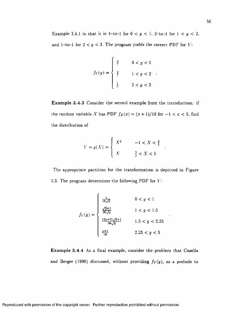
56

Example 3.4.1 in th a t it is 4 - to - l for 0 < y < 1. 2 - to - l for 1 < y < 2.

and 1 - t o - l for 2 < y < 3. T h e program yields the correct P D F for V':

f y (y ) =

0 < y < 1

1 < y < 2

2 < y < 3

E x a m p l e 3 .4 .3 Consider the second exam ple from the in troduction: if

the random variable .V has P D F / x ( x ) = ( x + 1 ) / lS for — 1 < x < 5, find

the d is tribu tion of

X-

X

- 1 < x < l

-y < X < 0

The appropria te parti t ion for the transform ation is depicted in Figure

3.3. The program determ ines the following P D F for V’:

f r ( y ) =

18,/v

36 /y

( 2 y + 3 ) ^ / y + \36 /y

U±i18

0 < y < 1

1 < y < 1.5

1.5 < y < 2.25

2.25 < y < 5

E x a m p l e 3 .4 .4 As a final exam ple, consider the problem th a t Casella

and Berger (1990) discussed, w ithout providing /y ( y ) , as a pre lude to

57

gfX)

5

4

3

0

- 1 0 I 2 3 4 5

Figure 3.3: T he transfo rm a tion V = g ( X ) has a discontinuity and is variously 1 - t o - l and 2 - to - l on different subsets of th e support of X .

their theorem . Letting .V be a uniform random variable on (0 ,2~ ) , find

the d is tr ibu tion of Y = <7 (.V) = sin 2 (.Y). As Figure 3.4 shows, this tran s

formation is 4 - t o - l for th e single V subinterval ( 0 . 1 ). Furtherm ore , since

n = 4. .Y ' = {0. f . Y - - 7r}- T he P D F of F is

M y ) = —7 = = t 0 < V < 1~Vy - r

which is com m only known as th e arcsin d is tribution (see Johnson, Kotz,

and B alak rishnan (1995. p. 212). To overcome the principal inverse diffi-

5S

g(X)

i.o

0. 5

0.0

Figure 3.4: T h e transform ation V' = g ( X) = s in 2 (A') for 0 < A' < 2~.

culty a lluded to in the previous section, the following equivalent s itua tion

has been devised: consider the random variable A’ ~ U( — f . j ) and let

Y' = g ( X ) = s in 2 (.Y). In this case the domain of A' will be the sam e as

the range of g ~ l which results from using the s tan d a rd arcsin function.

This so lu tion yielded a random variable with a notab le feature. T he dis-

f Y (y)t r ib u t io n ’s H F. hy(y ) = ----- — — , might be of interest to a reliability

1 - Fy{y)

engineer. For this d is tribu tion .

h Y {y) =V y - y 2 [*■ - 2 arcsin( 2 y - 1 )]

0 < y < 1 .

59

By plo tting this HF. one sees it has the rare p roperty of a closed-form.

“ba th tub~-shaped HF. Furtherm ore , one can now app ly the transfo rm a

tion W = g ( Y) = W in order to derive a random variable W th a t is a

one-param eter random variable w ith a closed-form. b a th tu b -sh a p e d HF.

Although th e arcsin d istribution has been discussed in th e li te ra tu re , there

appears to be no mention of the fact th a t it has a b a th tu b -sh ap ed HF.

Most d istr ibu tions with ba th tub-shaped hazard functions m ust be ana

lyzed numerically because their hazard functions are no t closed form. One

of the useful features of the T ra n s fo rm procedure is th a t it can help the

practitioner gain insight into w hat transform ations could result in a use

ful model. In this example, it becomes apparent th a t th e transform ation

"crowds” th e uniformly d is tr ibu ted A' random variable into a d is tr ibu

tion for Y th a t is “heavy’’ on e ither end of its suppo rt . T he result is a

random variable with a ba th tub -shaped hazard function. T he program

enables the model designer to confirm, or gain insight into the univariate

transform ations th a t could result in a useful model.

3.5 C onclusion

The tool provided by the T ra n s fo rm procedure will be useful to the p ractitioner as

well as the academic. T he academic might use this tool to find new distributions.

Let A' be a b e ta random variable w ith specified param eters , for exam ple, and let


60

g(A') = A"2. A pplying g several times in succession m ay yield a d is tribu tion th a t

is useful in modeling. Alternatively, s tuden ts might be asked to combine a set of

ten transform ations and ten distributions in order to c rea te 1 0 0 new distribu tions,

picking out the in teresting properties of the m ore no tab le ones.

The practitioner, on the other hand, m ay use the T ra n s fo rm procedure for the

specific purpose of iterative probabilistic model design, i l lus tra ted in Exam ple 3.4.4.

Examples provided in C hapter 7 use T r a n s f orm extensively.


C hapter 4

P rodu cts or R andom V ariables

4.1 In tro d u ctio n

Another keystone procedure is th a t of com puting th e p robab il i ty density function of

the p roduct of two independent random variables. T h e procedure P roductR V is very

useful for th a t purpose and is also em bedded in the SumRV procedure. R ohatg i 's well-

known result (1976. p. 141) for de term in ing the d is tr ib u tio n of the product of two

random variables is straightforward to derive, but difficult to im plem ent. Let .V and

Y be continuous random variables w ith jo int P D F f x y { x ~y)- T h e PD F of V” = X V

is

The im p lem en ta t ion of this result, however, is not s tra igh tfo rw ard for general A'

and Y . Difficulties occur as a result of both the m y riad varia tions to th e lim its of

integration an d th e propensity of th e P D F of V to be defined in a piece-wise m anner .

61


62

The cases when -V and V are independent and m ay have probability dens ity functions

defined in a piece-wise fashion are considered in this chapter. A ppendix F contains an

algorithm th a t handles these difficulties and is genesis for the p rocedure ProductRV.

4.2 T h eorem

A simple theo rem is presented in this section which illustrates some of the issues

associated with a general algorithm for determ in ing th e PD F of the p ro d u c t of two

independent ran d o m variables. For simplicity, assum e th a t the ran d o m variable ,V

has support on the interval (a.b) and the random variable has su p p o r t on the

interval (c . d ). Also, the p roduct space of the two random variables is assum ed to fall

entirely in the first quadran t .

T h e o r e m . Let X be a random variable of the continuous type with P D F f ( x ) which

is defined and positive on the interval (a.b). where 0 < a < b < oo. Similarly, let

be a random variable of the continuous ty p e with P D F g(y) which is defined and

positive on the interval (c, d). where 0 < c < d < oo. T h e P D F of V = X Y is

h(v) =

f a /e 9 ( ; ) f ( x ) ^ dx ac < v < ad

fv/d 9 ( j ) / ( * ) £ dx ad < v < be

. fv/d 9 ( r ) f ( x ) ^ d x be < v < bd

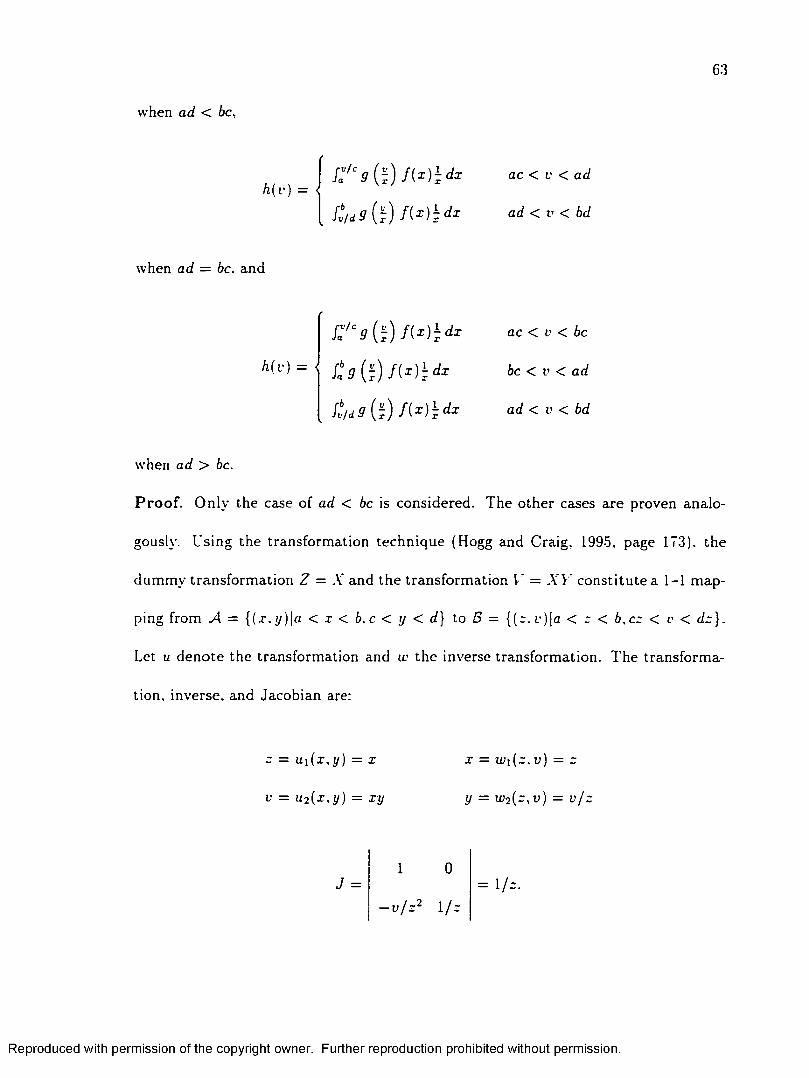
63

when ad < be.

h(v) = <fa /c 9 ( j ) / ( * ) £ dx ac < v < ad

when ad = be. and

Fa/C9 ( ; ) / ( * ) J ac < v < be

h[v) = < / ( x ) j dx be < v < ad

St/d 9 ( ]:) / ( * ) £ d x arf < y < 6d

when ad > be.

P r o o f . O nly the case of ad < be is considered. The o ther cases are proven analo

gously. Using the transform ation techn ique (Hogg and Craig. 1995. page 173). the

dum m y transfo rm ation Z = A" and th e transform ation V = .YV cons ti tu te a 1 - 1 m ap

ping from A = { (x .y ) |a < x < b.c < y < d} to S = {(x .c ) |a < z < b.cz < v < d.r}.

Let u d eno te the transform ation and w the inverse transform ation. T he transfo rm a

tion. inverse, and Jacobian are:

x = u i ( x , y ) = x x = wi ( z . v ) = z

v = u2{x, y) = xy y = w2( z , v ) = v / z

1 0J =

- v / z 2 l / z

64

T he jo in t P D F of Z and V is

f z . v (-* V) = f ( wi ( z , v) )g(w2(z . v) ) \J\ (=.v) e B ,

or/ z . r ( - . u ) = f ( = ) g ( v / z ) - (c, v) e B.

In tegra ting with respect to z over th e appropria te intervals and replacing c w ith x in

the final result vields

as desired.

h{ v) =

ac < v < ad

ad < v < be

be < v < bd

d

c xy = be xy = ad xy = ac

ba

Figure 4.1: The support of X and Y when ad < be.

6 5

V

bd

ad

ac

ba

Figure 4.2: T he m apping of Z = A' and V = X Y ' when ad < be.

T he geom etry associated with the transform ation is shown in F igures 4.1 and

4.2. Note th a t the transfo rm ation maps .4, onto for i = 1 .2 .3 . A lthough the

transfo rm ation techn ique has been used to prove this theorem , th e C D F technique

could also have been used.

4 .3 Im p lem en ta tio n

T h e theo rem in the previous section illustrates the im portance of considering the

m agn itudes of the p roduc t of th e coordinates of the sou theas t and no r th w es t corners

of th e p roduct space (e.g.. ( 6 , c) and (a .d ) ) when it lies en tirely in th e first q u ad ran t .

In o rder to apply the theorem to any continuous ran d o m variables X and V, th ree

generaliza tions need to be addressed.

66

1. Analogous theorem s m ust be w ritten for th e cases when th e {a.b) by {c.d)

rectangle lies wholly in one of the o ther th ree quadrants.

2. Instead of having probability density functions which are specified by a single

s tandard function over the ir entire suppo rt , th e random variables A' and Y may

be defined in a piece-wise m anner over several intervals, forming m any segments

to the PD F (e.g. th e tr iangular d is tr ibu tion).

3. T he cases when 0 and ± o c belong to the endpoin ts of the intervals which con

s t i tu te the support of A' and Y m ust be considered.

In fact, these generalizations result in 24 different cases th a t m ust be considered in

o rder to correctly com pu te the limits of in tegration of th e theorem. T he paragraphs

below address these cases. For quadran ts II. III. and IV. the limits of integration

m ust be set appropria te ly based on the geom etry of the transform ation .

For random variables th a t are defined piece-wise over various intervals, let n be

th e num ber of intervals for .A and let m be th e num ber of intervals for Y. There

are mn rectangular “p roduct spaces" and the con tribu tion of each to th e value of

the P D F of V = X Y m ust be com puted. Furtherm ore , each “p roduct space" can

con tr ibu te differently to th e P D F of V on up to th ree segments of the su p p o r t of V'.

As a result, the P D F of V tends to become com plica ted very quickly, w ith an upper

limit of 3m n segments to its P D F . For exam ple, th e p roduct of two U ( 0 ,1) random

variables yields a random variable V’ with only one segm ent (see E xam ple 4.4.1). But

w ith only a slight change, e.g., X ~ U( 1,2) an d Y ~ U (3 ,4), yields a V = X Y


67

defined differently on th ree segments (see Example 4.4.2).

T h e case where the support of a random variable contains 0 (e.g.. U( —1.2)) poses

special difficulty since some of the rectangular p roduct spaces will not lie wholly in

any one quadran t and cannot be handled by the previously developed techniques.

O ne solution to this difficulty is to add 0 as one of the endpoin ts of the intervals for

X and V' whenever this case occurs, producing redundan t segments, i.e.. two segm ents

on e i the r side of zero with the same formula for the P D F .

T h e algorithm consists of a set-up portion, followed by nested loops th a t de te rm ine

the con tribu tion to the P D F of V' = X Y separately for each of the four q uad ran ts .

A ppendix F contains the set-up portion and the a lgori thm associated with th e first

q u ad ran t . T he algorithm for the o the r quadran ts is similar.

T h e set-up phase begins by sett ing n and m to the num b er of intervals th a t form

the support of X and V'. Next. 0 is added as an interval delim iter for .V a n d /o r Y

if th e random variable can assume both positive and negative values, and 0 is not

a lready an interval delimiter. Finally, the endpoints of th e intervals which form the

su p p o r t of V are determ ined by taking all products of the endpoints of the A* intervals

tim es the endpoints of th e Y intervals.

A nested set of loops follows th a t trea ts all pairings of X and Y intervals. As shown

in F igure 4.1, the coordinates (a. c) are assigned to the southw est corner of the cu rren t

rectangle of interest, and the coordinates ( 6 . d) are assigned to the northeast corner

of th e curren t rectangle of interest. A tes t to de te rm ine which quadran t contains the

cu rren t rectangle is m ade a t this point. Adding 0 as an in terval delimiter in th e set-up


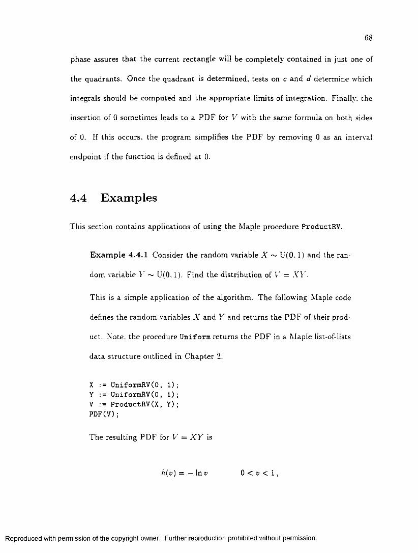
6S

phase assures th a t the current rectang le will be com pletely con ta ined in ju s t one of

the quadran ts . O nce the q uad ran t is determ ined , tests on c and d determ ine which

integrals should be com puted and the appropria te limits of in tegration . Finally, the

insertion of 0 som etim es leads to a P D F for V w ith the sam e form ula on both sides

of 0 . If this occurs, the program simplifies the P D F by rem oving 0 as an interval

endpoin t if the function is defined a t 0 .

4.4 E xam p les

This section contains applications of using the Maple procedure ProductRV.

E x a m p l e 4 .4 .1 Consider th e random variable .V ~ U ( 0 . 1) and the ran

dom variable Y ~ U (0 .1). F ind th e d is tr ibu tion of V = .YV’.

This is a simple application of the algorithm . T he following Maple code

defines the random variables A’ and Y and returns the P D F of their p rod

uct. Note, the procedure U n ifo rm re tu rns the P D F in a M aple list-of-lists

d a ta s tru c tu re outlined in C h ap te r 2.

X := UniformRV(0, 1) ;Y := UniformRV(0, 1);V := ProductRV(X, Y) ;PDF(V);

T he resulting P D F for V = X Y is

h(v) = — \ nv 0 < v < 1 ,

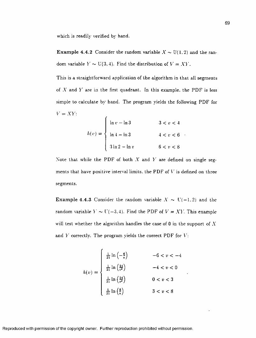
69

which is readily verified by hand.

E x a m p l e 4 .4 .2 C onsider the random variable X ~ U (1 .2) and th e ran

dom variable Y ~ U (3 .4 ) . Find the d is tr ibu tion of V’ = X Y .

This is a s tra igh tfo rw ard application of th e algorithm in th a t all segments

of A' and ¥ are in th e first quadran t. In this exam ple, the P D F is less

sim ple to ca lcu la te by hand. The program yields the following P D F for

Note th a t while th e P D F of both X and ¥ are defined on single seg

m ents tha t have positive interval limits, th e P D F of V’ is defined on three

segments.

E x a m p l e 4 .4 .3 C onsider the random variable .V ~ U( —1 . 2 ) and the

random variable ¥ ~ L*( — 3,4). Find the P D F of V = X Y . T h is exam ple

will test w hether th e algorithm handles th e case of 0 in the su p p o r t of A'

and ¥ correctly. T h e program yields the correct P D F for V':

V = X Y :

In v — In 3 3 < v < 4

h ( L') — { In 4 — In 3 4 < v < 6 •

3 In 2 — In v 6 < v < S

—6 < v < —4

h{ v) = <- 4 < v < 0

0 < v < 3

3 < v < 8

7 0

M aple returns a m athem atically equivalent P D F with a slightly different

functional form. M aple's calculation for th e first segment of V yields

j j l n ( 2 ) + j f ln (3 ) — jj-ln(c) + which reduces to the above first

segment, remembering th a t since v is negative in this segment ln (i’) =

ln( — 1 ) + ln( — c) = I t + ln( — v). so the im aginary portion cancels.

E x a m p l e 4 .4 .4 Consider the random variable X ~ tr iangu lar( 1. 2 .3)

and the random variable Y ~ t r i a n g u la r ( l ,2 .4 ) . Find the P D F of V =

.YV’. This non-uniform exam ple illustrates the case of several rec tangu la r

p roduct spaces. The M aple code in this case is:

X := T r i a n g u l a r R V ( l , 2, 3 ) ;Y := Tr iangularRVCl, 2, 4 ) ;V := ProductRV(X, Y ) ;PDF(V);

T he resulting PD F for I" has six segments:


71

—t f / 3 + 2 /3 In i' + 2 r /3 In v + 4 /3 I < v < 2

—8 + 14/3 In 2 + 7i;/3 In 2 + 10v/3 — 4 In v

—o r /3 In r 2 < r < 3

—4 + 14/3 In 2 + 7 r /3 In 2 + 2v — 2 In v

— r In r — 2 In 3 — 2 r /3 In 3 3 < v < 4

h { v ) = { 4 4 / 3 — 14 In 2 — 7 r /3 In 2 — Su/3 — 2 In 3

+ 2 2 /3 In v — 2 r /3 In 3 + 4 u /3 In v 4 < r < 6

8 /3 — 8 In 2 — 4t>/3 In 2 — 2u /3 + 4 /3 In v

+ r / 3 In v + 4 In 3 + v/ 3 In 3 6 < r < 8

—S + 8 In 2 + 2 r /3 In 2 + 2 r /3 + 4 In 3

—1 In v + v/3 In 3 — r / 3 In v 8 < r < 12

E x a m p l e 4 .4 .5 This exam ple illustrates the fact th a t the product of

two lognormal random variables has th e lognormal distribution. C on

sider the random variable A’ ~ L ogN (/ii . <rf) and the random variable

V ~ LogN(^ 2 - )• Find the PD F of V’ = AT". Here one sets / j i = = 0.

= 1 and <j \ — 4. The program yields the following PDF:

e - ( l nu)2/10h(v) = ------- 0 < v < oo .

e y i o ^

This can be identified as a LogN(/z = O.cr2 = 5) random variable.

E x a m p l e 4 .4 .6 Consider the random variable X ~ N ( 0 ,1) and the ran

dom variable V" ~ N (0 ,1). F ind the P D F of V = X Y . This will test the

case where the support of .V and V include the endpo in ts ± o c .

T he program yields the following P D F for V:

BesselK(0. v - signum(u))-------------------------------------- —oo < r < 0

h(v) = ,BesselK(0. e • s ignum (r))-------------------------------------- 0 < v < oc

' 7T

which relies on Maple's B e sse lK and signum functions. T h e M aple o u tp u t

of this func tion ’s plot is given in Figure 4.3.

f(x )

Figure 4.3: The P D F of V = X Y ’ for X ~ N ( 0 .1) and V ~ N( 0 , 1 ).

E x a m p l e 4 .4 .7 Consider the independent random variables U\ ~ U ( 0 , 1 )

and Ui ~ U(0. 1). T he B ox-M ulle r algorithm for gen era tin g a single

s ta n d a rd normal deviate V can be coded in one line (Devrove. 1996) as

V <— y j — 2 In U\ cos(27tU2),

where C\ and U2 are independen t random numbers. Using th e T ra n s fo rm

and P roductR V procedures toge ther , one can d e te rm in e th e PD F of W

Due to th e principle inverse difficulty with tr igonom etric functions, how

ever. th e transform ation m ust be rewritten as

U <— \ J In U\ cos( irU2 )

before using T ransfo rm .

T he p rogram yields the following P D F for V:

v r°

h(v) =

/*U v /I-*-

~ J - 1 \ / l - r

- /7T Jo

:2 x 21 e- f 2/(2*2)

dx —c» < u < 0

\ / l — X 2 X 2dx 0 < v < cc

W hile th is form in not easily recognizable as th e P D F for the norm al

d is tr ibu tion , it is m a them atica lly equivalent to th e m ore s tan d ard

I 2h(v) = —==.e~v ^ — oo < v < oc.

v 2tt

One an tic ipa tes th a t fu tu re generations of com pu te r a lgebra systems will

be ab le to simplify these integrals.

7 4

E x a m p l e 4 .4 .8 Devrove (1996) gives

A' <— m + (a + (b — a)U\ — m) m a x {£'2 , £"3 }

as a one-line algorithm for genera ting a tr iangular(a . m . b) variate. where

£'i. U2 . and £ 3 are independent an d identically d is tr ibu ted U ( 0 ,1) random

variables and the triangular d is tr ibu tion has a m in im um of a. a mode of

m. and a m axim um of b. O ne m ay now use this rela tionship to generate

the PD F of a random variable w ith th e triangular d is tr ibu tion . Using the

Maple procedure MaximumRV. which re tu rns the P D F of the m axim um of

two independent random variables and T ra n s fo rm for th e linear transfor

mations. one can derive the P D F w ith the following M aple commands.

a : = 1;m : = 2;b : = 3;U1 : = UniformRV(0, 1) ;U2 : = UniformRV(0, 1) ;U3 : = UniformRV(0, 1) ;T1 : = T ra n s fo rm (U l , [ [x -> a + (b

[ - i n f i n i t y , i n f i n i t y ] ] ) ;T2 : = MaximumRV(U2, U3) ;T3 : = ProductRV(Tl, T2) ;X : = Transform(T3, [[x -> m + x] ,

The resulting P D F for .V is:

/(*) =x — 1 1 < x < 2

3 — x 2 < u < 3

7 5

4.5 C onclusion

An a lgori thm for calculating the P D F of the p roduct of two independent random

variables X and Y' (which may be defined in a piece-wise manner) has been devel

oped and im plem ented. The A PPL procedure ProductRV is one of m any procedures

capable of au tom ating complicated probability calculations associated w ith random

variables. Potential application areas for calculations of this type include applied

s ta tis tics , biostatistics, goodness-of-fit, probabilistic modeling, renewal theory, relia

bility. sim ulation , and time series analysis.


C hapter 5

C om puting th e C D F of th e

K olm ogorov—Sm irnov Test S ta tistic

5.1 In trod u ction

A nother probabilistic p rob lem th a t is well su ited for co m pu ter a lgebra system s is

finding th e d istribu tion functions of th e K olm ogorov-Sm irnov te st s ta tis tic Dn in the

all-param eters-know n case. B irnbaum (1952) gives an n-fold in tegral for th e C D F

of th e te st s ta tis tic w hich yields a function defined in a piecew ise fashion, w here

each piece is a polynom ial of degree n. U nfortunately, it is difficult to d e te rm in e

the app rop ria te lim its of in teg ra tio n for com puting these polynom ials. T h e a lg o rith m

developed here (see A ppend ix G) perform s th e required in teg ra tions in a m an n er th a t

avoids calcu lating th e sam e in tegrals repeated ly , resu lting in sh o rte r co m p u ta tio n

tim e. It can be used to co m p u te th e en tire C D F or ju s t a po rtion of th e C D F , w hich

76


is m ore efficient for finding a critica l value or a p-value associated with a hypothesis

te st. T his approach yields exac t critical values and significance levels.

T h e K olm ogorov-Sm irnov (I\S ) test s ta tis tic D n, is defined by

D n = sup |F (x ) - Fn( x ) | .£

w here n is the sam ple size, F (x ) is a hypothesized C D F w ith fixed param eters, and

F n(x ). also called th e em pirica l d is tribu tion function, is a step-function th a t increases

by 1 /n a t each d a ta value. T his s ta tis tic has been used for goodness-of-fit te stin g

for continuous popu la tions for decades. T he KS te s t ’s appeal is its s traigh tfo rw ard

co m p u ta tio n of th e te s t s ta tis tic and the d istrib u tio n -free characteristic of D n. Its

d raw back is th a t its cu m u la tiv e d istribu tion function u nder the null hypothesis is

difficult to determ ine, leaving one to calculate critica l values w ith various app ro x i

m a tio n m ethods. C onsider th e d is tribu tion of the KS s ta tis tic in the case when all

p a ram eters are known.

B irnbaum (1952) gives th e C D F of D n — -C as

P ( ^ n < + L) = n! I ' " I * " ■un)dun . . . du2 dui“ 2 n t 2 n V 2 n V

for 0 < v < w here— in

g{u 1,«2.......... u„) = 1

78

for 0 < ui < u2 < ■ ■ ■ < u„ < 1. and is 0 otherw ise. Equivalently.

/ 1 \ r m i n d . ^ + v ) y m i n d . ^ + u ) y m i n d . ^ ^ i + i / )P [ D n < — + v ) = n! / / . . . 1 dun . . . du2 d u x.

\ -H / J m a x ( 0 , j j—u) Jmax(ui u) J m A x ( u „ - i . -u )

B irnbaum 's ra th e r harm less-looking integral is ted ious to com pute by hand , even for

sm all values of n. due to th e com plexity of th e region w here g is nonzero. E valuating

his expression requires calcu la ting many n-fold in teg ra ls whose lim its are de term ined

by considering a carefully chosen partition of th e su p p o rt of D n. T he difficult p a r t of

th e process is to set th e app rop ria te lim its on these integrals. T he final expression for

th e KS C D F is a piecewise polynom ial function in w hich each polynom ial has degree

5.2 L iterature review

T he lite ra tu re available on the KS s ta tis tic is ex tensive. S tephens’ a rtic le (C h ap te r

4 of D ’A gostino and S tephens. 1986) contains com prehensive coverage on th e use

of th e KS s ta tis tic , as well as o ther s ta tis tic s based on th e em pirical d is tr ib u tio n

function . He calcu la tes th e power of these goodness-of-fit tests. Johnson, K otz, and

B alak rishnan (1995, p. 640) consider this source (D ’A gostino, 1986) to be so com plete

th a t th ey have deleted I\S discussions in the ir second ed ition and refer th e read e r to

th a t com pendium instead . For com puting c ritica l po in ts of the KS d is trib u tio n , one

finds five-digit accuracy as early as 1956 (M iller, 1956). M iller relies on asy m p to tic

resu lts th a t converge fairly quickly to produce th e se estim ates. B irn b au m ’s a rtic le

79

(1952) also explains how various sets of recursive form ulas can be used to ca lcu la te

certa in critical po in ts to reasonable levels of accuracy. Law and K elton (1991. p.

3S7) ind icate th a t c ritica l points require com puter techniques, and are only easily

calcu la ted for n < 50. In the litera tu re there appea rs to be no source th a t produces

exact d is tribu tion functions for any d istribu tion w here n > 3. B irnbaum (1952. p. 441)

gives th e CD F of D n — ^ for n = 2 and n = 3. K n u th (1981) provides a functional

form for the C D Fs for th e two sta tistics D* and D ~ , b u t does not provide th e

CD F for Dn = m ax { D ^ . D~}. a harder problem given th e dependence betw een th e

two random variables. As a consequence of th e ap p a re n t com plexity of the requ ired

in tegration and lack o f lite ra tu re on exact d is trib u tio n s , it was apparen t early on th a t

a com putational a lg eb ra system , such as M aple, w ould be necessary to com pute th e

polynom ials needed for th e d istribu tion of the KS te s t s ta tis tic .

5.3 C o m p u tin g th e d istr ib u tion o f D n

W hen 0 < i’ < 2 ~. B irn b au m 's integral is easy to co m p u te since none of the intervals

of in tegration overlap. A dditionally , these intervals are all wholly contained w ith in

the in terval from 0 to 1. For exam ple. ut varies over th e in terval from ^ — v to ^ -4 - r .

and u2 varies over th e in terval from ^ — v to ■— + v. T h e in terval for u i begins to th e

right of 0 and ends before th e interval for u 2 begins. T h u s when 0 < v < th e lim its

of in tegration of B irn b a u m ’s integral guarantee th a t 0 < u : < u2 < ■ ■ • < u n < 1.

Because the u,'s are constra ined in this way, one m ay rep lace B irnbaum ’s in tegrand

g( u, \ , u2, . . . ,u n ) w ith 1. and thus com putation of th e KS C D F requires only a single

so

n-fold integral:

P ( Dn < -7 - + r') = nl [ [ 2n . . . f 2 1 dun . . . du2 du\ = ra!(*2 u)nV 2n ) J ± . .v J2Z=1-V

for 0 < v < d-.

W hen v has a fixed value g rea te r th an -C, it is also d esirab le to replace B irn b a u m ’s

in teg ran d by 1 . In o rd e r to ju s tify th is replacem ent, one m ust only allow in teg ra tion

over th a t region of n -d im ensional space for which 0 < u x < u2 5: ■ • • 5: un < 1-

Since th e intervals of in teg ra tio n specified in B irnbaum 's in teg ral for different u,'s can

overlap , the sm allest allow able value for any u, is influenced by all u / s w ith subsc rip ts

less th a n i th a t can ta k e on values in u ,’s interval of in teg ra tio n . This overlapp ing

requ ires partition ing th e in terval from ^ — v to _|_ v jn t 0 sub in tervals (w hich are

henceforth refered to as u -sub in tervals). w ith th e first u -su b in te rv a l s ta r tin g a t ^ — v

and a new u-subin terval beginning whenever the left en d p o in t of one of B irn b a u m ’s

in tervals of in teg ration is encountered . W hen any u, lies in a u-subin terval th a t

consists en tirely of negative values. B irnbaum 's in teg ran d is zero. For th is reason,

only u-subintervals th a t have a positive right endpo in t c o n trib u te to th e KS C D F.

O f course, the n u m b er of u-subin tervals th a t have a positive right en d p o in t de

pends on the value of v. For sm all values of v (i.e., 0 < v < ^ ) , n + 1 u -sub in terva ls

have a positive right endpo in t since all n of B irn b au m ’s lower lim its of in teg ra tio n

are positive. For large values of v (i.e., < v < on ly two u -sub in te rva ls

have a positive right en d p o in t since only un’s lower lim it of in teg ra tion is positive.

SI

In te rm ed ia te values of u produce all possibilities from 2 to n + 1 u-subintervals th a t

have a positive right en d p o in t.

B ecause different values o f u can yield different num bers of u-subintervals th a t

have a positive right en d p o in t, the interval 0 < v < ^£=1 m ust be subdivided a t the

following values of c: ^ ........~2 n^- ^ ^ e n th e values of u rem ain w ithin one

of th e resu lting sub in tervals for u. the num ber of u -sub in terva ls th a t have a positive

right en d p o in t will rem ain fixed.

A no ther com plication arises because it is necessary to know, for a fixed value of

r and for th e u -subin tervals p roduced by this value, w hich variables of in tegration u,

can take on values in each of the u-subintervals of [0,1]. T h e previous subdivision

of th e values of u is not fine enough to allow unam biguous specification of the range

for each u,. W hen i < j . u t, and u2 have overlapping in tervals of in tegration if

the u pper in teg ra tion lim it for u, exceeds the lower in teg ra tio n lim it for u2, i.e.,

+ v > - — t’- As a resu lt, as u increases from 0 to —. new overlaps takei n — i n 2n *

place when u equals d_. The interval 0 < u < m ust be d iv idedr 1 i n i n 2n i n i n

in to sub in te rva ls a t these values of v as well as a t th e values of v listed previously.

H enceforth these are refered to as u-subintervals.

In d ica to r m atrices will be used to sum m arize th e in terre la tio n sh ip s betw een th e

possible values for th e variables of in tegration u i , u 2, . . . , u n . For a fixed n and for

values of v in the Arth u-subinterval of th e in d ica to r m a trix Ak will show,

by th e presence of a 1 or a 0 in row i and colum n j , w h e th e r or not u, can take

on values in th e j th u-subin terval. F inally, by defining p a th s th ro u g h these ind ica to r

m atrices, one produces a com plete set of n-fold in tegrals which satisfy th e requ irem en t

0 < u : < u2 < • • • < un < 1. and which p roduce th e KS C D F when sum m ed.

T he algorithm for com puting th e cum ulative d is tr ib u tio n function of D n is d iv ided

into four phases. In Phase 1. an ap p ro p ria te p a r ti tio n of th e support of D n — ^ is

determ ined. In Phase 2. m atrices .4^ are defined th a t a re in s trum en ta l in d e term in ing

the lim its of in teg ration in th e n-fold in tegrals. In P hase 3. these integrals and th e ir

associated lim its are com puted . To take advan tage of th e sim ilarities in th e lim its of

in tegration of these rc-fold in tegrals, they are g rouped for efficiency and all evaluated

to the sam e level of in teg ration before proceeding to th e nex t level. Finally. P hase 4

consists of tran s la tin g th e support of Dn — ^ to th e su p p o rt of Dn. T hus th e in p u t

to the algorithm is a positive integer n and th e o u tp u t is the piecewise C D F of Dn.

5 . 3 . 1 P h a s e 1: P a r t i t i o n t h e s u p p o r t o f D „ - ^

The endpoin ts of the segm ents th a t define th e su p p o rt of the KS test s ta tis tic can

be determ ined from th e lim its of in tegration given by B irnbaum . I ’sing B irnbaum 's

formula, the baseline lower and upper lim its of in teg ra tion associated w ith u = 0 are

1 3 5 2 n — 12 n 2 n 2 n ' 2 n

As u increases, th e support of Dn — is broken in to disjo int u-subintervals. T he

endpoints of these support u-subintervals consist of v = 0 and the values o f v for

which th e endpoin ts of th e n intervals of in teg ra tio n e ither:

S3

• equal 0 or 1. or

• coincide.

T he 0 or 1 cases occur a t v values in the set

1 3 5 2n — 12n 2n 2n 2n

T he se t of values of v for which the endpoin ts of different intervals of in teg ra tio n

coincide are

r j _ _2_ _3_ n — 1 |12n 2n 'In' ’ 2n )

T hus th e union of th ese two sets and 0 com prise th e endpo in ts of th e u -sub in terva ls

of th e support of Dn —

T h e first phase of th e a lgorithm given in A ppendix G com putes th e above en d

points r 0 = 0. t’i . t ’ 2 t-m, where m is the num ber of u-subintervals on w hich the

C D F of Dn — is defined. For anv n.* 2n

'3 n lm = T - i .

5 . 3 . 2 P h a s e 2 : D e f i n e t h e A m a t r i c e s

At th is point in the a lgo rithm , uo, Ui___, um are th e endpo in ts of the m u-sub in terva ls

on w hich the CD F of D n — is defined.

Tw o book-keeping steps axe needed in this phase of th e algorithm . T h ey are:


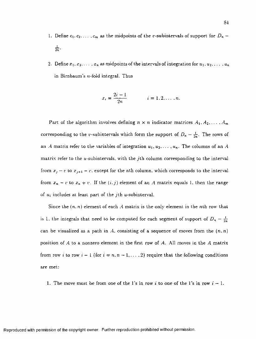
S4

1. Define c t .c 2..........cm as th e m idpoints of th e r-su b in te rv a ls of su p p o rt for D n —

i2 n *

2. Define X[. x 2......... x n as m idpoints of th e in tervals o f in teg ra tion for u t . u2.............un

in B irnbaum 's n-fold in tegral. Thus

2 i _ l • , 9x, = — ------------ i = 1 .2 n.2 77

P a rt of the a lgo rithm involves defining n x n in d ica to r m atrices A i .A 2 4 m

corresponding to the i’-subinter%rals which form th e su p p o rt of Dn — T h e rows of

an A m a trix refer to th e variables of in teg ration u i, u2 un . T he colum ns of an A

m a trix refer to th e u-subin tervals. w ith the jth. colum n corresponding to th e in terval

from i j — v to xJ+i — c. except for th e n th co lum n, w hich corresponds to th e in terval

from x n — r to x n + r. If th e ( i . j ) elem ent of an A m a trix equals 1. th en th e range

of u, includes a t least p art of the j t h u -sub in terval.

Since the ( n . n ) e lem ent of each A m atrix is th e only elem ent in the n th row th a t

is 1. th e integrals th a t need to be com puted for each segm ent of supp o rt of D n — ^

can be visualized as a p a th in A. consisting of a sequence of moves from th e ( n .n )

position of A to a nonzero elem ent in the first row of A. All moves in th e A m a trix

from row i to row i — 1 (for i = n , n — 1, . . . .2 ) requ ire th a t th e following cond itions

are m et:

1. T h e move m ust be from one of the l ’s in row i to one o f th e l ’s in row i — 1.


bo

2. T he move is e ith e r d irec tly vertical o r ve rtica l and one or more spaces to the

left.

T h a t is, if th e move begins a t a 1 elem ent in co lum n j of row i. it m ust end a t a 1

elem ent in colum n 1 th ro u g h j of row / — 1 .

E x a m p le 5 .3 .1 For n = 3 and k = 3. th e C D F is defined on the v-

subin terval | < v < | and has th e following ,43 m atrix :

A-i —

1 1 1

0 1 1

0 0 1

T here are five different paths from the (3. 3) elem ent to the top row of

the m atrix . In th e five m atrices below, th e se five pa th s to the top row of

the .4 m a trix are displayed by using boldface on th e path . N ext to each

m a trix is th e corresponding trip le in tegral th a t th e pa th represents.

1 L I

0 1 1

0 0 1

/ / / \ d u z d u 2 d u 1J 0 J l - v J±-v

1 1 1

0 1 1

0 0 1

/* g —u r - - u r l/ / 1 du3 du2dux

J - z - v J U l J ? - V

W hen th ese five integrals are sum m ed, B irnbaum 's expression reduces to

_ 1 \ , 11 11 2 3£>3 C - + 1 - ) - - J r + y " - 2 7 . 6 < r 6

N ote th a t th e inside integral

[ 1 du3 J U2

on th e th ird , fou rth , and fifth trip le in tegral is identical. T he n u m b er of

iden tical in teg ra ls of th is type grows rap id ly as n increases. T he a lg o rith m

developed here avoids recalculation of dup lica te integrals. C on tinu ing in

th is fashion for the o ther .4 m atrices (i.e., A\ , A 2, and A j), y ie lds the

N ote th a t B irnbaum (1952) contains a sign erro r in th e fo u rth r-su b in te rv a l

of support.

Table 5.1 shows how rapidly th e num ber of n-fold in teg ra tio n s requ ired to com pute

the C D F of Dn — ^ grows with n. N ote th a t th e five tr ip le in tegrals in the previous

exam ple corresponds to n = 3 and the th ird t>-subinterval (k = 3). show n in boldface

in the tab le. N ote th a t the fifth colum n in Table 5.1 is th e p ro d u c t of th e first and

fourth colum ns. T he fourth and fifth colum ns d id not m a tc h any well-known integer

sequences in the lite ra tu re (connect to

h t t p : //www. r e s e a r c h , a t t . c o m / ~ n j a s / s e q u e n c e s / i n d e x .h tml) .

Table 5.1: C om pu ta tional requirem ents for com puting th e D n C D F for sm all n.

n mN um ber of n-fold in tegrals required for each u-subinterval

T otal num ber of n-fold in tegrals

required

T o tal num ber of single integrals

required1 1 1 1 1

2 o 1 . 2 3 6

3 4 1. 4. 5. 3 13 394 5 1. S. 13. 9. 4 35 1405 7 1. 16. 34. 27. 28. 14, 5 125 6256 8 1. 32, 89. 81. 89. 48, 20. 6 366 2196


E x a m p le 5 .3 .2 T he m ethod for de term in ing th e in tegers in th e th ird

colum n of th e previous tab le is som ew hat analogous to de te rm in in g the

entries in a row of P asca l’s tr ian g le by using th e en tries of th e previous

row. B eginning a t each nonzero A m a trix elem ent in rows 2 through

n. th e re are a certa in num ber of p a th s whose m oves to th e top row of

the m a tr ix satisfy the tw o cond itions s ta te d previously. A ssigned to such

elem ents is a num ber p (for p a th s) th a t denotes th e n u m b er of p a th s from

th a t e lem ent to the top of th e m a tr ix . T hus if p2 2 = 2 (as is th e case for

the (2. 2) elem ent of the .43 m a tr ix for n = 3 and k = 3 in E xam ple 3.1)

then no m a tte r how one reached th is elem ent of th e A m a trix , th e re are

only two possible paths rem ain ing to th e top. T he p,,j values are assigned

as follows. O nly .4 m a trix e lem en ts w ith value 1 a re assigned a ptiJ value.

If the j th e n try in the first row of A is nonzero, assign pi.j = 1. For the

second and subsequent rows (i = 2 ,3 ...........n). pUJ = '£.q=iPi-i.q- F'pon

com pletion . pn.„ represents th e to ta l num ber of p a th s from th e lower right

corner of th e m a trix to th e top row of th e m atrix . C onsider, for exam ple,

the case of n = 5 and k = 4. T h e A m atrix w ith su p ersc rip ts denoting


89

the p,,j values is

0 l 1 l 1 l 1 0

0 l 1 l 2 l 3 l 3

A-i = 0 0 l 3 l 6 l 9

0 0 0 l 9 l 18

0 0 0 0 l 2 7

Here one sees th a t ps.s = 27. m eaning th e re are 27 possible paths to the

top row of A4 . consis ten t w ith the n = 5 and k = 4 elem ent in Table

o .l. T h e general a lg o rith m for com puting the num ber of paths for any

,4 -m atrix (provided as inpu t to the algorithm ) is as follows:

T o t S u m <— 0 p « - .4For i <— 2 t o n

For j <— / to n If = 0

Pi. j P i - i . j - i + p , ~ i , j else

Pi. j P i . j - i + P i - i . j Tot S u m *— Tot S u m + pnn

5 . 3 . 3 P h a s e 3 : S e t l i m i t s o n t h e a p p r o p r i a t e i n t e g r a l s

T he in d ica to r m a trix .4 shows, by the presence of a 1 in row i and colum n j . for

j < n . th a t u, can assum e values from the m axim um of Xj — t> and 0 to th e m in im um

of x J + 1 — v and x , + c. T h e presence of a 1 in row i and colum n n. m eans th a t u,

assum es values from x n — v to th e m inim um of x, + v an d 1 . Each p a th in A, as

described in Section 3.2. rep resen ts a set of allow able in tervals of in tegration for th e

90

variables U] to un in a p a rticu la r n-fold integral. For a p a rtic u la r path , the lim its

of in tegration for each u, are those given above th a t correspond to en try at J of .4

in row i th a t lies on th e p a th , w ith one exception: if bo th aUJ and a .- i^ are on the

sam e pa th , the lower lim it of in tegration for u, m ust be u ,_ i. T h is exception occurs

because the pa th allows u, and u,^i to assum e values in th e sam e u-subinterval. In

such a case, the lower lim it of in tegration for u, m ust be u ,_i in o rder to reflect the

requirem ent u,-_i < ut.

For each path th ro u g h th e m atrix A, and for each nonzero e n try a t J on th a t pa th ,

a single in tegration w ith respect to u; m ust be perform ed. If a ,_ ltJ is on the sam e

pa th as a tiJ, then th e lower lim it of in tegration will be the variab le u,-_i. If is not

on th e sam e pa th as a tJ , th en th e lower lim it of in teg ration will be a fixed num ber:

the m axim um of x : — v and 0. T hus for each p a th which passes through a;,j. e ither

a variable or fixed lower lim it of in tegration m ight be ap p ro p ria te .

E x a m p le 5 .3 .3 C onsider again the case of n = 5 and the fourth v-

subin terval (k = 4). T he A4 m atrix shown below has its l 's replaced

w ith T \ V. or B. ind icating w hether a fixed-lim it in teg ra l, a variable-lim it

91

in tegral, or both need to be com puted for each entry .

A , =

0 T T 7 0

0 V B B T

0 0 B B B

0 0 0 B B

0 0 0 0 B

In general, when the .4 m a trix con tains a zero, n e ith er th e fixed nor variab le lower

lim its need to be com puted . Now consider th e e lem ents of th e .4 m a trix th a t contain

a 1. T he positions associated w ith th e first 1 in each co lum n of .4 requ ire only a

fixed lower lim it to be calcu la ted . T he positions below th e first 1 in th e first nonzero

colum n require only a variable lower lim it to be calcu la ted . All o th e r positions in

th e .4 m a trix associated w ith 1 elem ents require b o th a fixed a variable lower lim it

to be calcu la ted . Table 5.2 shows the com p u ta tio n a l efficiency of perform ing th e

in teg rations for various values of n by using the algo rithm . T he num ber of single

in tegrals (algorithm ) for any n is bounded above by

n(n + 1)

w here th e first factor corresponds to th e m axim um num ber of l ’s in any A m a trix , th e

second factor accounts for co m pu ting bo th th e fixed and variab le m atrices (described

subsequen tly ), and th e last facto r is one less th a n m since no in teg ra tio n is requ ired


92

T able 5.2: C o m p u ta tio n a l efficiency associated w ith using the F and V' arrays.

n mTotal n um ber

of single in teg rals required (T able 5.1)

Total num ber of single integrals

required (algorithm )1 1 1 02 2 6 43 4 39 234 5 140 485 7 625 1086 S 2196 17010 14 442540 80015 22 318612735 279320 29 232093052440 640030 44 136617382366486800 2155050 74 61056379955994182386843138150 99500

for th e first r-su b in terva l. D ue to savings associa ted w ith 0 columns in the A m a trix

and th e fact th a t bo th fixed and variable m a trix elem ents do not need to be ca lcu la ted

in all cases, th is order n 3 expression is closely approx im ated by O.SOn3 for n = 20, 30,

and 50.

T ab le 5.3 on page 101 lists the coefficients of th e polynom ials th a t define th e

C D F of D n — ^ as com puted by the a lg o rith m in th e A ppendix which has been

im p lem en ted in M aple for n = 1 .2 . . . . ,6 . T h e ab ility to store fractions ex ac tly is of

p a r tic u la r benefit for these calculations. R a th e r th a n deta il every aspect of th e logic

of P h ase 3 of th e a lgo rithm , illu s tra ted below is th e evolution of th e n x n m a trices F

(for fixed lim its) and V (for variable lim its) in a row-by-row fashion for a p a r tic u la r

com b in atio n of n and k.


93

E xam ple 5 .3 .4 C onsider again th e case of n = 3 and k = 3. which

corresponds to th e u-subinterval | < r < | . T he x, values associated

with n = 3 are x j = g, x 2 = | . and x 3 = | . T he t \ values associa ted w ith

n = 3 are vq = 0. Vi = t>2 = | . v3 = and u4 = | . T he cen ters of the

v-subintervals a re cx = c2 = c3 = and c4 = 5 . T h e A 3 m atrix

is

<43 =

1 1 1

0 1 1

0 0 1

The F and I ’ m a trices are com puted sim ultaneously, row by row, s ta rtin g

with th e last row and ending w ith th e first. Thus all of th e elem ents of

the th ird row of F and of I ’ are com puted before com puting th e elem ents

of the second row is begun. In general, integrals which are calcu la ted

in a p a rticu la r row becom e in tegrand candidates for the in teg ra tion to

be carried ou t in th e row im m ediately above. T he F and V m atrices

are designed to s to re th e in te rm ed ia te resu lts of in tegration of th e n-fold

integrals so th a t th e necessary inner in teg ra tion operations a re perform ed

only once. E n tries in th e zth rows of F and V each resu lt from n + 1 — i

single in teg ra tio n s, one in tegration corresponding to th e ith row and one

in tegration for every lower row. T h e F m a trix stores the resu lts of all

in tegration in w hich th e last in tegral had a fixed lower lim it and th e V

m atrix sto res th e resu lts of all in teg ra tion in which th e last in teg ra l had

94

a variable lower lim it. In this exam ple, for th e inner-m ost in teg ra tio n

variable u3. th e re is only one possible fixed in tegration to com pute a n d one

possible variab le in teg ra tion to com pute on th e th ird u-subin terval. T hese

com putations are seen in th e (3. 3) elem ent of th e respective m atrices:

Fui F u2 Fl. 3 Vi.i 1.2 I’ 1.3

F = 0 F2.2 F2.3 V = 0 ^2,2 ^2,3

0 0 / L , Idu3 0 0 J i ld u 3 _

T he second variab le . u2. has four possible com binations of lim its and in te

grands. T hus th e re are four storage elem ents for u 2, found in the second

rows of the F and \~ m atrices. E lem ents (2. 2) and (2. 3) of th e F

m atrix store in teg ra tio n results th a t have all fixed lower-lim its of in teg ra

tion. bu t th e in teg rands are fixed and variable, respectively. S im ilarly ,

elem ents (2. 2) and (2. 3) of the I ' m a trix are for th e cases w hen the

lower-limit of in teg ra tion contains the u t variable, while th e in teg rands

are fixed and variab le, respectively. F2-2 is com puted to cover th e case in

which uo varies over th e second u-subinterval and u3 varies over th e th ird

u-subinterval. F 2.3 covers th e case in which both u 2 and u3 vary over th e

th ird u -sub in terval. so u3 m ust have u 2 as its variable lower lim it: hence

th e in tegrand is V3-3, not F3,3. Sim ilar cases are covered by V2<2 and V2>3,

except th a t variab le lower lim its are used in an tic ipa tion of th e fact th a t

u t and u 2 can b o th vary over the sam e u-subin terval, m aking it necessary

to have Ui as th e (variable) lower lim it for u 2. T he in tegrations in th e

95

second row of each m a trix are shown below (no te, th e in teg ra tio n for the

(3, 3) e lem en t, previously discussed, has been carried out}.

Fl .l A . 2 -Fi.3

0 0

W .l W ,2 W ,3

V’ = 0 f l ~ v F3'3 du2 f u\ +vV3'3du2

0 0 1 — u2

For the th ird and last variable, u t , on ly fixed-lim it in teg ration takes place

so only th e F m a trix gets updated . T h e (1 .1 ) elem ent covers th e case in

which U\ varies over th e first u-subin terval and u 2 varies over th e second

and th ird u-subin terval. T he (1. 2) e lem en t covers th e case in which U!

varies over th e second u-subinterval an d u2 varies over the second and

th ird u-sub in terval. T he (1. 3) elem ent allows bo th ui and u2 to vary over

the th ird u -sub in terval. T he integrals in th is first row are shown below

(note again, all previously discussed in teg ra tio n have been carried out in

the second and th ird rows of F and V'):

F = 0

0 0


96

V'i.i

0 0

T he com plete ly evaluated F m a tr ix is given by

F = 0 9 X 3^

0 0

Finally, th e C D F on the 3rd e-sub in terval is th e sum of the elem ents in

the first row of the F m atrix , all m ultip lied by 3! = 6.

5 . 3 . 4 P h a s e 4 : S h i f t t h e d i s t r i b u t i o n

At th is po in t, th e C D F is com puted in th e form P {D n < v + -A). Now one converts

th e d is tr ib u tio n in to th e more usable form P { D n < y) = F bn(y) by m aking th e

su b s titu tio n y = v + A- jn both th e polynom ials and th e u-subintervals of th e C D F.

Specifically, one adds — to each en d p o in t of th e u-subintervals and one su b s titu te s

{y — for d in th e C D F polynom ials. O ne then takes these two lists of num bers

and polynom ials respectively, sim plifies th em (using M aple 's s i m p l i f y ( ) co m m and),

and creates th e C D F rep resen ta tion in th e form of th e “list-of-lists” rep resen ta tio n

for d is tr ib u tio n s ou tlined in C h ap te r 2. T his enables us to use th e d is tr ib u tio n in th e

ways th a t all o th e r d is tribu tions are used in A P P L . Specifically, one can now verify

9 7

critical values for th e d is tribu tion , bu t more im portantly , one can calcu la te exact

significance levels of any given s ta tis tic . An exam ple of th e sh ifted d istrib u tio n for

n = 6 is:

FDe(y) =

0

460S0 y6 - 23040 i/5 + 4800 +

2S80 y 6 - 4800 y 5 4- 2360 y4 - y3 + 2§* y2 + g y - ±

320 y6 + 320 y5 - ^ y* - ^ y - ^ - 6

-2 S 0 y 6 + 560 y5 - ^ y * + y3 + lf3S y * _ ^ y + A

104 y6 - 240 y -5 + 295 y4 - y3 + & y2 - ^ y + £

- 2 0 y 6 + 3 2 y 5 - - f y3 + ^ y 2 + ^ y - l

10 y6 - 38 y5 + I f V - - {M y 2 + y - 1

—2 y6 + 12 y5 - 30 y4 + 40 y3 - 30 y2 + 12 y - 1

1

U < n

h ^ y < \

£ < y < t

\ < y < h

\ < y < h

n < y i

The M aple P l o t D i s t o u tp u t of the C D F and PD F of D& are show n in F igure 5.1 and

Figure 5.2. T h e com m ands used in M aple to produce these p lo ts are:

Y := KSRV(6);P lo tD is t (C D F (Y ) , 0, 1);P lo tD i s t ( P D F (Y ) , 0 , 1);

Note th a t th e re is a d iscontinuity in th e PD F at y = and m ore generally, a t

y = K T h is corresponds to th e value v = ^ in B irn b au m ’s orig inal integral.

This is th e sm allest value of v for which the n-dim ensional h y p ercu b e centered a t

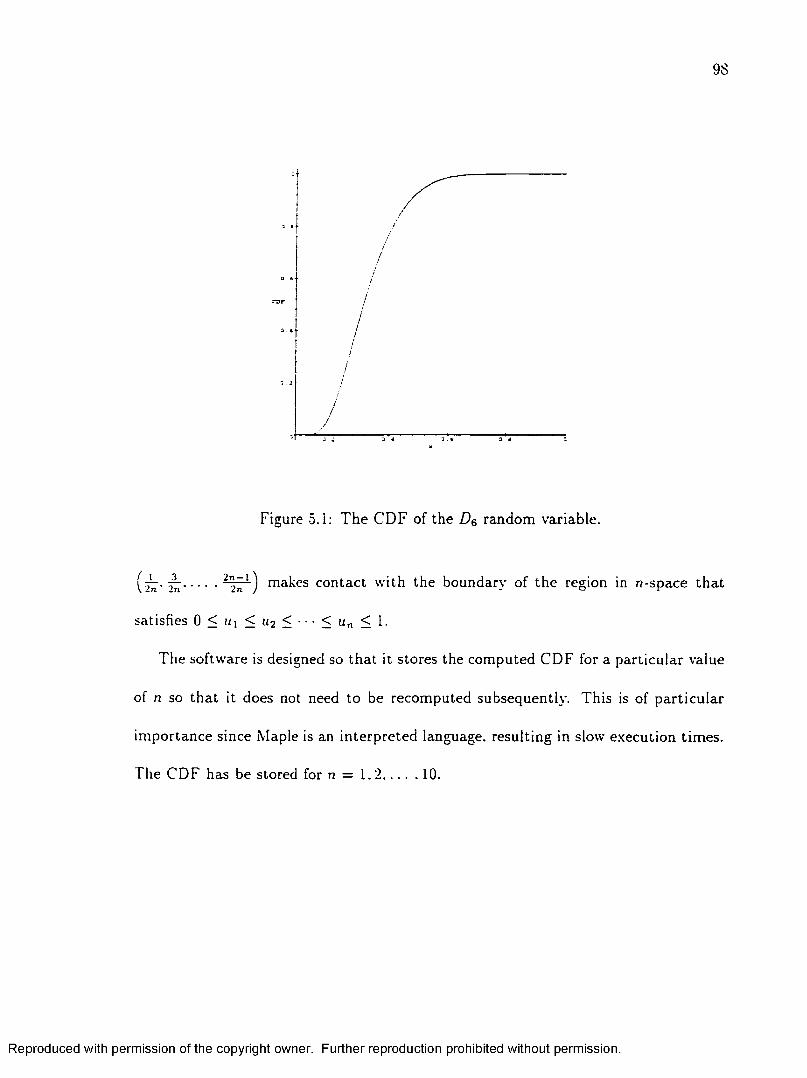
9S

Figure 5.1: T h e C D F of the D6 random variable.

( ^ . ^ ......... ^ 2 n^) m a^es con tac t w ith th e boundary of th e region in n-space th a t

satisfies 0 < < u2 < • • • < un < 1.

T he softw are is designed so th a t it stores the com puted C D F for a p a rticu la r value

of n so th a t it does not need to be recom puted subsequently . This is of p a rticu la r

im portance since M aple is an in te rp re te d language, resu lting in slow execution tim es.

The C D F has be stored for n = 1 .2 ..........10.

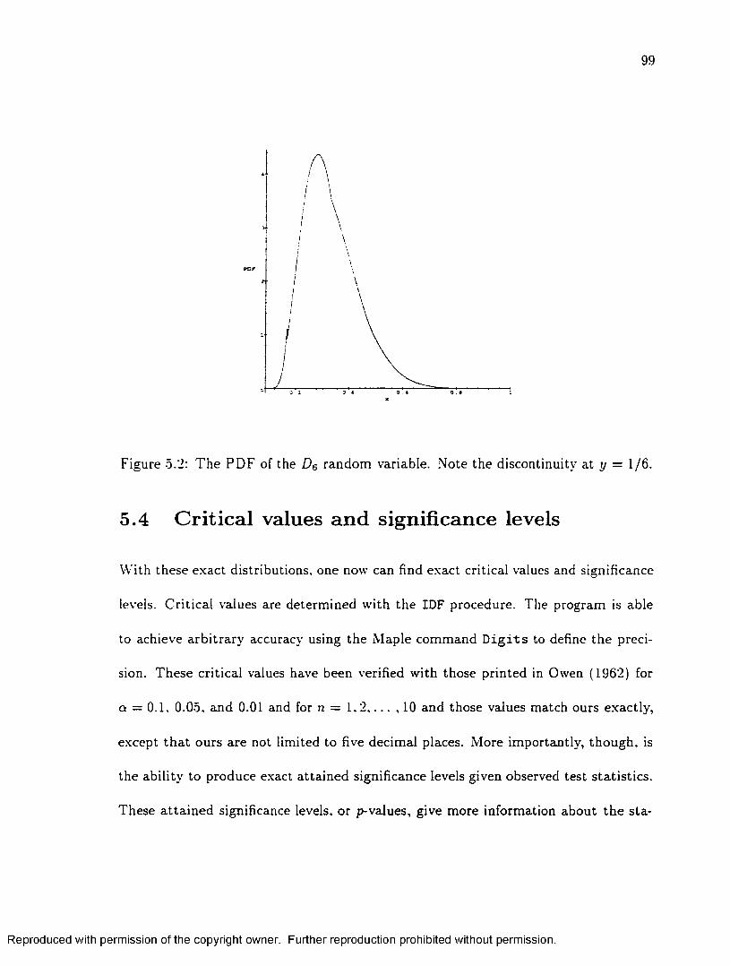
99

Figure 5.2: T h e P D F of the Z)6 ran d o m variable. N ote th e d iscontinuity a t y = 1/6.

5.4 C ritica l values an d sign ifican ce levels

W ith th ese exac t d is tribu tions, one now can find exact critica l values and significance

levels. C ritica l values are determ ined w ith th e IDF procedure. The program is ab le

to achieve a rb itra ry accuracy using th e M aple com m and D i g i t s to define th e preci

sion. T hese critica l values have been verified w ith those p rin ted in Owen (1962) for

or = 0.1. 0.05, and 0.01 and for n = 1 , 2 , . . . ,10 and those values m atch ours exac tly ,

except th a t ours are not lim ited to five decim al places. M ore im portan tly , th o u g h , is

th e ab ility to p roduce exact a tta in e d significance levels given observed te st s ta tis tic s .

T hese a t ta in e d significance levels, o r p-values, give m ore inform ation ab o u t th e s ta


100

tistica l te s t of hypothesis th a n does th e trad itio n a l “accep t/re jec t" regions associated

w ith critica l values. Using the p rocedu re CDF(). one can find these exac t significance

levels. For exam ple, let n = 6 an d th e observed te st s ta tis tic D& = 0.5543. Tw o c r it

ical values are, for exam ple. 0.51963 for a = 0.05 and 0.61661 for a = 0.01. O ne can

now d e te rm in e th e exact a t ta in e d significance level of the te s t s ta tis tic w ith the com

m and 1 - CDF(D6, 0 .5 5 4 3 ). which yields a p-value of 0.02928, a c learer ind ica to r of

the level of evidence against Ho. N ote th a t it is not necessary to co m p u te th e en tire

Dn d is tr ib u tio n to ob ta in a p a rtic u la r significance level. O ne m ust only determ ine

which segm ent of support the s ta t is tic belongs to . then execute th e a lgo rithm for ju s t

th a t piece of th e C D F. T h is sh o rtc u t will reduce th e integral co m p u ta tio n tim e by

approx im ate ly -100%. w here th e exac t savings depends on th e e-sub in terval th a t

is chosen. T able 5.1 indicates th a t th e g rea tes t tim e savings will p robab ly be in the

tails of th e d is trib u tio n . T his tim e savings is particu la rly im p o rtan t for larger values

of n.

5.5 C on clu sion

An a lg o rith m for com puting th e C D F of th e KS te st s ta tis tic in th e a ll-param eters-

known case for a positive in teger p a ram ete r n has been p resen ted . C om puting the

CD F provides a challenging calcu lus problem , even for sm all values of n. T h e C D F

can be co n stru c ted from a set of piecewise degree-n polynom ials. T h e a lg o rith m can

be used to plot the CD F or to ju s t find p a rticu la r fractiles or p robab ilities.


101

Table 5.3: C D Fs of D n — for n = 1 ,2 ...........6.

n m k Coefficients of C D F polynomials Subinterval

1 1 1 2.0 0 < v < In2 2 1 8 , 0 .0 0 < V < 1

4

2 - 2 . 3 . i4 < V < 3

4

3 4 1 4 8 . 0 ,0 , 0 0 < V < 16

2 - 1 2 . 8 , 1 . - ! I6 < V < 2

63 - 4 . 0 - U 2

6 < V < 36

4 2 - 5 - - — *■' J’ 6 ’ 10836 < V < 5

6

4 5 1 3 8 4 . 0 . 0 , 0 , 0 0 < V < 18

2 18. 0, 15, - | i 256i8 < V < 2

8

3 1 6 . - 4 0 , 2 1 . - 1 , - ^ 28 < V < 3

84 - 27 293 853

' • 1 6 ’ 64 • 204838 < V < 5

8- ^ - 147 343 353 5

< V <7

‘ ■ 16 ’ 64 ’ 2048 8 8

5 i 1 3 8 4 0 . 0 , 0 . 0 , 0 . 0 0 < V < 110

2 n Ofifi 96 36 6 U , 2 0 8 , - . 2 5 . 1 2 5 '6 2 5110 < V <

2To

3 160 - 1 6 0 — — - — — i u u . i u u . 5 , 2 5 ' 1 2 5 ’ 1252

To < V < 310

4 9 f l 6 4 318 542 343 273 ^ u . u -t . - , 25 , 500, 1250 310 < V < 4

105 , 9 n 62 6 2391 3413

L- ' u ’ 5 ’ 5 ’ 500 ’ 62504 < V < 510 10

6 o i o 52 19 1838 10527 ° * i 0 ’ 5 ’ 5 ’ 250 ’ 25000

510 < V < To

- o n 81 729 6561 9 049 “ • 5 ’ 50 ’ 1 0 0 0 ’ 50000

7< V <

91 0 10

6 8 1 4 6 0 8 0 . 0 . 0 . 0 . 0 . 0 . 0 0 < V < 112

2 2880. - 3 3 6 0 . 6 6 0 .6 0 . - f § , & . - 5 ^ 41

12 < V < 212

3 3 2 0 . 4 8 0 . - 7 0 0 . - ^ . - 2 2 , ^ 2IT? < V < 3

124 ■ io n t o n 335 1675 26005 3125 20645

2 , 54 • 864 ’ 1 7 2 8 ’ 3 7 3 2 4 8312 < V < 4

125 i n i t o o 1235 7435 36245 7 327 6 9 7 9 7

lO O . 6 , 54 i 864 ’ 5 1 8 4 ’ 3 7 3 2 4 8412 < V < 5

126 o n o n 45 2005 185 57971 4 0 6 4 6 9

^U, 4 , 1Q8 , 1 7 2 8 ’ 10368 ’ 7 4 6 4 9 6512 < V < TI

- If! 925 3065 22175 134 807 6 3 2 8 6 3 1U. OO, 24 , 216 , MS6 , 20-36 , j4 9 2 9 9 27

V < 912 12

8 o i i 605 6655 73205 161051 2 7 8 5 6 9 i i , 24 ’ 216 ’ 3456 ’ 20736 ’ 1 4 9 2992

9 V < 1112 12

C hapter 6

G oodness o f F it using Order

Statistics

6.1 In trod u ction

P resen ted in this chap ter is a detailed application of A PP L in which a new goodness-

of-fit te st s ta tis tic is devised. T he inception and im plem entation of th is te s t is possible

p rim arily due to th e ex istence of A PPL. This app lication highlights how th e parad igm

of p rob lem solving shifts w ith th e advent of a p robab ility language. P resen ted here

is a new m ethod of using o rder s ta tis tics for judg ing th e fit of d a ta by a hypo thesized

d is trib u tio n . T here is a variety of uses of o rd er s ta tis tic s in s ta tis tic a l inference

procedures. One reason is th e po ten tial for ad ap tin g such procedures for use w ith

censored sam ples (Cox and O akes, 19S4 and D avid, 1993). O ther app lica tions concern

behav ior in the tails of a paren t d istribu tion (for exam ple, o u tlie r te s ts , T ie tjen ,

102


103

1986). s itua tions in w hich the ordered d a ta are collected over tim e (life te stin g , for

exam ple, Barlow and P roschan . 1975). and estim ation of p aram eters in te rm s o f linear

com binations of o rder s ta tis tic s (D avid. 1993). A laxge lite ra tu re on th e su b je c t ex ists

(see, for exam ple D avid. 1981 and references cited there in ).

O ne im p o rtan t class of problem s involving o rder s ta tis tic s is goodness-of-fit te s t

ing (D ’A gostino and S tephens, 1986). T he S hap iro -W ilks no rm ality te s t (Johnson

and W ichern. 1992. p. 158) is based on a s ta tis tic th a t uses, in p a rt, th e ex p ec ted

value of each o rder s ta tis tic . Since many of th e te sts com m only used are defined

th rough the sam ple d is tr ib u tio n function, they m ay be considered to b e functions of

th e underlying o rder s ta tis tic s . It is com m on practice to transfo rm o rd e r s ta tis tic s

from a parent p opu la tion for the continuous random variable X w ith cu m u la tiv e d is

trib u tio n function F to corresponding U(0, 1) o rder s ta tis tic s , th rough th e p ro b ab ility

integral tran sfo rm a tio n , V = F [X ) . If the proposed te st s ta tis tic is in v a rian t u nder

th is transfo rm ation , it follows th a t its d is tribu tion m ay be derived for th e case of a

U(0. 1) paren t d is tr ib u tio n , and applied for any o th e r continuous p a ren t d is tr ib u tio n .

T h a t is. the p rocedure in this case is ‘‘'d istribu tion free.”

An exam ple of th e foregoing is th e K olm ogorov-Sm irnov ( I \-S ) one-sam ple te s t ,

based on the te s t s ta t is tic Dn = supx |F (x ) — F „ (x ) |, w here Fn is th e sam p le d is tr ib u

tion function. Since th e norm is invariant under transfo rm ations on x , it follows

th a t one m ay find c ritica l values for D n using th e d is trib u tio n of m a x ,{ m a x { |u t —

|t£, — ^ |}} , w here u, = F (x ( ,) ) ,i = 1 ,2 , . . . ,n . Following th e d evelopm en t of

th e K -S te st, m any a rtic les adap ted the te st to re la ted o rder s ta tis tic -b a se d te sts :


104

te sts for d a ta on a circle (K u iper, 1960 and S tephens, 1965). te sts w ith p aram eters

es tim ated from d a ta (L illiefors. 1967 and 1969), te s ts for censored sam ples (B arr and

D avidson. 1973). and o the rs . In addition to its use in non-param etric goodness-of-fit

te sting , th e K -S p rocedu re m ay be used in a general way to ob ta in confidence re

gions for p a ram ete r vectors (B a rr and D avidson, 1973); in terestingly , th e la tte r is a

p aram etric problem .

In Section 6.2 a vector of U(0. 1) s ta tis tics is defined by transform ing th e o rder

s ta tis tic s th rough each of th e n hypothesized C D Fs. Also suggested are possible uses

of th e vector in a varie ty of s ta tis tic a l problem s, an d it is shown how' th e m arginal

d is trib u tio n s of its com ponen ts can be com puted w ith m a th em atica l softw are such

as M aple. These ideas a re applied to define a goodness-of-fit s ta tis tic and sim ulation

is used to show it is adm issib le relative to th e K -S and A nderson-D arling tests in

Section 6.3. Possible ex tensions and conclusions a re given in Section 6.4.

6.2 T h e P -v e c to r

Proposed here is a m easure of th e goodness-of-fit of em pirica l d a ta by a hy p o th

esized d is trib u tio n based on th e vector of real num bers called th e "P-vector. Let

A 'i, A*2 , . . . . An be a ran d o m sam ple from a popu la tion w ith continuous C D F F , and

let A (1),A '(2 ) , . . . .A'(„) be th e corresponding o rd er s ta tis tic s . T hen th e ind iv idual


1 0 5

order statistics have marginal densities / x (l,(^). /a'(2)(x )’ • • • ' fx{n)ix ) given by

fx- ' [z) = ( , _

w here / a'(x ) = P\-(x ) (see Larsen and M arx. 1986, for exam ple). In princip le , one

can use these d is trib u tio n s to determ ine th e quan tiles for each ordered observation in

its respective d is trib u tio n . Define the P -v e c to r to be the n-vector

V = [F Y(n(-r(l)).^A'(2)(^(2))...........^ , B)(X(n))]-

For sim plicity in n o ta tio n , let p, = Fxit)(x(i) ) J = 1 .2 n. In tuitively , poor fit is

ind icated by "extrem e" com ponents in P . T hus, under the null hypothesis Hq: A has

C D F Fx{x) w ith n = 3 observations, for exam ple, a P -v ec to r of [0.453.0.267.0.623]

in tu itively indicates a good fit more so th an a P -v ec to r of [0.001.0.005.0.997].

Since th e individual e lem ents p, are th e resu lt of the probability in tegral tra n s

form ation. it is clear th a t P, ~ f/(0 . l ) . i = 1 .2 n. for any continuous popu la tion

C D F F. W hile th e P, a re identically d is trib u ted , they are not stochastically indepen

dent. T here is positive au tocorre la tion am ongst elem ents of the P -v ecto r.

T he P -v ec to r has a num ber of po ten tia l uses as a basis for d is tribu tion -free s ta t is

tical procedures. It can provide a d is tribu tion -free tool to identify ou tliers. T ie tjen

(1986. p. 497) m entions in his paper on outliers “We shall discuss here only th e un

derlying assum ption of no rm ality since the re is very little theory for any o th e r case".

As is discuss below, it is possible and p ractical to calcu la te all pi for nearly any hy


106

pothesized continuous d istribu tion , so one m ay use th e "P-vector as a basis to identify

outliers from any specified continuous d is tr ib u tio n . As one approach , one could ex

am ine th e first and last few elem ents of P (p\ and p„, for exam ple) to de te rm in e

w hether they are s ta tis tic a lly significant. Also envisioned are uses of th e P -v e c to r

for s ta tis tic a l inferences involving censored sam pling and estim ation based on "order

agreem ent." T he m ain application investigated here is goodness-of-fit te s tin g using

te st s ta tis tic s based on th e P -vector.

6.3 Im proving com p u ta tion o f V

C om puting the elem ents of th e P -v ec to r can be accom plished w ith A PPL . T h e pro

cedure OrderSta tCX, n , r ) for exam ple, determ ines the d istribu tion of th e r Lh out

of n o rder sta tis tics. Com bined with th e p rocedu re CDF(X, x). w hich re tu rn s Fx{x)-

the elem ents p, are calcu lated .

It is preferable to calcu la te the P -v e c to r by first transform ing to U(0, 1) o rder

s ta tis tic s , and then determ in ing the quan tiles p, using corresponding b e ta (i. n — / + 1)

C’D Fs. which are rela tively sim ple polynom ials as ind icated in F igure 6.1. T h e calcu

lation of pi = F y(i) (£(,)) as first described is dep ic ted by th e path shown by a solid line

in F igure 6.1. This m ethod of com putation relies on th e ability to ca lcu la te quan tiles

in d is tribu tions of all of the order s ta tis tic s X ^) , a lthough recurrence re la tions for

C D Fs of order s ta tis tic s m ight speed co m p u ta tio n (D avid, 1993). T h e second ap

proach. using b e ta C D Fs, is depicted by th e dashed line in F igure 6.1. It requires the


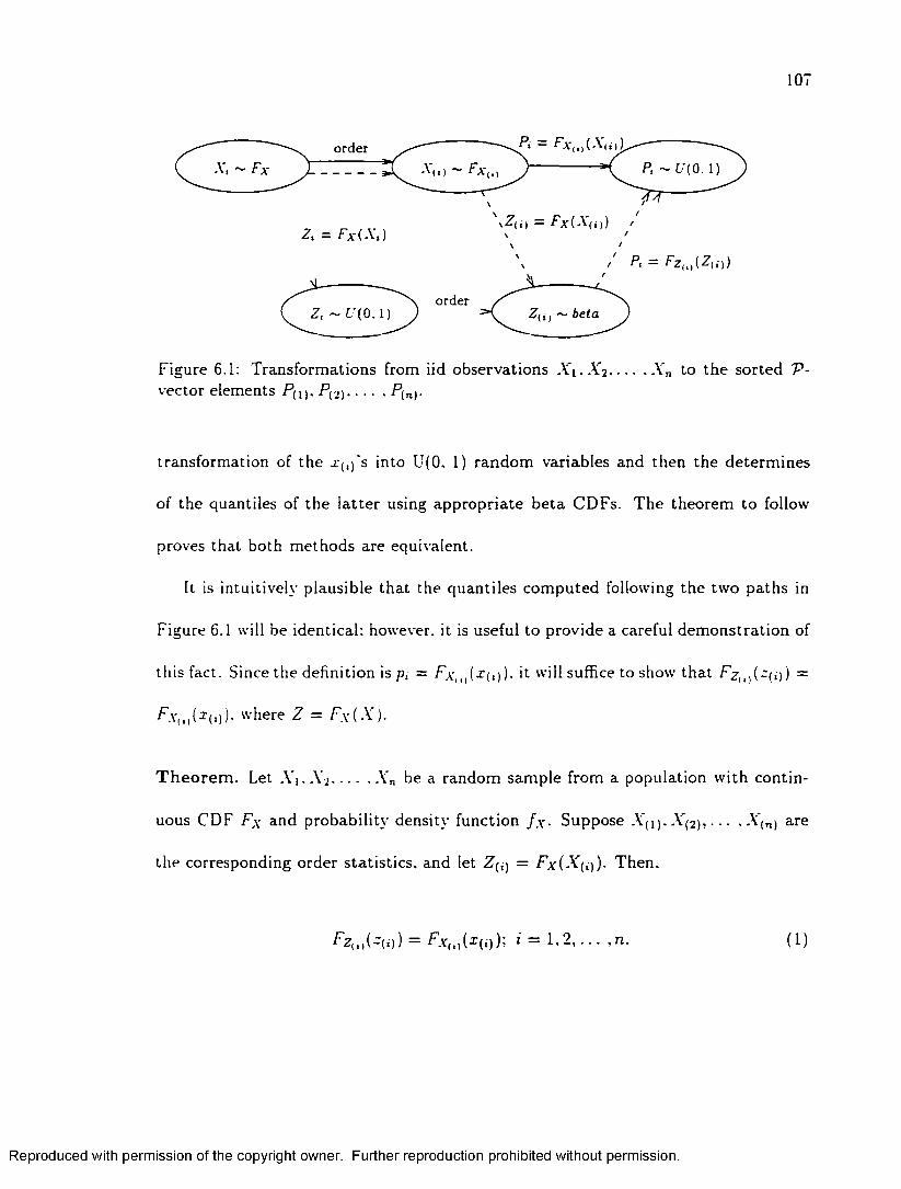
107

order

order

Figure 6.1: T ransfo rm ations from iid observations A 1 ..A 2 .......... A'„ to th e so rted V-vector elem ents P^). P^2)...........P{n)-

transform ation of th e X(,)'s in to U(0. 1) ran d o m variables and th en th e de te rm in es

of th e quantiles of th e la tte r using ap p ro p ria te b e ta C D Fs. T he theo rem to follow

proves th a t bo th m ethods are equivalent.

It is in tu itively p lausib le th a t the quan tiles com p u ted following th e tw o p a th s in

F igure 6.1 will be iden tical: however, it is useful to provide a careful d em o n stra tio n of

th is fact. Since th e defin ition is p, = F v Ml(x(,)). it will suffice to show th a t Fzu){~(i)) =

F.\U)(x {l)). w here Z = Fx (X ) .

T h e o r e m . Let A"i. X 2 V„ be a random sam ple from a popula tion w ith co n tin

uous CD F Fx and p ro b ab ility density function f x - Suppose A’(i).A '(2) , ..........\ ( n) are

th e corresponding o rder s ta tis tic s , and let Z(;j = F x (X ^ ) ) . T hen .

FZ{, ,(-(£)) = Fjr(l)( x (i)); i = 1 , 2 , . . . , n. (1)


108

P ro o f . B oth sides of E quation (1) will be reduced to equivalen t forms. For th e left-

hand side of E quation (1). no te th a t Z(,-) ~ beta(i.rc — i + 1) (B arr and Zehna, 19S3)

and th a t

,,(-(«■)) = FZ{j F x (x{t])) = FZ{t) o F x (x (i)).

T he C D F of a b e ta ( i .n — i + 1) random variable is defined by

Fz,jx) = k f : z - ' u - : r -d z .

nlwhere h = —-----— ----------— T hus th e com position above is given bv

(i — l)!(n — 0 ! 5

(*(.’)) = k r - l ( l - : ) n~'dz.Jo

. r F x ( i ( l ) )

° Fx

Now consider th e rig h t-h an d side of Equation (1). T he density of .V(l) is given by

/.v ,„ (x ) = k[Fx (x)]'~l [l - Fx (x)]n- ' f x (x)

(Larsen and M arx. 1986). so th e corresponding C D F is

FXit)( x (t]) = k r " [ F x { s ) ] - l [(l - Fx (s))]n~ ' f x (s)ds.J — o c

Make th e change o f variab le r = Fx {s) so th a t —oo < s < X(,j «=> 0 < c < Fx (x^))

109

and dz = f x ( s ) d s . T he right-hand side of E quation (1) is therefore given by

F.v,„ ( * < , ) ) = 1 - = -f*,., 0 ^ < * < 0 )

□

O ne could also develop the quantile p, following the lower path in F igure 6.1. T he

p a th ind icated in F igure 6.1 by the dashed line is generally preferred, since th e dis

trib u tio n s leading to th e p, elem ents are polynom ials. T he com putations needed for

the solid p a th are calculable, however they typ ically tak e a significantly longer tim e

to calcu la te . Also, th e C D F of X is typ ically m ore trac tab le than th e C D Fs of A'(,)'s.

6.4 G ood n ess-o f-fit te s t in g

In general, goodness-of-fit testing involves s ta tin g a null hypothesis. Ho : f x { x \ d ) =

/o (x :$o) a nd then assessing w hether there is sufficient evidence in a random sam ple

to reject Hq. Since th e 'P-vector was derived under Ho, one sees th a t its elem ents

provide a d irec t judgm en t of fit. Any p, too low or too high may be an ind ica tion of

a poor fit. It would be useful to form a single s ta tis tic based on th e p ,’s th a t ind ica ten n

good or bad fit. Som e obvious cand idate te s t s ta tis tic s are ^ |p, — 0.5 |. D p . - o -s)2t= l i= i

n iand 5 2 |p ( i) ------------ 1. These test sta tis tics, however, ap p ea r to suffer from low pow er,

.= i n + 1

based on a m odest set of sim ulations th a t were conducted . Instead , a varia tion of

th e reasoning th a t seem s im plicit in the developm ent of A nderson-D arling (A -D ) A 2

s ta tis tic was considered. C alculations are done according to the p robab ility in tegral

110

transform ation p resen ted in th e second form in S tephens (1986, p. 101). N ote th a t

the A -D .4 2 s ta tis tic is developed w ith th e Z(t) values which are dep ic ted in the lower-

right s ta te of F igure 6.1. Define a te st s ta tis tic in te rm s of a linear com bination of

the n a tu ra l logarithm s of p, and 1 — pt . This te s t s ta tis tic will be large w henever

one or m ore p ,'s is too close to 1 o r 0. Sort the elem ents of the "P-vector, so p(i) is

t U/t n rv» 1 1 nr t /-k f a1 *"V rvk n t o f f Un ' f l t /% »• f l> a 1 axvnn f F\ »* 4 U a »k llV J l i l U l l C J b WL b llW V .lC iU V .U b O O l b U C / ' W V .b V i ( U t U / ' ( n ) i 0 i a i g v . o b . 1 ^ / d l l l C L l iC I C 3 1

sta tis tic P3 by

Ps = - n - ~ X ][(2 n + 1 - 2i) ln(p(t)) + (2* - 1) ln( 1 - p(l,)]. (2)n

T he power of Ps was exam ined in a series of sim ulations. T he goodness-of-fit te s ts

based on P3 have pow er about th a t of A 2 in m ost cases, and b o th P3 and A 2 generally

dom inate th e K -S te s t, as s ta ted in D ’A gostino (1986, p. 110). for th e A -D te s t.

T here is a t least one case where P3 dom inates th e A -D test: the case of g uard ing

against an im proper variance p a ra m e te r under th e null and a lte rn a te hypotheses of

norm ality.

The test using P3 as a test s ta t is tic is significantly m ore powerful th a n bo th th e

K -S and A -D tests in th e following experim ent. T he power of th e th ree tests was

approx im ated , and a fourth test P* using p, in place o f p(,j in E quation (2), un d er

the following conditions. Let Ho '■ -V ~ N (0 ,1) and H a : X ~ iV(0,<72). R andom

sam ples were gen era ted of size 10 from N ( 0 , a 2) w here a vaxied from 0 . 1 ,0 . 2 , . . . . 3.0.

A plot of each te s t’s es tim ated pow er a t guard ing against changes in <r, based on 1000

I l l

replications of th e sim u la tion , is shown in Figure 6.2.

1-51 0

0.8

04

K-S

02

0.0

00 0.5 1.0 l i 10 15 30

Figure 6.2: E stim a ted pow er functions for testing H 0: X ~ N ( 0 .1) versus H .V ~ N(0.<r2) using K -S , A -D . and two s ta tis tic s based on th e P -v ec to r .

T hese power p lo ts show th a t as a becom es g rea te r th a n 1. b o th P, and P / have

significantly higher pow er th a n have A 2 and Dn. Also. P* sligh tly outperform s Ps for

a > 1. As a becom es less th a n 1, Ps clearly outperform s A 2 and D n . bu t P j has very

low power. T he s tro n g perform ance of Ps, four tim es th e pow er of A 2 a t a = 0.30,

for exam ple, causes us to con jectu re th a t th is is a s trong om nibus te st s ta tis tic for

guard ing against d e p a rtu re s from hypothesized variance for N(Q,cr2) populations.

T h e s tan d ard erro r of e s tim a te of a power value 1 — /? is less th a n \J (0.001)(/?)(1 — 4 ),

o r abou t 0.015 for ind iv id u a l values p lo tted in th e m id -heigh t range of F igure 6.2.

T hus th e im provem ent in power of Ps over A 2 is significant as ev iden t in F igure 6.2.

Since Ps seem s to provide protection in b o th directions of d e p a rtu re of a from 1. it

w arran ts one to investigate m ore fully its critica l poin ts. D ue to th e dependence of

the pi e lem ents, finding an analy tical expression for the d is tr ib u tio n of these s ta tis tic s

seems un tenab le: however, using sim ulation , approx im ated c ritica l points for the Ps

are shown in T ab le G.l. Note th a t th e critica l points of all s ta tis tic s are those of

th e fully specified null d istribu tion , case zero in D’A gostino 's te x t. T he sim ulation

for th is tab le relied on 10.000 itera tions of each sam ple size, so only two dig its are

significant. N ote th a t the d istribu tion of Ps seems to have a heavy right ta il, and as

n increases, the ta il becomes heavier. It is also in teresting to no te th a t for n < 25

the th ree critica l values increase alm ost exac tly linearly.

Table 6.1: E s tim a ted critical values for P3 a t various sam ple sizes and levels of significance.

n 0.90 0.95 0.992 4.9 6.1 8.93 7.6 9.1 13.44 10.1 12.1 17.05 12.6 15.3 21.56 15.1 1S.1 24.47 17.7 21.1 2S.28 20.4 23.9 32.09 22.7 26.8 36.510 24.9 29.4 39.511 27.9 32.2 43.712 30.0 35.2 48.015 37.5 44.0 59.620 50.7 58.7 81.125 63.2 76.2 116.530 80.0 107.1 218.440 445.0 576.5 776.850 1025.4 1108.8 1231.6

1 1 3

6.5 C on clusion

The purposes of th is chapter are two-fold. F irst, th e no tion of using the inform ation

contained in th e fit of order s ta tis tic s is presented, as represen ted in the P -v ecto r. as

a vehicle to define a new goodness-of-fit te st s ta tis tic Ps. T he perform ance of Ps w ith

sim ulation experim en ts was exam ined. F igure 6.2 shows convincing evidence th a t P,

is a powerful goodness-of-fit test a t least in some instances, so it is adm issible relative

to Dn and A 2. A secondary purpose is to show th a t th is procedure is p ractical

to carry o u t. now th a t com putational languages such as M aple are becom ing fully

developed. Indeed , th e code in M aple used to com pute th e critical values in Table

6.1 consists of abo u t one page. E m bedded in th a t code is th e ability to find the

n-fold vector of polynom ials represen ting the each of degree up to n . th a t

make up th e b e ta d is tribu ted CD Fs used to calculate th e P -v ec to r elem ents. T he

leverage in th e approach through th e Z(,-j is th a t M aple crea tes and stores the C D Fs.

not the p rogram m er. The sam e sim ulation in FO R T R A N or C' would require the

program m er to hard-code the n polynom ial CDFs for each value of sam ple size in

Table 6.1. and th en call a separate subrou tine to ca lcu la te th e test sta tistics. This

could be a significant program m ing task . T he M aple version requires none of th is,

since the C D Fs are in functional form and may be eva lua ted a t specific points. Not

only th a t, b u t for large n. in the case of n — 50 for exam ple, th e 50 CD Fs of the o rder

sta tistics m ay have extrem ely large in tegers for the coefficients of the term s, as well as

for their exponen ts. M aple is able to conduct the m a th em a tica l operations w ithou t


1 1 4

rep resen ting these constan ts as floating point approx im ations. T hus the precision

exceeds an im plem en tation in a high-level algorithm ic language. It is apparen t th a t

the adm issib ility of Ps suggests a ttra c tiv e procedures for o u tlie r detection and th a t

inferences w ith censored sam ples m ay also be defined in te rm s o f th e P -vecto r.


C hapter 7

O ther A pplications and E xam ples

7.1 In trod u ction

A key con trib u tio n of A PP L is th a t it provides a new way of viewing ex is tin g p ro b

lems and opens new avenues for th e ir solution. This chap te r provides exam ples w here

the problem -solving parad igm can sh ift due to the ab ility to find exact d is tr ib u tio n s

of random variables. T he six sections th a t follow highlight som e diverse a rea s of ap

p lication th a t can be addressed w ith A P P L . The chap ter s ta r ts w ith re la tiv e ly sim ple

exam ples involving the cen tra l lim it theorem (CLT). In these exam ples o n e will be

able to d e te rm in e th e erro r o f th e CLT approxim ations to d is trib u tio n s invo lv ing

sum s of independen t random variab les. T he second section con tains a d e m o n s tra

tion of how to use A PP L to g en era te m athem atically in tra c ta b le tab les, g ra p h s , and

charts , effectively reducing th e need for th e volumes con tain ing these e n titie s . T h e

th ird section contains a d em o n stra tio n of how com putation of exac t d is tr ib u tio n s can

115


1 1 6

enhance probab ilistic model design using re liab ility block diagram s. T he fourth sec

tion con ta in s a dem onstration of how the softw are allows for m odeling system s using

hazard functions. The fifth section provides a discussion on a sim ple m ethodology

by w hich A P P L furthers one's ab ility to identify ou tliers in sam ples. Finally, in th e

s ix th section , a discussion of some explorations for crea ting estim ation techn iques us

ing m ax im u m likelihood w ith o rder s ta tis tic d is tr ib u tio n s is given. T hese six exam ples

serve on ly to suggest the n a tu re of app lications of A PPL ; m any m ore app lica tions

exist.

7.2 E x a ctn ess in lieu o f CLT approxim ations

O ne use of th e CLT with iid sam ples is to fac ilita te inference about th e popu la tionn

m ean. T h e CLT implies th a t X = ^ A', is asym p to tica lly norm ally d is tr ib u ted w hen1 = 1

the A '.'s a re iid with finite mean and variance. A pplication of th e CLT becom es

res tric ted , however, w ith sm all sam ple sizes, w ith skewed da ta , or in th e presence of

ou tliers (M oore and M cCabe 1993. p. 510). In these cases, an a lte rn a tiv e m e th o d

is to d e te rm in e the exact d is tribu tion of X . O nce the d istribu tion X is found, one

can use it to m ake s ta tis tica l inferences about th e popula tion mean. A few exam ples

follow.

Let A" ~ e x p o n e n tia l 1). By th e CLT, the ap p ro x im ate d istribu tion of Y = X is

ap p ro x im ate ly N (l, ^ ) . For the case n = 3, one can com pute the exact d is tr ib u tio n

of Y w ith th e following com m ands:


11'

> X> n> Y> Y

= E x p o n e n t i a lR V ( l ) ;= 3;= SumIID(X, n ) ;= Transforra(Y, [ [x -> x / n ] , [0, i n f i n i t y ] ] ) ;

T he resulting PD F is f y { y ) = y y 2e-3y for y > 0 w hich is p redic tab ly non-norm al

in shape, as n is too low for the norm ality o f th e CLT to apply to such a skewed

underly ing d is tribu tion . O ne also notes th a t V has th e Erlang d is tribu tion . Now

consider the case n = 30, often considered a sufficiently large sam ple size for an

adequa te CLT approx im ation . Here a co m p u ta tio n of th e error associated w ith th e

approxim ation is provided. To obtain the P D F of X , one changes th e second line of

code to n := 30 ; and re-executes the M aple w orksheet. T he result is the following

Erlang PD F:

. , . 24631531333923339S437500000 29 _30uf v (u ) = -----------------------------------------------v eJ 10577732774609 y y > 0

Listed below are selected fractiles for bo th th e exact d is tribu tion of X and its CLT

approx im ation , the N (l. d istribu tion . For th e selected fractiles. the approxim a-

Table 7.1: F ractiles for exact and app ro x im ated distribu tions.

A pproach D istribu tionFractile

0.9 0.95 0.975 0.99ExactCLT

X 1.2401.234

1.3181.300

1.3881.358

1.4731.425

tion is only good to abou t one digit beyond th e decim al point. It is useful to no te

th a t the CLT approx im ation for critical values in confidence intervals for E ( X ) m ay

be in error; worse, they are not even on the conservative side. For exam ple, a 97.5%


118

u p p er confidence bound using th e CLT quan tile 1.357S4 actually provides only 96.6%

confidence [note P ( X < 1.35784) = 0.965975 is found in th e M aple w orksheet w ith

th e com m and CDF(Xbar, 1 .3 5 7 8 3 8 8 2 9 );] . N ote, th e add itional A P P L com m ands

to genera te the values in T ab le 7.1 are th e following:

> Z := N orm alR V (l, 1 / s q r t ( 3 0 ) ) ;> a lp h a := [ 0 .9 , 0 .9 5 , 0 .9 7 5 , 0 .9 9 ] ;> f o r i from 1 t o 4 do> IDF(Y, a l p h a [ i ] ) ;> IDFCZ, a l p h a [ i ] ) ;> od;

For a related ap p lica tio n , consider an old, app ro x im ate m eth o d of genera ting

random samples from th e s ta n d a rd norm al d is trib u tio n . It is well d o cu m en ted (P ark

and Leemis, 1997. for exam ple) th a t the following approach can be used to genera te

approx im ate ly s tan d ard norm al sam ples, w here th e U\'s are iid U(0. 1):

T he following com m ands d e te rm in e the exact d is trib u tio n of th is 12-fold convolution

and th e th ird and fourth m om ents of Z ’ and Z:

> U := UniformRV(0, 1 ) ;> U12 := SumIID(U, 12) ;> Z s t a r := Transform (U12, [ [ x -> x - 6 ] , [ - i n f i n i t y , i n f i n i t y ] ] ) ;> Z := NormalRV(0, 1 ) ;> skew := x -> x “ 3;> k u r t := x -> x “ 4;> e v a l f ( E x p e c t a t i o n R V ( Z s t a r , skew)) ;> e v a l f (E x p e c ta t io n R V ( Z , sk ew )) ;> e v a l f ( E x p e c t a t i o n R V ( Z s t a r , k u r t ) ) ;> e v a l f (E x p e c ta t io n R V ( Z , k u r t ) ) ;

119

T he d istribu tion of Z* is useful because, like th e s tan d ard norm al d is tr ib u tio n , its3

/ Z ' - E \ Z ' \ \\ )

m ean is zero, its variance is one, and its skew ness ( th ird m om ent. E

E [(Z*)3 ) is also zero. T he first difference is in th e fourth m om ent E [(Z *)4j which

equals 2.9 for Z ’ and 3.0 for a standard norm al random variable Z. A n o th e r m ore ob

vious difference betw een th e d istribu tions of Z and Z" is th a t Z has su p p o rt (—oc. oo)

w hile Z ’ has supp o rt ( —6 .6 ). T he d is tr ib u tio n of Z “ is th e following:

f z ' ( x ) = <

39916600

L£Lj20160 J

1

(6 + x) li165950373 3 2 6 4 0 0

1517

10060 X' — 24 6 _ 11737200 7200 X5 - 250657 3 _ 1 1 1 3 3 1 7 2

20160 1 6 0 4 6 0 X

67200 69472

________ -1 1 _ 47-26777 __________3 6 2 6 6 0 0 i 3 0 2400 *■ 3 0 2 4 0

11 9 _ 5 4 7 9 7 410060 '

— —— xa *+■665280 ^ 576 x ^, 9385 2 i I

^ 1728 X ^ 17280

7 , 631 61120 1440 x99121.10

1199 5 , 12199 38 0 0 £ “r 2 240 *

+ x nsrcn •**:25760 '3 8 5 3 311200 X + 11

10080_ 9 , 1009 4£ ^ 288 £ '

6 1297 o oo , uj o _166320 2016 X 560 X 72 x

1 4 3 .5 . 4 00 x 11

- 3 _ 1 119 21120 £ 3024

8 06465521

1 X11 _ x _ —LL- x* _ ^ r2 4 1 9 2 0 £ 5600 x 6 7 2 0 £ 504 x

166320

+

4 - — — x 4 *‘ 25211 11 X * + - ■ j*® + r *1680 x T 360 ^ 1200 x

583L121239 „ 4

11 563 x~3 3 6 0 x 3024 x

120960 6551

11

6 5 5 1 1

X +

23

11

1663200 "*■ 1440 360 0 X809

4320809

504 oX’ —

+ _L_ x 6 _ _ 2 3 _ 6 _ ^ _1663300 T 1440 360 0 x 4320 x

144001

14400

X1 0 -

X10 +6 6400

16 6400

x“ + ^x -< r 11 + ^ x 4

65521 I i _ 8 _166320 ^ 252 -LL. x r A— — x 6 —1680 x ^ 360 x

563 - X ^ — x -1200 x 3 3 6 0 x 3024 x

120960 ^ 6 1 2 9 7 25

11 50400 X — 10080 X* +

n.2

25504

.1020

8 . _33_ 7 _ 1_3 6 , M 3 5 iL ' x 7 0 x i i n n x '166320 2016 ^ 560 ^ 72 * ^ 400

1 r 10 , 1 -1 1 , 781_ , I I . 9 _ 239 48064 x ^ 2 4 1 9 2 0 x T 5600 x ^ 6 7 2 0 x 504 x *

8 9 4 7 2 7 , _7__ 8 _ 99 7 , 631 6 _ 1199 5 _ 12199665280 576 1120 ^ 1440 x 8 0 0 22

3 _1120 x 3024 x

1619

2 2409385 „2 i 1.

* i —+ JUWW —_

T726 17280.10

i x l 1 -7 2 5760 x3 8 5 3 3

1°1- r* -20160

167200 x 10 +

11200 1 6 595037 3 3 2 6 4 0 0

1

X — 1110060 X + 1009 4

2 66 X ’

1120 '3 6 2 6 6 0 0

-2_ x ~ -| SL260 T 1 0 0

. 1 1

517- 7* ' _ 2477 ,10080 * 7200 x

r 11 + 4726777 , 302400 x 1 :

T6 —27 5 _ 243 _50 X 35 2

6 , 11737 5 , 25065' 7200 "*

11 ,

3 _ 111331720160 1 6 0 4 6 0

3 9 9 1 6 6 0 0 '_ 2 9 ^ 6 I_

175 x 20160 Xs +

3 0 2 4 03 . 466 2

‘r 35 x 1 7 496 , 6 1 4 1925 35 X

5 4 7 9 7 410060 ’

1604600 '

.1 0

—6 < x < —5

—5 < x < —4

—4 < x < —3

- 3 < x < - 2

- 2 < x < - 1

- 1 < x < 0

0 < x < 1

1 < x < 2

2 < x < 3

3 < x < 4

4 < x < 5

5 < x < 6

In the overlaid M aple plots of th e s ta n d a rd norm al PD F and f z - { x ) show n in

F igure 7.1, it is ap p aren t th a t this ap p ro x im ate d is trib u tio n fits th e s ta n d a rd norm al

d is tr ib u tio n in the PD F very nicely except a ro u n d x = 0 [where f z { 0) = = 0.399

120

and f z - { 0) = fgfoVod — 0-394] and. of course, in th e tails, since th e app ro x im ate

d is trib u tio n only has support on (—6. 6). To o b ta in overlaid p lo ts of th ese two

d is trib u tio n s , one invokes the P l o t D i s t com m and. F irs t one creates a p lo t of Z~ and

stores it as P l o t l . Next, one creates a plot of th e s tan d ard norm al d is tr ib u tio n and

stores it as P lo t2 . Finally, used the p l o t s [ d i s p l a y ] com m and to com bine th e two

plots. T his is sum m arized in the com m ands:

> P l o t l := P l o t D i s t ( Z s t a r , - 6 , 6 ) ;> P l o t 2 := Plo tDis t(NormalRV(0, 1 ) , - 6 , 6 ) ;> p l o t s [ d i s p l a y ] ( P l o t l , P l o t 2 , s c a l i n g = u n c o n s t r a i n e d ) ;

xl

F igure 7.1: Overlaid plots of f z - ( x ) an d th e s tan d ard norm al P D F .


121

7.3 A m a th em atica l resource gen erator

A PP L is also able to g en era te tab les, graphs, and charts. T h e te rm resource refers to

tab les, graphs, and charts, to include such item s as m eans, critica l points, variances,

and so on. A PPL can be invoked to reduce the need for such tables. A dditionally ,

since these com putations can be produced au tom atically , program s can be designed

to produce needed values in real tim e, as opposed to being restric ted to know ing in

advance which elem ent of w hich tab le will be needed for p rogram execution. T h ere

are many references for c ritica l tab les for com mon d is trib u tio n s th a t softw are such as

th is (and o thers) effectively replace. H ighlighted, however, will be two recent books.

CRC Handbook of Tables f o r Order Statistics from Inverse Gaussian Distributions

with Applications (B alak rishnan and C hen, 1997) and C R C Handbook of Tables for

the Use o f Order Statistics in Estimation (H arter and B alakrishnan , 1996). T hese

books were selected because o f th e relatively com plex n a tu re of the inform ation they

present. Also, they were chosen to highlight th a t even as la te as 1997, the scientific

com m unity had to rely on tab les and charts for a significant am ount of p robab ilis tic

inform ation.

F irst is a com parison of B alak rishnan and C hen 's C R C Handbook of Tables for

Order Statistics from Inverse Gaussian Distributions with Applications w ith A P P L ’s

capabilities. This book begins w ith 39 pages of theory and references to the inverse

G aussian (IG ) d istribu tion a n d its o rder s tatistics. T hen th e book has 645 pages of

P D F plots, expected value tab les , covariance tables, es tim a tio n tables, and so fo rth .


A P P L is able to c rea te a n u m b er of these figures and tab les , and in som e cases goes

beyond those presented in th e te x t. Page 50. for exam ple, shows th e N ( 0 ,1) a n d th e

s tan d ard ized IG(O.S) P D F s overlaid in a single plot. T h e s tandard ized IG d is tr ib u tio n

the P D F of Z (which is listed as equation (2.14) on page 7 of the te x t) is as follows:

Then the two plots may be overlaid as follows:

> X := NormalRV(0, 1) ;> k := 0 . 8 ;> Z := [ [ z -> 1 / s q r t ( 2 * P i ) * (3 / (3 + k * z ) ) (3 / 2) *

e x p ( - 3 * z “ 2 / ( 2 * ( 3 + k * z ) ) ) ] , [-3 / k , i n f i n i t y ] ,[ ‘Cont i n u o u s ' , ' PDFf ] ] ;

> P l o t l := P l o t D i s t ( X , - 4 , 4 ) ;> P l o t 2 := P l o t D i s t ( Z , - 4 , 4 ) ;> p l o t s [ d i s p l a y ] ( { P l o t 1, P l o t 2 > , s c a l i n g = u n c o n s t r a i n e d ) ;

T he M aple-produced plot is found in Figure 7.2. B alak rishnan and C hen use such

plots to show how the two d is tr ib u tio n separate as k increases from zero. For p lo ttin g

th e IG P D F , one is not lim ited to th e s tandard ized version of the d is tr ib u tio n . O ne

could plot any IG P D F . C D F , H F. and so on. For exam ple , th e com m and

> P lo t D i s t ( H F ( I n v e r s e G a u s s i a n R V ( l , 0 . 5 ) ) , 0, 3 ) ;

will genera te a plot of th e IG (1. 0.5) hazard function. C learly, one is n o t lim ited

to ju s t P D F plots in A P P L , nor is one lim ited to p lo ts of only s ta n d a rd iz e d IG

d is trib u tio n s .

is defined as follows. Let Y ~ IG(A.<5). Let a = \J8ZI A (th e s tan d a rd d ev ia tio n of

Y) . Define Z = (V — 8 ) /a as th e s tan d ard IG d is trib u tio n , and let k = 8 / A. T hen

3=2 /(6-f-2Jt=) 3— - < : < o c .

AT

Figure 7.2: O verla id plots of the s tan d a rd norm al and s tan d ard ized IG(O.S) d is tr ib u tions.

A nother recen t resource. CRC Handbook of Tables for the L'se o f Order Statistics

in Estimation (H a rte r and B alakrishnan, 1996), also gives ex tensive ch a rts for various

app lications of o rder sta tistics. A ppendix C of this book, covering pages 326-530.

lists tab les of various m eans, variances, and covariances of o rd e r s ta tis tic s from m any

com m on d is trib u tio n s . For exam ple. T able C l . l gives m eans of o rd e r s ta tis tic s for

the N (0 ,1) d is tr ib u tio n . Table C2.1 for th e e x p o n e n tia l 1) o rd e r s ta tis tic s , and so on.

A PP L can rep lica te such tables. For in stance , to produce the m ean of th e n = 8, r = 6

order s ta tis tic from the W eibull(l, 0.5) d is trib u tio n , use th e com m ands:

> X := WeibullRVCl, 0 . 5 ) ;> X86 := O r d e r S t a t ( X , 8, 6 ) ;


> MeanRV(X86);

which re tu rn e d the value 1.760598073. com pared to 1.76060 on page 392 of H arte r

and B alakrishnan (1996).

U nlike H arte r 's te x t, th e softw are can go beyond co m p u tin g m eans of o rder s ta tis

tics. In th e following exam ple (con tinu ing the code from th e th ree lines of code above),

one can, for exam ple, com pute th e 98th percentile o f th e sam e W eibull d is trib u tio n

and give th e probab ility of exceeding 1.92:

> IDF(X86, 0 . 9 8 ) ;> SF(X86 , 1 .9 2 ) ;

T he values re tu rned are 6.480288415 and 0.0473928543. respectively. F urtherm ore , we

are not lim ited to the relatively few base d istrib u tio n s th a t H arte r and B alak rishnan

present in A ppendix C. bu t can en te r any W eibull p a ra m e te r values.

T here is no im plication th a t these, or any of th e vast resource collections, are

archaic. A ctually, w hat is envisioned is the need of th is softw are to augm ent the

inform ation presented in te x ts such as these. Foreseen is a sh ifting away from looking

up values in table: instead, one will encode th e c rea tion of necessary values d irec tly

into program s. The first 208 pages of H arter's te x t, for exam ple , still review theory

behind th e creation and use of o rder s ta tis tics. A P P L adds to th e resource base th a t

books such as these provide.


1 2 5

7.4 P rob ab ilistic m od el design: re liab ility b lock

diagram s

T h e analysis of reliability block diagram s (R B D ) in reliab ility engineering can be

fac ilita ted by use of A PP L . A program called S H A R P E (Sym bolic H ierarchical A u

to m ated R eliab ility /P erfo rm ance Evaluator, p resen ted in S ahner and Trivedi. 1993)

uses M athem atica to m odel reliab ility block d iagram s and o th e r types of system s. In

th e ir artic le . Sahner and Trivedi show how S H A R P E is capab le of providing system

reliab ilities. However, according to Trivedi (1997), inp u t d is tr ib u tio n s are lim ited to

exponen tia l d istribu tions and “exponential polynom ials w hich are equivalen t to Cox

d is tribu tions." A PPL can conduct sim ilar com puta tions and is not lim ited to such

d is tribu tions. A d em onstra tion is provided by dup lica ting T rived i's exam ple, and

then showing possible extensions. This is not m eant to be a d irec t com parison of

S H A R P E and A PPL . as th e two software packages have com plete ly different goals.

T h e tw o softwares m erely in tersect to some degree, as th is RBD exam ple shows.

In Sahner and Trivedi (1993). a com puter system consists of two processors and

th ree m em ory units. T he com p u ter is designed to o p era te w ith as few as one processor

and one m em ory unit. T hus a RBD to represent the system would be as shown in

F igure 7.3. in which two paralle l processors are in series w ith th ree parallel m em ory

un its. All com ponents are independent and have exponen tia lly d is tr ib u ted tim es to

failure.

T h e C D F of of X sys. th e tim e to failure of th e system , can be determ ined w ith


1 2 6

PROC

PROC

MEMORY

MEMORY

MEMORY

F igure 7.3: RBD of a co m p u ter system w ith tw o processors and th ree m em ory un its.

th e following com m ands in A PPL :

> Xp := E xponen t ia lR V (0 .00139);> Xm := E xponen t ia lR V (0 .00764);> Xsys := MinimumRV(MaximumRV(Xp, Xp) , MajcimumRV(MaximumRV(Xm, Xm) , Xm));> Xsys := CDF(Xsys) ;

T h e result is th e following C D F

f ( x ' ) = [ _ g e ~ 0 .0 0 9 0 3 r _j_ g e ~ 0 .0 1 6 6 7 x _ .}g - 0 .0 2 4 3 1 x 2 g - 0 - 0 1 0 4 2 x _ g £ - 0 .0 1 8 0 6 x e ~ 0 .0 2 5 7 x

w here x > 0. W hile th is C D F is different from th a t in T rived i’s a rtic le , in a subsequen t

personal com m unication (Trivedi 1997), T rivedi agrees th is expression is th e correct

C D F ; th e one in the a r tic le being in error.

T h e areas for im provem ent of problem solving by A P P L are m any. F irs t, w ith

A P P L one can m odel th e tim e to failure of th e ind iv idual com ponents w ith d is trib u -


1 2 7

tions o ther th an th e exponential. Second, one can ana lyze the system by looking a t

th e functioned form of th e C D F (as in S H A R P E ), b u t also graphically, by p lo ttin g

th e d is tribu tion . T rivedi m entions th a t a p lo ttin g function is curren tly in b e ta te stin g

for SH A R PE (T rivedi. 1997). One can also d e te rm in e and plot the SF. H F. C H F .

and PD F of th e system . O ne can sum Xsys an d Xsys to find th e d istribu tion of the

life tim e of two such system s in a passive s tan d b y configuration using SumRV. Fractiles

of th e d is tribu tions can be produced. O ne can cond u c t “w hat-if" analysis by varying

th e num ber of processors and m em ory un its in th e sy stem to see th e overall effect on

th e m ean system lifetim e. O ne can run a re liab ility life te st to see if observed failure

tim es are adequa te ly fit by th is model, using th e goodness-of-fit techniques ou tlin ed

in C h ap te r 6.

7.5 M o d elin g w ith hazard fu n ctio n s

T h e capab ilities of A P P L allow a shift in th e p a rad ig m of param eterized m odel design

in new ways. In som e situ a tio n s , it m ay be easy to im agine th e reliability of a sy stem

in te rm s of in s tan tan eo u s ra te of failure, i.e.. th e haza rd function . R eliability tex ts

o ften classify lifetim e d is tribu tions into distribution classes th a t are nam ed a fte r th e

sh ap e of the hazard function. Leemis (1995, C h a p te r 3), am ong others, defines m any

of th ese classes, to include the increasing failure ra te (IF R ), th e decreasing fa ilu re

ra te (D FR ), and th e b a th tu b (B T) shaped haza rd function .

O ne possible use for A P P L is to m odel system s using a hypothesized shape of a


12S

h azard function. For exam ple, should a system be hypothesized to have a b a th tu b

shaped HF. th e re a re only a few common d is trib u tio n s w ith H Fs w ith such a shape.

Leemis (1995, p. 100) lists only two of 16 com m on re liab ility d is trib u tio n s as having a

B T -shaped HF. In stead of being lim ited to these d is tr ib u tio n s , one m ay hypothesize a

fam ily of d is tribu tions w ith B T-shaped HFs. For exam ple, a second-order polynom ial

H F of the form a(x — b)2 will have th e B T shape as long as a > 0 and 6 > 0. It is

easy to verify these polynom ials satisfy th e requ irem en ts for a H F. as listed in Leemis

(1995. p. 50):

f h(i)dt = oc and h(t) > 0 for all t > 0 .Jo

H ere is an exam ple of using A PPL to m odel w ith hypothesized H Fs. Let a sam ple

of failure tim es be [1. 11. 14. 16. 17]. A ssum ing it is hypothesized th a t th e system

should be fit by the q u ad ra tic BT-shaped H F d is trib u tio n , one should fit these d a ta

to th e unspecified d is tr ib u tio n as follows.

> a ssu m e (a > 0 ) ;> assu m e(b > 0 ) ;> T := [ [ t -> a * ( t - b) " 2 ] , [0 , i n f i n i t y ] , [ 'C o n t i n u o u s ' , 'H F '] ] ;> P D F (T );

T h e last com m and re tu rn s th e general form of th e P D F having th e assum ed HF:

f T(t) = a( t2 - 2tb + b2) e~ta{t2- 3tb+3b2)/3 t > 0 .

O ne can find th e values of a and b th a t m axim ize likelihood as follows:

> sam p le := [ l , 11 , 14 , 16, 1 7 ];


12 9

> h a t := MLE(T, sample , [a , b ] ) ;> e v a l f ( h a t ) ;

T he results are: a = 0.0037937. 6 = 5.93512. T he plot of the SF for T overla id on the

em pirical SF is shown in Figure 7.4.

Sir)1.0

0.6

0. 4

0.2

o.o

5 150 10

Figure 7.4: The SF of th e hypothesized B T -shaped hazard function fit to th e sam ple [1. 11. 14. 16. 17] overlaid on the em pirica l SF.

For another exam ple of m odeling in te rm s of hazard functions, let us hypo thesize

th a t risk to a system is seasonal. Such is th e case in m any applications such as s tru c

tu res a t risk to occurrences of category five hurricanes. A periodic haza rd function

m ight be modeled in such a case. Suppose one hypothesizes a family of period ic HF


130

d is trib u tio n s having HFs of the form

hj ( t ) = a + b s in (c f) . t > 0; a > |6|, and a . i . c G 3?.

O nce again, these functions satisfy th e req u irem en ts of HFs. T h e p a ra m e te r a rep

resen ts a m easure of th e long-term co n stan t risk associated w ith T. In o th e r words,

increased values of a correnspond to a h igher likelihood of chance failures. T he pa

ram eters b and c con tro l th e am p litu d e an d period of the H F. m odeling th e severity

and length of th e cyclic stresses.

In the ir artic le . Lee. W ilson, and C raw ford (1991) m odeled seasonal ocean storm

d a ta in term s of a nonhom ogeneous Poisson process w ith in ten s ity function of the

form

A( < ) = e » + - t > 0 : a . 7 . u / , o G 3?

w here th e exponen tia tion is used to assu re th a t A(t) > 0 for all t. T h ere are two

differences betw een the N H P P m odel o f Lee, W ilson, and C raw ford (1991) and m od

eling w ith a seasonal hazard function. F irs t, th e in tensity function m e th o d models

m u ltip le occurrences of seasonal events w hile th e hazard function m e th o d m odels a

single occurrence. Second, th e in ten sity function m ethod assum es th a t th e process

has independent increm ents, am ong o th e r assum ptions (see Ross, 1993, p. 236, for

all assum ptions). Such assum ptions a re not necessary w ith h aza rd function models.

O ne can in s ta n tia te the unspecified d is tr ib u tio n w ith the following com m and

> T := [ [ t -> a + b * s i n ( c * t ) ] , [ 0 , i n f i n i t y ] , [ 'C o n t i n u o u s ' , 'H F ' ] ] ;

131

and th e PD F m ay be found with the com m and PDF(X) T he unspecified P D F of

th is fam ily of d is tr ib u tio n s w ith a periodic hazard function is

f T (t) = (a + b s in ( c t ) ) e - {atc- cosict)b+b}/c t > 0 .

L etting the p a ram eters take on values of a = 1, b = 0.5 and c = 10. O ne gets the

P D F (using th e P l o t D i s t com m and) p lo tted in F igure 7.5. a peculiarly m ulti-m odal

d is tribu tion th a t decreases exponentially over tim e.

| l\! 11i i i

■i ■ n ' 'I '

F igure 7.5: T he P D F of th e d is trib u tio n having periodic hazard function h x w ith param eters a = 1. b = 0.5 and c = 10.


7.6 O utlier d etectio n

T h e theory and p rac tice of identifying ou tliers in a d a ta set is ano ther con tribu tion

provided by A P P L . T he lite ra tu re contains am ple m ethods for identifying outliers in

sam ples re la ted to a norm al d is tribu tion . R egarding detection of outliers. D 'A gostino

(1986. p. 497) w rites “We shall discuss here only th e underly ing assum ption of norm al

ity since th e re is very little theory for any o th e r case.” S arhan and G reenberg (1962.

p. 302) and D avid (19S1) propose a num ber of te st s ta tis tic s based on s tandard ized

o rder s ta tis tic s of norm ally d is tribu ted d a ta . T hey provide charts of accep tance and

rejection regions in lieu of p-values. For instance, in th e fully specified case w here p

and a are knowm, S arhan and G reenberg propose th e te s t s ta tis tic (A jn) — p)/cr for

testing for ex trem e observations in norm al sam ples. As has been discussed in C hap ter

6. the d is trib u tio n s of o rder sta tistics can be used to identify outliers in d a ta sets.

A PPL m ay co n trib u te to the ou tlier de tection problem in a t least th ree ways:

1. T here is no need to standard ize th e te s t s ta tis tic , since th e d is trib u tio n of the

r th o rder s ta tis tic m ay be found w ith th e procedure O r d e rS ta t .

2. O ne need no longer rely on charts of rejection regions, since once th e d istribu tion

of th e r th o rder s ta tis tic is known, one can calcu la te p-values.

3. M ost im portan tly , one is not lim ited to th e assum ption of norm ality . A PPL

fac ilita tes finding th e d istribu tion of th e r th o rder s ta tis tic of a w ide range of

d istrib u tio n s .


133

Here are a few exam ples. In th e sam ple 1. 2. 3. 4. 5. 10. it is possib le th a t

the last elem ent in th e sam ple is an o u tlie r. Assum ing th a t th e popu la tio n has a

m ean of 3. one could find the o rder s ta t is tic probability P { X ^ ) > 10) for sam ples of

size 6 from various underly ing d is trib u tio n s . Let us consider th e following possib le

population d is tr ib u tio n s , each w ith m ean of 3 (approxim ately 3 for th e W eibull case):

W eibull(0.295. 2). e x p o n e n tia l 1 /3). N (3. 2). and N(3, 4). T h e upper ta il p ro b ab ility

P{X(6) > 10) gives us the significance level against th e null hypothesis th a t A’(6)

cam e from this underly ing d is tribu tion . T h e four p robab ilities can be found w ith th e

following com m ands:

> XI := WeibullRV( 0 .2 9 5 , 2 . 0 ) ;> X2 := E xpo n en t ia lR V ( l / 3 ) ;> X3 := NormalRV(3 , 2 ) ;> X4 := NormalRV(3 , 4 ) ;> O r d e r S t a t ( X I , 6 , 6 ) ;> SF (" , 10);> e v a l f ( S F ( O r d e r S t a t ( X 2 , 6, 6 ) , 1 0 ) ) ;> e v a l f ( S F ( O r d e r S t a t ( X 3 , 6, 6 ) , 1 0 ) ) ;> e v a l f ( S F ( 0 r d e r S t a t ( X 4 , 6, 6 ) , 1 0 ) ) ;

The resu lts are show n in Table 7.2. An in te rp re ta tio n is th a t for n = 6 th e value 10

T able 7.2: P { A'(6) > 10) for n = 6 for several popu la tion d istrib u tio n s .

D istribu tion

oAl7?

aT

W eibull(0 .295,2) e x p o n e n tia l( l/3 )

N (3 ,2) N (3 .4 )

0.00099660.19583850.00139500.2175316

is an o u tlie r w ith resp ec t to th e N(3, 2) d is trib u tio n a t th e 0.0014 level of significance

and to th e W eibull(0.295, 2) popula tion d is trib u tio n a t th e 0.001 level of significance.


1 3 4

It is no t a sign ificant o u tlie r to the o the r two p o p u la tio n d istribu tions. C learly one is

not lim ited to m ax im u m values of a sam ple, one could also consider any of th e o rder

s ta tis tic s (as o u tlin ed in th e C hapter 6. using the ’P -v ec to r) . N ote, these four u p p er

ta il p robab ilities a re th e 6 th elem ent of the four V - vecto rs. Also note th e lack of p a ra l

lelism in th e com m ands. O ne would expect th e com m and e v a l f (SF ( O r d e r S ta t (XI ,

6 , 6 ) , 10) ) w ould have produced th e ap p ro p ria te p ro b ab ility for th e W eibull d is tr i

bution. However. M ap le locked up w ith this em bedding . By separa ting th e com m and

into two p a rts . M aple com puted th e p robab ility co rrec tly and quickly.

An ex tension to th is detection exam ple is found in th e last two popu la tion d is tr i

butions, th e norm al d is trib u tio n s w ith cr equal to 2 an d 4. O ne sets a specified level

of significance, say a = 0.05, and solves for th e value o f a th a t will show a m axim um

value of 10 to be an o u tlie r for th e norm al family o f d is trib u tio n s . T here a re two

d irections to th is so lu tion . F irst one m ight be te m p te d to conduct a b inary search

on the in terval 2 < o < 4 to approxim ate s to a ce rta in degree of accuracy. T he

following code will accom plish th a t approx im ation a n d will derive a — = 2.9297.

a lp h a := 0 .0 5 ; s i g o l d := 4; signew := 2; fo u n d := f a l s e ; w h i l e ( f o u n d = f a l s e ) do

X := NormalRV(3, s ignew ) ;s i g n i f i c a n c e := e v a l f ( S F ( 0 r d e r S t a t ( X , 6, 6 ) , 1 0 ) ) ; d e l t a := a b s ( s i g n i f i c a n c e - a l p h a ) ; i f ( d e l t a < 0 .0 0 0 0 1 ) th e n

found = t r u e ;p r i n t ( s i g m a i s n o w , s i g o l d ) ; b re a k ;

e l s ei f ( s i g n i f i c a n c e < a lp h a ) t h e n

temp := s ig n ew ;s ignew := s ignew + abs (s ignew - s i g o l d ) / 2; s i g o l d := temp;

1 3 5

p r in t (n e w s ig m a , s ignew ) ; e l s e

temp := signew;signew := signew - a b s ( s ig n e w - s i g o l d ) / 2;s i g o l d := temp;p r in t ( n e w s ig m a , s i g n e w ) ;

f i ;f i ;

od;

A second approach is to rely on th e exactness of d is tribu tions th a t A PPL provides.

In effect w hat is desired is a so lu tion to the following. L etting X ~ N(3. a), find a

such th a t

P ( X (6) < 10) = 0.95.

One can find th a t exactly by m a n ip u la tin g th e CD F list-of-lists rep resen ta tion of

A(6) in the following way. T he first elem ent of the first list will contain the C D F ,

so it is set equal to 0.95 and solved for c. T he following code produces the solu tion

a S 2.933571640.

> X := NormalRV(3, s ) ;> X6 := O r d e r S t a t ( X , 6, 6 ) ;> X6 := CDF(X6);> f s o l v e ( X 6 [ l ] [1 ] (1 0 ) = 0 . 9 5 , s = 2 . . 4 ) ;

T he first line of code sets the sem i-specified norm al d is trib u tio n as the popu la tion

d is trib u tio n for A’. T he second line determ ines th e P D F of A(6). T he th ird line

converts th e P D F of A'(6) to a C D F. T h e last line isolates th e first elem ent of the first

list of X6 w hich is th e CD F function of th e independent variable x and th e unknow n

p aram eter a. T h e en try (10) provides th e independent variable a value of 10. T h en

the f s o lv e com m and solves for th e unknow n p aram eter s which represents a.

1 3 6

T he sam e ty p e of de term ina tion could be m ade for any of th e d is trib u tio n fam ilies.

O ne can likewise, for exam ple, d e te rm in e th e value of fi th a t re jects 10 as an ou tlier.

In effect, one is ab le to establish a d is tr ib u tio n 's to lerance in terval for a p a ram eter,

given a specific m in im um or m axim um d a ta value. T hus th e detec tion of ou tliers is

relative to an assum ed underlying d is trib u tio n , and one can p a rtitio n the p aram ete r

space of underly ing d istribu tions in te rm s of ou tlier consistency.

7.7 M axim u m lik elih ood o f order sta tistic s d istr i

b u tion s

An idea is presen ted in this section th a t has some in tu itive appeal towards im proving

estim ation of param eters . Borrow ing from the idea of es tim atin g param eters via

m axim um likelihood, and also suggesting th a t order s ta tis tic s m ight be helpful in

es tim ating p aram eters , the usual form of the likelihood function.

L i ( x .d ) =i=i

(where x = (x t . x 2l • • • . J n )). is rep laced w ith a form involving th e PD Fs of the o rder

sta tistics:

£ a( x .0 ) = f [ / j r ,:= 1

T he second m ethod is referred to as m ax im um likelihood estim ation w ith o rder s ta t is

tics (M LEO S). N ote th a t L\ is th e jo in t d is tribu tion of iid random variables. T h e


137

function Lo does not lend itself to such a d irect rep resen ta tio n , as o rder s ta tis tic s a re

not indep en d en t.

T h is approach to estim ation borrow s from the in tu itio n associa ted w ith trad itio n a l

m axim um likelihood estim ation . In his Figure 7.7. Leem is (1995. p. 172-173) gives

a graph ical in te rp re ta tio n of th e M LE m ethod. Leemis suggests th e goal of M LE is

to find th e p a ram e te r 9 th a t "m axim izes the p roduct of th e density values a t th e

d a ta p o in ts .” S ince in MLE one seeks a value of 6 th a t m axim izes th e p roduct of th e

density values from the PD F. it was wondered w hat w ould happen if the p ro d u c t of

the density values of the n order s ta tis tic s was m axim ized . M axim izing the p ro d u c t

of th e "hum p -sh ap ed ” order s ta tis tic P D F s evaluated a t th e ir respective ordered d a ta

values is g raph ically depicted as finding a 9 value th a t m axim izes th e product of th e

lengths of th e vertical lines in F igure 7.6 (th e lines from th e o rdered d a ta poin ts to

the ir o rdered density values). A good fit places each of th e d a ta values near th e

center of th e n hum ps of the n P D F s. M LEOS will find a A value th a t m axim izes th e

p roducts of th e respective density values. Note the x m arks on th e horizontal axis

correspond to th e sam ple [0.2. 0.4. 0.9. 1.5].

P a ra m e te r es tim ates were com puted from various popu la tio n d istrib u tio n s from

sim ulation using bo th MLE and M LEO S. T he em pirica l m ean square errors (M SE)

of th e two es tim a tio n techniques w ere com pared. Also com pared were estim ates for

A from th e exponen tia l d is trib u tio n , fi and a from th e norm al d is tr ib u tio n , and 9

from th e (* (0 ,0 ) d istribu tion . O f all these population d is tr ib u tio n s , only th e la st

case, e s tim a tin g 9 from the uniform d is tribu tion , resu lted in a decrease in M SE of th e


138

f(2)<*(2))2.5 2.5

2.0 2.0

1.5

1.0

0.5

0.0 0.0

0 3 0 34 i 4

2.5

2.0

1.5

1.0

0.5

0.0

30 -> 4

2.5

2.0

1.5

1.0

0.5

0.0

F igure 7.6: T he P D F s of the four o rder s ta tis tic s from an exponential d is tr ib u tio n .

es tim ato r. S ince som e ML estim ato rs are also m in im um variance unbiased e s tim a to rs

(M V U E ). it not feasible for M LEOS to dom inate M LE w ith respect to M SE. T his

is th e case for e s tim a tin g A for th e exponential d is tr ib u tio n and fj for th e norm al

d is tr ib u tio n (K endall and S tu a rt, 1963). However, th e p a ram e te r <r from th e norm al

d is tr ib u tio n is not a M V U E (K endall and S tu a r t, 1963, p. 10) and th e M L E for

0 in th e uniform d is tr ib u tio n is biased (Larsen and M arx , 1986, p. 244). For th e

uniform d is trib u tio n , th e reason th a t th e M LEOS e s tim a to r dom inated th e M LE

139

estim ato r is easy to see. Each MLE estim ate of 6 is th e m axim um of th e sam ple.

The M LEOS estim ato r for 6 is e ither the m axim um d a ta value, or th e solution to

aL*d6 ^ = O' abou t 32% of th e samples, th e solution to this equation was greater

than th e m axim um of th e sam ple. The sim ulation com parisons of th e MLE and

MLEOS estim ators were designed as follows: set the sam ple size to 25. and the

num ber of replications to 1000. For the sim ulation it was assum ed th a t 0 = 1 . and

population variates from th e U(0. 1) d is trib u tio n were generated . T he M aple code

for this sim ulation is included in A ppendix H. Also included is th e perform ance of

the unbiased estim ato r for 0. which is m ax{A ’i, A V . . . . A^}. T he results are

given in Table 7.3. T he M LEO S estim ato r had less bias and a lower M SE than th e

Table 7.3: The MSEs of th e M LE and MLEOS and adjusted-for-bias M LE techniques of param eter estim ation .

Technique Average E stim ate MSE of E stim ates

MLE 0.9615 0.002768MLEOS 0.9720 0.002020

MLE w ith unbiased factor 0.9999 0.0013SS

MLE estim ato r. As could be expected , however, th e ML estim ato r w ith th e unbiasing

factor. !i d. m ax{A 'i . A t An }, dom inates on bo th m easures.


Chapter 8

C onclusion and Further Work

This d issertation presen ts work on a proposed probability softw are language. We have

dem onstrated some areas of app licab ility and contributions to the applied com m unity

provided by this softw are. As it exists. A P P L is a viable language th a t dem onstrab ly

con tribu tes to the app lied com m unity. A t its core, it is a tool to produce th e d is tri

bution functions of random variables. O nce these d istribu tion functions are known,

then all the typical p robab ility work th a t is done with d is trib u tio n s is possible, i.e..

significance levels, c ritica l poin ts, expec ta tions, plots, and so on. T here is a veritab le

lifetim e's am ount of research th a t rem ains w ith APPL. T he areas for fu rth er work fall

into two categories, im provem ents to A P P L itself, and fu rth er areas of app lica tion .

The language itse lf has po ten tia l for fu rth e r im provem ent. So far it is re s tric ted to

univariate , continuous d is tribu tions. M ultivariate considerations could follow. Also,

m ore procedures could be devised to include areas of probability such as condition ing ,

Bayesian analysis, tim e series analysis, po in t processes, and o thers . A dditionally ,

140


141

the softw are could encom pass d iscrete d istribu tions, as well as m ixed d isc re te and

continuous d is trib u tio n s .

A pplication a rea s are endless for A PPL . A num ber were presented here, b u t th e re

are m any m ore areas th a t could benefit from such softw are. These areas inc lude

p aram eter e s tim a tio n and goodness-of-fit testing in censored sam ples, finding th e d is

trib u tio n of th e to ta l-tim e-o n -te s t in a life-testing env ironm ent (surprising sim ila rities

exist here w ith th e difficult in tegration of th e K -S C D F ), and renewal theory, to nam e

a few. As A P P L becom es m ore exposed, countless o th e r areas will em erge.

Finally, th e re is an o th e r inherent con tribu tion in th a t th e softw are has been kep t

ex trem ely general on purpose. Consider the crea to rs of th e spreadsheet. T hey had th e

insight to m ake th e app lica tion general enough th a t it solved the ir cu rren t p ro b lem

yet could be app lied to m any larger problem s. Decades la te r no researcher, business

office, or s tu d e n t 's room is com plete w ithout a s ta te -o f-th e-a rt spreadsheet a t th e ir

disposal. T his so ftw are research has m ain tained th is sam e sp irit of g enera lity for

sim ilar reasons. For exam ple, by allowing for param eterized , piecewise d is tr ib u tio n

in the "list-of-lists” fo rm at, nearly every continuous, un ivaria te d is tr ib u tio n can be

represented by A P P L . T hus the software can be of use to the reliab ility eng ineer

concerned w ith a ran d o m variable having suppo rt (O .oo), as well as th e th e o ris t who

is in terested in th e o rd er s ta tis tic s from populations having segm ented d is tr ib u tio n s

with supp o rt in th e negative range. W hile probably no t as com m on or w idely needed

as th e sp read sh ee t, th e au th o r foresees the possib ility th a t eventually no p ro b a b il is ts

resources will be co m ple te w ithout a sym bolic p robab ility package w ith p rocedu res


1 4 2

such as these. T h u s, th e generality of A P P L is yet ano ther co n trib u tio n because it

allows for yet unseen con tribu tions by those in te res ted in expanding the probabilistic

world via an a u to m a te d , program m ing env ironm en t.


A ppendix A

The A rctangent Survival

D istribution

A .l In trod u ction

This appendix con tains som e early work on crea ting new d is trib u tio n s of random

variables based on th e SF-like qualities of th e a rc tangen t function. T h e work in tro

duced the au thor to th e need for software th a t could assist in p robab ility calculations,

p lots, and o ther functions. P resented here is th e developm ent of a tw o-param eter

survival d istribu tion th a t has an upside-down b a th tu b (U B T . or hum ped-shaped)

hazard function. T h is d is trib u tio n provides b iosta tis tic ians, re liab ility engineers, and

o th e r s ta tistic ians w ith a second tw o-param eter U B T model whose closed-form su r

vivor function sim plifies th e analysis of right-censored d a ta sets. M axim um likelihood

estim ators of the p a ram eters a re found using num erical m ethods. A pprox im ate con-

143


1 4 4

fidence in tervals can be determ ined by using th e observed inform ation m atrix or th e

likelihood ra tio s ta tis tic . Exam ples are given in which the a rc tan g en t d is trib u tio n is

a reasonable a lte rn a tiv e to o ther com mon lifetim e distributions.

P a ram e tric lifetim e d istribu tions have been used in reliability for m odeling the

tim e to failure of com ponents and system s. A lthough em phasis has trad itio n a lly been

placed on m odels w here th e hazard function has a ba th tu b shape, app lications have

been found w here an upside-dow n b a th tu b (U B T ). or hum p-shaped hazard function

is the ap p ro p ria te m odel. Kececioglu (1991, p. 425) lists transisto rs, m etals su b jec ted

to a lte rn a tin g stress levels, insulation deg rada tion , m echanical devices sub jected to

wear, and bearings as po ten tia l UBT applications. Chhikara and Folks (1989, p. 156)

s ta te th a t "W hen early occurrences such as p roduct failures or repairs are dom inan t

in a lifetim e d is trib u tio n , its failure ra te is expected to be non-m onotonic, first in

creasing and la te r decreasing" and cite a irbo rne com m unication transceivers (p. 5.

139-140) as an app lica tion . Lee (1992. p. 12) fu rther supports the valid ity of a U BT

risk m odel in describ ing pa tien ts w ith tubercu losis who have risks th a t ''increase in i

tially. th en decrease afte r trea tm en t." To fu rth e r sub stan tia te th e usefulness of th e

UBT m odel. B arr (1994) opines th a t the U B T risk function would ap p ly in m odeling

the p robab ility of a soldier becom ing a casualty as a result of a rtille ry fire. In th is

exam ple, casu a lty risk s ta r ts ou t low as the fire is initially inaccurate , increases as th e

shooter hones in on th e ta rg e t, and then decreases as the rem aining soldiers are able to

"dig in” for p ro tec tion . A lthough reliability engineers generally have an abundance

of tw o-param eter survival d is tribu tions to choose from, relatively few have a U B T


145

hazard function . T h e com m oniy-used UBT d is trib u tio n s are th e inverse G aussian ,

log norm al, an d log logistic d is tribu tions. Of these, only th e log logistic d is trib u tio n

has a closed-form surv ival function. This d is tribu tion is m ost o ften used in b iosta tis-

tical app lica tions, w hereas the inverse Gaussian and log norm al are typ ica lly used in

reliability.

T he a rc tan g en t d is tr ib u tio n developed here gives a survival d is tr ib u tio n w ith a

UBT hazard function and closed-form survivor function, a useful fea tu re in th e anal

ysis of a righ t-censored d a ta set. A dditionally, the surv ivor function can be inverted

in closed-form . w hich enables synchronization and m ono ton ic ity in v a ria te genera

tion. U nlike m ost surv ival d is trib u tio n s , the a rc tan g en t d is tr ib u tio n ’s developm ent

uses trigonom etric functions. We present the a rc tan g en t d is tr ib u tio n 's developm ent,

probabilistic p ro p ertie s , and s ta tis tic a l inference. P a ram e te r e s tim a tio n for com plete

and right-censored d a ta sets is found by m axim um likelihood. F inally , th ree exam ples

illu stra te s itu a tio n s w hen the d is trib u tio n is a dem onstrab ly reasonab le a lte rn a tiv e

to o ther surv ival d is tr ib u tio n s .

A. 2 D ev e lo p m en t

T he a rc tan g en t function , when negated and shifted vertically , resem bles a surv ivor

function. F u rth e r, by sh ifting th e function so th a t it crosses th e v ertica l axis a t 1 and

then asy m p to tica lly decreases to 0, one obtains a flexible su rv ivor function . A dding


1 4 6

a phase shift param eter 0 and a positive scaling param eter a yields the function

r 1g ( t ) = — a rc tan [a(f — o)j + — — 00 < t < 00.

which is a decreasing function w ith a range of (0. tt). Finally, since ^ (0 ) = a rc ta n (a o )+

the ap p ro p ria te way to ad ju st th is function so th a t it assum es th e value 1 when

t = 0 is to d iv ide g(t) by ^ (0 ), y ield ing the survivor function for th e ran d o m lifetim e

T

— a rc ta n [a (f — 0)1 + £

* ( < | - a r c t a l ( U + f ' ~ °'

Since th e a rc tan g en t is an odd function, the form of th e surv ivor function th a t will

be used here is

a rc ta n [a (o — <)] + ? arctan(a<z>) + j

where q > 0 and —oc < 0 < cc. T h is survivor function satisfies th e th ree existence

conditions: 5 (0 ) = 1. lim 5 (f ) = 0. and S( t ) is nonincreasing. F u rtherm ore , thet — OC

d is tr ib u tio n 's p robab ility density function and hazard function are

f T { t ) = — S T ( t ) =a

a rc ta n (a 5 ) + f 1 + oc2 { t — <Z>)2t > 0. ( 2 )

h T { t )frit)Sr{ t )

a

arctan[a(<z> — t ) } + | 1 + a 2(t — <f>)2t > 0. (3)

This arctangen t d istribution is equivalent to a Cauchy d istribu tion truncated on

147

th e left a t t = 0. Thus th e param eter a is sim ilar to a scale p a ram e te r and the

p a ra m e te r 0 is sim ilar to a phase shift or location param eter. F igu re A .l shows three

d ifferent P D F s of the a rc tan g en t d is tribu tion . N otice th a t as 0 becom es negative, the

tin0 .08

a = 0 .1 5 0 = - 10.0

0 .0 6

a = 0 .1 5 <(> = 20.0

0 .04

0.02

a = 0 .0 4 0 = 5 0 .0

0.0I

200 40 60 80 100

F igure A .l: Exam ples of the arc tan g en t probab ility density function.

d is tr ib u tio n changes from a bell-shaped d is trib u tio n to a d is trib u tio n w ith a m ode of

0. Also no tice th a t th e p aram ete r a controls the “peakedness” of th e d is tribu tion :

th e d ispersion of the d is tr ib u tio n is a decreasing function of a.

In itia lly the nam e “A rctangen t D is trib u tio n ,” was chosen because of th e sim i

la rities th a t the arc tangen t function has w ith a generic survivor function. T h e re

la tionsh ip to the Cauchy d is trib u tio n was noticed la ter. T he C D F of th e C auchy

d is tr ib u tio n is also a sh ifted and scaled a rc tan g en t function.

L4S

A .3 P rob ab ilistic properties

T h e arc tan g en t d is trib u tio n has several useful p robab ilistic p roperties th a t m ake it

a v iable d is tribu tion for lifetim e d a ta analysis. Specifically, it enjoys closed-form

su rv ivo r and hazard functions, unlike m ost d is tr ib u tio n s in the U B T class. T he

closed-form survivor function simplifies p aram ete r es tim ation for censored d a ta sets

and allows for variate genera tion via inversion. T h e probabilistic p ro p erties include:

• T he d is tribu tion is in th e UBT class w hen a d > c and is in th e decreasing

failure ra te (D FR ) class when ad < c w here

1 -f 2 carc tan (c ) + cir = 0.

found by sim plifying h'T(0) = 0. Using num erical m ethods, c ss —0.42S9S.

• T he m ode of th e d is trib u tio n is £mode = o. V d > 0. For th e case w here th e

probab ility density function is m onotonically decreasing, £mode = 0< V o < 0.

• T he pth fractile of th e d is tribu tion is

1tp = o -1— tan

Q

which yields a m edian of

10.5 — <P 4— tan a

— — — arctan(a<£) .

i l / A

— — (1 — p) ( a rc tan (ac)) 4- — (4)

1 4 9

T his closed-form expression for the fractiles will be useful in determ in ing in i

tia l e s tim ates for th e num erical m ethods required to d e te rm in e th e m axim um

likelihood es tim ates.

• V ariates can be genera ted via inversion by

1T *— 0 -1— tan a

-j- — (1 — i')(^ arctan(a<z>) + —

w here U is un iform ly d is trib u ted betw een 0 and 1 .

• T he cond itional surv ivor function is given by

ST(t)^T]T>a(l) =

5 r ( a )arctan[a(<z> — <)] + t arctan[a(<z> — a)] + -|

arctan[a(c> — a) — (f — a )] + t arctan[a(c> — a)] + f

a rc ta n [a ( 7 - y)] + f a rc ta n fa '/j + |

for y > 0 . w hich is again an a rc tan g en t d is tr ib u tio n w ith th e sam e a as the

u ncond itional d is trib u tio n and w here 7 — 0 — a and y = t — a.

• T he lim iting d is tr ib u tio n as a —+ 0 0 is a degenerate d is tr ib u tio n a t <t>.

• T h e a rc tan g en t d is trib u tio n is re la ted to th e C auchy d is tr ib u tio n . Specifically,

a C auchy d is trib u tio n tru n ca ted on th e left a t zero will y ie ld th e a rc tangen t

d is tr ib u tio n . N ot surprisingly, th e m ean and h ig her-o rder m om ents of the dis-

1 5 0

tr ib u tio n are undefined. T h is poses a challenge when discussing m ean tim e to

failure (M T T F ) of com ponents. Since th e mean is undefined, cen tra l tendencies

of th e d is trib u tio n could be d iscussed in term s of its m ode and m edian. T h e dis

advan tage of th is lim itation is th a t p ractitioners are generally m ore com fortab le

w ith the m ean as the p rim ary m easure of central tendency.

• T he a rc tan g en t d is trib u tio n has a heavy right ta il which makes it useful for

evaluating an item th a t fails w ith less risk once it has survived to a ce rta in

tim e threshold . C ertain b io s ta tis tic a l d a ta sets ind icate such heavy righ t ta ils

in cancer d a ta . T he a rc ta n g e n t d is trib u tio n is capable of m odeling lifetim e

d is trib u tio n s w ith a heavier ta il th a n th e log norm al or log logistic. An exam ple

is provided w here th e d is tr ib u tio n m odels the survival tim e of ra ts given a cancer

accelera ting drug, where th e re is a heavy right tail. C om peting risks m odels are

also useful in m odeling heavy right ta ils.

A .4 S ta tis tica l in feren ce

S ta tis tic a l inference of the a rc tan g en t d is trib u tio n for com plete and right-censored

d a ta sets is straightforw ard . A com parison w ith o ther d is trib u tio n s , including o th e r

com m only used U BT d is tribu tions is p resen ted in this section. T he a rc tan g en t d is tr i

b u tio n requires num erical m ethods to d e te rm in e the m axim um likelihood es tim a to rs

of its param eters , which is typ ical of m ost tw o-param eter lifetim e m odels. F irs t,

s ta tis tic a l inference procedures for uncensored d a ta are p resen ted using a re liab ility


exam ple. Second, inferences are illu s tra ted w ith censored d a ta using a b iosta tistica l

d a ta set. F inally , a b iosta tistical exam ple th a t illustrates th e heavy righ t-hand tail

of th e d is tr ib u tio n is presented.

For the uncensored case, let t \ . t 2 tn be th e failure tim es. T he likelihood

function is

L(a. 0) = I I = 1 1Q

i=l i=l arctan(a<£) + | 1 -I- a 2(t l - o)2

T he first p a rtia l derivatives of log L ( a , d) w ith respect to the two p a ram ete rs yield

d log L ( a .d ) da

—no

1 -(- (ad )2 § + arctan(a<p) i=i 1 + a 2(ti — o)2

and

d log L(a . o) do

— na

1 -I- (ao)2 f -f a r c ta n (a o )+ E

t=i

2 a 2(t t - o )

1 + a 2(t{ — d )2( 6 )

E quating (5) and (6) to zero does not yield closed-form solutions for th e m axim um

likelihood es tim a to rs q and ©. For th e num erical m ethods to be effective in finding

a and o it is necessary to have app rop ria te in itia l estim ates of the p aram eters . Since

th e m ean and h igher o rder m om ents are undefined, one m ust rely on a “m ethod of

fractiles” . as opposed to th e m ethod of m om ents, to find in itia l e s tim ates d 0 and do-

T his entails an in itia l system of two equations based on th e pth frac tile of th e the

1 5 2

d is trib u tio n , where the fractiles are chosen based on th e observed lifetim e data .

To illu s tra te the app licab ility of th e a rc tan g en t d is tr ib u tio n , consider Lieblein and

Zelen’s (1956) d a ta set of n = 23 ball bearing failure tim es (each m easurem ent in 106

revolutions):

17.88 28.92 33.00 41.52 42.12 45.60 48.48

51.84 51.96 54.12 55.56 67.80 68.64 68.64

6S.8S 84.12 93.12 9S.64 105.12 105.84 127.92

128.04 173.40

A lthough it 's an old d a ta set, this is th e first exam ple because C row der e t al. (1991,

p. 63) con jectu red th a t th e U BT shaped d is trib u tio n s m ay fit th e ball bearing d a ta

b e tte r th a n th e IFR d istribu tions, based on th e values of th e log likelihood function

at the m axim um likelihood estim ators.

Using the "m ethod of fractiles'1 to find in itia l p a ram ete r e s tim a te s for the p aram

eters. no te from the em pirical survivor function for th e d a ta (F ig u re A .2) th a t tim e

42.12 corresponds to the 4L • 100 = 22.7th percen tile of th e d is tr ib u tio n and th a t tim e

105.12 corresponds to the • 100 = 82.6th percen tile of th e d is tr ib u tio n . Thus using

(4), in itia l estim ates for th e MLEs are found by solving

42.12 = © + — tanQ

105.12 = <p + — tanQ

f - ( i - ( a r c ta n ( a 0 ) +

^ “ ( i “ ^ | ) ( a r c t a n ( a 0 ) +

1 5 3

S(t)

n s

Weibull0.6

0.4

Arctangent0.2

0.0

100 150500

F igure A .2: E m pirical, fitted a rc tan g en t, a n d fitted W eibull su rv ivor functions for the ball bearing lifetim es.

for q and o. This system yields our in itia l estim ates of th e p a ram ete rs as follows:

q 0 = 0.04102 and Oq = 57.96. Using these values as in itia l e s tim a tes , one m ay now

solve equations (5) and (6) num erically y ield ing d = 0.04238 and © = 58.OS. Taking

second p a rtia l derivatives of th e log likelihood function and ev a lua ting a t the MLEs

yields th e 2 x 2 observed in fo rm ation m a trix (see Cox and O akes, 1984)

/ =

/ \ 5989 1.305

1.305 0.021

In v ertin g th e m a trix and tak ing th e square roo ts of the d iagonal e lem en ts gives asym p


1 5 4

to tically valid 95% approx im ate confidence intervals for a and o:

0.01727 < a < 0.06753

44.46 < d> < 71.70.

Figure A .2 gives a graphical com parison of the arctangen t fit versus the W eibull fit

of the em pirica l d a ta . O ne can see th e fits are virtually iden tica l in the early stages,

then th e a rc tan g en t fits m ore cioselv th a n does the W eibull in th e center. In th e

right ta il, th e W eibull fits closer, due to th e arctangent d is tr ib u tio n 's p ropensity for

a heavy ta il. F inally , one can com pare th e arctangen t d is tr ib u tio n 's m odel adequacy

w ith th a t of o th e r popular tw o-param eter lifetim e d istribu tions. T he K olm ogorov-

Sm irnov (K -S ) goodness-of-fit s ta tis tic for th e arctangent d is tr ib u tio n is Dn = 0.093.

Table A .l gives D n values for som e p opu la r d istribu tions fitted to the ball bearing

d a ta evaluated a t th e m axim um likelihood estim ators of th e ir param eters . [C hhikara

and Folks (19S9. p. 74) fit the inverse G aussian d istribu tion to th is d a ta set.] T h e K-S

s ta tis tic is one m easure to gauge quality o f fit. Table A .l ind icates th a t the lower K -S

Table A .l: K olm ogorov-Sm irnov G oodness-of-fit S tatistics for th e Ball B earing D ata .

D istribu tion D 2 3

E xponentialW eibullG am m aInverse G aussian A rctangen t Log norm al

0.3010.1520.1230.0990.0930.090

sta tis tic values are associated w ith th e th ree U BT d istribu tions, th e inverse G aussian .

155

a rc tan g en t, and log norm al, add ing fu rther credibility to C row der’s con jectu re th a t

U B T m odels seem to fit th is d a ta set b e tte r than those w ith increasing failure ra te s

(i.e., th e W eibull and gam m a d is tribu tions). Using a K -S s ta tis tic w ith e s tim a te d

p a ram eters is problem atic. T herefore , one uses this s ta tis tic not for a form al te s t,

bu t to fu rth e r th e conjecture th a t U B T d istribu tions fit th is d a ta set be tte r.

Now consider s ta tis tica l inference for a censored d a ta . T he arc tangen t d is tr i

bu tio n 's closed-form survivor function yields a closed-form likelihood function, thus

sim plifying th e analysis of right-censored data . T he only o th e r U B T d is trib u tio n w ith

this p ro p e rty is the log logistic d is trib u tio n . T he s ta tis tic a l m ethods are s im ila r to

those of th e uncensored case; however, th e num erical m ethods are a bit m ore ted ious.

An analysis follows for G ehan’s (1965) test d a ta of rem ission tim es from th e d ru g

6-.VIP w hen used on n = 21 leukem ia patien ts of which th e re were r = 9 observed

rem issions and 12 individuals who w ere random ly right censored. L etting an a s te risk

deno te a right-censored observation, th e remission tim es in weeks are:

6 6 6 6* 7 9* 10

10* 11* 13 16 17* 19* 20*

22 23 25* 32* 32* 34* 35*

To fit th is d a ta to th e a rc tan g en t d istribu tion , let £1? £2 , • • • • tn be th e rem ission

tim es and c i, c2, . . . . cn be the associated censoring tim es. O ur m axim um likelihood


1 5 6

es tim a tio n is now based on th e likelihood function

L(a,<f>) = S{ci,a,<f>)te c >ec

= 11rt

«€£.' a r c ta n (a o ) -f | 1 + a 2[t{ — d>)2n«ec

arctan(a(fi> — c,-)) 4- f arctan(a<!>) + %

w here U and C are th e sets of indices of uncensored and censored observations,

respectively . T he log likelihood function is

log Z ,(a .d ) = r l o g a — r log7T

arctan(a<p) + — - Y . + q2 (^ - ‘p)2]ieu

+ Y lo g [2 a rc tan [a (^ — c,)] + t ] — (n — r) log[2 arctan(ad>) + 7r]. ■ ec

A "m ethod of fractiles" in itia l estim ate for th e p a ram ete rs yields do = 0.0562 and

0O = 9.5S. Now one takes th e two partia l derivatives of log L w ith respec t to a and

o. se ts them equal to zero, and com putes d = 0.0455 and o — 11.2. T h is exam ple

illu s tra te s th e m ethodology used to fit th e a rc tan g en t d is trib u tio n to censored d a ta

sets.

A th ird exam ple illu s tra te s the usefulness of th e d is tr ib u tio n 's heavy righ t tail.

Cox and Snell (1981. p. 169) present d a ta on th e life span of ra ts who have been

given a cancer accelera to r. T he following com plete d a ta se t gives th e n u m b er of days

th e ra ts survived:

37 38 42 43 43 43 43 43 48 49 51 51 55 57 59 62 66 69 86 177

T h e arc tangen t M LE estim ates for th is d a ta set are a = 0.127 and <p = 48.0: the

resu lting arc tangen t d is trib u tio n is p lo tte d against th e em pirical su rv ivor function in

F igure A .3. Note how th e heavy rig h t ta il of the a rc tangen t d is tr ib u tio n m odels the

S(t)

0.6

0.4

0.2

0.0

50 100 1500

Figure A .3: T he a rc tan g en t d is tr ib u tio n fit to the ra t cancer d a ta .

heavy right tail of the ra t lifetim es. T h e ra t w ith survival tim e 177 is d riv in g th e fit.

T h u s , for d a ta sets w ith heavy ta ils such as this one, th e p rac titio n e r m ay m ake use

of th e arc tangen t d is trib u tio n 's p ro p en sity for a heavy righ t ta il.

158

A . 5 C onclusion

T h e arc tangen t d is tr ib u tio n is a tw o-param eter lifetim e d istribu tion in th e U B T class

w ith closed-form surv ivor function. It gives re liab ility engineers, b iosta tis tic ians , and

o th e rs ano ther tool in th e com plex task of s ta tis tic a l modeling. A lthough a UBT

m odel has a sm aller num ber of applications th a n does the IFR or b a th tu b -sh ap ed

m odels, there are enough references in th e lite ra tu re to indicate a need for more

d istrib u tio n s in th is class. T his appendix gives th e U B T model a second d is trib u tio n

th a t enjoys a closed-form surv ivor function and has been dem onstra ted to adequa te ly

describe well-known d a ta sets.


A p pend ix B

C ontinuous D istributions

T h e continuous d is tr ib u tio n s given in Table B .l are availab le when loading the file

c o n t d i s t .map. T he ta b le contains the function nam e used to define a random vari

able, th e P D F or C D F . th e support, and the p a ram eter nam es, and param ete r re

stric tions. O riginal references to the more obscure d is tr ib u tio n s are given in Leemis

(1995). Note th a t th e IDBRV is entered as a C D F in stead of a PD F in Table B .l.

M aple is able to d ifferen tia te the CD F into a PD F . but no t ab le to reverse th is opera

tion. C onverting from a P D F to a CD F for this d is tr ib u tio n resu lts in an unevaluated

in teg ral, which considerably slows com putations. R andom variables in A PP L defined

in th is fashion are in th e usual list-of-lists d a ta s tru c tu re , and the M aple assum e

function is used to re s tr ic t th e values of unspecified p a ram ete rs .

159


160

Table B .l: C ontinuous d is tribu tions of ran d o m variab les available in A PPL .

D istr ib u t io n n a m e P D F or C D F j S u p p o r t P a ra m ete r S p ace

E r la n g R V ( ) / A- ( x ) = X( Xx) n~ l e ' ^ / ( n - 1)! x > 0 0 < A < oo, integer nE x p o n e n t i a l R V ( ) f x ( x ) = x > 0 A > 0

Exponent ialPoserRV ( ) / A- ( x ) = e 1 _ ' ix eXz‘ Xk x k~ 1 r > 0 A > 0 : k > 0GammaRV( ) f x (x) = A ( A x ) * - 1e - A r/ r ( K ) x > 0 A > 0; k > 0

GeneralizedParetoRV() f x ( x ) = ( 7 + j £ y ) ( i + x / « x > 06 > 0 .7 > 0 . k > —67

G o m p e r tz R V ( ) f x (x) = 6Kt e - ttK*~l ) / 'a* K x > 0 6 > 0 : k > 1

ID B R V ( ) Fx (x) = l - d + K x r i ^ e - * * 3' 2 x > 0 7 , 6, k all > 0InTerseGauss ianRV() f x i x ) = \ / A / ( 2 Tx3 )e _A<r-,i)3 |2 ''3rl x > 0 A > 0. n > 0

L o g H o rm a lR V ( ) f . . ( r \ — _ l _ e - i lo g r -# i )J/ ( 2o J )JA V ' V2rxa x > 0 —00 0

M ak eh am R V Q f x ( x ) = (7 + 6 K r ) e - ’ r - 4('cX- I » /lo« 'c x > 0 7 , 6 > 0. «: > 1M u th R V O f x ( x ) = (e*x - l K+KX+ l l K x > 0 0 < K < 1

N o rm a lR V Q f x ( x ) = e - , z - » f l ° 3/ j 2 z < r 2 —oo < r < oc — OO < (1 < OO. O’ > 0P a r e to R V C ) f X ( x ) = k \ k / x k+1

( 2(r —a l

f x ( x ) = \ {b- j L mr; a)

x > A A > 0

T r i a n g u l a r R V ( )a < x < m m < x < 6

-0 0 f (6 —a )( b—m )

U n i lo r m R V O f x ( x ) = 1 / ( 6 - a ) a < x 0 A > 0. K > 0

A ppendix C

A lgorithm for 6 x 6 C onversions

T able C .l shows th e m a them atica l conversions of th e functional form s of random

variable d is tribu tions. T he tab le can be viewed as a from -to m a trix in th a t the

colum ns represent th e procedure nam e an d th e rows represent th e prior form of the

d is trib u tio n . Thus, if X is cu rren tly in C D F form , th e call to X := PDF(X) will convert

to th e C D F form v ia th e conversion listed in th e PDF colum n on th e CDF row.

Table C .l: T he conversions of continuous ran d o m variable d is tr ib u tio n forms.Procedure call w ith argument X

PriorForm PDFCI) CDFCX) SF(X) HFCI) CHF(X) IDF(X)

PD F Retum (X) fJ — OC

J n t ) d t

/ ( * >

J f i t ) d t - I n J f ( t ) d t F - ‘ (x)

CDF F '(x ) Retum(X) 1 - F (x ) F ' ( x )1 - F i x ) — In [l — F(x)] F - « ( x )

SF - S ' ( r ) 1 - S (x ) R e tu m (I) - S ' d )i ' l r l

— In [S(x)] F ~ H x )

HF - f h( t ) d th( x ) e

- f h( t ) d t1 - e

- f k ( t ) d te J — o o

R etu m (I) fJ — OO

F - ‘(x)

CHF / / ' ( x ) e - H (x» 1 - e - « > x > e - « ( x ) H ' ( x ) R etum (I) F ~ ‘ (x)

IDF F '(x ) F (x ) 1 - F ( x )1 — r < x )

— In [1 — F(r)] Retum (X )

161

1 6 2

Note th a t th e conversions to and from th e ID F require each functional form to be

converted to a C D F first, as tha t form is the necessary form for inversion. T hus F ~ l{x)

appreas in th e PDF, IDF(X) entry of T able C .l ra th e r than the m ore com plicated

f f ( t ) dtJ —OO


A ppendix D

A lgorithm s for Various Procedures

D .l A lg o r ith m for VerifyPDF

Procedure VerifyPDF verifies th e area under a P D F is one.

In p u t: A list-of-Iists rep resen ted random variable X w ith n segm ents.

Output: "True" or "F alse” depending if the area is equal to one.

.V «- PDF(X) area <— 0 for i 1 to n

area <— area + fx? '+l Xi , i ( x)dx if (area > 0.9999999 an d area < 1.0000001)

RETU RN (True) else

RETU R N (False)

163

1 6 4

D .2 A lgorith m for Expect a t ionRV

P rocedure E x p ec t a t ionRV (X, g ) finds the expected value of a function of a random

variable, i.e.. £[<7 (x)].

In p u t: A list-of-lists rep resen ted random variable X w ith n segm ents and a function

g(x).

O u tp u t: T he expected value of th e function.

.V «- PDF(X) expval <— 0 for i <— 1 to n

expval expval + /{■ .Yi,,(x) ■ g( x ) dxR E T U R N (expval)

165

D .3 A lgorith m for OrderStat

P rocedure O r d e r S ta t (X, n , r ) de term ines the PD F for the r th o rd e r s ta tis tic from

a sam ple size n sam pled random ly from a population w ith th e sam e d is trib u tio n as

the random variable A*.

In p u t: A list-of-lists rep resen ted random variable X w ith m segm ents and the integers

n and r .

O u tp u t: T he P D F of the o rder s ta t is tic A'(r ) in the list-of-lists fo rm at.

f X « - PDF(X)F A « - CDF(X) for i «— 1 to m

A-(r,,.,(</) - f iz if tn -* ' F X u ( y ) r~l • (1 - F X i , (y) )n- r • f * i A y )R E T U R N (A (r»)

166

D .4 A lgorith m for ProdllD

Procedure P ro d IID (X , n) determ ines the P D F for th e p roduct of n iid random vari

ables A".

In p u t: A list-of-lists represented random variab le X and the in teger n > I.

O u tpu t: T he P D F of Y = X n in the list-of-lists fo rm at.

A' «- PDF(X)Y «- ProductRV(X.X) for i <— 3 to n

Y <— ProductR V (A \ Y)RETU RN (V)

167

D .5 A lgorith m for SumRV

P rocedure SumRV(X, Y) determ ines th e PD F for th e sum of the independen t random

variables X and Y .

In p u t: Independen t random variables X and Y in th e list-of-lists form at.

O u tp u t: T h e PD F of V = A' -I- Y in the list-of-lists fo rm at.

IF <— ex [using Transform]Z <— eY [using Transform]V <— ln(VF • V) [using ProductRV and Transform]R E T U R N (F )

16S

D .6 A lgorith m for SumllD

P roced u re SumllD determ ines th e P D F for th e sum of n iid random variables ATi. X 2 A"„.

each having the sam e d is trib u tio n as X .

I n p u t : A list-of-lists rep resen ted random variable X w ith and th e in teger n > 1.

O u tp u t: T he P D F of }* = A’, in the list-of-lists fo rm at.

A — PDF(A)V <- SumRV(A. A ) for i <— 3 to n

Y <- SumRV(A, Y )R E T U R N (V)

169

D .7 A lgorith m for MininnimRV

P ro ced u re MinimumRV determ ines the P D F for th e m in im um of two independen t ra n

dom variables.

I n p u t : Two list-of-lists represented random variab les X and Y .

O utpu t: The P D F of V = m in{A '. V’} in th e list-of-lists form at.

f X — PDF(A) f Y « - PDF( Y) f V 2 - f X 2 U /V 2highest <— m in {m ax { /A '2} . m ax {/V 2}} [D elete elem ents above lower su p p o rt max] stoppoint <— ||/V 2|| [where || • || denotes card inality ]for i <— 1 to stoppoint [Identify th e m ax support of th e new RV]

if / ^ 2 . 1 = highest highesti <— i break

if highest i ^ /V 2,stoppoint [Remove all values too high from su p p o rt list]for j <— (highesti + 1) to stoppoint

f V 2 j ^ NULL F X « - CDF(/A)F Y — CDF ( fY )n seg m e n ts <— ||/V 2|| — 1X index *— 1Y i n d e x <— 1for i <— 1 to nsegments

if /V 2, < f X 2Ac u r r F X ( x ) <— 0

else if /V 2i, = f X 2tX index c u r r F X ( x ) <— F X uxind'x X i n d e x <— X i n d e x -I- 1

if 2,i < / F 2.i c u r r F Y ( x ) <— 0

else if f V 2j = f Y 2y , ndex CUrrFY <— FY\yindex Y in d e x «— Y in d e x + 1

/V i., <— 1 — (1 — c u r r F X ( x ) ) • (1 — c u r r F Y ( x ) )f t / df\ \.,(x)

J Vl-> 4------£ —R E T U R N (/U )

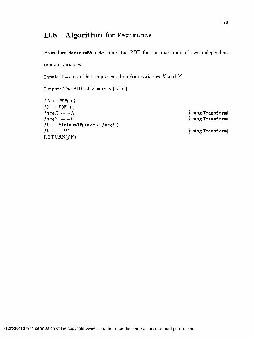
1 7 0

D .8 A lgorith m for MaximumRV

P rocedure MaximumRV determ ines the P D F for th e m axim um of two independent

random variables.

I n p u t: Two list-of-lists represented random variables X and V\

O u tp u t: The P D F of V = m ax {.V. V’}.

f X « - PDF(A) f Y - PDF( Y)f n e g X < X [using T ransform ]f n e g Y < Y [using T ransform ]f V «— MinimumRV(/ne^A*. fnegY')f V < f V [using T ransform ]R E T U R N (/F )

171

D .9 A lgorith m for MLE

Procedure MLE determ ines the m axim um likelihood p aram eter es tim a tes associated

with a random sam ple drawn from a p opu la tion w ith presum ed underly ing d is tribu

tion A\

In p u t: T h e list-of-lists represented ran d o m variable X , th e list of d a ta values s. and

the list of unknow n param eters p.

O utpu t: T h e m axim um likelihood es tim ates of each elem ent in p.

f X — PDF(A')L «— 0 [initialize the log-likelihood function]

" - I M Ifor i *— 1 to n

L *— L + ln ( fX i ' i ( s i ) ) npars « - ||p || for j <— 1 to npars

L'j *— [set up th e derivatives][Using M aple’s s o lv e com m and, solve th e system of equations below]

e q n s e t := -Cseq(L' [ i ] = 0 , i = 1 . . n p a r s ) } ; p a ra m se t := { s e q ( p [ i ] , i = 1 . . n p a r s ) } ; s o ln s := s o l v e ( e q n s e t , p a r a m s e t ) ;

R E T U R N ( s o ln s )

A p pend ix E

A lgorithm for Transform

Introduced in C hapter 3. the following is the algorithm for the T r a n s f orm procedure.

In p u t: The pdf of A'. / ( x ) = f p(x) for zp < x < :p+t, p = 1.2 q.T he tran sfo rm atio n <7 (x) = gt{x) for x, < x < x ,+ i. w here gt{x) is

monotone and not defined piecewise on i , < r < x t+i. and for some p.[Xj.Xt+i] ^ I — 1 .2 ...........71.

Output: The pdf of W h(y) = hj(y) for y: < y < yJ+i, j = 1.2 m.

A “ { x i, X2 -rn+i} [by defin ition . A'* is a sorted list]For i *— 1 to n

FF [i ) «- k [where / ( x ) = f k(x) on (x ,. x 1+1)]If Xi = — cc and x 2 = oc then

ci ^ 0else

B E G I N +- 1 E N D « - n If x x = —oo then

Cj <— Xo — 1B E G I N — 2

If xn+1 = oo thenCn 4 Xn “f- 1E N D <— n — 1

For i <- B E G I N to E N D Ci <— (x, + x ,+ i) /2

172

173

For i *— 1 to na *- limr l r , gdx) b «- limr |Xi+1 g,{x) m t <— m in{a. 6}Mi <— m a x {a . 6}

} ‘ U”=l {m t. .\/,} [V* is a sorted list]m — |V* | - 1

For j <— 1 to m A(y) <- 0 For i <— 1 to n

If m, < i/j and yJ+l < M,Find g~x such th a t g,~l (gi(ci)) = c,h { y ) * - h ( y ) + f F F U ) i g r l ( y ) ) • !^rl(y)l

bj {y) «- h{y)

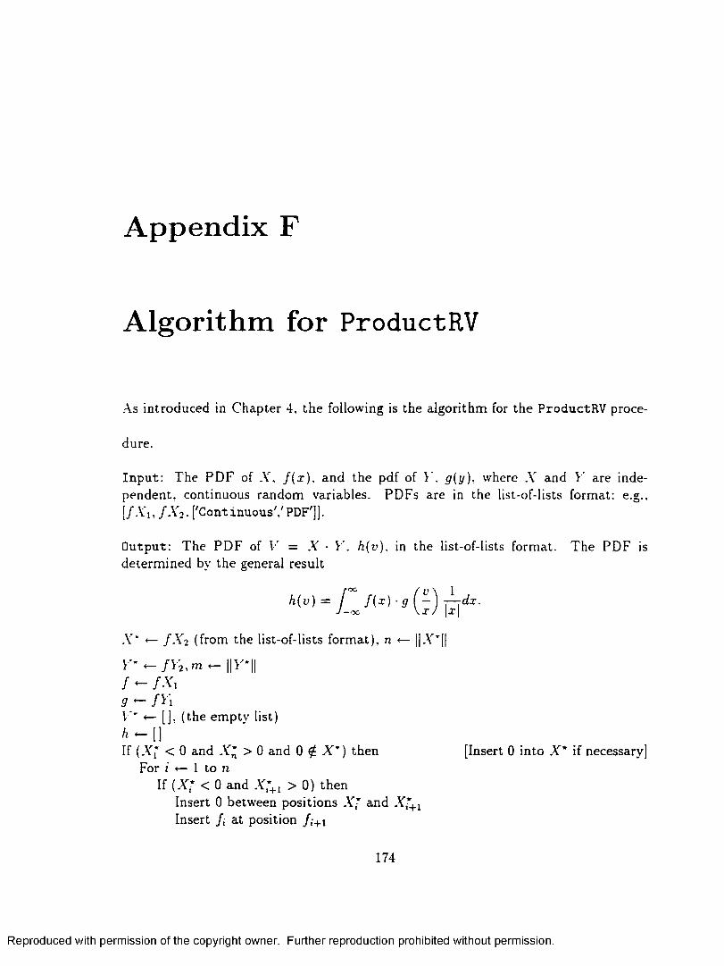
A ppendix F

A lgorithm for ProductRV

As in troduced in C hap ter 4, th e following is the algo rithm for th e P roductR V proce

dure.

In p u t: T he P D F of AC / ( x ) . and the pdf of V’. g(y), where A and Y are independen t. continuous random variables. PD Fs are in the list-of-lists form at: e.g.. [/A ’i, /A C , [ 'C o n tin u o u s ', ' PDF']].

O u tp u t: T he P D F of V = A’ • V. h(v). in the list-of-lists form at. T he PD F is determ ined by th e general resu lt

m = F j w ■ i ( I ) £ ]d i -

X ' <— / AC (from the list-of-lists fo rm at), n <— ||A ''||

Y ' •*— /V 2, m *- ||V '||/ - /AC9 - f Y iV w <— []. ( th e em ptv list)

A- [ ]If (A / < 0 and .V’ > 0 and 0 ^ X *) th en [Insert 0 in to X* if necessary]

For i <— 1 to nIf (X* < 0 and A /+ i > 0) th en

Insert 0 between positions X ' and X*+l Insert / , a t position / , + 1

174

n *— n + 1

breakIf {Y{ < 0 and > 0 and 0 £ V ’ ) then [Insert 0 in to Y ' if necessary]

For i <— I to mIf (>']* < 0 and > 0) th en

Insert 0 betw een positions V]* and ? '+ i Insert <7 , a t position g,+\ m <— m + 1

breakFor i <— I to n [Set up th e suppo rt list I•'’*]

For j *— 1 to mV* «- V" u (X; • V;)

For i *— 1 to / — I h, « - 0

For i «— I to n — I [In teg ra te each segm ent of X tim es each segm ent of >*]For j <— I to m — 1

a <- x ;b - X?+lc - Y ;<1 <- >r+ixy « - A7 • V ;If (-A’ > 0 and x y > 0 ) th en

/ 1 «- f a f i i * ) ■ 9 j i ^ ) ■ [1 st Q uad ran t]If (d < oo) th en f 2 «- J*/d f , ( x ) ■ g ^ ) • \ d xIf (c > 0) th en / 3 - f av/c / , ( x ) • g ^ - ) • ±dxIf (c > 0 and d < oc and ad < be) th en / 4 <— f*jd f ,{x) ■ gj (^ ) • ^dxIf (c = 0 and d = oo) th en [1 st q u ad ran t. Scenario A]

For ii <— 1 to / — 1

If (K* — 0 and Vt'+l < oo) then hu < ha f 1

If (c = 0 and d < oo) th en [1 st q u ad ran t. Scenario B]For ii *— 1 to / — 1

If (KT — 0 ancI KT+i ^ a£f) th en ha < ha -F f 1

If (KT — a£f ancI Ki+i ^ bd) then ha *— ha + / 2

If (c > 0 and d = oo) th e n [1 st q u ad ran t. Scenario C]For ii «— 1 to / — 1

If (KT ^ be and Vj-*+1 < oo) then ha <— ha + / I

If (K ’ — ac an<I K*+i — be) th en ha <— ha + / 3

176

If (c > 0 and d < oo) th en [1 st quad ran t. Scenario D]If (ad < be) th en

For ii <— 1 to / — 1 [1 st Case]If (V' 7 > ac and V£ + 1 < ad) then

h,, <— hi, + / 3 If (V',7 — ad ancI I'u+ 1 — ^c ) then

h,i <— ha + /4 If (V'7 — be an£I liT+i — then

6 ,t «— 6 tI + / 2

If (ad = 6 c) thenFor u <— 1 to / — 1 [2nd Case]

If (V'7 ^ ac ancI Ki+i — Qd) then hi, <— hi, + / 3

If (V'7 — an£I K'7+i — then6 tt <— ha + / 2

If (ad > be) thenFor ii <— I to / — 1 [3rd Case]

If (V] 7 — ac ancI ^ 7 + 1 — ^c ) then h,i *— hi, + / 3

If ( V;; > be and V'*+l < ad) then hi, *- h,i + f 1

If (K7 ^ ancI I77+i — then6 , 1 <— h,, + f'2

If (A7 < 0 and x y > 0) then/ I < fa f.(-r) ■ £ , ( 7 ) • j dx [2nd Q uad ran t]If (d < 0) th en f ’2 *- - t f , d M x ) - ) • I dxIf (c > - 0 0 ) th en / 3 « / al'/c f , ( x ) ■ g}(^) ■ VdxIf (c > —oc and d < 0 and ad > be) then /4 < f f j j f ,{x) ■ gj(^ ) ■ j dxIf (c = —oc and d = 0 ) then [2 nd q u ad ran t. Scenario A]

For ii <— 1 to / — 1

If (V' 7 > 0 and V' * + 1 < 0 0 ) then h„ <— h„ + / I

If (c = —oc and d < 0) then [2nd q u ad ran t, Scenario B]For ii <— 1 to / — 1

If (V' 7 > ad and V'7 + 1 < 0 0 ) then ha <— ha 4- / I

If (K7 ^ ^ ancI Kl+i ^ ac0 thenh,i «— ha + / 2

If (c > — oc an d d = 0 ) th en [2 nd qu ad ran t, Scenario C]For ii *— 1 to / — 1

If (V' 7 > 0 and V£+l < be) th en hi, * ha -f- / I

If (V' 7 > be and Vt'+l < ac) th en

hu * /it'i -F / 3If (c > —oo and d < 0) then [2nd q u ad ran t. Scenario D]

If (ad > be) th enFor ii «— 1 to / — 1 [1st Case]

If (Ii* — a</ an d Kr+t — ac) then hu *- hti + / 3

if (K r — f>c anci Kr+i ^ a£/) thenh-ii *— h-ii + / 4

If (V'7 > bd and V]’+I < be) then flu *— fin + f ~

If (ad = be) th enFor ii «— 1 to / — I [2nd Case]

If > ad and V'*+1 < ac) then fin i— fin + / 3

If (KT ^ bd and V[*+i < 6c) then ha *— fiu + / 2

If {ad < be) th enFor ii <— 1 to / — I [3rd Case]

If 077 > be ancI K7+i ^ ac) thenhu *— hu + / 3

If 077 ^ Qd an<f Kr+i ^ be) then fiu *— ha + / I

If 077 > bd and V'*+1 < ad) then flu *— flit + f ~

If (.V,’ < 0 and xy < 0) then/ 1 < la f ‘(T ) ■ 9 j{^) ■ j dx [3rd Q uadran t]If (d < oc) then / 2 < f ”/d f t{x) ■ £ ,(;) • jd xIf (c > 0) then / 3 «------/„6/c / , ( x ) ■ &■(£) • ^dx

If (c > 0 and d < oo and 6d > cc) then /4 -<------ / , ( x ) • g}{ j ) • jd xIf (c = 0 and d = oo) th en [3rd q uad ran t. Scenario A]

For ii «— I to / — 1If 077 - ancI I’u+i — 0) then

fiu *— hu + / IIf (c = 0 and d < oo) th en [3rd q uad ran t. Scenario B]

For ii <— I to / — 1If (K7 ^ bd and V ’+i < 0) then

fiu +— hi i + / 1 If (K7 — °-d and V'’+1 < bd) then

hu +— hu + f ~If (c > 0 and d = oo) th en [3rd q u ad ran t. Scenario C]

For ii -*— 1 to / — 1If 077 — ~ ° ° ancI K7+ 1 ^ ac) then

hu <— hu + / I

ITS

If ( I i! > ac and V'7 + 1 < be) then hu < /ijt 4* f 3

If (c > 0 and d < oo) then [3rd q u ad ran t. Scenario D]If (bd > ac) then

For ii «— 1 to / — 1 [1 st Case]If ( V' 7 > bd and V' * + 1 < be) then

hu *— h„ + / 3 if ( f i r ^ ac an<i Kr+i — hd) then

hii <— hti + / 4 if ( i jr — aRci k t+ i — a c ) then

h,t <— ha + / 2 If (ac — bd) then

For ii <— 1 to / — 1 [2nd Case]

If (KT — ad an(I Ki+i — a c ) then htt <— h,, + f'2

If (I-]' > bd and V[ * + 1 < be) then hu hu + / 3

If (ac > bd) thenFor H i— 1 to / — I [3rd Case]

If (Ct’ > ac and V'*+l < be) then h„ <— hu + / 3

If ( V > bd and V' * + 1 < ac) thenhu <— hti + / I

If (Vi; > nd and Vt'+l < bd) then h„ i— hi, + f'2

If (-V' > 0 and xy < 0 ) then/ 1 fa M x ) • 9 j i ^ ) • jd x [4th Q u ad ran t]If (d < 0) th en f'2 4- f* /d f , ( x ) ■ g: (^) • x-dx If (c > - o c ) th en / 3 f*f e f t(x) • g}(^) ■ ^dxIf (c > —oc and d < 0 and ac > bd) then / 4 <— f ”j d / , ( x) ■ g}( • ^dxIf (c = —OC' and d = 0) then [4th q u ad ran t. Scenario A]

For ii 4— 1 to / — 1If (KT ^ — 0 0 ancI K’+i ^ 0 ) then

h,t 4— h„ + f IIf (c = —oc and d < 0) th en [4th q u ad ran t, Scenario B]

For ii <— 1 to / — 1If (K* ^ ~ 0 0 ancI I w , 5: hd) then

hn 4— h„ + / I If (KT — hd and V'[’+ i — fld) then

h„ 4— h„ + f ’2If (c > — 0 0 and d — 0) th en [4th q u ad ran t, Scenario C]

For ii 4— 1 to / — 1

If (KT — ac an£I KT+i — 0) then

h„ <— ha 4 - /1 If (V'J > be and V'*+l < ac) then

ha «— ht{ 4- / 3 If (c > —oc and d < 0) then

If (ac > bd) then For ii <— 1 to / — 1

If (K r — he and V''+1 < bd) th en hu <— h^ 4- /3

If (Ii,' > bd and V’Tn < ac) th en h„ «— ha ■+- /4

if ( i , r ^ ac anci Kr+i ^ ac0 th en hi, *— hu 4- f'2

If (ad = be) then For ii *— 1 to / — 1

If (I[7 > be and 1 7 7 + 1 5: ac) th e n h„ <— hu 4- / 3

If ( I i ’ ^ ac ancI I|7+i < ad) th en h„ <— hu 4- f'2

If (ac < bd) then For ii «— 1 to / — 1

If (V'; > be and V-’+1 < ac) then h„ '— h,t 4- / 3

If ( I ,r ^ ac ancI Kr+i ^ hd) th en h„ <— h,, + / I

If (I'w — hd and V''+1 < ad) th en h t, <— hu 4- f ’2

f \ i - h f \ ’i - I "f \ 3 «- [ 'Continuous'. ' PDF']R etu rn ( /V )

[4th quad ran t. Scenario D]

[1st Case]

[2nd Case]

[3rd Case]

[M ake a new list-of-lists for V']

A ppendix G

A lgorithm for KSRV

Procedure KSRV: C om puting the C D F of the K olm ogorov-Sm irnov te st s ta tis tic .

when all p a ram eters are known.

O u tp u t: T h e C D F of the KS test s ta tis tic when all param eters a re known is re tu rn ed . T he random variable will be in the usual list-of-lists form at.

[P h a s e 1: D eterm ine the endpoin ts of th e segm ents th a t define the support of th e KS test s ta tis tic .]

In p u t: A positive integer n. the sam ple size associated w ith the KS test s ta tis tic

D im ension v 0 [r holds th e partition values for the support of D n]

9z 2 n IFor i *— I to n — 1 by 1

m «— 777 + 1

[g is th e gap betw een adjacent in teg ra tion lim its when v = 0]

I’m <— I - gFor j <— 2 • LfJ + 1 to 2n — 1 by 2 [Lower lim it is n o r n + 1, whichever is odd]

777 + 1

[P h a s e 2: T h e next phase of the a lg o rith m has th ree parts to it.

1. Define c i ,c 2 cm as the m idpo in ts of the support in tervals

ISO

1S1

2. Define x i , x 2 x„ as the lim its of in tegration when v = 0

3. Define th e n x n ind icato r m atrices A i, A2, • • • . Am.]

Dimension c[m]For k 1 to m

cfc ♦- + v k)/2

Dimension x[n]For i *— 1 to n

x, <- (2 i - 1) • g

Dimension A[n, n]

For i <— 2 to nFor j «— 1 to i — 1

A0 « - 0

For k *— I to m For i <— 1 to n

For j <— i to nA.J - 0

[Define vector c of m idpoints of the su p p o rt subintervals]

[Define vector x of centers of in teg ra tion limits]

[Zero ou t lower triang le of .4]

[Loop through all su b in te rva ls of support]

x <- m a x ][n e t - 5 J.O}I <— min { [2 ncfc"|. n}

f e ” V' 2^ + u)]For 1 *— 1 to n

For j <— m ax{i. z + 1} to m in{n. i + / — 1}

[Zero ou t u p p er triang le of .4] [z is th e num ber of leading zero colum ns in .4]

[/ is the num ber of u -sub in terva ls th a t in tersect

4 , [Place l 's in 4]

[P h a s e 3: C om pute th e fixed and variable lim it m atrices F and V and com bine to give the piecewise polynom ial CDF]

Dimension P[m\ [nth order polynom ials for CD F segm ents, p a ram eterized by u] Dimension P fn , n] [A rray of Fixed integrals, p a ram eterized by u]Dimension V'[n, n] [A rray of Variable integrals, p a ram eterized by u]Real S[v) [A function of v, used as a runn ing sum]

[S(t>) is th e sum of all F elem ents one row down, s ta rtin g one e lem en t to th e right]

Pi(v) *— n!(2u)n For k *— 2 to m

z <- m a x ][n e t - ±J.O} / ♦— min { f2 n c^ ], n} Fn,n(v) *- 1 dunVn.n{v) *- t . , 1 dun

[/>,<») - » ! • ■ ■ c r 1 i U;[Loop through ail su b in te rva ls of support

1S2

For i <— n — 1 to 2 by — 1 If i + / > n then

5 ( f ) «— 0else

5 ( f ) «- Fi+u+i(v)If i + / > n + 1 then

K M - J+(X|+u,( 1 “Lx'+CfcJ) Vi+Uv)duiVi.n(v) - f £ ? C k V;+I n(ll) dUi

If i -I- / = n + 1 thenF U v ) ^ ri 'tX l V ^ . n { v ) d u x

If f + / < n + I thenF i M - t i v ) - {K +lii+,_,(*,) + 5 ( f ) } dm

5 ( f ) — 5 ( f ) + 5 t+1,min{i+/_ 1,n}( f )For j <— m in{n — I , i + [ — 2} to m ax{i + 1 .c + 2} by —1 [Interior of .4 m atrix]

Fi.Av) I x ’- 1v~V {V i+ i.j(f) + 5 ( f )} dmK j i v ) ^ i z : r v W + i d W + S (v)}5 ( f ) «- 5 ( f ) + Ft+Uj{v)

If r + I i thenV,.z+i{v) «- ! ^ z*l2~v {V;+1,-+1(f) + 5 ( f )} du,

If r 4- I < i thenF , . , ( v )< - f rT: : r s ( v ) d u t

If l = n then [Rows 2 .3 n of A m a trix com pleted a t th is point]5 ( f ) - 0F i M ' ) ^ £'nl : . V 2 A v ) d u x

else5 ( f ) — F 2,/+i( f )

If / < n thenF \,i( f ) « - Ixt'-J { V-u( f ) + 5 ( f )} dui

5 ( f ) < - 5 ( f ) + F 2 j ( v )

For j <— m in{n — 1. / — 1} to m ax{2. - + 1} bv — 1FuAv) - m . ^ ) + 5 (f )} dm5 ( f ) <- 5 ( f ) + F2,j {v )

If r = 0 thenFi.i{v) *- / 0X5_l’ 5 ( f ) dui

Pk( v ) * - 0 For j *— z + L to /

Pk(v) <- Pk(v) + F i j (v )Pk(v) *- n\Pk{ f )

1S3

[ P h a s e 4: Shift the d is tr ib u tio n to th e form of P {D n < y) by su b s titu tin g y = +

2/o <— v0 + 2kFor k <— 1 to m [Loop th ro u g h all sub in tervals of support]

y . - Vk + £Fk{y) *- Pk{y - £ )

R e tu r n : y0, y u . . . , y m and F x(y), F2(y), ■.. , F m(y).

A ppendix H

Sim ulation C ode for MLEOS

A pproxim ations

As ou tlined in C h ap te r 7. th e following M aple code was used to generate the M LEO S

versus MLE estim ations for 6 from the U niform (0. 9) d is tribu tion . T he p rocedu re

S e c S o lv e is a generic secan t-m ethod for finding num erical solutions to an eq u a

tion. This procedure is faster in finding solu tions to th e MLEOS equation th a n

M aple 's f s o lv e com m and. T he procedure M a x In itV a ls is a p reparato ry p rocedu re

for S ec S o lv e th a t re tu rn s an interval w here a local m axim um can be found. It is

m erely a grid-search of an in terval to find tw o poin ts x t < x-i such th a t f ' ( x i) > 0 >

f ’( x 2 ). which is a cond ition for a local m ax im um on / ( x ) on [X1 .X 2 ].

r e s t a r t ;r e a d ( ' d : / r e s e a r c h /p r o b m a p /p r o b p r o c .m a p ' ) ; r e a d C fd : / r e s e a r c h / s e c a n t . m a p ') ; r e a d ( 'd : / r e s e a r c h / m a x i n i . m a p ') ;

1S4

n t e s t := 1000; nsample := 25; D i g i t s := 10;Seed := r e a d l i b ( r a n d o m i z e ) 0 ; random ize (8218); o u t p t := a r r a y ( l . . n t e s t ) ; t h i s d i s t := UniformRV(0, b ) ; bsample := 1;f o r i from 1 t o nsample do

fnow [ i ] := O r d e r S t a t ( t h i s d i s t , nsample, i ) : od:varsam ple := a r r a y (1 . . n sam ple) ; w incn t := 0;f o r k from 1 t o n t e s t do

p r i n t ( k i s n o w , k ) ; f o r i from 1 t o nsample do

v a r s a m p le [ i ] := e v a l f ( V a r U n i ( 0 .0 , b s a m p l e ) ) ; od;v a r l i s t := s o r t ( [ s e q ( v a r s a m p l e [ i ] , i = 1 . . n s a m p l e ) ] ) ; b o ld := v a r l i s t [ n s a m p l e ] ;11s := 0;f o r i from 1 t o nsample do

11s := 11s + l n ( f n o w [ i ] [ l ] [ l ] ( v a r l i s t [ i ] ) ) : o d :l i s p := u n a p p l y ( ( d i f f ( 1 1 s , b ) ) , b ) : bnew := S e c S o l v e ( l l s p , 0 .9 9 8 , 0 .9 9 6 ) : i f (bnew = bad) t h e n

i n i := M a x I n i t V a l s ( l i s p , 0 .0 2 , 2 . 2 , 5 ) ; p r i n t ( ‘ i n i t i a l g u e s s e s a r e i n i [ l ] , i n i [2 ] ) ; bnew := S e c S o l v e ( l l s p , i n i [ l ] , i n i [ 2 ] ) ;

f i ;i f (bnew = bad) th e n bnew := v a r l i s t [ n s a m p l e ] ;e l i f (abs(bnew - 1) > a b s ( l - v a r l i s t [ n s a m p l e ] ) ) t h e n

bnew := v a r l i s t [ n s a m p l e ] ; e l s e

wincn t := w incn t + 1; p r i n t ( w i n c n t ) ;f i ;o u t p t [k] := [bnew, b o l d , b o ld * (nsample + 1) / nsample]

o d :suml := 0; sum2 := 0; sum3 := 0; v a r l := 0; var2 := 0; v a r3 := 0; sk ip p ed := 0; f o r i from 1 t o n t e s t do

i f ( n o p s ( o u t p t [ i ] ) = 3) t h e n


1S6

o u t p t [ i ] [1 ] ; ( o u t p t [ i ] [ l ] o u t p t [ i ] [2 ] ; ( o u t p t [ i ] [2] o u t p t [ i ] [3 ] ; ( o u t p t [ i ] [3]

bsample )

bsample )

bsample )

1;

suml := suml + v a r l := v a r l + sum2 := sum2 + v a r2 := var2 + sum3 := sum3 + v a r3 := var3 +

e l s es k ip p e d := s k ip p ed +

f i ;o d :p r i n t ( ' s i z e of each sample =

'number of samples = avenew := suml / ( n t e s t -av e o ld := sum2 / ( n t e s t -avgadj := sum3 / ( n t e s t -varnew := v a r l / ( n t e s t -v a r o l d := var2 / ( n t e s t -v a r a d j := var3 / ( n t e s t -p r i n t ( ' h a d to s k i p ' , s k ip p e d , 'win p e r c e n t a g e = ‘

e v a l f ( w i n c n t / ( n t e s t - s k i p p e d ) ) ) ;

n sam ple ,' , n t e s t ) sk ipped) sk ipped ) sk ipped ) sk ipped ) sk ipped ) sk ipped )


B ibliography

[1] B alakrishnan, N. and W . W. S. Chen, 1997. C R C Handbook o f Tables fo r Order Statistics f rom Inverse Gaussian Distributions with Applications. New York: CRC.

[2] Barlow. R. E. a n d F. P roschan, 1981. Statistical Theory o f Reliability and Life Testing. Silver Spring . M d.: To Begin W ith .

[3] B arr. D. R.. 1994. Personal com m unication.

[4] B arr. D. R. and T . Davidson. 1973. “A K olm ogorov-Sm irnov Test for C ensored Sam ples." Technometrics. Volume 15. pp. 739-757.

[5] B arr. D. R. and P. W . Zehna. 19S3. Probability: Modeling Uncertainty. R eading. Mass.: A ddison-W esley.

[6] B arr. D. R. a n d P. W. Zehna. 1971. Probability. B elm ont. California: B rooks- C’ole.

[7] Berger. R., 1995. Personal com m unication.

[8] B irnbaum . Z. W .. 1952. ‘'N um erical T ab u la tio n of th e D istribu tion of Kolo- m ogorov's S ta tis tic for F in ite Sample Size." Journal o f the American Statistical Association. V olum e 47. pp. 425-441.

[9] Casella, G. and R. Berger. 1990. Statistical Inference. Pacific G rove, C alifornia: W adsw orth and B rooks/C ole . Inc.

[10] C hhikara, R. S. and Folks. L. S.. 19S9. The Inverse Gaussian Distribution: Theory, Methodology and Applications. New York: M axcel Dekker.

[11] Cox, D. R. and D. O akes, 1984. Analysis o f Survival Data. New York: C hapm an and Hall.

187


1SS

[12] Cox. D. R. and E. J . Snell. 1981. Applied Statistics. New York: C h ap m an and Hall.

[13] Crowder. M. J .. A. C. K im ber. R. L. S m ith and T . J. Sw eeting. 1991. Statistical Analysis o f Reliability Data. New York: C hapm an and Hall.

[14] D’Agostino. R. B. and M. A. S tephens. 19S6. Goodness-of-Fit Techniques. New York: M arcel Dekker.

[15] David. H. A.. 1981. Order Statistics. Second edition. New York: Jo h n W iley and Sons.

[16] David. H. A.. 1993. "A N ote on O rd er S ta tis tic s for D ependent V ariab les." Journal of the American Statistical Association. Volume 47. pp. 198-199.

[17] Devrove. L.. 1996. ^R andom V ariate G eneration in O ne Line of C ode." from Proceedings o f tht 1996 Winter Simulation Conference. J . C h arnes . D. M orrice, D. B runner, and J. Swain, eds. C oronado, California: In s titu te of E lec trica l and Electronics Engineers, pp. 265-272.

[18] Evans. .VI.. N. H astings and B. Peacock, 1993. Statistical Distributions. Second edition. New York: John W iley and Sons.

[19] Freund. J .. 1992. Mathematical Statistics. F ifth edition. Englew ood Cliffs. New Jersey: P ren tice-H all.

[20] G ehan. E. A.. 1965. “A G eneralized W ilcoxon Test for C om paring A rb itra rily Singly-Censored Sam ples." Biometrika. Volume 52. P arts I and 2. pp. 203-223.

[21] H arter. H. L. and N. B alakrishnan . 1996. C RC Handbook o f Tables fo r the Use of Order Statistics in Estimation. New York: CRC.

[22] Hogg. R. V. and A. T . C raig. 1995. Mathematical Statistics. F if th ed itio n . Englewood Cliffs. New Jersey: P ren tice -H a ll.

[23] Johnson. N. L., S. K otz, and N. B alakrishnan , 1995. Continuous Univariate Distributions. Volume 2, Second ed itio n . New York: John W iley an d Sons.

[24] Johnson, R. A. and D. W . W ichern, 1992. Applied Multivariate Statistical Analysis. T hird ed ition . Englewood Cliffs, New Jersey: P ren tice -H all.

[25] Kececioglu, D.. 1991. Reliability Engineering Handbook. Volume I. Englew ood Cliffs. New Jersey: P ren tice-H all.

[26] K endall, M. G .. and A. S tu a rt, 1963. The Advanced Theory o f Statistics: Volume II Inference and Relationship. New York: H afner Publishing.

[27] K nuth , D. E.. 1981. The Art o f Computer Programming, Second ed itio n . R eading, Mass.: A ddison-W esley.


1S9

[28] K uiper, N. H.. 1960. “T ests C oncerning R andom Points on a C ircle." Proc. Koninkljke Nederlandse Akadamie van Wetenschappen. Series .4. Volume 63. pp. 38-47.

[29] Larsen, R. J . and M. L. M arx. 1986. An Introduction to Mathematical Statistics and Its Applications, Second ed ition . Englewood Cliffs. New Jersey : P ren tice - Hall.

[30] Law. A. M. and YV. D. K elton. 1991. Simulation Modeling and Analysis. Second edition . New York: M cG raw -H ill.

[31] Lee, E. T .. 1992. Statistical Methods fo r Survival Data Analysis, Second edition. New York: John YVilev and Sons.

[32] Lee, S.. J . R. W ilson, and M. M. C raw ford, 1991. “M odeling and S im ulation of a Nonhom ogeneous Poisson Process w ith Cyclic Features." Communications in Statistics - Simulation and Computation. Volume 20, pp. 777-809.

[33] Leemis, L.. 1995. Probabilistic Models and Statistical Methods in Reliability. Englewood Cliffs. New Jersey: P ren tice -H all.

[34] Lehm ann, E. L.. 1986. Testing Statistical Hypothesis, Second ed itio n . New York: John W iley and Sons.

[35] Lieblein. J . and M. Zelen, 1956. “S ta tis tic a l Investigation of th e Fatigue Life of D eep-G roove Ball B earings." Journal o f Research of the National Bureau of Standards. Volume 57, pp. 273-316.

[36] Lilliefors. H. W .. 1967. “On th e K olm ogorov-Sm irnov Test for N o rm ality w ith Mean and V ariance Unknow n." Journal of the American Statistical Association. Volume 62. pp. 399-402.

[37] Lilliefors, H. W .. 1969. “On th e K olm ogorov-Sm irnov Test for th e E xponential D istribu tion w ith M ean U nknow n.” Journal o f the American Statistical Association. Volume 64. pp. 387-389.

[38] M iller. L. H., 1956. “Table of P ercen tage Poin ts of Kolmogorov S ta tis tic s .” Journal o f the American Statistical Association. Volume 51. pp. 111-121.

[39] M oore. D. S. and G. P. M cC abe, 1993. Introduction to the Practice o f Statistics , Second edition . New York: W . H. F reem an and Company.

[40] Owen. D. B., 1962. Handbook o f Statistical Tables. R eading, M ass.: A ddison- Wesley.

[41] Park . S. and L. M. Leemis, 1997. Discrete-event Simulation: A First Course. The College of YY’illiam M ary.


1 9 0

[42] Port. S. C .. 1994. Theoretical Probability for Applications. New York: John W iley and Sons.

[43] Rohatgi. V. K.. 1976. .4n Introduction to Probability Theory and Mathematical Statistics. New York: John W iley and Sons.

[44] Ross. S. M., 1993. Introduction to Probability Models. F ifth ed ition . B oston: Academ y Press.

[4-5] Sahner. R. A. and K. S. T rivedi. 1993. UA Softw are Tool for Learning A bo u t Stochastic M odels." IE EE Transactions on Education. V olum e 36. pp. 56-61.

[46] Sarhan A. E. and B. G. G reenberg , 1962. Contributions to Order Statistics. New York: John W iley and Sons.

[47] Stephens. M. A.. 1965. l'T h e G oodness-of-fit S ta tis tics: D istribu tions and Significance Poin ts." Biometrika. Volume 52. pp. 309-322.

[45] S tephens. M. A.. 19S6. "Tests Based on EDF S ta tis tic s ." from Goodness-of-fit Test Techniques. R. B. D A gostino and M. A. S tephens, eds. New York: M arcel Dekker. pp. 97-193.

[49] T ietjen , G. L.. 1986. "The A nalysis and D etection of O u tlie rs ." from Goodness- of-fit Techniques. R. B. D ’A gostino and M. A. S tephens, eds. New York: M arcel Dekker. pp. 497-522.

[50] Trivedi. K. S.. 1997. Personal com m unication.


Vita

A ndrew G ordon Glen is a M ajor in th e U nited S ta tes A rm y, c u rre n tly assigned as an

ass is tan t professor in th e D ep artm en t of System s E ngineering a t th e U nited S ta te s

M ilitary A cadem y in W est P o in t, New York. He was born on F eb ruary 22. 1962

in Denville, New Jersey. He holds a Bachelors of Science degree, g rad u a ted and

com m issioned in th e F ield A rtillery by the U nited S ta tes M ilita ry A cadem y in 19S4.

He also holds a M asters of Science degree from the College of W illiam k M ary,

g rad u a ted in 1995. He is a career A rm y officer of 14 years who has served num erous

overseas tours, to include com bat d u ty in th e Persian Guif. His m ilita ry aw ards

include the Bronze S ta r and the M erito rious Service M edal w ith O ak Leaf C luste r.

He is m arried to th e form er Lisa M ary S tew art, now also a M ajor in th e Army. T he

G lens have th ree daugh ters. A ndrea . R ebecca, and Mary.

191


* v%,

b„

v*

IMAGE EVALUATION TEST TARGET (G A -3 )

✓

A

1.0

l . l

1.25

|« ■ 2.8 Li£US U £

U14.0

1.4

\M2.2

2.0

1.8

1.6

150mm

A P P L IE D A IIVU4GE . Inc1653 East Main Street

■ Rochester, NY 14609 USA _ = Phone: 716/482-0300

- ^ = ~ - = = = Fax: 716/288-5989

C 1993. Applied Image, Inc.. All Rights Reserved

permission of the copyright owner. Further reproduction prohibited without permission.

a probability programming language: development and

Documents