a probabilisitic based failure model for …academic.csuohio.edu/duffy_s/chengfeng xiao dissertaton...
TRANSCRIPT

A PROBABILISITIC BASED FAILURE MODEL FOR
COMPONENTS FABRICATED FROM ANISOTROPIC
GRAPHITE
CHENGFENG XIAO
Bachelor of Science
Sun Yat-Seng University, Guangzhou, China, 2001
Master of Mechanical Engineering
Sun Yat-Seng University, Guangzhou, China. 2004
Submitted in partial fulfillment of the requirements for the degree
DOCTOR OF ENGINEERING
At the
CLEVELAND STATE UNIVERSITY
April 2014
We hereby approve the dissertation of
Chengfeng Xiao
Candidate for the Doctor of Engineering degree.
This dissertation has been approved for the Department of
CIVIL AND ENVIRONMENTAL ENGINEERING
and CLEVELAND STATE UNIVERSITY
College of Graduate Studies by
Stephen F. Duffy PhD, PE, F.ASCE - Dissertation Committee Chairman Date
Department of Civil and Environmental Engineering
Lutful I. Khan PhD, PE - Dissertation Committee Member Date
Department of Civil and Environmental Engineering
Mehdi Jalalpour PhD - Dissertation Committee Member Date
Department of Civil and Environmental Engineering
Miron Kaufman PhD - Dissertation Committee Member Date
Department of Physics, College of Sciences and Health Professions

John P. Gyekenyesi PhD, PE, F.ACerS - Dissertation Committee Member Date
NASA Glenn Research Center (retired)
Paul A. Bosela PhD, PE, F.ASCE - Dissertation Committee Member Date
Department of Civil and Environmental Engineering (retired)
Student’s Date of Defense
This student has fulfilled all requirements for the Doctor of Engineering degree.
Dan Simon PhD - Doctoral Program Director

iv
ACKNOWLEDGMENTS
This academic project used up many of weekend and vacations, which I would
normally have spent with my family and it is indeed extremely difficult to acknowledge
their sacrifice. I wish to acknowledge the love and support I received from my wife,
Xiang Li, during the duration of this project. I wish to note a deep and special
gratitude to my parents, Yougang Xiao and Meifen Liang, for their patience and
understanding. In addition, I wish to thank my brothers, Chengjun and Chenghao, and
sister, Chengxia for your gentle encouragement.
Next, I wish acknowledge how indebted I am to my dissertation committee
chairman and graduate advisor Dr. Stephen Duffy. He provided the seed ideas for the
efforts outlined in this dissertation. He was patient and provided encouragement as well
as advice when I needed it. I am grateful and proud to be one Dr. Duffy’s students.
I also want to recognize the generous support received from the United States
Department of Energy (DoE), and I especially wish to thank the technical point of contact
(POC) Dr. Rob Bratton at the Idaho National Laboratory (INL). My efforts were
supported under DoE Contract Number 00088589, Project #09-347 entitled “Modeling
Stress Strain Relationships and Predicting Failure Probabilities For Graphite Core

v
Components.” Many thanks to Dr. Timothy Burchell at ORNL for the use of his
graphite data. It was an honor to be associated with the great minds and wonderful talent
at both INL and the Oak Ridge National Laboratory (ORNL).
vi
A PROBABILISITIC BASED FAILURE MODEL FOR
COMPONENTS FABRACATED FROM ANISOTROPIC
GRAPHITE
CHENGFENG XIAO
ABSTRACT
The nuclear moderator for high temperature nuclear reactors are fabricated from
graphite. During reactor operations graphite components are subjected to complex
stress states arising from structural loads, thermal gradients, neutron irradiation damage,
and seismic events. Graphite is a quasi-brittle material. Two aspects of nuclear grade
graphite, i.e., material anisotropy and different behavior in tension and compression, are
explicitly accounted for in this effort. Fracture mechanic methods are useful for metal
alloys, but they are problematic for anisotropic materials with a microstructure that
makes it difficult to identify a “critical” flaw. In fact cracking in a graphite core
component does not necessarily result in the loss of integrity of a nuclear graphite core
assembly. A phenomenological failure criterion that does not rely on flaw detection has
been derived that accounts for the material behaviors mentioned. The probability of
failure of components fabricated from graphite is governed by the scatter in strength.
The design protocols being proposed by international code agencies recognize that design
vii
and analysis of reactor core components must be based upon probabilistic principles.
The reliability models proposed herein for isotropic graphite and graphite that can be
characterized as being transversely isotropic are another set of design tools for the next
generation very high temperature reactors (VHTR) as well as molten salt reactors.
The work begins with a review of phenomenologically based deterministic failure
criteria. A number of this genre of failure models are compared with recent multiaxial
nuclear grade failure data. Aspects in each are shown to be lacking. The basic
behavior of different failure strengths in tension and compression is exhibited by failure
models derived for concrete, but attempts to extend these concrete models to anisotropy
were unsuccessful. The phenomenological models are directly dependent on stress
invariants. A set of invariants, known as an integrity basis, was developed for a
non-linear elastic constitutive model. This integrity basis allowed the non-linear
constitutive model to exhibit different behavior in tension and compression and
moreover, the integrity basis was amenable to being augmented and extended to
anisotropic behavior. This integrity basis served as the starting point in developing both
an isotropic reliability model and a reliability model for transversely isotropic materials.
At the heart of the reliability models is a failure function very similar in nature to
the yield functions found in classic plasticity theory. The failure function is derived and
presented in the context of a multiaxial stress space. States of stress inside the failure

viii
envelope denote safe operating states. States of stress on or outside the failure envelope
denote failure. The phenomenological strength parameters associated with the failure
function are treated as random variables. There is a wealth of failure data in the
literature that supports this notion. The mathematical integration of a joint probability
density function that is dependent on the random strength variables over the safe
operating domain defined by the failure function provides a way to compute the
reliability of a state of stress in a graphite core component fabricated from graphite. The
evaluation of the integral providing the reliability associated with an operational stress
state can only be carried out using a numerical method. Monte Carlo simulation with
importance sampling was selected to make these calculations.
The derivation of the isotropic reliability model and the extension of the reliability
model to anisotropy are provided in full detail. Model parameters are cast in terms of
strength parameters that can (and have been) characterized by multiaxial failure tests.
Comparisons of model predictions with failure data is made and a brief comparison is
made to reliability predictions called for in the ASME Boiler and Pressure Vessel Code..
Future work is identified that would provide further verification and augmentation of the
numerical methods used to evaluate model predictions.
ix
TABLE OF CONTENTS
ACKNOWLEDGMENTS ................................................................................................ IV
ABSTRACT ...................................................................................................................... VI
LIST OF NOMENCLATURE ......................................................................................... XII
CHAPTER I GRAPHITE COMPONENTS IN NUCLEAR REACTORS ..................... 1
1.1 Research Objectives ........................................................................................ 5
CHAPTER II STRENGTH BASED FAILURE DATA .................................................. 9
2.1 Integrity Basis ............................................................................................... 10
2.2 Useful Invariants of the Cauchy and Deviatoric Stress Tensors ................... 13
2.3 Graphical Representation of Stress ............................................................... 15
2.4 Graphite Failure Data .................................................................................... 18
2.5 The von Mises Failure Criterion (One Parameter) ....................................... 21
CHAPTER III TWO AND THREE PARAMETER FAILURE CRITERIA ................ 28
3.1 The Drucker-Prager Failure Criterion (Two Parameter) .............................. 28
3.2 Willam-Warnke Failure Criterion (Three Parameter) ................................... 45

x
CHAPTER IV ISOTROPIC FAILURE CRITERION FOR GRAPHITE ..................... 59
4.2 Integrity Basis and Functional Dependence ................................................. 60
4.3 Functional Forms and Associated Gradients by Stress Region .................... 61
4.4 Relationships Between Functional Constants ............................................... 69
4.5 Functional Constants in Terms of Strength Parameters ................................ 77
CHAPTER V ANISOTROPIC FAILURE CRITERION .............................................. 87
5.1 Integrity Base for Anisotropy ....................................................................... 88
5.2 Functional Forms and Associated Gradients by Stress Region .................... 89
5.3 Relationships Between Functional Constants ............................................... 96
5.4 Functional Constants in Terms of Strength Parameters .............................. 120
CHAPTER VI MATERIAL STRENGTH AS A RANDOM VARIABLE................. 149
6.1 Integration by Monte Carlo Simulation ...................................................... 156
6.2 The Concept of Importance Sampling Simulation ...................................... 164
6.3 Isotropic Limit State Function – Importance Sampling .............................. 175
6.4 Anisotropic Limit State Functions – Importance Sampling ....................... 184
xi
CHAPTER VII SUMMARY AND CONCLUSIONS ................................................ 192
7.1 Comparison With the ASME Simplified Assessment Method ................... 193
7.2 Theoretical Development - Summary ......................................................... 208
7.3 Conclusions and Future Efforts .................................................................. 211
REFERENCES ............................................................................................................... 214
xii
NOMENCLATURE
ai unit vector aligned with principal stress direction
di unit vector aligned with preferred material direction
e unit vector aligned with the hydrostatic stress line
Yf probability density function of a random strength variable characterized by a two
parameter Weibull distribution
YF cumulative probability density function of a random strength variable
characterized by a two parameter Weibull distribution
g general failure criterion function
gi failure function associated with principal stress region “i”
I indicator function
I transformed indicator function
I1 first invariant of the Cauchy stress tensor
I2 second invariant of the Cauchy stress tensor
I3 third invariant of the Cauchy stress tensor
J1 first invariant of the deviatoric stress tensor
J2 second invariant of the deviatoric stress tensor
J3 third invariant of the deviatoric stress tensor
xiii
Yk importance sampling density function
YK cumulative importance sampling density function
m Weibull modulus
Pf probability of failure
r deviatoric component of a stress state
R reliability
Rtc the ratio of the mean compressive strength to the mean tensile strength
S deviatoric principal stress
Sij deviatoric stress tensor
y realization of a random strength parameter
Y random strength parameters
Z standard normal random strength variables
ij Kronecker delta tensor
Lode angle in the deviatoric stress plane
Y standard deviation of a random strength parameter
Yf standard deviation of the Weibull distribution
Yk standard deviation of the importance sampling function
Y mean of a random strength variable
Yf the mean of the Weibull distribution
xiv
Yk mean of the importance sampling function
ij Cauchy stress tensor
i principal stress
Weibull characteristic strength
T tensile strength parameter
C compressive strength parameter
BC equal biaxial compressive strength parameter in the plane of isotropy
TT tensile strength parameter in the plane of isotropy
TC compressive strength parameter in the plane of isotropy
YT tensile strength parameter in the preferred material direction
YC compressive strength parameter in the preferred material direction
MBC equal biaxial compressive strength parameter with one stress component in the
plane of isotropy
v equivalent stress as defined by ASME
hydrostatic component of a stress state
Poisson’s ratio
joint probability density function of material strength parameters

1
CHAPTER I
GRAPHITE COMPONENTS IN NUCLEAR REACTORS
As discussed by Saito (2010) nuclear energy plays an important role as a means to
secure a consistent and reliable source of electricity that can easily help utilities meet
system demand for the nation’s power grid and do so in a way that positively impacts
global warming issues. Proposed system designs for nuclear power plants, e.g., the
Generation IV Very High Temperature Reactors (VHTR) (2002) among others, will
generate sustainable, safe and reliable energy. The nuclear moderator and major
structural components for VHTRs are fabricated from graphite. During operations the
graphite components are subjected to complex stress states arising from structural loads,
thermal gradients, neutron irradiation damage, and seismic events, any and/or all of which
can lead to failure. As discussed by Burchell et al. (2007) failure theories that predict
reliability of graphite components for a given stress state are important.
Graphite is often described as a brittle or quasi-brittle material. An excellent
overview of advanced technology applications involving the use of graphite material as
2
well as the unique behavior of this carbon based material can be found in Burchell (1999).
Tabeddor (1979) and Vijayakumar, et al. (1987, 1990) emphasize the anisotropic effect the
elongated grain graphite structure has on the stress-strain relationship for graphite. These
authors also discuss the aspect that the material behaves differently in tension and in
compression. These two properties, i.e., material anisotropy and different behavior in
tension and compression, make formulating a failure model challenging.
Classical brittle material failure criteria can include modeling failure by treating a
material as a collection of anharmonic springs at an atomistic level, fracture mechanics
based failure models at a constituent level, as well as phenomenological failure criteria
posed at a continuum level. For example Kaufman and Ferrante (1996) developed a
statistical model for mechanical failure based on computing failure thresholds that are
dependent on the energy of a pair of neighboring atoms. The approach taken in linear
elastic fracture mechanics involves estimating the amount of energy needed to grow a
pre-existing crack. The earliest fracture mechanics approach for unstable crack growth
was proposed by Griffiths (1921). Li (2001) points out that the strain energy release rate
approach has proven to be quite useful for metal alloys. Romanoski and Burchell (1999)
tailored fracture mechanics to the typical microstructure encountered in graphite.
However, linear elastic fracture mechanics is difficult to apply to anisotropic materials
with a microstructure that makes it difficult to identify a “critical” flaw. An alternative
approach can be found in the numerous phenomenological failure criteria identified in the
engineering literature.
3
Popular phenomenological failure criteria for brittle materials tend to build on the
one parameter Tresca model (1864), and the two parameters Mohr-Coulomb failure
criterion (1776) that has been utilized for cohesive-frictional solids. Included with these
fundamental model is the von Mises criterion (1913) (a one-parameter model) and the two
parameter Drucker-Prager failure criterion (1952) for pressure-dependent solids. Boresi
and Schmidt (2003) provide a very lucid overview of these models. In the past these
models have been used to capture failure due to ductile yielding. Paul (1968) developed a
generalized pyramidal criterion model which he proposed for use with brittle material. In
Paul’s (1968) work, an assumption that the yield criterion surface is piecewise linear is
utilized which is similar to Tresca’s (1864) model. The Willam and Warnke (1974)
model is a three-parameter model that captures different behavior in tension and
compression exhibited by concrete. Willam and Warnke’s (1974) model is composed of
piecewise continuous functions that maintain smooth transitions across the boundaries of
the functions. The proposed work here will focus extensively on models similar to
Willam and Warnke’s (1974) efforts.
With regards to phenomenological models that account for anisotropic behavior the
classic Tsai and Wu (1971) failure criterion is a seminal effort. Presented in the context
of invariant based stress tensors for fiber-reinforced composites, the Tsai-Wu (1971)
criterion is widely used in engineering for different types of anisotropic materials. In
addition, Boehler and Sawczuk (1977) as well as Boehler (1987, 1994) developed yield
criterion utilizing the framework of anisotropic invariant theory. Yield functions can
4
easily serve as the framework for failure models. Subsequent work by Nova and
Zaninetti (1990) developed an anisotropic failure criterion for materials with failure
behavior different in tension and compression. Theocaris (1991) proposed an elliptic
paraboloid failure criterion that accounts for different behavior in tension and compression.
An invariant formulation of a failure criterion for transversely isotropic solids was
proposed by Cazacu et al. (1998, 1999). Cazacu’s criterion reduces to the
Mises-Schleicher criterion (1926), which captured different behavior in tension and
compression for isotropic conditions. Green and Mkrtichian (1977) also proposed
functional forms account for different behavior in tension and compression. Their work
will be focused on later in this effort.
In addition to anisotropy and different behavior in tension and compression, failure
of components fabricated from graphite is also governed by the scatter in strength. When
material strength varies, it is desirable to be able to predict the probability of failure for a
component given a stress state. Weibull (1939) first introduced a method for quantifying
variability in failure strength and the size effect in brittle material. His approach was
based on the weakest link theory. The work by Batdorf and Crose (1974) represented the
first attempt at extending fracture mechanics to reliability analysis in a consistent and
rational manner. Work by Gyekenyesi (1986), Cooper et al. (1986), Cooper (1988) and
Lamon (1990) are representative of the reliability design philosophy used in analyzing
structural components fabricated from monolithic ceramic. Duffy et al. (1987, 1989,
1990, 1991, 1993, 1994, 2012) presented an array of failure models to predict reliability of
5
ceramic components that have isotropic, transversely isotropic, or orthotropic material
symmetries. All of these models were based on developing an appropriate integrity basis
for each type of anisotropy.
1.1 Research Objectives
Given the discussion above the primary objective of this research is establishing a
single form invariant probabilistic based failure model for the analysis of components
fabricated from graphite. Achieving this objective begins with the adoption of an
appropriate integrity basis that can reflect the failure characteristics of isotropic graphite.
Through the application of invariant theory and the Cayley-Hamilton theorem as outlined
in Spencer (1971, 1984), an integrity basis with a finite number of stress invariants can be
formulated that reflects the failure behavior of graphite. An integrity basis, when posed
properly, spans the functional space for the failure model under construction.
An isotropic model formulated as a linear combination of stress invariants that are
components of an appropriate isotropic integrity basis was formulated first. The intent
was to create a failure criterion based on interpretations of the literature surveyed in the
previous section. Accordingly, this effort begins by proposing a deterministic failure
criterion based on the work of Green and Mkrtichian (1977). Their work includes an
integrity basis that reflects material behavior relevant to isotropic graphite – primarily the
different failure characteristics of graphite in tension and compression. Moreover, their
6
integrity basis was amenable to being augmented and extended to anisotropic behaviors.
Thus the Green and Mkrtichian (1977) integrity basis serves as the starting point in
developing both an isotropic reliability model and a reliability model for materials that
exhibit transversely isotropic failure behavior. Developing a transversely isotropic
reliability model is the primary goal of this research endeavor and represents a contribution
to the body of knowledge made by this research project. This was also one of the two
primary objectives of the grant that supported this effort.
It must be noted that this effort is a proof of concept endeavor. An anisotropic
reliability model is needed for design purposes for the grades of nuclear graphite that
exhibit anisotropic failure behavior. Currently a unified reliability model does not exist
that captures anisotropy and that also captures different failure characteristics in tension
and compression. Developing an integrity basis for transversely isotropic failure
behavior, formulating a deterministic failure criterion from that integrity basis, and finally
transforming that anisotropic failure criterion into a reliability model that can predict the
probability of failure given the state of stress at a point is the overarching goal of this
work.
This goal is obviously achieved in steps. A failure criterion is developed first for
isotropic graphite. The deterministic isotropic failure criterion is then transformed into a
reliability model using well accepted stochastic principles associated with interactive
reliability models. The isotropic failure criterion and the reliability model derived from
this criterion is exercised to insure that both the criterion and the model bring forth
7
relevant behavior in a multiaxial stress setting. Throughout the dissertation classical
failure models and the failure criterion proposed here will be characterized and compared
with the experiment results obtained from Burchell et al. (2007). Exercising the classical
failure criterion with this data systematically demonstrates the deficiencies associated with
each one. The final versions of the isotropic and anisotropic reliability models developed
here are examined in a similar manner, i.e., the models derived here are examined for
aberrant and/or inconsistent characteristics.
Thus at the heart of an interactive reliability model is a failure function very similar
in nature to the yield functions found in classic plasticity theory. States of stress inside
the failure envelope denote safe operating states. States of stress on or outside the failure
envelope denote failure. When sufficient scatter is present in the phenomenological
strength parameters associated with the failure function then these strength parameters
must be treated as random variables. There is a wealth of publications in the open
literature that supports this notion. The mathematical integration of a joint probability
density function that is dependent on the random strength variables over the safe operating
domain defined by the failure function provides a way to compute the reliability of a state
of stress in a graphite core component. The evaluation of the integral that provides the
reliability associated with an operational stress state can only be carried out using a
numerical method. Monte Carlo simulation with importance sampling was selected to
make these calculations.

8
The derivation of the isotropic reliability model and the extension of the reliability
model to anisotropy are provided in full detail. Model parameters are cast in terms of
strength parameters that can be characterized with data from multiaxial failure tests.
Conducting these strength tests are not a part of this effort. Comparison of model
predictions with failure data is made and a brief comparison to reliability predictions called
for in the ASME Boiler and Pressure Vessel Code is outlined. Future work is identified
that would provide further verification and augmentation of the numerical methods used to
evaluate model predictions.
9
CHAPTER II
STRENGTH BASED FAILURE DATA
A function associated with a phenomenological failure criterion based on
multi-axial stress for isotropic materials will have the basic form
ijgg (2.1)
This function is dependent on the Cauchy stress tensor, ij, which is a second order
tensor, and parameters associated with material strength. Given a change in reference
coordinates, e.g., a rotation of coordinate axes, the components of the stress tensor
change. The intent here is to formulate a scalar valued failure function such that it is not
affected when components of the stress tensors change under a simple orthogonal
transformation of coordinate axes. A convenient way of formulating a failure function
to accomplish this is utilizing the invariants of stress. The development below follows
the method outlined by Duffy (1987) and serves as a brief discussion on the invariants
that comprise an integrity basis.

10
2.1 Integrity Basis
Assume a scalar valued function exists that is dependent upon several second
order tensors, i.e.,
CBAgg ,, (2.1.1)
Here the uppercase letters A, B and C are matrices representing second order tensor
quantities. One way of constructing an invariant formulation for this function is to
express g as a polynomial in all possible traces of the A, B and C, i.e.,
)(Atr , )( 2Atr , )( 3Atr , … (2.1.2)
)(ABtr , )(ACtr , )(BCtr , )( 2 BAtr … (2.1.3)
)(ABCtr , )( 2 BCAtr , )( 3BCAtr , … (2.1.4)
)( 2CABtr , )( 3CABtr , … (2.1.5)
)( 2ABCtr , , … (2.1.6)
)( 22 CBAtr , , … (2.1.7)
where using index notation allows
iiAAtr )( (2.1.8)
jiij BAABtr )( (2.1.9)
kijkij CBAABCtr )( (2.1.10)
)( 3ABCtr
)( 23 CBAtr
11
These are all scalar invariants of the second order tensors represented by the matrices A,
B and C. Construction of a polynomial in terms of all possible traces of the three second
order tensors is analogous to expanding the function in terms of an infinite Fourier series.
However a polynomial with an infinite number of terms is clearly intractable.
On the other hand if it is possible to express a number of the above traces in terms of any
of the remaining traces, then the former can be eliminated. Systematically culling the
list of all possible traces to an irreducible set leaves a finite number of scalar quantities
(invariants) that form what is known as an integrity basis. This set is conceptually
similar to the set of unit vectors that span Cartesian three spaces.
The approach to systematically eliminate members from the infinite list can best
be illustrated with a simple example. Consider
)(Agg (2.1.11)
By the Cayley-Hamilton theorem, the second order tensor A will satisfy its own
characteristic polynomial, i.e.,
0][322
13 IkAkAkA (2.1.12)
where
)(1 Atrk (2.1.13)
2
)())(( 22
2
AtrAtrk
(2.1.14)
6
)()2()()()3())(( 323
3
AtrAtrAtrAtrk
(2.1.15)
12
tensornull]0[ (2.1.16)
and
tensoridentityI ][ (2.1.17)
Multiplying the characteristic polynomial equation by A gives
032
23
14 AkAkAkA (2.1.18)
Taking the trace of this last expression yields
)()()()( 32
23
14 AtrkAtrkAtrkAtr (2.1.19)
and this shows that since k1, k2 and k3 are functions of tr(A), tr(A2), and tr(A3), then
AtrAtrAtrhAtr ,, 234 (2.1.20)
Is a function of only these three invariants as well. Indeed repeated applications of the
preceding argument would demonstrate that tr(A5), tr(A6), … , can be written in terms of
a linear combination of the first three traces of A. Therefore, by induction
32 ,,*)( AtrAtrAtrhAtr p (2.1.21)
for any
3p
Furthermore, any scalar function that is dependent on A can be formulated as a linear
combination of these three traces. That is if
Agg (2.1.22)
then the following polynomial form is possible
)()()()()()( 32
23
1 AtrkAtrkAtrkg (2.1.23)

13
and the expression for g is form invariant. The invariants tr(A3), tr(A2), tr(A) constitute
the integrity basis for the function g. In general the results hold for the dependence on
any number of tensors. If the second order tensor represented by A is the Cauchy stress
tensor, then this infers the first three invariants of the Cauchy stress tensor span the
functional space for scalar functions dependent onij.
2.2 Useful Invariants of the Cauchy and Deviatoric Stress Tensors
If one accepts the premise from the previous section for a single second order
tensor, and if this tensor is the Cauchy stress tensor ij, then
321 ,,)( IIIgg ij (2.2.1)
where
iiI 1 (2.2.2)
kjjkiiI
2
2 2
1 (2.2.3)
and
33 32
6
1iikjjkiikijkijI
(2.2.4)
are the first three invariants of the Cauchy stress. Since the invariants are functions of
principal stresses
3211 I (2.2.5)
3132212 I (2.2.6)
14
and
3213 I (2.2.7)
then
321
321
,,
,,
g
IIIgg ij
(2.2.8)
Furthermore, the stress tensor ij can be decomposed into a hydrostatic stress component
and a deviatoric component in the following manner. Take
ijkkijijS
3
1 (2.2.9)
If we look for the eigenvalues for the second order deviatoric stress tensor (Sij) using the
following determinant
0 ijij SS (2.2.10)
then the resultant characteristic polynomial is
0322
13 JSJSJS (2.2.11)
The coefficients J1, J2 and J3 are the invariants of Sij and are defined as
01 iiSJ (2.2.12)
2
12
2
3
1
2
1
II
SSJ jiij
(2.2.13)
and

15
3213
1
3
3
1
27
2
3
1
IIII
SSSJ kijkij
(2.2.14)
These deviatoric invariants will be utilized as needed in the discussions that follow.
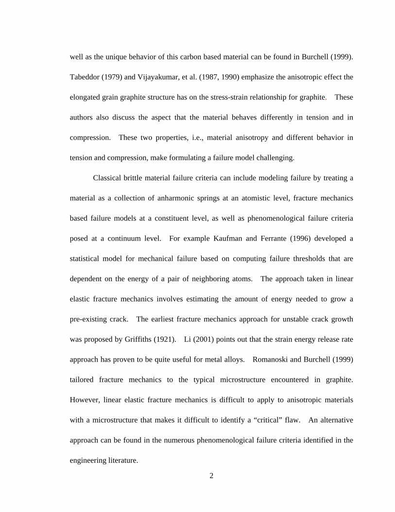
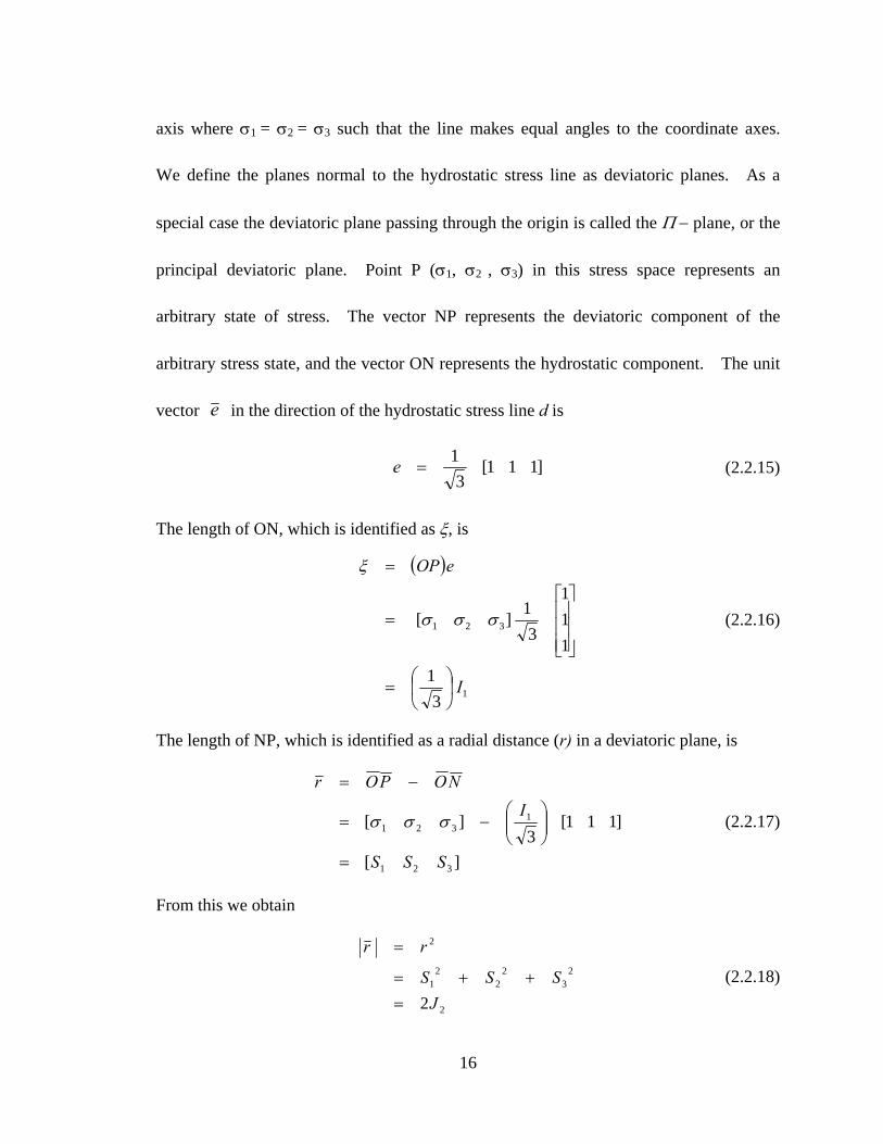
Figure 2.3.1 Decomposition of Stress in the Haigh-Westergaard (Principal) Stress Space
2.3 Graphical Representation of Stress
The reader is directed to Boresi and Schmidt (2003) for a comprehensive
discussion on the graphical representation of models in various stress spaces. In the
Haigh-Westergaard stress space a given stress state (1, 2, 3) can be graphically
decomposed into hydrostatic and deviatoric components. This decomposition is
depicted graphically in Figure 2.3.1. Line d in figure 2.3.1 represents the hydrostatic
N
1
2
3
O
d
),,( 321 P
rComponentDevatoric
ComponentcHydrostati
16
axis where 1 = 2 = 3 such that the line makes equal angles to the coordinate axes.
We define the planes normal to the hydrostatic stress line as deviatoric planes. As a
special case the deviatoric plane passing through the origin is called the plane, or the
principal deviatoric plane. Point P (1, 2 , 3) in this stress space represents an
arbitrary state of stress. The vector NP represents the deviatoric component of the
arbitrary stress state, and the vector ON represents the hydrostatic component. The unit
vector e in the direction of the hydrostatic stress line d is
]111[3
1e (2.2.15)
The length of ON, which is identified as , is
1
321
3
1
1
1
1
3
1][
I
eOP
(2.2.16)
The length of NP, which is identified as a radial distance (r) in a deviatoric plane, is
][
]111[3
][
321
1321
SSS
I
NOPOr
(2.2.17)
From this we obtain
2
23
22
21
2
2J
SSS
rr
(2.2.18)
17
such that
22Jr (2.2.19)
One more relationship between invariants is presented. An angle, identified in
the literature as Lode’s angle, can be defined on the deviatoric plane. This angle is
formed from the projection of the 1 – axis onto a deviatoric plane and the radius vector
in the deviatoric plane, r . The magnitude of the angle is computed from the
expression
)600()(2
33cos
3
1 0023
2
31
J
J (2.2.20)
As the reader will see this relationship will be used to develop failure criterion. It is also
used here to plot failure data.
We now have several graphical schemes to present functions that are defined by
various failure criteria. They are
a principal stress plane (e.g., the 1 - 2 plane);
the use of a deviatoric plane presented in the Haigh-Westergaard stress
space; or
meridians along failure surfaces presented in the Haigh-Westergaard stress
space that are projected onto a plane defined by the coordinate axes
( r ).
18
Each presentation method will be utilized in turn to highlight aspects of the failure
criteria discussed herein. We begin with one parameter phenomenological models and
then discuss progressively more complex models in later chapters.
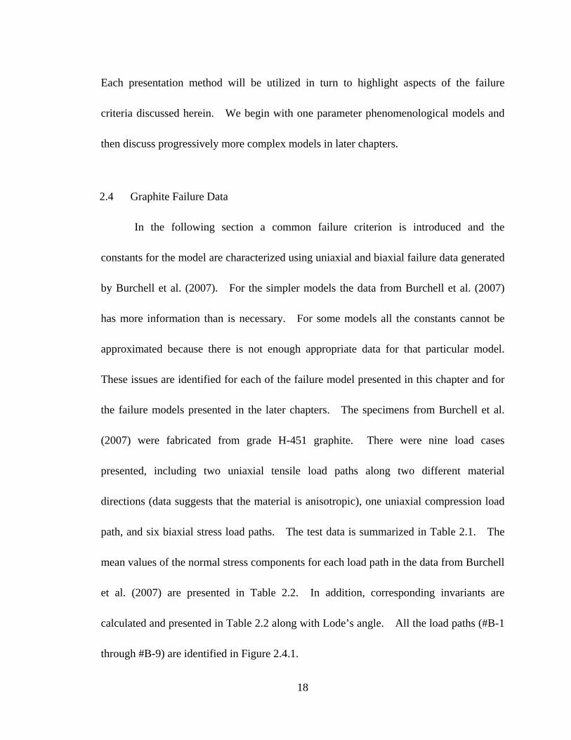
2.4 Graphite Failure Data
In the following section a common failure criterion is introduced and the
constants for the model are characterized using uniaxial and biaxial failure data generated
by Burchell et al. (2007). For the simpler models the data from Burchell et al. (2007)
has more information than is necessary. For some models all the constants cannot be
approximated because there is not enough appropriate data for that particular model.
These issues are identified for each of the failure model presented in this chapter and for
the failure models presented in the later chapters. The specimens from Burchell et al.
(2007) were fabricated from grade H-451 graphite. There were nine load cases
presented, including two uniaxial tensile load paths along two different material
directions (data suggests that the material is anisotropic), one uniaxial compression load
path, and six biaxial stress load paths. The test data is summarized in Table 2.1. The
mean values of the normal stress components for each load path in the data from Burchell
et al. (2007) are presented in Table 2.2. In addition, corresponding invariants are
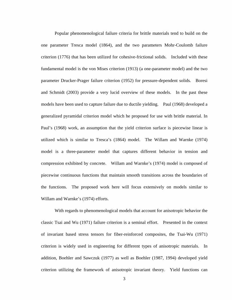
calculated and presented in Table 2.2 along with Lode’s angle. All the load paths (#B-1
through #B-9) are identified in Figure 2.4.1.
19
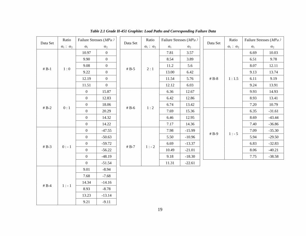
Table 2.1 Grade H-451 Graphite: Load Paths and Corresponding Failure Data
Data Set Ratio
Failure Stresses (MPa)
# B-1 1 : 0
10.97 0
9.90 0
9.08 0
9.22 0
12.19 0
11.51 0
# B-2 0 : 1
0 15.87
0 12.83
0 18.06
0 20.29
0 14.32
0 14.22
# B-3 0 : - 1
0 -47.55
0 -50.63
0 -59.72
0 -56.22
0 -48.19
0 -51.54
# B-4 1 : - 1
9.01 -8.94
7.68 -7.68
14.34 -14.16
8.93 -8.78
13.23 -13.14
9.21 -9.11
Data Set Ratio
Failure Stresses (MPa)
# B-5 2 : 1
7.81 3.57
8.54 3.89
11.2 5.6
13.00 6.42
11.54 5.76
12.12 6.03
# B-6 1 : 2
6.36 12.67
6.42 12.86
6.74 13.42
7.69 15.36
6.46 12.95
7.17 14.36
# B-7 1 : - 2
7.98 -15.99
5.50 -10.96
6.69 -13.37
10.49 -21.01
9.18 -18.30
11.31 -22.61
Data Set Ratio
Failure Stresses (MPa)
# B-8 1 : 1.5
6.69 10.03
6.51 9.78
8.07 12.11
9.13 13.74
6.11 9.19
9.24 13.91
9.93 14.93
8.93 13.41
7.20 10.79
# B-9 1 : - 5
6.35 -31.61
8.69 -43.44
7.40 -36.86
7.09 -35.30
5.94 -29.50
6.83 -32.83
8.06 -40.21
7.75 -38.58

20
Figure 2.4.1 Load Paths from Burchell et al. (2007) Plotted in a 1 – 2 Stress Space
Table 2.2 Invariants of the Average Failure Strengths for All 9 Load Paths
Data Set (1)ave (MPa) (2)ave (MPa) (MPa) r (MPa)
# B-1 10.48 0 6.05 8.56 0.00o
# B-2 0 15.93 9.20 13.01 0.00 o
# B-3 0 -52.93 -30.56 43.22 60.00 o
# B-4 10.4 -10.3 0.06 14.64 29.84 o
# B-5 10.7 5.21 9.19 7.57 29.13 o
# B-6 6.81 13.6 11.78 9.62 30.05o
# B-7 8.53 -17.04 -4.91 18.41 40.88 o
# B-8 7.98 11.99 11.53 8.63 40.82 o
# B-9 7.26 -36.04 -16.62 32.79 50.99 o
21
1x
2x
3x
T
T
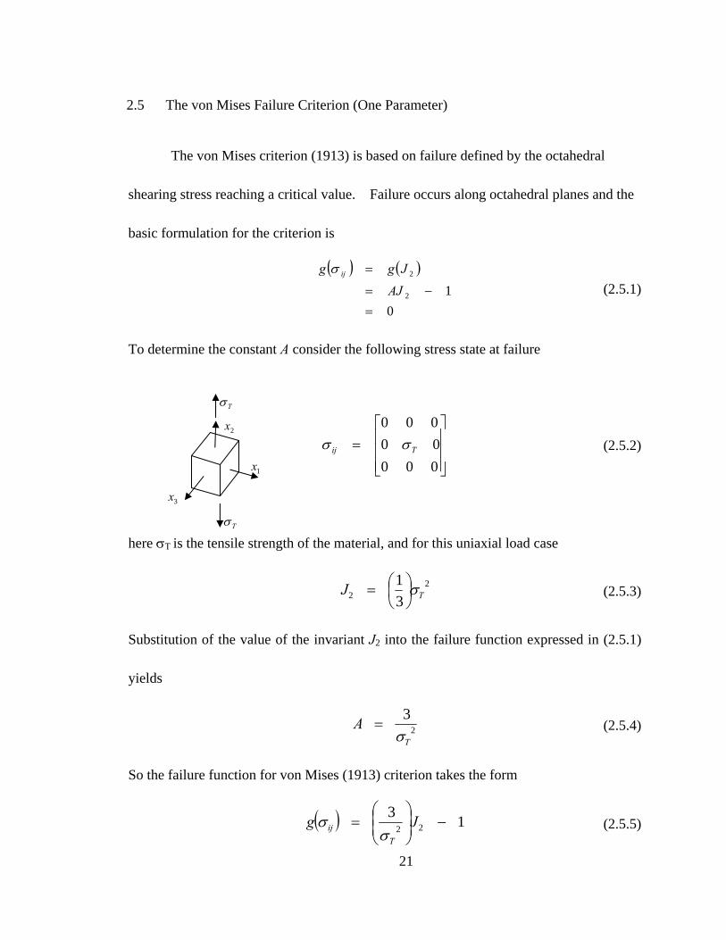
2.5 The von Mises Failure Criterion (One Parameter)
The von Mises criterion (1913) is based on failure defined by the octahedral
shearing stress reaching a critical value. Failure occurs along octahedral planes and the
basic formulation for the criterion is
0
12
2
AJ
Jgg ij (2.5.1)
To determine the constant A consider the following stress state at failure
0 0 0
0 0
0 0 0
Tij (2.5.2)
here is the tensile strength of the material, and for this uniaxial load case
2
2 3
1TJ
(2.5.3)
Substitution of the value of the invariant J2 into the failure function expressed in (2.5.1)
yields
2
3
T
A
(2.5.4)
So the failure function for von Mises (1913) criterion takes the form
13
22
Jg
T
ij (2.5.5)
22
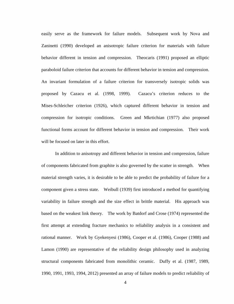
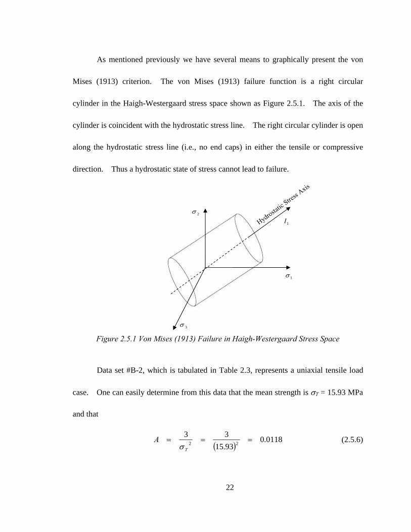
As mentioned previously we have several means to graphically present the von
Mises (1913) criterion. The von Mises (1913) failure function is a right circular
cylinder in the Haigh-Westergaard stress space shown as Figure 2.5.1. The axis of the
cylinder is coincident with the hydrostatic stress line. The right circular cylinder is open
along the hydrostatic stress line (i.e., no end caps) in either the tensile or compressive
direction. Thus a hydrostatic state of stress cannot lead to failure.
Figure 2.5.1 Von Mises (1913) Failure in Haigh-Westergaard Stress Space
Data set #B-2, which is tabulated in Table 2.3, represents a uniaxial tensile load
case. One can easily determine from this data that the mean strength is T = 15.93 MPa
and that
0118.093.15
3322
T
A
(2.5.6)
1
1I2
3
23
For a uniaxial load path where the stress is equal to the mean strength value for T , the
components of this stress state in the Haigh-Westergaard stress space are
MPa
MPar
20.9
01.13
(2.5.7)
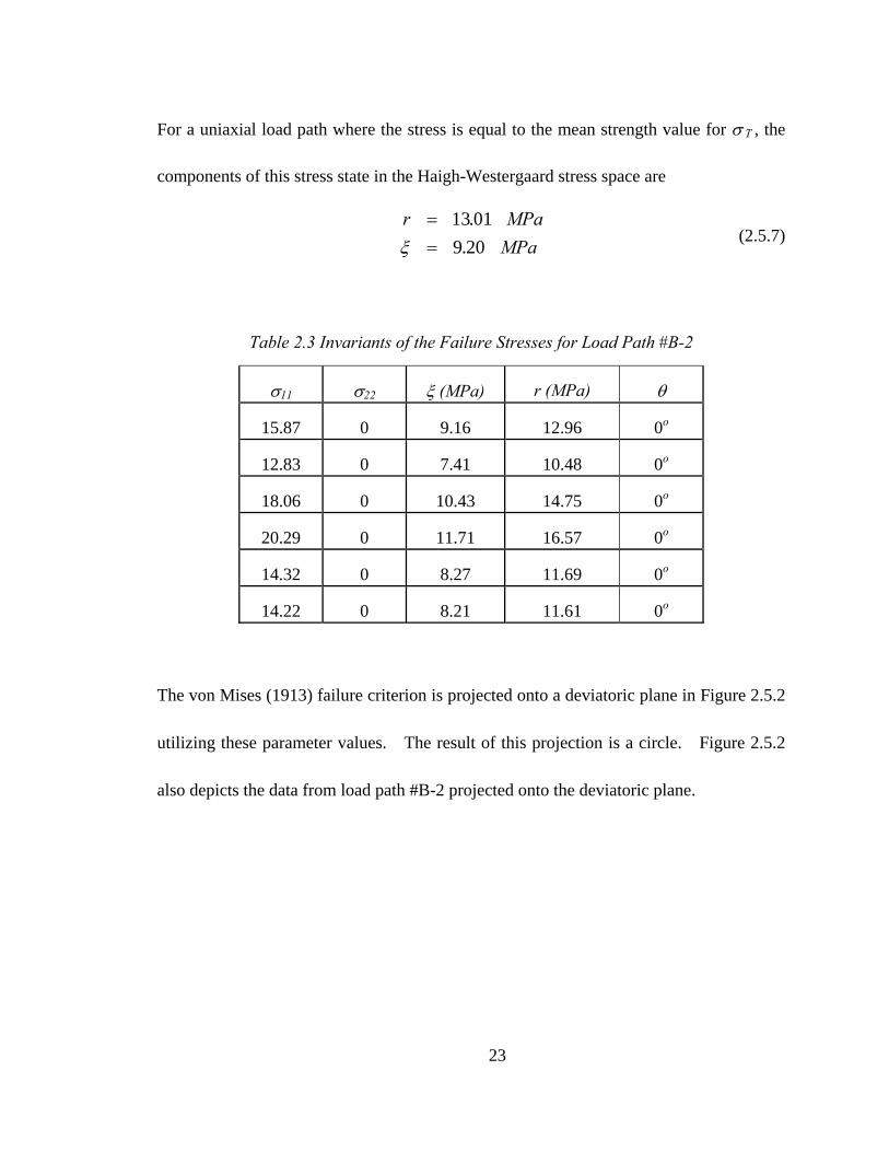
Table 2.3 Invariants of the Failure Stresses for Load Path #B-2
11 22 (MPa) r (MPa)
15.87 0 9.16 12.96 0o
12.83 0 7.41 10.48 0o
18.06 0 10.43 14.75 0o
20.29 0 11.71 16.57 0o
14.32 0 8.27 11.69 0o
14.22 0 8.21 11.61 0o
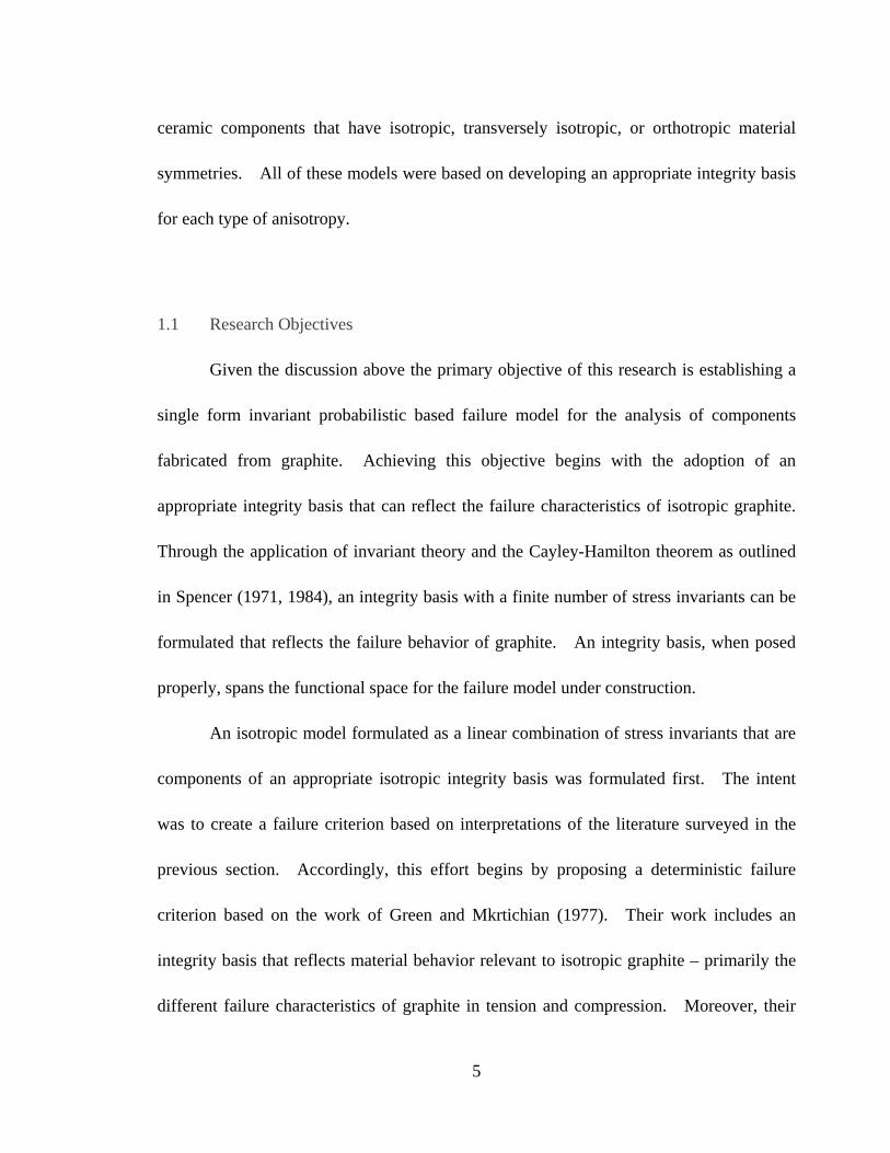
The von Mises (1913) failure criterion is projected onto a deviatoric plane in Figure 2.5.2
utilizing these parameter values. The result of this projection is a circle. Figure 2.5.2
also depicts the data from load path #B-2 projected onto the deviatoric plane.

24
Figure 2.5.2 The Von Mises (1913) Criterion Is Projected onto a Deviatoric Plane MPa20.9 Parallel to the Deviatoric Plan with T = 15.93 MPa
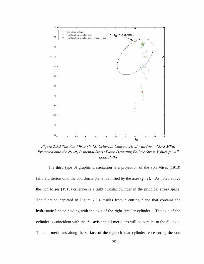
The von Mises (1913) failure criterion is also projected onto a 1 - 2 stress plane
in Figure 2.5.3. A right circular cylinder projected onto this plane presents as an ellipse.
An aspect of the von Mises (1913) failure model is that tensile and compressive failure
strengths are equal which is clearly evident in Figure 2.5.3. Obviously the data from
Burchell et al. (2007), which is also depicted in Figure 2.5.3, strongly suggests that
tensile strength is not equal to the compressive strength for this graphite material.
25
Figure 2.5.3 The Von Mises (1913) Criterion Characterized with (T = 15.93 MPa)
Projected onto the 1 -2 Principal Stress Plane Depicting Failure Stress Values for All Load Paths
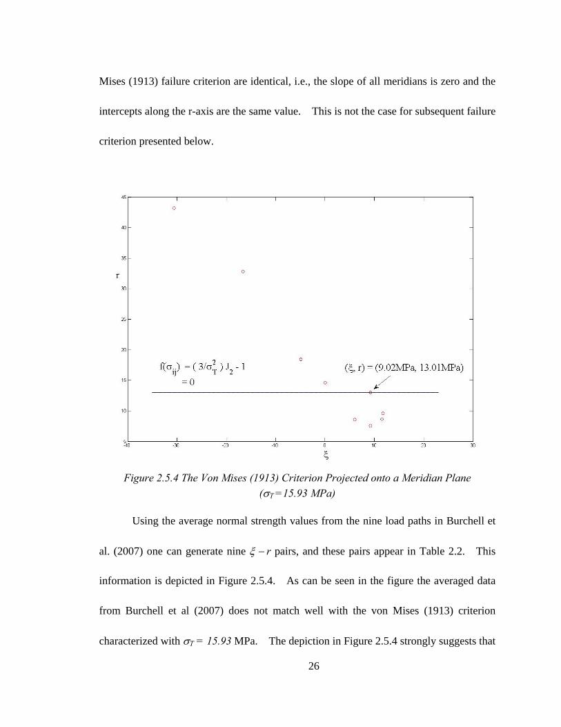
The third type of graphic presentation is a projection of the von Mises (1913)
failure criterion onto the coordinate plane identified by the axes (- r). As noted above
the von Mises (1913) criterion is a right circular cylinder in the principal stress space.
The function depicted in Figure 2.5.4 results from a cutting plane that contains the
hydrostatic line coinciding with the axis of the right circular cylinder. The axis of the
cylinder is coincident with the – axis and all meridians will be parallel to the – axis.
Thus all meridians along the surface of the right circular cylinder representing the von
26
Mises (1913) failure criterion are identical, i.e., the slope of all meridians is zero and the
intercepts along the r-axis are the same value. This is not the case for subsequent failure
criterion presented below.
Figure 2.5.4 The Von Mises (1913) Criterion Projected onto a Meridian Plane
(T =15.93 MPa)
Using the average normal strength values from the nine load paths in Burchell et
al. (2007) one can generate nine r pairs, and these pairs appear in Table 2.2. This
information is depicted in Figure 2.5.4. As can be seen in the figure the averaged data
from Burchell et al (2007) does not match well with the von Mises (1913) criterion
characterized with T = 15.93 MPa. The depiction in Figure 2.5.4 strongly suggests that
27
, or I1, should be considered in developing the failure function, i.e., something more than
the J2 should be used to construct the model. Since nuclear graphite is not fully dense,
we will assume that the hydrostatic component of the stress state contributes to failure.
In addition, the von Mises (1913) criterion does not allow different strength in tension
and compression. When other formulations are considered in the next chapter their
dependence will have a well-defined dependence on I1. This invariant will permit
different strengths in tension and compression, e.g., the classic the Drucker–Prager
(1952) failure criterion outlined in the next section.
As a final note on the one parameter models, the Tresca criterion (1864) could
have been considered here. Although based on the concept that failure occurs when a
maximum shear strength of a material is attained, this model is a piecewise continuous
failure criterion. Although later criterion considered here are similarly piecewise
continuous, the Tresca (1864) failure criterion does not mandate continuous slopes at the
boundaries of various regions of the stress space. This condition will be imposed on the
failure criterion considered later.
28
CHAPTER III
TWO AND THREE PARAMETER FAILURE CRITERIA
In the previous chapter failure data from Burchell et al. (2007) was presented in
terms of a familiar one parameter failure criterion, i.e., the von Mises (1913) criterion.
The von Mises (1913) failure criterion can be characterized through a single strength
parameter – the shear strength on the octahedral stress plane. In this chapter the view is
expanded and details of two and three parameter failure criterion are presented in terms
of how well the criterion perform relative to the mean strength of various load paths from
Burchell et al. (2007).
3.1 The Drucker-Prager Failure Criterion (Two Parameter)
In this section we consider an extension of the Von Mises (1913) criterion, i.e., a
failure model that includes the I1 invariant. This extension is the Drucker – Prager
(1952) criterion and is defined by the failure function
0
1, 2121
JBAIJIg (3.1.1)
29
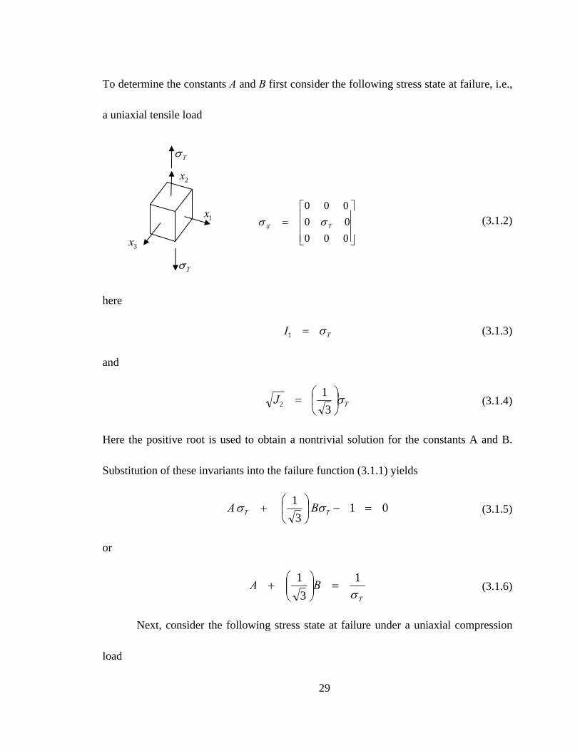
To determine the constants A and B first consider the following stress state at failure, i.e.,
a uniaxial tensile load
0 0 0
0 0
0 0 0
Tij (3.1.2)
here
TI 1 (3.1.3)
and
TJ
3
12 (3.1.4)
Here the positive root is used to obtain a nontrivial solution for the constants A and B.
Substitution of these invariants into the failure function (3.1.1) yields
013
1
TT BA (3.1.5)
or
T
BA1
3
1
(3.1.6)
Next, consider the following stress state at failure under a uniaxial compression
load
1x
2x
3x
T
T

30
000
00
000
Cij (3.1.7)
where
CI 1 (3.1.8)
and
CJ
3
12 (3.1.9)
where the negative root is used here to obtain a nontrivial solution for the constants A and
B. Substitution of these invariants into the failure function (3.1.1) yields
013
1
CC BA (3.1.10)
or
C
BA1
3
1
(3.1.11)
Simultaneous solution of equations (3.1.6) and (3.1.11) yields
CT
A11
2
1 (3.1.12)
CT
B11
2
3 (3.1.13)
1x
2x
3x
C
C
31
Using the data from load path #B-2 in Burchell et al. (2007) the average tensile strength
is
MPaT 93.15 (3.1.14)
In a similar manner, using the load path #B-3, the average compressive strength is
MPaC 93.52 (3.1.15)
With these values of T and C the parameters A and B are
102194.0
93.52
1
93.15
1
2
1
MPa
A (3.1.16)
and
107073.0
93.52
1
93.15
1
2
3
MPa
B (3.1.17)
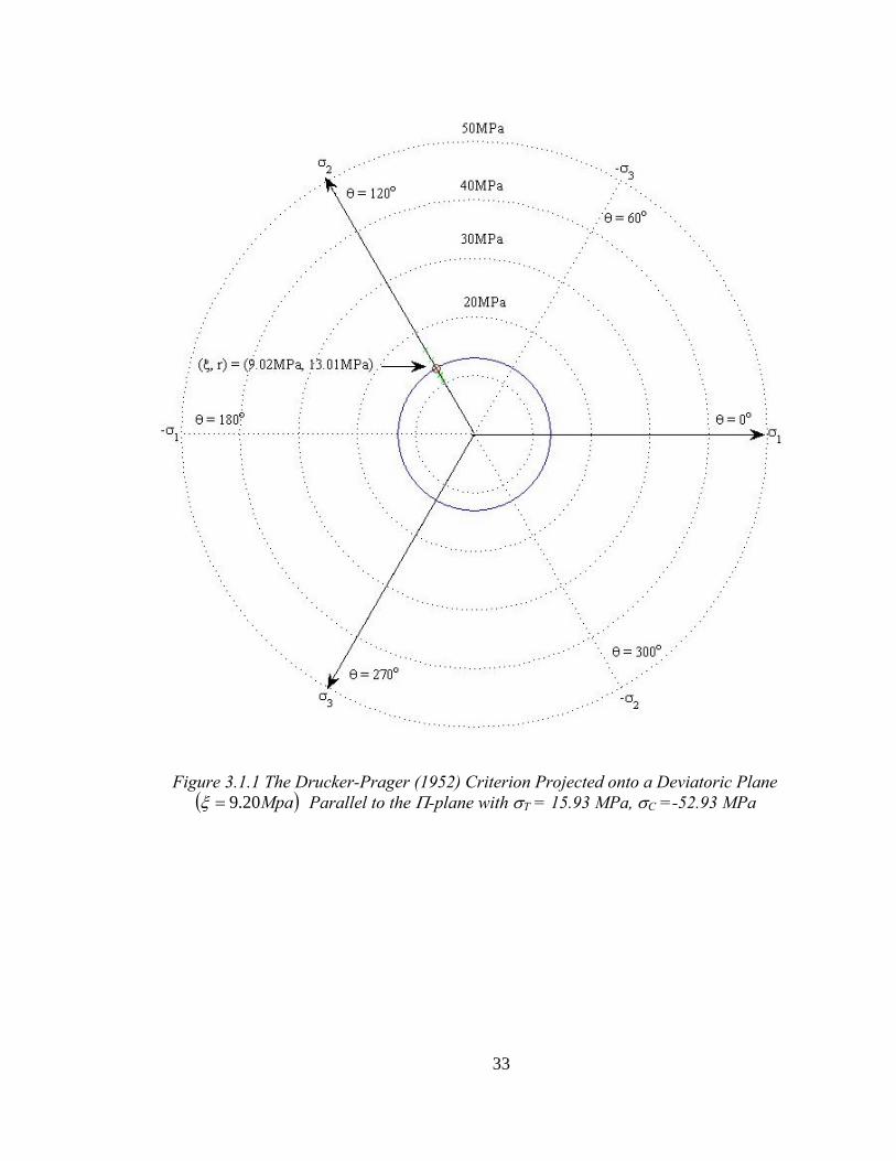
The Drucker-Prager (1952) failure criterion is first projected onto the deviatoric
plane defined by
MPa20.9 (3.1.18)
in Figure 3.1.1. There are an infinite number of deviatoric planes parallel to the -
plane. For the Drucker-Prager (1952) failure criterion each projection will represent a
circle with a different diameter on a different deviatoric plane. In addition, the graphical
depiction of the Drucker-Prager (1952) failure criterion projected onto the deviatoric
plane defined by
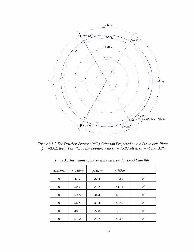
MPa2.30 (3.1.19)
32
is depicted in Figure 3.1.2. This value of is obtained from averaging the compressive
strength data along load path #B-3. The invariants associated with a strength averaged
from all the load data along path #B-3 are listed in Table 2.2. The invariants for
individual failure strengths along load path #B-3 are presented in Table 3.1 and the
failure data along load path #B-3 are also depicted in Figure 3.1.2. The Drucker-Prager
(1952) failure criterion can be thought of as a right circular cone with the tip of the cone
located along the positive – axis. The cone opens up along the – axis as becomes
more and more negative. The negative value of from equation 3.1.19 denotes a
deviatoric plane beyond the - plane where = 0. The failure criterion depicted in
Figure 3.1.2 has a larger diameter than the failure criterion depicted in Figure 3.1.1.
33
Figure 3.1.1 The Drucker-Prager (1952) Criterion Projected onto a Deviatoric Plane Mpa20.9 Parallel to the -plane with T = 15.93 MPa, C =-52.93 MPa
34
Figure 3.1.2 The Drucker-Prager (1952) Criterion Projected onto a Deviatoric Plane Mpa2.30 Parallel to the -plane with T = 15.93 MPa, C = -52.93 MPa
Table 3.1 Invariants of the Failure Stresses for Load Path #B-3
11(MPa) 22(MPa) (MPa) r (MPa)
0 -47.55 -27.45 38.82 0o
0 -50.63 -29.23 41.34 0o
0 -59.72 -34.48 48.76 0o
0 -56.22 -32.46 45.90 0o
0 -48.19 -27.82 39.35 0o
0 -51.54 -29.76 42.08 0o

35
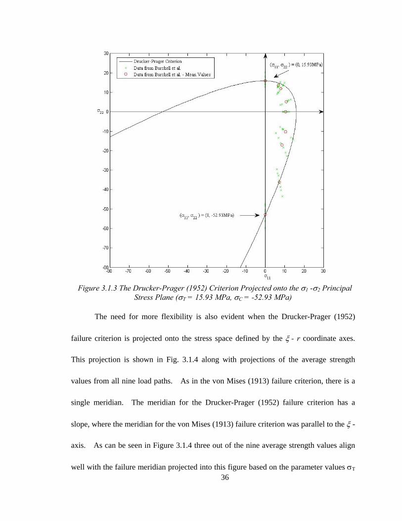
In Figure 3.1.3 the failure criterion is projected onto the 1 -2 stress plane along
and is compared with all the data from Burchell et al. (2007). The right circular cone
typically projects as an elongated ellipse in this stress space. The Drucker-Prager
(1952) failure criterion matches the mean failure stress along the 1 - tensile load path
(load path #B-2) and the 1 – compressive load path (load path #B-3), as it should since
the criterion was characterized with the data along these two load paths. However the
criterion does not match the data along the 2 tensile load path (load path #B-1). The
H-451 graphite that Burchell et al. (2007) tested is slightly anisotropic. Moreover, the
failure data from the biaxial stress load paths, #B-4 through #B-8 do not match well with
the criterion characterized using tensile and compressive strength data. The exception
to this is along load path #B-9. This indicates a need for more flexibility from the
failure model in order to phenomenologically capture the biaxial failure data.
36
Figure 3.1.3 The Drucker-Prager (1952) Criterion Projected onto the 1 -2 Principal Stress Plane (T = 15.93 MPa, C = -52.93 MPa)
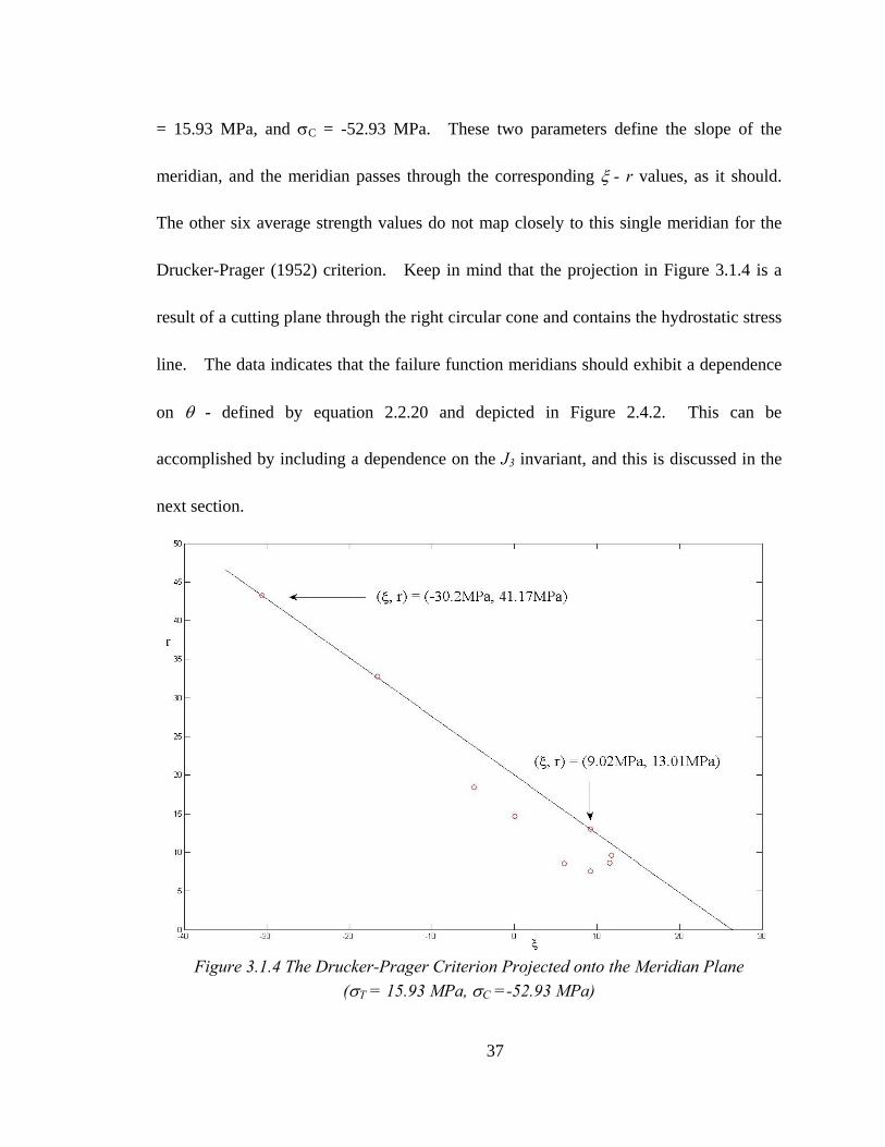
The need for more flexibility is also evident when the Drucker-Prager (1952)
failure criterion is projected onto the stress space defined by the - r coordinate axes.
This projection is shown in Fig. 3.1.4 along with projections of the average strength
values from all nine load paths. As in the von Mises (1913) failure criterion, there is a
single meridian. The meridian for the Drucker-Prager (1952) failure criterion has a
slope, where the meridian for the von Mises (1913) failure criterion was parallel to the -
axis. As can be seen in Figure 3.1.4 three out of the nine average strength values align
well with the failure meridian projected into this figure based on the parameter values T
37
= 15.93 MPa, and C = -52.93 MPa. These two parameters define the slope of the
meridian, and the meridian passes through the corresponding - r values, as it should.
The other six average strength values do not map closely to this single meridian for the
Drucker-Prager (1952) criterion. Keep in mind that the projection in Figure 3.1.4 is a
result of a cutting plane through the right circular cone and contains the hydrostatic stress
line. The data indicates that the failure function meridians should exhibit a dependence
on - defined by equation 2.2.20 and depicted in Figure 2.4.2. This can be
accomplished by including a dependence on the J3 invariant, and this is discussed in the
next section.
Figure 3.1.4 The Drucker-Prager Criterion Projected onto the Meridian Plane
(T = 15.93 MPa, C =-52.93 MPa)

38
As noted above and depicted in Figure 3.1.3 the Drucker-Prager failure curve is
open along the equal biaxial compression load path. The following derivation will
demonstrate the transition from a parabolic (open) curve to an elliptic (closed) curve is
based on the strength ratio C T. Consider the equal biaxial compression stress state
with BC < 0
000
00
00
BC
BC
ij (3.1.20)
The corresponding deviatoric stress tensor is
3
200
03
0
003
BC
BC
BC
ij
σ
σ
σ
S (3.1.21)
The stress invariants of this state of stress are
BCI 21 (3.1.22)
and
BCJ
3
12 (3.1.23)
Substitution of these invariants into the failure function (3.1.1) yields
013
1)2(
BCBC BA (3.1.24)
or
39
BABC
3
12
1 (3.1.25)
Since BC < 0, then
0
3
12
1
BA
BC (3.1.26)
which infers
BA
3
12 (3.1.27)
This leads to
CTCT 11
2
3
3
111
2
12 (3.1.28)
or
CT
31 (3.1.29)
Thus
3T
C
(3.1.30)
When the ratio of compressive strength and tensile strength (C T) < 3, the
Drucker-Prager failure criterion projects an elliptical (closed) curve in the 1 -2 stress
plane.
Consider the following biaxial state of stress
40
000
00
00
y
x
ij
(3.1.31)
The corresponding deviatoric stress tensor is
300
03
20
003
2
yx
xy
yx
ijS
(3.1.33)
The stress invariants for this state of stress are
yxI 1 (3.1.32)
and
222 3
1yyxxJ
(3.1.34)
Substitution of these invariants into equation (3.1.1) yields
0
13
1
,
22
21
yyxx
yx
B
AJIf
(3.1.35)
or
B
A yxyyxx
1
3
1 22 (3.1.36)
Squaring both sides yields
0366
)6()3()3( 22222
yx
yxyx
AA
BAABAB
(3.1.37)
41
The shape of the failure criterion defined by equation (3.1.37) is determined by the values
of the two parameters A and B. Using tensile data from Burchell et al. (2007) where T
= 15.93 MPa and a ratio of compressive strength to tensile strength of (C T) = 2, then
C = -31.86 MPa and the parameters A and B are
101569.0
86.31
1
93.15
1
2
1
MPa
A (3.1.38)
and
108155.0
86.31
1
93.15
1
2
3
MPa
B (3.1.39 )
Equation (3.1.37) becomes
30942.00942.0
0081.00059.00059.0 22
yx
yxyx
(3.1.40 )
This expression is plotted in the 11 – 22 stress plane depicted in Figure 3.1.5
42
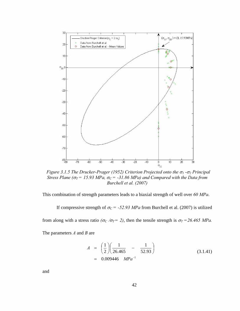
Figure 3.1.5 The Drucker-Prager (1952) Criterion Projected onto the 1 -2 Principal Stress Plane (T = 15.93 MPa, C = -31.86 MPa) and Compared with the Data from
Burchell et al. (2007)
This combination of strength parameters leads to a biaxial strength of well over 60 MPa.
If compressive strength of C = -52.93 MPa from Burchell et al. (2007) is utilized
from along with a stress ratio (C T = 2), then the tensile strength is T =26.465 MPa.
The parameters A and B are
1009446.0
93.52
1
465.26
1
2
1
MPa
A (3.1.41)
and
43
10490855.0
93.52
1
465.26
1
2
3
MPa
B (3.1.42)
Now
30567.00567.0
0029.00021.00021.0 22
yx
yxyx
(3.1.44)
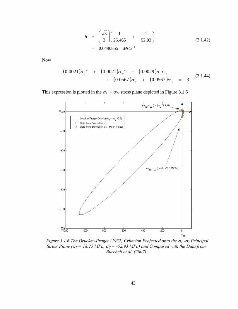
This expression is plotted in the 11 – 22 stress plane depicted in Figure 3.1.6
Figure 3.1.6 The Drucker-Prager (1952) Criterion Projected onto the 1 -2 Principal Stress Plane (T = 18.25 MPa, C = -52.93 MPa) and Compared with the Data from
Burchell et al. (2007)
44
Here the biaxial compressive strength is somewhat less than 1,100 MPa. In both
figures, i.e., Figure 3.1.5 and 3.1.6, closed ellipses are obtained which are important since
all load paths in this stress space eventually lead to failure. In Figure 3.1.3 the equal
biaxial compression load path was not bounded by the failure criterion given the strength
parameters extracted from the data from Burchell et al. (2007). For all failure criteria
considered, only those with closed failure surfaces are relevant for consideration.
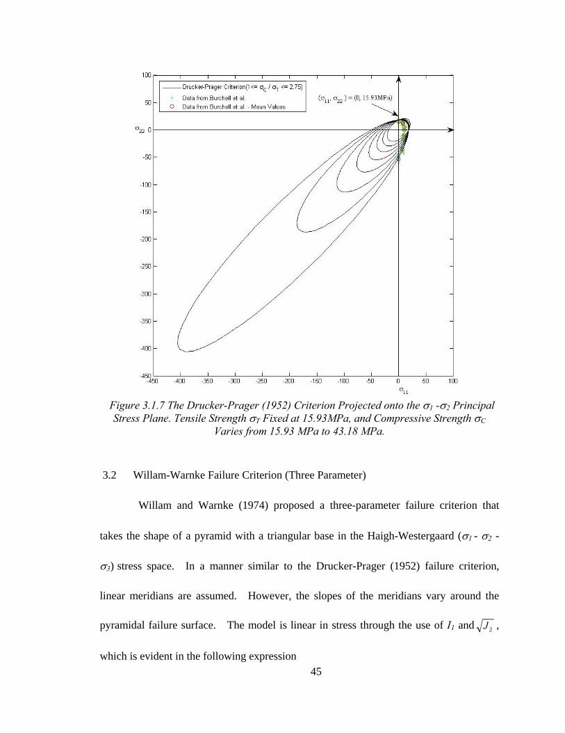
In order to see the full effect of the ratio of compression to tension strengths, this
ratio is varied from a value of 1.0 to 2.75 in increments of 0.25 in Figure 3.1.7. The
ratio was computed by holding T fixed at the mean value of the data from Burchell et al.
(2007) for load path B-2, i.e., 15.93 MPa, and increasing the strength parameter C from
15.93 MPa to 2.75 times this value, i.e., 43.81 MPa.
45
Figure 3.1.7 The Drucker-Prager (1952) Criterion Projected onto the 1 -2 Principal Stress Plane. Tensile Strength T Fixed at 15.93MPa, and Compressive Strength C
Varies from 15.93 MPa to 43.18 MPa.
3.2 Willam-Warnke Failure Criterion (Three Parameter)
Willam and Warnke (1974) proposed a three-parameter failure criterion that
takes the shape of a pyramid with a triangular base in the Haigh-Westergaard (1 - 2 -
3) stress space. In a manner similar to the Drucker-Prager (1952) failure criterion,
linear meridians are assumed. However, the slopes of the meridians vary around the
pyramidal failure surface. The model is linear in stress through the use of I1 and 2J ,
which is evident in the following expression
46
0
1),(,, 2321321
JJJBAIJJIg (3.2.1)
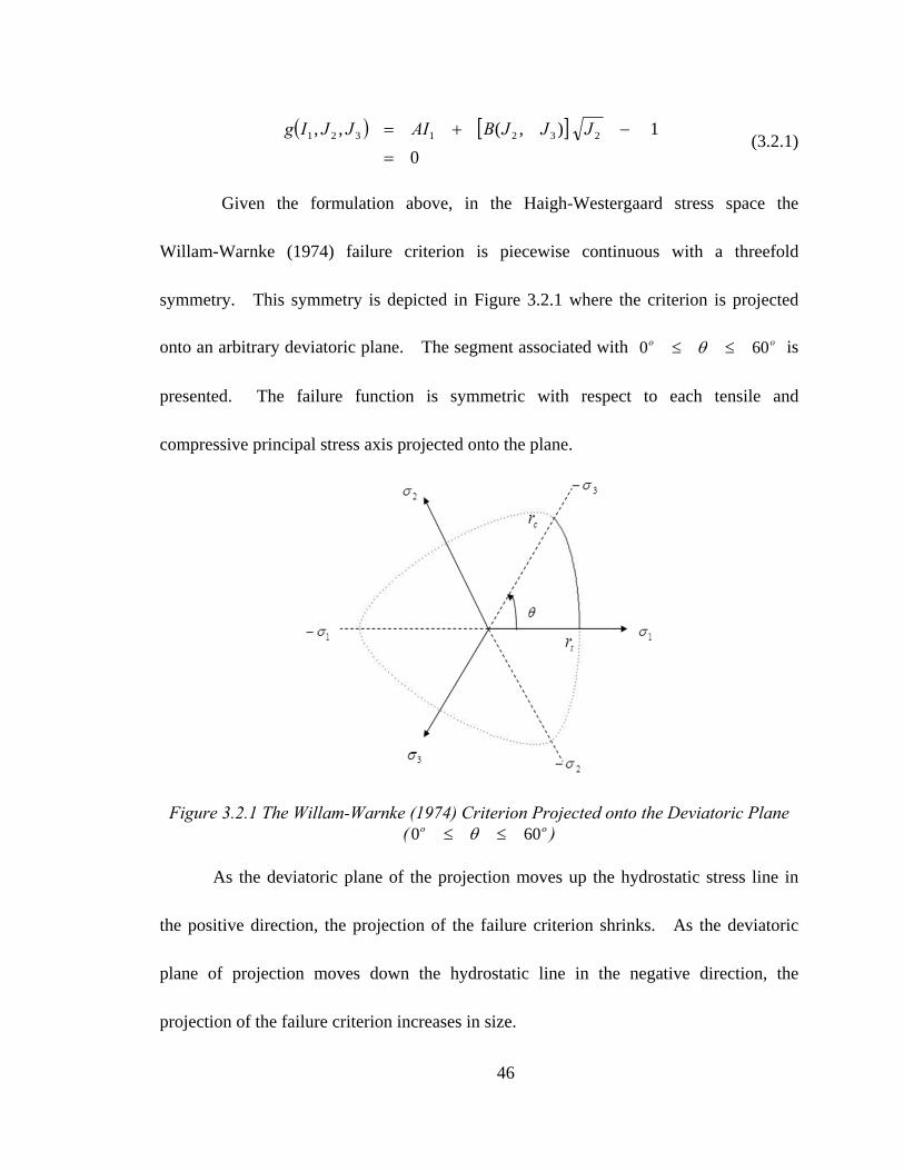
Given the formulation above, in the Haigh-Westergaard stress space the
Willam-Warnke (1974) failure criterion is piecewise continuous with a threefold
symmetry. This symmetry is depicted in Figure 3.2.1 where the criterion is projected
onto an arbitrary deviatoric plane. The segment associated with oo 600 is
presented. The failure function is symmetric with respect to each tensile and
compressive principal stress axis projected onto the plane.
Figure 3.2.1 The Willam-Warnke (1974) Criterion Projected onto the Deviatoric Plane ( oo 600 )
As the deviatoric plane of the projection moves up the hydrostatic stress line in
the positive direction, the projection of the failure criterion shrinks. As the deviatoric
plane of projection moves down the hydrostatic line in the negative direction, the
projection of the failure criterion increases in size.
47
Willam and Warnke (1974) defined the parameter B from equation 3.2.1 in the
following manner
)(
1
rB (3.2.2)
where r is a radial vector located in a plane parallel to the -plane. Willam and
Warnke (1974) assumed that when the failure surface was projected onto a deviatoric
plane that a segment of this projection could be defined as a segment of an elliptic curve
with the following formulation
2222
21222222
)2(cos)((4
]45cos)((4)[2(cos)(2
tctc
ctttcctctcc
rrrr
rrrrrrrrrrrr
(3.2.3)
Here is Lode’s angle, where once again
)600()(
)(
2
33cos
3
1 003
2
331
J
J (3.2.4)
When o0 , TBB , Trr and
T
T Br
1 (3.2.5)
Similarly, with o60 , CBB , Crr and
C
C Br
1 (3.2.6)
In order to determine the constants BT and BC consider the following stress state
48
0 0 0
0 0
0 0 0
Tij (3.2.7)
The deviatoric stress tensor is
TijS
3
1 0 0
0 3
2 0
0 0 3
1
(3.2.8)
and Lode’s angle as wells as the three invariants obtained are expressed as
TTTJJI
3
2,
3
3,,,
33
321 (3.2.9)
)600(0 000 (3.2.10)
Substitution of the values of invariants into failure function given by equation (3.2.1)
yields
01)(3
3)(
TTT BA (3.2.11)
or
T
TBA1
3
3
(3.2.12)
1x
2x
3x
C
C

49
Next consider a uniaxial compressive stress state characterized by the following
stress tensor.
000
00
000
Cij (3.2.13)
then
c
3
1- 0 0
0 3
2 0
0 0 3
1
ijS (3.2.14)
and
C
3
CC3
321 3
2,
3
3,,, JJI (3.2.15)
060 (3.2.16)
Substitution of these the values for the invariants into the Willam-Warnke (1974) failure
function yields
01)(3
3CC
CBA (3.2.17)
C
1
3
3
CBA (3.2.18)
1x
2x
3x
C
C

50
At this point we have two equations (3.2.12 and 3.2.18) and three unknowns (A,
BT, and BC). In order to obtain a third equation consider an equal biaxial compressive
stress state characterized as
BC
BCij
00
00
000
(3.2.19)
Now the deviatoric stress tensor becomes
BC
3
1 0 0
0 3
1 0
0 0 3
2
ijS (3.2.20)
and
BC
3
BCBC3
321 3
2,
3
3,2,, JJI (3.2.21)
o0 (3.2.22)
Substitution of these invariants into failure function defined by equation (3.2.1) yields
013
32 BCBC
TBA (3.2.23)
or
1x
2x
3x
BC
BC
BCBC
51
BC
1
3
32
TBA (3.2.24)
We now have three equations, i.e., (3.2.12), (3.2.18) and (3.2.24), in three
unknowns A, Bt and Bc. Solution of this system of equations leads to the following three
expressions for the unknown model parameters
CT
11
3
1
A (3.2.25)
and
BCT
12
3
3
TB (3.2.26)
and
BCTC
11
3
113
CB (3.2.27)
In order to characterize to characterize the Willam and Warnke (1974) model in a
straight forward manner one would need failure data from a uniaxial load path, a uniaxial
compressive load path, and an equal biaxial compression load path. Unfortunately,
Burchell et al. (2007) did not conduct biaxial compression stress tests. It must be
pointed out that these tests are extremely difficult to perform. Here we arbitrarily
assume the magnitude of the biaxial compression stress at failure is 1.16 times the
uniaxial compression stress at failure. Thus the three sets of strength parameters
obtained from the data found in Burchell et al. (2007) are
T = 15.93 MPa (3.2.28)

52
for tension,
C = -52.93 MPa (3.2.29)
for compression and
BC = -61.40 MPa (3.2.30)
for the biaxial compression material strength. The important thing is that with the three
parameter Willam-Warnke (1974) criterion the biaxial compression strength is a direct
model input. Biaxial compression strength could be controlled indirectly in the
Drucker-Prager model (1952). The additional strength parameter in the Willam-Warnke
(1974) model brings additional flexibility and the criterion represents an increased
flexibility in modeling material behavior relative to the Drucker-Prager (1952) criterion
in a manner similar to a comparison of the Drucker-Prager (1952) model to the von Mises
(1913) model. However, the additional flexibility is not enough to capture the
anisotropic behavior exhibited by the graphite data from Burchell et al. (2007).
This is evident in Figure 3.2.2 where the Willam-Warnke (1974) criterion and all
of test data from Burchell et al. (2007) are projected onto the principal stress plane
defined by the 1 - 2 coordinate axes. The criterion seems to capture the biaxial failure
data along load path #B-8. However, there is an increasing loss of fidelity with load
paths #B-7 and #B-6. Load path #B-5 represents anisotropic strength behavior and the
Willam and Warnke (1974) model was constructed based on the assumption of an
isotropic material. The same behavior can be seen in biaxial load paths #B-4, #B-3 and
53
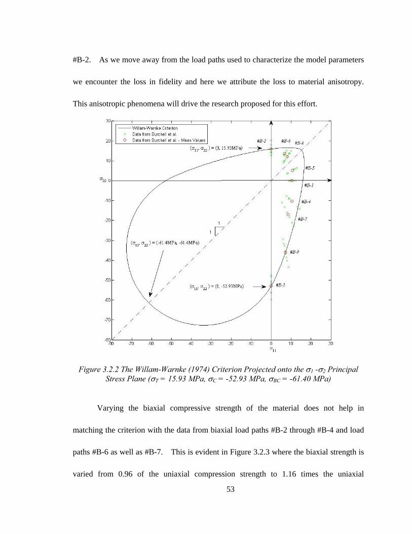
#B-2. As we move away from the load paths used to characterize the model parameters
we encounter the loss in fidelity and here we attribute the loss to material anisotropy.
This anisotropic phenomena will drive the research proposed for this effort.
Figure 3.2.2 The Willam-Warnke (1974) Criterion Projected onto the 1 -2 Principal Stress Plane (T = 15.93 MPa, C = -52.93 MPa, BC = -61.40 MPa)
Varying the biaxial compressive strength of the material does not help in
matching the criterion with the data from biaxial load paths #B-2 through #B-4 and load
paths #B-6 as well as #B-7. This is evident in Figure 3.2.3 where the biaxial strength is
varied from 0.96 of the uniaxial compression strength to 1.16 times the uniaxial
54
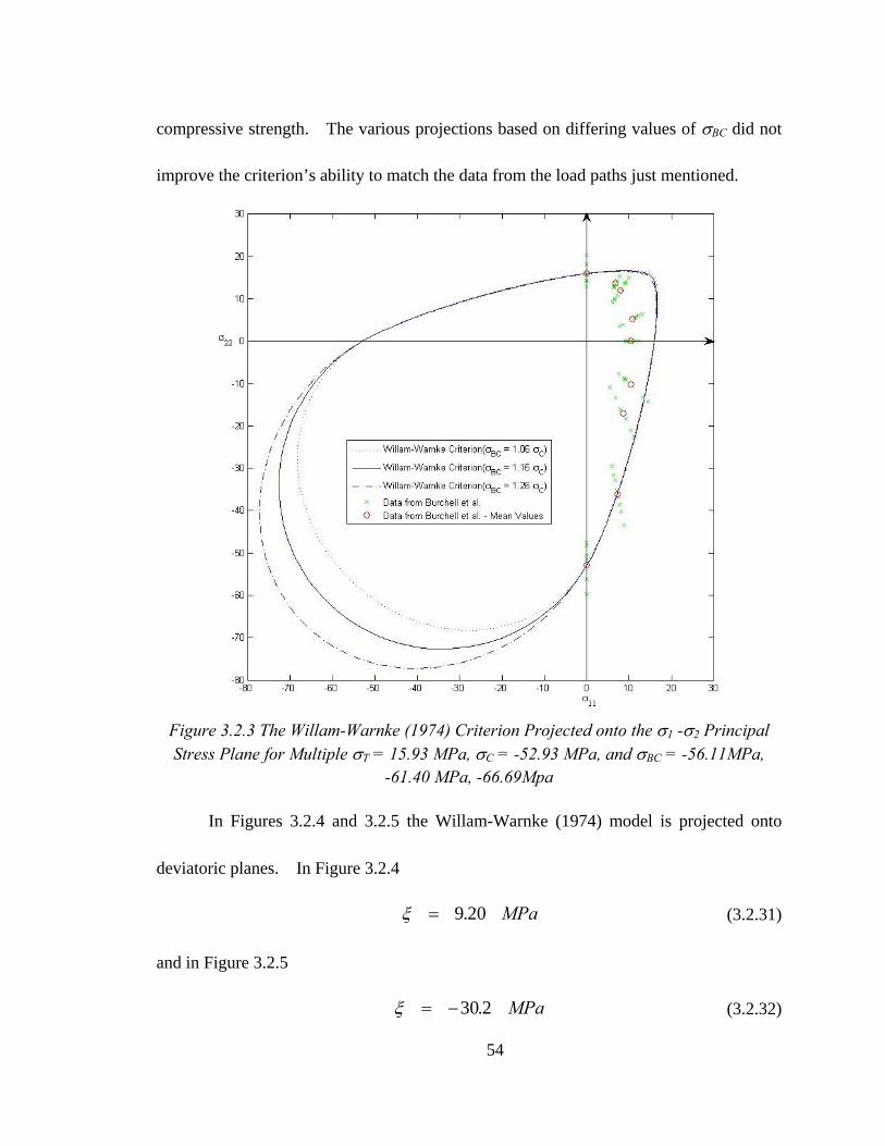
compressive strength. The various projections based on differing values of BC did not
improve the criterion’s ability to match the data from the load paths just mentioned.
Figure 3.2.3 The Willam-Warnke (1974) Criterion Projected onto the 1 -2 Principal Stress Plane for Multiple T = 15.93 MPa, C = -52.93 MPa, and BC = -56.11MPa,
-61.40 MPa, -66.69Mpa
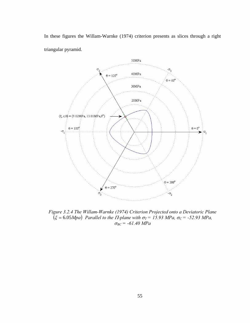
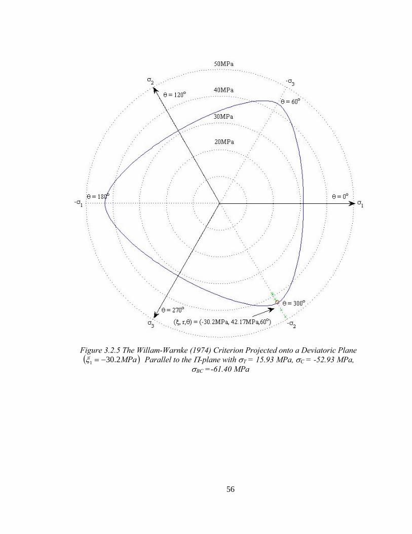
In Figures 3.2.4 and 3.2.5 the Willam-Warnke (1974) model is projected onto
deviatoric planes. In Figure 3.2.4
MPa20.9 (3.2.31)
and in Figure 3.2.5
MPa2.30 (3.2.32)
55
In these figures the Willam-Warnke (1974) criterion presents as slices through a right
triangular pyramid.
Figure 3.2.4 The Willam-Warnke (1974) Criterion Projected onto a Deviatoric Plane Mpa05.6 Parallel to the -plane with T = 15.93 MPa, C = -52.93 MPa,
BC = -61.40 MPa
56
Figure 3.2.5 The Willam-Warnke (1974) Criterion Projected onto a Deviatoric Plane MPa2.301 Parallel to the -plane with T = 15.93 MPa, C = -52.93 MPa,
BC =-61.40 MPa

57
Figure 3.2.6 The Willam-Warnke (1974) Criterion Projected onto the Meridian Plane for
a Material Strength Parameter of T = 15.93 MPa, C = -52.93 MPa, BC = -61.40 MPa
The meridian lines associated with the Willam-Warnke (1974) failure criterion for
Lode angle values of o0 and o60 are depicted on Figure 3.2.6. The meridians
for each Lode angle are distinct from one another since one is a tensile meridian and
passes through the tensile strength parameter along a principal stress axis. The other is a
compressive meridian and intercepts a principal stress axis at the value of the
compressive strength parameter. The o0 meridian line goes through point (r = 9.02
MPa, = 13.01 MPa) and the o60 meridian line goes through point (r = 30.56 MPa,
= 43.22 MPa) as they should since these data values were used to characterize the
58
model. The point (r = 6.05 MPa, = 8.56 MPa) represents the average strength for load
path #B-5, a uniaxial load path that was not used to characterize the model. The data
from load path #B-5 represents anisotropic strength behavior and one should not expect
this data to match well with the isotropic Willam-Warnke (1974) model.
Up to this point it has been noted several times that the data from Burchell et al.
(2007) exhibits anisotropic behavior. As part of this effort many attempts were made to
extend the Willam-Warnke (1974) model in order to capture anisotropic behavior through
the use of tensor based stress invariants. The primary difficulty with extending the
Willam-Warnke (1974) failure criterion to anisotropy is the fact that the function is linear
in stress and based on a trial and error approach, the belief here is that at least a quadratic
dependence is needed in order to capture anisotropic behavior through stress invariants.
The next section presents a failure criterion analogous to the Willam-Warnke (1974)
failure model that is quadratic in stress.

59
CHAPTER IV
AN ISOTROPIC FAILURE CRITERION FOR GRAPHITE
The next phenomenological failure criterion considered in this effort was
constructed from the integrity basis proposed by Green and Mkrtichian (1977). This
isotropic failure criterion has the basic form
iij agg , (4.1)
Green and Mkrtichian (1977) tracked the principal stress direction using the vector ai.
Utilizing the eigenvectors of the principal stresses enables the identification of tensile and
compressive principal stress directions. The authors of this model consider different
behavior in tension and compression as a type of material anisotropy in construction a
nonlinear elasticity model. Utilizing first order tensors (the eigenvectors) to construct
second order directional tensors is an accepted approach in modeling anisotropy through
the use of invariants. Spencer (1984) pointed out the mathematics that underlies the
concept. This model produces results very similar to the Willam-Warnke (1974) failure
criterion. The utility of deriving an isotropic form based on the integrity basis from

60
Green and Mkrtichian (1977) work is that this failure criterion is quadratic in stress
whereas the Willam-Warnke (1974) failure criterion was linear in stress. Being
quadratic in stress makes the isotropic model more amenable to including anisotropic
behavior, which is discussed in the next chapter. This chapter outlines fundamental
aspects of the isotropic failure criterion in preparation for the extension to anisotropy.
4.2 Integrity Basis and Functional Dependence
The integrity basis for the a function with a dependence specified in equation
(4.1) is
(4.2.1)
jiijI 2 (4.2.2)
kijkijI 3 (4.2.3)
ijji aaI 4 (4.2.4)
and
kijkji aaI 5 (4.2.5)
These invariants from the work of Green and Mkrtichian (1977) (with the exception of I3,
which can be derived from I1 and I2) constitute an integrity basis and span the space of
possible stress invariants that can be utilized to compose scalar valued functions that are
dependent on stress. Thus the dependence of the isotropic failure criterion can be
characterized in general as
iiI 1
61
5421 ,,, IIIIgg ij (4.2.6)
One possible polynomial formulation for g in terms of the integrity basis is
154122
1 IDIICIBIAg ij (4.2.7)
This functional form is quadratic in stress which, as is seen in the next section, is
convenient when extending this formulation to include anisotropy. The invariants I4 and
I5 are associated with the directional tensor ai, and we note that Green and Mkrtichian
(1977) utilized these invariants in their functional dependence very judiciously. They
partitioned the Haigh-Westergaard stress space and offered four forms for their functions.
The same approach is adopted here.
4.3 Functional Forms and Associated Gradients by Stress Region
By definition the principal stresses are identified such that
321 (4.3.1)
The four function approach proposed by Green and Mkrtichian (1977) spans the stress
space which is partitioned as follows:
Region #1: 0321 – all principal stresses are tensile
Region #2: 321 0 – one principal stress is compressive, the
others are tensile
Region #3: 321 0 – one principal stress is tensile, the others
are compressive
62
Region #4: 3210 – all principal stresses are compressive.
Thus the isotropic criterion has a specific formulation for the case of all tensile principal
stresses, and a different formulation for all compressive principal stresses (see derivation
below). For these two formulations there is no need to track principal stress orientations
and thus for Regions #1 and #4 the isotropic failure criterion did not include the terms
associated with I4 and I5, both of which contain information regarding the directional
tensor. A third and fourth formulation exists for Regions #3 and #4 where two principal
stresses are tensile and when two principal stresses are compressive, respectively and the
failure behavior depends on the direction of the principal tensile and compressive
stresses. For these regions of the stress space for the failure criterion includes the
invariants I4 and I5.
The functional values of the four formulations g1, g2, g3 and g4 must match along
their common boundaries. In addition, the tangents associated with the failure surfaces
along the common boundaries must be single valued. This will provide a smooth
transition from one region to the next. To insure this, the gradients to the failure
surfaces along each boundary are equated. The specifics of equating the formulations
and equating the gradients at common boundaries are presented below. Relationships
are developed for the constants associated with each term of the failure function for the
four different regions.
63
Region #1: 0321 assume the failure function for this
region of the stress space is
21
2111 2
11 IBIAg (4.3.2)
From equation (4.3.10) it is evident that there will be a group of constants for each region
of the stress space. Hence the subscripts for the constants associated with each invariant
as well as the failure function will run from one to four. Also note the absence of
invariants I4 and I5. The corresponding normal to the failure surface is
ijijij
I
I
gI
I
gg
2
2
11
1
11 (4.3.3)
where
111
1 IAI
g
(4.3.4)
12
1 BI
g
(4.3.5)
ijij
I
1 (4.3.6)
and
ijij
I
22 (4.3.7)
Here ij is the Kronecker delta tensor. Substitution of equations (4.3.4) through (4.3.7)
into (4.3.3) leads to the following tensor expression

64
ijijij
BIAg
111
1 2
(4.3.8)
or in a matrix format
1
3
2
1
1
321
321
321
1
200
020
002
00
00
00
B
Ag
ij
(4.3.9)
The matrix formulation allows easy identification of relationships between the various
constants.
Region #2: 321 0 The failure function for region #2 is
5241222
2122 2
11 IDIICIBIAg (4.3.10)
Note the subscripts on the constants and the failure function. The normal to the surface
is
ijijijijij
I
I
gI
I
gI
I
gI
I
gg
5
5
24
4
22
2
21
1
22 (4.3.11)
Here
42121
2 ICIAI
g
(4.3.12)
22
2 BI
g
(4.3.13)
124
2 ICI
g
(4.3.14)

65
25
2 DI
g
(4.3.15)
jiij
aaI
4 (4.3.16)
and
kikjjkikij
aaaaI
5 (4.3.17)
The principal stress direction of interest in this region of the stress space is the one
associated with the third principal stress. Assuming the Cartesian coordinate system is
aligned with the principal stress directions then the eigenvector associated with the third
principal stress is
)1,0,0(ia (4.3.18)
Thus for equation (4.3.16) and (4.3.17)
100
000
000
100
1
0
0
jikjik aaaaaa
(4.3.19)
Given the principal stress direction of interest the fourth and fifth invariants are
34 I (4.3.20)
and
235 I (4.3.21)
66
for this region of the stress space. Substitution of equations (4.3.12) through (4.3.21)
into (4.3.11) yields the following tensor expression for the normal to the failure surface
)(
)(2
2
1322122
kikjjkik
iiijijijij
aaaaD
aaICBIAg
(4.3.22)
The matrix form of equation (4.3.22) is
2
3
2
321
3
3
2
3
2
1
2
321
321
321
2
200
000
000
200
00
00
200
020
002
00
00
00
DC
BAg
ij
(4.3.23)
Region #3: 321 0 The failure function for this region of the
stress space is
5341323
2133 2
11 IDIICIBIAg (4.3.24)
The normal to the surface is
ijijijijij
I
I
gI
I
gI
I
gI
I
gg
5
5
34
4
32
2
31
1
33 (4.3.25)
Here
43131
3 ICIAI
g
(4.3.26)
32
3 BI
g
(4.3.27)

67
134
3 ICI
g
(4.3.28)
and
35
3 DI
g
(4.3.29)
The principal stress direction of interest for this stress state is the one associated with the
first principal stress, i.e.,
)0,0,1(ia (4.3.30)
Now
000
000
001
001
0
0
1
jikjik aaaaaa
(4.3.31)
The fourth and fifth invariants for this region of the stress space are
14 I (4.3.32)
and
215 I (4.3.33)
Substitution of the quantities specified above into (4.3.25) yields the following tensor
expression
)(
)(2
3
1133133
kikjjkik
jiijijijij
aaaaD
aaICBIAg
(4.3.34)

68
The matrix form of this equation is as follows
3
1
3
1
1
321
3
3
2
1
3
321
321
321
3
000
000
002
00
00
002
200
020
002
00
00
00
DC
BAg
ij
(4.3.35)
Region #4: 3210 The failure function for this region of
the stress space is
24
2144 2
11 IBIAg (4.3.36)
The corresponding normal to the failure surface is
ijijij
I
I
gI
I
gg
2
2
41
1
44 (4.3.37)
Here
141
4 IAI
g
(4.3.38)
and
42
4 BI
g
(4.3.39)
Substitution of the equations above into (4.3.37) yields the following tensor expression
ijijij
BIAg
414
4 21
(4.3.40)
The matrix format of this expression is

69
4
3
2
1
4
321
321
321
4
200
020
002
00
00
00
B
Ag
ij
(4.3.41)
4.4 Relationships Between Functional Constants
With the failure functions and the normals to those functions defined for each
region, attention is now turned to defining the constants. Consider the region of the
Haigh-Westergaard stress space where with andThe stress state in
a matrix format is
000
00
00
2
1
ij (4.4.1)
and this stress state lies along the boundary shared by region #1 and region #2. At this
boundary we impose
21 gg (4.4.2)
and
ijij
gg
21 (4.4.3)
For this stress state the invariants I1 and I2 are
211 I (4.4.4)
and
70
22
212 I (4.4.5)
for both g1 and g2. The invariants I4 and I5 for g2 are
034 I (4.4.6)
and
0235 I (4.4.7)
Substitution of equations (4.4.4) through (4.4.7) into equation (4.4.2) yields the following
matrix expression
2
3
2
321
3
3
2
3
2
1
2
321
321
321
1
3
2
1
1
321
321
321
200
000
000
00
00
00
200
020
002
00
00
00
200
020
002
00
00
00
DC
BA
BA
(4.4.8)
with
03 (4.4.9)
then
71
22
21
22
1
2
21
21
21
12
1
1
21
21
21
000
000
000
00
000
000
000
020
002
00
00
00
000
020
002
00
00
00
DC
BA
BA
(4.4.10)
The following three expressions can be extracted from equation (4.4.10)
2122111121 2)(2)( BABA (4.4.11)
2222112121 2)(2)( BABA (4.4.12)
221221121 )()()( CAA (4.4.13)
The constant D2 does not appear due to its multiplication with the null matrix.
However, C2 does appear in the third expression but in the first two immediately above.
Focusing on equation (4.4.11) and equation (4.4.12) which represents two equations in
two unknowns then
21 BB (4.4.14)
and
21 AA (4.4.15)
Substitution of equation (4.4.15) into equation (4.4.13) yields
02 C (4.4.16)
and at this point D2 is indeterminate

72
Now consider the region of the Haigh-Westergaard stress space where
and The stress state in a matrix format is
3
1
00
000
00
ij
(4.4.17)
and this stress state lies at the boundary shared by region #2 and region #4. At this
boundary we impose
32 gg (4.4.18)
and
ijij
gg
32 (4.4.19)
Under these conditions the invariants I1 and I2 are
311 I (4.4.20)
and
23
212 I (4.4.21)
Substitution of equation (4.4.20) and (4.4.21) into equation (4.4.19) yields
1x
2x
3x1
1
3
3

73
3
1
3
1
1
321
3
3
2
1
3
321
321
321
2
3
2
321
3
3
2
3
2
1
2
321
321
321
000
000
002
00
00
002
200
020
002
00
00
00
200
000
000
200
00
00
200
020
002
00
00
00
DC
BA
DC
BA
(4.4.22)
with
02 (4.4.23)
then
3
1
3
1
1
31
3
3
1
3
31
31
31
2
3
2
31
3
3
2
3
1
2
31
31
31
000
000
002
00
00
002
200
000
002
00
00
00
200
000
000
200
00
00
200
000
002
00
00
00
DC
BA
DC
BA
(4.4.24)
The following three expressions can be extracted from equation (4.4.24)
3133131331
2321231
222)(
2)(
DCBA
CBA
(4.4.25)
74
3133123231 )()( CACA (4.4.26)
and
3133331
2323123231
2)(
222)(
CBA
DCBA
(4.4.27)
Earlier it was determined that C2 = 0, so from equation (4.4.26) we obtain
331
332 )(
CAA
(4.4.28)
From equation (4.4.74) and equation (4.4.75) we obtain
331
3132 2
)(DCBB
(4.4.29)
In addition, from equation (4.4.27) and equation (4.4.26) we obtain
331
312 2
)(DCD
(4.4.30)
Consider the Region of the Haigh-Westergaard stress space where
and The stress state in a matrix format is
3
2
00
00
000
ij
(4.4.31)
and this stress state lies along the boundary shared by region #3 and region #4. At this
boundary we impose
43 gg (4.4.32)
and
75
ijij
gg
43 (4.4.33)
Under these conditions the invariants I1 and I2 are
321 I (4.4.34)
and
23
222 I (4.4.35)
Substitution of equations (4.4.34) and (4.4.35) into equation (4.4.32) yields
4
3
2
1
4
321
321
321
3
1
3
321
3
3
2
1
3
321
321
321
200
020
002
00
00
00
000
000
002
000
000
002
200
020
002
00
00
00
B
A
DC
BA
(4.4.36)
with
01 (4.4.37)
then
76
4
3
24
32
32
32
33
32
3
3
23
32
32
32
200
020
000
00
00
00
000
000
000
000
000
00
200
020
000
00
00
00
BA
DC
BA
(4.4.38)
The following three expressions can be extracted from equation (4.4.38)
432332332 )()( ACA (4.4.39)
4243232332 2)(2)( BABA (4.4.40)
and
4343233332 2)(2)( BABA (4.4.41)
From equation (4.4.39) we discern that
433 ACA (4.4.42)
From equation (4.4.40) and equation (4.4.41) we obtain
432332 2222 BB (4.4.43)
or that
43 BB (4.4.44)
Substitution of equations (4.4.34) and (4.4.35) into equation (4.4.41) leads to
43 AA (4.4.45)
and
77
03 C (4.4.46)
Substitution of equation (4.4.46) into equations (4.4.28), (4.4.29) and (4.4.30) yields
32 AA (4.4.47)
332 DBB (4.4.48)
and
32 DD (4.4.49)
So the relationships between the functional constants is as follows
4321 AAAA (4.4.50)
242321 DBDBBB (4.4.51)
032 CC (4.4.52)
and
032 DD (4.4.53)
These relationships insure that the four functional forms for the failure function are
smooth and continuous along the boundaries of the four regions.
4.5 Functional Constants in Terms of Strength Parameters
Next we utilize specific load paths in order to define the constants defined above
in terms of stress values obtained at failure. Consider the following stress state at failure
under a uniaxial tensile load
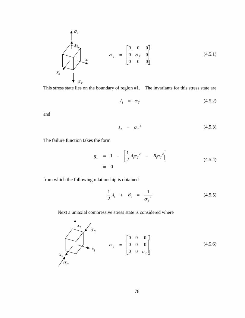
78
000
00
000
Tij (4.5.1)
This stress state lies on the boundary of region #1. The invariants for this stress state are
TI 1 (4.5.2)
and
22 TI (4.5.3)
The failure function takes the form
0
2
11 2
12
11
TT BAg
(4.5.4)
from which the following relationship is obtained
211
1
2
1
T
BA
(4.5.5)
Next a uniaxial compressive stress state is considered where
C00
000
000
ij
(4.5.6)
1x
2x
3x
T
T
1x
2x
3x
C
C

79
The principal stress direction for this stress state is
)1,0,0(ia (4.5.7)
thus
100
000
000
ji aa (4.5.8)
The invariants are as follows
CI 1 (4.5.9)
22 CI (4.5.10)
CI 4 (4.5.11)
and
25 CI (4.5.12)
Thus
0
12
1 22
22
222
CCC DBAg (4.5.13)
which leads to
2222
1
2
1
C
DBA
(4.5.14)
Next consider an equal biaxial compressive stress state where
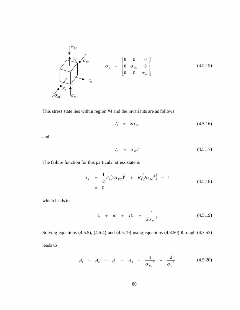
80
BC
BC
00
00
000
ij
(4.5.15)
This stress state lies within region #4 and the invariants are as follows
BCI 21 (4.5.16)
and
22 BCI (4.5.17)
The failure function for this particular stress state is
0
1222
1 24
244
BCBC BAf (4.5.18)
which leads to
2211
2
1
BC
DBA
(4.5.19)
Solving equations (4.5.5), (4.5.4) and (4.5.19) using equations (4.3.50) through (4.3.53)
leads to
224321
21
CBC
AAAA
(4.5.20)
1x
2x
3x
BC
BC
BCBC

81
22221
1
2
11
CBCT
BB
(4.5.21)
2243
2
12
BCC
BB
(4.5.22)
and
2232
11
TC
DD
(4.5.23)
In order to visualize the isotropic failure criterion relative to failure data from
Burchell et al. (2007), values were computed for the strength parameters identified
immediately above, i.e., T = 15.93 MPa for tension, C = -52.93 MPa for compression
and BC = -61.40 MPa for the biaxial compression. The values for T and C and were
obtained directly from Burchell et al. (2007). The value for BC was determined by a
best fit approximation of the failure curve to the data in Figure 4.5.1. Various
projections of the isotropic failure criterion are presented in the next several figures along
with the data from Burchell et al. (2007). The first is a projection onto the 11 – 22
stress space which is depicted in Figure 4.5.1. As can be seen in this figure the isotropic
failure model captures the different behavior in tension and compression exhibited by the
data from Burchell et al. (2007) along the 22 axis. However, the isotropic failure
criterion does not capture material anisotropy which is clearly exhibited by the failure
data from Burchell et al. (2007) along the tensile segments of the 11 axis relative to the
22 axis.
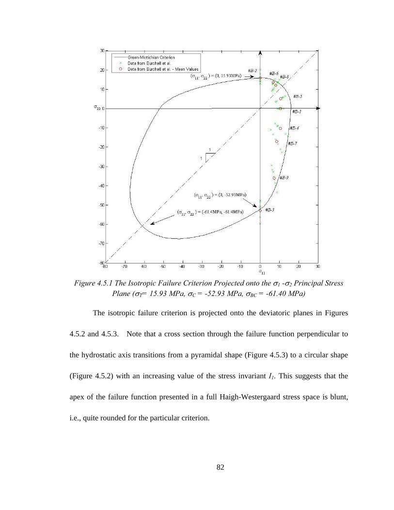
82
Figure 4.5.1 The Isotropic Failure Criterion Projected onto the 1 -2 Principal Stress
Plane (T= 15.93 MPa, C = -52.93 MPa, BC = -61.40 MPa)
The isotropic failure criterion is projected onto the deviatoric planes in Figures
4.5.2 and 4.5.3. Note that a cross section through the failure function perpendicular to
the hydrostatic axis transitions from a pyramidal shape (Figure 4.5.3) to a circular shape
(Figure 4.5.2) with an increasing value of the stress invariant I1. This suggests that the
apex of the failure function presented in a full Haigh-Westergaard stress space is blunt,
i.e., quite rounded for the particular criterion.
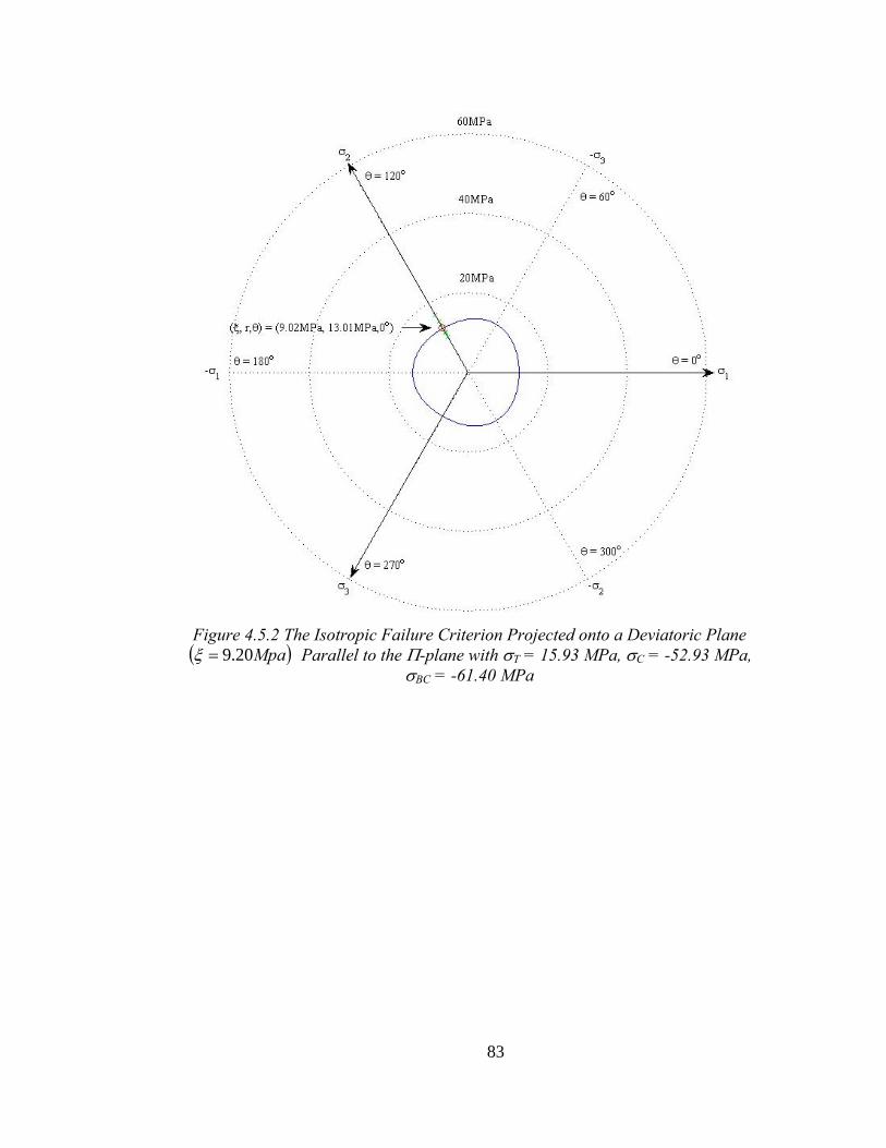
83
Figure 4.5.2 The Isotropic Failure Criterion Projected onto a Deviatoric Plane Mpa20.9 Parallel to the -plane with T = 15.93 MPa, C = -52.93 MPa,
BC = -61.40 MPa
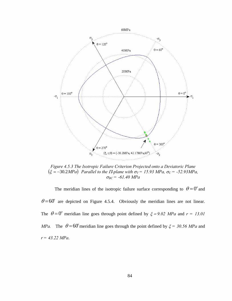
84
Figure 4.5.3 The Isotropic Failure Criterion Projected onto a Deviatoric Plane MPa2.30 Parallel to the -plane with T = 15.93 MPa, C = -52.93MPa,
BC = -61.40 MPa
The meridian lines of the isotropic failure surface corresponding to o0 and
o60 are depicted on Figure 4.5.4. Obviously the meridian lines are not linear.
The o0 meridian line goes through point defined by 9.02 MPa and r = 13.01
MPa. The o60 meridian line goes through the point defined by = 30.56 MPa and
r = 43.22 MPa.
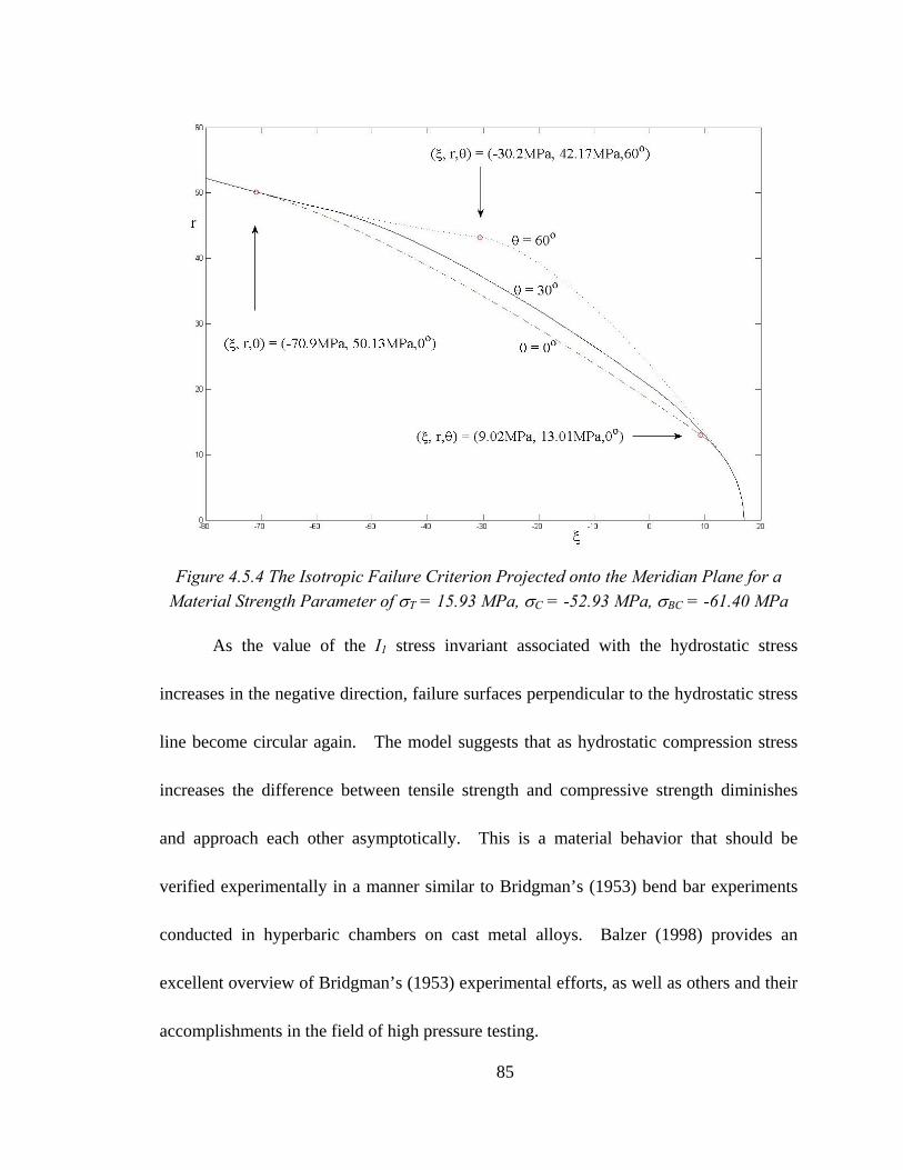
85
Figure 4.5.4 The Isotropic Failure Criterion Projected onto the Meridian Plane for a
Material Strength Parameter of T = 15.93 MPa, C = -52.93 MPa, BC = -61.40 MPa
As the value of the I1 stress invariant associated with the hydrostatic stress
increases in the negative direction, failure surfaces perpendicular to the hydrostatic stress
line become circular again. The model suggests that as hydrostatic compression stress
increases the difference between tensile strength and compressive strength diminishes
and approach each other asymptotically. This is a material behavior that should be
verified experimentally in a manner similar to Bridgman’s (1953) bend bar experiments
conducted in hyperbaric chambers on cast metal alloys. Balzer (1998) provides an
excellent overview of Bridgman’s (1953) experimental efforts, as well as others and their
accomplishments in the field of high pressure testing.

86
However, as indicated in Figure 4.5.1, the isotropic formulation of the failure
criterion does not capture the anisotropic behavior of the data from Burchell et al. (2007).
The isotropic formulation is extended to transverse isotropy in the next chapter.
Orthotropic behavior and other types of anisotropic behavior can be captured through
similar use of tensorial invariants.
87
CHAPTER V
ANISOTROPIC FAILURE CRITERION
As discussed in earlier sections the multiaxial failure data from Burchell et al.
(2007) strongly suggests that the graphite tested was anisotropic. Thus there is a need to
extend the isotropic failure model discussed in the previous section so that anisotropic
failure behavior is captured. This can be done again by utilizing stress based invariants
where the material anisotropy is captured through the use of a direction vector associated
with primary material directions. The concept is identical to the extension of the
isotropic inelastic constitutive model. The extension of a phenomenological failure
criterion will be made for a transversely isotropic material. Other material symmetries,
e.g., an orthotropic material symmetry, can be included as well. Duffy and
Manderscheid (1990b) as well as others have suggested an appropriate integrity basis for
the orthotropic material symmetry. Transversely isotropic materials have the same
properties in one plane and different properties in a direction normal to this plane.
Orthotropic materials have different properties in three mutually perpendicular directions.
88
5.1 Integrity Base for Anisotropy
The preferred material direction is designated through a second direction vector,
di. The dependence of the failure function is extended such that
0,, jijiij aaddg (5.1.1)
The definition of the unit vector ai is the same as in earlier sections. Rivlin and Smith
(1969) as well as Spencer (1971) show that for a scalar valued function with dependence
stipulated by equation (5.1.1) the integrity basis is
kkI 1 (5.1.2)
jiijI 2 (5.1.3)
kijkijI 3 (5.1.4)
ijji aaI 4 (5.1.5)
kijkji aaI 5 (5.1.6)
jiji ddI 6 (5.1.7)
kijkji ddI 7 (5.1.8)
kjkjji ddaaI 8 (5.1.9)
and
mikmkjji ddaaI 9 (5.1.10)
The invariant I3 is omitted again since this invariant is cubic in stress. As before those
invariants linear in stress enter the functional dependence as squared terms or as products
89
with another invariant linear in stress. Therefore the anisotropic failure function has the
following dependence
981761
54122
1
98765421
2
11
,,,,,,,,,
HIIGIFIIEI
DIICIBIAI
IIIIIIIIgaaddg jijiij
(5.1.11)
The form of the failure function was constructed as a polynomial in the invariants listed
above. The constants in this formulation (A, B, C, D, E, F, G, and H) are characterized
by adopting simple strength tests. The proposed failure function was incorporated into a
reliability model through the use of Monte Carlo simulation and importance sampling
techniques. This feature is discussed in a subsequent section.
5.2 Functional Forms and Associated Gradients by Stress Region
Similar to the approach adopted for anisotropic constitutive models, the
underlying concept is that the response of the material depends on the stress state, a
preferred material direction and whether the principal stresses are tensile or compressive.
The principal stress space is divided again into four regions. The regions and associated
failure functions are listed below. In the first region all of the principal stresses are
tensile, i.e.,
Region #1: 0321
7161121
2111 2
11 IFIIEIBIAg (5.2.1)
90
In Region #1 a direction vector associated with the principal stresses is unnecessary since
all principal stresses are tensile. The corresponding normal to the failure surface is
ijijijijij
I
I
gI
I
gI
I
gI
I
gg
7
7
16
6
12
2
11
1
11 (5.2.2)
where
61111
1 IEIAI
g
(5.2.3)
12
1 BI
g
(5.2.4)
116
1 IEI
g
(5.2.5)
17
1 FI
g
(5.2.6)
ijij
I
1 (5.2.7)
ijij
I
22
(5.2.8)
jiij
ddI
6 (5.2.9)
and
jkkikijkij
ddddI
7 (5.2.10)

91
Substitution of equations (5.2.3) through (5.2.10) into (5.2.2) leads to the following
tensor expression
kikjjkik
jiijijij
ddddF
ddIEBIEIAg
1
11161111 2
(5.2.11)
or
kikjjkik
ijjiijijij
ddddF
IddIEBIAg
1
6111111 2
(5.2.12)
Region #2: 321 0
9281272612
52412222
122 2
11
IHIIGIFIIE
IDIICIBIAg
(5.2.13)
In Region #2 the direction vector ai is associated with the compressive principal stress σ3.
Thus for this region
1,0,0ia (5.2.14)
.The corresponding normal to the failure surface is
ijijijij
ijijijijij
I
I
gI
I
gI
I
gI
I
g
I
I
gI
I
gI
I
gI
I
gg
9
9
28
8
27
7
26
6
2
5
5
24
4
22
2
21
1
22
(5.2.15)
where
826242121
2 IGIEICIAI
g
(5.2.16)
92
22
2 BI
g
(5.2.17)
124
2 ICI
g
(5.2.18)
25
2 DI
g
(5.2.19)
126
2 IEI
g
(5.2.20)
27
2 FI
g
(5.2.21)
128
2 IGI
g
(5.2.22)
2
9
2 HI
g
(5.2.23)
jiij
aaI
4 (5.2.24)
kikjjkikij
aaaaI
5 (5.2.25)
jkkiij
ddaaI
8 (5.2.26)
and
jkkllikijllkij
ddaaddaaI
9 (5.2.27)
93
Substitution of equations (5.2.7) through (5.2.10) and (5.2.16) through (5.2.27) into
(5.2.15) leads to the following tensor expression
jkkllikijllkjkki
jkkikijkji
kikjjkikji
ijijij
ddaaddaaHddaaIG
ddddFddIE
aaaaDaaIC
BIGIEICIAg
212
212
212
2826242122 2
(5.2.28)
then
jkkllikijllk
ijjkkijkkikijk
ijjikikjjkik
ijjiijijij
ddaaddaaH
IddaaIGddddF
IddIEaaaaD
IaaICBIAg
2
8122
6122
4122122 2
(5.2.29)
Region #3: 321 0
The failure function for this region of the stress space is
938133613
753413232
133 2
11
IHIIGFIIE
IIDIICIBIAg
(5.2.30)
In Region #3 the direction vector ai is associated with the tensile principal stress direction
σ1. For this region
0,0,1ia (5.2.31)
.The corresponding normal to the failure surface is
ijijijij
ijijijijij
I
I
gI
I
gI
I
gI
I
g
I
I
gI
I
gI
I
gI
I
gg
9
9
38
8
37
7
36
6
3
5
5
34
4
32
2
31
1
33
(5.2.32)

94
where
836343131
3 IGIEICIAI
g
(5.2.33)
32
3 BI
g
(5.2.34)
134
3 ICI
g
(5.2.35)
35
3 DI
g
(5.2.36)
136
3 IEI
g
(5.2.37)
37
3 FI
g
(5.2.38)
138
3 IGI
g
(5.2.39)
and
39
3 HI
g
(5.2.40)
Substitution of equations (5.2.7) through (5.2.10), (5.2.24) through (5.2.27) and (5.2.33)
through (5.2.40) into (5.2.32) leads to the following tensor expression
jkkllikijllkjkki
jkkikijkji
kikjjkikji
ijijij
ddaaddaaHddaaIG
ddddFddIE
aaaaDaaIC
BIGIEICIAg
313
313
313
3836343133 2
(5.2.41)
or

95
jkkllikijllk
ijjkkijkkikijk
ijjikikjjkik
ijjiijijij
ddaaddaaH
IddaaIGddddF
IddIEaaaaD
IaaICBIAg
3
8133
6133
4133133 2
(5.2.42)
Region #4: 3210
The failure function for this region of the stress space is
7461424
2144 2
11 IFIIEIBIAg (5.2.43)
and since all principal stresses are compressive a direction vector associated with the
principal stress direction is unnecessary. The corresponding normal to the failure
surface is
ijijijijij
I
I
gI
I
gI
I
gI
I
gg
7
7
46
6
42
2
41
1
44 (5.2.44)
where
64141
4 IEIAI
g
(5.2.45)
42
4 BI
g
(5.2.46)
146
4 IEI
g
(5.2.47)
47
4 FI
g
(5.2.48)
and

96
47
4 FI
g
(5.2.49)
Substitution of equations (5.2.7) through (5.2.10) and (5.2.45) through (5.2.49) into
(5.2.44) leads to the following tensor expression
kikjjkik
jiijijij
ddddF
ddIEBIEIAg
1
11161114 2
(5.2.50)
or
kikjjkik
ijjiijijij
ddddF
IddIEBIAg
1
6111114 2
(5.2.51)
5.3 Relationships Between Functional Constants
With the failure functions and the normals to those functions defined in general
terms for each region, attention is now turned to establishing functional relationships
between the constants. Consider the following stress state at failure under a tensile load
in the preferred material direction with material direction di = (0, 1, 0), i.e.,
000
00
000
YTij (5.3.1)
1x
2x
3x
YT
YT
id
97
The first stress subscript Y denotes a strength parameter associated with the strong
direction, and second subscript T denotes this quantity is a tensile strength
parameterThe principal stresses for this stress state are
0,0,,, 321 YT (5.3.2)
and this stress state lies along the boundary shared by region #1 and region #2, as well as
the shared boundary along region #2 and region #3. At both boundaries we impose the
requirements that the gradients match, i.e.,
ijij
gg
21 (5.3.3)
ijij
gg
32 (5.3.4)
providing a smooth transition from one principal stress region to another. For this stress
state the first, second, sixth and seventh invariants of stress are
YTI 1 (5.3.5)
22 YTI (5.3.6)
YTI 6 (5.3.7)
and
27 YTI (5.3.8)
These stress invariants are common for stress region #1, #2 and #3. With these
invariants

98
11
111
000
020
000
00
020
00
000
020
000
00
00
00
FE
BAg
YT
YT
YT
YT
YT
YT
YT
YT
ij
(5.3.9)
For the stress state in region #2 given above the unit principal stress vector is
)1,0,0(2 ia (5.3.10)
The left superscript “2” denotes a vector associated with principal stress region #2. Thus
100
000
00022
ji aa (5.3.11)
The stress invariants associated with this vector and the stress state given above are
042 I (5.3.12)
052 I (5.3.13)
082 I (5.3.14)
and
092 I (5.3.15)
With these stress invariants and stress state the gradient along the boundary for stress
region #2 is
99
22
2222
000
020
000
00
020
00
00
000
000
000
020
000
00
00
00
FE
CBAg
YT
YT
YT
YT
YT
YT
YT
YT
YT
ij
(5.3.16)
Utilizing equations (5.3.9) and (5.3.16) in equation (5.3.3) then at the boundary between
stress region #1 and stress region #2
222
22
11
11
000
020
000
00
020
00
00
000
000
000
020
000
00
00
00
000
020
000
00
020
00
000
020
000
00
00
00
FEC
BA
FE
BA
YT
YT
YT
YT
YT
YT
YT
YT
YT
YT
YT
YT
YT
YT
YT
YT
YT
(5.3.17)
The following three expressions can be extracted from equation (5.3.17), i.e.,
2211 EAEA (5.3.18)
22221111 222222 FEBAFEBA (5.3.19)
and
22211 ECAEA (5.3.20)
For the stress state in region #3 given above the unit principal stress vector is
)0,1,0(3 ia (5.3.21)

100
Thus
000
010
00033
ji aa (5.3.22)
The stress invariants associated with this unit vector and stress state are
YTI 43 (5.3.23)
25
3YTI (5.3.24)
YTI 83 (5.3.25)
and
29
3YTI (5.3.26)
With these stress invariants and stress state the gradient along the boundary for stress
region #3 is
3
33
33
333
000
020
000
00
020
00
000
020
000
00
020
00
00
020
00
000
020
000
00
00
00
H
GF
EC
BAg
YT
YT
YT
YT
YT
YT
YT
YT
YT
YT
YT
YT
YT
YT
YT
ij
(5.3.27)
Utilizing equations (5.3.16) and (5.3.27) in equation (5.3.4) then at the boundary between
stress region #2 and stress region #3
101
333
333
33
222
22
000
020
000
00
020
00
000
020
000
00
020
00
000
020
000
00
020
00
000
020
000
00
00
00
000
020
000
00
020
00
00
000
000
000
020
000
00
00
00
HGF
EDC
BA
FEC
BA
YT
YT
YT
YT
YT
YT
YT
YT
YT
YT
YT
YT
YT
YT
YT
YT
YT
YT
YT
YT
YT
YT
YT
YT
YT
(5.3.28)
The following three expressions can be extracted from equation (5.3.28), i.e.,
333322 GECAEA (5.3.29)
3333
3333
2222
2222
222
222
HGFE
DCBA
FEBA
(5.3.30)
and
3333222 GECAECA (5.3.31)
Next consider the following stress state at failure under a compression load with
the same material direction di = (0, 1, 0) as above, i.e.,
000
00
000
YCij (5.3.32) 1x
2x
3x
idYC
YC
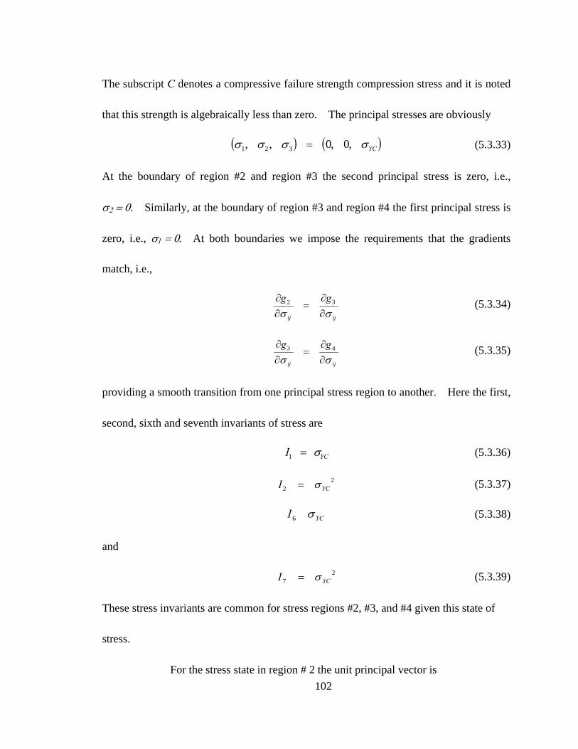
102
The subscript C denotes a compressive failure strength compression stress and it is noted
that this strength is algebraically less than zero. The principal stresses are obviously
YC ,0,0,, 321 (5.3.33)
At the boundary of region #2 and region #3 the second principal stress is zero, i.e.,
. Similarly, at the boundary of region #3 and region #4 the first principal stress is
zero, i.e., At both boundaries we impose the requirements that the gradients
match, i.e.,
ijij
gg
32 (5.3.34)
ijij
gg
43 (5.3.35)
providing a smooth transition from one principal stress region to another. Here the first,
second, sixth and seventh invariants of stress are
YCI 1 (5.3.36)
22 YCI (5.3.37)
YCI 6 (5.3.38)
and
27 YCI (5.3.39)
These stress invariants are common for stress regions #2, #3, and #4 given this state of
stress.
For the stress state in region # 2 the unit principal vector is

103
)0,1,0(2 ia (5.3.40)
thus
000
010
00022
ji aa (5.3.41)
The stress invariants associated with this unit vector and stress state are
YCI 42 (5.3.42)
25
2YCI (5.3.43)
YCI 82 (5.3.44)
and
29
2YCI (5.3.45)
With these stress invariants and stress state, the gradient along the boundary for stress
region #2 is
22
22
22
222
000
020
000
00
020
00
000
020
000
00
020
00
000
020
000
00
020
00
000
020
000
00
00
00
HG
FE
DC
BAg
YC
YC
YC
YC
YC
YC
YC
YC
YC
YC
YC
YC
YC
YC
YC
YC
ij
(5.3.46)
As noted earlier the unit vector associated with region #3 is
104
)0,0,1(3 ia (5.3.47)
thus
000
000
00133
ji aa (5.3.48)
The stress invariants associated with this unit vector and stress state are
043 I (5.3.49)
053 I (5.3.50)
083 I (5.3.51)
and
093 I (5.3.52)
With these stress invariants and stress state, the gradient along the boundary for stress
region #3 is
33
3333
000
020
000
00
020
00
000
000
00
000
020
000
00
00
00
FE
CBAg
YC
YC
YC
YC
YC
YC
YC
YC
YC
ij
(5.3.53)
Utilizing equations (5.3.46) and (5.3.53) in equation (5.3.34) then at the boundary
between stress region #2 and stress region #3

105
33
333
22
222
222
000
020
000
00
020
00
000
000
00
000
020
000
00
00
00
000
020
000
00
020
00
000
020
000
00
020
00
000
020
000
00
020
00
000
020
000
00
00
00
FE
CBA
HG
FED
CBA
YC
YC
YC
YC
YC
YC
YC
YC
YC
YC
YC
YC
YC
YC
YC
YC
YC
YC
YC
YC
YC
YC
YC
YC
YC
(5.3.54)
The following three expressions can be extracted from equation (5.3.54), i.e.,
3332222 ECAGECA (5.3.55)
3333
2222
2222
222
2222
222
FEBA
HGFE
DCBA
(5.3.56)
and
332222 EAGECA (5.3.57)
With the invariants established in equations (5.3.36) through (5.3.39), the
following gradient for region #3 takes the following form

106
44
444
000
020
000
00
020
00
000
020
000
00
00
00
FE
BAg
YC
YC
YC
YC
YC
YC
YC
YC
ij
(5.3.58)
Utilizing equations (5.3.53) and (5.3.58) in equation (5.3.35) then at the boundary
between principal stress region #3 and principal stress region #4
44
44
333
33
000
020
000
00
020
00
000
020
000
00
00
00
000
020
000
00
020
00
000
000
00
000
020
000
00
00
00
FE
BA
FEC
BA
YC
YC
YC
YC
YC
YC
YC
YC
YC
YC
YC
YCYC
YC
YC
YC
YC
(5.3.59)
The following three expressions can be extracted from equation (5.3.59), i.e.,
44333 EAECA (5.3.60)
44443333 222222 FEBAFEBA (5.3.61)
and
4433 EAEA (5.3.62)
Next consider the following stress state at failure under a tensile load with the
same preferred material direction di = (0, 1, 0), i.e.,
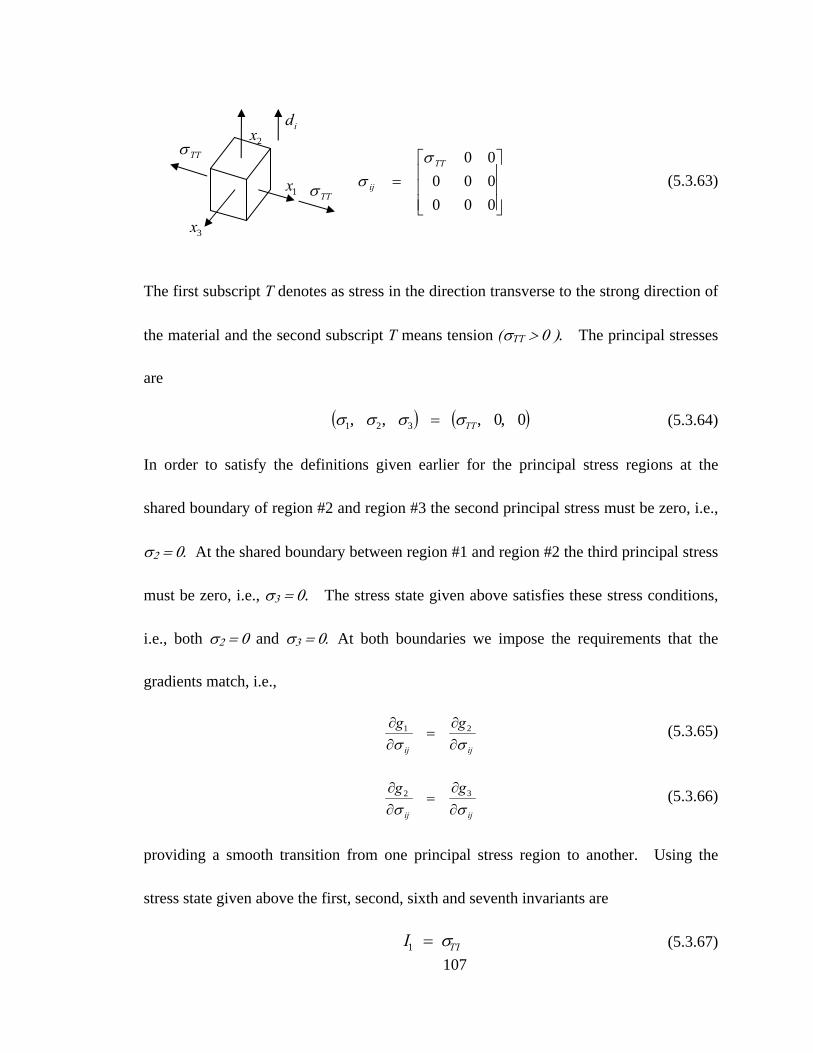
107
000
000
00TT
ij
(5.3.63)
The first subscript T denotes as stress in the direction transverse to the strong direction of
the material and the second subscript T means tension (TT. The principal stresses
are
0,0,,, 321 TT (5.3.64)
In order to satisfy the definitions given earlier for the principal stress regions at the
shared boundary of region #2 and region #3 the second principal stress must be zero, i.e.,
At the shared boundary between region #1 and region #2 the third principal stress
must be zero, i.e., . The stress state given above satisfies these stress conditions,
i.e., both and At both boundaries we impose the requirements that the
gradients match, i.e.,
ijij
gg
21 (5.3.65)
ijij
gg
32 (5.3.66)
providing a smooth transition from one principal stress region to another. Using the
stress state given above the first, second, sixth and seventh invariants are
TTI 1 (5.3.67)
1x
2x
3x
id
TT
TT

108
22 TTI (5.3.68)
06 I (5.3.69)
and
07 I (5.3.70)
These four invariants are common to stress regions #1, #2 and #3 for the stress state
given above. With these stress invariants the following gradient can be formulated for
this stress state
11
11
000
00
000
000
000
002
00
00
00
EB
Ag
TT
TT
TT
TT
TT
ij
(5.3.71)
For the stress state in region # 2 the unit principal vector is
)1,0,0(2 ia (5.3.72)
Thus
100
000
00022
ji aa (5.3.73)
The invariants associated with this principal stress vector and stress state are
042 I (5.3.74)
052 I (5.3.75)
082 I (5.3.76)
109
and
092 I (5.3.77)
With these invariants and stress state the gradient along the boundary for stress region #2
is
22
222
000
00
000
00
000
000
000
000
002
00
00
00
EC
BAg
TT
TT
TT
TT
TT
TT
ij
(5.3.78)
Utilizing equations (5.71) and (5.3.78) in equation (5.3.65) then at the boundary between
principal stress region #1 and principal stress region #2
2
222
111
000
00
000
00
000
000
000
000
002
00
00
00
000
00
000
000
000
002
00
00
00
E
CBA
EBA
TT
TT
TT
TT
TT
TT
TT
TT
TT
TT
TT
(5.3.79)
The following three relationships between functional constants can be extracted from
equation (5.3.79)
22211 222 CBABA (5.3.80)
2211 EAEA (5.3.81)
and

110
221 CAA (5.3.82)
For the stress state stipulated above the unit principal vector in region # 3 is
)0,0,1(3 ia (5.3.83)
thus
000
000
00133
ji aa (5.3.84)
And the stress invariants for this principal stress vector and stress state are
TTI 43 (5.3.85)
25
3TTI (5.3.86)
083 I (5.3.87)
and
093 I (5.3.88)
With these invariants and stress state the gradient along the boundary for stress region #3
is
333
333
000
00
000
000
000
002
00
00
002
000
000
002
00
00
00
EDC
BAg
TT
TT
TT
TT
TT
TT
TT
TT
TT
ij
(5.3.89)
Utilizing equations (5.78) and (5.3.89) in equation (5.3.66) then at the boundary between
principal stress region #2 and principal stress region #3

111
333
33
22
22
000
00
000
000
000
002
00
00
002
000
000
002
00
00
00
000
00
000
00
000
000
000
000
002
00
00
00
EDC
BA
EC
BA
TT
TT
TT
TT
TT
TT
TT
TT
TT
TT
TT
TT
TT
TT
TT
(5.3.90)
The following three expressions can be extracted from equation (5.3.90)
333322 2222 DCBABA (5.3.91)
33322 ECAEA (5.3.92)
and
3322 CACA (5.3.93)
Next consider the following stress state at failure under a compressive load with
the preferred material direction di = (0, 1, 0), i.e.,
000
000
00TC
ij
(5.3.94)
1x
2x
3x
id
TC
TC
112
The first subscript T denotes a stress in the direction transverse to the strong direction of
the material, and the second subscript C denotes compression (TC. The principal
stresses are
TC ,0,0,, 321 (5.3.95)
In order to satisfy the definitions given earlier for the principal stress regions at the
shared boundary of region #3 and region #4 the first principal stress must be zero, i.e.,
At the shared boundary between region #2 and region #3 the second principal
stress must be zero, i.e., . The stress state given above satisfies these stress
conditions, i.e., both and At both boundaries we impose the requirements
that the gradients match, i.e.,
ijij
gg
32 (5.3.96)
ijij
gg
43 (5.3.97)
providing a smooth transition from one principal stress region to another. Using the
stress state given above the first, second, sixth and seventh invariants are
TCI 1 (5.3.98)
22 TCI (5.3.99)
06 I (5.3.100)
and
07 I (5.3.101)

113
These four invariants are common to stress regions #2, #3 and #4 for the stress state
given above. With these stress invariants the following gradient can be formulated for
this stress state
44
44
000
00
000
000
000
002
00
00
00
EB
Ag
TC
TC
TC
TC
TC
ij
(5.3.102)
For the stress state in region # 2 the unit principal vector is
)0,0,1(2 ia (5.3.103)
Thus
000
000
00122
ji aa (5.3.104)
The stress invariants for this principal stress vector are
TCI 42 (5.3.105)
25
2TCI (5.3.106)
082 I (5.3.107)
and
092 I (5.3.108)
With these stress invariants the following gradient can be formulated for this stress state

114
222
222
000
00
000
000
000
002
00
00
002
000
000
002
00
00
00
EDC
BAg
TC
TC
TC
TC
TC
TC
TC
TC
TC
ij
(5.3.109)
For the stress state in region #3 the unit principal vector is
)0,1,0(3 ia (5.3.110)
Thus
000
010
00033
ji aa (5.3.111)
And the stress invariants for this principal stress vector are
043 I (5.3.112)
053 I (5.3.113)
083 I (5.3.114)
and
093 I (5.3.115)
With these stress invariants the following gradient can be formulated for this stress state
33
333
000
00
000
000
00
000
000
000
002
00
00
00
EC
BAg
TCTC
TC
TC
TC
TC
ij
(5.3.116)
115
Utilizing equations (5.116) and (5.3.109) in equation (5.3.96) then at the boundary
between principal stress region #2 and principal stress region #3
33
33
222
22
000
00
000
000
00
000
000
000
002
00
00
00
000
00
000
000
000
002
00
00
002
000
000
002
00
00
00
EC
BA
EDC
BA
TCTC
TC
TC
TC
TC
TC
TC
TC
TC
TC
TC
TC
TC
TC
(5.3.117)
The following three expressions can be extracted from equation (5.3.117), i.e.,
332222 2222 BADCBA (5.3.118)
333222 ECAECA (5.3.119)
and
322 ACA (5.3.120)
Utilizing equations (5.102) and (5.3.116) in equation (5.3.97) then at the boundary
between principal stress region #3 and principal stress region #4
116
44
4
33
33
000
00
000
000
000
002
00
00
00
000
00
000
000
00
000
000
000
002
00
00
00
EB
A
EC
BA
TC
TC
TC
TC
TC
TCTC
TC
TC
TC
TC
(5.3.121)
The following three expressions can be extracted from equation (5.3.121)
4433 22 BABA (5.3.122)
44333 EAECA (5.3.123)
and
43 AA (5.3.124)
Equations (5.3.18) through (5.3.20), (5.3.29) through (5.3.31), (5.3.55) through (5.3.57),
(5.3.60) through (5.3.62), (5.3.80) through (5.3.82), (5.3.91) through (5.3.93), (5.3.118)
through (5.3.120), as well as (5.3.122) through (5.3.124) represent twenty four equations
in terms of twenty four unknowns, i.e., A1, A2, A3, A4, B1, B2, B3, B4, C2, C3, D2, D3, E1, E2,
E3, E4, F1, F2, F3, F4, G2, G3, H2 and H3.
Although in the current formulation there appears to be twenty-four constants, not
all of the constants are independent. From equations (5.3.18) and (5.3.20) it is apparent
that
117
02 C (5.3.125)
Substitution of equation (5.3.125) into equations (5.3.82) yields
21 AA (5.3.126)
Substitution of equation (5.3.125) into equation (5.3.120) yields
32 AA (5.3.127)
With equation (5.3.124) then
4321 AAAA (5.3.128)
Thus none of the “A” constants are independent.
Substitution of equation (5.3.125) and (5.3.127) into equation (5.3.93) leads to
03 C (5.3.129)
Using equation (5.3.129) along with equation (5.3.128) in equation (5.3.60) results in
43 EE (5.3.130)
Substitution of equation (5.3.126) into equation (5.3.18) yields
21 EE (5.3.131)
Substituting equations (5.3.125), (5.3.125) and (5.3.125) into equation (5.3.119) results in
32 EE (5.3.132)
With equations (5.3.130), (5.3.131) and (5.3.132) then
4321 EEEE (5.3.133)
Therefore none of the “E” constants are independent.
118
Substitution of equations (5.3.125), (5.3.127) and (5.3.133) into equations (5.3.57)
leads to
02 G (5.3.134)
Similarly substituting equations (5.3.127), (5.3.129) and (5.3.133) into equation (5.3.29)
leads to
03 G (5.3.135)
and the “G” constants are both zero.
With equations (5.3.125) and (5.3.126) then from equation (5.3.80) takes the form
21 BB (5.3.136)
Utilizing equation (5.3.128) in equation (5.3.122) then
43 BB (5.3.137)
With equations (5.3.127) and (5.3.129) then equation (5.3.91) takes the form
332 DBB (5.3.138)
Similarly, with equations (5.3.125) and (5.3.127) then equation (5.3.118) takes the form
322 BDB (5.3.139)
Subtracting equation (5.3.138) from equation (5.3.139) leads to
32 DD (5.3.140)
and the “D” constants are not independent of one another.
With equations (5.3.126), (5.3.136) and (5.3.131) then equation (5.3.19) takes the
form
119
21 FF (5.3.141)
With equations (5.3.128), (5.3.137) and (5.3.130) then from equation (5.3.61)
43 FF (5.3.142)
In a like manner, with equations (5.3.127), (5.3.132), (5.3.129) and (5.3.135) then
equation (5.3.30) takes the form
332 HFF (5.3.143)
With equations (5.3.127), (5.3.132), (5.3.125) and (5.3.134) then equation (5.3.56) takes
the form
322 FHF (5.3.144)
Subtracting equation (5.3.143) from equation (5.3.144) leads to
32 HH (5.3.145)
From equations (5.3.125) and (5.3.129) the identity
032 CC (5.3.148)
can be established. From equations (5.3.134) and (5.3.155) it is easily shown that
032 GG (5.3.152)
In addition, the following relationships between the remaining coefficients are
established from equations (5.3.125) through (5.3.145)
A 4321 AAAA (5.3.146)
B 343321 DBDBBB (5.3.147)
D 32 DD (5.3.148)

120
E 4321 EEEE (5.3.149)
F 343321 HFHFFF (5.3.150)
and
H 32 HH (5.3.151)
These relationships represent requirements that insure the four functional forms for the
failure function are smooth and continuous along the boundaries of the four stress
regions. Moreover, the last group of constants identified as A, B, D, E, F and H
represent the independent constants for the failure function. Since there are six
independent constants, then one is required to conduct six mechanical tests to
characterize the model. These tests are outlined in the next section.
5.4 Functional Constants in Terms of Strength Parameters
Next specific load paths are utilized in order to define the constants defined above
in terms of strength values obtained in mechanical failure tests. Consider the following
stress state at failure under a uniaxial tensile load in the preferred material direction di =
(0, 1, 0)
000
00
000
YTij (5.4.1)
1x
2x
3x
YT
YT
id

121
The principal stresses for this state of stress are
0,0,,, 321 YT (5.4.2)
Note that one principal stress is tensile and the others are zero. This state of stress lies
along the border of region #1, region #2 and region #3. For region #1 the first, second,
sixth and seventh invariants are
YTI 1 (5.4.3)
22 YTI (5.4.4)
YTI 6 (5.4.5)
and
27 YTI (5.4.6)
With the failure function defined as
0
2
11 7161121
2111
IFIIEIBIAg (5.4.7)
in region #1 of the principal stress space, then substitution of equations (5.4.3) through
(5.4.6) into the (5.4.7) yields
2
112
12
12
110 YTYTYTYTYT FEBA (5.4.8)
or
21111
1
2
1
YT
FEBA
(5.4.9)
The unit principal stress vector associated with this state of stress in the region # 2
is

122
)1,0,0(2 ia (5.4.10)
thus
100
000
00022
ji aa (5.4.11)
The stress invariants associated with this principal stress vector and state of stress are
042 I (5.4.12)
052 I (5.4.13)
082 I (5.4.14)
and
092 I (5.4.15)
The failure function for stress region #2 has the form
0
2
11
9281272612
52412222
122
IHIIGIFIIE
IDIICIBIAg
(5.4.16)
With equations (5.4.3) through (5.4.6) as well as equations (5.4.12) through (5.4.15) then
2
222
22
22
110 YTYTYTYTYT FEBA (5.4.17)
or
22222
1
2
1
YT
FEBA
(5.4.18)
123
The unit principal stress vector associated with this state of stress in the region # 3
is
)0,1,0(3 ia (5.4.19)
thus
000
010
00033
ji aa (5.4.20)
The stress invariants associated with this principal stress vector and state of stress are
YTI 43 (5.4.21)
25
3YTI (5.4.22)
YTI 83 (5.4.23)
and
29
3YTI (5.4.24)
The failure function for stress region #3 has the form
0
2
11
938133613
753413232
133
IHIIGFIIE
IIDIICIBIAg
(5.4.25)
With equations (5.4.3) through (5.4.6) as well as equations (5.4.21) through (5.4.24) then
23
233
23
23
232
110
YTYTYTYT
YTYTYT
HFE
DBA
(5.4.26)
and
124
2333333
1
2
1
YT
HFEDBA
(5.4.27)
Next consider the following stress state at failure due to a compressive stress
aligned with the material direction di = (0, 1, 0), i.e.,
000
00
000
YCij (5.4.28)
The principal stresses are
YC ,0,0,, 321 (5.4.29)
Note that one principal stress is compressive and the others are zero. This state of stress
lies along the border of region #2, region #3 and region #4. For region #4 the first,
second, sixth and seventh invariants for this stress state are
YCI 1 (5.4.30)
22 YCI (5.4.31)
YCI 6 (5.4.32)
and
27 YCI (5.4.33)
With the failure function defined as
1x
2x
3x
idYC
YC
125
0
2
11 7461424
2144
IFIIEIBIAg
(5.4.34)
in region #4 of the principal stress space, then substitution of equations (5.4.30) through
(5.4.33) into the (5.4.34) yields
2
442
42
42
110 YCYCYCYCYC FEBA (5.4.35)
or
24444
1
2
1
YC
FEBA
(5.4.36)
The unit principal stress vector associated with this state of stress in region #2 is
)0,1,0(2 ia (5.4.37)
thus
000
010
00022
ji aa (5.4.38)
The stress invariants associated with this principal stress vector and state of stress are
YCI 42 (5.4.39)
25
2YCI (5.4.40)
YCI 82 (5.4.41)
and
29
2YCI (5.4.42)
Again, the failure function for stress region #2 has the form
126
0
2
11
9281272612
52412222
122
IHIIGIFIIE
IDIICIBIAg
(5.4.43)
With equations (5.4.30) through (5.4.33) as well as equations (5.4.39) through (5.4.42)
then
22
222
22
22
222
110
YCYCYCYC
YCYCYC
HFE
DBA
(5.4.44)
or
2222222
1
2
1
YC
HFEDBA
(5.4.45)
The unit principal stress vector associated with this state of stress in region #3 is
)0,0,1(3 ia (5.4.46)
thus
000
000
00133
ji aa (5.4.47)
The stress invariants associated with this principal stress vector and state of stress are
043 I (5.4.48)
053 I (5.4.49)
083 I (5.4.50)
and
093 I (5.4.51)

127
Again, the failure function for stress region #3 has the form
0
2
11
938133613
753413232
133
IHIIGFIIE
IIDIICIBIAg
(5.4.52)
With equations (5.4.30) through (5.4.33) as well as equations (5.4.48) through (5.4.51)
then
2
332
32
32
110 YCYCYCYCYC FEBA (5.4.53)
or
23333
1
2
1
YC
FEBA
(5.4.54)
Next consider the following stress state at failure due to a tensile stress
perpendicular to the material direction di = (0, 1, 0), i.e.,
000
000
00TT
ij
(5.4.55)
The principal stresses are
0,0,,, 321 TT (5.4.56)
Note that principal stress aligned transverse to the preferred direction of the material is
tensile and the others are zero. This state of stress lies along the border of region #1,
1x
2x
3x
id
TT
TT

128
region #2 and region #3. For region #1 the first, second, sixth and seventh invariants are
obtained
TTI 1 (5.4.57)
22 TTI (5.4.58)
06 I (5.4.59)
and
07 I (5.4.60)
Again, with the failure function defined as
0
2
11 7161121
2111
IFIIEIBIAg (5.4.61)
in region #1 of the principal stress space, then substitution of equations (5.4.57) through
(5.4.60) into the (5.4.61) leads to
2
12
12
110 TTTT BA (5.4.62)
or
211
1
2
1
TT
BA
(5.4.63)
The unit principal stress vector associated with this state of stress in region #2 is
)1,0,0(2 ia (5.4.64)
thus

129
100
000
00022
ji aa (5.4.65)
The stress invariants associated with this principal stress vector and state of stress are
042 I (5.4.66)
052 I (5.4.67)
082 I (5.4.68)
and
092 I (5.4.69)
Again, the failure function for stress region #2 has the form
0
2
11
9281272612
52412222
122
IHIIGIFIIE
IDIICIBIAg
(5.4.70)
With equations (5.4.57) through (5.4.60) as well as equations (5.4.66) through (5.4.69)
then
2
22
22
110 TTTT BA (5.4.71)
or
222
1
2
1
TT
BA
(5.4.72)
The unit principal stress vector associated with this state of stress in region #3 is
)0,0,1(3 ia (5.4.73)
130
thus
000
000
00133
ji aa (5.4.74)
The stress invariants associated with this principal stress vector and state of stress are
TTI 43 (5.4.75)
25
3TTI (5.4.76)
083 I (5.4.77)
and
093 I (5.4.78)
Again, the failure function for stress region #3 has the form
0
2
11
938133613
753413232
133
IHIIGFIIE
IIDIICIBIAg
(5.4.79)
With equations (5.4.57) through (5.4.60) as well as equations (5.4.75) through (5.4.78)
then
2
32
32
32
110 TTTTTT DBA (5.4.80)
or
2333
1
2
1
TT
DBA
(5.4.81)
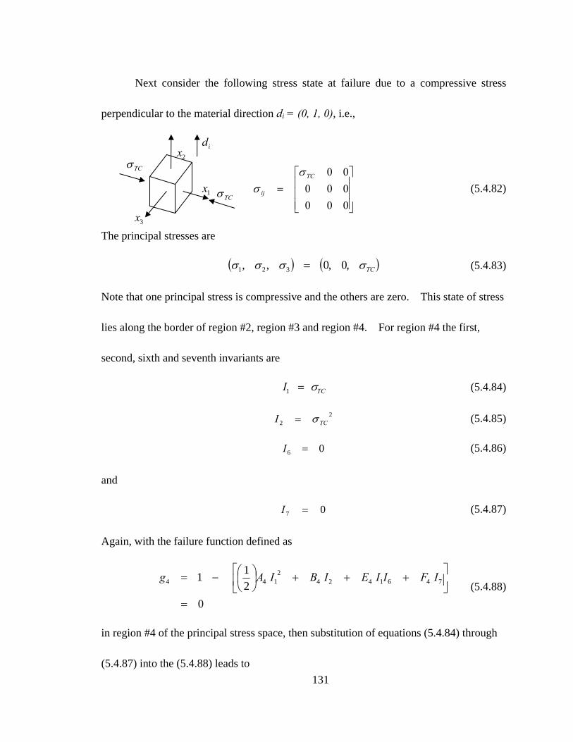
131
Next consider the following stress state at failure due to a compressive stress
perpendicular to the material direction di = (0, 1, 0), i.e.,
000
000
00TC
ij
(5.4.82)
The principal stresses are
TC ,0,0,, 321 (5.4.83)
Note that one principal stress is compressive and the others are zero. This state of stress
lies along the border of region #2, region #3 and region #4. For region #4 the first,
second, sixth and seventh invariants are
TCI 1 (5.4.84)
22 TCI (5.4.85)
06 I (5.4.86)
and
07 I (5.4.87)
Again, with the failure function defined as
0
2
11 7461424
2144
IFIIEIBIAg
(5.4.88)
in region #4 of the principal stress space, then substitution of equations (5.4.84) through
(5.4.87) into the (5.4.88) leads to
1x
2x
3x
id
TC
TC

132
2
42
42
110 TCTC BA (5.4.89)
or
244
1
2
1
TC
BA
(5.4.90)
The unit principal stress vector associated with this state of stress in region #2 is
)0,0,1(2 ia (5.4.91)
thus
000
000
00122
ji aa (5.4.92)
The stress invariants associated with this principal stress vector and state of stress are
TCI 42 (5.4.93)
25
2TCI (5.4.94)
082 I (5.4.95)
and
092 I (5.4.96)
Again, the failure function for stress region #2 has the form
0
2
11
9281272612
52412222
122
IHIIGIFIIE
IDIICIBIAg
(5.4.97)

133
With equations (5.4.84) through (5.4.87) as well as equations (5.4.93) through (5.4.96)
then
2
22
22
22 2
11 TCTCTC DBAg (5.4.98)
or
2222
1
2
1
TC
DBA
(5.4.99)
The unit principal stress vector associated with this state of stress in region #3 is
)0,1,0(3 ia (5.4.100)
thus
000
010
00033
ji aa (5.4.101)
The stress invariants associated with this principal stress vector and state of stress are
043 I (5.4.102)
053 I (5.4.103)
083 I (5.4.104)
and
093 I (5.4.105)
Again, the failure function for stress region #3 has the form
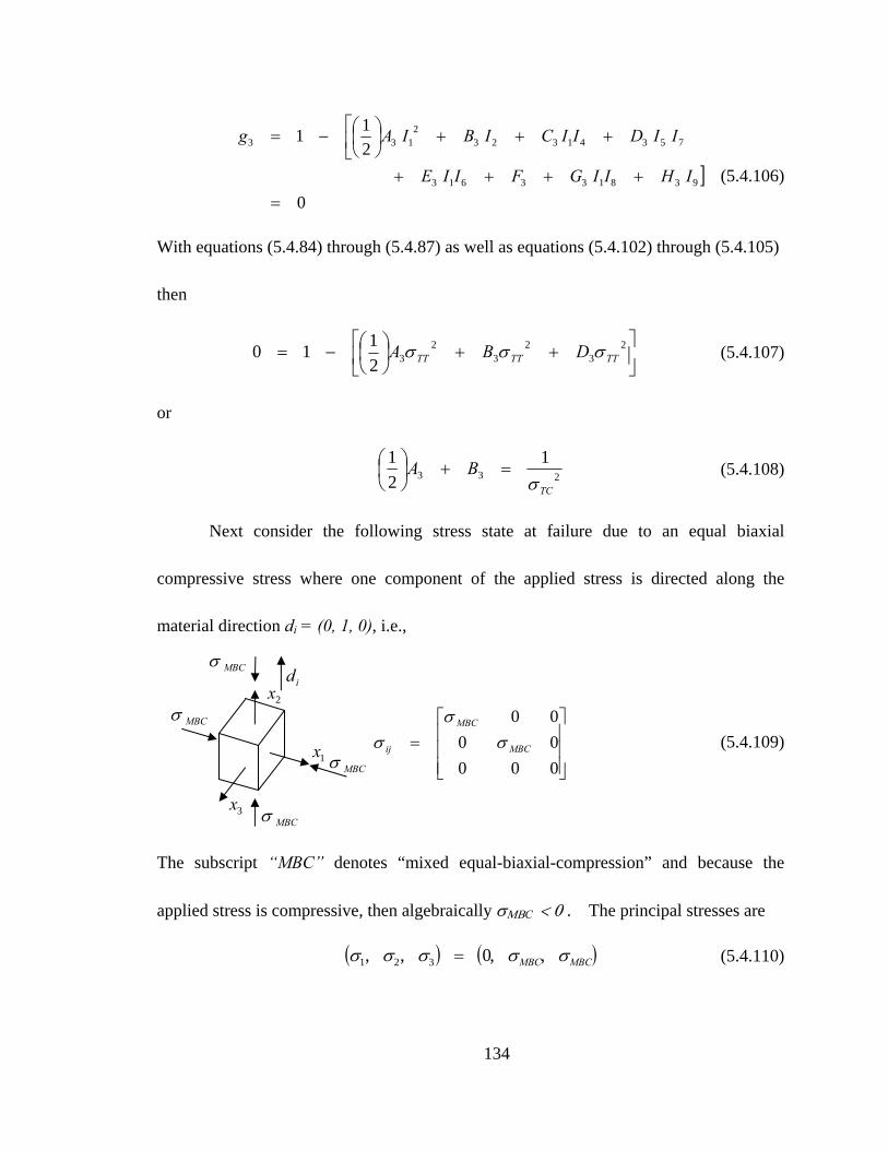
134
0
2
11
938133613
753413232
133
IHIIGFIIE
IIDIICIBIAg
(5.4.106)
With equations (5.4.84) through (5.4.87) as well as equations (5.4.102) through (5.4.105)
then
2
32
32
32
110 TTTTTT DBA (5.4.107)
or
233
1
2
1
TC
BA
(5.4.108)
Next consider the following stress state at failure due to an equal biaxial
compressive stress where one component of the applied stress is directed along the
material direction di = (0, 1, 0), i.e.,
000
00
00
MBC
MBC
ij
(5.4.109)
The subscript “MBC” denotes “mixed equal-biaxial-compression” and because the
applied stress is compressive, then algebraically C . The principal stresses are
MBCMBC ,,0,, 321 (5.4.110)
1x
2x
3x
MBC
id
MBC
MBC
MBC
135
Note that two principal stresses are compressive and the other is zero. This state of
stress lies along the border region #3 and region #4. For stress region #4 the first,
second, sixth and seventh invariants are
MBCI 21 (5.4.111)
22 2 MBCI (5.4.112)
MBCI 6 (5.4.113)
and
27 MBCI (5.4.114)
Again, with the failure function defined as
0
2
11 7461424
2144
IFIIEIBIAg
(5.4.115)
in region #4 of the principal stress space, then substitution of equations (5.4.111) through
(5.4.114) into the (5.4.115) leads to
244
24
24
2
222
110
MBCMBCMBC
MBCMBC
FE
BA
(5.4.116)
or
24444
1222
MBC
FEBA
(5.4.117)
The unit principal stress vector associated with this state of stress in region #3 is
)1,0,0(3 ia (5.4.118)
136
thus
100
000
00033
ji aa (5.4.119)
The stress invariants associated with this principal stress vector and state of stress are
043 I (5.4.120)
053 I (5.4.121)
083 I (5.4.122)
and
093 I (5.4.123)
The failure function for stress region #3 now has the form
0
2
11
938133613
753413232
133
IHIIGFIIE
IIDIICIBIAg
(5.4.124)
With equations (5.4.111) through (5.4.114) as well as equations (5.4.120) through
(5.4.123) then
233
23
23
2
222
110
MBCMBCMBC
MBCMBC
FE
BA
(5.4.125)
or
23333
1222
MBC
FEBA
(5.4.126)
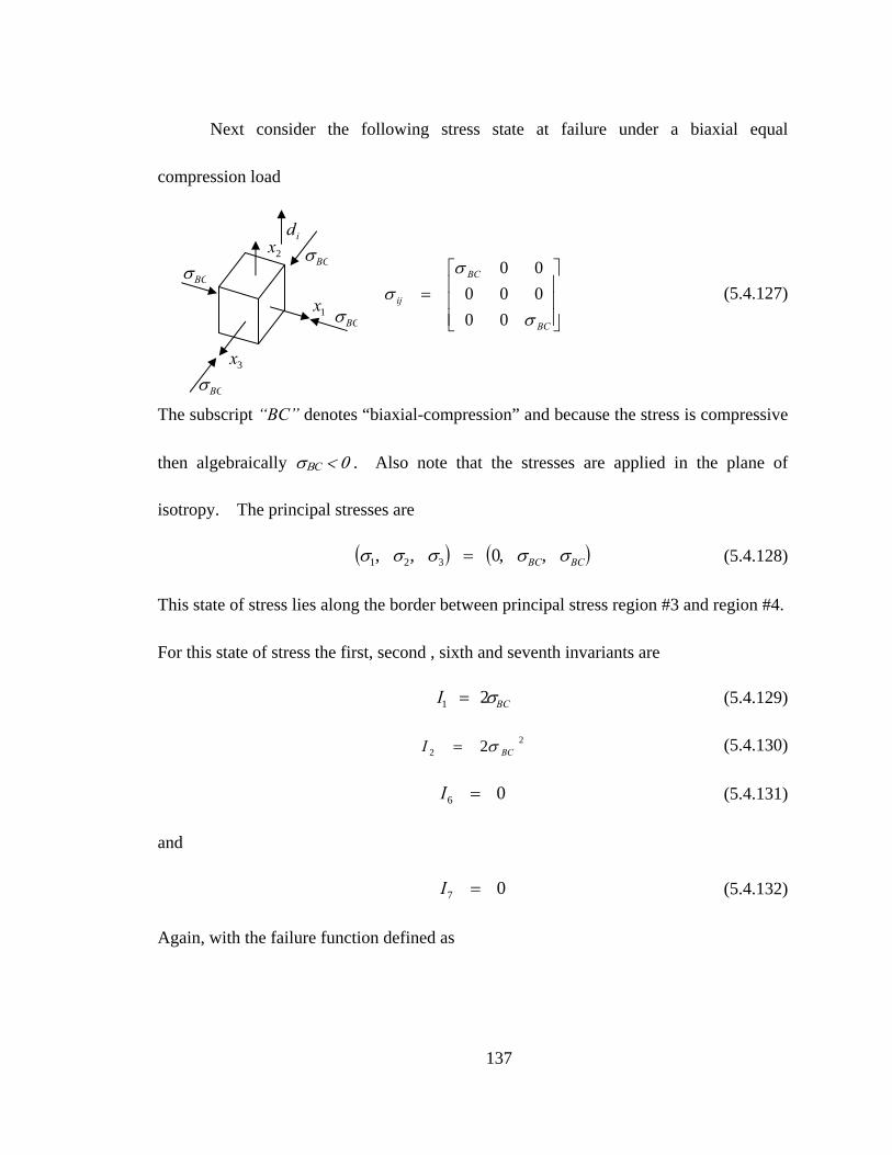
137
Next consider the following stress state at failure under a biaxial equal
compression load
BC
BC
ij
00
000
00
(5.4.127)
The subscript “BC” denotes “biaxial-compression” and because the stress is compressive
then algebraically C. Also note that the stresses are applied in the plane of
isotropy. The principal stresses are
BCBC ,,0,, 321 (5.4.128)
This state of stress lies along the border between principal stress region #3 and region #4.
For this state of stress the first, second , sixth and seventh invariants are
BCI 21 (5.4.129)
22 2 BCI (5.4.130)
06 I (5.4.131)
and
07 I (5.4.132)
Again, with the failure function defined as
1x
2x
3x
BC
BC
id
BC
BC
138
0
2
11 7461424
2144
IFIIEIBIAg
(5.4.133)
in region #4 of the principal stress space, then substitution of equations (5.4.129) through
(5.4.132) into the (5.4.133) leads to
1222
10 2
42
4
BCBC BA (5.4.134)
or
244
122
BC
BA
(5.4.135)
The unit principal stress vector associated with this state of stress in region #3 is
)0,1,0(3 ia (5.4.136)
thus
000
010
00033
ji aa (5.4.137)
The stress invariants associated with this principal stress vector and state of stress are
043 I (5.4.138)
053 I (5.4.139)
083 I (5.4.140)
and
093 I (5.4.141)
The failure function for stress region #3 now has the form
139
0
2
11
938133613
753413232
133
IHIIGFIIE
IIDIICIBIAg
(5.4.142)
With equations (5.4.129) through (5.4.132) as well as equations (5.4.138) through
(5.4.141) then
2
32
3 222
110 BCBC BA (5.4.143)
or
233
122
BC
BA
(5.4.144)
With equations (5.4.9), (5.4.18), (5.4.27), (5.4.36), (5.4.45), (5.4.54), (5.4.63), (5.4.72),
(5.4.81), (5.4.90), (5.4.99), (5.4.108), (5.4.117), (5.4.126), (5.4.135), and (5.4.144) there
are sixteen equations in terms of six strength parameters, i.e.,
YT – tensile strength in the preferred material direction
YC – compressive strength in the preferred material direction
TT – tensile strength in the plane of isotropy
TC – compressive strength in the plane of isotropy
BC – equal biaxial compressive strength in the plane of isotropy
MBC – equal biaxial compressive strength with only one stress component in
the plane of isotropy
140
These equations can be used to extract relationships between the functional constants (A1
through F4) and the mechanical strength parameters listed above. For example,
subtracting equation (5.4.63) from equation (5.4.90) yields
2214
11
TTTC
BB
(5.4.145)
and utilizing equations (5.3.147) and (5.3.148) leads to
2
2214
11
D
BBTTTC
(5.4.146)
In addition, subtracting equation (5.4.9) from equation (5.4.36) yields
221414
11
YTYC
FFBB
(5.4.147)
Furthermore, subtraction equation (5.4.145) from equation (5.4.147) results in
222214
1111
TTTCYTYC
FF
(5.4.148)
and utilizing equations (5.3.150) and (5.3.151) leads to
2
222214
1111
H
FFTTTCYTYC
(5.4.149)
In addition, subtracting equation (5.4.99) from equation (5.4.135) yields
2222424
212222
TCBC
BDBAA
(5.4.150)
Utilizing equations (5.3.146) through (5.3.148) this expression simplifies to

141
224
21
TCBC
A
(5.4.151)
Subtraction of equation (5.4.135) from (5.4.108)
224343
2
122
BCTC
BBAA
(5.4.152)
and utilizing equations (5.3.146) and (5.3.137) leads to
2243
2
12
BCTC
BB
(5.4.153)
Utilizing equation (5.3.146) and subtracting equation (5.4.151) from equation (5.4.63)
yields
2221
1
2
11
TCBCTT
B
(5.4.154)
With equations (5.3.124), (5.3.130), (5.3.137), and (5.3.142), then subtracting equation
(5.4.54) from equation (5.4.117) leads to
22444
11
2
3
YCMBC
EBA
(5.4.155)
Substitution of equations (5.4.151) and (5.4.153) into (5.4.155) yields the following
relationship
22224
1111
TCBCYCMBC
E
(5.4.156)
With equations (5.3.149) and (5.4.150), then subtraction equation (5.4.135) from
equation (5.4.126) results in
142
2244
112
BCMBC
FE
(5.4.157)
Substitution of equation (5.4.156) into (5.4.157) yields
22224
2211
TCYCBCMBC
F
(5.4.158)
Substitution of equation (5.4.158) into (5.4.148) leads to the following
2222221
111111
TTYTTCYCBCMBC
F
(5.4.159)
In summary,
7161121
2111 2
11 IFIIEIBIAg (5.2.1)
9272612
52222
122 2
11
IHIFIIE
IDIBIAg
(5.4.160)
933613
753232
133 2
11
IHFIIE
IIDIBIAg
(5.4.161)
and
7461424
2144 2
11 IFIIEIBIAg (5.2.43)
where
224321
12
BCTC
AAAA
(5.4.162)
22221
2
111
BCTCTT
BB
(5.4.163)

143
2243
2
12
BCTC
BB
(5.4.164)
2232
11
TCTT
DD
(5.4.165)
2222
4321
1111
MBCYCBCTC
EEEE
(5.4.166)
222
22221
111
111
MBCYCYT
BCTCTT
FF
(5.4.167)
222243
1212
MBCYCBCTC
FF
(5.4.168)
and
222232
1111
YCYTTCTT
HH
(5.4.169)
Equations (5.4.160) and (5.4.169) along with equations (5.2.1) and (5.2.43) is a complete
statement of the anisotropic failure functions in a regions of the stress space.
The anisotropic failure criterion is projection onto the 11 – 22 stress space in
Figure 5.4.1. The strength parameters were for the most part extracted from the data
found in Burchell et al. (2007), i.e., TT =10.48 MPa, YT =15.93 MPa and YC =52.93
MPa (see Table 2.2). These are average or mean strength values. The other three
strength parameters YT, YC, BC and MBC were estimated. Values for the strength
parameters listed above are given in the figure caption. Note the agreement with the
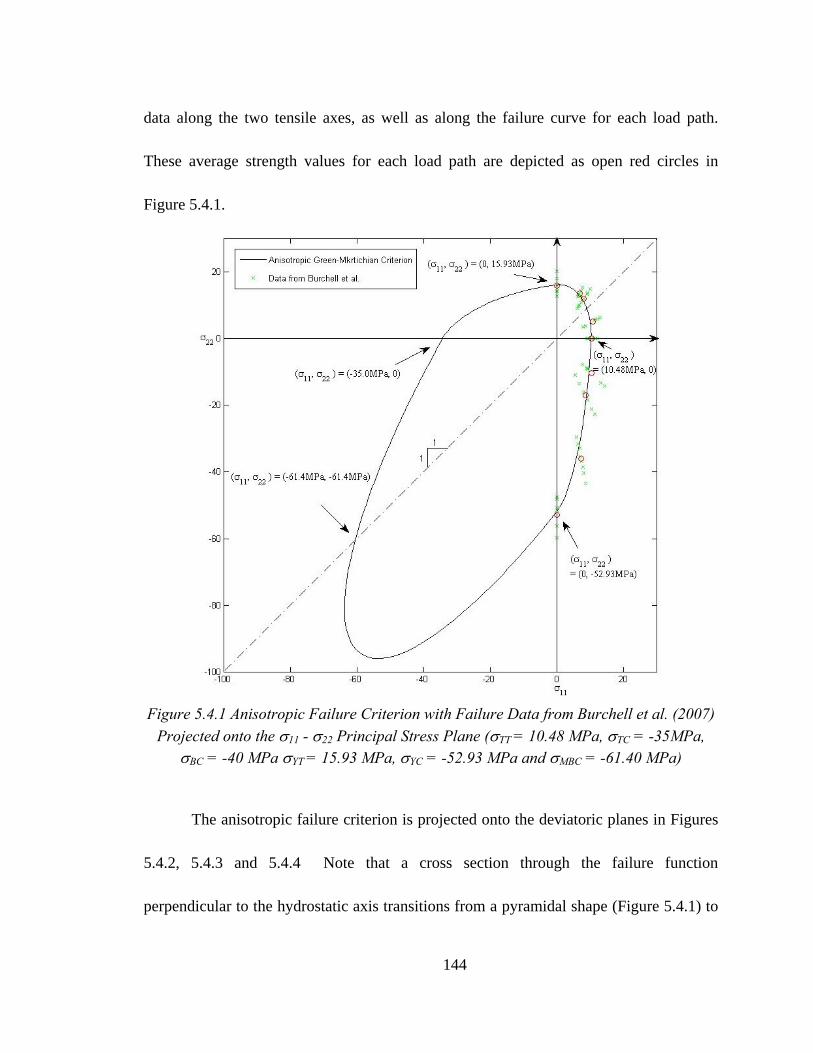
144
data along the two tensile axes, as well as along the failure curve for each load path.
These average strength values for each load path are depicted as open red circles in
Figure 5.4.1.
Figure 5.4.1 Anisotropic Failure Criterion with Failure Data from Burchell et al. (2007)
Projected onto the 11 - 22 Principal Stress Plane (TT = 10.48 MPa, TC = -35MPa, BC = -40 MPaYT = 15.93 MPa, YC = -52.93 MPa and MBC = -61.40 MPa)
The anisotropic failure criterion is projected onto the deviatoric planes in Figures
5.4.2, 5.4.3 and 5.4.4 Note that a cross section through the failure function
perpendicular to the hydrostatic axis transitions from a pyramidal shape (Figure 5.4.1) to

145
a circular shape (Figure 5.4.2) with an increasing value of the stress invariant I1. This
suggests that the apex of the failure function presented in a full Haigh-Westergaard stress
space is blunt, i.e., quite rounded for this particular criterion.
Figure 5.4.2 Anisotropic Failure Criterion with Failure Data from Burchell et al. (2007)
Projected onto (= 6.05 MPa) Parallel to the -plane(TT = 10.48 MPa, TC = -35MPa, BC = -40 MPaYT = 15.93 MPa, YC = -52.93 MPa,
MBC = -61.40 MPa)

146
Figure 5.4.3 Anisotropic Failure Criterion with Failure Data from Burchell et al. (2007)
Projected onto (= 9.02 MPa) Parallel to the -plane(TT = 10.48 MPa, TC = -35MPa, BC = -40 MPaYT = 15.93 MPa, YC = -52.93 MPa, MBC = -61.40 MPa)
Figure 5.4.4 Anisotropic Failure Criterion with Burchell’s (2007) Failure Data Projected onto (= -30.20) Parallel to the -plane(TT = 10.48 MPa, TC = -35MPa,
BC = -40 MPaYT = 15.93 MPa, YC = -52.93 MPa, MBC = -61.40 MPa)
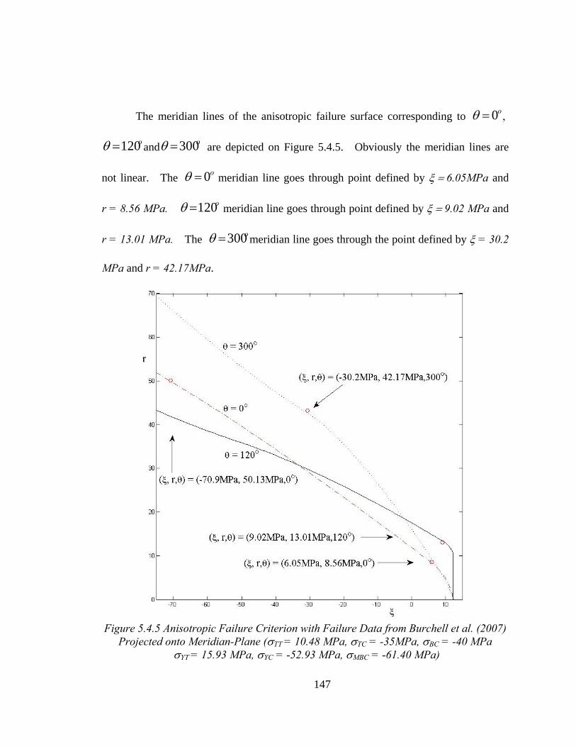
147
The meridian lines of the anisotropic failure surface corresponding to o0
o120 ando300 are depicted on Figure 5.4.5. Obviously the meridian lines are
not linear. The o0 meridian line goes through point defined by 6.05MPa and
r = 8.56 MPa. o120 meridian line goes through point defined by 9.02 MPa and
r = 13.01 MPa. The o300 meridian line goes through the point defined by = 30.2
MPa and r = 42.17MPa.
Figure 5.4.5 Anisotropic Failure Criterion with Failure Data from Burchell et al. (2007)
Projected onto Meridian-Plane (TT = 10.48 MPa, TC = -35MPa, BC = -40 MPa YT = 15.93 MPa, YC = -52.93 MPa, MBC = -61.40 MPa)

148
As the value of the I1 stress invariant associated with the hydrostatic stress
increases in the negative direction, failure surfaces perpendicular to the hydrostatic stress
line become circular again. The model suggests that as hydrostatic compression stress
increases the difference between tensile strength and compressive strength diminishes
and approach each other asymptotically. This is a material behavior that should be
verified experimentally in a manner similar to Bridgman’s (1953) bend bar experiments
conducted in hyperbaric chambers on cast metal alloys. Balzer (1998) provides an
excellent overview of Bridgman’s (1953) experimental efforts, as well as others and their
accomplishments in the field of high pressure testing.
149
CHAPTER VI
MATERIAL STRENGTH AS A RANDOM VARIABLE
All parameters in an engineering design can be treated as random variables. For
example material strength, loads applied to the component, geometric dimensions, as well
as the stiffness of the material utilized can all exhibit significant levels of variability.
However, the assumption is made for graphite that the variability in material strength far
exceeds the variability one would see in the other design parameters. This seems
reasonable since the strength of graphite material can vary by 50% or more. Earthquake
loads can be the exception to this exclusion of all other design parameters, although
including load design parameters as well as resistance design parameters other than
material strength as random variables is easily accomplished.
A failure function characterizes a limit state through its formulation and the design
parameters that the function is dependent on. Although one can easily pose limit states
for fracture (e.g., failure assessment diagrams), fatigue life or service issues relating to
structural deformations in this effort all design parameters here are related to strength.
150
In the previous chapters a number of failure criteria, i.e., limit state functions, were
highlighted and discussed. The goal in examining the various failure criteria is the
development of a phenomenological, stress based function that captures the fundamental
strength behavior of nuclear graphite exhibited through the data from Burchell et al.
(2007). This behavior includes different failure behavior in tension and compression, as
well as the anisotropy exhibited along different load paths. In the last chapter the
isotropic failure criterion was extended to transversely anisotropic behavior through the
use of tensorial invariants that include material direction tensors. Other types of
anisotropies can be considered using this approach, e.g., orthotropic strength behavior.
The phenomenological failure criteria outlined in the previous chapters were all posed as
deterministic limit states. The last aspect of material behavior that is explored in this
chapter requires consideration is how to account for the variability in the strength
parameters.
The multiaxial graphite data from Burchell et al. (2007) has been cited throughout
this work and one cannot help but see that the strength of graphite material is essentially
stochastic along various load paths depicted in Figure 2.4.1. With the amount of
variation exhibited by the graphite data in that figure and based on graphite failure data
available throughout the literature, it is not difficult to identify graphite strength as a
random variable. The strength parameters identified in the last chapter for the
anisotropic failure criterion, i.e., YT (tensile strength in the preferred material direction),
151
YC (compressive strength in the preferred material direction), TT (tensile strength in the
plane of isotropy), TC (compressive strength in the plane of isotropy), BC (equal biaxial
compressive strength in the plane of isotropy), and MBC (equal biaxial compressive
strength with only one stress component in the plane of isotropy) are all treated as
random variables based on evidence found within the data from Burchell et al. (2007).
The assumption is made that these strength parameters are statistically independent
random variables. The veracity of this assumption will be left for future efforts.
Methods available to interrogate this issue will be outlined in the summary chapter.
Another assumption is made relative to the particular probability density function used to
represent the strength random variables. Here the two parameter Weibull distribution is
adopted for all random strength parameters. Again there are methods to test the validity
of that assumption. But since this is a proof of concept effort, those sort of goodness of
fit tests are left to others to pursue.
In general, the strength parameters associated with the load paths from the data
found in Burchell et al. (2007) can be assembled into an k-dimensional vector, i.e.,
kYYYY ,,, 21 (6.1)
and a limit state function can be defined in general terms as
0, ijyg (6.2)
Here y represents a vector of realizations of the random variables identified by the
strength parameters in the previous chapter and ij is the applied Cauchy stress tensor.

152
This last expression defines a surface in an k-dimensional stress space. The limit state
function for the anisotropic failure criterion is adopted for graphite and this criterion
would have the following multipart formulation in the principal (Haigh-Westergaard)
stress space
Region #1: 0321
0
2
11 7161121
2111
IFIIEIBIAg
(6.3)
Region #2: 321 0
0
2
11
9281272612
52412222
122
IHIIGIFIIE
IDIICIBIAg
(6.4)
Region #3: 321 0
0
2
11
938133613
753413232
133
IHIIGFIIE
IIDIICIBIAg
(6.5)
Region #4: 3210
0
2
11 7461424
2144
IFIIEIBIAg
(6.6)
The various constants defined in the previous chapter (identified above as A through F
with subscripts) are no longer constants since they are functions of strength parameters.
153
Hence these parameters are now considered composite random variables. In essence
they are functions of random variables
The fundamental issue of no longer treating material strength as a deterministic,
single valued parameter complicates the issue of how to interpret failure at a point
through the state of stress at that point. If strength is treated as a random variable, how
does that affect the approach the design engineer takes in assessing whether a component
performs its intended function properly or not? A different design philosophy must be
adopted in this situation where a simple fail/no fail interpretation is replaced with an
equivalent stochastic decision process that predicts the probability of component failure.
In general, the reliability (probability of failure) is computed based on the
expression
0, ijygyProbabilit R (6.7)
This calculation is made for a unit volume of a point of material with a homogenous state
of stress. To calculate the reliability of an element the joint density function must be
integrated over the “safe” region of the design space which is defined by the limit state
function. This integration takes the form
BCCTBCCT
yg
dydydyyyyij
,,0,
R (6.8)
for the isotropic formulation of the limit state function for graphite. Here the three
random strength parameters YT, YC and YBC are associated with the deterministic strength

154
parameters T, C and BC. Again, the lower case letters associated with the random
strength parameters are realizations of the random strengths. In addition
MBCYCYTBCTCTTMBCYCYTBCTCTT
yg
dydydydydydyyyyyyyij
,,,,,0,
R (6.9)
serves as the generic integration for the anisotropic limit state function. Here is the
joint density function of material strength parameters. Sun and Yamada (1978) as well
as Wetherhold (1983) point out that the integration defined by either equations (6.8) and
(6.9) yields the reliability of a unit volume based on the state of stress at a point.
However, closed form solutions for these types of reliability expressions are not
available. Palko (1992) and Hu (1994) illustrate how the integration in these
expressions can be executed using techniques based on Monte Carlo simulation. These
techniques are deployed here.
Having identified graphite strength as a random variable the next step is selecting
an appropriate probability density function to characterize each strength random variable.
In general material strength should be characterized by an extreme value distribution. In
structural design one is always interested in the extreme minimum values in a random
variable representing strength, i.e., a resistance random variable. If load is similarly
characterized as a random variable the design engineer would be cognizant of the
extreme maximum values representing of this variable. Weibull (1939) formulated a
probability density function with two parameters to characterize a type III extreme value

155
distribution. If a single strength parameter is considered then is equal to one and the
following notation can be adopted
Y
YY
1 (6.10)
The cumulative probability density function for a two parameter Weibull distribution is
given by the expression
m
YY
y
FF
exp1 (6.11)
where y is the realization of the strength random variable (usually an applied uniaxial
stress, ) m is the Weibull modulus and is known as the scale parameter. This
equation can be linearized by taking the natural logarithm of both sides of the expression
twice, i.e.,
lnln1
1lnln mC
FY
(6.12)
where
m
C
1
ln (6.13)
The format of equation (6.12) lends itself to an easy graphical format, an example of
which is given in Figure 6.1. Here values for the Weibull parameters were arbitrarily
assumed (see the figure caption). These linearized probability plots are used extensively
in this chapter to explain the fundamentals of the numerical integration techniques used
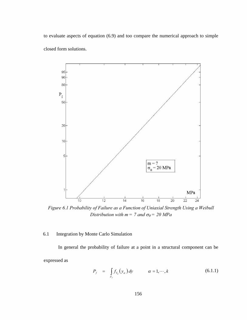
156
to evaluate aspects of equation (6.9) and too compare the numerical approach to simple
closed form solutions.
Figure 6.1 Probability of Failure as a Function of Uniaxial Strength Using a Weibull
Distribution with m = 7 and = 20 MPa
6.1 Integration by Monte Carlo Simulation
In general the probability of failure at a point in a structural component can be
expressed as
f
kdyyfP Yf
,,1 (6.1.1)
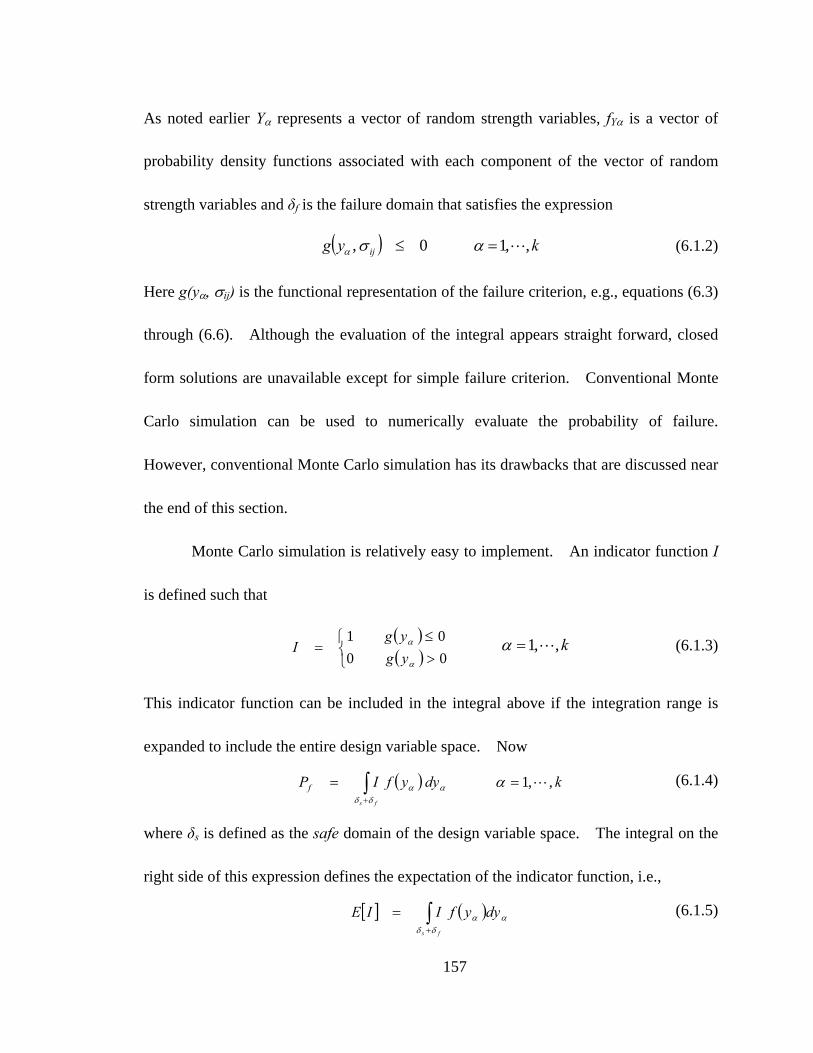
157
As noted earlier Y represents a vector of random strength variables, fY is a vector of
probability density functions associated with each component of the vector of random
strength variables and δf is the failure domain that satisfies the expression
kyg ij ,,10, (6.1.2)
Here g(yij) is the functional representation of the failure criterion, e.g., equations (6.3)
through (6.6). Although the evaluation of the integral appears straight forward, closed
form solutions are unavailable except for simple failure criterion. Conventional Monte
Carlo simulation can be used to numerically evaluate the probability of failure.
However, conventional Monte Carlo simulation has its drawbacks that are discussed near
the end of this section.
Monte Carlo simulation is relatively easy to implement. An indicator function I
is defined such that
00
01
yg
ygI k,,1 (6.1.3)
This indicator function can be included in the integral above if the integration range is
expanded to include the entire design variable space. Now
kdyyfIPfs
f ,,1
(6.1.4)
where δs is defined as the safe domain of the design variable space. The integral on the
right side of this expression defines the expectation of the indicator function, i.e.,
fs
dyyfIIE
(6.1.5)
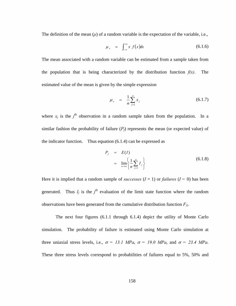
158
The definition of the mean (μ) of a random variable is the expectation of the variable, i.e.,
dxxfxx
(6.1.6)
The mean associated with a random variable can be estimated from a sample taken from
the population that is being characterized by the distribution function f(x). The
estimated value of the mean is given by the simple expression
n
jjx x
n 1
1 (6.1.7)
where xj is the jth observation in a random sample taken from the population. In a
similar fashion the probability of failure (Pf) represents the mean (or expected value) of
the indicator function. Thus equation (6.1.4) can be expressed as
n
jj
n
f
In
IEP
1
1lim
)(
(6.1.8)
Here it is implied that a random sample of successes (I = 1) or failures (I = 0) has been
generated. Thus Ij is the jth evaluation of the limit state function where the random
observations have been generated from the cumulative distribution function FX.
The next four figures (6.1.1 through 6.1.4) depict the utility of Monte Carlo
simulation. The probability of failure is estimated using Monte Carlo simulation at
three uniaxial stress levels, i.e., = 13.1 MPa, = 19.0 MPa, and = 23.4 MPa.
These three stress levels correspond to probabilities of failures equal to 5%, 50% and

159
95% for a uniaxial strength random variable characterized by a two parameter Weibull
distribution with m = 7 and = 20 MPa.
Figure 6.1.1 Estimates from Monte Carlo Simulations (n=100) at Low (5%), Medium (50%) and High (95%) Levels of Probability of Failure Compared to the Underlying
Weibull Population Distribution (m = 7 and = 20 MPa)
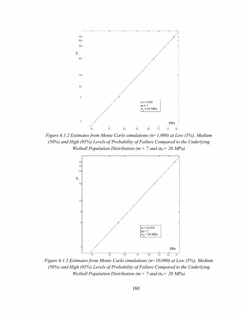
160
Figure 6.1.2 Estimates from Monte Carlo simulations (n=1,000) at Low (5%), Medium (50%) and High (95%) Levels of Probability of Failure Compared to the Underlying
Weibull Population Distribution (m = 7 and = 20 MPa)
Figure 6.1.3 Estimates from Monte Carlo simulations (n=10,000) at Low (5%), Medium
(50%) and High (95%) Levels of Probability of Failure Compared to the Underlying
Weibull Population Distribution (m = 7 and = 20 MPa)

161
The open circles in all four figures represent estimates of the probability of failure
using conventional Monte Carlo simulation. The straight line in each figure represents
the parent populations the sample strengths are being extracted from. Several
observations can be made. First the estimate of the probability of failure at the 5% level
is not good until the number of samples is increased to 10,000 (see figure 6.1.3). In
addition, the estimate of the probability of failure is quite good for all sample sizes at the
95% probability of failure level. This second observation should not be considered
meritorious for conventional Monte Carlo simulation since most engineering designs
based on probabilistic methods will strive for the regions of low probability of failures.
This loss of fidelity of the conventional Monte Carlo simulation approach in the low
probability of failure regimes is a distinct disadvantage in using this numerical method to
estimate the integral in equation 6.9.

162
Figure 6.1.4 Estimates from Monte Carlo simulations (n=100,000) at Low (5%), Medium (50%) and High (95%) Levels of Probability of Failure Compared to the Underlying
Weibull Population Distribution (m = 7 and = 20 MPa)
To a certain extent the loss of fidelity in the low probability of failure regimes can
be rectified by increasing the number of simulations (see figure 6.1.4). However,
depending on how low the required design failure rate is, this issue can still be a problem
as evidenced by the probability of failure estimates presented in figure 6.1.5. Here
values of probability of failure are estimated for uniaxial stress levels of 3.86 MPa,
5.37 MPa and 7.46 MPa for the same population sampled in the previous four figures.
These values of stress correspond to exact values of probability of failure in the parent
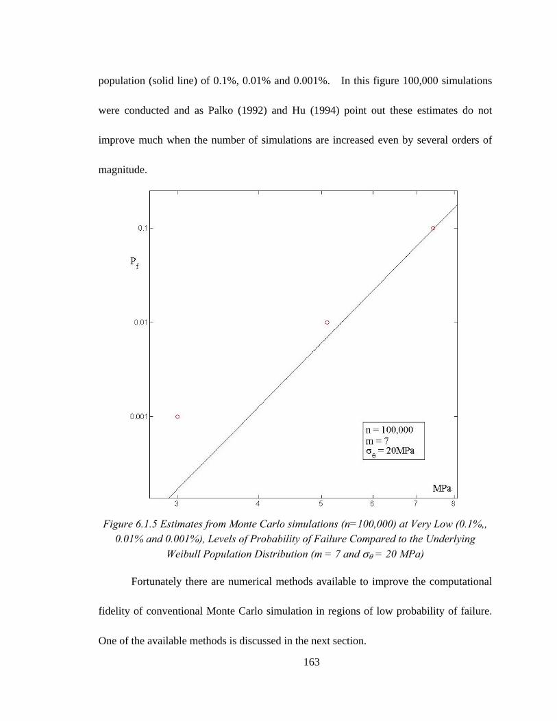
163
population (solid line) of 0.1%, 0.01% and 0.001%. In this figure 100,000 simulations
were conducted and as Palko (1992) and Hu (1994) point out these estimates do not
improve much when the number of simulations are increased even by several orders of
magnitude.
Figure 6.1.5 Estimates from Monte Carlo simulations (n=100,000) at Very Low (0.1%,, 0.01% and 0.001%), Levels of Probability of Failure Compared to the Underlying
Weibull Population Distribution (m = 7 and = 20 MPa)
Fortunately there are numerical methods available to improve the computational
fidelity of conventional Monte Carlo simulation in regions of low probability of failure.
One of the available methods is discussed in the next section.
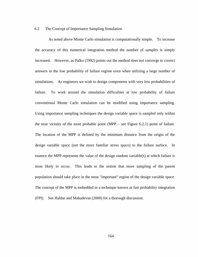
164
6.2 The Concept of Importance Sampling Simulation
As noted above Monte Carlo simulation is computationally simple. To increase
the accuracy of this numerical integration method the number of samples is simply
increased. However, as Palko (1992) points out the method does not converge to correct
answers in the low probability of failure regime even when utilizing a large number of
simulations. As engineers we wish to design components with very low probabilities of
failure. To work around the simulation difficulties at low probability of failure
conventional Monte Carlo simulation can be modified using importance sampling.
Using importance sampling techniques the design variable space is sampled only within
the near vicinity of the most probable point (MPP – see Figure 6.2.1) point of failure.
The location of the MPP is defined by the minimum distance from the origin of the
design variable space (not the more familiar stress space) to the failure surface. In
essence the MPP represents the value of the design random variable(s) at which failure is
most likely to occur. This leads to the notion that more sampling of the parent
population should take place in the most "important" region of the design variable space.
The concept of the MPP is embedded in a technique known as fast probability integration
(FPI). See Haldar and Mahadevan (2000) for a thorough discussion.
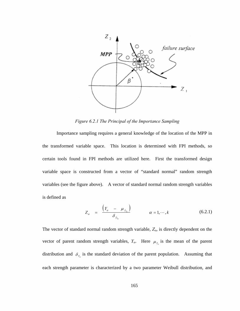
165
Figure 6.2.1 The Principal of the Importance Sampling
Importance sampling requires a general knowledge of the location of the MPP in
the transformed variable space. This location is determined with FPI methods, so
certain tools found in FPI methods are utilized here. First the transformed design
variable space is constructed from a vector of “standard normal” random strength
variables (see the figure above). A vector of standard normal random strength variables
is defined as
kY
ZY
Y
f
f,,1
(6.2.1)
The vector of standard normal random strength variable, Zα, is directly dependent on the
vector of parent random strength variables, Yα. Here
Y is the mean of the parent
distribution and
Y is the standard deviation of the parent population. Assuming that
each strength parameter is characterized by a two parameter Weibull distribution, and

166
with knowledge of the Weibull distribution parameters and m for each strength
parameter, then the expression
kmYf
,,11
1
(6.2.2)
is used to compute the mean for each random strength variable (note that is the gamma
function). Note that vectors of distribution parameters, i.e., m and ( are required,
each pair corresponding to a particular strength random variable. The next expression
kmmYf
,,11
12
1
2
2
(6.2.3)
is used to calculate the standard deviation for each random strength variable. For
completeness the following expression stipulates the probability density function for a
vector of random strength variables characterized by a two parameter Weibull
distribution
kyym
yf
mm
Y ,,1exp
1
(6.2.4)
The subscript is identified in various ways for each of the random strength variables
adopted with a failure criterion, i.e., “T”, “C” and “BC” (k=3) for the isotropic version of
the failure function. For the anisotropic version is identified with “YT”, “YC”, “TT”,
“TC”, “BC” and “MBC” (k=6). Assuming the strength random variables are
statistically independent, then a joint probability density function can be formulated using
the expression
167
kyfyfk
Y ,,11
(6.2.5)
This notation is used momentarily.
If the limit state function is linearized and the design random variables can be
transformed to standard normal variables then the reliability index is used to locate the
MPP – see Hu (1994), Wetherhold and Ucci (1994) as well as Haldar and Mahadevan
(2000). However, determining the exact location of the MPP is not necessary to
implement importance sampling – just a knowledge of the general vicinity of the MPP.
An advantage of importance sampling relative to FPI methods is that importance
sampling alleviates a potential non-conservative numerical error associated with FPI
methods. The limit state function in this work is by no means a linear function in terms
of the design random variables and when using FPI techniques the limit state function is
approximated by a hyper-plane at the MPP. Wetherhold and Ucci (1994) point out that
a planar approximation can yield non-conservative results depending on the curvature of
the limit state function at the MPP. Since importance sampling does not depend on this
curvature, it effectively avoids this potential non-conservative numerical error.
For importance sampling equation (6.1.4) is rearranged such that
kdyykyk
yfIP
ff
f ,,1
(6.2.6)
A new joint probability density function, k(y), is introduced in the last expression. This
function serves as a weighting function that forces the simulation process to sample in the
168
near vicinity of the MPP. This joint probability density function is formulated using the
following expression
kykykn
Y ,,11
(6.2.7)
Although the procedure does not limit the type of probability distribution one can use for
each individual random variable (the individual probability density function for each
random variable is identified by ) a standard normal distribution is assumed here for
simplicity, i.e.,
ky
ykk
Y
Y
Y k
k
k
YY
,,12
1exp
2
12
(6.2.8)
An individual importance sampling function should have the following properties:
1. > 0 whenever 0yf ;
2. should be closely proportional to yf , i.e., the importance sampling
function should roughly have the same shape as the parent strength distribution;
and
3. the importance sampling function should be selected such that values can be
easily simulated from the function and the cumulative density function can be
readily computed from the simulated value.
For demonstration purposes the standard normal distribution identified in equation (6.2.8)
was selected. This importance sampling function meets the three properties identified
Yk
Yk
Yk
Yk
169
above. Results for multiaxial simulations indicate that while the form of the function is
appropriate, there is future efforts needed to better define how the variance (standard
deviation) is computed. Note that
YY fk (6.2.9)
and
YY fk (6.2.10)
The mean associated with the standard normal probability density function is given by
the following expression
kz xfxfkY,,1)()(
(6.2.11)
The parameters xf and xf are the mean and standard deviation associated with the
actual probability distribution function that characterizes the random strength variable,
i.e., the parent distribution fX. Earlier the parent distribution for all the strength random
variables was assumed to be a two parameter Weibull distribution and the parameters
xf and xf are identified by equations 6.2.2 and 6.2.3. The standard deviation of
the probability density function is chosen in such a way that the sampling region is
weighted towards the near vicinity of the MPP. Here an approach suggested by
Melchers (1989) is adopted where
kxfxf
k
kY
Y,,131 )(
)(
(6.2.12)
Yk
Yk
170
As will be seen in the multiaxial simulations this approach for computing the standard
deviation needs further optimization.
Given equation 6.2.5, the function serves as the parent probability density
function for a transformed indicator function defined as
kyk
yfII ,,1ˆ
(6.2.13)
Equation (6.2.5) can be expressed as a Riemann sum, i.e.,
n
jj
n
n
jj
n
f
In
yk
yfI
n
IEP
1
1
ˆ1lim
1lim
(6.2.14)
During a given simulation a separate random number is generated (the jth random
number) for each random strength variable and a realization for each of the random
strength variables (Y)j is computed using the inverse of which is the cumulative
distribution function corresponding to . These realizations are used to compute
realizations of Zas well as individual values of , and the limit state function
g(y). The limit state function is dependent on the applied stress state, and the
evaluation of g(y) given the realization of the random variables (Y)j will once again
yield a value of zero or one for the indicator function I in equation 6.2.11. Once the
joint probability functions f(y) and k(y) are formulated the transformed indicator
function is then computed from the same equation. This completes a simulation for the
Yk
YK
Yk
Yk Yf

171
jth iteration and the process is repeated n times. A mean is computed for the transformed
indicator function after n iterations. This mean is an approximation of the probability of
failure given the applied stress state and the statistical information associated with each
strength random variable.
For a low probability of failure the main contribution to Pf will come from regions
near the MPP. The reader is directed to Figure 3.7 in Hu (1994). This region will also
correspond to the tail of the joint probability distribution function of the design strength
random variables. Harbitz (1986) has shown that restricting the sampling domain in the
design variable space to the tail of the joint probability distribution function produces a
remarkable increase in efficiency in comparison to conventional Monte Carlo techniques.
That efficiency is reproduced here.
Harbitz (1986) demonstrated that the number of simulations necessary to achieve
the same order of accuracy obtained from conventional Monte Carlo methods is reduced
by a factor of
21
1
(6.2.15)
where Γα is the chi-square distribution with degrees of freedom, and * is less than or
equal to the actual the reliability index for a given design problem. The degrees of
freedom correspond to the number of design variables included in the limit state function.
In essence, Harbitz (1986) reasoned that random design variables are being sampled from

172
a truncated distribution function. This corresponds to sampling from the actual
probability distribution function, however the sampling domain is restricted to regions
outside a sphere defined in the design variable space (see Figure 6.2.1). The center of
the sphere is located at the origin of the transformed design variable space, and the radius
of the sphere is equal to *. Proof of Harbitz (1986) argument follows from the
interpretation of this geometrical concept. Elements of the FPI method is utilized to
obtain approximate Z values in order to establish a general location of the MPP. For
two random variables the location of the MPP is given by the expression
2122
21 zz (6.2.16)
where is the reliability index. Three or more random variables would be a simple
extension of this geometric concept.
The benefits of utilizing importance sampling can be seen in figure 6.2.2 and
especially in figure 6.2.3. Figure 6.2.2 depicts the result from simple Monte Carlo
simulation with 100 iterations (the open box) at uniaxial stress levels that correspond to
the 5%, 50% and 95% levels of failure probability. Four points are depicted at the same
levels of probability of failure. These points represent importance sampling with 100,
1,000, 10,000 and 100,000 iterations. The improvement in the low region of probability
of failure, the region engineers wish to design in, is obvious with only 100 iterations.
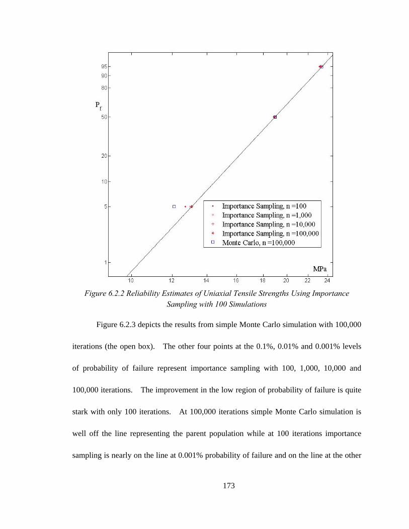
173
Figure 6.2.2 Reliability Estimates of Uniaxial Tensile Strengths Using Importance
Sampling with 100 Simulations
Figure 6.2.3 depicts the results from simple Monte Carlo simulation with 100,000
iterations (the open box). The other four points at the 0.1%, 0.01% and 0.001% levels
of probability of failure represent importance sampling with 100, 1,000, 10,000 and
100,000 iterations. The improvement in the low region of probability of failure is quite
stark with only 100 iterations. At 100,000 iterations simple Monte Carlo simulation is
well off the line representing the parent population while at 100 iterations importance
sampling is nearly on the line at 0.001% probability of failure and on the line at the other

174
two probability of failure. In essence increasing the iterations above 100 the level does
not greatly improve the prediction relative to the parent population. Here is the
advantage of conducting Monte Carlo simulation with importance sampling – a
numerical savings by incurred by dramatically decreasing the number of simulations
required to produce high quality results.
Figure 6.2.3 Reliability Estimates of Uniaxial Tensile Strengths Using Importance
Sampling with 1,000 Simulations
175
6.3 Isotropic Limit State Function – Importance Sampling
The concept of importance sampling is first applied to the isotropic form of the
limit state function. The tensile strength design variable (YT), compressive strength
design variable (YC) and the biaxial compressive strength design variable (YBC) are
characterized by the two-parameter Weibull distributions. To begin the method the
approximate location of the MPP must be determined. Methods to locate the MPP can
be found in Haldar and Mahadevan (2000) as well as Hu (1994). The location of the
MPP is determined through realizations of standard normal variables ZT, ZC and ZBC.
With these realizations serving as the components of a vector, the MPP is located by this
vector. The information regarding the MPP establishes the means for the importance
sampling density functions TYk ,
CYk andBCYk . The importance sampling density functions
facilitate obtaining samples in the near vicinity of the MPP through simulation. Once
the means TYk ,
CYk and BCYk for the importance sampling density functions are
computed using equation (6.2.11) then the values TYTY fk ,
CYCY fk and
BCYBCY fk are established using equation (6.2.12). These are the variances of the
importance sampling density functions and not the variances of the random strength
density functions. Use of equations (6.2.11) and (6.2.12) require the knowledge of the
means from the parent Weibull strength distributions, i.e., TYf
, CYf
and BCYf
as well
as the standard deviations of the parent Weibull strength distributions, i.e., TYf
, CYf
and
CYf . These are assumed known.

176
Once the means and standard deviations are obtained for each importance
sampling density function the next step requires three separate and distinct random
numbers between zero and one. These random numbers serve as values for TYK in the
expression
11
2 2YT
T
YT
T k
Y T
k
yK y erf
(6.3.1)
as well asCYK in the expression
11
2 2YC
C
YC
C k
Y C
k
yK y erf
(6.3.2)
andBCYK in the expression
11
2 2YBC
BC
YBC
BC k
Y BC
k
yK y erf
(6.3.3)
Here “erf” is the error function. The only unknowns in these expressions are the
realizations of the random strength variables YT, YC and YBC. The last three expressions
are solved for these realizations.
Having realizations Ty , Cy and BCy along with means TYk ,
CYk and BCYk
as well as variances TYk ,
CYk and CYk then values of the importance sampling
probability density function
2
2
1exp
2
1
TY
TY
TY
T
k
kT
k
TY
yyk
(6.3.4)
the importance sampling probability density function

177
2
2
1exp
2
1
C
CY
CY
C
k
kC
k
CY
yyk
(6.3.5)
and the Importance sampling probability density function
2
2
1exp
2
1
BC
BCY
BCY
BC
k
kBC
k
BCY
yyk
(6.3.6)
can be computed. The value of the joint importance sampling probability function for the
jth simulation is then ascertained using
jBCYjCYjTYBCCTj ykykykYYYk
BCCT,, (6.3.6)
This joint importance probability sampling function is presumed centered over the MPP.
Realizations for the random strength variables YT, YC and YBC along with Weibull
parameter (m, ) for each random strength variable are then used to evaluate the
probability of density function
TT
T
m
T
T
m
T
T
T
TTY
yymyf
exp
1
(6.3.7)
as well as
CC
C
m
C
C
m
C
C
C
CCY
yymyf
exp
1
(6.3.8)
and
BCBC
BC
m
BC
BC
m
BC
BC
BC
BCBCY
yymyf
exp
1
(6.3.9)
respectively. A numerical value for the joint probability density
jBCYjCYjTYBCCTj yfyfyfYYYf
BCCT,, (6.3.10)
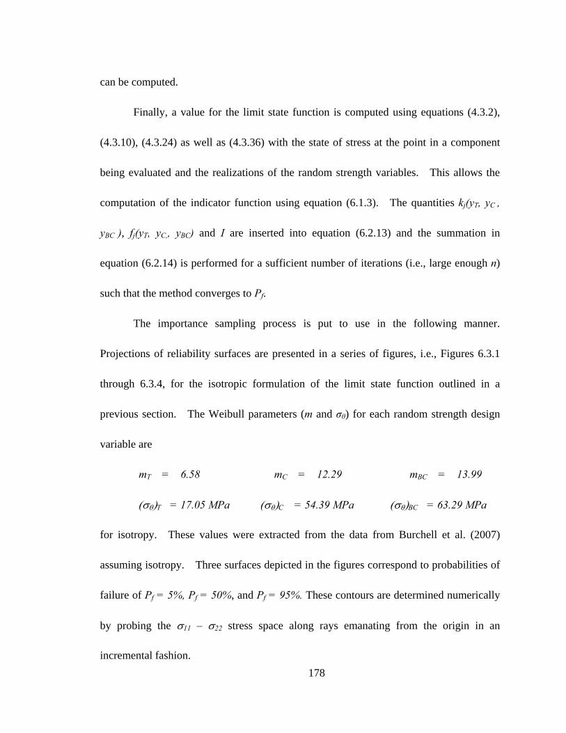
178
can be computed.
Finally, a value for the limit state function is computed using equations (4.3.2),
(4.3.10), (4.3.24) as well as (4.3.36) with the state of stress at the point in a component
being evaluated and the realizations of the random strength variables. This allows the
computation of the indicator function using equation (6.1.3). The quantities kj(yT, yC ,
yBC ), fj(yT, yC,, yBC) and I are inserted into equation (6.2.13) and the summation in
equation (6.2.14) is performed for a sufficient number of iterations (i.e., large enough n)
such that the method converges to Pf.
The importance sampling process is put to use in the following manner.
Projections of reliability surfaces are presented in a series of figures, i.e., Figures 6.3.1
through 6.3.4, for the isotropic formulation of the limit state function outlined in a
previous section. The Weibull parameters (m and σθ) for each random strength design
variable are
mT = 6.58 mC = 12.29 mBC = 13.99
T = 17.05 MPa C = 54.39 MPa BC = 63.29 MPa
for isotropy. These values were extracted from the data from Burchell et al. (2007)
assuming isotropy. Three surfaces depicted in the figures correspond to probabilities of
failure of Pf = 5%, Pf = 50%, and Pf = 95%. These contours are determined numerically
by probing the 11 – 22 stress space along rays emanating from the origin in an
incremental fashion.
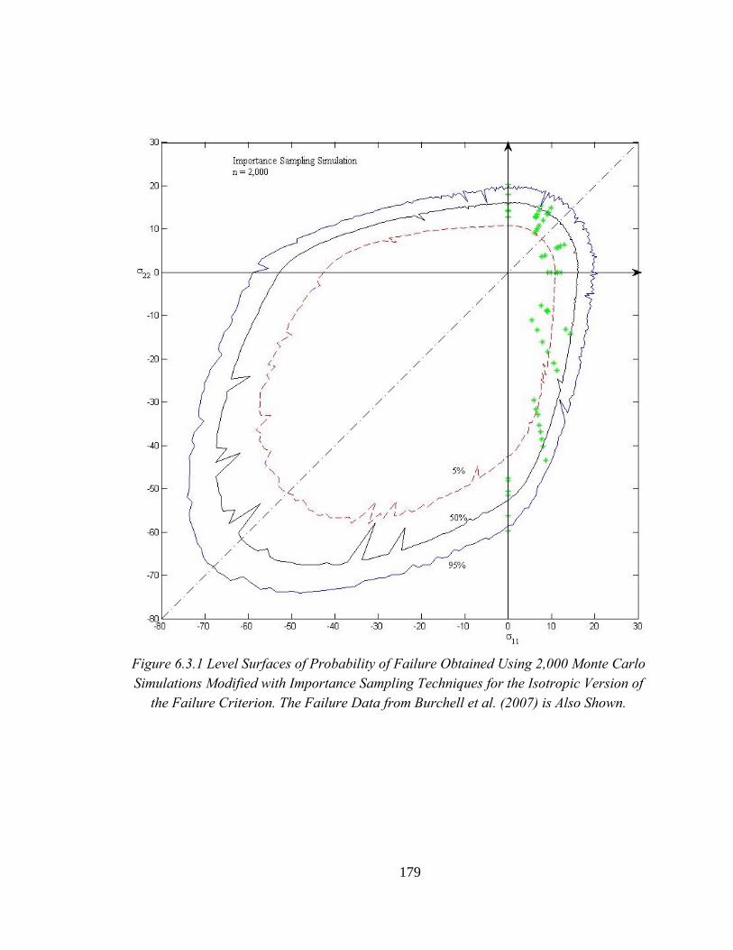
179
Figure 6.3.1 Level Surfaces of Probability of Failure Obtained Using 2,000 Monte Carlo Simulations Modified with Importance Sampling Techniques for the Isotropic Version of
the Failure Criterion. The Failure Data from Burchell et al. (2007) is Also Shown.

180
Figure 6.3.2 Level Surfaces of Probability of Failure Obtained Using 5,000 Monte Carlo Simulations Modified with Importance Sampling Techniques for the Isotropic Version of
the Failure Criterion. The Failure Data from Burchell et al. (2007) is Also Shown.
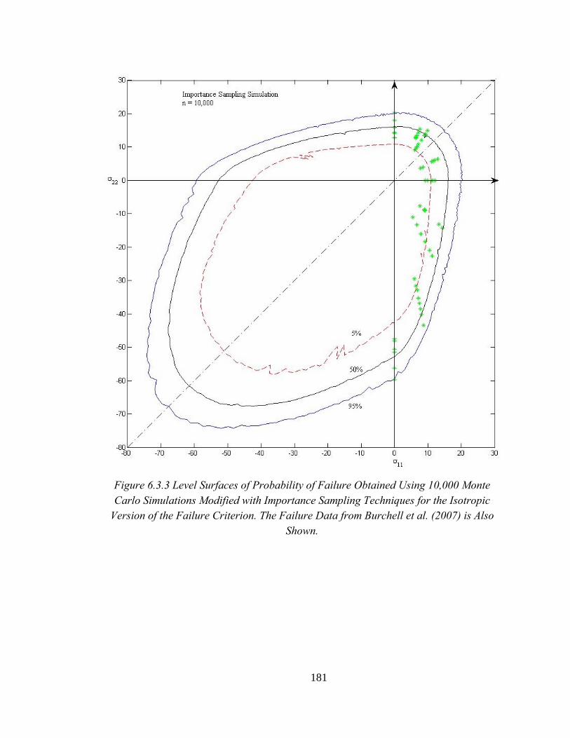
181
Figure 6.3.3 Level Surfaces of Probability of Failure Obtained Using 10,000 Monte Carlo Simulations Modified with Importance Sampling Techniques for the Isotropic
Version of the Failure Criterion. The Failure Data from Burchell et al. (2007) is Also Shown.
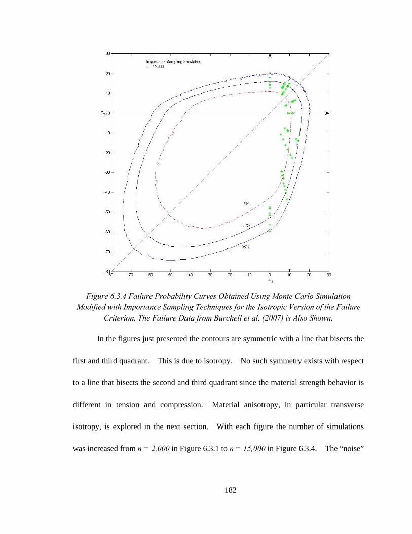
182
Figure 6.3.4 Failure Probability Curves Obtained Using Monte Carlo Simulation
Modified with Importance Sampling Techniques for the Isotropic Version of the Failure Criterion. The Failure Data from Burchell et al. (2007) is Also Shown.
In the figures just presented the contours are symmetric with a line that bisects the
first and third quadrant. This is due to isotropy. No such symmetry exists with respect
to a line that bisects the second and third quadrant since the material strength behavior is
different in tension and compression. Material anisotropy, in particular transverse
isotropy, is explored in the next section. With each figure the number of simulations
was increased from n = 2,000 in Figure 6.3.1 to n = 15,000 in Figure 6.3.4. The “noise”
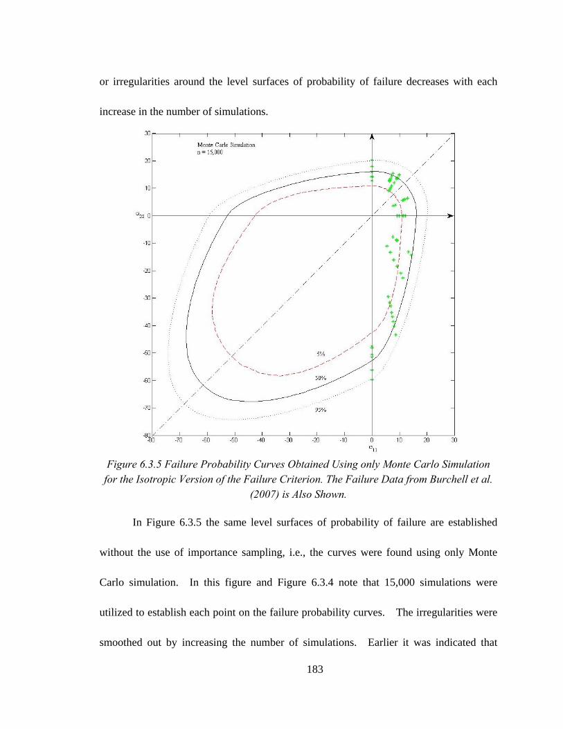
183
or irregularities around the level surfaces of probability of failure decreases with each
increase in the number of simulations.
Figure 6.3.5 Failure Probability Curves Obtained Using only Monte Carlo Simulation for the Isotropic Version of the Failure Criterion. The Failure Data from Burchell et al.
(2007) is Also Shown.
In Figure 6.3.5 the same level surfaces of probability of failure are established
without the use of importance sampling, i.e., the curves were found using only Monte
Carlo simulation. In this figure and Figure 6.3.4 note that 15,000 simulations were
utilized to establish each point on the failure probability curves. The irregularities were
smoothed out by increasing the number of simulations. Earlier it was indicated that
184
importance sampling is sensitive to the importance sampling function, i.e., Yk . It is
suspected that the irregularities in the probability of failure surfaces can also be smoothed
out with a more optimal choice in the standard deviation used for Yk . Time did not
permit conducting an optimization study for this parameter, and this effort is left for
others to conduct. Methods suggested in Xue et al. (2013) would be an appropriate
starting point. Once an optimization procedure has been established to compute a
standard deviation for the importance sampling function representing each random
strength variable it is anticipated that smooth curves can be obtained with fewer
simulations. It is clearly evident that increasing the number of simulations improves the
results obtained using importance sampling techniques. This is true for common Monte
Carlo simulation techniques as well – up to a point. At very low probability failures it
was clear (see Figure 6.2.3) that improving Monte Carlo simulation results was
impractical by simply increasing the number of simulations. This indicates that
importance sampling is the preferred method of computing equation (6.1.1) for typical
designs where the probability of failure is quite low for economic and/or safety reasons.
6.4 Anisotropic Limit State Functions – Importance Sampling
Next the concept of importance sampling is applied to the anisotropic form of the
limit state function. The tensile strength design variable in the preferred material
direction (YYT), the compressive strength design variable in the preferred material

185
direction (YYC), the equal biaxial compressive strength design variable in the plane of
isotropy (YBC), the tensile strength design variable in plane of isotropy (YTT), the
compressive strength design variable in plane of isotropy (YTC), as well as the equal
biaxial compressive strength design random variable with one stress component in the
plane of isotropy (YMBC) are characterized by the two-parameter Weibull distributions.
To begin the method the approximate location of the MPP must be determined.
The location of the MPP is determined through the realizations TTz , TCz , BCz , YTz ,
YCz and MBCz . By equation (6.2.1) all six are realizations of standard normal
variables. With these realizations serving as the components of a vector in the design
variable space, the MPP is located by this vector. The information regarding the MPP
establishes the means for the importance sampling density functions. Again, the
importance sampling density functions facilitate obtaining samples in the near vicinity of
the MPP during simulation. Once the means TTYk ,
TCYk , BCYk ,
YTYk , YCYk and
MBCYk are computed using equation (6.2.11) then the values TTYk ,
TCYk , BCYk ,
YTYk ,
YCYk and MBCYk are established using equation (6.2.12). These last six parameters are
the variances of the importance sampling density function. Use of equations (6.2.11)
and (6.2.12) requires the knowledge of the means from the parent Weibull strength
distributions, i.e., TTYf
, TCYf
, BCYf
, YTYf
, YCYf
and MBXCYf
as well as the standard
deviations of the parent Weibull strength distributions, i.e., TTYf
, TCYf
, BCYf
, YTYf
,
YCYf and
MBCYf .
186
Once the means and standard deviations are obtained for each importance
sampling density function the next step requires six separate and distinct random numbers
between zero and one. These will serve as values for TTYK in the expression
21
2
1
TT
TT
TT
Y
YTTY
yerfK
(6.4.1)
for TCYK in the expression
21
2
1
TC
TC
TC
Y
YTCY
yerfK
(6.4.2)
for BCYK in the expression
21
2
1
BC
BC
BC
Y
YBCY
yerfK
(6.4.3)
for YTYK in the expression
21
2
1
YT
YT
YT
Y
YYTY
yerfK
(6.4.5)
for YCYK in the expression
21
2
1
YC
YC
YC
Y
YYCY
yerfK
(6.4.6)
and for MBCYK in the expression
21
2
1
MBC
MBC
MBC
Y
YMBCY
yerfK
(6.4.7)
The only unknowns in these expressions are the realizations of the random strength
variables YTT, YTC, YBC, YYT, YYC and YMBC. These realizations are obtained by inverting
the last six expressions for these quantities.

187
Having realizations TTy , TCy , BCy , YTy , YCy and MBCy along with means
TTYk , TCYk ,
BCYk , YTYk ,
YCYk and MBXCYk as well as variances
TTYk , TCYk ,
BCYk , YTYk
, YCYk and
MBCYk then values of the sampling probability density functions
2
2
1exp
2
1
TTY
TTY
TTY
TT
k
kTT
k
TTY
yyk
(6.4.8)
2
2
1exp
2
1
TCY
TCY
TCY
TC
k
kTC
k
TCY
yyk
(6.4.9)
2
2
1exp
2
1
BCY
BCY
BCY
BC
k
kBC
k
BCY
yyk
(6.4.10)
2
2
1exp
2
1
YTY
YTY
YTY
YT
k
kYT
k
YTY
yyk
(6.4.11)
2
2
1exp
2
1
YCY
YCY
YCY
YC
k
kYC
k
YCY
yyk
(6.4.12)
as well as
2
2
1exp
2
1
MBCY
MBCY
MBCY
MBC
k
kMBC
k
MBCY
yyk
(6.4.13)
can be computed. The value of the joint probability sampling function for the jth
simulation is then ascertained using
jMBCYjYCYjYTYjBCYjTCYjTTY
MBCYCYTBCTCTTj
ykykykykykyk
YYYYYYk
MBCYCYTBCTCTT
,,,,, (6.4.14)
This joint probability sampling function is centered over the MPP

188
Realizations for the random strength variables YTT, YTC, YBC, YYT, YYC and YMBC
along with Weibull parameter (m, ) for each random strength variable are then used to
evaluate the probability of density function
TTTT
TT
m
TT
TT
m
TT
TT
TT
TTTTY
yymyf
exp
1
(6.4.15)
TCTC
TC
m
TC
TC
m
TC
TC
TC
TCTCY
yymyf
exp
1
(6.4.16)
BCBC
BC
m
BC
BC
m
BC
BC
BC
BCBCY
yymyf
exp
1
(6.4.17)
YTYT
TT
m
YT
YT
m
YT
YT
YT
YTYTY
yymyf
exp
1
(6.4.18)
YCYC
YC
m
YC
YC
m
YC
YC
YC
YCYCY
yymyf
exp
1
(6.4.19)
and
MBCMBC
MBC
m
MBC
MBC
m
MBC
MBC
MBC
MBCMBCY
yymyf
exp
1
(6.4.20)
respectively. A numerical value for the joint probability density
jMBCYjYCYjYTY
jBCYjTCYjTTY
MBCYCYTBCTCTTj
yfyfyf
yfyfyf
YYYYYYf
MBCYCYT
BCTCTT
,,,,,
(6.4.21)
is computed.
189
Finally, a value for the limit state function is computed using equations (5.2.1),
(5.2.13), (5.2.30) as well as (5.2.43) with the state of stress at the point in a component
being evaluated and the realizations of the random strength variables. This allows the
computation of the indicator function using equation (6.1.3). The quantities kj(yTT, yTC ,
yBC, yYT, yYC, yMBC ), fj(yTT, yTC , yBC, yYT, yYC, yMBC ) and I are inserted into equation
(6.2.13) and the summation in equation (6.2.14) is performed for a sufficient number of
iterations (i.e., large enough n) such that the method converges appropriately to Pf.
Figure 6.4.1 depicts the reliability surfaces for the anisotropic version of the
limit state function. Monte Carlo simulations with importance sampling were conducted
in order to generate the surfaces in this figure. For anisotropy the Weibull distribution
parameters for each random strength variable are listed in Table 6.4.1. Again three
reliability surfaces are depicted in the figure that correspond to probabilities of failure of
Pf = 5% , Pf = 50% , and Pf = 95%. The preferred direction of the material coincides
with the 11 axis. Thus there is a strengthening of the material along the 11 – axis
which is exhibited in the data from Burchell et al. (2007). The three curves bracket the
data from Burchell et al. (2007) along both the tensile and compressive 11 axes. This
reliability model captures this strengthening in compression as it did with the isotropic
model. The positions of the curve can be adjusted by information from the failure data
along both the 11 and 22 axes – tensile information as well as compression information.
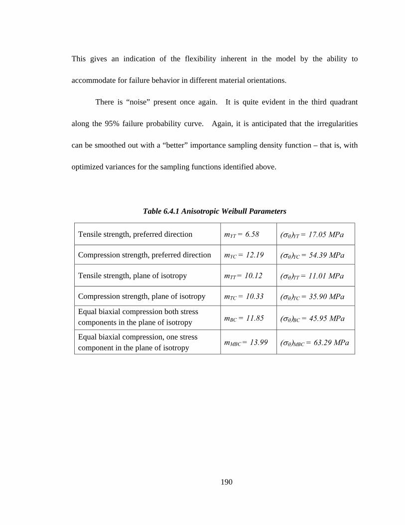
190
This gives an indication of the flexibility inherent in the model by the ability to
accommodate for failure behavior in different material orientations.
There is “noise” present once again. It is quite evident in the third quadrant
along the 95% failure probability curve. Again, it is anticipated that the irregularities
can be smoothed out with a “better” importance sampling density function – that is, with
optimized variances for the sampling functions identified above.
Table 6.4.1 Anisotropic Weibull Parameters
Tensile strength, preferred direction mYT = 6.58 YT = 17.05 MPa
Compression strength, preferred direction mYC = 12.19 YC = 54.39 MPa
Tensile strength, plane of isotropy mTT = 10.12 TT = 11.01 MPa
Compression strength, plane of isotropy mTC = 10.33 TC = 35.90 MPa
Equal biaxial compression both stress components in the plane of isotropy mBC = 11.85 BC = 45.95 MPa
Equal biaxial compression, one stress component in the plane of isotropy
mMBC = 13.99 MBC = 63.29 MPa

191
Figure 6.4.1 The Failure Data from Burchell et al. (2007) with Probability of Failure Curves Obtained Using Monte Carlo Simulation Modified with Importance Sampling
Techniques for the Anisotropic Version of the Failure Criterion.

192
CHAPTER VII
SUMMARY AND CONCLUSIONS
This dissertation presents a multiaxial reliability model that captures the complex
failure behavior of components fabricated from graphite. Of specific interest are
graphite components that are deployed throughout the core of nuclear reactors. The
failure behavior of graphite presents several unique challenges for the design engineer.
First, bulk strength is different under tensile stress states in comparison to compressive
stress states. In addition, depending on the how the material is produced, graphite can
exhibit isotropic or anisotropic failure behavior. The reliability models derived under
this effort can account for either and the isotropic reliability model discussed earlier is a
special case of the anisotropic model. At the present time anisotropic behavior is
limited to stochastic failure that can be characterized as transversely isotropic. Other
types of material symmetry, e.g., orthotropic failure behavior, can be accommodated
using the stress invariant/integrity basis techniques utilized herein.

193
7.1 Comparison With the ASME Simplified Assessment Method
As part of the summary a brief comparison of the reliability models developed
here is made with the stochastic methods advocated for in the ASME Boiler and Pressure
Vessel Code. The design, integrity and functionality of graphite core components found
in a nuclear reactor operating at elevated temperatures are controlled by a number of
subsections of the “ASME Boiler and Pressure Vessel Code Section III - Rules for
Construction of Nuclear Facility Components - Division 5 - High Temperature Reactors”
(2010). Hereafter this document is simply referred to as the ASME Code, or the code.
The ASME Code Article HHA 3200 entitled “Design by Analysis – Graphite Core
Components” delineates a number of engineering issues. This particular section
contains articles entitled “Requirements for Acceptability” (HHA 211), “Detailed
Requirements for Derivation of the Material Data Sheet – As-Manufactured Properties”
(HHA-II-3000), “Basis for Determining Stresses” (HHA 3213), “Stress Analysis” (HHA
3215), “Calculation of Probability of Failure” (HHA 3217), and “Stress Limits for
Graphite Core Component – Simplified Assessment” (HHA 3220). All have specific
relevance to this comparison made to work presented in this dissertation.
The acceptability of design under the ASME Code can be established by meeting
the requirements of a simplified assessment. The simplified assessment is conservative
and is outlined in HHA-3220 which points to the other sections of the code just
mentioned. This particular code article outlines the fundamental elements of a static
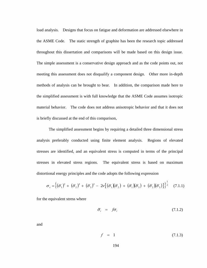
194
load analysis. Designs that focus on fatigue and deformation are addressed elsewhere in
the ASME Code. The static strength of graphite has been the research topic addressed
throughout this dissertation and comparisons will be made based on this design issue.
The simple assessment is a conservative design approach and as the code points out, not
meeting this assessment does not disqualify a component design. Other more in-depth
methods of analysis can be brought to bear. In addition, the comparison made here to
the simplified assessment is with full knowledge that the ASME Code assumes isotropic
material behavior. The code does not address anisotropic behavior and that it does not
is briefly discussed at the end of this comparison,
The simplified assessment begins by requiring a detailed three dimensional stress
analysis preferably conducted using finite element analysis. Regions of elevated
stresses are identified, and an equivalent stress is computed in terms of the principal
stresses in elevated stress regions. The equivalent stress is based on maximum
distortional energy principles and the code adopts the following expression
2
1
3231212
32
22
1 2 v (7.1.1)
for the equivalent stress where
ii f (7.1.2)
and
1f (7.1.3)

195
if the principal stress is tensile. If the principal stress is compressive then
tcR
f1
(7.1.4)
Here Rtc is the ratio of the mean compressive strength to the mean tensile strength. In
addition, is Poisson’s ratio and for graphite this material constant is taken equal to 0.15.
The expression for the equivalent stress can be incorporated into a limit state function
easily. That limit state function would be expressed as
T
g 1 (7.1.5)
where T represents the tensile strength of the material. The tensile strength parameter
is then treated as a random variable and reliability calculation proceed in a manner
identical to the methods outlined in Chapter 6.
The code requires information regarding the mean strength of the compressive
random variable in order to compute Rtc and subsequently the equivalent stress at any
point. In statistics the mean value of a random variable is considered a location
parameter for any density function whether the density function is a normal (Gaussian)
density function or not. However, the code does not require, nor does it utilize any
stochastic information relative to the scatter in compressive strength. The code
considers the stochastic properties of the tensile random strength variable by using the
Weibull characteristic strength (a location parameter) and the Weibull modulus (a

196
measure of scatter or variance). The ASME Code embraces the tensile strength as a
random variable in a comprehensive manner but does not do the same with the
compressive strength random variable. The ASME Code effectively ignores stochastic
information relative to the compressive strength of the material by discarding the scatter
quantified by the associated Weibull modulus. This is done with the thought that this
simplifies design procedures.
The ASME limit state function in equation (7.1.5) is an isotropic failure criterion.
It has been noted throughout that data from Burchell et al. (2007) represents anisotropic
failure behavior. As will be seen momentarily, the data from Burchell et al. (2007) is
convenient in facilitating a comparison between the reliability models derived here and
the ASME based reliability models. As a work around the tensile and compressive
mean strengths from the data found in Burchell et al. (2007) in the preferred direction can
be used to compute a value for Rtc.. With a value of the ratio of mean strengths and the
Weibull parameters from tensile strength stress data one can map the probability of
failure curve depicted in Figure 7.1.1 using equation (7.1.5). In this figure the 50%
probability of failure curve is projected into the 11 –22 stress space. The curve bisects
the data from Burchell et al. (2007) along the 11–axis as it should. This stress axis
coincides with the preferred (strong) direction of the material. The 50% probability of
failure curve should be in close proximity with the mean values of the tensile and
compressive strength data, and from the figure it is evident this happens.

197
Figure 7.1.1 ASME Maximum Distortional Energy Probability of Failure Curve (50%)
with the Failure Data from Burchell et al. (2007).
As a comparison, the isotropic reliability model derived here is also projected into
a 11 –22 stress space in Figure 7.1.2 along with the maximum distortional energy
reliability model just presented. Both reliability curves are characterized using the data
from Burchell et al. (2007) in the strong direction of the material. The 50% probability
of failure curve generated by simulation was presented in the previous chapter. It is
evident in this figure that the ASME maximum distortional energy reliability curve is
more conservative than the isotropic reliability curve. This is starkly apparent in the

198
biaxial compression regions of the stress space. The isotropic reliability model is
controlled by the biaxial strength parameter, BC, along this stress path. Adjustment in
the isotropic reliability model can be made along this stress path through this parameter
indicating a degree of flexibility has been built into the model. No such flexibility exists
in the ASME models along this stress path. Since failure data is unavailable for an
equal biaxial stress load path because of the difficulty of attaining this state of stress in a
test specimen, future efforts should include an optimization algorithm to determine the
Weibull parameters for the biaxial compression strength random variable, BC.
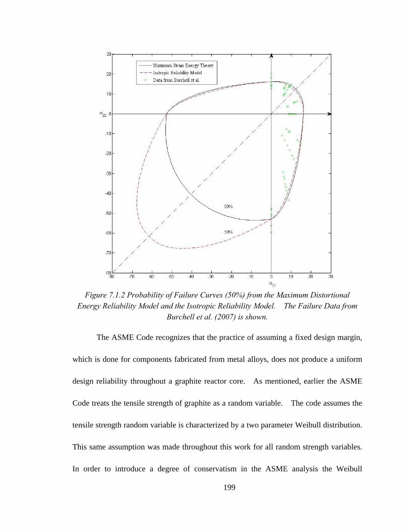
199
Figure 7.1.2 Probability of Failure Curves (50%) from the Maximum Distortional
Energy Reliability Model and the Isotropic Reliability Model. The Failure Data from Burchell et al. (2007) is shown.
The ASME Code recognizes that the practice of assuming a fixed design margin,
which is done for components fabricated from metal alloys, does not produce a uniform
design reliability throughout a graphite reactor core. As mentioned, earlier the ASME
Code treats the tensile strength of graphite as a random variable. The code assumes the
tensile strength random variable is characterized by a two parameter Weibull distribution.
This same assumption was made throughout this work for all random strength variables.
In order to introduce a degree of conservatism in the ASME analysis the Weibull
200
parameters extracted from the tensile strength data are “knocked down.” The code
calls for the use of Weibull parameters that correspond to the lower limit of the 95%
confidence bound on the estimated parameters. At the time this dissertation was written
the expression in the ASME code for the “knocked down” value of the Weibull
characteristic strength at the lower bound of 95% confidence bound was incorrect. The
correct relationship for the 95% lower bound on the Weibull characteristic strength is
used here. The effects of the “knocked down” Weibull parameters called for in the
ASME code are in evidence in Figure 7.1.3. As a result of using the “knocked down”
Weibull parameters the ASME maximum distortional energy probability of failure curve
shrinks isotropically The stress states that correspond to the 50% failure probability
using the “knocked down” Weibull parameters are smaller in magnitude relative to those
in the previous figure. This imposes an unknown degree of conservatism on the design
of graphite reactor core components. The 95% lower bound on Weibull parameter
estimates does not correspond to a 95% lower bound on component reliability.

201
Figure 7.1.3 Probability of Failure Curves (50%) Using the ASME Method with the Reduced Weibull Parameters and the Isotropic Reliability Model. The Failure Data
from Burchell et al. (2007) is Included.
In order to paint a comprehensive picture of the maximum distortional energy
reliability model a nested set of reliability curves are presented in the next figure. Keep
in mind that data from Burchell et al. (2007) along the tensile and compressive 11-axis is
used as proscribed in the ASME code, i.e., “knocked down” Weibull parameters are used
in Figure 7.1.4. The spacing between the curves is controlled by the Weibull modulus
obtained from the tensile data. This aspect of the ASME approach should be
interrogated in future efforts.

202
Figure 7.1.4 Nested Reliability Surfaces Using ASME Code Methods to Determine Reliability. The Failure Data from Burchell et al. (2007) is Depicted.
These curves correspond to failure probabilities of 5%, 50% and 95% and they
should be compared to the reliability curves found in Figure 6.3.5. Note that the 95%
probability of failure curve in Figure 7.1.4 is beyond the last compressive failure data
point along the 11-axis. This seems to infer a bit of non-conservatism for compressive
loads. The 95% probability of failure curve for the isotropic reliability model developed
here is in close proximity to the largest compressive failure stress in Figure 6.3.5. This
would indicate that the probability of failure curve in Figure 6.3.5 for the isotropic
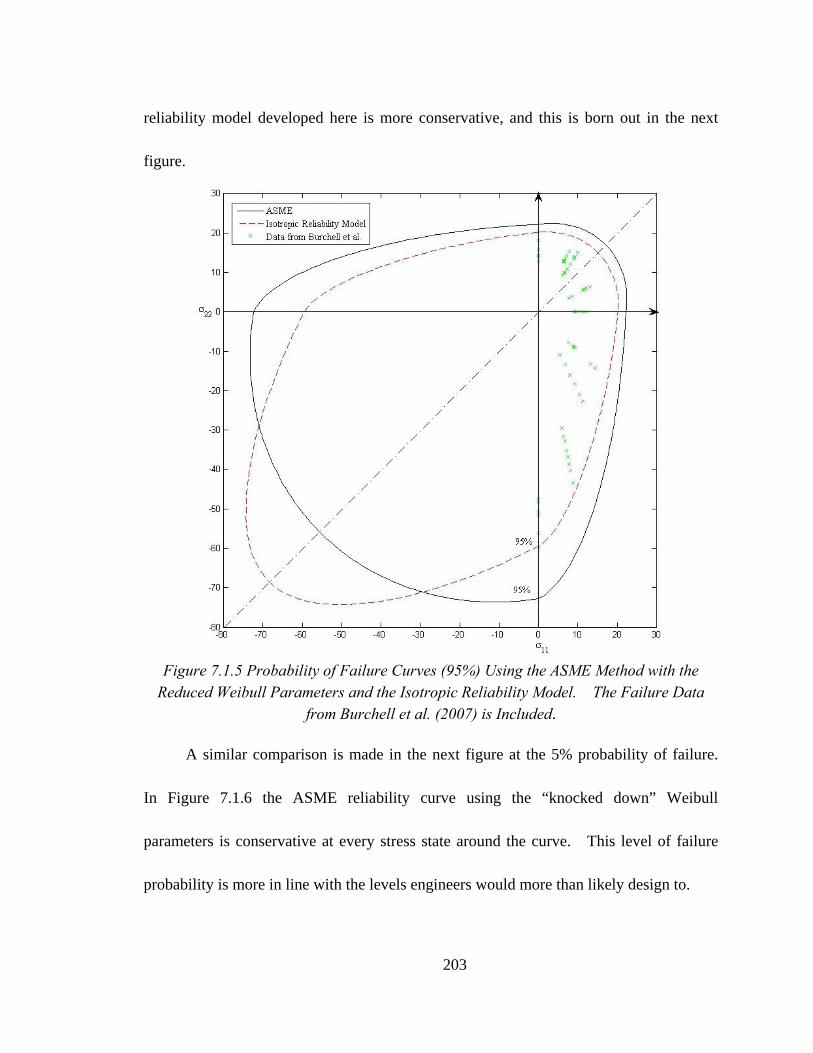
203
reliability model developed here is more conservative, and this is born out in the next
figure.
Figure 7.1.5 Probability of Failure Curves (95%) Using the ASME Method with the
Reduced Weibull Parameters and the Isotropic Reliability Model. The Failure Data from Burchell et al. (2007) is Included.
A similar comparison is made in the next figure at the 5% probability of failure.
In Figure 7.1.6 the ASME reliability curve using the “knocked down” Weibull
parameters is conservative at every stress state around the curve. This level of failure
probability is more in line with the levels engineers would more than likely design to.

204
Figure 7.1.6 Probability of Failure Curves (5%) Using the ASME Method with the
Reduced Weibull Parameters and the Isotropic Reliability Model. The Failure Data from Burchell et al. (2007) is Included.
Finally in Figures 7.1.5 and 7.1.6 the ASME reliability models are compared to
the predictions from the anisotropic reliability model derived in this work. Again, all
models are characterized using the data from Burchell et al. (2007). The first
comparison of the anisotropic curve developed here is made with the ASME maximum
distortional energy curve. Both curves appear in Figure 7.1.1 and both curves
correspond to a failure probability of 50%
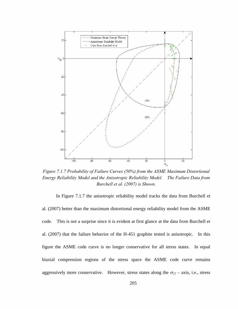
205
Figure 7.1.7 Probability of Failure Curves (50%) from the ASME Maximum Distortional Energy Reliability Model and the Anisotropic Reliability Model. The Failure Data from
Burchell et al. (2007) is Shown.
In Figure 7.1.7 the anisotropic reliability model tracks the data from Burchell et
al. (2007) better than the maximum distortional energy reliability model from the ASME
code. This is not a surprise since it is evident at first glance at the data from Burchell et
al. (2007) that the failure behavior of the H-451 graphite tested is anisotropic. In this
figure the ASME code curve is no longer conservative for all stress states. In equal
biaxial compression regions of the stress space the ASME code curve remains
aggressively more conservative. However, stress states along the 22 – axis, i.e., stress

206
states that corresponds to tensile and compressive strengths in the plane of isotropy, the
ASME curve is no longer conservative. This reflects the fact that the anisotropic model
allows for more information regarding the strengths of the material as well as by the fact
that the ASME model is characterized with failure data oriented in the strong direction of
the material, i.e., along the 11-axis. The fact that the ASME model does not track the
s22 failure stresses well should not surprise. There is no provision in the ASME Code
for anisotropic failure behavior. A conservative approach would be the utilization of the
weak axis failure data, i.e., failure data in the plane of isotropy. At the present time that
is not called for specifically in the ASME Code.

207
Figure 7.1.8 Probability of Failure Curves (50%) Using the ASME Method with the
Reduced Weibull Parameters and the Anisotropic Reliability Model. The Failure Data from Burchell et al. (2007) is Included.
When the anisotropic model is compared to the ASME model with “knocked
down” Weibull parameters the conservatism of the anisotropic model in the plane of
isotropy is greatly diminished. When the comparison is made at the 5% probability of
failure level the ASME model with the “knocked down” Weibull parameters is more
conservative at any stress point on the reliability curve. This can be seen in Figure
7.1.9.
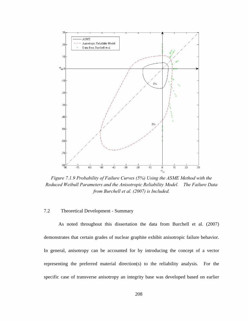
208
Figure 7.1.9 Probability of Failure Curves (5%) Using the ASME Method with the
Reduced Weibull Parameters and the Anisotropic Reliability Model. The Failure Data from Burchell et al. (2007) is Included.
7.2 Theoretical Development - Summary
As noted throughout this dissertation the data from Burchell et al. (2007)
demonstrates that certain grades of nuclear graphite exhibit anisotropic failure behavior.
In general, anisotropy can be accounted for by introducing the concept of a vector
representing the preferred material direction(s) to the reliability analysis. For the
specific case of transverse anisotropy an integrity base was developed based on earlier
209
work of Green and Mkrtichian (1977). They developed their integrity basis in order to
derive an isotropic constitutive model for non-linear elastic behavior. The non-linear
stress-strain model accounted for different elastic deformation behavior in tension and
compression by introducing a direction vector to the integrity basis that tracked the
direction of the maximum principal stress. Their integrity basis was modified to
account for a preferred direction in a material – that is, to account for material anisotropy
exhibited in the failure behavior of nuclear graphite. This required a second vector in
order to track material anisotropy. The second vector coincides with the preferred
direction of the material, i.e., the “strong” direction of the material. Thus the integrity
basis assembled here accounts for two directions – on associated with the stress state of
the material and a second associated with material symmetry.
This integrity basis was constructed following the framework advocated for in
Rivlin and Smith (1969) as well as Spencer (1971, 1984). This work focused on
isotropic failure behavior first. A linear combination of the invariants identified by
Green and Mkrtichian (1977) were used to formulate for four separate isotropic failure
functions for each region of the principal stress space defined by the relative magnitudes
of the principal stresses. The linear combination of invariants serves as the limit state
function for materials with different failure behavior in tension and compression.
Constants associated with the linear combination were identified for each stress region in
terms of simple mechanical test data. This identified the fundamental strength
210
parameters that were later treated as random variables in transitioning from deterministic
models of limit state functions to reliability models. When the isotropic integrity basis
adopted from the work of Green and Mkrtichian (1977) was extended to account for
material anisotropy additional material strength parameters were identified. These
additional strength parameters that were similarly treated as random strength variables for
the anisotropic reliability model. Developing an isotropic failure criterion for graphite,
transforming that failure criterion into a reliability model, and extending both to
transverse isotropy represent the primary contribution to the body of knowledge made
during this research project.
The transformation from a deterministic failure criterion to a reliability model was
enabled numerically through the use of Monte Carlo simulations augmented with
importance sampling. This makes the reliability model amenable for use in engineering
design. States of stress in a graphite core component can be analyzed using finite
element analysis and subsequently reliability evaluations can be conducted at each
integration point of an element within the finite element mesh. This approach is
advocated for at select points in a reactor component in the ASME Code. This is also
the analytical structure utilized in the NASA CARES software algorithms (Gyekenyesi,
1986), but in a more comprehensive fashion.
211
7.3 Conclusions and Future Efforts
Research projects can raise more questions then are answered. This project took
on that quality near the end. When the isotropic model was extended to capture
transverse anisotropy failure behavior the model tracked failure behavior seen in the data
from Burchell et al. (2007). The transversely isotropic model was characterized using
data from Burchell et al. (2007) so the model should mimic the data used in
characterizing the model, or the model is seriously flawed. Typically with analytical
models one should characterize the model with data from one type of test specimen.
The model should then be interrogated by asking the model to predict the behavior from a
test specimen with a completely different specimen geometry and load configuration.
The anisotropic reliability model can and should be characterized by the data from
Burchell et al. (2007), which was done here. The model should then be used to predict
failure probabilities say for an L-shaped bracket that is representative of reactor core
components. The predictions from the model for the second test specimen geometry
should be compared to the failure data from the L-shaped bracket geometry and
conclusions regarding model performance can be drawn. This assumes the L-shaped
brackets, or other type of test specimen with a complex stress distribution, is fabricated
from the same material used to characterize the model.
This approach has been advocated in Department of Energy (DoE) research
programs and internationally collaborative industry program with a focus on nuclear
212
grade graphite. To date this strategy has not been completely implemented for a
particular material. Even if testing had taken place for the two types of test specimen
the finite element analysis required to make this comparison is beyond the work scope
here. This is another task for others to assess in the future.
Reliability calculations made using the models developed here required numerical
methods for evaluation. The simplest approach, i.e., Monte Carlo simulation, was
shown to be ineffective at low probabilities of failure. Too much error is present even at
extremely large numbers of simulations. Yet low probabilities of failure is where an
engineer wishes to operate a system of components. Importance sampling mitigated
issues at low probability of failures, but the sense here is that the sampling density
functions can and should be optimized somehow. Others following up on this research
effort should look seriously into this issue.
With regards to failure analysis for material with material symmetries other than
transversely isotropic, the extension of a phenomenological failure criterion was made
here for transversely isotropic failure behavior. In the future other material symmetries,
e.g., materials with orthotropic failure behavior, can be accommodated as well. Duffy
and Manderscheid (1990b) as well as others have suggested an appropriate integrity basis
for the orthotropic material symmetry. These should be studied in conjunction with the
integrity basis outlined in the work of Green and Mkrtichian (1977).
213
Finally, the ASME design code is in need of a comprehensive software algorithm
to aid design engineers in qualifying components. This algorithm must enable the
design engineer to calculate the reliability of graphite core components as a system where
the stress state at every point in the component contributes to a reduction of component
reliability, not just a select number of locations of high stress. This admits the
possibility of failure occurring at any point in a reactor component. Unfortunately, the
size effect of graphite is somewhat enigmatic. As Nemeth and Bratton (2012) as well as
others point out certain size effects in graphite materials is hard to characterize. With
regard to system reliability materials can act as a weakest link system where failure at a
point is catastrophic. Other materials can act as a series system where failure must take
place at every point in the system for failure to occur. The suspicion here is that
graphite acts like an “r out of n” system where failure of the system occurs after a finite
number of failures have occurred throughout the component. This concept should be
pursued in future efforts.

214
REFERENCES
ASME Boiler and Pressure Vessel Code, ASME, Section III, Division 5, 2010. Balzer, M.A., “Mechanical Behavior of Metals under Triaxial Stress: Apparatus and Experiments,” Ph.D. Dissertation, University of Illinois at Urbana-Champaign, 1998. Batdorf, S.B. and Crose, J.G., “A Statistical Theory for the Fracture of Brittle Structure Subjected to Nonuniform Polyaxial Stress,” ASME Journal of Applied Mechanics, Vol. 41, No. 2, pp. 459-464, 1974. Boehler, J.P. and Sawczuk, A., “On Yielding of Oriented Solids,” Acta Mechanica, Vol. 27, pp. 185-204, 1977. Boehler, J.P., Kirillov, A.A. and Onat, E.T., “On the Polynomial Invariants of the Elasticity Tensor,” Journal of Elasticity, Vol 34, pp. 97-110, 1994. Boehler, J.P., “Yielding and Failure of Transversely Isotropic Solids, Applications of Tensor Functions in Solid Mechanics,” CISM Courses and Lectures No 292, Springer-Verlag, Berlin, pp. 3-140, 1987. Boresi, A.P. and Schmidt, R.J., Advanced Mechanics of Materials, 6th Edition, John Wiley and Sons, Inc., pp.117-129, 2003. Bridgman, P.W., “The Effect of Pressure on the Tensile Properties of Several Metals and Other Materials,” Journal of Applied Physics, Vol. 24, No. 5, pp.560-570, 1953. Burchell, T., Yahr, T. and Battiste, R., “Modeling the Multiaxial Strength of H-451 Nuclear Grade Graphite,” Carbon, Vol. 45, No. 13, pp. 2570-2583, 2007. Burchell, T.D. (editor), Carbon Materials for Advanced Technologies, Elsevier, 1999. Cazacu, O., Cristescu, N.D., Shao, J.F. and Henry, J.P., “A New Anisotropic Failure Criterion for Transversely Isotropic Solids,” Mechanics Cohesive-Frictional Material, Vol. 3, pp. 89-103, 1998. Cazacu, O. and Cristescu, N.D., “A Paraboloid Failure Surface For Transversely Isotropic Materials,” Mechanics of Materials, Vol. 31, No. 6, pp. 381-393, 1999.

215
Cooper, N.R., Margetson, J., and Humble, S., “Probability of Failure Calculations And Confidence Brand Estimates For An Annular Brittle Disc Fracture Under Centrifugal Loading,” Journal of Strain Analysis for Engineering Design, Vol. 21, No. 3, 121-126, 1986. Cooper, N.R., “Probabilistic Failure Prediction of Rocket Motor Components,” Ph.D. Dissertation, Royal Military College of Science, 1988. Coulomb, C.A., “Essai sur une Application des Regles des Maximis et Minimis a Quelquels Problemesde Statique Relatifs, a la Architecture,” Memoires de Mathematique et de Physique, presentes a l’Academie Royales Des Sciences, Vol. 7, pp. 343–387, 1776. Drucker, D.C. and Prager, W., “Soil Mechanics and Plastic Analysis For Limit Design,” Quarterly of Applied Mathematics, Vol. 10, No. 2, pp. 157–165, 1952. Duffy, S.F., “A Viscoplastic Constitutive Theory for Transversely Isotropic Metal Alloys,” Ph.D. Dissertation, University of Akron, 1987. Duffy, S.F. and Gyekenyesi, J.P., “Time Dependent Reliability Model Incorporating Continuum Damage Mechanics for High-Temperature Ceramics,” NASA Technical Memorandum 102046, 1989. Duffy, S.F. and Arnold, S.M., “Noninteractive Macroscopic Reliability Model for Whisker-Reinforced Ceramic Composites,” Journal of Composite Materials, Vol. 24, No. 3, pp.235-344, 1990a. Duffy, S.F. and Manderscheid, J.M., "Noninteractive Macroscopic Reliability Model for Ceramic Matrix Composites with Orthotropic Material Symmetry," Journal of Engineering for Gas Turbines and Power, Vol. 112, No. 4, pp. 507 511, 1990b. Duffy, S.F., Chulya, A. and Gyekenyesi, J.P., “Structural Design Methodologies for Ceramic-Based Material Systems,” NASA Technical Memorandum 103097, 1991. Duffy, S.F., Wetherhold, R.C. and Jain, L.K., "Extension of a Noninteractive Reliability Model for Ceramic Matrix Composites," Journal of Engineering for Gas Turbines and Power, Vol. 115, No. 1, pp. 205 207, 1993.
216
Duffy, S.F., and Palko, J.L., “Analysis of Whisker Toughened CMC Structural Components Using an Interactive Reliability Model,” AIAA Journal, Vol. 32, No. 5, pp. 1043-1048, 1994. Duffy, S.F., Baker, E.H., and James, C., "Standard Practice for Reporting Uniaxial Strength Data And Estimating Weibull Distribution Parameters For Graphite," ASTM Standard D 7846, 2013. Green, A.E. and Mkrtichian, J.Z., “Elastic Solids with Different Moduli in Tension and Compression,” Journal of Elasticity, Vol. 7, No. 4, pp. 369-386, 1977. Griffiths, A.A., “The Theory Of Rupture And Flow In Solids,” Philosophical Transactions of the Royal Society A: Mathematical, Physical and Engineering Sciences, Vol. 221, pp. 163-198, 1921. Gyekenyesi, J.P., “SCARE - A Post-Processor Program to MSC/NASTRAN for the Reliability Analysis of Ceramic Components,” ASME Journal of Engineering for Gas Turbines and Power, Vol. 108, No. 3, 540-546, 1986. Harbitz, A., “An Efficient Sampling Method for Probability of Failure Calculations,” Structural Safety, Vol. 3, pp. 108-115, 1986. Haldar, A. and Mahadevan, S., Reliability Assessment Using Stochastic Finite Element Analysis, John Wiley & Sons, 2000. Hu, J., “Modeling Size Effects and Numerical Methods in Structural Reliability Analysis,” Masters Thesis, Cleveland State University, 1994. Kaufman, M. and Ferrante, J., “Statistical Model for Mechanical Failure,” NASA Technical Memorandum 107112, 1996 Lamon, J., “Reliability Analysis of Ceramics Using the CERAM Computer Program,” ASME Paper No. 90-GT-98, IGTI, 1990. Li, Q.M., “Strain energy Density Failure Criterion,” International Journal of Solids and Structures, Vol. 38, No. 38, pp. 6997–7013, 2001. Melchers, R.E., “Importance Sampling in Structural Systems,“ Structural Safety, Vol. 6, pp. 3-10, 1989

217
Nova, R., and Zaninetti, A., “An Investigation Into the Tensile Behavior of a Schistose Rock,” International Journal of Rock Mechanics, Mining Sciences and Geomechanics, Vol. 27, No. 4, pp. 231-242, 1990. Palko, J.L., “An Interactive Reliability Model for Whisker- Toughened Ceramics,” Masters Thesis, Cleveland State University, June 1992. Paul, B., “Generalized Pyramidal Fracture and Yield Criteria,” International Journal of Solids and Structure, Vol. 4, pp.175-196, 1968. Romanoski, G.R. and Burchell, T.D., “Fracture in Graphite,” in Carbon Materials for Advanced Technologies, Burchell, T.D. (editor), Elsevier, pp. 485-534, 1999. Rivlin, R.S. and Smith, G.F., “Orthogonal Integrity Basis for N Symmetric Matrices,” in Contributions to Mechanics, ed. D. Abir, Pergamon Press, Oxford, pp. 121-141, 1969. Saito, S., “Role of Nuclear Energy to a Future Society of Shortage of Energy Resources and Global Warming,” Journal of Nuclear Materials, Vol. 398, pp. 1-9, 2010. Schleicher, F., “Der Spannungszustand an der Fließgrenze (Plastizitätsbedingung),” Zeitschrift für Angewandte Mathematik und Mechanik, Vol. 6, pp. 199- 216, 1926. Spencer, A.J.M., “Theory of Invariants,” in Continuum Physics, 1, ed. A.C. Eringen, Academic Press, London, pp. 259-353, 1971. Spencer, A.J.M., “Continuum Theory of the Mechanics of Fibre-Reinforced Composites,” Spring-Verlag, pp.1-32, 1984. Sun, C.T., and S.E. Yamada. "Strength Distribution of a Unidirectional Fiber Composite," Journal of Composite Materials, Vol. 12.2, pp. 169-176, 1978. Tabeddor, F., “A Survey of Constitutive Educations of Bimodulus Elastic Materials,” in Mechanics of Bimodulus Materials, ed: C.W. Bert, Proceedings of the American Society of Mechanical Engineering Winter Annual meeting, AMD33, 2–5, 1979. Tresca, H., “Mémoire sur L'écoulement des Corps Solides Soumis à de Fortes Pressions,” Comptes Rendus, Academie de Science, Vol. 59, p. 754, 1864.
218
Tsai, S.W. and Wu, E.M., “A General Theory of Strength of Anisotropic Materials,” Journal of Composite Materials, Vol. 5, pp. 58-80, 1971. Theocaris, P.S., “The Elliptic Paraboloid Failure Criterion for Cellular Solids and Brittle Foams,” Acta Mechanica, Vol. 89, pp. 93-121, 1991. US DOE Nuclear Energy Research Advisory Committee and the Generation IV International Forum, “A Technology Roadmap for Generation IV Nuclear Energy Systems,” GIF-002-00, December 2002. Vijayakumar, K. and Ashoka, J.G., “A Bilinear Constitutive Model for Isotropic Bimodulus Materials,” ASME Journal of Engineering Materials and Technology, Vol. 112, pp. 372-379, 1990. Vijayakumar, K., and Rao, K.P., “Stress-Strain Relations for Composites with Different Stiffness in Tension and Compression,” Computational Mechanics, Vol. 2, pp. 167-175, 1987. von Mises, R., “Mechanik der Festen Korper im Plastisch Deformablen Zustand,” Göttinger Nachrichten, pp. 582–592, 1913. Weibull, W., “A Statistical Distribution Function of Wide Applicability,” Journal of Applied Mechanics, Vol. 18, No. 3, pp. 293-297, 1951. Weibull, W., Ingeniors Vetenshaps Akadamein, Handlingar, 151 (1939) Wetherhold, R.C., “Statistics of Fracture of Composite Materials Under Multiaxial Loading,” PhD Dissertation, University of Delaware, 1983. Wetherhold, R.C. and Ucci, A.M., “Probability Techniques for Reliability Analyses of Composite Materials,” NASA CR-195294, National Aeronautics and Space Administration, National Technical Information Service, 1994. Willam, K.J. and Warnke, E.P., “Constitutive Models for the Triaxial Behavior of Concrete,” in: Proceedings of the International Association for Bridge and Structural Engineer Seminar on Structures Subjected to Triaxial Stresses (Bergamo, Italy), Vol. 19, pp. 1-31, 1974.

219
Xue, G.F., Dai, H.Z., and Zhang, H., “An Adaptive Importance Sampling Scheme for Efficient Reliability Analysis,” in Safety, Reliability, Risk and Life-Cycle Performance of Structure & Infrastructures – Deodatis, Ellingwood & Frangopo (Eds), Taylor & Francis Group, London, pp. 707- 713, 2013.