a primer for unit root testing (palgrave texts in econometrics)
TRANSCRIPT

A Primer for Unit Root Testing
Other books by Kerry Patterson
Patterson, K. D. An Introduction to Applied Econometrics: A Time Series Approach
Mills. T. C., and K. D. Patterson. (eds) Palgrave Handbook of Econometrics, Volume 1, Econometric Theory
Mills. T. C., and K. D. Patterson. (eds) Palgrave Handbook of Econometrics, Volume 2, Applied Econometrics
PalgraveTexts in Econometrics
General Editor: Kerry Patterson
Titles include:
Simon P. Burke and John HunterMODELLING NON-STATIONARY TIME SERIES
Michael P. ClementsEVALUATING ECONOMETRIC FORECASTS OF ECONOMIC AND FINANCIAL VARIABLES
Lesley GodfreyBOOTSTRAP TESTS FOR REGRESSION MODELS
Terence C. MillsMODELLING TRENDS AND CYCLES IN ECONOMIC TIME SERIES
Kerry PattersonA PRIMER FOR UNIT ROOT TESTING
Palgrave Texts in Econometrics
Series Standing Order ISBN 978–1–4039–0172–9 (hardback) 978–1–4039–0173–6 (paperback) (outside North America only)
You can receive future titles in this series as they are published by placing a standing order. Please contact your bookseller or, in case of difficulty, write to us at the address below with your name and address, the title of the series and the ISBN quoted above.
Customer Services Department, Macmillan Distribution Ltd, Houndmills, Basingstoke, Hampshire RG21 6XS, England

A Primer for Unit Root Testing
Kerry Patterson

© Kerry Patterson 2010
All rights reserved. No reproduction, copy or transmission of this publication may be made without written permission.
No portion of this publication may be reproduced, copied or transmitted save with written permission or in accordance with the provisions of the Copyright, Designs and Patents Act 1988, or under the terms of any licence permitting limited copying issued by the Copyright Licensing Agency, Saffron House, 6-10 Kirby Street, London EC1N 8TS.
Any person who does any unauthorized act in relation to this publication may be liable to criminal prosecution and civil claims for damages.
The author has asserted his right to be identified as the author of this work in accordance with the Copyright, Designs and Patents Act 1988.
First published 2010 byPALGRAVE MACMILLAN
Palgrave Macmillan in the UK is an imprint of Macmillan Publishers Limited,registered in England, company number 785998, of Houndmills, Basingstoke, Hampshire RG21 6XS.
Palgrave Macmillan in the US is a division of St Martin’s Press LLC, 175 Fifth Avenue, New York, NY 10010.
Palgrave Macmillan is the global academic imprint of the above companies and has companies and representatives throughout the world.
Palgrave® and Macmillan® are registered trademarks in the United States,the United Kingdom, Europe and other countries.
ISBN: 978–1–403–90204–7 hardbackISBN: 978–1–403–90205–4 paperback
This book is printed on paper suitable for recycling and made from fully managed and sustained forest sources. Logging, pulping and manufacturing processes are expected to conform to the environmental regulations of the country of origin.
A catalogue record for this book is available from the British Library.
A catalog record for this book is available from the Library of Congress.
10 9 8 7 6 5 4 3 2 119 18 17 16 15 14 13 12 11 10
Printed and bound in Great Britain byCPI Antony Rowe, Chippenham and Eastbourne

To Kaylem, Abdullah, Isaac Ana and Hejr

This page intentionally left blank
vii
Contents
List of Tables xvii
List of Figures xviii
Symbols and Abbreviations xx
Preface xxii
1 An Introduction to Probability and Random Variables 1
2 Time Series Concepts 45
3 Dependence and Related Concepts 85
4 Concepts of Convergence 105
5 An Introduction to Random Walks 129
6 Brownian Motion: Basic Concepts 160
7 Brownian Motion: Differentiation and Integration 181
8 Some Examples of Unit Root Tests 205
Glossary 258
References 262
Author Index 271
Subject Index 274

This page intentionally left blank
ix
Detailed Contents
List of Tables xvii
List of Figures xviii
Symbols and Abbreviations xx
Preface xxii
1 An Introduction to Probability and Random Variables 1 Introduction 1 1.1 Random variables 2 1.2 The probability space: Sample space, field, probability
measure (Ω, F, P) 3 1.2.1 Preliminary notation 3 1.2.2 The sample space Ω 4 1.2.3 Field (algebra, event space), F: Introduction 6 1.2.3.i Ω is a countable finite sample space 7 1.2.3.ii Ω is a countably infinite sample space;
–field or –algebra 8 1.2.3.iii Ω is an uncountably infinite sample space 9 1.2.3.iii.a Borel sets; Borel –field of 10 1.2.3.iii.b Derived probability measure
and Borel measurable function 11 1.2.4 The distribution function and the density
function, cdf and pdf 11 1.2.4.i The distribution function 11 1.2.4.ii The density function 12 Example 1.1: Uniform distribution 13 Example 1.2: Normal distribution 14 1.3 Random vector case 15 Example 1.3: Extension of the uniform
distribution to two variables 16 1.4 Stochastic process 17 1.5 Expectation, variance, covariance and correlation 19 1.5.1 Expectation and variance of a random variable 20 1.5.1.i Discrete random variables 20 1.5.1.ii Continuous random variables 21

x Contents
1.5.2 Covariance and correlation between variables 21 1.5.2.i Discrete random variables 22 1.5.2.ii Continuous random variables 22 Example 1.4: Bernoulli trials 22 1.6 Functions of random variables 23 1.6.1 Linear functions 23 Example 1.5: Variance of the sum of two
random variables 25 1.6.2 Nonlinear functions 25 1.7 Conditioning, independence and dependence 27 1.7.1 Discrete random variables 27 Example 1.6: The coin-tossing
experiment with n = 2 29 Example 1.7: A partial sum process 31 1.7.2 Continuous random variables 31 1.7.2.i Conditioning on an event A ≠ a 32 Example 1.8: The uniform joint
distribution 33 1.7.2.ii Conditioning on a singleton 34 1.7.3 Independence in the case of multivariate
normality 36 1.8 Some useful results on conditional expectations:
Law of iterated expectations and ‘taking out what is known’ 37
1.9 Stationarity and some of its implications 38 1.9.1 What is stationarity? 39 1.9.2 A strictly stationary process 40 1.9.3 Weak or second order stationarity
(covariance stationarity) 41 Example 1.9: The partial sum process
continued (from Example 1.7) 42 1.10 Concluding remarks 42 Questions 43
2 Time Series Concepts 45 Introduction 45 2.1 The lag operator L and some of its uses 46 2.1.1 Definition of lag operator L 46 2.1.2 The lag polynomial 46 2.1.3 Roots of the lag polynomial 47

Contents xi
Example 2.1: Roots of a second order lag polynomial 48
2.2 The ARMA model 48 2.2.1 The ARMA(p, q) model using lag
operator notation 48 Example 2.2: ARMA(1, 1) model 49 2.2.2 Causality and invertibility in ARMA models 50 2.2.3 A measure of persistence 52 Example 2.3: ARMA(1, 1) model
(continued) 54 2.2.4 The ARIMA model 54 2.3 Autocovariances and autocorrelations 55 2.3.1 k-th order autocovariances and autocorrelations 55 2.3.2 The long-run variance 57 2.3.3 Example 2.4: AR(1) model (extended example) 58 2.3.4 Sample autocovariance and autocorrelation
functions 61 2.4 Testing for (linear) dependence 61 2.4.1 The Box-Pierce and Ljung-Box statistics 62 2.4.2 Information criteria (IC) 63 2.5 The autocovariance generating function, ACGF 64 Example 2.5: MA(1) model 65 Example 2.6: MA(2) model 65 Example 2.7: AR(1) model 66 2.6 Estimating the long-run variance 66 2.6.1 A semi-parametric method 66 2.6.2 An estimator of the long-run variance based on
an ARMA(p, q) model 68 2.7 Illustrations 70 Example 2.8: Simulation of some
ARMA models 70 Example 2.9: An ARMA model for
US wheat data 72 2.8 Concluding remarks 77 Questions 78
3 Dependence and Related Concepts 85 3.1 Temporal dependence 85 3.1.1 Weak dependence 86 3.1.2 Strong mixing 86

xii Contents
3.2 Asymptotic weak stationarity 88 Example 3.1: AR(1) model 88 3.3 Ensemble averaging and ergodicity 89 3.4 Some results for ARMA models 91 3.5 Some important processes 91 3.5.1 A Martingale 92 Example 3.2: Partial sum process
with −1/+1 inputs 93 Example 3.3: A psp with martingale
inputs 94 3.5.2 Markov process 94 3.5.3 A Poisson process 95 Example 3.4: Poisson process, arrivals
at a supermarket checkout 98 3.6 Concluding remarks 101 Questions 101
4 Concepts of Convergence 105 Introduction 105 4.1 Nonstochastic sequences 106 Example 4.1: Some sequences 107 Example 4.2: Some sequences of
partial sums 107 4.2 Stochastic sequences 108 4.2.1 Convergence in distribution
(weak convergence): ⇒D 108 Example 4.3: Convergence to the
Poisson distribution 109 4.2.2 Continuous mapping theorem, CMT 110 4.2.3 Central limit theorem (CLT) 110 Example 4.4: Simulation example of CLT 111 4.2.4 Convergence in probability: →p 113 Example 4.5: Two independent
random variables 114 4.2.5 Convergence in probability to a constant 114 4.2.6 Slutsky’s theorem 114 4.2.7 Weak law of large numbers (WLLN) 115 4.2.8 Sure convergence 115 4.2.9 Almost sure convergence, →as 116 Example 4.6: Almost sure convergence 116 4.2.10 Strong law of large numbers (SLLN) 117

Contents xiii
4.2.11 Convergence in mean square and convergence in r-th mean: →r 117
4.2.12 Summary of convergence implications 118 4.3 Order of Convergence 118 4.3.1 Nonstochastic sequences: ‘big-O’ notation,
‘little-o’ notation 118 4.3.2 Stochastic sequences: Op(n) and op(n) 120 4.3.2.i At most of order n in probability: Op(n) 121 4.3.2.ii Of smaller order in probability
than n: op(n) 121 Example 4.7: Op( n ) 122 4.3.3 Some algebra of the order concepts 122 4.4 Convergence of stochastic processes 124 4.5 Concluding remarks and further reading 126 Questions 127
5 An Introduction to Random Walks 129 5.1 Simple random walks 130 5.1.1 ‘Walking’ 130 5.1.2 ‘Gambling’ 130 5.2 Simulations to illustrate the path of a random walk 132 5.3 Some random walk probabilities 135 5.4 Variations: Nonsymmetric random walks,
drift and other distributions 139 5.4.1 Nonsymmetric random walks 139 5.4.2 Drift 140 5.4.3 Other options and other distributions 141 5.4.3.i A no-change option 141 5.4.3.ii A random walk comprising
Gaussian inputs 142 5.5 The variance 144 5.6 Changes of sign on a random walk path 145 5.6.1 Binomial inputs 146 5.6.2 Gaussian inputs 149 5.7 A unit root 150 5.8 Economic examples 151 5.8.1 A bilateral exchange rate, UK:US 151 5.8.2 The gold-silver price ratio 153 5.9 Concluding remarks and references 155 Questions 157
xiv Contents
6 Brownian Motion: Basic Concepts 160 Introduction 160 6.1 Definition of Brownian motion 161 6.2 Brownian motion as the limit of a random walk 162 6.2.1 Generating sample paths of BM 162 6.3 The function spaces: C[0, 1] and D[0, 1] 165 6.4 Some properties of BM 168 6.5 Brownian bridges 171 6.6 Functional: Function of a function 172 6.6.1 Functional central limit theorem, FCLT
(invariance principle) 172 6.6.2 Continuous mapping theorem (applied to
functional spaces), CMT 173 6.6.3 Discussion of conditions for the FCLT to hold
and extensions 173 6.7 Concluding remarks and references 177 Questions 177
7 Brownian Motion: Differentiation and Integration 181 Introduction 181 7.1 Nonstochastic processes 181 7.1.1 Reimann integral 182 Example 7.1: Revision of some simple
Reimann indefinite and definite integrals 183
7.1.2 Reimann-Stieltjes integral 183 7.2 Integration for stochastic processes 185 7.3 Itô formula and corrections 187 7.3.1 Simple case 187 Example 7.2: Polynomial functions
of BM (quadratic and cubic) 188 7.3.2 Extension of the simple Itô formula 189 Example 7.3: Application of the
Itô formula 190 Example 7.4: Application of the
Itô formula to the exponential martingale 190
7.3.3 The Itô formula for a general Itô process 191 7.4 Ornstein-Uhlenbeck process (additive noise) 191 7.5 Geometric Brownian motion (multiplicative noise) 193 7.6 Demeaning and detrending 194
Contents xv
7.6.1 Demeaning and the Brownian bridge 194 7.6.2 Linear detrending and the second level
Brownian bridge 196 7.7 Summary and simulation example 197 7.7.1 Tabular summary 197 7.7.2 Numerical simulation example 197 Example 7.5: Simulating a functional
of Brownian motion 197 7.8 Concluding remarks 198 Questions 200
8 Some Examples of Unit Root Tests 205 Introduction 205 8.1 The testing framework 206 8.1.1 The DGP and the maintained regression 206 8.1.2 DF unit root test statistics 207 8.1.3 Simulation of limiting distributions
of and 210 8.2 The presence of deterministic components
under HA 213 8.2.1 Reversion to a constant or linear trend
under the alternative hypothesis 213 8.2.2 Drift and invariance: The choice of test
statistic and maintained regression 218 8.3 Serial correlation 220 8.3.1 The ADF representation 221 8.3.2 Limiting null distributions of the test statistics 223 Example 8.1: Deriving an ADF(1)
regression model from the basic components 225
Example 8.2: Deriving an ADF(∞) regression model from the basic components 226
8.3.3 Limiting distributions: Extensions and comments 229
8.4 Efficient detrending in constructing unit root test statistics 229
8.4.1 Efficient detrending 230 8.4.2 Limiting distributions of test statistics 233 8.4.3 Choice of c and critical values 235 8.4.4 Power of ERS-type tests 236
xvi Contents
8.4.5 Empirical example: US industrial production 238 8.5 A unit root test based on mean reversion 241 8.5.1 No drift in the random walk 242 8.5.2 Drifted random walk 244 8.5.3 Serial dependence 245 8.5.4 Example: Gold-silver prices 247 8.6 Concluding remarks 250 Questions 252 Appendix: Response functions for DF tests and 254
Glossary 258
References 262
Author Index 271
Subject Index 274
xvii
Tables
1.1 Joint event table: Independent events 304.1 Convergence implications 1184.2 The order of some simple derived sequences 1245.1 Positive and negative walks 1345.2 Number of crossings of the zero axis for two
random walk processes 1505.3a Characteristics of a sequence of gambles on the
UK:US exchange rate 1535.3b Sub-samples of the sequence of gambles on the
UK:US exchange rate 1535.4 Gold-silver price ratio (log): Characteristics in the sample 1557.1 Summary: functionals of Brownian motion
and sample moments 1978.1 Critical values (conditional distribution) 2358.2 Critical values (unconditional distribution) 2358.3 Estimation of trend coefficients: LS and ‘efficient’
detrending 2408.4 Unit root test statistics from ADF(14) maintained
regression 2408.5 Unit root test statistics if 1933m1 is taken as the
start date 2418.6 Critical values for the levels crossing test statistics,
(0) and (1) 2468.7 ARMA model-based estimates of and 2
lr,S and lr,s 250A8.1 15, 5% and 10% critical values for t = 0 255A8.2 1%, 5% and 10% critical values for t = 256A8.3 1%, 5% and 10% critical values for t = 0 + 1t 257
xviii
Figures
1.1a pdf of the standard normal distribution 141.1b cdf of the standard normal distribution 142.1a Simulated observations: AR(1) 712.1b Sample autocorrelation function: AR(1) 712.1c Cumulative sum of autocovariances: AR(1) 722.2a Simulated observations: MA(1) 732.2b Autocorrelation functions: MA(1) 732.2c Cumulative sum of autocovariances: MA(1) 742.3a US wheat production (log) 752.3b US wheat production (log, detrended) 752.4a Sample autocorrelation function: US wheat 762.4b Cumulative sum of autocorrelations: US wheat 762.5 Alternative semi-parametric estimates of 2
lr 783.1a Poisson probabilities for = 2 993.1b Distribution function for Poisson process, = 2 993.2 A Poisson process: The first ten minutes of arrivals 1003.3 A Poisson process: Some sample paths 1004.1 Density estimates, +1, –1 inputs 1124.2 Density estimates, uniform inputs 1124.3 Appropriate scaling of a partial sum process 1234.4 Scaling by Sn by n produces a degenerate distribution 1235.1 Random walk paths for T = 3, there are 8 = 23
paths ending in 6 distinct outcomes 1315.2 Simulated random walks 1335.3 Probability of no negative tally as n varies 1385.4 Probabilities as k/n varies for fixed n 1385.5 Cumulative probabilities 1395.6 Nonsymmetric random walk (banker’s view) 1405.7 Random walk with drift (banker’s view) 1415.8 Simulated random walks as P(no-change) varies 1425.9 Simulated random walks, with draws from N(0, 1) 1435.10 Simulation variance: var(St) as t varies 1455.11 Probability of k sign changes 1475.12 Distribution functions of changes of sign and reflections 1485.13 Exact and approximate probability of k sign changes 1495.14a A random walk sample path 150
Figures xix
5.14b Scatter graph of St on St–1 1515.15 US:UK exchange rate (daily) 1525.16 Scatter graph of daily exchange rate 1545.17 Gold-silver price ratio (daily data) 1555.18 Scatter graph of gold-silver price ratio (log) 1566.1 Random walk approximation to BM 1656.2 Realisations of YT(r) as T varies 1676.3 The partial sum process as a cadlag function.
A graph of ZT(r) as a step function 1686.4a Sample paths of BM 1716.4b Associated sample paths of Brownian bridge 172Q6.1 Symmetric binomial random walk approximation
to BM 1797.1 Estimated densities of B(r)dr 1988.1 Simulated distribution function of 2118.2 Simulated density function of 2128.3 Simulated distribution function of 2128.4 Simulated density function of 2138.5 Data generated by a stationary mean-reverting process 2148.6 Data generated by trend stationary process 2158.7 Estimated pdfs of , and , T = 100 2178.8 Power of DF tests: , and , T = 100 2178.9 Comparison of power,
glsc, (demeaned) T = 100 2368.10 Comparison of power,
glsc, (detrended) T = 100 2378.11 Comparison of power,
glsu, (demeaned) T = 100 2378.12 Comparison of power,
glsu, (detrended) T = 100 2388.13 US industrial production (logs, p.a, s.a) 2398.14 Alternative semi-parametric estimates of 2
lr,S 2488.15 Correlogram for (log) gold-silver price 249

xx
Symbols and Abbreviations
→as almost sure convergence⇒D convergence in distribution (weak convergence)→P convergence in probability→r convergence in r-th mean mapping→ tends to, for example tends to zero, → 0⊂ a proper subset of⊆ a subset of Cartesian product (or multiplication, depending on context)≡ definitional equality⇒ implies∩ intersection of sets∼ is distributed as∧ minimum≠ not equals∅ the null set the set of real numbers; the real line (–∞ to ∞)+ the positive half of the real line∪ union of sets∈ an element of♦ ends each example| a | the absolute value (modulus) of an
j=1xj the product of xj, j = 1, ... , nn
j=1xj the sum of xj, j = 1, ... , na.s almost surelyB–1 inverse of B if B is matrixf–1(x) pre-image, where f(x) is a function(z) the cumulative distribution function of the standard normal
distributiont white noise unless explicitly exceptedB(t) standard Brownian motion, that is with unit varianceiid independent and identically distributedniid independent and identically normally distributed

Symbols and Abbreviations xxi
m.d.s martingale difference sequenceN the set of integersN+ the set of non-negative integersN(0, 1) the standard normal distribution, with zero mean and unit
varianceplim probability limitW(t) non-standard Brownian motion
xxii
Preface
The purpose of this book is to provide an introduction to the concepts and terminology that are particularly appropriate to random walks, Brownian motion and unit root testing. However, these concepts are also inextricably bound into probability, stochastic process and times series and so I hope that there will be some broader gains to the reader in those areas. The prerequisites for the material in this book are two-fold. First, some knowledge of basic regression topics, such as least squares estimation, ‘t’ statistics and hypothesis testing. This could be provided by such excellent introductory texts as Gujarati (2006), Dougherty (2007), Ramanathan (2002) and Stock and Watson (2007). Second, some knowledge of probability at an elementary level would also be useful, such as provided by Hodges and Lehman (2004) and Suhov and Kelbert (2005).
Since Nelson and Plosser’s (1982) seminal article, which examined a number of macroeconomic time series for nonstationarity by way of a unit root, the literature on unit root test statistics and applications thereof has grown like no other in econometrics; but, in contrast, there is little by way of introductory material in one source to facilitate the next step of understanding the meaning of the functional central limit theorem or the continuous mapping theorem applied to functionals of Brownian motion. The steps to understand such concepts are daunting for a student who has only undertaken introductory courses in econo-metrics and/or probability.
At one level, the application of a unit root test requires little knowl-edge other than how to apply a test statistic, the prototypical case being the ‘t’ test for the significance of an individual regression coefficient. At an introductory level, students become aware of the testing framework comprising a null hypothesis, an alternative hypothesis, a test statistic, a critical value for a chosen significance level and a rejection region. The rest is a matter of simple mechanical routine of comparing a sample value of the test statistic with a critical value.
Unit root tests can, of course, be approached in the same way. However, a deeper understanding, for example of the probability background and distribution of the test statistic under the null hypothesis, requires a set of concepts that is not usually available at an introductory level, indeed possibly even at an intermediate level. However, there are some
Preface xxiii
excellent references at an advanced level, for example Billingsley’s clas-sic (1995) on probability and measure, Hamilton’s (1994) text on time series analysis and Davidson’s (1994) monograph on stochastic limit theory. But such references are beyond the step needed from introduc-tory texts that are widely used in second year courses in introductory econometrics. For example, a student may well have a basic understand-ing of probability theory, for example being aware of such important distributions as the binomial and the normal, but the concepts of meas-ure theory and probability space, which are essential to an understand-ing of more advanced work, are generally unfamiliar and anyway seem rather too analytical.
This book hopes to bridge that gap by bringing a number of key con-cepts, such as the functional central limit theorem and the continuous mapping theorem, into a framework that leads to their use in the con-text of unit root tests. A complementary motivation for the book is to provide an introduction to the random walk model and martingales, which are of interest in economics because of their relationship with efficient markets.
There are worked examples throughout the book. These are integrated into the text, where the completion of an example is marked by the symbol ♦, and at the end of each chapter.
The central topics covered in the book are as follows. Probability and measure in Chapter 1; this chapter starts the task of converting and developing the language of probability into the form used in more advanced books. Chapter 2 provides an introduction to time series mod-els, particularly the ARMA and ARIMA models, which are widely used in econometrics. Of course there exist extensive volumes on this topic, so the aim here is to introduce the key concepts for later use. An under-lying and connecting theme in random walks, Brownian motion and unit root tests, is the extent of dependence in a stochastic process, and Chapter 3 introduces some essential concepts, again with a view to later developments. Chapter 4 is concerned with the idea that one stochastic process converges to another is a key component in the development of unit root tests. This concept of convergence extends that of the simpler case in which the n-th term in a sequence of random variables converges in some well-defined sense either to a random variable or a constant. Chapter 5 starts with the basic ideas underlying random walks, which motivate their use as prototypical stochastic processes in economics. Random walks also turn out to be at the heart of Brownian motion, which is introduced in Chapter 6. The differentiation and integration of stochastic processes involving Brownian motion is considered in

xxiv Preface
Chapter 7. Strictly, Brownian motion is nowhere differentiable, but the reader may have seen expressions that look like differentials or deriva-tives being applied to Brownian motion: what, therefore, is meant by dB(t) where B(t) is Brownian motion? Finally, Chapter 8 ‘dips’ into some unit root tests and gives examples of parametric and nonparametric tests. Despite the extent of research on the topic of unit root testing, even some 30 years after the seminal contributions by Dickey and Fuller (see, for example, Fuller, 1976, and Dickey and Fuller, 1981), and hun-dreds of articles on theory and applications, there are still unresolved issues or areas where practical difficulties may arise; Chapter 8 con-cludes with a brief summary of some of these areas.
The graphs in this book were prepared with MATLAB, which was also used together with TSP (www.tspintl.com) and RATS (www.estima.com), for the numerical examples. Martinez and Martinez (2002) pro-vides an invaluable guide to statistics, with many MATLAB examples; and guides to MATLAB itself include Hanselman and Littlefield (2004), Moler (2004) and Hahn and Valentine (2007).
My sincere thanks go to Lorna Eames, my secretary at the University of Reading, who has always responded very positively to my many requests for assistance in preparing the manuscript for this book.
A website has been set up to support this book. It gives access to more examples, both numerical and theoretical, a number of the programs that have been used to draw the graphs, estimate the illustrative models and the data that has been used. Additionally, if you have comments on any aspects of the book please contact me at my email address given below.
Website and email detailsBook website: http://www.palgrave.com/products/title/aspx?PID=266278
Authors: email address: [email protected]
Palgrave Macmillan Online: http://www.palgrave.com/economics/econometrics.asp
Palgrave Macmillan email address: [email protected]

1An Introduction to Probability and Random Variables
1
Introduction
This chapter is a summary of some key concepts related to probability theory and random variables, with a view to the developments in subse-quent chapters. Essential concepts include the formalisation of the intui-tive concept of probability, the related concepts of the sample space, the probability space and random variable, and the development of these to cases such as uncountable sample spaces, which are critical to stochastic processes. The reader is likely to have some familiarity with the basic concepts in this chapter, perhaps in the context of countably discrete random variables and distributions such as the binomial distribution and for continuous random variables that are normally distributed.
This chapter is organised as follows. The idea of a random vari-able, in contrast to a deterministic variable, underlies this chapter and Section 1.1 opens with this concept. The triple of the probability space, that is the sample space, a field and a probability measure, is devel-oped in Section 1.2 applied to a random variable, with various subsec-tions dealing with concepts such as countable and uncountable sample spaces, Borel sets and derived probability measures. A random vector, that is a collection of random variables, is considered in Section 1.3, and is critical to the definition of a stochastic process, which is intro-duced in Section 1.4. Section 1.5 considers summary measures, such as the expectation and variance, which are associated with random variables and these are extended to functions of random variables in Section 1.6. The idea of constructing a random variable by conditioning an existing random variable on an event in the sample space of another random variable is critical to the concepts of dependence and independence and is considered in Section 1.7; some useful properties of conditional
2 A Primer for Unit Root Testing
expectations are summarised in Section 1.8. The final substantive Section, 1.9, considers the property of stationarity, which is critical to subsequent analysis.
1.1 Random variables
Even without a formal definition, most will recognise the outcomes of random ‘experiments’ that characterise our daily lives. Describing some of these will help to indicate the essence of a random experiment and related consequences that we model as random variables. In order to reach a destination for a particular time, we may catch a bus or drive. The bus will usually have a stated arrival time at the bus stop, but its actual arrival time will vary, and so a number of outcomes are possible; equally its arrival at the destination will have a stated time, but a variety of possible outcomes will actually transpire. Driving to the destination will involve a series of possible outcomes depending, for example, on the traffic and weather conditions. A fruitful line of examples to illus-trate probability concepts relate to gambling in some form, for example betting on the outcome of the toss of a coin, the throw of a dice or the spin of a roulette wheel.
So what are the key characteristics of an ‘experiment’ that generates a random variable? An essential characteristic is that the experiment has a number of possible outcomes, in contrast to the certain outcome of a deterministic experiment. We may also link (or map) the outcomes from the random experiment by way of a function to a variable. For example, a tossed coin can land heads or tails and then be mapped to the outcomes +1 and –1, or 1 and 0. A measure of the chance of each outcome should also be assigned and it is this measure that is referred to as the probability of the outcome; for example, by an admittedly circu-lar argument, a probability of ½ to each outcome. However, one could argue that repeating the experiment and recording the proportion of heads should in the limit determine the probability of heads. Whilst this relative frequency (frequentist) approach is widely adopted it is not the only view of what probability is and how it should be interpreted; see Porter (1988) for an account of the development of probability in the nineteenth century and for an account of subjective probability see Jeffrey (2004) and Wright and Ayton (1994). Whatever view is taken on the quantification of uncertainty, the measures so defined must satisfy properties P1–P3 detailed below in Section 1.2.3.i.
Notation: the basic random variables of this chapter are denoted either as x or y, although other random variables based on these, such as the
Introduction to Probability and Random Variables 3
sum, may also be defined. The distinction between the use of x and y is as follows: in the former case there is no presumption that time is neces-sarily an important aspect of the random variable, although it may occur in a particular interpretation or example; on the other hand, the use of y implies that time is an essential dimension of the random variable.
1.2 The probability space: Sample space, field, probability measure (Ω, F, P)
The probability space comprises three elements: a sample space, Ω; a col-lection of subsets or events, referred to as a field or algebra, F, to which a probability measure can (in principle) be assigned; and the probability measure, P, that assigns probabilities to events in F. Some preliminary notation is first established in Section 1.2.1.
1.2.1 Preliminary notation
Sample space: Ω, or Ωj if the sample space is part of a sequence indexed by j.
An event: an event is a subset of Ω. Typically this will be denoted by an upper case letter such as A or B, or Aj.
The sure event: the sure or certain event is Ω, since it defines the sam-ple space.
The null set: the null set, or empty set, corresponding to the impossible event is Ωc = , where Ωc indicates the complement or negation of a set. For example, in the case of two consecutive tosses of a coin, let A denote the event that at least one head occurs, then A = HH, HT, TH; the com-plement (or negation) of the event A is denoted Ac, in this case Ac = TT.
Union of sets: the symbol denoting the union of events is ∪, read as ‘or’; for example A or B, written A ∪ B. Let A be the event that only one head occurs in two tosses of the coin then A = HT, TH and let B be the event that only two tails occurs, B = TT then A ∪ B = HT, TH, TT is the event that only one head or two tails occurs.
Intersection of sets: the symbol to denote the intersection of events is ∩, read as ‘and’; for example A and B, written A ∩ B. Let A be the event that at least one head occurs in two tosses of the coin, then A = HH, HT, TH and let B be the event that only one tail occurs, B = HT, TH, then A ∩ B = HT, TH is the event that one head and one tail occurs.
Disjoint events: disjoint events have no events in common and, therefore, their intersection is the null set; in the case of sets A and B,
4 A Primer for Unit Root Testing
A ∩ B = . For example, let A be the event that two heads occur in two tosses of the coin, then A = HH and let B be the event that two tails occur, B = TT, then A ∩ B = ; the intersection of these sets is the empty set.
The power set: the power set is the set of all possible subsets, it is denoted, 2 , and may be finite or infinite. It should not be interpreted literally as raising 2 to the power Ω; the notation is symbolic.
1.2.2 The sample space Ω
The sample space, denoted Ω is the set of all possible outcomes, or reali-sations, of a random ‘experiment’. A typical element or sample point in Ω is denoted ω, thus ω Ω; a subscript will be added to ω where this serves to indicate the multiplicity of outcomes in Ω. To consider the sample space further, braces . will be used for a set where the order is not essential, whereas the parentheses (.) indicate that the elements are ordered.
A sequence of sample spaces is indicated by j, where j is increas-ing; for example, consider two consecutive tosses of a coin, then the sample space is 2 = (HH), (HT), (TT), (TH), which comprises 22 = 4 elements, denoted, respectively, ω1, ω2, ω3 and ω4, where each ωi is an ordered sequence (1, 2) and i is either H or T. The subscripting on i could be more explicit to capture the multiplicity of possible outcomes for i; for example, let i,1 = H and i,2 = T, then 1 = (1,1, 2,1), 2 = (1,1, 2,2), 3 = (1,2, 2,2) and 4 = (1,2, 2,1). If the random experiment was the roll of a dice, then there would be 62 = 36 elements in 2, each (still) comprising an ordered pair of outcomes, for example (1, 1), (1, 2) (1, 3) and so on.
Continuing with the coin-tossing experiment, the sample space for three consecutive tosses of a coin is 3 = (HHH), (HHT), (HTH), (HTT), (TTT), (TTH), (THT), (THH), which comprises 8 = 23 elements, i8
i=1, where each i is an ordered sequence (1, 2, 3) and 1 is either i,1 = H or i,2 = T. In general, for n tosses of the coin, there are 2n elements, in
i=1, in the sample space, n, each comprising an ordered sequence of length n, (i, ..., n), where i is either H or T; (more explicitly i,j, j = 1, 2). The simplest case is n = 1, so that 1 = 1, 2 where 1 = 1,1 = H and 2 = 1,2 = T; that is two elements with a sequence of length 1. It is also sometimes of interest to consider the case where n → ∞, in which case the sample space is denoted = 1,..., i,..., where i is an ordered sequence (1,..., j,...).
In the example of the previous paragraph, 1 is the sample space of the (basic) random experiment of tossing a coin; however, it is often
Introduction to Probability and Random Variables 5
more useful to map this into a random variable, typically denoted x, or x1, where the subscript indicates the first of a possible multiplicity of random variables. To indicate the dependence of x on the sample space, this is sometimes written more explicitly as x1(). For example, suppose we bet on the outcome of the coin-tossing experiment, win-ning one unit if the coin lands tails and losing one unit if the coin lands tails; then the sample space 1 = (H, T) is mapped to x1 = (+1, –1). The new sample space now comprises sequences with the elements 1 and –1, rather than (H, T); for example, in two consecutive tosses of the coin, the sample space of x2() is x,2 = (1, 1), (1, –1), (–1, 1), (–1, –1).
These examples illustrate that a random variable is a mapping from the sample space Ω to some function of the sample space; the iden-tity mapping is included to allow for Ω being unchanged. Indeed, the term random variable is a misnomer, with random function being a more accurate description; nevertheless this usage is firmly established. Usually, the new space, that of the random variable, is and that of an n-vector of random variables is n. Consider the coin-tossing experi-ment, then for each toss separately xi(): 1 . For example, in the case of n = 2, two possibilities may be of interest to define random variables based on the underlying sample space. First, construct a new random variable as the sum of the win/lose amounts, say S2() = x1() + x2(), with sample space S2
= –2, 0, +2; this is a mapping of 2 into , that is S2() : 2 and by simple extension for n consecutive tosses, Sn() : n . The second possibility is to recognise the sequential nature of the coin tosses and define two random variables, one for each toss of the coin, x() = (x1(), x2()), with a sample space that is the Cartesian product (defined in the glossary) of 1 with itself and, hence, contained in 2. In general, n coin tosses is a mapping into n.
The next step, having identified the sample space of the basic exper-iment, is to be able to associate probabilities with the elements, col-lections of elements, or functions of these as in the case of random variables, in the sample space. Whilst this can be done quite intuitively in some simple cases, the kinds of problems that can be solved in this way are rather limited. For example, let a coin be fair, and the experi-ment is to toss the coin once; we wish to assign a probability, or meas-ure, that accords with our intuition that it should be a non-negative number between 0 and 1. In this set up, we assign the measure ½ to each of the two elements in 1, and call these the probabilities of toss-ing a head and a tail, respectively. The probabilities sum to one.
By extension of the example, let there be n = 3 (independent) tosses of the coin; then to each element in 3 we assign the measure of 18;
6 A Primer for Unit Root Testing
again the probabilities sum to one. Now let n → ∞ and apply the same logic: the probability of a particular n tends to zero, being ½n; since each element of n has a probability of zero, then by extension the sum of any subset of such probabilities is also zero, since a sum of zeros is zero!
This suggests that we will need to consider rather carefully experi-ments where the sample space has an infinite number of outcomes. That we can make progress by adopting a different approach is evident from the elementary problem of determining the probability of a ran-dom number, generated by a draw from the normal distribution, fall-ing between a and b, where a < b. On the basis of the argument that the probability of a particular element is zero, this probability is zero; however, a solution is obtained by finding the distribution function for the random variable x and taking the difference between this function evaluated at b and a, respectively.
This last point alerts us to the important distinction between discrete and continuous random variables, which will be elaborated below. The nature of a random variable (and of the random experiment underly-ing it) is that, a priori, a number of outcomes or realisations are pos-sible. If the number of distinct values of these outcomes is countable, then the random variable is discrete. The simplest case is when there is a finite number of outcomes, such as in a single throw of a dice; this is a number that is finite and, therefore, clearly countable. However, the number of outcomes may be countably infinite or denumerable, by which is meant that they stand in a one-to-one relationship with the (infinite) set of integers. If the number of possible outcomes of a random variable is not denumerable, then the random variable is said to be continuous.
1.2.3 Field (algebra, event space), F: Introduction
At an abstract level a field is a collection of subsets, here combinations from the sample space Ω. The generic notation for a field, also known as an algebra, is F. What we have in mind is that these subsets will be the ones to which we seek to assign a probability (measure). At an introduc-tory level, in the case of a random experiment with a finite number of outcomes, this concept is implicit rather than explicit; the emphasis is usually on listing all the possible elementary events and then assigning probabilities, P(.), to them and then combining the elementary events into other subsets of interest. For example, consider rolling a 6-sided dice then the elementary events are the six integers, 1–6, j = j, j = 1, ... , 6, with P(x = j) = 16. The sample space is Ω = 1, ..., 6. We could, therefore,

Introduction to Probability and Random Variables 7
define the collection of subsets of interest as (, Ω), where the null set is included for completeness since it is the complement of Ω, Ωc = . This is the simplest ‘field’, since it is a collection of subsets of Ω, that could be defined, say F0 = (, Ω).
Rather than the individual outcomes, we may instead be interested in whether the outcome was odd; this is the (combined) event or sub-set Codd that can be obtained either as the union Codd = ω1 ∪ ω3 ∪ ω5or as the complement of the union Ceven, Cc
even = ω2 ∪ ω4 ∪ ω6c. Either way, the component subsets are mutually exclusive, that is ω1 ∩ ω3 = ω1 ∩ ω5 = ω3 ∩ ω5 = 0, so that P(Codd) = P(ω1) + P(ω3) + P(ω5). Thus, we could extend the subsets of interest to the field F1 = (, Codd, Ceven, Ω) and assign probabilities by combining the probabilities from the ele-mentary events. By extension, we might be interested in many other possible events, for example the event that the number is less than 2, so that, say, A1 = 1, or greater than or equal to 4, say A2 = 4 ∪ 5 ∪ 6, and so on. To be on the ‘safe’ side, perhaps we could include all possi-ble events in the field; this is known as the power set, but this set, even with this relatively small example, is quite large, here it comprises 26 events, and, practically, we might need a field less extensive than this, but more complete than F0, to be the one of interest. More generally, as the maximum dimension of the power set increases, we seek a set of ‘interesting’ events, an event space, to which we will, potentially, assign probabilities.
1.2.3.i Ω is a countable finite sample space
If Ω is a countably finite sample space then F is defined as follows. Let Ω be an arbitrary nonempty set, then the class or collection of subsets of Ω, denoted F, is a field or algebra if:
F1. Ω F, that is Ω is contained in F;F2. A F implies Ac F, that is both A and its complement belong to F;F3. if A F and B F, then A ∪ B F, that is the union of A and B is in
F; equivalently, by an application of De Morgan’s law, A ∩ B F.
Note that F1 = (, Codd, Ceven, Ω), as in the previous subsection, is a field; condition F1 is satisfied; condition F2 is satisfied as Ceven = Cc
odd, and, condition F3 is satisfied as, if A = Codd and B = Ceven, then A ∪ B F.
A probability measure, generically denoted P, is a function defined on the event space of F. Let F be a field of Ω, then a probability measure is a function that assigns a number, P(A), to every event (set) A F,

8 A Primer for Unit Root Testing
such that:
P1. 0 ≤ P(A) ≤ 1 for A, the number assigned to A is bounded between 0 and 1;
P2. P(Ω) = 1, P() = 0, so that the sure event and the null event are included;
P3. if A1 F and A2 F are disjoint subsets in F, then P(A1 ∪ A2) = P(A1) + P(A2).
The probability space (or probability measure space) is the triple that brings together the space Ω, a field F, and the probability measure asso-ciated with that field, usually written as the triple (Ω, F, P).
Provided the conditions P1, P2 and P3 are met, the resulting function P is a probability measure. Usually, considerations such as the limiting relative frequency of events will motivate the probabilities assigned. For example, in the dice-rolling experiment, setting P(ωj) = 16 might be justified by an appeal to a ‘fair’ dice in the sense that each outcome is judged equally likely; however, the assignment (14, 112, 16, 16, 16, 16), is also a probability measure as it satisfies properties P1–P3.
1.2.3.ii Ω is a countably infinite sample space; –field or –algebra
The problem with the field and probability measure defined upon is that, so far, it is confined to a finite, and so countable, sample space. This is captured in condition F3 and the associated condition P3. However, we will need to consider sample spaces that comprise an infinite number of outcomes. The case to consider first is where the number of outcomes is countably infinite (or denumerable), in that the outcomes can be mapped into a one-to-one correspondence with the integers. Thus, Ω comprising the set of all positive integers, Ω = (1, 2, ... ,) is countably infinite; outcomes of the form i = + hi, so that h is the step size, are countably infinite. Condition F3 limits the subsets in the field to a finite union of events, which means that many subsets of interest, including Ω itself, cannot be generated. What is required is an extension of conditions F3 and P3, to allow infinite unions of events. When this is done the field F is known as a –field or –algebra (of Ω). The condition and its extension to the probability measure are as follows.
The field F is said to be a –field or –algebra (of Ω) if, in place of condition F3 we have the following.
Introduction to Probability and Random Variables 9
F4. Whenever the sequence of sets Aii=1 F, then the union of the
component sets, written i=1 Ai, also belongs to F; equivalently, by
De Morgan’s law, i=1 Ai, also belongs to F.
There is an equivalent extension of P3 as follows. Let F be a –field of Ω, then a probability measure is a function that assigns a number, P(A), to every event (set) A F, such that, with conditions P1 and P2, as before:
P4. if Aii=1 F is a sequence of disjoint sets in F, and
i Ai F, then P(
i=1 Ai) = i=1 P(Ai).
See, for example, Billingsley (1995, chapter 1).If F is a –field F of Ω, then the associated probability space is the
triple that brings together the space Ω, a –field F and the probability measure P, written as the triple (Ω, (F), P).
1.2.3.iii Ω is an uncountably infinite sample space
The final case to consider is when Ω is an infinite sample space that is not countable, which is the most relevant specification for stochas-tic processes (see Section 1.4). A set that is not countable is said to be uncountable; in an intuitive sense it is just too big to be countable – it is nondenumerable. Although we are occasionally interested in the under-lying sample space, here the emphasis will be on a random function (or random variable) that maps the original sample space into n, starting with the simplest case where n = 1. (The general case is considered in Section 1.3.)
To return to the problem at hand, the question is how to define a field, that is a collection of subsets representing ‘interesting’ events, and an associated probability measure in such a case. It should be clear that we cannot make progress by (only) trying to assign probabilities to the singletons, which are sets but comprise just single numbers in or single elementary events; rather, we focus on intervals defined on the real line, . For example, instead of asking if a probability measure can be assigned to the occurrence of x() = a, where a is a real number, we seek to assign a probability to the occurrence of x() B, where B is a set comprising elements in the interval [a, b], (a, b], [a, b) or (a, b), where a < b. This makes sense from a practical viewpoint; for example, the ingestion of drugs over the (infinitely divisible) time interval (0, b] or a tolerance requirement in a manufacturing process that has to fall

10 A Primer for Unit Root Testing
with a certain probability within prescribed tolerances; and from an econometric viewpoint, if we are interested in the probability of a test statistic falling in the interval (–∞, b] or in the combined interval (–∞, b] ∪ [c, ∞).
This approach suggests that the sets that we would like to assign prob-abilities to, that is define a probability measure over, be quite general and certainly include open and closed intervals, half-open intervals and, for completeness, ought to be able to deal with the case of sin-gletons. On the other hand, we don’t need to be so general that every possible subset is included. The field, or collection of subsets, that meets our requirements is the Borel field of .
1.2.3.iii.a Borel sets; Borel –field of Consider the case where the sample space is . This can occur because the original sample space Ω is just or Ω ≠ but, as noted, interest centres on a random variable that provides the mapping: . We will distinguish the two cases in due course, but for now we concentrate on ways of generating the Borel –field, B, of . There are a number of equivalent ways of doing this, equivalent because one can be generated from the other by a countable number of the set operations of union, intersection and complementation. Thus, variously, the reader will find the Borel –field of defined as the collection (on ) of all open intervals, the collection of all closed sets, the collection of all half-open intervals of the form (–∞, b], –∞ < b , and so on. For example, if the Borel –field is defined as the collection of all open intervals which are of the form,
I(1) = (a, b), –∞ < a < b < ∞ (1.1)
where a and b are scalars, then closed sets, which are the complements of open sets, are included in the field, so we might equally have started from closed sets. If we start from closed intervals, we can get all the open intervals from the relation (a, b) =
n=1 [a + 1/n, b – 1/n]. Note that despite the upper limit of ∞, the unions are countable because of their one-to-one correspondence with the integers. Singletons can be generated as b = (–∞, b] ∩ (–∞, b)c; visually on , this intersection just isolates b. For example, suppose interest centres on the interval [0, b), so that out-comes cannot be negative, then this is included as [0, b) =
n=1 (–1/n, b). What this means is that Borel sets, and the associated Borel –field of , are quite general enough to consider the subsequent problem of associating a probability measure with the –field so defined.
Introduction to Probability and Random Variables 11
1.2.3.iii.b Derived probability measure and Borel measurable functionIf the Borel sets relate to the underlying random experiment, then the probability space follows as: (, B, P). Generally, it is more likely to be the case, as in the focus of this section, that a random variable x based on the original sample is of interest; two cases being where x maps Ω to , that is x: and x maps n to , that is x : n . In these cases, the probability measure that we seek is a derived probability measure and the triple of a sample space, a –field on the Borel sets and a measure, is a derived probability space (, B, Px), where Px is the probability measure on B and is distinguished by an x subscript. The question then is whether there are any complica-tions or qualifications that arise when this is the case? The answer is yes and relates to being able to undertake the reverse mapping from to .
The notation assumes that x: , and the random variable is assumed to be defined on the Borel –field of . The measurable spaces are ( , –F) and (, B), with corresponding probability space (Ω, –F, P) and derived probability space (, B, PX), respectively. The requirement is that of measurability defined as follows. The function x: , is said to be measurable, relative to –F and B, if x(–1) (B) –F. (The opera-tor indicated by the superscript (–1), to distinguish it from the inverse operator, is the pre-image) That is the pre-image of X is in the –field of the original random experiment. Intuitively, we must be able to map the event(s) of interest in x back to the field of the original sample space. (A brief outline of the meaning of image and pre-image is provided in the glossary.)
1.2.4 The distribution function and the density function, cdf and pdf
The task now is to assign probability measures to sets of interest where the sets are Borel sets; that is we seek P(A) where A is an event (set) in B. This is approached by first defining the distribution function associated with a probability measure on (, B). The distribution function also referred to as the cumulative distribution function, abbreviated to cdf, uniquely characterises the probability measure.
1.2.4.i The distribution function
The distribution function for the measurable space (, B) is the func-tion such that:
F(a) = P(x() ≤ a) (1.2)
12 A Primer for Unit Root Testing
An equivalent way of writing this for a random variable x is F(X) = P(x() ≤ X). The properties of a distribution function are:
D1. F(a) is bounded, F(–∞) = 0 and F(∞) = 1;D2. it is non-decreasing, F(b) – F(a) ≥ 0 for a < b;D3. it is continuous on the right.
For example, consider a continuous random variable that can take any value on the real line, R, and A = [a, b] where –∞ < a ≤ b < ∞, then what is the probability measure associated with A? This is the probabil-ity that x is an element of A, given by:
P(x() A) = F(b) – F(a) = P(x() ≤ b) – P(x() ≤ a) ≥ 0 (1.3)
An identifying feature of a discrete random variable is that it gives rise to a distribution function that is a step function; this is because there are gaps between adjacent outcomes, which are one-dimensional in , so the distribution function stays constant between outcomes and then jumps up at the next possible outcome.
1.2.4.ii The density function
In the case of continuous random variables, we can usually associate a density function f(X), sometimes referred to as the (probability) density function, pdf, with each distribution function F(X). If a density func-tion exists for F(X) then it must have the following properties:
f1. it is non-negative, f(X) ≥ 0 for all X;f2. it is integrable in the Reimann sense (see Chapter 7, Section 7.1.1);f3. it integrates to unity over the range of x, d
c f(X)dX = 1, typically c = –∞ and d = ∞.
If a density function exists for F(x) then:
F x a f X dXa
( ) ( )≤ =−∞∫ (1.4)
in which case P(x A), where A = [a, b], is given by:
P x A f X dXa
b( ) ( )∈ = ∫
(1.5)

Introduction to Probability and Random Variables 13
The definition of A could replace the closed interval by open intervals at either or both ends because the probability of a singleton is zero.
Example 1.1: Uniform distribution
Consider a random variable that can take any value in an interval with range [a, b] , and a uniform distribution over that range; that is, the probability of x being in any equally sized interval is the same. The den-sity function, f(X), assigns the same (positive) value to all elements in the interval or equal sub-intervals. To make sense as a density function, the integral of all such points must be unity. The density and distribu-tion functions for the uniform distribution are:
f Xa a
if a X a( ) =−
≤ ≤1
2 11 2
(1.6a)
f X if X a or X a( ) = < >0 1 2 (1.6b)
F(X a ) = 2≤
=−
=−
−−
∫
∫
f X dX
a adX
a aa
a aa
a
a
a
a
( )1
2
1
2 1
1 12 1
2 12
2 111
1=
(1.7)
Now consider the Borel set A = [c, d] where a1 < c, d < a2, what is P(x A)? In this case the density function exists, so that:
P x A
f X dX f X dX
f X dX
a a
d c
c
d
( )
( ) ( )
( )
∈ = ≤ − ≤
= −
=
=−
−∞ −∞∫ ∫∫
F(x d) F(x c)
1
2 11
2 1
= −−
∫c
ddX
d ca a
(1.8)

14 A Primer for Unit Root Testing
The distribution function is non-decreasing and, therefore, P(x A) is non-negative. This is also an example of Lebesgue measure, which is a measure defined on the Borel sets of and corresponds to the intuitive notion of the length of the interval [c, d]. ♦
Example 1.2: Normal distribution
A particularly important pdf is that associated with the normal density, which gives rise to the familiar symmetric, bell-shaped density function:
f X X( ) exp ( )= − −
12
12
2 2
(1.9)
where µ is the expected value of x and 2 is the variance, defined below (Section 1.5). The cdf associated with the normal pdf is, therefore:
F x b X dXb
( ) exp ( )< = − −
−∞∫
12
12
2 2
(1.10)
The pdf and cdf are shown in Figures 1.1a and 1.1b, respectively. The normal distribution is of such importance that it has its own notational
−4 −3 −2 −1 0 1 2 3 40
0.2
0.4
0.6
0.8
1
Figure 1.1b cdf of the standard normal distribution
−4 −3 −2 −1 0 1 2 3 40
0.1
0.2
0.3
0.4
Figure 1.1a pdf of the standard normal distribution
Introduction to Probability and Random Variables 15
representation with (z) often used to denote the normal distribution function. Some probability calculations are well known for the normal density; for example, let A = (–1.96, 1.96), then P(x A) = (1.96) – (–1.96) = 0.95, that is 95% of the distribution lies between ±1.96. ♦
1.3 Random vector case
We are typically interested in the outcomes of several random variables together rather than a single random variable. For example, interest may focus on whether the prices of two financial assets are related, sug-gesting we consider two random variables x1 and x2, and the relation-ship between them. More generally, define an n-dimensional random vector as the collection of n random variables:
x x x xn= ( , , . , )’1 2 (1.11)
where each of the xj is a real-valued random variable. For simplicity assume that each random variable is defined on the measurable space (, B). (This will often reflect the practical situation, but it is not essen-tial.) By letting the index j take the index of time, x becomes a vector of a random variable at different points in time; such a case is distin-guished throughout this book by reserving the notation yj or yt where time is of the essence.
By extension, we seek a probability space for the vector of random variables. The sets of interest will be those in the Borel –field of n. For example, when n = 2, this is the –field of the two-dimensional Borel sets, that is rectangles in 2, of the form:
I a a b b( ) ( , ), ,21 2 1 2= − < < < − < < < a b (1.12)
where a = (a1, a2) and b = (b1, b2). A particular subset is a Borel set if it can be obtained by repeated, countable operations of union, intersec-tion and complementation.
The distribution function extends to the joint distribution function of the n random variables, so that:
F X X P x X x Xn n n( , , ) ( , , )1 1 1= ≤ ≤ (1.13)
The properties of a distribution function carry across to the vector case, so that F(X1, ..., Xn) ≥ 0, F(–, ..., –) = 0, F(, ..., ) = 1.
16 A Primer for Unit Root Testing
If the density function, f(X1, ..., Xn), exists then the distribution func-tion can be written as:
F X X f X X dX dXn
XX
n n
n
( , , ) ( , , ) , ,1 1 1
1=−∞−∞ ∫∫
(1.14)
Assuming that is the upper limit of each one-dimensional random variable, then:
F f X X dX dXn n( , , ) ( , , ) , ,∞ ∞ =
=−∞
∞
−∞
∞
∫∫ 1 1
1 (1.15)
Example 1.3: Extension of the uniform distribution to two variables
In this case we consider two independent random variables x1 and x2, with a uniform joint distribution, implying that each has a uniform marginal distribution. The sample space is a rectangle 2, the two-dimensional extension of an interval for a single uniformly distributed random variable. Thus, x1 and x2 can take any value at random in the rectangle formed by I(1)
1 = [a1, a2] on the horizontal axis and I(1)2 = [b1, b2]
on the vertical axis, a1 < a2 and b1 < b2. A natural extension of the prob-ability measure of example 1.1, which is another example of Lebesgue measure, is to assign the area to any particular sub-rectangle, so that the joint pdf is:
f X Xa a b b
( , )( )( )1 2
2 1 2 1
1=
− − (1.16)
The joint distribution function integrates to unity over the range of the complete sample space and is bounded by 0 and 1;
F X I X I f X X dX dXb
b
a
a( , ) ( , )( ) ( )
1 11
2 21
1 2 2 11
2
1
2
1∈ ∈ = =∫∫
(1.17a)
0 11 2 2 21 1 2 1
2 1 2 1
≤ ≤ ≤ = − −− −
≤F X a X bX a X ba a b b
( , )( )( )( )( )
(1.17b)
For example, if X1 = 12 (a2 – a1) and X2 = 14 (b2 – b1) then F(X1, X2) = 18.
Introduction to Probability and Random Variables 17
In fact, as the reader may already have noted, the assumption of independence (defined in Section 1.7 below) implies that f(X1, X2) = f(X1)f(X2), f(X1 | X2) = f(X1) and F(X1 A | X2 B) = F(X1 A). ♦
1.4 Stochastic process
From the viewpoint of time series analysis, typically we are not inter-ested in the outcome of a random variable at a single point in time, but in a sample path or realisation of a sequence of random variables over an interval of time. To conceptualise how such sample paths arise, we introduce the idea of a stochastic process, which involves a sample space Ω and time. Superficially, a stochastic process does not look any differ-ent from the random vector case of the previous section and, indeed, technically, it isn’t! The difference is in the aspects that we choose to emphasise.
One difference, purely notational, is that a stochastic process is usu-ally indexed by t, say t = 1, ... , T, to emphasise time, whereas the general random vector case uses j = 1, ... , n. Following the notational convention in this chapter the components of the stochastic process will be denoted yt() for a discrete-time process and y(t, ) for a continuous-time proc-ess; the reference to Ω is often suppressed. In the discrete-time case, t T, where, typically T comprises the integers N = (0, ±1, ±2, ...) or the non-negative integers N+ = (0, 1, 2, ...). In the continuous-time case, T is an interval, for example T = , or the positive half line T = + or an interval on R, for example T = [0, 1].
A stochastic process is a collection of random variables, denoted Y, on a probability space (see, for example, Billingsley, 1995), indexed by time t T and elements, , in a sample space Ω. A discrete-time stochastic process with T N+ may be summarised as:
Y y tt= ∈ ⊆ ∈+( ( ) : , T N ) (1.18)
For given t T, yt () is a function of Ω and is, therefore, a random variable. A realisation is a single number – the point on the sample path relating to, say, t = s; by varying the element of Ω, whilst keeping t = s, we get a distribution of outcomes at that point.
For given Ω, yt() is a function of time, t T. In this case an ‘outcome’ is a complete sample path, that is a function of t T, rather than a single number. A description of the sample path would require a functional relationship rather than a single number. By varying we
18 A Primer for Unit Root Testing
now get a different sample path; that is (potentially) different realisa-tions for all t T.
We will often think of the index set T as comprising an infinite number of elements, even in the case of discrete-time processes, where N is (countably) infinite; in the case of a continuous-time stochastic process even if T is an finite interval of time, such as [0, 1], the interval is infinitely divisible. In either case, the collection of random variables in Y is infinite.
Often the reference to Ω is suppressed and a single random vari-able in the stochastic process is written yt, but the underlying depend-ence on the sample space should be recognised and means that different Ω give rise to potentially different sample paths (this will be illus-trated in Chapter 5 for random walks and in Chapter 6 for the impor-tant case of Brownian motion).
A continuous-time stochastic process may be summarised as:
Y y t t= ∈ ⊆ ∈( ( , ) : , ) T (1.19)
The continuous-time stochastic process represented at a discrete or countably infinite number of points is then written as: y(t1), y(t2),..., y(tn), where reference to has been suppressed.
We can now return to the question of what is special about a sto-chastic process, other than that it is a sequence of random variables. To highlight the difference it is useful to consider a question that is typically considered for a sequence of random variables, in the general notation (x1, ..., xn); then it may be of interest to know whether xn con-verges in a well-defined sense to a random variable or a constant as n → ∞, a problem considered at length in Chapter 4. For example, suppose that xj is distributed as Student’s t with j degrees of freedom; then as n → ∞, xn → x, where x is normally distributed. Such an example occurs when the distribution of a test statistic has a degrees of freedom effect. In this case we interpret the sample space of interest as being that for each xj, rather than the sequence as a whole. In the case of a stochastic process, the sample space is the space of a sequence of length n (or T in the case of a random variable with an inherent time dimension).
If we regard n tosses of a coin as taking place sequentially in time, then we have already encountered the sample space of a stochastic process in Section 1.2.2. If the n tosses of the coin are consecutive, then the sample space, of dimension 2n, is denoted n, where the generic element of n, i, refers to an n-dimensional ordered sequence. In the usual case that the coin tosses are independent, then the sample space
Introduction to Probability and Random Variables 19
n is the product space, n = 1 1 ... 1 = n1 (where the symbol
indicates the Cartesian product, see glossary).We now understand by fixing that we fix a whole path, not just a
single element at time j (or t); thus as is varied, the whole sample path is varied, at least potentially. This is why the appropriate space for a sto-chastic process is a function space: each sample path is a function not a single outcome. The distribution of interest is not the distribution of a single element, say yt, but the distribution of the complete sample paths, which is the distribution of the functions on time. Thus, in terms of convergence, it is of limited interest to focus on the t-th or any particular element of the stochastic process. Replication of the process through sim-ulation generates a distribution of sample paths associated with different realisations over the complete sample path and convergence is a now a question of the convergence of one process to another process; for exam-ple, the convergence of the random walk process, used in Chapter 5, to another process, in this case Brownian motion, considered in Chapter 6.
Of interest in assessing convergence of a stochastic process are the finite-dimensional distributions, fidis; in the continuous-time case, these are the joint distributions of the n-dimensional vector y(t1), y(t2), ..., y(tn), where t1, t2, ..., tn is a finite-dimensional sequence. Although it is not generally sufficient to establish convergence, at an intuitive level one can think of the distribution of the stochastic process Y as being the collection of the fidis for all possible choices of sequences of time, t1, t2, ...., tn. This becomes relevant when providing a meaning to the idea that one stochastic process converges to another; we return to this question in Chapter 4, Section 4.4.
1.5 Expectation, variance, covariance and correlation
We shall be interested not only in the distribution and density of a ran-dom variable, but also some other characteristics that summarise features likely to be of use. The first of these is the expectation of a random vari-able, which accords with the common usage of the average or mean of a random variable; the second is the variance, which is one measure of the dispersion in the distribution of outcomes of a random variable; the third necessarily involves more than one random variable and relates to the covariance between random variables; and, finally, the correlation coef-ficient which is a scaled version of the covariance. A particular important case of the covariance and correlation between random variables occurs when in the case of two random variables, say, one random variable is a lag of the other. This case is of such importance that whilst the basic
20 A Primer for Unit Root Testing
concepts are introduced here, they are developed further in Chapter 2, Section 2.3.1, in the explicit context of time series analysis.
1.5.1 Expectation and variance of a random variable
1.5.1.i Discrete random variables
By definition, a discrete random variable, x, has a range R(x), with a countable number of elements. The probability density function associ-ated with a discrete random variable is usually referred to as the proba-bility mass function, pmf, because it assigns ‘mass’, rather than density, at a countable number of discrete points. An example is the Poisson distribution function, which assigns mass at points in the set of non-negative integers, see Section 3.5.3.
In case of a discrete random variable, the expected value of x is the sum of the possible outcomes each weighted by the probability of occur-rence of the outcome, that is:
E x X P x Xi ii
n( ) ( )= =
=∑ 1 (1.20)
Recall the notational convention that x denotes the random variable, or more precisely random function, and X denotes an outcome; thus x = Xi means that the outcome of x is Xi and P(x = Xi) is the assignment of probability (mass) to that outcome; the latter may more simply be referred to as P(x = Xi) or P(X) when the context is clear.
In a shorthand that is convenient, E(x) can be expressed as:
E x XP XX R x
( ) ( )( )
=∈∑
(1.21)
The summation is indicated over all X in the range of x, R(x). A com-mon notational convention is to use µ to indicate the expectation of a random variable, with a subscript if more than one variable is involved, for example x is the expected value of x.
The existence of an expected value requires that the absolute conver-gence condition is satisfied: XR(x)|X|P(X) < ∞. This condition is met for a finite sample space and finite R(x), but it is not necessarily satisfied when R(x) is countably infinite.
The variance of x, var(x) and abbreviated to 2x, is a measure of the
dispersion of x about its expected value:
x2 = −E x E x[ ( )]2 (1.22)
Introduction to Probability and Random Variables 21
In the case of a discrete random variable, the variance is:
x i ii
nX E x P x X2 2
1= − =
=∑ [ ( )] ( ) (1.23)
The variance is the sum of the deviations of each possible outcome from the expected value, weighted by the probability of the outcome. The square root of the variance is the standard deviation, x (conventionally referred to as the standard error in a regression context).
1.5.1.ii Continuous random variables
In the case of a continuous random variable case, the range of x, R(x), is uncountably infinite. The pdf, f(X), is then defined in terms of the integral, where P(x A) = XAf(X)dX. Correspondingly, the expectation and variance of x are:
E x XdF X
Xf X dX
( ) ( )
( )
=
=
−∞
∞
−∞
∞
∫∫ when f(X) exists
(1.24a)
x X E x dF X
X E x f X dX
2 2
2
= −
= −
−∞
∞
−∞
∞
∫∫
[ ( )] ( )
[ ( )] ( )
when f(X) exists
(1.25a)
In each case, the second line assumes that the probability density function exists. Also, in each case, the integral in the first line is the Lebesgue-Stieltjes integral, whereas in the second line it is a (ordinary) Reimann integral; for more on this distinction see Rao (1973, especially Appendix 2A) and Chapter 7, Sections 7.1.1 and 7.1.2. The absolute con-vergence condition for the existence of the expected value is
|X| f(X)dX < ∞. In some practical cases, the limits of integration may be those of a finite interval [a, b], where –∞ < a < b < ∞.
1.5.2 Covariance and correlation between variables
One measure of association between two random variables x and z is the covariance, denoted cov(x, z) and abbreviated to xz:
xz E x E x z E z= − −[ ( )][ ( )] (1.26)
(1.24b)
(1.25b)
22 A Primer for Unit Root Testing
with some simple manipulation xz may be expressed as:
xz E xz E x E z= −( ) ( ) ( ) (1.27)
The units of measurement of the covariance are the units of x times the units of z, hence xz is not invariant to a change in the units of measurement and its magnitude should not, therefore, be taken to indi-cate the strength of association between two variables. The correlation coefficient, xz, standardises the covariance by scaling by the respec-tive standard deviations, hence producing a unit free measure, with the property that 0 ≤ |xz| ≤ 1:
xz
xz
x z
=
(1.28)
1.5.2.i Discrete random variables
For case of the discrete random variables, xz is:
xz = − −
= − − = ∩ ==
E x E x z E z
X E x Z E z P x X P z Zi j i jj
[ ( )][ ( )]
[ ( )][ ( )] ( ) ( )1
mm
i
n ∑∑ =1 (1.29)
where P(x = Xi) ∩ P(z = Zi) is the probability of the joint event x = Xi and z = Zj; this is an example of a joint pmf for which the notation may be shortened to P(X, Z).
1.5.2.ii Continuous random variables
When x and z are each continuous random variables, then the covari-ance between x and z is:
xz = − −−∞
∞
−∞
∞
∫∫ [ ( )][ ( )] ( , )X E x Z E z f X Z dXdZ
(1.30)
where f(X, Z) is the joint pdf of x and z.
Example 1.4: Bernoulli trials
We have already implicitly set up an example of Bernoulli trials in the coin-tossing random experiment of Section 1.2.2. In a Bernoulli trial, the random variable has only two outcomes, typically referred
Introduction to Probability and Random Variables 23
to as ‘success’ and ‘failure’, with probabilities p and q, where q = 1 – p; additionally, the trials are repeated and independent, for example tossing a coin three times, with p = P(H) and q = P(T). The sample space is 3 = (HHH), (HHT), (HTH), (HTT), (TTT), (TTH), (THT), (THH), to which we assign the following probabilities (measures): P3 = (p3, p2q, p2q, pq2, q3, pq2, p2q); if the coin is fair then P(H) = P(T) = ½ and each of these probabilities is (12)3 = 18.
It is convenient to define a random variable that assigns +1 to H and 0 to T, giving rise to sequences comprising 1s and 0s. (In a variation, used below in example 1.6 and extensively in Chapter 5, that reflects gambling and a binomial random walk, the assignment is +1 and –1.) For a single trial and this assignment of x1, say, then E(x1) = 1p + 0q = p, and variance 2
x1 = (1 – p)2 p + (0 – p)2 q = (1 – p)2 p + p2q = p(1 – p) using
q = 1 – p. When the coin is tossed twice in sequence, we can construct a new random variable (which is clearly measurable) that counts the number of heads in the sequence and so maps 2 into N (the set of non-negative integers) say, S2 = x1 + x2, with sample space S,2 = 0, 1, 2 and probabilities q2, 2pq, p2; if p = q = ½, then these probabilities are ¼, ½, ¼. The expected number of heads is E(S2) = 2pq + 2p2 = 2p, and the variance of S2 is 2
S2 = (1 – 2p)2pq + (2 – 2p) p2 = 2p(1 – p).
This direct way of computing the mean and variance of Bernoulli tri-als is cumbersome. It is easier to define the indicator variable Ii, which takes the value 1 if the coin lands head on the i-th throw and 0 other-wise, these events have probabilities p and q, respectively, and are inde-pendent; hence, E(Sn) = E(n
i=1Ii) = ni=1E(Ii) = np and 2
S2 = var(n
i=1Ii) = n
i=1 var(Ii) = npq = np(1 – p). ♦
1.6 Functions of random variables
Quite often functions of random variables will be important in the sub-sequent analysis. This section summarises some rules that apply to the expectation of a function of a random variable. Although similar con-siderations apply to obtaining the distribution and density of a func-tion, it is frequently the case that the expectation is sufficient for the purpose. There is one case in Chapter 8 (the half-normal) where the distribution of a nonlinear function is needed, but that case can be dealt with intuitively.
1.6.1 Linear functions
The simplest case is that a new random variable is defined as a lin-ear function of component random variable or variables. For example,

24 A Primer for Unit Root Testing
consider two random variables x1 and x2, their sum being defined as S2 = x1 + x2, then what is the expectation and variance of S2? The expecta-tion is simple enough as expectation is a linear operator, so that E(S2) = E(x1) + E(x2). The variance of S2 will depend not just on the variances of x1 and x2, but also on their covariance; it is simple to show, as we do below, that the variance of S2, say 2
S2, is 2
S2 = 2
x1 + 2x2
+ 2x1x2, where
x1x2 is the covariance between x1 and x2. The reader may note that an
extension of this rule was used implicitly in example 1.4.Some rules for the expectation and variance of simple linear func-
tions of random variables follow. Let w = cx + b, where x is a random variable with variance 2
x, and b and c are constants, then:
L1. E(w) = cE(x) + bL2. 2
w = c22x
Let xini=1 be a sequence of random variables and define a related
sequence by Sini=1 = n
i=1 xi, then, by the linearity of the expectation operator, we have:
L3. E(Sn) = E xii
n( )
=∑ 1
If E(xi) = µ for all i, then E(Sn) = nµ and E(n–1Sn) = µ.The variance of Sn is given by:
L4. var( ) var( ) cov( )S x x xn jj
n
j j kj k
n
k
n= +
= −= +=
−∑ ∑∑1 11
12
For example, if n = 3 then var(Sn) is given by:
var( ) var( ) [cov( ) cov( ) cov( )]S x x x x x x xn jj= + + +
=∑ 1
3
2 1 3 2 3 12
(1.31)
If var(xj) = 2x, a finite constant, then:
var( ) cov( )S n x xn x j j kj k
n
k
n= + −= +=
− ∑∑2
11
12
(1.32)
The general result of (1.32) can be obtained by direct, but tedious, mul-tiplication as in (1.31); however, a more economical way to obtain the result is to first let x = (x1, x2, ...., xn), see (1.11), and then:
var( ) [ ( )] [ ( )]S E x E x x E xn = − − (1.33)
Introduction to Probability and Random Variables 25
where = ii and i = (1, ..., 1), so that is an n x n matrix comprised entirely of 1s; for a variation on this theme, see Q2.5 of Chapter 2. If E(x) = 0, this reduces to:
var( ) ( )S E x xn = (1.34)
Example 1.5: Variance of the sum of two random variables
Consider S2 = x1 + x2, then the variance of S2 is:
var( ) ( ) ( )
[ ( )] [ ( )]
[
S E x x E x x
E x E x x E x
E x
2 1 2 1 22
1 1 2 22
= + − +
= − + −
= 11 12
2 22
1 1 2 2
1
2− + − + − −= +
E x E x E x E x E x x E x
x
( )] [ ( )] [ ( )][ ( )]
var( ) var(( ) cov( )x x x2 1 22+
In abbreviated notation, this is: 2S2 = 2
x1 + 2x2
+ 2x1x2. Applying (1.34),
we obtain the following:
var( ) ( ) ( )( )
( )S E x E x x E x
x E x
x E x2 1 1 2 21 1
2 2
1 1
1 1= − −( )
−−
with the result as before. ♦
1.6.2 Nonlinear functions
Given a random variable x, a simple nonlinear function that has already proved to be of interest is the variance. We start with this case and then generalise the argument. To simplify suppose that x has a zero expecta-tion, then E(x2) is the variance of x; in effect we first define z = x2 and then evaluate E(z). In the case that x is a discrete random variable then the following should be familiar from introductory courses (see also Equation (1.23)):
E z E x X P x Xi ii
n( ) ( ) ( )= = =
=∑2 2
1 (1.36)
(Note that here the upper limit n refers to the finite number of out-comes of the random variable x.) What is perhaps not apparent here is why the probability in (1.36) refers to x rather than z. It turns out that this is an application of a theorem that greatly simplifies the evaluation of the expectation for nonlinear functions; for a formal statement of the theorem and proof see, for example, Ross (2003).
(1.35)
26 A Primer for Unit Root Testing
Turning to the more general case, let z = g(x) be a Borel measurable (non-linear) function of the random variable x, then, from general principles:
E z Z P z Zi ii
n( ) ( )= =
=∑ 1 (1.37)
This implies that to obtain E(z), we appear to need the pmf of z, that is, in effect the distribution of z. However, this is not in fact the case and we may proceed by replacing P(z = Zi) by P(x = Xi) and noting that Zi = g(Xi), so that:
E z g X P x Xi ii
n( ) ( ) ( )= =
=∑ 1 (1.38)
Consider z = x2 where x = (X1 = –1, X2 = 0, X3 = 1) with probabilities (1–6,
1–3, 1–2 ), then z = (Z1 = 0, Z2 = 1) with probabilities (1–3,
2–3), so that working with z directly E(z) = 0 1–3 + 1 2–3 = 2–3; in terms of x, E(z) = (–1)2 1–6 + 0 1–3 + (1)2 1–2 = 2–3. The answers are, of course, the same. In this case it is simple enough to obtain the pmf of z from the pmf of x, however, this is not always the case and it is in any case unnecessary. This property also holds for continuous random variables, so that:
E z ZdG Z
g X dF X
( ) ( )
( ) ( )
=
=
−∞
∞
−∞
∞
∫∫
(1.39)
where G(Z) is the distribution function of z and, as usual, F(X) is the distribution function of x, see Rao (1973, p. 93) and Billingsley (1995, p. 274).
In general E[g(y)] ≠ g(E[y]); in words the expectation of the function is not the function of the expectation; the exception is when g(.) is a linear function, see L1 and L3. In some cases we can say something about E[g(x)] from knowledge of g(x). If g(x) is a convex function then from Jensen’s inequality, see, for example, Rao (1973), then E[g(x)] ≥ g[E(x)]. A convex function requires that the second derivative of g(x) with respect to x is positive; for example, for positive x, the slope of g(x) increases with x. An example will illustrate the application of this inequality. Consider x to be the random variable with outcomes equal to the number of spots on the face of a rolled dice and z = g(x) = x2; x is positive and the second derivative is 2x, which is positive for x positive, hence the function g(x) is convex. The expected value of z is E[g(x)] = E(x2) = 91/6, whereas E(x)2 = (7/2)2 = 49/4 < 91/6.
Introduction to Probability and Random Variables 27
1.7 Conditioning, independence and dependence
This section reviews some concepts related to dependence between random variables, including conditional probability and condi-tional expectation,. There is no presumption here that the ran-dom variables have an index of time that is important to their definition. For example, in a manufacturing process, the two ran-dom variables x1 and x2 may measure two dimensions of an engi-neered product. Section 1.9 considers dependence over time as an essential part of the characteristics of the random variables in a sequence.
The simplest case to start with is that random variables are independ-ent. The idea of stochastic independence of random variables captures the intuitive notion that the outcome of the random variable x1 does not affect the outcome of the random variable x2, for all possible out-comes of x1 and x2. It is thus rather more than just that two events are independent, but that any pairwise comparison of events that could occur for each of the random variables, leads to independence. An example presented below in Table 1.1 illustrates what is meant for a simple case.
1.7.1 Discrete random variables
It is helpful to consider first the case of two random variables, x1 and x2, each of which is discrete. A standard definition of independent random variables is that they satisfy:
P x x P x( | ) ( )2 1 2= (1.40)
where | indicates that the probability of x2 is being considered condi-tional on x1. This notation is shorthand for much more. More explic-itly we are concerned with a conditioning event (set) in the range of x1, say X1 A and an event (set) in the range of x2, say X2 B. Sometimes, in the case of discrete random variables, the sets A and B will comprise single values of x1 and x2 in their respective outcome spaces, but this is not necessary; for example, in a sequence of two throws of a dice, the conditioning event could be that the outcome on the first throw is an odd number, so that A = (1, 3, 5) and the second event is that the outcome on the second throw is an even number, so that B = (2, 4, 6). The definition of independence (1.40) then implicitly assumes that the condition of the definition holds whatever the choices of A
28 A Primer for Unit Root Testing
and B. For this reason, some authors emphasise this point by refer-ring to the global independence of events for random variables. It is against this background that simple statements such as (1.40) should be interpreted.
Provided that P(x1) > 0, then the conditional probability mass func-tion is given by:
P x xP x x
P x( | )
( )( )2 1
2 1
1
= ∩
(1.41)
where P(x2 ∩ x1) is shorthand for the probability that the joint event x2
and x1 occurs. Under independence P(x2 | x1) = P(x2) ⇒ P(x2 ∩ x1) = P(x2)P(x1). Indeed, the definition of independence of two random variables is sometimes given directly as:
P x x P x P x( ) ( ) ( )2 1 2 1 0∩ − = (1.42)
This is the definition we will use below in defining -mixing (see Chapter 3, Section 3.1.2). The subtle difference is that whilst (1.41) implies (1.42), the former requires P(x1) > 0 otherwise (1.41) is not defined, whereas (1.42) does not require this condition.
The conditional expectation of x2 given x1 follows using the conditional probabilities, but note that there is one expectation for each outcome value of x1. For example, E(x2 | x1 = X1,i) is given by:
E x x X x X x XP x X x X
P xi j ij
m j i( | ) ( | )( )
(, , ,, ,
2 1 1 2 2 1 11
2 2 1 1
1
= = = == ∩ =
=∑ == X i1, ) (1.43)
If independence holds for x1 = X1,i and x2 = X2,j, j = 1, ... , m (remember the index i is fixed in 1.43) then the joint probability in the numerator of (1.43) factors as:
P x X x X P x X P x Xj i j i( ) ( ) ( ), , , ,2 2 1 1 2 2 1 1= ∩ = = = = (1.44)
for j = 1, ... , m. Substituting the right-handside of (1.44) into (1.43), shows that in terms of expectations (provided they exist), then inde-pendence implies:
E x x X E xi( | ) ( ),2 1 1 2= = (1.45)
Introduction to Probability and Random Variables 29
If conditional expectations are being taken conditional on each of the values taken by the conditioning variable, then the notation can be sim-plified to E(x2 | x1), so that independence implies that E(x2 | x1) = E(x2).
The conditional expectation is a random variable unlike the ordinary expectation; the values it takes depend on the conditioning event. The conditional expectation can be ‘unconditioned’ by obtained by taking the expectation of the conditional expectations; for example,
E x x X P x Xi ii
n( | ) ( ), ,2 1 1 1 11
= ==∑ (1.46)
this will be equal to E(x2). The equality follows because the conditional expectation is evaluated over all possible values of the conditioning event; see Q1.4 for the technical details and Section 1.7.2 for a develop-ment of this concept. Of course the equality follows trivially for inde-pendent random variables, but remember this is just a special case of the general result: E[E(x2 | x1)] = E(x2).
Other moments, such as the variance, can be conditioned on events in the space of the random variables. In a simple extension of the procedure adopted for the conditional expected value, the conditional variance is
x x i iiE x x X E x x X
2 1
22 1 1 2 1 1
2| , ,,
( | ) ( | )= = − = (1.47)
It is also of note that whilst the independence of x1 and x2 implies that their covariance is zero, the reverse implication does not hold unless x1 and x2 are normally distributed. This property becomes particularly important in a time series context when x2 is a lag of x1, in which case the covariance and correlation between these two variables are referred to as the autocovariance and autocorrelation; for example, if xk is the k-th lag of x1, then the covariance of x1 and xk is known as the k-th order autocovariance and scaling by the square root of the variance of x1 times the variance of xk results in the k-th order autocorrelation coef-ficient, see Chapter 2, Section 2.3.
Example 1.6: The coin-tossing experiment with n = 2
Consider the coin-tossing experiment with n = 2, with random vari-ables xj2
j=1, where the outcome on the j-th toss is mapped into (+1, –1). Then there are four sets of outcomes: x,2 = (1, 1), (1, –1), (–1, –1), (–1, 1). Under independence the joint event table has the following entries.
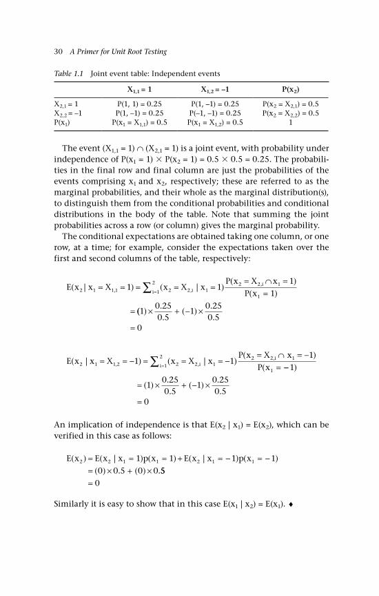
30 A Primer for Unit Root Testing
The event (X1,1 = 1) ∩ (X2,1 = 1) is a joint event, with probability under independence of P(x1 = 1) P(x2 = 1) = 0.5 0.5 = 0.25. The probabili-ties in the final row and final column are just the probabilities of the events comprising x1 and x2, respectively; these are referred to as the marginal probabilities, and their whole as the marginal distribution(s), to distinguish them from the conditional probabilities and conditional distributions in the body of the table. Note that summing the joint probabilities across a row (or column) gives the marginal probability.
The conditional expectations are obtained taking one column, or one row, at a time; for example, consider the expectations taken over the first and second columns of the table, respectively:
E x x X x X xP x X x
P xii
i( | ) ( | )( )
( ), ,,
2 1 1 1 2 2 11
2 2 2 1
1
1 11
1= = = = =
= ∩ ==
=
=∑
(( )..
( )..
10 250 5
10 250 5
0
× + − ×
=
E x x X x X xP x X x
P xii
i( | ) ( | )( )
(, ,,
2 1 1 2 2 2 11
2 2 2 1
1
1 11
= = − = = = −= ∩ = −
==∑ −−
= × + − ×
=
1
10 250 5
10 250 5
0
)
( )..
( )..
An implication of independence is that E(x2 | x1) = E(x2), which can be verified in this case as follows:
E x E x x p x E x x p x( ) ( | ) ( ) ( | ) ( )
( ) . ( ) .2 2 1 1 2 1 11 1 1 1
0 0 5 0 0
= = = + = − = −= × + × 55
0=
Similarly it is easy to show that in this case E(x1 | x2) = E(x1). ♦
Table 1.1 Joint event table: Independent events
X1,1 = 1 X1,2 = –1 P(x2)
X2,1 = 1 P(1, 1) = 0.25 P(1, –1) = 0.25 P(x2 = X2,1) = 0.5X2,2 = –1 P(1, –1) = 0.25 P(–1, –1) = 0.25 P(x2 = X2,2) = 0.5P(x1) P(x1 = X1,1) = 0.5 P(x1 = X1,2) = 0.5 1
Introduction to Probability and Random Variables 31
The order of the random variables in the conditioning affects none of the general principles. In example 1.6, the conditioning could have been taken as x1 on an event in the sample space of x2, thus the condi-tional probability would be written as P(x1 | x2), with conditional expec-tation E(x1 | x2). However, in the case of stochastic processes, there is a natural ordering to the random variables: x2 comes after x1 in the time series sequence, hence it is more natural to condition x2 on x1. This has relevance to a more formal approach to conditional expectations in which the –fields (or conditioning information sets) form an increas-ing nested sequence over time, see Section 1.8.
Example 1.7: A partial sum process
The example of Table 1.1 could be reinterpreted as simultaneously toss-ing two coins, and so time is not of the essence, therefore another process will serve to show the essential element of time-ordering and the sequen-tial nature of the kind of processes that are of interest in random walks and unit root tests. In a partial sum process, the order of the sequence, which is usually related to an index of time, is important. Consider a discrete-time stochastic process Y = (yt : 0 ≤ t ≤ T), then the corresponding partial sum process, psp, of Y is S = (St : 0 ≤ t ≤ T), where St = t
j=1yj, so that StT
t=1 = y1, y1 + y2, ..., Tj=1yj. The coin-tossing experiment is an example
of a psp provided that tosses of the coin are inherently consecutive and the random variable is that which keeps a running tally (sum) of the number of heads (or tails). Time is usually an essential aspect of a partial sum process and so the input random variable is referred to generically as yt, although when the input is white noise we set yt = t; where t is white noise (WN), defined by the properties: E(t) = 0; var(t) = 2 and cov(t s) = 0, for t ≠ s, see Chapter 2, Section 2.2.1.
The variance of St depends essentially on its ordered place in the sequence. Consider the variance of S2 : var(S2) = var(y1 + y2) = var(y1) + var(y2) + 2cov(y1, y2); if y1 and y2 are independent or there is no (serial) correlation, which is the weaker assumption, then cov(y1, y2) = 0, and, hence, var(S2) = 22
y. In general, var(St) = t2y, so that the variance of the
terms in the partial sum process are not constant and increase linearly with time. This example is considered further in example 1.9. ♦
1.7.2 Continuous random variables
The aim in this section is to generalise the concepts of independence, dependence and conditional expectation to the case of continuous ran-dom variables. The development is not completely analogous to the
32 A Primer for Unit Root Testing
discrete case because if the conditioning event is a single value it is assigned a zero probability and so an expression analogous to (1.41) would not be defined. To outline the approach, but to avoid this dif-ficulty in the first instance, we consider the conditioning event to have a non-zero probability.
Independence in terms of distribution functions is the condition that the joint distribution function factors into the product of the (marginal) distribution functions:
F X X F X F X( , ) ( ) ( )2 1 1 2 0− = (1.48)
In terms of density functions, the condition of independence is that the joint pdf factors into the product of the individual or marginal pdfs:
f X X f X f X( , ) ( ) ( )1 2 1 2 0− = (1.49)
These conditions are not problematical as assuming that the density functions exist then all component functions are well defined.
In seeking a conditional expectation, we could approach the task by first defining a conditional distribution function, by analogy with the discrete case, as the ratio of the joint distribution function to the (conditioning) marginal distribution function, or in terms of density functions as the ratio of the joint density function to the (condition-ing) marginal density function. As the density functions exist for the distributions considered in this book, we will approach the conditional expectation from that viewpoint.
1.7.2.i Conditioning on an event A ≠ a
In this section, the exposition is in terms of x2 conditional on x1. The problem to be considered is to obtain the probability of X2 B given that X1 A , the latter being the conditioning event, which is not a single element. This conditional probability is:
P X B X Af X A X B dX dX
f X A dX
X BX A
X A
( | )( , )
( )2 1
1 2 1 2
1 1 1
21
1
∈ ∈ =∈ ∈
∈∈∈
∈
∫∫∫
(1.50a)
Introduction to Probability and Random Variables 33
This notation is explicit but cumbersome and is sometimes shortened to:
P X B X Af X X dX dX
f X dX
X BX A
X A
( | )( , )
( )2 1
1 2 1 2
1 1
21
1
∈ ∈ = ∈∈
∈
∫∫∫
(1.50b)
The conditional pdf is given by:
f X B X Af X A X B
f X A( | )
( , )( )2 1
1 2
1
∈ ∈ =∈ ∈
∈ (1.51)
where A and B are Borel sets. Where the context is clear, the notation is simplified by omitting explicit reference to the sets, for example f(X2 | X1) = f(X1, X2)/f(X1) in place of (1.51).
The expression (1.51) is well defined provided that the denominator is positive, which we can ensure by setting A to be a nondegenerate interval, A = [A2 – A1] > 0. This rules out singletons, that is single points on the X1 axis; these are Borel sets, but lead to the problem that zero probability is assigned to such events for a continuous random variable. Graphically, the set B = [B2 – B1] ≥ 0 defines an interval on the X2 axis and the set A defines an interval on the X1 axis; their intersection is a rectangle.
A definition of the conditional expectation then follows as:
E x X A X f X X A dXX R x
( | ) ( | )( )2 1 1 2 1 2
2 2
∈ = ∈∈∫
(1.52)
If x1 and x2 are independent for all choices of sets in the event spaces of x1 and x2 then:
E x x X E x( | ) ( )2 1 1 2= = (1.53)
Example 1.8: The uniform joint distribution
To illustrate some of the key points so far, consider again the example of two (independent) random variables x1 and x2, with a uniform joint distribution, see example 1.3.
34 A Primer for Unit Root Testing
In this case the conditional probability function is:
P X B X A
A A B Ba a b b
A Aa a
dX( | )
( )( )( )( )
( )( )
2 1
2 1 2 1
2 1 2 1
2 1
2 1
1∈ ∈ =
− −− −
−−
ddX
B Bb b
X BX A 2
2 1
2 1
21
1
∈∈ ∫∫
= −−
≤( )( )
If we let B1 = b1, with B2 ≥ B1, then this defines a function that has the properties required of a conditional distribution function, so that we may write:
F X B X A P X B X A( | ) ( | )2 1 2 1∈ ∈ = ∈ ∈ (1.55)
Note that if B2 – B1 = 0 then F(X2 B | X1 A) = 0 and if B1 = b1 and B2 = b2 then F(X2 B | X1 A) = 1, as required in a probability measure. Independence is easily confirmed in this case: f(X1, X2) = f(X1)f(X2), f(X1 | X2) = f(X1), F(X1, X2) = F(X1)F(X2) and F(X2 B | X1 A) = F(X2 B).
A conditional expectation may also be defined as:
E x X A X f X X A dXb
b( | ) ( | )2 1 2 2 1 2
1
2∈ = ∈∫
(1.56)
In this illustration x1 and x2 are independent, so the conditional expec-tation reduces to:
E x X A X f X dX
E xb
b( | ) ( )
( )
2 1 2 2 2
1
1
2∈ =
=∫
(1.57)
for all B. ♦
1.7.2.ii Conditioning on a singleton
Although these definitions, for example (1.50) and (1.51), seem straight-forward extensions of the discrete random variable case, they raise a problem. From the start, the situation in which X1A f(X1)dX1 = 0 was ruled out, so that the set A could not be a single point in the range of X1 or a set with measure zero.
To see the problem, note that in the case of a discrete random vari-able, a conditional probability mass function is obtained by taking a
(1.54a)
(1.54b)
Introduction to Probability and Random Variables 35
value for, say, X1, as given; this fixes a row of the joint event table. Each cell entry in that row is then normalised by the sum of such entries, which necessarily results in each new probability being non-zero with a sum that is unity. The extension by analogy to a continuous random variable breaks down because the normalising factor is zero.
There are two ways forward. One is to redefine the conditional probabil-ity as a limit and the second is to go directly to the concept of a conditional expectation without first defining a conditional distribution or conditional density function. The solution outlined here is of the former kind and fol-lows Mittelhammer (1996); for an earlier reference see Feller (1966). The sec-ond approach is adopted in more advanced treatments, where the emphasis is on a measure-theoretic approach; the interested reader may like to con-sult Davidson (1994, chapter 10) and Billingsley (1995, chapter 6).
The idea taken here is to construct an interval set that shrinks to a single point in the limit; thus, let A = a ± , where ≥ 0, which collapses to a in the limit as → 0+. The conditional probability is now defined in terms of this limit as:
P X B X A P X B X a
f X X dX dXX
( | ) lim ( | )
lim( , )
2 1 0 2 1
0
1 2 1 21
∈ = = ∈ ∈ ±
=
→
→
=+
aa
a
X B
Xf X dX
f X X af X a
−
+
∈
= −
+
∫∫∫
==
=
2
11 11
1
2 1
1
( )
( , )( ))
( , )( )
dX
f X af a
dX
X B
X B
2
22
2
2
∈
∈
∫
∫=
The last line is just a matter of a shorthand notation. More substan-tively, the penultimate line follows from the mean value theorem for integrals and the continuity of f(X1) and f(X1, X2) in X1 for X1 A, see Mittelhammer (1996) for details. The difference between (1.50) and (1.58) is that, in the limit, there is no need for the integral over X1 A, because the set A collapses to a single point. The end result is simple enough and does have the same form as the discrete case. Thus, as (1.58) holds for all A, the conditional pdf, when conditioning on a singleton, is:
f X X af X X a
f X a( | )
( , )( )2 1
2 1
1
= = ==
(1.59)
(1.58a)
(1.58b)
(1.58c)
(1.58d)
36 A Primer for Unit Root Testing
where f(X1 = a) > 0. This means that we can go straight to the condi-tional expectation using this density:
E x X a X f X X a dXX R x
( | ) ( | )( )2 1 1 2 1 2
2 2
= = =∈∫
Moreover we may now take the expectation of the conditional expecta-tion by integrating out all possible values of a:
E E x X a
X f X X a dX f X dXX R xX R x
[ ( | )]
( | ) ( )( )( )
2 1
2 2 1 2 1 12 21 1
=
= =( )=
∈∈ ∫∫EE x( )2
(1.60)
The proof of the second line is left to a question, see Q1.4. The result states that taking the expected value conditional on the event X1 = a, and then weighting the resulting conditional expectations over all pos-sible values of X1 undoes the conditioning.
1.7.3 Independence in the case of multivariate normality
Multivariate normality is often important, for example in the properties of stochastic processes, so that a notation that allows the generalisation of the bivariate case will be worthwhile. Consider the random vector x = (x1, ..., xn) with expected value = (1, ..., n). The covariance matrix of x is the n x n matrix , where:
∑ =
−
−
12
2 1 1
2 1 22
2 1
1 2 12
, ,
, ,
, ,
n
n
n n n
(1.61)
is assumed to be non-singular (no linear dependencies among the n random variables) and ij is the covariance between variables i and j. The joint pdf is
f X X Xn( ) ( ) | | exp ( )’ ( )/ /= − − −
− − −212
2 1 2 1
(1.62)
where | | is the determinant of .

Introduction to Probability and Random Variables 37
A case of particular interest is when normal random variables are independent, in that case will be scalar diagonal and the joint pdf simplifies to:
f XXn
in
ii i
ii
n( ) ( ) ( ) exp/= − −
−=
−=∑2
12
21
1
1
2
(1.63)
where ni=1 is the product symbol. Also of interest in deriving maximum
likelihood based estimators is the log of the joint pdf. In the case of independent xi, the log of (1.63) is:
ln ( ) ( / )ln( ) lnf X nX
ii
n i i
ii
n= − − − −
= =∑ ∑2 2
121 1
2
(1.64)
1.8 Some useful results on conditional expectations: Law of iterated expectations and ‘taking out what is known’
This subsection outlines two results that are particular useful in analys-ing partial sum processes. The first is the law of iterated expectations (sometimes called the ‘tower’ property of expectations). The emphasis here is on the time series context. Consider the stochastic process (yt, 0 t T) generating Y = (y0, y1, ..., yT) and the following two conditional expectations: E(yt | F0
t–1) and E(yt | F0t–2), where F0
t–s = (yt–s, ..., y0) is regarded initially as an information set; then F0
t–2 F0t–1, thus F0
t–1 does not contain less information than F0
t–2, in this example the difference is the observation yt–1. Now consider the iterated expectation given by:
E E y E yt t[ ( | )| ] ( | )F F Ft t t0
10
20
2− − −= (1.65)
In effect the second (or outer) conditioning removes what information there is in F0
t–1 that is not in F0t–2, so that it has no effect. The iterating
can be continued. For example:
E E E ytt t t [ ( | ) | ]| ( | )F F F E y Ft
t0
10
20
30
3− − − −= (1.66)
This result holds because of the nested sequence of conditioning infor-mation. A more formal way of stating this result is in terms of –fields
38 A Primer for Unit Root Testing
rather than the concept of information sets. Thus, to reinterpret, let F0t–s
be the –field (yt–s, ..., y0), then F0t–2 F0
t–1, so that F0t–2 is a subfield of
Ft–1, then the law of iterated expectations states that:
E E y E yt t[ ( | )| ] ( | ]F F Ft t t0
10
20
2− − −= (1.67)
For a proof along general lines see, for example, Mikosch (1998).For the second property, start by considering the product of two ran-
dom variables, x and z. Then, in general, E(xz) ≠ E(x)E(z), equality hold-ing for independent random variables; however, if x is a constant then E(xz) = xE(z). There is an important case in the context of conditional expectations where, in the product of random variables one random variable can, in effect, be treated like a constant.
The general result is stated as follows, see for example Jacod and Protter (2004, Theorem 23.7), Mikosch (1998, Rule 5) and Davidson (1994, Theorem 10.10). Let x and z be random variables on the probabil-ity space (Ω, F, P), where x is measurable with respect to G, a –subfield such that G F, and assuming that x, z and xz are integrable, then:
E xz xE z( | ) ( | )G G= (1.68)
The intuition for the result is based on G F: x is known from the information in G and adds nothing to the information in F on z, it can, therefore, be treated as known and taken outside the expectation.
In a time series context, consider G = (yt–1, ..., y0) and F = (yt, ..., y0), then:
E y y y E yt t t t( | ) ( | )− −=1 1G G (1.69)
Because yt–1 is measurable with respect to G and G F, it can be treated as known in the conditional expectation.
1.9 Stationarity and some of its implications
At an intuitive level, stationarity captures the idea that certain proper-ties of a (data generating) process are unchanging. If the process does not change at all over time, it does not matter which sample portion of observations we use to estimate the parameters of the process; we may as well, therefore, use all available observations. On the other hand, this may be too strict a requirement for some purposes. There may be a break

Introduction to Probability and Random Variables 39
in the mean of the process, whilst the variance of the process remains the same. In that case, assuming that the mean is unchanging, which is a form of nonstationarity, is clearly wrong and will lead us into error; but rather than use only that part of the sample where the mean is constant, we may be able to model the mean change and use all of the sample.
The leading case of nonstationarity, at least in econometric terms, is that induced by a unit root in the AR polynomial of an ARMA model for yt, considered more extensively in Chapter 2. This implies that the variance of yt is not constant over time and that the k-th order autoco-variance of yt depends on t. This is, however, just one example of how nonstationarity can be induced.
Note that stationarity refers to a property of the process generating the outcomes – or data – that we observe; thus we should refer to a station-ary or nonstationary process, not to stationary or nonstationary data. Notwithstanding this correct usage, it is often the case that sample data is referred to as stationary or nonstationary. This is particularly so in the case of data generated from a stochastic process and presented in the form of a time series, when one finds a sample, for example data on GDP for 1950–2000, being referred to as nonstationary. This usage is widespread and does no particular harm provided that the correct meaning is understood.
1.9.1 What is stationarity?
Consider the coin-tossing experiment, where a single coin is tossed sequentially T times: what is the joint pmf for the resulting sequence Y = y1, y2, ..., yT, where y2 is the mapping H, T +1, –1? By inde-pendence, we can multiply together the pmfs for each P(yt) and as, by assumption, each of these is identical, the joint pmf is:
P y y y P yT tt
T( , , , ) ( )1 2 1
==∏
(1.70)
These assumptions mean that we can answer a number of elementary questions about sequence patterns. For example, what is the probability of the sequence (–1, +1, –1, –1, +1)? As P(–1) = P(+1) = 1–2, the answer is (1–2)5; indeed as the outcomes have equal probabilities, all outcome sequences for a given T are equally likely, and as there are 25 possible sequences, each equally likely, then the probability of each must be 2–5 = (1–2)5.
Suppose we wanted to assess the assumption that the two outcomes for each t were, indeed, equally likely. Now the order in the sequence is not vital, so that one line of enquiry would be to count the number of –1 (or +1) outcomes in the sequence and divide by the number in the
40 A Primer for Unit Root Testing
sequence. This uses the ‘outcome’ average to estimate the probability P(yt = –1), say P = #I(–1)/T, which is the number of observed occurrences of –1 divided by T, where I(–1) = 1 if the outcome is –1 and 0 otherwise, and # indicates the counting operator. This is a sensible estimator given that the probability structure over the sequence is unchanging (see Chapter 3, Section 3.3 on ergodicity).
However, suppose that the coin-tossing ‘machine’ develops a fault and P(yt = –1) becomes more likely from a point halfway through the sequence; then the time average is misleading due to the change in the underlying structure. In this case, it is necessarily the case that the mean and the variance of the process have changed; that is key elements of the underlying probability structure are not constant or ‘stationary’. This illustration uses the independence property explicit in the random experiment of coin tossing, but it is not a part of the definition of sta-tionarity. The next two subsections show what is required depending on the particular concept of stationarity.
1.9.2 A strictly stationary process
Let ≠ s and T be arbitrary, if Y is a strictly stationary, discrete-time process for a discrete random variable, yt, then:
P(y+1, y+2, ..., y+T) = P(ys+1, ys+2, ..., ys+T) (1.71)
That is, the joint pmf for the sequence of length T starting at time + 1 is the same for any shift in the time index from to s and for any choice of T. This means that it does not matter which T-length portion of the sequence we observe. Since a special case of this result in the discrete case is for T = 1, that is P(y) = P(ys), the marginal pmfs must also be the same for ≠ s implying that E(y) = E(ys). These results imply that other moments, including joint moments, such as the covariances, are invari-ant to arbitrary time shifts.
If the random variables are continuous and defined in continuous time, a strictly stationary random process must satisfy the following:
F y t y t y t F y s t y s t y s tT T( ( ), ( ), , ( )) ( ( ), ( ), , ( )) + + + = + + +1 2 1 2 (1.72)
where t1 < t2 ... < tT, ≠ s and F(.) is the joint distribution function. If the probability density functions exist, then an analogous condition holds, replacing F(.) by f(.):
f y t y t y t f y s t y s t y s tT T( ( ), ( ), , ( )) ( ( ), ( ), , ( )) + + + = + + +1 2 1 2 (1.73)
Introduction to Probability and Random Variables 41
An iid stochastic process, as in the example opening this section, is strictly stationary.
1.9.3 Weak or second order stationarity (covariance stationarity)
A less demanding form of stationarity is weak or second order stationar-ity, which requires that the following three conditions are satisfied for arbitrary and s, ≠ s:
SS1. E(y) = E(ys) = SS2. var(y) = var(ys) = 2
SS3. cov(y, y+k) = cov(ys, ys+k)
The moments in SS1–SS3 are assumed to exist. The first condition states that the mean is constant, the second that the variance is con-stant and the third that the k-th order autocovariance is invariant to an arbitrary shift in the time origin. The extension to continuous time is straightforward, replacing y by y() and so on. From these three conditions, it is evident that a stochastic process could fail to be weakly stationary, because at least one of the following holds over time:
i. its mean is changing; ii. its variance is changing;iii. the k-th order autocovariances depend on time for some k.
A stochastic process that is not stationary is said to be nonstationary. A nonstationary process could be: nonstationary in the mean; nonsta-tionary in the variance; and/or nonstationary in the autocovariances. Usually it is apparent from the context whether the stationarity being referred to is strict or weak. When the word stationary is used with-out qualification, it is taken to refer to weak stationarity, shortened to WS, but, perhaps, most frequently referred to as covariance stationarity. (Weak or covariance stationarity is also referred to as wide-sense sta-tionary, leading to the initials WSS.)
Ross (2003) gives examples of processes that are weakly stationary but not strictly stationary; however, note that, exceptionally, a process could be strictly stationary, but not weakly stationarity by virtue of the non-existence of its moments. For example, a random process where the components have unchanging marginal and joint Cauchy distribu-tions will be strictly stationary, but not weakly stationary because the moments do not exist.

42 A Primer for Unit Root Testing
Example 1.9: The partial sum process continued (from Example 1.7)
An example of a process that is stationary in the mean, but nonstation-ary in the variance, is the partial sum process (introduced earlier in example 1.7) with iid inputs, as in the case of Bernoulli or white noise inputs. If the process starts at j = 1, then St = t
j=1 yj, with E(yj) = 0, and E(St) = t
j=1 E(yj) = 0. The variance of St is given by:
var( ) var
( )
S y
E y E y j
t
t jj
t
jj
t
j
y
= ( )= ( ) =
= +
=
=
∑
∑1
1
2
2
0
2
using for all
ccov( , ) var( )y y y i
t
i jj i
t
i
t
j y
y
>= ∑∑ =
=1
2
2
using for all
(1.74)
where the last line uses using cov(yi, yj) = 0. In passing note that this result only requires that the sequence yt is white noise rather than iid (hence we could have written yt = t).
From (1.74) note that the variance is not constant and the partial sum process is, therefore, nonstationary in the variance. The process also becomes nonstationary in the mean if E(yj) = µ ≠ 0 as when E(St) = t, as well as var(St) = t2
y. Finally, Sjtj=1 is also nonstationary in the autocov-ariances, even if cov(yi, yj) = 0 for i ≠ j. To illustrate consider the follow-ing two first-order autocovariances, cov(S1, S2) and cov(S2, S3), then:
cov( , ) cov( , )
cov( , )
cov( , ) cov(
S S y y y
y y
S S y y
y
1 2 1 1 2
21 2
2 3 1
= +
= +
= +
22 1 2 3
21 2 1 3 2 32 2
, )
cov( , ) cov( , ) cov( , )
y y y
y y y y y yy
+ +
= + + +
These differ, although both refer to a first order autocovariance; hence, the process is nonstationary as the translation in time does affect the joint probability mass function.
1.10 Concluding remarks
This chapter has introduced a number of concepts and some language and terminology that are vital to later chapters. One cannot make sense of random walks and Brownian motion without a background knowl-edge of probability or of, for example, memory and persistence in a stochastic process without the concept of dependence. The partial sum
Introduction to Probability and Random Variables 43
process is critical to not only random walks and Brownian motion but also to the development of the distribution theory of unit root tests.
There are a number of excellent texts on probability and stochastic processes that can serve as a follow up to this chapter. On probability, these include Larson (1974), Fristedt and Gray (1997), Jacod and Protter (2004), Koralov and Sinai (2007), Ross (2003) and Tuckwell (1995); a classic, but advanced, reference on the measure theory approach to probability is Billingsley (1995) and Feller’s (1966, 1968) two volumes on probability theory are classic and timeless texts. On stochastic proc-esses see, for example, Brzezniak and Zastawniak (1999), Mikosch (1998) and Stirzaker (2005). Classic texts on stochastic processes include Doob (1953) and Cox and Miller (1965); and Karlin and Taylor’s (1975a, 1975b) two volumes on stochastic processes provide an excellent graded intro-duction and development of a great deal of relevant material.
Questions
Q1.1 Suggest some possible examples of random variables from every-day life and state whether the random variable so defined is discrete or continuous.
A1.1 The time you wake in the morning (continuous); the number of arrivals at the supermarket checkout in given interval of time (discrete);
Q1.2 Consider a random experiment where a fair coin is tossed ten times and the number of times that the coin lands heads is noted. A student argues that since the coin is fair, the probability of 5 heads out of 10 is ½. Is he correct?
A1.2 First note that this is a Bernoulli trial with n = 10 and probability of success P(H) = p = ½ and q = 1 – p = ½, and let k denote the number of heads. There are various ways that k = 5 can occur, for example, the coin lands heads on the first 5 throws and then tails on the next 5; it lands tails on the first throw and then lands heads on the next 5 followed by 4 tails. Each of these outcomes taken individually has a probability of occurrence of pkq(n–k); with n = 10, k = 5 and p = ½, this probability is 1–2
5 1–2
(10–5) = 1–210.
However, we also need to consider how many ways 5 heads can occur in 10 tosses. To do this we need the number of ways that we can choose k from n without regard to order, this is the combinatorial factor nCk = n!/ [(n – k)!k!], where n! = n(n – 1) ... 1, read as n factorial. The required prob-ability is then nCkpkq(n–k) = nCkpn; for n = 10, k = 5 and p = ½, 10C5p5q5 = 252 (1–2)5 = 0.2461; the student is wrong! (This example is due to Bean, 2009.)
Q1.3 Let C = (A, B) where A, B Ω: generate the –field of C, denoted (C).

44 A Primer for Unit Root Testing
A1.3 The first condition for a –field requires that , Ω be in (C); then include all unions and unions of complements, A ∪ B, Ac ∪ B, A ∪ Bc and Ac ∪ Bc; therefore, (C) = (, A ∪ B, Ac ∪ B, A ∪ Bc, Ac ∪ Bc, Ω).
Q1.4 Show that in both the discrete and continuous cases E[E(x1 | X2)] = E(x1).
A1.4 Consider the discrete case first as it will provide a clue for the con-tinuous case. We want to evaluate the expectation of the conditional expectation:
E E x x X E x x X p x X
Xp x X
i i ii
n
j
[ ( | )] ( | ) ( )
(
, , ,
,,
1 2 2 1 2 2 2 21
11 1
= = = =
==
=∑jj i
ij
m
ii
n
j
x X
p x Xp x X
X p x X
∩ ==
=
= =
== ∑∑ 2 2
2 21 2 21
1 1
,
,,
,
)
( )( )
( 11 2 211
1 1 11
1
, ,
, ,
)
( )
( )
j ii
n
j
m
j jj
m
x X
X p x X
E x
∩ =( )= =( )=
==
=
∑∑∑
The second line follows by substitution for the conditional expectation and the conditional probability; the third line follows by cancellation of p(x2 = X2,i); the summations are interchanged in the fourth line, then the sum over all joint probabilities (that is one row or column of the joint event table) results in the marginal probability.
In the case of a continuous random variable, the starting expression is:
E E x X b X f X X b dX f X dXX R xX R x
[ ( | )] ( | ) ( )( )( )1 2 1 1 2 1 2 2
1 12 2
= = =( )=
∈∈ ∫∫
XXf X X b
f X bdX f X dX
X
X R xX R x 11 2
21 2 2
1
1 12 2
( , )( )
( )( )( )
==
=
∈∈ ∫∫ff X X b
f X bf X dX dX
X f
X R xX R x
( , )( )
( )
(
( )( )
1 2
22 2 1
1
2 21 1
==
=
∈∈ ∫∫
XX X b dX dX
X f X dX
E
X R xX R x
X R x
1 2 2 1
1 1 1
2 21 1
1 1
, )
( )
(
( )( )
( )
=( )=
=
∈∈
∈
∫∫
∫xx1)
The line operations are analogous to the discrete case; of note is the integrating out of the conditioning event such that
X2R(x2) f(X1, X2 = b)
dX2 = f(X1).
2Time Series Concepts
45
Introduction
This chapter brings together a number of concepts that are essential in characterising and analysing time series models. The reader is likely to be familiar with series of observations that are ordered by time and arranged into a sequence; for example quarterly observations on GDP from 1950q1 to 2009q4 (T = 240 observations). In practice we observe one set of observations, but conceptualise these as outcomes from a process that is inherently capable of replication. In order to do this, each sample point of the 240 is viewed as an outcome, or ‘draw’, from a random variable; there are, therefore, in the conceptual scheme, 240 random variables, arranged in a sequence, Y = (y1, y2, ..., y240), each with a sample space corresponding to the multiplicity of possible outcomes for each random variable, and a sample space for the entire sequence. In Chapter 1, this sequence was referred to as a stochastic process, where an outcome of such a process is a path function or sample path, not a single point.
This chapter proceeds as follows. The lag operator is introduced in Section 2.1; its many uses include obtaining the autocovariance generat-ing function, measuring persistence, obtaining impulse response func-tions, finding the roots of dynamic models and calculating mean lags. The ARMA model, which is central to many unit root tests, is outlined in Section 2.2. As a key preliminary in this chapter is characterising the degree of dependence, autocovariances, autocorrelations and variances are introduced in Section 2.3; this section also includes an introduction to the long-run variance. Section 2.4 is concerned with some simple, but widely used, tests for dependence. One use of the lag operator, that is in defining the autocovariance generating function, ACGF, is dealt
46 A Primer for Unit Root Testing
with in Section 2.5. Estimation of the long-run variance is considered in 2.6; and Section 2.7 includes some empirical examples. Throughout this chapter, time is of the essence and, therefore, the adopted notation is of the form for a discrete-time random variable.
2.1 The lag operator L and some of its uses
The lag operator is an essential tool of time series econometric analysis. We outline some basic principles in this subsection; a more extensive discussion can be found in Dhrymes (1981).
2.1.1 Definition of lag operator L
The lag operator, sometimes referred to as the backshift operator, is defined by:
L y yjt t j≡ − (2.1)
A negative exponent results in a lead, so that:
L y y yjt t j t j
−− − +≡ =( ) (2.2)
Lag operators may be multiplied together as follows:
L L y yj it t j i≡ − +( ) (2.3)
Setting j = 0 in Ljyt leaves the series unchanged, thus L0yt yt, and L0 1 can be regarded as the identity operator. If the lag operator is applied to a constant, the constant is unchanged; that is, Lj , where µ is a constant.
In the backshift notation, often preferred in the statistics literature, the notation for the lag operator is B, thus Bjyt yt–j. The lag operator is more than just a convenience of notation; it opens the way to write functions of the lags and leads of a time series variable that enable some quite complex analysis.
2.1.2 The lag polynomial
A polynomial in L can be defined using the lag operator notation, thus (L) = 1 – p
j=1jLj; for example, the second order lag polynomial is (L) = 1 – 1L – 2L2. Note that this is a special form of the polynomial
Time Series Concepts 47
(L) = 0 – 1L – 2L2 , with 0 = 1. The lag polynomial can be applied to the random variable yt at time t, as well as to the sequence of random variables yt t
t T==1 to obtain a new sequence. In the case of the second
order polynomial (L)yt (1 – 1L – 2L2)yt yt – 1yt–1 – 2yt–2 and this
operation defines a new random variable, which is a linear combination of yt, yt–1, and yt–2; when applied to yt
Tt=1 a new sequence of random
variables is defined.
2.1.3 Roots of the lag polynomial
Writing the lag structure using the lag operator enables some simple algebraic operations, but we have to be careful not to use the lag opera-tor L both as an operator and a variable, which would contradict its definition (2.1). Instead, the variable z takes the place of the operator L and the analysis is pursued in terms of (z). For example, the first order polynomial is written as (z) = 1 − 1z. To obtain the root of this poly-nomial involves solving for the value of z such that (z) = 0; the solution is z = 1/1, which gives rise to the terminology that (z) has the root 1/1, which is a unit root if 1 = 1.
At this point, it is useful to clarify a distinction in approach that arises in connection with the roots of polynomials. Note that nothing funda-mental changes in seeking the solutions (zeros) of (z) = 0 on dividing the lag polynomial through by the coefficient on zp; it implies that zp has a coefficient of unity, but the solutions are unchanged. The benefit is a neater way of representing the roots. In the case of a quadratic lag polynomial, the form of the factorisation is (z − 1)(z − 2) = 0, and 1 and 2 are the two roots of this quadratic. This approach and factorisation separates the use of variable z from the roots i and is a preferable nota-tion. This procedure generalises in a straightforward manner: let (z) = 1 – p
j=1 jzj, then the polynomial factors as pi=1 (z – i) = 0, where i i =
1, . . . , p are the p roots of (z). Notice that if one or more of the roots is unity, then (1) = 0, where (1) is shorthand for (z) evaluated at z = 1, so that (1) = 1 – p
j=1 j.The inverse of the lag polynomial, if it exists, is defined such that
(L)–1 (L) = 1, and the lag polynomial is said to be invertible. Consider the first order polynomial (L) = 1 − 1L and note that provided | 1 | < 1 the inverse of this polynomial can be defined; in this case (1 – 1L)–1 (1 – 1L) = 1, where (1 – 1L)–1 = 1 –
j=1 1jLj and convergence of the infinite
sum is assured by the condition | 1 | < 1. More generally the condition that ensures invertibility is that the roots of the lag polynomial have moduli greater than unity, | i | > 1, said to be ‘outside the unit circle’.

48 A Primer for Unit Root Testing
Example 2.1: Roots of a second order lag polynomial
Obtain the roots of the lag polynomial yt – 1.25yt–1 + 0.25yt–2 and check for invertibility. The roots are the solutions to 1 – 1.25z + 0.25z2 = 0. Divide the lag polynomial through by 0.25 to obtain (z) = 4 – 5z + z2 = 0, which factors as (z − 1)(z − 4) = 0. This is an example of (z − 1)(z – 2) = 0, so that the roots are 1 = 1 and 2 = 4. The lag polynomial is not invertible because one root, 1, is on the unit circle. Note that isolating the unit root and rewriting the lag polynomial in terms of the remain-ing root, results in an invertible polynomial, specifically: yt – 1.25yt–1 + 0.25yt–2 = (1 – L)yt – (1 – L)0.25Lyt and, as usual, define yt (1 – L)yt, so that the polynomial is yt – 0.25Lyt, and the polynomial (1 – 0.25L) is invertible, indeed we know that, by construction, it has one root = 4.
2.2 The ARMA model
The autoregressive, moving average model is a special but important case of a linear process relating yt to stochastic inputs. It features widely in tests for a unit root, which in effect focus on the AR component of the model. This section outlines some important features of this class of model; and subsequent sections use some simple ARMA models for illustration. References to follow up this important area of time series analysis are given at the end of the chapter.
2.2.1 The ARMA(p, q) model using lag operator notation
The lag operator notation allows an economic way of writing the familiar ARMA(p, q) model, where p and q refer to the lag lengths on the AR and MA components of the model, respectively. The ARMA(p, q) model is:
y yt i t ii
p
t j t jj
q= + +−= −=∑ ∑
1 1
(2.4)
The AR part of the specification refers to the lags on yt and the MA part to the lags on t; these are p and q, respectively. For simplicity the speci-fication in (2.4) implicitly assumes E(yt) = 0, if this is not the case, say E(yt) = µt, then yt is replaced by yt – µt, in which case (2.4) becomes:
y yt i t ii
p
t j t jj
q= + +−= −=∑ ∑
1 1
(2.5)
where y~t = yt – µt. The two most familiar cases are µt = µ and µt = 0 + 1t. The usual procedure in these cases is to replace µt by a consistent
Time Series Concepts 49
estimator; in the former case, µ is usually estimated by the sample mean and in the latter case 0 and 1 are estimated by a LS regression of yt on a constant and t (with ^ over indicating an estimator) and y~t = yt – µt, where µt = 0 + 1t, is referred to as the detrended data. In the case of a trend other methods are available see, for example, Canjels and Watson (1997) and Vogelsang (1998).
It is usual to add a specification of t to complete the ARMA model, and we digress briefly to cover this point. The intention of the speci-fication is to ensure that the t, t = 1, . . . , T, are not serially dependent. However, there are various ‘strengths’ of the assumptions that can be made. To understand these we start with the assumption that t is white noise (WN), defined as: E(t) = 0; var(t) = 2, a constant for all t; and cov(ts) = 0, for t ≠ s, that is the (auto)covariance between t and s
is zero. A slightly stronger version of white noise (strong or independ-ent white noise) is to specify that the sequence, t
Tt=1 comprises t that
are independently and identically distributed (iid) for all t, written as t ~ iid(0, 2). Normality of t is not an essential part of either of these specifications; if it assumed then we write t ~ niid(0, 2), so that the t
are independent not just uncorrelated. Another possibility requires us to look ahead to a martingale difference sequence (MDS), see Chapter 3, Section 3.5.1. For present purposes, we note that an MDS allows some heteroscedasticity, and we may alternatively specify that t is a stationary MDS with finite variance. Our default assumption is that t ~ WN(0, 2), with the notational convention that t and 2 are gener-ally reserved for this specification. Hayashi (2000) shows that in terms of increasing strength of assumptions, the relationships are: white noise MDS strong white noise.
Returning to the main issue, in terms of lag polynomials, the ARMA(p, q) model is written as one of the following:
( ) ( )L y Lt t= (2.6a)
( ) ( )L y Lt t= (2.6b)
where ( ) , ( ) ~ ( , ).L L L L WNii
i
p
jj
j
q
t= − = += =∑ ∑1 1 0
1 1
2and
Example 2.2: ARMA(1, 1) model
The specification of this model is:
( ) ( )1 11 1− = + L y Lt t
50 A Primer for Unit Root Testing
The polynomial (1 – 1L) has an inverse provided that | 1 | < 1, so that the model is invertible. Multiplying through by the inverse polynomial results in:
y L L
L L
L
t t
j
j t
= − +
= +( ) +
= + + +
−
=
∞∑( ) ( )
( )
( )
1 1
1 1
1
11
1
11 1
1 1 1
(( ) ( )
1 12
1 13
0
+ + +( )=
=
∞∑L L
L
t
jj
j t
12
where 0 = 1 and j = 1j–1(1 + 1) for j ≥ 1. This is the MA(∞) representa-
tion of the original ARMA(1, 1) model. ♦The polynomials (L) and (L) in Equation (2.6) are assumed to have
no roots in common. To give a counter-example suppose that it was the case in the ARMA(1, 1) model (1 – 1L)yt = (1 + 1L)t, that 1 = –1, then the polynomials would cancel to leave yt = t. In practice, such exact cancellation is rare, but near-cancellation does occur especially as p and q are increased.
At this point, it is worth pointing out a departure from the notation of Equation (2.4) in the case of the AR(1) model. It is conventional in the area of unit root tests to adopt the notation that rather than 1 is the coefficient on yt–1, so that the commonplace (and equivalent) nota-tion is yt = yt–1 + t. This simple model, or a slight generalisation of it, is an often used vehicle for unit root tests. In fact, this notational conven-tion has a substantive base in terms of the formulation of a model for unit root testing, see Chapter 8.
2.2.2 Causality and invertibility in ARMA models
An ARMA(p, q) model is described as being causal if there exists an absolutely summable sequence of constants j0
, such that:
y L
L
t jj
tj
t
=
==
∞∑
0
( ) (2.7)
The condition of absolute summability is j=0 |j| < ∞. The lag poly-
nomial (L) is the casual linear filter governing the response of yt to t. The representation in (2.7) is the MA form of the original model, which will be MA(∞) if (L) is not redundant. The MA polynomial is
Time Series Concepts 51
(L) = j=0 jLj = (L)–1 (L), with 0 = 1; for this representation to exist
the roots of (L) must lie outside the unit circle.The MA form (2.7) provides the basis of a number of tools of interpre-
tation of the original model. A measure of persistence based on (2.7) is considered in Section 2.2.3, and Section 2.6 considers the related con-cept of the long-run variance.
Note that (2.7) defines a linear filter since yt is expressed as an additive function of current and past values of t. Provided that (L) is invert-ible, the ARMA model of (2.4) necessarily implies a linear filter of the form in (2.7); however, one could start an analysis by assuming that yt was generated by a linear filter, without necessarily specifying that the filter was generated by an ARMA model; for an application of this idea in the context of unit root tests, see Phillips and Solo (1992).
Although the condition of causality requires the invertibility of (L), the term invertibility is more usually taken to refer to the MA polynomial in the ARMA model. That is suppose (L)–1 exists, then the ARMA(p, q) model has the invertible representation:
( )L yt t= (2.8a)
where (L) = j=0 jLj = (L)–1 (L) and 0 = 1. Thus (2.8a) may be written
explicitly in infinite AR form as:
y L y
L y
t t t
jj
tj t
= − +
= − +=
∞∑[ ( )]1
1
(2.8b)
Analogous to the condition on (L), the representation in (2.8) requires that the roots of (L) lie outside the unit circle and that the sequence of coefficients in (L) is absolutely summable, that is
j=0 | j | < ∞. Consider the MA(1) case. Then yt = (1 + 1L)t and invertibility requires that the following representation exists:
(L)yt = t
where (L) = (1 + 1L)–1; provided that | 1 | < 1, then the inverse exists and is given by:
( ) ( )1 1 111
10+ = + −−
=
∞∑ L Lj j j
j
52 A Primer for Unit Root Testing
This example illustrates the general condition that the modulus of the root(s) of the MA polynomial must lie outside the unit circle for the ARMA model to be invertible.
It is usual to impose an invertibility condition on the MA polynomial to ensure identifiability of the MA coefficients. This is because differ-ent sets of MA coefficients give rise to the same autocorrelation struc-ture. The problem can be illustrated most simply with the MA(1) model. The first order autocorrelation coefficient 1 (defined in Section 2.3.1, below), for this case is exactly the same if 1
–1 replaces 1, that is:
y L
y L
t t
t t
= + ⇒ =+
= + ⇒ =+
−
( )( )
( )/
( ( / ) )
11
11
1 1
1 11
12
11
11
12
==+
=+
11 11 1
212
1
12
( )/ ( )
However, whilst 1 is unchanged, the root of (1 + 1L) is –1/1, whereas the root of (1 + 1
–1L) is –1 and, if |1| < 1 then only the first of these polynomials is invertible. Given that 1 can be mapped back into differ-ent sets of MA coefficients then imposing invertibility ensures that one particular set is chosen (or identified).
2.2.3 A measure of persistence
The idea here is to determine the effect on yt of a unit increase in t
which, when calculated as the total effect, is one measure of the per-sistence embodied in the model. The moving average representation of (2.7) is the most efficient way to obtain the required quantities.
For illustrative purposes, initially assume that (L) is the second order polynomial given by:
yt = t + 1t–1 + 2t–2
The (finite) order of (L) will be denoted S, so in this case S = 2. Now consider a one unit one-off shock at time t; this can be represented as *t+s = t+s + 1 for s = 0, and *t+s = t+s for s ≥ 1. This shock will trace through time as follows:
y y
y y
y
t t t t
t t t t t
t
+−
++
+ − +
+
= + + = +
= + + + = +
1 1
11 1
1 1 1 2 1 1 1
2
( )++
+ + +
++
+
= + + + = +
= ≥
t t t t
t s t s
y
y y s2 1 1 2 2 21
2
( )
for

Time Series Concepts 53
From this pattern, we can infer that y+t+s – yt+s = s for s ≤ S and y+
t+s – yt+s = 0 for s > S. Evidently, the lag coefficients in the moving average repre-sentation capture the differences due to the unit shock.
If the shock is sustained, that is *t+s = t+s + 1 for s ≥ 0, then following through the pattern over time, we can establish that y+
t+s – yt+s = sj=0 j
for s < S, and y+t+s – yt+s = S
j=0 j for s ≥ S. So, in this case, it is the partial sum of the lag coefficients that capture the sustained one unit shock if s < S and the sum of the lag coefficients if s ≥ S. The sum S
j=0 j is a measure of persistence, in that it shows how much y+
t+S differs from yt+S.Increasing S, for example letting S → ∞, does not change any aspect
of principle outlined here. Thus, the limiting (or long-run) effect of a sustained one unit shock, where (L) is a lag polynomial of infinite order is:
( ) lim∞ = →∞ =∑S jj
S
0 (2.9)
To put this another way limS→ (y+t+S) = yt+S + (), so that in the limit
yt+S and yt+S differ by (). It is for this reason that () can be inter-preted as a measure of persistence; for example, suppose that () = 0, then the sustained unit shock has no effect in the long run. To illustrate the other extreme, consider the AR(1) model given by yt = yt–1 + t; provided that || < 1, then this has the infinite MA representation yt = (1 – L)–1 t . That is:
y L
L L
L L
t t
t
t
= −
= + + +
= + + +
−( )
( )
( )
1
1
1
2 2
0 1 22
where 0 = 1 and j = j for j ≥ 1. From the definition of persistence, we obtain (S) = 1 + S
j=1 j = 1 + Sj=1
j and hence: () = 1 + j=1
j = (1 – )–1
Note that as → 1, then () → ∞. Thus as the unit root is approached, persistence, as measured by (), increases without limit. This result generalises: all that is required is that the AR polynomial includes at least one unit root.
Finally, () can be obtained very simply on noting that it is the (lim-iting) sum of the moving average coefficients, but rather than working out the sum, which could be tedious, it can be obtained by setting z = 1
54 A Primer for Unit Root Testing
in the MA lag polynomial w(z). That is:
( ) ( | )
|
∞ = =
= =( )=
=
∞
=
∞
∑∑
z z
z zjj
j
jj
1
10
0
(2.10)
The shorthand notation for (z | z = 1) is (1), see also Section 2.1. Moreover if (1) is a rational polynomial, as in the invertible ARMA model, then () is obtained by setting L = 1 in each component poly-nomial, thus:
( ) ( )( )( )
∞ = =
1
11
(2.11)
Example 2.3: ARMA(1, 1) model (continued)
In the case of the ARMA(1, 1) model of example 2.1, the persistence measure () is:
( ) ( )( )( )
∞ = = +−
1
11
1
1
For example, if 1 = −0.3 and 1 = 0.9, then () = 7. This calculation is clearly much more efficient than computing the infinite sum using j
as determined in example 2.2. ♦
2.2.4 The ARIMA model
The case of a unit root in the AR component of an ARMA model is sufficiently important to separate it from the general case. By way of motivation, consider the ARMA(2, 0) model, with the lag polynomial of example 2.1, that is:
( . . )1 1 25 0 25 2− + =L L yt t
so that (L) = (1 – 1.25L + 0.25L2). The roots of (L) were obtained as 1 = 1 and 2 = 4, so (L) is not invertible. However, the AR polynomial is invertible if the variable is redefined to include the unit root, that is (L)yt = (p–1)(L)yt, where (p–1) is of one lower order than (L). In
Time Series Concepts 55
example 2, we saw that (p–1) = (1 – 0.25L), which is invertible. In this
case, there is d = 1 unit root, which can be extracted to leave an invert-ible polynomial.
This idea generalises, so that if there are d ≥ 1 unit roots, then:
( ) ( ) ( ) ( )( )L y L L y Lt tp d d
t t= ⇒ =− (2.12)
where (p–d) is an invertible polynomial and d (1 – L)d is the d-th
differencing operator, which necessarily has d unit roots. The result-ing model is described as an autoregressive integrated moving aver-age model, ARIMA(p − d, d, q), which corresponds to the underlying ARMA(p, q) with d unit roots in the AR polynomial. Sometimes the ARIMA model is written as ARIMA(p, d, q), in which case the underly-ing ARMA model is ARMA(p + d, q).
When yt is generated by an ARIMA(p − d, d, q) process, it also inte-grated of order d, written yt ~ I(d), in that modelling in terms of the d-th difference of yt results in a casual (AR invertible) and stationary model. The most familiar case is d = 1, that is yt ~ I(1), so that the unit root is accommodated by modelling yt rather than yt. The concept of an inte-grated process is intimately related to the concept of stationarity, which was considered in Chapter 1, Section 1.9 and is considered further in Chapter 3, Section 3.2.
2.3 Autocovariances and autocorrelations
This section introduces a number of basic building blocks with which to analyse time series. A key aspect in characterising a time series is the extent of its dependence on itself, usually referred to as serial depend-ence, and for linear time series, the basic concept is the autocovariance, considered in the next section.
2.3.1 k-th order autocovariances and autocorrelations
The k-th order autocovariance is a measure of the (linear) dependence between yt and its k-th lag, yt–k (equivalently, the k-th lead, if the proc-ess generating the data is covariance stationary, see Chapter 1, Section 1.9 and Chapter 3, Section 3.2). It is defined as:
k t t t k t kE y E y E y E y k= − − = ±− −( ) ( ( ) , , ,...1 2 3 (2.13)

56 A Primer for Unit Root Testing
For k = 0, 0 is the variance, given by:
02= −E y E yt t ( ) (2.14)
Notice that if E(yt) = 0 for all t, then 0 = E(yt2 ) and k = E(ytyt–k).
The k-th order autocorrelation coefficient k is k scaled by the vari-ance, 0, so that:
k
k=0
(2.15)
The scaling ensures that 0 ≤ | k | ≤ 1. A word on notation at this point: k
is the conventional notation for the autocorrelation coefficient, which we have followed here – it will always have a subscript; , without a subscript, is the notation reserved for the coefficient on yt–1 in the AR(1) model. Considered as a function of k, k and k give rise to the autocov-ariance and autocorrelation functions; the latter portrayed graphically, with k on the horizontal axis and k on the vertical axis, is referred to as the correlogram.
The existence of k and k requires that E(yt–k) exists. There are some distributions for which this is not the case; for example, these expecta-tions do not exist for the Cauchy distribution, a feature that arises intui-tively because the ‘fat’ tails of the Cauchy imply that there is ‘too’ much probability mass being applied to outlying realisations and, as a result, the weighted integral in E(yt) does not converge to a finite constant.
The autocovariance function of pure MA processes, which are just linear combinations of white noise (and hence uncorrelated) inputs, are particularly easy to obtain. These are as follows, where yt = (L)t, with (L) = 1 + q
j=1jLj, t ~ WN(0, 2) and finite q, then we have:
02 2
0=
=∑ jj
q
(2.16a)
k j j kj
q kk q= =+=
−∑2
01| |
| |,...,for
(2.16b)
where 0 = 1. It then follows that the autocorrelations are given by:
k j j kj
q k
jj
q= +=
−
=∑ ∑| |
| |
0
2
0 (2.17)
Time Series Concepts 57
For example:
q k
qk k= = + = = + = = ≥
=
1 1 1 0 2
20 1
2 21 1
21 1 1
2, ( ) , , /( ), ;
,
for
0 12
22 2
1 1 2 12
2 22
1 1 2 1
1
1
= + + = + =
= + +
( ) , ( ) , ;
( )/( 112
22
2 2 12
221 0 3+ = + + = = ≥ ), /( ), .k k kfor
In the case of MA processes that result from the inversion of a casual ARMA model, then the MA coefficients are denoted j, which is the j-th coefficient of (L). The autocovariances and autocorrelations are then given by:
02 2
0=
=
∞∑ jj (2.18a)
k j j kj= +=
∞∑2
0 | | for k ≥ 1
(2.18b)
k j j kj jjfor k= ≥+=
∞
=
∞∑ ∑2
0
2
01| |
(2.18c)
An example is given below, see example 2.4. An alternative method of obtaining the autocovariance and autocorrelation functions is by way of the autocovariance generating function, see Section 2.5.
2.3.2 The long-run variance
It is also useful at this stage to introduce the concept of the long-run variance, which is the limiting value as T → ∞ of var( )Ty , denoted 2
lr,y. Consider the following:
lr y T
T tt
T
T
Ty
T y
T y
,
/
lim var
lim var
lim var
2
1 2
1
1
= ( )= ( )=
→∞
→∞−
=
→∞−
∑ttt
T
=∑( )1
(2.19)
Notice the third line introduces the sum S yT tt
T=
=∑ 1. If yt has a zero
mean, then var(ST) = E(S2T ), and Equation (2.19) becomes,
lr y T TT E S, lim ( )2 1 2= →∞−
(2.20)
58 A Primer for Unit Root Testing
The form in (2.20) is the one that is often used for unit root tests, with ST constructed from the sum of residuals (rather than yt), which have zero mean by construction (otherwise the mean is subtracted from the original observations).
Multiplying out the terms in (2.19), 2lr,y can be expressed in terms of
the autocovariances as follows:
lr y kk
kk
,2
0 12
=
+=−∞
∞
=
∞
∑∑=
(2.21)
see Hayashi (2000, Proposition 6.8). Implicit in (2.21) are the assump-tions that the (unconditional) variance of yt is constant and that the autocovariances are invariant to a translation in the time index, so that k = –k; these, together with the assumption that the expectation of yt is a constant, are the conditions of weak or covariance stationarity, see Chapter 1, Section 1.9. Example 2.4 shows how to obtain 2
lr,y for an AR(1) model; however, in practice for ARMA or other linear models, it is usually easiest to use a result on the autocovariance generating function, ACGF, to obtain the long-run variance, see Equations (2.44) and (2.45).
The justification for describing 2lr,y as the ‘long-run’ variance requires
some knowledge of a central limit theorem (CLT) for processes that generate serially dependent errors, which is deferred until Chapter 4, Section 4.2.3.
2.3.3 Example 2.4: AR(1) model (extended example)
Consider the simple AR(1) model:
y yt t t= +− 1 (2.22)
where t is an WN(0, 2) sequence. First note that 2 is the variance of yt
conditional on yt–1; that is var(yt | yt–1) = var(t) = 2. Next repeated back substitution, assuming an infinite past, gives:
y y
yt t t t
t t t t
it ii
= + +
= + + +
=
− −
− − −
−=
∞∑
22 1
33
22 1
0
(2.23)
Time Series Concepts 59
The last line assumes an infinite past and | | < 1, so that limi→(i yt–i) = 0 for | | < 1. The (unconditional) variance of yt, y
2 = 0, is obtained on
exploiting the white noise nature of the sequence of t, so that:
0 0
2
0
221
1
=
=
=−
−=
∞
−=
∞
∑∑Var
Var
it ii
it ii
( )
( )
( )
(2.24)
The last line uses three properties: t has zero autocovariance with s for t ≠ s by the assumption of white noise or the stronger assumption of iid; the variance of t is a constant, 2, for all t; and | | < 1, and, hence, lim ( )K
i
i
K
→∞ =−∑ = − 2
0
2 11 .To obtain k, multiply yt by yt–k and take expectations:
E y y E y y E yt t k t t k t t k( ) ( ) ( )− − − −= + 1 (2.25)
(For simplicity, k > 0 is assumed.) The last expectation is zero because yt–k is a function of (t–k, t–k–1, ...) but is uncorrelated with (t–k+1, t–k+2, ... t); intuitively yt–k occurs before t and the independence part of the assumption for t means that it unrelated to predetermined events. Thus,
k k= −1 (2.26)
As 0 is known, the sequence of k, k > 0, is obtained from:
k
k
=−( )1 2
2
(2.27)
Further, the autocorrelations are then given by:
k
k
k
= −−
=
−
−
( )( )
11
2 1 2
2 1 2
(2.28)
If k < 0, then | k | replaces k in the exponent of (2.28).
60 A Primer for Unit Root Testing
It is evident that a characteristic of the autocovariance and autocorre-lation functions of the AR(1) process is that they decline geometrically. Also, as this example shows, k and k are even functions, so that k = (–k) and k = (–k), which is a component of the definition of (weak) sta-tionarity. Furthermore, the sequences of autocovariances and autocor-relations are clearly summable. The respective limits are:
kk
k
k=
∞
=
∞∑ ∑=−
=− −
0
2
2 0
2
2
1
11
1
( )
( ) ( )
(2.29)
kk
k
k=
∞
=
∞∑ ∑= =−0 0
11( )
(2.30)
Notice that as → 1 these limits → +∞, indicating the lack of conver-gence to a finite limit as the positive unit root is approached; that is, in the limit, these sequences cease to be summable. A commonly used definition of a ‘short-memory’ process is one such that lim | |K kk
K
→∞ =∑ < ∞0
. This is satisfied for the AR(1) process provided that | | < 1.
Using (2.24) and (2.27), the long-run variance is obtained as follows:
lr y kk kk,
( ) ( )
20 1
22
2
11
1 21
11
= = +
=−
+−
−
= −∞
∞
=
∞∑ ∑
=−
+−
=− +
+−
11
1 21
11 1
11
22
2
( ) ( )
( )( )( )( )
=−1
1 22
( )
(2.31)
It is natural to extend the examples to consider higher order MA and AR models; and an easy way to do this is using the ACGF, see Section 2.5.
To complete this extended example, we confirm the autocovariance function can be obtained as k j j kj
= +=
∞∑2
0 | |. Only k = 0, 1 are dealt
Time Series Concepts 61
with explicitly as the principle soon becomes clear:
02 2
0
2 2 4
2
2
1
1
=
= + + + +
=+
=
∞∑ jj
( )
( )confirms (2.24)
12
10
2 2 2 3 1
2 2 41
=
= + + + + +
= + + + +
+=
∞
+
∑ j jj
j j( )
( 22
0
j +
=
)
The latter confirms Equation (2.26) for k = 1. ♦
2.3.4 Sample autocovariance and autocorrelation functions
So far the discussion has referred to the population concepts of the autocovariance and autocorrelation. In practice, these are replaced by their sampling counterparts. Given a sample of t = 1, ..., T observations, possible estimators of k and k are:
ˆ ( )( )k t k
T
t t kT y y y y= − −−= + −∑1
1 (2.32)
ˆ ˆ / ˆ
( )( )
( )
k k
t k
T
t t k
t
T
t
y y y y
y y
=
=− −
−= + −
=
∑∑
0
1
1
2
(2.33)
where y T ytt
T= −
=∑1
1. Some variations on the estimator of k include
dividing by the number of observations in the summation, that is T − k; however, using T ensures that the autocovariance matrix, with the (i, j)-th element equal to k where k = |i – j|, is non-negative def-inite, see Brockwell and Davis (2006). Also, rather than using y, the estimator of E(yt–k) = µ is adjusted for the lag (or lead) length, giving y T k ytt k
T= − −
= +∑( ) 1
1. These variations affect the small sample properties,
but have no effect asymptotically.
2.4 Testing for (linear) dependence
There are several tests for (linear) dependence based on the autocovari-ances or autocorrelations. In Section 2.4.1 we describe two of the most
62 A Primer for Unit Root Testing
widely used, which are the Box-Pierce (BP) statistic and the Ljung-Box (LB) modification of that statistic. Additionally, in Section 2.4.2, two widely used information criteria for selecting the orders of an ARMA model are introduced.
2.4.1 The Box-Pierce and Ljung-Box statistics
These tests were derived on the basis that yt ~ niid(0, 2); the zero mean can be ensured by first centring or detrending the data. The null hypothesis for these tests is H0 : k
= 0, k = 1, . . . , p, whereas the alterna-tive hypothesis is that at least one of k
is non-zero.The basic BP statistic is:
Q Tp kk
p=
=∑ 2
1 (2.34)
Under the null hypothesis, this test statistic is asymptotically distrib-uted as 2(p) with p degrees of freedom: Qp ⇒D 2(p), see Box and Pierce (1970); thus, large values of Qp relative to the (1 − )% quantile of 2(p), lead to rejection at the % significance level. The notation ⇒D means convergence in distribution, sometimes referred to as weak conver-gence; it is considered in detail in Chapter 4, Section 4.2.1.
Ljung and Box (1978) noted that the BP test statistic was derived as an approximation to the following test statistic:
Q T TT kp
kk
p= +
−=∑( )( )
22
1
(2.35)
where Q pp D⇒ 2( ). LB (ibid) showed that Q p has better small sample properties compared to Qp; for example, using critical values from 2(p)
for Q p, resulted in an empirical size that was closer to the nominal size. They also showed, by means of some Monte-Carlo experiments, that Q p was robust to departures from normality of yt. (See also Anderson and Walker (1964) who had previously shown that the asymptotic normal-ity of the k did not require normality of yt). One of the most frequent uses of the BP and LB tests is as a ‘portmanteau’ test of model adequacy; that is where an ARMA(p, q) model had been estimated and the model’s residuals are examined for remaining autocorrelation, the presence of which suggests that the estimated model is not yet adequate. The tests are, however, also applied as tests of (in)dependence to the levels of series, see, for example, Escanciano and Lobato (2009).
Time Series Concepts 63
In the case of a single autocorrelation coefficient, the null hypoth-esis is H0 : k = 0, and it can be shown that k ⇒D N(0, 1/T); that is k
is asymptotically distributed as normal, with zero mean and variance 1/T, so that the asymptotic standard error of k is 1/ T. A two-sided con-fidence interval at the level (1 − )% is then formed as k ± z/2 (1/ T), where z/2 is the (/2)% critical value from the standard normal distribution; for example, the 95% confidence interval with T = 100, is k ± 1.96(1/10) = k ± 0.196. The correlogram is often drawn with the 95% confidence interval overlaid. However, it is important to bear in mind the underly-ing hypothesis tests implied by this multiple testing approach. This pro-cedure implies H0,k : k = 0, for k = 1, . . . , m, so that there are m multiple tests. The upper limit to the type 1 error, when each test is applied at the % significance level, is m = 1 – (1 – )m, this being the upper limit achieved by independent tests; for example, if = 0.05 and m = 10, then m is just over 40%, which may not be what was intended. The overall type 1 error can be controlled by solving for given a particular value of m as follows: = 1 – (1 – m)1/m. For example, if m = 0.05 and m = 10, then each test should be carried out at = 1 – (0.05 – 1)1/10 = 0.0051, that is at a significance level just above ½%, rather than 5%; alternatively, one could entertain a higher cumulative type 1 error; for example, m = 0.10 implies = 0.0105, that is approximately a 1% significance level for each of the m tests.
2.4.2 Information criteria (IC)
The question of determining the order of a model often arises in prac-tice. In the context of ARMA models, this is known as the identification of the model and there is an extensive literature on this subject, see, for example, Brockwell and Davis (2006, chapter 9). In this section we note two variations of a frequently used selection method based on informa-tion criteria, IC; the criteria used are Akaike IC (AIC, Akaike 1974), and the Bayesian IC (BIC), also referred to as the SIC after Schwarz (1978). These are examples of selection criteria that penalise the addition of terms that improve the fit of the model. In general terms, the idea is to choose the lag or model order, generically indexed by k, to minimise a function of the form:
IC k T k k f T( ) ln ( ) ( )= +2
(2.36)
where 2 1 2
1
2( ) ( ); ( )k T k ktt
T= −
=∑ is the maximum likelihood estimator of the regression variance and ~t(k) is the t-th residual which depends
64 A Primer for Unit Root Testing
upon the sample size and the parameter, k, which is the total number of coefficients in the model, for example p + q + 1 in an ARMA (p, q) model with an intercept. (Also, notice there is no degrees of freedom adjustment made in ~ 2(k)). Minimising the first term alone is the same as the familiar criterion of minimising the (ML) residual standard error as a function of k; however, as ~ 2(k) cannot increase with k, this does not result in a practical answer to the question of determining k. The role of the second term is to impose a penalty on increasing k. Different choices of the penalty function give different information criteria (IC). Two common choices are as follows:
AIC k T k k( ) ln ( )= +2 2 (2.37)
BIC k T k k T( ) ln ( ) ln= +2
(2.38)
The idea is to set an upper limit to k, say k* and, correspondingly, set a common sample period, then calculate the information criterion over the range k = 1, . . . , k*, selecting that value of k, say k
~(IC), that
results in a minimum to the chosen information criterion. (AIC and BIC are sometimes presented in a form that divides (2.37) and (2.38) by T, but this does not affect the resulting choice of k.) One can establish from a comparison of (2.37) and (2.38) that k
~(SIC) ≤ k
~(AIC) for T > 8,
see Lütkepohl (1993, Proposition 4.3). Some variations on AIC and BIC include using T*, the effective (actual) sample size, rather than T in (2.37) and (2.38); for example, in an AR(k*) model with a constant, the sample period is k* + 1, . . . , T, resulting in T* = T − k*.
Both AIC and BIC are in frequent use. AIC is not consistent for an AR(p) model in that there is a positive probability that is it overparam-eterises asymptotically, whereas BIC is consistent, see Lütkepohl (1993, Corollaries 4.2.1 and 4.2.2) and Hayashi (2000); however, the former is often preferred for its finite sample properties – see Jones (1975), Shibata (1976) and Koreisha and Pukkila (1995). Also, in practice, the use of an information criterion may be joined by another criterion, such as no evidence of serial correlation in the residuals of the resulting model.
2.5 The autocovariance generating function, ACGF
Consider the causal, invertible ARMA(p, q) model as defined in (2.6), that is:
( ) ( )L y Lt t= (2.38)
Time Series Concepts 65
The autocovariance generating function, ACGF, is given by:
ACGF zz zz z
( )( ) ( )( ) ( )
=−
−
1
12
(2.39)
The notation (z–1) does not refer to the inverse polynomial but to the polynomial evaluated with the argument z–1 rather than z. The k-th order autocovariance is read off the ACGF as the coefficient on the k-th power of z. Some examples will illustrate the use of the ACGF (through-out k = –k = |k|).
Example 2.5: MA(1) model
This is a simple example to show how the general principle works. The ACGF for this model is (noting that (z) is redundant in this example):
ACGF z z z
z z
( ) ( )( )
( ( )
= + +
= + + +( )−
−
1 1
11 1
1 2
12
11 2
Hence, ‘picking’ off the appropriate powers of z, that is 0 for 0, +1 for 1 and k for k, gives:
0 12 2
1 121 0 2= + = = ≥( ) , .and for kk
Note the symmetry of the terms in z and z–1, so that we could have writ-ten the powers as ±1 for 1 and ±k for k. The autocorrelations are then obtained as:
1
1
121
0 2=+
= ≥( )
, .k for k ♦
Example 2.6: MA(2) model
The ACGF is given by (note that (z) is again redundant):
ACGF z z z z z( ) ( )( )
( ) ( )
= + + + +
= + + + +
− −1 1
1 11 2
21
12
2 2
12
22
1 2
(( ) ( )z z z z+ + +( )− −12
2 2 2
66 A Primer for Unit Root Testing
Thus, 0 = (1 + 12 + 2
2)2, 1 = 1(1 + 2)2, 2 = 22 and k = 0 for k ≥ 3; and the autocorrelations are, therefore, as follows.
1
1 2
12
22 2
2
12
22
11 1
0 3= ++ +
=+ +
= ≥( )( )
,( )
, .k for k
Example 2.7: AR(1) model
This example revisits example 2.4, but applies the approach of the ACGF. In this case we adopt the notational convention that the simple AR(1) model is written as (1 + L)yt = t, so that replaces 1. Applying (2.31) we obtain:
ACGF zz z
z z z z
( )( )( )
( )( )
=− −
= + + + + + +
=
−
− −
11 1
1 1
12
2 2 1 2 2 2
(( ( ) ) ( ( ) ( )1 12 2 2 1 2 2 2+ + + + + + + +( )− − z z z z
First note the notational equivalence 1. The second line follows by expanding (1 – z)–1 and (1 – z–1)–1, respectively, and the third line fol-lows by simplifying and collecting like powers (the derivation of this line is left as a question.). Hence, 0 = (1 – 2)–12 and k = k(1 – 2)–12; which is as before, but using the general AR coefficient notation, where 1 . ♦
2.6 Estimating the long-run variance
This section follows on from Section 2.3, which considered estimating the variance and autocovariances of the process generating yt (the data generation process, DGP) given a sample of observations. In this sec-tion, we consider how to estimate the long-run variance 2
lr,y defined in Section 2.3.2. Two methods predominate. The first makes no assump-tion about the parametric form of the DGP and bases the estimator on the sample variance and autocovariances; the second, assumes either that the DGP is an ARMA(p, q) model or can be reasonably approxi-mated by such a model.
2.6.1 A semi-parametric method
Recall from (2.21) that lr y kk,2
0 12= +
=
∞∑ ; and a consistent estima-tor of 2
lr,y is, in principle, obtained by replacing k, k = 0, 1, . . . , ∞, by
Time Series Concepts 67
consistent estimators as defined in (2.32). The practical problem here is that the upper summation limit cannot extend to infinity; therefore, an estimator is defined by truncating the upper limit to a finite number m < T − 1, such that:
ˆ ( ) ˆ ˆ
ˆ ˆ ˆ
, lr y kk
m
tt
T
t t kt k
m
T y T y y
20 1
1 2
1
1
1
2
2
= +
= +=
−=
−−= +
∑∑ TT
k
m ∑∑ =1
(2.40)
where y~t = yt – µt. The argument for the use of 2lr,y(m) is that the omit-
ted autocovariances must be ‘small’ in some well-defined sense. Phillips (1987, theorem 4.2) shows that, given certain regularity conditions, if m → ∞ as T → ∞ such that m ~ o(T1/4), then 2
lr,y(m) is a consistent estimator for 2
lr,y, see also Phillips and Ouliaris (1990) for details. (The notation m ~ o(T1/4) is, as yet, unfamiliar, but is explained in Chapter 4, Section 4.3.1. It relates to the rate at which m increases as a function of T; it is read as m must increase with T, but at an order which is smaller than o(T1/4), so that the ratio m/T1/4 tends to zero.)
The estimator 2lr,y(m) may be negative if there are large negative sam-
ple autocovariances; to avoid this problem a kernel estimator can be used, which defines a weighting function for the sample autocovari-ances. The kernel function (k) defines the weights m,k and the revised estimator 2
lr,y(m, ) is given by:
ˆ ( , ) ˆ ˆ
ˆ
, ,
lr y m k kt k
T
k
m
tt
T
m
m
T y T
20 11
1 2
1
1
2
2
= +
= += +=
−=
−
∑∑∑ ,,
ˆ ˆk t t kt k
T
k
my y −= += ∑∑ 11
(2.41)
The Newey-West/Bartlett kernel is often used in this context and is given by:
m k k m k m, /( ) ,..., .= − + =1 1 1 (2.42)
The notation 2lr,y(m, ) is rather cumbersome, so where no confusion
arises, this will be shortened to 2lr,y.
The guidance on choosing m does not offer an immediate solution to choosing m in a single sample: the condition that m = o(T1/4) ensures that (m/T) → 0 as T → ∞, but does not otherwise say what m should be for a fixed T. In practice a simple truncation rule is often used, such as m = K(T/100)1/4], where [.] is the integer part and K is a constant, with
68 A Primer for Unit Root Testing
typical choices being 4 and 12. If the truncation rule is correct, then increasing m should not make a noticeable difference to the estimate of 2
lr,y, and some informal guidance can be provided by inspecting the autocorrelation function.
2.6.2 An estimator of the long-run variance based on an ARMA(p, q) model
Recall that in the case that yt is generated by an causal ARMA(p, q) model, then it has the MA form given by:
y Lt t= ( ) (2.43)
where (L) = (L)–1(L). The corresponding ACGF is:
ACGF(z)=
( ) ( )
( ) ( )( ) ( )
z z
z zz z
−
−
−=
1 2
1
12
(2.44)
The ACGF offers an economical way of obtaining the long-run vari-ance. To obtain 2
lr,y set z = 1 in the ACGF, so that:
lr y, ( )
( )( )
2 2 2
2
22
1
11
=
=
(2.45)
The first line follows on noting that z = z–1 = 1 when evaluated at z = 1.The practical problem is to determine the orders p and q and estimate
the associated AR and MA parameters. One often used method for the first part of the problem is to select the orders by an information crite-rion, such as AIC or BIC (see also the modified AIC, MAIC, suggested by Ng and Perron, 2001). As to estimation, standard econometric software packages, such as Eviews, RATS and TSP, offer estimation routines based on the method of moments, conditional least squares and exact maxi-mum likelihood; when available, the latter is usually to be preferred. Let ~ over a coefficient denote a consistent estimator, then the model-based estimator of 2
lr,y is given by:
lr y, ( )
( )( )
2 2 2
2
22
1
11
=
=
(2.46)
Time Series Concepts 69
2 1 2
1= −
= +∑T tt p
T
(2.47)
The quantity ~ 2 is an estimator of 2 based on the residuals ~t2; just how
these are obtained depends on the estimation method, but by rearrang-ing the ARMA(p, q) model, ~t
can be expressed as:
~t = yt – ~
1yt–1 – ... – ~
pyt–p – ~1t–1 – ...
~qt–q (2.48)
where t = p + 1, . . . , T. Estimation methods differ in how the pre-sample values are dealt with; for example, pre-sample values of t may be set to zero or they may backcast given initial estimates of the ARMA coeffi-cients. However, once the estimates are determined, the corresponding sequence of ~t is available. For details of different estimation methods see, for example, Brockwell and Davis (2006, chapter 8) and Fuller (1996, chapter 8).
A variation on this method arises if (L) is assumed to have an AR form, with no MA component. This could arise if it is genuinely the case that q = 0, so there is no MA component, or q ≥ 1, but the MA component is approximated by increasing the AR order to, say, p*, compared to that determined by p alone, such that p* ≥ p. The resulting estimator is:
y L yt jj
j
p
t p t= +=∑
1
*
*, (2.49)
where p* ≥ p and p*,t differs from t if an MA component is being approx-imated by an AR component. The estimated coefficients from (2.49) are denoted j, with residuals «p*,t. The resulting estimator of 2
lr,y is:
lr y, ( )2 2 21= −
(2.50)
2 1 2
1= − −
= +∑( *) *,*T p p tt p
T
(2. 51)
In the case that the MA component is approximated by lengthening the AR lag, there is no finite order of p* that is ‘correct’ and the ques-tion is to determine an appropriate truncation point. A sufficient condi-tion governing the expansion of p* for the consistency of the resulting estimator of 2
lr,y, is p*/T1/3 → 0 as T → ∞, and there exist constants,
and s, such that k* > T1/s. A problem analogous to that for the choice
70 A Primer for Unit Root Testing
of m in the semi-parametric method applies here: the rule does not uniquely determine p* for a given T. In practice, an analogous rule, but of the form p* = [K(T/100)1/3] is used, but the sensitivity of the results to increasing p* should be considered as a matter of course, particularly as when
~(1) is close to zero, which will happen when there is a near-
unit root, the nonlinear form of (2.50), makes the resulting estimator very sensitive to small changes in
~(1). Further references on this topic
include Berk (1974), Said and Dickey (1984), Pierre and Ng (1996), Ng and Perron (2001) and Sul et al. (2005).
2.7 Illustrations
This section comprises two examples to illustrate some of the concepts introduced in this chapter.
Example 2.8: Simulation of some ARMA models
In this example, two models are simulated, and the simulated data are graphed, together with the sample autocorrelation function and the cumulative sum of the sample autocorrelations. The two models are:
AR L y
MA y Lt t
t t
( ) : ( ) .
( ) : ( ) .
1 1 0 9
1 1 0 51 1
− = =
= + = −
Throughout t ~ niid(0, 1) and T = 500 observations are generated in each case. The autocorrelations and variances for each model are:
AR(1):
kk k
k
y lr y
= = − =
= − ==
∞ −
−
∑; ( ) ;
( ) . ; ,
0
1
2 2 1 2 2
1 10
1 5 26 == − =−( )1 1002 2
MA for kk kk( ) : , /( ) . , ; . ;1 1 1 0 497 0 2 0 5030 1 1 1
2
0
1
= = + = − = ≥ ==∑
yy lr y2
12 2 2
12 2
12
12 21 1 2 1 0 25= + = = + + = + =( ) ; ( ) ( ) . .,
There are three sub-figures for each model. The realisations from the AR(1) model are shown in Figure 2.1a, from which it is evident that there is positive dependency in the series. The sample autocorrelations are shown in Figure 2.1b and their sum in Figure 2.1c, each together with their theoretical counterparts. The geometric decline in k matches
Figure 2.1
Figure 2.2

Time Series Concepts 71
0 50 100 150 200 250 300 350 400 450 500−6
−4
−2
0
2
4
6
8
0 5 10 15 20 25 30 35 400
0.2
0.4
0.6
0.8
1
1.2
1.4
theoretical autocorrelation function
sample autocorrelation function
Lag length
Figure 2.1b Sample autocorrelation function: AR(1)
Figure 2.1a Simulated observations: AR(1)
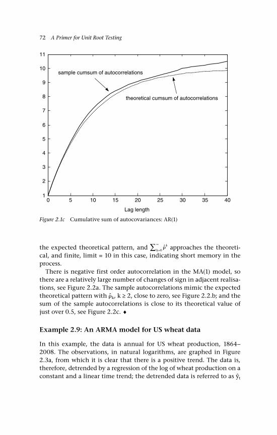
72 A Primer for Unit Root Testing
the expected theoretical pattern, and k
k=
∞∑ 0 approaches the theoreti-cal, and finite, limit = 10 in this case, indicating short memory in the process.
There is negative first order autocorrelation in the MA(1) model, so there are a relatively large number of changes of sign in adjacent realisa-tions, see Figure 2.2a. The sample autocorrelations mimic the expected theoretical pattern with k, k ≥ 2, close to zero, see Figure 2.2.b; and the sum of the sample autocorrelations is close to its theoretical value of just over 0.5, see Figure 2.2c. ♦
Example 2.9: An ARMA model for US wheat data
In this example, the data is annual for US wheat production, 1864–2008. The observations, in natural logarithms, are graphed in Figure 2.3a, from which it is clear that there is a positive trend. The data is, therefore, detrended by a regression of the log of wheat production on a constant and a linear time trend; the detrended data is referred to as yt
0 5 10 15 20 25 30 35 401
2
3
4
5
6
7
8
9
10
11
theoretical cumsum of autocorrelations
sample cumsum of autocorrelations
Lag length
Figure 2.1c Cumulative sum of autocovariances: AR(1)
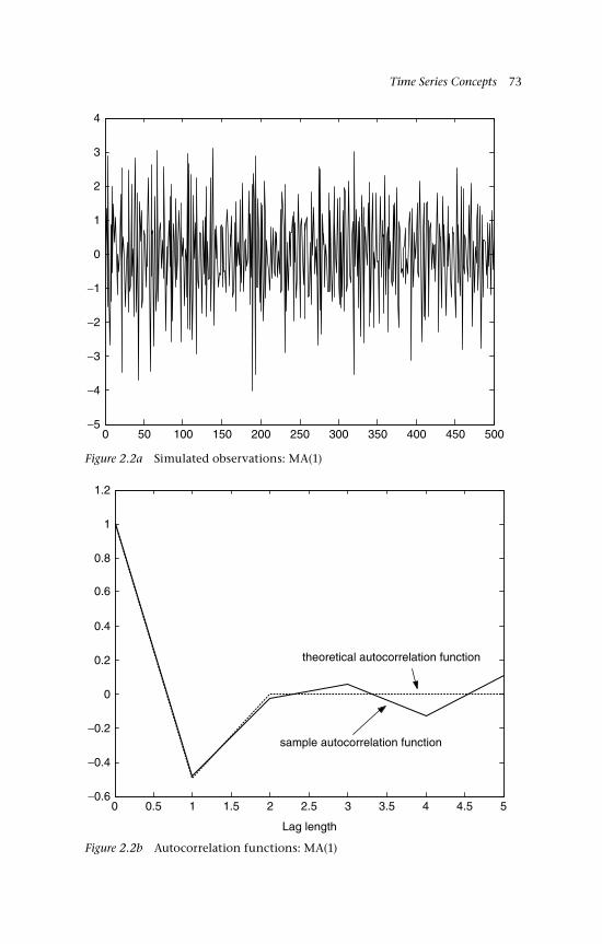
Time Series Concepts 73
Figure 2.2a Simulated observations: MA(1)
0 50 100 150 200 250 300 350 400 450 500−5
−4
−3
−2
−1
0
1
2
3
4
Figure 2.2b Autocorrelation functions: MA(1)
0 0.5 1 1.5 2 2.5 3 3.5 4 4.5 5−0.6
−0.4
−0.2
0
0.2
0.4
0.6
0.8
1
1.2
sample autocorrelation function
Lag length
theoretical autocorrelation function
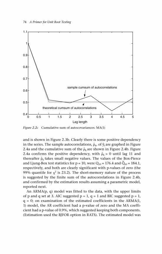
74 A Primer for Unit Root Testing
and is shown in Figure 2.3b. Clearly there is some positive dependency in the series. The sample autocorrelations, k, of yt are graphed in Figure 2.4a and the cumulative sum of the k are shown in Figure 2.4b. Figure 2.4a confirms the positive dependency, with k > 0 until lag 11 and thereafter k takes small negative values. The values of the Box-Pierce and Ljung-Box test statistics for p = 10, were Q10 = 176.4 and Q10 = 184.1, respectively, and both are clearly significant with p-values of zero (the 99% quantile for 2 is 23.2). The short-memory nature of the process is suggested by the finite sum of the autocorrelations in Figure 2.4b, and confirmed by the estimation results assuming a parametric model, reported next.
An ARMA(p, q) model was fitted to the data, with the upper limits of p and q set at 3. AIC suggested p = 1, q = 1 and BIC suggested p = 1, q = 0; on examination of the estimated coefficients in the ARMA(1, 1) model, the AR coefficient had a p-value of zero and the MA coeffi-cient had a p-value of 0.9%, which suggested keeping both components. (Estimation used the BJFOR option in RATS). The estimated model was
Figure 2.2c Cumulative sum of autocovariances: MA(1)
0 0.5 1 1.5 2 2.5 3 3.5 4 4.5 50.4
0.5
0.6
0.7
0.8
0.9
1
1.1
sample cumsum of autocorrelations
theoretical cumsum of autocorrelations
Lag length

Time Series Concepts 75
Figure 2.3a US wheat production (log)
1880 1900 1920 1940 1960 1980 200012
12.5
13
13.5
14
14.5
15
Figure 2.3b US wheat production (log, detrended)
1880 1900 1920 1940 1960 1980 2000−0.8
−0.6
−0.4
−0.2
0
0.2
0.4
0.6
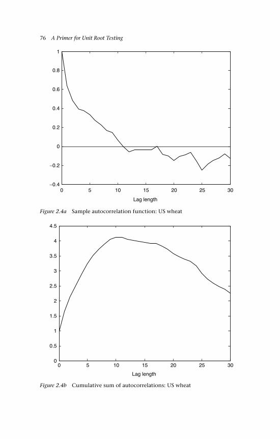
76 A Primer for Unit Root Testing
Figure 2.4a Sample autocorrelation function: US wheat
Figure 2.4b Cumulative sum of autocorrelations: US wheat
0 5 10 15 20 25 30−0.4
−0.2
0
0.2
0.4
0.6
0.8
1
Lag length
0 5 10 15 20 25 300
0.5
1
1.5
2
2.5
3
3.5
4
4.5
Lag length
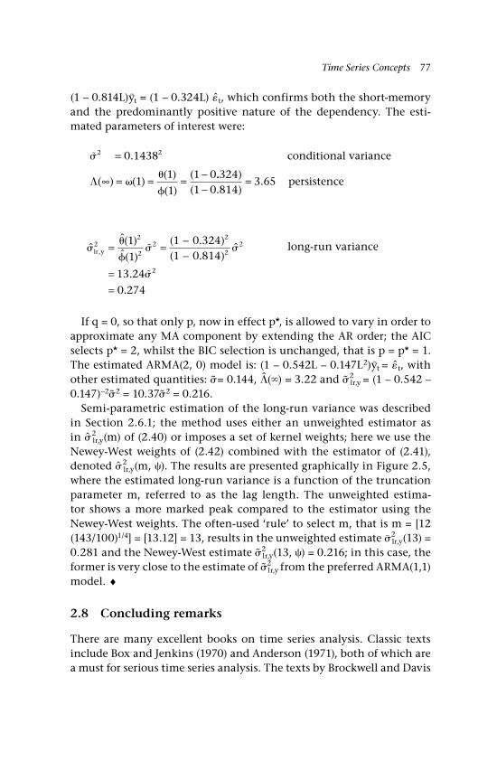
Time Series Concepts 77
(1 – 0.814L)y~t = (1 – 0.324L) t, which confirms both the short-memory and the predominantly positive nature of the dependency. The esti-mated parameters of interest were:
2 20 1438
11
1
1 0
=
∞ = = = −
.
( ) ( )( )
( )
(
conditional variance
.. )
( . ).
3241 0 814
3 65−
= persistence
ˆ( )
ˆ( )
( . )( . )
ˆ
.
,
lr y2
2
22
2
22
2
1
1
1 0 3241 0 814
13 24
0
= =−−
== ..274
long-run variance
If q = 0, so that only p, now in effect p*, is allowed to vary in order to approximate any MA component by extending the AR order; the AIC selects p* = 2, whilst the BIC selection is unchanged, that is p = p* = 1. The estimated ARMA(2, 0) model is: (1 – 0.542L – 0.147L2)y~t = t, with other estimated quantities: = 0.144, () = 3.22 and
2lr,y = (1 – 0.542 –
0.147)–2 2 = 10.37
2 = 0.216.Semi-parametric estimation of the long-run variance was described
in Section 2.6.1; the method uses either an unweighted estimator as in 2
lr,y(m) of (2.40) or imposes a set of kernel weights; here we use the Newey-West weights of (2.42) combined with the estimator of (2.41), denoted 2
lr,y(m, ). The results are presented graphically in Figure 2.5, where the estimated long-run variance is a function of the truncation parameter m, referred to as the lag length. The unweighted estima-tor shows a more marked peak compared to the estimator using the Newey-West weights. The often-used ‘rule’ to select m, that is m = [12 (143/100)1/4] = [13.12] = 13, results in the unweighted estimate ∼
2lr,y(13) =
0.281 and the Newey-West estimate 2lr,y(13, ) = 0.216; in this case, the
former is very close to the estimate of 2lr,y from the preferred ARMA(1,1)
model. ♦
2.8 Concluding remarks
There are many excellent books on time series analysis. Classic texts include Box and Jenkins (1970) and Anderson (1971), both of which are a must for serious time series analysis. The texts by Brockwell and Davis
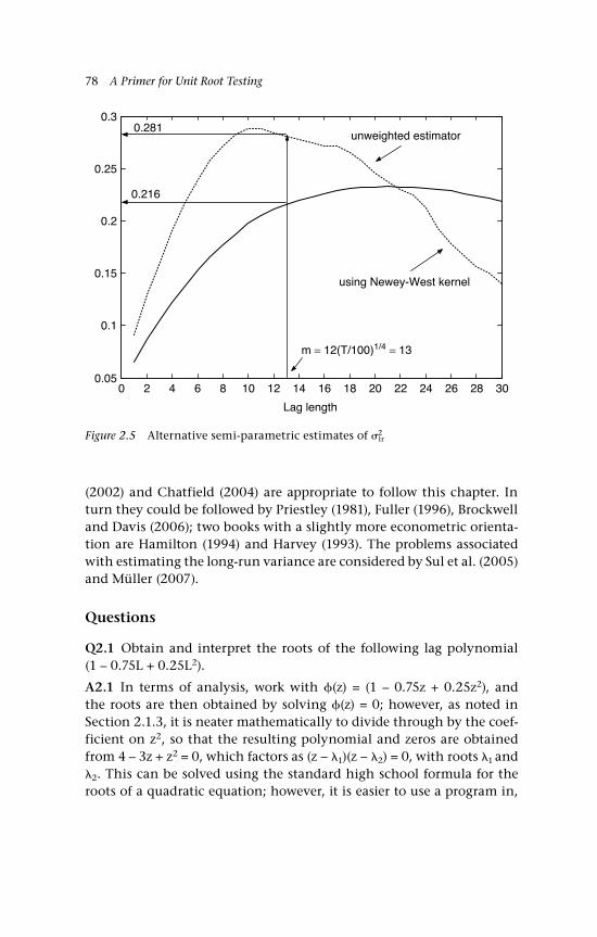
78 A Primer for Unit Root Testing
(2002) and Chatfield (2004) are appropriate to follow this chapter. In turn they could be followed by Priestley (1981), Fuller (1996), Brockwell and Davis (2006); two books with a slightly more econometric orienta-tion are Hamilton (1994) and Harvey (1993). The problems associated with estimating the long-run variance are considered by Sul et al. (2005) and Müller (2007).
Questions
Q2.1 Obtain and interpret the roots of the following lag polynomial (1 – 0.75L + 0.25L2).
A2.1 In terms of analysis, work with (z) = (1 – 0.75z + 0.25z2), and the roots are then obtained by solving (z) = 0; however, as noted in Section 2.1.3, it is neater mathematically to divide through by the coef-ficient on z2, so that the resulting polynomial and zeros are obtained from 4 – 3z + z2 = 0, which factors as (z − 1)(z − 2) = 0, with roots 1 and 2. This can be solved using the standard high school formula for the roots of a quadratic equation; however, it is easier to use a program in,
0 2 4 6 8 10 12 14 16 18 20 22 24 26 28 300.05
0.1
0.15
0.2
0.25
0.3
Lag length
unweighted estimator
using Newey-West kernel
0.216
0.281
m = 12(T/100)1/4 = 13
Figure 2.5 Alternative semi-parametric estimates of 2lr
Time Series Concepts 79
for example MATLAB, as used here, to obtain the roots. The MATLAB instructions are:
p = [1 −3 4]r = roots(p)absr = abs(r)
Note that the polynomial coefficients are typed in declining order of the powers in the polynomial; thus the coefficient on z2 is read in first, and the constant is last. (Note that the same results are obtained provided that the ratio of the coefficients is maintained, so that p = [1/4 –3/4 1], gives the same results, see Q2.3 below.) The output is:
p = [1 −3 4]r = 1.5000 + 1.3229i 1.5000 − 1.3229iabsr = 2 2
In the notation of this chapter, the roots are: 1, 2 = 1.5 ± 1.323i, which is a pair of conjugate complex numbers, with the same modu-lus given by | 1 |, | 2 | = ( . . )1 5 1 323 22 2+ = . The modulus of the roots is greater than 1 and the roots are said to be ‘outside the unit cir-cle’, so that the AR(2) model constructed from this lag polynomial is invertible.
To check that 1 and 2 are indeed the roots, the polynomial (z − 1) (z − 2) is reconstructed using the numerical values of 1 and 2. The MATLAB instructions and output are as follows:
pp = poly(r)pp = 1 −3 4
Q2.2 Confirm the result used in example 2.7, that:
ACGF zz z
z z z z
( )( )( )
( ( ) ) ( ( ) (
=− −
= + + + + + + +
−
−
11 1
1 1
12
2 2 2 1 2
−− +( )2 2)
80 A Primer for Unit Root Testing
A2.2 The first part of the answer uses the result for convergent series that:
11 0( )−
==
∞∑
z
zj j
j
Also replace z by z–1 to obtain an analogous result for (1 – z–1)–1. Now write out some illustrative terms:
(1 1
1
2 2 3 3 1 2 2 3 3
2 2 3
+ + + +( ) + + + +( )+ + + +
=
− − −
z z z z z z
z z z
zz z
z z
−
− −
+ + +
+ +
1 2 3
2 2 3 1
The trick is to pick off the coefficients on powers of z. For example, the coefficients on z0 1, z, z2 and the general term, zk, are, respectively:
( ) ( )
( ) ( )
(
1 1
1 1
1
2 4 6 2 1
2 4 6 2 1
2 2 4
+ + + + = −
+ + + + = −
+ +
−
−
++ + = −
+ + + + = −
−
−
6 2 2 1
2 4 6 2 1
1
1 1
) ( )
( ) ( )k k
Multiplying the general term by 2 gives the k-th order autocovariance.
Q2.3 Compare the AR and MA roots of the following ARM(p, q) mod-els, based on an example from Chapter 8, which uses the log ratio of the fold to silver prices. The first model is the ARMA(2, 1) given by:
(1 + 0.940L + 0.130L2) y~t = (1 + 0.788L)t, = 0.0137
The second model is the following ARMA(1, 0) model (estimated on the same data set):
(1 + 0.152L) y~t = t, = 0.0137.
Why is the estimate of from the two models, indistinguishable?

Time Series Concepts 81
A2.3. In the first case, the roots of the AR(2) polynomial (1 + 0.940z + 0.130z2) can be obtained from MATLAB as follows:
p = [0.13 0.94 1]r = roots(p) = −1.2962, −5.9346
The reciprocals of the roots are obtained as:
rr = 1./r = –0.7715, –0.1685
Hence, the polynomial can be factored as:
(1 + 0.940z + 0.130z2) = (1 + 0.7715z) (1 + 0.1685z)
If you were tempted to obtain the measure of long-run persistence using this polynomial, the following would result:
ˆ( )( . )
( . )( ..
∞ = ++ +
=
1 0 7881 0 7715 1 0 1
0 864
However, note that the reciprocal of the first root, that is 0.7715, is very close to the MA(1) coefficient of 0.788, so that there is a near cancella-tion of roots in the AR and MA polynomials, that is:
( . )( . )( . ) ( . )
1 0 7881 0 7715 1 0 1685
11 0 1685
++ +
≈+
LL L L
Thus, moving to the ARMA(1, 0) model, the root of the AR(1) polyno-mial is
p = [0.152 1]r = roots(p) = −6.5789
As expected, this single root is close to one of the roots of the AR(2) polynomial, confirming the suspicion of a common factor. Finally, note that the persistence measure based on the AR(1, 0) model is cal-culated as:
ˆ( )( . ).
∞ =+
=
11 0 152
0 868
82 A Primer for Unit Root Testing
Which differs only slightly from the over-parameterised ARM(2, 1) model. In effect, the ARMA(2, 1) model has nothing to add over the ARMA(!, 0) model, hence their estimated standard errors and associated statistics differ only marginally.
The estimator of the long-run variance for the preferred model is then given as follows:
ˆ
.
ˆ .
lr,y2 2
lr,y2
0.868 (0.0137)= ×
=
=
0 000141
0 0119
Q2.4.i Let yt = yt–1 + ut and u = (u1, ..., uT). Show that the long-run variance 2
lr,u of ut is the limiting sum of all of the elements in the cov-ariance matrix of u; hence, derive 2
lr,u = j=– j. Note that this set-up
is the most familiar form in which the long-run variance is required; for example, it is important in the functional central limit theorem of Chapter 6; and a unit root test will generally not be valid unless an adjustment is made for 2
lr,u ≠ 2 , see Chapter 8.
Q2.4.ii Show that S2T,u may be equivalently expressed as:
S u
u u u
T u tt
T
tt
T
t t kt k
T
k
T
,2
1
2
2
1 11
12
= ( )= +
=
= −= +=
−
∑∑ ∑∑
Note that this is an often used form for S2T,u, as shown in Section 2.6.1
on estimating the long-run variance by semi-parametric methods; in that section, the notational set-up was for y~t rather than ut.
A2.4.i Consider the partial sum process constructed from ut, St = tj=1 uj
and the long-run variance 2lr,u of ut. Then we have, by definition:
lr u T TT E S, lim ( )2 1 2≡ →∞−
Next write ST = iu, where i = (1, ..., 1) and u = (u1, ..., uT) and, therefore:
E S E u uT( ) ( ’ )( ’ )2 = i i
= E[iu(ui)] because iu is a scalar and, therefore, iu = ui = iE(uu)i
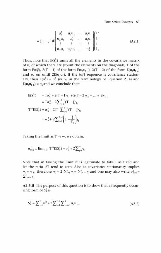
Time Series Concepts 83
=
( , , )1 1
12
1 2 1
2 1 22
1
1 22
E
u u u u u
u u u u u
u u u u u
T
T
T T T
1
1
1
(A2.1)
Thus, note that E(ST2 ) sums all the elements in the covariance matrix
of u, of which there are (count the elements on the diagonals) T of the form E(ut
2), 2(T − 1) of the form E(utut–1), 2(T − 2) of the form E(utut–2) and so on until 2E(u1uT). If the ut
2 sequence is covariance station-ary, then E(ut
2) = u2 (or 0 in the terminology of Equation 2.14) and
E(utut–k) = k and we conclude that:
E S T T T
T T j
T u T
u j
T
j
( ) ( ) ( )
( )
2 21 2 1
2
1
1
2 1 2 2 2
2
= + − + − + +
= + −−
=
−∑
TT E S T T j
jT
T u j
T
j
uT
j
T
− −=
−
=
−
= + −
= + −
∑
∑
1 2 2 1
1
1
2
1
1
2
2 1
( ) ( )
jj
Taking the limit as T → ∞, we obtain:
lr u T T u jjT E S, lim ( )2 1 2 2
12≡ = +→∞
−=
∞∑
Note that in taking the limit it is legitimate to take j as fixed and let the ratio j/T tend to zero. Also as covariance stationarity implies k = –k, therefore 0 + 2
j=1 j = j=– j and one may also write 2
lr,u =
j=– j.
A2.5.ii The purpose of this question is to show that a frequently occur-ring form of S2
T is:
S u u uT tt
T
t t kt k
T
k
T2 2
1 11
12= +
= −= +=
−∑ ∑∑ (A2.2)
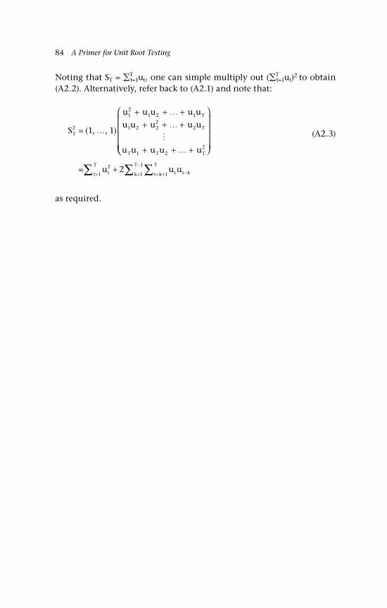
84 A Primer for Unit Root Testing
Noting that ST = Tt=1ut, one can simple multiply out (T
t=1ut)2 to obtain
(A2.2). Alternatively, refer back to (A2.1) and note that:
S
u u u u u
u u u u u
u u u u u
T
T
T
T T T
2
12
1 2 1
1 2 22
2
1 22
1 1=
+ + ++ + +
+ + +
( , , )
(A2.3)
= u u utt
T
t t kt k
T
k
T2
1 11
12
= −= +=
−∑ ∑∑+
as required.

3Dependence and Related Concepts
85
This chapter introduces a number of concepts and models that have in common the central concern of characterising the dependence in a stochastic process. Intuitively we are interested in whether what hap-pens at time t has been affected by what happened before that time, sometimes referred to the ‘memory’ of the process. In an economic context, the more usual situation is that stochastic processes have memory to some degree and our interest is in assessing the extent of that memory. This is important for the generalisation of the central limit theorem (CLT), see Chapter 4, Section 4.2.3, and the functional CLT, see Chapter 6, Section 6.6.1.
This chapter is organised as follows. The concept of temporal depend-ence is introduced in Section 3.1; and the generalisation of weak sta-tionarity to asymptotic weak stationarity, which is particularly relevant for processes with an AR component, is considered in Section 3.2; ergodicity, and particularly ergodicity in the mean are considered in Section 3.3; Section 3.4 collects some results for ARMA models; Section 3.5 introduces two properties of particular interest in economics and finance, which serve to define a martingale sequence and a Markov process, respectively.
3.1 Temporal dependence
The idea of temporal dependence was introduced in Chapter 2; it is, for example, implicit in the concept of persistence and explicit in the auto-covariances and long-run variance. In the case of persistence, the impact of a shock is captured by (L) and (1), the coefficients and sum of the coef-ficients in the MA representation of an ARMA process. One characterisa-tion of a process without dependence is j = 0, j = 1, ... ∞ ⇒ (1) = 1; this is
86 A Primer for Unit Root Testing
a limiting and rather uninteresting case, but serves to contrast with other cases for which j ≠ 0 for some j ! 1 and (1) ≠ 1. An important way of assessing dependence is through the autocovariances, which is the sub-ject of the next section.
3.1.1 Weak dependence
Reference was made in Chapter 2 to the summability of the autocovari-ance and autocorrelation sequences for an AR(1) DGP. If | | < 1, then the process exhibits temporal dependence, but it is weak enough that the links between elements in the sequence yt are ‘forgotten’ for elements sufficiently far apart. This is indicated by the k-th autocovariance, k, tending to zero sufficiently fast as k → ∞, such that lim | |K kk
K
→∞ =∑ 0
= c, a finite constant. This is a condition referred to as absolute summability of the autocovariances; it is usually taken to define a ‘short-memory’ process. In the case of the AR(1) model, if → 1 then lim | |K kk
K
→∞ =∑ 0
→ ∞, and this is a particular form of ‘long memory’. If the autocovariances are absolutely summable, then the sequence yt is said to be weakly dependent. Also note that absolute summability implies kk
2
0=
∞∑ < ∞, but not vice-versa (Section 3.4 below for a summary of relevant results).
3.1.2 Strong mixing
As a preliminary to the formality of the condition of strong mixing, consider the straightforward definition of independence given in Chapter 1, Equation (1.4), as it is applied to yt and yt shifted by s peri-ods, that is yt+s. In that case yt and yt+s are independent and dependent, respectively, if:
P y y P y P yt t s t t s( ) ( ) ( )∩ − =+ + 0 (3.1a)
P y y P y P yt t s t t s( ) ( ) ( )∩ − ≠+ + 0 (3.1b)
In the latter situation an interesting case to consider is where the extent of the dependence is limited, so that it tends to zero as s → ∞, that is for s ‘sufficiently’ far from t. Thus, the sequence yt may well exhibit short range dependence, but of a form that, in a well-defined sense, becomes less important over time. To this effect, dependence is limited if:
| ( ) ( ) ( ) |
| ( ) ( ) ( ) |
P y y P y P y
P y y P y P y
t t t t
t t s t t s
∩ − < < ∞
∩ − <
+ +
+ +
1 1 1
s < ∞
Dependence and Related Concepts 87
with the condition that s → 0 as s → ∞. This is an example of a more general concept known as strong mixing, which is a way of characteris-ing the extent of dependence in the sequence of yt. It was introduced by Rosenblatt (1956) and is one of a number of mixing conditions; for a sur-vey see Bradley (2005), who considers eight measures of dependence.
Strong mixing is put into a more formal context as follows. Consider the sequence of random variables Y = yt
and let Ftt+s be the –field
generated by the subset sequence yj j tt s=+ , s ≥ 0. (The process could be
started at t = 0, without altering the substance of this section.) Ftt+s is
the –field generated by a particular time series ‘portion’ of yt over the period t to t + s, s ≥ 0; for example, (yt) for s = 0, (yt, yt+1) for s = 1 and so on. Further, (yt+s, ..., y) is the –field generated by the ran-dom variables from yt+s onward and (y–, ..., yt) is the –field generated by random variables from the start of the process to time t. As we are here dealing with essentially time-ordered sequences, the fields Ft
t+s are inclusive or nested, such that Ft
t+s Ftt+s+1 Ft
t+s+2 and so on, known as increasing sub-algebras; this feature of Ft
t+s is a property that is relevant for martingale sequences, see Section 3.5.1 below.
Let A denote a set in F–t and B a set in F
t+s, so the sequences of compar-ison comprise, respectively, the –field generated by the random vari-ables in the two time series ‘portions’ yjtj=– and yj
j=t+s. Next define the mixing coefficients s by:
sup sup | ( ) ( ) ( ) |,t A F B Ft
t sp A B p A p B
∈ ∈−∞ +∞ ∩ −( )( ) ≡ s
(3.2)
The sequence jsj=1 is a sequence of ‘mixing’ coefficients. If s 0 as s →
∞, then yt is said to be strong mixing, usually referred to as -mixing.The notation ‘sup’ applied to a set with elements that are real num-
bers means the supremum or least upper bound: it is the least (small-est) real number that is greater than or equal to every element (real number) in the set. For example, let the set A(), with elements ai, be such that A() = (ai : – < c < ai < b < ), then supi A() = b; note that b is not actually in A() as defined, so it differs from the maximum value (‘max’), although if the sup is in the set, then it is the maximum element.
In the definition of strong mixing, the first ‘sup’ to consider is the inner one, which looks for the least upper bound across all elements of the sets A and B for fixed t; the second sup then just allows t to vary. The idea is that a sequence is strong mixing or -mixing, if the (maximum)
88 A Primer for Unit Root Testing
dependence as indexed by s dies out for s, the time separation indica-tor, sufficiently large; thus, independence is achieved asymptotically.
Stationary MA(1) and AR(1) processes are generally -mixing as are more general stationary ARMA(p, q) processes; the ‘generally’ implies that there are some exceptions. One such was highlighted by Andrews (1983), who showed that an AR(1) process, with (0, ½], and stochas-tic inputs t, including 0, generated as Bernouilli random variables, is not strong mixing. What is required additionally is that the distribu-tion of the random variable 0 is smooth. The formal condition is stated in Andrews (1983, especially Theorem 1), and is satisfied by a large number of distributions including the normal, exponential, uniform and Cauchy (which has no moments).
The importance of the concept of strong mixing is two-fold in the present context. First, in the context of the (standard) central limit the-orem, CLT, see Chapter 4, Section 4.2.3, an interesting question is how much dependence is allowed in the sequence of stochastic inputs, such that the CLT still holds. The CLT can be regarded as providing an ‘invar-iance’ principle, in the sense it holds for a broad set of specifications of the marginal and joint distributions of the stochastic inputs. However, notwithstanding its importance elsewhere, what is more important in context is the extension of the CLT to the functional CLT, see Chapter 6, Section 6.6.1, which again provides an invariance principle, but this time one that is relevant to unit root testing.
3.2 Asymptotic weak stationarity
The concept of stationarity, in the forms of strict and weak or covari-ance stationarity, was introduced in Chapter 1, Section 1.9. A slight vari-ation on weak stationarity (WS), which is particularly relevant for AR models, is asymptotic weak stationarity. The idea is that the process is nonstationary for a finite sample size, T, but becomes stationary as T ∞. An example will illustrate the point.
Example 3.1: AR(1) model
Consider the stochastic process generated by the AR(1) model:
y yt t t= +− 1 (3.7)
where t is a white noise input. Adopt the convention that y0 (rather than y–) is the starting value, where y0 is a bounded random variable
Dependence and Related Concepts 89
with E(y0) = 0 and var(y0) < ∞. By repeated (back)substitution using (3.7), the solution in terms of the initial condition and intervening shocks is:
y ytt i
t ii
t= + −=∑ 0 1 (3.8)
The variance of yt is given by:
var( ) var
var( ) var
y y
y
tt i
t ii
t
t it ii
t
= +( )= +
−=
−
−=
−
∑
0 0
1
20 0
1∑∑∑
( )= +
= +
−=
−
=
20
2
0
1
20
2 2
0
t it ii
t
t i
i
t
y
y
var( ) var( )
var( ) ( )−−∑ 1
(3.9)
Notice that neither term in the variance is constant as t varies, both having the feature that the dependence declines as t increases for given | | < 1. The second term can be expressed as:
2 2
1
2
22
2
21 1( )
( ) ( )i
i
t t
=∑ =−
−−
(3.10)
Hence, as t → ∞, for | | < 1, only the first term survives. This means that for an arbitrary var(y0) < ∞ (for example, var(y0) = 0 if y0 is a constant), then var(yt) is not constant, but it converges to a constant.
Alternatively, note that setting var(y0) = 2(1 – 2)–1, which is an option in a Monte-Carlo setting to generate the data, is equivalent to starting the process in the infinite past; then 2t var(y0) = 2t2(1 – 2)–1, so that var(yt) = 2(1 – 2)–1, which is a constant. This assumption is often pre-ferred for var(y0) as it generates a weakly stationary process. ♦
3.3 Ensemble averaging and ergodicity
The problem we are usually faced with in practice is an inability to replicate the data generation process, DGP, to produce repeated sam-ples. We observe one particular set of realisations, or sample outcomes, and the question is what can we infer from this one set? For example, suppose we would like to know the means of the variables yt, E(yt), t = 1, ... , T, each of which is a (discrete) random variable with N possible
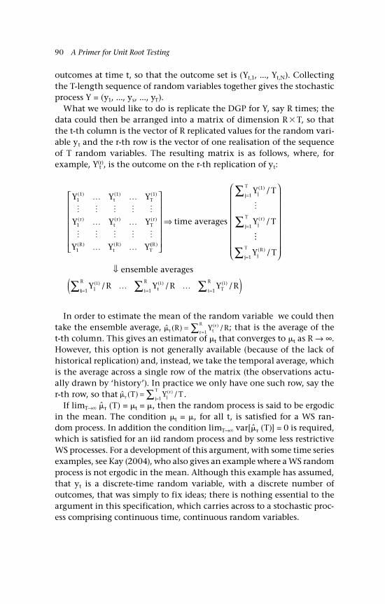
90 A Primer for Unit Root Testing
outcomes at time t, so that the outcome set is (Yt,1, ..., Yt,N). Collecting the T-length sequence of random variables together gives the stochastic process Y = (y1, ..., ys, ..., yT).
What we would like to do is replicate the DGP for Y, say R times; the data could then be arranged into a matrix of dimension R T, so that the t-th column is the vector of R replicated values for the random vari-able yt and the r-th row is the vector of one realisation of the sequence of T random variables. The resulting matrix is as follows, where, for example, Y(r)
t , is the outcome on the r-th replication of yt:
Y Y Y
Y Y Y
Y Y Y
t T
rt
rT
r
Rt
RT
11 1 1
1
1
( ) ( ) ( )
( ) ( ) ( )
( ) ( ) (( )
( )
( )
/
/
R
jj
T
jr
j
Ttime averages
Y T
Y T
⇒
=
=
∑
∑
1
1
1
Y T
ensemble averages
Y R
jR
j
T
i
( )
( )
/
/
=∑
⇓1
1ii
R
ti
i
R
Ti
i
RY R Y R
= = =∑ ∑ ∑( )1 1 1
( ) ( )/ /
In order to estimate the mean of the random variable we could then take the ensemble average, ˆ ( ) /( )t t
r
r
RR Y R=
=∑ 1; that is the average of the
t-th column. This gives an estimator of t that converges to t as R → ∞. However, this option is not generally available (because of the lack of historical replication) and, instead, we take the temporal average, which is the average across a single row of the matrix (the observations actu-ally drawn by ‘history’). In practice we only have one such row, say the r-th row, so that ˆ ( ) /( )r j
r
j
TT Y T=
=∑ 1.
If limT→ r (T) = t = , then the random process is said to be ergodic in the mean. The condition t = , for all t, is satisfied for a WS ran-dom process. In addition the condition limT→ var[r (T)] = 0 is required, which is satisfied for an iid random process and by some less restrictive WS processes. For a development of this argument, with some time series examples, see Kay (2004), who also gives an example where a WS random process is not ergodic in the mean. Although this example has assumed, that yt is a discrete-time random variable, with a discrete number of outcomes, that was simply to fix ideas; there is nothing essential to the argument in this specification, which carries across to a stochastic proc-ess comprising continuous time, continuous random variables.
Dependence and Related Concepts 91
3.4 Some results for ARMA models
In this section we gather together some useful results (without proof), connected to dependence, and relate them to ARMA processes. In part this just collects together previous results for convenience.
Let be kk=0 a sequence of constants, then the sequence is said to be
absolutely summable if k=0 | k | < ∞. If k = –, ... , , the definition of
absolute summability is altered accordingly through a change in the lower limit. The sequence is said to be square summable if
k=0 | 2k | < ∞.
Absolute summability implies square summability, but not vice-versa:
| | kk k< ∞ ⇒ < ∞
=
∞
=
∞∑ ∑0 0 k2
If the sequence of autocovariances of yt is absolutely summable, then yt is said to be weakly dependent; that is, a process with weak depend-ence or, equivalently, short memory, necessarily has the property
k=0 | k | < ∞.
Next suppose that yt is generated by a causal ARMA(p, q) process, with MA representation (see Chapter 2, Equation (2.7)) given by:
yt jj t j==
∞−∑
0«
Then, in terms of the MA coefficients and autocovariance coeffi-cients, we have:
1. | | kk kk=
∞
=
∞∑ ∑< ∞ ⇒ < ∞0
2
0
2. | | kk kk=
∞
=
∞∑ ∑< ∞ ⇒ < ∞0
2
0
3. | | kk kk=
∞
=
∞∑ ∑< ∞ ⇒ < ∞0
2
0
4. | | | | kk kk=
∞
=
∞∑ ∑< ∞ ⇒ < ∞0 0
5. kk ty2
0< ∞ ⇒
=
∞∑ is covariance stationary
6. | |kk ty=
∞∑ < ∞ ⇒0 is ergodic for the mean and covariance (weakly)
stationary by 1 and 5.
3.5 Some important processes
This section introduces two properties that are relevant to stochastic processes that have a particular role in subsequent chapters. The first is the martingale, which is central to financial econometrics, especially its role in the Itô calculus (see Chapters 6 and 7), and to unit root testing
92 A Primer for Unit Root Testing
through its role as a prototypical time series process. (Some of the nec-essary background has already been undertaken in Section 3.1.2.) The second property results is that of a Markov process which, although less significant in the present development, characterises an important feature of some economic time series.
3.5.1 A Martingale
Consider the stochastic process Y = (yt, 0 t < ) and let the sequence of –fields H = (Ht
0, 0 t < ) represent ‘history’ to time t, not neces-sarily just the history of Y. Given the gambling context in which the concept of a martingale arose, the stochastic process is assumed to start at a particular finite point of history, rather than in the infinite past. (The time index assumes that time is discrete and t ", but the argu-ments carry across to t and to the continuous-time case replacing yt by y(t) and so on.)
On the assumption that history is not lost, then Hs0 Ht
0 for s < t, and H is a nested sequence, referred to as a filtration. Y is said to be adapted to the filtration H if (ys, ..., y0) Hs
0 for all s ≤ t. The natural filtration is the sequence of –fields associated with Y, that is F = (Ft
0 , 0 t < ) where Ft
0 = (yt, yt–1, ...). Y is adapted to the natural filtration as (ys, ..., y0) Fs
0 . In an economic context, the filtrations can be thought of as information sets and usually no violence is done to the meaning to sub-stitute the information set, say (yt, yt–1, ..., y0), for Ft
0 ; although theoreti-cally, conditional expectations are more soundly based when viewed as being based on –fields, rather than information sets, see, for example, Davidson (1994) and Shreve (2004).
A martingale stochastic process is defined with respect to a filtration (or information set). Here we take that filtration to be F, although the definition allows other filtrations (for example H). Y is a martingale with respect to the filtration F if:
i. E| yt | < ∞ ii. Y is adapted to Fiii. E[yt | Fs
0] = ys for all s < t
As the –field Fs0 can be generated from (ys, ys–1, ...) the last condition, in
a form that is more familiar (in an economic sense of forming expecta-tions), is:
E y y y yt s s s[ | , , ]− =1 for all s < t (3.11)

Dependence and Related Concepts 93
For example, if s = t – 1, then the martingale property is:
E y y y yt t t t[ | , , ]− − −=1 2 1 (3.12)
For emphasis one might also date the expectation, say Et–1 for an expec-tation formed at time t – 1, thus (3.12) is Et–1[yt | yt–1, yt–2, ...] = yt–1, but the general understanding is that the date of the formation of the conditional expectation matches the most recent date in the informa-tion set. For example, suppose that yt is the price of a financial asset, then by taking the expectation one period forward (say ‘tomorrow’), the expected value of tomorrow’s price is the price today: E[yt+1 | yt, yt–1, ..., y0] = yt , where the expectation is implicitly dated at t.
Note that E(yt | yt, yt–1, ...) = E(yt) = yt, as yt is included in the filtra-tion and so has happened at the time of the information set. Thus, an implication of the martingale condition is that:
E y y y yt t t t[( ) | , , ]+ −− =1 1 0 (3.13)
An interpretation of this condition is that viewed as a game, the process generating yt is said to be fair. No systematic gains or losses will be made if the game is replicated. If yt is an asset price, and the conditioning set is current information, then the change in price is unpredictable in the mean.
As yt+1 yt+1 – yt, then to focus on the differences (3.13) can be writ-ten in general terms as:
E y y yt t t[ | , ,...] + − =1 1 0 (3.14)
A sequence of differences with this property is referred to as a martin-gale difference sequence or MDS. An MDS has serially uncorrelated, but not necessarily independent, stochastic increments. Neither does a MDS require that the variance or higher order moments are constant. A leading example is where the squared levels depend upon past values of yt, as in an ARCH or GARCH model, so that E(y2
t | yt–1, yt–2, ..., y0) = f(F0t–1)
and the variance is predictable from F0t–1.
Example 3.2: Partial sum process with −1/+1 inputs
Consider a random variable yt with two outcomes taking the value –1 with probability p and the value +1 with probability 1 – p, so that E(yt) = –1 p + (+1) (1 – p) = (1 – 2p). Let St = t
j=1yj and the random process

94 A Primer for Unit Root Testing
comprise the sequence of St, where yt is stochastically independent of ys for t ≠ s. Then St = St–1 + yt, which is an asymmetric random walk, but not a martingale unless p = ½, as in the coin-tossing game with a fair coin. First, observe that when p ≠ ½, yt is not a fair game. The sequence of unconditional expectations is: E(S1) = 1 – 2p, E(S2) = 2(1 – 2p) and so on, with general term E(St) = t(1 – 2p); for example if p = ¼, then the expected loss on the game at t = 10 is 5. Consider the conditional expec-tation (3.13) applied in this case:
E S S y y y
E S S y
E y y
E
t t t t t
t t t t
t t t
t
[( ) | , , , ]
[( ) | ]
[ | ]
+ −
+
+
−
= −
=
=
1 1 0
1
1
(( )
( )
y
pt+
= −1
1 2 (3.15)
The second last equality follows from the assumption of stochastic independence. Note that (1 – 2p) ≠ 0 unless p = ½, so that generally the game is not fair and not a martingale. However, a martingale can be constructed from yt by making the game fair; that is, by removing the non-zero mean, and to this effect define the random process con-structed from the random variables zt = St – t(1 – 2p). Then to assess the fairness of the game consider Et[zt+1 | zt] where zt+1 = St+1 – ∆(t + 1)(1 – 2p) = yt+1 – (1 – 2p); hence, E[yt+1 – (1 – 2p) | zt] = (1 – 2p) – (1 – 2p) = 0, on substituting from (3.15), and the game is fair. ♦
Example 3.3: A psp with martingale inputs
Consider the partial sum process (psp) of example 1.9, so that S yt jj
t=
=∑ 1
and Y = (y1, y2, ..., yt), but assume directly that Y is a martingale with respect to the natural filtration, then E S E yt jj
t( ) ( )2 2
1=
=∑ , a result that had previously been associated with yj being iid(0, 2). See question Q3.3 for an outline of the proof. The impact of this property is that it enables a generalisation of some important theorems in statistics and econometrics to other than iid sequences; for example, the cen-tral limit theorem and the weak law of large numbers see Chapter 4, Section 4.2.7. ♦
3.5.2 Markov process
The Markov property characterises the memory of a stochastic process. Consider the stochastic process Y = (yt, 0 t < ), then the Markov

Dependence and Related Concepts 95
property is:
P y A y y y P y A yt h t s t t h t s( | , ,..., ) ( | )+ − − + −∈ = ∈2 0 (3.16)
for all h ≥ 0, s ≥ 0 and A . First note that time is of the essence in defining the Markov property. In the language of Markov chains, yt is the ‘state’ at time t and the set A is specialised to a particular state, say yt = y. The Markov property is then often stated for the case h = 0 and s = 1, so that:
P y y y y y P y y yt t t t t( | , ,..., ) ( | )= = =− − −1 2 0 1 (3.17)
Thus, information prior to t – 1 has no influence on the probability that yt is in state y; there is no memory concerning that part of the informa-tion set. Given this property it should not be a surprise that moving the index h forward leads to the same conclusion:
P y y y y y P y y yt t t t t( | , ,..., ) ( | )+ − − + −= = =1 1 2 0 1 1 (3.18)
Designating t as the present, then in calculating conditional prob-abilities about the future, t + h with h ≥ 0, the present is equivalent to the present and the entire history of the stochastic process to that point (the past). The Markov property is easily extended to stochas-tic processes in continuous time; all that is required is a time index that distinguishes the future, the present and the past, see for example Billingsley (1995, p. 435) and the example of the Poisson process below (Section 3.5.3).
Examples of stochastic processes with the Markov property are the Poisson process and Brownian motion (BM); this is a result due essen-tially to the independent increments involved in both processes. BM is considered at length in Chapter 7 the Poisson process is described in the following section.
3.5.3 A Poisson process
A Poisson process is a particular example of a counting process. Typical practical examples of which are ‘arrivals’ of some form during a con-tinuous interval; for example, the arrival of cars in a store car park on a particular day of the week; the arrival of passengers booking into the departure lounge between 10am and 11am; the calls received by a call centre on a working day between 8am and 5pm; and the number of coal mining disasters per year.
96 A Primer for Unit Root Testing
The random variables in a counting process are typically denoted N(t), t ≥ 0, where the sample space is the set of non-negative integers, N = (0, 1, 2, 3, ...). The process starts at zero, so that N(0) = 0; there-after N(t2) ≥ N(t1) ≥ 0, for t2 > t1; and the number of arrivals in the interval (t1, t2] is N(t2) – N(t1). The question then is what is a reason-able model for the arrivals? One possibility is the Poisson process. This specialises the counting process, adding the condition that the increments are independent; for example, let N(tj) = N(tj) – N(tj–1), then N(tj) is stochastically independent of N(tk) for non-overlapping intervals.
The Poisson probabilities are given by:
P N t N t n enj j
n
[ ( ) ( ) ]( )
!( )− = =−
−1
(3.19)
where = tj – tj–1. This is the probability of n arrivals in an interval of length . Letting tj–1 = 0, tj = t in (3.19) so that = t, and noting that N(0) = 0, then:
P N t n et
nt
n
[ ( ) ]( )
!( )= = −
(3.20)
In the case that the interval is of unit length, = 1, then the prob-ability of n arrivals is:
P N t N t n enj j
n
[ ( ) ( ) ]( )
!( )− − = = −1
(3.21)
To check that these measures define a probability mass function, note that:
P N t N t n en
e e
j jn
n
n[ ( ) ( ) ]
( )!
( )
( )
− = =
==
−=
∞ −=
∞
−
∑ ∑10 0
1
(3.22)
where the second line follows from the result that lim!N
n
n
N xxn
e→∞ =∑ =0
. The sum of probabilities is unity and each is ≥ 0, as required.
Moreover, the expected value E[N(tj) – N(tj–1)] = :
Dependence and Related Concepts 97
E N t N t nP N t N t n
e nn
j j j jn
n
n
[ ( ) ( )] [ ( ) ( ) ]
( )!
( )
− = − =
=
− −=
∞
−=
∑1 11
11
1
1 1
∞
−−
=
∞
−
∑
∑=−
==
en
e e
n
n
( )
( ) ( )
( )( )( )!
( )
(3.23)
A special case of this result obtains on taking δ = t, in which case:
E N t[ ( )] = t (3.24)
A Poisson process can be viewed as the limit of repeated independ-ent Bernoulli trials, in which an event, in this case an arrival, either does or does not occur, assigning the values 1 and 0, with probabilities p and 1 – p, respectively; the limit is then obtained by subdividing an interval of time of units into smaller and smaller non-overlapping subintervals; an arrival or non-arrival in one subinterval has no effect on occurrences in other time intervals, so that the increments are independent. The random variable, N, counting the number of arriv-als in the time interval, has approximately a binomial distribution given by:
P N n C p pm nn m n[ ] ( )= ≈ − −1 (3.25)
where ≈ means ‘approximately’ and mCn is the number of ways of choosing n from m without regard to order, see Chapter 5, Section 5.3. The interval of time is units, which is divided into m subin-tervals of length t, so that mt = . The probability of an arrival, p, in each subinterval is the product of the arrival rate and the length of time, t, so that p = t = /m. Making these substitu-tions, (3.25) is:
P N n Cm mm n
n m n
[ ]= ≈
−
−
1
(3.26)
98 A Primer for Unit Root Testing
Taking the limit of (3.26) as m increases, so that t decreases, results in:
lim( )
!( )
m m n
n m n n
Cm m
en→∞
−−
−
= 1
(3.27)
see, for example, Larson (1974, p. 145) and Ross (2003, p. 32). The right-hand-side of (3.27) is exactly the Poisson probability P[N = n], as in (3.19).
A martingale is obtained from a Poisson process in the same man-ner as in example 3.3, that is by subtracting the expected value of the underlying random variable; thus, let P(t) = N(t) – t, P(s) = N(s) – s, s < t and Fs
0 be the –field generated by N(r), 0 ≤ r ≤ s, then:
E P t P ss[ ( ) | ] ( )F0 = (3.28)
for a proof, see Brzezniak and Zastawniak (1999, p. 166).A Poisson process also has the Markov property, and thus is an exam-
ple of a Markov process, a result due to the independence of the incre-ments, for a proof see Billingsley (1995, p. 436).
Example 3.4: Poisson process, arrivals at a supermarket checkout
Assume that the number of arrivals at a checkout in a one minute inter-val is a Poisson process with expected value = = 2 (on average two customers per minute); then in a unit interval, the Poisson probabilities are given by:
P N t N t n enj j
n
[ ( ) ( ) ]!
− − = = −122
(3.29)
A bar chart of these probabilities is shown in Figure 3.1a and the cor-responding (cumulative) distribution function is shown in Figure 3.1b. The cumulative arrivals for the first ten minutes are shown in Figure 3.2. This figure also serves to illustrate a particular sample path, or path function, of the Poisson process, N: (N(t), 0 ≤ t ≤ 10). The path is right continuous and it jumps at the discrete points associated with the positive integers. If the particular element of the sample space that was realised for this illustration was realised exactly in a second replication, the whole sample path would be repeated, otherwise the sample paths
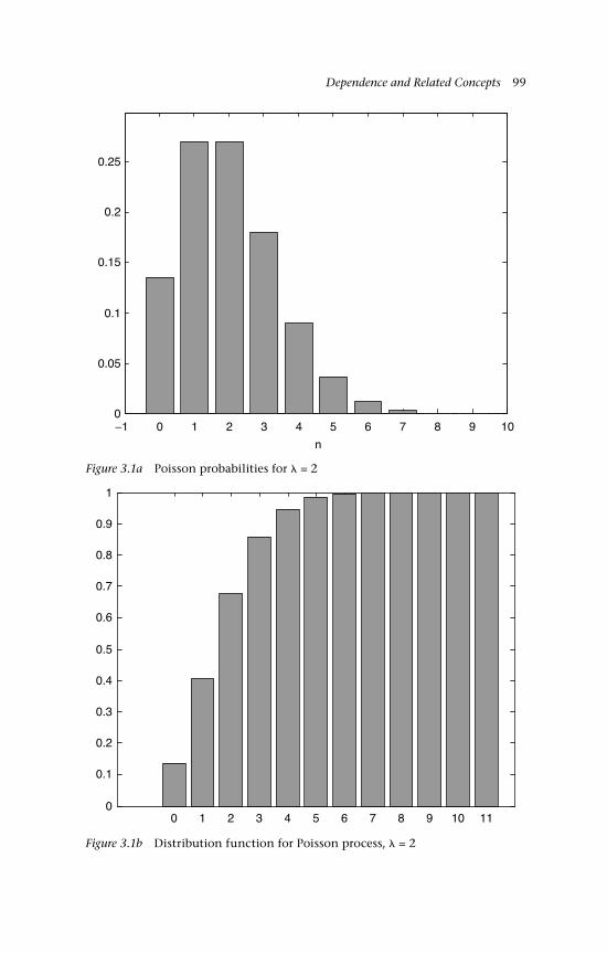
Dependence and Related Concepts 99
−1 0 1 2 3 4 5 6 7 8 9 100
0.05
0.1
0.15
0.2
0.25
n
Figure 3.1a Poisson probabilities for = 2
Figure 3.1b Distribution function for Poisson process, = 2
0 1 2 3 4 5 6 7 8 9 10 110
0.1
0.2
0.3
0.4
0.5
0.6
0.7
0.8
0.9
1
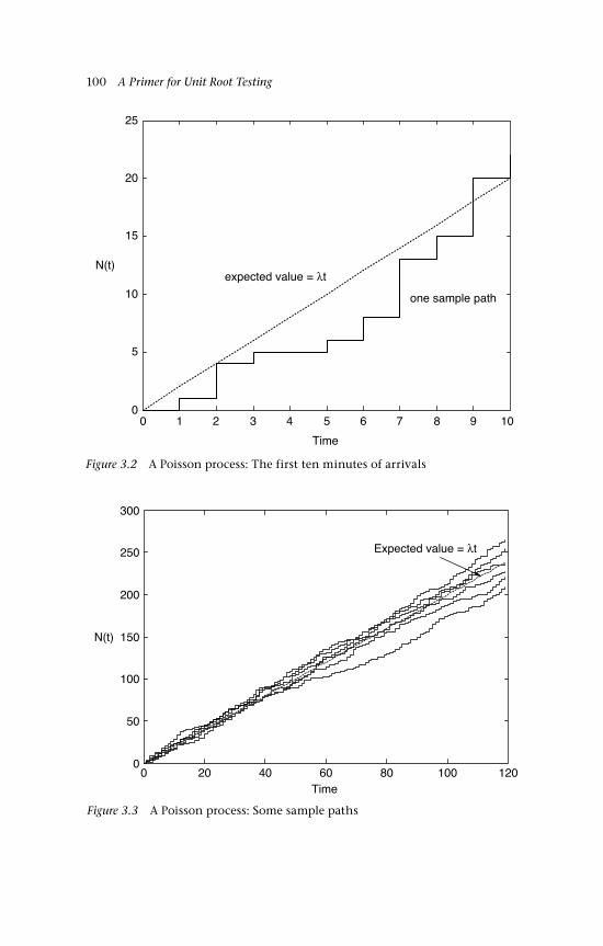
100 A Primer for Unit Root Testing
0 1 2 3 4 5 6 7 8 9 100
5
10
15
20
25
one sample path
Time
expected value = λtN(t)
Figure 3.2 A Poisson process: The first ten minutes of arrivals
Figure 3.3 A Poisson process: Some sample paths
0 20 40 60 80 100 1200
50
100
150
200
250
300
Time
N(t)
Expected value = λt
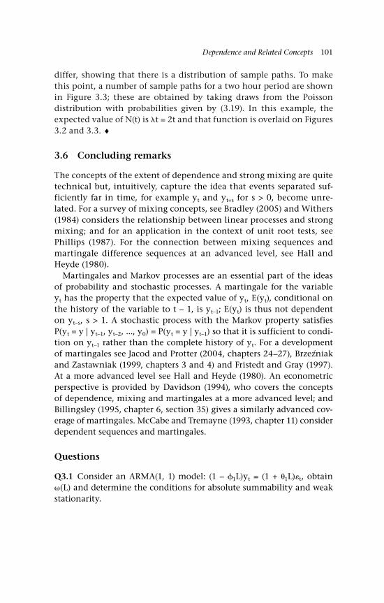
Dependence and Related Concepts 101
differ, showing that there is a distribution of sample paths. To make this point, a number of sample paths for a two hour period are shown in Figure 3.3; these are obtained by taking draws from the Poisson distribution with probabilities given by (3.19). In this example, the expected value of N(t) is t = 2t and that function is overlaid on Figures 3.2 and 3.3. ♦
3.6 Concluding remarks
The concepts of the extent of dependence and strong mixing are quite technical but, intuitively, capture the idea that events separated suf-ficiently far in time, for example yt and yt+s for s > 0, become unre-lated. For a survey of mixing concepts, see Bradley (2005) and Withers (1984) considers the relationship between linear processes and strong mixing; and for an application in the context of unit root tests, see Phillips (1987). For the connection between mixing sequences and martingale difference sequences at an advanced level, see Hall and Heyde (1980).
Martingales and Markov processes are an essential part of the ideas of probability and stochastic processes. A martingale for the variable yt has the property that the expected value of yt, E(yt), conditional on the history of the variable to t – 1, is yt–1; E(yt) is thus not dependent on yt–s, s > 1. A stochastic process with the Markov property satisfies P(yt = y | yt–1, yt–2, ..., y0) = P(yt = y | yt–1) so that it is sufficient to condi-tion on yt–1 rather than the complete history of yt. For a development of martingales see Jacod and Protter (2004, chapters 24–27), Brzezniak and Zastawniak (1999, chapters 3 and 4) and Fristedt and Gray (1997). At a more advanced level see Hall and Heyde (1980). An econometric perspective is provided by Davidson (1994), who covers the concepts of dependence, mixing and martingales at a more advanced level; and Billingsley (1995, chapter 6, section 35) gives a similarly advanced cov-erage of martingales. McCabe and Tremayne (1993, chapter 11) consider dependent sequences and martingales.
Questions
Q3.1 Consider an ARMA(1, 1) model: (1 – 1L)yt = (1 + 1L)t, obtain (L) and determine the conditions for absolute summability and weak stationarity.
102 A Primer for Unit Root Testing
A3.1 Assume that the ARMA(1, 1) model is causal, thus:
y L L
L L L
L
t t
t
jj
tj
= − +
= + + + +
=
−
−
=
∞
( ) ( )
( ) ( )
1 1
1 11
11
1 12 1
1
0
∑∑
This model was considered in example 2.2, where it was shown that j = 1
j–1 (1 + 1) for j ≥ 1, thus making the substitutions:
| | | ( ) |
| || ( ) |
jj
j
j
j
j
=
∞ −=
∞
−=
∞
∑ ∑∑
= + +
= + +
0 11
1 11
11
1 11
1
1 usinng |ab| |a||b|=
= + +
= + +
=
∞
=
∞
∑1
1
1 1 10
1 1 10
| || ( ) |
| ( ) | | |
j
j
j
j∑∑ +
= ++
−<
=−
as is a constant
if
| ( ) |
| ( ) || |
| |
|
1 1
1 1
111
11
1 11 1 1
1
1 1 12
1
1
1
1
| | ( ) || |
| | ( )
| |( )
+ +−
=− + +
−= +
using |a + b| a b 22
Hence, j=0 | j | = c < ∞ for | 1 | < 1. This is the same result that obtains
for the AR(1, 0) model. The presence of the MA(1) coefficient (and more generally the MA(q) coefficients), just serves to scale the magnitude of the response.
Note that if |(1 + 1)| = (1 + 1) > 0 and 1 > 0, then:
| |
( )
jj=
∞∑ = − + +−
= +−
=
01 1 1
1
1
1
11
11
1
Further, using results 3) and 4) from Section 3.4, yt is ergodic and weakly (or covariance) stationary; the qualification asymptotic may be neces-sary depending on how the initial value is determined in starting the AR(1) part of the process, see Section 3.2.
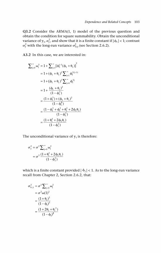
Dependence and Related Concepts 103
Q3.2 Consider the ARMA(1, 1) model of the previous question and obtain the condition for square summability. Obtain the unconditional variance of yt, y
2, and show that it is a finite constant if | 1 | < 1; contrast y
2 with the long-run variance 2lr,y
(see Section 2.6.2).
A3.2 In this case, we are interested in:
jj
j
j
j
j
2
0 11
1 11
2
1 12
12 1
1
1
1
1
=
∞ −=
∞
−=
∞
∑ ∑∑
= + +
= + +
= +
[ ( )]
( ) ( )
(( )
( )( )
( ) ( )(
1 12
12
0
1 12
12
12
1 12
1
11
11
+
= + +−
= + + +−
=
∞∑ j
j
22
12
12
12
1 1
12
12
1 1
12
1 21
1 21
)
( )( )
( )( )
= − + + +−
= + +−
The unconditional variance of yt is therefore:
y jj
2 2 2
0
2 12
1 1
12
1 21
=
=+ +
−
=
∞∑( )
( )
which is a finite constant provided | 1 | < 1. As to the long-run variance recall from Chapter 2, Section 2.6.2, that:
lr y jj,
( )
( )( )
( )( )
2 2 2
0
2 2
12
12
1 12
1
1
11
1 21
=
=
=+−
=+ +
−
=
∞∑
22

104 A Primer for Unit Root Testing
(Extension: note that it is not necessarily the case that 2lr,y > y
2; hence obtain the conditions for this inequality to hold.)
Q3.3 Let Y = (y1, y2, ..., yT) be a martingale with respect to the natural filtration; and assume that yt has a finite second moment. Show that E S E yT tt
T( ) ( )2 2
1=
=∑ .
A3.3 Note that S yT tt
T=
=∑ 1, hence:
E S y
E y E y y
T tt
T
tt
T
t t kt k
T
k
T
( ) var
( ) ( )
2
1
2
1 11
12
= ( )= +
=
= −= +=
−
∑∑ ∑∑
As to the last term, the application of three rules gives the result that E(ytys) = 0, s = t – k, k > 0:
E y y E S S S S
E E S S S St s t t s s
t t s s
( ) ( )( )
[( )( ) | ]
= − −
= − −− −
− −−
1 1
1 1 01Ft
== − −
= − −− −
−
−−
E S S E S S
E S S E S Es s t t
t t t
[( ) [( ) | ]
( )[ ( | ) (1 1 0
1
1 01
F
F
t
t SSt−− −
=1 0
10
1
0
| ) | ]F Ft t
As to the detail, the second line follows by the law of iterated expecta-tions (see Chapter 1). Let w be a random variable and F a conditioning field, then E[E(w | F)] = E(w). To apply this result let w = (Ss – Ss–1)(St – St–1) and F = F0
t–1.The third line is an application of ‘taking out what is known’. The
general result is E(xz | F) = xE(z | F) where x and z are random variables and x is F-measurable. Set x = (Ss – Ss–1) and z = (St – St–1), then applying the general result noting that s < t, gives:
E S S S S S S E S Ss s t t s s t t[( )( )| ] ( ) [( )| ]− − = − −− −−
− −−
1 1 01
1 1 01F Ft t
The last line follows because E S St t( | )Ft0
11
−−= from the defining con-
dition of a martingale, and E S St t( | )−−
−=1 01
1Ft as F0t–1 includes St–1, hence
E S E S S St t t( | ) ( | )1 01
1 01
1 1 0F Ft t−−
−− −− = − = .
The martingale result is, therefore, E S E yt jj
t( ) ( )2 2
1=
=∑ . The importance of the result is that it does not require that the yj are iid. This answer has drawn on McCabe and Tremayne (1993) and Hayashi (2000).
4Concepts of Convergence
105
Introduction
The idea of convergence is an important one in econometrics. Quite often it is not possible to determine the finite sample properties of, for example, the mean or distribution, of a random variable, such as an estimator or a test statistic; but in the limit, as the sample size increases, these properties are more easily determined. There is, however, more than one concept of convergence and different concepts may be appli-cable in different circumstances.
The matter of convergence is more complex in the case of a sequence of random variables compared to a nonstochastic sequence, since a ran-dom variable has multiple outcomes. There are some intuitively appeal-ing concepts of convergence; for example, perhaps we could require two random variables xn and x to be exactly the same in the limit, so that the probability of an event ω ∈ Ω in the probability space of the random variable xn is exactly the same as for the random variable x, and this holds for all ω. This would require that xn and x are defined on the same probability space. Overall, this is a stringent condition for convergence and some lesser form of convergence may well be sufficient for practical purposes.
Starting at the other end of the spectrum, we could ask what is the minimum form of convergence that would be helpful for a test statistic to satisfy in the event that the finite sample distribution is analytical intractable or difficult to use. In this case what it would be helpful to know is: what distribution does the distribution of xn, the n-th random variable in a sequence or ‘family’ of random variables, converge to in the limit, if one exists? Even when we know the finite sample distribu-tion, the limit distribution may be easier to use, an example being the
106 A Primer for Unit Root Testing
normal approximation to the binomial distribution, which works well even for moderate n when p and q are reasonably equal. Convergence in distribution turns out to be the weakest form of convergence that is sensible and useful. Another form of convergence that is in widespread use, which is stronger than convergence in distribution, is convergence in probability which gives rise to the much-used ‘plim’ notation; other concepts of convergence include almost sure convergence and conver-gence in mean square.
This chapter is organised as follows. Our central interest is in a sequence of random variables, for example, a test statistic indexed by the sample size, but, by way of introduction, Section 4.1 starts the chap-ter with a brief review of convergence concepts for a (nonstochastic) sequence of real numbers determined by a function of an index that may be increased without limit. Section 4.2 moves the concepts on to stochastic sequences and different concepts of convergence; this sec-tion includes an introduction to related results, such as the continu-ous mapping theorem (CMT), the central limit theorem (CLT), Slutsky’s theorem and the weak and strong laws of large numbers (WLLN and SLLN, respectively). A concept related to convergence (whether, for example, in distribution or probability) is the order of convergence which, loosely speaking, is a measure of how quickly sequences con-verge (if they do); again this idea can be related to nonstochastic or stochastic sequences and both are outlined in Section 4.3. Finally, the convergence of a stochastic process as a whole that is viewed not as the n-th term in a sequence, but of the complete trajectory, is considered in Section 4.4.
4.1 Nonstochastic sequences
Let xjnj=1 be a sequence of real numbers. Then the limit of the sequence
is x if,
for every ε > 0, there is an integer N, such that: |xn – x| < ε for n > N (4.1)
This is usually written as limn→ xn = x or xn → x; or equivalently limn→ |xn – x| = 0, see, for example, Pryce (1973).
Just as we may define a sequence of real numbers xjnj=1, we may define
a sequence of scalar functions. Let fj(x) be a scalar function that maps x ∈ S into the real line, , that is fj(x) : S → , then fj (x)n
j=1 is the associ-ated sequence of such functions.
Concepts of Convergence 107
The sequence fj(x)converges pointwise to f(x) if,
for every ε > 0 and every x ∈ S, there is an integer N: such that |fn(x) – f(x)| < ε for n > N (4.2)
Example 4.1: Some sequences
The following examples illustrate the two concepts of convergence.
Sequences of real numbers:
Example 1: xj = j does not converge;Example 2: xj = 1/j this is the sequence 1, 1/2, 1/3, which converges to
x = 0;Example 3: xj = (–1)j this is the sequence –1, 1, –1, ... , which does not
converge;Example 4: xj = (–1)2j this is the sequence 1, 1, 1, 1, ... , which does
converge to 1.
Sequence of scalar functions:
Example 5: fj(x) = xj converges to f(x) = 0 for | x | < 1, converges to f(x) = 1 for x = 1; alternates +1, –1 for x = –1; does not converge for | x | > 1. ♦
Given the sequence xjnj=1, then another sequence can be obtained as
the partial sum process, psp, of the original terms; that is Sjnj=1 where
Sj = ji=1xi. Convergence then refers to the property in terms of Sn and
convergence implies that limn→ Sn = S. The corresponding sequence of the partial sums does not necessarily have the same convergence prop-erty as its component elements. Consider some of the previous exam-ples (with an S to indicate the sum).
Example 4.2: Some sequences of partial sums
Example 1S: S jn j
n=
=∑ 1 does not converge
Example 2S: S jn j
n=
=∑ ( / )11
does not converge
Example 5S: S xnj
j
n=
=∑ 1 converges to x/(1 – x) for | x | < 1, but does not converge for | x | ≥ 1
Whilst it is obvious that example 2 converges, it may not be obvious that its partial sum analogue, example 2S, does not converge. The reader may recognise this as a harmonic series; the proof of its divergence has

108 A Primer for Unit Root Testing
an extensive history not pursued here. The interested reader is referred to Kifowit and Stamps (2006), who examine 20 proofs on divergence! Also note that in examples 5 and 5S, whilst xj = xj converges for x = 1, convergence of its psp requires | x | < 1. ♦
4.2 Stochastic sequences
More generally, it is random rather than deterministic sequences that will be of interest, so xj
nj=1 is now interpreted as a sequence of ran-
dom variables. A more explicit notation that emphasises this point is xj()n
j=1 but, generally, the simpler notation will be adequate. In prac-tice, the sequence of interest is often that of the partial sum proc-ess of xj, that is Sj
nj=1, or a scaled version of this sequence. When it
is the case that time is of the essence, then the time series notation St
Tt=1 will be preferred. In the case of random sequences or sequences
of random functions then, as noted in the introduction to this sec-tion, this raises some interesting questions about what convergence could be taken to mean when there is a possibly infinite number of outcomes. Four concepts of convergence are outlined in this section, together with related results.
4.2.1 Convergence in distribution (weak convergence): ⇒D
Consider the sequence of random variables xjnj=1, with a corresponding
sequence of distribution functions given by Fj(X)nj=1. Convergence in
distribution, or weak convergence, is the property that Fn(X) converges to F(X); that is:
lim ( ) ( )n nF X F X→∞ = (4.3)
or, in shorthand, Fn(X) ⇒D F(X). (The symbol ⇒ is sometimes used, but this notation is reserved here for ‘implication’, that is A ⇒ B, means A implies B.)
The weak convergence condition is qualified by adding that it holds for each X that is a continuity point of F(.); if there is a point, or points, of discontinuity in F(.), (4.3) is not required to hold at those points – broadly they are irrelevant (see example 14.4 of Billingsley, 1995). F(X) is referred to as the limiting distribution of the sequence. Although this form of convergence concerns the limiting distribution of xn, it is sometimes written in terms of the random variables as xn ⇒D x (or an equivalent notation), which should be taken as having the same meaning as (4.3).
Concepts of Convergence 109
That the definition (4.3) requires comment is evident on considering the nature of a distribution function, which could, for example, involve an infinity of values of X. The condition can equivalently be stated as:
lim ( ) ( )n nP x X P x X→∞ ≤ = ≤ (4.4)
for every continuity point X. Points of discontinuity in the limit dis-tribution function are excepted so that, for example, discrete limiting distributions are permitted, see McCabe and Tremayne (1993, chapter 3). As P(x X) [0, 1], the convergence of a distribution concerns the evaluation of ‘closeness’ in a sense that is familiar except, perhaps, for the idea that the evaluation is over a (possibly infinite) range of values (or points).
In the context of convergence in distribution, the probability spaces of xn and x need not be the same, unlike the concepts of convergence in probability and convergence almost surely that are considered below, as the following example shows.
Example 4.3: Convergence to the Poisson distribution
A well-known example of this kind, referred to in Chapter 3, Section 3.5.3, is the case of n Bernoulli trials, where each trial results in a 0 (‘failure’) or a 1 (‘success’). The probability space is the triple ( n, Fn, Pn). In n trials, the sample space, n, is the space of all n-tuples of 0s and 1s, = (1, ..., n), where j is either 0 or 1; the –field, Fn, is the field of all subsets of n; and the probability measure Pn assigns probability to each , comprising k successes and n – k failures in a sequence, as pk
n (1 – pn)n–k, where pn = /n. (The probability measure is as in Equations (3.25) and (3.26), with an appropriate change of notation and = 1). Let the random variable xn(), or simply xn, be the number, k, of successes in n trials, that is the number of 1s in a sequence of length n; then the probability mass function is that of the binomial distribution:
P x k C p pn n k nk
nn k( ( ) ) ( ) = = − −1 (4.5)
However, we have already seen that as n ∞, with pn = /n, the prob-abilities in (4.5) converge to those of the Poisson distribution, namely:
lim ( ( ) )( )
!( )
n n
k
P x k ek→∞
−= = (4.6)

110 A Primer for Unit Root Testing
The probability space for this random variable is that of a Poisson ran-dom variable. Thus, the Poisson distribution is the limiting distribution of a sequence of binomial distributed random variables; see Billingsley (1995, p. 330) and McCabe and Tremayne (1993, p. 53). (Note that in making the notational translation to Chapter 3, Section 3.5.3, use n for m and k for n.) ♦
4.2.2 Continuous mapping theorem, CMT
An important result in the context of convergence in distribution is the continuous mapping theorem, which states that:
if xn ⇒D x and P(x ∈ Dg) = 0, then g(xn) ⇒D g(x) (4.7)
where g(.) is a continuous function and Dg is the set of discontinuity points of g(.). For an elaboration, see Billingsley (1995, Theorem 25.7) and Davidson (1994 Theorem 22.11, 2000, Theorem 3.1.3). A familiar example from elementary texts is when x ∼ N(0, 1), and g(x) = x2, then g(x) has the 2(1) distribution; thus, if xn is asymptotically normal, then x2
n is asymptotically 2(1). An analogous result holds for convergence in probability, see Section 4.2.6.
4.2.3 Central limit theorem (CLT)
The CLT is a particularly important example of convergence in distri-bution. Let xj
nj=1 be a sequence of iid random variables with constant
mean and constant variance, that is, E(xj) = j = and 2(xj) = 2j = 2
x. Next consider Sn = n
j=1xj, which defines another sequence Sjnj=1; Sn will
have a mean of n and variance of n2x (by the iid assumption). Sn is
then standardised by subtracting its mean and dividing by its standard deviation:
zS n
nnn
x
= −
(4.8)
By the central limit theorem, the distribution function of zn, say F(Zn), tends to that of the standard normal as n → ∞; thus, F(Zn) ⇒D (Z), where the latter is the (cumulative) distribution function of the stand-ard normal random variable, with zero mean and unit variance, N(0, 1). Sometimes this convergence is written in terms of zn although, strictly, it applies to the cdf of zn; nevertheless, the same meaning is to be attrib-uted to zn ⇒D z, where z ∼ N(0, 1).
Concepts of Convergence 111
This result in Equation (4.8) can also be stated as n x Nn x( ) ( , )− ⇒ 0 2 , where x–n = n
i=1Sn/n, with the interpretation that the distribution of the average, x–n, converges to a random variable that is normally distributed with mean and variance 2
x /n, even though the component random variables are not normally distributed.
The assumption that xjnj=1 is a sequence of iid random variables is
sufficient rather than necessary for the CLT; for example, the CLT still goes through if xj
nj=1 is a martingale difference sequence, see Billingsley
(1995, p. 475). For generalisations and references, the interested reader is referred to Merlevède, Peligrad and Utev (2006) and to Ibragimov and Linnik (1971) for the extension to strict stationarity and strong mixing.
Example 4.4: Simulation example of CLT
In these examples, the sequence of interest is Sini=0, where Sj = n
j=1xj, and the xj are drawn from non-normal distributions. Specifically, there are two cases for the distribution of xj:
case 1: xj is a random variable with outcomes +1 and –1 with equal probability;
case 2: xj is a random variable uniformly distributed over [–1, +1].
The variance of xj = 1 for case 1, so that the appropriate standardisa-tion is zn = S nn / . The variance of a uniformly distributed random vari-able distributed over [a, b] is 2
unif = (b – a)2/12, so the standardisation for case 2 is z S nn n unif= /( ) ; for the simulations, b = +1 and a = –1, so that xj is centred on 0 and 2
unif = 1/3. The CLT applies to both of these distribu-tions; that is notwithstanding the non-normal inputs, in the limit zn ⇒D z, where z ~ N(0, 1).
Convergence in distribution (that is of the cdfs) implies that the cor-responding pdfs converge when they exist, as in this example. The results are illustrated for n = 20 and n = 200, with 10,000 replications used to obtain the empirical pdfs. Case 1 is shown in Figure 4.1 and case 2 in Figure 4.2; in each case, the familiar bell-shaped pdf of the stand-ardised normal distribution is overlaid on the graph. Considering case 1 first, the convergence is evident as n increases; for n = 20, the empirical pdf is close to the normal pdf and becomes closer as the sample size is increased to n = 200. The situation is similar for case 2, although the effect of the non-normal inputs is more evident for n = 20; however, the CLT is working clearly for n = 200. ♦

112 A Primer for Unit Root Testing
T = 20, +1/−1 inputs
−5 −4 −3 −2 −1 0 1 2 3 40
0.05
0.1
0.15
0.2
0.25
0.3
0.35
0.4
T = 200, +1/−1 inputsN(0, 1)
illustrating the CLT
Figure 4.1 Density estimates, +1, –1 inputs
−4 −3 −2 −1 0 1 2 3 40
0.05
0.1
0.15
0.2
0.25
0.3
0.35
0.4
0.45T = 20, uniform inputs T = 200, uniform inputsN(0, 1)
illustrating the CLT
Figure 4.2 Density estimates, uniform inputs
Concepts of Convergence 113
4.2.4 Convergence in probability: →p
Consider the sequence of random variables x1nj=1 and the single random
variable x defined on the same probability space. The random variable xn is said to converge in probability to x if, for all > 0, the following condition holds:
lim (| |n nP x x→∞ − < ) = 1 or, equivalently, lim (| | )n nP x x→∞ − ≥ = 0 (4.9)
This is written xn →p x, or some variant thereof; a common shorthand uses the ‘plim’ terminology, so that plim xn = x. It turns out to be help-ful to define the random variable w, such that w ≡ | xn – x |, so that the condition (4.9) can be stated as:
lim ( )n P w→∞ < = 1 or, equivalently, lim ( )n P w→∞ ≥ = 0 (4.10)
To illustrate what convergence in probability means, choose a ‘small’ value for , say = 0.1; then as n → ∞, it must be the case that Pn(w < 0.1) = 1. To visualise what is happening, consider a continuous random vari-able with a probability space on the positive half-line of real numbers, " = [0, ∞) (for example, this is the probability space for the square of a normally distributed variable), then the inequality w defines a subset w ∈ [0, 0.1). Convergence in probability requires that the probability of this subset tends to 1 as n increases. As this condition is required to hold for all positive then it must hold for = 0.01, = 0.001 and so on. In other words there must be an n such that the probability of even the slightest deviation of w from zero tends to one as n increases without limit. Convergence in probability implies convergence in distribution, but the reverse implication does not hold; indeed the distributions of xn and x need not be defined on the same probability space which, with the exception of convergence to a constant (see below) would rule out applicability of the concept.
Considering the joint distribution of two random variables, xn and x, McCabe and Tremayne (op. cit.,) note that the case that indicates convergence in probability is when the contours of the joint density are elongated around a 45° line with a slope of –1, indicating perfect cor-relation. A lack of association is indicated by contours that are circular, centred at zero. Indeed, this latter case is particularly instructive for if two variables are independent then one cannot converge to the other in probability, an example in point being two uncorrelated normal
114 A Primer for Unit Root Testing
distributed random variables since then a lack of correlation implies independence.
Example 4.5: Two independent random variables
The distribution of w depends on the joint distribution of xn and x, with a sample space that derives from the sample space of the two univari-ate distributions, as the following example shows. Let x and y denote independent random variables with each having the two outcomes 0 and 1, which occur with a probability ½; the random variables are, therefore, defined on the same sample space. Then the random variable x – y has three possible outcomes, which are: –1 with p(–1) = ¼, 0 with p(0) = ½ and 1 with p(+1) = ¼; hence, the random variable w = |x – y| has two possible outcomes, w = 0 with p(w = 0) = ½ and w = 1 with p(w = 1) = ½; see (Billingsley, 1995, section 25). ♦
4.2.5 Convergence in probability to a constant
A slightly modified form of convergence in probability occurs when xn converges in probability to a constant. The constant can be viewed as a degenerate random variable, such that x() = c for all ω ∈ Ω. In this case, the equivalent of the →p condition is:
lim (| | )n nP x c→∞ − < = 1 (4.11)
This condition is, therefore, one on the absolute value of the centred random variable xn – c. Because the xj do not have to be defined on the same probability space, Billingsley (1995, Theorem 25.3) sug-gests distinguishing this form of convergence from →p convergence; however, rather than introduce a separate notation, and in common with a number of texts, only one notation, that is →p, is used here. This case is also the exception in that convergence in distribution to a constant (that is to a degenerate distribution) implies convergence in probability.
4.2.6 Slutsky’s theorem
Let xn be the n-th term in the sequence xjn1, with xn →p c, and let
g(xn) be a continuous function, except on a set of measure zero, then g(xn) →p g(c). This is a very useful theorem as it is often relatively easy to determine the plim of xn by direct means, but less easy to obtain the plim of g(xn) in the same manner. Slutsky’s theorem shows how to do it quite simply.
Concepts of Convergence 115
A related theorem is the analogue of the CMT for convergence in probability. Let xn be the n-th term in the sequence xj
n1, with xn →p
x, and let g(x) be a continuous function of x, except on a set of meas-ure zero, then g(xn) →p g(x). In plim notation, plim g(xn) = g(x) and in words, ‘the probability limit of the function is the function of the prob-ability limit’, Fuller (1996, p. 222 and Theorem 5.1.4). This generalises Slutsky’s theorem by allowing the limit to be a random variable, rather than a constant.
4.2.7 Weak law of large numbers (WLLN)
A simple form of the weak law of large numbers is as follows. Consider again the sequence Sj
nj=1, where Sn = n
j=1xj and xj ~ iid (, 2x), as in the
CLT, and let x–n = Sn/n. Then for every ε > 0, the WLLN states:
lim (| | )n nP x→∞ − < = 1 (4.12)
This can be stated as x–n →p or plim x–n = . It provides a justification for using the average as an estimator of the population mean. In fact the conditions can be weakened quite substantially (as they are here sufficient for the strong law of large numbers, see below), whilst still achieving the same result; see, for example, Rao’s (1973) presentations of Chebyshev’s, Khinchin’s and Kolgomorov’s theorems.
4.2.8 Sure convergence
We start here from the concept of sure convergence, which although not generally used serves to underline the idea of almost sure conver-gence. Sure convergence is probably closest to an intuitive understand-ing of what is meant by convergence of a random variable. Recall that a random variable is a function that maps a sample space Ω into a meas-urable space, typically the set, or some subset, of the real numbers; for example, in tossing a coin, the outcomes heads and tails are mapped into the real numbers (0, 1) or (–1, +1). For each element in the sam-ple space, that is ∈ Ω, we could ask whether the measurable quantity xn() – x() is ‘large’; typically, negative and positive deviations are treated equally, so we could look at | xn() – x() | and ask whether this magnitude is less than an arbitrary ‘small’ number ε. It is somewhat unrealistic to expect this distance to be small for all values of the index n, but convergence would occur if ε = 0 in the limit as n → ∞, since then xn() = x(). An important feature of this kind of convergence is that it is being assessed for each ∈ Ω, so that it is sometimes referred to as element-wise (or point-wise) convergence; moreover, it does not then
116 A Primer for Unit Root Testing
make sense unless Ω is the sample space common to xn() and x(), for these are being compared element-by-element.
Sure convergence requires the following:
lim ( ) ( )n nx x→∞ = ∈ for all (4.13)
Clearly this is a strong notion of convergence and an interesting ques-tion is whether it can be weakened slightly, whilst still retaining the idea of element-wise convergence.
4.2.9 Almost sure convergence, →as
The answer is to take the probability of the limit, which leads to the concept of almost sure convergence, as follows:
P x xn n | lim ( ) ( ) ∈ = =→∞ 1 (4.14)
The corresponding shorthand notation is xn →as x. Sometimes statements are qualified as holding almost surely or, simply, a.s. See Stout (1974) for a detailed analysis of the concept of almost sure convergence.
The ‘almost’ refers to the following qualification to the condition. It does not apply to ∈ G ⊂ Ω where P(G) = 0, this is the ‘almost’; that is, there may be elements of Ω, in the subset G, for which convergence does not hold, but this does not matter provided that the probability of the set of such elements (if any) is zero. An example will illustrate this point and the idea of the concept.
Example 4.6: Almost sure convergence
The basic idea in this example is to define two random variables that differ only in a term that tends to zero as n → ∞, with the exception of some part of the sample space that has zero probability, which pro-vides the ‘almost’ sure part of convergence. With that aim, suppose that ∈ Ω = [0, ∞) and let xn() = + (1 + )–n
and x() = be two continuous random variables. Note that xn() → x() as n → ∞ for > 0; but xn(0) = 1 ≠ x(0) = 0 for any n. Thus, convergence is not sure; however, P( = 0) by the continuity of the pdf and, therefore, xn →as x. ♦
Note that convergence in probability makes a statement about the limiting probability, whereas almost-sure convergence makes a state-ment about the probability of the limit. Almost sure convergence is stronger than convergence in distribution and convergence in probabil-ity, and implies both of these forms of convergence.
Concepts of Convergence 117
4.2.10 Strong law of large numbers (SLLN)
Consider again the sequence Sjnj=1, where Sn = n
j=1xj and xj ~ iid (, 2), as in the CLT and the WLLN, and let x–n = Sn/n. Then for every ε > 0, the SLLN states:
P xn n(lim | | )→∞ − < = 1 (4.15)
Thus, there is almost sure convergence of x–n (‘the average’) to µ (‘the population mean’); that is, with probability 1, x–n converges to a con-stant, µ, as n → ∞; the assumptions on xj can be weakened quite sub-stantially, see, for example McCabe and Tremayne (1993) and Koralov and Sinai (2007).
4.2.11 Convergence in mean square and convergence in r-th mean: →r
Other concepts of convergence not covered in detail here include con-vergence in mean square, which is a special case of convergence in r-th mean. We note this case briefly. The sequence of random variables with n-th term xn converges in mean square to the random variable x, writ-ten xn →ms x or xn →r=2 x, if:
lim ( )n nE x x→∞ − =2 0 (4.16)
Thus, analogous to the elementary concept of variance, a measure of variation is the expected value of the squared difference between xn and the (limiting) random variable x, if this tends to zero with n, xn converges in mean square to x. This idea is extended in convergence in r-th mean, defined for xn as follows.
lim (| | )n nrE x x→∞ − = 0 (4.17)
As noted, the case with r = 2 is convergence in mean square as | | ( )x x x xn n− = −2 2. Otherwise the principle is the same, but the met-ric different, for different values of r. An intuitive case arises for r = 1, which might be described (loosely) as convergence in mean; consider the variable w = |xn – x|, which is the absolute difference between the two random variables (as in the case of convergence in probability), and necessarily non-negative, then if the expected value of w is zero in the limit, xn is said to converge to x in mean.
118 A Primer for Unit Root Testing
4.2.12 Summary of convergence implications
Convergence in r-th mean for r ≥ 1 implies convergence in probability and, hence convergence in distribution. The relationship between the convergence concepts is summarised in Table 4.1.
Table 4.1 Convergence implications
Almost surely In probability In distribution
xn →as x ⇒ xn →p x ⇒ xn ⇒D x
⇑xn →r x
In r-th mean
The reverse implications do not hold in general; however, an important exception is: if xn ⇒D c, where c is a constant, then xn →p c.
4.3 Order of Convergence
The order or magnitude of stochastic sequences is important at several stages in the development of unit root and stationarity tests. For exam-ple, consider a test statistic that is the ratio of two stochastic sequences. The asymptotic behaviour of the ratio, for example does it converge or diverge, depends on the order of convergence of the numerator and denominator components.
We start with the order of nonstochastic sequences as this is simply extended to stochastic sequences. Following mathematical convention, it is usual to use n, rather than t (or T), as an index for the last term in a sequence. This convention is followed in this section apart from where time series are being directly addressed.
4.3.1 Nonstochastic sequences: ‘big-O’ notation, ‘little-o’ notation
By way of example, consider two sequences with the n-th terms given by xn = a0 + a1n and yn = b0 + b1n + b2n2, where a0, a1, b0, b1 and b2 are constants. Both are unbounded as n → ∞, but require different normal-ising factors to reduce them to a bounded sequence in the limit. In the case of xn the required factor is n–1 and for yn it is n–2, so that:
n x a n a n x an n n−
→∞−= + =1
0 11
1/ limwith (4.18a)
n y b n b n b n y bn n n−
→∞−= + + =2
02
1 22
2/ / limwith (4.18b)
Concepts of Convergence 119
The sequences xn and yn are said to be of order n and n2, denoted O(n) and O(n2), respectively, read as order of magnitude; this is an example of the ‘big-O’ notation.
Note that all that matters when the function under examination comprises elements that are polynomials in n, is the dominant power of n. For example, if xn = K
kaknk, then the dominant term is aKnK and the sequence of which the n-th term is xn is O(nK).
More generally, to say that a sequence xn is O(n), written xn = O(n), means that:
lim| |
nnx
nc→∞ ≤ ≠ < ∞
0 (4.19)
Thus, the normalised sequence xn/n is bounded as n → ∞. Note that if division by n will ensure that a sequence is bounded, then so will division by, for example, n+1, n+2 and so on; therefore, implicit in the definition is the assumption that n is the minimum factor necessary to induce a bounded series; sometimes this is recognised by saying that xn is ‘at most of order’ n. Note that the order of magnitude necessarily refers to a sequence, although it is sometimes referred to without that qualification as applying to the n-th term, and written xn = O(n).
If xn and yn are to be reduced to zero rather than a non-zero constant, then the normalising factors have to be marginally greater than n, say n+, where ε > 0. For example, in the case of xn = a0 + a1n, which is O(n), division by n1+ results in:
xn
an
an
n( ) ( )1
01
1+ += +
(4.20)
so that lim ( )n nn x→∞
− + = >1 0 0 for .Generally, a sequence is said to be ‘of smaller order’ than n+, written
as xn = o(n+), if for some ε > 0, then the following holds:
limnnx
n→∞ + = >
0 0for (4.21)
Note that the definition is such that xn= O(n) ⇒ xn = o(n(")) for > 0. Conversely if a sequence is o(n) then it is O(n) for some ε > 0. In fact, if xn is o(n) then, by definition, it is also O(n), the bound being zero, but it is useful to capture the idea that an o(n) sequence dominates the xn sequence, whereas a O(n) sequence ‘matches’ the xn sequence.

120 A Primer for Unit Root Testing
There are two points to note on notation for order concepts. If the normalising factor is n0 ≡ 1, the convention is to write O(1) and o(1), respectively. The use of the equality symbol is not universal for these order concepts and here we follow, for example, Spanos (1986), Fuller (1976, 1996) and Davidson (1994); Hendry (1995), uses ≈, so that xn ≈ O(n) means the same as xn = O(n); in mathematical use, set notation is sometime used, for example xn ∈ O(n).
Generalising further, it may be the case that the normalising factor is something other than a power of n; for example, g(n) = log(n) or g(n) = loglog(n), in which case, the definitions of O(g(n)) and o(g(n)) are:
lim| |
( )nnx
g nc→∞ ≤ ≠ < ∞0 Xn = O(g(n)) (4.22)
lim( )n
nxg n→∞ = 0
Xn = o(g(n)) (4.23)
In both cases, the idea is the same as in the simpler case where only pow-ers of n were involved. Generally, in the case of O(g(n)), the sequence g(n) matches the xn sequence, whereas in the case of o((g(n)), the sequence g(n) dominates the xn sequence, both in the limit.
Lastly in this section and as an application of the ‘big-O’ notation, one possible explanation of a sustained movement in a time series is that there is a deterministic trend, so that a polynomial regression in time may be used as part of the analysis. For example, y tt j
j
j
K
t= +=∑
0,
where t is a stochastic input, is a simple form of a trend. In such cases, sums of the tj appear in the subsequent analysis and their order of mag-nitude is of interest. The most common cases are sums of linear and quadratic trends, respectively. These are:
t T T O T
t T T T O T
t
T
t
T
=
=
∑
∑
= + =
= + + =
1
2
2
1
3
12
1
16
1 2 1
( ) ( )
( )( ) ( )
Thus, in general, tK
t
T
=∑ 1 is O(TK+1). For a more comprehensive list and
analysis, see Banerjee et al. (1993).
4.3.2 Stochastic sequences: Op(n) and op(n)
The O(n) and o(n) definitions are extended to the case of stochastic sequences by considering the probability of ‘extreme’ events, see Mann and Wald (1943).
Concepts of Convergence 121
4.3.2.i At most of order n in probability: Op(n)
The analogue of O(n) is Op(n), read as at most of order n in probabil-ity. It is defined as follows: for any > 0, there exists a finite real number c(), such that for all n ≥ 1,
Pxn
cn| |( )
>
<
(4.24)
This is written as xn = Op(n), or sometimes without the braces around xn. In words, the probability of the absolute value of the n-th term in a bounded sequence exceeding the (finite) real number c() is less than . Consider the case of Op(1), then this implies that | xn | is bounded in probability by a number c(), such that:
P x cn| | ( )>( ) <
(4.25)
For example, suppose that xn is a random variable distributed as niid(0, 1) then, for all n ≥ 1, it is trivial to find a c() from standard normal tables, such that this inequality is satisfied. Notice that c(.) is written as a function of , since as changes then so, generally, will the value of c().
4.3.2.ii Of smaller order in probability than n: op(n)
Analogous to the o(n) case, xn is said to be of smaller order in probabil-ity than n, written xn = op(n) if:
limnnP
xn→∞
=
0
(4.26)
The op(1) case means that:
lim ( )n nP x→∞ = 0 (4.27)
The order notation is often used to indicate by how much, in terms of order of probability, xn differs from x; for example, if xn →p x then xn = x + op(1), which is to say that xn differs from x only in terms that are op(1) and thus tends to zero in the probability limit. A related result is that if xn ⇒D x, then xn = Op(1).
122 A Primer for Unit Root Testing
Example 4.7: O np( )
A case of particular importance is when x O nn p= ( ), so that:
Pxn
cn| |( )>
<
(4.28)
Thus, whilst xn is not bounded in probability, the scaled sequence with n-th term x nn / is bounded. To illustrate this case, consider the sequence of partial sums where Sn jj
n=
=∑ 1
, with j a random vari-able distributed as niid(0, 1). The variance of Sn is n2 = n, so that the standard deviation of Sn grows linearly with n . The normal-ised quantity S nn / is N(0, 1), which is Op(1), and, therefore, Sn is O np( ) .
To illustrate what the scaling is doing consider Figures 4.3 and 4.4, each of which has four sub-plots. The top panel of Figure 4.3 shows two realisations of Sn for n = 1, ... , 2,000, whereas the correspond-ing lower panel shows the same realisations scaled by n; whilst the paths of Sn are unbounded, those of S nn / are bounded (in probabil-ity). Then in Figure 4.4, the upper panel shows what happens when Sn is ‘overscaled’ by n rather than n ; the result is that Sn / n is close to the zero axis throughout. The lower panel shows that the distribu-tions of Sn / n for n = 1,000 and n = 2,000 approach a degenerate dis-tribution centred on zero, whereas S nn / is known to be distributed as N(0, 1). When n = 1,000 the probability of occurrences between ±0.05 is about 90%, and for n = 2,000 it is nearly 98%, indicating the converging degeneracy of the distributions. (The densities shown in the figure are estimated from 1,000 simulations of Sn for the two values of n.) ♦
4.3.3 Some algebra of the order concepts
Table 4.2 provides a summary of the relations between the order concepts for two sequences of nonstochastic or stochastic variables and is based on Mittlehammer (1996, lemma 5.2, p. 232). These rela-tionships also hold if O(.) and o(.) are replaced by Op(.) and op(.), respectively, and if more general functions, say (n) and (n) replace n and n.
Other relations of use include multiplication by a constant, : if xn = O(n), then xn = O(n), with similar results for o(n) and the stochastic equivalent. If xn is O(n) and yn is o(n), then xn/yn is o(n–).

Concepts of Convergence 123
Figure 4.4 Scaling by Sn by n produces a degenerate distribution
0 500 1000 1500 2000−0.5
0
0.5
0 500 1000 1500 2000−0.5
0
0.5
−0.5 0 0.50
2
4
6
8
10
12
−0.5 0 0.50
5
10
15
20
2nd sample path of Sn/n
Estimated density functions
approaches adegeneratedistribution
1st sample path of Sn/n
−100
−80
−60
−40
−20
0
20
−200
−150
−100
−50
0
50
0 1000 2000 3000 4000 5000−2
−1
0
1
2
0 1000 2000 3000 4000 5000
0 1000 2000 3000 4000 5000 0 1000 2000 3000 4000 5000
−3
−2
−1
0
1
2
scaling Sn by √n produces an Op(1) series
1st sample path of Sn 2nd sample path of Sn
Sn/√n Sn/√n
Figure 4.3 Appropriate scaling of a partial sum process
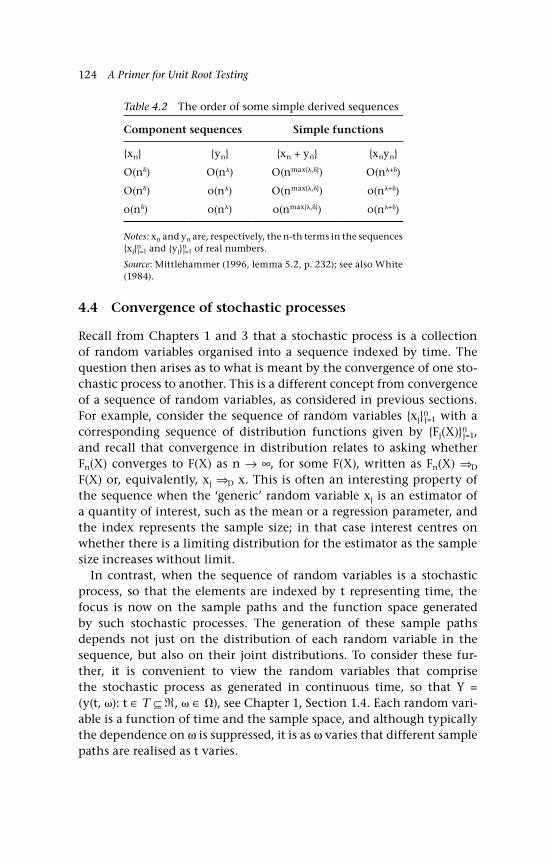
124 A Primer for Unit Root Testing
4.4 Convergence of stochastic processes
Recall from Chapters 1 and 3 that a stochastic process is a collection of random variables organised into a sequence indexed by time. The question then arises as to what is meant by the convergence of one sto-chastic process to another. This is a different concept from convergence of a sequence of random variables, as considered in previous sections. For example, consider the sequence of random variables xjn
j=1 with a corresponding sequence of distribution functions given by Fj(X)n
j=1, and recall that convergence in distribution relates to asking whether Fn(X) converges to F(X) as n → ∞, for some F(X), written as Fn(X) ⇒D F(X) or, equivalently, xj ⇒D x. This is often an interesting property of the sequence when the ‘generic’ random variable xj is an estimator of a quantity of interest, such as the mean or a regression parameter, and the index represents the sample size; in that case interest centres on whether there is a limiting distribution for the estimator as the sample size increases without limit.
In contrast, when the sequence of random variables is a stochastic process, so that the elements are indexed by t representing time, the focus is now on the sample paths and the function space generated by such stochastic processes. The generation of these sample paths depends not just on the distribution of each random variable in the sequence, but also on their joint distributions. To consider these fur-ther, it is convenient to view the random variables that comprise the stochastic process as generated in continuous time, so that Y = (y(t, ): t ∈ T ⊆ , ∈ ), see Chapter 1, Section 1.4. Each random vari-able is a function of time and the sample space, and although typically the dependence on ω is suppressed, it is as ω varies that different sample paths are realised as t varies.
Table 4.2 The order of some simple derived sequences
Component sequences Simple functions
xn yn xn + yn xnyn
O(n) O(n) O(nmax,) O(n+)
O(n) o(n) O(nmax,) o(n+)
o(n) o(n) o(nmax,) o(n+)
Notes: xn and yn are, respectively, the n-th terms in the sequences xjn
j=1 and yjnj=1 of real numbers.
Source: Mittlehammer (1996, lemma 5.2, p. 232); see also White (1984).

Concepts of Convergence 125
What can we say about the many (possibly infinite number of) sam-ple paths that could be generated in this way? It is clear that we would need to know not only about the distribution of each of the component random variables y(t), but also how they are related. The relationships between component random variables of the stochastic process are cap-tured by the joint distribution functions of Y:
P y t Y y t Yn n[ ( ) , , ( ) ]1 1≤ ≤ (4.29)
where t1 ≤ t2 ≤ ... ≤ tn, for all possible values of ti and n. These are the finite-dimensional distributions, or fidis, of the stochastic process. For example, we could specify a Gaussian stochastic process comprising independent N(0, 1) random variables. Such a process is generated with each component random variable having a (marginal) distribution that is N(0, 1) and each possible set of joint distributions is multivariate nor-mal, that is:
marginal distributions: y(ti) ~ N(0, 1) for all ti ∈ T (4.30a)
joint distributions (fidis):
P y t Y y t Y P y t Y P y t Y
P y t Yn n
n n
[ ( ) , , ( ) ] ( ( ) ) ( ( ) )
( ( ) )1 1 1 1 1 1≤ ≤ = ≤ ≤
≤ = ( ) ( ) ( )Y Y Yn1 2
(4.30b)
for all ti and n; and where (.) is the cdf of the standard normal distribu-tion and the assumption of independence is used in obtaining the joint distribution(s).
Whilst establishing the convergence of one stochastic process to another is more than just the convergence of the respective fidis, that is a good place to start. To that effect consider another stochastic process U = U(t1), ..., U(tn), with fidis given by:
P U t Y U t Yn n[ ( ) , , ( ) ]1 1≤ ≤ (4.31)
Then convergence of the finite-dimensional distributions occurs if for all tj, Yj and n, then:
P y t Y y t Y P U t Y U t Yn n D n n[ ( ) , , ( ) )] [ ( ) , , ( ) )]1 1 1 1≤ ≤ ⇒ ≤ ≤ (4.32)
126 A Primer for Unit Root Testing
The shorthand is Y ⇒D U, which says that the (joint) distribution of Y converges to the (joint) distribution of U. This is not sufficient by itself to enable us to say that one stochastic process converges to another; the additional condition is uniform tightness, a condition that is also required for a sequence of cdfs to have a cdf as its limit. The following statement of this condition is from Davidson (1994, section 22.5, see also sections 26.5 and 27.5). As in the concept of weak convergence let Ft(X) be a sequence of distribution functions indexed by t, then uniform tightness requires that for > 0, there exists a, b with b – a < ∞, such that:
sup ( ) ( )t T t tF b F a∈ − > −1 (4.33)
The condition (4.33) will fail for distributions that spread the density out too thinly over the support of the distribution, for example a uni-form distribution over an infinite interval (support) see Davidson (ibid). Subject to this point the convergence in (4.32) will be described as weak convergence and is the sense in which convergence of stochastic proc-esses is used in Chapters 6–8.
4.5 Concluding remarks and further reading
Convergence is a concept with wide applications in econometrics. Indeed, it is hard to make sense of the properties of estimators with-out knowledge of, for example, convergence in distribution (weak convergence) and convergence in probability (plim). In essence this form of convergence relates to the limiting behaviour of the n-th term in a sequence of random variables. A prototypical case would be a sequence of estimators of the same population quantity, for exam-ple a regression parameter or a test statistic, where the terms in the sequence are indexed by the sample size. Interest then centres on the limiting behaviour of the estimator as the sample size increases without limit.
Related to convergence is the ‘speed’ of convergence. By itself, conver-gence is uninformative about whether the approach to limiting quan-tity (distribution, scalar, random function) is slow or fast, it just says that as n → ∞, the limiting quantity is reached. However given two estimators of the same quantity, we would prefer the one that is quicker in approaching the limit. In this context it is of interest to know the order of convergence of the two estimators.
Concepts of Convergence 127
Once the groundwork of convergence of a sequence is achieved, it is possible to move onto the idea of the convergence of a stochastic process. The technical detail of this form of convergence is beyond the scope of this book, but much of the intuition derives from weak convergence and the convergence of the finite dimensional distributions.
For further reading, see Mittelhammer (1996) for an excellent treat-ment of the concepts of convergence and, for their application in a time series context, see Brockwell and Davis (2006). For the next level on stochastic processes, the reader could consult Mikosch (1998) and Brzezniak and Zastawniak (1999), McCabe and Tremayne (1993) and some parts of Billingsley (1995) and Davidson (1994). Classic texts on stochastic processes include Doob (1953) and Gihman and Skorohod (1974).
Questions
Q4.1 Show that n xn D( ) ( , )− ⇒ N 0 2 .
A4.1 Define zn as:
zS n
nnn=
−
Dividing the numerator and denominator by n gives:
zS n
n
x
n
nx
nn
n
nD
=−
=−
=−
⇒
( / )
/
/
( , )
N 0 1
Hence, n xn( ) ( , )− ⇒ N 0 2 .
Q4.2 Let x and y denote independent random variables, each with two outcomes, 0 and 1, which occur with a probability of ½. Are the follow-ing statements correct? i) x ⇒D y; ii) y ⇒D x; iii) x →p y (see Billingsley, 1995, section 25).
128 A Primer for Unit Root Testing
A4.2 Statements i) and ii) are correct, but iii) is not because P(|x – y| = 1) = ½, contradicting (4.9). (The sample space of |x – y| was considered in example 4.5: w = |x – y| has two possible outcomes, w = 0 and w = 1 each with a probability of ½.)
Q4.3 What are the O(.) and o(.) of xn, where:
xn n
nn =+ +
+4 3 2
6 1
2
?
A4.3 The only terms that matter asymptotically are 4n2/6n = (2/3)n, therefore xn = O(n), since [(2/3)n]/n = 2/3 As xn = O(n), then xn = o(n1+)for > 0, as [(2/3)n]/n1+ = (2/3)n → 0.
Q4.4 Consider the Taylor series expansion of the exponential:
e xx x xx = + + + + +12 3 4
2 3 4
! ! !...
For |x| < 1, what is the O(.) of the error in approximating ex by ignoring all terms in xk, k ≥ 4?
A4.4 Write the remainder from ignoring such higher order terms as R, so that:
e xx x
R
Rx
x = + + + +
= +
12 3
4
2 3
4
! !
!...
Note that R/x4 is:
Rx
x x4
214 5 6
= + + +! ! !
...
Given that |x| < 1, then xk > xk+1 and xk/(4 + k)! → 0 as k → ∞; hence R/x4 is bounded and, therefore, R = O(x4).
5An Introduction to Random Walks
129
This chapter introduces the idea of a random walk. In the first section, the emphasis is on the probability background of the random walk. It introduces the classic two-dimensional walk, primarily through the fiction of a gambler, which can be illustrated graphically. This serves two purposes, it underlies the motivation for the sample paths taken by some economic times series and it serves to introduce the partial sum (the gambler’s winnings), which is a critical quantity in subsequent econometric analysis. Some economic examples are given that confirm the likely importance of the random walk as an appropriate model for some economic processes.
The random walk is a natural introduction to Brownian motion, which is the subject of the next chapter, and is an example of a stochas-tic difference equation, in which the steps in the walk are driven by a random input. By making the steps in the walk smaller and smaller, the random walk can be viewed in the limit as occurring in continuous time and the stochastic difference equation becomes a stochastic dif-ferential equation. Equally, one might consider the random process as occurring in continuous time and the discrete-time version, that is the random walk, is what is observed.
This chapter is organised as follows. The basic idea of a random walk is introduced in Section 5.1, with some illustrative simulations of sym-metric random walks in Section 5.2 and some useful random walk probabilities in Section 5.3. Variations on the random walk theme are considered in Section 5.4. Some intuition about the nature of random walks is provided by looking at the variance of a partial sum process in Section 5.5 and the number of changes of sign on a random walk path in Section 5.6. Section 5.7 links random walks in with the presence of a unit root and Section 5.8 provides two examples.
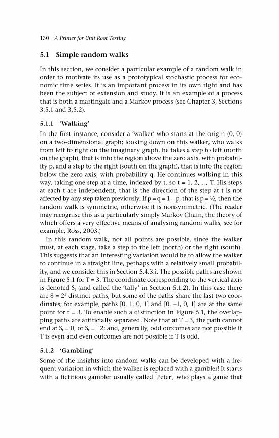
130 A Primer for Unit Root Testing
5.1 Simple random walks
In this section, we consider a particular example of a random walk in order to motivate its use as a prototypical stochastic process for eco-nomic time series. It is an important process in its own right and has been the subject of extension and study. It is an example of a process that is both a martingale and a Markov process (see Chapter 3, Sections 3.5.1 and 3.5.2).
5.1.1 ‘Walking’
In the first instance, consider a ‘walker’ who starts at the origin (0, 0) on a two-dimensional graph; looking down on this walker, who walks from left to right on the imaginary graph, he takes a step to left (north on the graph), that is into the region above the zero axis, with probabil-ity p, and a step to the right (south on the graph), that is into the region below the zero axis, with probability q. He continues walking in this way, taking one step at a time, indexed by t, so t = 1, 2, ... , T. His steps at each t are independent; that is the direction of the step at t is not affected by any step taken previously. If p = q = 1 – p, that is p = ½, then the random walk is symmetric, otherwise it is nonsymmetric. (The reader may recognise this as a particularly simply Markov Chain, the theory of which offers a very effective means of analysing random walks, see for example, Ross, 2003.)
In this random walk, not all points are possible, since the walker must, at each stage, take a step to the left (north) or the right (south). This suggests that an interesting variation would be to allow the walker to continue in a straight line, perhaps with a relatively small probabil-ity, and we consider this in Section 5.4.3.i. The possible paths are shown in Figure 5.1 for T = 3. The coordinate corresponding to the vertical axis is denoted St (and called the ‘tally’ in Section 5.1.2). In this case there are 8 = 23 distinct paths, but some of the paths share the last two coor-dinates; for example, paths [0, 1, 0, 1] and [0, –1, 0, 1] are at the same point for t = 3. To enable such a distinction in Figure 5.1, the overlap-ping paths are artificially separated. Note that at T = 3, the path cannot end at St = 0, or St = ±2; and, generally, odd outcomes are not possible if T is even and even outcomes are not possible if T is odd.
5.1.2 ‘Gambling’
Some of the insights into random walks can be developed with a fre-quent variation in which the walker is replaced with a gambler! It starts with a fictitious gambler usually called ‘Peter’, who plays a game that
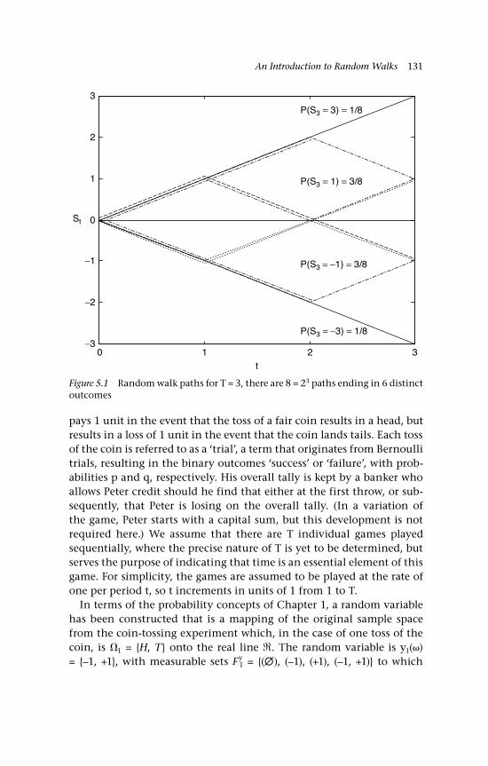
An Introduction to Random Walks 131
pays 1 unit in the event that the toss of a fair coin results in a head, but results in a loss of 1 unit in the event that the coin lands tails. Each toss of the coin is referred to as a ‘trial’, a term that originates from Bernoulli trials, resulting in the binary outcomes ‘success’ or ‘failure’, with prob-abilities p and q, respectively. His overall tally is kept by a banker who allows Peter credit should he find that either at the first throw, or sub-sequently, that Peter is losing on the overall tally. (In a variation of the game, Peter starts with a capital sum, but this development is not required here.) We assume that there are T individual games played sequentially, where the precise nature of T is yet to be determined, but serves the purpose of indicating that time is an essential element of this game. For simplicity, the games are assumed to be played at the rate of one per period t, so t increments in units of 1 from 1 to T.
In terms of the probability concepts of Chapter 1, a random variable has been constructed that is a mapping of the original sample space from the coin-tossing experiment which, in the case of one toss of the coin, is 1 = H, T onto the real line . The random variable is y1() = –1, +1, with measurable sets Fy
1 = (), (–1), (+1), (–1, +1) to which
0 1 2 3−3
−2
−1
0
1
2
3
t
P(S3 = 3) = 1/8
P(S3 = 1) = 3/8
St
P(S3 = −1) = 3/8
P(S3 = −3) = 1/8
Figure 5.1 Random walk paths for T = 3, there are 8 = 23 paths ending in 6 distinct outcomes
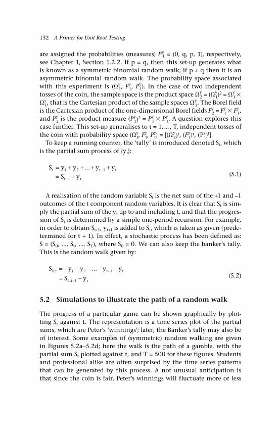
132 A Primer for Unit Root Testing
are assigned the probabilities (measures) Py1 = (0, q, p, 1), respectively,
see Chapter 1, Section 1.2.2. If p = q, then this set-up generates what is known as a symmetric binomial random walk; if p ≠ q then it is an asymmetric binomial random walk. The probability space associated with this experiment is (Ωy
1, Fy1, Py
1). In the case of two independent tosses of the coin, the sample space is the product space Ωy
2 = (Ωy1)
2 = Ωy1
Ωy1, that is the Cartesian product of the sample spaces Ωy
1. The Borel field is the Cartesian product of the one-dimensional Borel fields Fy
2 = Fy1 Fy
1, and Py
2 is the product measure (Py1)2 = Py
1 Py1. A question explores this
case further. This set-up generalises to t = 1, ... , T, independent tosses of the coin with probability space (Ωy
t, Fyt, P
yt) = [(Ωy
2)t, (Fy1)t, (Py
1)t].
To keep a running counter, the ‘tally’ is introduced denoted St, which is the partial sum process of yt:
S y y y y
S yt t t
t t
= + + + += +
−
−
1 2 1
1
...
(5.1)
A realisation of the random variable St is the net sum of the +1 and –1 outcomes of the t component random variables. It is clear that St is sim-ply the partial sum of the yt up to and including t, and that the progres-sion of St is determined by a simple one-period recursion. For example, in order to obtain St+1, yt+1 is added to St, which is taken as given (prede-termined for t + 1). In effect, a stochastic process has been defined as: S = (S0, ..., St, ..., ST), where S0 = 0. We can also keep the banker’s tally. This is the random walk given by:
S y y y y
S yB t t t
B t t
,
,
...= − − − − −= −
−
−
1 2 1
1 (5.2)
5.2 Simulations to illustrate the path of a random walk
The progress of a particular game can be shown graphically by plot-ting St against t. The representation is a time series plot of the partial sums, which are Peter’s ‘winnings’; later, the Banker’s tally may also be of interest. Some examples of (symmetric) random walking are given in Figures 5.2a–5.2d; here the walk is the path of a gamble, with the partial sum St plotted against t, and T = 500 for these figures. Students and professional alike are often surprised by the time series patterns that can be generated by this process. A not unusual anticipation is that since the coin is fair, Peter’s winnings will fluctuate more or less
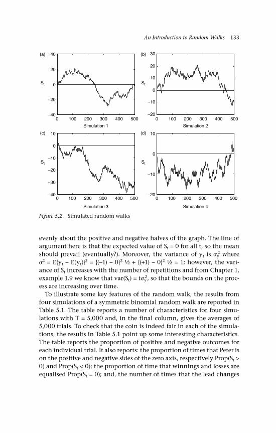
An Introduction to Random Walks 133
0 100 200 300 400 500−40
−20
0
20
40(a)
St
(c)
St
(b)
St
(d)
St
0 100 200 300 400 500−20
−10
0
10
20
30
0 100 200 300 400 500−40
−30
−20
−10
0
10
0 100 200 300 400 500−20
−10
0
10
Simulation 1 Simulation 2
Simulation 3 Simulation 4
Figure 5.2 Simulated random walks
evenly about the positive and negative halves of the graph. The line of argument here is that the expected value of St = 0 for all t, so the mean should prevail (eventually?). Moreover, the variance of yt is y
2 where 2 = Eyt – E(yt)2 = (–1) – 02 ½ + (+1) – 02 ½ = 1; however, the vari-ance of St increases with the number of repetitions and from Chapter 1, example 1.9 we know that var(St) = ty
2, so that the bounds on the proc-ess are increasing over time.
To illustrate some key features of the random walk, the results from four simulations of a symmetric binomial random walk are reported in Table 5.1. The table reports a number of characteristics for four simu-lations with T = 5,000 and, in the final column, gives the averages of 5,000 trials. To check that the coin is indeed fair in each of the simula-tions, the results in Table 5.1 point up some interesting characteristics. The table reports the proportion of positive and negative outcomes for each individual trial. It also reports: the proportion of times that Peter is on the positive and negative sides of the zero axis, respectively Prop(St > 0) and Prop(St < 0); the proportion of time that winnings and losses are equalised Prop(St = 0); and, the number of times that the lead changes
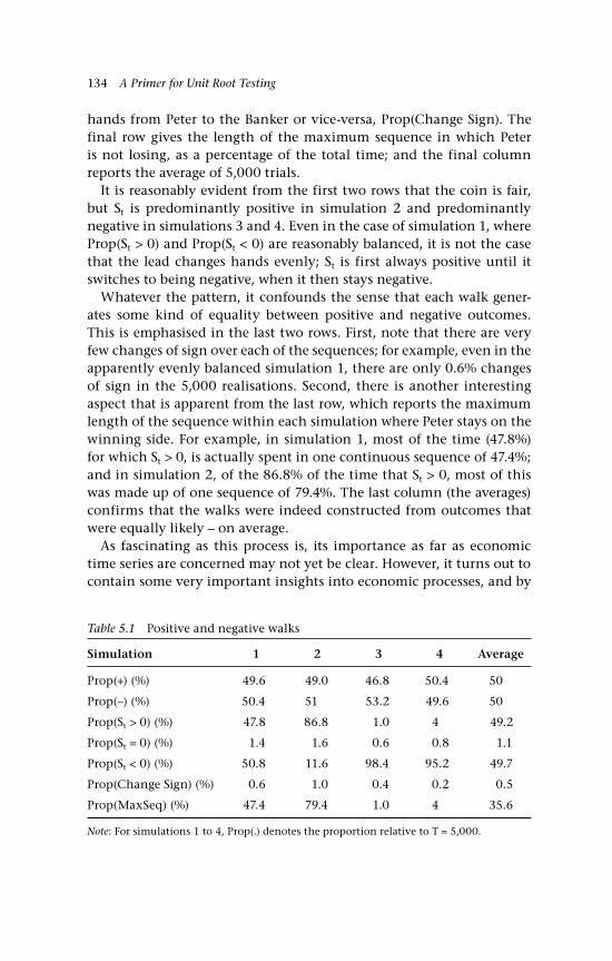
134 A Primer for Unit Root Testing
hands from Peter to the Banker or vice-versa, Prop(Change Sign). The final row gives the length of the maximum sequence in which Peter is not losing, as a percentage of the total time; and the final column reports the average of 5,000 trials.
It is reasonably evident from the first two rows that the coin is fair, but St is predominantly positive in simulation 2 and predominantly negative in simulations 3 and 4. Even in the case of simulation 1, where Prop(St > 0) and Prop(St < 0) are reasonably balanced, it is not the case that the lead changes hands evenly; St is first always positive until it switches to being negative, when it then stays negative.
Whatever the pattern, it confounds the sense that each walk gener-ates some kind of equality between positive and negative outcomes. This is emphasised in the last two rows. First, note that there are very few changes of sign over each of the sequences; for example, even in the apparently evenly balanced simulation 1, there are only 0.6% changes of sign in the 5,000 realisations. Second, there is another interesting aspect that is apparent from the last row, which reports the maximum length of the sequence within each simulation where Peter stays on the winning side. For example, in simulation 1, most of the time (47.8%) for which St > 0, is actually spent in one continuous sequence of 47.4%; and in simulation 2, of the 86.8% of the time that St > 0, most of this was made up of one sequence of 79.4%. The last column (the averages) confirms that the walks were indeed constructed from outcomes that were equally likely – on average.
As fascinating as this process is, its importance as far as economic time series are concerned may not yet be clear. However, it turns out to contain some very important insights into economic processes, and by
Table 5.1 Positive and negative walks
Simulation 1 2 3 4 Average
Prop(+) (%) 49.6 49.0 46.8 50.4 50
Prop(–) (%) 50.4 51 53.2 49.6 50
Prop(St > 0) (%) 47.8 86.8 1.0 4 49.2
Prop(St = 0) (%) 1.4 1.6 0.6 0.8 1.1
Prop(St < 0) (%) 50.8 11.6 98.4 95.2 49.7
Prop(Change Sign) (%) 0.6 1.0 0.4 0.2 0.5
Prop(MaxSeq) (%) 47.4 79.4 1.0 4 35.6
Note: For simulations 1 to 4, Prop(.) denotes the proportion relative to T = 5,000.
An Introduction to Random Walks 135
considering some of the ‘unexpected’ patterns that it generates we can find some motivation for considering it as prototypical stochastic proc-ess for economic data.
5.3 Some random walk probabilities
In this section we state and interpret some probabilities of interest, see especially Feller (1968, chapter III). Throughout this section, except where noted, we adopt the convention that n is defined such that 2n = T and t is, therefore, an index than runs over 1, ... , 2n (the exception is Equation (5.9) for changes of sign).
The first probability of interest is:
P S rC
h n rtn h
n( ) ( )/= = = +2
2where
(5.3)
This is the probability that at time t the partial sum St = r, |r| ≤ n. The binomial coefficient nCh (see below for definition) is assumed to be zero unless 0 ≤ h ≤ n is an integer.
Next is the probability that Peter is always winning. This is the prob-ability that St is everywhere positive:
P S SC
nn n
n( , , ) .1 22
20 0 0 52
> > =
(5.4)
The probability that Peter is never losing, which is the probability that St is never negative, is:
P S SC
nn n
n( , , )1 22
20 02
≥ ≥ =
(5.5)
The paths implied by the second and third probabilities share the first coordinate (1, 1), since Peter cannot lose on the first throw of the coin, but may differ as to the subsequent paths.
The binomial coefficient, as in (5.3), denoted nCh, is the number of ways of choosing h from n without regard to the order of choice. For example, nCh and 2nCn are, respectively:
n hCn
h n h=
−!
!( )! (5.6)
136 A Primer for Unit Root Testing
2
2
22
2
n nCn
n n n
nn
=−
=
( )!!(( ) )!
( )!( !)
(5.7)
where n! = n(n – 1)(n – 2) ... (1), read as ‘n factorial’.To illustrate these probabilities, let n = 2, so that 2n = T = 4, and the
relevant probabilities are as follows:
P S r CT r( ) ( ) ( )/= = −+2 4
4 4 2 for r ∈ A = [4, 2, 0, –2, –4] ⇒
P SC
P SC
P SC
T T T( ) ; ( ) ; ( )= =
= = =
= = − =02
38
22
14
24 24
4 34
4 1
2214
42
116
42
4
4 44
4 04
=
= =
= = − =
=
;
( ) ; ( )P SC
P SC
T T
1116
1; ( ) .P S rTr A= =
∈∑
P S SC
( , , ) .1 44 2
40 0 0 52
316
> > =
= ‘always winning’
P S SC
( , , )1 44 2
40 02
38
≥ ≥ =
= ‘never losing’
In a game consisting of 4 (sequential) tosses of a fair coin, the prob-ability that Peter is always winning is 3/16, and the probability that he is never losing is 3/8. Continuing the illustration, in the case of n = 5, so that T = 10, the respective probabilities are: 0.123 and 0.246. Already, these values might be quite surprising: the probability that Peter has not spent any time below the zero axis in ten tosses is just under ¼.
A related problem of interest, of which the last is a special case, is what fraction of the overall time Peter spends on the positive side of the axis. Intuition might suggest that this should be close to ½, but this is not the case. The formulation of the solution we use is due to Feller (1968, chapter III, Theorem 2 and corollary). It gives a general result that we can interpret as follows. Again let there be 2n = T sequential tosses at the rate of one per unit of time, t; define λ ≡ 2k/2n = k/n as the fraction of time Peter spends on the positive side; then k = 0 and k = n correspond to no time and all the time, respectively, with percentages of 0 and 100%.

An Introduction to Random Walks 137
In the time interval from t = 0, ... , = 2n = T, the probability that Peter spends exactly λ of the time on the positive side and, therefore, exactly (1 – λ) of the time on the negative side is given by:
PC C
k kk
n k n kn k( ) ( ) ( )
( ) =
− −−
22
222 2
(5.8a)
≈
−< <1 1
10 1
n
( ) (5.8b)
where ≈ indicates is approximately equal – see Feller (op. cit., Theorem 2) for details. Since k varies across all possible values, these probabilities must sum to unity. Further, the approximation, or direct calculation using Equation 5.8a shows that as n → ∞, the probability associated with a particular k tends to zero; hence, taking the integral to obtain the distribution function makes more sense and suggests that the cumula-tive probability is also of interest. The probability that the fraction of time spent on the positive side is less than or equal to λ is:
F P k nk n
( ) ( / )( / )
=≤∑
(5.9)
F() can be approximated by integrating the right-hand-side of (5.8b), so that:
F( ) sin
≅ −2 1
(5.10)
It may be helpful to illustrate some of these probabilities graphically. In the first case, we focus on P(S1 ! 0, ..., S2n ! 0) and allow n to vary; this is shown in Figure 5.3. This graph shows how the probability that Peter is never on the losing side varies as the number of trials increases. (In effect this is the graph for k = n, as n increases.) Thus, the probabili-ties are, sequentially: P(S1 ! 0, S2 ! 0) = 2/4 = ½, for n = 1; P(S1 ! 0, ..., S4 ! 0) = 6/16 = 3/8, for n = 2; and so on as n increases. Although these probabilities decline, they do so very slowly; for example, if n = 31, so that T = 62, then the probability that Peter never has a negative tally is 0.101; and even at n = 80 (T = 160), there is a 0.063 probability that Peter never has a negative tally.
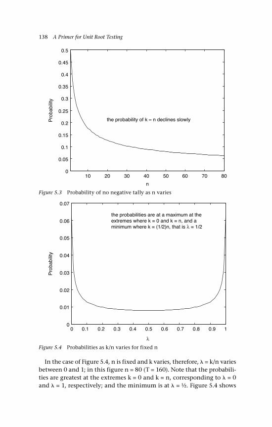
138 A Primer for Unit Root Testing
In the case of Figure 5.4, n is fixed and k varies, therefore, = k/n varies between 0 and 1; in this figure n = 80 (T = 160). Note that the probabili-ties are greatest at the extremes k = 0 and k = n, corresponding to = 0 and = 1, respectively; and the minimum is at = ½. Figure 5.4 shows
Figure 5.3 Probability of no negative tally as n varies
10 20 30 40 50 60 70 800
0.05
0.1
0.15
0.2
0.25
0.3
0.35
0.4
0.45
0.5
n
Pro
babi
lity
the probability of k = n declines slowly
Figure 5.4 Probabilities as k/n varies for fixed n
0 0.1 0.2 0.3 0.4 0.5 0.6 0.7 0.8 0.9 10
0.01
0.02
0.03
0.04
0.05
0.06
0.07
λ
Pro
babi
lity
the probabilities are at a maximum at theextremes where k = 0 and k = n, and aminimum where k = (1/2)n, that is λ = 1/2
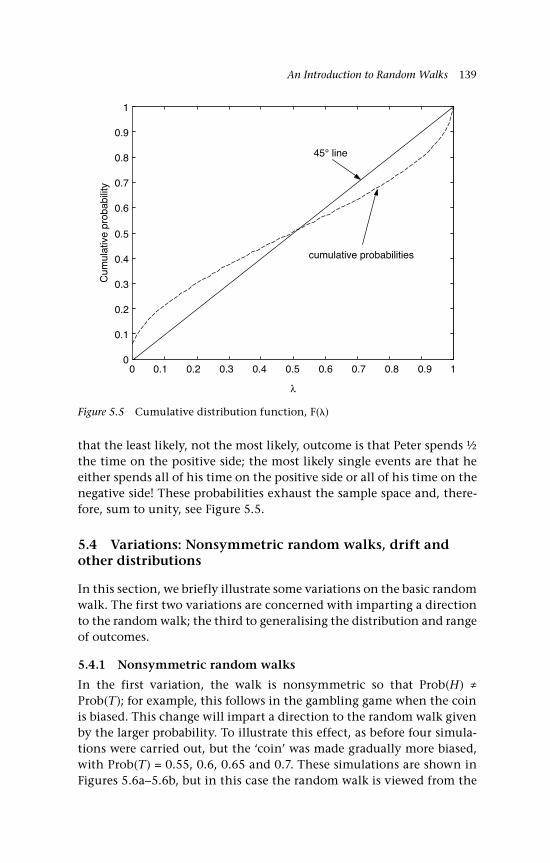
An Introduction to Random Walks 139
that the least likely, not the most likely, outcome is that Peter spends ½ the time on the positive side; the most likely single events are that he either spends all of his time on the positive side or all of his time on the negative side! These probabilities exhaust the sample space and, there-fore, sum to unity, see Figure 5.5.
5.4 Variations: Nonsymmetric random walks, drift and other distributions
In this section, we briefly illustrate some variations on the basic random walk. The first two variations are concerned with imparting a direction to the random walk; the third to generalising the distribution and range of outcomes.
5.4.1 Nonsymmetric random walks
In the first variation, the walk is nonsymmetric so that Prob(H) ≠ Prob(T); for example, this follows in the gambling game when the coin is biased. This change will impart a direction to the random walk given by the larger probability. To illustrate this effect, as before four simula-tions were carried out, but the ‘coin’ was made gradually more biased, with Prob(T) = 0.55, 0.6, 0.65 and 0.7. These simulations are shown in Figures 5.6a–5.6b, but in this case the random walk is viewed from the
Figure 5.5 Cumulative distribution function, F()
0 0.1 0.2 0.3 0.4 0.5 0.6 0.7 0.8 0.9 10
0.1
0.2
0.3
0.4
0.5
0.6
0.7
0.8
0.9
1
λ
Cum
ulat
ive
prob
abili
ty
cumulative probabilities
45° line
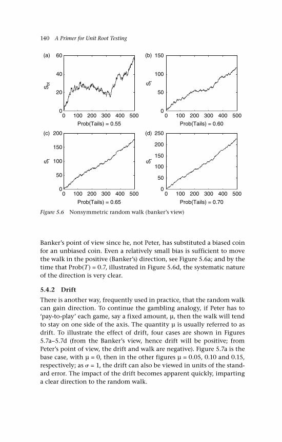
140 A Primer for Unit Root Testing
Banker’s point of view since he, not Peter, has substituted a biased coin for an unbiased coin. Even a relatively small bias is sufficient to move the walk in the positive (Banker’s) direction, see Figure 5.6a; and by the time that Prob(T) = 0.7, illustrated in Figure 5.6d, the systematic nature of the direction is very clear.
5.4.2 Drift
There is another way, frequently used in practice, that the random walk can gain direction. To continue the gambling analogy, if Peter has to ‘pay-to-play’ each game, say a fixed amount, µ, then the walk will tend to stay on one side of the axis. The quantity µ is usually referred to as drift. To illustrate the effect of drift, four cases are shown in Figures 5.7a–5.7d (from the Banker’s view, hence drift will be positive; from Peter’s point of view, the drift and walk are negative). Figure 5.7a is the base case, with µ = 0, then in the other figures µ = 0.05, 0.10 and 0.15, respectively; as = 1, the drift can also be viewed in units of the stand-ard error. The impact of the drift becomes apparent quickly, imparting a clear direction to the random walk.
0 100 200 300 400 5000
20
40
60
Sbt
0 100 200 300 400 5000
50
100
150
St
0 100 200 300 400 5000
50
100
150
200
St
0 100 200 300 400 5000
50
100
150
200
250
Prob(Tails) = 0.55 Prob(Tails) = 0.60
Prob(Tails) = 0.65 Prob(Tails) = 0.70
(a)
(c)
(b)
St
(d)
Figure 5.6 Nonsymmetric random walk (banker’s view)
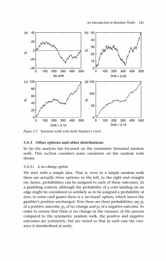
An Introduction to Random Walks 141
5.4.3 Other options and other distributions
So far the analysis has focussed on the symmetric binomial random walk. This section considers some variations on the random walk theme.
5.4.3.i A no-change option
We start with a simple idea. That is, even in a simple random walk there are actually three options: to the left, to the right and straight on; hence, probabilities can be assigned to each of these outcomes. In a gambling context, although the probability of a coin landing on an edge might be considered so unlikely as to be assigned a probability of zero, in some card games there is a ‘no-hand’ option, which leaves the gambler’s position unchanged. Now there are three probabilities, say p1 of a positive outcome, p2 of no change and p3 of a negative outcome. In order to ensure that there is no change in the variance of the process compared to the symmetric random walk, the positive and negative outcomes are symmetric, but are varied so that in each case the vari-ance is standardised at unity.
0 100 200 300 400 500−40
−20
0
20
40(a) (b)
(c) (d)
St
0 100 200 300 400 5000
10
20
30
40
50
0 100 200 300 400 5000
20
40
60
80
100
St
St
St
0 100 200 300 400 5000
50
100
150
No drift Drift = 0.05
Drift = 0.10 Drift = 0.15
Figure 5.7 Random walk with drift (banker’s view)
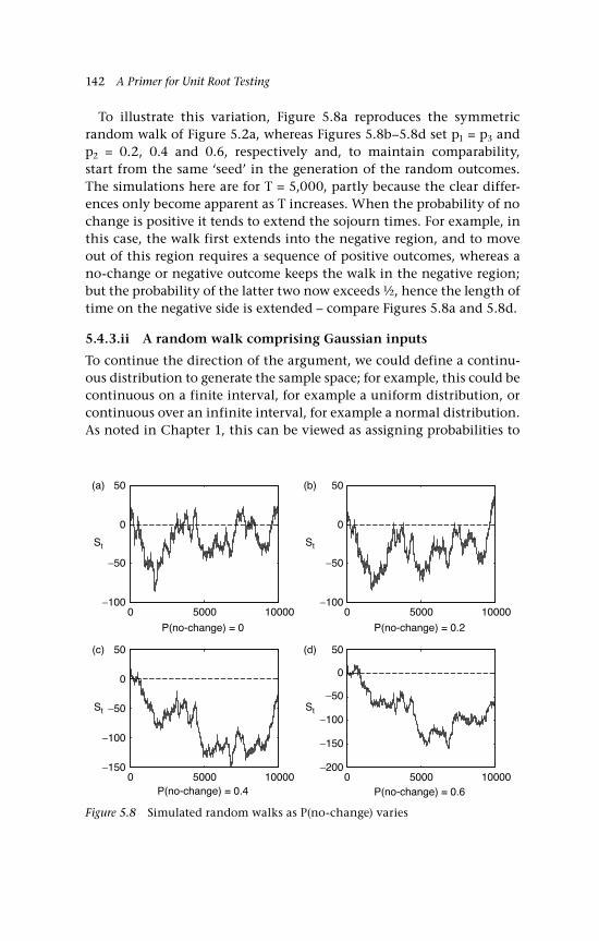
142 A Primer for Unit Root Testing
To illustrate this variation, Figure 5.8a reproduces the symmetric random walk of Figure 5.2a, whereas Figures 5.8b–5.8d set p1 = p3 and p2 = 0.2, 0.4 and 0.6, respectively and, to maintain comparability, start from the same ‘seed’ in the generation of the random outcomes. The simulations here are for T = 5,000, partly because the clear differ-ences only become apparent as T increases. When the probability of no change is positive it tends to extend the sojourn times. For example, in this case, the walk first extends into the negative region, and to move out of this region requires a sequence of positive outcomes, whereas a no-change or negative outcome keeps the walk in the negative region; but the probability of the latter two now exceeds ½, hence the length of time on the negative side is extended – compare Figures 5.8a and 5.8d.
5.4.3.ii A random walk comprising Gaussian inputs
To continue the direction of the argument, we could define a continu-ous distribution to generate the sample space; for example, this could be continuous on a finite interval, for example a uniform distribution, or continuous over an infinite interval, for example a normal distribution. As noted in Chapter 1, this can be viewed as assigning probabilities to
0 5000 10000−100
−50
0
50(a) (b)
(c) (d)
St
−100
−50
0
50
St
0 5000 10000
0 5000 10000−150
−100
−50
0
50
St
−200
−150
−100
−50
0
50
St
0 5000 10000
P(no-change) = 0 P(no-change) = 0.2
P(no-change) = 0.4 P(no-change) = 0.6
Figure 5.8 Simulated random walks as P(no-change) varies
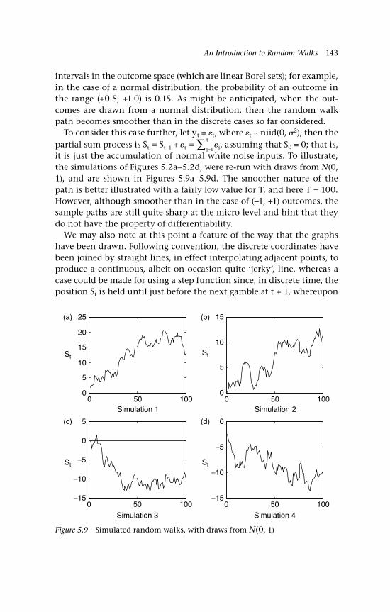
An Introduction to Random Walks 143
intervals in the outcome space (which are linear Borel sets); for example, in the case of a normal distribution, the probability of an outcome in the range (+0.5, +1.0) is 0.15. As might be anticipated, when the out-comes are drawn from a normal distribution, then the random walk path becomes smoother than in the discrete cases so far considered.
To consider this case further, let yt = t, where t ∼ niid(0, 2), then the partial sum process is S St t t jj
t= + =− =∑1 1
, assuming that S0 = 0; that is, it is just the accumulation of normal white noise inputs. To illustrate, the simulations of Figures 5.2a–5.2d, were re-run with draws from N(0, 1), and are shown in Figures 5.9a–5.9d. The smoother nature of the path is better illustrated with a fairly low value for T, and here T = 100. However, although smoother than in the case of (–1, +1) outcomes, the sample paths are still quite sharp at the micro level and hint that they do not have the property of differentiability.
We may also note at this point a feature of the way that the graphs have been drawn. Following convention, the discrete coordinates have been joined by straight lines, in effect interpolating adjacent points, to produce a continuous, albeit on occasion quite ‘jerky’, line, whereas a case could be made for using a step function since, in discrete time, the position St is held until just before the next gamble at t + 1, whereupon
0 50 100 0 50 1000
5
10
15
20
25(a) (b)
(c) (d)
St
0
5
10
15
St
0 50 100−15
−10
−5
0
5
St
0 50 100−15
−10
−5
0
St
Simulation 1 Simulation 2
Simulation 3 Simulation 4
Figure 5.9 Simulated random walks, with draws from N(0, 1)
144 A Primer for Unit Root Testing
the position St+1 is known; we continue with the convention, but return to this point in Chapter 6 where CADLAG functions are introduced.
5.5 The variance
Returning to the partial sum, it is evident that if yt ~ iid(0, 2y), yt ~
WN(0, 2y) or an MDS, then the variance of St evolves as t2
y. In general:
var( ) var( ) cov( ),S y y yt jj
t
i jj i
t
i
t= +
= >=∑ ∑∑1 12
(5.11)
So that if var(yj) = 2y and cov(yi, yj) = 0 for i ≠ j, then var(St) = t2
y. If the yt are heteroscedastic with cov(yi, yj) = 0, then the variance of St is:
var( ) var( )S yt jj
t=
=∑ 1 (5.12)
Again, this will increase with t.The covariances of the partial sums will also be of interest. We can
infer the general pattern from some simple examples. Recall from exam-ple 1.9 that:
cov( , ) cov( , ) cov( , ) cov( , )S S y y y y y yy2 32
1 2 1 3 2 32 2= + + +
If the covariances are zero, then:
cov(S2, S3) = 22y
In general, there are min(s, t) variances in common and the expecta-tion of all terms involving subscripts that are not equal will be zero by the iid, MDS or white noise assumption; hence, in general:
cov( , ) min( , )S S s ts t y= 2
(5.13)
Later we will also be interested in the variance of the differences in the partial sums, var(St – Ss). For convenience, assume that t > s, then the difference between these partial sums is just y y yjj
t
jj
s
jj s
t
= = = +∑ ∑ ∑− =1 1 1 , and,
hence, var( ) ( )S S t st s y− = − 2 .Figure 5.10 illustrates how the variance of the partial sums increases
with t, with values of var(St) from R = 1,000 replications of a walk of length T = 500, plotted against t. The random walk in this case is a

An Introduction to Random Walks 145
symmetric binomial random walk, with 2y = 1, but the pattern would
be almost indistinguishable with draws from niid(0, 1).To understand what these variances are, and what they are not, imag-
ine the data arranged into a T × R matrix; then there is a variance for each column and a variance for each row. The R column variances are the ‘sample’ variances, for which there is no theoretical counterpart; however, the T row variances have a well-defined theoretical coun-terpart in var(St) = t2
y = t, when, as here, 2y = 1. We can make the
correspondence of the simulated var(St) to t2y as good as we like by
increasing R. In this case R = 1,000 and the simulated var(St) are clearly very close to t (an exact correspondence would be a 45° line). Although the increase in the variance of the partial sum of a random walk is a clear identifying feature, in practice it is only a single column ‘sample’ variance that is available and that is not the appropriate concept; how-ever, tests of the random walk hypothesis can be based on a variance ratio, see for example Lo and MacKinlay (2001).
5.6 Changes of sign on a random walk path
In a sense to be made precise, there are few changes of sign in a ran-dom walk path, and this a one of its key distinguishing features. For
0 50 100 150 200 250 300 350 400 450 5000
50
100
150
200
250
300
350
400
450
500
t
theoretical variance:
Var(St) = tσ2 = t
simulation variance
based on 1,000 simulations
Figure 5.10 Simulation variance: var(St) as t varies

146 A Primer for Unit Root Testing
example, in the four illustrative simulations reported in Table 5.1 (and Figures 5.2a–5.2d), the maximum changes of sign was 1% in simulation 2. The average number of changes of sign in 5,000 trials was just 27 in a sample of T = 5,000 (0.54%).
A change of sign means that the path crosses the zero axis, which here marks the expected value of St; it is for this reason that a sign change is referred to as mean reversion. Thus, a frequent descriptive feature by which to broadly judge whether a path has been generated by a random walk, is to look for mean reversion or, equivalently, sign changes taking E(St) as the reference point. This heuristic also provides the basis of a test statistic for a unit root, see Burridge and Guerre (1996) and Garciá and Sansó (2006), which is developed in Chapter 8.
5.6.1 Binomial inputs
To make these ideas more precise we refer to Feller (1968, chapter III.5, Theorem 1) for the symmetric binomial random walk. A change of sign is dated at t if St–1 and St+1 are of opposite sign, in which case St = 0. (The identification of sign changes is slightly different if the underlying ran-dom variable is continuous.) The probability of k changes of sign in T realisations is given by:
2 2 1 22
P S kC
TT h
T( )= + =
(5.14)
where T = 2n + 1 and h = (2n + 2k +2) / 2 = (n + k + 1). As Feller (ibid) notes, this probability declines with k: thus, the largest probability is actually for no change of sign, which is illustrated for three choices of T = 99, 59 and 19 in Figure 5.11. The expected values of the number of sign changes are 3.48, 2.58 and 1.26, respectively.
Thus, it is incorrect to assume that the lead will change hands quite evenly. If this was the case then the graph of Peter’s winnings would show frequent crossings of the zero axis, but this event has negligible probability in a sense that can be made more precise as follows. Let #T k T= / be the normalised number of changes of sign in a symmetric binomial random walk starting at the origin, where k is the number of changes of sign and T the number of trials. Let F(#T) be the distribution function of #T for T trials. Then Feller (1968, chapter III.5, Theorem 2) derives the following limiting result as T → ∞:
F T D( ) ( )# #⇒ −2 2 1T (5.15)

An Introduction to Random Walks 147
where (.) is the cdf of the standard normal distribution (see Chapter 1, example 1.2). An equivalent statement in terms of the random vari-ables, rather than the distribution functions, is #T ⇒D $ where $ has the distribution given on the right of Equation (5.15). The limiting distribu-tion F(#T) is plotted in Figure 5.12 (solid line); it is, of course, defined only for # ≥ 0. The median is approximately 0.337, so that the median number of changes of sign for T trials is about 0 337. T ; for example if T = 100, then the median is about 3 (it has to be an integer). The limit-ing distribution is a remarkably good approximation for finite values of T. For example, the implied probabilities from the limit distribution and the exact probabilities from (5.14) for T = 19 are plotted in Figure 5.13 in the form of a bar chart; note that the bar heights are virtually indistinguishable.
In the case of a symmetric binomial random walk, just counting the sign changes will exclude the number of reflections; that is where the random walk reaches the zero axis, but it is reflected back in the same direction on the next step. In our sense this is also mean reversion as it is a ‘return to the origin’, although it is not a sign change. Since a change of sign implies a return to the origin, a count of mean rever-sions will include the sign changes; Burridge and Guerre (1996) note
0 2 4 6 8 10 12 14 160
0.05
0.1
0.15
0.2
0.25
0.3
0.35
0.4
k
Probability
T = 19
T = 99
T = 59
Figure 5.11 Probability of k sign changes
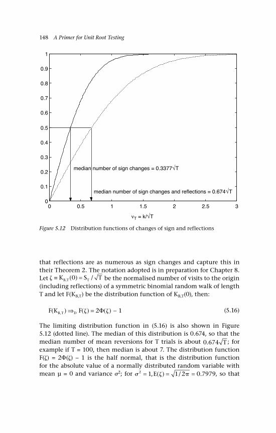
148 A Primer for Unit Root Testing
0 0.5 1 1.5 2 2.5 30
0.1
0.2
0.3
0.4
0.5
0.6
0.7
0.8
0.9
1
median number of sign changes = 0.3377√T
median number of sign changes and reflections = 0.674√T
νT = k/√T
Figure 5.12 Distribution functions of changes of sign and reflections
that reflections are as numerous as sign changes and capture this in their Theorem 2. The notation adopted is in preparation for Chapter 8. Let ≡ =K S TB T T, ( ) /0 be the normalised number of visits to the origin (including reflections) of a symmetric binomial random walk of length T and let F(KB,T) be the distribution function of KB,T(0), then:
F K FB T D( ) ( ) ( ), ⇒ = − 2 1 (5.16)
The limiting distribution function in (5.16) is also shown in Figure 5.12 (dotted line). The median of this distribution is 0.674, so that the median number of mean reversions for T trials is about 0 674. T ; for example if T = 100, then median is about 7. The distribution function F() = 2() – 1 is the half normal, that is the distribution function for the absolute value of a normally distributed random variable with mean µ = 0 and variance 2; for 2 1 1 2 0 7979= = =, ( ) / .E , so that
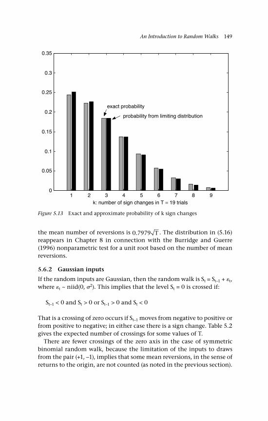
An Introduction to Random Walks 149
the mean number of reversions is 0 7979. T . The distribution in (5.16) reappears in Chapter 8 in connection with the Burridge and Guerre (1996) nonparametric test for a unit root based on the number of mean reversions.
5.6.2 Gaussian inputs
If the random inputs are Gaussian, then the random walk is St = St–1 + t, where t ~ niid(0, 2). This implies that the level St = 0 is crossed if:
St–1 < 0 and St > 0 or St–1 > 0 and St < 0
That is a crossing of zero occurs if St–1 moves from negative to positive or from positive to negative; in either case there is a sign change. Table 5.2 gives the expected number of crossings for some values of T.
There are fewer crossings of the zero axis in the case of symmetric binomial random walk, because the limitation of the inputs to draws from the pair (+1, –1), implies that some mean reversions, in the sense of returns to the origin, are not counted (as noted in the previous section).
1 2 3 4 5 6 7 8 90
0.05
0.1
0.15
0.2
0.25
0.3
0.35
k: number of sign changes in T = 19 trials
exact probability
probability from limiting distribution
Figure 5.13 Exact and approximate probability of k sign changes
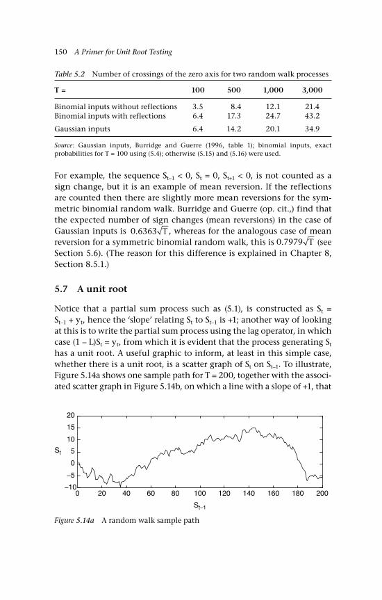
150 A Primer for Unit Root Testing
For example, the sequence St–1 < 0, St = 0, St+1 < 0, is not counted as a sign change, but it is an example of mean reversion. If the reflections are counted then there are slightly more mean reversions for the sym-metric binomial random walk. Burridge and Guerre (op. cit.,) find that the expected number of sign changes (mean reversions) in the case of Gaussian inputs is 0 6363. T , whereas for the analogous case of mean reversion for a symmetric binomial random walk, this is 0 7979. T (see Section 5.6). (The reason for this difference is explained in Chapter 8, Section 8.5.1.)
5.7 A unit root
Notice that a partial sum process such as (5.1), is constructed as St = St–1 + yt, hence the ‘slope’ relating St to St–1 is +1; another way of looking at this is to write the partial sum process using the lag operator, in which case (1 – L)St = yt, from which it is evident that the process generating St has a unit root. A useful graphic to inform, at least in this simple case, whether there is a unit root, is a scatter graph of St on St–1. To illustrate, Figure 5.14a shows one sample path for T = 200, together with the associ-ated scatter graph in Figure 5.14b, on which a line with a slope of +1, that
Table 5.2 Number of crossings of the zero axis for two random walk processes
T = 100 500 1,000 3,000
Binomial inputs without reflectionsBinomial inputs with reflections
3.56.4
8.417.3
12.124.7
21.443.2
Gaussian inputs 6.4 14.2 20.1 34.9
Source: Gaussian inputs, Burridge and Guerre (1996, table 1); binomial inputs, exact probabilities for T = 100 using (5.4); otherwise (5.15) and (5.16) were used.
Figure 5.14a A random walk sample path
0 20 40 60 80 100 120 140 160 180 200−10
−5
0
5
10
15
20
St
St−1
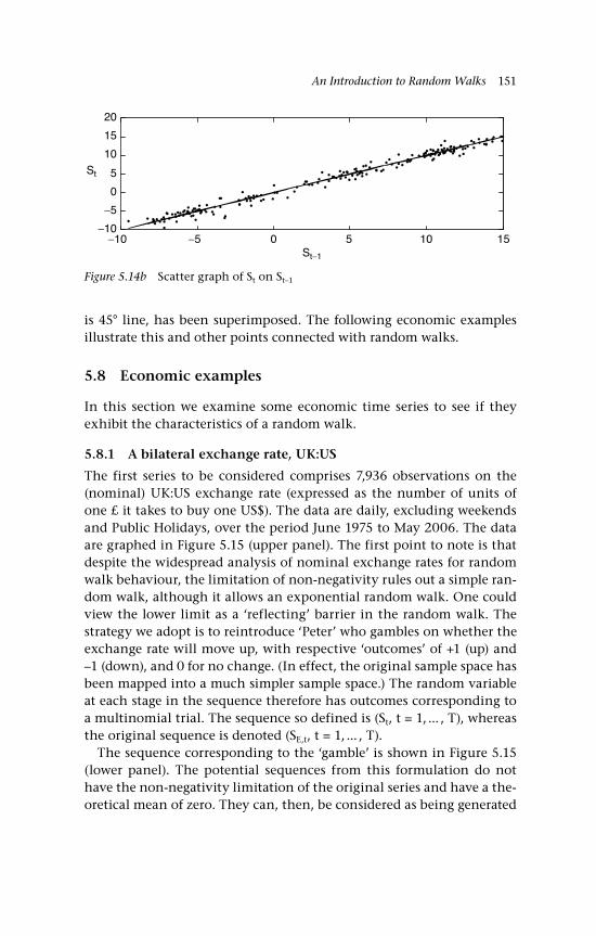
An Introduction to Random Walks 151
is 45° line, has been superimposed. The following economic examples illustrate this and other points connected with random walks.
5.8 Economic examples
In this section we examine some economic time series to see if they exhibit the characteristics of a random walk.
5.8.1 A bilateral exchange rate, UK:US
The first series to be considered comprises 7,936 observations on the (nominal) UK:US exchange rate (expressed as the number of units of one £ it takes to buy one US$). The data are daily, excluding weekends and Public Holidays, over the period June 1975 to May 2006. The data are graphed in Figure 5.15 (upper panel). The first point to note is that despite the widespread analysis of nominal exchange rates for random walk behaviour, the limitation of non-negativity rules out a simple ran-dom walk, although it allows an exponential random walk. One could view the lower limit as a ‘reflecting’ barrier in the random walk. The strategy we adopt is to reintroduce ‘Peter’ who gambles on whether the exchange rate will move up, with respective ‘outcomes’ of +1 (up) and –1 (down), and 0 for no change. (In effect, the original sample space has been mapped into a much simpler sample space.) The random variable at each stage in the sequence therefore has outcomes corresponding to a multinomial trial. The sequence so defined is (St, t = 1, ... , T), whereas the original sequence is denoted (SE,t, t = 1, ... , T).
The sequence corresponding to the ‘gamble’ is shown in Figure 5.15 (lower panel). The potential sequences from this formulation do not have the non-negativity limitation of the original series and have a the-oretical mean of zero. They can, then, be considered as being generated
Figure 5.14b Scatter graph of St on St–1
−10 −5 0 5 10 15−10
−5
0
5
10
15
20
St
St−1
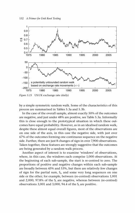
152 A Primer for Unit Root Testing
by a simple symmetric random walk. Some of the characteristics of this process are summarised in Tables 5.3a and 5.3b.
In the case of the overall sample, almost exactly 50% of the outcomes are negative, and just under 48% are positive, see Table 5.3a. Informally this is close enough to the prototypical situation in which these out-comes have equal probability. However, as in an idealised random walk, despite these almost equal overall figures, most of the observations are on one side of the axis, in this case the negative side, with just over 67% of the outcomes forming one continuous sequence on the negative side. Further, there are just 8 changes of sign in over 7,900 observations. Taken together, these features are strongly suggestive that the outcomes are being generated by a random walk process.
Another aspect of interest is to examine ‘windows’ of observations, where, in this case, the windows each comprise 1,000 observations. At the beginning of each sub-sample, the start is re-centred to zero. The proportions of positive and negative changes within each sub-sample are broadly between 45% and 53%, but there are relatively few changes of sign for the partial sum, St, and some very long sequences on one side or the other; for example, between (re-centred) observations 1,001 and 2,000, 97.8% of the St are negative, whereas between (re-centred) observations 3,001 and 3,000, 94.4 of the St are positive.
1975 1980 1985 1990 1995 2000 2005−200
−150
−100
−50
0
50
1975 1980 1985 1990 1995 2000 20050.4
0.5
0.6
0.7
0.8
0.9
1
£:$
a potentially unbounded random walkbased on exchange rate movements (+/−)
Figure 5.15 US:UK exchange rate (daily)

An Introduction to Random Walks 153
To illustrate, Figure 5.16 shows the scatter graph of SE,t on SE,t–1 for the last 1,000 observations, with a 45° line superimposed on the scatter. (The scatter is so dense around the line that the number of observations is limited; also using St rather than SE,t results in a similar plot.) The tightness of the scatter plot around the 45° line is evident, which sug-gests quite strongly that the exchange rate has the properties associated with a random walk.
5.8.2 The gold-silver price ratio
The second series to be considered is the ratio of gold to silver price, obtained from the daily London Fix prices for the period 2 January 1985 to 31 March 2006; weekends and Bank holidays are excluded, giving an overall total of T = 5,372 observations. Whilst either of these prices might be considered singly, they are nominal prices and it makes more economic sense to apply a numeraire, with the cost of gold in terms of silver well established in this respect.
Table 5.3a Characteristics of a sequence of gambles on the UK:US exchange rate
+ veoutcomes No-change
– veoutcomes
sign changes
Longest + sequence
Longest – sequence
Number 3,797 172 3,966 8 585 5,347
Proportion (%)
47.8 2.2 50.0 0.1 7.4 67.3
Table 5.3b Sub-samples of the sequence of gambles on the UK:US exchange rate
1,001–2,000
2,001–3,000
3,001–4,000
4,001–5,000
5,001–6,000
6,001–7,000
Prop(+) 48.3 51.2 44.7 48.7 49.1 49.4
Prop(=) 1.6 1.1 1.9 1.5 1.0 1.7
Prop(–) 50.1 47.7 53.4 49.8 49.9 48.9
Prop(St > 0) 0.1 97.1 0.8 65.5 27.7 98.1
Prop(St = 0) 0.3 0.4 1.1 4.9 2.6 0.3
Prop(St < 0) 99.6 2.5 98.1 29.6 69.7 1.6
Prop(Change Sign) 0.2 0.2 0.9 2.3 1.2 0.3
Prop(MaxSeq+) 0.1 94.4 0.5 25.3 21.9 97.8
Prop(MaxSeq–) 97.8 2.5 97.0 17.5 46.8 1.5
Note: overall data period, June 1975 to May 2006, comprising 7,936 observations.
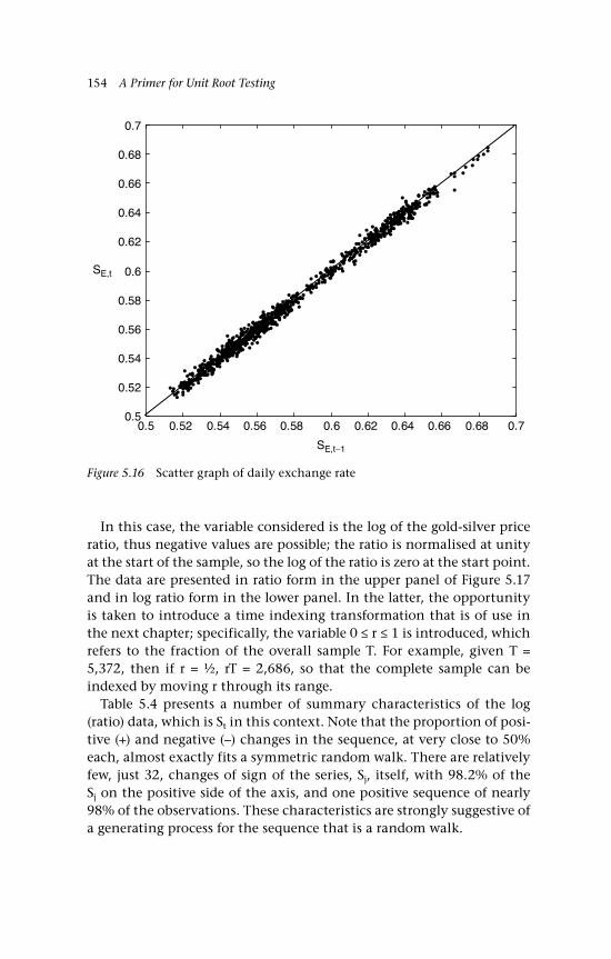
154 A Primer for Unit Root Testing
In this case, the variable considered is the log of the gold-silver price ratio, thus negative values are possible; the ratio is normalised at unity at the start of the sample, so the log of the ratio is zero at the start point. The data are presented in ratio form in the upper panel of Figure 5.17 and in log ratio form in the lower panel. In the latter, the opportunity is taken to introduce a time indexing transformation that is of use in the next chapter; specifically, the variable 0 ≤ r ≤ 1 is introduced, which refers to the fraction of the overall sample T. For example, given T = 5,372, then if r = ½, rT = 2,686, so that the complete sample can be indexed by moving r through its range.
Table 5.4 presents a number of summary characteristics of the log (ratio) data, which is St in this context. Note that the proportion of posi-tive (+) and negative (–) changes in the sequence, at very close to 50% each, almost exactly fits a symmetric random walk. There are relatively few, just 32, changes of sign of the series, Sj, itself, with 98.2% of the Sj on the positive side of the axis, and one positive sequence of nearly 98% of the observations. These characteristics are strongly suggestive of a generating process for the sequence that is a random walk.
0.5 0.52 0.54 0.56 0.58 0.6 0.62 0.64 0.66 0.68 0.70.5
0.52
0.54
0.56
0.58
0.6
0.62
0.64
0.66
0.68
0.7
SE,t
SE,t−1
Figure 5.16 Scatter graph of daily exchange rate
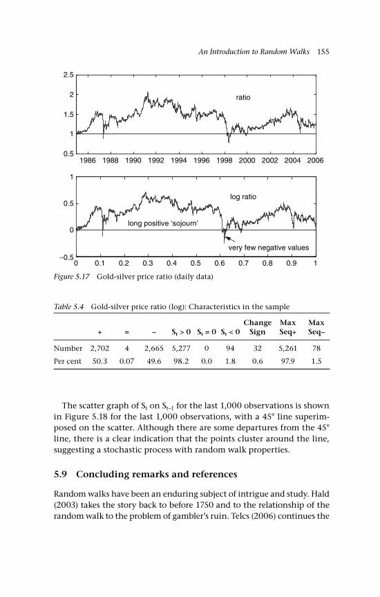
An Introduction to Random Walks 155
The scatter graph of St on St–1 for the last 1,000 observations is shown in Figure 5.18 for the last 1,000 observations, with a 45° line superim-posed on the scatter. Although there are some departures from the 45° line, there is a clear indication that the points cluster around the line, suggesting a stochastic process with random walk properties.
5.9 Concluding remarks and references
Random walks have been an enduring subject of intrigue and study. Hald (2003) takes the story back to before 1750 and to the relationship of the random walk to the problem of gambler’s ruin. Telcs (2006) continues the
Table 5.4 Gold-silver price ratio (log): Characteristics in the sample
+ = – St > 0 St = 0 St < 0Change
SignMaxSeq+
MaxSeq–
Number 2,702 4 2,665 5,277 0 94 32 5,261 78
Per cent 50.3 0.07 49.6 98.2 0.0 1.8 0.6 97.9 1.5
1986 1988 1990 1992 1994 1996 1998 2000 2002 2004 20060.5
1
1.5
2
2.5
0 0.1 0.2 0.3 0.4 0.5 0.6 0.7 0.8 0.9 1−0.5
0
0.5
1
ratio
log ratio
long positive ‘sojourn’
very few negative values
Figure 5.17 Gold-silver price ratio (daily data)
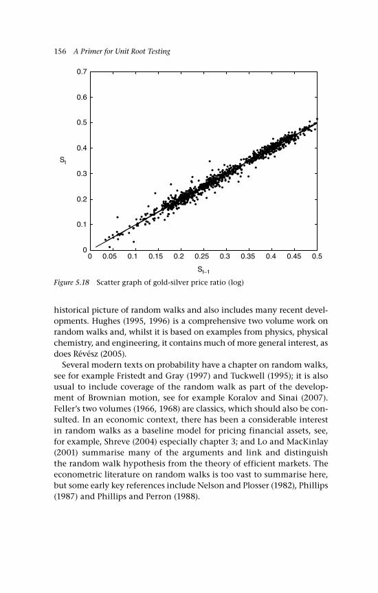
156 A Primer for Unit Root Testing
historical picture of random walks and also includes many recent devel-opments. Hughes (1995, 1996) is a comprehensive two volume work on random walks and, whilst it is based on examples from physics, physical chemistry, and engineering, it contains much of more general interest, as does Révész (2005).
Several modern texts on probability have a chapter on random walks, see for example Fristedt and Gray (1997) and Tuckwell (1995); it is also usual to include coverage of the random walk as part of the develop-ment of Brownian motion, see for example Koralov and Sinai (2007). Feller’s two volumes (1966, 1968) are classics, which should also be con-sulted. In an economic context, there has been a considerable interest in random walks as a baseline model for pricing financial assets, see, for example, Shreve (2004) especially chapter 3; and Lo and MacKinlay (2001) summarise many of the arguments and link and distinguish the random walk hypothesis from the theory of efficient markets. The econometric literature on random walks is too vast to summarise here, but some early key references include Nelson and Plosser (1982), Phillips (1987) and Phillips and Perron (1988).
0 0.05 0.1 0.15 0.2 0.25 0.3 0.35 0.4 0.45 0.50
0.1
0.2
0.3
0.4
0.5
0.6
0.7
St
St−1
Figure 5.18 Scatter graph of gold-silver price ratio (log)
An Introduction to Random Walks 157
Questions
Q5.1 Peter visits the gambling casino for the second time having won handsomely the night before. He is betting on whether the ball on a roulette wheel lands red or black, winning or losing an equal amount. After 20 games his cumulative winnings have not been neg-ative and, therefore, he argues that his winning streak is continuing and that he should continue to bet because luck must be on his side! Is he right?
On the other hand Peter argues that if he had only spent half the time in a winning position, he would not have felt so lucky and would have stopped betting. Is he right?
A5.1 First, consider the probability that his tally would never be nega-tive after 20 games. His tally St is a symmetric binomial random walk, with the probability that St is always positive given by (5.5) with t = 2n. For t = 20, this is:
P S tC
t( : , , ) .≥ = =
=0 1 202
0 176220 1020
A probability of 0.1762 that Peter’s tally did not go negative in 20 plays, that is about a one-in-six chance, so although Peter might con-sider himself lucky, the probability is perhaps larger than he thought. As to whether he has a lucky streak, the random walk has independent increments, so the probability of winning on the next gamble is unaf-fected by his previous good fortune: it is still ½.
The next question is what is the probability of Peter spending half of his time in a winning position in 20 games? To answer this, we use (5.8a), to obtain the probability of spending exactly = ½ of his time on the positive side. Set 2k = 10, 2n = 20, then:
PC
( ) .12
10 5102
20 0606=
=
Note that the approximation in (5.8b) gives the probability as 0.0637. Thus, the probability of = ½ is just over 6%, which reflects the general pattern shown in Figure 5.4 that P() is at a minimum where = ½, and is symmetric about this point, increasing towards the two extremes = 0 and = 1. So as to Peter’s judgement, the least likely outcome was
158 A Primer for Unit Root Testing
that he would spend exactly half his time on the positive side, but if he did, again it would not affect the probability of winning on the next gamble.
Q5.2 Let S y yt jj
t
j y==∑ 1
20, ~ ( , ) , show the following and establish the general pattern for cov(St, St+1):
cov( , ) cov( , )
cov( , ) cov( , ) cov(
S S y y
S S y y
y
y
1 22
1 2
2 32
1 2
2
2 2
= +
= + +
yy y y y1 3 2 3, ) cov( , )+
Also show that cov( , ) var( ) cov( )S S S y yt t t i ti
t
+ +== + ∑1 11
.
A5.2 Working through the examples remembering that E(yj) = 0 and expectation is a linear operator, then the following sequence is established:
cov( , ) cov( , )
[ ( )]
cov( )
cov( ,
S S y y y
E y y y
y y
Sy
1 2 1 1 2
1 1 2
21 2
2
= += +
= +
SS y y y y y
E y E y E y y E y y E3 1 2 1 2 3
12
22
1 2 1 32
) cov( , )
( ) ( ) ( ) ( ) (
= + + +
= + + + + yy y
y y y y y y
S S yy
2 3
21 2 1 3 2 3
3 4
2 2
)
cov( ) cov( ) cov( )
cov( , ) cov(
= + + +
=
11 2 3 1 2 3 4
21 2 1 3 2 3 13 2 2 2
+ + + + +
= + + + +
y y y y y y
E y y E y y E y y E yy
, )
( ) ( ) ( ) ( yy E y y
E y y
y y y yy i jj ii i
4 2 4
3 4
2
1
3
1
2
43 2
) ( )
( )
cov( ) cov( )
+
+
= + += += ∑∑
ii
y i jj ii iiS S y y y y
=
= += =
∑∑∑= + +
1
3
4 52
1
4
1
3
51
44 2cov( , ) cov( ) cov( ) ∑∑
In general:
cov( , ) cov( ) cov( )S S t y y y yt t y i jj i
t
i
t
i ti
t
+ = +=
−+=
= + +∑∑12
11
1
112 ∑∑
∑= + +=var( ) cov( )S y yt i ti
t
11
The last result follows either on noting the relationship directly or
cov( , ) cov( , )
var( ) cov( , )
var( )
S S S S y
S S y
S
t t t t t
t t t
t
+ +
+
= +
= +
= +
1 1
1
ccov( , )
var( ) cov( )
y y y
S y y
t t
t i ti
t
1 1
11
+ +
= ++
+=∑
An Introduction to Random Walks 159
Q5.3 The time series of the ratio of the gold to silver price shows 32 changes of sign in 5,372 observations. Is this prima facie evidence of a random walk? Suppose that the variable of interest is the log of the ratio of the gold to silver price: how many changes of sign will there be in the log ratio series?
A5.3 In the case of Gaussian inputs, the expected number of sign changes is 0.6363 T , which is 46.4 for T = 5,372; whereas for bino-mial inputs, it is 0.7979 T = 58.5. In both cases, the actual number of changes is below the expected number, but it is on the right side to suggest that the data could be generated by a random walk process. A more formal test can be designed and this is the subject of Chapter 8, Section 8.5. As to the second part of the question, the number of times that a particular level is crossed is invariant to a continuous monotonic transformation. Intuitively, if the original series is subject to a monot-onic transformation then so is the level, so that the number of crossings in the transformed series is just the same as in the original series. This is useful if a random walk is suspected, but there is there is uncertainty as to whether it is in the original series or some (monotonic) transforma-tion of the series.
160
6Brownian Motion: Basic Concepts
160
Introduction
Brownian motion is a key concept in economics in two respects. It underlies an important part of stochastic finance, which includes the pricing of risky assets, such as stock prices, bonds and exchange rates. For example a central model for the price of a risky asset is that of geometric Brownian motion (see Chapter 7). It also plays a key role in econometrics, especially in the distribution theory underlying test statistics for a unit root. For example, the limiting distribution of the familiar Dickey-Fuller pseudo-t test for a unit root is a functional of Brownian motion.
In both cases, but in different contexts, it is possible to relate the importance of Brownian motion to the limit of a random walk process in which the steps of the random walk become smaller and smaller. The process can be viewed in the limit as occurring in continuous time; the stochastic difference equation becomes a stochastic differential equation and the random walk generates a sample path of Brownian motion. Solving the stochastic differential equation requires use of the Itô calculus. This chapter outlines the key concept of Brownian motion, whereas the next chapter is a non-technical introduction to Itô calcu-lus. Together these chapters provide some familiarity with the language that is used in more advanced texts and especially in the asymptotic distribution theory for unit root tests. A number of references to more advanced works are provided at the end of the chapter for the interested reader.
This chapter is organised as follows. Section 6.1 introduces the definition of Brownian motion and Section 6.2, picking up on Chapter 5, links this to the limit of a random walk; Section 6.3 outlines the function space
Brownian Motion: Basic Concepts 161
on which BM is defined and Section 6.4 summarises some key proper-ties of Brownian motion. Brownian bridges occur quite frequently in the distribution theory of unit root tests and these are introduced in Section 6.5. The central limit theorem and the continuous mapping theorem, as they apply to functional spaces, are two essential tools for the analysis of unit root test statistics and these are outlined in Section 6.6. The use of these theorems is illustrated in Chapter 8, to obtain the limiting distributions of two widely used test statistics for a unit root due to Dickey and Fuller (see Fuller, 1976).
6.1 Definition of Brownian motion
The concept of Brownian motion is critical to the development of many scientific disciplines, including biology, engineering, physics, meteorol-ogy and chemistry, as well as economics. The stochastic process W(t) defined in continuous time is said to be a Brownian motion (BM) proc-ess if the following three conditions are met:
BM1: W(0) = 0.BM2: the increments are independent and stationary over time.BM3: W(t) ~ N(0, t2); that is W(t) is normally distributed with mean
zero and variance t2.
This process is also referred to as a Weiner process (Weiner, 1923). It is a standard Brownian motion process if 2 = 1, when it will be denoted B(t). If 2 ≠ 1 and W(0) = 0, then B(t) = W(t)/ converts the process to have a unit variance and become standard BM. If W(0) = µ ≠ 0, and 2 ≠ 1, then B(t) = [W(t) – ]/ is standard BM ⇒ W(t) = µ + B(t). A trended BM is obtained if W(t) = βt + B(t), so that B(t) = [W(t) – t]/ is stand-ard BM.
A word on notation is appropriate at this stage: a reasonably stand-ard notation in this area is to denote time in general by letters of the alphabet, for example s and t and, thus, to refer to, say, W(s) and W(t) as Brownian motion at times s and t. If the context does not require reference to more than two or three distinct times, then this notation will suffice. Otherwise, if a time sequence of general length is defined, the convention is to use a subscript notation on t, otherwise too many letters are required; thus, t1, t2, ... tn is an increasing sequence of the time index, for example corresponding to the Brownian motions W(t1), W(t2) and W(tn). As time is here a continuous index, there is no requirement that any of these indices are integers.

162 A Primer for Unit Root Testing
What are the characteristics of Brownian motion that make it attrac-tive as a model of physical and human behaviour? BM provides a mathematical model of the diffusion, or motion over time, of erratic particles; consider two examples, the first being Robert Brown’s origi-nal observation in 1827 that pollen grains suspended in water exhib-ited a ceaseless erratic motion; being bombarded by water molecules, the pollen seemed to be the subject of a myriad of chance movements. A similar phenomenon can be observed with smoke particles collid-ing with air molecules. In both examples, the trajectory of the particle over any small period is spiky and seemingly chaotic, but observed over a longer period the particle traces out a smoother path that has local trends.
In an economic context, it is evident that the behaviour of stock prices over time, particularly very short periods of time, can be quite erratic – or noisy; however, over a longer period, a direction is imparted to the level of the series. The point then is how to model this process: what is required is a model in which at any one point, or small interval, movement, as captured by the ‘increments’, is erratic and seemingly without structure, whereas over a longer period, the individual erratic movements are slight relative to the whole path. Hence, a key element of BM is the way that the erratic increments are built up into the level of the series. Whilst BM specifies normal increments, it can be generalised to increments from other distributions as might be appropriate for some financial asset prices, whose distributions exhibit much greater kurtosis than would be found in a normal distribution.
6.2 Brownian motion as the limit of a random walk
It is helpful to revisit the random walk of Chapter 5, and view Brownian motion as the limiting version of this process, where the limit is taken as the time interval between steps in the random walk is made smaller and smaller. Thus, in the limit the random walk becomes a continuous process.
6.2.1 Generating sample paths of BM
As an artificial, but helpful, device consider the length of the walk, T, as fixed and view this length as being divided into ‘small’ steps, where there are N of these relative time divisions, so that ∆t = T/N. By allowing N to increase, these time divisions become smaller, approaching 0 and, thus, in the limit, with T fixed, as N → ∞, the random walk process becomes continuous. In such a case,
Brownian Motion: Basic Concepts 163
there is no loss in fixing the length of walk as the unit interval, so that T = 1, and, therefore, ∆t = 1/N. The time index is not a set of integers, so we adopt the notation (referred to above), that the time index is t1 < t2 < ... < tN; in general, tj ≡ tj – tj–1, but we may, for convenience, set ∆t equal to a constant so that tj = tj–1 + t. Having established the limit of the random walk, which turns out to be Brownian motion, the method can also be used to establish the limit of some impor-tant partial sum processes, which are scaled random walks, arising in econometric theory.
The other parameter in the random walk is the size of each step, or win/loss amount in a gamble, which is taken to be S tt t= ( ) where t is distributed as iid(0, 2). We could alternatively base the random walk on the inputs yt = (–1, +1) and p = q = ½, which defines a symmet-ric binomial random walk, with the same limiting results see Equations (6.2) and (6.3) below, and see also Shreve (2004, section 3.2.5) and Iacus (2008, section 1.6.1). A question, see Q6.1 below, further explores this variant.
The variance of St is, (t)2 and if we return to the case where t = 1, that is time increments by one (whole) unit, then Var(St) = 2, which is as before. The random walk is now:
S S tt t tj j= +
−1( ) (6.1)
The variance of Stj, var(Stj
), will be needed, but we know this to be var(Stj) = tj
2; if 2 = 1, then tj2 = tj.
The limit of interest is obtained as N → ∞, with T fixed, such that:
S
NN t
t
D jj
⇒ ( , )0
(6.2)
This result follows by application of the standard central limit theo-rem, see Chapter 4, Section 4.2.3. Thus, scaled by N , the asymptotic (with N) partial sum process, or random walk, has a normal distribution with variance var(Stj
) = tj; therefore, dividing the scaled partial sum by tj results in a random variable, defined as Ztj
, which is distributed as N(0, 1). In summary:
ZS
t Nt
t
jDj
j≡ ⇒
N( , )0 1
(6.3)
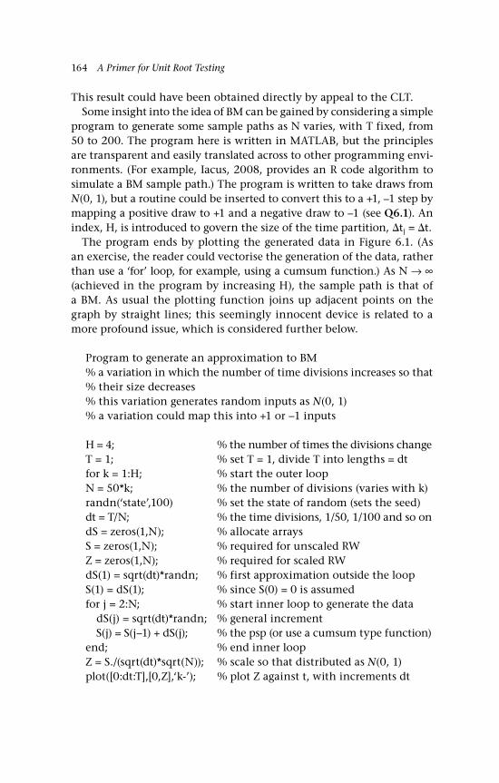
164 A Primer for Unit Root Testing
This result could have been obtained directly by appeal to the CLT.Some insight into the idea of BM can be gained by considering a simple
program to generate some sample paths as N varies, with T fixed, from 50 to 200. The program here is written in MATLAB, but the principles are transparent and easily translated across to other programming envi-ronments. (For example, Iacus, 2008, provides an R code algorithm to simulate a BM sample path.) The program is written to take draws from N(0, 1), but a routine could be inserted to convert this to a +1, –1 step by mapping a positive draw to +1 and a negative draw to –1 (see Q6.1). An index, H, is introduced to govern the size of the time partition, tj = t.
The program ends by plotting the generated data in Figure 6.1. (As an exercise, the reader could vectorise the generation of the data, rather than use a ‘for’ loop, for example, using a cumsum function.) As N → ∞ (achieved in the program by increasing H), the sample path is that of a BM. As usual the plotting function joins up adjacent points on the graph by straight lines; this seemingly innocent device is related to a more profound issue, which is considered further below.
Program to generate an approximation to BM% a variation in which the number of time divisions increases so that % their size decreases% this variation generates random inputs as N(0, 1)% a variation could map this into +1 or −1 inputs
H = 4; % the number of times the divisions changeT = 1; % set T = 1, divide T into lengths = dtfor k = 1:H; % start the outer loopN = 50*k; % the number of divisions (varies with k)randn(‘state’,100) % set the state of random (sets the seed)dt = T/N; % the time divisions, 1/50, 1/100 and so ondS = zeros(1,N); % allocate arraysS = zeros(1,N); % required for unscaled RWZ = zeros(1,N); % required for scaled RWdS(1) = sqrt(dt)*randn; % first approximation outside the loopS(1) = dS(1); % since S(0) = 0 is assumedfor j = 2:N; % start inner loop to generate the data dS(j) = sqrt(dt)*randn; % general increment S(j) = S(j−1) + dS(j); % the psp (or use a cumsum type function)end; % end inner loopZ = S./(sqrt(dt)*sqrt(N)); % scale so that distributed as N(0, 1)plot([0:dt:T],[0,Z],‘k-’); % plot Z against t, with increments dt

Brownian Motion: Basic Concepts 165
hold on; % plots all H figures on one graphpause ylabel(‘Z(t)’,‘FontSize’,14) title(‘Figure 6.1 Random walk approximation to BM’,‘FontSize’,14)end; % end outer loop % end of program
0 0.1 0.2 0.3 0.4 0.5 0.6 0.7 0.8 0.9 1−1.5
−1
−0.5
0
0.5
1
1.5
Z(t)
N = 50
N = 200
N = 150
N = 100
Figure 6.1 Random walk approximation to BM
6.3 The function spaces: C[0, 1] and D[0, 1]
In the previous section the random walk was viewed as taking place over the domain [0, 1] and the divisions in [0, 1], over which the random walk was evaluated, were then made smaller and smaller so that in the limit, the discretely realised random walk becomes continuous. The notation of continuous time was adopted with time index t1 < t2 < ... < tN.
A similar strategy, but with a different notational convention, is widely adopted in analysing unit root tests. It acknowledges the feature of economic time series data that they tend to be equally spaced. In this case T is variable and the domain is converted to [0, 1] by the creation of equally spaced divisions of length 1/T resulting in the series [0, 1/T, 2/T, ... , t/T, ... , 1]. The movement across the domain is indexed by r,
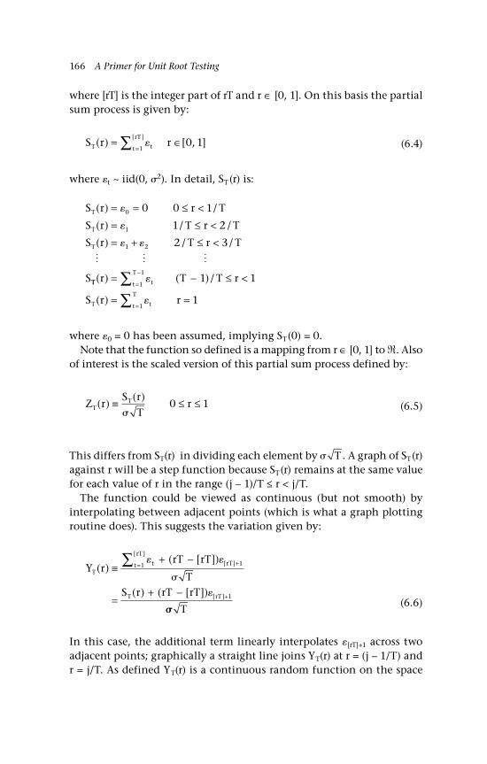
166 A Primer for Unit Root Testing
where [rT] is the integer part of rT and r ∈ [0, 1]. On this basis the partial sum process is given by:
S r rT tt
rT( ) [ , ]
[ ]= ∈
=∑ 1
0 1
(6.4)
where t ~ iid(0, 2). In detail, ST(r) is:
S r r T
S r T r T
S r T r T
S
T
T
T
( ) /
( ) / /
( ) / /
= = ≤ <
= ≤ <
= + ≤ <
0
1
1 2
0 0 1
1 2
2 3
TT tt
T
T tt
T
r T T r
S r r
( ) ( )/
( )
= − ≤ <
= ==
−
=
∑∑
1
1
1
1 1
1
where 0 = 0 has been assumed, implying ST (0) = 0.Note that the function so defined is a mapping from r ∈ [0, 1] to . Also
of interest is the scaled version of this partial sum process defined by:
Z rS r
TrT
T( )( )
≡ ≤ ≤
0 1
(6.5)
This differs from ST(r) in dividing each element by T . A graph of ST (r) against r will be a step function because ST (r) remains at the same value for each value of r in the range (j – 1)/T ≤ r < j/T.
The function could be viewed as continuous (but not smooth) by interpolating between adjacent points (which is what a graph plotting routine does). This suggests the variation given by:
Y rrT rT
TS r rT rT
Tt rTt
rT
T rT
( )( [ ])
( ) ( [ ])
[ ]
[ ]
[ ]
≡+ −
=+ −
+=
+
∑
11
1
T (6.6)
In this case, the additional term linearly interpolates [rT]+1 across two adjacent points; graphically a straight line joins YT(r) at r = (j – 1/T) and r = j/T. As defined YT(r) is a continuous random function on the space
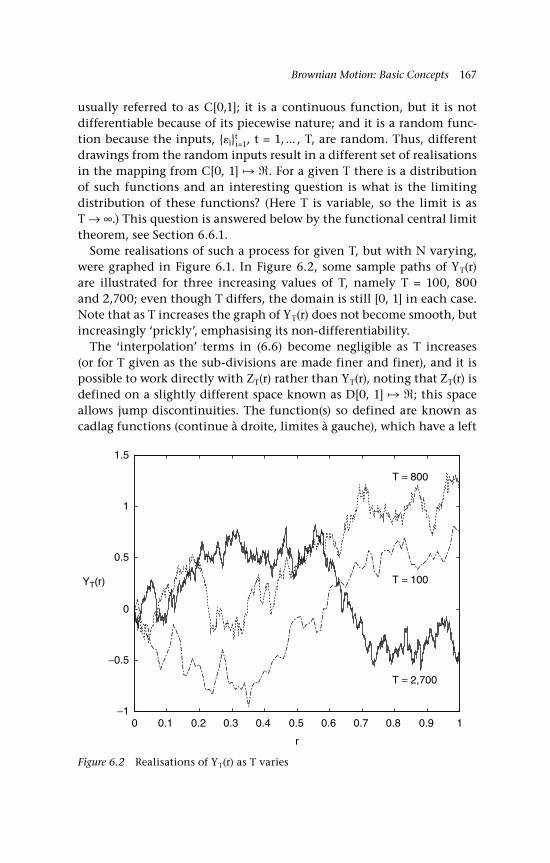
Brownian Motion: Basic Concepts 167
usually referred to as C[0,1]; it is a continuous function, but it is not differentiable because of its piecewise nature; and it is a random func-tion because the inputs, iti=1, t = 1, ... , T, are random. Thus, different drawings from the random inputs result in a different set of realisations in the mapping from C[0, 1] . For a given T there is a distribution of such functions and an interesting question is what is the limiting distribution of these functions? (Here T is variable, so the limit is as T → ∞.) This question is answered below by the functional central limit theorem, see Section 6.6.1.
Some realisations of such a process for given T, but with N varying, were graphed in Figure 6.1. In Figure 6.2, some sample paths of YT(r) are illustrated for three increasing values of T, namely T = 100, 800 and 2,700; even though T differs, the domain is still [0, 1] in each case. Note that as T increases the graph of YT(r) does not become smooth, but increasingly ‘prickly’, emphasising its non-differentiability.
The ‘interpolation’ terms in (6.6) become negligible as T increases (or for T given as the sub-divisions are made finer and finer), and it is possible to work directly with ZT(r) rather than YT(r), noting that ZT(r) is defined on a slightly different space known as D[0, 1] ; this space allows jump discontinuities. The function(s) so defined are known as cadlag functions (continue à droite, limites à gauche), which have a left
0 0.1 0.2 0.3 0.4 0.5 0.6 0.7 0.8 0.9 1−1
−0.5
0
0.5
1
1.5
r
T = 100
T = 800
T = 2,700
YT(r)
Figure 6.2 Realisations of YT(r) as T varies
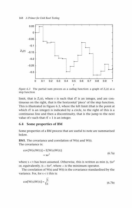
168 A Primer for Unit Root Testing
limit, that is ZT(r), where r is such that rT is an integer, and are con-tinuous on the right, that is the horizontal ‘piece’ of the step function. This is illustrated in Figure 6.3, where the left limit (that is the point at which rT is an integer) is indicated by a circle, to the right of this is a continuous line and then a discontinuity, that is the jump to the next value of r such that rT + 1 is an integer.
6.4 Some properties of BM
Some properties of a BM process that are useful to note are summarised below.
BM1. The covariance and correlation of W(s) and W(t).The covariance is:
cov[ ( ) ( )] ( ) ( )W s W t E W s W t
s
=
= 2
(6.7a)
where s < t has been assumed. Otherwise, this is written as min (s, t)2 or, equivalently, (s ∧ t)2, where ∧ is the minimum operator.
The correlation of W(s) and W(t) is the covariance standardised by the variance. For, for s < t this is:
cor W s W tst
[ ( ) ( )] = (6.7b)
0 0.1 0.2 0.3 0.4 0.5 0.6 0.7 0.8 0.9 1
−0.3
−0.25
−0.2
−0.15
−0.1
−0.05
0
0.05
r
ZT(r)
Figure 6.3 The partial sum process as a cadlag function: a graph of ZT(r) as a step function
Brownian Motion: Basic Concepts 169
BM2. Multivariate normality of the increments and the levels.
Let 0 = t0 < t1 < t2 < ... < tN = t, then the BM for tj is denoted W(tj) and the increments over these intervals are given by W(tj) ≡ W(tj) – W(tj–1). Let W and W be defined by the vector collections of these quantities:
W W t W t W t
W W t W t W t W t W tN
N
≡ ( )≡ − − −
( ), ( ), , ( ) ’
( ) , ( ) ( ), , ( ) (1 2
1 2 10 NN−( )1) ’
Then W has a multivariate normal distribution with covariance matrix E[WW], where the i-th diagonal element is ti
2 and ij-th off-diagonal element is min (ti, tj)2; the covariance matrix of E[WW] has i-th diagonal element equal to (ti – ti–1)2 and all off-diagonal ele-ments are zero; the latter follows as the increments of a BM process are independent.
BM3. A BM process is a martingale.
E[W(tj) |F0ti)] = W(ti) for all i ≤ j, where the filtration F0
ti = (W(ti), W(tt–1) ... W(t0)); and ( ) ( )W t W tj j j
N− − =1 1 forms a martingale difference sequence (MDS), see Q6.2 and Chapter 3, Section 3.5.1 for the definition of a martingale and an MDS.
BM4. A BM process has the Markov property (see Chapter 3, Section 3.5.2).
That is: E f W t g W tjt
ii[ ( ( )) | )] ( ( ))F0 = , where f(.) and g(.) are Borel-measurable
functions; (for an elaboration of both the martingale and Markov prop-erties of BM, see, for example, Shreve, 2004; for the concept of Borel-measurable functions see Chapter 1).
BM5. Unbounded variation.
Brownian motion has unbounded variation along a sample path for p ≤ 2 and bounded variation for p > 2, where p is the order of variation. Consider p = 1 and p = 2, being first and second order (or quadratic), respectively, then BM5.i and BM5.ii elaborate on these properties.
BM5.i The limiting first order path-wise variation is infinite for BM.
Define the p-th order variation, p > 0, of the general function f(t) over the interval [t0, tN] as:
V t f t f tNp
j jj
N p( ) | ( ) ( ) |≡ −+=
−∑ 10
1
(6.8)
170 A Primer for Unit Root Testing
Next, take the limit so that the partition, denoted δ, of [t0, tN], becomes finer with the maximum subinterval → 0 as N → ∞, and define Vp(t) as:
V t V tpN N
p( ) lim ( )≡ →∞ (6.9)
Then the p-th order variation is bounded if:
sup Vp(t) <
First-order variation (p = 1) is a measure of the ‘up-and-down’ move-ment of a function ignoring the sign of the movement. If f(t) = W(t), that is f(.) is Brownian motion, then the path-wise variation is infinite; see, for example, Brzezniak and Zastawniak (1999, Theorem 6.5).
BM5.ii Quadratic path-wise variation increases without limit for BM.
The quadratic variation along a Brownian motion path (referred to as ‘pathwise’) is given by:
V t W t W tN j jj
N210
1 2( ) [ ( ) ( )]= −+=
−∑
(6.10)
V2N(t) is path-dependent as it refers to a particular sample path of
the realisations of a Brownian motion process. Taking the limit N → ∞, then V2(t) = t, so that the quadratic variation converges in mean square to t (see Shreve, 2004, Theorem 3.4.3, and Section 4.2.11), which implies that E[V2
N(t)] = t and var[V2N(t)] = 0. As t increases, the
quadratic variation increases uniformly with t. This stands in con-trast to continuous functions with continuous derivatives, which have quadratic variation of zero. The next property should, therefore, not be a surprise.
BM6. Neither Brownian motion nor its increments are differentiable.
Intuitively, this is due to the ‘spiky’ or erratic nature of the increments. Consider taking the limit of W(tj) as tj → 0, which is the derivative if the limit exists. We know from the properties of BM that W(tj) ~ N(0, tj
2), hence:
W t
tN
t
tN
tj
j
j
j j
( )~ ,
( ),0 0
2
2
2
=
(6.11)
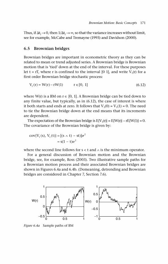
Brownian Motion: Basic Concepts 171
Thus, if tj → 0, then 1/tj → ∞, so that the variance increases without limit, see for example, McCabe and Tremayne (1993) and Davidson (2000).
6.5 Brownian bridges
Brownian bridges are important in econometric theory as they can be related to mean or trend adjusted series. A Brownian bridge is Brownian motion that is ‘tied’ down at the end of the interval. For these purposes let t = rT, where r is confined to the interval [0 1], and write V1(r) for a first order Brownian bridge stochastic process:
V r W r rW r1 1 0 1( ) ( ) ( ) [ , ]= − ∈ (6.12)
where W(r) is a BM on r ∈ [0, 1]. A Brownian bridge can be tied down to any finite value, but typically, as in (6.12), the case of interest is where it both starts and ends at zero. It follows that V1(0) = V1(1) = 0. The need to tie the Brownian bridge down at the end means that its increments are dependent.
The expectation of the Brownian bridge is EV1(r) = EW(r) – rEW(1) = 0. The covariance of the Brownian bridge is given by:
cov ( ), ( ) [( ) )]
( )
V s V t s t st
s t1 1
2
21
= ∧ −
= −
where the second line follows for s < t and ∧ is the minimum operator.For a general discussion of Brownian motion and the Brownian
bridge, see, for example, Ross (2003). Two illustrative sample paths for a Brownian motion process and their associated Brownian bridges are shown in Figures 6.4a and 6.4b. (Demeaning, detrending and Brownian bridges are considered in Chapter 7, Section 7.6).
Figure 6.4a Sample paths of BM
0 0.5 1−0.5
0
0.5
1
W(r)
0 0.5 1−1
−0.5
0
0.5
1
W(r)

172 A Primer for Unit Root Testing
6.6 Functional: Function of a function
Without explicit acknowledgement, a functional was introduced in Chapter 1, and this concept is of considerable importance in the econometrics of unit root testing. A functional is a function that has a function as its argument; it returns a number to a function argument. To understand what this means, recall that a function, y = f(x) takes the argument x and returns the value y. The domain of x denoted D is such that x ∈ D. For example, y = f(x) = x2 for x ∈ D = . If we then take this function as the argument of another function, wehave a functional, say F[f(.)]; for example, the functional F[.] given by
the definite integral F f x dxa
b[.] ( )= ∫ , so that with a = –1, b = +1 and y =
x2, then F x x dx[ ]2 2
1
12
3= =−
+
∫ and the functional assigns the number 2/3
as the functional outcome.
6.6.1 Functional central limit theorem, FCLT (invariance principle)
The FCLT is an important part of the ‘toolkit’ for the development of unit root test statistics. It deals with the extension of the standard CLT to functionals. We start with a particularly simple version, in which the stochastic inputs are t ∼ iid(0, 2), with 2 < ∞.
Consider the partial sum process and scaled partial sum process given, respectively, by:
S rT tt
rT( )
[ ]≡
=∑ 1
(6.18)
Z rS r
TTT( )( )
≡
(6.19)
Figure 6.4b Associated sample paths of Brownian bridge
0 0.5 1−1
−0.5
0
0.5
r0 0.5 1
−1
−0.5
0
0.5
1
r
tied down
tied down
V1(r) V1(r)
Brownian Motion: Basic Concepts 173
Then the FCLT states that:
Z r B rT D( ) ( )⇒ (6.20)
This is sometimes stated in slightly abbreviated form as ZT ⇒D B (or with a variant of the ⇒D notation). The FCLT (and CLT) is sometimes referred to as an invariance principle, IP, meaning that the convergence result is invariant to the distribution of the stochastic inputs that drive ST(r). Of course, some assumptions have to be made about these inputs, but these assumptions, discussed below, are relatively weak, and the FCLT is simply extended to cover such cases.
The notation ⇒D is used as in the case of conventional asymptotics where it indicates convergence in distribution; here it refers to the weak convergence of the probability measures, which is more encompassing than simply convergence in distribution, where the latter compares the distribution of one random variable with another. The nature of Brownian motion B(r) means that it is normally distributed for all r in the domain, its increments are normally distributed and it is jointly normally distributed for different values of r. The CLT is in this sense a by-product of the FCLT.
6.6.2 Continuous mapping theorem (applied to functional spaces), CMT
This is the extension of the CMT, which was introduced earlier, see sec-tion 4.2.2 Chapter 4, and it is often used in conjunction with the FCLT. This statement of the theorem is based on Davidson (1994, Theorem 26.13; 2000, Theorem 14.2.3) and is, in essence, the CMT applied to functionals rather than to functions.
Let g be a functional that maps D to the real line, expressed as g: D , which is continuous apart from a set of measure zero, expressed as Dg ∈ D, P(B ∈ Dg) = 0. Next, let the FCLT apply to ZT, such that ZT(r) ⇒D B(r), then g(ZT(r)) ⇒D g(B(r)). Important continuous func-tions for which this theorem is essential in unit root asymptotics are sums of ZT(r) and sums of squared ZT(r). (See Table 7.1 in Chapter 7, which summarises some frequently occurring functions in unit root econometrics.)
6.6.3 Discussion of conditions for the FCLT to hold and extensions
As in the case of the (standard) CLT and CMT, the FCLT and extended CMT are remarkable theorems that greatly simplify the derivation of
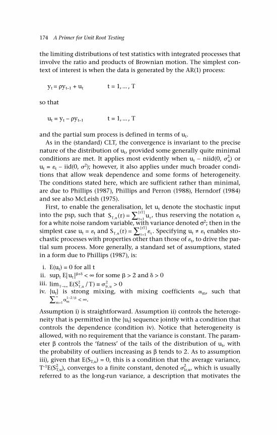
174 A Primer for Unit Root Testing
the limiting distributions of test statistics with integrated processes that involve the ratio and products of Brownian motion. The simplest con-text of interest is when the data is generated by the AR(1) process:
yt = ρyt–1 + ut t = 1, ... , T
so that
ut = yt – ρyt–1 t = 1, ... , T
and the partial sum process is defined in terms of ut.As in the (standard) CLT, the convergence is invariant to the precise
nature of the distribution of ut, provided some generally quite minimal conditions are met. It applies most evidently when ut ∼ niid(0, 2
u) or ut = t ∼ iid(0, 2); however, it also applies under much broader condi-tions that allow weak dependence and some forms of heterogeneity. The conditions stated here, which are sufficient rather than minimal, are due to Phillips (1987), Phillips and Perron (1988), Herndorf (1984) and see also McLeish (1975).
First, to enable the generalisation, let ut denote the stochastic input into the psp, such that S r uT u tt
rT
,
[ ]( ) =
=∑ 1, thus reserving the notation t
for a white noise random variable, with variance denoted σ2; then in the simplest case ut = t and S rT u tt
rT
,
[ ]( ) =
=∑ 1
. Specifying ut ≠ t enables sto-chastic processes with properties other than those of t, to drive the par-tial sum process. More generally, a standard set of assumptions, stated in a form due to Phillips (1987), is:
i. E(ut) = 0 for all t ii. supt E| ut |+ < ∞ for some > 2 and > 0iii. lim ( / ), ,T T u lr uE S T→∞ ≡ >2 2 0iv. ut is strong mixing, with mixing coefficients m, such that
mm
1 2
1
−=
∞∑ < ∞/ .
Assumption i) is straightforward. Assumption ii) controls the heteroge-neity that is permitted in the ut sequence jointly with a condition that controls the dependence (condition iv). Notice that heterogeneity is allowed, with no requirement that the variance is constant. The param-eter β controls the ‘fatness’ of the tails of the distribution of ut, with the probability of outliers increasing as β tends to 2. As to assumption iii), given that E(ST,u) = 0, this is a condition that the average variance, T–1E(S2
T,u), converges to a finite constant, denoted 2lr,u, which is usually
referred to as the long-run variance, a description that motivates the
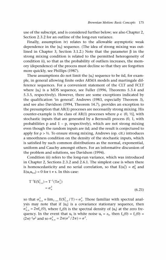
Brownian Motion: Basic Concepts 175
use of the subscript, and is considered further below; see also Chapter 2, Section 2.3.2 for an outline of the long-run variance.
Finally, assumption iv) relates to the allowable asymptotic weak dependence in the ut sequence. (The idea of strong mixing was out-lined in Chapter 3, Section 3.1.2.) Note that the parameter β in the strong mixing condition is related to the permitted heterogeneity of condition ii), so that as the probability of outliers increases, the mem-ory (dependence) of the process must decline so that they are forgotten more quickly, see Phillips (1987).
These assumptions do not limit the ut sequence to be iid, for exam-ple, in general allowing finite order ARMA models and martingale dif-ference sequences. For a convenient statement of the CLT and FCLT where ut is a MDS sequence, see Fuller (1996, Theorems 5.3.4 and 5.3.5, respectively). However, there are some exceptions indicated by the qualification ‘in general’. Andrews (1983, especially Theorem 3), and see also Davidson (1994, Theorem 14.7), provides an exception to the presumption that AR(1) processes are necessarily strong mixing. His counter-example is the class of AR(1) processes where ρ ∈ (0, ½], with stochastic inputs that are generated by a Bernoulli process (0, 1, with probabilities p and 1 – p, respectively), which are not strong mixing even though the random inputs are iid; and the result is conjectured to apply for ρ > ½. To ensure strong mixing, Andrews (op. cit.) introduces a smoothness condition on the density of the stochastic inputs, which is satisfied by such common distributions as the normal, exponential, uniform and Cauchy amongst others. For an informative discussion of the problem and solutions, see Davidson (1994).
Condition iii) refers to the long-run variance, which was introduced in Chapter 2, Sections 2.3.2 and 2.6.1. The simplest case is when there is homoscedasticity and no serial correlation, so that E(u2
t) = σ2u and
E(utut+s) = 0 for t ≠ s. In this case:
T E S T TT u u
u
− −=
=
1 2 1 2
2
( ) ( ),
(6.21)
so that lr u T T u uE S T, ,lim ( / )2 2 2≡ =→∞ . Those familiar with spectral anal-ysis may note that if ut is a covariance stationary sequence, then lr u uf, ( )2 2 0= , where fu(0) is the spectral density of ut at the zero fre-quency. In the event that ut is white noise ut = t, then fu(0) = f(0) = (2)–12 and so lr u, ( / )2 2 22 2= = .
176 A Primer for Unit Root Testing
In the case that 21r,u ≠ 2, with 0 < 2
lr,u < ∞, then the partial sum proc-ess is normalised using 2
1r,u rather than . The invariance principle is restated as follows. Let ST,u(r) and ZT(r) be defined by:
S r uT u tt
rT
,
[ ]( ) ≡
=∑ 1 (6.22)
Z rS r
TTT u
lr u
( )( ),
,
≡
(6.23)
where ut satisfies the conditions i) to iv) above, then, as before, but with these redefinitions:
Z r B rT D( ) ( )⇒ (6.24)
The conditions i) – iv) are not the only way to approach the characteri-sation of permissible heterogeneity and dependence in the ut sequence. The generality of the FCLT to processes that generate weakly dependent and heterogeneous errors has been studied by a number of authors; for different approaches see, for example, Wooldridge and White (1988), Phillips and Solo (1992), Andrews and Pollard (1994), Davidson (1994), de Jong (1997) and de Jong and Davidson (2000a, b).
Another way of approaching the invariance principle is to seek the normalising sequence aT for ST(r) such that:
Z rS ra
B rTT
TD( )
( )( )= ⇒
(6.25)
Then the cases so far correspond to aT = T and a TT lr u= , , respec-tively. In these cases ut is said to lie in the domain of normal attraction (DNA) of the normal law. That is despite heterogeneity, non-normality and weak dependence, ZT(r) acts, in the limit, as if it was normal. A case where this does not occur is when the variances of the elements of ut are infinite, as when the ut are drawn from the Cauchy distribution; even so ST(r) can be normalised so that it does converge, but to a Levy motion rather than a Brownian motion. These results have been generalised to other distributions. Let ut belong to the domain of attraction (DA) of a stable law with index α ∈ (0, 2), then the norming sequence is aT = T1/L(T), where L(T) is a slowly varying function. If ut belongs to the domain of normal attraction, then the norming sequence simplifies to a TT lr u= , , see Chan and Tran (1989) and Kourogenis and Pittis (2008).
Brownian Motion: Basic Concepts 177
6.7 Concluding remarks and references
Whilst it is possible to understand the general principles of unit root testing without reference to Brownian motion, for example the familiar DF pseudo-t test is just a t test, but with a non-standard distribution, some knowledge is essential for the asymptotic distribution theory. An understanding of Brownian motion also serves to emphasise the link with random walks and extensions, such as when the stochastic inputs are no longer Gaussian.
As noted in the previous chapter, most modern texts on probability theory include a section on Brownian motion and the references cited there will also be useful for BM; Fristedt and Gray (1997) is particularly good reference in this respect. Mikosch (1998) and Iacus (2008) are use-ful introductory references on Brownian motion, geometric Brownian motion and Brownian bridges, with the latter including program code in R. The monograph by Hida (1980) is devoted to Brownian motion. Shreve (2004) places the development of Brownian motion in the con-text of modelling the prices of financial assets. For an econometric per-spective, at a more advanced level, see Davidson (1994) and Hamilton (1994).
Questions
Q6.1 Rewrite the program in Section 6.2 to generate an approximation to BM from a symmetric binomial random walk.
AQ6.1 This variation requires that the partial sum process is defined as:
S S t yt t tj j= +
−1( )
where yt = (–1, + 1) with p = q = ½, hence 2y = 1. A program to gener-
ate the resulting approximation to BM follows for N = 100, ... , 800. The resulting output is shown in Figure Q6.1; note that the path is ‘spikier’ than when the inputs are N(0, 1), but that as the time divisions become smaller, the sample paths look very similar.
Program to generate an approximation to BM, via a symmetric binomial random walk
% the number of time divisions increases so that their size decreases% this variation generates random inputs as +1 or −1
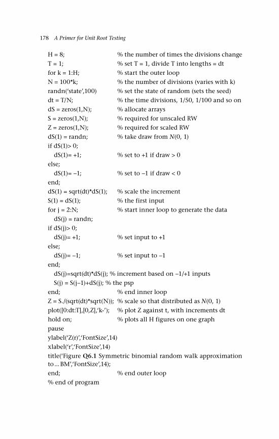
178 A Primer for Unit Root Testing
H = 8; % the number of times the divisions change
T = 1; % set T = 1, divide T into lengths = dt
for k = 1:H; % start the outer loop
N = 100*k; % the number of divisions (varies with k)
randn(‘state’,100) % set the state of random (sets the seed)
dt = T/N; % the time divisions, 1/50, 1/100 and so on
dS = zeros(1,N); % allocate arrays
S = zeros(1,N); % required for unscaled RW
Z = zeros(1,N); % required for scaled RW
dS(1) = randn; % take draw from N(0, 1)
if dS(1)> 0;
dS(1)= +1; % set to +1 if draw > 0
else;
dS(1)= −1; % set to −1 if draw < 0
end;
dS(1) = sqrt(dt)*dS(1); % scale the increment
S(1) = dS(1); % the first input
for j = 2:N; % start inner loop to generate the data
dS(j) = randn;
if dS(j)> 0;
dS(j)= +1; % set input to +1
else;
dS(j)= −1; % set input to −1
end;
dS(j)=sqrt(dt)*dS(j); % increment based on −1/+1 inputs
S(j) = S(j−1)+dS(j); % the psp
end; % end inner loop
Z = S./(sqrt(dt)*sqrt(N)); % scale so that distributed as N(0, 1)
plot([0:dt:T],[0,Z],‘k-’); % plot Z against t, with increments dt
hold on; % plots all H figures on one graph
pause
ylabel(‘Z(r)’,‘FontSize’,14)
xlabel(‘r’,‘FontSize’,14)
title(‘Figure Q6.1 Symmetric binomial random walk approximation to ... BM’,‘FontSize’,14);
end; % end outer loop
% end of program

Brownian Motion: Basic Concepts 179
The binomial inputs could also be generated via the uniform distribu-tion, see Iacus (2008, Section 1.6.1).
Q6.2 Show that the covariance between W(s) and W(r) for s < r is s2.
A6.2 First add and subtract W(s) to W(r) in the second term of the covariance:
cov[W(s), W(r)] = cov[W(s), (W(s) + W(r) – W(s)] = cov[W(s)W(s) + W(s)(W(r) – W(s))] = cov[W(s)W(s)] = var[W(s)] = s2
The result uses (2nd to 3rd line) the increment W(r) – W(s) is inde-pendent of W(s) and (4th to 5th line) the variance of W(s) is sσ2 or s if W(s) ≡ B(s).
Q6.3 Prove that a BM process is a martingale and that W(tj) – W(tj–1)
nj=1 forms a martingale difference sequence.
A6.3 If BM is a martingale it must satisfy E[W(t)|Fs0] = W(s) for s < t,
where Fs0 = W(u): u s. To show this, first add and subtract
Figure Q6.1 Symmetric binomial random walk approximation to BM
0 0.1 0.2 0.3 0.4 0.5 0.6 0.7 0.8 0.9 1−0.5
0
0.5
1
1.5
2
2.5
Z(r)
r
approximations to BMN = 100, ..., 800; ∆t = 1/N
N = 100
N = 800
180 A Primer for Unit Root Testing
W(s) within the expectation:
E W t E W t W s W s
E W t W s E W
s s
s
[ ( ) | ] [ ( ) ( ) ( ) | ]
[ ( ) ( ) | ] [
F F
F0 0
0
= − +
= − + (( ) | ]
[ ( ) | ]
( )
t
E W s
W s
s
s
F
F0
0==
where E[W(t) – W(s) | Fs0 ] because the increment W(t) – W(s) is independ-
ent of Fs0; E[W(s) | Fs
0] = W(s) because Fs0 includes W(s), so it is known at s.
It then follows that the sequence of differences, W(t) – W(s), each being a difference of a martingale, is a martingale difference sequence.
7Brownian Motion: Differentiation and Integration
181
Introduction
It was noted in Chapter 6 that Brownian motion is not differentiable along its path, that is with respect to t, see property BM6. However, even just a passing familiarity with the literature on random walks and unit root tests will have alerted the reader to the use of notation that corresponds to derivatives and integrals. In particular, the limiting dis-tributions of various unit root test statistics invariably involve integrals of Brownian motion. Given that these are not conventional integrals, what meaning is to be attributed to them? This chapter is a brief intro-duction to this topic, starting by a contrast with the nonstochastic case. As usual, further references are given at the end of the chapter.
This chapter is organised as follows. Section 7.1 comprises a brief review of integration in the nonstochastic case; the concept of integra-tion is extended to the stochastic case in Section 7.2, with the Itô for-mula and corrections outlined in Section 7.3. Some particular examples of stochastic differential equations, namely the Ornstein-Uhlenbeck process and geometric Brownian motion are introduced in Sections 7.4 and 7.5, respectively. Section 7.6 is concerned with the frequently occur-ring and important case where some form of detrending is first applied to a time series. Section 7.7 provides a tabular summary of some results involving functional of Brownian motion and a simulation example.
7.1 Nonstochastic processes
To start, consider a nonstochastic process that is a continuous function of time; for example, suppose the process evolves as dU(t) = U(t)dt, which is a first order differential equation. The path of U(t) can be obtained
182 A Primer for Unit Root Testing
by integrating dU(t) to obtain the solution U(t) = U(0)et, where U(0) is the initial condition. We can check that this does indeed satisfy the dif-ferential equation by differentiating U(t) with respect to t: thus, dU(t)/dt = U(0)et = U(t), as required.
Analogously, as Brownian motion is a continuous-time process, it might be tempting to write its derivative with respect to time as dW(t)/dt, the idea being to measure the change with respect to time along a Brownian motion path; however, as noted, this ‘derivative’ does not exist, although, of course, changes in the form of increments and dec-rements do exist. Neither does the ‘anti-derivative’ or integral, in the conventional sense, exist, so that the solution, W(t), cannot be obtained by conventional integration.
To make the point in another way, suppose the first order differential equation for U(t) is amended by adding a function of the increments of Brownian motion, say f(t)dW(t), where dW(t) is an increment on the Brownian motion path, so that dU(t) = U(t)dt + f(t)dW(t); it might be tempting to divide through by dt and let dt → 0; however, such an oper-ation is not valid given the non-differentiability of W(t). The first part of the solution is still valid, but in obtaining a complete solution a special meaning has to be attached to f s dW s
s
t( ) ( )
=∫ 0 other than that of the con-
ventional Reimann integral. As the path of a Brownian motion process is continuous and can be reconstructed from its increments/decrements and an initial condition, it must be possible to do something. The solu-tion to this problem is to use the Itô calculus, in which conventional (Reimann) integrals are replaced with Itô integrals. Reimann integrals are briefly reviewed in the next section as a precursor to the solution when deterministic functions are replaced by stochastic functions.
7.1.1 Reimann integral
It is helpful to first take a step back and consider an integral for a func-tion whose derivatives exist. In this case the conventional integral is a Reimann integral. Consider the function f(t) where (at least) df(t)/dt exists.
The integral is written f s dss
t( )
=∫ 0, where s is the variable of integration,
which can be viewed as the limit of the following discretisation:
I t f t t tRN
j j jj
N( ) ( )( )[ ]= −+=
−∑ 11
1
(7.1)
where 0 = t0 < t1 < t2 < ... < tn = t and f(t[j]) is the function f(t) evaluated in the interval tj to tj+1; for convenience assume that tj+1 ≡ (tj+1 – tj) = t, so
Brownian Motion: Differentiation and Integration 183
that the time increments are equal. Provided that the limit converges, the Reimann integral, IR(t), is obtained as N → ∞, so that the overall interval (0, t) is split into smaller and smaller parts such that t → 0. Each small interval is multiplied by the value of the function f(t) for a value of t in the interval tj+1; the resulting areas are then summed over all the disjoint partitions of the overall interval. In summary:
I t I tR N RN( ) lim ( )≡ →∞
(7.2)
We will often be interested in the integral over 0 = t0 < ... < tn = 1, in which case the Reimann integral is f s ds
s( )
=∫ 0
1
.
Example 7.1: Revision of some simple Reimann indefinite and definite integrals
By way of revision, consider the simple polynomial function y = f(t) = atb, b ≠ –1, with derivative ft %y / %t = abtb–1; then the indefinite integral is ftdt = (ab)tb–1dt. Often we are interested in the reverse procedure, that is given the indefinite integral what is y = f(t)? In this case, the solution is easy to obtain if we write xdx and note that β = b – 1 and α = ab, imply b = β + 1 and a = /b; for example, 4t3dt implies b = 3 + 1 = 4 and a = 4/4 = 1, so that y = t4 and, to check, ft = 4t3, as required. However, there is an element of non-uniqueness in this solution, because y = t4 + C, for C ≠ 0, results in the same derivative as for C = 0; hence, we should write ftdt = f(t) + C, where C is referred to as the constant of integra-tion. The definite integral corresponds to setting an upper and a lower limit to the range of integration, f dt ttg
h
gh∫ = 4 ] , where h ≥ g; for example,
4 1 0 13
0
1 401 4t dt t∫ = = − =] ( ) ( ) . ♦
7.1.2 Reimann-Stieltjes integral
An extension of the integration problem can be formulated by introduc-ing a continuous function of t, say, g(t), as the function of integration, rather than t itself. The problem is to integrate the function f(t), the integrand, with respect to the function g(t), the integrator. This leads to the Reimann-Stieltjes integral, where IN
R(t) is replaced by:
I t f t g t g tRSN
j j jj
N( ) ( )[ ( ) ( )][ ]= −+=
−∑ 11
1
(7.3)
184 A Primer for Unit Root Testing
This corresponds to the Reimann integral when g(t) = t, so that g(tj+1) = tj+1, but in the case of the Reimann-Stieltjes (RS) integral, each f(t[j]) is weighted by g(tj+1). In summary:
I t I tRS N RSN( ) lim ( )≡ →∞ (7.4)
The typical notation for the RS integral is f s dg ss
t( ) ( )
=∫ 0. As the functions
are deterministic, if the limit exists it is an element of the real line and the definite integral is a number, not a function.
The function g(t) may have jump discontinuities, but if it has bounded variation, then the RS integral will exist. If g(t) is everywhere differenti-able and the derivative gt ≡ %g(t)/%t is continuous, then the RS integral
f s dg ss
t( ) ( )
=∫ 0 coincides with the simple Reimann construction f s g dsts
t( )
=∫ 0;
but continuity of g(t) is not sufficient to ensure this, rather absolute continuity is required (see end of chapter glossary).
Bounded variation of g(t) is a sufficient condition for existence of the RS integral; however, Mikosch (1998) gives a more general sufficient condi-tion that is close to necessity. We cite one of his results here, see (Mikosch, op. cit., pp. 94–5), which uses the following sufficient conditions.
The functions f(t) and g(t) do not have discontinuities at the same 1. point of t ∈ [0, 1];f(t) and g(t) have bounded p-variation and q-variation, respectively, 2. where p–1 + q–1 > 1 for p > 0 and q > 0. (For the definition of p-th order variation see BM5.)
The RS integral does exist for some combinations of f(t) and g(t) when g(t) is replaced by Brownian motion, W(t). Let the function f(t) be a deterministic function of t or the sample path of a stochastic process on t ∈ [0, 1], 0 = t0 < ... < tn = 1; where f(t) is differentiable with a bounded derivative on [0, 1], for example f(t) = sin(t) or f(t) = tp; and W(s) is a Brownian motion on the same space. If conditions 1 and 2 are satisfied, then the following RS integral exists for every BM sample path:
I t f s dW sRS s( ) ( ) ( )≡
=∫ 0
1
(7.5)
See Mikosch (op. cit., p. 95). For example, I t sdW sRS s( ) ( )=
=∫ 0
1 exists in the
RS sense. However, this does not mean that the RS integral exists for general integrands; for example, the integral W s dW s
s( ) ( )
=∫ 0
1, which is
of particular interest in an econometric context, does not exist in the
Brownian Motion: Differentiation and Integration 185
RS sense; in this case, f(t) = g(t) = W(t) and variation is bounded only for p > 2, so the test for condition 2 is now on p–1 + p–1 = 2p–1, but this is < 1 for p > 2. Further arguments show that the failure of this sufficient condition also implies failure of the integral to be defined in the RS sense (see Mikosch, op. cit.,).
In what sense, therefore, does an integral exist and do the rules of classical calculus still apply? The answer to the first question is yes, an integral exists, but it differs from the Reimann-Stieltjes integral; the answer to the second question is no, not in general. These matters are considered in the next section.
7.2 Integration for stochastic processes
When dealing with stochastic processes, the starting point for defining an integral looks similar to that for the RS integral, but it leads to a dif-ferent development. Consider the particular example where we would like to obtain the integral W s dW s
s
t( ) ( )
=∫ 0 and, as usual, W(t) is Brownian
motion and s is the variable of integration. Then we could start by anal-ogy with the Reimann-Stieltjes sum, so that:
W t W t W tj j jj
N( )( ( ) ( ))[ ] +=
−−∑ 11
1
(7.6)
where W(tj+1) – W(tj) is just an increment to Brownian motion, so it is unambiguously defined; the problem is with W(t[j]), the critical point being that, in contrast to when W(t) was a differentiable function of t, it now matters where t[j] is chosen in the subinterval tj to tj+1. Consider three possibilities:
t[j] = tj; t[j] = ½(tj + tj+1); t[j] = tj+1.
That is the beginning of the interval, the mid-point of the interval and the end of the interval. Taking the former results in the Itô integral and taking the second results in the Stratonovich integral, whereas the latter choice does not appear to be in general use.
The Itô integral is in widespread use, not least because of its impor-tance in finance, where t[j] = tj relates to an ‘opening’ position rather than the ‘closing’ position that relates to choosing t[j] = tj+1, see, for example, Shreve (2004, especially chapter 4). It also corresponds to the space of cadlag functions on C[0, 1] as illustrated in Figure 6.3, with the
186 A Primer for Unit Root Testing
step function starting at the ‘opening’ position. Making this choice, the sum of interest is:
I t W t W t W tIN
j j jj
N( ) ( )( ( ) ( ))= −+=
−∑ 11
1 (7.7)
Also letting N → ∞, so that the divisions become finer and finer, then:
I1(t) limN→ INI(t) (7.8)
which is the limit of INI(t) as N → ∞. To obtain the limiting expres-
sion, which will be the Itô integral, first consider INI(t). Write a typical
component of the sum as a(b – a), noting that this is identically equal to ½[(b2 – a2) – (b – a)2]. Using this identity, the sum can be expressed as:
W t W t W t
W t W t W
j j jj
N
j jj
N
( )( ( ) ( ))
( ) ( )
+=
−
+=
−
−
= − −
∑
∑
11
1
12 2
1
112
(( ) ( )t W tj jj
N
+=
−− ( )∑ 1
2
1
1
(7.9)
Next, note that the first sum is equal to W(tN)2 – W(t0)2 and the second is the quadratic variation in W(t), so that:
I t W t W t V tIN
N N( ) ( ) ( ) ( )= − −( )12
20
2 2 (7.10)
Finally, noting that W(t0) = W(0) = 0, by the definition of Brownian motion, and that the limit of V2
N(t) is V2(t) = t, see BM5.ii, then the Itô integral of W s dW s
s
t( ) ( )
=∫ 0 is:
I t I t
W t tI N I
N( ) lim ( )
( )
=
= −( )→∞
12
2 (7.11)
Note that this differs from the Reimann integral by a term 1–2t, that depends on the quadratic variation of Brownian motion, which is zero for nonstochastic functions.
To show that the integral is sensitive to the point at which the function is evaluated, note that if t[j] = tj+1 then the resulting integral gives ½(W(t)2 + t), whereas if t[j] = ½(tj + tj+1) then the Stratonovich integral results in ½W(t)2. Only in this last case does the inte-gral coincide with the classical result that if w(t) is a continuous

Brownian Motion: Differentiation and Integration 187
deterministic function (reserving W(t) in upper case for BM) then w s dw s w s w s ds w t w T
s
T
s
T T( ) ( ) ( )( / ) / ( ) / ( )
= =∫ ∫= ∂ ∂ = =0 0
2
01
21
2 , where ]T0 indicates
the limits of the definite integral and, by analogy with BM we assume that w(0) = 0.
A particular application of the Itô integral result occurs when the var-iable of integration is limited to the interval 0 ≤ r ≤ 1, and the integral is taken over the whole range, then I WI ( ) ( )1 1 11
22= −( ). Such an integral
is sometimes written in conventional notation; in this case it would be W s dW s
s( ) ( )
=∫ 0
1, but this only makes sense on the understanding that
the integral referred to is the Itô integral (or another form of stochastic integral).
Returning to the stochastic differential equation dU(t) = U(t)dt + f(t)dW(t), the meaning of this can now be framed in terms of well-defined integrals as:
U t U U s ds f s dW ss
t
s
t( ) ( ) ( ) ( ) ( )− = +
= =∫ ∫00 0
(7.12)
where the first integral is a conventional integral and the second is an Itô integral (or an Reimann integral depending on the properties of f(t)), both of which now have well-defined meanings.
7.3 Itô formula and corrections
7.3.1 Simple case
The result that I t W s dW s W t tI s
t( ) ( ) ( ) ( )= = −( )
=∫ 0
12
2 , where W(t) is Brownian motion, is one example of an Itô integral. It contains the additional term 1–2t relative to the nonstochastic case. This term is related to the Itô correction of the standard integral and, in general, the additional term can be obtained by means of the Itô formula, which is given in simple and then more complex forms below.
If f(t) = fW(t), so that there is no dependence on t apart from through W(t), with derivatives fw %f(.)/dW(.) and fww %2f(.)/%W(.)2, then the Itô formula (which is a simplified version of the more general case given below) is:
f T f f dt f dW tWW
T
W
T( ) ( ) ( )− = +∫ ∫0 1
2 0 0 (7.13)
The second term on the right-hand-side is present in a conventional integral but the first term, which is the Itô correction, is not. Note that
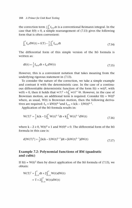
188 A Primer for Unit Root Testing
the correction term 12 0
f dtWW
T
∫ is a conventional Reimann integral. In the case that f(0) = 0, a simple rearrangement of (7.13) gives the following form that is often convenient:
f dW t f T f dtW
T
WW
T
0 0
12∫ ∫= −( ) ( ) (7.14)
The differential form of this simple version of the Itô formula is written as:
df t f dt f dW tWW W( ) ( )= +12 (7.15)
However, this is a convenient notation that takes meaning from the underlying rigorous statement in (7.13).
To consider the nature of the correction, we take a simple example and contrast it with the deterministic case. In the case of a continu-ous differentiable deterministic function of the form f(t) = w(t)k, with w(0) = 0, then it holds that w T k w t dtk kT
( ) ( )= −∫ 1
0. However, in the case of
Brownian motion, an additional term is required. Consider f(t) = W(t)k where, as usual, W(t) is Brownian motion, then the following deriva-tives are required: fw = kW(t)k–1and fww = k(k – 1)W(t)k–2.
Application of the Itô formula results in:
W T k k W t dt k W t dW tk kT kT( ) ( ) ( ) ( ) ( )= − +− −∫ ∫1
21 2
0
1
0
(7.16)
where k – 2 ≥ 0, W(t)0 ≡ 1 and W(0)k = 0. The differential form of the Itô formula in this case is:
d W T k k W t dt kW t dW tk k k ( ) [ ( ) ( ) ] [ ( ) ] ( )= − +− −12
1 2 1
(7.17)
Example 7.2: Polynomial functions of BM (quadratic and cubic)
If f(t) = W(t)2 then by direct application of the Itô formula of (7.13), we obtain:
W T dt W t dW t
T W t dW t
t
T
t
T
t
T
( ) ( ) ( )
( ) ( )
2
0 0
0
2
2
= +
= +
= =
=
∫ ∫∫
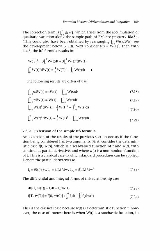
Brownian Motion: Differentiation and Integration 189
The correction term is dt Tt
T
=∫ =0
, which arises from the accumulation of quadratic variation along the sample path of BM, see property BM5.i. (This could also have been obtained by rearranging W s dW s
s
t( ) ( )
=∫ 0, see
the development below (7.11)). Next consider f(t) = W(T)3, then with k = 3, the Itô formula results in:
W T W t dt W t dW t
W t dW t W T W t
T T
T
( ) ( ) ( ) ( )
( ) ( ) ( ) ( )
3
0
2
0
2
0
3
0
3 3
13
= +
= −
∫ ∫
∫TT
dt∫ ♦
The following results are often of use:
sdW s tW t W s dss
t
s
t( ) ( ) ( )
= =∫ ∫= −0 0
(7.18)
rdW r W W r drr r
( ) ( ) ( )= =∫ ∫= −
0
1
0
11 (7.19)
W s dW s W t W s dss
t
s
t( ) ( ) ( ) ( )2
0
3
0
13= =∫ ∫= −
(7.20)
W r dW r W W r drr r
( ) ( ) ( ) ( )2
0
1 3
0
113
1= =∫ ∫= −
(7.21)
7.3.2 Extension of the simple Itô formula
An extension of the results of the previous section occurs if the func-tion being considered has two arguments. First, consider the determin-istic case f[t, w(t)], which is a real-valued function of t and w(t), with continuous partial derivatives and where w(t) is a non-random function of t. This is a classical case to which standard procedures can be applied. Denote the partial derivatives as:
f f t f f w f f wt w ww≡ ∂ ∂ ≡ ∂ ∂ ≡ ∂ ∂(.)/ , (.)/ , (.)/2 2 (7.22)
The differential and integral forms of this relationship are:
df t w t f dt f dw tt w[( , ( )] ( )= + (7.23)
f T w T f w f dt f dw tt
T
w
T[ , ( )] [ , ( )] ( )= + +∫ ∫0 0
0 0 (7.24)
This is the classical case because w(t) is a deterministic function t; how-ever, the case of interest here is when W(t) is a stochastic function, in

190 A Primer for Unit Root Testing
particular a Brownian motion process. In that case, the Itô formula, in integral and differential forms, is:
f T W T f W f f dt f dW tt WW W
TT[ , ( )] [ , ( )] ( ) = + + + ∫∫0 0 1
2 00
(7.25)
df t W t f f dt f dW tt WW W[( , ( )] ( ) = + +12
(7.26)
where the first integral in (7.25) is a Reimann integral (it is a function of t) and the second integral is an Itô integral (it is a function of W(t)). As in the simpler case of (7.13), comparing the two forms there is an additional term involving the second derivative, fww, of f[t, W(t)], which is the Itô correction; as noted, this arises because of the path-wise quad-ratic variation of Brownian motion.
Example 7.3: Application of the Itô formula
Consider the function f[t, W(t)] = tW(t)2, then ft = W(t)2, fw = 2tW(t) and fww = 2t. Hence, in integral and differential forms, the Itô formula results in:
f T W T W t t dt tW t dW t
d tW t W t t d
T T[ , ( )] ( ) ( ) ( )
( ) ( ( ) )
= + +
= +∫ ∫2
0 0
2
2
tt tW t dW t+ 2 ( ) ( ) ♦
Example 7.4: Application of the Itô formula to the exponential martingale
Let Y(t, W(t)) = ew(t)e–(1/2)t, which is a process known as an exponen-tial martingale (see Brzezniak and Zastawniak, 1999): obtain the inte-gral and differential forms, as in (7.25) and (7.26). First note that the required derivatives are:
f e e Y t W t
f e e Y t W t
tW t t
WW t t
= − = −
= =
−
−
12
12
1 2
1 2
( ) ( / )
( ) ( / )
( , ( ))
( , ( ))
ff e e Y t W tWWW t t= =−( ) ( / ) ( , ( ))1 2
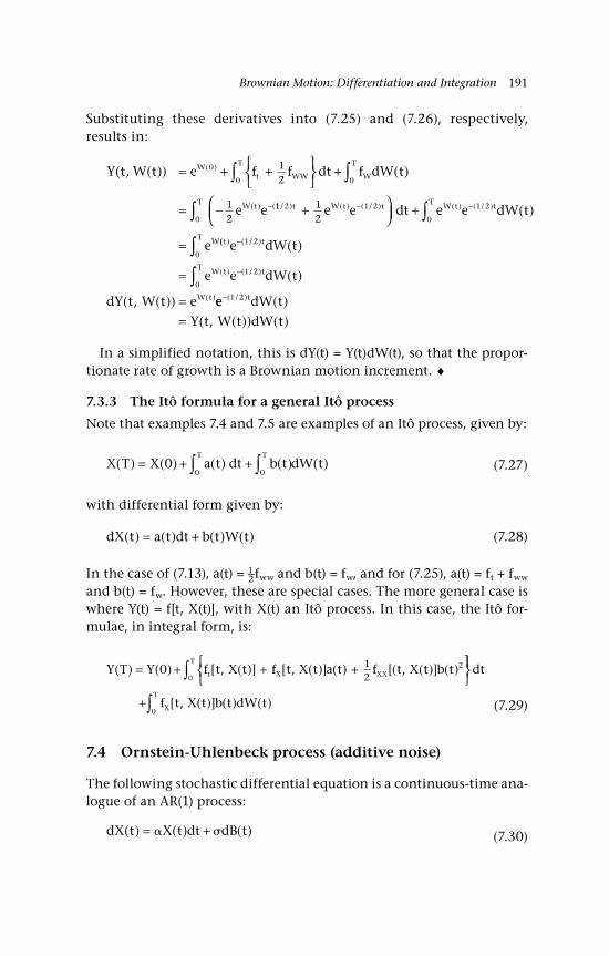
Brownian Motion: Differentiation and Integration 191
Substituting these derivatives into (7.25) and (7.26), respectively, results in:
Y t W t e f f dt f dW t
e e
Wt WW
T
W
T
W t
( , ( )) ( )( )
( ) (
= + +
+
= −
∫ ∫−
0
0 0
12
12
11 2 1 2
0
1 2
0
12
/ ) ( ) ( / ) ( ) ( / ) ( )t W t tT W t tT
W
e e dt e e dW t
e
+
+
=
− −∫ ∫(( ) ( / )
( ) ( / )
( )
( )
( )
( , ( ))
t tT
W t tT
W t
e dW t
e e dW t
dY t W t e
−
−
∫∫=
=
1 2
0
1 2
0
ee dW t
Y t W t dW t
t−
=
( / ) ( )
( , ( )) ( )
1 2
In a simplified notation, this is dY(t) = Y(t)dW(t), so that the propor-tionate rate of growth is a Brownian motion increment. ♦
7.3.3 The Itô formula for a general Itô process
Note that examples 7.4 and 7.5 are examples of an Itô process, given by:
X T X a t dt b t dW tT T
( ) ( ) ( ) ( ) ( )= + +∫ ∫00 0
(7.27)
with differential form given by:
dX t a t dt b t W t( ) ( ) ( ) ( )= + (7.28)
In the case of (7.13), a(t) = 1–2fww and b(t) = fw, and for (7.25), a(t) = ft + fww
and b(t) = fw. However, these are special cases. The more general case is where Y(t) = f[t, X(t)], with X(t) an Itô process. In this case, the Itô for-mulae, in integral form, is:
Y T Y f t X t f t X t a t f t X t b tt X XX( ) ( ) [ , ( )] [ , ( )] ( ) [( , ( )] ( )= + + +
0 12
2
+
∫
∫
dt
f t X t b t dW t
T
X
T
0
0[ , ( )] ( ) ( )
(7.29)
7.4 Ornstein-Uhlenbeck process (additive noise)
The following stochastic differential equation is a continuous-time ana-logue of an AR(1) process:
dX t X t dt dB t( ) ( ) ( )= + (7.30)
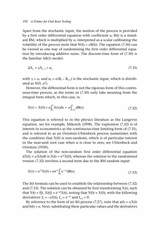
192 A Primer for Unit Root Testing
Apart from the stochastic input, the motion of the process is provided by a first order differential equation with coefficient ; B(t) is a stand-ard BM, which is multiplied by , interpreted as a scalar calibrating the volatility of the process (note that W(t) = B(t)). The equation (7.30) can be viewed as one way of randomising the first order differential equa-tion by introducing additive noise. The discrete-time form of (7.30) is the familiar AR(1) model:
X X ut t t= +− 1 (7.31)
with = , and ut = (Bt – Bt–1) is the stochastic input, which is distrib-uted as N(0, 2).
However, the differential form is not the rigorous form of this contin-uous-time process, as the terms in (7.30) only take meaning from the integral form which, in this case, is:
X t X X s ds dB st
s
t( ) ( ) ( ) ( )= + +∫ ∫ =
00 0
(7.32)
This equation is referred to in the physics literature as the Langevin equation, see for example, Mikosch (1998). The expression (7.32) is of interest in econometrics as the continuous-time limiting form of (7.31), and is referred to as an Ornstein-Uhlenbeck process (sometimes with the condition that X(0) is non-random), which is of particular interest in the near-unit root case when α is close to zero; see Uhlenbeck and Ornstein (1930).
The solution of the non-random first order differential equation dX(t) = X(t)dt is X(t) = etX(0), whereas the solution to the randomised version (7.32) involves a second term due to the BM random input:
X t e X e e dB st t st( ) ( ) ( )= + −∫ 0
0 (7.33)
The Itô formula can be used to establish the relationship between (7.32) and (7.33). The solution can be obtained by first transforming X(t), such that Y(t) = f[t, X(t)] = e–tX(t), noting that Y(0) = X(0), with the following derivatives: ft = –Y(t), fx = e–t and fxx = 0.
By reference to the form of an Itô process (7.27), note that a(t) = X(t) and b(t) = . Next, substituting these particular values and the derivatives
Brownian Motion: Differentiation and Integration 193
into the Itô formula of (7.29), then the solution for Y(t) is:
Y t Y Y s e X s ds e dB s
Y Y s
tt ss( ) ( ) ( ) ( ) ( )
( ) (
= + − + +
= + −
− −∫ ∫0
0
0 0
)) ( ) ( )
( ) ( )
+ +
= +
∫ ∫∫
−
−
Y s ds e dB s
Y e dB s
t ss
ss
0 0
00
(7.34)
Finally, bearing in mind the original transformation, the solution for X(t) = etY(t), where X(0) = e0Y(t) = Y(0), is:
X t e X e e dB st t st( ) ( ) ( )= + −∫ 0
0 (7.35)
The solution comprises the deterministic solution plus weighted incre-ments of Brownian motion, with weights that decline as s increases. (Note that some authors write (7.30) with – rather than as the coefficient on dt, which changes the sign on the exponential coefficients in (7.35).)
7.5 Geometric Brownian motion (multiplicative noise)
A development of the additive noise model is the proportional growth or multiplicative noise model of the kind that has been applied to economic time series where the realisations are necessarily non-negative, such as the price of a financial asset or GDP. In this case, the stochastic input is proportional to X(t) and the differential version of the equation is:
dX t X t dt X t dB t( ) ( ) ( ) ( )= + (7.36)
where B(t) is standard Brownian motion. The interpretation of this expression is that growth, for example of an asset price, is a constant plus a random shock, which is a scaled increment of Brownian motion; noting that dW(t) = dB(t), then as in the Ornstein-Uhlenbeck process, is a volatility parameter. The integral form of the equation is:
X t X X s ds X s dB st
s
t( ) ( ) ( ) ( ) ( )= + +∫ ∫ =
00 0
(7.37)
As X(t) ≥ 0, then a natural transformation is Y(t) = lnX(t), with derivatives: ft = 0, fx = X(t)–1 and fxx = –X(t)–2. Noting that (7.36) is an Itô process
194 A Primer for Unit Root Testing
with a(t) = X(t) and b(t) = X(t), then applying the Itô formula of (7.29) results in:
Y t Y X t X t X t X t dt X t X tt
( ) ( ) ( ) ( ) ( ) ( ) ( ) ( )= + −
+− −∫0 1 2 2 2
0
12
−−∫
∫ ∫= + −
+
1
0
2
0 00 1
2
dB s
Y ds dB s
T
t s
( )
( ) ( ) (7.38)
In differential form this is:
dY t dt dB t( ) ( )= −
+ 12
2
(7.39)
Transforming back to X(t), using X(t) = expY(t), gives:
X t X ds dB s
X d
tt( ) ( )exp ( ) ( )
( )exp ( )
= − +
= −
∫∫0
0
12
12
2
00
2
ss dB stt
+
∫∫ ( )
00
(7.40)
This expression can be simplified on noting that ( ) ( ) − = −∫12
2
0
12
2ds tt
and dB s B tt
( ) ( )0∫ = . Hence, (7.40) is written more simply as:
X t X t B t( ) ( )exp ( ) ( )= − +
0 12
2 (7.41)
In this form X(t) is usually referred to as geometric Brownian motion, which is an important model in economics and finance.
7.6 Demeaning and detrending
It is frequently necessary to adjust observations by removing the mean or trend. This section summarises some important results on the limit-ing distributions that result from this procedure.
7.6.1 Demeaning and the Brownian bridge
A strategy often used in dealing with polynomial trends in construct-ing unit root tests is to remove the trend, so that the detrended data is used in the testing procedure. In the simplest case, the trend is simply a non-zero constant and the procedure just amounts to demeaning the
Brownian Motion: Differentiation and Integration 195
data. The other case in frequent use is where a linear trend is first fit-ted to the data, and the residuals from this regression, interpreted as the detrended observations, are used. The partial sum process is then constructed from the detrended data. For example, in the first case let yt ~ iid(0, 2
y), where 2y is a finite constant, and y T ytt
T= −
=∑1
1 . The demeaned data is y y yt t= − , with partial sum S r yT y tt
rT
,
[ ]( ) =
=∑ 1. A hint that
this, suitably scaled, will converge to a Brownian bridge is given by S y y y T y TT y tt
T
t tt
T
t
T
, ( ) ( ) /1 01 11
= − = − ( ) == ==∑ ∑∑ , so that ST,y~(1) is ‘tied down’
for r = 1.As in the standard case, see Equation (6.19), the quantity of interest is:
Z r TS r
TT y
y
( )( )/ ,≡ −1 2
(7.42)
The limiting result is then:
Z r V rT D( ) ( )⇒ 1 (7.43a)
V r B r rB1 1( ) ( ) ( )≡ − (7.43b)
where V1(r) is a first level Brownian Bridge. A question considers the proof of this statement, see Q7.4.
The previous result should be distinguished from what is known as demeaned Brownian motion, which is also important in the distribu-tion theory for unit root tests, see Chapter 8. The difference is that it is ST(r) not the basic input sequence yt that is demeaned. Thus, in the usual way, define a normalised quantity as:
R r TS r S r
TT y T y
y
( )[ ( ) ( )]
/ , ,≡−−1 2
(7.44)
where S r T S rT y t yt
T
, ,( ) ( )= −=∑1
1. The limiting result of interest is then as
follows:
R r B r B s dsT D( ) ( ) ( )⇒ − ∫0
1
(7.45a)
≡ B r( ) (7.45b)
where B(r) and B(s) are standard Brownian motion.
196 A Primer for Unit Root Testing
7.6.2 Linear detrending and the second level Brownian bridge
The second frequently used case is where the original data is detrended by fitting a linear trend. As before let S r yT y tt
rT
,
[ ]( ) =
=∑ 1, but now y~t is the
residual y y tt t= − +( ) ˆ ˆ0 1 , where ^ over indicates a consistent estimator,
usually the LS estimator. Let X~
T(r) be as follows:
X r TS r
TT y
y
( )( )
/ ,≡ −1 2
(7.46)
Then the limiting result is:
X r V rT D( ) ( )⇒ 2 (7.47a)
V r B r r r B r r B s ds
V r r r
22 2
0
1
1
2 3 1 6
6 1 12
( ) ( ) ( ) ( ) ( ) ( )
( ) ( )( )
≡ + − + −
= + −
∫BB B s ds( ) ( )1
0
1−
∫
(7.47b)
where V2(r) is a second level Brownian bridge; see, for example, MacNeill (1978, especially Equation (8)), who provides a general expression for the p-th level Brownian bridge.
As in the case of demeaned Brownian motion, detrended Brownian motion relates to the case where ST,y(r) rather than yt is detrended. Thus, let
Q r TS r S r
TT y T y
y
( )[ ( ) ( )]
/ , ,≡−−1 2
(7.48)
where S~
T,y(r) is the value of ST,y(r) estimated by a constant and a trend. Then the limiting result for detrended Brownian motion is:
Q r B r r B s ds r sB s dsT D( ) ( ) ( ) ( ) ( ) ( )⇒ + − − −∫ ∫6 4 12 60
1
0
1
(7.49a)
≡ B r( ) (7.49b)
Throughout these expressions, if y ≠ lr,y then lr,y should be used in place of y.
Note that the shorthand adopted for the functionals (7.45a) and (7.49a) is B(r) and B(r), respectively, this notation being indicative of the underlying demeaning or detrending that has taken place.
Brownian Motion: Differentiation and Integration 197
7.7 Summary and simulation example
7.7.1 Tabular summary
Some results that involve a correspondence between sample quantities, their limiting distributions and functionals of Brownian motion are summarised in Table 7.1.
Table 7.1 Summary: functionals of Brownian motion and sample moments
Limiting formClosed form,if available
Example sample quantity
W r dr B r dr( ) ( )0
1
0
1
∫ ∫= N( , )0 13
2 T y T y
T y
tt
T
tt
T
− −=
−−=
= ∑∑
1 2 3 2
1
3 211
/ /
/
,
W r dr B r dr( ) ( )2
0
1 2 2
0
1
∫ ∫= T y T ytt
T
tt
T−=
−−=∑ ∑2 2
1
21
2
1,
rdW r rdB r( ) ( )0
1
0
1
∫ ∫= N( , )0 13
2 T t t− ∑3 2/
rW r dr rdB r dr( ) ( )0
1
0
1
∫ ∫= T tytt
T−−=∑5 211
/
W B( ) ( )1 1= N(0, 2) T yT−1 2/
W B( ) ( )1 12 2= 2 2 1( ) T yT−1 2
W r dW r W
B
( ) ( ) ( )
( ) 0
11
22
12
2 2
1 1
1 1
∫ = −
= −
12
2 2 1 1 ( ) − T yt t−
−∑11
Notes: the DGP for the quantities in the third column is yt = yt–1 + t, y0 = 0, and t ~ iid(0, 2).
Sources: Banerjee et al. (1993, table 3.3); see also Davidson (2000), Phillips (1987) and Fuller (1996, Corollary 5.3.6).
7.7.2 Numerical simulation example
Where no closed form exists for the functional in the left-hand column of Table 7.1, or, for example, a product or ratio involving these elements, the distribution function can be obtained by numerical simulation using the form given in the right-hand column and the CMT.
Example 7.5: Simulating a functional of Brownian motion
To illustrate, consider obtaining by such means a limiting distribu-tion where this distribution is known; this will act as a simple check on the procedure. An example is W r dr( )
0
1
∫ , where for simplicity 2 = 1 is assumed, so that the simulation is just a functional of standard BM, B r dr( )
0
1
∫ , which is normally distributed with a variance of 1/3. The
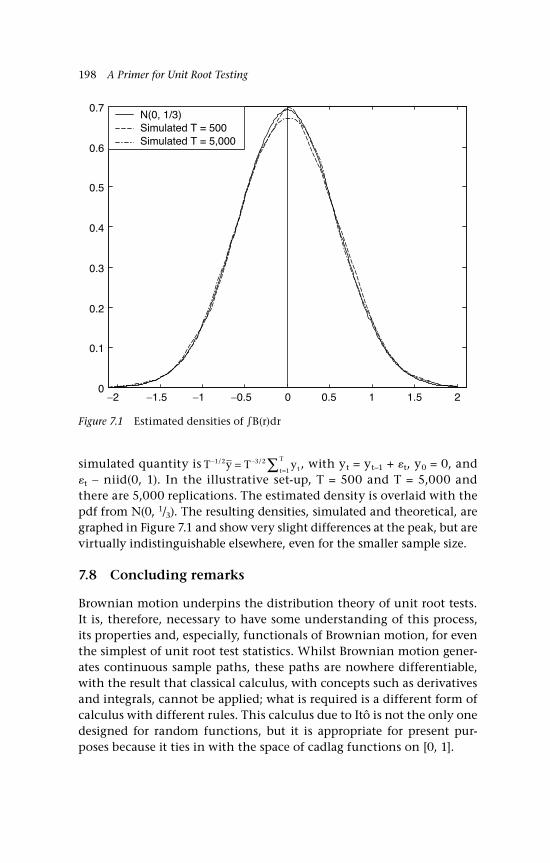
198 A Primer for Unit Root Testing
simulated quantity is T y T ytt
T− −=
= ∑1 2 3 2
1
/ / , with yt = yt–1 + t, y0 = 0, and t ∼ niid(0, 1). In the illustrative set-up, T = 500 and T = 5,000 and there are 5,000 replications. The estimated density is overlaid with the pdf from N(0, 1/3). The resulting densities, simulated and theoretical, are graphed in Figure 7.1 and show very slight differences at the peak, but are virtually indistinguishable elsewhere, even for the smaller sample size.
7.8 Concluding remarks
Brownian motion underpins the distribution theory of unit root tests. It is, therefore, necessary to have some understanding of this process, its properties and, especially, functionals of Brownian motion, for even the simplest of unit root test statistics. Whilst Brownian motion gener-ates continuous sample paths, these paths are nowhere differentiable, with the result that classical calculus, with concepts such as derivatives and integrals, cannot be applied; what is required is a different form of calculus with different rules. This calculus due to Itô is not the only one designed for random functions, but it is appropriate for present pur-poses because it ties in with the space of cadlag functions on [0, 1].
−2 −1.5 −1 −0.5 0 0.5 1 1.5 20
0.1
0.2
0.3
0.4
0.5
0.6
0.7N(0, 1/3)Simulated T = 500Simulated T = 5,000
Figure 7.1 Estimated densities of B(r)dr
Brownian Motion: Differentiation and Integration 199
In conventional integration, the ordinary Reimann integral of a func-tion f(t) can be viewed as the limiting value of a weighted sum, which is obtained as follows. First create a partition of the evaluation interval, for example t ∈ [0, 1], into n smaller intervals ti and then compute the weighted sum of the ti, where the weights are the function evaluations at points si, where si ∈ ti, say f(si). Taking si as the left-end point, ti–1, the right-end point, ti, the middle point or some other point in the interval, will not affect the limiting value of the weighted sum (where the limit refers to making the partition finer and finer). This is not the case if the function to be evaluated involves a Brownian motion input. The Itô calculus results from taking the left-end point for the evaluation of the weighted sum, which can be viewed as a non-anticipative choice; in terms of stochastic finance this relates to the opening position, and in terms of the distribution theory for partial sums it relates to the sum to the integer part of rT, where T is the sample size and r ∈ [0, 1]. The end result is that a correction, the Itô correction, is required to obtain the stochastic integral compared to the classical case where the function components are entirely non-random.
A particular interest in econometrics is the distribution of quan-tities such as sample moments and test statistics that arise in least squares and maximum likelihood estimation of AR and ARMA models, a simple example being the DF test statistic T( – 1), when the null generating model is yt = yt–1 + t, y0 = 0 and t ∼ niid(0, 2). This can be expressed as the ratio of two functionals of Brownian motion, specifically the ratio of W r dW r( ) ( )
0
1
∫ to W r dr( )2
0
1
∫ ; recall that a functional takes a function as its argument and maps this into a scalar, integrals being a classic example. The power driving various results in asymptotic distribution theory for unit root test statis-tics is then a combination of the central limit theorem (CLT) and the continuous mapping theorem (CMT), extended to functionals, see Chapter 6, Sections 6.6.1 and 6.6.2, respectively. Together these provide many of the results that have become standard in unit root testing.
There are number of books to which the reader may turn for an elaboration of the concepts introduced in this chapter. A selective and partial list follows. An excellent place to start for a review of classical calculus, and its extension to stochastic functions, is the introductory book by Mikosch (1998); this could usefully be followed by one of Brzezniak and Zastawniak (1999), Henderson and Plaschko (2006) and Kuo (2006); these books include important material on martingales and also include examples from economics, finance and
200 A Primer for Unit Root Testing
engineering. Continuing the finance theme, the reader could consult Shreve (2004) and Glasserman (2004). Books with a more explicit econometric orientation include Banerjee et al. (1993), McCabe and Tremayne (1993), Hamilton (1994) and Davidson (1994, 2000); the most extensive in terms of the probability background being Davidson (1994).
Questions
Q7.1 Generalise the Ornstein-Uhlenbeck process so that the implied long-run equilibrium can be non-zero.
A7.1 The basic Ornstein-Uhlenbeck process is, see Equation (7.30):
dX t X t dt dB t( ) ( ) ( )= +
with integral solution, see Equation (7.35), as follows:
X t e X e e dB st t st( ) ( ) ( )= + −∫ 0
0
In this specification, X(t) evolves as a function of its level and a sto-chastic input, which is scaled Brownian motion, with interpreted as a constant volatility parameter. The analogous discrete-time process is an AR(1) model without drift. The change that is necessary is to relate the nonstochastic part of the driving force to the deviation of X(t) from its steady state, – X(t); in the simple version, which is Equation (7.30), µ = 0, so that the implied steady state is zero. The revised specification is:
dX t X t dt dB t( ) ( ) ( )= − +
The first term is now the deviation of X(t) from µ and θ characterises the speed of adjustment. If X(t) = µ, then X(t) only changes if the sto-chastic input is non-zero and if that is zero then X(t) = µ, justifying the description of µ as the equilibrium or steady state of X(t). Note that if µ = 0, then θ = –.
All that changes in obtaining the solution is that a(t) = – X(t), rather than X(t). To obtain the integral solution take Y(t) = f[t, X(t)] = etX(t), with derivatives: ft = Y(t), fX = et and fXX = 0. Then make the

Brownian Motion: Differentiation and Integration 201
appropriate substitutions into (7.29), as follows:
Y T Y Y t e X t dt e dB s
Y T Y
tT ss( ) ( ) ( ) [ ( )] ( )
( ) ( )
= + + − +
= +
∫ ∫0
0
0 0
e dt e dB s
Y T Y e e dB s
Y T
tT ss
t T ss
0 0
0 00
∫ ∫∫
+
= + +
( )
( ) ( ) ] ( )
( ) == + − + ∫Y e e dB sT ss( ) ( ) ( )0 1
0
Finally, reverse the original substitution X(t) = e–tY(t), to obtain:
X T e Y e e e e dB s
e X e
t T T T ss
t
( ) ( ) ( ) ( )
( )
= + − +
= + −
− − −
− −
∫
0 1
0
0
T T ss
T T ss
e e dB s
X e e e dB s
+
= + − +
−
− −
∫∫
( )
[ ( ) ] ( )
0
00
Notice that the solution for the simpler case with µ = 0, as in (7.35), obtains by making the substitution θ = –α.
Q7.2 Confirm the following results from Table 7.1:
i. T y W r drtt
T
D−
−=∑ ∫⇒21
2
1
2
0
1( )
ii. T y W r dW rt t D−
−∑ ∫⇒11 0
1 ( ) ( )
A7.2 First define the partial sum process of εt and its scaled equivalent given, respectively, by:
S r
Z rS r
T
T tt
rT
TT
( )
( )( )
[ ]≡
≡
=∑ 1
Then from the FCLT:
Z r B r rT D( ) ( )⇒ ≤ ≤0 1
i. Turning to the question and considering T ytt
T−−=∑21
2
1, it is also con-
venient to define YT(r) and note the associated convergence result:
Y rS r
TW r B rT
TD( )
( )( ) ( )≡ ⇒ =
202 A Primer for Unit Root Testing
The quantity of direct interest is Y r T S rT T( ) ( )2 1 2= . The terms of which are given by:
Y r y T r T
Y r T y T T r T
Y
T
T
( ) / /
( ) ( ) / / / /
202
21 2
212
0 0 1
1 2
= = ≤ <
= + = ≤ <
TT jj
T
T
T jj
T
r T y T T T r
Y r
( ) / / ( )/
( ) /
2 2
1
1
12
2 2
1
1 1= ( ) = − ≤ <
= ( )=
−−
=
∑∑
TT y T rT= =2 1/
Note that r changes by 1/T each time a further step is taken. Taking the sum of these terms each weighted by 1/T is the first step in obtaining the integral:
y TT
T ytt
T
tt
T2
1
2 2
1
1/
=−
=∑ ∑( ) =
The integral of YT(r)2 with respect to r ∈ [0, 1], Y r drT( )2
0
1
∫ , is the limit of the last expression. Then from the FCLT applied to YT(r) and the CMT applied to YT(r)2 it follows that:
Y r dr W r dr B r drT D( ) ( ) ( )2
0
1 2
0
1 2 2
0
1
∫ ∫ ∫⇒ =
T ytt
T−=∑2 2
1 differs from T y T yt tt
T
t
T−−
−=
−
== ∑∑2
12 2 2
1
1
1 by one term, that is y2
T/T2, which is asymptotically negligible, so both T ytt
T−=∑2 2
1 and
T y W r dr B r drtt
T
D−
−=∑ ∫ ∫⇒ =21
2
1
2
0
1 2 2
0
1( ) ( ) .
ii. Turning to the second part of the question consider T yt−
−∑11.
Note that y2t = (yt–1 + t)2 = (y2
t–1 + 2yt–1t + 2t), therefore, yt–1t = 1–2(y
2t – y2
t–1 + 2
t). Hence, making the substitution:
T y
T y y
T y y
t t
t t tt
T
t tt
T
−−
−−=
−−=
∑∑
∑= − +
= − +
11
12
1 21
2 2
1
12
1 21
2
1
( )
ttt
T
t
T
T tt
TT y
2
11
12
1 2 2
1
==
−=
∑∑∑
( )= −( )
)
Brownian Motion: Differentiation and Integration 203
Noting from Table 7.1 that T–1y2T ⇒D W(1)2 = 2B(1)2 = 22 (1) as B(1) ~
N(0, 1); also p T tt
Tlim −
=∑( ) =1 2
1
2 , it then follows that:
T y Bt t D−
−∑ ⇒ −( ) −( )11
2 2 212
1 112
1 1 ( ) ~ ( )
Q7.3 Prove that if W(r) is Brownian motion, then V(r) = W(r) – rW(1) is a Brownian bridge.
A7.3 First note that V(r) has zero expectation:
E[V(r)] = E[W(r)] – rE[W(1)] = 0
The first term and second terms are zero by the property of Brownian motion:
cov[V(s), V(r)] = E[W(s) – sW(1)][W(r) – rW(1)]= E[W(s)W(r)] – rE[W(s)W(1)] – sE[W(r)W(1)] + rsE[W(1)2]= (s – rs – sr + rs)2
= s(1 – r)2
where s < r has been assumed. The result follows on noting that E[W(s), W(r)] = cov[W(s), W(r)] = s2 for s < r. Hence, the first and second moments are the same as for a Brownian bridge and as V(r) is Gaussian, V(r) is a Brownian bridge; see Ross (2003, chapter 10).
Q7.4 Prove the following:
S r
TB r rB V rT y
yD
, ( )( ) ( ) ( )
⇒ − ≡1 1
where S r y y y iidT y tt
rT
t y,
[ ]( ) ( ) ~ ( , ).= −
=∑ 1
2and
A7.4 Starting from the definition of ST,y~(r):
S r y y
y rT y T
y r
T y jt
rT
tt
rT
tt
T
tt
r
,
[ ]
[ ]
[
( ) ( )
[ ] /
= −
= −
= −
=
= =
=
∑∑ ∑
1
1 1
1
TT
tt
T
py o T]
( )∑ ∑ =+
1
204 A Primer for Unit Root Testing
Hence, noting that:
( ) ( )[ ]
y tt
rT
DT y B r−=∑ ⇒1
1 and ( ) ( ) ( ) ( ), T y T S Btt
T
T y D−
=−∑ = ⇒1
1
1 1 1
then the required result follows:
S r
TB r rB rT y
yD
, ( )( ) ( ) [ , ]
⇒ − ∈1 0 1
which is a standard first level Brownian bridge.
8Some Examples of Unit Root Tests
205
Introduction
It is not the intention in this chapter to provide a comprehensive review of unit root tests; that would be a task far more substantial than space allows. Rather, the idea is to introduce some tests that link in with developments in earlier chapters. Examples are given of two types of test: parametric and nonparametric. In the former case, probably the most frequently applied test is a version of the standard t test due to Dickey-Fuller (DF) tests, usually referred to as a test. This is a pseudo-t test in the sense that whilst it is constructed on the same general princi-ple as a t test, it does not have a t distribution under the null hypothesis of a unit root. A closely related test is the coefficient or normalised bias test, referred to here as a test, which is just T times the numerator of the pseudo-t statistic. Whilst the test is generally more powerful than the test, it is not so stable when the error process in the underlying model has a serially correlated structure, and is not so widely used as the test.
One of the problems of testing a hypothesis that a parameter takes a particular value under the null hypothesis is that power, the probabil-ity of rejecting the null hypothesis when the alternative hypothesis is correct, is likely to be low for alternatives very close to the null value. This is a problem generic to testing hypotheses that a parameter takes a particular value. In context, it means that processes with a near-unit root are going to be very difficult to discover. Tests for a unit root are very vulnerable to this criticism and the DF tests are known to have low power for near-unit root alternatives. Thus, one fruitful line of develop-ment has been to obtain tests that are more powerful. The second set of parametric tests described here, due to Elliott, Rothenberg and Stock
206 A Primer for Unit Root Testing
(1996) and Elliott (1999), gain power by demeaning or detrending the time series for an alternative close to the unit root.
There are also several nonparametric tests for a unit root. The one outlined here is due to Burridge and Guerre (1996), extended by García and Sansó (2006). The principle underlying this test is based on the intuition provided by Chapter 5 that random walks have infrequent mean reversion. We saw in Chapter 5, Section 5.6 that it was possi-ble to obtain the distribution of the number of sign changes for a ran-dom walk; hence, in principle, a test for a unit root can be based on the number of sign changes observed in a time series. Nonparametric tests are unlikely to be more powerful than parametric tests when the assumptions underlying the latter are correct, however they often have an appealing intuitive rationale and may have features that make them useful in combination with parametric tests.
This chapter is organised as follows. The basic testing framework is outlined in Section 8.1 and is extended in Section 8.2 to consider how to deal with deterministic terms that are particularly likely to be present under the alternative hypothesis. In a practical application of a unit root test, it is usually necessary to consider the possibility of dynamics in the error term and Section 8.3 considers this complication. An alternative family of unit root tests, based on ‘efficient’ detrending, is considered in Section 8.4. A nonparametric test, based on the observed number of crossings of a particular level, is considered in Section 8.5.
8.1 The testing framework
We consider the simplest case first to lay out a framework that is easily modified for more complex cases.
8.1.1 The DGP and the maintained regression
The simplest DGP of interest is that of the pure random walk:
y y ut t t= +−1 (8.1)ut t= (8.2)
The specification in (8.2) just sets ut to the special case of white noise, with finite variance, but allows for the more general case when ut ≠ t to be developed in later sections. Equation (8.1) is the special case of the following AR(1) model, with = 1:
y yt t t= +− 1 (8.3)
Some Examples of Unit Root Tests 207
Hence, = 1 corresponds to the unit root. We could proceed by estimat-ing (8.3) and setting up the null hypothesis H0 : = 1 to be tested against the alternative hypothesis HA : | | < 1. In this specification, the case = –1 is excluded from the parameter space under HA, since it also corresponds to a negative unit root, with unit modulus; however, notwithstanding this point, the alternative hypothesis is usually just specified as HA : < 1 on the understanding that the relevant part of the parameter space under HA is likely to be that which is close to the positive unit root.
The regression that is estimated in order to form a test statistic is referred to as the maintained regression; thus, in the present context, (8.3) is the maintained regression in order to test H0 : = 1 against HA : < 1. As it is generally easier to test a null hypothesis that a coefficient is equal to zero, yt–1 is subtracted from both sides of (8.3), to obtain:
y y
yt t t
t t
= − +
= +−
−
( )
1 1
1
(8.4)
where = ( – 1). The corresponding null and alternative hypotheses are now: H0 : = 0 against HA : < 0. HA is sometimes written more explicitly to indicate that the negative unit root is excluded, so that –2 < < 0.
Whilst a good place to start to establish some general principles, spec-ifying the maintained regression as in (8.3) is unlikely in practice. The reason for this is that the specification under HA summarises our view of how the data has been generated if the generating process is station-ary. Thus, for (8.3) to be relevant for < 1, there must be reversion to a mean of zero rather than to a non-zero mean; whilst there might (rarely) be good reasons to impose such a feature of the DGP under HA, if its imposition is invalid, so that the maintained regression should include an intercept, then the power of standard unit root tests, such as the pseudo-t, will tend to zero as the absolute value of the intercept increases. In intuitive terms, the presence of an intercept under HA, which is not included in the maintained regression, leads the test statis-tic to interpret the data as being generated by a nonstationary process.
8.1.2 DF unit root test statistics
The reason for starting with the simple case represented by Equations (8.1) – (8.3) is that they provide an introduction to obtaining the dis-tribution of two well-known unit root test statistics and the use of the FCLT and CMT. The two test statistics are the normalised bias and the
208 A Primer for Unit Root Testing
t-type test statistic, denoted and , respectively. These are:
ˆ ( ˆ ) = −T 1 (8.5)
ˆ( ˆ )
ˆ( ˆ)
= − 1
(8.6)
where is the LS estimator of and ˆ() is the estimated standard error of .
We will consider first. The LS estimator , – 1 and are, respec-tively, given by:
= −=
−=
∑∑
y y
y
t tt
T
tt
T
11
12
1 (8.7)
ˆ( )
− =−
=
− −=
−=
−=
−=
∑∑
∑∑
1 1 11
12
1
11
12
1
y y y
y
y
y
t t tt
T
tt
T
t tt
T
tt
T
usinng y yt t t− =−1
(8.8)
ˆ ( ˆ )
/
/
≡ −
=
=
−=
−=
−=
−=
∑∑
∑∑
T
Ty
y
y T
y
t tt
T
tt
T
t tt
T
tt
T
1
11
12
1
11
12
1
TT2
(8.9)
The numerator and denominator on the right-hand-side of this inequal-ity are familiar from Chapter 7.
There are several variants of a set of sufficient assumptions that lead to the same limiting null distributions of and , and the extensions of these statistics to include deterministic regressors. For example, from Fuller (1996, Theorem 10.1.1) we may specify that st1 is a martingale difference sequence, MDS, see Chapter 3, Section 3.5.1, as follows:
E
E
E K
t
t
t
( | )
( | )
(| | )
F
F
F
t
t
t
11
21
1 2
21
1
0−
−
+ −
=
= < ∞
= =
Some Examples of Unit Root Tests 209
where > 0, K is a finite constant and Ft1 is the –field generated by st1
(see Chapter 1, Section 1.2.3 for the definition of a –field). Alternatively, it may be assumed that t ~ iid(0, 2). Additionally y0 is assumed to be a finite constant, which is satisfied for cases such as y0 = 0, or y0 is a bounded random variable. The set of assumptions, which relate to the invariance of the functional central limit theorem, outlined in Chapter 6, Section 6.6.1, can also be adopted.
Considering (8.9), the limiting distributions of interest can be read off from Table 7.1 of Chapter 7:
T y W r dW r Bt tt
T
D−
−=∑ ∫⇒ = −111 0
11
22 21 1 ( ) ( ) ( )
(8.10)
T y W r dr B r drtt
T
D−
−=∑ ∫ ∫⇒ =21
2
1
2
0
1 2 2
0
1( ) ( )
(8.11)
These are the limiting distributions of the numerator and denominator quantities of and the next question is whether the limiting distribu-tion of the ratio is the ratio of the limiting distributions. This follows from the CMT extended to function spaces, see Chapter 6, Section 6.2.2 and, for example, Davidson (2000, Theorem 14.2.3) and Billingsley (1995, Theorem 25.7), so that:
ˆ( ) ( )
( )( ˆ)
( )
( )
⇒ ≡
= −
∫∫
∫
D
B r dB r
B r drF
B
B r dr
0
1
2
0
1
12
2
2
0
1
1 1
(8.12)
Notice that the second line uses the result that B r dB r B( ) ( ) [ ( ) ]0
112
21 1∫ = − , see Chapter 7, Equation (7.11).
Whilst the limiting distribution of the numerator of (8.12) exists in closed form, see Chapter 7, Table 7.1, this is not the case for the denomi-nator so that, in practice, the percentiles are obtained by simulating the distribution function, as in Fuller (1976, 1996). This is considered in more detail in the next section and in an appendix.
Perhaps the most frequently used test statistic for the unit root null hypothesis is , the t-statistic based on , sometimes referred to as a pseudo-t statistic in view of the fact that its distribution is not the ‘t’ distribution. The numerator of is and the denominator is (), the
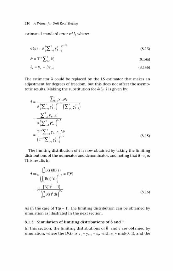
210 A Primer for Unit Root Testing
estimated standard error of , where:
ˆ( ˆ)/
= ( )−=
−
∑ ytt
T
12
1
1 2
(8.13)
= −=∑T tt
T1 2
1
(8.14a)
ˆ ˆt t ty y= − − 1 (8.14b)
The estimator ~ could be replaced by the LS estimator that makes an adjustment for degrees of freedom, but this does not affect the asymp-totic results. Making the substitution for (), is given by:
ˆ /
=( ) ( )
=
−=
−=
−
−=
−=
∑∑ ∑∑
y
y y
y
t tt
T
tt
T
tt
T
t tt
T
11
12
1
1 2
12
1
11
yy
T y
T y
tt
T
t tt
T
tt
T
−=
−−=
−−=
∑∑∑
( )=
( )
12
1
1 2
111
21
2
1
1 2
/
/
/
(8.15)
The limiting distribution of is now obtained by taking the limiting distributions of the numerator and denominator, and noting that ~ →p . This results in:
ˆ( ) ( )
( )(ˆ)
[ ( ) ]
( )
/ ⇒
( )≡
= −
∫∫
D
B r dB r
B r drF
B
B r dr
0
1
2
0
1 1 2
12
2
2
0
1
1 1
∫∫( )1 2/
(8.16)
As in the case of T( – 1), the limiting distribution can be obtained by simulation as illustrated in the next section.
8.1.3 Simulation of limiting distributions of and
In this section, the limiting distributions of and are obtained by simulation, where the DGP is yt = yt–1 + t, with t ~ niid(0, 1), and the

Some Examples of Unit Root Tests 211
maintained regression is yt = yt–1 + t; note that the test statistics are invariant to 2 so that, for convenience, it may be set equal to unity. The test statistics are obtained for and for T = 1,000 and 5,000 rep-lications. Figure 8.1 shows the simulated cdf of , from which a skew to the left, inherited from the distribution of ( – 1), is evident. The corresponding pdf is shown in Figure 8.2; although the mode is zero, the distribution is not symmetric. The estimated 1%, 5% and 10% percentiles for are: –13.2(–13.7), –8.1(–8.1), –5.8(–5.7), respectively; these are very close to the percentiles from Fuller (1996, table 10A.1), shown in parentheses and obtained from a larger number of replica-tions. Figure 8.3 shows the simulated cdf of , together with the cdf of the standard normal distribution; and Figure 8.4 shows the corre-sponding pdfs. The distribution of is shifted to the left compared to the normal distribution, with the result that the critical values typi-cally used for testing are more negative than those from the standard normal distribution. The estimated 1%, 5% and 10% percentiles for are: –2.58, –1.95 and –1.62, which are identical to the percentiles from Fuller (1996, table 10A.1).
−20 −15 −10 −5 0 50
0.1
0.2
0.3
0.4
0.5
0.6
0.7
0.8
0.9
1
obtaining the 10% critical value = −5.8
Figure 8.1 Simulated distribution function of
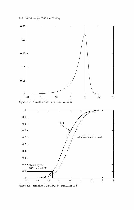
212 A Primer for Unit Root Testing
−20 −15 −10 −5 0 5 100
0.05
0.1
0.15
0.2
0.25
−4 −3 −2 −1 0 1 2 3 40
0.1
0.2
0.3
0.4
0.5
0.6
0.7
0.8
0.9
1
cdf of standard normal
cdf of τ
obtaining the10% cv = −1.62
Figure 8.2 Simulated density function of
Figure 8.3 Simulated distribution function of

Some Examples of Unit Root Tests 213
8.2 The presence of deterministic components under HA
It is rarely the case that under the alternative hypothesis, the time series of interest reverts to a zero mean in the long run. Two more likely cases are that of long-run reversion to a constant and, alternatively, reversion to a trend. Economic examples in the former case include unemploy-ment and real inflation rates, and in the latter case many macroeco-nomic series formed by aggregating individual components, such as consumption expenditure and GDP.
8.2.1 Reversion to a constant or linear trend under the alternative hypothesis
As noted in Section 8.1.1, the case where the maintained regression does not contain any deterministic terms is likely to be the exception rather than the rule. The two most familiar cases are t = and t = 0 + 1t, corresponding to AR(1) models of the following form:
y yt t t− = − +− ( )1 (8.17)
y yt t t t t− = − +− − ( )1 1 (8.18a)
Figure 8.4 Simulated density function of
−4 −3 −2 −1 0 1 2 3 40
0.05
0.1
0.15
0.2
0.25
0.3
0.35
0.4
0.45
pdf of standard normal pdf of τ

214 A Primer for Unit Root Testing
t t= +0 1 (8.18b)
First, consider the specification in (8.17): then according to H0, = 1, which reduces (8.17) to (8.3), the data is generated by a pure random walk; however, according to HA, the data has the characteristics of a stationary process, but with a non-zero, long-run mean, , to which the stationary series reverts. Second, in the case of (8.18) under HA, the stationary series reverts to a linear trend.
Figures 8.5 and 8.6 show two simulated series for T = 500, each gener-ated by a stationary but near-unit root process with = 0.975, that revert to a constant mean or to a trend, respectively. In the first case, the DGP is as in (8.17) with = 10 and in the second as in (8.18) with 0 = 10 and 1 = 0.1, where t ∼ niid(0, 1) in both cases. Note from Figure 8.5, that the near-unit root leads to long sojourns away from the long-run mean and from Figure 8.6 that whilst the trend is the attractor, there are long periods when observations are away from the trend.
What is evident from these figures is that the maintained regres-sion must include a mechanism that is capable of capturing the behaviour of yt according to HA as well as according to H0. As a result,
0 50 100 150 200 250 300 350 400 450 500−5
0
5
10
15
20
Time
yt
µ
Figure 8.5 Data generated by a stationary mean-reverting process
Note: Near-unit root leads to long periods away from the long-run mean, = 10
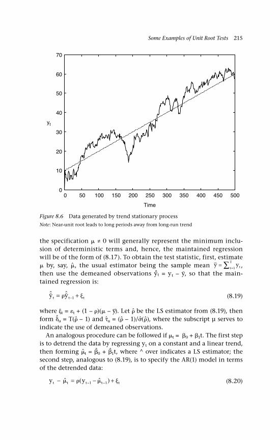
Some Examples of Unit Root Tests 215
the specification ≠ 0 will generally represent the minimum inclu-sion of deterministic terms and, hence, the maintained regression will be of the form of (8.17). To obtain the test statistic, first, estimate by, say, , the usual estimator being the sample mean y ytt
T=
=∑ 1 , then use the demeaned observations y~t = yt – y–, so that the main-tained regression is:
ˆ ˆy yt t t= +− 1 (8.19)
where t = t + (1 – )( – y–). Let be the LS estimator from (8.19), then form u = T( – 1) and u = ( – 1)/(), where the subscript µ serves to indicate the use of demeaned observations.
An analogous procedure can be followed if t = 0 + 1t. The first step is to detrend the data by regressing yt on a constant and a linear trend, then forming t = 0 + 1t, where ^ over indicates a LS estimator; the second step, analogous to (8.19), is to specify the AR(1) model in terms of the detrended data:
y yt t t t t− = − +− −ˆ ( ˆ ) 1 1 (8.20)
0 50 100 150 200 250 300 350 400 450 5000
10
20
30
40
50
60
70
Time
yt
Figure 8.6 Data generated by trend stationary process
Note: Near-unit root leads to long periods away from long-run trend
216 A Primer for Unit Root Testing
The test statistics are formed as in the case of (8.19), but are distin-guished by the subscript as and , to indicate that a linear trend has been removed from the observations.
The limiting distributions of the test statistics, which assume that the DGP according to the null is yt = t, are as follows:
ˆ( ) ( )
( )( ˆ ) i D
i i
i
i
B r dB r
B r drF⇒ ≡∫
∫0
1
2
0
1
(8.21)
ˆ( ) ( )
( )(ˆ )/ i D
i i
i
i
B r dB r
B r drF⇒
( )≡∫
∫0
1
2
0
1 1 2
(8.23)
where i = µ, and the functionals of Brownian motion are as follows:
B r B r B s ds
B r B r r B s ds r sB s
( ) ( ) ( )
( ) ( ) ( ) ( ) ( ) (
= −
= + − − −
∫∫
0
1
0
16 4 12 6 ))ds
0
1
∫
Notice that B(r) and B(r) are demeaned and detrended Brownian motion, as defined in Chapter 7, Equations (7.45) and (7.49), respectively; thus, the limiting distributions are of the same form as in (8.12) and (8.16) except for the substitution of the appropriate form of Brownian motion. The critical values of these distributions have been obtained by simulation see, for example, Fuller (1996, Appendix A); a response func-tion approach to obtaining the critical values (quantiles) is described in the appendix to this chapter.
The simulated pdfs of , and are shown in Figure 8.7 for T = 100. Note the leftward shift in the density functions as the number of deter-ministic terms is increased. For example, the 5% quantiles are: –1.95, –2.90 and –3.45 for , and , respectively. Simulated power for T = 100 for the DF tests is shown in Figure 8.8. (The initial observation is drawn from the unconditional distribution of ut; for more discussion of this point, see Section 8.4.) Notice that power declines substantially as more deterministic terms are included, with power() ≤ power() ≤ power(); for example, estimated power at = 0.9 is 83% for , 35% for and 20% for . Much of the research on different unit root test statistics has been directed to obtaining test statistics that improve on the power of the DF tests, and we outline one such approach in Section 8.4.
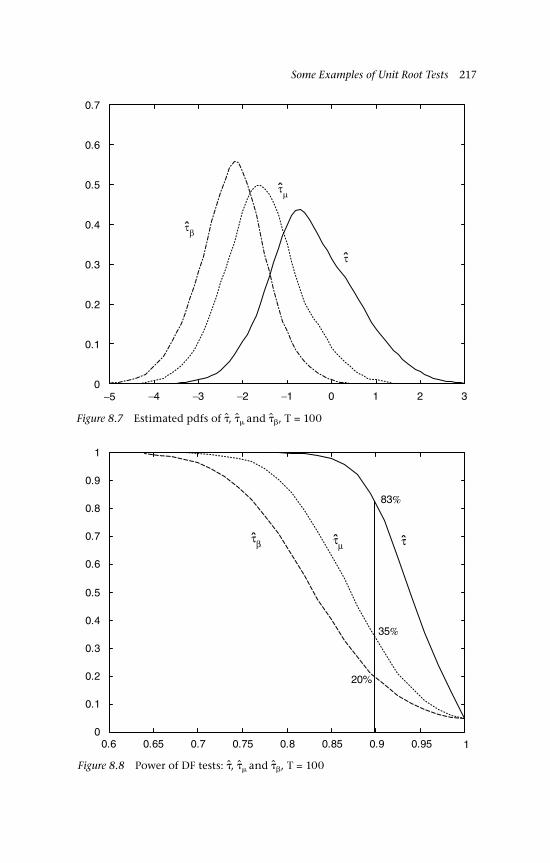
Some Examples of Unit Root Tests 217
−5 −4 −3 −2 −1 0 1 2 30
0.1
0.2
0.3
0.4
0.5
0.6
0.7
τµ
τβˆ
ˆ
τ
Figure 8.7 Estimated pdfs of , and , T = 100
0.6 0.65 0.7 0.75 0.8 0.85 0.9 0.95 10
0.1
0.2
0.3
0.4
0.5
0.6
0.7
0.8
0.9
1
µβ
83%
35%
20%
τ τ τ
Figure 8.8 Power of DF tests: , and , T = 100

218 A Primer for Unit Root Testing
8.2.2 Drift and invariance: The choice of test statistic and maintained regression
There are two typical cases in which unit root tests are used. In the first, the issue is to decide whether an observed time series is best described as being generated by a process with a unit root, but no drift, or a sta-tionary process that generates observations that would, in equilibrium, revert to a constant, non-zero mean, see, for example, the pattern graphed in Figure 8.5 for a stylised view of the data. In this case, a test statistic based on Equations (8.19) or (8.20) would be appropriate, perhaps subject to an extension for possible serial correlation, which is described in Section 8.3 below.
In the second case, the observed data has a trend, which must be capable of explanation in terms of a nonstationary process and, alter-natively, in terms of a stationary process. As to the former, there are two possibilities, the first is that the underlying random walk does not inherently have a direction, but the direction it has taken is just as likely as any other and so provides an ex post explanation of the observed data. This explanation is not entirely satisfactory, as it suggests that if another ‘run’ of history was possible we might observe a trend in the opposite direction. Evidently, this would be a difficulty for series such as GDP and consumption!
Alternatively, the direction has been driven by drift in the random walk process, for example positive drift for GDP. According to the expla-nation under HA, the direction is accounted for by a linear trend (or other polynomial trend) and once the data is adjusted for this trend, a stationary series results. Thus, the competing explanations are matched in terms accounting for a central feature of the observed data. The practical implication of the explanation under H0 is that an appropri-ate DGP would be yt = + t, rather than yt = t, and a desirable characteristic of any unit test statistic in this context is that its limiting null distribution should be invariant to , otherwise, with unknown, there would be a problem in determining the appropriate critical val-ues. To achieve this invariance, the maintained regression including a linear trend must be used, which would reduce to yt = + t, = 0, according to the null hypothesis. The resulting DF test statistics are and . The test statistics and are not invariant to , whereas the limiting null distributions of and are invariant to ; as a corollary, this invariance means that may be set equal to zero in obtaining the percentiles required for hypothesis testing. This method is part of a general procedure in that including in the maintained regression a
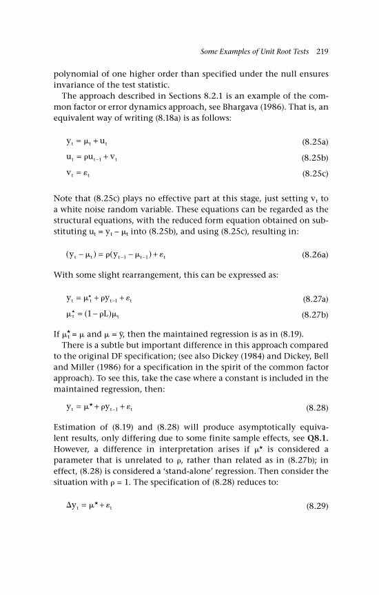
Some Examples of Unit Root Tests 219
polynomial of one higher order than specified under the null ensures invariance of the test statistic.
The approach described in Sections 8.2.1 is an example of the com-mon factor or error dynamics approach, see Bhargava (1986). That is, an equivalent way of writing (8.18a) is as follows:
y ut t t= + (8.25a)
u u vt t t= +− 1 (8.25b)
vt t= (8.25c)
Note that (8.25c) plays no effective part at this stage, just setting vt to a white noise random variable. These equations can be regarded as the structural equations, with the reduced form equation obtained on sub-stituting ut = yt – t into (8.25b), and using (8.25c), resulting in:
( ) ( )y yt t t t t− = − +− − 1 1 (8.26a)
With some slight rearrangement, this can be expressed as:
y yt t t t= + +− * 1 (8.27a)
t tL* ( )= −1 (8.27b)
If *t = and = y–, then the maintained regression is as in (8.19).There is a subtle but important difference in this approach compared
to the original DF specification; (see also Dickey (1984) and Dickey, Bell and Miller (1986) for a specification in the spirit of the common factor approach). To see this, take the case where a constant is included in the maintained regression, then:
y yt t t= + +− * 1 (8.28)
Estimation of (8.19) and (8.28) will produce asymptotically equiva-lent results, only differing due to some finite sample effects, see Q8.1. However, a difference in interpretation arises if * is considered a parameter that is unrelated to , rather than related as in (8.27b); in effect, (8.28) is considered a ‘stand-alone’ regression. Then consider the situation with = 1. The specification of (8.28) reduces to:
yt t= +* (8.29)
220 A Primer for Unit Root Testing
whilst that of (8.19) reduces to:
yt t= (8.30)
Note that (8.29) includes a drift term *, implying a deterministic trend in yt as well as the stochastic trend from the cumulated values of current and lagged t, whereas (8.30) just implies the latter. If (8.29) is what is regarded as the most likely specification under the null, perhaps informed by a prior graphical analysis, then the maintained regression should include a linear trend, as follows:
y y tt t t= + + +− * *1 (8.31)
The specification in (8.29) can then be tested by an F-type test that jointly tests = 1 and * = 0. Dickey and Fuller (1981) suggested such a test and a number of other joint tests, and provided some critical values; see also Patterson (2000) for critical values.
Also, unless * = (1 – ) is imposed there will be a difference under HA in the two formulations. Consider the difference in a simulation set-up in order to assess power. In the common factor approach, the long-run mean, , is kept constant, whereas in the DF specification, the long-run mean varies because * is kept constant. Further, in order to ensure sta-tionarity under the alternative, the initial value, y0, should be a draw from N(, 2
y), where 2y = (1 – 2)–12 is the unconditional variance.
Schmidt and Phillips (1992) show that the power curves, for a given value of < 1 under HA, from the two approaches cross. For consistency of treatment of the deterministic components under H0 and HA, the common factor approach is preferred. For a more detailed discussion of the issues, especially power comparisons see Marsh (2007).
8.3 Serial correlation
The specification of the maintained regression has so far assumed that t is not serially correlated, implying 2
lr,v = 2. In practice, this may not be the case and so the testing procedure must be flexible enough to allow 2
lr,v ≠ 2. The approach we take here is to model vt as generated by the ARMA process, although it applies to more general linear processes, see Chang and Park (2002). The reduced form equation of the underly-ing system of structural equations that becomes the basis of the testing model is known as an augmented Dickey-Fuller, ADF, regression.

Some Examples of Unit Root Tests 221
In the case of serial correlation in vt, it transpires that the ratio /lr,v is a nuisance parameter that affects the null distribution of the -type statistic, both finite sample and limiting, but not that of the -type sta-tistic. In the former case, the limiting distribution of the DF -type test is a simple scalar multiple of the corresponding DF distribution and multiplying by (/lr,v)–1 = lr,v/ gives a test statistic with a DF distri-bution; thus, to obtain a feasible test statistic, a consistent estimator of /lr,v is required.
8.3.1 The ADF representation
A leading specification for vt is that it is generated by a stationary and invertible ARMA process. The structural equations are now:
y ut t t= + (8.32a)
u u vt t t= +− 1 (8.32b)
& ( ) ( )L v Lt t= (8.32c)
where & &( )L Lii
p i= −=
−∑11
1, ( )L Ljj
q j= +=∑1
1 and &(L) and (L) are assumed to be invertible. From (8.32c) we can obtain that 2
lr,v = [(1)/&(1)]22; (see Chapter 2, Section 2.6.2 and note that here we are obtaining the long-run variance of vt).
To obtain the reduced form of (8.32a)−(8.32c), first, as usual, define y~t ≡ yt – t and then substitute yt from (8.32a) into (8.32b) and use (8.32c), to obtain:
& ( )( ) ( )L L y Lt t1 − = (8.33)
⇒
=( )L yt t (8.34)
where (L) = (L)–1&(L)(1 – L). The order of (L) will be infinite if (L)is of order q ≥ 1 or if &(L) is of infinite order. The AR form of (8.34), and the general nature of (L), should be familiar from Chapter 2.
It is convenient to write (L) as (L) = 1 – (L), where ( )L Lii
j==
∞∑ 1.
Next, a useful representation of (L) is through the DF decomposition:
( ) ( ) ( )( )L L c L L= + −1 1 (8.35)

222 A Primer for Unit Root Testing
where c L c Ljj
j( ) ==
∞∑ 1. Using this decomposition, the original form, (8.34),
can be separated into two parts, once comprising the lag of y~t and the other comprising lags of y~t. Then, substituting (8.35) in (8.34), we obtain:
y y c L yt t t t= + +−( ) ( )1 1 (8.36)
⇒= + +− y y c L yt t t t 1 ( ) (8.37)
where = (1) – 1. Note that if there is a unit root, then (1) = 1 (see Chapter 2, Section 2.1.3), implying that = 0, which forms the basis of using the pseudo-t test on as a unit root test, where is the LS estima-tor from a feasible version of (8.37).
The form of the model in (8.37) is known as an augmented Dickey-Fuller (ADF) regression. If the original AR order in (8.34) is AR(p), p < ∞, then the corresponding ADF model, (8.37), is ADF(p – 1), where (p – 1) is the order of the c(L) polynomial.
To proceed to a feasible model, first assume that c(L) is of infinite order, so that (8.37) is:
y y c yt t jj t j t= + +− =
∞−∑ 1 1
(8.38)
This cannot be estimated because of the infinite number of lags on yt, so a truncation rule is required to ensure a finite order for c(L), resulting in, say, an ADF(p – 1) model, as follows:
y y c yt t jj
p
t j t p= + +− =
−−∑ 1 1
1 ,
(8.39)
t p jj p t j tc y, = +=
∞−∑
(8.40)
A condition is required on the expansion rate for p* = p – 1, so that p* increases with the sample size. A sufficient condition in this case has already been considered in Chapter 2, Section 2.6.2 (see below Equation (2.51)); it requires that p*/T1/3 → 0 as T → ∞, and there exist constants, and s, such that p* > T1/s, see Said and Dickey (1984), Xiao and Phillips (1998, Assumption A4). This expansion rate governs the case where T is variable, so it does not directly provide guidance in a single sample, where T is fixed. As noted in Chapter 2, a rule of the form

Some Examples of Unit Root Tests 223
p* = [K(T/100)1/3] is often used, with K = 4, 12, but the sensitivity of the results to increasing p* should be assessed.
8.3.2 Limiting null distributions of the test statistics
Let denote the LS estimator from (8.39) and let the pseudo-t be adf = /(), where () is the estimated standard error of , and assume that p* expands at the required rate. Then, it is still the case that the limiting null distribution of adf is the DF distribution, see Fuller (1996, Theorem 10.1.4), that is:
ˆ (ˆ) adfD F⇒ (8.41)
ˆ (ˆ ) adf
D F⇒ (8.42)
ˆ (ˆ ) adf
D F⇒ (8.43)
These results mean that the limiting percentiles are still those of the corresponding DF distribution; there are, however, differences in the finite sample distributions, which are sensitive to the lag length in the ADF regression, see Cheung and Lai (1995a, b) and Patterson and Heravi (2003), who provide critical values from a response surface approach.
It is not, however, the case that ~ = T has a DF limiting null distribu-tion. To achieve this result it is necessary to make an adjustment. Xiao and Phillips (1998, Theorem 1) show that the limiting null distribution of ~ is a scalar multiple of the DF distribution, that is:
ˆ( ) ( )
( )
( ˆ)
,
,
⇒
=
∫∫
Dlr v
lr v
B r dB r
B r dr
F
0
1
2
0
1
(8.44)
Notice that the ‘sigma’ ratio /lr,v is a nuisance parameter that scales the DF distribution, F(); thus, multiplying by the inverse of the sigma ratio removes the nuisance parameter from the asymptotic distribution. That is:
ˆ( ) ( )
( )
( ˆ)
,
adf lr vD
B r dB r
B r dr
F
≡ ⇒
=
∫∫0
1
2
0
1
(8.45)
224 A Primer for Unit Root Testing
As in the case of the pseudo-t tests, this result extends to the case where the data are demeaned or detrended, so that:
ˆ ( ˆ ),
adf lr vD F≡ ⇒
(8.46)
ˆ ( ˆ ),
adf lr vD F≡ ⇒
(8.47)
where ~
and ~
are as ~, but in the demeaned and detrended cases,
respectively.A feasible test statistic results from replacing lr,v and by consistent
estimators, denoted lr,v and , respectively. Estimation of the long run variance was considered in Chapter 2, Section 2.6. The parametric esti-mator of lr,v is a natural one to consider in this context. In the case of the ADF(p*) model of (8.39), 2
lr,v is obtained as follows:
ˆ( ˆ( ))
ˆ, lr v pc2
2
211 1
=−
(8.48)
ˆ ˆ ,p t pt p
TT2 1 2= −
=∑
(8.49)
where ˆ( ) ˆ , ˆ*c c cjj
p
j11
==∑ is the LS estimator of cj and t,p is the t-th residual
from estimation of (8.39). Hence, a consistent estimator of the inverse sigma ratio is given by:
ˆ
ˆ ˆ ( ˆ( ))ˆ
( ˆ( ))
,
lr v
ppc
c
=−
=−
1 11 1
11 1
(8.50)
This provides the required scalar multiple for (8.45), (8.46) or (8.47), so that:
ˆ ˆ
ˆ
ˆ( ˆ( ))
,
adf lr v
Tc
≡
−=
1 1 (8.51)
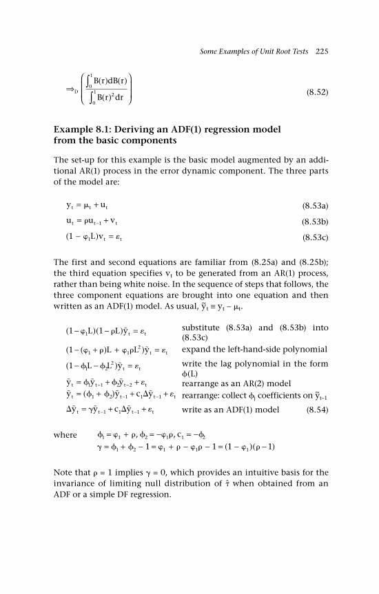
Some Examples of Unit Root Tests 225
⇒
∫∫
D
B r dB r
B r dr
( ) ( )
( )0
1
2
0
1
(8.52)
Example 8.1: Deriving an ADF(1) regression model from the basic components
The set-up for this example is the basic model augmented by an addi-tional AR(1) process in the error dynamic component. The three parts of the model are:
y ut t t= + (8.53a)
u u vt t t= +− 1 (8.53b)
( )1 1− =& L vt t (8.53c)
The first and second equations are familiar from (8.25a) and (8.25b); the third equation specifies vt to be generated from an AR(1) process, rather than being white noise. In the sequence of steps that follows, the three component equations are brought into one equation and then written as an ADF(1) model. As usual, y~t ≡ yt – t.
( )( )1 11− − =& L L yt t substitute (8.53a) and (8.53b) into (8.53c)
( ( ) )1 1 12− + + =& & L L yt t expand the left-hand-side polynomial
( )1 1 22− − = L L yt t
write the lag polynomial in the form (L)
y y yt t t t= + +− − 1 1 2 2 rearrange as an AR(2) modely y c yt t t t= + + +− −( ) 1 2 1 1 1
rearrange: collect j coefficients on y~t–1
y y c yt t t t= + +− − 1 1 1 write as an ADF(1) model
where & &
& & &
1 1 2 1 1 2
1 2 1 1 11 1 1 1
= + = − = −= + − = + − − = − −
, ,
( )( )
c
Note that = 1 implies = 0, which provides an intuitive basis for the invariance of limiting null distribution of when obtained from an ADF or a simple DF regression.
(8.54)

226 A Primer for Unit Root Testing
From = (1 – &1)( – 1), it is evident that:
( )( )
&− =
−1
1 1
Hence, if &1 is known, ( – 1) and, therefore, can be obtained. Under the null hypothesis c1 = &1 = &1, so that:
( )( )
− =−
11 1c
conditional on = 1
For example, suppose that t = 0 + 1t, then from estimation of (8.54), the type test statistic can be obtained as:
ˆ ˆ( ˆ )
adf
c=
−1 1
where adf has the limiting null distribution given in (8.47). Note that
this procedure fails under the alternative hypothesis; an alternative in that case is to estimate &1 and from (8.54) imposing the nonlinear constraints. ♦
Example 8.2: Deriving an ADF(∞) regression model from the basic components
In this example vt is modelled as generated from an invertible MA(1) process. This results in an ADF of infinite order and illustrates some principles that are applicable to higher order MA and infinite AR proc-esses. As before, there are three component equations:
y ut t t= + (8.55a)
u u vt t t= +− 1 (8.55b)
v Lt t= +( )1 1 (8.55c)
The reduced form can be obtained as follows:
( ) ( )1 1 1− = + L y Lt t substitute (8.55a) into (8.55b) and use (8.55c)
( ) ( )1 111+ − =− L L yt t the MA lag polynomial is invertible
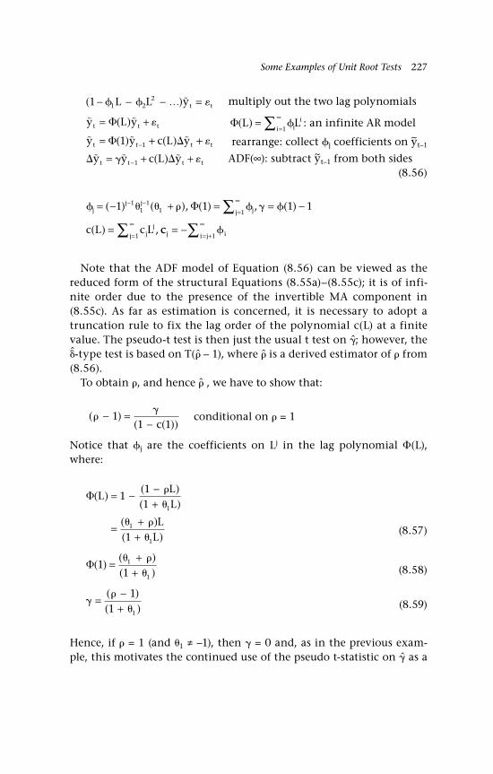
Some Examples of Unit Root Tests 227
( )1 1 22− − − = L L yt t multiply out the two lag polynomials
y L yt t t= +( ) ( )L Lii
i=
=
∞∑ 1: an infinite AR model
y y c L yt t t t= + +−( ) ( )1 1 rearrange: collect j coefficients on y~t–1
y y c L yt t t t= + +− 1 ( ) ADF(∞): subtract y~t–1 from both sides (8.56)
jj j
jj
jj
jc L c L
= − + = = −
=
− −=
∞
=
∞
∑∑
( ) ( ), ( ) , ( )
( ) ,
1 1 1 111
11 1
1ccj ii j
= −= +
∞∑ 1
Note that the ADF model of Equation (8.56) can be viewed as the reduced form of the structural Equations (8.55a)–(8.55c); it is of infi-nite order due to the presence of the invertible MA component in (8.55c). As far as estimation is concerned, it is necessary to adopt a truncation rule to fix the lag order of the polynomial c(L) at a finite value. The pseudo-t test is then just the usual t test on ; however, the -type test is based on T( – 1), where is a derived estimator of from (8.56).
To obtain , and hence , we have to show that:
( )( ( ))
− =−
11 1c
conditional on = 1
Notice that j are the coefficients on Lj in the lag polynomial (L), where:
( )( )( )
( )( )
LLL
LL
= −−+
=+
+
111
1
1
1
1 (8.57)
( )
( )( )
11
1
1
=+
+ (8.58)
=
−+
( )( )
11 1
(8.59)
Hence, if = 1 (and 1 ≠ –1), then = 0 and, as in the previous exam-ple, this motivates the continued use of the pseudo t-statistic on as a
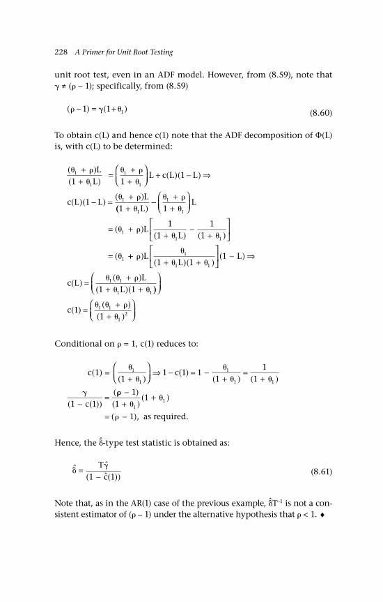
228 A Primer for Unit Root Testing
unit root test, even in an ADF model. However, from (8.59), note that ≠ ( – 1); specifically, from (8.59)
( ) ( ) − = +1 1 1 (8.60)
To obtain c(L) and hence c(1) note that the ADF decomposition of (L) is, with c(L) to be determined:
( )( )
( )( )
( )( )( )
1
1
1
1
1
1 11
1
++
=+
+
+ − ⇒
− =+
LL
L c L L
c L LL
(( )
( )( ) ( )
(
1 1
11
11
1
1
1
11 1
1
+−
++
= ++
−+
=
LL
LL
+++ +
− ⇒
=+
+ +
)( )( )
( )
( )( )
( )(
LL
L
c LL
L
1
1 1
1 1
1 1
1 11
1 1 ))
( )( )
( )
=+
+
c 111 1
12
Conditional on = 1, c(1) reduces to:
c(1) =
1
1
1
1 111 1 1
11
1
1 1
( )( )
( ) ( )
( ( ))(
+
⇒ − = −+
=+
−=
c
c
−+
+
= −
11
1
11
1
)( )
( )
( ), as required.
Hence, the -type test statistic is obtained as:
ˆ ˆ( ˆ( ))
=−T
c1 1 (8.61)
Note that, as in the AR(1) case of the previous example, T–1 is not a con-sistent estimator of ( – 1) under the alternative hypothesis that < 1. ♦
Some Examples of Unit Root Tests 229
8.3.3 Limiting distributions: Extensions and comments
The distribution results summarised in the previous section extend to linear processes, other than ARMA processes, of the form vt = (L)t where ( )L Ljj
j==
∞∑ 0, with (z) ≠ 0 for all |z| < 1 and | |j k
jj
=
∞∑ 0 < ∞ for some k ≥ 1, see Chang and Park (2002). The latter authors emphasise that conditional heterogeneous error processes, such as covariance sta-tionary ARCH and GARCH models, are permitted, and some forms of unconditional heterogeneity (see also Chapter 6, Section 6.6.3) as in the case of the modified test statistics suggested by Phillips and Perron (1988). Notably, in the present context, Chang and Park (op. cit.) derive that in the case of adf (but not
adf) the rate of expansion of the lag length in the ADF regression may be p* = o(T)1/2, compared to the Said and Dickey rate of p* = o(T)1/3. However, p* = o(T)1/2 is not sufficient for consistency of the LS estimators cj
p*j=1, so that lag selection techniques
that rely on this consistency require a slower rate of expansion. The required rate differs depending on the heterogeneity in the MDS, with p* = o(T/ln(T)1/2) for a homogenous MDS and p* = o(T)1/3 for a possibly heterogeneous MDS.
8.4 Efficient detrending in constructing unit root test statistics
A well-known problem with DF tests is that they lack power when the dominant root is close to unity. A uniformly powerful test across the whole range of values for does not exist, but power can be improved for a particular value of . This section describes one of a family of tests due to Elliott, Rothenberg and Stock (1996), hereafter ERS, and Elliott (1999). The idea is that when there is no UMP test, one possibility is maximise power for a given alternative very local to = 1 (see also Cox and Hinkley (1974)).
The method consists of two steps. In the first step, referred to as efficient detrending, the data is detrended by a GLS-type procedure for a fixed value c of , chosen such that c is ‘local-to-unity’ in a well-defined sense; in the second step, a unit root test is then carried out on the detrended data. There are a number of tests based on this idea and the one described here is the extension of the DF family of tests.
The idea of a near-integrated process, and the testing framework associated with it, is one in which under HA, takes a value that is ‘local-to-unity’. To capture this idea, consider the alternative hypothesis
230 A Primer for Unit Root Testing
specified as
H c TA c: / = = + <1 1 (8.62)
where c < 0 and c ∈ C, so that C is the set of possible values of c. For example, with T = 100, values of c = –5 and –10 imply c = 0.95 and c = 0.9, and as T increases c gets closer to unity. It is this part of the param-eter space where the power of standard unit root tests, such as and , have low power, see Figure 8.8.
In the local-to-unity framework, in principle, power can be maxim-ised for each value of c, which gives the power envelope, (c), that is the outer bound of power for c ∈ C. This seems to imply an infeasible pro-cedure since c is a continuous variable and there is, therefore, an infin-ity of tests indexed by c ∈ C. Consider one of these, so that c is fixed at, say, c* and a test statistic is constructed conditional on this value, then its power function, (c, c*) will be tangential to the power envelope at c = c*, but elsewhere will, generally, lie below it. It is then possible to choose a value for power, say 0.5, and solve (by simulation) for the value of c, say c–, that generates that value. ERS (op. cit.) suggest choosing c = c– correspond-ing to 50% power on the power envelope, so that (c, c–) = 0.5 and, there-fore, the test designed for c = c– will have a tangent to the power envelope at power = 50%. The form of such a test is outlined in the next two sections.
8.4.1 Efficient detrending
The framework is best interpreted in the form of (8.25), which can be viewed as estimating a trend function subject to a serially correlated error, for which it is natural to turn to generalised least squares (GLS) and feasible GLS for a solution. To start, consider the common factor representation of the DGP, where t is the trend function and ut is a serially correlated error:
y ut t t= + t = 1, ..., T (8.63a)
( )1 − =L u vt t t = 2 , ..., T (8.63b)
vt t= (8.63c)
Substituting for ut from (8.63a) into (8.63b) gives observations y1, y2 and so on, that evolve as:
y u1 1 1= + (8.64a)
Some Examples of Unit Root Tests 231
( ) ( ) ,...,1 1 2− = − + = L y L t Tt t t (8.64b)
The initial specification of vt = t, where t is white noise, is a starting point that is relaxed below. The dependent variable in (8.64b) is the ‘quasi-difference’ of yt, that is yt – yt–1, and the regressors comprise the quasi-differenced (QD) trend, that is t – t–1. Of course is unknown, but (8.64b) can be evaluated for a given value of as in the case of HA : = c < 1 in (8.62), leading to yt – cyt–1 and t – ct–1, respectively.
The treatment of the first observation, (8.64a), depends on what is assumed about u1 = y1 – 1 under the alternative hypothesis. There are two leading cases due to ERS (1996) and Elliott (1999), respectively, cor-responding to whether u1 is a draw from the conditional distribution or the unconditional distribution of ut. In the first case, u1 ∼ (0, 2) under the alternative hypothesis; whereas in the second case u1 ~ (0, 2
u) when || < 1, as under HA, so that u1 is drawn from its unconditional distri-bution. Under the null hypothesis, both approaches assume u0 = 0 (or a bounded second moment for u0), which implies, from (8.63a), that u1 = v1; in turn, this implies y1 = 1 + v1, so that y1 is a random variable with a finite variance. Given | ρ | < 1, the variance of the unconditional distribution of ut is 2
u = 2/(1 – 2). This is usually the preferred assump-tion, see Pantula et al. (1994) and Harvey and Leybourne (2005, 2006), as it implies that according to HA, the initial observation is part of the same (stationary) process that generates the remainder of the observa-tions and, in particular, it has the same unconditional variance.
The difference these assumptions make is on how the first observa-tion is transformed. The following approach assumes the unconditional distribution assumption, u1 ∼ (0, 2
u). To see what the quasi-differencing looks like consider the linear trend case:
t t
t
= += ( )
0 1
1 (8.65)
where = (0 1). The data for the QD detrending regression model are, assuming = c < 1:
y y y y y y y yc c c c T c T= − − − − −((1 2 1 21 2 1 3 2 1) , , , , )’/
(8.66)
X c c c c c12 1 2 1 1 1,
/( ) , , , , )’= − − − −(1 (8.67a)
X t t T Tc c c c c22 1 2 2 1 1,
/( ) , , , ( ), , ( ))’= − − − − − −(1 (8.67b)
232 A Primer for Unit Root Testing
X X Xc c c= ( )1 2, , (8.67c)
Apart from the first observation, the data are quasi-differenced: the typical observation on the dependent variable is yt – cyt–1; the typical observation on the first explanatory variable is just the constant 1 – c; and the typical observation on the second explanatory variable is t – c(t – 1).
If the conditional distribution assumption is used, then the first observation in yc is just y1 and the first elements of X1,c and X2,c are each 1, all other elements are unchanged, so that (8.66a)–(8.68a) are replaced by the following.
y y y y y y y yc c c T c T= − − − −( 1 2 1 3 2 1, , , , )’ (8.68)
X c c c c1 1 1 1, ( , , , , )’= − − −1 (8.69a)
X t t T Tc c c c2 2 1 1, ( , , , ( ), , ( ))’= − − − − −1 (8.69b)
The next step is to estimate the following detrending regression model (for a given value of c ∈ C):
y X vc c c c= + (8.70)
v v v vc c c c T= ( , , , )’, , ,1 2 (8.71)
Note that the coefficient vector is denoted c to indicate its dependence on the selected value of c implied in c. This regression is estimated by LS as it incorporates the QD adjustment motivated by GLS (general-ised least squares). Let c = (0,c 1,c) denote the LS estimator of c from (8.70), then the detrended series is obtained as:
y y Xc c= − (8.72)
So that y~c,t is given by:
y y t t Tc t t c c, , ,( ) ,...,= − + = ˆ ˆ0 1 1 (8.73)
The QD detrended data, y~c,t, conditional on = c, are used in place of the LS detrended data y~t in the usual DF/ADF regression model and associated test statistics. Note that setting c = 0 results in the LS detrended data without any GLS adjustment.
Some Examples of Unit Root Tests 233
In the case that a trend is not present under the alternative, all that is required is ‘efficient’ demeaning, in which case the second column of Xc is omitted and the regression of (8.70) becomes just a regression of yc on X1,c. As in the case of detrending, there are two options depending on how the first observation is treated, that is either as in (8.66) and (8.67a) or as in (8.68) and (8.69a).
The detrended data is then used as in the standard DF case for exam-ple in a DF or ADF regression as in (8.4) and (8.39), respectively:
y yc t c t t, ,= +− 1 (8.74)
y y c yc t c t jj
p
c t j t p, , , ,= + +− =
−−∑ 1 1
1
(8.75)
The maintained regression does not include a constant or a trend as these have been accounted for in the first step. The DF-type test statis-tics are denoted gls and gls, subsequently these will be further distin-guished depending on the assumption about the starting value of yt.
8.4.2 Limiting distributions of test statistics
Xiao and Phillips (1998), extending the approach of ERS (1996), have obtained the asymptotic null distributions for the ADF -type tests applied to QD data, where vt is generated by a stationary and invert-ible ARMA process; their results apply by extension to the -type test. Given the results in Chang and Park (2002), it seems safe to conjecture that the Xiao and Phillips’ results will also hold for more general linear processes. Just as in the case of standard ADF tests, the use of ADF tests, but with QD data, is appropriate for the case that vt exhibits serial cor-relation so that 2
lr,v ≠ 2.Elliott (1999) has also suggested a DF -type test applied to QD data,
but in the framework where u1 is a draw from the unconditional dis-tribution of ut. The notation adopted here is that the notation i
glsc and i
glsc refers to tests based on the conditional distribution assumption, whereas i
glsu and iglsu refers to tests based on the unconditional distribu-
tion assumption.In the case of test statistics i
glsc and iglsc, the QD data as summarised
in Equations (8.68) and (8.69a,b) are used in obtaining the detrended series yc, see Equation (8.72). Thus, apart from the use of QD data in the detrending (or demeaning) regression, the general principle is as in the standard LS case; in that case, the detrending is sometimes referred to as projecting y on X, where X comprises a constant (a column of 1s) and a trend, whereas in the QD case, y~c is projected on X1,c and X2,c.
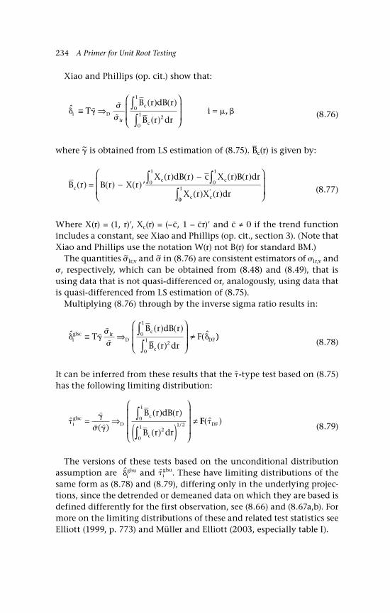
234 A Primer for Unit Root Testing
Xiao and Phillips (op. cit.) show that:
ˆ( ) ( )
( ),
i D
lr
c
c
TB r dB r
B r dri≡ ⇒
=∫∫0
1
2
0
1
(8.76)
where ~ is obtained from LS estimation of (8.75). B–c(r) is given by:
B r B r X rX r dB r c X r B r dr
X r X r drc
c c
c c
( ) ( ) ( )’( ) ( ) ( ) ( )
( ) ( )’= −
−∫ ∫0
1
0
1
00
1
∫
(8.77)
Where X(r) = (1, r), Xc(r) = (–c–, 1 – c–r) and c– ≠ 0 if the trend function includes a constant, see Xiao and Phillips (op. cit., section 3). (Note that Xiao and Phillips use the notation W(r) not B(r) for standard BM.)
The quantities ~lr,v and ~ in (8.76) are consistent estimators of lr,v and , respectively, which can be obtained from (8.48) and (8.49), that is using data that is not quasi-differenced or, analogously, using data that is quasi-differenced from LS estimation of (8.75).
Multiplying (8.76) through by the inverse sigma ratio results in:
ˆ( ) ( )
( )( ˆ
i
glsc lrD
c
c
DFTB r dB r
B r drF≡ ⇒
≠∫∫0
1
2
0
1 ))
(8.78)
It can be inferred from these results that the -type test based on (8.75) has the following limiting distribution:
ˆ( )
( ) ( )
( )/
iglsc
D
c
c
B r dB r
B r dr= ⇒
( )
≠∫∫
0
1
2
0
1 1 2 FF DF(ˆ )
(8.79)
The versions of these tests based on the unconditional distribution assumption are i
glsu and iglsu. These have limiting distributions of the
same form as (8.78) and (8.79), differing only in the underlying projec-tions, since the detrended or demeaned data on which they are based is defined differently for the first observation, see (8.66) and (8.67a,b). For more on the limiting distributions of these and related test statistics see Elliott (1999, p. 773) and Müller and Elliott (2003, especially table I).
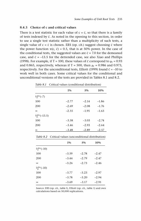
Some Examples of Unit Root Tests 235
8.4.3 Choice of c and critical values
There is a test statistic for each value of c = c–, so that there is a family of tests indexed by c–. As noted in the opening to this section, in order to use a single test statistic rather than a multiplicity of such tests, a single value of c = c– is chosen. ERS (op. cit.) suggest choosing c– where the power function (c, c–) = 0.5, that is at 50% power. In the case of the conditional tests, the suggested values are c– = 7.0 for the demeaned case, and c– = –13.5 for the detrended case, see also Xiao and Phillips (1998). For example, if T = 100, these values of c– correspond to c– = 0.93 and 0.865, respectively, whereas if T = 500, then c– = 0.986 and 0.973, respectively. For the unconditional tests, Elliott (1999) found c– = –10 to work well in both cases. Some critical values for the conditional and unconditional versions of the tests are provided in Tables 8.1 and 8.2.
Table 8.2 Critical values (unconditional distribution)
1% 5% 10%
glsc(–10)
100 –3.59 –2.78 –2.47
200 –3.44 –2.79 –2.47
∞ –3.26 –2.73 –2.46
glsc(–10)
100 –3.77 –3.23 –2.97
200 –3.78 –3.20 –2.94
∞ –3.69 –3.17 –2.91
Sources: ERS (op. cit., table I), Elliott (op. cit., table 1) and own calculations based on 50,000 replications.
Table 8.1 Critical values (conditional distribution)
1% 5% 10%
glsc(–7)
100 –2.77 –2.14 –1.86
200 –2.69 –2.08 –1.76
∞ –2.55 –1.95 –1.63
glsc(–13.5)
100 –3.58 –3.03 –2.74
200 –3.46 –2.93 –2.64
∞ –3.48 –2.89 –2.57

236 A Primer for Unit Root Testing
8.4.4 Power of ERS-type tests
To illustrate the potential gains in power, Figures 8.9–8.12 summarise the results from 5,000 simulations with T = 100. In each case the DGP is yt = yt–1 + t, where t ~ N(0, 1); = 1 corresponds to the null hypothesis and < 1 to the alternative hypothesis. The simulated power function records the proportion of correct decisions to reject the null hypothesis when carrying out a unit root test at the 5% significance level.
The comparisons are illustrated as follows: and glsc in Figure 8.9;
and glsc in Figure 8.10; and
glsu in Figure 8.11; and and glsu in
Figure 8.12. The power functions using efficiently detrended data lie above those for the standard DF tests for both variants. For example, in the case of the conditional distribution assumption, power at = 0.85 is 62% for and 93% for
glsc, and 41% for and 58% for glsc; when the
initial draw is from the unconditional distribution, the powers are 62% for and 72% for
glsu, and 40% for and 49% for glsu. Notice that on
a pairwise basis for glsc and
glsu, and glsc and
glsu, power is greater for the conditional distribution assumption.
These simulations suggest that the initial condition may be influential in determining the power of a unit root test and, indeed, this is the case;
0.65 0.7 0.75 0.8 0.85 0.9 0.95 10
0.1
0.2
0.3
0.4
0.5
0.6
0.7
0.8
0.9
1
initial draw: conditional distribution
µglsc
µ
93%
62%τ
τ
Figure 8.9 Comparison of power, glsc, (demeaned) T = 100
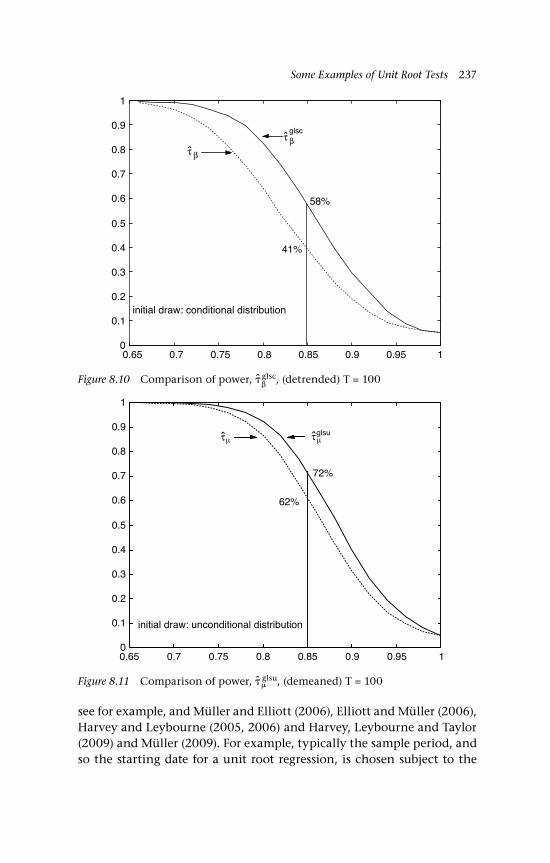
Some Examples of Unit Root Tests 237
0.65 0.7 0.75 0.8 0.85 0.9 0.95 10
0.1
0.2
0.3
0.4
0.5
0.6
0.7
0.8
0.9
1
initial draw: conditional distribution
58%
41%
βglsc
τ βτ
Figure 8.10 Comparison of power, glsc, (detrended) T = 100
0.65 0.7 0.75 0.8 0.85 0.9 0.95 10
0.1
0.2
0.3
0.4
0.5
0.6
0.7
0.8
0.9
1
initial draw: unconditional distribution
µglsu
µ
62%
72%
ττ
Figure 8.11 Comparison of power, glsu, (demeaned) T = 100
see for example, and Müller and Elliott (2006), Elliott and Müller (2006), Harvey and Leybourne (2005, 2006) and Harvey, Leybourne and Taylor (2009) and Müller (2009). For example, typically the sample period, and so the starting date for a unit root regression, is chosen subject to the
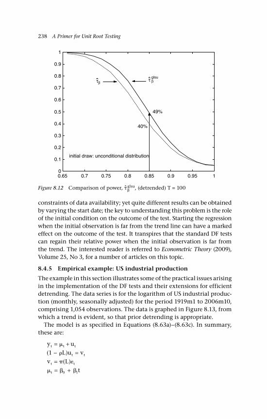
238 A Primer for Unit Root Testing
constraints of data availability; yet quite different results can be obtained by varying the start date; the key to understanding this problem is the role of the initial condition on the outcome of the test. Starting the regression when the initial observation is far from the trend line can have a marked effect on the outcome of the test. It transpires that the standard DF tests can regain their relative power when the initial observation is far from the trend. The interested reader is referred to Econometric Theory (2009), Volume 25, No 3, for a number of articles on this topic.
8.4.5 Empirical example: US industrial production
The example in this section illustrates some of the practical issues arising in the implementation of the DF tests and their extensions for efficient detrending. The data series is for the logarithm of US industrial produc-tion (monthly, seasonally adjusted) for the period 1919m1 to 2006m10, comprising 1,054 observations. The data is graphed in Figure 8.13, from which a trend is evident, so that prior detrending is appropriate.
The model is as specified in Equations (8.63a)–(8.63c). In summary, these are:
y u
L u v
v L
t
t t t
t t
t t
t
= +− === +
( )
( )
1
0 1
0.65 0.7 0.75 0.8 0.85 0.9 0.95 10
0.1
0.2
0.3
0.4
0.5
0.6
0.7
0.8
0.9
1
βglsu
β
49%
40%
initial draw: unconditional distribution
ττ
Figure 8.12 Comparison of power, glsu, (detrended) T = 100

Some Examples of Unit Root Tests 239
1920 1930 1940 1950 1960 1970 1980 1990 20001
1.5
2
2.5
3
3.5
4
4.5
5L
og
s
Figure 8.13 US industrial production (logs, p.a, s.a)
Together these imply an ADF model of the following general form (see Equation (8.75)):
ˆ ˆ ˆ,y y c yt t jj
p
t j t p= + +− =
−−∑ 1 1
1
where ˆ ˆ ( ˆ ˆ )y y y tt t t t= − = − + 0 1 . In the case of ‘efficient’ detrending, y~t is replaced by y~c,t where detrending is based on either the conditional or unconditional assumption for the initial draw, referred to as GLSC and GLSU, respectively.
The detrending results are summarised in Table 8.3 and the ADF test results are reported in Table 8.4. The order, p*, of the ADF regression was chosen by a general-to-specific search using the marginal t crite-rion, that is the longest lag was omitted if its estimated coefficient was not significant at the % two-sided significance level. The maximum lag was set at 20 and % was set equal to 1% to avoid unwanted accu-mulation of type I error. This resulted in a lag length of 14 for the ADF model, where the marginal t statistic had a p-value of less than 0.5%.
The values of the test statistics differ only marginally. None of the
–type tests lead to rejection of the null hypothesis of a unit root at the 5% significance level but, because the limiting null distributions differ,

240 A Primer for Unit Root Testing
the implied p-values of each test value do differ, with p-values decreas-ing in order for ,
glsu then glsc . For example, using a 10% significance
level leads to rejection with glsc, but not with or
glsu. The tests are also reported in Table 8.4. Using and
glsu leads to the same conclusion
as using their pseudo-t counterparts. Whilst using glsc
leads to rejection of the null hypothesis at the 5% significance level, it is probably the case that of the two GLS-type tests, this is the less preferred.
It is known that these test statistics can be sensitive to the initial observation and, as is evident from Figure 8.13, there are some sub-stantial deviations from trend. For example, the observations around 1932/33 are a long way from trend, as could be expected from the onset of the Great Crash, and the test statistics start to differ quite noticeably from 1929 onward. For example, if the starting date of the test regres-sion is taken to be 1933m1, then the test statistics do give quite differ-ent results. These are summarised in Table 8.5, where it is now the case that whilst the DF versions of the test statistics are almost unchanged, the test value of
glsc becomes less negative as does glsu, but less so,
which, ceteris paribus, would be taken as evidence not to reject the null hypothesis. There are a number of ways around this sensitivity, for example by forming a weighted test statistic, see Harvey and Leybourne
Table 8.4 Unit root test statistics from ADF(14) maintained regression
DF GLSC GLSU
–0.0108 –0.0103 –0.0104
-type test = –2.737 glsc = –2.687
glsu = –2.703
ˆ ˆ( ˆ( ))
=
−T
c1 1ˆ .
( . )
.
= −−
= −
11 261 0 424
19 54
ˆ .( . )
.
glsc = −
−= −
10 731 0 419
18 47
ˆ .( . )
.
glsu = −
−= −
10 801 0 419
18 61
Notes: 5% (10%) critical values, : –3.41 (–3.13); glsc: –2.89 (–2.57);
glsu: –3.17 (–2.91);
: –21.7 (–18.3); glsc: –16.53 (–13.49);
glsu: –19.79 (–16.17).
Table 8.3 Estimation of trend coefficients: LS and ‘efficient’ detrending
LS GLSC, c– = –13.5 GLSU, c– = –10.0
0 1.614 1.682 1.666
1 0.00315 0.00303 0.00302
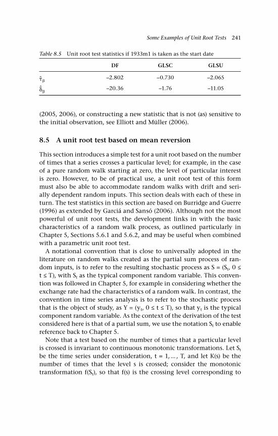
Some Examples of Unit Root Tests 241
(2005, 2006), or constructing a new statistic that is not (as) sensitive to the initial observation, see Elliott and Müller (2006).
8.5 A unit root test based on mean reversion
This section introduces a simple test for a unit root based on the number of times that a series crosses a particular level; for example, in the case of a pure random walk starting at zero, the level of particular interest is zero. However, to be of practical use, a unit root test of this form must also be able to accommodate random walks with drift and seri-ally dependent random inputs. This section deals with each of these in turn. The test statistics in this section are based on Burridge and Guerre (1996) as extended by Garciá and Sansó (2006). Although not the most powerful of unit root tests, the development links in with the basic characteristics of a random walk process, as outlined particularly in Chapter 5, Sections 5.6.1 and 5.6.2, and may be useful when combined with a parametric unit root test.
A notational convention that is close to universally adopted in the literature on random walks created as the partial sum process of ran-dom inputs, is to refer to the resulting stochastic process as S = (St, 0 ≤ t ≤ T), with St as the typical component random variable. This conven-tion was followed in Chapter 5, for example in considering whether the exchange rate had the characteristics of a random walk. In contrast, the convention in time series analysis is to refer to the stochastic process that is the object of study, as Y = (yt, 0 ≤ t ≤ T), so that yt is the typical component random variable. As the context of the derivation of the test considered here is that of a partial sum, we use the notation St to enable reference back to Chapter 5.
Note that a test based on the number of times that a particular level is crossed is invariant to continuous monotonic transformations. Let St be the time series under consideration, t = 1, ... , T, and let K(s) be the number of times that the level s is crossed; consider the monotonic transformation f(St), so that f(s) is the crossing level corresponding to
Table 8.5 Unit root test statistics if 1933m1 is taken as the start date
DF GLSC GLSU
–2.802 –0.730 –2.065
–20.36 –1.76 –11.05
242 A Primer for Unit Root Testing
the transformed variable, then the number of times that f(St) crosses f(s) is also K(s). This feature has a constructive and a nonconstructive aspect. For example, suppose that we are unsure whether to test for mean reversion in the log or the level of a series. If a standard DF test is used, different results will be produced if lnSt and St are used. This will not be the case for a test based on K(s), so non-rejection is non-rejection for all monotonic transformations; but this does not tell us for which transformation (including no transformation) the unit root exists. To determine that question, other tests are needed.
8.5.1 No drift in the random walk
In this case, the random walk is of the form given by the partial sum process St = St–1 + t, t ≥ 1, where tT
t=1 is a sequence of continuous ran-dom variables distributed as iid(0, 2). S0 and 1 are assumed to be ran-dom variables with bounded pdfs and finite variance; thus, the often assumed starting assumption S0 = 0 is permitted, interpreting S0 as a degenerate random variable. (Also the boundedness condition can be relaxed, see Burridge and Guerre, op. cit., Remark 1.)
The first problem is to determine the distribution of a test statistic based on the number of level crossings under the null that the data generating process was a simple random walk. The number of crossings of the level s, normalised by T , is:
K s T I S s S s I S s S sT tt
T
t t t( ) [ ( , ) ( , )]/= ≤ > + > ≤( )−−= −∑1 2
11 1
(8.82)
where I(.) is the indicator function, equal to 1 if the condition is true and 0 otherwise. The first part of the condition (8.82) captures the case when the level s is crossed from below and the second part of the condi-tion captures the case when the level s is crossed from above. Burridge and Guerre (1996, Theorem 1), show for any s, then KT(s):
K sE
z zT D( )| |
| | | |⇒ =1
'
(8.83)
where ' = E |1|/ and z is a random variable distributed as standard nor-mal, z ~ N(0, 1). It follows that:
K s K s zT T D* ( ) ( ) | |≡ ⇒−' 1
(8.84)

Some Examples of Unit Root Tests 243
In distributional terms this is stated as:
F K s zT D[ ( )] (| |)* ⇒ (8.85)
where F[K*T(s)] is the distribution function of K*
T(s) and (|z|) is the half-normal distribution function, which is a special case of the folded normal distribution. It is the distribution of the absolute value of a nor-mally distributed random variable with mean zero and variance 2 = 1. It ‘folds’ over the left-side of the normal pdf onto the right hand side. Typically we are interested in tail probabilities, for example in deter-mining 1 – (| z |) = for a given value of z or finding z for a given value of . This procedure is familiar from (z); for example, 1 – (1.96) = 0.025. In the case of (|1.96|), the right tail probability is 1 – (|1.96|) = 2(1 – (1.96)) = 0.05, and the tail probability is doubled for a given value of . The generalisation of this result is 1 – (| z |) = 2(1 – (z)) ⇒ (| z |) = 2(z) – 1.
Replacing the unknown quantities and E | 1 | by consistent estimators will not alter the limiting distribution. The suggested estimators are:
ˆ //
= ( ) →−=∑T Stt
T
p1 2 2
1
1 2
(8.86)
ˆ | | | | | |E T S Ett
T
p 11
1 1= →−=∑
(8.87)
These are obtained noting that under the null hypothesis t = St, and by the iid assumption E|1| = E|t|, t = 2, ... , T; hence, the estimator of E| 1 | is based on all T observations on St. The estimator E | 1 | is the (sample) mean absolute deviation (MAD) and the resulting test statistic, denoted (0) for simplicity, is:
( )
| |( ) | |0
1
≡ ⇒ˆE
K s zT D
(8.88)
In practice, a value for the level s is chosen, the test statistic is cal-culated and compared to the upper quantiles of (| z |). In the case of a pure random walk starting at zero, the level s = 0 is chosen, so that the test statistic is interpreted as a test of mean reversion. Under the alternative hypothesis of stationarity, the test statistic diverges because the number of changes of sign increases; therefore, large values of (0) relative to the (1 – α)% quantile of (| z |) lead to rejection of the null

244 A Primer for Unit Root Testing
hypothesis of a unit root at the α significance level. Some finite sample critical values are provided by Burridge and Guerre (op. cit., table 1) and García and Sansó (op. cit., table 1); and see Table 8.6 below.
This distribution (| z |) = 2(z) – 1, has been encountered before in Chapter 5, as the distribution of the normalised number of mean rever-sions for a symmetric binomial random walk (see Chapter 5, Equation 5.15 in Section 5.6.1). Thus, although it has been assumed here that the t are continuous random variables, the distributional result in (8.85) also holds for t = –1, +1) with probability ½ for each outcome; then = 1 and E|1| = 1, hence F[KB,T(0)] ⇒D |(| z |), which is the result in Equation (5.15); (recall that the B subscript indicates binomial inputs). This also accounts for the difference in the number of mean reversions when the symmetric random walk is alternately specified with Gaussian inputs and –1, +1) inputs – a difference that was noted in Chapter 5, Table 5.2 (see Section 5.6.2). First note that the Cauchy-Schwarz inequality implies that '–1 = /E | 1 | ! 1, see Burridge and Guerre (op. cit., Remark 2, in the form that 0 ≤ ' ≤ 1); then ' − =1 1 2E K sT[ ( )] / implies that E[KT(s)] ≤ E[KB,T(s)]; the mean number of reversions with continuous iid random variables is no greater than with binomial inputs. (Note that ' is a constant and the mean of a random variable distributed as half (standard) normal is 2/, see Section 5.6.2.)
8.5.2 Drifted random walk
In the case of a drifted random walk, St = + St–1 + t = t + S0 + S~t, where St jj
t=
=∑ 1
. The deterministic trend in this series is t, which will tend to impart a direction, or drift, to the random walk generated by the stochastic trend S~t (for examples of drift, see Chapter 5, Section 5.4.2, Figure 5.7). This is why if a random walk is an appropriate model for aggregate macroeconomic time series, such as GDP and consump-tion expenditure, then it should contain a drift parameter. However, the presence of a direction to the time series will confuse the previous test for level crossings (mean reversion). For example, a series that is sta-tionary around a positive trend, will not generate systematic crossings of any particular level, so the test statistic, K*T(s), which was designed for the random walk without a drift, will not be able to discriminate in favour of the alternative.
What we need to consider is S~t, interpreted as a detrended random walk, rather than St. In order to achieve this note that:
S
S S
t jj
t
t t
=
= − +=∑ 1
0( ) (8.89)
Some Examples of Unit Root Tests 245
So that what is required is an estimator of , say , so that the trend component can be removed from St, that is:
ˆ ( ˆ )S t + St 0= −St (8.90)
Note that = St + t, so that a consistent estimator of is provided by:
ˆ
( )
=
= −
−=
−
∑T S
T S S
tt
T
T
1
1
10
(8.91)
St is an estimator of the I(1) component jj
t
=∑ 1, just as in the case with-
out drift. The test statistic is derived in the same way replacing St by St, so that the first step is to obtain the normalised number of sign changes:
K s T I s s s sT tt
Tt t t( ) [ ( , ) ( , )]/= ≤ > + > ≤
−
−= −∑1 21
11S S S S
ˆ ˆ ˆ ˆ
(8.92)
The test statistic is:
( )
| |( )1
1
= ⇒ˆE
K s RT D
(8.93)
where
=
−=∑T t
t
T1 2 2
1
1 2
/
/
Sˆ
E T tt
T| | | |1
1
1= −
=∑ Sˆ
R is a random variable with the standard Rayleigh distribution; the density function is f x I x x xR( ) ( ) exp( )= > −0 1
22 , where I(.) is the indicator function
taking the value 1 when x > 0 and 0 otherwise. Some critical values for (0) and (1) are given in Table 8.6, with more extensive tabulations in Burridge and Guerre (op. cit., table 1) and García and Sansó (op. cit., table 1).
8.5.3 Serial dependence
So far it has been assumed that stochastic input to the partial sum process denoted t, was not serially dependent; however, as this is not often the case, the method must be able to deal with serially dependent inputs (referred to as ‘errors’). To accommodate this possibility consider the random walk model, but with serially dependent errors, denoted by

246 A Primer for Unit Root Testing
ut (to distinguish them from t):
S S ut t t= +−1 (8.94)
u
L
t jj t j
t
=
==
∞−∑
0
( )
(8.95)
where t ~ iid(0, 2) and E| t |r for some r > 2; also, 0 = 1, (1) ≠ 0 and j jj| |
=
∞∑ < ∞0
, see García and Sansó (op. cit.). The moving average speci-fication of ut is familiar from Chapter 2, see Section 2.6, from which we note that the long-run variance of ut = St is lr,S = (1)22. For example, if ut = &ut–1 + t, then lr,S = (1 – &2)–12; see also Section 8.3.2. If the ran-dom walk has a drift component, as in Section 8.5.2, then St is detrended to obtain S
~t and the required long-run variance is denoted lr,S
~.The solution to the problem of serial dependence in the errors is now
simple (and may now be recognised as following a general principle) and just involves replacing in (0)
or (1), as the case may be, by the respective long-run standard error; that is lr,S, for St, and lr,S
~ for St. The sample value of the test statistic then uses a consistent estima-tor obtained, for example, by a semi-parametric method or an autore-gressive estimator as illustrated in Chapter 2, see Sections 2.5 and 2.6. The revised test statistics are:
lrlr S
T DE u
K s z( ) ,
| |( ) (| |)0
1
= ⇒ˆ
ˆ
(8.96)
Table 8.6 Critical values for the levels crossing test statistics, (0) and (1)
(0) (1)
90% 95% 90% 95%
100 1.52 1.82 2.07 2.36
200 1.56 1.85 2.08 2.38
500 1.60 1.91 2.11 2.40
1,000 1.61 1.91 2.12 2.41
∞ 1.645 1.96 2.14 2.44
Note: Source, García and Sansó (op. cit., table 1).
Some Examples of Unit Root Tests 247
lrlr S
T DE uK s R( ) ,
| |( )1
1
= ⇒
(8.97)
where ˆ | | | |E u T Stt
T
11
1= −
=∑ for lr( )0 and T
t
T−=∑1
1| |St
ˆ for (1)
lr; otherwise, compared to (0) and (1), 1 and ~ have been replaced by lr and ~lr, respectively. Note that the asymptotic distributions are unchanged.
In some illustrative simulation results, with an MA(1) generating process ut = (1 + 1L)t, Garcia and Sanso (op. cit.) find that whilst (1)
lr is not as powerful as glsc, it maintains its size better especially in the
problematic case when 1 → – 1.
8.5.4 Example: Gold-silver prices
This example continues that in Chapter 5, Section 5.8.2, which used a sample of 5,372 observations on the log ratio of gold to silver prices, which is the variable St in this case. The price ratio was normalised to unity at the beginning of the sample implying that the log ratio was normalised at zero. The graph of the data does not reveal any evidence of drift in the ratio (see Figure 5.17), so the test statistic (0) (or lr
( )0 ) is preferred. As previously noted, the number of sign changes in the sam-ple of 5,372 observations was only 32, so there is strong presumption of a random walk. The expected number of sign changes for a random walk with N(0, 2) inputs is 46.6. The likelihood of random walk is strongly suggested by the sample value of the test statistic calculated as follows:
( )
( ) | |( )
.
. ,
.
0
1
21
0 01380 0094
325 372
0 64
=−
= ×
=
−=∑
ˆ
T SK s
tt
T T
This value is well below the 95% quantile of 1.96; indeed, the p-value of 0.64 is 0.52.
To take into account the possibility of serial dependence, the long-run variance of ut = St was estimated by the two methods outlined in Chapter 2, Sections 2.6.1 and 2.6.2. The first of these is semi-par-ametric, with two estimators depending upon whether a kernel esti-mator is used. To illustrate the difference it makes to the estimates, the unweighted and Newey-West estimates of 2
lr,S are graphed in
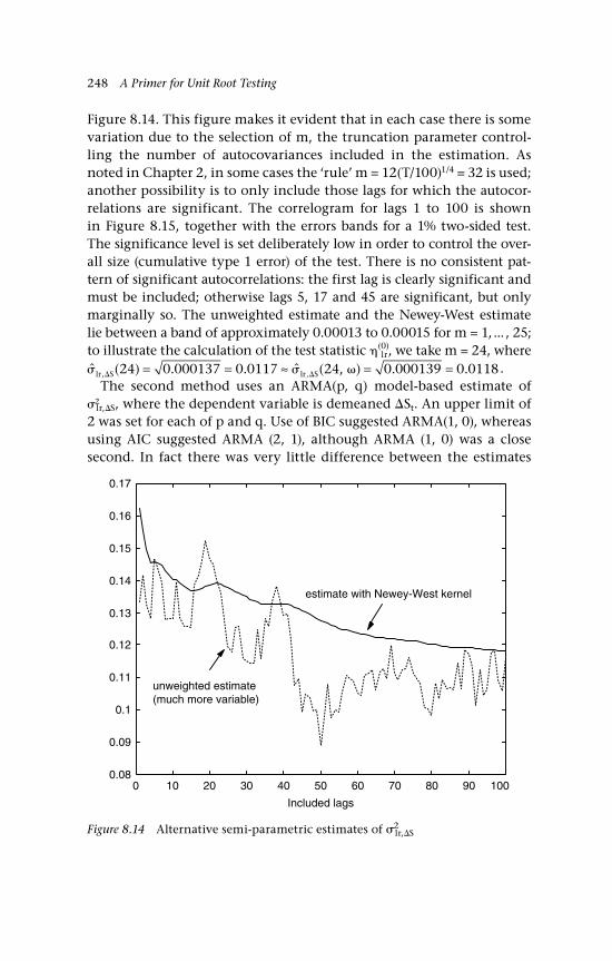
248 A Primer for Unit Root Testing
Figure 8.14. This figure makes it evident that in each case there is some variation due to the selection of m, the truncation parameter control-ling the number of autocovariances included in the estimation. As noted in Chapter 2, in some cases the ‘rule’ m = 12(T/100)1/4 = 32 is used; another possibility is to only include those lags for which the autocor-relations are significant. The correlogram for lags 1 to 100 is shown in Figure 8.15, together with the errors bands for a 1% two-sided test. The significance level is set deliberately low in order to control the over-all size (cumulative type 1 error) of the test. There is no consistent pat-tern of significant autocorrelations: the first lag is clearly significant and must be included; otherwise lags 5, 17 and 45 are significant, but only marginally so. The unweighted estimate and the Newey-West estimate lie between a band of approximately 0.00013 to 0.00015 for m = 1, ... , 25; to illustrate the calculation of the test statistic (0)
lr, we take m = 24, where ˆ ( ) . . ˆ ( , ) . ., , lr S lr S24 0 000137 0 0117 24 0 000139 0 0118= = ≈ = = .
The second method uses an ARMA(p, q) model-based estimate of 2
lr,S, where the dependent variable is demeaned St. An upper limit of 2 was set for each of p and q. Use of BIC suggested ARMA(1, 0), whereas using AIC suggested ARMA (2, 1), although ARMA (1, 0) was a close second. In fact there was very little difference between the estimates
0 10 20 30 40 50 60 70 80 90 1000.08
0.09
0.1
0.11
0.12
0.13
0.14
0.15
0.16
0.17
estimate with Newey-West kernel
unweighted estimate(much more variable)
Included lags
Figure 8.14 Alternative semi-parametric estimates of 2lr,S
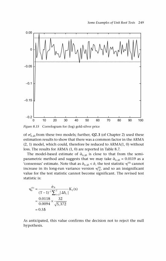
Some Examples of Unit Root Tests 249
of 2lr,S from these two models; further, Q2.3 (of Chapter 2) used these
estimation results to show that there was a common factor in the ARMA (2, 1) model, which could, therefore be reduced to ARMA(1, 0) without loss. The results for ARMA (1, 0) are reported in Table 8.7.
The model-based estimate of lr,S is close to that from the semi-parametric method and suggests that we may take lr,S = 0.0119 as a ‘consensus’ estimate. Note that as lr,S < , the test statistic (0) cannot increase in its long-run variance version (0)
lr, and so an insignificant value for the test statistic cannot become significant. The revised test statistic is:
lrlr
tt
T TT S
K s( )
( ) | |( )
.
. ,
.
0
1
21
0 01180 0094
325 372
0 5
=−
= ×
=
−=∑
ˆ
55
As anticipated, this value confirms the decision not to reject the null hypothesis.
Figure 8.15 Correlogram for (log) gold-silver price
0 10 20 30 40 50 60 70 80 90 100−0.2
−0.15
−0.1
−0.05
0
0.05

250 A Primer for Unit Root Testing
8.6 Concluding remarks
Tests for a unit root are in widespread use primarily for two reasons. First, the question of whether a time series has been generated by a process that has this form of nonstationarity is of interest in its own right with, for example, implications for the persistence of shocks and the existence or otherwise of an equilibrium to which a series will revert in the long run. Second, the concept of cointegration, which involves jointly modelling several series, is concerned with whether integrated series are related, as suggested in particular cases by eco-nomic theory.
This chapter has been but a ‘dip’ into some of the existing tests. Some interesting problems that arise in the theoretical and applied literature of unit root testing include the following.
1. The treatment of the initial observation under the alternative is critical, as is the specification of the deterministic components; see, for example, Harvey, Leybourne and Taylor (2009), and the refer-ences and series of comments on that article in Econometric Theory (2009).
2. MA errors can lead to near cancellation of unit roots, which can cause severe size distortions (oversizing) in unit root tests; hence, in the limit is it possible to discriminate between stationary and non-stationary processes? See Schwert (1987) and Müller (2008).
3. Breaks in time series, which are in a stationary in pieces (‘piecewise stationarity’) that is between the breaks, can look like series generated by a unit root nonstationary process. The seminal article on this topic is Perron (1989), which has led to a considerable literature on break detection see, for example, Perron (2006) for a critical overview.
Table 8.7 ARMA model-based estimates
1 2lr,S and lr,S
ARMA(1, 0) –0.152(–11.28)
0.0137ˆ ( ) ˆ
( ( . ))ˆ
.
ˆ .
,
,
lr S
lr S
w
2 2 22
211
1 0 152
0 000141
0 0001
= =− −
=
= 441 0 0119= .
Notes: t statistic in parentheses; dependent variable, St S− where ˆ ( ) S tt
TT S= − −
=∑1 1
2

Some Examples of Unit Root Tests 251
4. Autoregressive processes that are ‘triggered’ by a variable that exceeds a threshold value and which may have a unit root, referred to as threshold autoregressive (TAR) models, have also been of theo-retical and empirical interest see, for example, Caner and Hansen (2001), Van Dijk, Teräsvirta and Franses (2002), Strikholm and Teräsvirta (2004), Lundbergh, Teräsvirta, and Dijk. (2003) and for an overview of nonlinear TAR models see Teräsvirta (2006).
5. A time series ‘contaminated’ by outliers can also be confused with one generated by a unit root nonstationary process see, for exam-ple, Franses and Haldrup (1994), Harvey and Leybourne (2001) and Popp (2008).
6. There is empirical evidence that a time series may become station-ary after applying the fractional differencing operator (1 – L)d, where d is not an integer, thus restricting d to be an integer is a form of misspecification; for an overview of this concept and tests, see Gil-Alana and Hualde (2009).
7. Bounded variables: many economic time series are bounded, for example the nominal interest rate, unemployment and variables constructed as shares, such as the components of wealth relative to total wealth; however, random walks are necessarily unbounded. Can processes be constructed that generate random walks that are bounded? See, for example, Cavaliere (2002).
8. Will differencing a nonstationary series necessarily reduce it to stationarity? Clearly this will not always be the case. Such cases are of empirical interest and have been modelled as stochastic unit roots. See, for example, Leybourne, McCabe and Tremayne (1996), Granger and Swanson (1997), Leybourne, McCabe and Mills (1996) and Taylor and Van Dijk (2002).
9. Detecting more than one unit root may be a critical issue for some time series, such as those, like prices and wages, in nominal terms. What happens if the possibility of a second root is left undetected? Is the best test for two unit roots, the same as the one unit root test applied to the first difference of the series? See for example Haldrup and Lildholdt (2002), Haldrup and Jansson (2006) and Rodrigues and Taylor (2004).
10. Many time series have a seasonal pattern and the question then is whether the seasonally adjusted or the unadjusted series should be used in order to test for a unit root. For a consideration of the issues and references see Fok, Franses and Paap (2006) and for some test statistics applied to seasonally unadjusted series see, for example, Osborn and Rodrigues (2002) and Rodrigues and Taylor (2004a,b).
252 A Primer for Unit Root Testing
Questions
Q8.1 Consider the demeaned AR(1) model given by (8.17), as follows:
y yt t t− = − +− ( )1 (A8.1 = 8.17)
Suggest a method of demeaning the data such that the estimate of and its t statistic are identical to those obtained from estimation with an explicit constant:
y yt t t= + +− * 1 (A8.2 = 8.28)
A8.1 Demean yt and yt–1 separately, that is estimate:
y y y yt t t− = − +− −0 1 1 ( ) (A8.3)
where y y Ttt
T
0 21= −
=∑ /( ) and y y Ttt
T
− =
−= −∑1 1
11/( ); this ensures that the
regressand and the regressor are identical under both methods and, hence, the estimators of will be the same. Next, to ensure that the estimated standard errors of are also identical, either compute the estimated standard error from (A8.3) as the square root of the residual sum of squares divided by (T – 2), hence making an adjustment for implicit estimation of the mean, as in the LS estimator from (A8.2); or divide each residual sum of squares by (T – 1). Either way, the resulting standard errors will be the same and so will the t statistics calculated using these standard errors.
Q8.2 Given the results of Q7.2 that T y W r drtt
T
D−
−=∑ ∫⇒21
2
1
2
0
1( ) and
T y W r dW rt t D−
−∑ ∫⇒11 0
1 ( ) ( ), confirm the following:
ˆ ( ˆ )( )
( )
≡ − ⇒
−( )∫
TB r dr
D112
1 12
2
0
1
A8.2 From Table 7.1, we have the following:
T y W r dr B r dr
T y B
tt
T
D
t t D
−−=
−−
∑ ∫ ∫∑
⇒ =
⇒
21
2
1
2
0
1 2 2
0
1
11
212
1
( ) ( )
( )
−−( ) −( )112
1 12 2~ ( )
Some Examples of Unit Root Tests 253
The test statistic is:
ˆ /
/ = −=
−=
∑∑
y T
y T
t tt
T
tt
T
11
12
1
2
The convergence results for the numerator and denominator together with the extended CMT imply that:
TB r dr B r
D( )( )
( )
( )
( )
ˆ − ⇒
−( )=
−( )∫
1
12
1 1 12
1 12 2
2 2
0
1
2
22
0
1dr∫
See Davidson (1994) for some expansion of this and related results.
Q8.3 Interpret the following model under the null hypothesis H0 : = 1 and compare it with the interpretation under the alternative hypothesis HA : < 1.
y u
L u v
v
t
t t t
t t
t t
t
= +− === +
( )1
0 1
A8.3 First obtain the reduced form by substituting ut and then t into the second equation:
( ) ( )y yt t t t t− = − +− − 1 1
y t y
t y
t t t
t t
= − + + − + +
= + + +−
−
0 1 1 1
0 1 1
1 1( ) ( )
* *
where *0 = 0 (1 – ) + 1 and *
1 = 1(1 – ). Provided that these restric-tions are used then = 1 implies that yt = 1 + t, so that 1 is the drift under H0 and the invariance of the test regression to the unknown value of 1 is ensured by prior detrending (or directly including a trend in the maintained regression). Under < 1, there are stationary deviations from the linear trend t = 0 + 1t, to which observations will revert if there are no shocks. With no further dynamics in the structural equa-tions, shocks die out geometrically.

254 A Primer for Unit Root Testing
Appendix: Response functions for DF tests and
The form of the response functions follows MacKinnon (1991), as extended by Cheung and Lai (1995a, b) and Patterson and Heravi (2003). The general notation is Cj(ts, , T, p*), which is the estimate of the α percentile of the distribution of test statistic ts, for T and p* = k – 1; ‘observations’ are indexed by j = 1, ..., N; and T ≡ T – p adjusts for the actual sample size. The general form of Cj(ts, , T, p*) is:
C ts T p T p Tj ii
i
I
jj
j
J
j( , , , *) / ( * / ) ' ' = + + +∞= =∑ ∑
1 1 (A8.1)
A factorial experimental design was used over all different pairings of T and p*, with p* = 0, 1, ..., 12. The sample size T and the increments (in parentheses) were then as follows: T = 20(1), 51(3), 78(5), 148(10), 258(50), 308(100), 508(200), 908. In all there were 66 × 13 = 858 sample points from which to determine the response functions for the 1st, 5th and 10th percentiles. The coefficient ' gives an approximate guide as to the critical value for large T.
The tables are arranged in three parts distinguished by the specifi-cation of the trend function, with t = 0, t = and t = 0 + 1t. As an example of their use consider estimating a maintained regression with t = , T = 100 and p* = 4 then the 5% critical value for is obtained as:
C Tj( , . , , )
. ( . / ) ( . / )
. ( /
0 05 4
2 863 3 080 100 5 977 100
0 902 4
2= − − − +
1100 1 470 4 100 1 527 4 100
2 861
2 3) . ( / ) . ( / )
.
− += −
In fact, the asymptotic 5% critical value provides quite a good ‘eyeball’ figure for T > 50, but the differences are more noticeable with the ver-sions of the tests.

Tabl
e A
8.1
1%, 5
% a
nd
10
% c
riti
cal
valu
es f
or
t = 0
No
co
nst
ant
and
no
tre
nd
Co
effi
cien
ts f
or 1
% c
riti
cal
valu
es
Test
s'
' 1
' 2' 3
1
2
3
R2
−2
.559
9−3
.039
28
−33.
3711
106.
5659
1.2
04
48−2
.394
152
.499
499
0.91
4757
−1
3.53
09
117.
8137
−790
.263
28
08.
642
−18.
1035
9.31
2984
−57.
3207
0.98
401
2
Co
effi
cien
ts f
or 5
% c
riti
cal
valu
es
Test
s'
' 1
' 2' 3
1
2
3
R2
−1
.938
93−
0.49
021
−30.
6711
145.
407
20.
8398
98−1
.210
310.
7222
830.
8963
97
−7
.946
9368
.476
36−
494.
355
1619
.858
−6.
206
340.
1268
17−2
1.06
830.
9802
75
Co
effi
cien
ts f
or 1
0%
cri
tica
l va
lues
Test
s'
' 1
' 2' 3
1
2
3
R2
−1
.615
810.
0261
71−2
2.5
668
108.
9953
0.69
6141
−0.
9471
50.
4797
64
0.92
1401
−5
.658
7650
.452
6−3
91.6
24
1287
.258
−3.1
8757
−1.0
887
−12
.541
60.
9823
63

Tabl
e A
8.2
1%, 5
% a
nd
10
% c
riti
cal
valu
es f
or
t =
Co
nst
ant,
no
tre
nd
Co
effi
cien
ts f
or 1
% c
riti
cal
valu
es
Test
s'
' 1
' 2' 3
1
2
3
R2
−3
.429
82−7
.219
8−4
.111
−143
.64
1.14
6321
−2.3
9972
3.06
403
70.
9719
63
−2
0.45
7656
.067
3610
45.5
66−9
727.
2−5
3.71
9513
.441
47−1
74.1
90.
9984
22
Co
effi
cien
ts f
or 5
% c
riti
cal
valu
es
Test
s'
' 1
' 2' 3
1
2
3
R2
−2
.863
27−3
.079
92−5
.976
870
0.90
1746
−1.4
6986
1.52
7349
0.90
970
8
−1
4.02
08
30.6
9298
278.
2346
−322
0.58
−27.
083
111
.637
82−1
05.8
290.
9989
18
Co
effi
cien
ts f
or 1
0%
cri
tica
l va
lues
Test
s'
' 1
' 2' 3
1
2
3
R2
−2
.568
95−1
.76
401
−2.0
5581
00.
7973
42−1
.235
08
1.32
001
50.
9013
55
−1
1.21
5419
.998
1811
9.39
2−1
732
.33
−17.
5616
4.63
645
2−7
1.53
70.
9989
84

Tabl
e A
8.3
1%, 5
% a
nd
10
% c
riti
cal
valu
es f
or
t =
0 +
1t
Co
nst
ant
and
tre
nd
Co
effi
cien
ts f
or 1
% c
riti
cal
valu
es
Test
s'
' 1
' 2' 3
1
2
3
R2
−3
.957
44
−11.
1096
28.
5592
−595
.06
41.
7714
37−4
.569
66.
3237
460.
9813
84
−2
8.71
836
.303
9449
21.5
9−3
806
9.8
−127
.443
79.1
1798
−689
.384
0.99
8701
Co
effi
cien
ts f
or 5
% c
riti
cal
valu
es
Test
s'
' 1
' 2' 3
1
2
3
R2
−3
.411
43−5
.237
935.
0548
3−1
30.8
311.
3410
85−2
.50
943
2.9
3077
50.
9303
08
−2
1.39
137
.015
712
032
.085
−158
84.4
−77.
1933
56.6
283
−433
.71
0.99
9269
Co
effi
cien
ts f
or 1
0%
cri
tica
l va
lues
Test
s'
' 1
' 2' 3
1
2
3
R2
−3
.127
98−2
.975
06−4
.867
09
01.
1137
59−1
.441
791.
5078
24
0.9
043
09
−1
8.0
093
25.0
5023
1439
.654
−115
72.5
−57.
4767
39.0
5892
−323
.521
0.99
9391
258
Glossary
258
Absolute continuity
Consider a function defined on the closed interval [a, b] and let there be n disjoint open intervals in this interval, say (ai, bi) [a, b], i = 1, ... , n, then for any > 0, there exists a > 0 such that:
( ) | ( ) ( ) |b a f b f aii
n
i ii
n
i− < ⇒ − <= =∑ ∑1 1
When used without qualification, absolute continuity refers to absolute continuity for all closed intervals in the domain. Absolute continuity is stronger than continuity. Two implications being that there is bounded p-variation, p > 0, and the derivative exists almost everywhere (that is, if it does not, then the set has measure zero).
Cartesian product
A Cartesian product of two sets A and B is denoted AB and is the dir-ect product of the elements of the set A with those in the set B, it has a dimension which is the product of the dimensions of the component sets. For example let C = AB, where A = (1, 2, 3) and B = (1, 2), then C has dimension 3 by 2, with ordered elements (1, 1), (1, 2), (2, 1), (2, 2), (3, 1), (3, 2). The two-dimensional Cartesian product can be represented graphically as the points on a two-dimensional plane or as a matrix of rows for A and columns for B. The component sets may be discrete or continuous. An example of the latter is when, say, A = . If B = , then = 2, that is all points in the two-dimensional plane; similarly = 4 and so on.
Continuity
Continuity of the function f(x) at the point x = a, requires two condi-tions to be satisfied:
f(a) is defined, that is given a value a in the domain of the function then the function value exists at that point;
Glossary 259
in the limit, approaching a from the left or the right results in the same value of f(a).
When used without qualification, continuity refers to continuity for all points in the domain.
Domain
Let x ∊ X be the domain of the function f(x); that is X is the set of values for which the function y = f(x) can be evaluated. Write f: x y to indicate that x is mapped into y via the function f; for example y = x2, x ∊ and the output must be on the positive half of , indicated as y ∊ +. The function mapping notation, f: x y, may also indicate the mapping of the space of x into the space of y; for example in the case of y = x2 for x ∊ , then f: +.
Domain of attraction
Consider a sequence of identically distributed random variables x1, x2, . . . , xn, with common distribution function F(x). The distribution F(x) is said to belong to the domain of attraction of V if there exist con-stants an > 0 and bn such that:
zx b
aV xn
ii
n
n
nD≡
−( )⇒=∑ 1 ( )
(G1)
Where an and bn are normalising constants and V(x) is a stable, nonde-generate distribution, see Feller (1966, VI.1 definition 2, IX.8).
Domain of attraction of the normal distribution
If V(x) in (G1) is the normal distribution, then F(x) belongs to the domain of attraction of the normal distribution.
Image
Let x1 ∊ X be in the domain of the function f(x), then f(x1) is the image of x1 under f(x); that is the value of f(x) applied to x1. For example, if y = x2, then the image of x1 = 2 is 22 = 4.
260 Glossary
Recall from basic algebra that the mapping X: Ω with element ∊ Ω, then X() ∊ is the image of under X. The image can be extended from an element to a subset in Ω, say A Ω. Then the image of A according to X is:
X[A] = r ∊ : r = X() for some ∊ A
This just formalises the idea that what happens in the original space is mapped into the derived space. Conversely, the pre-image works in the reverse mapping of X() back to the ∊ Ω that resulted in X(). For B , then the pre-image of B is:
X–1[B] = ∊ Ω: X() ∊ B
For example, the pre-image of the set A = (1, 4) according to the map-ping X() = 2 is the set B = (–1, 1, –2, 2).
Interval(s)
Let a and b be numbers on the real line , then c ∊ [a, b] indicates that c lies in the closed interval, so that a ≤ c ≤ b. If the interval is open, the relevant square bracket is replaced by the round parenthetical bracket; for example, c ∊ (a, b], indicates a < c ≤ b. The intervals are disjoint if they contain no elements in common.
Lebesgue measure
Lebesgue measure may be denoted either by Leb(.) or L.; it is the exten-sion of the intuitive notion of the length of an interval on to more complex sets. The Lebesgue measure of the interval I1 = [a, b] on is its length, b – a: L(I1) = b – a. The length is unchanged by replacing the closed interval by a half-open or open interval (the difference has measure zero). Now consider two intervals I1 = [a, b] and I2 = [d, e], the Lebesgue measure of the (Cartesian) product I1 I2 is (b – a)(d – e), which accords with the intuition that this is the area of the rectangle formed by the product.
Pre-image
The pre-image is the reverse mapping from y to x, sometimes written as f–1(x); for example, if y = x2, then the pre-image of y = 4 is x = ±2.
Glossary 261
Range
Consider the mapping f: x y from the domain of x ∊ X into the range of y; for example, if y = x2, x ∊ , then the range of y is +.
The real line
The real line is the single-dimensional continuum of real numbers; the adjective real is to distinguish such numbers from complex numbers, which require two dimensions, one axis for the real part and a second axis for the imaginary part of the number. Often it is of interest to consider the non-negative (or positive) half line, +, which is the con-tinuum starting from zero on the left.
Slowly varying function
(x) is a slowly varying function (of x) if for each x > 0, then:
lim( )( )
→∞ =x
1
See Feller (1966, VIII.8 and IX.8); Drasin and Seneta (1986) generalise this concept and, in an econometric context, Phillips (2001) considers slowly varying regressors.

262
References
262
Akaike, H. (1974) Information theory and an extension of the maximum like-lihood principle, 2nd International Symposium on Information Theory, in B. N. Petrov and F. Csaki (eds), Budapest: Akademiai Kiado, 267–281.
Anderson, T. W. (1971) The Statistical Analysis of Time Series, New York: John Wiley & Sons.
Anderson, T. W., and A. M. Walker. (1964) On the asymptotic distribution of the autocorrelations of a sample from a linear stochastic process, Annals of Mathematical Statistics 35, 1296–1303.
Andrews, D. W. K. (1983) First order autoregressive processes and strong mixing, Cowles Foundation Discussion Papers 664, Cowles Foundation, Yale University.
Andrews, D. W. K., and D. Pollard. (1994) An introduction to functional cen-tral limit theorems for dependent stochastic processes, International Statistical Review 62, 119–132.
Banerjee, A., Dolado, J., Galbraith, J. W., and D. F. Hendry. (1993) Co-integration, Error Correction, and the Econometric Analysis of Non-Stationary Data, Oxford: University Press.
Bean, M. A. (2009) Probability: The Science of Uncertainty with Applications to Investments, Insurance, and Engineering, New York: American Mathematical Society.
Berk, K. N. (1974) Consistent autoregressive spectral estimates, Annals of Statistics 2, 489–502.
Bhargava, A. (1986) On the theory of testing for unit roots in observed time ser-ies, Review of Economic Studies LIII, 360–384.
Billingsley, P. (1995) Probability and Measure, 3rd edition, New York: John Wiley & Sons.
Box, G. E. P. and D. A. Pierce. (1970) Distribution of the autocorrelations in autoregressive moving average time series models, Journal of American Statistical Association 65, 1509–1526.
Box, G. E. P., and G. M. Jenkins. (1970) Time Series Analysis: Forecasting and Control, San Francisco: Holden-Day.
Bradley, R. C. (2005) Basic properties of strong mixing conditions. A survey and some open questions, Probability Surveys 2, 107–144.
Brockwell, P. J., and R. A. Davis. (2002) Introduction to Time Series and Forecasting, New York: Springer.
Brockwell, P. J., and R. A. Davis. (2006) Time Series: Theory and Methods, 2nd edi-tion, New York: Springer.
Brzezniak, Z., and T. Zastawniak. (1999) Basic Stochastic Processes, New York: Springer.
Burridge, P., and E. Guerre. (1996) The limit distribution of level crossings of a random walk, Econometric Theory 12, 705–723.
Caner, M., and B. E. Hansen. (2001) Threshold autoregression with a unit root, Econometrica 69, 1555–1596.
References 263
Canjels, E., and M. W. Watson. (1997) Estimating deterministic trends in the presence of serially correlated errors, The Review of Economics and Statistics 79, 184–200.
Cavaliere, G. (2002) Bounded integrated processes and unit root tests, Statistical Methods and Applications 11, 41–69.
Chan, N. H. and L. T. Tran. (1989) On the first-order autoregressive process with infinite variance, Econometric Theory 5, 354–362.
Chang, Y., and J. Y. Park. (2002) On the asymptotics of ADF tests for unit roots, Econometric Reviews 21, 431–447.
Chatfield, C. (2004) The Analysis of Time Series, 6th edition, London: Chapman & Hall.
Cheung, L.-W., and K. S. Lai. (1995a) Lag order and critical values of the aug-mented Dickey–Fuller test, Journal of Economic and Business Statistics 13, 277–280.
Cheung, L.-W., and K. S. Lai. (1995b) Lag order and critical values of a modified Dickey–Fuller test, Oxford Bulletin of Economics and Statistics 57, 411–419.
Cox, D. R., and D. Miller. (1965) The Theory of Stochastic Processes, London: Methuen Press.
Cox, D. R., and D. V. Hinkley. (1974) Theoretical Statistics, London: Chapman & Hall.
Davidson, J. (1994) Stochastic Limit Theory, Oxford: Blackwell Publishers.Davidson, J. (2000) Econometric Theory, Oxford: Blackwell Publishers.De Jong, R. M. (1997) Central limit theorems for dependent heterogenous ran-
dom variables, Econometric Theory 13, 353–367.De Jong, R. M., and J. Davidson. (2000a) The functional central limit the-
orem and convergence to stochastic integrals I: weakly dependent processes, Econometric Theory, 621–642.
De Jong, R. M., and J. Davidson. (2000b) The functional central limit the-orem and convergence to stochastic integrals II: weakly dependent processes, Econometric Theory, 643–666.
Dhrymes, P. (1981) Distributed Lags, Problems of Estimation and Formulation, 2nd edition, Amsterdam: North-Holland.
Dickey, D. A. (1984) Power of unit root tests, Proceedings of Business and Economic Statistics Section, American Statistical Association, 489–493.
Dickey, D. A., and W. A. Fuller. (1981) Likelihood ratio statistics for autoregres-sive time series with a unit root, Econometrica 49, 1057–1022.
Dickey, D. A., Bell, W. R., and R. B. Miller. (1986) Unit roots in time series mod-els: tests and implications, The American Statistician 40, 12–26.
Doob, J. L. (1953). Stochastic Processes, New York: John Wiley & Sons.Dougherty, C. (2007) Introduction to Econometrics, 3rd edition, Oxford: Oxford
University Press.Drasin, D., and E. Seneta. (1986) A generalization of slowly varying functions,
Proceedings of the American Mathematical Society 96, 470–472.Elliott, G. (1999) Efficient tests for a unit root when the initial observation is
drawn from its unconditional distribution, International Economic Review 40, 767–783.
Elliott, G., and U. K. Müller. (2006) Minimizing the impact of the initial condi-tion on testing for unit roots, Journal of Econometrics 135, 285–310.
264 References
Elliott, G., Rothenberg, T. J., and J. H. Stock. (1996) Efficient tests for an autore-gressive root, Econometrica 64, 813–836.
Escanciano, J. C., and I. N. Loboto. (2009) Testing the martingale hypothesis, Chapter 20 in T. C. Mills and K. D. Patterson (eds), The Handbook of Econometrics, Vol 2, Applied Econometrics, Basingstoke: Palgrave Macmillan.
Feller, W. (1966) An Introduction to Probability Theory and Its Applications, Volume II, New York: John Wiley & Sons.
Feller, W. (1968) An Introduction to Probability Theory and Its Applications, 3rd edition, Volume I, New York: John Wiley & Sons.
Fok, D., Franses, P. H., and R. Paap. (2006) Performance of seasonal adjustment procedures: simulation and empirical results, Chapter 29 in T. C. Mills and K. D. Patterson (eds), The Handbook of Econometrics, Vol 2, Applied Econometrics, Basingstoke: Palgrave Macmillan.
Franses, P. H., and N. Haldrup. (1994) The effect of additive outliers on test for unit root and cointegration, Journal of business Economics and Statistics 12, 471–478.
Fristedt, B., and L. Gray. (1997) A Modern Approach to Probability Theory, Boston: Birkhäuser.
Fuller, W. (1976) An Introduction to Statistical Time Series, 1st edition, New York: John Wiley & Sons.
Fuller, W. (1996) An Introduction to Statistical Time Series, 2nd edition, New York: John Wiley & Sons.
Garciá, A., and A. Sansó. (2006) A generalisation of the Burridge-Guerre non-parametric unit root test, Econometric Theory 22, 756–761.
Gihman, I., and A. V. Skorohod. (1974) The Theory of Stochastic Processes, New York: Springer-Verlag.
Gil-Alana, L. A., and J. Hualde. (2009) Fractional integration and cointegration: An Overview and an empirical application, Chapter 10 in T. C. Mills and K. D. Patterson (eds), The Handbook of Econometrics, Vol 2, Applied Econometrics, Basingstoke: Palgrave Macmillan.
Glasserman, P. (2004) Monte Carlo Methods in Financial Engineering, New York: Springer-Verlag.
Granger, C. W. J., and N. R. Swanson. (1997) An introduction to stochastic unit-root processes, Journal of Econometrics 80, 35–62.
Gujarati, D. (2006) Essentials of Econometrics, 3rd edition, New York: McGraw-Hill.
Hahn, B. D., and D. T. Valentine. (2007) Essential MATLAB for Engineers and Scientists, Amsterdam: Elsevier.
Hald, A. (2003) A History of Probability and Statistics and Their Applications Before 1750, New York: John Wiley & Sons.
Haldrup, N., and M. Jansson. (2006) Improving Power and Size in Unit Root Testing, Chapter 7 in T. C. Mills and K. D. Patterson (eds), The Handbook of Econometrics, Vol 2, Applied Econometrics, Basingstoke: Palgrave Macmillan.
Haldrup, N., and P. M. Lildholdt. (2002) On the robustness of unit root tests in the presence of double unit roots, Journal of Time Series Analysis 23, 155–171.
Hall, P., and C. C. Heyde. (1980) Martingale Limit Theory and its Application, New York: Academic Press.
Hamilton, J. (1994) Time Series Analysis, Princeton: Princeton University Press.

References 265
Hanselman, D., and B. Littlefield. (2004) Mastering MATLAB 7, Englewood Cliffs, NJ: Prentice Hall.
Harvey, A. C. (1993) Time Series Models, 2nd edition, Hemel Hempstead: Harvester Wheatsheaf.
Harvey, D. I., and S. J. Leybourne. (2005) On Testing for Unit Roots and the ini-tial observation, Econometrics Journal 8, 97–111.
Harvey, D. I., and S. J. Leybourne. (2006) Power of a unit-root test and the initial condition, Journal of Time Series Analysis 27, 739–752.
Harvey, D. I., Leybourne, S. J., and A. M. R. Taylor. (2009) Unit root testing in practice: dealing with uncertainty over the trend and initial condition, Econometric Theory 25, 587–636.
Harvey, D. I., and S. Leybourne. (2001) Innovational outlier unit root tests with an endogenously determined break in level, Oxford Bulletin of Economics and Statistics 63, 559–575.
Hayashi, F. (2000) Econometrics, Princeton: Princeton University Press.Henderson, D., and P. Plaschko. (2006) Stochastic Differential Equations in Science
and Engineering, New Jersey: World Scientific.Hendry, D. F. (1995) Dynamic Econometrics, Oxford: Oxford University Press.Herndorf, N. (1984) A functional central limit theorem for weakly dependent
sequences of random variables, Annals of Probability 12, 141–153.Hida, T. (1980) Brownian Motion, Berlin: Springer-Verlag.Hodges, J. L., and E. L. Lehmann. (2004) Basic Concepts of Probability and
Statistics, 2nd edition, Philadelphia: Society for Industrial and Applied Mathematics.
Hughes, B. D. (1995) Random Walks and Random Environments, Vol. 1: Random Walks, Oxford: Oxford University Press.
Hughes, B. D. (1996) Random Walks and Random Environments, Vol. 2: Random Environments, Oxford: Oxford University Press.
Iacus, S. M. (2008) Simulation and Inference for Stochastic Differential Equations with R Examples, New York: Springer.
Ibragimov, I. A., and Yu. V. Linnik. (1971) Independent and Stationary Sequences of Random Variables, Groningen: Wolters-Noordhoff.
Jacod, J., and P. Protter. (2004) Probability Essentials, 2nd edition, New York: Springer.
Jeffrey, R. C. (2004) Subjective Probability: The Real Thing, Cambridge: Cambridge University Press.
Jones, R. H. (1975) Fitting autoregressions, Journal of the American Statistical Association 70, 590–592.
Karlin, S., and H. M. Taylor. (1975a) A First Course in Stochastic Processes, 2nd edi-tion. New York: Academic Press.
Karlin, S., and H. M. Taylor. (1975b) A Second Course in Stochastic Processes, New York: Academic Press.
Kay, S. (2004) Intuitive Probability and Random Processes using MATLAB, New York: Springer.
Kifowit, S. J., and T. A. Stamps. (2006) The harmonic series diverges again and again, The AMATYC Review 27, 31–43.
Koralov, L . B., and G. Y. Sinai. (2007) Theory of Probability and Random Processes, 2nd edition, Berlin: Springer-Verlag.
266 References
Koreisha, S. G., and T. Pukkila. (1995) A comparison between different order-determination criteria for identification of ARIMA models, Journal of Business and Economic Statistics 13, 127–131.
Kourogenis, N., and N. Pittis. (2008) Testing for a unit root under errors with just barely infinite variance, Journal of Time Series Analysis 6, 1066–1087.
Kuo, H. H. (2006) Introduction to Stochastic Integration, New York: Springer-Verlag.Larson, H. J. (1974) Introduction to Probability Theory and Statistical Inference, 2nd
edition, New York: John Wiley & Sons.Leybourne, S. J., McCabe, B. P. M., and A. R. Tremayne. (1996) Can economic
time series be differenced to stationarity? Journal of Business and Economic Statistics 14, 435–446.
Leybourne, S. J., McCabe, B. P. M., and T. C. Mills. (1996) Randomized unit root processes for modelling and forecasting financial time series: Theory and applications, Journal of Forecasting 15, 253–270.
Ljung, G. M. and G. E. P. Box. (1978) On a measure of a lack of fit in time series models, Biometrika 65, 297–303.
Lo, A. W., and C. A. MacKinlay. (2001) A Non-Random Walk Down Wall Street, Princeton: Princeton University Press.
Lundbergh, S., Teräsvirta, T., and D. J. C. Van Dijk. (2003) Time-Varying Smooth Transition Autoregressive Models, Journal of Business Economics and Statistics 21, 104–121.
Lütkepohl, H. (1993) Introduction to Multiple Time Series Analysis, 2nd edition, Berlin: Springer-Verlag.
MacKinnon, J. (1991) Critical values for cointegration tests, in R. F. Engle and C. W. J. Granger (eds), Long Run Economic Relationships, Oxford: Oxford University Press, 267–276.
MacNeill, I. B. (1978) Properties of sequences of partial sums of polynomial regression residuals with applications to tests for change of regression at unknown time, The Annals of Statistics 2, 422–433.
Mann, H. B., and A. Wald. (1943) On stochastic limit and order relationships, Annals of Mathematical Statistics 14, 390–402.
Marsh, P. (2007) Constructing Optimal Tests on a Lagged Dependent Variable, Journal of Time Series Analysis 28, 723–743.
Martinez, W. L., and A. R. Martinez. (2002) Computational Statistic Handbook with MATLAB, London: Chapman & Hall.
McCabe, B., and A. Tremayne. (1993) Elements of Modern Asymptotic Theory with Statistical Applications, Manchester: Manchester University Press.
McLeish, D. L. (1975) A maximal inequality and dependent strong laws, The Annals of Probability 5, 829–839.
Merlevède, F., Peligrad., M., and S. Utev. (2006) Recent advances in invariance principles for stationary sequences, Probability Surveys 3, 1–36.
Mikosch, T. (1998) Elementary Stochastic Calculus with Finance in View, New Jersey: World Scientific.
Mittelhammer, R. C. (1996) Mathematical Statistics for Economics and Business, New York: Springer.
Moler, C. B. (2004) Numerical Computing with MATLAB, Cambridge: Cambridge University Press.
Müller, U. K. (2007) A theory of robust long-run variance estimation, Journal of Econometrics 141, 1331–1352.

References 267
Müller, U. K. (2008) The impossibility of consistent discrimination between I(0) and I(1) processes, Econometric Theory 24, 616–630.
Müller, U. K. (2009) Comment on ‘Unit root testing in practice: dealing with uncertainty over the trend and initial condition’ by D. I. Harvey, S. J. Leybourne and A. M. R. Taylor, Econometric Theory 25, 643–648.
Müller, U. K., and G. Elliott. (2003) Tests for unit roots and the initial condition, Econometrica 71, 1269–86.
Nelson, C. R., and C. I. Plosser. (1982) Trends and random walks in macro-economic time series, Journal of Monetary Economics 10, 139–162.
Ng, S., and P. Perron. (2001) Lag length selection and the construction of unit root tests with good size and power, Econometrica 69, 1519–1554.
Osborn, D. R., and P. M. M. Rodrigues. (2002) Asymptotic distributions of sea-sonal unit root tests: a unifying approach, Econometric Reviews 21, 221–241.
Pantula, S. G., Gonzalez-Farias, G., and W. A. Fuller. (1994) A comparison of unit root test criteria, Journal of Business and Economic Statistics 12, 449–459.
Patterson, K. D. (2000) An Introduction to Applied Econometrics, Basingstoke: Palgrave Macmillan.
Patterson, K. D., and S. Heravi. (2003) Weighted symmetric tests for a unit root: Response functions, power, test dependence and test conflict, Applied Economics 35, 779–790.
Perron, P. (1989) The great crash, the oil price shock, and the unit root hypoth-esis, Econometrica 57, 1361–1401.
Perron, P. (2006) Dealing with structural breaks, Chapter 8 in Chapter 20 in T. C. Mills and K. D. Patterson (eds), The Handbook of Econometrics, Vol 1, Theoretical Econometrics, Basingstoke: Palgrave Macmillan.
Perron, P., and S. Ng. (1996) Useful modifications to some unit root tests with dependent errors and their local asymptotic properties, Review of Economic Studies 63, 435–463.
Phillips, P. C. B. (1987) Time series regression with a unit root, Econometrica 55, 277–301.
Phillips, P. C. B. (2001) Regression with slowly varying regressor, Cowles Foundation Discussion Papers 1310, Cowles Foundation, Yale University.
Phillips, P. C. B., and P. Perron. (1988) Testing for a unit root in time series regression, Biometrika 75, 335–346.
Phillips, P. C. B. and S. Ouliaris. (1990) Asymptotic properties of residual based tests for cointegration, Econometrica 58, 165–193.
Phillips, P. C. B., and V. Solo. (1992) Asymptotics for linear processes, The Annals of Statistics 20, 971–1001.
Popp, S. (2008) New innovational outlier unit root test with a break at an unknown time, Journal of Statistical Computation and Simulation 78, 1143–1159.
Porter, T. M. (1988) The Rise Of Statistical Thinking, 1820–1900, Princeton: Princeton University Press.
Priestley, M. B. (1981) Spectral Analysis and Time Series, London: Academic Press.Pryce, J. D. (1973) Basic Methods of Functional Analysis, London: Hutchison
University Library.Ramanathan, R. (2002) Introductory Econometrics with Applications, 5th edition,
Boston: South-Western College Publishers.Rao, P. (1973) Linear Statistical Inference and Its Applications, New York: John
Wiley & Sons.

268 References
Révész, P. (2005) Random Walk in Random and Non-Random Environments, 2nd edition, Singapore: World Scientific.
Rodrigues, P. M. M., and A. M. R. Taylor. (2004) On tests for double differenc-ing: methods of demeaning an detrending and the role of initial values, Econometric Theory 20, 95–115.
Rodrigues, P. M. M., and A. M. R. Taylor. (2004a) Alternative estimators and unit root tests for seasonal autoregressive processes, Journal of Econometrics 120, 35–73.
Rodrigues, P. M. M., and A. M. R. Taylor. (2004b) Asymptotic distributions for regression-based seasonal unit root test statistics in near-integrated models, Econometric Theory 20, 645–670.
Rosenblatt, M. (1956) A central limit theorem and a strong mixing condition, Proceedings of The National Academy of Sciences 42, 43–47.
Ross, S. (2003) Probability Models, 8th edition, London: Academic Press.Said, S. E., and D. A. Dickey. (1984) Testing for unit roots in autoregressive-
moving average models of unknown order, Biometrika 71, 599–607.Schmidt, P., and P. Phillips. (1992) LM tests for a unit root in the presence of
deterministic trends, Oxford Bulletin of Economics and Statistics 54, 257–287.Schwarz, G. (1978) Estimating the dimension of a model, The Annals of Statistics
5, 461–464.Schwert, G. W. (1987) Test for unit roots: a Monte-Carlo investigation, Journal of
Business and Economic Statistics 7, 147–160.Shibata, R. (1976) Selection of the order of an autoregressive model by Akaike’s
information criterion, Biometrika 62, 117–126.Shreve, S. E. (2004) Stochastic Calculus for Finance II: Continuous Time Models, New
York: Springer.Spanos, A. (1986) Statistical Foundations of Econometric Modelling, Cambridge:
Cambridge University Press.Stirzaker, D. (2005) Stochastic Processes and Models, Oxford: Oxford University
Press.Stock, J., and M. W. Watson. (2007) Introduction to Econometrics, 2nd edition,
New York: Prentice Hall.Stout, W. F. (1974) Almost Sure Convergence, New York: Academic Press.Strikholm, B., and T. Teräsvirta. (2004) A sequential procedure for determin-
ing the number of regimes in a threshold autoregressive model, Econometrics Journal 9, 472–491.
Suhov, Y., and M. Kelbert. (2005) Probability and Statistics by Example: Volume 1, Basic Probability and Statistics, Cambridge: Cambridge University Press.
Sul, D. P., Phillips, P. C. B., and C. Y. Choi. (2005) Prewhitening bias in HAC esti-mation, Oxford Bulletin of Economics and Statistics 67, 517–546.
Taylor, A. M. R., and D. J. C. Van Dijk. (2002) Can tests for stochastic unit roots provide useful portmanteau tests for persistence?, Oxford Bulletin of Economics and Statistics 64, 381–397.
Telcs, A. (2006) The Art of Random Walks, Berlin: Springer-Verlag.Teräsvirta, T. (2006) Univariate nonlinear time series models, Chapter 10 in
T. C. Mills and K. D. Patterson (eds), The Handbook of Econometrics, Vol 2, Applied Econometrics, Basingstoke: Palgrave Macmillan.
Tuckwell, H. C. (1995) Elementary Applications of Probability Theory, 2nd edition, London: Chapman & Hall.
References 269
Uhlenbeck, G. E., and L. S. Ornstein. (1930) On the theory of Brownian motion, Physics Review 36, 823–841.
Van Dijk, D. J. C., Teräsvirta, T., and P. H. Franses. (2002) Smooth transition autoregressive models – A survey of recent developments, Econometric Reviews 21, 1–47.
Vogelsang, T. J. (1998) Trend function hypothesis testing in the presence of serial correlation, Econometrica 66, 123–148.
Weiner, N. (1923) Differential space, Journal of Mathematical Physics 2, 131–174.White, H. (1984) Asymptotic Theory for Econometricians, New York: Academic
Press.Withers, F. (1981) Conditions for linear processes to be strong mixing, Zeitschrift
fur Wahrscheinlichkeitstheorie und Verwandte Gebiete 57, 477–480.Wooldridge, J. M., and H. White. (1988) Some invariance principles and central
limit theorems for dependent heterogeneous processes, Econometric Theory 4, 210–230.
Wright, G., and P. Ayton. (1994) Subjective Probability, New York: John Wiley & Sons.
Xiao, Z., and P. C. B. Phillips. (1998) An ADF coefficient test for a unit root in ARMA models of unknown order with empirical applications to the US economy, Econometrics Journal 1, 27–43.

This page intentionally left blank

Author Index
271
Akaike, H., 63Anderson, T.W., 62, 77Andrews, D.W.K., 88, 175, 176Ayton, P., 2
Banerjee, A., 197, 200Bell, W.R., 219Berk, K.N., 70Bhargava, A., 219Billingsley, P., 9, 35, 43, 95, 98, 101,
108, 110, 114, 127, 209Box, G.E.P., 62, 77Bradley, R.C., 87, 101Breźniak, Z., 43, 98, 101, 127, 170,
190, 200Brockwell, P.J., 61, 63, 69, 77, 78, 127Burridge, P., 146, 147, 149, 150, 206,
241, 242, 244, 245
Caner, M., 251Canjels, E., 49Cavaliere, G., 251Chan, N.H., 176Chang, Y., 220, 229, 233Chatfield, C., 78Cheung, L.W., 223, 254Cox, D.R., 43, 229
Davidson, J., 35, 38, 92, 101, 110, 120, 126, 127, 171, 173, 175, 176, 177, 197, 200, 209
Davis, R.A., 61, 63, 69, 77, 78, 127De Jong, R.M., 176Dhrymes, P., 46Dickey, D.A., 70, 161, 219, 220, 222Doob, J.L., 43, 127
Elliott, G., 205, 206, 229, 231, 234, 235, 237
Escanciano, J.C., 62
Feller, W., 35, 43, 135, 136, 146, 156Fok, D., 251
Franses, P.H., 251Fristedt, B., 43, 101, 156, 177Fuller, W., 69, 78, 120, 161, 175, 197,
208, 209, 216, 220, 223
Garciá, A., 146, 206, 241, 244, 245, 246, 247
Gihman, I., 127Gil-Alana, L.A., 251Glasserman, P., 200Granger, C.W.J., 251Gray, L., 43, 101, 156, 177Guerre, E., 146, 147, 149, 150, 206,
241, 242, 244, 245
Hald, A., 155Haldrup, N., 251Hall, P., 101Hamilton, J., 78, 177, 200Hansen, B.E., 251Harvey, D., 78, 231, 237, 240, 250Harvey, D.I., 251Hayashi, F., 49, 58, 104Henderson, D., 200Hendry, D.F., 120Heravi, S., 223, 254Herndorf, N., 174Heyde, C.C., 101Hida, T., 177Hinkley, D.V., 229Hualde, J., 251Hughes, B.D., 156
Iacus, S.M., 164, 177, 179Ibragimov, I.A., 111
Jacod, J., 38, 43, 101Jansson, M., 251Jeffrey, R.C., 2Jenkins, G.M., 77Jones, R.H., 64
Karlin, S., 43

272 Author Index
Kay, S., 90Kifowit, S.J., 108Koralov, L.B., 43, 156, 117Koreisha, S.G., 64Kourogenis, N., 176Kuo, H.H., 200
Lai, K.S., 223, 254Larson, H.J., 43, 98Leybourne, S.J., 231, 237, 240,
250, 251Lildholdt, P.M., 251Linnik, Yu. V., 111Ljung, G.M., 62Lo, A.W., 145, 156Lobato, I.M., 62Lundbergh, S., 251Lütkepohl, H., 64
McCabe, B., 101, 104, 109, 110, 113, 117, 127, 171, 200
McCabe, B.P.M., 251MacKinlay, C.A., 145, 156MacKinnon, J., 254McLeish, D.L., 174MacNeill, I.B., 196Mann, H.B., 120Marsh, P., 220Merlevède, F., 111Mikosch, T., 38, 43, 127, 177, 184,
185, 192, 200Miller, D., 43Miller, R.B., 219Mills, T.C., 251Mittelhammer, R.C., 35, 122,
124, 127Müller, U.K., 78, 234, 237, 250
Nelson, C.R., 156Ng, S., 68, 70
Ornstein, L.S., 192Osborn, D.R., 251Ouliaris, S., 67
Paap, R., 251Pantula, S.G., 231Park, J.Y., 220, 229, 233Patterson, K.D., 220, 223, 254
Peligrad, M., 111Perron, P., 68, 70, 156, 174,
229, 250Phillips, P.C.B., 51, 67, 101, 156, 174,
175, 176, 197, 220, 222, 223, 229, 233, 234, 235
Pierce, D.A., 62Pittis, N., 176Plaschko, P., 200Plosser, C.I., 156Pollard, D., 176Popp, S., 251Porter, T.M., 2Priestley, M.B., 78Protter, P., 38, 43, 101Pryce, J.D., 106Pukkila, T., 64
Rao, P., 21, 26, 115Révész, P., 156Rodrigues, P.M.M., 251Rosenblatt, M., 87Ross, S., 25, 41, 43, 98, 130,
171, 203Rothenberg, T.J., 205, 229
Said, S.E., 70, 222Sansó, A., 146, 206, 241, 244, 245,
246, 247Schmidt, P., 220Schwarz, G., 63Schwert, G.W., 250Shibata, R., 64Shreve, S.E., 92, 156, 163, 169, 170,
177, 185, 200Sinai, G.Y., 43, 117, 156Skorohod, A.V., 127Solo, V., 51, 176Spanos, A., 120Stamps, T.A., 108Stirzaker, D., 43Stock, J.H., 205, 229Stout, W.F., 116Strikholm, B., 251Sul, D.P., 70, 78Swanson, N.R., 251
Taylor, A.M.R., 237, 250, 251, 251Taylor, H.M., 43

Author Index 273
Telcs, A., 155Teräsvirta, T., 251Tran, L.T., 176Tremayne, A., 101, 104, 109, 110, 113,
117, 127, 171, 200, 251Tuckwell, H.C., 43, 156
Uhlenbeck, G.E., 192Utev, S., 111
Van Dijk, D.J.C., 251Vogelsang, T.J., 49
Wald, A., 120Walker, A.M., 62Watson, M.W., 49White, H., 122, 176Withers, F., 101Wooldridge, J.M., 176Wright, G., 2
Xiao, Z., 222, 223, 233, 234, 235
Zastawniak, T., 43, 98, 101, 127, 170, 190, 200
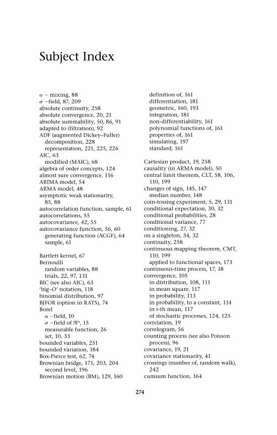
274
Subject Index
274
mixing, 88 field, 87, 209absolute continuity, 258absolute convergence, 20, 21absolute summability, 50, 86, 91adapted to (filtration), 92ADF (augmented Dickey–Fuller)
decomposition, 228representation, 221, 225, 226
AIC, 63modified (MAIC), 68
algebra of order concepts, 124almost sure convergence, 116ARIMA model, 54ARMA model, 48asymptotic weak stationarity,
85, 88autocorrelation function, sample, 61autocorrelations, 55autocovariance, 42, 55autocovariance function, 56, 60
generating function (ACGF), 64sample, 61
Bartlett kernel, 67Bernoulli
random variables, 88trials, 22, 97, 131
BIC (see also AIC), 63‘big–O’ notation, 118binomial distribution, 97BJFOR (option in RATS), 74Borel
field, 10 field of n, 15measurable function, 26set, 10, 33
bounded variables, 251bounded variation, 184Box-Pierce test, 62, 74Brownian bridge, 171, 203, 204
second level, 196Brownian motion (BM), 129, 160
definition of, 161differentiation, 181geometric, 160, 193integration, 181non-differentiability, 161polynomial functions of, 161properties of, 161simulating, 197standard, 161
Cartesian product, 19, 258causality (in ARMA model), 50central limit theorem, CLT, 58, 106,
110, 199changes of sign, 145, 147
median number, 148coin-tossing experiment, 5, 29, 131conditional expectation, 30, 32conditional probabilities, 28conditional variance, 77conditioning, 27, 32on a singleton, 34, 32continuity, 258continuous mapping theorem, CMT,
110, 199applied to functional spaces, 173
continuous-time process, 17, 18convergence, 105
in distribution, 108, 111in mean square, 117in probability, 113in probability, to a constant, 114in r-th mean, 117of stochastic processes, 124, 125
correlation, 19correlogram, 56counting process (see also Poisson
process), 96covariance, 19, 21covariance stationarity, 41crossings (number of, random walk),
242cumsum function, 164
Subject Index 275
data generation process, DGP, 66demeaning, 194, 224density function, 11, 12dependence, 27, 85derived probability measure, 11derived random variable, 5deterministic components, 213detrending, 194, 216, 224Dickey-Fuller
response function, 254tests, 205, 207, 218
diffusion process, 162discrete-time process, 17distribution function, 11domain, 259domain of attraction, 259
of the normal distribution, 259of a stable law, 176
drift, 218
efficient detrending, 229, 230, 240conditional distribution, 231unconditional distribution, 231
efficient markets, 156elementary events, 6ensemble averaging, 89ergodicity, 89
in the mean, 85, 91Eviews, 68exchange rate, 151expectation, 19
fair game, 93field (or algebra), 2, 6filtration, 92finite-dimensional distributions
(fidis), 19, 125F–measurablefractional differencing, 251frequency approach (to probability), 2function spaces
C[0, 1], 165, 167D[0, 1], 165, 167
functional, 172functional central limit theorem,
FCLT, 172
gambling, 130GARCH model, 93
generalised least squares, GLS, 232gold-silver price ratio, 153, 247
heteroscedasticity, 144
image, 259independence, 27, 36information criteria (IC), 63initial observation, 240, 250invariance, 218invariance principle, 172invertibility (in ARMA model), 50, 51Itô
calculus, 160, 182correction, 187formula, 187, 189exponential martingale, 190process, general, 191
Jensen’s inequality, 26joint distribution function, 32joint event, 30
kurtosis, 162
lag operator, 45lag polynomial, 46law of iterated expectations, 37Lebesgue measure, 16, 260Lebesgue–Stieltjes integral, 21limiting null distribution, 223,
229, 223linear dependence, tests, 61linear filter, 51‘little–o’ notation, 118Ljung-Box test, 62, 74local–to–unity, 229, 230long-run variance, 57, 80, 175, 246
estimation, 66parametric estimation, 68semi-parametric estimation, 66, 77
maintained regression, 206marginal distributions, 125Markov Chain, 130Markov process, 94, 130, 169martingale, 92, 93, 104, 130, 169
difference sequence (MDS), 49, 93, 144, 175, 179, 208
276 Subject Index
MATLAB, 79, 164mean reversion, 149, 243
unit root test, 241mean–reverting process, 214measure theory, 43measure zero, 34monotonic transformation,
159, 241moving average (MA), coefficients, 53multivariate normality, 36
near–integrated process, 229near–unit root, 205, 214, 215Newey-West kernel (weights), 67,
77, 247nonstochastic sequences, 106normal distribution, 6, 14
order of convergence, 118Ornstein-Uhlenbeck process, 191outliers, 251
partial sum process (psp), 31, 42, 93, 144
partial sums, 107path–wise variation, 169
quadratic, 169persistence, 52plim notation, 106Poisson distribution, 109
process, 95, 98polynomial regression, 120portmanteau test for linear
dependence, 62power (of test), 216, 236power function, 235power set, 3pre–image, 11, 260probability mass function
(pmf), 20probability measure, 2, 7probability space, 2pseudo–t statistic, 205
quadratic variation, 186quasi–differenced, QD, data,
231, 233
random variable, 1, 2, 5
continuous, 22, 31discrete, 12, 22, 27functions of, 23linear functions, 23nonlinear functions, 25
random vector, 15random walk, 129
approximation to BM, 177Gaussian inputs, 140, 149with drift, 140, 244no-change option, 140nonsymmetric, 139symmetric, 130, 141, 154symmetric binomial, 146, 157,
163, 244range, 20, 261RATS, 68Rayleigh distribution, 245real line, 261reflections, 148Reimann
definite, 183indefinite, 183integral, 21, 182, 186
Reimann–Stieltjesintegral, 183sum, 183
roots of the lag polynomial, 47
sample path, 19, 150sample paths (of BM), 162sample space, 2, 4
countably finite, 7countably infinite, 8uncountably infinite, 9, 21
scatter plot, 153seasonal pattern, 251second order stationarity, 41serial correlation, 220serial dependence, 58, 245short memory, 60, 72, 86sigma ratio, 234simulated distribution, 211–213slowly varying function, 261Slutsky’s theorem, 106, 114sojourn, 155speed of convergence, 126square summable, 91stationarity, 38

Subject Index 277
stochastic difference equation, 129, 160differential equation, 160process, 17
stochastic sequences, 106, 120stochastic sequences, Op(N)
notation, 120, 121stochastic sequences, op(n) notation,
120, 121stochastic unit root (STUR), 251Stratonovich integral, 185, 186strictly stationary process, 40strong law of large numbers, SLLN,
106, 117strong mixing, 86, 87, 174, 175strong white noise, 49sure convergence, 115
‘taking out what is known’, 37tally, 130temporal dependence, 85threshold autoregressive model
(TAR), 251time series, 45
breaks in, 250truncation rule, 67TSP, 68
unbounded variation, 169unconditional variance, 103uniform distribution, 13,
16, 179uniform joint distribution, 33unit root, 150
near cancellation, 250unit root test, 50, 165unit roots, multiple, 251US industrial production, 238US wheat production, 72
variance, 19of a sum of random variables, 25
weak dependence, 86, 176weak law of large numbers, WLLN,
106, 115weakly stationary process, 88white noise (WN), 31, 49