a prime mover - governor test model for large power
TRANSCRIPT

A PRIME MOVER - GOVERNOR TEST MODEL FOR LARGE POWER SYSTEMS
by
ROBERT GORDON SIDDALL
B.A.Sc., University of B r i t i s h Columbia, 1965
A THESIS SUBMITTED IN PARTIAL FULFILMENT OF THE
REQUIREMENTS FOR THE DEGREE OF
MASTER OF APPLIED SCIENCE
i n the Department of
E l e c t r i c a l Engineering
We accept t h i s thesis as conforming to the
required standard
Research Supervisor
Members of the Committee ,
Head of the Department
Members of the Department
of E l e c t r i c a l Engineering
THE UNIVERSITY OF BRITISH COLUMBIA
• January, 1968

In p r e s e n t i n g t h i s t h e s i s in p a r t i a l f u l f i l m e n t of the requirements f o r an
advanced degree at the U n i v e r s i t y of B r i t i s h Columbia, I agree that the
L i b r a r y s h a l l make i t f r e e l y a v a i l a b l e f o r reference and study. I f u r t h e r
agree that p e r m i s s i o n f o r e x t e n s i v e copying of t h i s t h e s i s f o r s c h o l a r l y
purposes may be granted by the Head of my Department or by h i s represen
t a t i v e s . I t i s understood that copying o r p u b l i c a t i o n of t h i s t h e s i s f o r
f i n a n c i a l gain s h a l l not be allowed without my w r i t t e n p e r m i s s i o n .
Department nf *A'I ttf C '^ih<^'-^/A^
The U n i v e r s i t y of B r i t i s h Columbia
Vancouver 8, Canada
Date ^JfltJ 3 f
ABSTRACT
This thesis i s concerned with the design, construction and t e s t i n g of a prime mover - governor model capable of simulating those components of a large power system. This unit i s to be used as part of a new power system test model. The model has been designed to simulate a prime mover - governor by c o n t r o l l i n g a laboratory-size dc motor through the f i e l d of a booster with allowance being made f o r s e t t i n g up the governor transfer functions, thus obtaining the desired torque and speed responses.
Since most methods of power system analysis neglect ce r t a i n system c h a r a c t e r i s t i c s and since tests on actual systems could be destructive, i t seems desirable to develop a complete power system test model capable of representing a r e a l power system f a i r l y accurately. When the system model i s completed, i t i s hoped that extensive transient s t a b i l i t y t ests can be carried out and r e a l system control techniques developed.
Chapter 2 of t h i s thesis outlines the design of the prime mover - governor model; Chapter.3 describes the r e a l i z a tion of the system; and Chapter 5 gives the model tests and r e s u l t s . The test methods and r e s u l t s of machine parameter measurements are included i n Chapter A.
i i

r
TABLE OE CONTENTS Page
ABSTRACT „ . ( i i ) TABLE OF CONTENTS ( i i i ) LIST OF ILLUSTRATIONS (v) LIST OF TABLES ( v i i ) LIST OF SYMBOLS ...» ( v i i i j ACKNOWLEDGEMENT £x) 1 . INTRODUCTION . > 0 0 8 1
1 . 1 Power System Studies • 1 1 . 2 Acceleration Equation of the Prime Mover and..
Governor •. • <..<>.... 3 1 . 3 Prime Mover - Governor Test Model 4
2 . ANALYSIS OF THE DC MACHINE EQUATIONS FOR THE PRIME MOVER - GOVERNOR TEST MODEL . . . „ ..„..„. 6 2 . 1 Torque-Speed Ch a r a c t e r i s t i c of a DC Motor i n
Series with a Booster . „ 6 2 . 2 Determination of the Booster F i e l d Voltage,
V f o 1 1
2 . 3 Relating the Units of the Torque Equations and R e a l i z a t i on of the Mechanical S t a r t i n g Time,
t t M f t M J o.. o... 13
2 . 4 The Load-Setting Resistor, R 14
3 . PROPOSED PRIME MOVER - GOVERNOR TEST MODEL 15
3 . 1 Speed Error C i r c u i t and F i l t e r . 15 3 . 2 Hydraulic Operator and Governor Transfer
Function Simulator . „ . . . 0 0 . . . . 18 3 . 3 DC Motor Torque Compensator .0. o.... 20 3 . 4 Booster F i e l d Time Constant Compensator 21 3 . 5 Booster F i e l d Current Amplifier .0 22 3 . 6 Power Supplies *. »...<> 25 3-.7 DC Motor, Booster, and Load-Setting Resistor . 28 3 . 8 The Complete System . 28
4. MEASUREMENT OF MACHINE PARAMETERS „ 30
'4 .1 Speed Voltage Coefficients . „ „ 30 4 . 2 I n e r t i a and No-Load Losses of the Tamper Set . 33
4 . 2 . 1 Loss Torque Expression ...„<,... <> 33 4 . 2 . 2 I n e r t i a of the Tamper Set . „. o.» ° 38
i i i
Page
4.. 3 R e s i s t a n c e and Inductance Measurements 41
5. TEST RESULTS „ . . . . . . . . . . 46
5.1 A n a l o g S t u d i e s of Governor R e p r e s e n t a t i o n and System Speed Responses . . . . . . . . . 46
5.2 A n a l o g Study of the Pr ime Mover - Governor Model . . . . . . . . . . 51
5.3 A n a l o g Study of the Model Response t o a J>0% l o a d R e j e c t i o n . „ . 55
5.4 R e a l Model T e s t s 5n
6. CONCLUSIONS . . 62
APPENDIX I The Machine A c c e l e r a t i o n E q u a t i o n 63
APPENDIX I I The Water A c c e l e r a t i o n E q u a t i o n . . . . . . . . . . 65
APPENDIX I I I The M e c h a n i c a l H y d r a u l i c Governor T r a n s f e r F u n c t i o n 68
REFERENCES 72
i v
LIST OF ILLUSTRATIONS Figure Page
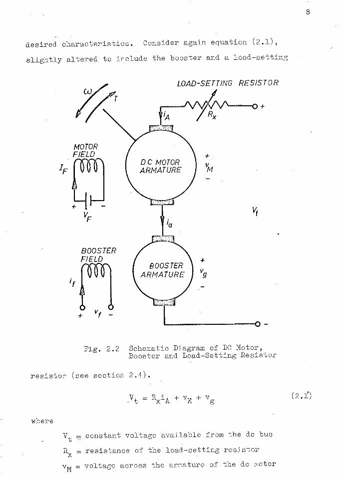
2.1 Separately Excited DC Motor 6 2.2 Schematic Diagram of DC Motor, Booster and Load-
Setting Resistor 8 2.1 Comparator C i r c u i t f o r Speed Error Signal 16 3.2 A Third Order Active F i l t e r 17 3.3 Hydraulic Operator R e a l i z a t i o n 19
3.4 DC Motor Torque Compensator 20
3.5 Lead Network f o r Booster F i e l d Time Constant Cancellation . „ „ 21
3.6 D i f f e r e n t i a t o r with Booster F i e l d Current Amplifier „ 23
3.7 Effect of Dead Zone and Zero Offset i n Current Amplifier . . o 24
3.8 Power Supply f o r Current Amplifier 27
3.9 Schematic Diagram of Complete System 29
4.1 C i r c u i t f o r Speed Voltage Coe f f i c i e n t Measurement 31
4.2 Determination of the Speed Voltage Coe f f i c i e n t f o r the Booster 32
4.3 Determination of the Coe f f i c i e n t L^, f o r the DC Motor o.o o . 32
4.4 C i r c u i t f o r the No-Load Torque Loss Test 34
4.5 Torque Versus F i e l d Current f o r Various Speeds .. 35
4.6 Plot of 'A' Versus 'co' and "Equation (4.12) 39
4.7 Plot of 'To' versus 'co' and Equation (4.13) 39
4.8 Retardation Curve f o r I n e r t i a Calculation 41
4.9 DC Motor Generator-Load Test 42
4.10 Booster Generator-Load Test 42
4.11 Inductance Measurement C i r c u i t 44
v
Figure Page •
4.12 Booster F i e l d Winding Current Response 44 5.1 Analog C i r c u i t f o r Equation (5.1) 47 5.2a Analog C i r c u i t f o r G-^p) ....................... 48 5.2b, Analog C i r c u i t f o r & 2(p) 48 5v2c Analog C i r c u i t f o r G^(p) 48 5.3 Speed Responses to a Step load Change 50 5.4 Analog Setup of the Prime Mover - Governor Model 53 5.5 Speed Response to a 30$ Load Rejection 56 5.6 Armature Current Response to the Load
Rejection 56 5.7 Booster F i e l d Voltage Response to the Load
Rejection .• 56 5.8 Steady State Speed Error Signal (Aw/2) 58 5.9 Speed Response of Actual System Compared to a
Simulation 60 5.10 Speed Response of Actual System Compared to a
Simulation 61 I I I - l Schematic Diagram of a Mechanical Hydraulic
Governor 69 I I I - 2 Plot of Actuator Piston V e l o c i t y versus P i l o t
Valve P o s i t i o n 68
v i
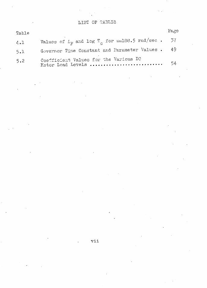
LIST OP TABLES Table Page 4.1 Values of i-p and l o g T q f o r eo=188.5 rad/sec . 37 5.1 Governor Time Constant and Parameter Values . 49 5.2 Coef f i c i e n t Values f o r the Various DC
Motor Load Levels 54
v i i

LIST OP SYMBOLS
A
a
DC Machines
dc motor armature current "booster " " dc motor f i e l d booster " " dc motor " voltage booster " " resistance and inductance of the dc motor armature
" " . " " " booster " • i t i ti tt f i e l d
f = ( l A+ L ) / ( R A + R + R - V ) ^ c motor-booster armature time constant
booster f i e l d time constant dc motor armature voltage booster " " dc bus voltage mechanical angular speed of the dc motor
11 " " 11 11 booster speed voltage c o e f f i c i e n t of the dc motor
II it I I I I n booster
v R A & L A
R & L a a R f & L f
r f - Lf / R
f
VM v g
V
w 00
coL
't
'AP g af
Prime - Mover Governor Model
R x
E oo +
J L
load-setting r e s i s t o r loss'torque of the model i n e r t i a of the complete Tamper set load torque on the dc motor
v x n
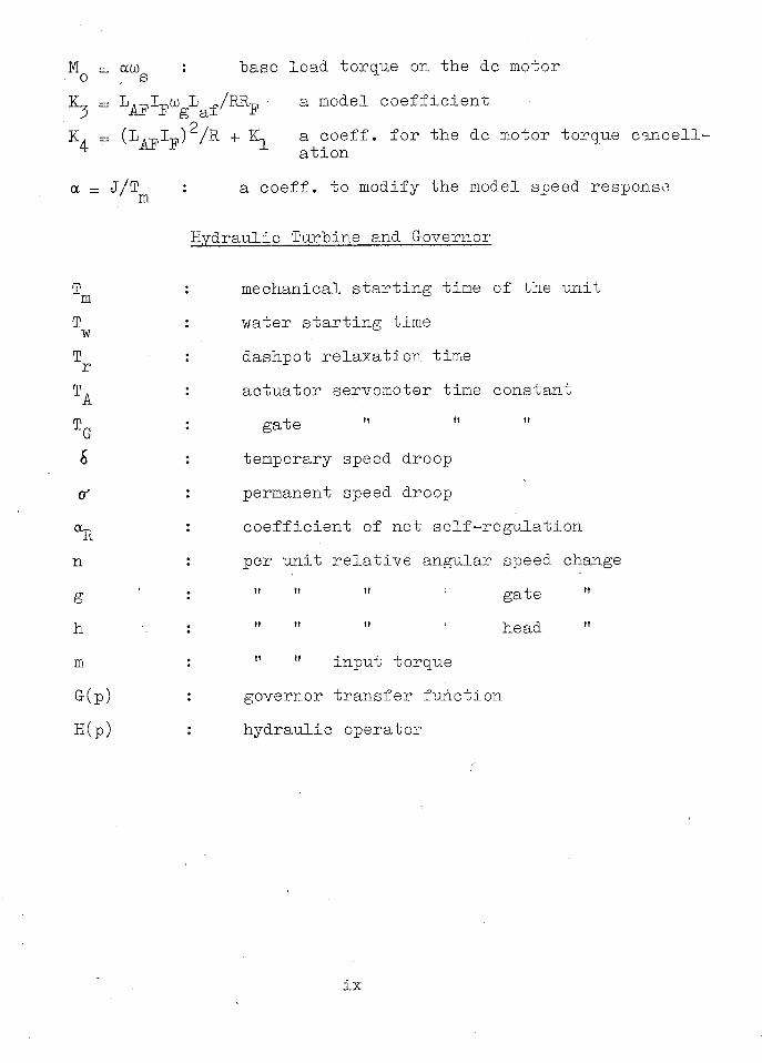
M = occo o s "base load torque on the dc motor
a model c o e f f i c i e n t K. = ( l . p l - n ) /R + K, a coeff. f o r the dc motor torque cancell-
4 M * L ation a = J/T m a coeff. to modify the model speed response
Hydraulic Turbine and Governor
m w T T A T 6
cf
R
n g h m G(p) H(p)
mechanical s t a r t i n g time of the unit water s t a r t i n g time dashpot r e l a x a t i o n time actuator servomotor time constant
gate " *' temporary speed droop permanent speed droop c o e f f i c i e n t of net s e l f - r e g u l a t i o n per unit r e l a t i v e angular speed change
i t I I G A T E -
I , I I I . M " " input torque
governor transfer function hydraulic operator
i x
ACKNOWLEDGEMENT
I wish to acknowledge my supervisor Dr. Yao-nan Yu and express my thanks f o r the guidance and encouragement given me during the course of my research.
I am indebted to Mr. Jamieson f o r reading the preliminary dr a f t and f o r h i s valuable comments.
I also wish to thank Mr. G. Dawson and Mr. A. Mackenzie i n p a r t i c u l a r and the many others who were always w i l l i n g to be of assistance when I needed i t .
Acknowledgement i s given to the National Research Council f o r . f i n a n c i a l support of the research.
x
1
INTRODUCTION
1.1 Power System- Studies
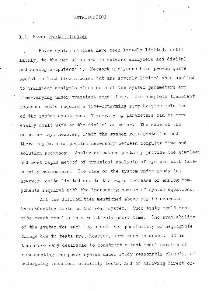
Pover system studies have been l a r g e l y l i m i t e d , u n t i l l a t e l y , to the use of ac and dc network analysers and d i g i t a l and analog c o m p u t e r s . Network analysers have proven quite . useful i n load flow studies but are severly l i m i t e d when applied to'transient analysis since some of the system parameters are time-varying under transient conditions. The complete transient response would require a time-consuming step-by-step s o l u t i o n of the system equations. Time-varying parameters can be more e a s i l y dealt with on the d i g i t a l computer. The si z e of the computer may, however, l i m i t the system representation and there may be a compromise necessary between computer time and solution accuracy. Analog computers probably provide the simplest and most rapid method of transient analysis of systems with time-varying parameters. The size of the system under study i s , however, quite l i m i t e d due to the rapid increase of analog components required with the increasing number of system equations.
A l l the d i f f i c u l t i e s mentioned above may be overcome by conducting tests on the r e a l system. Such tests could provide exact r e s u l t s i n a r e l a t i v e l y short time. The a v a i l a b i l i t y of the system f o r such tests and the _ p o s s i b i l i t y of n e g l i g i b l e damage due to tests are, however, very much i n doubt. I t i s therefore very desirable to construct a test model capable of representing the power system under study reasonably c l o s e l y , of undergoing transient s t a b i l i t y t e s t s , and of allowing d i r e c t on-
2
l i n e instrumentation and control . 'Micromachine' and 'micronetwork' models have been
(2) (3) developed and designed by Robert i n France, Venikov i n Russia, and Ad k i n s ^ ^ i n Great B i i t a i n to include such e f f e c t s as the damping and saturation as i n r e a l machines and the e x c i t a t i o n and governor controls usually neglected i n system studies. They a l l used small synchronous machines to represent the large generators and small dc motors to represent the prime movers. Some type of negative resistance c i r c u i t was used to obtain the desired f i e l d time constant while desired machine i n e r t i a was obtained by means of an adjustable flywheel. Based on a c r i t e r i a of s i m i l a r i t y of e l e c t r i c a l and mechanical c h a r a c t e r i s t i c s , a power system composed of large machines can thus be represented by much smaller machines.
.One of the projects of the power group at U.B.C. i s to develop a power system test model along s i m i l a r l i n e s to those of the micromachines. This thesis i s pr i m a r i l y concerned with the development of a universal test model to simulate turbine and governing systems of various types and sizes using small laboratory dc machines. A sp e c i a l analog computer i s designed to allow considerable freedom i n s e t t i n g of desired time constants by simple potentiometer adjustments. Control signals are also r e a l i z e d on the computer to cancel undesired dc machine c h a r a c t e r i s t i c s . The necessity of an adjustable flywheel i s eliminated by the use, of a gain potentiometer on the computer. The model thus constructed allows the simulation of most turbine and governing systems.

3
The prime mover-governor model, i n conjunction with a *
s o l i d state e x c i t e r and voltage regulator already completed and a generator and transmission system being developed, w i l l provide a complete test model for a large power system.
1.2 Acceleration Equation of the Prime Mover and Governor
The mechanical c h a r a c t e r i s t i c s of the power system, the prime mover with governor, are represented by the acceleration equation which r e l a t e s the generator-prime mover acceleration to applied torques (see Appendix I ) . Hovey and Bateman^^, i n t h e i r paper on speed regulation t e s t s , give the per unit acceleration equation as
T pn = m - oun - Am ( l . l ) m r .hi
Eor the l i s t of symbols see page v i i i . The per unit input torque, 'm', depends on the governing
of the unit under study. In the case of a steam plant, Concordia and K i r c h m a y e r , i n t h e i r paper on t i e - l i n e and f r e quency c o n t r o l , give the speed governor response as a function of only one time constant, T^, where T^ i s the t o t a l time l a g associated with the equivalent governor and steam turbine. The input torque i s
m = T l + T l P) (1 + T l P) ^ C 1' 2)
In the case of a hydraulic plant, the input torque equation i s more complicated due to the effect of water column i n e r t i a . Based cn papers by H o v e y a n d discussions of related papers by Paynter , the equation r e l a t i n g input torque and speed
4
may "be w r i t t e n as
m = : (-n) ( T
AT
rp
2
+ ( TA + ( r + i ) T
r) p + f ) (1 + T
&p) (1 + .5T
wp)
(1.3)
Neglecting some of the governor parameters, equation ( l . 3 ) may
be approximated by equation (1.4) without too great an error
i n t r ansient response i n some cases,
(1 + T„p) (1 - T wp m = r - ^ f_n) • (1.4)
( STrp) (1 + .5T
wp!
Appendices II and I I I , based on works by H o v e y ^ and B i c h ^ ^ ,
give the deri v a t i o n s of the water a c c e l e r a t i o n equation and the
mechanical governor t r a n s f e r function from which equation (1 . 3 )
i s obtained.
1.3 Prime Mover - Governor Test Model
Since s t a b i l i t y studies w i l l be c a r r i e d out mainly f o r
h y d r o - e l e c t r i c systems with mechanical governing,- the model i s
designed to duplicate the per uni t torque-speed c h a r a c t e r i s t i c s
of the hydraulic t u r b i n e . These c h a r a c t e r i s t i c s are obtained ,
• from equation ( l . l ) a f t e r s u b s t i t u t i o n of equation (1 . 3 ) f o r the
input torque
(1+T p) 1 (1-T p) T pn = 5 • (-n) - cc
Rn-Am
m
( TAT
rp
2
+ ( TA + <ST
r)
P) (1+T
& P) (l+.5T
wp)
(1.5)
5
The modelling of a steam plant should quite e a s i l y follow since i t s input torque-speed r e l a t i o n s h i p , comparing equation (1.2)
with ( 1 . 3 ) , i s much simpler than that of the hydraulic p l t n t . Consideration has been given to other types of prime
movers to simulate the hydraulic turbine: a scaled down hydraulic model, a small synchronous motor, a small induction motor, or a small dc-motor. The scaled hyraulic model i s rejected immediat e l y a f t e r consideration of the i m p r a c t i c a l i t i e s involved i n construct/ion. Although the synchronous and induction motors off e r a more p r a c t i c a l s o l u t i o n , overly complex controls would be required i n order to obtain the desired torque-speed characteri s t i c . E l i m i n a t i n g the above mentioned three leaves only the dc motor, as used with the micromachine s y s t e m s 3 ) (4) ^ ^ 0
represent the hydraulic turbine. Chapters 2 ,3 , and 4 of t h i s thesis show the development
and construction of the test model using a dc motor to simulate the hydraulic turbine and governing system and Chapter 5 gives the test r e s u l t s of the model.

6
2 / ANALYSIS OP THE DC MACHINE EQUATIONS FOR THE
PRIME MOVER - GOVERNOR TEST MODEL
2.1 Torque-Speed C h a r a c t e r i s t i c of a DC Motor i n Series with
a Booster
The reason f o r choosing a dc motor to simulate the
hydraulic turbine i s that adequate speed and torque c o n t r o l
can be r e a l i z e d f a i r l y simply over a wide range. There are
three main methods of c o n t r o l l i n g the speed of the dc motor:
by varying armature r e s i s t a n c e , by varying the e x c i t a t i o n ,
and by varying the armature terminal v o l t a g e . Consider
equation (2.1) f o r the separately excited dc motor of Figure 2.1.
F i g . 2-1 Separately Excited DC Motor
Vt = R i
A + coL^ip (2.1)

V t - R i A or co = - r — : •
i JAP 1F where
co = the mechanical angular spewed of the machine wL -p = the speed voltage c o e f f i c i e n t
= a c o e f f i c i e n t defined from the speed voltage coeff. and the mechanical angular speed
R = armature resistance i ^ = armature current
= e x c i t a t i o n current = armature terminal voltage
I t can be seen that the speed may be c o n t r o l l e d by varying Y^,
R, or i-p. To achieve speed control by varying resistance i n the armature c i r c u i t requires mechanical devices such as a manually operated rheostat which may r e s u l t i n discrete rather than continuous c o n t r o l . Although speed control of the motor can be achieved by varying the f i e l d current, the control required to obtain the desired torque-speed c h a r a c t e r i s t i c would be very complicated. This leaves the control of voltage across the armature of the dc motor as the only means by which to obtain the desired torque-speed c h a r a c t e r i s t i c of the hydraulic prime mover.
Armature voltage control i s r e a l i z e d by connecting a booster i n series with the armature- of the dc motor. Given a constant l i n e voltage, the voltage across the armature of the dc motor Is varied by c o n t r o l l i n g the output voltage of the booster which i s achieved by adjusting i t s f i e l d voltage.
The system equations f o r Figure 2.2 are examined i n order to determine the exact form of control necessary to r e a l i z e the
8
desired c h a r a c t e r i s t i c s . Consider again equation ( 2 . l ) , s l i g h t l y altered to include the booster and a loa d - s e t t i n g
where tz constant voltage available from the dc bus
R = resistance of the load-setting r e s i s t o r v M = voltage across the armature of the dc motor
9
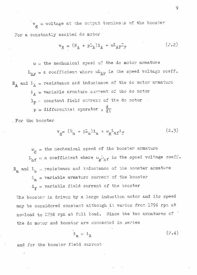
Vg = voltage at the output terminals of the booster
For a constantly excited dc motor
VM = ( R A + p L A ) ; L A + ^ A F ^ ( " ' 2 ;
co = the mechanical speed of the d-c motor armature
IjAF = a c o e f f i c i e n t where coL^p i s the speed voltage coeff,
B. and = resistance and inductance of the dc motor armature
i A = v a r i a b l e armature current of the dc motor
I-p = constant f i e l d current of the dc motor
p = d i f f e r e n t i a l operator ,
. For the booster
vg= ( R a + P L a } i a + V a ^ f ( 2 ^
co = the mechanical speed of the booster armature
L „ = a c o e f f i c i e n t where co L „ i s the speed voltage coeff. s i g a i
R and L = resistance and inductance of the booster armature a a i = v a r i a b l e armature current of the booster a i ^ , = v a r i a b l e f i e l d current of the booster
The booster i s driven by a large induction motor and i t s speed
may be considered constant although i t v a r i e s from 1796 rpm at
no-load to 1794 rpm at f u l l load. Since the two armatures of
the dc motor and booster are connected i n s e r i e s
i a = i A (2.4)
and f o r the booster f i e l d current

10
v f v f 1
i f = R^ + L f p = R^T ( i + r f P)" ( 2 , 5 )
R„ and = r e s i s t a n c e and inductance of the booster f i e l d w i nding
L f = — = the booster f i e l d time constant
= the c o n t r o l v o l t a g e a p p l i e d to the booster f i e l d
S u b s t i t u t i n g equations ( 2 . 2 ) through ( 2 . 5 ) i n t o equation (2.l')
and s o l v i n g f o r i ^ y i e l d s
1 w "^af = R ( I + r P ) — ( v t - ^ A P ^ - R f ( i V t * f P ) V ( 2 ' 6 ;
where R = R + R . + R . Q, i i X
I t i s found from t e s t s t h a t the time constant of the armature
c i r c u i t , T ,
where T , T
L A :+ L a \ * RA + R x
i s r e l a t i v e l y s m a l l (see s e c t i o n 4.3) and may be negl e c t e d as
compared w i t h other time constants of the r e q u i r e d t r a n s f e r
f u n c t i o n s , thus
-, w L _p ^ = R ^ V t - ^ A F 1 ? - R f ( l fr f P) V f } ( 2 ' 6 < )
The torque equation of the dc motor i s
J + K l w + K 2 = L A P I F I A ~ L ( 2 . 7 )
11
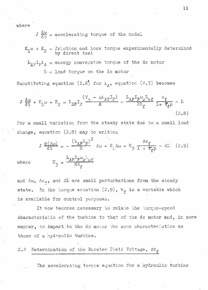
where J —^ = accelerating torque of the model
K,w + Kp = f r i c t i o n and loss torque experimentally determined by d i r e c t test
L^-plpi^ = energy conversion torque of the dc motor L = load torque on the dc motor
Substit u t i n g equation (2.6f) f o r i ^ , equation (2.7) becomes
j d a _ M + K j (v t - C O L A F I f ) l A F I F c o g l a f v f
dt K 1 W + K
2 = R R R F 1+ r fp " L
(2.8) For a small v a r i a t i o n from the steady state due to a small load change, equation (2.8) may be written
T d(Aco) ^ A F 1 ^ A 77- * v A v f A T , 0 n N
J d t = R — A w - K i A w - K 3 r r - ^ - A L ( 2 ' 9 )
where K, = * a I
3 R K ^
and Aco, Av^, and AL are small perturbations from the steady state. In the torque equation ( 2 . 9 ) , i s a variable which i s available f o r control purposes.
I t now becomes necessary to relate the torque-speed c h a r a c t e r i s t i c of the turbine to that of the dc motor and, i n some manner, to impart'.to the dc motor the same c h a r a c t e r i s t i c s as those of a hydraulic turbine.
2.2 Determination of the Booster F i e l d Voltage, Av^
The accelerating torque equation f o r a hydraulic turbine

under small load v a r i a t i o n s may be wr i t t e n i n per unit quantities (see also Appendix I) as
Tm IT = & ( p ) H ( p ) ( - n ) -«Rn - Am (2.10;
I •rr = accelerating torque which i s zero under m steady state conditions
G(p)H(p)(-n) = input torque change to the hydraulic turbine due to the speed change
oc n = damping torque on the hydraulic turbine Am = torque change due to generator load
v a r i a t i o n s
The governor transfer function G-(p) has a number of forms (see Appendix I I I ) the simplest of which being
1 + T p G(p) = — (2.11a)
<5T p and the hydraulic operator H(p) has the form (see Appendix II)
1 - T p H(p ) = ^ (2.11b)
1 + 0.5T P
w
In order to r e a l i z e the torque-speed c h a r a c t e r i s t i c of a hydraulic turbine with a mechanical governor on a dc motor with series booster, the two sets of values, I , Am, and n i n
' ' m' ' equation (2.10) and J, A L , and AGO i n . equation ( 2 . 9 ) , are treated analogously. A gain factor a i s introduced to take care of di f f e r e n t units of equation (2.9), i n M K S , and equation (2.10)
i n per u n i t . Comparison of these two equations y i e l d s - K4Aco - 1 +
?r ^ p Av f = cc(G(p)H(p) + a R) (-Aa>) (2.12)

13
where K^ = + K.
a = the gain factor to be determined shortly-
Solving f o r Av^ gives the required booster f i e l d voltage
1 + t f p Av f = |a(G(p)H(p)+a R) - (Aw) ( 2 . 1 3 )
2 . 3 Relating the Units of the Torque Equations and Re a l i z a t i o n of the Mechanical S t a r t i n g Time, T m
Substitu t i n g equation ( 2 . 1 3 ) into equation ( 2 . 9 ) r e s u l t s
i n J = a(G(p)H(p)+a R) (-Aco) - AL ( 2 . 1 4 )
which i s s i m i l a r to equation ( 2 . 1 0 . ) . Since the dc motor torque equation ( 2 . 9 ) and hence ( 2 . 1 4 ) are wri t t e n i n MKS u n i t s , and since (G-(p)H(p) + oc ) i s dimensionless, ocAco must have the units of torque or newton-meters and thus 'a' must have the units , 2 kg-m sec
Equations ( 2 . 1 4 ) and ( 2 . 1 0 ) are. w r i t t e n i n d i f f e r e n t u n i t s , MKS and per unit respectively. To convert equation ( 2 . 1 4 ) to per un i t i t i s necessary to divide through by the rated speed co and a thus obtaining s &
£ ^ = G ( p ) H ( p ) ( - n ) - ^ " - R n ( 2 . 1 5 ) s
where n = ~ per unit .angular speed, s
Comparison of the turbine equation ( 2 . 1 0 ) and the dc motor equation ( 2 . 1 5 ) shows that equality of per unit torque-speed

14
respons-e may be obtained by s e t t i n g
— _ T or a = i - ( 2 . 1 6 ) a m T m
Since AL/aw corresponds to the per unit torque change and s AL i s the torque change on the dc motor, the base torque of the
motor must equal
M N t aw . (.2 .17)
M q = base load torque on the dc motor
The base load torque w i l l vary with the actual unit being simulated since, while w i s a constant, a varies with T whose ' s ' m value' depends on the system being examined.
2 . 4 The Load-Setting Resistor, R •
The s o l u t i o n f o r the Av f s i g n a l i n equation ( 2 . 1 3 ) i s derived from the speed v a r i a t i o n , Aw, due to a load change from the steady state. In order to maintain a base load on the synchronous machine at synchronous speed p r i o r to a load r e j e c t i o n t e s t , the energy conversion torque of a constantly excited dc motor requires a cer t a i n armature current. This currentmay be obtained by adjusting either the load-setting r e s i s t o r i n the armature c i r c u i t or the booster armature voltage or both. Since the booster armature voltage i s designed to respond to load va r i a t i o n s only, the armature current f o r steady state load i s set by the load-setting r e s i s t o r .

15
3. . PROPOSED PRIME MOVER - GOVERNOR TEST MODEL
The proposed simulation of the hydraulic turbine and governor by a dc motor with controls i s made up of s i x parts; the speed error c i r c u i t and f i l t e r , the hydraulic operator and governor transfer function simulator, the dc motor torque compensator, the booster f i e l d time constant compensator, the f i e l d current a m p l i f i e r , and the dc motor and booster including the l oad-setting r e s i s t o r and dc tachometer, which are described i n the following sections. The complete system diagram i s shown i n Figure 3.9.
3.1 ' Speed Error C i r c u i t and F i l t e r
The booster f i e l d voltage Av^, equation (2.13), f o r the torque-speed control of the dc motor i s a function of the speed deviation
1 + T-FP Av f = —g~-(a(G(p)H(p)+a R)Aco - K^Aw) (2.13)
Since Av^ i s r e a l i z e d on a specialized analog computer, Aw,is required as a voltage s i g n a l .
A-voltage si g n a l proportional to the speed of the generator-turbine model i s obtained from a small SERVO-TEK dc • tachometer mounted through gears to the shaft of the synchronous generator. The tachometer has a voltage output of 20„8 v o l t s per thousand rpm and, hence, 37.44 v o l t s at the synchronous speed, 1800 rpm or 188.5 rad/sec. The gearing of the tachometer to the

16
genera'tor shaft increases the speed of the tachometer by a factor of 2 . 5 . I t s voltage output i s thus increased to 9 3 . 5
v o l t s for the model running at synchronous speed. The output of the tachometer now requires a m u l t i p l i c a t i o n f a c t o r of 2.012, (188.5 / 9 3 . 5 ), i n order that the speed voltage l e v e l be read d i r e c t l y i n rad/sec ( l v o l t = 1 rad/sec). The reason f o r mechanically increasing the tachometer speed i s to reduce the m u l t i p l i c a t i o n f a c t o r and the accompanying gain i n noise l e v e l of the operational a m p l i f i e r s .
By increasing the tachometer s i g n a l by a. constant factor (k-^ - 1.006) and applying i t to 'a comparator, which i s an operational a m p l i f i e r summer, along with a reference s i g n a l , one hal f the speed error s i g n a l i s obtained. The factor of one ha l f i s made up l a t e r i n the c i r c u i t .
TA CH0METER-93-5V / Q \ ' 9 4 ' 2 S V s J i OUTPUT --^ U \ K 1 J
+94-25 V= + (£s
(OS.) REFERENCE Q 1 _ SPEED SIGNAL 1-006
F i g . 3.1 Comparator C i r c u i t for Speed Error Signal
The signal-to-noise r a t i o of the tachometer i s approximately 1:0.1. Because of the presence of a d i f f e r e n t i a t o r i n a succeeding part of the c i r c u i t , i t was necessary to reduce the signal-to-noise r a t i o to approximately 1:0.0002 by passing the
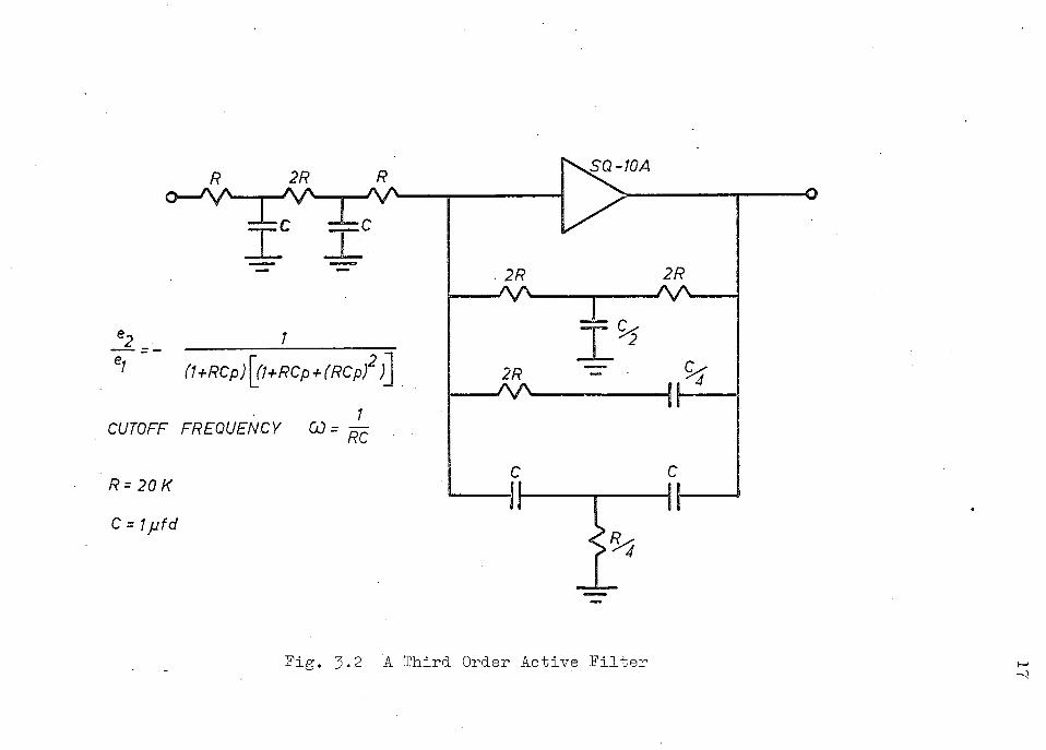
R o — ' N A
2R A A
X CV ~ X
•I ^ » I I l . —
A A
(l+RCp) (1+RCp + (RCp)2)_
CUTOFF FREQUENCY OJ = ^
R = 20K
C=1pfd
• 2R A A
2R A A -
c
tt
wSQ-70>4
2 A
P i g . 3.2 A Third Order Active ..Filter

18
( l G )
0.5 AOJ s i g n a l through an active t h i r d order f i l t e r as shown i n Figure 3.2. 3.2 Hydraulic Operator and G-overnor Transfer Function -Simulator
By combining equations (2.11a) and (2.11b), the transfer functions of the mechanical hydraulic governor and the hydraulic operator are written
(1 + T p ) ( l - T p) G(p)H(p) = 2 (j.!)
(8 T rp) (1 + .5T wp)
The actual values of the time constants and parameters depend upon the system being examined. A s p e c i a l i z e d analog computer has been b u i l t to r e a l i z e the required booster f i e l d voltage. The above transfer functions, equation (3.1), required f o r the f i e l d voltage s i g n a l , may be set up on t h i s computer either
(12) by a lead-lag network method or by a d i v i s i o n a l method '. Since the d i v i s i o n a l method provides a simple means of parameter adjustment by s e t t i n g potentiometers, the method i s adopted. For example, f o r the hydraulic operator, l e t t i n g the input sig n a l be ' e^' and the output s i g n a l be 'e^' there r e s u l t s
( l - T p) = 2 ( ) ( 3 > 2 a )
2 (1 + -5Twp) 1
which may be rewritten as i
^1 ^1 ^2 e2 = 0.5T p 075 ~ 0.5T p (3.2b) w w
from which the output i s obtained using summing and integrat i n g components. Figure 3«3 shows the analog c i r c u i t used to

POTENTIOMETER
F i g . 3.3 H y d r a u l i c Operator R e a l i z a t i o n
obtain the desired hydraulic operator with the parameter T w
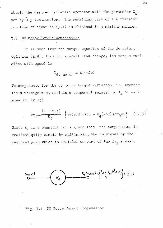
set by a potentiometer. The remaining part of the transfer function of equation ( 3 . 1 ) i s obtained i n a s i m i l a r manner. 3 . 3 DO Motor Torque Compensator
I t i s seen from the torque equation of the dc motor, equation ( 2 . 9 ) , that f o r a small load change, the torque v a r i a t i o n with speed i s
T , , = K . (-Aco) dc motor 4
To compensate f o r the dc motor torque v a r i a t i o n , the booster f i e l d voltage must contain a component related to Aco as i n .equation ( 2 . 1 3 )
(1 + ?pp) r / • A v f = g— - — < ccG(p)H(p)Aco + K^-Aco) +aaRAcoV ( 2 . 1 3 .
3
Since Is a constant for a given load, the compensator i s r e a l i z e d quite simply by mult i p l y i n g the Aco sig n a l by the required gain which i s included as part of the Av f s i g n a l .
O 4 K4 J ^ - O I R J
P i g . 3 . 4 DC Motor Torque Compensator

3.4 Booster F i e l d Time Constant Compensator
2 1
According to equation (2.13) a d i f f e r e n t i a t o r c i r c u i t i s necessary to obtain the required booster f i e l d voltage s i g n a l s o that equation (2.12) i s s a t i s f i e d . The d i f f e r e n t i a t o r c i r c u i t cancels the e f f e c t of the booster f i e l d time constant as i n cluded i n equation (2.12)
-K.Aco - z 2xr-• Av_p = ocG(p)H(p) (-Aco)-ocapAio (2.12) 4 1 + Cj?p I JA
The d i f f e r e n t i a t o r , as shown i n Figure 3.5? i s r e a l i z e d using a lead network. Since the time constant i s f i x e d , adjustment of the network i s not required.
F i g . 3.5 lead Network f o r Booster F i e l d Time Constant Cancellation
A current balance at node 'g' gives

V 1 + p ° d V
R d ( i + P C V V (3.3)
where C^R^ - f = 0 . 5 .
The capacitor C. i s included (11) to s t a b i l i z e the d i f f e r e n t i a t o r c i r c u i t and provides a f i l t e r i n g e f f ect for high frequencies.
approximately by a factor of 10.
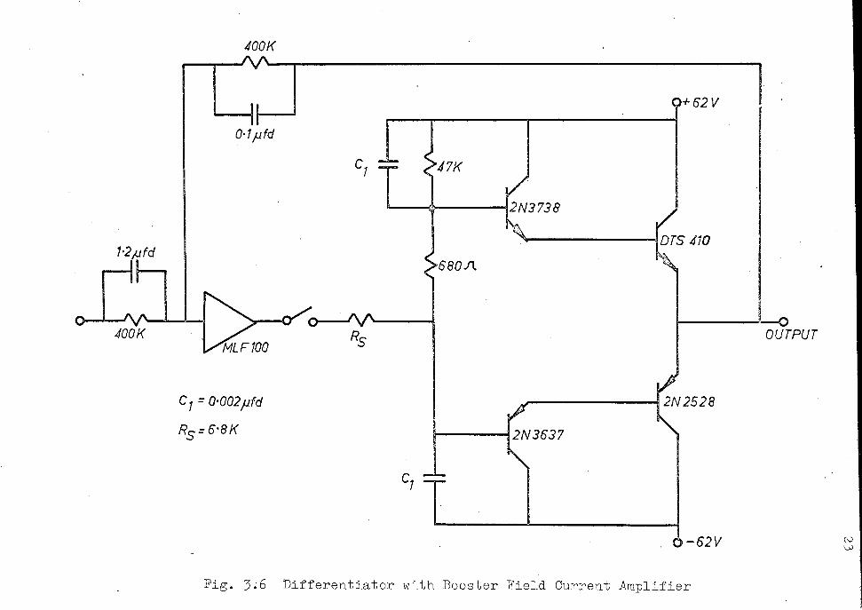
3.5 Booster F i e l d Current Amplifier
The output of the d i f f e r e n t i a t o r provides the control s i g n a l , v_g., for the booster. Since the maximum output of the operational a m p l i f i e r of the d i f f e r e n t i a t o r i s 100 v o l t s and 10
milliamps while the booster f i e l d i s rated at 1.25 amps at 64.5
v o l t s , a current a m p l i f i e r Is necessary to meet the current requirements of the f i e l d .
The current a m p l i f i e r , as shown i n Figure 3.6, Is made up of two symmetrical c i r c u i t s with one side amplifying the p o s i t i v e sig n a l s , the other side, the negative. Each side consists of a complementary common-collector pair of tr a n s i s t o r s i n a Darlington configuration. Since the current gain f o r a single
fl^) t r a n s i s t o r common-collector ampl i f i e r i s
The magnitude of R^, however, i s maae much smaller, than C R
A ± « (p + 1)
where p i s the common-emitter short c i r c u i t current gain, the Darlington configuration r e s u l t s i n a current gain of
A. a (p + 1)(p + 1)
Although the voltage gain i s e s s e n t i a l l y unity, there
400K A A -
1-2/jfd
H h
O — « — f \ / ^
400K
0-1 pfd
C\ =b >47K
I2N3738
»680Sl
Cj= 0-002pfd
RS = 6'8K 2N3637
Q+62V
IDTS 4W
OUTPUT
2 N 2528
•62V
F i g . 3 . 6 D i f f e r e n t i a t o r with Booster F i e l d Current Amplifier

F i g . 3.7 E f f e c t of Dead Zone and Zero O f f s e t i n C u r r e n t A m p l i f i e r

t
2 5
e x i s t s a small voltage drop across the base-emitter junctions which i s approximately independent of input voltage. These voltage drops create a dead zone of approximately 2 v o l t s at zero input. There also e x i s t s an output voltage offset of approx-1- • imately -0.3 v o l t s f o r zero input due to the leakage current of the PNP t r a n s i s t o r s . By placing the current a m p l i f i e r inside the feedback loop of the operational a m p l i f i e r and'by turning the NPN t r a n s i s t o r s s l i g h t l y on, the zero voltage offset i s corrected to approximately +0.1 v o l t s and the d i s c o n t i n u i t y at the zero crossing Is reduced to zero. The test r e s u l t s are shown In Figure 3.7.
The current a m p l i f i e r i s protected to some extent by the current l i m i t i n g c i r c u i t and by fuses i n the power supplies.
3.6 Power Supplies
Three power supplies are required f o r operation of the prime mover - governor model, two f o r the operational amplifiers and reference voltage signals, and one for the booster f i e l d a m p l i f i e r , i n addition to the dc motor-booster power supplies.
Power supply 1 provides a well-regulated, low noise + 120 v dc supply f o r the 100 v operational amplifiers and also provides + 120 v dc as required for the speed s i g n a l reference. Power supply 2 provides a well-regulated low noise + 15 v dc supply for the 10 v operational a m p l i f i e r s . Both power supplies were obtained commercially.
Power supply -3 i s designed and constructed to provide a + 62 v dc supply for the booster f i e l d current a m p l i f i e r . The
26
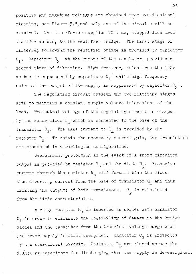
p o s i t i v e and negative voltages are obtained from two i d e n t i c a l c i r c u i t s , see Figure 3.8, and only one of the c i r c u i t s w i l l be examined. The transformer supplies 70 v ac, stepped down from the 120v ac bus, to the r e c t i f i e r bridge. The f i r s t stage of f i l t e r i n g f o llowing the r e c t i f i e r bridge i s provided by capacitor C- . Capacitor 0^, at the output of the regulator, provides a second stage of f i l t e r i n g . High frequency noise from the 120v ac bus i s suppressed by capacitors C- while high frequency noise at the output of the supply i s suppressed by capacitor C^'.
The reg u l a t i n g c i r c u i t between the two f i l t e r i n g stages acts to maintain a constant supply voltage independent of the load. The output voltage of the regulating c i r c u i t i s clamped by the zener diode D which i s connected to the base of the t r a n s i s t o r Q . The base current to i s provided by the r e s i s t o r R . To obtain the necessary current gain, two t r a n s i s t o r s are connected i n a Darlington configuration.
Overcurrent protection i n the event of a short c i r c u i t e d output i s provided by r e s i s t o r R^and the diode D . Excessive current through the r e s i s t o r R w i l l forward bias the diode & p thus d i v e r t i n g current from the base of t r a n s i s t o r and thus l i m i t i n g the outputs of both t r a n s i s t o r s . R^ i s calculated from the diode c h a r a c t e r i s t i c .
A surge r e s i s t o r R i s inserted i n series with capacitor C- i n order to eliminate the p o s s i b i l i t y of damage to the bridge diodes and the capacitor from the transient voltage surge when the power supply i s f i r s t energized. Capacitor i s protected by the overcurrent c i r c u i t . Resistors R-g are placed across the f i l t e r i n g capacitors for discharging when the supply i s de-energized.
F i g . 3.8 Power Supply f o r Current Amplifier to
28
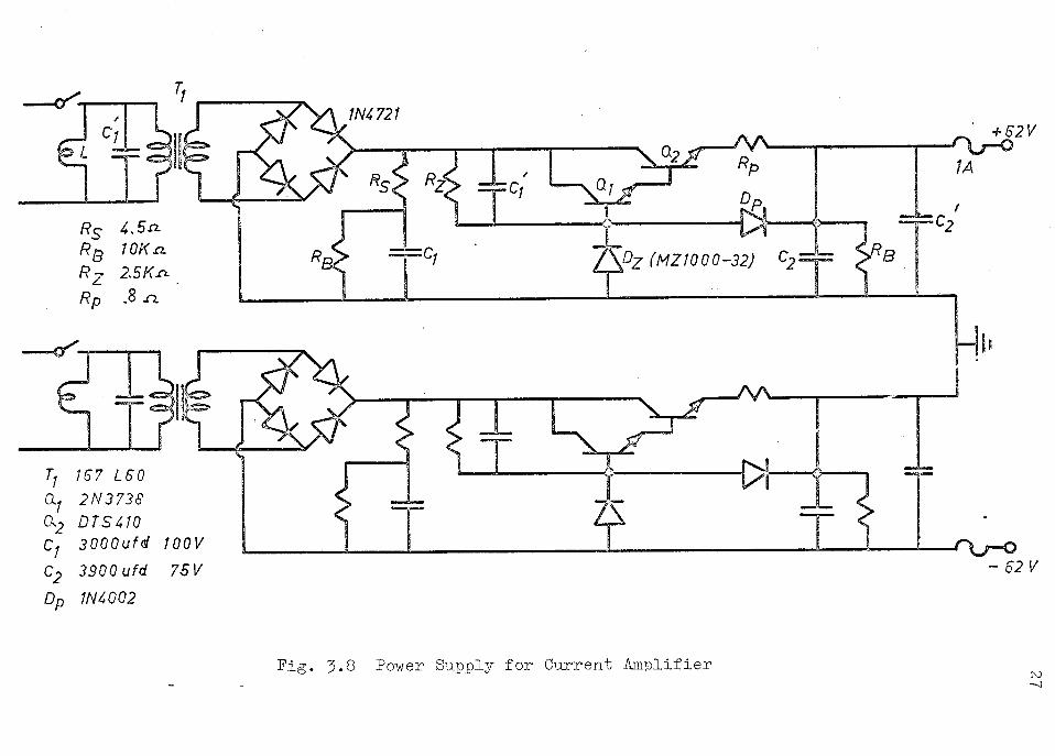
3.7 DC Motor, Booster, and Load-Setting Resistor
A schematic diagram of the dc motor, booster, and load-s e t t i n g r e s i s t o r i s shown i n Figure 2.2.
The dc motor f i e l d i s separately excited with a constant current of 0.5 amps and the armature i s connected i n series with the booster and the load-setting r e s i s t o r . The source supply i s 230v dc. The dc motor i s part of a Tamper Set which consists of an induction machine, a dc machine, and a synchronous machine mounted on the same stand with flange couplings allowing them to be connected together. The i n e r t i a of the dc motor-synchronous generator set i s increased by including the rotor of the induction machine through coupling.
The booster i s driven by an induction motor and i s separately excited by the booster f i e l d voltage s i g n a l v^ which provides a variable e x c i t a t i o n . The speed of the induction motor varies only from 1796 rpm at no load to 1794 rpm at f u l l load and i s therefore deemed constant.
The load-setting r e s i s t o r R has been described i n section 2.4.
3.8 The Complete System
Figure 3.9 i s a schematic diagram, of the complete system. The section enclosed by dotted l i n e s i s that part of the equipment which i s rack mounted.

TACHOMETER
.LOAD - SETTING RESISTOR
DC BUS VOLTAGE (Vt)
SPECIAL ANALOG COMPUTER
SPEED ERROR FILTER
GOVERNOR TRANSFER FUNCTIONS
BOOSTER FIELD TIME CONSTANT COMPENSATOR AND CURRENT AMPLIFIER
ro F i g . 3.9 - S c h e m a t i c D i a g r a m o f C o m p l e t e S y s t e m
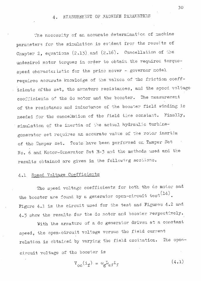
4. MEASUREMENT OP MACHINE PARAMETERS
30
The necessity of an accurate determination of machine
parameters f o r the simulation i s evident from the r e s u l t s of
Chapter 2, equations (2.13). and (2.16). Cancellation of the
undesired motor torques i n order to obtain the required torque-
speed c h a r a c t e i i s t i c f o r the prime mover - governor model
requires accurate knowledge of the values of the f r i c t i o n coeff
i c i e n t s ofthe s e t , the armature r e s i s t a n c e s , and the speed voltage
c o e f f i c i e n t s of the dc motor and the booster. The measurement
of the r e s i s t a n c e and inductance of the booster f i e l d winding i s
needed f o r the cancellation of the f i e l d time constant. F i n a l l y ,
simulation of the i n e r t i a of the actual hydraulic turbine-
generator set requires an accurate value of the rotor i n e r t i a
of the Tamper set . Tests have 'been performed on Tamper Set
No. 6 and Motor-Generator Set M-3 and the methods used and the
r e s u l t s obtained are given i n the f o l l o w i n g s e c t i o n s .
4.1 Speed Voltage C o e f f i c i e n t s
The speed voltage c o e f f i c i e n t s f o r both the dc motor and
the booster are found by a generator open-circuit t e s t ^4
^ .
Figure 4.1 i s the c i r c u i t used fo r the test and Figures 4.2 and
4.3 show the r e s u l t s f o r the dc motor and booster r e s p e c t i v e l y .
With the armature of a dc generator driven at a constant
speed, the open-circuit voltage versus the f i e l d current
r e l a t i o n i s obtained by varying the f i e l d e x c i t a t i o n . The open-
c i r c u i t voltage of the booster i s
V
o c( i
f)
= u g L a f i f ( 4 > 1 )

31
V ( i J = booster open-circuit voltage i n v o l t s oc f 1
to = generator speed i n mechanical rad/sec i„ = booster f i e l d current i n amperes
Pi g . 4.1 C i r c u i t f o r Speed Voltage Coefficient Measurement
The booster speed voltage c o e f f i c i e n t i s obtained from the slope of the p l o t , Figure 4.2, of the open-circuit voltage versus the e x c i t a t i o n . The plot i s obtained by neglecting the hysteresis effect and'the speed voltage c o e f f i c i e n t i s computed as the slope of the graph

g. 4.2 D e t e r m i n a t i o n o f _ t h e Speed V o l t a g e C o e f f i c i e n t f o r t h e B o o s t e r
200\
ti 175\ o %1S0\
UJ /25f
CD § 100\
^ 751 > o $ 50
02 0-4 06 FIELD CURRENT iF (AMPS)
08
F i g . 4.3 D e t e r m i n a t i o n o f the C o e f f i c i e n t L^-p f o r the DC Motor

33
Vn o
( if) - 2.5
V a f = " ^ - ^ = 7 5'° ( 4 - 2 )
For the dc motor, the c o e f f i c i e n t L ^ i s determined at
the operating p o i n t , u = 188.5 rad/sec and Ij, = 0.5 amps,which
are kept constant f o r the simulation. Prom Figure 4.3
T V O C ( I F ) (160) „
l l . - r p = — = = - L . I u s I p (188.5)(0.5)
4•2 I n e r t i a and No-Load Losses of the Tamper Set
Tests have been made to determine the i n e r t i a and the
no-load losses of the Tamper Set. The no-load losses are due
to the f r i c t i o n , h y s t e r e s i s , and eddy currents. The torque
equation f o r the dc motor at no load i s
L A P V A = J IT + V ^ V ( 4 - 4 )
• ^ A P ^ P ^ A = ^Lie enerS7 conversion torque of the dc motor
J = the i n e r t i a of the Tamper Set rotors
T (w,i-p)= the l o s s torque at no load
At constant angular speed GO, the f i r s t term of the r i g h t
hand side of equation (4 .4) vanishes. Su b s t i t u t i n g equation
(4 .3) f o r the c o e f f i c i e n t L^-p, equation (4 .4) becomes
T = (4 .5) O GO
4 . 2 . 1 Loss Torque Expression
The no-load torque l o s s t e s t c i r c u i t i s shown i n Figure
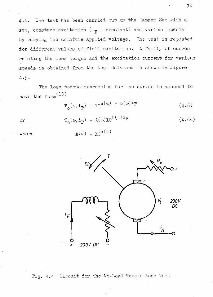
3 4
4.4. The test has been carr i e d out on the Tamper Set with a set, constant e x c i t a t i o n ( i j , = constant) and various speeds by varying the armature applied voltage. The test i s repeated f o r d i f f e r e n t values of f i e l d e x c i t a t i o n . A family of curves r e l a t i n g the lo s s torque and the e x c i t a t i o n current f o r various speeds i s obtained from the test data and i s shown i n Figure
The loss torque expression f o r the curves i s assumed to have the f o r m ^ 1 ^
4.5.
T (o),i p) 10' a ( t o ) + b(oo)i]p (4.6)
or A(LO)10 b(to)ip (4.6a)
where A(w) 10' a (to)
F
+ 230V DC -
F i g . 4.4 C i r c u i t f or the Ko-Load Torque Loss Test
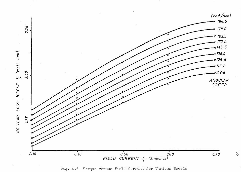
( rad/sec)
I , , , r— 0-30 0.40 0.50 0.60 0.70
FIELD CURRENT iF (amperes)
F i g . 4 . 5 Torque Versus F i e l d Current f o r Various Speeds

The torque-excitation current r e l a t i o n i s determined f i r s t f o r
each s p e c i f i c speed. By taking logarithms of equation (4.6)
there r e s u l t s
l o g T q = a(o>) + b(co)i p (4.7)
where oo = constant.
In order to determine the c o e f f i c i e n t s 'a' and 'b', i t
i s f i r s t required to divide the points along a curve into
approximately two equal groups i n successive order. Two
equations are then obtained by taking the sums of the i n d i v i d u a l
groups of values with the r e s u l t
m m
Z ( l o g T o ) ± = ma + ( Z ( i y ) ± ) b (4.8) i = l i = l
n n Z (log T Q ) k = na + ( Z ( i p ) k ) b , (4.9) k=l k=l
The two equations are then solved simultaneously to determine
the c o e f f i c i e n t s 'a' and 'b'. For example, 'a' and 'b' f o r
the speed of co = 188.5 rad/sec are determined from the data
given i n Table 4.1. Su b s t i t u t i n g the r e s u l t s of Table 4.1
int o equations (4.8) and (4.9)' and s o l v i n g f o r 'a' and 'b' gives
a = 0.194
b = 0.253
The value of 'A' obtained from equation (4.6a) i s
• A = 1.56
1 To obtain the complete l o s s torque expression as a
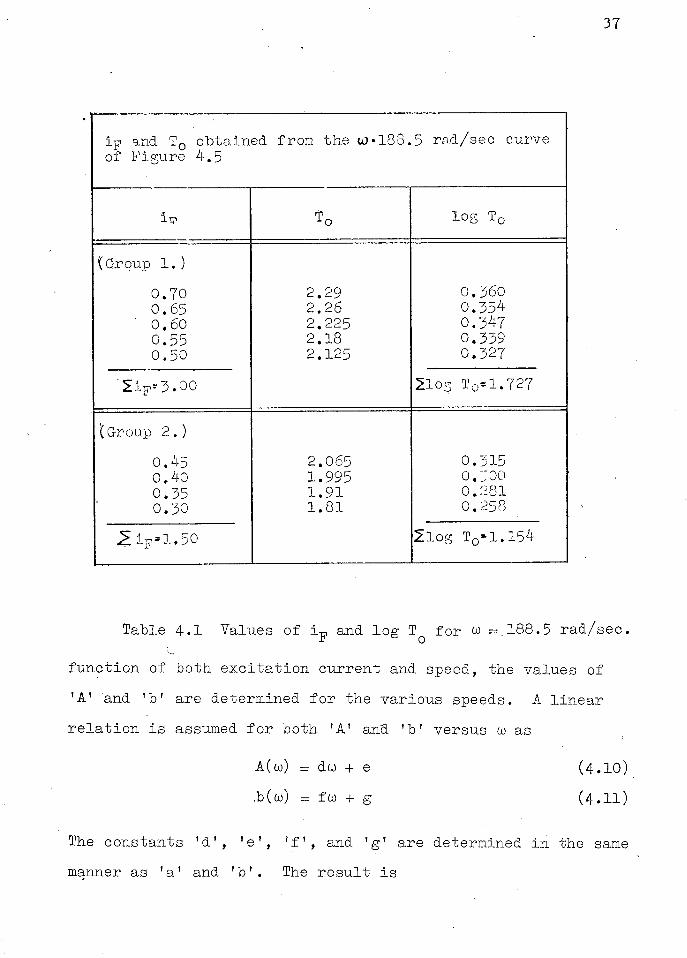
37
iv and T N obtained from the to• 1 8 8 . 5 rad/sec curve of Figure 4 . 5
iv To log T 0
(Group 1 . )
0 . 7 0 2 . 2 9 0 . 3 6 0
0 . 6 5 2.26 0 . 3 5 4
0 . 6 0 2 . 2 2 5 0 . 3 ^ 7
0 . 5 5 2 . 1 8 0 . 3 3 9
0 . 5 0 2 . 1 2 5 0 . 3 2 7
' £ iF- 3 . 0 0 2 1 os T 0 * 1 . 7 2 7
I Group 2 . )
0 . 4 5 2 . 0 6 5 0 . 3 1 5 0 . 4 0 1 . 9 9 5 0 . " 0 0
0 . 3 5 1 . 9 1 0 . 2 8 1
0 . 3 0 1 . 8 1 0 . 2 5 8
J ^ i p - 1 . 5 0 2 l o g T 0 = 1 . 1 5 4
Table 4 . 1 Values of i p and l o g T q for w = . 1 8 8 . 5 rad/sec.
function of both e x c i t a t i o n current and speed, the values of 'A' and 'b' are determined f o r the various speeds. A l i n e a r r e l a t i o n i s assumed f o r both 'A' an"d 'b' versus co as
A ( w ) = du + e ( 4 . 1 0 )
.b(w) = fw + g ( 4 . 1 1 )
The constants 'd 1, 'e', ' f , and 'g' are determined i n the same manner as 'a' and 'b'. The r e s u l t i s

38
A(co) = 1 .99«10"5
co + 1.18 ( 4 . 1 2 )
b(co) = 1 .39*10~4
co + 0 . 2 2 9 ( 4 . 1 3 )
The values of 'A' and 'b' f o r the various speeds are p l o t t e d
i n Figures 4.6 and 4.7 r e s p e c t i v e l y together with equations
( 4 . 1 2 ) and ( 4 . 1 3 ) .
The complete l o s s torque expression i s determined by
s u b s t i t u t i n g equation ( 4 . 1 2 ) and ( 4 . 1 3 ) into equation (4.6a)
with the r e s u l t
To(o),i
F) = ( l . 9 9 x l O -
3
c o + 1 . 1 8 ) l 0 ( l ' 3 9 x l 0 " 4 w + - 2 2 9 ) i F (4.
1 4 )
Since the dc motor i s constantly excited at 0 . 5 amperes
f o r the simulation and since the speed v a r i a t i o n e f f e c t on the
exponential i s small, equation ( 4 . 1 4 ) takes a l i n e a r form by
r e p l a c i n g co i n the exponential by the synchronous speed,' co =
188 .5 rad/sec
To(w , 0 . 5 ) = K co + K
2 ( 4 . 1 5 )
where = 2.67 x 1 0 ~ 5
K2 = 1 . 5 8 5
4.2.2 I n e r t i a of the Tamper Set
The i n e r t i a of the machine set i s determined by means
of a r e t a r d a t i o n t e s t . The t e s t has been c a r r i e d out by open
c i r c u i t i n g the armature of the dc motor running at synchronous
speed and monitoring the speed of the unit as a function of
time. With the l o s s torque expression, equation ( 4 . 1 4 ) , sub
s t i t u t e d i nto the torque equation ( 4 . 4 ) there r e s u l t s

39
1-60h
ISO
V40
1-30 100 120 140 160 180
ANGULAR SPEED (RAD/SEC)
F i g . 4 . 6 P l o t of 'A' v e r s u s 'to' and E q u a t i o n ( 4 . 1 2 )
0-260
0-250Y
0-240 100 120 140 160 180
ANGULAR SPEED (RAD/SEC)
200
F i g . 4 . 7 P l o t of 'b' v e r s u s 'co' and E q u a t i o n ( 4 . 1 3 )
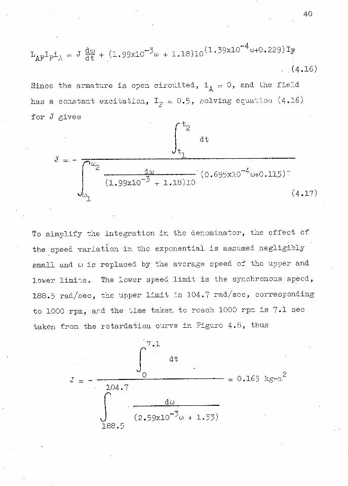
40
I ^ I p i ^ = J |^ + (l.99xlO- 3co + 1 . 1 8 ) l 0 ( l . 3 9 x l 0 - 4 a ) + 0 . 2 2 9 ) I p
• (4.16)
Since the armature i s open c i r c u i t e d , i ^ = 0, and the f i e l d
has a constant e x c i t a t i o n , Ip = 0.5, s o l v i n g equation (4.16)
f o r J gives
J =. -j i
dt
dec (1.99x10 3 + 1.18)10
' (0.695xlO"4o)+0.115)
co. '1 (4.17;
To s i m p l i f y the i n t e g r a t i o n i n the denominator, the e f f e c t of
the speed v a r i a t i o n i n the exponential i s assumed n e g l i g i b l y
small and co i s replaced by the average speed of the upper and
lower l i m i t s . The lower speed l i m i t i s the synchronous speed,
188.5 rad/sec, the upper l i m i t i s 104.7 rad/sec, corresponding
to 1000 rpm, and the time taken to reach 1000 rpm i s 7.1 sec
taken from the r e t a r d a t i o n curve i n Figure 4.8, thus
7.1
dt
J 0 = 0.165 kg-m^ 104.7
dco
(2.59x10 5 O J + 1.53; 188.5

41
200V
TIME (SECS)
P i g . 4.8 Retardation Curve for I n e r t i a Calculation
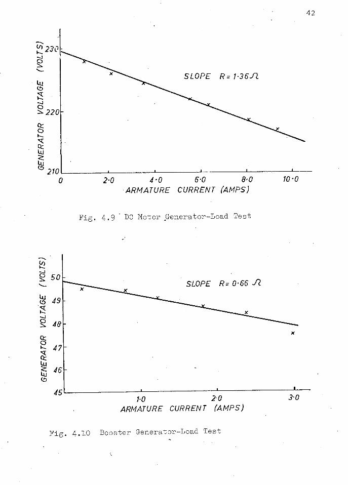
4•3 Resistance and Inductance Measurements
The armature resistances of both the dc motor and the (15)
booster have been determined from generator-load tests i n order to include the commutator and brush contact and temperature e f f e c t s . The graphs of generator voltage versus armature current are shown In Figures 4 . 9 and 4 . 1 0 for the dc motor and booster respectively. The armature resistances found from the slopes of the curves are
42
IJJ to 2701 L — >
0 2-0 4-0 6-0 8-0 10-0 ARMATURE CURRENT (AMPS)
F i g . 4.9 ' DC Motor G e n e r a t o r - L o a d T e s t
F i g . 4.10 B o o s t e r G e n e r a t o r - L o a d T e s t
43
R^ = 1.34-0- clc motor armature resistance
R =0.66-0- booster armature resistance a
The f i e l d resistance value of the booster, found at a room temperature of approximately 25°C using a General Radio Impedance Bridge, i s
R^ = 5 1 . 6 X 1 booster f i e l d resistance
Since the booster f i e l d current i s set at zero f o r the i n i t i a l operating condition and the f i e l d current due to the booster f i e l d voltage i s r e l a t i v e l y small compared with the rated value, the resistance i s deemed constant, independent of temperature.
The inductance of the booster and the dc motor armatures i n series and that of the booster f i e l d were determined by a
(15) transient current method ' . The test c i r c u i t i s shown i n Figure 4.11. The current response as a voltage across a known resistance R^ to a voltage step i s recorded on a Tektronix Storage Scope. The inductance i s calculated from the r e s i s t ance and the time constant of the c i r c u i t
1 = TR (4.18)
T = the time constant of the c i r c u i t R = R + R. = the resistance of the c i r c u i t .
The time required to reach 0'63(V m a x) a s shown on the scope i s 2.1 msec and the inductance of the booster and dc motor armatures connected i n series i s

44
Kt)
STEP
VOLTAGE WINDING <
STORAGE OSCILLOSCOPE
F i g . 4 . 11 Inductance Measurement C i r c u i t
L + L, = 7 ohms x 2 . 1 msec = 14 .7 mh
The constant for the booster f i e l d c i r c u i t i s obtained i n a more accurate manner by p l o t t i n g time versus l n ( i - i ( t ) ) as i n Figure 4 . 1 2 . v max °
3-0
25
i 2-0
I ^ 1-5
T= SLOPE=-^- =0-296 1-35
loo 200 300
TIME (MILL I SEC) -
400
F i g . 4 .12 Booster F i e l d Winding Current Response
45
The times and current values are obtained from the voltage transient across a known resistance. The inductance i s found
from ecuation (4.18) with the time constant obtained from Figure 4,12
I f= 87.1 ohms x 0.296 sec = 25.8 h
The resistance of the dc motor - booster armature c i r c u i t at f u l l load, including the load-setting r e s i s t o r ,
i s found to be approximately 10 fi . This gives an armature c i r c u i t time constant of
v ~ 14-7 mh = ± A 1 m s e c
10 ohms
Since the time constant Is very much smaller than any of the governor time constants, i t i s neglected i n the simulation. The time constant of the booster f i e l d , found from' i t s resistance and inductance values, i s

46
5 . TEST RESULTS
5 . 1 Analog Studies of Governor Representation and System Speed Responses
The machine acceleration equation, which has the f o r m
Tfflpn = G(p)H(p)(-n) - oc n - Am per unit ( 5 . 1 )
and the governor transfer function G(p), which has various forms depending on the type of governor and the s i m p l i f i c a t i o n s allowed, are set up on the Pace 231R Analog Computer and the speed response 'n' to a step load change 'Am' i s observed. The analog c i r c u i t of equation ( 5 . 1 ) i s shown i n Pigure 5 . 1
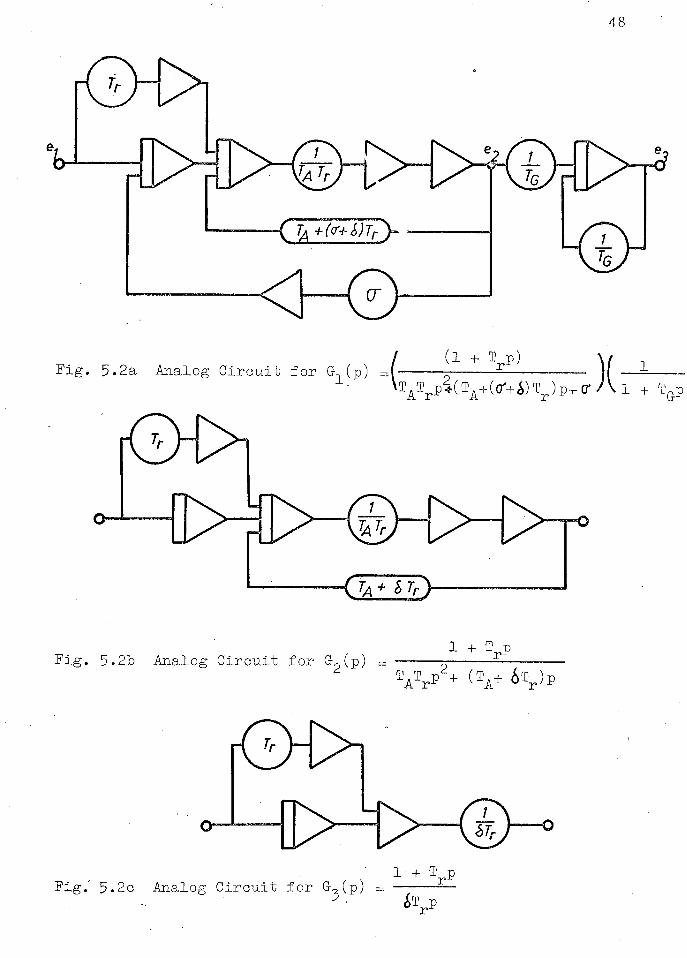
and the analog c i r c u i t d e t a i l s f o r the various governor transfer functions G(p) are given i n Figures 5 . 2 a through 5 . 2 c . The c i r c u i t f o r the hydraulic operator H(p) was given i n Figure 3 - 4 .
For the analog c i r c u i t of G- (p) , f or example, the set up i s obtained i n the following manner
1 + T p e 2 = ( e i) ( 5 . 2 )
(T AT rp 2 + (T A+(cr + 6)T r)p +<r)
or, re arranging
2 ~~ T.T ) 2 Ke2> 2 d A r ( p p p p ~ , c , s
and . e 3 = ~T + T Qp TfTT, ( e 2 ^ ( 5 . 4 )
47
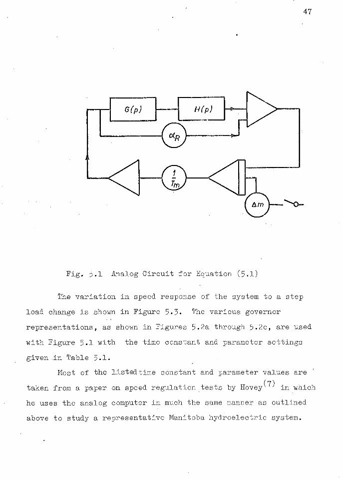
P i g . 5.1 Analog C i r c u i t f o r Equation (5.1)
The "variation i n speed response of the system to a step load change i s shown i n Figure 5.3. The various governor representations, as shown i n Figures 5.2a through 5.2c, are used with Figure 5.1 with the time constant and parameter settings given i n Table 5.1.
Most of the listedtime constant and parameter values are (7)
taken from a paper on speed regulation tests by Hoveyv i n which he uses the analog computer i n much the same manner as outlined above to study a representative Manitoba hydroelectric system.
4 8
F i g . 5.2a A n a l o g C i r c u i t f o r G. (1 + T p)
T A T r p i ( T A + ( c r + ^ ) T r ) p + c r / V i + T G p 1
1 + T p P i g . 5.2b A n a l o g C i r c u i t f o r G (p) = ----- r
2 " T A V 2 + (v
M > - ( S 1- + T p
F i g . ' 5.2c A n a l o g C i r c u i t f o r G„(p) = — 5 • p
49
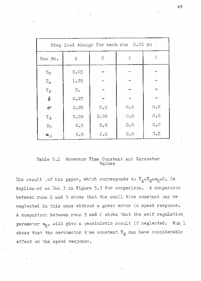
Step load change f o r each run 0 . 0 5 pu
Run No. 1 2 3 4
Tm 9 . 0 5 - - -Tw 1 . 2 5 - - -T r 5 . - - -b 0 . 2 ? - - -cr 0 . 0 5 0 . 0 0 . 0 0 . 0
T A 0 . 0 2 0 . 0 2 0 . 0 0 . 0
T G 0 . 5 0 . 0 0 . 0 0 . 0
«R 0 . 0 0 . 0 0 . 0 0 . 5
Table 5 -1 Governor Time Constant and Parameter Values
The r e s u l t .of h i s paper, which corresponds to TA=Tg_-<Xg=0, i s duplicated as Run 3 i n Pigure 5 . 3 for comparison. A comparison between runs 2 and 3 shows that the small time constant may be neglected i n t h i s case without a great error i n speed response. A comparison between runs 3 and 4 shows that the s e l f regulation parameter <x^, w i l l give a pessimistic r e s u l t i f neglected. Run 1
shows that the servomotor time constant can have considerable effect on the speed response.

F i g . 5.3 Speed R e s p o n s e t o a S t e p L o a d Change

51
5.2 Analog Study of the Prime Mover - Governor Model.
The prime mover - governor model, as outlined i n
Chapter 3, i s simulated on the Pace 231R Analog Computer using
system parameter values obtained i n Chapter 4 i n order to
examine i t s operation under steady state and transient con
d i t i o n s . The speed of the dc motor i s obtained from the torque
equation, (2.8), and set up on the computer as
Equation (5.5) together with the armature current equation
provide the necessary equations to set up the model on the
computer. The s e l f - r e g u l a t i o n c o e f f i c i e n t has been set equal
to zero.
The equations are amplitude scaled to some extent i n order
to maintain computer voltages within maximum l i m i t s and to avoid
high gain settings and the accompanying high noise l e v e l s .
Equation (5.5) i s s c a l e d by a fa c t o r of one h a l f to bring the
vari a b l e 'co' down to approximately the output of the dc tachometer
(5.5)
of the dc motor and booster, equation (2.6^,
(5.7)
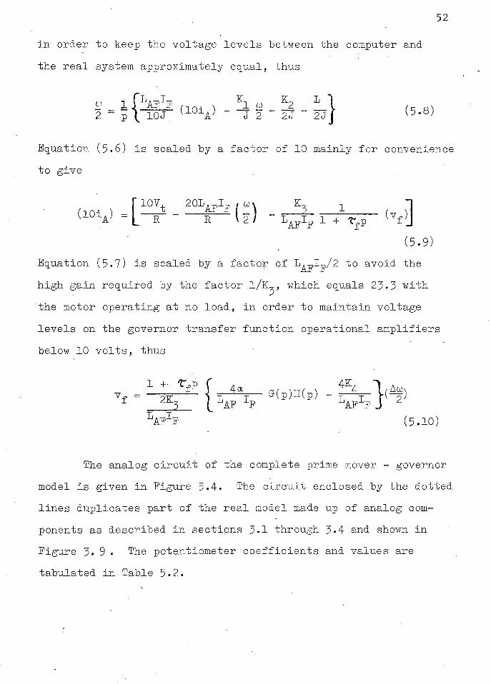
i n order to keep the voltage l e v e l s between the computer and the r e a l system approximately equal, thus
2 i ( W f l 0 i ) h a i L \ (. p.) p \ 1 0 J . U ° V " J 2 2 J " 2 J J ( 5 ' 8 )
Equation ( 5 . 6 ) i s scaled by a factor of 10 mainly for convenience to give
( l 0 l A ) = L " R S — l a / - iT± 1 + r , P
( v f } _ f l O V t 2 0 1 ^ , co ^ J L ,
JAF^"F ( 5 . 9 )
Equation ( 5 . 7 ) i s scaled by a factor of L^-pLp/2 to avoid the high gain required by the factor l/K^, which equals 23.3 with 'the motor operating at no load, i n order to maintain voltage l e v e l s on the governor transfer function operational amplifiers below 10 v o l t s , thus
j> { ""AE 1P - f = - 2 X 7 ^ - T~TT * < P > H ( P > - r V V(^) G(p)H(p) - T - V I ( ^ ) AF F J ^ " AF F ( 5 . 1 0 ;
The analog c i r c u i t of the complete prime mover - governor model i s given i n Figure 5 . 4 . The c i r c u i t enclosed by the dotted l i n e s duplicates part of the r e a l model made up of analog components as described i n sections 3-1 through 3-4 and shown i n Figure 3 . 9 . The potentiometer c o e f f i c i e n t s and values are tabulated i n Table 5 . 2 .

L
G(p)H(p) ) G(p)H(p)
FIL TER DIFFERENTIATOR
F i g . 5.4 Analog Setup of the Prime Mover - Governor Model
5 4
Load Level 3 0 ^ 50% 1 0 0 1
C o e f f i c i e n t s Settings
P62 10V t
R 130.0 155.0 2 2 5 . 5
F61 cO 2
9 4 . 2 5 - -
P60 I I J
0.0162 - -
E59 K2
2 J
0.048 - -P 5 8
L 2 J 3.35 5.21 10.42
P 5 5 4 *
LAp I
F
0.086 _ -P54 1>AF Iff
2 K 3
6.11 5.12 3 . 5 2
P51 4K4 L A F I F
0.209 0.247 . 0.353
2 0 LAJ P I F
R . 0 . 9 8 1.17 1.70
Q20 L A F : F 2J
0.257 — •*
Q15 1 t f
2.0 - -
Ql4 I C K 3
L A F x F * f 1.64 1.95 2.84
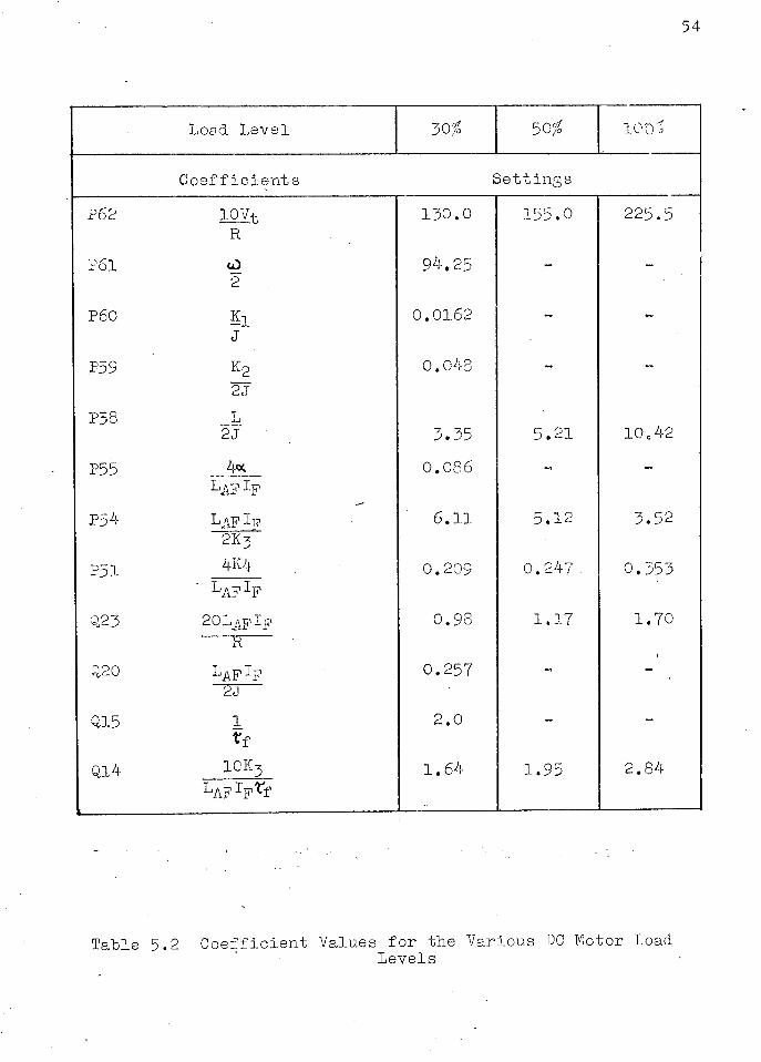
Table 5.2 Coefficient Values for the Various DC Motor Load Levels
55
5.3 Analog Study of the Model Response to a 30^ Step Load Rejection
The base load on the dc motor i s determined by the mechanical s t a r t i n g time of the system as shown i n equation (2.17). The operation of the model under step load changes i s examined on the analog computer using the c i r c u i t shown i n Figure 5.4 with the governor time constant and parameter values of Hovey as given i n Table 5.1.
The base load torque i s
acog = Y~ cog = c^Qcp x 188.5 = 3.44 nt-m
Steady state armature current-at f u l l load, calculated from the torque equation (2.8), i s
i. = T 1
T (K co + K + L)
= 75785 (2.09 + 3.44) = 6.51 amps
which i s w e l l w i t h i n the ratings of the dc motor. Table 5.2 gives the potentiometer settings f o r the
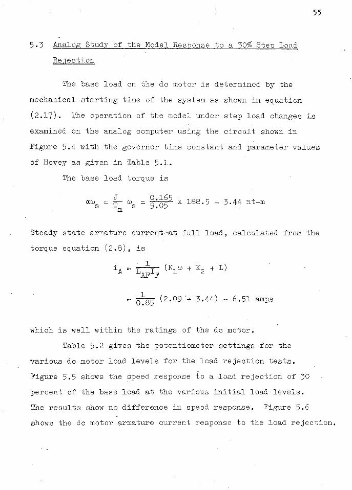
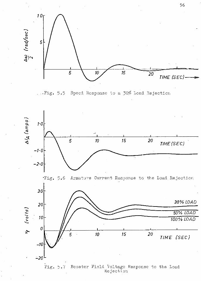
various dc motor load l e v e l s f o r the load r e j e c t i o n t e s t s . Figure 5.5 shows the speed response to a load r e j e c t i o n of 30 percent of the base load at the various i n i t i a l load l e v e l s . The r e s u l t s show no difference i n speed response. Figure 5.6 shows the dc motor armature current response to the load r e j e c t i o n .
56
. .-Pig. 5 . 5 Speed Response to a 30% Load Rejection
—20
F i g . 5 . 7 Booster F i e l d Voltage Response to the Load Rejection

57
While the current v a r i a t i o n response i s the same f o r the various load l e v e l s , the i n i t i a l current depends on the load. Figure 5.7 shows the booster f i e l d voltage responses to the 50 percent load r e j e c t i o n s . The magnitude of the response shows a decrease with the increase i n i n i t i a l load.
5.4 Real Model Tests
The actual model, shown schematically i n Figure 3 .9 , has been tested f o r steady state and load r e j e c t i o n .
Figure 5.8 shows the steady state A c o / 2 s i g n a l of the prime mover - governor model. The maximum speed error shown i s approximately 0.05 v o l t s i n 94.25 v o l t s .
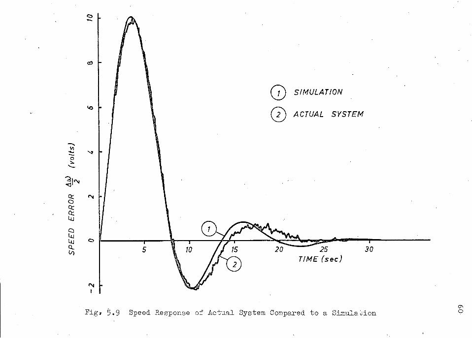
Figure 5.9 shows the transient speed response of the model" to a load r e j e c t i o n of '30 percent from an i n i t i a l load of 30 percent. The same governor as used by Hovey and mentioned i n section 5.1 and 5.2 has been set up on the s p e c i a l analog computer of the model fo r the t e s t . Run 1 shows the test r e s u l t with the dc motor, booster and load-setting r e s i s t o r simulated on the Pace Analog Computer and with the s p e c i a l analog computer of the model interconnected with i t . Run 2 shows the test run of the actual model including the s p e c i a l analog computer and the actual dc motor, booster and load-setting r e s i s t o r . The load i s obtained by loading the synchronous generator u n t i l the dc motor armature current reaches the predetermined value and Is rejected by open c i r c u i t i n g both the armature and f i e l d of the synchronous generator.
Figure 5.10 shows s i m i l a r load r e j e c t i o n test r e s u l t s .


59
In. t h i s case, however, the governor t r a n s f e r f unction as given
i n equation (5.5) has been used with a s e l f r e g u l a t i o n coef
f i c i e n t of a R = 1.0 and a permanent speed droop of <r=0.05.
It (5.5)
The time constants and parameter values are l i s t e d i n the
f i g u r e .
The curves of both Figures 5.9 and 5.10 show a d i s
crepancy i n period and amplitude -after the f i r s t swing between
the r e a l model and the analog. These discrepancies most
probably a r i s e as a r e s u l t of unavoidable errors i n the measure
ment of the dc motor and booster parameters and approximations
made i n the development of the model.
For the f i r s t few seconds a f t e r the load r e j e c t i o n , which
i s of primary concern i n transient power system studies, the
t e s t r e s u l t s of the model and the analog show very close
agreement.
F i g * 5.9 Speed Response of A c t u a l System Compared to a S i m u l a t i o n o

GOVERNOR
PARAMETERS
Tm = 9.26
Tr = 4.8
- F i g . 5.10 Speed R e s p o n s e o f A c t u a l S y s t e m Compared t o a S i m u l a t i o n
6. CONCLUSIONS
62
A prime mover - governor model has been designed,
constructed and tested as part of a new power system te s t
model. I t has been shown that i t i s capable of reproducing the
torque-speed c h a r a c t e r i s t i c of a large prime mover - governor
system. The model has been designed with a laboratory size dc
motor and a booster and i s capable of a t t a i n i n g the desired
response without the necessity of an adjustable flywheel as
required by previous micromachines.
Certain r e s t r i c t i o n s are placed on the model by the
equipment used. The maximum speed deviation i s l i m i t e d to
approximately 10 percent by the lOv operational a m p l i f i e r s
and the booster f i e l d voltage s i g n a l i s l i m i t e d to 60 v o l t s .
Test r e s u l t s i n d i c a t e that the model i s capable of carrying
out s t a b i l i t y t e s t s , up to f u l l load r e j e c t i o n f o r a few
seconds p r i o r to load r e a p p l i c a t i o n . Beyond the 10 percent
maximum speed deviation the model i s no longer v a l i d due to
system n o n l i n e a r i t i e s such as the nonlinear turbine character
i s t i c s mentioned i n Appendix I and r e l a y valve saturation
mentioned i n Appendix I I I .
The governing system of the present model i s capable
of r e s o l v i n g speed deviations of 0.05 percent. I t i s f e l t that
steady state performance can be improved through the use of a '
l e s s noisy and more accurate tachometer. With an improved
r e s o l u t i o n i n small speed de v i a t i o n s , nonlinear governor e f f e c t s
such as dead band and hysteresis may be incorporated into the
model i f required.
63
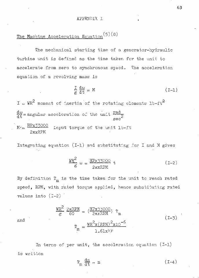
A P P E N D I X I
The Machine Acceleration- E q u a t i o n ^ ^
The mechanical s t a r t i n g time of a generator-hydraulic
turbine u n i t i s defined as the time taken f o r the unit to
accelerate from zero to synchronous speed. The a c c e l e r a t i o n
equation of a r e v o l v i n g mass i s
2 2 I = W R moment of i n e r t i a of the r o t a t i n g elements l b - f t
|TT = angular a c c e l e r a t i o n of the unit ra(^- . sec
m = z HPx55000 i n p u t torque of the unit l b - f t 2T C X R P M
Integrating equation ( I - l ) and s u b s t i t u t i n g f o r I and M gives
WR2 w = HPx55000 t ( T_ 2) g 2rtxRPM
By d e f i n i t i o n T i s the time taken f o r the unit to reach rated J m speed, RPM, with rated torque applied, hence s u b s t i t u t i n g rated
values i n t o (1-2)
WR2 2TCRPM _ /HPx55000> m g 60 ~ 1 2T C X R P M ; m
and ' ? ? r (!-3) T = WR x(RPM) xlO °
m ~ 1.6lxHP
In terms of per u n i t , the acc e l e r a t i o n equation ( I - l )
i s written
T ft = m (1-4) m dt

6 4
n = per unit angular speed m = per unit input torque
(Q) Ine per unit incremental turbine torque i s written as '
where g = per unit r e l a t i v e instantaneous gate change h = ',' " " " head " n = " 11 11 " speed "
and the p a r t i a l derivatives are the slope constants of the nonl i n e a r turbine c h a r a c t e r i s t i c s . For the i d e a l turbine operating at the point of best e f f i c i e n c y ^ , equation (1-5) i s given as
m = g + 1.5h - ct^n (1-6)
where ocR i s the c o e f f i c i e n t of net s e l f - r e g u l a t i o n of the turbine and load and has a value range of 0 to 1. Including a per unit step load change and s u b s t i t u t i n g equation ( 1 - 6 ) , equation (1-4) i s written
Tm I t = g + 1 ' 5 h ~ V 1 " ^ ( I _ 7 )
where Am i s a per u n i t step load change. The r e l a t i o n s h i p s between 'g', 'h' and 'n' follow i n Appendices I I and I I I .

65
APPENDIX I I
(5) The Water Acceleration Equation and Hydraulic Operator
The derivation of the transfer function r e l a t i n g gate changes to per unit head changes i s based on the following assumptions: a) conduits (penstock, s c r o l l case and draft tube) are i n e l a s t i c b) water i s incompressible c) flow i s f r i c t i o n l e s s d) water v e l o c i t y i s proportional to the square root of the
net turbine head and d i r e c t l y proportional to the gate opening
Erom the l a s t assumption
U = water v e l o c i t y H = net turbine head G = gate opening Z = a constant For small displacements from an operating point
U = K v A H ^ * G ( n - i ) .
AU = K N / I T - AG + i 1 KAHG ( H - 2 ) 2
jr
In per unit
U " = 2 H o o AU 1 AH
+ AG G ( H - 3 ) o

66
- Since a decrease i n flow i n the turbine with gate 'closure*results i n an increased pressure, or e f f e c t i v e head, due to the water column i n e r t i a , the water acceleration i s written as
f L A <Mff = -A_p gAH ( I I-4)
where j> = mass density of the water A = cross section of the water passage L = t o t a l length of the water passage g = g r a v i t a t i o n a l constant In terms of per u n i t , equation (-II-4) becomes
m. U M)_ ( I I_ 5 ) & O O 0
The t o t a l water s t a r t i n g time i s defined by
T = w gH & o
The summation i s required since the water passage has a variable cross section and, as a r e s u l t , a variable water v e l o c i t y . 5 D i f f e r e n t i a t i n g equation ( I I - 3 ) , m u l t i p l i e d .by Tw, and using the following notation
u = per unit v e l o c i t y change o
g = — per unit gate change o
h : per unit head change o

67
equation (II-3) becomes T
T ft = -4 ft -,. T | f (II-6) w dt , 2 dt ' w dt v
Substituting equation (II-6) into equation (II-5) and using the per unit notation
T 'w dh + ft (II-7) ~ h ~ 2 dt + "w dt
which gives the r e l a t i o n between 'h' and 'g'. The hydraulic operator, H(p), i s obtained by sub
s t i t u t i n g equation (II-7) into the torque term i n equation (1-7) thus
/ 1 - T p \ f I \ g _ £v n _ Am (II-8) V I + 0.5 T p /
rp dn m d t v^ + 0.5 T p
w 1 - T p
where " hydraulic operator, H(p). 1 + 0.5 \ p

68
APPENDIX I I I
The Mechanical Governor Transfer Function V J"' 1
Appendix I I I r e l a t e s the derivation of the governor transfer function f o r the arrangement shown schematically In Figure I I I - l .
Consider f i r s t the r e l a t i o n between the p i l o t valve movement and the actuator piston movement. The v e l o c i t y of the actuator piston i s proportional to the p i l o t valve p o s i t i o n as long as the p i l o t valve p o s i t i o n does not cause the piston v e l o c i t y to saturate. From Figure I I I - 2 , the r e l a t i o n s h i p between p i l o t valve p o s i t i o n and piston v e l o c i t y i s
dx' x x < p ( I I I - l ) dt ~ 'A
where T. = 1 actuator time constant.
F i g . III.2 Plot of Actuator Piston Velocity Versus P i l o t Valve P o s i t i o n

69
FLYBALLS
PILOT VALVE
GATE SERVOMOTOR
J i g . I I I . l Schematic Diagram of a Mechanical H y d r a u l i c Governor
70
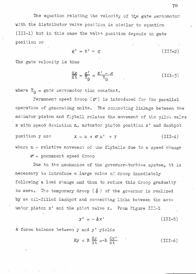
The equation r e l a t i n g the v e l o c i t y of the gate servomotor
w i t h the d i s t r i b u t o r v a l v e p o s i t i o n i s s i m i l a r to equation
( I I I - l ) but i n t h i s case the v a l v e p o s i t i o n depends on gate
p o s i t i o n or .
g* = x' - g ( I I I - 2 )
The gate v e l o c i t y i s thus
where T^ - gate servomotor time constant.
Permanent speed droop (<T) i s introduced f o r the p a r a l l e l
o p e r a t i o n of g e n e r a t i n g u n i t s . The connecting l i n k a g e between the
a c t u a t o r p i s t o n and f l y b a l l r e l a t e s the movement of the p i l o t v a l v e
x w i t h speed d e v i a t i o n n, a c t u a t o r p i s t o n p o s i t i o n x' and dashpot
p o s i t i o n y a s : x = n + < r x ' + y ( I I I - 4 )
where n = r e l a t i v e movement of the f l y b a l l s due to a'speed change
a* = permanent speed droop
Due to the mechanics of the'governor-turbine system, i t i s
necessary to i n t r o d u c e a l a r g e value of droop immediately
f o l l o w i n g a l o a d change and then to reduce t h i s droop g r a d u a l l y
to z e r o . The temporary droop ( $ ) °f the governor i s r e a l i z e d
by an o i l - f i l l e d dashpot and connecting l i n k s between the a c t
uator p i s t o n x' and the p i l o t v a l v e x. Prom Figure I I I - l
y* = - 6x- ( H l - 5 )
A f o r c e balance between y and y' y i e l d s
71
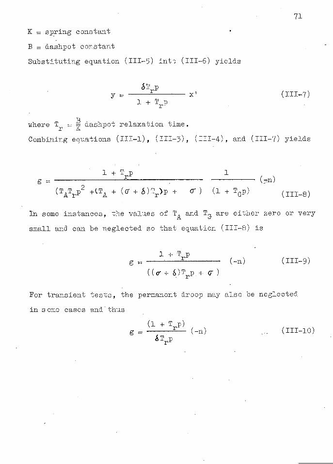
K = s p r i n g constant
B = dashpot constant
S u b s t i t u t i n g equation ( I I I - 5 ) i n t o ( I I I - 6 ) y i e l d s
1 + T rp
where I - ^ dashpot r e l a x a t i o n time.
<$T p y = ~ x- ( I I I - 7 )
r ~ K Combining equations ( I I I - l ) , ( I I I - 3 ) , ( I I I - 4 ) , and ( I I I - 7 ) y i e l d s
1 + T p 1 £ . (-_n) ( T A T R P 2
+ c i A + (cr + «S)iy>P + <r ) ( i + T GP) ( I I I _ 8 )
In some i n s t a n c e s , the valu e s of T A and T & are e i t h e r zero or very
s m a l l and can be neglected so t h a t equation ( I I I - 8 ) i s
1 + T p g = = r ( _ n ) ( I I I - 9 )
((a- + 6)T RP + <7 )
For t r a n s i e n t t e s t s , the permanent droop may a l s o be neglected
i n some cases and'thus
(1 + T p) g = (-n) ... (111-10)

72
1 Stevenson, W.D., Elements of Power System A n a l y s i s , McGraw-Hill, 1962, Ch 10.
2. Robert, H. , Micromachines and Uicroreseaux: Study of the Problems of Tr a n s i e n t S t a b i l i t y by the Use of Models S i m i l a r E i e c t r o m e c h a n i c a l l y to E x i s t i n g Machines and Systems, C.I.G.U.E., V o l . I l l , No. 338, 1950.
3. Venikov, V.A., Representation of E l e c t r i c a l Phenomena on P h y s i c a l Models as A p p l i e d to Power System Design, C.I.G.R.E., V o l . I l l , No. 339, 1952.
4. Adkins, B., Micromachine Studies at Imperial C o l l e g e , . E l e c t r i c a l Times, J u l y 7, I960.
5 . Hovey, L.M., and Bateman, L.A., Speed Regulation Tests on a Hydro S t a t i o n Supplying an I s o l a t e d Load, AIEE Transa c t i o n s , p t . I l l , V o l . .81, Oct. 1962, pp 364-368.
6 . Concordia, C , and Kirchmayer, L.K., Tie-Line Power and Frequency Con t r o l of E l e c t r i c Power Systems, AIEE T r a n s a c t i o n s , p t . I l l , V o l . 72, June 1953, pp 562-573.
7 . Hovey, L.M., Optimum Adjustment of Governors i n Hydro Generating S t a t i o n s , Engineering I n s t i t u t e of Canada, Nov. 1960, pp 64 - 7 1 .
8. Paynter, H.M., and Vaughan, D.R., Discussion of Speed R e g u l a t i o n Tests on a Hydro S t a t i o n Supplying an I s o l a t e d Load by Hovey and Bateman, AIEE Transactions, pt. I l l , V o l . 81, Oct. 1962, pp 368-369.
9. Paynter, H.M., D i s c u s s i o n of T i e - L i n e and Frequency C o n t r o l of E l e c t r i c Power Systems - Part I I by Concordia and Kirchmayer, AIEE Transactions, V o l . 73, A p r i l 1954, pp 141-144.
10. P h i l b r i c k Researches Inc., A p p l i c a t i o n s Manual f o r Computing A m p l i f i e r s f o r M o d e l l i n g , Measuring, M a n i p u l a t i n g , and Much E l s e , George A. P h i l b r i c k Inc., June 1966, pp 74-75.
11. I b i d , pg 49. 12. Bond, J . , A S o l i d State Voltage Regulator and E x c i t e r f o r
a Large Power System Test Model, U.B.C. MASc. Thesis, J u l y 1967, pp 9-11.
13. F i t c h e n , F.C., T r a n s i s t o r C i r c u i t A n alysis and Design, D. Van Nostrand Co., Dec. 1963, pg 79.

73
1 4 . Daws o n , G . E . , M o d e l l i n g , A n a l o g u e and T e s t s o f an E l e c t r i c M a c h i n e V o l t a g e C o n t r o l S y s t e m , U . B . C . MASc. T h e s i s , S e p t . 1 9 6 6 , page 1 1 .
1 5 . I b i d , pp 7 - 8 .
16. D a v i s , D . S . , Nomography and E m p i r i c a l E q u a t i o n s , J i e i n h o l d P u b l i s h i n g C o . , 1 9 5 5 , Ch 1.
1 7 . R i c h , G . R . , H y d r a u l i c T r a n s i e n t s , D o v e r P u b l i c a t i o n s C o . , 1 9 6 3 , Ch 3 .