a preliminary study of food court analytics
TRANSCRIPT

The Pennsylvania State University
The Graduate School
College of Engineering
Department of Industrial and Manufacturing Engineering
A PRELIMINARY STUDY OF FOOD COURT ANALYTICS
A Thesis in
Industrial Engineering
by
Arunachalam Arunachalam Palaniappan
2014 Arunachalam Arunachalam Palaniappan
Submitted in Partial Fulfillment
of the Requirements
for the Degree of
Master of Science
May 2014

ii
The thesis of Arunachalam Arunachalam Palaniappan was reviewed and approved* by
the following:
Soundar Kumara
Allen E. Pearce/Allen M. Pearce Professor
Professor of Industrial Engineering
Thesis Adviser
*Signatures are on file in the Graduate School
Christopher Saldana
Assistant Professor of Industrial Engineering
Paul Griffin
Peter and Angela Dal Pezzo Department Head Chair
Professor of Industrial Engineering
Head of the Department of Industrial and Manufacturing Engineering

iii
ABSTRACT
Embedded software packages have revolutionized the field of data collection, assimilation
and associated analytics through the ease of visualization tools such as customized report
generation and plug-and-play dashboards. The impact of this though far-reached is largely left
unexplored in the food industry where opportunities to optimize end-to-end data collection,
processing and management could potentially have a multi-fold impact.
Information is critical for making decisions, and communication of this information is harder as
the attention span of people has been reduced due to the speed with which the world is moving
today. Thus newer approaches like dashboards in data visualization are used to convey large
amount of information in a constrained display. In this thesis, we will explore how the food court
management can monitor the customer, employees and the restaurants through some components
of a dashboard. We shall discuss an optimization model that will create an optimal schedule for
employees so that they are used only during their most productive hours. Next we shall rank the
restaurants based on sales, number of visitors and number of revisits to understand how each
restaurant is doing compared to others. Two other analyses is on customer summary to generate
insights about the customers and association rule mining to see the rules for items being bought
together.
This information inferred can be used to make recommendations like, how much the customers
should refill the card for so that they can avoid entering the queue for multiple refills, the
customers can be recommended new food options that they might be interested in based on their
previous purchases, and management can use these association rules to make marketing
strategies and generate coupons. Another application for these analytics is to schedule employee
shifts based on traffic and make sure the employees are not over worked and they are at the peak
of their performance to serve the customers to the best of their ability.

iv
TABLE OF CONTENTS
List of Figures .......................................................................................................................... .vi
List of Tables ........................................................................................................................... vii
Acknowledgements……………………………………………………………………….....viii
Chapter 1 Introduction ............................................................................................................. ..1
1.1 Overview .................................................................................................................... ..1
1.2 Background and Motivation ....................................................................................... ..2
1.3 Problem Statement ..................................................................................................... ..3
1.4 Research Objectives ................................................................................................... ..4
1.5 Thesis Structure .......................................................................................................... ..5
Chapter 2 Literature Review .................................................................................................... ..6
2.1 Data Mining ............................................................................................................... ..6
2.2 Associative Rule Mining Algorithms ......................................................................... ..8
2.3 Data Analytics in Retail and Restaurant Industries .................................................... 11
Chapter 3 Database Structure ................................................................................................... 14
3.1 Current Database Design ............................................................................................ 15
3.2 Proposed Database Design ......................................................................................... 16
Chapter 4 Analysis and Results ............................................................................................... 19
4.1 Employee Scheduling................................................................................................. 20
4.1.1 Step 1: Service Rate Calculation ..................................................................... 21
4.1.2 Step 2: Optimization Model ............................................................................ 23
4.2 Restaurant Ranking .................................................................................................... 26
4.2.1 Net Sales per Day ............................................................................................ 27
4.2.2 Footfall ............................................................................................................ 28
4.2.3 Revisits ............................................................................................................ 29
4.3 Customer Summary .................................................................................................... 30
4.3.1 Customer Name ............................................................................................... 32
4.3.2 Total Purchase ................................................................................................. 32
4.3.3 Average Balance ............................................................................................. 33
4.3.4 Most Frequent Items Bought ........................................................................... 33
4.3.5Current Balance ................................................................................................ 34
4.3.6 Average Refill Amount ................................................................................... 35
4.3.7 Number of Visits ............................................................................................. 36
4.3.8 Average Discount Earned ................................................................................ 36
4.3.9 Most Recent Restaurant Visited ...................................................................... 37
4.3.10 Last Purchased Item ...................................................................................... 37
4.3.11 Most Visited Restaurant(s) ............................................................................ 38
4.3.12 Net Purchase by Restaurant ........................................................................... 38
4.4 Association Rule Mining ............................................................................................ 39
4.4.1 Apriori Algorithm ........................................................................................... 40
4.5 Clustering Analysis .................................................................................................... 43
v
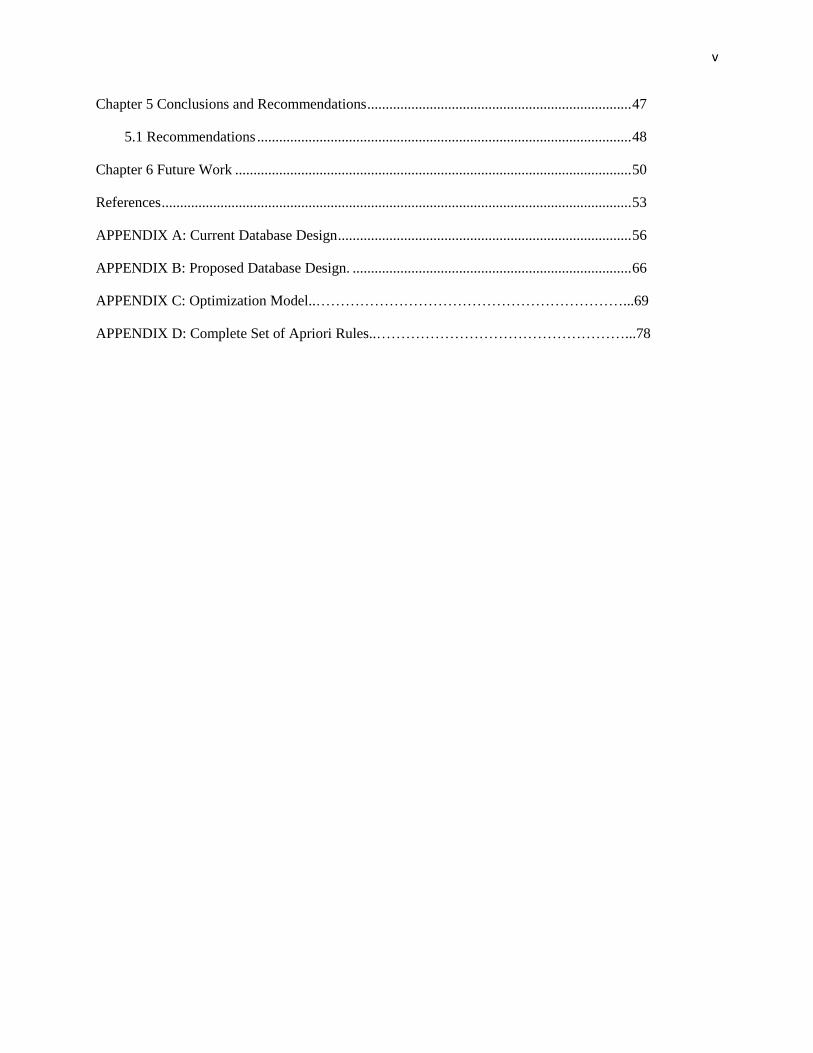
Chapter 5 Conclusions and Recommendations ........................................................................ 47
5.1 Recommendations ...................................................................................................... 48
Chapter 6 Future Work ............................................................................................................ 50
References ................................................................................................................................ 53
APPENDIX A: Current Database Design ................................................................................ 56
APPENDIX B: Proposed Database Design. ............................................................................ 66
APPENDIX C: Optimization Model..………………………………………………………...69
APPENDIX D: Complete Set of Apriori Rules..……………………………………………...78

vi
LIST OF FIGURES
Figure 4.1 Service rate for each employee for every operational hour .................................... 22
Figure 4.2 Employee Schedule for maximum service ............................................................. 25
Figure 4.3 Net Sales per day for all the twenty restaurants ..................................................... 28
Figure 4.4 Footfall for all the twenty restaurants ..................................................................... 29
Figure 4.5 Revisiting customer for each restaurant ................................................................. 30
Figure 4.6 Balance after each refill. ......................................................................................... 34
Figure 4.7 Refill Amount during each refill visit ..................................................................... 35
Figure 4.8 K-Mean clustering results visualized in 3-D .......................................................... 45
vii
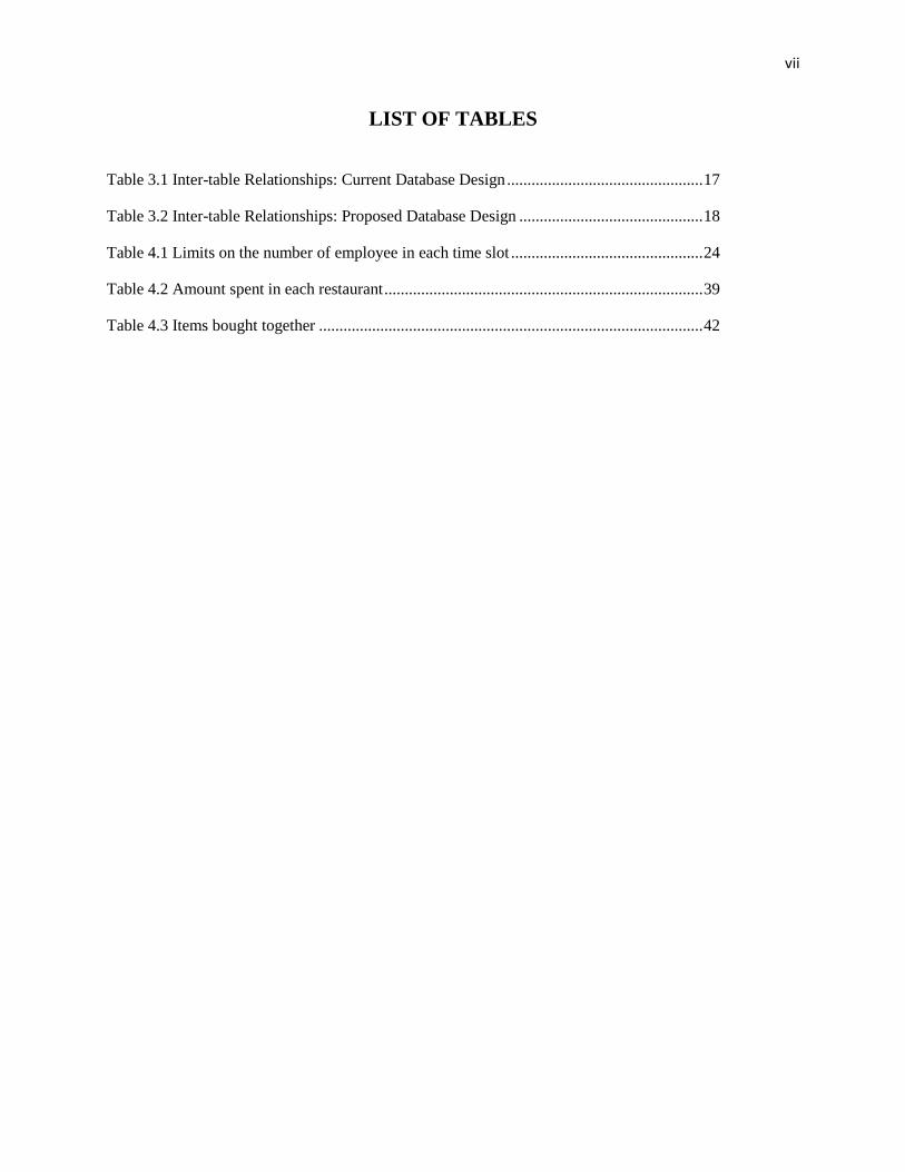
LIST OF TABLES
Table 3.1 Inter-table Relationships: Current Database Design ................................................ 17
Table 3.2 Inter-table Relationships: Proposed Database Design ............................................. 18
Table 4.1 Limits on the number of employee in each time slot ............................................... 24
Table 4.2 Amount spent in each restaurant .............................................................................. 39
Table 4.3 Items bought together .............................................................................................. 42

viii
ACKNOWLEDGEMENT
I would like to express my sincere gratitude for my advisor Dr. Soundar Kumara for being a
remarkable advisor and providing me moral support. I would like to thank him for his patience
and mentorship throughout my thesis at Penn State . His advice has been invaluable and I am
always indebt to him. He introduced me to the world of analytics which inspired this thesis. I
would also like to thank Dr. Paul Griffin and Dr. Christopher Saldana for their time and effort to
read my thesis and provide me with comments and suggestions to improve it. I would like to
thank my colleague Cheng-Bang Chen, Donghuan Tang for their tips to help me complete my
thesis. Lastly I would like to thank my parents and grandparents for their never-ending love,
financial support, and guidance.
Thank you Penn State for making me a world class engineer !

1
Chapter 1
Introduction
1.1 Overview
With fast growth in information technology, pace of data collection has increased in the past
decade. Data is collected about everybody everywhere, but only 2% of the information is used to
affect change and drive results. With more information being available for research, the
capabilities of extracting better insights from data has become easier. Many of the manual
processes have been replaced by automated software which does it in a click of a button and with
less effort from the user [Kohavi, 2002]. Few years ago, data being collected had considerable
anomalies and errors which made automation difficult. But with newer software these errors and
anomalies can be fixed automatically with business rules that the user defines, thus making
analytics much more accessible for everybody.
Analytics is a method by which meaningful patterns in data can be generated and communicated
to the user. There are numerous ways to find meaningful patterns, some of the methods include,
data mining, predictive modeling, machine learning, and neural networks. Analytics relies on
accessing data and applying various concepts of statistics, computer programming and operations
research to analyze the data and identify useful information [Fayyad,1996]. In recent years,
communication of these results has been harder as people, especially business users, do not have
the patience to read documents and reports. They want to look at colorful charts and graphs
instead of black and white documents. Thus communications of these business insights have
opened up paths to data visualization.

2
Data visualization is a means through which abstract information in the form of variables and
attribute can be communicated through graphical methods [Friedman, 2008]. The graphical
methods consist of bar, pie and line charts, tree maps, heat maps, etc. Depending on the user
different methods are chosen to represent the data. Newer methods include interactive graphs
where the user can filter huge amount of data to certain variables they are interested in at that
moment. Sometimes one graph or figure cannot represent the current status of a business, thus
they use dashboards. Dashboards are a collection of these graphical methods to represent the key
performance indicators of the business that is presented in one display.
1.2 Background and Motivation
Food industry is a fairly stable industry which has a steady growth potential. But unfortunately
analytics has not reached this far in this industry like retail, e-commerce, banking etc. Similar to
other industries there are customers who buy the products and vendors that sell them, and every
time a transaction occurs it is recorded to have a digital foot print. In the past, the usefulness of
this information goes as far as forecasting the next month sales using historical averages. This
vast data can be used to revolutionize the customer experience when they walk into a restaurant.
In an effort to achieve excellent customer experience, data from a food court in India was
collected. This food court has 20 restaurants across 15 different cuisines, like North Indian,
South Indian, South Asian, American, and other specialty restaurants. Each day this food court
serves over 1000 customers (one customer might be a single individual, a couple or a family) the
food choice they like. Each customer spends about Rs. 500 on an average every time they visit
the food court. A customer might have multiple transactions per visit thus the average number of
transactions recorded per day is about 3000. The food court keeps track of its customers and their

3
purchases through a card that the customer uses to purchase the item. This card is called a debit
card as the customer can fill it with money any time and spend it throughout the food court, very
similar to actual bank issued debit card, once the money is exhausted they need to refill before
using it again.
This food court collects a large amount of data about the customer and their purchases but
unfortunately they do not use this information to help increase sales or attract new customers.
The data is rich in information as we can track every movement of a customer in the food court
and use it to predict future events. This information can be shared with the restaurants to help
them better market themselves to the customers, or maybe even start profiling the customer into
segments or groups for marketing purposes. This thesis uses this information to make
recommendations to food court management and display the results of the analysis in the form of
a dashboard which is easily understood by them.
1.3 Problem Statement
The problems that are being addressed in this thesis are
Problem 1: Database Redesign
The database in the food court is filled with redundant tables, duplicate columns, and
unnecessary information that are not being collected (empty columns). Due to this the number of
tables needed to store the information is significantly more. As a result when conducting analysis
these tables and information cause errors and lags. Thus we need to redesign the database to
avoid these redundant tables and still maintain data integrity.

4
Problem 2: Food Court Analytics
Currently the food court management has no visibility on what the customer buys and what the
customer prefers. The management is unable to use the information collected in the database to
help improve the customer’s experience. The employees of the food court do not know what to
recommend the customers if they come for advice. The food court management does not know
what kind of promotions or coupons the customers will prefer. To help them address these issues
analytics can be used.
1.4 Research Objectives
The major objectives of this thesis are
1. To redesign the food court database to help reduce redundant data and maintain data
integrity.
2. To build a framework for analytics to study customer buying patterns, identify promotion
points and generate visualizations.
In the analytics part this thesis focuses on the following five components:
1. Employee Scheduling
2. Restaurant Ranking
3. Customer Summary
4. Association Rule Mining
5. Clustering Analysis

5
1.5 Thesis Structure
This thesis is organized into six chapters. Chapter 1 introduces the problem and the motivation
for this thesis. Chapter 2 is literature review where some of the papers that talk about analytics,
optimization, food industry and data mining are reviewed and discussed. Chapter 3 is about the
database structure, and deals with the data collection and how it is stored and in the end a new
design is proposed to solve some of the problems with the current database. Chapter 4 is on the
analysis and results, here each of the methods are explained in detail and the results are presented
as well. Chapter 5 details conclusion and results, where all the information is summarized and
some recommendation for the management are presented. The last Chapter 6 deals with future
work.

6
Chapter 2
Literature Review
Literature reviewed for the purpose of this thesis has been classified into three parts: Data
mining, Associative rule mining algorithms, and Data analytics in retailer and restaurant
industry.
2.1 Data Mining
Data mining has many papers and many methodologies, but for this thesis the following two
papers were studied for the application of data mining in newer fields like social networks, and
customer networks.
Wang et al. [2011] defined and explored community kernel detection in order to uncover the
hidden community structure in large social networks. They formulated the problem of
community kernel detection in large social networks as two subtasks: identifying influential
(kernel) members and detecting the structure of community kernels. Wang et al. [2011] proposed
GREEDY and WEBA, two efficient algorithms for finding community kernels in large social
networks. GREEDY is based on maximum cardinality search, while WEBA formalizes the
problem in an optimization framework. . They validated the effectiveness and efficiency of the
two algorithms on three large social networks: Coauthor, Wikipedia, and Twitter. Experimental
results showed that WEBA and GREEDY outperforms eight other state-of-the-art methods for
detecting community kernels. WEBA achieved an average 15%–50% performance improvement
over the other state-of-the-art algorithms, and WEBA is on average 6–2,000 times faster in
detecting community kernels. GREEDY also achieved a better performance than comparative

7
algorithms, but on average works 10% and 7% less well than WEBA. Wang et al. [2011] also
evaluated the efficiency performance and scalability of GREEDY and WEBA by comparing
their computational time required to detect community kernels with that of other algorithms on
the Coauthor, Wikipedia, and Twitter networks. Results from experiments proved that both
WEBA and GREEDY significantly reduced the required CPU time compared with the other
algorithms. Further, the CPU time required by WEBA and GREEDY increased almost linearly
with respect to the number of vertices, the density, and the kernel size, which demonstrated the
algorithms high scalability. Their qualitative case study on the Twitter network demonstrated the
ability of WEBA to find meaningful community kernels, which revealed the common profession,
interest, or popularity of groups of influential individuals. The successful detection of
community Kernels has many practical applications, including representative user finding, friend
recommendation, network visualization, and marketing.
Shaw et al. [2001] explored the situation of Organizations having large volumes of data on their
customers, which had created opportunities as well as challenges for Organizations to leverage
the data in order to utilize them efficiently and gain a competitive advantage. They advocated
that data mining tools can help uncover the hidden knowledge and understand customers better,
while a systematic knowledge management effort can channel the knowledge into effective
marketing strategies. They explored the study of the knowledge extraction and management and
its value for marketing. Michael Shaw and team emphasized the critical role played by marketing
decisions in today’s customer-centric environment. They proved how data mining can be
integrated into a marketing knowledge management framework for efficient knowledge
discovery and management. They utilized large volume of data and overcame the challenge of
filtering, sorting, processing, analyzing and managing this data in order to extract the information

8
relevant to the user. A systematic application of data mining techniques enhanced the knowledge
management process and equipped the marketers with better knowledge of their customers
leading to better service to customers.
2.2 Associative Rule Mining Algorithms
Data mining is a novel technique used to make sense out of data. Data mining algorithms
essentially perform two operations: (i) generate associative rules with strong support, from a
given data set to relate different data entities (ii) generate classifiers that divide data sets into
groups. The papers discussed below are different ways in which associative rule mining can be
used and how it can be combined with other mining tools get better results.
Lin et al. [2002] proposed an associative rule-mining algorithm for collaborative recommender
systems. The purpose of collaborative recommender systems is to personalize e-commerce by
studying similarities and dissimilarities among different customers. The existing associative rule
mining algorithms were designed for market basket analysis with an input support value. The
algorithm takes confidence as input to report rules. The algorithm is broken down into outer loop
and inner loop. The outer loop is called Main process that varies threshold support such that
minimum confidence constraint is met. The support generated in outer loop is input into inner
loop, which mines data using a variant of Apriori algorithm. Each article in database is given a
score, which is sum-product of support and confidence for all rules. Their experimentation shows
significant improvement in associative rule identification compared to traditional algorithms.
However the authors find that mining of large number of rules takes extremely long and does not
add value to recommendations.

9
Liu, Hsu and Ma [1998] proposed a new effort to integrate classification and association rule
mining techniques. They suggested an algorithm that builds classifiers based on class association
rules (CARs) generated using algorithms in literature. These CARs satisfy support and
confidence constraints. The authors propose CBA-RG algorithm to generate association rules
and CBA-CB algorithm to generate classifiers. The CBA-RG algorithm is explained as follows.
The algorithm generates all frequent ruleitems by making multiple pass over data. A ruleitem
consists of a set of items and a class label. In successive passes the ruleitems that are frequent are
passed on to the next pass. Frequesnt ruleitems are defined as ruleitems with minimum support
threshold and minimum confidence threshold. The support and confidence of a ruleitem are
computed using formulae shown below.
Support = Rulesupcount*100/|D|
Confidence = Rulesupcount*100/Condsupcount
Where: |D| is cardinality of dataset, Rulesupcount is support count of ruleitem and Condsupcount
is support count of all items in the ruleitem. The CBA-CB algorithm generates classifiers as
follows. The algorithm ranks all rules in decreasing order of confidence. In case of equal
confidence, support is used as a tiebreaker. Then each rule is applied to dataset D and those cases
covered by rule are removed from D. Then the classification error is measured. If the error does
not meet threshold, the next rule in the list is used to classify the updated D. This is repeated
until all items in D are classified. The authors find that classifier generated in experiments was
found to be more accurate than ones generated by then state of the art classification systems. The
disadvantage of the classification algorithm is that it does not use training set to learn but uses
entire dataset. Hence this algorithm cannot be used for dynamic applications where learning with

10
every update in dataset is necessary. The algorithm has to be run for entire dataset for every
update, making it computationally inefficient.
Hipp et al [2000] provide a survey of several efficient algorithms that accomplish association
rule mining. An association rule is a method for the discovery of unique relationships between
two or more variables in a dataset of considerable size. The paper describes a challenge in
association rule mining in that there are an immense number of rules that can be theoretically
considered, and the rate at which it grows is exponential. Hence a minimum threshold known as
minsupp is defined with respect to which all itemsets that are frequent are to be identified.
Common algorithms such as Systemization, BFS and DFS Counting and Intersecting
Occurrences which consider the Apriori algorithm, Partition, FP-growth and Eclat respectively
are considered. Algorithms are compared by performing experiments to mine frequent itemsets
considering Apriori, DIC, Partition and Eclat in C++. A rather surprisingly runtime behavior is
observed among all the algorithms in the experimentation. A limitation of the paper is the
restriction to the “classic” association rule problem, that is the generalization of all association
rules that exist in basket data with respect to minimum thresholds of support and confidence.
Snyder and Barzilay [2007] address the text analysis of multiple related opinions, considering
restaurant reviews where food, ambience and service are related opinions, as a case study. They
achieve numerical scores for each aspect of the text via the Good Grief decoding algorithm that
learns ranking models for the aspects and models dependencies between assigned ranks by
minimizing dissatisfaction, or grief, of individual components with a joint prediction. The actual
model consists of two major parts: the aspect model and the agreement model. The m-aspect
ranking model contains m+1 components: (hw[1], b[1]i, ..., hw[m], b[m]i, a). The first m
components are individual ranking models, one for each aspect, and the final component is the

11
agreement model. The agreement model is a vector of weights a ϵ Rn. Ranking rule of the Prank
algorithm is used for default prediction. Training for the algorithm is accomplished by means of
the PRanking [Crammer and Singer, 2001] online perception algorithm which iteratively ranks
each training input and updating the model. Evaluation of the model is done on a range of
restaurant reviews from a website which has been previously used in sentiment analysis tasks
[Higashinaka et al, 2006]. The strength of the algorithm lies in its ability to guide prediction of
individual rankers using rhetorical relations between aspects such as agreement and contrast.
Future research would be the consideration of impact of additional rhetorical questions between
aspects.
2.3 Data Analytics in Retail and Restaurant Industries
We summarize some relevant work in retail and restaurant sectors:
Liu et al [2001] considered a fast-food restaurant to be a case study for the application of data
mining for time series data, for the purpose of forecasting sales. Univariate seasonal ARIMA
models are used to forecast the time series and an automatic outlier detection method is applied
to adjust any outliers that may occur on POS data collected in the restaurant, in order to handle
the modeling and forecasting more efficiently. The outlier detection method developed is used to
collect feedback to elucidate the reasoning behind the existence of outliers. Historically sales
forecasting is the main reason restaurants collect data, but with advanced data visualization tools
we can build graphs and diagrams that can represent this in a more pictorial form that is well
understood by most people. The purpose of this thesis is to use restaurant data to create five
components for a dashboard but in the future the dashboard may include a sale forecast as well.

12
Kim et al [2008] measured customer satisfaction levels of a specific sample of university
students in a United States university food court, consisting of seven fast-food chains, over
several days. They found that food quality, in terms of freshness, appearance and nutrition of the
food provided at the food court was an important factor in contributing to the increase of
customer satisfaction. Scores were assigned to satisfaction, and a principal component factor
analysis with varimax rotation was used to provide new satisfaction dimension. Purchasing
patterns of ethnic groups in the university were also analyzed, and it was concluded that the food
court should focus on product variation by offering different cuisines to enhance customer
satisfaction levels.
Min and Min [2011] addressed the major limitation of the study done by Kim et al by expanding
the study to a national scale, and identified certain factors that influence service performance of
fast-food franchises in the US. They found that taste of food is an attribute considered most
important to customers when they visit fast-food restaurants. This paper talks about certain
benchmarks that restaurants set to identify relative weaknesses in service delivery and to take
steps toward service improvements. Methods used are competitive gap analysis and analytic
hierarchy process, thus providing a set of practical guidelines to enhance competitiveness in the
market. A limitation of the work is that it is contained within the US, and does not capture
worldwide differences in customers’ perception of restaurant quality. This paper helps identify
key criterion that brings the customer to the restaurant, thus while creating ranking for
restaurants these creations can be used. In this thesis taste of food is used indirectly in the form
of customer revisits to evaluate how the restaurants are performing, as the number of revisits
increase with better tasting food.

13
Lastly, Agarwal et al [1993] have applied associative rule mining to a large retailer database to
help answers questions like “Find all the rules that have Diet Coke as consequent. These rules
may help plan what the store should do to boost the sales of Diet Coke”. To achieve this they
propose an algorithm to first find the large item sets that the data base contains and in the next
step is to determine candidate item sets. To find out the large item sets they proposed to
minimum support that needs to be met. It is calculated as the fraction of transactions that satisfies
the union of items in the large item set. For the next step to determine candidate for the rule they
check for confidence with which the association exists. If and only if the confidence is above the
minimum confidence which the user specifies it become a rule. This paper is one of the bases for
the Apriori Algorithm suggested by Agarwal and Srikant [1994]. In the Apriori Algorithm
support and confidence is calculated using the following formulas:
Given A, B, and C are items in the dataset.
Support = P((A U B U C)/S), where S is the complete set. That is the probability that all the item
A, B, and C exists in the same transaction.
Confidence = P(B/A), that is the probability that B exists given that A exists.
This thesis uses this algorithm to find associations between items that the customers purchase at
multiple restaurants. For example, customers who buy item 97 in restaurant 2 may buy item 2088
from restaurant 7 with a confidence of 50% and support of 20%.

14
Chapter 3
Database Structure
The data for this thesis is collected from a food court in Chennai, India. This food court has
about 20 restaurants and a centralized billing system. Such a centralized billing helps with the
tracking of customer and collection of money. Collecting money at one place avoids errors and
theft as every transaction has the employee’s digital signature. Each of the 20 restaurants has a
Point of Sale (POS) system which is configured for that particular restaurant. Mode of payment
for all restaurants is using a unique debit card. Each customer is issued with one when he enters
the food court. Customers may add money to this card at a cash registry, and then this money on
the card can be spent at any of the restaurants. Once a card is issued to a customer he is assigned
a unique identification number which can be used to track the customer’s transaction history.
Data is collected from three different locations. First at the cash registry, which is the place
where the customer is issued a card and where they can refill an existing card. Thus at this place
all the cash transactions are registered. The amounts the customer refills, the previous balance,
number of refills, etc., are recorded, thus keeping track of the customer and each of their visits.
The second place where the data is collected is at the restaurants POS system. Here all the item
wise transactions are tracked; every order by every customer. Some of the key fields are item
number, quantity, and price which are collected for each unique transaction. Last place where the
data is collected is at the kitchen. Kitchen order transaction (KOT) is all the bills that have been
paid and people in the kitchen receive it to start preparing the food ordered. There is no unique
information that is added at this stage, but it is useful for communication and cross verification.

15
3.1 Current Database Design
The data collected from the three different locations are stored in 21 unique tables. Of these 21
tables six of them are for customer transactions. There is a separate table that tracks the new
cards issued, another which accounts for all the refills to existing cards, third for tracking the
credit card payments, fourth for all the reissued cards, fifth one summarizes all the transactions
for the day, and the last one relates the customer to all the transactions they generate. Next five
of these 21 tables are for restaurant summary. One table summarizes all the sales for all the
restaurants, next one gives all the details for the summarized tables, third one tracks all the void
transactions, fourth one tracks all the tax that needs to be paid for the sold items, and last one
links the bills to kitchen order transactions.
Last 10 of the 21 tables are repeated for each of the 20 restaurants. Five of these 10 tables are
similar to restaurant summary but it is for only one restaurant. There is a separate table for the
details of the void transactions to analyze the reason for the cancelation. The remaining four
contain the kitchen order transactions , these contain all transactions expect for the void
transaction, they contain all the transactions that are sent to the kitchen for preparation. They
have a separate table for the summary of the transaction and another for the detailed bill which
specifies all the items bought in that one bill.
These 21 unique tables will expand to about 211 tables in the database as 10 of these are repeated
for 20 restaurants. The total size of the database is 72 GB, which is quite large for a year’s data.
The main reason for the big size is redundancy, most of the tables in this database are repeated
with no unique information added and sometimes there is an extra table just for one new column
of data. For example the tax summary table has only the tax information for each bill which can
be added to any other table. Another problem is with duplicate columns. There are two columns
in the same table with same information which is unnecessary and increases the size of the

16
database. Another problem is with columns with only one value, thus adding no valuable
information to the table.
Table 3.1 summaries all the tables, purpose, and the relationships among the tables.
3.2 Proposed Database Design
An analysis of the databases currently used reveals considerable redundancy and unnecessary
data. This can lead to inefficient retrieval and wasted storage space. To solve these problems a
new design is suggested. For this new design, all the basic information is the same. However
some of the problems like redundancy, duplication, etc., are eliminated. The suggested new
design has only six unique tables as most of the tables are combined or the redundant tables are
removed to make the database smaller.
These six tables have been split up into three for customer summary, one for restaurant summary
and two for each restaurant. Details for all the tables can be found in Appendix B. Unlike the
original database with 6 tables for customer summary, there are only three tables here. First one
will have all the issued and reissued cards, second will have all the refills like the original and
last one will have summary of transactions and the link to every bill by the customer. All the
credit card transaction can be combined with these tables with a separate classification for credit
card and cash. Instead of having five tables of restaurant summary we can have only one
summary table where we can combine all of the information. The Tax information can be added
to the summary transaction, all the void entries can be marked to be omitted with a unique
classification and as Kitchen Order Transaction does not add any new information we can avoid
making new tables for this completely.

17
Table 3.1: Inter-table Relationships: Current Database Design
Table
Number* Table Name Description Purpose Association
Table 1
Debit
Transactions
Shows all the debit cards
bought by customers Tracks the card balance
Table 2 Card Fill
Shows the top-ups on existing
cards Tracks all the refills
Related to
table 1
Table 3 Bill Details
Displays every item purchased
from that restaurant
Tracks every item, price
and category
Related to
table 1
Table 4 Daily Sales Close
Total cash collected by
employees everyday
Tracks the cash collected
by each employee
Related to
table 1 & 2
Table 5 Reissued Cards
Shows all the customers issued
new cards
Tracks the balance and
the previous card
Related to
table 1
Table 6 Line Void Shows all the items canceled
Helps track canceled
items
Related to
table 10
Table 7 Kot Total Tax
Shows the total tax for the
entire bill Tax paid on entire bill
Related to
table 10
Table 8 Kot Item Tax
Shows all the items purchased
from that restaurant
Tax paid on each item
purchased
Related to
table 10
Table 9 Kot Head
Net value of orders sent for
production
Tracks the date and time
of each purchase
Related to
table 14
Table 10 Bill Kot
Represents all the individual
items sent to the kitchen
Item vise purchases sent
to production
Related to
table 9
Table 11 Bill Tax Void Tax on wrongly purchased item
Tells the amount of tax
from wrong purchases
Related to
table 13
Table 12 Bill Tax Shows the tax paid on each bill
Separates the price of
items bought and the tax
Related to
table 13
Table 13 Bill Print
Shows the net amount the
customer paid
Tracks each bill with the
final amount paid
Related to
table 18
Table 14 Kot All the bills sent to the kitchen
Related all bills to
production orders
Related to
table 3 & 10
Table 15 Item Tax Void
Tax paid on the individual
items wrongly purchased
Represents the tax
amount separately
Related to
table 3
Table 16 Item Tax
Tax paid on the individual
items purchased
Represents the tax
amount separately
Related to
table 3
Table 17 Bill Head Void
Total bill value of wrong
purchases
Amount of money
refunded to the card
Related to
table 3
Table 18 Bill Head
Tracks all the net sales by the
restaurant
Used for tracking the net
sales
Related to
table 3
Table 19 Bill Void Detail Detailed list of wrong purchase
Amount of money
refunded to the card
Related to
table 3
Table 20
Restaurant
Transaction
Shows the net purchase of a
customer and the card value
Link between debit
transaction and bill detail
Related to
table 1 & 3
Table 21 Debit Payment
Displays the total money to be
collected external source
To track the remaining
money to be collected
Related to
table 1 & 2
*Detailed explanation of all the tables mentioned under the heading, Table number can be found in
Appendix A.

18
The last two tables are for each restaurant where we can track the detailed bill and void
information in separate tables. By changing the database to this new design, we can completely
get rid of the redundant information and still make sure that the data is normalized, as all the
tables have keys to uniquely identify each row and some of the elements translate from one table
to another to establish a relationship.
The total number of tables in this new design is 44. Two tables for each of the 20 restaurants give
40 tables and four summary tables from the customers and restaurants. Thus the total number of
tables has reduced from 211 in the original to 44 in the new design. This corresponds to about
75% reduction in number of tables. Table 3.2 explains the new database design, for details about
the tables mentioned under the column Table Numbers please refer to Appendix B:
Table 3.2: Inter-table Relationships: Proposed Database Design
Table
Number* Table Name Description Purpose Association
Table 1
Debit
Transactions
Shows all the debit cards bought
by customers Tracks the card balance
Table 2 Card Fill
Shows the top-ups on existing
cards Tracks all the refills
Related to
table 1
Table 3 Bill Details
Displays every item purchased
from that restaurant
Tracks every item, price and
category
Table 4
Daily Sales
Close
Total cash collected by employees
everyday
Tracks the cash collected by
each employee
Related to
table 1 & 2
Table 5
Bill Void
Detail Detailed list of wrong purchase
Amount of money refunded
to the card
Related to
table 3
Table 6
Restaurant
Transaction
Shows the net purchase of a
customer and the card value
Link between debit
transaction and bill detail
Related to
table 1 & 3
*Detailed explanation of all the tables mentioned under the heading, Table number can be found in
Appendix B.
19
Chapter 4
Analysis and Results
The Food Court Database (FCD) contains considerable valuable information. Depending upon
the functional views, the analysis modules should provide appropriate solutions. As the data is
vast, we can ask many types of questions. For example,
1. Questions from the management point of view (Management view),
2. Questions from the restaurant point of view (Restaurant view), and
3. Questions about the customers (Customer view).
For the scope of the thesis we shall focus on creating components of a dashboard for the
management which can be used towards the one page view of the food court. The main focus
apart from the analysis will be on the visualization of the data. The advantages of a dashboard
are:
A dashboard might have multiple pieces of information.
It can have simple tables, line charts, bar charts, interactive charts, heat maps, and many
other kinds of visual representations.
Depending on the information being conveyed the user can choose what kind of chart to
use.
In this thesis we look at five components of food court analysis which can form a part of the
dashboard. For these analyses one full year’s data was used.
1. Employee Scheduling: We create an optimal schedule for all the employees to follow.
This has for each hour of the days how many people need to be working and who those
people are.

20
2. Restaurant Ranking: To compare the performance of all the restaurants each of them is
ranked with others based on some criteria like net sales, footfall, and revisits.
3. Customer Summary: This is a consolidation of information about any one customer. All
the tables in the database are sub-set for this customer and all his/her activities are
analyzed. Some of them include customer name, total purchase, most frequent items
purchased, average balance, etc.
4. Association Rules Mining: This is a technique used to find relationships between items in
a transaction in a database. The user defines a minimum support and confidence which
are two criteria that need to be met by all the relationships. There are many ways to find
these namely, Apriori algorithm, Eclat Algorithm, FP-growth Algorithm, etc. In this
thesis Apriori Algorithm is used and explained in detail.
5. Clustering Analysis: this is used to find groups of customer who are more similar within
the group than with other groups. Depending on the objective of the user different kinds
of clustering analysis can be conducted: for example, hierarchical clustering, k-mean
clustering, and density based clustering, etc. In this thesis k-mean clustering is used.
4.1 Employee Scheduling
It is important for the management to make sure its employees are utilized properly. Employees
work at different pace and they reach highest utilization at different times [Love, 1990]. So to
make a schedule where each of the employees is at their peak of performance, we need to
calculate the service rate of each employee for each operational hour of the day. This may not be
the only thing that accounts for performance but for simplicity and ease of computation, it is the
only indicator considered for this model. With more time and research we can create a more
complex model for each day taking the sales and the number of people visiting into
consideration.

21
To create an employee schedule for an average sales day consisting of 13 hours of operations
from 10am to 11pm, there are two steps,
Step 1: Calculate the base line for performance for each employee which is the service rate for
them, that is the number of customer the employee serves in an hour.
Step 2: Use this service rate as the maximizing criteria to solve an assignment problem with a
constraint on the number of employees needed for each hour and the maximum hours an
employee can work in a day.
The solution to this integer programming model will be an optimal solution to a schedule for an
average day with maximum service possible.
4.1.1 Step 1: Service Rate Calculation
Service rate is defined as the rate at which customers are served. Here we are considering the
service rate of employee at the cash registry. Cash registry is the place where the entire customer
population comes to get new cards or refill existing cards. Thus it is the location with most traffic
and high service rate here would lead to more happy customers.
To calculate the average service rate we add all the customers being served by that employee at
that hour over a period of time and divide it by the number of days in that time period. This will
give you an average number of people served by that employee at that hour. We formally define
service rate as given below.
Service Rate = ∑
Ct = Number of customers on day t
N = Total number of days

22
Averag
e Serv
ice Rate
Hours
Figure 4
.1 : Service rate fo
r each
emp
loyee
for every o
peratio
nal h
ou
r
Figure 4.1 : Service rate for each employee for every operational hour

23
4.1.2 Step 2: Optimization Model
Employee scheduling can be formulated as an assignment problem. We need to assign each
employee to their respective time windows taking all the constraints into account. In total, there
are 34 employees who work in the food court. Some of them have other responsibilities so all the
employees need not work on the same day. All the employees are indexed on set i, where i=1, 2,
3… 34. All the time slots are indexed over j = 1, 2, 3… 13. Thus the service rate Aij will be over
both employee and time slot which was calculated in the previous step.
Aij = ∑ ∑ ∑
Cijt = Number of customers on day t
N = Total number of days
There are constrains as to how many hours each employee can work which is represented by Lbi
for lower bound and Ubi for upper bound. For the sake of simplicity these bounds are fixed to be
0 and 8 respectively for all the employees. In addition, there are constraints on the number of
employees that need to work for each time slot which is represented in table 4.1 below.
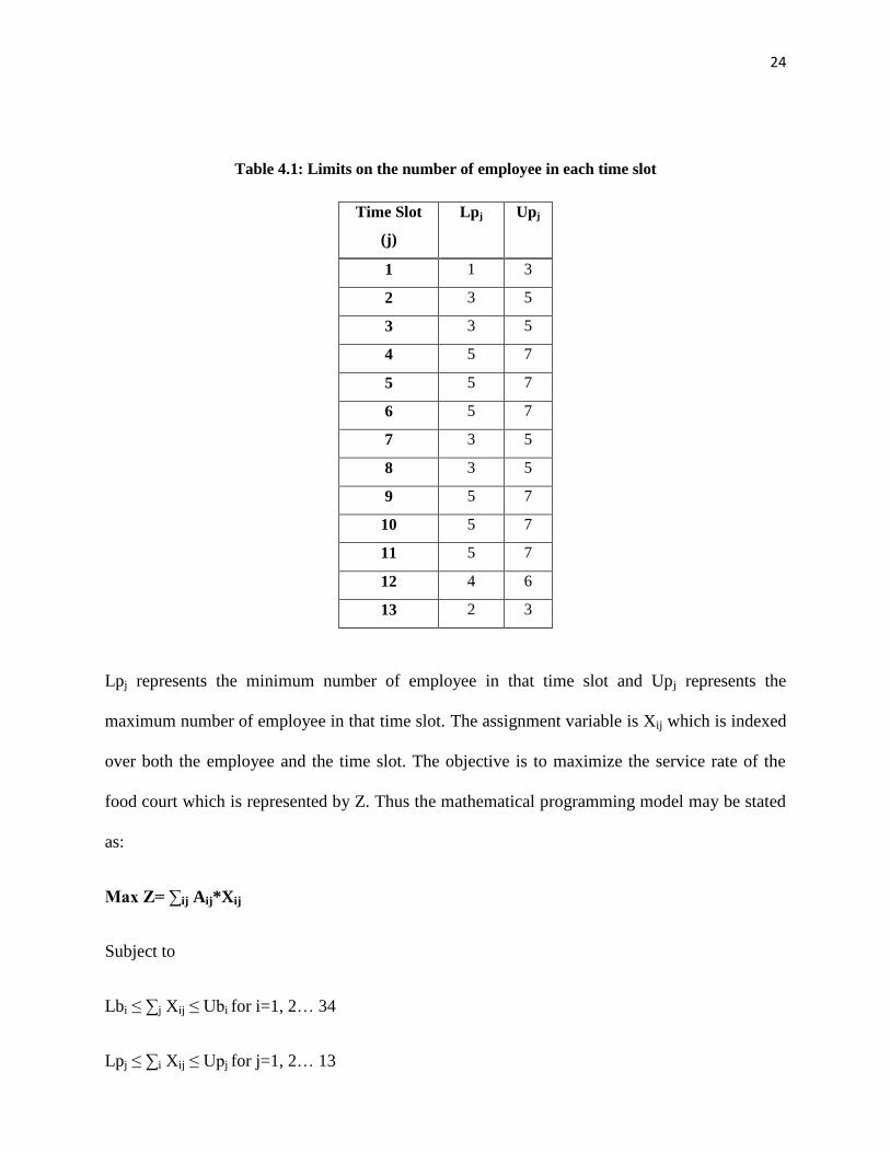
24
Table 4.1: Limits on the number of employee in each time slot
Time Slot
(j)
Lpj Upj
1 1 3
2 3 5
3 3 5
4 5 7
5 5 7
6 5 7
7 3 5
8 3 5
9 5 7
10 5 7
11 5 7
12 4 6
13 2 3
Lpj represents the minimum number of employee in that time slot and Upj represents the
maximum number of employee in that time slot. The assignment variable is Xij which is indexed
over both the employee and the time slot. The objective is to maximize the service rate of the
food court which is represented by Z. Thus the mathematical programming model may be stated
as:
Max Z= ∑ij Aij*Xij
Subject to
Lbi ≤ ∑j Xij ≤ Ubi for i=1, 2… 34
Lpj ≤ ∑i Xij ≤ Upj for j=1, 2… 13
25
Xij = (0, 1) binary for all i and j.
Detailed model can be found in Appendix C.
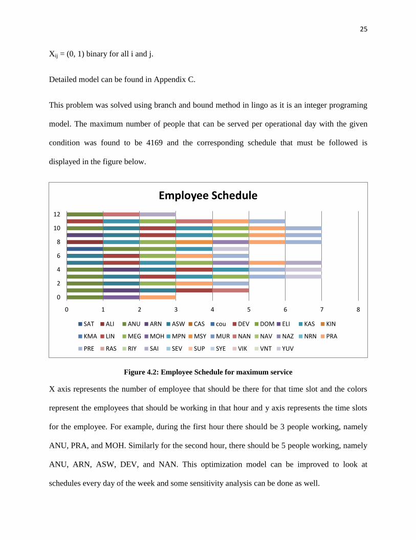
This problem was solved using branch and bound method in lingo as it is an integer programing
model. The maximum number of people that can be served per operational day with the given
condition was found to be 4169 and the corresponding schedule that must be followed is
displayed in the figure below.
Figure 4.2: Employee Schedule for maximum service
X axis represents the number of employee that should be there for that time slot and the colors
represent the employees that should be working in that hour and y axis represents the time slots
for the employee. For example, during the first hour there should be 3 people working, namely
ANU, PRA, and MOH. Similarly for the second hour, there should be 5 people working, namely
ANU, ARN, ASW, DEV, and NAN. This optimization model can be improved to look at
schedules every day of the week and some sensitivity analysis can be done as well.
0 1 2 3 4 5 6 7 8
0
2
4
6
8
10
12
Employee Schedule
SAT ALI ANU ARN ASW CAS cou DEV DOM ELI KAS KIN
KMA LIN MEG MOH MPN MSY MUR NAN NAV NAZ NRN PRA
PRE RAS RIY SAI SEV SUP SYE VIK VNT YUV
26
4.2 Restaurant Ranking
There are 20 restaurants in the food court and each has its own set of customers. Thus the sales
of each restaurant are completely dependent on the customer and the quality of food.
Unfortunately there is no data to support the quality of food, but an indirect factor might be the
number of people revisiting the restaurant. This is a valid assumption as, if the food is not good
then the customer will not be visiting the restaurant again (or the probability of revisit is very
low). Thus to see how each of the restaurants compete with other, all the restaurants are ranked
based on 3 factors.
1. Net sales per day, which is one of the basic criteria for ranking as it paints the picture of
how the restaurant is doing in general. If the sales is low then there are problems with the
restaurant and they need to be fixed quickly, these can be that menu items are not liked
by the customers, items are pricy, service rate is not up to standard, etc. and if the sales is
high then they are doing all of these things better, thus they can be an inspiration to
others.
2. Footfall, this tells the number of people purchasing some item from the restaurant per
day. This is also a simple but powerful way to see the performance of the restaurants. For
example the restaurant that has high footfall might indicate that the food is affordable,
items are preferred by the customer, and they are being served quickly. Thus it is
expected that net sales and footfall might have a similar pattern as if the number of
people increase then the sales increase as well.
3. Revisits, this will be an indirect way to check the quality of food. This statistic is a little
harder to calculate but it is comprehensive as it not only talks about the quality of food
but also all the above factors in footfall and net sales. A possible exception to this might

27
be restaurants that are really pricy and as a result even though the revisits are small the
quality of food might still be good. Thus it not an absolute factor to determine quality but
an approximate one.
Individual analysis for each of these components is documented below and the results for each
are discussed along with it as well.
4.2.1 Average Sales per Day
Average sales per day is the sales for the restaurant on any given day, this value is different for
each day and there are a number of factors affecting this, for the purpose of this thesis we are not
considering weighted sums or any other method. We calculate the net sales as the sum of all the
sales for that day. Then it is averaged over the days the sales happened.
Average sales per day = ∑
St = Net Sales for day t
N = Number of days
The graph below shows the net sales for each of the 20 restaurants. Restaurant 3, 7 and 20 show
sales in excess of Rs.30,000 which tells they make the maximum sales. Thus they have really
good performance, and some of the other restaurants are not too far behind which would imply if
they do some promotion then they can catch up with these leaders. But the sad part is that some
of the restaurants barely make an average sale of Rs. 10,000 which would imply there is
considerable catching up to do, and may be new items in the menu can do the trick.

28
Figure 4.3: Net Sales per day for all the twenty restaurants.
4.2.2 Footfall
Footfall is the number of unique visitors the restaurant has each day. This is calculated by
counting all the people served in the restaurant and then averaging out over the days. It is critical
as even though the sales is high if the number of customer served is low that means the price of
the items is relatively higher, which may imply that in the future this sales may not be consistent.
Thus there is scope for improvement.
Footfall = Count of customers
Number of days
It was hypothesized that this will be similar to the net sales, but there are some drastic
differences, which are clearly explained in the graph below. From the graph we can see that
restaurant 3 has way more customers than the remaining but still the sales are just on par with the
other restaurants, namely 20 and 7. This may be due to the fact that most of the items are
affordable. Another interesting fact is that the next sets of restaurants have about the same
number of customers but the sale is really varied, which would imply that some places are really
0
5000
10000
15000
20000
25000
30000
35000
40000
1 2 3 4 5 6 7 8 9 10 11 12 13 14 15 16 17 18 19 20
Net
Sa
les
in R
s.
Restaurants

29
pricy and some of them are really cheap. It may help to notice that even if the prices of some of
the cheap items are increased the demand might not be affected by much as there is a lot of
elasticity in the price.
Figure 4.4: Footfall for all the twenty restaurants
4.2.3 Revisits
Revisits are the number of people who not only come to that restaurants but do so repeatedly. It
calculated similar to Footfall but there is an inherent condition that they have been to that
restaurant at least once before. This is calculated by counting the customers and averaging them
over the days. This is an indirect measure of quality of food, because of the assumption that if the
food is not good then the customer will not come to restaurant again.
Revisits = Count of customers revisiting
Number of days
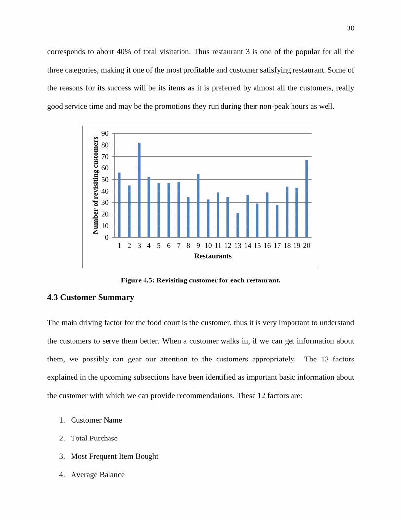
Surprisingly the figure below looks similar to Footfall for all the restaurants, which is acceptable
as revisits are a subset of Footfall. It is clear that restaurant 3 has the best quality food as out of
the 200 customers visiting the restaurant a day, about 80 of them are repeat customers, which
0
50
100
150
200
250
1 2 3 4 5 6 7 8 9 10 11 12 13 14 15 16 17 18 19 20
Fo
otf
all
Restaurant
30
corresponds to about 40% of total visitation. Thus restaurant 3 is one of the popular for all the
three categories, making it one of the most profitable and customer satisfying restaurant. Some of
the reasons for its success will be its items as it is preferred by almost all the customers, really
good service time and may be the promotions they run during their non-peak hours as well.
Figure 4.5: Revisiting customer for each restaurant.
4.3 Customer Summary
The main driving factor for the food court is the customer, thus it is very important to understand
the customers to serve them better. When a customer walks in, if we can get information about
them, we possibly can gear our attention to the customers appropriately. The 12 factors
explained in the upcoming subsections have been identified as important basic information about
the customer with which we can provide recommendations. These 12 factors are:
1. Customer Name
2. Total Purchase
3. Most Frequent Item Bought
4. Average Balance
0
10
20
30
40
50
60
70
80
90
1 2 3 4 5 6 7 8 9 10 11 12 13 14 15 16 17 18 19 20
Nu
mb
er o
f re
vis
itin
g c
ust
om
ers
Restaurants

31
5. Current Balance
6. Average Refill
7. Number of Visits
8. Average Discount Earned
9. Most Recent Restaurant Visited
10. Last Purchase Item
11. Most Visited Restaurant(s)
12. Net Purchase by Restaurant
For example one of the factors is the last restaurant visited, this can be used to give the customer
walking in a promotion that restaurant is running. Another example might be to use the last item
bought, to suggest other restaurants that carry the same item or a promotion for an accompanying
item. These are excellent ways to market the restaurant to customers as soon as they walk in.
The customer upon entry to the food court swipes his/her card at the registry. Each card has a
unique id. This can be used to filter all the data collected to provide some basic information
about the customer. One of the main problems customers face is that they need to walk to a cash
register every time they need to refill a card, and they are unsure on how much to refill for, so we
can recommend an average amount they have been spending in the food court every time they
visit in the past or if it is a first time user then use an average figure obtained from the past over
all customers.
For this analysis, an ideal customer, a customer who has been a regular visitor to the food court
and has purchased items from multiple restaurants, was chosen to explain all the basic
information as clearly as possible, thus these are not results of an average, but rather of an ideal
customer thus the numbers might be skewed from the average and also for all the customers all

32
these information may not be available. In the case where numerical values are missing, it is
replaced with the average value of all the customers. But if character values are missing, it shall
remain empty until the customer provides the information to fill it, like the customer name. For
this example, the customer is called John and his card was issued six months ago and all the
information is based on the six months of data collected on John by the card he uses during each
visit.
Customer summary is a one shot view of few of the basic information which consists of the
following:
4.3.1 Customer Name
Customer name is the name with which the customer prefers to be called. Even though the
customer can uniquely be identified by the customer id, the name makes it a bit more personal
thus enabling in better personalization. Along with name some more information like their phone
number and address can come in handy to do some more advanced analysis and marketing. In
about 80% of cases this field is empty, most probably because of privacy issues. This is not a
calculated field but it is entered manually by the creator or user. To protect the privacy of the
customer the actual name of the customer is replaced by a hypothetical one.
We consider a hypothetical ideal customer name, John.
4.3.2 Total Purchase
Total purchase is the sum of all the purchases John has done in this food court since this card
was issued to him 6 months ago. This includes purchases from all the restaurants and even all the
water bottles he purchased. Unfortunately if he has got a subsequent card then those transactions
are not added or tracked by this card. This is calculated by adding all the net amounts for every

33
item he has paid for with this card. This is obtained from the database by creating a filter for
John’s customer id.
Total Purchase by John = Rs. 6900
4.3.3 Most Frequent Items Bought
Most frequent item bought is the most common item bought by the customer apart from the most
frequently bought item in general namely, water bottle. As John is a repeat customer he
frequently buys the same items. He rarely ventures out to try new items. Thus he could be a
target for direct marketing. He has bought same few items seven times in the last six months and
at regular intervals. The actual item information is hidden for privacy purposes. Thus only the
item number is revealed. This information can be used to promote the same item but during
another visit. That is a coupon like 5% off on next purchase of that item. Promoting other
products to people of this category may not be relevant as they are not susceptible to change. The
frequently purchased item is derived from the database by counting the number of times a
customer buys every item and sorting it.
For John the 3 most frequently bought items are item numbers 97, 2093, and 2088.
4.3.4 Average Balance
Every time a customer refills a card the balance of the card changes, sometimes they refill when
the card balance is zero, sometimes when they come to the food court and in a few rare instances
they refill every time their balance reaches a threshold. In general, an ideal customer fills in the
balance when a threshold is reached. Average balance is calculated by adding all the elements in
the balance column which is recorded after every refill found in the card fill table and averaging
out by the number of time the customer refills the card. This is important to track because it

34
helps us identify what kind of customer he/she is. The most important take away is that people
who refill the card when it is completely empty should be moved to one of the other two
categories. The figure below shows the change in balance with every refill the customer places.
The average for these values is the Average Balance.
Average Balance of John = Rs. 430
Figure 4.6: Balance after each refill.
4.3.5 Current Balance
Every time a customer purchases an item the balance in the card is reduced and once all the
money in the card is used the customer will visit the cash register to refill it. To have excellent
customer satisfaction we should avoid customers from frequently visiting the cash register. To
enable this we can use the current balance which is the balance in the card at any point, and the
average balance to recommend how much they should refill so that they need not come back to
the cash registry soon. Current balance is calculated by taking the difference between all the
money added to the card and the total purchase till date.
Current Balance of John = Rs. 420
0
100
200
300
400
500
600
700
800
1 3 5 7 9 11 13 15 17 19 21 23 25
Am
ou
nt
in R
s.
Visits
balance

35
4.3.6 Average Refill Amount
Every time a customer refills the card it is recorded in the database as a separate transaction. This
helps in understanding the purchasing pattern of the customer and also to use their associated
demographic information. A member from a high income group will recharge for higher amount
compared to an individual from mid or low income group. Thus it is an effective tool to group
and classify them. Also tracking the refills helps us understand how frequently the customer runs
out of money which may be used in the future to start recommending when to do a refill and also
an amount to refill. The average refill amount is calculated by summing all the refill amounts and
dividing by the number of times refilled. The figure below shows the pattern of refill from this
customer over every refill visit.
Average Refill Amount of John = Rs. 265.
Figure 4.7: Refill Amount during each refill visit
This also shows that John is not from a high income group or single so that he does not need
much to be retained in the card.
0
100
200
300
400
500
600
1 3 5 7 9 11 13 15 17 19 21 23 25
Am
ou
nt
in R
s.
Visits
amount
36
4.3.7 Number of Visits
Every visit of a customer to the food court results in a transaction. Customers refill an existing
card, or get a new card, or if they have enough balance they directly go and purchase food items.
Thus the customer’s presence can be tracked electronically. This information is powerful as we
can use it to predict his next visit to a certain degree of accuracy, but unfortunately this is not a
within the scope of this thesis and can be done in the future. Thus the number of visits is a count
of number of times specifically dates on which at least one transaction is being entered.
Number of Visits of John = 42 from the time the card was issued to him six months ago.
4.3.8 Average Discount Earned
Discounts and promotions are not popular yet in the Indian culture, the restaurant owners were
happy with their current sales, but it is changing now. The restaurant owners have figured out
that most of their sales occurs during certain periods of time like during the lunch hours from 12
noon to 3 pm and during dinner from 7pm to 10pm. Thus to increase sales in the time between
the peaks they have started to give happy hours discount. Unfortunately this ideal customer has
not made use of these discounts as he visits mostly in the evenings after 7 pm which tells he is a
working class male. Average discount is calculated by adding all the discounts received divided
by the number of times the discount was received. As john has never received any discount
before his average discount is Rs. 0. If there he had earned discounts then it will be tracked under
calcdiscount column in bill details file, for which an average will be calculated.

37
4.3.9 Most Recent Restaurant Visited
Most customers who visit food courts try out new cuisines every time they visit the food court.
But some have standards and will hardly deviate from that. By tracking the last visited restaurant
we can see the changes in the customers’ behavior. A person who has been trying new things
every time might be interested in knowing about new places or promotions or specials in a
previously visited restaurant. This could be a change in pattern for them and attract many more
visits from them. If the person does not want to change has tried new restaurant then more new
restaurants can be recommended. Thus it is a critical part of the customer summary to understand
the customer better. The most recent restaurant visited is found by filtering the debit transactions
file for John and sorting by the date to find the last transaction he made. The restaurant where he
made the transaction is the most recent restaurant visited.
Most recent restaurant visited by John = Restaurant 3
4.3.10 Last Purchased Item
Similar to restaurants the items that people buy can also be coheres to change. For example, if a
person has been buying say a burger for last 3 times may be a coupon for a sub might change his
decision to get a sub instead of a burger again. Or else on the contrary if they have been buying
the same item repeatedly then you can encourage more sales from them in the future with
coupons and promotions. The last purchased item is selected from list of items the customer
bought in the last transaction.
Last Purchased Item by John = 2088 (Item Number)

38
4.3.11 Most Visited Restaurant(s)
Almost all customers have a favorite restaurant, the place from where they get their comfort
food. These customers are likely to visit this restaurant at least one a month and it is the food
court management’s duty to make sure this restaurant is available for them in this food court, so
that they can get regular customers throughout the year. Tracking this information can help in
effective marketing of the restaurant. Most visited restaurant is determined by counting the
number of visits the customer makes to each of the restaurants and flagging the highest one.
Most Visited Restaurant = Restaurant 8 (12 times) for the six months John has had the card.
4.3.12 Net Purchase by Restaurant
A very critical factor that needs to be tracked is where the customer spends most of his money,
knowing this can give us valuable insights into shaping the future of the food court. For example
if we know that a customer purchases most of his/her food from a restaurant we can start to
consolidate these into clusters and use this information to attract newer similar people and also
newer similar restaurants. If a restaurant is not doing well then they can be replaced with newer
and more preferred restaurants which can be determined by this data. The table below shows the
expenditure of John over all the restaurants he visited. It is notable that he has spent about 70%
of his money in his favorite restaurants. This is calculated by adding all the purchases and
grouping it by the restaurants.

39
Table 4.2: Amount spent in each restaurant
POScode Net Purchase (Rs.)
2 1748
3 316
4 791
7 1113
8 1258
10 881
11 326
12 124
17 103
18 259
4.4 Association Rule Mining
Association rules are implications which relate two or more items in a transaction. A simple
example of association is A => B which means presence of item A implies that item B is also
present. There are two factors that need to be satisfied to validate the claim. The first factor is
confidence; this is the probability with which this association is true. Second one is support; this
is the probability with which this association occurs in the complete dataset. The formula to
calculate the factors are below:
1. Confidence – P (B/A) where P is probability and B/A is B given A is true. Thus it is the
probability that B is true given that A is true.
2. Support – P ((A U B)/S), where S is the universal set. Thus it is the probability of A union
B occurring in the universal set or the complete dataset.
Both confidence and support are user defined factors and it is selected based on the dataset and
the accuracy with which you want to predict the association [Agrawal, 1993].
A food court transaction consists of all the items a customer buys in one bill. Thus we can
predict associations between menu items. As the dataset and the number of customers are large
40
and changing these associations can help in generalizing some of the common characteristics of
new customers coming to the food court. For example one of the association found is that people
who buy menu item 2088 also buy menu item 97, thus a new customer who buys 2088 will most
probably buy 97 as well, which is a really good insight into a customer on whom we have no
information.
Association rules can be calculated by many different ways, namely Apriori algorithm, Eclat
algorithm, FP-growth algorithm, etc. For this thesis we select Apriori algorithm, as a
representative. The main reason is the simplicity and scalability of this algorithm. The results
from this may not be most accurate but it will give the reader an understanding of how the results
of association rule mining can be used in the context of a food court.
4.4.1 Apriori Algorithm
Apriori is an algorithm used to find associations in large transactional databases. It identifies
frequent item sets that satisfy the user defined support and then it is rerun by extending the
dataset to a larger one until the support is broken. When the cycle is broken, the previous set is
the largest possible set that has the minimum support from the database. Apriori uses breadth
first approach to completely exhaust all the large item sets that satisfy the support and that mean
all the subsets of this set also satisfy the support specified. After the support is satisfied, it will
check the confidence to make sure both the conditions are met by all the associations [Agrawal,
1994].
Apriori is not the fastest way to check for association but the bottom-up exploration makes sure
that the accuracy is very high. One of the main problems with this might be the time it takes to
find the associations, but it is thorough in its analysis, thus very useful in this case as the dataset
is not really huge and time taken is not significantly high. May be in the future we can compare

41
the results of Apriori algorithm with other competing algorithms like Eclat, FP growth, etc. to
see the short falls in detail. But for the purpose of this thesis these results will be sufficient to
derive useful conclusions.
To find the associations in this database, we used R’s package, Arules which has the Apriori
algorithm prefilled and with an input of a transaction table the results are relatively easy to
retrieve. The transaction table used for this computation is the bill details file where all the
transactions are uniquely identified by Bill Number and there are multiple items being bought in
one bill, represented by Menu Item Code. The results of this are displayed in the table below, due
to size constraints not all the association that satisfy the condition are displayed, but only fifteen
most relevant ones are displayed.
It is clear from the Table 4.3 that there are a number of single relationships and a few multiple
relationships that satisfies the support of 0.1 and confidence of 0.3. Single relationships refer to
rules that have one item in the left hand side and one item in the right hand side, whereas
multiple relationship refers to more than one item in the left hand side and one item in the right
hand side. As the data is really vast with a lot of transaction it is hard to have a high support or
confidence. The results show that there about 101 rules that satisfies the minimum support of 0.1
and minimum confidence of 0.3, but only the sample set of 15 rules are displayed in table 4.3,
the complete set of rules can be found in Appendix D. From the results it can be determined that
there is a clear association between items 2088 and 97. Thus we can make combo deals like both
these products together can be sold for a lower price, or we can use this formation to promote
another product that in not frequently bought to be sold to move inventory.
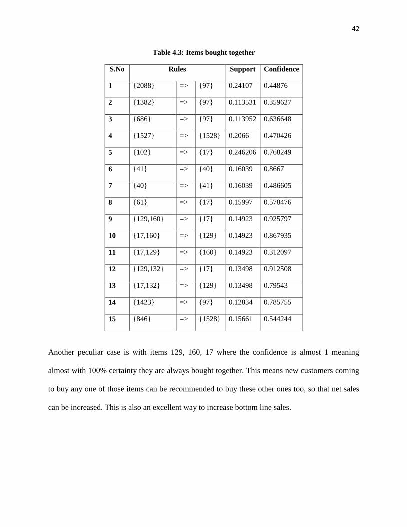
42
Table 4.3: Items bought together
S.No Rules Support Confidence
1 {2088} => {97} 0.24107 0.44876
2 {1382} => {97} 0.113531 0.359627
3 {686} => {97} 0.113952 0.636648
4 {1527} => {1528} 0.2066 0.470426
5 {102} => {17} 0.246206 0.768249
6 {41} => {40} 0.16039 0.8667
7 {40} => {41} 0.16039 0.486605
8 {61} => {17} 0.15997 0.578476
9 {129,160} => {17} 0.14923 0.925797
10 {17,160} => {129} 0.14923 0.867935
11 {17,129} => {160} 0.14923 0.312097
12 {129,132} => {17} 0.13498 0.912508
13 {17,132} => {129} 0.13498 0.79543
14 {1423} => {97} 0.12834 0.785755
15 {846} => {1528} 0.15661 0.544244
Another peculiar case is with items 129, 160, 17 where the confidence is almost 1 meaning
almost with 100% certainty they are always bought together. This means new customers coming
to buy any one of those items can be recommended to buy these other ones too, so that net sales
can be increased. This is also an excellent way to increase bottom line sales.

43
4.5 Clustering Analysis
In a food court where 100’s of customers are served every day, there are similarities between the
purchasing behaviors of different people. An excellent way to find out these groups is through
clustering analysis. Clustering analysis looks for similarities within the groups with an objective
of having similar things in a group and the items across different groups are dissimilar.
Depending on what the user wants to find, different types of clustering models can be used like,
hierarchical clustering based on distance connectivity, K-mean for centroid based instead of
actual data points, or density based models like DBSCAN, Optics, etc., [Castro, 2002]. For the
purpose of this thesis we look at k-mean clustering because of its usability with highly scattered
data and its ease of use for conducting analysis and experimentation. With k-mean clustering the
runtime of analysis was significantly less thus multiple runs were possible with different number
of clusters.
For k-means clustering the number of clusters k should be predetermined and as we do not know
how many clusters are there in this data we need to run multiple iterations to find out the optimal
number of clusters. Thus a shorter runtime is essential. In k-mean clustering we try to minimize
the within cluster sum of squares [Kanungo, 2002]. To begin we assume the number of clusters
to be 10 and run the analysis. Thus the data set is separated into 10 groups and the centroid for
each is calculated. Then it looks for other elements that is closer to this mean than others using
sum of squares. This happens for each observation and finally all the observations are grouped
into one of ten clusters. But it is impossible to say if ten is the number of clusters needed to
explain the data or not, thus multiple runs with different number of clusters needed to find the
best groups.

44
In this thesis clustering analysis was done on one full year’s data looking at the purchasing
behavior of each customer for every week in every restaurant. Number of optimal customers for
this dataset was seven. Each of the six clusters defines different kinds of customers that are
served in the food court. The figure 4.8 clearly shows the seven different clusters. First one is the
one time shoppers, people that come to food court only once or people who get a new card for
their every visit. They constitute for about 70% of the transactions in the food court. They are
represented with pink. The second group will be the long time regular customers who spend a lot
of money, the high rollers. They are represented in Red. The third group is people who come to
throw a party for friends mostly likely just once during the summer, the free spirits. They are
represented by navy blue. The fourth group is the friendly neighbors, people who are regular but
spend the same amount in multiple restaurants trying different restaurants every visit. They are
represented by yellow. The fifth group is the classics; they are the typical customers who visit
the food court for the same food every time. They are represented by black. The sixth group is
holiday shoppers; they are average consumers who visit only during the holiday season the
summer, festivals, public holidays etc. They are represented by green. The seventh group is set
of people that randomly come to food court and spend different amounts, the outliers. They are
represented by sky blue. These are seven very broad clusters of customers, each of which are
unique in their own way.
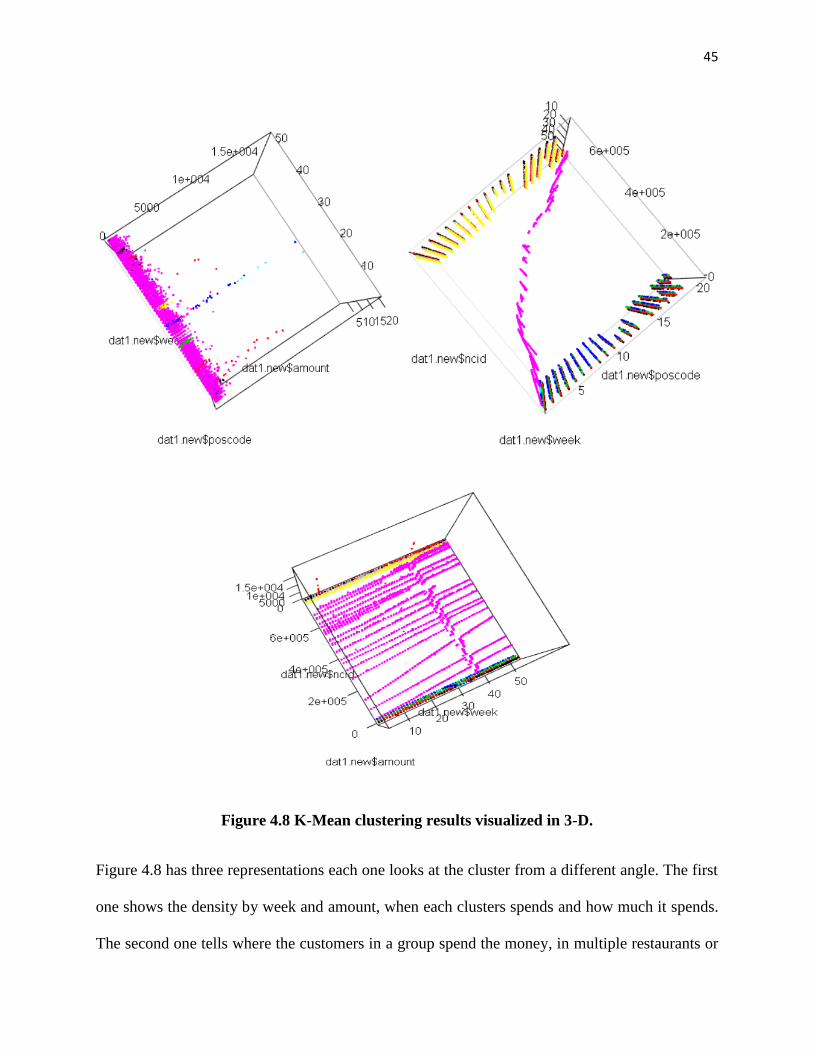
45
Figure 4.8 K-Mean clustering results visualized in 3-D.
Figure 4.8 has three representations each one looks at the cluster from a different angle. The first
one shows the density by week and amount, when each clusters spends and how much it spends.
The second one tells where the customers in a group spend the money, in multiple restaurants or

46
in the same restaurant. The third one shows the customer, week and amount to better explain
how the customer purchases change with time. In the third figure there is lot of gaps emphasizing
that not all customers visit the food court repeatedly and the cross lines tells they visit only once.
This clustering analysis has clearly segregated the customer into groups which can be used for
customer segmentation, direct marketing, promotional coupons, etc. As these groups are volatile
they can be moved from one to another by creative marketing. For example, if we send a coupon
like “Spend more than Rs.1000 to get a discount of 20%” to the friendly neighbor asking them to
spend more than their usual to get a discount they can be moved to high rollers soon as they
spend more on their every visit to get the discount. Another example might be coupons like “5%
off on your next purchase if you use the same card” for the one time shoppers are encouraged to
keep the same card for longer periods of time making them regulars. These are just a few
examples on how this information can be used. Inputting this as a dashboard component will
give an added advantage for the management to use with the customer summary to serve the
customers much more efficiently.

47
Chapter 5
Conclusions and Recommendations
The objective of the thesis is to provide some basic analytics to build a dashboard for the food
court management to understand what the current scenario of the food court is and provide
insights as to how to improve certain aspects such as: employee satisfaction, customer
satisfaction and restaurant satisfaction. Employee satisfaction can be achieved by making sure all
the employee are not over worked and they are given adequate breaks to keep them energized to
work to their maximum potential during their shifts and an optimal employee schedule has been
calculated to ensure that no employee works for more than 8 hours and there are breaks for every
employee during the day to refresh and recharge. This optimal employee schedule was
determined by using the each employee’s service rate during each hour of an average operational
day to optimize for maximum service of customers. According to the results during the first of
the day three people need to be working, namely ANU, PRA and MOH.
Customer satisfaction is the most critical one as customers are the driving factor for the food
court, thus making sure they do not waste time unnecessarily in queues, when they can avoid it.
This can be achieved by using the customer summary to recommend customers on how much to
refill the card or how much to purchase the card for, so that they need not come back to stand in
the refill queue again the same day. We can also use the customer summary information to
recommend items for them to try based on their previous purchases, or may recommend a
restaurant that may be running a promotion that they can make use of to save some money.
Using the customer summary we can also build a basic profile for the customers. For example
for the customer described in the analysis John, is a male, working in an office, belonging to the
mid-income group, who visits the food court at least once every week and spends 70% of the

48
money in the same three restaurants namely restaurants 2, 7 and 8. This creates a profile for the
customer which can be further developed using some more customer inputs in the future. The
clustering analysis can be used along with the customer summary to classify the customer into
one of seven clusters so that targeted marketing can be used to move the customers from one
group to another.
Restaurant satisfaction is also important as turnover of restaurants can be hard on loyal
customers, the brand image of the food court may be damaged, and it will be a challenge to get
new customers. By ranking the restaurants with their competition we can segregate the
restaurants as self-sufficient restaurants, and restaurants that need help in attracting more
customers. It is clear from the analysis that some restaurants are doing very well namely
restaurants 3, 7, 20 and some are struggling namely restaurants 4, 13,14, and 16. Thus it is up to
the management to help the underperforming restaurants increase their loyal customer base with
a lot of promotion and joint marketing with other restaurant in the food court. The restaurants
can also use the association rules to help with their marketing and promotions campaign.
Another usefulness of the association rule is for the restaurant to better forecast their sales for the
future, thus plan accordingly.
5.1 Recommendations
1. Currently all the employees are not being utilized properly and there is considerable
variation in their performance throughout the day which may be due to over working.
Thus implementing this new employee schedule will enable in increasing the productivity
of employee and also make sure that they do not work for more than 8 hours.
2. Customers wait in the queue for refills multiple times in a short period of time; this
implies that the customer is not clear on what he/she wants to buy and how much it is

49
going to cost him/her. It becomes the employees’ responsibility to use the customer
summary information to suggest items to the customer and also how much to refill for.
This will result in increased customer satisfaction.
3. Using the Association rules, a new marketing strategy can be implemented so that the
customers are better spread rather than purchasing from the same few restaurants
repeatedly. This information can also be used to generate coupons for accompanying
items to increase their sales as well.
4. The database has considerable redundant information which occupies unnecessary space
which can be avoided. This space can be used to collect more information about the
customers to help better understand them. For example, their names should be filled
100% of the time, along with name their phone number can be used to send promotions
and discount coupons, and also their address to help us with some clustering analysis of
purchasing by customers from different neighborhoods.
5. The management should encourage restaurants to be more adventurous in introducing
new and exclusive items during different periods to attract newer customers.
6. Restaurants should use all of their resources to make sure that the customers are served
promptly with great quality food, which will ensure the customers coming back for more
in the future.
7. A new method to collect customer feedback should be implemented as current level of
customer information may not be sufficient for details study of patterns and clusters.
8. Coupons should be distributed to customers based on their clusters to move them. This
can also be used to change the customer and encourage them for regular visits.
9. The clustering analysis can be used to segregate the new customers into one of these
groups and use this information to provide better customer service.
50
Chapter 6
Future Work
The scope of this thesis is very limited. In this thesis we introduced the use of analytics to food
court, which will help the management use some of the common information collected by the
database to improve the bottom line of the food court, and eventually the restaurants. The
purpose is to familiarize the management to dashboard and how and what kind of information
can be displayed in it. Moreover the database has some problems with redundant data which
increases noise when performing advanced analytics, thus the database should be redesigned to
avoid this in the future.
The dataset is vast and contains much more information than what has been used in this thesis.
As this thesis is a preliminary view of analytics in food court none of the advanced analytics
methods were tried and also in most of the analysis done here there are preliminary and alternate
methods can be tried. This data set can also be used to do some further analysis using some of
the following techniques:
1. Time series analysis: Every transaction in this food court has a timestamp, thus we can
track the actions of a customer right from when he enters to when he leaves the food
court. This kind of detailed study requires a lot of time and advanced knowledge on time
series. By building a time series we can find out customer purchasing patterns. This
information can be useful for the restaurants to strategize marketing campaigns around it.
Thus time series analysis is a separate path that can be studies with this kind of database.
2. Network clustering: The customer information is very limited in the current database,
thus is hard to construct network cluster around them. To do this analysis we need to

51
collect some more data from the customer. Each customer should give their name, phone
number and address. This information can then be used to map a network of all the
customers visiting the food court with their current addresses. With this we can make
clusters of customers belonging to certain groups and build classification models based
on that. This kind of advanced analytics can be used by both the food court management
as to how to increase the spread of the network and by the restaurants to understand what
kinds of people buy their kind of food.
3. Customer profiling: In the customer summary we were able to predict a few of the details
about the customer. But with more understanding of all the remaining information and
the new information like name, phone number and address we can build a more
comprehensive profile for a customer and use this information to predict the behavior of
new customers and their purchases. We can build classification of standard customers
based on their behavior and this can be used to sort the remaining. For example, there
might be a large portion of college students who visit the food court on Friday evening
before going to a movie, so we know they need something fast and may be a little bit
inexpensive, so we can create a classification for this and sort the new customer into this
if they follow the same criteria. This information can be further used for targeted
marketing as we known what they might be interested in.
4. Restaurant profiling: Similar to customers the restaurants have patterns too; we can track
their service time, number of transactions per hour, items sold during each hour of an
operational day, etc. This information can then be used to see what is being done by
restaurants with good metrics and develop blue prints for “good restaurants.” This

52
information can also be used find out bad restaurants that are damaging the food courts
reputation and replace them with newer restaurants that the customers like.
5. Predictive Forecasting: The sale of every item is tracked with time and date information.
Using this we can build a predictive model to see when the next purchase of the item is
going to occur and may be even predict which customer is going to purchase it. This can
then be extrapolated to create a forecasting model for the sales of all the items in a
restaurant. This method will have much more accuracy as we have predicated the next
purchase with all the historical sales information. This can even be extended to create an
inventory model for replenishment of raw materials to produce these food items.

53
REFERENCES
Fayyad, U. M., Piatetsky-Shapiro, G., Smyth, P., & Uthurusamy, R. (1996). Advances in
knowledge discovery and data mining.
Kohavi, R., Rothleder, N. J., & Simoudis, E. (2002). Emerging trends in business analytics.
Communications of the ACM, 45(8), 45-48.
Vitaly Friedman (2008) "Data Visualization and Infographics" in: Graphics, Monday
Inspiration, January 14th, 2008.
Agrawal, R., & Srikant, R. (1994, September). Fast algorithms for mining association rules.
In Proc. 20th int. conf. very large databases, VLDB (Vol. 1215, pp. 487-499).
Agrawal, R., Imieliński, T., & Swami, A. (1993, June). Mining association rules between sets
of items in large databases. In ACM SIGMOD Record (Vol. 22, No. 2, pp. 207-
216). ACM.
Brizek, M. G., & Khan, M. A. (2002). Ranking of US hospitality undergraduate programs:
2000–2001. Journal of Hospitality & Tourism Education, 14(2), 4-8.
Lin, W., Alvarez, S. A., & Ruiz, C. (2002). Efficient adaptive-support association rule
mining for recommender systems. Data mining and knowledge discovery, 6(1), 83-
105.
Love, R. R., & Hoey, J. M. (1990). Management science improves fast-food operations.
Interfaces, 20(2), 21-29.
Ma, B. L. W. H. Y. (1998). Integrating classification and association rule mining. In
Proceedings of the 4th.

54
Snyder, B., & Barzilay, R. (2007). Multiple Aspect Ranking Using the Good Grief
Algorithm. In HLT-NAACL (pp. 300-307).
Min, H., & Min, H. (2011). Benchmarking the service quality of fast-food restaurant
franchises in the USA: a longitudinal study. Benchmarking: An International
Journal, 18(2), 282-300.
Hipp, J., Güntzer, U., & Nakhaeizadeh, G. (2000). Algorithms for association rule mining—a
general survey and comparison. ACM SIGKDD Explorations Newsletter, 2(1), 58-
64.
Shaw, M. J., Subramaniam, C., Tan, G. W., & Welge, M. E. (2001). Knowledge management
and data mining for marketing. Decision support systems, 31(1), 127-137.
Wang, L., Lou, T., Tang, J., & Hopcroft, J. E. (2011, December). Detecting community
kernels in large social networks. In Data Mining (ICDM), 2011 IEEE 11th
International Conference on (pp. 784-793). IEEE.
Liu, L. M., Bhattacharyya, S., Sclove, S. L., Chen, R., & Lattyak, W. J. (2001). Data mining
on time series: an illustration using fast-food restaurant franchise data.
Computational Statistics & Data Analysis, 37(4), 455-476.
Kim, Y. S., Moreo, P. J., & Yeh, R. J. (2005). Customers' satisfaction factors regarding
university food court service. Journal of Foodservice Business Research, 7(4), 97-
110.
K. Crammer, Y. Singer. (2001). Pranking with ranking. In NIPS, 641-647.
55
R. Higashinaka, R. Prasad, M. Walker. (2006). Learning to generate naturalistic utterances
using reviews in spoken dialogue systems. In Proceedings of COL-ING/ACL, 265-
272.
Estivill-Castro, V. (2002). Why so many clustering algorithms: a position paper. ACM
SIGKDD Explorations Newsletter, 4(1), 65-75.
Kanungo, T., Mount, D. M., Netanyahu, N. S., Piatko, C. D., Silverman, R., & Wu, A. Y.
(2002). An efficient k-means clustering algorithm: Analysis and
implementation. Pattern Analysis and Machine Intelligence, IEEE Transactions
on, 24(7),881-892.

56
APPENDICES
Appendix A: Current Database Design
Table 1: Debit transactions
Heading Description
Debitcode Classification Between Cash And Credit
Cardno Unique Identifier Of The Customer
Cardcode Unique Identifier Of The Card
Poscode Restaurant Classification
Tranno Restaurant Transaction Number
Amount Price Of Purchase
Balance Remaining Balance
Membname Name Of Card Holder (Incomplete)
Ctranno Management Transaction Number
Sopr Abbreviation Of Employee
Auddt Date Of Transaction
Trandtm Time Of Transaction

57
Table 2: Card Fill
Heading Description
Redeem Refund Classification
Debitcode Cash Or Credit
Cardno Unique Identifier Of The Customer
Cardcode Unique Identifier Of The Card
Paymode Mode Of Payment
Cash Cash Paid
Credit Credit Paid
Ctranno Management Transaction Number
Rtranno Backup Transaction Number
Issudtm Card Issue Time
Issudt Card Issue Date
Redmdtm Card Redeem Time
Redmdt Card Redeem Date
Exprdt Card Expiration Date
Amount Net Value Of The Card
Amount1 Top Up To The Card
Balance Current Balance
Refund Amount Refunded
Membname Name Of Customer
Redmopr Redeem Employee
Sopr Issuing Employee
Auddt Transaction Date
Bfbalance Balance Brought Forward
Unredeemable Amount Not Refundable
Balance1 Net Balance On The Card
Topupno Number Of Top-ups
Mobileno Mobile Number Of Customer

58
Table 3: Bill Details
Heading Description
ID Unique Identifier
Billno Restaurant Bill No
Serialno Line Items
Menuitemcode Code Of Purchased Item
Incomeheadcode Mode Of Payment
Quantity Quantity Purchased
Menuheadcode Category Of Item
Menugroupcode Group Of Item
Menusubgroupcode Subgroup Of Item
Rate Unit Price
Originalrate Actual Price
Backwardrate Previous Price
Cost Cost Of Production
Discount Discount Offered
Discountindicator Reason For Discount
Discounttype Category Of Discount
Calcdiscount Amount Discounted
Netamount Total Purchasing Price
Createddate Time Of Creation
Ratecode Unit Price Reference
Kotdate Date Of Purchase
Kottime Time Of Purchase
Itemtotaltax Total Tax On The Item
Table 4: Daily Sales Close
Heading Description
Date Close Date
Cashiercd Employee Id
Cash Total Cash Collected
Credit Total Credit Collected
Refund Amount Refunded
Balance Balance Not Accounted For
Withdraw Total Money In The Bank
Debcredit Cash To Be Paid To The Restaurant
Sopr Employee Id
Auddt Close Time

59
Table 5: Reissued Cards
Heading Description
Trandtm Transaction Time
Debitcode Mode Of Payment
Cardno Unique Identifier Of The Customer
Oldctranno Old Management Transaction Number
Newctranno New Management Transaction Number
Balance Previous Balance
Membname Members Name
Sopr Issuing Employee Id
Auddt Issue Date
Table 6: Line Void
Heading Description
Deletedid Unique Identifier
Linevoidid Deleted Item Id
Kotno Transaction Id
Kotdatetime Time Of Cancelation
Menuitemcode Item Canceled
Quantity Quantity Canceled
Createddate Cancelation Date
Amount Total Amount Refunded
Table 7: Kot Total Tax
Heading Description
ID Unique Identifier
Kotno Transaction Id
Kotdatetime Time Of Purchase
Taxcode Tax Classification
Taxamt Total Tax
Taxableamt Total Amount Taxed
Createddate Date Of Purchase

60
Table 8: Kot Item Tax
Heading Description
ID Unique Identifier
Kotno Transaction Id
Kotdatetime Time Of Purchase
Serialno Line Item Number
Menuitemcode Code Of Purchased Item
Menuheadcode Category Of Item
Taxcode Tax Classification
Taxamount Total Tax
Taxableamount Total Amount Taxed
Createddate Date Of Purchase
Table 9: Kot Head
Heading Description
Kotno Transaction Id
Kotdatetime Time Of Purchase
Tableroomcode Unique Identifier
Amount Net Purchase Amount
Taxamount Total Tax Paid
Createddate Date Of Purchase
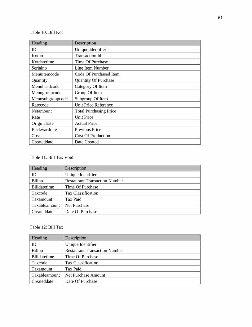
61
Table 10: Bill Kot
Heading Description
ID Unique Identifier
Kotno Transaction Id
Kotdatetime Time Of Purchase
Serialno Line Item Number
Menuitemcode Code Of Purchased Item
Quantity Quantity Of Purchase
Menuheadcode Category Of Item
Menugroupcode Group Of Item
Menusubgroupcode Subgroup Of Item
Ratecode Unit Price Reference
Netamount Total Purchasing Price
Rate Unit Price
Originalrate Actual Price
Backwardrate Previous Price
Cost Cost Of Production
Createddate Date Created
Table 11: Bill Tax Void
Heading Description
ID Unique Identifier
Billno Restaurant Transaction Number
Billdatetime Time Of Purchase
Taxcode Tax Classification
Taxamount Tax Paid
Taxableamount Net Purchase
Createddate Date Of Purchase
Table 12: Bill Tax
Heading Description
ID Unique Identifier
Billno Restaurant Transaction Number
Billdatetime Time Of Purchase
Taxcode Tax Classification
Taxamount Tax Paid
Taxableamount Net Purchase Amount
Createddate Date Of Purchase

62
Table 13: Bill Print
Heading Description
ID Unique Identifier
Billno Restaurant Transaction Number
Printtime Time Of Purchase
Printdate Date Of Purchase
Bill Amount Actual Amount Paid Including Tax
Table 14: Kot
Heading Description
ID Unique Identifier
Billno Restaurant Transaction Number
Billmadedatetime Time Of Purchase
Billvoiddatetime Date Of Purchase
Kotno Transaction Id
Table 15: Item Tax Void
Heading Description
ID Unique Identifier
Billno Restaurant Transaction Number
Billdatetime Time Of Purchase
Serialno Line Item Number
Menuitemcode Code Of Purchased Item
Menuheadcode Category Of Item
Taxcode Tax Classification
Taxamount Tax Paid
Taxableamount Net Purchase Amount
Createddate Date Of Purchase

63
Table 16: Item Tax
Heading Description
ID Unique Identifier
Billno Restaurant Transaction Number
Billdatetime Time Of Purchase
Serialno Line Item Number
Menuitemcode Code Of Purchased Item
Menuheadcode Category Of Item
Taxcode Tax Classification
Taxamount Tax Paid
Taxableamount Net Purchase Amount
Createddate Date Of Purchase
Table 17: Bill Head Void
Heading Description
ID Unique Identifier
Voidreason Void Reason Classification
Voiddate Date Of Purchase
Voidtime Time Of Purchase
Billno Restaurant Transaction Number
Totaltax Tax Paid
Roundoffamount Approximation To Nearest 10
Billamount Actual Amount Paid Including Tax
Table 18: Bill Head
Heading Description
ID Unique Identifier
Billno Restaurant Transaction Number
Billmadedate Date Of Purchase
Billmadetime Time Of Purchase
Totaltax Tax Paid
Totaldiscount Discount Offered
Roundoffamount Approximation To Nearest 10
Billamount Actual Amount Paid Including Tax
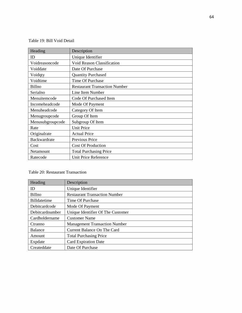
64
Table 19: Bill Void Detail
Heading Description
ID Unique Identifier
Voidreasoncode Void Reason Classification
Voiddate Date Of Purchase
Voidqty Quantity Purchased
Voidtime Time Of Purchase
Billno Restaurant Transaction Number
Serialno Line Item Number
Menuitemcode Code Of Purchased Item
Incomeheadcode Mode Of Payment
Menuheadcode Category Of Item
Menugroupcode Group Of Item
Menusubgroupcode Subgroup Of Item
Rate Unit Price
Originalrate Actual Price
Backwardrate Previous Price
Cost Cost Of Production
Netamount Total Purchasing Price
Ratecode Unit Price Reference
Table 20: Restaurant Transaction
Heading Description
ID Unique Identifier
Billno Restaurant Transaction Number
Billdatetime Time Of Purchase
Debitcardcode Mode Of Payment
Debitcardnumber Unique Identifier Of The Customer
Cardholdername Customer Name
Ctranno Management Transaction Number
Balance Current Balance On The Card
Amount Total Purchasing Price
Expdate Card Expiration Date
Createddate Date Of Purchase

65
Table 21: Debit Payment
Heading Description
Amount Price Of Purchase
Name Customer Name
Expdate Card Expiration Date
Chqdate Date Of Purchase
Ctranno Management Transaction Number
Auddt Time Of Purchase
Topupno Number Of Top Ups

66
Appendix B: Proposed Database Design
Table 1: Debit transactions
Heading Description
Debitcode Classification Between Cash And Credit
Cardno Unique Identifier Of The Customer
Poscode Restaurant Classification
Tranno Restaurant Transaction Number
Amount Price Of Purchase
Balance Remaining Balance
Membname Name Of Card Holder (Incomplete)
Ctranno Management Transaction Number
Sopr Abbreviation Of Employee
Auddt Date Of Transaction
Trandtm Time Of Transaction
Table 2: Card Fill
Heading Description
Redeem Refund Classification
Debitcode Cash Or Credit
Cardno Unique Identifier Of The Customer
Cash Cash Paid
Credit Credit Paid
Ctranno Management Transaction Number
Rtranno Backup Transaction Number
Issudtm Card Issue Time
Issudt Card Issue Date
Redmdtm Card Redeem Time
Redmdt Card Redeem Date
Exprdt Card Expiration Date
Amount Net Value Of The Card
Amount1 Top Up To The Card
Balance Current Balance
Refund Amount Refunded
Membname Name Of Customer
Redmopr Redeem Employee
Sopr Issuing Employee
Topupno Number Of Top-ups
Mobileno Mobile Number Of Customer

67
Table 3: Bill Details
Heading Description
ID Unique Identifier
Billno Restaurant Bill No
Serialno Line Items
Menuitemcode Code Of Purchased Item
Incomeheadcode Mode Of Payment
Quantity Quantity Purchased
Menuheadcode Category Of Item
Menugroupcode Group Of Item
Menusubgroupcode Subgroup Of Item
Rate Unit Price
Cost Cost Of Production
Discount Discount Offered
Discountindicator Reason For Discount
Discounttype Category Of Discount
Calcdiscount Amount Discounted
Netamount Total Purchasing Price
Ratecode Unit Price Reference
Kotdate Date Of Purchase
Kottime Time Of Purchase
Itemtotaltax Total Tax On The Item
Table 4: Daily Sales Close
Heading Description
Date Close Date
Cashiercd Employee Id
Cash Total Cash Collected
Credit Total Credit Collected
Refund Amount Refunded
Balance Balance Not Accounted For
Withdraw Total Money In The Bank
Auddt Close Time

68
Table 5: Bill Void Detail
Heading Description
ID Unique Identifier
Voidreasoncode Void Reason Classification
Voiddate Date Of Purchase
Voidqty Quantity Purchased
Voidtime Time Of Purchase
Billno Restaurant Transaction Number
Serialno Line Item Number
Menuitemcode Code Of Purchased Item
Incomeheadcode Mode Of Payment
Menuheadcode Category Of Item
Menugroupcode Group Of Item
Menusubgroupcode Subgroup Of Item
Rate Unit Price
Cost Cost Of Production
Taxamount Tax Paid
Netamount Total Purchasing Price
Ratecode Unit Price Reference
Table 6: Restaurant Transaction
Heading Description
ID Unique Identifier
Billno Restaurant Transaction Number
Billdatetime Time Of Purchase
Debitcardcode Mode Of Payment
Debitcardnumber Unique Identifier Of The Customer
Cardholdername Customer Name
Ctranno Management Transaction Number
Balance Current Balance On The Card
Amount Total Purchasing Price
Totaltax Tax Paid
Totaldiscount Discount Offered
Roundoffamount Approximation To Nearest 10
Expdate Card Expiration Date
Createddate Date Of Purchase

69
Appendix C: Optimization Model
MODEL:
[_1] MAX= 23 * X_1_3 + 15 * X_1_4 + 22 * X_1_5 + 7 * X_1_6 + 19 * X_1_8
+ 6 * X_1_9 + 5 * X_1_11 + 2 * X_1_12 + X_1_13 + 9 * X_1_14 + 9 * X_1_15
+ 19 * X_1_16 + 5 * X_1_18 + 14 * X_1_20 + X_1_22 + 12 * X_1_23 + 30 *
X_1_24 + 18 * X_1_25 + 6 * X_1_28 + X_1_29 + 2 * X_1_30 + 7 * X_1_32 + 9
* X_1_33 + 15 * X_1_34 + 2 * X_2_1 + 6 * X_2_2 + 61 * X_2_3 + 34 * X_2_4
+ 52 * X_2_5 + 4 * X_2_6 + 7 * X_2_7 + 39 * X_2_8 + 12 * X_2_9 + 2 *
X_2_10 + 17 * X_2_11 + 7 * X_2_12 + X_2_13 + 20 * X_2_14 + 56 * X_2_15 +
8 * X_2_16 + 14 * X_2_18 + 34 * X_2_20 + 9 * X_2_22 + 23 * X_2_23 + 47 *
X_2_24 + 48 * X_2_25 + 3 * X_2_26 + 6 * X_2_27 + 18 * X_2_28 + 6 *
X_2_29 + X_2_31 + 22 * X_2_32 + 17 * X_2_33 + 32 * X_2_34 + 11 * X_3_1 +
27 * X_3_2 + 87 * X_3_3 + 37 * X_3_4 + 69 * X_3_5 + 13 * X_3_6 + 30 *
X_3_7 + 61 * X_3_8 + 29 * X_3_9 + 42 * X_3_11 + 15 * X_3_12 + 2 * X_3_13
+ 16 * X_3_14 + 89 * X_3_15 + 12 * X_3_16 + 16 * X_3_18 + 30 * X_3_20 +
24 * X_3_22 + 27 * X_3_23 + 74 * X_3_24 + 75 * X_3_25 + 10 * X_3_26 + 9
* X_3_27 + 34 * X_3_28 + 16 * X_3_29 + 11 * X_3_31 + 20 * X_3_32 + 15 *
X_3_33 + 56 * X_3_34 + 9 * X_4_1 + 25 * X_4_2 + 97 * X_4_3 + 44 * X_4_4
+ 74 * X_4_5 + 11 * X_4_6 + 36 * X_4_7 + 73 * X_4_8 + 30 * X_4_9 + 55 *
X_4_11 + 29 * X_4_12 + 3 * X_4_13 + 23 * X_4_14 + 94 * X_4_15 + 8 *
X_4_16 + 12 * X_4_18 + 38 * X_4_20 + 17 * X_4_22 + 31 * X_4_23 + 69 *
X_4_24 + 82 * X_4_25 + 8 * X_4_26 + 23 * X_4_27 + 40 * X_4_28 + 9 *
X_4_29 + 16 * X_4_31 + 35 * X_4_32 + 21 * X_4_33 + 68 * X_4_34 + 11 *
X_5_1 + 40 * X_5_2 + 98 * X_5_3 + 47 * X_5_4 + 79 * X_5_5 + 13 * X_5_6 +
41 * X_5_7 + 75 * X_5_8 + 33 * X_5_9 + 66 * X_5_11 + 28 * X_5_12 + 4 *
X_5_13 + 24 * X_5_14 + 36 * X_5_15 + 12 * X_5_16 + 13 * X_5_18 + 35 *
X_5_20 + 22 * X_5_22 + 35 * X_5_23 + 50 * X_5_24 + 74 * X_5_25 + 16 *
X_5_26 + 33 * X_5_27 + 37 * X_5_28 + 14 * X_5_29 + 33 * X_5_31 + 40 *
X_5_32 + 25 * X_5_33 + 67 * X_5_34 + 12 * X_6_1 + 31 * X_6_2 + 24 *
X_6_3 + 25 * X_6_4 + 40 * X_6_5 + 19 * X_6_6 + 29 * X_6_7 + 39 * X_6_8 +
21 * X_6_9 + 24 * X_6_10 + 50 * X_6_11 + 28 * X_6_12 + 4 * X_6_13 + 21 *
X_6_14 + 89 * X_6_15 + 18 * X_6_16 + 18 * X_6_18 + 3 * X_6_19 + 32 *
X_6_20 + 33 * X_6_22 + 22 * X_6_23 + 56 * X_6_24 + 40 * X_6_25 + 15 *
X_6_26 + 25 * X_6_27 + 36 * X_6_28 + 15 * X_6_29 + 27 * X_6_31 + 24 *
X_6_32 + 18 * X_6_33 + 18 * X_6_34 + 9 * X_7_1 + 17 * X_7_2 + 21 * X_7_3
+ 30 * X_7_4 + 46 * X_7_5 + 12 * X_7_6 + 8 * X_7_7 + 40 * X_7_8 + 24 *
X_7_9 + X_7_10 + 30 * X_7_11 + 18 * X_7_12 + 4 * X_7_13 + 19 * X_7_14 +
75 * X_7_15 + 13 * X_7_16 + 12 * X_7_18 + 2 * X_7_19 + 32 * X_7_20 + 29
* X_7_22 + 22 * X_7_23 + 53 * X_7_24 + 49 * X_7_25 + 6 * X_7_26 + 13 *
X_7_27 + 34 * X_7_28 + 19 * X_7_29 + 13 * X_7_31 + 34 * X_7_32 + 20 *
X_7_33 + 18 * X_7_34 + 49 * X_8_1 + 22 * X_8_2 + 77 * X_8_3 + 27 * X_8_4
+ 48 * X_8_5 + 14 * X_8_6 + 14 * X_8_7 + 33 * X_8_8 + 52 * X_8_9 + 4 *
X_8_10 + 56 * X_8_11 + 21 * X_8_12 + 3 * X_8_13 + 23 * X_8_14 + 39 *
X_8_15 + 32 * X_8_16 + 27 * X_8_18 + 27 * X_8_20 + 41 * X_8_22 + 22 *
X_8_23 + 24 * X_8_24 + 35 * X_8_25 + 9 * X_8_26 + 27 * X_8_27 + 24 *
X_8_28 + 18 * X_8_29 + 21 * X_8_31 + 21 * X_8_32 + 20 * X_8_33 + 51 *
X_8_34 + 36 * X_9_1 + 37 * X_9_2 + 11 * X_9_3 + 23 * X_9_4 + 34 * X_9_5
+ 21 * X_9_6 + 22 * X_9_7 + 39 * X_9_8 + 35 * X_9_9 + 64 * X_9_11 + 19 *
X_9_12 + 3 * X_9_13 + 19 * X_9_14 + 73 * X_9_15 + 29 * X_9_16 + 38 *
X_9_18 + 27 * X_9_20 + 37 * X_9_22 + 20 * X_9_23 + 52 * X_9_24 + 51 *
X_9_25 + 17 * X_9_26 + 29 * X_9_27 + 30 * X_9_28 + 18 * X_9_29 + 13 *
X_9_31 + 30 * X_9_32 + 17 * X_9_33 + 22 * X_9_34 + 37 * X_10_1 + 24 *
X_10_2 + 22 * X_10_3 + 38 * X_10_4 + 51 * X_10_5 + 11 * X_10_6 + 20 *
X_10_7 + 49 * X_10_8 + 38 * X_10_9 + 55 * X_10_11 + 17 * X_10_12 + 3 *
X_10_13 + 33 * X_10_14 + 75 * X_10_15 + 22 * X_10_16 + 9 * X_10_18 + 35
* X_10_20 + 3 * X_10_21 + 29 * X_10_22 + 32 * X_10_23 + 57 * X_10_24 +
58 * X_10_25 + 11 * X_10_26 + 25 * X_10_27 + 33 * X_10_28 + 17 * X_10_29
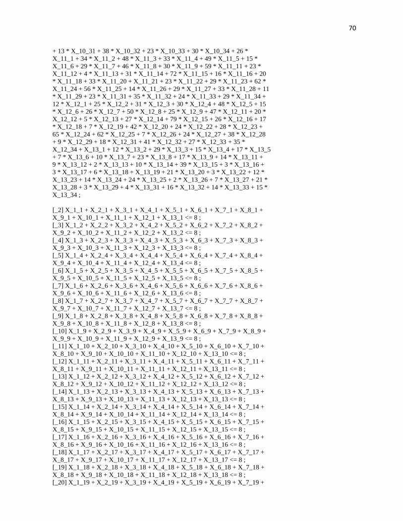
70
+ 13 * X_10_31 + 38 * X_10_32 + 23 * X_10_33 + 30 * X_10_34 + 26 *
X_11_1 + 34 * X_11_2 + 48 * X_11_3 + 33 * X_11_4 + 49 * X_11_5 + 15 *
X_11_6 + 29 * X_11_7 + 46 * X_11_8 + 30 * X_11_9 + 59 * X_11_11 + 23 *
X_11_12 + 4 * X_11_13 + 31 * X_11_14 + 72 * X_11_15 + 16 * X_11_16 + 20
* X_11_18 + 33 * X_11_20 + X_11_21 + 23 * X_11_22 + 29 * X_11_23 + 62 *
X_11_24 + 56 * X_11_25 + 14 * X_11_26 + 29 * X_11_27 + 33 * X_11_28 + 11
* X_11_29 + 23 * X_11_31 + 35 * X_11_32 + 24 * X_11_33 + 29 * X_11_34 +
12 * X_12_1 + 25 * X_12_2 + 31 * X_12_3 + 30 * X_12_4 + 48 * X_12_5 + 15
* X_12_6 + 26 * X_12_7 + 50 * X_12_8 + 25 * X_12_9 + 47 * X_12_11 + 20 *
X_12_12 + 5 * X_12_13 + 27 * X_12_14 + 79 * X_12_15 + 26 * X_12_16 + 17
* X_12_18 + 7 * X_12_19 + 42 * X_12_20 + 24 * X_12_22 + 28 * X_12_23 +
65 * X_12_24 + 62 * X_12_25 + 7 * X_12_26 + 24 * X_12_27 + 38 * X_12_28
+ 9 * X_12_29 + 18 * X_12_31 + 41 * X_12_32 + 27 * X_12_33 + 35 *
X_12_34 + X_13_1 + 12 * X_13_2 + 29 * X_13_3 + 15 * X_13_4 + 17 * X_13_5
+ 7 * X_13_6 + 10 * X_13_7 + 23 * X_13_8 + 17 * X_13_9 + 14 * X_13_11 +
9 * X_13_12 + 2 * X_13_13 + 10 * X_13_14 + 39 * X_13_15 + 3 * X_13_16 +
3 * X_13_17 + 6 * X_13_18 + X_13_19 + 21 * X_13_20 + 3 * X_13_22 + 12 *
X_13_23 + 14 * X_13_24 + 24 * X_13_25 + 2 * X_13_26 + 7 * X_13_27 + 21 *
X_13_28 + 3 * X_13_29 + 4 * X_13_31 + 16 * X_13_32 + 14 * X_13_33 + 15 *
X_13_34 ;
[_2] X_1_1 + X_2_1 + X_3_1 + X_4_1 + X_5_1 + X_6_1 + X_7_1 + X_8_1 +
X_9_1 + X_10_1 + X_11_1 + X_12_1 + X_13_1 <= 8 ;
[_3] X_1_2 + X_2_2 + X_3_2 + X_4_2 + X_5_2 + X_6_2 + X_7_2 + X_8_2 +
X_9_2 + X_10_2 + X_11_2 + X_12_2 + X_13_2 <= 8 ;
[_4] X_1_3 + X_2_3 + X_3_3 + X_4_3 + X_5_3 + X_6_3 + X_7_3 + X_8_3 +
X_9_3 + X_10_3 + X_11_3 + X_12_3 + X_13_3 <= 8 ;
[_5] X_1_4 + X_2_4 + X_3_4 + X_4_4 + X_5_4 + X_6_4 + X_7_4 + X_8_4 +
X_9_4 + X_10_4 + X_11_4 + X_12_4 + X_13_4 <= 8 ;
[_6] X_1_5 + X_2_5 + X_3_5 + X_4_5 + X_5_5 + X_6_5 + X_7_5 + X_8_5 +
X_9_5 + X_10_5 + X_11_5 + X_12_5 + X_13_5 <= 8 ;
[_7] X_1_6 + X_2_6 + X_3_6 + X_4_6 + X_5_6 + X_6_6 + X_7_6 + X_8_6 +
X_9_6 + X_10_6 + X_11_6 + X_12_6 + X_13_6 <= 8 ;
[_8] X_1_7 + X_2_7 + X_3_7 + X_4_7 + X_5_7 + X_6_7 + X_7_7 + X_8_7 +
X_9_7 + X_10_7 + X_11_7 + X_12_7 + X_13_7 <= 8 ;
[_9] X_1_8 + X_2_8 + X_3_8 + X_4_8 + X_5_8 + X_6_8 + X_7_8 + X_8_8 +
X_9_8 + X_10_8 + X_11_8 + X_12_8 + X_13_8 <= 8 ;
[_10] X_1_9 + X_2_9 + X_3_9 + X_4_9 + X_5_9 + X_6_9 + X_7_9 + X_8_9 +
X_9_9 + X_10_9 + X_11_9 + X_12_9 + X_13_9 <= 8 ;
[_11] X_1_10 + X_2_10 + X_3_10 + X_4_10 + X_5_10 + X_6_10 + X_7_10 +
X_8_10 + X_9_10 + X_10_10 + X_11_10 + X_12_10 + X_13_10 <= 8 ;
[_12] X_1_11 + X_2_11 + X_3_11 + X_4_11 + X_5_11 + X_6_11 + X_7_11 +
X_8_11 + X_9_11 + X_10_11 + X_11_11 + X_12_11 + X_13_11 <= 8 ;
[_13] X_1_12 + X_2_12 + X_3_12 + X_4_12 + X_5_12 + X_6_12 + X_7_12 +
X_8_12 + X_9_12 + X_10_12 + X_11_12 + X_12_12 + X_13_12 <= 8 ;
[_14] X_1_13 + X_2_13 + X_3_13 + X_4_13 + X_5_13 + X_6_13 + X_7_13 +
X_8_13 + X_9_13 + X_10_13 + X_11_13 + X_12_13 + X_13_13 <= 8 ;
[_15] X_1_14 + X_2_14 + X_3_14 + X_4_14 + X_5_14 + X_6_14 + X_7_14 +
X_8_14 + X_9_14 + X_10_14 + X_11_14 + X_12_14 + X_13_14 <= 8 ;
[_16] X_1_15 + X_2_15 + X_3_15 + X_4_15 + X_5_15 + X_6_15 + X_7_15 +
X_8_15 + X_9_15 + X_10_15 + X_11_15 + X_12_15 + X_13_15 <= 8 ;
[_17] X_1_16 + X_2_16 + X_3_16 + X_4_16 + X_5_16 + X_6_16 + X_7_16 +
X_8_16 + X_9_16 + X_10_16 + X_11_16 + X_12_16 + X_13_16 <= 8 ;
[_18] X_1_17 + X_2_17 + X_3_17 + X_4_17 + X_5_17 + X_6_17 + X_7_17 +
X_8_17 + X_9_17 + X_10_17 + X_11_17 + X_12_17 + X_13_17 <= 8 ;
[_19] X_1_18 + X_2_18 + X_3_18 + X_4_18 + X_5_18 + X_6_18 + X_7_18 +
X_8_18 + X_9_18 + X_10_18 + X_11_18 + X_12_18 + X_13_18 <= 8 ;
[_20] X_1_19 + X_2_19 + X_3_19 + X_4_19 + X_5_19 + X_6_19 + X_7_19 +

71
X_8_19 + X_9_19 + X_10_19 + X_11_19 + X_12_19 + X_13_19 <= 8 ;
[_21] X_1_20 + X_2_20 + X_3_20 + X_4_20 + X_5_20 + X_6_20 + X_7_20 +
X_8_20 + X_9_20 + X_10_20 + X_11_20 + X_12_20 + X_13_20 <= 8 ;
[_22] X_1_21 + X_2_21 + X_3_21 + X_4_21 + X_5_21 + X_6_21 + X_7_21 +
X_8_21 + X_9_21 + X_10_21 + X_11_21 + X_12_21 + X_13_21 <= 8 ;
[_23] X_1_22 + X_2_22 + X_3_22 + X_4_22 + X_5_22 + X_6_22 + X_7_22 +
X_8_22 + X_9_22 + X_10_22 + X_11_22 + X_12_22 + X_13_22 <= 8 ;
[_24] X_1_23 + X_2_23 + X_3_23 + X_4_23 + X_5_23 + X_6_23 + X_7_23 +
X_8_23 + X_9_23 + X_10_23 + X_11_23 + X_12_23 + X_13_23 <= 8 ;
[_25] X_1_24 + X_2_24 + X_3_24 + X_4_24 + X_5_24 + X_6_24 + X_7_24 +
X_8_24 + X_9_24 + X_10_24 + X_11_24 + X_12_24 + X_13_24 <= 8 ;
[_26] X_1_25 + X_2_25 + X_3_25 + X_4_25 + X_5_25 + X_6_25 + X_7_25 +
X_8_25 + X_9_25 + X_10_25 + X_11_25 + X_12_25 + X_13_25 <= 8 ;
[_27] X_1_26 + X_2_26 + X_3_26 + X_4_26 + X_5_26 + X_6_26 + X_7_26 +
X_8_26 + X_9_26 + X_10_26 + X_11_26 + X_12_26 + X_13_26 <= 8 ;
[_28] X_1_27 + X_2_27 + X_3_27 + X_4_27 + X_5_27 + X_6_27 + X_7_27 +
X_8_27 + X_9_27 + X_10_27 + X_11_27 + X_12_27 + X_13_27 <= 8 ;
[_29] X_1_28 + X_2_28 + X_3_28 + X_4_28 + X_5_28 + X_6_28 + X_7_28 +
X_8_28 + X_9_28 + X_10_28 + X_11_28 + X_12_28 + X_13_28 <= 8 ;
[_30] X_1_29 + X_2_29 + X_3_29 + X_4_29 + X_5_29 + X_6_29 + X_7_29 +
X_8_29 + X_9_29 + X_10_29 + X_11_29 + X_12_29 + X_13_29 <= 8 ;
[_31] X_1_30 + X_2_30 + X_3_30 + X_4_30 + X_5_30 + X_6_30 + X_7_30 +
X_8_30 + X_9_30 + X_10_30 + X_11_30 + X_12_30 + X_13_30 <= 8 ;
[_32] X_1_31 + X_2_31 + X_3_31 + X_4_31 + X_5_31 + X_6_31 + X_7_31 +
X_8_31 + X_9_31 + X_10_31 + X_11_31 + X_12_31 + X_13_31 <= 8 ;
[_33] X_1_32 + X_2_32 + X_3_32 + X_4_32 + X_5_32 + X_6_32 + X_7_32 +
X_8_32 + X_9_32 + X_10_32 + X_11_32 + X_12_32 + X_13_32 <= 8 ;
[_34] X_1_33 + X_2_33 + X_3_33 + X_4_33 + X_5_33 + X_6_33 + X_7_33 +
X_8_33 + X_9_33 + X_10_33 + X_11_33 + X_12_33 + X_13_33 <= 8 ;
[_35] X_1_34 + X_2_34 + X_3_34 + X_4_34 + X_5_34 + X_6_34 + X_7_34 +
X_8_34 + X_9_34 + X_10_34 + X_11_34 + X_12_34 + X_13_34 <= 8 ;
[_36] X_1_1 + X_2_1 + X_3_1 + X_4_1 + X_5_1 + X_6_1 + X_7_1 + X_8_1 +
X_9_1 + X_10_1 + X_11_1 + X_12_1 + X_13_1 >= 0 ;
[_37] X_1_2 + X_2_2 + X_3_2 + X_4_2 + X_5_2 + X_6_2 + X_7_2 + X_8_2 +
X_9_2 + X_10_2 + X_11_2 + X_12_2 + X_13_2 >= 0 ;
[_38] X_1_3 + X_2_3 + X_3_3 + X_4_3 + X_5_3 + X_6_3 + X_7_3 + X_8_3 +
X_9_3 + X_10_3 + X_11_3 + X_12_3 + X_13_3 >= 0 ;
[_39] X_1_4 + X_2_4 + X_3_4 + X_4_4 + X_5_4 + X_6_4 + X_7_4 + X_8_4 +
X_9_4 + X_10_4 + X_11_4 + X_12_4 + X_13_4 >= 0 ;
[_40] X_1_5 + X_2_5 + X_3_5 + X_4_5 + X_5_5 + X_6_5 + X_7_5 + X_8_5 +
X_9_5 + X_10_5 + X_11_5 + X_12_5 + X_13_5 >= 0 ;
[_41] X_1_6 + X_2_6 + X_3_6 + X_4_6 + X_5_6 + X_6_6 + X_7_6 + X_8_6 +
X_9_6 + X_10_6 + X_11_6 + X_12_6 + X_13_6 >= 0 ;
[_42] X_1_7 + X_2_7 + X_3_7 + X_4_7 + X_5_7 + X_6_7 + X_7_7 + X_8_7 +
X_9_7 + X_10_7 + X_11_7 + X_12_7 + X_13_7 >= 0 ;
[_43] X_1_8 + X_2_8 + X_3_8 + X_4_8 + X_5_8 + X_6_8 + X_7_8 + X_8_8 +
X_9_8 + X_10_8 + X_11_8 + X_12_8 + X_13_8 >= 0 ;
[_44] X_1_9 + X_2_9 + X_3_9 + X_4_9 + X_5_9 + X_6_9 + X_7_9 + X_8_9 +
X_9_9 + X_10_9 + X_11_9 + X_12_9 + X_13_9 >= 0 ;
[_45] X_1_10 + X_2_10 + X_3_10 + X_4_10 + X_5_10 + X_6_10 + X_7_10 +
X_8_10 + X_9_10 + X_10_10 + X_11_10 + X_12_10 + X_13_10 >= 0 ;
[_46] X_1_11 + X_2_11 + X_3_11 + X_4_11 + X_5_11 + X_6_11 + X_7_11 +
X_8_11 + X_9_11 + X_10_11 + X_11_11 + X_12_11 + X_13_11 >= 0 ;
[_47] X_1_12 + X_2_12 + X_3_12 + X_4_12 + X_5_12 + X_6_12 + X_7_12 +
X_8_12 + X_9_12 + X_10_12 + X_11_12 + X_12_12 + X_13_12 >= 0 ;
[_48] X_1_13 + X_2_13 + X_3_13 + X_4_13 + X_5_13 + X_6_13 + X_7_13 +
X_8_13 + X_9_13 + X_10_13 + X_11_13 + X_12_13 + X_13_13 >= 0 ;
[_49] X_1_14 + X_2_14 + X_3_14 + X_4_14 + X_5_14 + X_6_14 + X_7_14 +

72
X_8_14 + X_9_14 + X_10_14 + X_11_14 + X_12_14 + X_13_14 >= 0 ;
[_50] X_1_15 + X_2_15 + X_3_15 + X_4_15 + X_5_15 + X_6_15 + X_7_15 +
X_8_15 + X_9_15 + X_10_15 + X_11_15 + X_12_15 + X_13_15 >= 0 ;
[_51] X_1_16 + X_2_16 + X_3_16 + X_4_16 + X_5_16 + X_6_16 + X_7_16 +
X_8_16 + X_9_16 + X_10_16 + X_11_16 + X_12_16 + X_13_16 >= 0 ;
[_52] X_1_17 + X_2_17 + X_3_17 + X_4_17 + X_5_17 + X_6_17 + X_7_17 +
X_8_17 + X_9_17 + X_10_17 + X_11_17 + X_12_17 + X_13_17 >= 0 ;
[_53] X_1_18 + X_2_18 + X_3_18 + X_4_18 + X_5_18 + X_6_18 + X_7_18 +
X_8_18 + X_9_18 + X_10_18 + X_11_18 + X_12_18 + X_13_18 >= 0 ;
[_54] X_1_19 + X_2_19 + X_3_19 + X_4_19 + X_5_19 + X_6_19 + X_7_19 +
X_8_19 + X_9_19 + X_10_19 + X_11_19 + X_12_19 + X_13_19 >= 0 ;
[_55] X_1_20 + X_2_20 + X_3_20 + X_4_20 + X_5_20 + X_6_20 + X_7_20 +
X_8_20 + X_9_20 + X_10_20 + X_11_20 + X_12_20 + X_13_20 >= 0 ;
[_56] X_1_21 + X_2_21 + X_3_21 + X_4_21 + X_5_21 + X_6_21 + X_7_21 +
X_8_21 + X_9_21 + X_10_21 + X_11_21 + X_12_21 + X_13_21 >= 0 ;
[_57] X_1_22 + X_2_22 + X_3_22 + X_4_22 + X_5_22 + X_6_22 + X_7_22 +
X_8_22 + X_9_22 + X_10_22 + X_11_22 + X_12_22 + X_13_22 >= 0 ;
[_58] X_1_23 + X_2_23 + X_3_23 + X_4_23 + X_5_23 + X_6_23 + X_7_23 +
X_8_23 + X_9_23 + X_10_23 + X_11_23 + X_12_23 + X_13_23 >= 0 ;
[_59] X_1_24 + X_2_24 + X_3_24 + X_4_24 + X_5_24 + X_6_24 + X_7_24 +
X_8_24 + X_9_24 + X_10_24 + X_11_24 + X_12_24 + X_13_24 >= 0 ;
[_60] X_1_25 + X_2_25 + X_3_25 + X_4_25 + X_5_25 + X_6_25 + X_7_25 +
X_8_25 + X_9_25 + X_10_25 + X_11_25 + X_12_25 + X_13_25 >= 0 ;
[_61] X_1_26 + X_2_26 + X_3_26 + X_4_26 + X_5_26 + X_6_26 + X_7_26 +
X_8_26 + X_9_26 + X_10_26 + X_11_26 + X_12_26 + X_13_26 >= 0 ;
[_62] X_1_27 + X_2_27 + X_3_27 + X_4_27 + X_5_27 + X_6_27 + X_7_27 +
X_8_27 + X_9_27 + X_10_27 + X_11_27 + X_12_27 + X_13_27 >= 0 ;
[_63] X_1_28 + X_2_28 + X_3_28 + X_4_28 + X_5_28 + X_6_28 + X_7_28 +
X_8_28 + X_9_28 + X_10_28 + X_11_28 + X_12_28 + X_13_28 >= 0 ;
[_64] X_1_29 + X_2_29 + X_3_29 + X_4_29 + X_5_29 + X_6_29 + X_7_29 +
X_8_29 + X_9_29 + X_10_29 + X_11_29 + X_12_29 + X_13_29 >= 0 ;
[_65] X_1_30 + X_2_30 + X_3_30 + X_4_30 + X_5_30 + X_6_30 + X_7_30 +
X_8_30 + X_9_30 + X_10_30 + X_11_30 + X_12_30 + X_13_30 >= 0 ;
[_66] X_1_31 + X_2_31 + X_3_31 + X_4_31 + X_5_31 + X_6_31 + X_7_31 +
X_8_31 + X_9_31 + X_10_31 + X_11_31 + X_12_31 + X_13_31 >= 0 ;
[_67] X_1_32 + X_2_32 + X_3_32 + X_4_32 + X_5_32 + X_6_32 + X_7_32 +
X_8_32 + X_9_32 + X_10_32 + X_11_32 + X_12_32 + X_13_32 >= 0 ;
[_68] X_1_33 + X_2_33 + X_3_33 + X_4_33 + X_5_33 + X_6_33 + X_7_33 +
X_8_33 + X_9_33 + X_10_33 + X_11_33 + X_12_33 + X_13_33 >= 0 ;
[_69] X_1_34 + X_2_34 + X_3_34 + X_4_34 + X_5_34 + X_6_34 + X_7_34 +
X_8_34 + X_9_34 + X_10_34 + X_11_34 + X_12_34 + X_13_34 >= 0 ;
[_70] X_1_1 + X_1_2 + X_1_3 + X_1_4 + X_1_5 + X_1_6 + X_1_7 + X_1_8 +
X_1_9 + X_1_10 + X_1_11 + X_1_12 + X_1_13 + X_1_14 + X_1_15 + X_1_16 +
X_1_17 + X_1_18 + X_1_19 + X_1_20 + X_1_21 + X_1_22 + X_1_23 + X_1_24 +
X_1_25 + X_1_26 + X_1_27 + X_1_28 + X_1_29 + X_1_30 + X_1_31 + X_1_32 +
X_1_33 + X_1_34 <= 3 ;
[_71] X_2_1 + X_2_2 + X_2_3 + X_2_4 + X_2_5 + X_2_6 + X_2_7 + X_2_8 +
X_2_9 + X_2_10 + X_2_11 + X_2_12 + X_2_13 + X_2_14 + X_2_15 + X_2_16 +
X_2_17 + X_2_18 + X_2_19 + X_2_20 + X_2_21 + X_2_22 + X_2_23 + X_2_24 +
X_2_25 + X_2_26 + X_2_27 + X_2_28 + X_2_29 + X_2_30 + X_2_31 + X_2_32 +
X_2_33 + X_2_34 <= 5 ;
[_72] X_3_1 + X_3_2 + X_3_3 + X_3_4 + X_3_5 + X_3_6 + X_3_7 + X_3_8 +
X_3_9 + X_3_10 + X_3_11 + X_3_12 + X_3_13 + X_3_14 + X_3_15 + X_3_16 +
X_3_17 + X_3_18 + X_3_19 + X_3_20 + X_3_21 + X_3_22 + X_3_23 + X_3_24 +
X_3_25 + X_3_26 + X_3_27 + X_3_28 + X_3_29 + X_3_30 + X_3_31 + X_3_32 +
X_3_33 + X_3_34 <= 5 ;
[_73] X_4_1 + X_4_2 + X_4_3 + X_4_4 + X_4_5 + X_4_6 + X_4_7 + X_4_8 +
X_4_9 + X_4_10 + X_4_11 + X_4_12 + X_4_13 + X_4_14 + X_4_15 + X_4_16 +
73
X_4_17 + X_4_18 + X_4_19 + X_4_20 + X_4_21 + X_4_22 + X_4_23 + X_4_24 +
X_4_25 + X_4_26 + X_4_27 + X_4_28 + X_4_29 + X_4_30 + X_4_31 + X_4_32 +
X_4_33 + X_4_34 <= 7 ;
[_74] X_5_1 + X_5_2 + X_5_3 + X_5_4 + X_5_5 + X_5_6 + X_5_7 + X_5_8 +
X_5_9 + X_5_10 + X_5_11 + X_5_12 + X_5_13 + X_5_14 + X_5_15 + X_5_16 +
X_5_17 + X_5_18 + X_5_19 + X_5_20 + X_5_21 + X_5_22 + X_5_23 + X_5_24 +
X_5_25 + X_5_26 + X_5_27 + X_5_28 + X_5_29 + X_5_30 + X_5_31 + X_5_32 +
X_5_33 + X_5_34 <= 7 ;
[_75] X_6_1 + X_6_2 + X_6_3 + X_6_4 + X_6_5 + X_6_6 + X_6_7 + X_6_8 +
X_6_9 + X_6_10 + X_6_11 + X_6_12 + X_6_13 + X_6_14 + X_6_15 + X_6_16 +
X_6_17 + X_6_18 + X_6_19 + X_6_20 + X_6_21 + X_6_22 + X_6_23 + X_6_24 +
X_6_25 + X_6_26 + X_6_27 + X_6_28 + X_6_29 + X_6_30 + X_6_31 + X_6_32 +
X_6_33 + X_6_34 <= 7 ;
[_76] X_7_1 + X_7_2 + X_7_3 + X_7_4 + X_7_5 + X_7_6 + X_7_7 + X_7_8 +
X_7_9 + X_7_10 + X_7_11 + X_7_12 + X_7_13 + X_7_14 + X_7_15 + X_7_16 +
X_7_17 + X_7_18 + X_7_19 + X_7_20 + X_7_21 + X_7_22 + X_7_23 + X_7_24 +
X_7_25 + X_7_26 + X_7_27 + X_7_28 + X_7_29 + X_7_30 + X_7_31 + X_7_32 +
X_7_33 + X_7_34 <= 5 ;
[_77] X_8_1 + X_8_2 + X_8_3 + X_8_4 + X_8_5 + X_8_6 + X_8_7 + X_8_8 +
X_8_9 + X_8_10 + X_8_11 + X_8_12 + X_8_13 + X_8_14 + X_8_15 + X_8_16 +
X_8_17 + X_8_18 + X_8_19 + X_8_20 + X_8_21 + X_8_22 + X_8_23 + X_8_24 +
X_8_25 + X_8_26 + X_8_27 + X_8_28 + X_8_29 + X_8_30 + X_8_31 + X_8_32 +
X_8_33 + X_8_34 <= 5 ;
[_78] X_9_1 + X_9_2 + X_9_3 + X_9_4 + X_9_5 + X_9_6 + X_9_7 + X_9_8 +
X_9_9 + X_9_10 + X_9_11 + X_9_12 + X_9_13 + X_9_14 + X_9_15 + X_9_16 +
X_9_17 + X_9_18 + X_9_19 + X_9_20 + X_9_21 + X_9_22 + X_9_23 + X_9_24 +
X_9_25 + X_9_26 + X_9_27 + X_9_28 + X_9_29 + X_9_30 + X_9_31 + X_9_32 +
X_9_33 + X_9_34 <= 7 ;
[_79] X_10_1 + X_10_2 + X_10_3 + X_10_4 + X_10_5 + X_10_6 + X_10_7 +
X_10_8 + X_10_9 + X_10_10 + X_10_11 + X_10_12 + X_10_13 + X_10_14 +
X_10_15 + X_10_16 + X_10_17 + X_10_18 + X_10_19 + X_10_20 + X_10_21 +
X_10_22 + X_10_23 + X_10_24 + X_10_25 + X_10_26 + X_10_27 + X_10_28 +
X_10_29 + X_10_30 + X_10_31 + X_10_32 + X_10_33 + X_10_34 <= 7 ;
[_80] X_11_1 + X_11_2 + X_11_3 + X_11_4 + X_11_5 + X_11_6 + X_11_7 +
X_11_8 + X_11_9 + X_11_10 + X_11_11 + X_11_12 + X_11_13 + X_11_14 +
X_11_15 + X_11_16 + X_11_17 + X_11_18 + X_11_19 + X_11_20 + X_11_21 +
X_11_22 + X_11_23 + X_11_24 + X_11_25 + X_11_26 + X_11_27 + X_11_28 +
X_11_29 + X_11_30 + X_11_31 + X_11_32 + X_11_33 + X_11_34 <= 7 ;
[_81] X_12_1 + X_12_2 + X_12_3 + X_12_4 + X_12_5 + X_12_6 + X_12_7 +
X_12_8 + X_12_9 + X_12_10 + X_12_11 + X_12_12 + X_12_13 + X_12_14 +
X_12_15 + X_12_16 + X_12_17 + X_12_18 + X_12_19 + X_12_20 + X_12_21 +
X_12_22 + X_12_23 + X_12_24 + X_12_25 + X_12_26 + X_12_27 + X_12_28 +
X_12_29 + X_12_30 + X_12_31 + X_12_32 + X_12_33 + X_12_34 <= 6 ;
[_82] X_13_1 + X_13_2 + X_13_3 + X_13_4 + X_13_5 + X_13_6 + X_13_7 +
X_13_8 + X_13_9 + X_13_10 + X_13_11 + X_13_12 + X_13_13 + X_13_14 +
X_13_15 + X_13_16 + X_13_17 + X_13_18 + X_13_19 + X_13_20 + X_13_21 +
X_13_22 + X_13_23 + X_13_24 + X_13_25 + X_13_26 + X_13_27 + X_13_28 +
X_13_29 + X_13_30 + X_13_31 + X_13_32 + X_13_33 + X_13_34 <= 3 ;
[_83] X_1_1 + X_1_2 + X_1_3 + X_1_4 + X_1_5 + X_1_6 + X_1_7 + X_1_8 +
X_1_9 + X_1_10 + X_1_11 + X_1_12 + X_1_13 + X_1_14 + X_1_15 + X_1_16 +
X_1_17 + X_1_18 + X_1_19 + X_1_20 + X_1_21 + X_1_22 + X_1_23 + X_1_24 +
X_1_25 + X_1_26 + X_1_27 + X_1_28 + X_1_29 + X_1_30 + X_1_31 + X_1_32 +
X_1_33 + X_1_34 >= 1 ;
[_84] X_2_1 + X_2_2 + X_2_3 + X_2_4 + X_2_5 + X_2_6 + X_2_7 + X_2_8 +
X_2_9 + X_2_10 + X_2_11 + X_2_12 + X_2_13 + X_2_14 + X_2_15 + X_2_16 +
X_2_17 + X_2_18 + X_2_19 + X_2_20 + X_2_21 + X_2_22 + X_2_23 + X_2_24 +
X_2_25 + X_2_26 + X_2_27 + X_2_28 + X_2_29 + X_2_30 + X_2_31 + X_2_32 +
X_2_33 + X_2_34 >= 3 ;
74
[_85] X_3_1 + X_3_2 + X_3_3 + X_3_4 + X_3_5 + X_3_6 + X_3_7 + X_3_8 +
X_3_9 + X_3_10 + X_3_11 + X_3_12 + X_3_13 + X_3_14 + X_3_15 + X_3_16 +
X_3_17 + X_3_18 + X_3_19 + X_3_20 + X_3_21 + X_3_22 + X_3_23 + X_3_24 +
X_3_25 + X_3_26 + X_3_27 + X_3_28 + X_3_29 + X_3_30 + X_3_31 + X_3_32 +
X_3_33 + X_3_34 >= 3 ;
[_86] X_4_1 + X_4_2 + X_4_3 + X_4_4 + X_4_5 + X_4_6 + X_4_7 + X_4_8 +
X_4_9 + X_4_10 + X_4_11 + X_4_12 + X_4_13 + X_4_14 + X_4_15 + X_4_16 +
X_4_17 + X_4_18 + X_4_19 + X_4_20 + X_4_21 + X_4_22 + X_4_23 + X_4_24 +
X_4_25 + X_4_26 + X_4_27 + X_4_28 + X_4_29 + X_4_30 + X_4_31 + X_4_32 +
X_4_33 + X_4_34 >= 5 ;
[_87] X_5_1 + X_5_2 + X_5_3 + X_5_4 + X_5_5 + X_5_6 + X_5_7 + X_5_8 +
X_5_9 + X_5_10 + X_5_11 + X_5_12 + X_5_13 + X_5_14 + X_5_15 + X_5_16 +
X_5_17 + X_5_18 + X_5_19 + X_5_20 + X_5_21 + X_5_22 + X_5_23 + X_5_24 +
X_5_25 + X_5_26 + X_5_27 + X_5_28 + X_5_29 + X_5_30 + X_5_31 + X_5_32 +
X_5_33 + X_5_34 >= 5 ;
[_88] X_6_1 + X_6_2 + X_6_3 + X_6_4 + X_6_5 + X_6_6 + X_6_7 + X_6_8 +
X_6_9 + X_6_10 + X_6_11 + X_6_12 + X_6_13 + X_6_14 + X_6_15 + X_6_16 +
X_6_17 + X_6_18 + X_6_19 + X_6_20 + X_6_21 + X_6_22 + X_6_23 + X_6_24 +
X_6_25 + X_6_26 + X_6_27 + X_6_28 + X_6_29 + X_6_30 + X_6_31 + X_6_32 +
X_6_33 + X_6_34 >= 5 ;
[_89] X_7_1 + X_7_2 + X_7_3 + X_7_4 + X_7_5 + X_7_6 + X_7_7 + X_7_8 +
X_7_9 + X_7_10 + X_7_11 + X_7_12 + X_7_13 + X_7_14 + X_7_15 + X_7_16 +
X_7_17 + X_7_18 + X_7_19 + X_7_20 + X_7_21 + X_7_22 + X_7_23 + X_7_24 +
X_7_25 + X_7_26 + X_7_27 + X_7_28 + X_7_29 + X_7_30 + X_7_31 + X_7_32 +
X_7_33 + X_7_34 >= 3 ;
[_90] X_8_1 + X_8_2 + X_8_3 + X_8_4 + X_8_5 + X_8_6 + X_8_7 + X_8_8 +
X_8_9 + X_8_10 + X_8_11 + X_8_12 + X_8_13 + X_8_14 + X_8_15 + X_8_16 +
X_8_17 + X_8_18 + X_8_19 + X_8_20 + X_8_21 + X_8_22 + X_8_23 + X_8_24 +
X_8_25 + X_8_26 + X_8_27 + X_8_28 + X_8_29 + X_8_30 + X_8_31 + X_8_32 +
X_8_33 + X_8_34 >= 3 ;
[_91] X_9_1 + X_9_2 + X_9_3 + X_9_4 + X_9_5 + X_9_6 + X_9_7 + X_9_8 +
X_9_9 + X_9_10 + X_9_11 + X_9_12 + X_9_13 + X_9_14 + X_9_15 + X_9_16 +
X_9_17 + X_9_18 + X_9_19 + X_9_20 + X_9_21 + X_9_22 + X_9_23 + X_9_24 +
X_9_25 + X_9_26 + X_9_27 + X_9_28 + X_9_29 + X_9_30 + X_9_31 + X_9_32 +
X_9_33 + X_9_34 >= 5 ;
[_92] X_10_1 + X_10_2 + X_10_3 + X_10_4 + X_10_5 + X_10_6 + X_10_7 +
X_10_8 + X_10_9 + X_10_10 + X_10_11 + X_10_12 + X_10_13 + X_10_14 +
X_10_15 + X_10_16 + X_10_17 + X_10_18 + X_10_19 + X_10_20 + X_10_21 +
X_10_22 + X_10_23 + X_10_24 + X_10_25 + X_10_26 + X_10_27 + X_10_28 +
X_10_29 + X_10_30 + X_10_31 + X_10_32 + X_10_33 + X_10_34 >= 5 ;
[_93] X_11_1 + X_11_2 + X_11_3 + X_11_4 + X_11_5 + X_11_6 + X_11_7 +
X_11_8 + X_11_9 + X_11_10 + X_11_11 + X_11_12 + X_11_13 + X_11_14 +
X_11_15 + X_11_16 + X_11_17 + X_11_18 + X_11_19 + X_11_20 + X_11_21 +
X_11_22 + X_11_23 + X_11_24 + X_11_25 + X_11_26 + X_11_27 + X_11_28 +
X_11_29 + X_11_30 + X_11_31 + X_11_32 + X_11_33 + X_11_34 >= 5 ;
[_94] X_12_1 + X_12_2 + X_12_3 + X_12_4 + X_12_5 + X_12_6 + X_12_7 +
X_12_8 + X_12_9 + X_12_10 + X_12_11 + X_12_12 + X_12_13 + X_12_14 +
X_12_15 + X_12_16 + X_12_17 + X_12_18 + X_12_19 + X_12_20 + X_12_21 +
X_12_22 + X_12_23 + X_12_24 + X_12_25 + X_12_26 + X_12_27 + X_12_28 +
X_12_29 + X_12_30 + X_12_31 + X_12_32 + X_12_33 + X_12_34 >= 4 ;
[_95] X_13_1 + X_13_2 + X_13_3 + X_13_4 + X_13_5 + X_13_6 + X_13_7 +
X_13_8 + X_13_9 + X_13_10 + X_13_11 + X_13_12 + X_13_13 + X_13_14 +
X_13_15 + X_13_16 + X_13_17 + X_13_18 + X_13_19 + X_13_20 + X_13_21 +
X_13_22 + X_13_23 + X_13_24 + X_13_25 + X_13_26 + X_13_27 + X_13_28 +
X_13_29 + X_13_30 + X_13_31 + X_13_32 + X_13_33 + X_13_34 >= 2 ;
@BIN( X_1_1); @BIN( X_1_2); @BIN( X_1_3); @BIN( X_1_4);
@BIN( X_1_5); @BIN( X_1_6); @BIN( X_1_7); @BIN( X_1_8);
@BIN( X_1_9); @BIN( X_1_10); @BIN( X_1_11); @BIN(

75
X_1_12); @BIN( X_1_13); @BIN( X_1_14); @BIN( X_1_15);
@BIN( X_1_16); @BIN( X_1_17); @BIN( X_1_18); @BIN(
X_1_19); @BIN( X_1_20); @BIN( X_1_21); @BIN( X_1_22);
@BIN( X_1_23); @BIN( X_1_24); @BIN( X_1_25); @BIN(
X_1_26); @BIN( X_1_27); @BIN( X_1_28); @BIN( X_1_29);
@BIN( X_1_30); @BIN( X_1_31); @BIN( X_1_32); @BIN(
X_1_33); @BIN( X_1_34); @BIN( X_2_1); @BIN( X_2_2); @BIN(
X_2_3); @BIN( X_2_4); @BIN( X_2_5); @BIN( X_2_6); @BIN(
X_2_7); @BIN( X_2_8); @BIN( X_2_9); @BIN( X_2_10); @BIN(
X_2_11); @BIN( X_2_12); @BIN( X_2_13); @BIN( X_2_14);
@BIN( X_2_15); @BIN( X_2_16); @BIN( X_2_17); @BIN(
X_2_18); @BIN( X_2_19); @BIN( X_2_20); @BIN( X_2_21);
@BIN( X_2_22); @BIN( X_2_23); @BIN( X_2_24); @BIN(
X_2_25); @BIN( X_2_26); @BIN( X_2_27); @BIN( X_2_28);
@BIN( X_2_29); @BIN( X_2_30); @BIN( X_2_31); @BIN(
X_2_32); @BIN( X_2_33); @BIN( X_2_34); @BIN( X_3_1);
@BIN( X_3_2); @BIN( X_3_3); @BIN( X_3_4); @BIN( X_3_5);
@BIN( X_3_6); @BIN( X_3_7); @BIN( X_3_8); @BIN( X_3_9);
@BIN( X_3_10); @BIN( X_3_11); @BIN( X_3_12); @BIN(
X_3_13); @BIN( X_3_14); @BIN( X_3_15); @BIN( X_3_16);
@BIN( X_3_17); @BIN( X_3_18); @BIN( X_3_19); @BIN(
X_3_20); @BIN( X_3_21); @BIN( X_3_22); @BIN( X_3_23);
@BIN( X_3_24); @BIN( X_3_25); @BIN( X_3_26); @BIN(
X_3_27); @BIN( X_3_28); @BIN( X_3_29); @BIN( X_3_30);
@BIN( X_3_31); @BIN( X_3_32); @BIN( X_3_33); @BIN(
X_3_34); @BIN( X_4_1); @BIN( X_4_2); @BIN( X_4_3); @BIN(
X_4_4); @BIN( X_4_5); @BIN( X_4_6); @BIN( X_4_7); @BIN(
X_4_8); @BIN( X_4_9); @BIN( X_4_10); @BIN( X_4_11); @BIN(
X_4_12); @BIN( X_4_13); @BIN( X_4_14); @BIN( X_4_15);
@BIN( X_4_16); @BIN( X_4_17); @BIN( X_4_18); @BIN(
X_4_19); @BIN( X_4_20); @BIN( X_4_21); @BIN( X_4_22);
@BIN( X_4_23); @BIN( X_4_24); @BIN( X_4_25); @BIN(
X_4_26); @BIN( X_4_27); @BIN( X_4_28); @BIN( X_4_29);
@BIN( X_4_30); @BIN( X_4_31); @BIN( X_4_32); @BIN(
X_4_33); @BIN( X_4_34); @BIN( X_5_1); @BIN( X_5_2); @BIN(
X_5_3); @BIN( X_5_4); @BIN( X_5_5); @BIN( X_5_6); @BIN(
X_5_7); @BIN( X_5_8); @BIN( X_5_9); @BIN( X_5_10); @BIN(
X_5_11); @BIN( X_5_12); @BIN( X_5_13); @BIN( X_5_14);
@BIN( X_5_15); @BIN( X_5_16); @BIN( X_5_17); @BIN(
X_5_18); @BIN( X_5_19); @BIN( X_5_20); @BIN( X_5_21);
@BIN( X_5_22); @BIN( X_5_23); @BIN( X_5_24); @BIN(
X_5_25); @BIN( X_5_26); @BIN( X_5_27); @BIN( X_5_28);
@BIN( X_5_29); @BIN( X_5_30); @BIN( X_5_31); @BIN(
X_5_32); @BIN( X_5_33); @BIN( X_5_34); @BIN( X_6_1);
@BIN( X_6_2); @BIN( X_6_3); @BIN( X_6_4); @BIN( X_6_5);
@BIN( X_6_6); @BIN( X_6_7); @BIN( X_6_8); @BIN( X_6_9);
@BIN( X_6_10); @BIN( X_6_11); @BIN( X_6_12); @BIN(
X_6_13); @BIN( X_6_14); @BIN( X_6_15); @BIN( X_6_16);
@BIN( X_6_17); @BIN( X_6_18); @BIN( X_6_19); @BIN(
X_6_20); @BIN( X_6_21); @BIN( X_6_22); @BIN( X_6_23);
@BIN( X_6_24); @BIN( X_6_25); @BIN( X_6_26); @BIN(
X_6_27); @BIN( X_6_28); @BIN( X_6_29); @BIN( X_6_30);
@BIN( X_6_31); @BIN( X_6_32); @BIN( X_6_33); @BIN(
X_6_34); @BIN( X_7_1); @BIN( X_7_2); @BIN( X_7_3); @BIN(
X_7_4); @BIN( X_7_5); @BIN( X_7_6); @BIN( X_7_7); @BIN(
X_7_8); @BIN( X_7_9); @BIN( X_7_10); @BIN( X_7_11); @BIN(
X_7_12); @BIN( X_7_13); @BIN( X_7_14); @BIN( X_7_15);
@BIN( X_7_16); @BIN( X_7_17); @BIN( X_7_18); @BIN(

76
X_7_19); @BIN( X_7_20); @BIN( X_7_21); @BIN( X_7_22);
@BIN( X_7_23); @BIN( X_7_24); @BIN( X_7_25); @BIN(
X_7_26); @BIN( X_7_27); @BIN( X_7_28); @BIN( X_7_29);
@BIN( X_7_30); @BIN( X_7_31); @BIN( X_7_32); @BIN(
X_7_33); @BIN( X_7_34); @BIN( X_8_1); @BIN( X_8_2); @BIN(
X_8_3); @BIN( X_8_4); @BIN( X_8_5); @BIN( X_8_6); @BIN(
X_8_7); @BIN( X_8_8); @BIN( X_8_9); @BIN( X_8_10); @BIN(
X_8_11); @BIN( X_8_12); @BIN( X_8_13); @BIN( X_8_14);
@BIN( X_8_15); @BIN( X_8_16); @BIN( X_8_17); @BIN(
X_8_18); @BIN( X_8_19); @BIN( X_8_20); @BIN( X_8_21);
@BIN( X_8_22); @BIN( X_8_23); @BIN( X_8_24); @BIN(
X_8_25); @BIN( X_8_26); @BIN( X_8_27); @BIN( X_8_28);
@BIN( X_8_29); @BIN( X_8_30); @BIN( X_8_31); @BIN(
X_8_32); @BIN( X_8_33); @BIN( X_8_34); @BIN( X_9_1);
@BIN( X_9_2); @BIN( X_9_3); @BIN( X_9_4); @BIN( X_9_5);
@BIN( X_9_6); @BIN( X_9_7); @BIN( X_9_8); @BIN( X_9_9);
@BIN( X_9_10); @BIN( X_9_11); @BIN( X_9_12); @BIN(
X_9_13); @BIN( X_9_14); @BIN( X_9_15); @BIN( X_9_16);
@BIN( X_9_17); @BIN( X_9_18); @BIN( X_9_19); @BIN(
X_9_20); @BIN( X_9_21); @BIN( X_9_22); @BIN( X_9_23);
@BIN( X_9_24); @BIN( X_9_25); @BIN( X_9_26); @BIN(
X_9_27); @BIN( X_9_28); @BIN( X_9_29); @BIN( X_9_30);
@BIN( X_9_31); @BIN( X_9_32); @BIN( X_9_33); @BIN(
X_9_34); @BIN( X_10_1); @BIN( X_10_2); @BIN( X_10_3);
@BIN( X_10_4); @BIN( X_10_5); @BIN( X_10_6); @BIN(
X_10_7); @BIN( X_10_8); @BIN( X_10_9); @BIN( X_10_10);
@BIN( X_10_11); @BIN( X_10_12); @BIN( X_10_13); @BIN(
X_10_14); @BIN( X_10_15); @BIN( X_10_16); @BIN( X_10_17);
@BIN( X_10_18); @BIN( X_10_19); @BIN( X_10_20); @BIN(
X_10_21); @BIN( X_10_22); @BIN( X_10_23); @BIN( X_10_24);
@BIN( X_10_25); @BIN( X_10_26); @BIN( X_10_27); @BIN(
X_10_28); @BIN( X_10_29); @BIN( X_10_30); @BIN( X_10_31);
@BIN( X_10_32); @BIN( X_10_33); @BIN( X_10_34); @BIN(
X_11_1); @BIN( X_11_2); @BIN( X_11_3); @BIN( X_11_4);
@BIN( X_11_5); @BIN( X_11_6); @BIN( X_11_7); @BIN(
X_11_8); @BIN( X_11_9); @BIN( X_11_10); @BIN( X_11_11);
@BIN( X_11_12); @BIN( X_11_13); @BIN( X_11_14); @BIN(
X_11_15); @BIN( X_11_16); @BIN( X_11_17); @BIN( X_11_18);
@BIN( X_11_19); @BIN( X_11_20); @BIN( X_11_21); @BIN(
X_11_22); @BIN( X_11_23); @BIN( X_11_24); @BIN( X_11_25);
@BIN( X_11_26); @BIN( X_11_27); @BIN( X_11_28); @BIN(
X_11_29); @BIN( X_11_30); @BIN( X_11_31); @BIN( X_11_32);
@BIN( X_11_33); @BIN( X_11_34); @BIN( X_12_1); @BIN(
X_12_2); @BIN( X_12_3); @BIN( X_12_4); @BIN( X_12_5);
@BIN( X_12_6); @BIN( X_12_7); @BIN( X_12_8); @BIN(
X_12_9); @BIN( X_12_10); @BIN( X_12_11); @BIN( X_12_12);
@BIN( X_12_13); @BIN( X_12_14); @BIN( X_12_15); @BIN(
X_12_16); @BIN( X_12_17); @BIN( X_12_18); @BIN( X_12_19);
@BIN( X_12_20); @BIN( X_12_21); @BIN( X_12_22); @BIN(
X_12_23); @BIN( X_12_24); @BIN( X_12_25); @BIN( X_12_26);
@BIN( X_12_27); @BIN( X_12_28); @BIN( X_12_29); @BIN(
X_12_30); @BIN( X_12_31); @BIN( X_12_32); @BIN( X_12_33);
@BIN( X_12_34); @BIN( X_13_1); @BIN( X_13_2); @BIN(
X_13_3); @BIN( X_13_4); @BIN( X_13_5); @BIN( X_13_6);
@BIN( X_13_7); @BIN( X_13_8); @BIN( X_13_9); @BIN(
X_13_10); @BIN( X_13_11); @BIN( X_13_12); @BIN( X_13_13);
@BIN( X_13_14); @BIN( X_13_15); @BIN( X_13_16); @BIN(
X_13_17); @BIN( X_13_18); @BIN( X_13_19); @BIN( X_13_20);

77
@BIN( X_13_21); @BIN( X_13_22); @BIN( X_13_23); @BIN(
X_13_24); @BIN( X_13_25); @BIN( X_13_26); @BIN( X_13_27);
@BIN( X_13_28); @BIN( X_13_29); @BIN( X_13_30); @BIN(
X_13_31); @BIN( X_13_32); @BIN( X_13_33); @BIN( X_13_34);
END

78
Appendix D: Complete Set of Apriori Rules
Table 1: Items bought together
S.No Rules Support Confidence
1 {2088} => {97} 0.24107 0.44876
2 {1382} => {97} 0.113531 0.359627
3 {686} => {97} 0.113952 0.636648
4 {1527} => {1528} 0.2066 0.470426
5 {102} => {17} 0.246206 0.768249
6 {41} => {40} 0.16039 0.8667
7 {40} => {41} 0.16039 0.486605
8 {61} => {17} 0.15997 0.578476
9 {129,160} => {17} 0.14923 0.925797
10 {17,160} => {129} 0.14923 0.867935
11 {17,129} => {160} 0.14923 0.312097
12 {129,132} => {17} 0.13498 0.912508
13 {17,132} => {129} 0.13498 0.79543
14 {1423} => {97} 0.12834 0.785755
15 {846} => {1528} 0.15661 0.544244
16 {1294} => {97} 0.10526 0.760892
17 {1435} => {97} 0.1196 0.784314
18 {1304} => {97} 0.10886 0.591521
19 {2640} => {97} 0.010096 0.574581
20 {822} => {97} 0.12465 0.393278
21 {179} => {56} 0.013049 0.548507
22 {82} => {17} 0.010143 0.505825
23 {846} => {97} 0.010881 0.378146
24 {98} => {97} 0.1047 0.332591
25 {2025} => {97} 0.01347 0.693029
26 {1951} => {97} 0.012928 0.632602
27 {102} => {97} 0.0287846 0.319554
28 {1528} => {97} 0.030177 0.356064
29 {60} => {17} 0.01076 0.687668
30 {40} => {17} 0.011026 0.334515
31 {1} => {129} 0.11816 0.860204
32 {1} => {17} 0.012423 0.904422
33 {135} => {54} 0.01125 0.363417
34 {135} => {17} 0.015862 0.512375
35 {72} => {54} 0.011255 0.463537
36 {72} => {17} 0.017539 0.72234
37 {170} => {129} 0.0124 0.608995
38 {170} => {17} 0.01681 0.825608
39 {168} => {129} 0.012031 0.565189
40 {168} => {17} 0.016226 0.762291

79
41 {106} => {17} 0.016628 0.665981
42 {11} => {129} 0.011049 0.514242
43 {11} => {17} 0.015899 0.739943
44 {160} => {129} 0.016119 0.866399
45 {129} => {160} 0.016119 0.306667
46 {160} => {17} 0.017193 0.924159
47 {132} => {129} 0.14792 0.752019
48 {132} => {17} 0.016969 0.862708
49 {137} => {17} 0.018651 0.652607
50 {9} => {129} 0.016983 0.867128
51 {129} => {9} 0.016983 0.323111
52 {9} => {17} 0.017179 0.877147
53 {15} => {17} 0.015955 0.61135
54 {45} => {17} 0.027832 0.418241
55 {10} => {129} 0.019132 0.861199
56 {129} => {10} 0.019132 0.364
57 {10} => {17} 0.01994 0.897581
58 {139} => {54} 0.013035 0.316219
59 {139} => {17} 0.025509 0.618837
60 {167} => {129} 0.013979 0.533048
61 {167} => {17} 0.0193 0.73597
62 {90} => {107} 0.011311 0.334023
63 {90} => {87} 0.012563 0.370999
64 {90} => {54} 0.014399 0.425221
65 {90} => {17} 0.02244 0.662666
66 {13} => {30} 0.014474 0.319975
67 {13} => {17} 0.022772 0.503408
68 {27} => {129} 0.016796 0.404979
69 {129} => {27} 0.016796 0.319556
70 {27} => {17} 0.02322 0.559874
71 {107} => {17} 0.029238 0.527078
72 {65} => {17} 0.032779 0.433944
73 {87} => {54} 0.026878 0.312935
74 {87} => {17} 0.03776 0.439621
75 {129} => {17} 0.047814 0.909689
76 {30} => {17} 0.055808 0.40057
77 {54} => {17} 0.077 0.518989
78 {1,129} => {17} 0.01075 0.909846
79 {1,17} => {129} 0.01075 0.865363
80 {129,170} => {17} 0.011077 0.893369
81 {17,170} => {129} 0.011077 0.658977
82 {129,168} => {17} 0.010849 0.901748
83 {17,168} => {129} 0.010849 0.668586
84 {17,132} => {129} 0.13498 0.79543

80
85 {9,129} => {17} 0.014904 0.877579
86 {9,17} => {129} 0.014904 0.867555
87 {17,129} => {9} 0.014904 0.311706
88 {10,129} => {17} 0.017179 0.897924
89 {10,17} => {129} 0.017179 0.861528
90 {17,129} => {10} 0.017179 0.359293
91 {129,167} => {17} 0.012685 0.90742
92 {17,167} => {129} 0.012685 0.657226
93 {27,129} => {17} 0.014782 0.880111
94 {17,27} => {129} 0.014782 0.63662
95 {17,129} => {27} 0.014782 0.309166
96 {65,129} => {17} 0.013605 0.901827
97 {17,65} => {129} 0.013605 0.415051
98 {54,87} => {17} 0.016226 0.603685
99 {17,87} => {54} 0.016226 0.42972
100 {30,129} => {17} 0.011685 0.855921
101 {30,54} => {17} 0.011951 0.567814