1

A preliminary Landsat MSS-derived land-cover map of

the Seward Peninsula, Alaska: classification methods and comparison with existing data sets

C.R. Thayer-Snyder1, H.A. Maier2 and D.A. Walker2

1Western Washington University, Huxley College of Environmental and Social Sciences, Bellingham, WA

98225 USA. 2Alaska Geobotany Center, Institute of Arctic Biology, University of Alaska Fairbanks, Fairbanks, AK 99775.

3Published: February 2002, Revised: December 2003

ABSTRACT Present climate-change and ecosystem research studies in Arctic and Sub-Arctic areas have created a high demand for detailed land-cover maps. I produced a preliminary land-cover map of the Seward Peninsula, Alaska, using Landsat Multi-Spectral Scanner (MSS)-derived imagery. I used a multiple scene mosaic furnished by the USGS, EROS Data Center, and an Isoclass clustering algorithm to arrive at 9 broad land-cover classes. The Seward Peninsula Multi-Spectral Scanner Map (MSS) has the following land-cover classes and respective percentages: Barrens (3.4%); Dry Prostrate Dwarf-shrub Tundra (6.7%); Moist Herbaceous Dwarf-shrub Tundra (53.7%); Wet Herbaceous Tundra (8.5%); Moist Low-shrub and Tall-shrub Tundra (16.7%); Spruce Forest (5.6%); Water (5.0%); Snow and Clouds (<0.1%); and Shadows (0.5%). Ancillary data including a digital elevation model and previous land-cover maps of the Seward Peninsula were used to make improvements to the MSS land-cover classifications. The MSS map gives a high level of spatial detail that is unequaled by the comparison data sets: the Major Ecosystems of Alaska (MEA) map, and the Seward Peninsula Soil Conservation Service (SCS) map. Comparative graphs show the breakdown of land-cover percentages for each of the three data sets. Additionally, difference matrices were calculated, which provide a quantitative indication of how well the land-cover classes of the three data sets overlay each other. The MSS map gives a better representation of the variable spatial distribution of vegetation within the otherwise homogeneous SCS and MEA map land-cover designations. Overall, the high level detail provided by the MSS data set offers a superior map for understanding the complex patterns of vegetation distribution on the Seward Peninsula.

3Originally published as part of “ATLAS Vegetation Studies: Seward Peninsula, Alaska, 2000”, ARCCS-ATLAS-AGC Data Report, February 2002. Original report was prepared by C.R. Thayer-Snyder as part of a Research Experience for Undergraduates project (NSF grant OPP-990829). Revisions made December 2003 by the Alaska Geobotany Center.

2

INTRODUCTION

Present climate change and ecosystem research studies in Arctic and Sub-Arctic areas are creating a high demand for detailed land-cover maps. The MSS-derived Seward Peninsula land-cover map (MSS) was created to supply a detailed land-cover map for two National Science Foundation funded projects: the Arctic Transitions in the Land-Atmosphere System (ATLAS) project, and the Circumpolar Arctic Vegetation Map (CAVM) project (Walker, 1995).

The ATLAS project addresses the role of energy, water vapor, and trace gasses in the Arctic region, and ultimately, how these variables interact with the global-scale climate structure (Rowntree, 1997). When combined with field observations, the MSS map provides a basis for calculating total trace gas fluxes, above and below ground biomass, radiation, and heat flux on the Seward Peninsula.

The goal of the CAVM project is to provide the first detailed vegetation map of the entire circumpolar area (Walker, 1995). When completed, the CAVM map will provide a framework for global-scale climate and ecosystem studies such as the ATLAS project. The Seward MSS map serves as an indication of the effectiveness of integrating Multi-Spectral Scanner data into the overall CAVM project, which relies heavily on Advanced Very High Resolution Radiometer (AVHRR) imagery. Geography of the Seward Peninsula and Study Area

Sometimes referred to as the "nose" of Alaska, the Seward Peninsula is a remote, yet diverse region located in northwestern Alaska. Bordered by the Chukchi Sea to the north, the Bering Strait to the west, and Norton Sound to the south, the Peninsula is surrounded by relatively cold water to the north and west but relatively warm water to the south. The temperature of surrounding water bodies serves as a large determinant to the distribution of land-cover present on the Peninsula. Vegetation types range from dense evergreen forests to the southeast to treeless wet herbaceous tundra to the north.

The study area is defined as the entire Seward Peninsula west of an arbitrary line drawn between the Elephant Point to the north, and the Koyukuk River Delta to the south (Figure 1). The study area is approximately 50,000 square kilometers, roughly double the land area of Vermont. Existing Maps of the Seward Peninsula

I compared the MSS-derived Seward map with two other digital-form maps: The Major Ecosystems of Alaska (MEA) map (Joint Federal State Land Use Planning Commission, 1973) and the Range Survey of the Seward Peninsula Reindeer Ranges, Alaska (U.S. Department of Agriculture's Soil Conservation Service, 1985). I will refer to these maps as the MEA and SCS maps respectively.

3

Figure 1: The Seward Peninsula unsupervised MSS landcover classification.

4

Figure 2. The Major Ecosystems of Alaska map reclassified from seven to six land-cover classes.

Table 1. Crosswalk between original and altered MEA land-cover classes.

Original Name Altered Name Alpine tundra Alpine Tundra Moist tundra Moist Tundra Wet tundra Wet Tundra High brush High Brush Bottomland spruce-poplar forest Spruce Forest Upland spruce-hardwood forest Spruce Forest Water Water

The MEA map is the historic standard for all other vegetation-distribution maps of Alaska (Figure 2). The digital MEA vector based data set is based on a map created by John Spetzman in 1959 (Spetzman, 1959). The MEA data set was digitized from the

Spetzman-derived MEA map in 1991 at a scale of 1:2,500,000. The Seward Peninsula portion of the MEA map contains seven land-cover classes. However, for map comparison, the seven categories were reduced to six (Table 1). Although the MEA data does a good job at conveying the state-wide distribution of vegetation in Alaska, it

is highly generalized due to its small production scale, and is generally not an appropriate base map for current scientific research.

The vector based SCS map is the current standard for vegetation maps of the Seward Peninsula (Figure 3). The primary purpose of its production was to aid in the management of large commercial reindeer herds throughout the Seward Peninsula and

5

Figure 3. The Soil Conservation Service map reclassified from seven to six land-cover classes.

immediate area. The hard copy SCS map was published in 1985, the culmination of a ten-year effort. Photo interpretation of 1:60,000 scale high altitude infrared color photos resulted in a staggering 169 distinct land-cover types. For the purpose of map comparison, the large number of land-cover classes were combined into seven broad land cover categories, which closely correspond with the MSS map categories (see crosswalk in Table 2). In contrast to the MEA data, the SCS map is superior in both spatial detail and stratification of land-cover categories. The SCS data is the primary rival of the MSS data set.

Table 2. Crosswalk between original SCS "FMUID" land-cover numbers and altered SCS land-cover classes. Note that if not otherwise specified, "complex" fmuid numbers (i.e. 10-22) were classified as the first fmuid land-cover type (10). A complete description of the FMUID numbers is given in Appendix A.

Original SCS FMUID Numbers Altered Name 72,74,80,81,82,60-80 Barrens 60,61,63,64,65,66,70,71,63-43 Dry Prostrate Dwarf-Shrub Tundra 41,42,43,44,45,50,60,63,91, 66-20, 66-54,66-55 Moist Herbaceous Dwarf-shrub Tundra

51,52,54,55,56,57 Wet Herbaceous Tundra 14,20,21,22,32,34,35 Moist Low-shrub and High-shrub Tundra 10,11,12,13,15,90 Spruce Forest 4,5 Water

6

METHODS MSS data characteristics

The Seward-MSS data set was derived from a multiple scene mosaic prepared by the USGS, EROS Data Center in 1999. Mosaicing of the image was accomplished using the Large Area Mosaic Software (LAMS), which is a component of the Land Analysis Software (LAS). Each scene was acquired during the summer snow-free growing season, however, each scene was captured at a different time and date (Table 3), and thus there are minute differences in the appearance of each scene. The original 80-meter pixels were resampled to a 50-meter pixel size using an unknown algorithm.

The original and resampled image consists of three bands: red (0.6-0.7 micrometers), near-infrared (0.7-0.8 micrometers), and green (0.5-0.6 micrometers) (Campbell, 1996). Visual analysis of the image revealed several problems including striping, missing data, and poor radiometric correction. These errors could not be corrected because of time constraints, and the fact that the image had previously been georeferenced and mosaiced. The simple land-cover classification scheme I employed lessened the negative effects of striping and poor radiometric correction. Cropping the original image to the study area eliminated the majority of missing data except for two small areas: the westernmost tip of the Peninsula, and a portion of the southwest coastline. All reasonable attempts were made to reduce the effect of image errors Alteration of original MSS data set

To simplify land-cover classification, data set comparison, and to shorten processing time, I made three alterations to the pre-classification data set. Since the Seward Peninsula was the exclusive area of interest, the original three-band image was cropped to a rectangular area of interest polygon that included all data between approximately 64.3 and 66.8 degrees north latitude, and 162.5 and 169.9 degrees west longitude. The initial crop of the image lowered the file size from 584.1 MB to 105.6 MB.

To facilitate integration with GPS collected ground-truth information, and comparison with the SCS and MEA data sets, the cropped MSS data was projected from Albers Equal Area WGS84 datum to Universal Transverse Mercator (UTM), zone 3, North American Datum 1927 (NAD27). UTM zone 3 NAD27 serves as the common comparison projection for all three data sets. The spatial boundaries of the Seward Peninsula slightly overlap into UTM Zone 2: 168-174 degrees west longitude, and Zone

Table 3. Landsat MSS scenes used for unsupervised classification. Scene ID Acquisition Date Satellite Path Row

3085014007819690 1978/07/15 Landsat 3 85 14 3087014007919390 1979/07/12 Landsat 3 87 14 2089014008025390 1980/09/09 Landsat 2 89 14 2086014008124490 1981/09/01 Landsat 2 86 14 4080015009221390 1992/07/31 Landsat 4 80 15

7

4: 156-162 degrees west longitude (Robinson, Morrison, Muehrcke, et al, 1995). However, map distortion in these small overlap areas is negligible.

A portion of the pixels within the UTM projected MSS image were filled with zeros to eliminate pixels representing large areas of ocean and land, which were superfluous to the study area. Although the 105.6-megabyte file size was retained, unwanted pixels that would otherwise add additional data for the classification algorithm were eliminated. Alteration of the original SCS and MEA data sets The SCS data were projected from Albers Equal Area NAD27 to UTM zone 3 NAD27, the common comparison projection. The data set was cropped to conform to the eastern boundary of the altered MSS data set. Finally, the 169 different land-cover categories were simplified into seven broad classifications: Barrens, Dry Prostrate Dwarf-shrub Tundra, Moist Herbaceous Dwarf-shrub Tundra, Wet Herbaceous Tundra, Moist Low-shrub and Tall-shrub Tundra, Spruce Forest, and Water (Table 2). The MEA data was reprojected from Albers NAD27 to the common comparison projection of UTM zone 3 NAD27. The statewide data was cropped to conform to the spatial boundaries of the MSS and SCS data sets. Upon examination of the cropped data, two errors in the original MEA data were found and corrected. A small polygon with a curious value of 0 for all attribute fields belongs in the "water" category. In addition, a polygon labeled "low brush, muskeg-bog" was correctly relabeled as "high brush" (Spetzman, 1959). Finally, the seven original land-cover classes were altered to include these six categories: Alpine tundra, Moist tundra, Wet tundra, High Brush, Spruce forest, and Water (see Table 1 for crosswalk). Classification procedure

Using the remote sensing software PCI (version 6.3), I preformed an Isoclass unsupervised classification algorithm utilizing the green, red, and near-infrared bands: Landsat 2; bands 4, 5, and 6 respectively (Campbell, 1996). I specified the minimum number of clusters as 45, maximum clusters as 65, and desired clusters as 50. The standard deviation was set to a value of 5.0. All other parameters were left as default values.

The output of the Isoclass algorithm was a one-band gray value image composed of 64 information classes or “clusters.” Each pixel in the Isoclass image was assigned a value of 1 through 64 depending on what cluster assignment it was given. Pixels containing values of 1 in the input three-band image were put into cluster 1, which represents areas inside the image border, but not actual land-cover data. Clusters 2 through 64 represent land-cover categories.

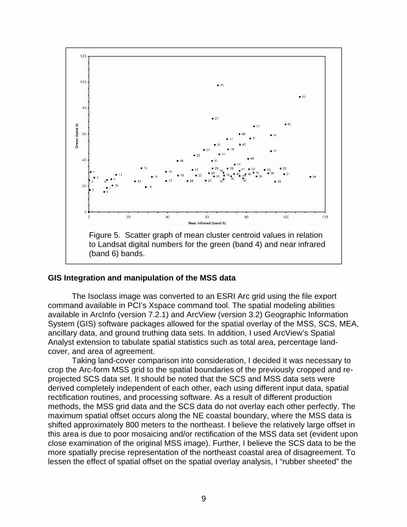
When assigning clusters to a land-cover category, I used the SCS data set, high altitude color infrared (CIR) aerial photographs, and my personal recollection of the area to group the 63 land-cover clusters into 8 land-cover categories (Table 4). Since my familiarity of the Seward Peninsula is confined to the areas around Council, the Kuzatrin River, and the roads connecting them, I gave these areas the most weight when assigning clusters to a certain land-cover category. As a visual guide for cluster assignments, I produced two scatter graphs of mean cluster centroid values for Landsat

8

bands 5 vs. 6 (Figure 4) and bands 4 vs. 6 (Figure 5). A land-cover category generally has closely grouped mean cluster values. The cluster to land-cover assignment crosswalk is illustrated in table 4.

Table 4. Isoclass cluster to land-cover assignments and associated pixel values for unsupervised classification of Seward Peninsula MSS image.

Landcover Class Short Name Pixel Value Cluster Numbers

Barrens Barrens 2 13,15,18,22,24,27,32,37,45,46,51,53,58

Dry Postrate Dwarf-shrub Tundra Dry Tundra 3 16,21,30,33,39,49,50,57

Moist Herbaceous Dwarf-shrub Tundra Moist Tundra 4 34,36,40,41,43,44, 48, 52,55,56

Wet Herbaceous Tundra Wet Tundra 5 17,19,23,29,38,42

Moist Low-shrub and Tall-Shrub Tundra Shrublands 7 26,28,31,47,54, 59, 60,61,64

Spruce Forest Spruce Forest 6 20,25,35 Water Water 1 2-12,14 Clouds and Snow Snow 8 62,63

Shadows Shadows 9 Derived from Water Clusters

Figure 4. Scatter graph of mean cluster centroid values in relation to Landsat digital numbers for the red (band 5) and near infrared (band 6) bands.

9

Figure 5. Scatter graph of mean cluster centroid values in relation to Landsat digital numbers for the green (band 4) and near infrared (band 6) bands.

GIS Integration and manipulation of the MSS data

The Isoclass image was converted to an ESRI Arc grid using the file export command available in PCI’s Xspace command tool. The spatial modeling abilities available in ArcInfo (version 7.2.1) and ArcView (version 3.2) Geographic Information System (GIS) software packages allowed for the spatial overlay of the MSS, SCS, MEA, ancillary data, and ground truthing data sets. In addition, I used ArcView’s Spatial Analyst extension to tabulate spatial statistics such as total area, percentage land-cover, and area of agreement.

Taking land-cover comparison into consideration, I decided it was necessary to crop the Arc-form MSS grid to the spatial boundaries of the previously cropped and re-projected SCS data set. It should be noted that the SCS and MSS data sets were derived completely independent of each other, each using different input data, spatial rectification routines, and processing software. As a result of different production methods, the MSS grid data and the SCS data do not overlay each other perfectly. The maximum spatial offset occurs along the NE coastal boundary, where the MSS data is shifted approximately 800 meters to the northeast. I believe the relatively large offset in this area is due to poor mosaicing and/or rectification of the MSS data set (evident upon close examination of the original MSS image). Further, I believe the SCS data to be the more spatially precise representation of the northeast coastal area of disagreement. To lessen the effect of spatial offset on the spatial overlay analysis, I “rubber sheeted” the

10

MSS data set to the SCS data set, using the Image Warp extension in Arc View. Rubber sheeting the MSS data set markedly reduced the spatial offset of the two data sets. Integration of Ancillary Data

The first version of the Isoclass image had several land-cover assignment problems that I attribute to similar spectral characteristics of land-cover categories, as well as poor radiometric correction of the original MSS mosaic. I made eight separate corrections to the original Isoclass-derived image.

A 300-meter digital elevation model (DEM) of Alaska (USGS, 1975) was used to reclassify areas of Dry Prostrate Dwarf-shrub Tundra to the Barrens land-cover category in areas with elevations lower than 100-meters. Additionally, areas of Wet Herbaceous Tundra higher than or equal to 300 meters were reclassified as Dry Prostrate Dwarf-shrub Tundra. This confusion between land-cover assignments is an example of similar spectral characteristics of land-cover classes, as well as errors resulting from poor radiometric correction of the original MSS mosaic. Before the DEM could be integrated, the 300-meter pixel size was resampled to 50-meter pixels, in order that the spatial resolution of the MSS data would not be compromised.

I made use of a variety of grid masks in areas that I felt were incorrectly classified. The first such mask was digitized over several large mountainous areas, converted to a grid, and used to reclassify water as shadows. Because of their low digital number value, shadows cast by hilly terrain or clouds are often misclassified as water. The other grid masks I used were based largely on the SCS data set. In these instances (as with the “water-to-shadow mask”), I simply digitized a polygon over an area where I wanted to change land-cover assignments, converted the polygon to a grid with a value of ten, and multiplied the MSS values by the mask grid value. Areas inside the polygon mask were multiplied by ten, and thus were easily recognizable in comparison to the unaltered MSS values outside of the mask. The multiplied values were then reclassified to their appropriate land-cover category. The following corrections (based largely on the SCS data set) were made to the MSS data set using this mask-multiply method:

• Moist Herbaceous Dwarf-shrub Tundra on mountaintops near the town of Council was reclassified as Dry Prostrate Dwarf-shrub Tundra. In addition, in the same mountain area, Wet Herbaceous Tundra was reclassified as Moist Low-shrub and Tall-shrub Tundra.

• Due to image stripping, a large number of pixels near the southeastern image border were incorrectly classified as Wet Herbaceous Tundra. They were reclassified as Spruce forest.

• Spruce forest pixels, which were outside of areas defined as Spruce Forest by the SCS data set, were reclassified as Moist Low-shrub and Tall-shrub Tundra.

• Two areas of fog in Imuruk Basin and offshore of the southwest coastal area were misclassified as Moist Low-shrub and Tall-shrub Tundra. These areas were reclassified as Water.

11

After corrections to the MSS land-cover classes had been made, the data were clipped to the spatial boundaries of the SCS data set. This was done to facilitate the comparison of the same geographic area (i.e. areas of offshore ocean water not included in the SCS data set (but present in the MSS data set) were excluded from comparison). The resulting image was used as the final comparison MSS data set. Comparison of the MSS, SCS, and MEA Data Sets

To quantitatively compare the data sets, I used both area-wise and spatial overlay comparisons. Using a cell size of 50-meters, the vector based MEA and SCS data were converted to raster based data, the identical form of the MSS data. Although the MSS data were clipped to the boundaries of the altered SCS data, the numbers of pixels in these two data sets are not exactly the same. This is due to the minor spatial offset of pixels in each data set; namely, pixels in the MSS data set slightly overlap the border of the SCS data set, but by no more than one pixel. Compared to the MSS data, the grid based MEA data has an even larger difference as to the total number of pixels contained in the data set. This is a result of the generalized nature of the original MEA data set, and the fact that I did not clip the MEA data to the SCS data set. The disparity between the number of pixels in each data set is not a significant factor affecting the land-cover categories in each data set.

The data for the area-wise comparison was calculated in terms of percentage of total area within a given land cover type. Two different area-wise comparisons were made. The first, comparing the SCS and MSS data (figure 6), and the second,

Figure 6. Area comparison of the classified MSS image with the seven class SCS dataset.

12

comparing the MEA, SCS and MSS data (figure 7). The MSS and SCS land-cover categories were simplified by combining the Barrens and Dry Tundra classes into an Alpine Tundra class in order to be compatible with the land-cover categories present in the MEA data set. Tables 1 and 2 illustrate the crosswalks that were used to simplify the MEA and SCS landcover classes for comparison to the MSS data

For the spatial overlay comparison, I generalized the MSS data in the same fashion as in the area-wise comparison, using the same land-cover crosswalk. Two difference matrices were produced: The first comparing the MEA and MSS data (table 5a), and the second, comparing the SCS and MSS data (table 5b). The difference matrices show the agreement between each land-cover category in each map. Values are in number of pixels contained in each land-cover category.

Figure 7. Area comparison of the classified MSS image with the six class SCS MEA datasets. Barrens, Dry Tundra, Snow and Shadow landcover classes were combined to create the Alpine Tundra class.

13

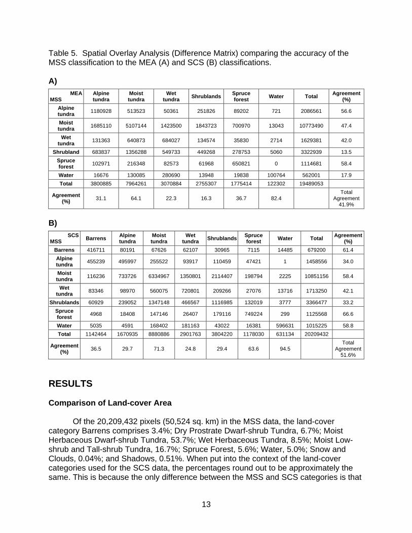
Table 5. Spatial Overlay Analysis (Difference Matrix) comparing the accuracy of the MSS classification to the MEA (A) and SCS (B) classifications. A)

MEA MSS

Alpine tundra

Moist tundra

Wet tundra Shrublands Spruce

forest Water Total Agreement (%)

Alpine tundra 1180928 513523 50361 251826 89202 721 2086561 56.6

Moist tundra 1685110 5107144 1423500 1843723 700970 13043 10773490 47.4

Wet tundra 131363 640873 684027 134574 35830 2714 1629381 42.0

Shrubland 683837 1356288 549733 449268 278753 5060 3322939 13.5 Spruce forest 102971 216348 82573 61968 650821 0 1114681 58.4

Water 16676 130085 280690 13948 19838 100764 562001 17.9 Total 3800885 7964261 3070884 2755307 1775414 122302 19489053

Agreement (%) 31.1 64.1 22.3 16.3 36.7 82.4

Total Agreement

41.9%

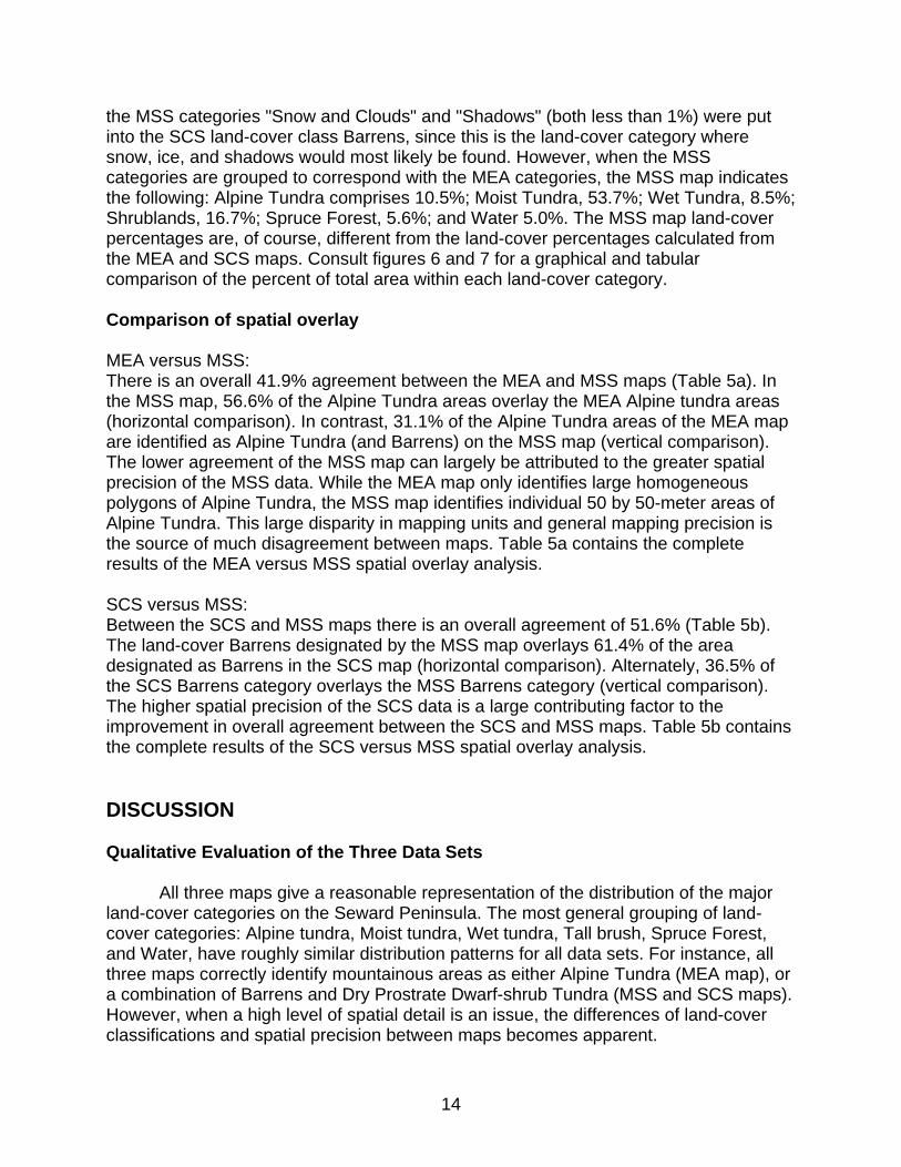
B)

SCS MSS Barrens Alpine

tundra Moist tundra

Wet tundra Shrublands Spruce

forest Water Total Agreement (%)

Barrens 416711 80191 67626 62107 30965 7115 14485 679200 61.4 Alpine tundra 455239 495997 255522 93917 110459 47421 1 1458556 34.0

Moist tundra 116236 733726 6334967 1350801 2114407 198794 2225 10851156 58.4

Wet tundra 83346 98970 560075 720801 209266 27076 13716 1713250 42.1

Shrublands 60929 239052 1347148 466567 1116985 132019 3777 3366477 33.2 Spruce forest 4968 18408 147146 26407 179116 749224 299 1125568 66.6

Water 5035 4591 168402 181163 43022 16381 596631 1015225 58.8 Total 1142464 1670935 8880886 2901763 3804220 1178030 631134 20209432

Agreement (%) 36.5 29.7 71.3 24.8 29.4 63.6 94.5

Total Agreement

51.6%

RESULTS Comparison of Land-cover Area

Of the 20,209,432 pixels (50,524 sq. km) in the MSS data, the land-cover category Barrens comprises 3.4%; Dry Prostrate Dwarf-shrub Tundra, 6.7%; Moist Herbaceous Dwarf-shrub Tundra, 53.7%; Wet Herbaceous Tundra, 8.5%; Moist Low-shrub and Tall-shrub Tundra, 16.7%; Spruce Forest, 5.6%; Water, 5.0%; Snow and Clouds, 0.04%; and Shadows, 0.51%. When put into the context of the land-cover categories used for the SCS data, the percentages round out to be approximately the same. This is because the only difference between the MSS and SCS categories is that

14

the MSS categories "Snow and Clouds" and "Shadows" (both less than 1%) were put into the SCS land-cover class Barrens, since this is the land-cover category where snow, ice, and shadows would most likely be found. However, when the MSS categories are grouped to correspond with the MEA categories, the MSS map indicates the following: Alpine Tundra comprises 10.5%; Moist Tundra, 53.7%; Wet Tundra, 8.5%; Shrublands, 16.7%; Spruce Forest, 5.6%; and Water 5.0%. The MSS map land-cover percentages are, of course, different from the land-cover percentages calculated from the MEA and SCS maps. Consult figures 6 and 7 for a graphical and tabular comparison of the percent of total area within each land-cover category. Comparison of spatial overlay MEA versus MSS: There is an overall 41.9% agreement between the MEA and MSS maps (Table 5a). In the MSS map, 56.6% of the Alpine Tundra areas overlay the MEA Alpine tundra areas (horizontal comparison). In contrast, 31.1% of the Alpine Tundra areas of the MEA map are identified as Alpine Tundra (and Barrens) on the MSS map (vertical comparison). The lower agreement of the MSS map can largely be attributed to the greater spatial precision of the MSS data. While the MEA map only identifies large homogeneous polygons of Alpine Tundra, the MSS map identifies individual 50 by 50-meter areas of Alpine Tundra. This large disparity in mapping units and general mapping precision is the source of much disagreement between maps. Table 5a contains the complete results of the MEA versus MSS spatial overlay analysis. SCS versus MSS: Between the SCS and MSS maps there is an overall agreement of 51.6% (Table 5b). The land-cover Barrens designated by the MSS map overlays 61.4% of the area designated as Barrens in the SCS map (horizontal comparison). Alternately, 36.5% of the SCS Barrens category overlays the MSS Barrens category (vertical comparison). The higher spatial precision of the SCS data is a large contributing factor to the improvement in overall agreement between the SCS and MSS maps. Table 5b contains the complete results of the SCS versus MSS spatial overlay analysis. DISCUSSION Qualitative Evaluation of the Three Data Sets

All three maps give a reasonable representation of the distribution of the major land-cover categories on the Seward Peninsula. The most general grouping of land-cover categories: Alpine tundra, Moist tundra, Wet tundra, Tall brush, Spruce Forest, and Water, have roughly similar distribution patterns for all data sets. For instance, all three maps correctly identify mountainous areas as either Alpine Tundra (MEA map), or a combination of Barrens and Dry Prostrate Dwarf-shrub Tundra (MSS and SCS maps). However, when a high level of spatial detail is an issue, the differences of land-cover classifications and spatial precision between maps becomes apparent.

15

The MEA map contains six land-cover classes (originally seven, Table 1), the SCS map has seven (originally 169, Table 2), and the MSS map, nine. In terms of land-cover classes, the original SCS map is unquestionably the most detailed representation. However, differentiating between 169 land-cover categories on a hard copy map is virtually impossible. If hard-copy production of a map is desirable, generalization of land-cover classes is a necessity. Cartographicaly speaking, it is best to keep the number of land-cover categories to a minimum, yet at the same time, it is important not to generalize categories to the point of having a map that does not effectively represent vegetation differences. Taking this into account, eight to ten land-cover categories is an appropriate number, six is too generalized, and 169 is far too complex.

Both the MEA and SCS maps were derived from a vector polygonal data set (i.e. they use polygons with coordinate referenced vertices to represent data). The vector approach is generally a more precise form of data, since the location of a point in space can be infinitely specified. In contrast, the MSS data is raster based (i.e. uses groups of 50 by 50-meter pixels to represent data). In the case of the MSS data set, spatial location can only be specified to within a 50-meter square polygon (pixel). Because of this, raster based data is generally less precise than vector data. However, when attempting to represent land-cover at small-scales (for example, a 1:1,000,000 scale), superior results are generally obtained by small-cell raster based data. This fact becomes apparent when you consider that the vector based SCS data has approximately 9,000 polygons of variable sizes. On the other hand, the MSS data has over 20 million polygons in the form of 50 by 50-meter pixels. Because vector data is limited to how many coordinates a human can enter into a computer, the digitally collected and processed MSS satellite data is able to show more spatial detail. For example, the SCS map indicates the presence of Moist Low-shrub and Tall-shrub Tundra, and Moist Herbaceous Dwarf-shrub tundra within mountain valleys - areas that were simply classed as Alpine Tundra by the MEA map. However, SCS polygons that represent areas of dominant Moist Low-shrub and Tall-shrub Tundra also commonly contain small areas of Moist Herbaceous Dwarf-shrub Tundra. While the SCS and MEA data sets do not give any sort of indication as to the heterogeneous nature of its vector polygons, this important information is provided by the MSS map on a pixel by pixel basis.

Overall, the MSS map shows more plant diversity in areas that were classed as only one land-cover type by the MEA and SCS maps. This fact is most apparent in areas that were categorized as Moist Tundra in the MEA map, and Moist Herbaceous Dwarf-shrub Tundra in the SCS map. The MSS map indicates that these areas also contain extensive areas of Moist Low-shrub and Tall-shrub Tundra (in addition to intermittent patches of Wet Herbaceous Tundra, Dry Prostrate Dwarf-shrub Tundra, and small bodies of standing water). The higher diversity of land-cover categories indicated by the MSS map is a significant improvement over the SCS and MEA maps. Major shortcomings of the three data sets

The MEA data set is by far the most generalized. It represents shoreline and vegetation boundaries as very linear and sharp-angled features, even at small scales. Additionally, no inland fresh water lakes, except one, are represented. This fact is the

16

largest reason why the “% area” of Water was so low on the MEA map (Figure 7). Future use of the MEA map should include the integration of a lakes and rivers map layer. The seven land-cover classes (reduced to six for map comparison) are too few, and the boundaries of which are of insufficient precision to warrant the use of the MEA map by any serious scientific research.

Land-cover classification and spatial detail of the SCS map is far superior to that of the MEA map. Similar to the MEA data, the complete lack of inland fresh water bodies is a curious drawback to a generally representative data set. Future use of the SCS map should include the integration of a lakes and rivers map layer. Although the SCS is the superior vector based data set, it gives no indication as to the diversity of land-cover types within its 9,000+ polygons. As stated before, 169 different land-cover designations are very difficult, if not impossible to differentiate on a printed hard-copy map. Therefore, simplification of the original land-cover categories is a necessity on a printed map.

The MSS-derived land-cover map has shortcomings as well. The effect of spectral mixing between mountain shadows, Barrens, and Dry Prostrate Dwarf-shrub Tundra categories often resulted in the classification of Wet herbaceous tundra, which in reality should be areas of either Barrens or Dry Prostrate Dwarf-shrub Tundra. Similarly, the sunny side of a hill typically gives off a different spectral reflectance than the shaded side of the same hill, even if the land-cover is entirely the same. As a result, some areas of the same land-cover type were classed differently, based upon hill aspect. This distortion caused by aspect is rectifiable by the integration of a digital elevation model (DEM), but in reality, would be very difficult to implement.

Poor radiometric correction is another consideration. In several instances, the seams between the individual MSS scenes are very apparent. This is a particular problem for an area to the west of the Kigluaik Mountain Range. The probable result is the partially incorrect land-cover classification of the immediate area surrounding the seam areas. Additionally, differences in the radiometric correction of the individual scenes has the potential to cause the same land-cover type to be misinterpreted as different land-cover categories in different scenes. Using the present mosaiced MSS data set, this problem cannot be solved, although corrections can be made using the mask- multiply method as outlined in “Integration of Ancillary Data” in the Methods section. Also, an area of low clouds and fog on the southwest coast of the Peninsula gives a false impression of Moist Low-shrub and Tall-shrub Tundra. Most of this error was corrected using the mask-multiply method. Additionally, a curious blob on the western edge of Imuruk Basin was also an area of concern. This blob could be a large mat of seaweed or perhaps a low cloud. Regardless of its composition, the blob area was reclassified as Water using the mask-multiply method. Despite its problems, the MSS data offers the most precise spatial representation of the distribution of vegetation on the Seward Peninsula. CONCLUSIONS 1) A raster-based remote sensing approach was an appropriate method of mapping the distribution of vegetation on the Seward Peninsula.

17

2) The MSS map provides a higher degree of spatial detail than the SCS and MEA vector-based maps. 3) The MSS map offers a better representation of the diversity of land-cover types within the individual SCS and MEA land-cover polygons. 4) Overall, percentages of each land-cover category are closely approximated by all three data sets (Figure 7). However, the precise distribution of the land-cover categories is highly variable, as indicated by the difference matrices (Table 5). 5) Areas of Moist Low-shrub and Tall-shrub Tundra that are not present on the SCS and MEA maps are identified on the MSS map. Since the MSS map indicates these areas occur in drainage-like patterns (associated with small intermittent streams), it is assumed that these shrubland areas do indeed exist. 6) Total agreement between the three maps is not impressive (41.9% between the MSS and MEA maps, and 51.6% between the MSS and SCS maps). The main cause of the relatively large margin of disagreement is most likely due to the comparison between vector based data (MEA and SCS) and raster based data (MSS). An additional factor affecting the low agreement of the maps could be caused by the independently derived land-cover classification systems employed by the creators of each data set, as well inter-scene radiometric correction problems. 7) The MSS map offers possibly the first Multi-Spectral Sensor-derived land-cover map of the entire Seward Peninsula. An accuracy assessment of MSS map is planned for the near future.

18

ACKNOWLEGEMENTS

This research study was funded through the Research Experience for Undergraduates (REU) program, sponsored by the National Science Foundation. MSS satellite imagery was provided by the USGS, EROS Alaska Field Office in Anchorage, AK. Special thanks to Skip Walker, Tako Reynolds, Amber Moody, David Wallin, David Wirth, Carl Markon and especially Hilmar Maier for their guidance and suggestions throughout the development of this research project. LITERATURE CITED Campbell, J.B. 1996. Introduction to Remote Sensing. New York: The Guilford Press. Joint Federal State Land Use Planning Commission. 1973. Major Ecosystems of

Alaska Map. (http://agdc.usgs.gov/data/usgs/erosafo/ecosys/metadata/ecosys.html).

Robinson, A.H., Morrison, J.L., Muehrcke, P.C, et al. 1995. Elements of Cartography.

New York: John Wiley and Sons. Rowntree, P.R. 1997. Global and regional patterns of climate change: recent

predictions for the arctic. Global Change and Arctic Terrestrial Ecosystems. pp. 82-109.

Spetzman, L.A. 1959. Vegetation of Alaska. Professional Paper 302-B. USGS.

Washington D.C. USDA, Soil Conservation Service. 1985. Range Survey of the Seward Peninsula

Reindeer Ranges, Alaska. (http://www.ak.nrcs.usda.gov/technical/metadata/veg_site.html).

USGS, EROS Alaska Field Office. 1997. Alaska 300m digital elevation model.

(http://agdc.usgs.gov/data/usgs/erosafo/300m/dem/metadata/dem300m.html) Walker, D.A., 1995, Towards a new Arctic Vegetation Map: St. Petersburg Workshop.

Arctic and Alpine Research. 27(1):103-104.

19

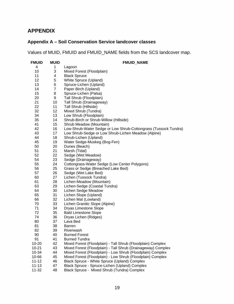
APPENDIX Appendix A – Soil Conservation Service landcover classes Values of MUID, FMUID and FMUID_NAME fields from the SCS landcover map.

FMUID MUID FMUID_NAME 4 1 Lagoon

10 3 Mixed Forest (Floodplain) 11 4 Black Spruce 12 5 White Spruce (Upland) 13 6 Spruce-Lichen (Upland) 14 7 Paper Birch (Upland) 15 8 Spruce-Lichen (Palsa) 20 9 Tall Shrub (Floodplain) 21 10 Tall Shrub (Drainageway) 22 11 Tall Shrub (Hillside) 32 12 Mixed Shrub (Tundra) 34 13 Low Shrub (Floodplain) 35 14 Shrub-Birch or Shrub-Willow (Hillside) 41 15 Shrub Meadow (Mountain) 42 16 Low-Shrub-Water Sedge or Low Shrub-Cottongrass (Tussock Tundra) 43 17 Low Shrub-Sedge or Low Shrub-Lichen Meadow (Alpine) 44 18 Shrub-Lichen (Upland) 45 19 Water Sedge-Muskeg (Bog-Fen) 50 20 Dunes (Beach) 51 21 Marsh (Tidal) 52 22 Sedge (Wet Meadow) 54 23 Sedge (Drainageway) 55 24 Cottongrass-Water Sedge (Low Center Polygons) 56 25 Grass or Sedge (Breached Lake Bed) 57 26 Sedge (Wet Lake Bed) 60 27 Lichen (Tussock Tundra) 61 28 Lichen-Meadow (Mountain) 63 29 Lichen-Sedge (Coastal Tundra) 64 30 Lichen Sedge Meadow 65 31 Lichen Slope (Upland) 66 32 Lichen Mat (Lowland) 70 33 Lichen Granitic Slope (Alpine) 71 34 Dryas Limestone Slope 72 35 Bald Limestone Slope 74 36 Dryas Lichen (Ridges) 80 37 Lava Bed 81 38 Barren 82 39 Riverwash 90 40 Burned Forest 91 41 Burned Tundra

10-20 42 Mixed Forest (Floodplain) - Tall Shrub (Floodplain) Complex 10-21 43 Mixed Forest (Floodplain) - Tall Shrub (Drainageway) Complex 10-34 44 Mixed Forest (Floodplain) - Low Shrub (Floodplain) Complex 10-66 45 Mixed Forest (Floodplain) - Low Shrub (Floodplain) Complex 11-12 46 Black Spruce - White Spruce (Upland) Complex 11-13 47 Black Spruce - Spruce-Lichen (Upland) Complex 11-32 48 Black Spruce - Mixed Shrub (Tundra) Complex

20

FMUID MUID FMUID_NAME 11-44 49 Black Spruce - Shrub-Lichen (Upland) Complex 11-45 50 Black Spruce - Water Sedge-Muskeg (Bog-Fen) Complex 11-60 51 Black Spruce - Lichen (Tussock Tundra) Complex 12-13 52 White Spruce (Upland) - Spruce-Lichen (Upland) Complex 12-14 53 White Spruce (Upland) - Paper Birch (Upland) Complex 12-22 54 White Spruce (Upland) - Tall Shrub (Hillside) Complex 12-32 55 White Spruce (Upland) - Mixed Shrub (Tundra) Complex 12-44 56 White Spruce (Upland) - Shrub-Lichen (Upland) Complex 12-60 57 White Spruce (Upland) - Lichen (Tussock Tundra) Complex 13-11 58 Spruce-Lichen (Upland) - Shrub-Lichen (Upland) Complex 13-44 59 Spruce-Lichen (Upland) - Shrub-Lichen (Upland) Complex 15-45 60 Spruce-Lichen (Palsa) - Water Sedge-Muskeg (Bog-Fen) Complex 20-34 61 Tall Shrub (Floodplain) - Low Shrub (Floodplain) Complex 20-54 62 Tall Shrub (Floodplain) - Sedge (Drainageway) Complex 20-82 63 Tall Shrub (Floodplain) - Riverwash Complex 21-13 64 Tall Shrub (Drainageway) - Spruce-Lichen (Upland) Complex 21-32 65 Tall Shrub (Drainageway) - Mixed Shrub (Tundra) Complex 21-34 66 Tall Shrub (Drainageway) - Low Shrub (Floodplain) Complex 21-35 67 Tall Shrub (Drainageway) - Shrub-Birch or Shrub-Willow (Hillside) Complex

21-42 68 Tall Shrub (Drainageway) - Low Shrub-Water Sedge or Low Shrub-Cottongrass (Tussock Tundra) Complex

21-60 69 Tall Shrub (Drainageway) - Lichen (Tussock Tundra) Complex 22-12 70 Tall Shrub (Hillside) - White Spruce (Upland) Complex 22-32 71 Tall Shrub (Hillside) - Mixed Shrub (Tundra) Complex 22-41 72 Tall Shrub (Hillside) - Shrub Meadow (Mountain) Complex

22-42 73 Tall Shrub (Hillside) - Low Shrub-Water Sedge or Low Shrub-Cottongrass (Tussock Tundra) Complex

22-52 74 Tall Shrub (Hilside) - Sedge (Wet Meadow) Complex 22-61 75 Tall Shrub (Hillside) - Lichen Meadow (Mountain) Complex 22-65 76 Tall Shrub (Hillside) - Lichen Slope (Upland) Complex

32-42 77 Mixed Shrub (Tundra) - Low Shrub-Water Sedge or Low Shrub-Cottongrass (Tussock Tundra) Complex

32-44 78 Mixed Shrub (Tundra) - Shrub-Licehn (Upland) Complex 32-52 79 Mixed Shrub (Tundra) - Sedge (Wet Meadow) Complex 32-54 80 Mixed Shrub (Tundra) - Sedge (Drainageway) Complex 32-60 81 Mixed Shrub (Tundra) - Lichen (Tussock Tundra) Complex

34-42 82 Low Shrub (Floodplain) - Low Shrub-Water Sedge or Low Shrub-Cottongrass (Tussock Tundra) Complex

34-51 83 Low Shrub (Floodplain) - Marsh (Tidal) Complex 34-54 84 Low Shrub (Floodplain) - Sedge (Drainageway) Complex

34-55 85 Low Shrub (Floodplain) - Cottongrass-Water Sedge (Low Center Polygons) Complex

34-56 86 Low Shrub (Floodplain) - Grass or Sedge (Breached Lake Bed) Complex 34-82 87 Low Shrub (Floodplain) - Riverwash Complex 35-12 88 Shrub-Birch or Shrub Willow (Hillside) - White Spruce (Upland) Complex 35-41 89 Shrub-Birch or Shrub-Willow (Hillside) - Shrub (Mountain) Complex

35-43 90 Shrub-Birch or Shrub-Willow (Hillside) - Low Shrub Sedge or Low Shrub Lichen Meadow (Alpine) Complex

35-52 91 Shrub-Birch or Shrub-Willow (Hillside) - Sedge (Wet Meadow) Complex 35-61 92 Shrub-Birch or Shrub-Willow (Hillside) - Lichen Meadow (Mountain) Complex 41-20 93 Shrub Meadow (Mountain) - Tall Shrub (Floodplain) Complex 41-32 94 Shrub Meadow (Mountain) - Mixed Shrub (Tundra) Complex

41-42 95 Shrub Meadow (Mountain) - Low Shrub-Water Sedge or Low Shrub-Cottongrass (Tussock Tundra) Complex

41-43 96 Shrub Meadow (Mountain) - Low Shrub-Sedge or Low Shrub-Lichen Meadow

21

FMUID MUID FMUID_NAME (Alpine) Complex

41-52 97 Shrub Meadow (Mountain) - Sedge (Wet Meadow) Complex 41-54 98 Shrub Meadow (Mountain) - Sedge (Drainageway) Complex 41-56 99 Shrub Meadow (Mountain) - Grass or Sedge (Breached Lake Bed) Complex 41-61 100 Shrub Meadow (Mountain) - Lichen Meadow (Mountain) Complex 41-80 101 Shrub Meadow (Mountain) - Lava Bed Complex

42-34 102 Low Shrub-Water Sedge or Low Shrub-Cottongrass (Tussock Tundra) - Low Shrub (Floodplain) Complex

42-43 103 Low Shrub-Water Sedge or Low Shrub-Cottongrass (Tussock Tundra) - Low Shrub-Sedge or Lichen Meadow (Alpine) Complex

42-44 104 Low Shrub-Water Sedge or Low Shrub-Cottongrass (Tussock Tundra) - Shrub-Lichen (Upland) Complex

44-52 105 Shrub-Lichen (Upland) - Sedge (Wet Meadow) Complex

42-54 106 Low Shrub-Water Sedge or Low Shrub-Cottongrass (Tussock Tundra) - Sedge (Drainageway) Complex

42-55 107 Low Shrub-Water Sedge or Low Shrub-Cottongrass (Tussock Tundra) - Cottongrass-Water Sedge (Low Center Polygons) Complex

42-56 108 Low Shrub-Water Sedge or Low Shrub-Cottongrass (Tussock Tundra) - Grass or Sedge (Breached Lake Bed) Complex

42-57 109 Low Shrub-Water Sedge or Low Shrub-Cottongrass (Tussock Tundra) - Sedge (Wet Lake Bed) Complex

42-60 110 Low Shrub-Water Sedge or Low Shrub-Cottongrass (Tussock Tundra) - Lichen (Tussock Tundra) Complex

42-80 111 Low Shrub-Water Sedge or Low Shrub-Cottongrass (Tussock Tundra) - Lava Bed Complex

43-21 112 Low Shrub-Sedge or Low Shrub-Lichen Meadow (Alpine) - Tall Shrub (Drainageway) Complex

43-22 113 Low Shrub-Sedge or Low Shrub-Lichen Meadow (Alpine) - Tall Shrub (Hillside) Complex

43-32 114 Low Shrub-Sedge or Low Shrub-Lichen Meadow (Alpine) - Mixed Shrub (Tundra) Complex

43-35 115 Low Shrub-Sedge or Low Shrub-Lichen Meadow (Alpine) - Shrub-Birch or Shrub-Willow (Hillside) Complex

43-52 116 Low Shrub-Sedge or Low Shrub-Lichen Meadow (Alpine) - Sedge (Wet Meadow) Complex

43-55 117 Low Shrub-Sedge or Low Shrub-Lichen Meadow (Alpine) - Cottongrass-Water Sedge (Low Center Polygons) Complex

43-71 118 Low Shrub-Sedge or Low Shrub-Lichen Meadow (Alpine) - Dryas Limesotne Slope Complex

44-22 119 Shrub-Lichen (Upland) - Tall Shrub (Hillside) Complex 44-72 120 Shrub-Lichen (Upland) - Bald Limestone Slope Complex 50-52 121 Dunes (Beach) - Sedge (Wet Meadow) Complex 51-52 122 Marsh (Tidal) - Sedge (Wet Meadow) Complex 52-32 123 Sedge (Wet Meadow) - Mixed Shrub (Tundra) Complex 52-34 124 Sedge (Wet Meadow) - Low Shrub (Floodplain) Complex 52-35 125 Sedge (Wet Meadow) - Shrub-Birch or Shrub-Willow (Hillside) Complex 52-41 126 Sedge (Wet Meadow) - Shrub Meadow (Mountain) Complex

52-43 127 Sedge (Wet Meadow) - Low Shrub-Sedge or Low Shrub-Lichen Meadow (Alpine) Complex

52-54 128 Sedge (Wet Meadow) - Sedge (Drainageway) Complex 52-55 129 Sedge (Wet Meadow) - Cottongrass-Water Sedge (Low Center Polygons) Complex52-56 130 Sedge (Wet Meadow) - Grass or Sedge (Breach Lake Bed) Complex 52-60 131 Sedge (Wet Meadow) - Lichen (Tussock Tundra) Complex 52-61 132 Sedge (Wet Meadow) - Lichen Meadow (Mountain) Complex 52-72 133 Sedge (Wet Meadow) - Bald Limestone Slope Complex

22

FMUID MUID FMUID_NAME 55-42 134 Cottongrass-Water Sedge (Low Center Polygons) - Low Shrub-Sedge or Low-

Shrub-Cottongrass (Tussock Tundra) Complex 55-57 135 Cottongrass-Water Sedge (Low Center Polygons) - Sedge (Wet Lake Bed) Complex

56-55 136 Grass or Sedge (Breached Lake Bed) - Cottongrass-Water Sedge (Low Center Polygons) Complex

56-57 137 Grass or Sedge (Breached Lake Bed) - Sedge (Wet Lake Bed) Complex 57-34 138 Sedge (Wet Lake Bed) - Low Shrub (Floodplain) Complex 60-20 139 Lichen (Tussock Tundra) - Tall Shrub (Floodplain) Complex 60-32 140 Lichen (Tussock Tundra) - Mixed Shrub (Tundra) Complex 60-34 141 Lichen (Tussock Tundra) - Low Shrub (Floodplain) Complex

60-42 142 Lichen (Tussock Tundra) - Low Shrub-Water Sedge or Low Shrub Cottongrass (Tussock Tundra) Complex

60-54 143 Lichen (Tussock Tundra) - Sedge (Drainageway) Complex

60-55 144 Lichen (Tussock Tundra) - Cottongrass-Water Sedge (Low Center Polygons) Complex

60-56 145 Lichen (Tussock Tundra) - Grass or Sedge (Breached Lake Bed) Complex 60-80 146 Lichen (Tussock Tundra) - Lava Bed Complex 61-32 147 Lichen Meadow (Mountain) - Mixed Shrub (Tundra) Complex

61-43 148 Lichen Meadow (Mountain) - Low Shrub-Sedge or Low Shrub-Lichen Meadow (Alpine) Complex

61-44 149 Lichen Meadow (Mountain) - Shrub-Lichen (Upland) Complex 61-52 150 Lichen Meadow (Mountain) - Sedge (Wet Meadow) Complex 61-64 151 Lichen Meadow (Mountain) - Lichen-Sedge Meadow Complex 61-72 152 Lichen Meadow (Mountain) - Bald Limestone Slope Complex 61-74 153 Lichen Meadow (Mountain) - Dryas-Lichen (Ridges) Complex

63-43 154 Lichen-Sedge (Coastal Tundra) - Low Shrub-Sedge or Low Shrub-Lichen Meadow (Alpine) Complex

63-52 155 Lichen-Sedge (Coastal Tundra) - Sedge (Wet Meadow) Complex 63-54 156 Lichen-Sedge (Coastal Tundra) - Sedge (Drainageway) Complex

64-43 157 Lichen Sedge Meadow - Low Shrub-Sedge or Low Shrub-Lichen Meadow (Alpine) Complex

66-20 158 Lichen Mat (Lowland) - Tall Shrub (Drainageway) Complex 66-54 159 Lichen Mat (Lowland) - Sedge (Drainageway) Complex 66-55 160 Lichen Mat (Lowland) - Cottongrass-Water Sedge (Low Center Polygons) Complex 70-41 161 Lichen Granitic Slope (Alpine) - Lichen Meadow (Mountain) Complex 70-43 162 Lichen Granitic Slope (Alpine) - Lichen Meadow (Mountain) Complex 70-61 163 Lichen Granitic Slope (Alpine) - Lichen Meadow (Mountain) Complex 71-52 164 Dryas Limestone Slope - Sedge (Wet Meadow) Complex 72-12 165 Bald Limestone Slope - White Spruce (Upland) Complex 72-22 166 Bald Limestone Slope - Tall Shrub (Hillside) Complex 80-60 167 Lava Bed - Lichen (Tussock Tundra) 90-22 168 Burned Forest - Tall Shrub (Hillside) Complex