A Preference-based Evolutionary Algorithm forMultiobjective Optimization

L. Thiele thiele@tik.ee.ethz.chETH-Zurich, Department of Information Technology and Electrical Engineering,Gloriastrasse 35, CH-8092 Zurich, Switzerland

K. Miettinen kaisa.miettinen@jyu.fiDepartment of Mathematical Information Technology, P.O. Box 35 (Agora), FI-40014University of Jyvaskyla, Finland

P. J. Korhonen pekka.korhonen@hse.fiHelsinki School of Economics, Department of Business Technology, P.O. Box 1210,FI-00101 Helsinki, Finland

J. Molina julian.molina@uma.esDepartment of Applied Economics, University of Malaga, E-29071 Malaga, Spain

AbstractIn this paper, we discuss the idea of incorporating preference information into evolu-tionary multiobjective optimization and propose a preference-based evolutionary ap-proach that can be used as an integral part of an interactive algorithm. One algorithmis proposed in the paper. At each iteration, the decision maker is asked to give prefer-ence information in terms of her/his reference point consisting of desirable aspirationlevels for objective functions. The information is used in an evolutionary algorithmto generate a new population by combining the fitness function and an achievementscalarizing function. In multiobjective optimization, achievement scalarizing functionsare widely used to project a given reference point into the Pareto optimal set. In ourapproach, the next population is thus more concentrated in the area where more pre-ferred alternatives are assumed to lie and the whole Pareto optimal set does not haveto be generated with equal accuracy. The approach is demonstrated by numerical ex-amples.

KeywordsMultiple objectives, multiple criteria decision making, preference information, refer-ence point, achievement scalarizing function, Pareto optimality, fitness evaluation.

1 Introduction

Most real-life decision and planning situations involve multiple conflicting criteriathat should be considered simultaneously. The term multiple criteria decision making(MCDM) or multiobjective optimization refers to solving such problems. For them, it ischaracteristic that no unique solution exists but a set of mathematically equally goodsolutions can be identified. These solutions are known as efficient, nondominated, non-inferior or Pareto optimal solutions. In the MCDM literature, the terms are often seenas synonyms.

In the MCDM literature, the idea of solving a multiobjective optimization problemis understood as helping a human decision maker (DM) to consider the multiple crite-ria simultaneously and to find a Pareto optimal solution that pleases him/her most.

Thus, the solution process always requires the involvement of the DM and the finalsolution is determined by her/his preferences. Usually, decision support systems op-erate iteratively generating Pareto optimal solutions based on some rules and the DMmakes choices and specifies preference information. Those choices are used to lead thealgorithm to generate more Pareto optimal solutions until the DM reaches the most sat-isfactory, that is, the final solution. In other words, not all Pareto optimal solutions aregenerated but only the ones the DM finds interesting.

On the other hand, evolutionary multiobjective optimization (EMO) methods takea different approach to solving multiobjective optimization problems. It is also im-portant to note that when compared to the MCDM literature, there is a difference interminology. EMO approaches generate a set of nondominated solutions which is arepresentation approximating the (unknown) Pareto optimal set. Thus in EMO, Paretooptimality and nondominance are not synonyms. The intervention of the DM is notneeded in the process. So far, rather little interest has been paid in the literature tochoosing one of the nondominated solutions as the final one. However, there is typi-cally a need to identify such a solution indicating which values the decision variablesshould have in order to get the best possible values for the conflicting criteria. The dif-ficulty of identifying the best nondominated solutions is even more evident when thereare more than two criteria and it, thus, is difficult to display the set of nondominatedsolutions.

One can say that MCDM and EMO approaches are based on different philosophieseven though they are applied to similar problems. In this paper, we combine elementsof solution techniques used in MCDM and EMO communities and suggest a way tohybridize them. Because it seems that publications in the literature have mostly con-centrated on either MCDM or EMO approaches, we also wish to describe some MCDMdevelopments to those more familiar with EMO approaches.

Helping DMs in solving multiobjective optimization problems has been the sub-ject of intensive studies since the beginning of the 1970’s (see, e.g., Benayoun et al.1971, Geoffrion et al. 1972 and Zionts and Wallenius 1976). However, many theoreticalconcepts were defined much earlier (see, e.g., Koopmans 1971, Kuhn and Tucker 1951and Pareto 1906) and, actually, many ideas originated from the theory of mathematicalprogramming.

Surveys of methods developed for multiobjective optimization problems includeChankong and Haimes (1983), Hwang and Masud (1979), Miettinen (1999), Sawaragi etal. (1985) and Steuer (1986). For example, in Hwang and Masud (1979) and Miettinen(1999), multiobjective optimization methods are classified into four classes accordingto the role of the DM in the solution process. Sometimes, there is no DM available andin this case some neutral compromise solution is to be identified. Such no-preferencemethods must be used if no preference information is available. In a priori methods, theDM articulates preference information and one’s hopes before the solution process. Thedifficulty here is that the DM does not necessarily know the limitations and possibil-ities of the problem and may have too optimistic or pessimistic hopes. Alternatively,a set of Pareto optimal solutions can be generated first and then the DM is supposedto select the most preferred one among them. Typically, evolutionary multiobjectiveoptimization algorithms belong to this class of a posteriori methods. If there are morethan two criteria in the problem, it may be difficult for the DM to analyze the largeamount of information and, on the other hand, generating the set of Pareto optimal ornondominated alternatives may be computationally expensive.

The drawbacks of both a priori and a posteriori methods can be overcome if there is

2

a DM available who is willing to participate in the solution process and direct it accord-ing to her/his preferences. So-called interactive methods form a solution pattern which isiteratively repeated as long as the DM wants. After each iteration, the DM is providedwith one or some Pareto optimal solutions that obey the preferences expressed as wellas possible and (s)he can specify more preference information. This can be, for exam-ple, in the form of trade-offs, pairwise comparisons, aspiration levels, classification ofobjective functions, etc. The responses are used to generate presumably improved solu-tions. In this way, the DM can learn about the problem and fine-tune one’s preferencesif needed. The ultimate goal is to find the solution that satisfies her/him most. In-teractive methods are computationally inexpensive because only such Pareto optimalsolutions are generated that are interesting to the DM. In order to support the DM bet-ter, the ideas of interactive and a posteriori methods can also be hybridized to utilizeadvantages of both the approaches see, for example, Klamroth and Miettinen (2008).

Besides using different types of preference information, interactive methods alsodiffer from each other in the way the information is utilized in generating new, im-proved solutions and what is assumed about the behaviour of the DM. Typically, dif-ferent methods convert the original multiple objectives as well as the preference in-formation into an optimization problem with a single objective function using a so-called scalarizing function. The resulting problem is then solved with some appropri-ate single objective solver. When dealing with real-life problems, there may be integer-valued variables or nonconvex or nondifferentiable functions involved, which set re-quirements on the solvers used.

As discussed above, including DM’s preferences is important when dealing withmultiobjective optimization problems, as the aim is to help the DM to find the mostpreferred solutions without exploring the whole set of Pareto optimal solutions andlead her/him to a better knowledge of the problem being solved. However, the num-ber of EMO methods including DM’s preferences is relatively small in contrast to thenumber of interactive approaches found in the MCDM literature. Only some works canbe found combining EMO algorithms and interactive methods, although many authorshave been asking for such approaches, including Hanne (2006).

Coello (2000) has presented a survey on including preferences when using a mul-tiobjective evolutionary method: Fonseca and Fleming (1993) probably suggested theearliest attempt to incorporate preferences, and the proposal was to use MOGA to-gether with goal information as an additional criterion to assign ranks to the membersof a population. Greenwood et al. (1997) used value functions to perform the rankingof attributes, and also incorporated preference information into the survival criteria.Cvetkovic and Parmee (1999, 2002) and Parmee et al. (2000) used binary preferencerelations (translated into weights) to narrow the search. These weights were used insome different ways to modify the concept of dominance. Rekiek et al. (2000) usedthe PROMETHEE method (a multiattribute decision analysis method for discrete al-ternatives) to generate weights for an EMO method. On the other hand, Massebeufet al. (1999) used PROMETHEE II in an a posteriori form: an EMO algorithm gener-ated nondominated solutions and PROMETHEE II selected some of them based on theDM’s preferences. Deb (1999a) used variations of compromise programming to bias thesearch of an EMO approach. Finally, in Deb (1999b) the DM was required to providegoals for each objective.

More recently, some other approaches have been published. Phelps and Koksalan(2003) used pairwise comparisons to include DM’s preferences in the fitness function.In the guided multi-objective evolutionary algorithm (G-MOEA) proposed by Branke

3

et al. (2001) user preferences were taken into account using trade-offs, supplied by theDM, to modify the definition of dominance. In Branke and Deb (2004), two schemeswere proposed to include preference information when using an EMO (they used theNSGA-II for testing): modifying the definition of dominance (using the guided domi-nance principle of G-MOEA) and using a biased crowding distance based on weights.

Sakawa and Kato (2002) used reference points in a traditional approach. One ref-erence point was used to compute a single tentative efficient solution, and at each itera-tion, the DM was asked to specify a new reference point until satisfaction was reached.Instead of using classical (crisp) reference points, they use a fuzzy approach to repre-sent the DM’s preferences. The main contribution of this paper is (besides the coding-decoding method to represent solutions) the way preferences are represented in a fuzzyway.

Finally, in Deb et al. (2005), preferences were included through the use of refer-ence points. Also a guided dominance scheme and a biased crowding scheme weresuggested. Deb et al. (2005) are using the concept of the reference point but do notapply an achievement scalarizing function, which is an essential concept in the con-text of reference points, as suggested by Wierzbicki (1980). An achievement scalarizingfunction is a ”tool” which guarantees that the point found by means of the scalarizingfunction is Pareto optimal. In addition, an achievement scalarizing function enablesfinding a solution which satisfies the preferences the DM has specified in the referencepoint. The main difference of our approach when compared to the one proposed byDeb et al. (2005), as will be shown later, is that we directly use reference point informa-tion in fitness evaluation (through an achievement scalarizing function that will alsobe defined later) in an indicator-based evolutionary algorithm IBEA (see, Zitzler andKuenzli, 2004).

In this paper, we suggest a hybrid approach where we combine ideas from bothevolutionary and interactive multiobjective optimization (as encouraged e.g. in Brankeet al. (2008)). The principle is to incorporate preference information coming from aDM in the evolutionary approach. As justified earlier in this section, we are not inter-ested in approximating the whole Pareto optimal set. Instead, we first give a roughapproximation, and then generate a more accurate approximation of the area wherethe DM’s most satisfactory solution lies. In practice, the DM is asked to give prefer-ence information in terms of her/his reference point consisting of desirable aspirationlevels for objective functions. This information is used in a preference-based evolu-tionary algorithm that generates a new population by combining the fitness functionand a so-called achievement scalarizing function containing the reference point. Thenext population is more concentrated in the area where more preferred alternatives areassumed to lie. With the new evolutionary approach, the DM can direct the search to-wards the most satisfactory solution but still learn about the behaviour of the problem,which enables her/him to adjust one’s preferences. It is easier to specify the referencepoint after the DM has seen a rough approximation of Pareto optimal solutions avail-able but the approximation only has to be improved in quality in the interesting partsof the Pareto optimal set. Because evolutionary algorithms set no assumptions on thedifferentiability, convexity or continuity of the functions involved, the approach can beused in solving complicated real-life problems.

In summary, the suggested approach has two main new elements: first an achieve-ment scalarizing function is adapted for an EMO algorithm and, in particular, fitnessevaluation in it, and secondly an interactive solution method is proposed which isbased on utilizing this achievement scalarization function in evolutionary optimiza-

4

tion. In this way, we modify the traditional aim of EMO algorithms (in generating anapproximation of the whole Pareto optimal set) and incorporate ideas (used in MCDMmethods) of decision support. Multiobjective optimization is more than biobjective op-timization. Thus, the motivation is to create new methods that can conveniently beused when the problem to be solved has more than two criteria and when applyingplain EMO ideas is not efficient.

The rest of this paper is organized as follows. In Section 2, we introduce the basicconcepts and notations of multiobjective optimization. Section 3 is devoted to discus-sion on different ways of handling preference information. We pay special attention toreference point based methods and achievement scalarizing functions. We introduceour preference based interactive algorithm in Section 4 and demonstrate how it workswith a few examples in Section 5. Finally, we draw some conclusions in Section 6.

2 Multiobjective optimization

A multiobjective optimization problem can be written in the form

minimize f(x) = (f1(x), . . . , fk(x))

subject to x ∈ X,(1)

where X ⊂ Rn is a feasible set of decision variables and f : R

n → Rk. The n-

dimensional space Rn is called a variable space and the functions fi, i = 1, . . . , k, are

objective functions or criteria. The k-dimensional space Rk is a so-called criterion space

and its subset, the image of the feasible set, called a feasible criterion region, can now bewritten as Q = {q|q = f(x), x ∈ X}. The set Q is of special interest and most consider-ations in multiobjective optimization are made in the criterion space.

Problem (1) has several mathematically equivalent solutions. They are called ef-ficient, nondominated, noninferior or Pareto optimal (sometimes in the MCDM litera-ture some of these concepts are associated with decision and the others with criterionspaces). Any choice from among the set of Pareto optimal solutions is impossible, un-less we have additional information available about the DM’s preference structure. Tobe more specific, we have the following definitions:

Definition 1 In (1), a vector f(x), x ∈ X , is said to dominate another vector f(y), y ∈ X , iffi(x) ≤ fi(y) for all i = 1, . . . , k, and the inequality is strict for at least one i.

Definition 2 In (1), a vector f(x∗), x∗ ∈ X , is nondominated if there does not exist anotherx ∈ X such that f(x) dominates f(x∗).

The set of all nondominated solutions is called the nondominated frontier or Paretooptimal set. The final (“best”) solution of problem (1) is called the most preferred solution.It is a nondominated solution preferred by the DM to all other solutions. We also willuse the concept of weakly nondominated solutions which is defined by replacing allinequalities by strict inequalities in Definition 1. The set of nondominated solutions isa subset of weakly nondominated solutions.

3 On preference information in different MCDM methods

Several dozens of methods have been developed during the last over 30 years toaddress multiobjective optimization problems see, for example, the textbooks byChankong and Haimes (1983), Hwang and Masud (1979), Miettinen (1999), Sawaragiet al. (1985) and Steuer (1986). Typically, they always require the intervention of a DMat some stage in the solution process. A popular way to involve the DM in the solution

5

process is to use interactive approaches as discussed in the introduction. Because thegoal is to support the DM, we can refer to the tools used as decision support systems.The ultimate goal is to find the most preferred solution of the DM.

There is no single criterion for evaluating multiple criteria decision support sys-tems. Instead, several relevant criteria can be introduced, for example:

• the system recognizes and generates Pareto optimal solutions and helps the DM toget a “holistic” view of the Pareto optimal set;

• the system helps the DM feel convinced that the final solution is the most preferredone, or at least close enough to that;

• the system provides an intuitive user interface and does not require too much timefrom the DM to find the final solution.

Provided that the problem is correctly specified, the final solution of a rational DMis always Pareto optimal. Therefore, it is important that the system is able to recognizeand generate Pareto optimal solutions. No system can provide a DM with a capabil-ity to compare all alternatives simultaneously. However, a good system can providea holistic view over the alternatives and assist the DM in becoming convinced thather/his final choice is the best or at least close to the best solution. The user interfaceplays an important role in that aspect.

3.1 Overview of some interactive methods

An example of early interactive methods is the GDF method, see Geoffrion et al. (1972).It assumes that there exists an unknown value function that represents the preferencesof the DM and (s)he wants to maximize this function. Even though the function is notexplicitly known, information about it is asked from the DM in the form of responsesto specific questions involving marginal rates of substitution of pairs of objective func-tions and, in this way, the DM guides the solution process towards the most preferredsolution. This approach assumes consistency on the DM’s part as well as some differ-entiability assumptions.

Alternatively, a small sample of Pareto optimal solutions can be generated and theDM is supposed to select the most preferred one of them. Then, the next sample ofPareto optimal solutions is generated so that it concentrates on the neighbourhood ofthe selected one, see Steuer (1986).

It has been shown in Larichev (1992) that for a DM, classification of objective func-tions is a cognitively valid way of expressing preference information. Classificationmeans that the objective function values at the current Pareto optimal solution areshown to the DM and the DM is asked to indicate how the solution should be improvedby classifying the functions according to whether their current values are acceptable,should be improved or could be impaired (in order to allow improvements in someothers). In addition, desirable amounts of improvements or allowed amounts of im-pairments may be asked from the DM. Classification-based interactive multiobjectiveoptimization methods include, for example, the Step method (Benayoun et al. 1971),the satisficing trade-off method (STOM, Nakayama and Sawaragi 1984) and the NIM-BUS method (Miettinen and Makela 1995, 2006). The methods differ from each other,for example, in the number of classes available, the information asked the DM and howthis information is used to generate a new solution.

Closely related to classification is the idea of expressing preference informationusing reference points. The difference is that while classification assumes that some ob-

6

jective functions must be allowed to get worse values, a reference point can be selectedmore freely. Reference points consist of aspiration levels reflecting desirable values forthe objective functions. This is a natural way of expressing preference information andin this straight-forward way the DM can express hopes about improved solutions anddirectly see and compare how well they could be attained when the next solution isgenerated. The reference point is projected to the Pareto optimal set by minimizinga so-called achievement scalarizing function (Wierzbicki 1980, 1986). Here, no spe-cific behavioural assumptions like, for example, transitivity are necessary. Referencepoints play the main role also, for example, in the ’light beam search’ (Jaszkiewicz andSlowinski 1999), visual reference direction approach (Korhonen and Laakso 1986) andits dynamic version Pareto Race (Korhonen and Wallenius 1988). Because of their intu-itive nature, in what follows, we concentrate on reference point based approaches andintroduce achievement scalarizing functions used with them.

3.2 Achievement scalarizing functions

Many MCDM methods are based on the use of achievement scalarizing functions firstproposed by Wierzbicki (1980). The achievement (scalarizing) function projects anygiven (feasible or infeasible) point g ∈ R

k into the set of Pareto optimal solutions. Thepoint g is called a reference point, and its components represent the desired values of theobjective functions. These values specified by the DM are called aspiration levels.

The simplest form of an achievement function to be minimized subject to the orig-inal constraints x ∈ X is:

sg(f(x)) = maxi=1,...,k

[wi(fi(x) − gi)], (2)

where wi > 0 for all i = 1, . . . , k are fixed scaling factors and g ∈ Rk is the reference

point specified by the DM. We can, e.g., set wi = 1/rangei, where rangei is the subjective(Korhonen and Wallenius 1988) or computed range of the objective function values inthe Pareto optimal set, see for further information e.g. Miettinen (1999). Alternatively,it is possible to utilize the ranges of the objective function values in the population ap-proximating the Pareto optimal set. It can be shown that the minimal solution of theachievement function is weakly Pareto optimal (see, e.g., Wierzbicki 1986) indepen-dently of how the reference point is chosen. Furthermore, if the solution is unique, it isPareto optimal. If the reference point g ∈ R

k is feasible for the original multiobjectiveoptimization problem, that is, it belongs to the feasible criterion region, then for the so-lution of (2), f(x∗) ∈ Q, we have fi(x

∗) ≤ gi for all i = 1, . . . , k. Otherwise, by solving(2) we get a (weakly) Pareto optimal solution that is closest to the Pareto optimal set.To guarantee that only Pareto optimal (instead of weakly Pareto optimal) solutions aregenerated, a so-called augmented form of the achievement function can be used:

sg(f(x)) = maxi=1,...,k

[wi(fi(x) − gi)] + ρk∑

i=1

(fi(x)− gi), (3)

where ρ > 0 is a small augmentation coefficient (providing a bound for trade-offs re-garded interesting). Let us emphasize that a benefit of achievement functions is thatany Pareto optimal solution can be found by altering the reference point only (see, e.g.,Wierzbicki 1986).

To illustrate the use of the achievement function, let us consider a problem withtwo criteria to be minimized as shown in Figure 1. In the figure, the thick solid lines

7

represent the set of Pareto optimal solutions in the criterion space. The points A and Bin the criterion space are two different reference points and the resulting Pareto opti-mal solutions are A’ and B’, respectively. The cones stand for indifference curves whenρ = 0 in the achievement scalarizing function and the last point where the cone in-tersects the feasible criterion region is the solution obtained, that is, the projection ofthe reference point. As Figure 1 illustrates, different Pareto optimal solutions can begenerated by varying the reference point and the method works well for both feasible(e.g., A) and infeasible (e.g., B) reference points. More information about achievementfunctions is also given, for example, in Miettinen (1999). If so desired, it is possible toadjust the projection direction by modifying the scaling factors wi using some prefer-ence information, see Luque et al. (2009) for details.

Figure 1: Illustrating the projection of a feasible and infeasible reference point into thePareto optimal set.

In summary, reference points and achievement functions can be used so that afterthe DM has specified her/his hopes for a desirable solution as a reference point, (s)hesees the Pareto optimal solution minimizing the corresponding achievement function.In this way, the DM can compare one’s hopes (i.e., the reference point) and what wasfeasible (i.e., the solution obtained) and possibly set a new reference point.

4 An approach to incorporate preference information in EMO

A common point in many EMO methods in the literature is the absence of preference in-formation in the solution process. As mentioned earlier, EMO methods try to generatethe whole nondominated frontier (approximating the real Pareto optimal set) assumingthat any nondominated solution is desirable. But this is not always the case in a realsituation where different areas of the nondominated frontier could be more preferredthan some others, and some areas could not be interesting at all. From our point ofview, this lack of preference information produces shortcomings in two ways:

• computational effort is wasted in finding undesired solutions; and

• a huge number of solutions is presented to the DM who may be unable to findthe most preferred one among them whenever the problem has more than twocriteria and, a visual representation of the set of nondominated solutions is not asillustrative or intuitive as with two criteria.

8

In order to avoid the above-mentioned shortcomings, preference information mustbe used in the solution process. In this way, we avoid visiting undesired areas and theDM guides the search towards her/his most preferred solution.

In the approach to be introduced, we incorporate preference information given bythe DM in the form of a reference point in the evolutionary multiobjective algorithm sothat generations gradually concentrate in the neighborhood of those solutions that obeythe preferences as well as possible. In the summary of EMO approaches that includesome kinds of preferences, given in the introduction, we noted that the approach of Debet al. (2005) bears some similarity to our approach. For that reason, we describe the dif-ferences between these two approaches in more detail. In contrast to Deb et al. (2005),we directly use the reference point based achievement function in the fitness evaluationin an indicator-based evolutionary algorithm IBEA (see, Zitzler and Kuenzli 2004). Asthe preference information is included in the indicator, the resulting algorithm does notrequire additional diversity preserving mechanisms, that is, fitness sharing. As a resultof this integration of preference information and dominance valuation into a single in-dicator function, we can show that the consideration of preference information basedon reference points is compliant with the Pareto dominance as given in Definitions 1and 2.

As we have described in Section 3.2 and has also been noticed in Deb et al. (2005),the concepts of reference points and achievement functions are fundamentally relatedto each other. On the other hand, Deb et al. (2005) rank solutions in a populationaccording to their weighted Euclidian distance from the reference point. Then solutionswith the shortest distance get best crowding distance values and then such solutions arepreferred in the selection. Thus, that approach is applicable to ranking based methodsonly.

Our approach is very different because we use an achievement function (2) or (3)(based on a reference point) embedded into a quality indicator. As we do not use theEuclidean distance, we can show compliance with Pareto dominance. In general, onecan conclude that the new approach makes direct use of the components of the originalreference point ideas (i.e., a reference point together with an achievement function)and therefore provides a strong link between the ideas originating from the MCDMcommunity and the concept of evolutionary multi-objective optimization.

An important additional feature of our approach is the fact that we provide a con-venient way to find the ’best’ solution in the current population. The DM needs suchsupport in selecting one of many solutions of the current population when dealingwith problems involving more than two criteria. Other evolutionary approaches havenot suggested any corresponding ideas. To be more specific, a natural way to measuregoodness is to select the solution which has the best achievement function value. Usingan achievement function (which minimizes maximum deviations) is natural because ithas level sets which correspond to the dominance structure of Pareto optimality.

In what follows, we describe a preference-based evolutionary algorithm PBEA thatincorporates preference information in IBEA. This algorithm can then be used as a partof an interactive solution method where the DM can iteratively study different solu-tions and specify different reference points.

4.1 Preference-based evolutionary algorithm PBEA

The basis of the preference-based evolutionary algorithm PBEA is the indicator-basedevolutionary algorithm IBEA as described in Zitzler and Kuenzli (2004). The main con-cept of IBEA is to formalize preferences by a generalization of the dominance relation

9

given in Definition 1. Based on a binary indicator I describing the preference of theDM, a fitness F (x) is computed for each individual x in the current population. Thefitness values of the individuals are used to drive the environmental and mating selec-tion. The basic IBEA algorithm can be described as follows:

Basic IBEA Algorithm

Input: population size α; maximum number of generations N ; fitness scalingfactor κ;

Output: approximation of Pareto optimal set A;

Step 1 (Initialization): Generate an initial set of points P of size α; set the gen-eration counter to m = 0;

Step 2 (Fitness Assignment): Calculate fitness values of all points in P , i.e., forall x ∈ P set

F (x) =∑

y∈P\{x}

(−e−I(y,x)/κ). (4)

Step 3 (Environmental Selection): Iterate the following three steps until the sizeof the population does no longer exceed α:

1. choose a point x∗ ∈ P with the smallest fitness value;

2. remove x∗ from the population;

3. update the fitness values of the remaining individuals using (4).

Step 4 (Termination): If m ≥ N or another termination criterion is satisfied,then set A to the set of points in P that represent the nondominated solutions.Stop.

Step 5 (Mating Selection): Perform binary tournament selection with replace-ment on P in order to fill the temporary mating pool P ′.

Step 6 (Variation): Apply recombination and mutation operators to the matingpool P ′ and add the resulting points to P . Increment the generation counterm and go to Step 2.

In the numerical experiments we are using a slightly improved version of theabove algorithm. It scales the objective and indicator values and has been called adap-tive IBEA (see Zitzler and Kuenzli 2004).

Obviously, the calculation of the fitness according to (4) using a dominance pre-serving binary quality indicator I is one of the main concepts in the indicator-basedevolutionary algorithm.

Definition 3 A binary quality indicator I is called dominance preserving if the following rela-tions hold:

f(x) dominates f(y) ⇒ I(y, x) > I(x, y)

f(x) dominates f(y) ⇒ I(v, x) ≥ I(v, y) for all v ∈ X.

10

According to the definition above, one can consider the quality indicator I to bea continuous version of the dominance relation given in Definition 1. As we will see,the degree of freedom available can be used to take into account the concept of anachievement function as discussed in Section 3.2.

The environmental selection (Step 3) as well as the mating selection (Step 5) prefersolutions with a high fitness value. The fitness measure F (x) is a measure for the lossin quality if x is removed from the population P. To this end, a given variable x iscompared to all other variables y in the current population P , whereas the exponent inexpression (4) gives the highest influence to the variable y with the smallest indicatorI(y, x). In Zitzler and Kuenzli (2004), it is shown that if the binary quality indicatorused in (4) is dominance preserving, then we have

f(x) dominates f(y) ⇒ F (x) > F (y).

Therefore, the fitness computation is compliant with the Pareto dominance relation.In Zitzler and Kuenzli (2004), one of the dominance preserving indicators used is

the additive epsilon indicator defined as

Iǫ = minǫ{fi(x)− ǫ ≤ fi(y) for i = 1, . . . , k}. (5)

Its value is the minimal amount ǫ by which one needs to improve each objective, i.e.,replace fi(x) by fi(x)−ǫ such that it just dominates f(y), i.e., fi(x)−ǫ ≤ fi(y) for all i =1, . . . , k. Using the additive epsilon indicator in (4) results in a diverse approximationof the Pareto optimal solutions.

In order to take preference information into account, we use the achievement func-tion defined in (3). At first, we normalize this function to positive values for a given setof points P

s(g, f(x), δ) = sg(f(x)) + δ −miny∈P

{sg(f(y))}, (6)

where the specificity δ > 0 gives the minimal value of the normalized function. Thepreference-based quality indicator can now be defined as

Ip(y, x) = Iǫ(y, x)/s(g, f(x), δ). (7)

This quality indicator can now be used instead of (5) where the base set P used inthe normalization (6) is the population P . Because we take preferences into account,we refer to this as a preference-based evolutionary algorithm (PBEA). In this way, wemodify the binary indicator with an achievement function based on a reference point.As the achievement function represents directly the preference information containedin a reference point, it is independent of the form of the Pareto front approximationcontained in the population P . The configuration follows the idea of some crowdingoperators but in a reverse way. The specificity δ > 0 now allows to set how largethe ‘amplification’ of the epsilon indicator for solutions close to the reference pointshould be. In other words, by increasing the value of specificity δ from zero givesus a wider set of solutions surrounding the solution where the reference point wasprojected and if we set a low value for δ, we get solutions in the close neighborhoodof the projected reference point. The parameter δ is just a constant that is added tothe achievement function and therefore, its effect does not depend on the shape of thePareto front approximation.

Figure 2 illustrates the effect of the specificity δ. As in Figure 1, we suppose that wehave a reference point A, a Pareto optimal set and the projected reference point A′. The

11

two additional graphs illustrate the functions s(g, f(y), δ) and 1/s(g, f(y), δ). It can beseen that depending on the relative position to the projected reference point, the pointsof the Pareto optimal set get different weights. In addition, the smaller the specificityδ, the higher is the relative preference towards points close to the projected referencepoint.

Figure 2: Illustrating the normalized achievement scalarizing function s(g, f(y), δ) forpreferring solutions that are close to a projected reference point.

It remains to be shown that the new preference-based indicator defined in (7) isdominance preserving and, in this case, the resulting fitness evaluation is compliantwith the Pareto dominance.

Theorem 1 The binary quality indicator Ip as defined in (7) is dominance preserving.

Proof: It has been shown in Zitzler and Kuenzli (2004) that the additive epsilon indi-cator given in (5) is dominance preserving. Therefore, if f(x) dominates f(y), then wehave Iǫ(y, x) > Iǫ(x, y). From the definition of the scalarizing function (3) and the dom-inance in Definition 1, we find that if f(x) dominates f(y), then sg(f(x)) ≤ sg(f(y))which implies s(g, f(x), δ) ≤ s(g, f(y), δ). As the normalized scalarizing functionss(g, f(x), δ) and s(g, f(y), δ) are positive, we find Iǫ(y, x) > Iǫ(x, y) which impliesIǫ(y, x)/s(g, f(x), δ) > Iǫ(x, y)/s(g, f(y), δ) and therefore Ip(y, x) > Ip(x, y). In a simi-lar way, we can conclude that if f(x) dominates f(y), then we have Iǫ(v, x) > Iǫ(v, y)and therefore Ip(v, x) > Ip(v, y).

In the next section, we show how the preference-based evolutionary algorithmPBEA can be incorporated into an interactive method for multiobjective search.

4.2 Interactive method

The evolutionary algorithm PBEA defined in Section 4.1 can be used in an interactivefashion, for example, in the following way:

• Step 0 Initialization: Find a rough approximation of the Pareto optimal set witha small population using the PBEA algorithm without using a specific reference

12

point, that is, with indicator Iǫ. Select a small set of solutions to characterize theapproximation and display the set to the DM for evaluation.

• Step 1 Reference Point: Ask the DM to specify desired aspiration level values for theobjective functions, that is, a reference point.

• Step 2 Local Approximation: Use the reference point information in the preference-based evolutionary algorithm PBEA as described in Section 4.1 to generate a localapproximation of the Pareto optimal set.

• Step 3 Projection of Reference Point: Among the solutions generated in Step 2, displayto the DM the nondominated solution giving the smallest value for the achieve-ment function.

• Step 4: Termination: If the DM is willing to continue the search, go to Step 1; other-wise obviously the DM has found a good estimate as the most preferred solutionand (s)he stops the search.

In Step 0, the small set of solutions can be selected, for example, using clustering.This step can also be replaced by showing the DM only the best and the worst crite-rion values found among the nondominated solutions generated. This gives the DMsome understanding about the feasible solutions in the problem and helps in speci-fying the reference point. In the algorithm, and in Step 3 in particular, the idea is toavoid overloading the DM with too much information when the problem in questionhas more than two objectives and a natural visualization of the solutions on a plane isnot possible.

The algorithm offers different possibilities for the DM in directing the search into adesired part of the Pareto optimal set. Some of them will be demonstrated in Section 5with computational tests. In Step 3, if the DM wants to consider several nondominatedsolutions, we can display solutions giving next best values for the achievement functionor use clustering in the current population. The first-mentioned option is based on thefact that the achievement function offers a natural way to order solutions so that theDM does not have to compare all of them. Naturally, the DM can also use differentprojections and consider only some of the objectives at a time. In the next step, theDM can select the next reference point according to her/his hopes. Alternatively, somesolution in the current population can be selected as the reference point. This meansthat the DM has found an interesting solution and wishes to explore its surroundings.In the examples in Section 5, we will demonstrate how the approximations of the Paretooptimal set get more accurate from iteration to iteration.

As said, we want to avoid overloading the DM with too much information. How-ever, if the DM wants to consider the current population or a part of it (instead of onlyone or some solutions in it) a possibility worth consideration is to use some of the toolsdeveloped for discrete MCDM problems. By using them, the DM can get visual sup-port in finding the most preferred solution of the current population. As an examplewe may mention VIMDA (Korhonen 1988), which is a visualization-based system forlarge-scale discrete multiple criteria problems. Another example is knowCube, a vi-sualization system based on spider web charts (Trinkaus and Hanne 2005). Furthermethods for dealing with discrete alternatives can be found, for example, in Olson(1996). Widely used value paths are also one possibility for visualization (for furthervisualizations, see, e.g., Miettinen 1999, 2003). More recent ideas are to use so-calledbox-indices (Miettinen et al., to appear) or clustering (Aittokoski et al., to appear).

13

As far as stopping the solution process is concerned, the DM’s satisfaction with thecurrent best solution is the main stopping criterion. Alternatively, if the reference pointis selected among the members of the previous population and there is no significantchange obtained in the best solution of the next iteration, we can say that we havereached a final solution.

Let us point out that our approach can be generalized for several reference pointsgiven at the same iteration. This is practical if the DM wishes to study several partsof the Pareto optimal set at the same time. If we have several reference points gi thatshould be taken into account simultaneously, we just replace the denominator in (7) bythe minimum normalized scalarization for all reference points, i.e.,

Ip(x, y) = Iǫ(x, y)/mini{s(gi, f(y), δ)}.

5 Experimental results

The following experimental results are based on an implementation of PBEA in theframework PISA (http://www.tik.ee.ethz.ch/pisa) that contains implementations ofwell-known evolutionary algorithms such as NSGA-II, SPEA2 and IBEA as well as var-ious test problems, see Bleuler et al. (2003). In the examples, we use scaling wi = 1 forall i = 1, . . . , k in the achievement functions because our criteria happen to have similarranges. Otherwise, scaling factors like wi = 1/rangei should be used, as discussed inSection 3.2.

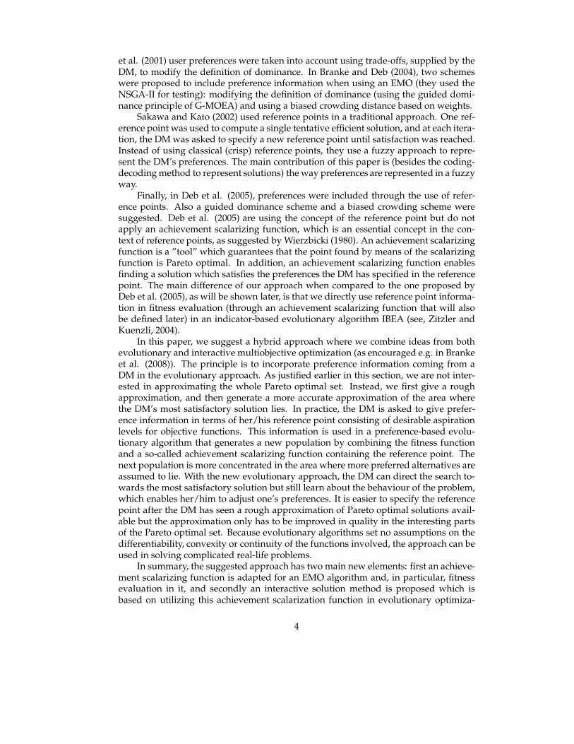
At first, we give simulation results using well-known two-dimensional benchmarkfunctions, namely ZDT1 and ZDT3, see Zitzler et al. (2000). As can be seen in Figure3, a run of the multiobjective optimizer IBEA for ZDT1 without preference informationyields a Pareto approximation containing points that are almost equally spaced (de-noted by triangles). When using the reference point (0.6, 1.0) (denoted by a big star)with a high specificity of δ = 0.1, a run of PBEA (denoted by stars) results in an ap-proximation that (a) dominates a part of the previous run without preferences and (b)is concentrated around the projected reference point (which has a circle around it). Re-member that by a projected reference point we mean a solution giving the minimumvalue for the achievement function used. In order to demonstrate the effect of decreas-ing specificity, we set δ = 0.02, and then, as discussed earlier, the concentration is evenmore visible (the points are denoted by boxes). Let us point out here that the optimalfront was not yet achieved because we used on purpose a small population size of 20in order to make the spacing of the solutions and development of different populationsmore visible. In the figure, one can see that when compared to the population obtainedusing IBEA (without preference information), using PBEA (with the same populationsizes and generation numbers) we get better solutions, that is, solutions that are closerto the actual Pareto optimal set. In other words, by including preference informationwe get a better approximation with the same computational effort, and from iterationto iteration the approximation gets more accurate, as will be seen in what follows.

Figure 4 represents a possible interaction with a DM using the preference basedalgorithm PBEA in ZDT1 with population size 20. At first, the DM performs a runwithout preference information with 300 generations and selects a point in the popu-lation as the reference point for the next iteration (with specificity δ = 0.05 and 400generations). This process is repeated again with a new reference point and a new runis performed with 500 generations. Now, a preferred solution from the last run is cho-sen as a reference point for a final run (with specificity δ = 0.02 and 500 generations) inorder to focus the search even more.

14

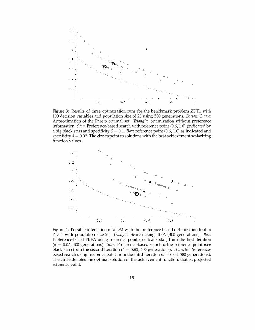
Figure 3: Results of three optimization runs for the benchmark problem ZDT1 with100 decision variables and population size of 20 using 500 generations. Bottom Curve:Approximation of the Pareto optimal set. Triangle: optimization without preferenceinformation. Star: Preference-based search with reference point (0.6, 1.0) (indicated bya big black star) and specificity δ = 0.1. Box: reference point (0.6, 1.0) as indicated andspecificity δ = 0.02. The circles point to solutions with the best achievement scalarizingfunction values.

Figure 4: Possible interaction of a DM with the preference-based optimization tool inZDT1 with population size 20. Triangle: Search using IBEA (300 generations). Box:Preference-based PBEA using reference point (see black star) from the first iteration(δ = 0.05, 400 generations). Star: Preference-based search using reference point (seeblack star) from the second iteration (δ = 0.05, 500 generations). Triangle: Preference-based search using reference point from the third iteration (δ = 0.03, 500 generations).The circle denotes the optimal solution of the achievement function, that is, projectedreference point.

15

Here, specificity (and the number of generations) was varied to demonstrate thatthis is possible but it is not necessary to vary the value between iterations. Let us againpoint out that we used small amount of generations and population sizes in order toclarify evolvement of the solution process. In practice, the approach can easily reach thePareto optimal set if the usual parameter settings for the population size and numberof generations are used.

The next three Figures 5, 6 and 7 show the effect of different locations of referencepoints, i.e., optimistic or pessimistic ones. To this end, we use another benchmark func-tion ZDT3, see Zitzler et al. (2000), which is characterized by a discontinuous Paretooptimal set. A run with IBEA without any preference information yields the set ofpoints shown in Figure 5 as triangles. It can be guessed that the Pareto optimal set con-sists of 5 disconnected subsets. A PBEA optimization using the pessimistic referencepoint (0.7, 2.5) (denoted by a black star) (with specificity δ = 0.03) yields the pointsshown as boxes. Again, they dominate points that have been determined using opti-mization without preference information and are concentrated around the projectionof the reference point (i.e., a solution with a circle). Similar results are obtained if anoptimistic reference point (0.4, 2.7) (with specificity δ = 0.02) is chosen, see Figure 6.The larger the distance between the reference point and the Pareto approximation, thesmaller is the effect of concentrating the search around the projection of the referencepoint. This can clearly be seen in Figure 7 where the optimistic reference point (0.3, 2.6)with (specificity δ = 0.01) is chosen. In all the figures, circles denote solutions with thebest achievement function value in the current population.

Figure 5: Results of two optimization runs for the benchmark problem ZDT3 with 100decision variables, population size 20 and 100 generations. Triangle: IBEA optimizationwithout preference information. Box: Preference-based PBEA with pessimistic refer-ence point (0.7, 2.5) (indicated by a big star) and specificity δ = 0.03. Circled solution isthe projected reference point.

Figure 8 is again based on runs for the benchmark problem ZDT3. Here, we usetwo reference points (0.25, 3.3) and (0.85, 1.8) (with δ = 0.03 each). This example modelsa DM who intends to concentrate her/his search on two areas of the Pareto approxima-

16

Figure 6: Results of two optimization runs for the benchmark problem ZDT3 with 100decision variables, population size 20 and 100 generations. Triangle: IBEA optimizationwithout preference information. Box: Preference-based PBEA with optimistic referencepoint (0.4, 2.7) (indicated by a big star) and specificity δ = 0.02. Circled solution is theprojected reference point.

Figure 7: Results of two optimization runs for the benchmark problem ZDT3 with 100decision variables, population size 20 and 100 generations. Triangle: IBEA optimizationwithout preference information. Box: Preference-based PBEA with optimistic referencepoint (0.3, 2.6) (indicated by a big star) and specificity δ = 0.01. Circled solution is theprojected reference point.

17

tion simultaneously. As can be seen, the search concentrates on the projections of thetwo reference points as expected.

Figure 8: Results of two optimization runs for the benchmark problem ZDT3 with 100decision variables, population size 20 and 100 generations. Triangle: IBEA optimiza-tion without preference information. Box: Preference-based PBEA with two referencepoints (0.25, 3.3) and (0.85, 1.8) (indicated by big stars) and specificity δ = 0.03. Circledsolutions are the projected reference points.

Finally, we consider one more problem with five criteria, see Miettinen et al. (2003).The problem is related to locating a pollution monitoring station in a two-dimensionaldecision space. The five criteria correspond to the expected information loss as esti-mated by five different experts. Therefore, the DM needs to find a location that balancesthe five possible losses. The problem formulation is as follows:

The decision variables have box constraints x1 ∈ [−4.9, 3.2], x2 ∈ [−3.5, 6]. Thecriteria are based on the function

f(x1, x2) = −u1(x1, x2)− u2(x1, x2)− u3(x1, x2) + 10

where

u1(x1, x2) = 3(1− x1)2e−x2

1−(x2+1)2

u2(x1, x2) = −10(x1/4− x31 − x5

2)e−x2

1−x2

2

u3(x1, x2) = 1/3 · e−(x1+1)2−x2

2 .

The actual objective functions to be minimized are

f1(x1, x2) = f(x1, x2)

f2(x1, x2) = f(x1 − 1.2, x2 − 1.5)

f3(x1, x2) = f(x1 + 0.3, x2 − 3.0)

f4(x1, x2) = f(x1 − 1.0, x2 + 0.5)

f5(x1, x2) = f(x1 − 0.5, x2 − 1.7).

18

In order to get a rough overview about the complexity of the problem, the follow-ing two Figures 9 and 10 represent a projected scan of the Pareto optimal set. They havebeen produced simply by probing the decision variables on a regular equidistant meshand selecting the Pareto optimal points from the set of solutions received. These twofigures demonstrate the need of preference based approaches and show how difficultit is to study approximations of Pareto optimal sets when the problem has more thantwo objectives.

Figure 9 shows solutions projected to the second and third dimension of the crite-rion space. The grey level of the points corresponds to the first criterion. In a similarway, Figure 10 shows the projection on the fourth and fifth criterion (and the grey levelagain indicates values of the first criterion). It can be observed that the optimizationproblem is highly non-linear and the Pareto optimal set is discontinuous.

Figure 9: Approximated Pareto optimal set of a multiobjective optimization problemwith 2 decision variables and 5 objective functions, see Miettinen et al. (2003). The pro-jection on objectives f2 and f3 is shown where the grey levels of the points correspondto values of f1.

Usually, in evolutionary approaches it is assumed that the graphical representa-tion of the Pareto front is self-explanatory and the DM can easily select her/his mostpreferred solution from there. Figures 9 and 10 demonstrate very clearly that this isnot necessarily the case with more criteria. It simply gets too difficult for the DM toanalyze the Pareto optimal solutions generated because (s)he can see only differentprojections of the 5-dimensional criterion space. When using the preference-based ap-proach, we do not need to illustrate the whole Pareto front but it is enough to provide arough approximation of it. The DM then directs the search by varying reference pointsand we can easily identify the best solution of the current population with the help ofthe achievement function. Thus, projections and other cognitively difficult visualiza-tions are not needed at all. In Table 1, we illustrate how our approach finds solutionscorresponding to different reference points, that is, their projections. (In all the runs,population size of 200 was used with 100 generations.)

In Table 1, the rows correspond to different runs of the evolutionary multiobjectiveoptimization algorithms, and the columns correspond to the two reference points that

19

Figure 10: For the same problem as in Figure 9, the projection on objectives f4 and f5 isshown where the grey levels of the points correspond to values of f1.

have been used to evaluate the achievement function. The objective vectors in the tablegive the best value for the achievement function in question (as mentioned in Step 3 ofthe interactive method). For comparative reasons, also the corresponding achievementfunction values are recorded even though they are not normally shown to the DM (asbefore, the smaller the value, the better the solution).

gref1 = (10, 10, 10, 10, 10) ref2 = (12, 11, 10, 9, 8)

IBEA f(x) (8.55, 7.54, 8,17, 9.61, 9.03) (9.72, 8.4, 9.94, 7.93, 6.83)sg(f(x)) -0.39 -0.06

PBEA f(x) (8.87, 8.99, 8,65, 8.84, 9.05) (9.21, 9.93, 9.29, 8.39, 7.64)δ = 0.1 sg(f(x)) -0.95 -0.36PBEA f(x) (8.95, 8.96, 8,60, 8.92, 8.96) (9.31, 10.0, 9.37, 8.39, 7.37)δ = 0.02 sg(f(x)) -1.04 -0.61

Table 1: Solutions giving minimal achievement function values for different referencepoints and values of achievement function (negative numbers).

The reference point ref1 = (10, 10, 10, 10, 10) represents preferred equal losses in thedifferent objectives of the problem. When the components of the weight vector w in (3)are equal, the algorithm is seeking for a solution where all values of objective functionsare as equal as possible. The other reference point ref2 = = (12, 11, 10, 9, 8) demonstrateshow preferring decreasing values is reflected in the solutions produced.

In Table 1, we can see that the preference-based evolutionary algorithm PBEAgives better solutions in terms of minimizing the achievement function than the ba-sic evolutionary approach IBEA. It means that the values of the objective functionsare more equal in the solution provided by PBEA than IBEA. In case of the first ref-erence point ref1 we find the achievement values -0.39 for IBEA and -1.04 for PBEA

20

(with specificity 0.02). In addition, a lower specificity leads to a better approximation(−1.04 < −0.95), as explained earlier. Similar observations hold for the second refer-ence point as well. The DM may continue by specifying a new reference point or byselecting the final solution as described in the interactive method in Section 4.

Out of curiosity, let us suppose, for example, that we look at the PBEA populationbased on reference point ref1 (and δ = 0.02) and try to find in this population a pointthat is closest to the other reference point ref2. Then the best point has an achievementfunction value of -0.05 which is much worse than the best value of -0.61 given in thetable. If we use the plain IBEA algorithm, i.e., no preference information is provided,then the point closest to the reference point ref2 has an achievement function value of-0.06 which again is much worse then -0.61. As a result we can say that it makes asubstantial difference whether we optimize with respect to a reference point used infitness evaluation, or some other reference point, as expected.

Our small illustrative example just demonstrates that the preference-based evolu-tionary approach is very helpful for the DM when (s)he wants to find the most pre-ferred solution for her/his multiobjective optimization problem involving more thantwo objectives. The DM does not have to study different projections (if (s)he does notwant to) because we can conveniently identify the best solution of the current popula-tion with the help of the achievement function.

Figure 11: Illustration of 70 solutions of the final population using value paths. Theexample screen is adopted from the implementation of the recent unpublished versionof VIMDA (Korhonen 1988).

If the DM, after all, wants to compare different solutions of the population, it ispossible to use, for example, value paths as mentioned in Section 4.2. In Figure 11, wehave 70 solutions of the last PBEA run with reference point ref1 and δ = 0.02. Eachcriterion is represented by a path and vertical lines correspond to solutions. The solu-tion denoted by a bold vertical line is the best solution listed in Table 1. As mentioned

21

earlier, this solution is balanced in terms of objective function values as the correspond-ing reference point is and this fact can be easily seen in the figure. In Figure 11, lowercriterion values are in the top part of the figure since they stand for more preferredvalues.

We have here demonstrated how PBEA can be used in the first iterations of ourinteractive algorithm. From here, the DM can continue by specifying a reference pointaccording to her/his preferences. Even from these examples one can see how concen-tration on a subspace of the Pareto optimal set means that the quality of the approxi-mation improves and the population sizes can be kept relatively small, which meanssavings in computational cost.

Let us point out that if computational cost is an important factor to consider, thereis no need to restart the optimization whenever a new reference point has been speci-fied. Instead, it is possible to include the nondominated solutions of the previous popu-lation into the temporary mating pool of the next iteration of the interactive algorithm.In this way, the diversity of an initial mating pool is combined with the knowledgeabout interesting regions of the search space. The search can now benefit from the pre-vious iteration if the new reference point is in the same subspace of the Pareto optimalset as the previous was. Otherwise, the old solutions will be removed in the environ-mental selection and new, better solutions will be generated in the region of interest.

6 Conclusions

We have introduced a new preference-based evolutionary algorithm that incorporatespreference information coming from a DM. By setting desirable values for objectivefunctions as a reference point, the DM can conveniently study such parts of the Paretooptimal set that (s)he finds interesting and the whole Pareto optimal set does not haveto be generated with equal accuracy and population sizes can be kept rather small.

In multiobjective optimization, reference points are projected to the Pareto opti-mal set with the help of achievement functions. Our innovative idea is to includean achievement function in the fitness evaluation of an evolutionary algorithm. Ourpreference-based evolutionary algorithm can be used as an integral part of an interac-tive multiobjective optimization algorithm. In this way, we get solutions in the neigh-borhood of the projected reference point (i.e., solutions concentrated around the refer-ence point projected to the Pareto optimal set) and we do not waste effort in comput-ing solutions in uninteresting areas. We can adjust how wide a neighborhood we areinterested in by setting a value for a specificity parameter. Adjusting the specificityparameter value is a topic for further research. (Naturally, using an interactive methodnecessitates that the DM has time and interest in taking part in the solution process.)

Our computational experiments indicate that the approximations produced uti-lizing reference point information give the DM reliable information on the solutionsavailable, the approximations get more accurate than without preference informationas well as from iteration to iteration and the DM can find the most preferred solution asthe final one conveniently. In addition, we have an intuitive way available for findinggood solutions in a population, that is, the achievement function used helps the DM inordering solutions and we are, thus, able to solve problems with more than two criteria.

In summary, our solution philosophy is different from the conventional EMO ap-proaches and it has the benefits of incorporating preference information (expressed inthe form easily understandable for the DM as a reference point), saving computationalcost and providing a convenient way of identifying the best solution of the currentpopulation (best reflecting the preferences expressed in the form of a reference point).

22

This last point is especially important as, when solving problems with more than twoobjectives, simple visualization is not enough to help the DM find the most preferredsolution. The idea of including preference information in fitness evaluation can be usedin other EMO approaches besides IBEA as well.

Acknowledgement

The research was partly supported by the Academy of Finland and the Jenny and AnttiWihuri Foundation. The authors wish to thank Prof. Roman Slowinski for his valuableideas.

References

Aittokoski T., Ayramo S., Miettinen K. (2008): Clustering aided approach for decision makingin computationally expensive multiobjective optimization. Optimization Methods and Software(to appear).

Benayoun R., de Montgolfier J., Tergny J., Laritchev O. (1971): Linear programming with multipleobjective functions: Step Method (STEM). Mathematical Programming, 1, 366–375.

Bleuler S., Laumanns M., Thiele L., Zitzler E. (2003): PISA - A Platform and Programming Lan-guage Independent Interface for Search Algorithms, in: C.M. Fonseca, P.J. Fleming, E. Zitzler, K.Deb, L. Thiele (Eds.), Evolutionary Multi-Criterion Optimization (EMO 2003), Springer-Verlag,Faro, Portugal, 494–508.

Branke J., Deb K. (2004): Integrating User Preferences into Evolutionary Multi-Objective Opti-mization, KanGal Report 2004, Indian Institute of Technology. Kanpur, India.

Branke J., Kaussler T., Schmeck H. (2001): Guidance in evolutionary multi-objective optimization.Advances in Engineering Software, 32, 499–507.

Branke J., Deb K., Miettinen K., Slowinski R. Eds. (2008): Multiobjective Optimization: Interac-tive and Evolutionary Approaches. Springer-Verlag, Berlin, Heidelberg.

Cvetkovic D., Parmee I. (1999): Genetic Algorithm-based Multi-objective Optimization and Con-ceptual Engineering Design, in: Proceedings of the Congress on Evolutionary Computation (CEC’99), vol. 1, IEEE Press, 29–36.

Cvetkovic D., Parmee I. (2002): Preferences and their application in evolutionary multiobjectiveoptimization. IEEE Transactions in Evolutionary Computation, 6(1), 42–57.

Chankong V., Haimes Y.Y. (1983): Multiobjective Decision Making Theory and Methodology,Elsevier Science Publishing, New York.

Coello C.A.C (2000): Handling Preferences in Evolutionary Multiobjective Optimization: A Sur-vey, in: Proceedings of the 2000 Congress on Evolutionary Computation, IEEE Service Center,Piscataway, NJ, 30–37.

Deb K. (1999a): Multi-Objective Evolutionary Algorithms: Introducing Bias Among Pareto-Optimal Solutions. KanGAL Report 99002, Indian Institute of Technology, Kanpur, India.

Deb K. (1999b): Solving goal programming problems using multi-objective genetic algorithms.In Proceedings of the Congress on Evolutionary Computation (CEC ’99), IEEE Press, 77–84.

Deb K., Sundar J., Uday B.R.N. (2005): Reference Point Based Multi-Objective Optimization Us-ing Evolutionary Algorithms. KanGAL Report 2005012, Indian Institute of Technology. Kanpur,India. And Proceedings of the 8th annual conference on Genetic and evolutionary computation,2006, Seattle, 635–642.

Fonseca C., Fleming P. (1993): Genetic Algorithms for Multiobjective Optimization: Formula-

23

tion, Discussion and Generalization, in: S. Forrest (Ed.), Proceedings of the Fifth InternationalConference on Genetic Algorithms, Morgan Kauffman Publishers, 416–423.

Geoffrion A.M., Dyer J.S., Feinberg A. (1972): An interactive approach for multi-criterion opti-mization, with an application to the operation of an academic department. Management Science,19, 357–368.

Greenwood G., Hu X., D’Ambrosio J. (1997): Fitness Functions for Multiple Objective Optimiza-tion Problems: Combining Preferences with Pareto Rankings, in: R. K. Belew, M. D. Vose (Eds).Foundations of Genetic Algorithms 4, Morgan Kauffman Publishers, 437–455.

Hanne, T. (2006): Interactive Decision Support Based on Multiobjective Evolutionary Algo-rithms, in: H.-D. Haasis, H. Kopfer, J. Schonberger (Eds.). Operations Research Proceedings2005, Springer-Verlag, 761–766.

Hwang C.-L., Masud A.S.M. (1979): Multiple Objective Decision Making - Methods and Appli-cations, Springer-Verlag, Berlin, Heidelberg.

Jaszkiewicz A., Slowinski R. (1999): The ’Light Beam Search’ approach - an overview of method-ology and applications, European Journal of Operational Research, 113, 300–314.

Klamroth K., Miettinen K. (2008): Integrating Approximation and Interactive Decision Makingin Multicriteria Optimization, Operations Research, 56, 222234.

Koopmans T.C. (1971): Analysis and Production as an Efficient Combination of Activities, in:T.C. Koopmans (Ed.), Activity Analysis of Production and Allocation (originally published in1951), Yale University Press, New Haven, London, 33–97.

Korhonen, P. (1988): A Visual Reference Direction Approach to Solving Discrete Multiple CriteriaProblems, European Journal of Operational Research, 34, 152–159.

Korhonen P., Laakso J. (1986): A visual interactive method for solving the multiple criteria prob-lem, European Journal of Operational Research, 24, 277–287.

Korhonen P., Wallenius J. (1988): A Pareto Race, Naval Research Logistics, 35, 615–623.

Kuhn H.W., Tucker A.W. (1951): Nonlinear Programming, in: J. Neyman (Ed.), Proceedings of theSecond Berkeley Symposium on Mathematical Statistics and Probability. University of CaliforniaPress, Berkeley, Los Angeles, 481–492.

Larichev O.I. (1992): Cognitive validity in design of decision-aiding techniques. Journal of Multi-Criteria Decision Analysis, 1, 127–138.

Luque M., Miettinen K., Eskelinen P., Ruiz F. (2009): Incorporating preference information ininteractive reference point methods for multiobjective optimization. Omega, 37, 450-462.

Massebeuf S., Fonteix C., Kiss L., Marc StateI., Pla F., Zaras K. (1999): Multicriteria Optimizationand Decision Engineering of an Extrusion Process Aided by a Diploid Genetic Algorithm, in:Proceedings of the Congress on Evolutionary Computation (CEC ’99), IEEE Press, 14–21.

Miettinen K. (1999): Nonlinear Multiobjective Optimization, Kluwer Academic Publishers,Boston.

Miettinen K. (2003): Graphical Illustration of Pareto Optimal Solutions, in: T. Tanino, T. Tanaka,M. Inuiguchi (Eds.), Multi- Objective Programming and Goal Programming: Theory and Appli-cations, Springer-Verlag, Berlin, Heidelberg, 197–202.

Miettinen K, Makela M.M. (1995): Interactive bundle-based method for nondifferentiable multi-objective optimization: NIMBUS. Optimization, 34(3), 231–246.

Miettinen K, Makela M.M. (2006): Synchronous approach in interactive multiobjective optimiza-tion. European Journal of Operational Research, 170, 909–922.

24

Miettinen K, Lotov A.V., Kamenev G.K., Berezkin V.E. (2003): Integration of two multiobjectiveoptimization methods for nonlinear problems. Optimization Methods and Software, 18(1), 63–80.

Miettinen, K., Molina, J., Gonzlez, M., Hernndez-Daz, A., Caballero, R.: Using box indices in sup-porting comparison in multiobjective optimization. European Journal of Operational Research.To appear (2008).

Nakayama H., Sawaragi Y. (1984): Satisficing trade-off method for multiobjective programming,in: M. Grauer, A.P. Wierzbicki (Eds.), Interactive Decision Analysis. Springer-Verlag, StateBerlin,113–122.

Olson D. (1996): Decision Aids for Selection Problems. Springer-Verlag, New York.

Pareto V. (1906): Manuale di Economia Politica. Piccola Biblioteca Scientifica, Milan, Note: Trans-lated into English by Ann S. Schwier (1971), Manual of Political Economy, MacMillan, London.

Parmee I., Cvetkovic D., Watson A., Bonham C. (2000): Multi-Objective satisfaction within aninteractive evolutionary design environment, Journal of Evolutionary Computation, 8 (2), 197–222.

Phelps S., Koksalan M. (2003): An interactive evolutionary metaheuristic for multiobjective com-binatorial optimization, Management Science, 49(12), 1726–1738.

Rekiek B., De Lit P., Pellichero F., LEglise T., Falkenauer E. and Delchambre A. (2000): Dealingwith User’s Preferences in Hybrid Assembly Lines Design. In Proceedings of the MCPL2000Conference.

Sakawa M., Kato K., (2002) An interactive fuzzy satisficing method for general multiobjective0-1 programming problems through genetic algorithms with double strings based on a referencesolution, Fuzzy Sets and Systems, 125(3), 289–300.

Sawaragi Y., Nakayama H., Tanino T. (1985): Theory of Multiobjective Optimization, AcademicPress, Orlando, Florida.

Steuer R.E. (1986): Multiple Criteria Optimization: Theory, Computation, and Application, JohnWiley & Sons.

Trinkaus H.L., Hanne T. (2005): knowCube: A visual and interactive support for multicriteriadecision making, Computers & Operations Research 32, 1289–1309.

Wierzbicki A. (1980): The Use of Reference Objectives in Multiobjective Optimization, in: G.Fandel, T. Gal (Eds.), Multiple Objective Decision Making, Theory and Application, Springer-Verlag, 468–486.

Wierzbicki A. (1986): On the completeness and constructiveness of parametric characterizationsto vector optimization problems, OR Spectrum, 8, 73–87.

Zionts S., Wallenius J. (1976): An interactive programming method for solving the multiple cri-teria problem, Management Science, 22(6), 652–663.

Zitzler E., Deb K., Thiele L. (2000): Comparison of multiobjective evolutionary algorithms: em-pirical results, Evolutionary Computation, 8(2), 173–195.

Zitzler E., Kuenzli S. (2004): Indicator-based Selection in Multiobjective Search, in: X. Yao, E.Burke, J.A. Lozano, J. Smith, J.J. Merelo-Guervos, J.A. Bullinaria, J. Rowe, P. Tino, A. Kaban, H.-P.Schwefel (Eds.), Parallel Problem Solving from Nature - PPSN VIII, 8th International Conference,Proceedings, Springer-Verlag, Berlin, 832–842.

25