a precision dc-potentiometer microwave - nasa · a precision dc-potentiometer microwave - ......

NATIONAL AERONAUTICS AND SPACE ADMINISTRATION

It".

Technical Report No. 32-887

A Precision DC-Potentiometer Microwave

-

Insertion - Loss Test Set J L

C. T. Ste/zr/ed

M. S. Reid

S. M. Petty

JET PROPULSION LABORATORY

CALIFORNIA INSTITUTE OF TECHNOLOGY

PASADENA, CALIFORNIA

March 15 1966

flrr- •-' ''rr r'-

NY

https://ntrs.nasa.gov/search.jsp?R=19660013519 2018-06-16T04:56:18+00:00Z

NATIONAL AERONAUTICS AND SPACE ADMINISTRATION

Technical Report No. 32-887

A Precision DC - Potentiometer Microwave Insertion-Loss Test Set

C. T. Ste/zr/ed M. S. Reid S. M. Petty

. D. P. D. Potter, Manager

Communications Elements Research Section

JET PROPULSION LABORATORY CALIFORNIA INSTITUTE OF TECHNOLOGY

PASADENA, CALIFORNIA

March 15, 1966

I PL TECHNICAL REPORT NO. 32-887

NOTE

M. S. Reid is at Jet Propulsion Laboratory on leave of absence from the National Institute for Telecommunications Research, Johannesburg, South Africa.

JPL TECHNICAL REPORT NO. 32-887

CONTENTS

I. Introduction ...................... 1

II. Equipment Description ................ 2

A. Initial Setup .................... 3 B. Measurement Procedure ................ 3 C. Performance ... . . . . . . . . . . . . . . . . . . 5

Ill. Precision Measurement Techniques ........... 6

A. First-Order Analysis ................. 6 B. Second-Order Analysis ................ 8

IV. Experimental Results ................. 9

V. Conclusion ..................... 14

Nomenclature ...................... 15

References ....................... 15

Appendix ........................

TABLES

1. Difference between measured and calibrated insertion loss for H-band rotary-vane attenuator ............. 5

2. Insertion-loss measurements of WR 430 Waveguide Part No. 239, Set No. 2 (first-order analysis) at 2295 Mc ...........11

3. Insertion-loss measurements of WR 430 Waveguide Part No. 239, Set No. 2 (second-order analysis) at 2295 Mc ..........11

4. Mean insertion loss of WR 430 Waveguide Part No. 239 at 2295 Mc ......................11

5. Summary of 2295-Mc insertion-loss measurements of WR 430 Waveguide components ................. 12

6. Estimated accuracy of microwave insertion-loss test set ..... . 14

Iv


FIGURES

1. Block diagram of microwave insertion-loss test set ........ 2

2. Photograph of insertion-loss test set with an 8448-Mc waveguide configuration ..................... 3

3. Detail schematic of the test-set configuration .......... 4

4. Stability recording of microwave insertion-loss instrumentation . . . . 5

5. Measured attenuation diffeience versus attenuation for three thermistor mounts ................... 6

6. First-order insertion-loss data reduction ............ 7

7. Photograph of the WR 430 Waveguide microwave calibration heads of insertion-loss test set ............... 9

8. Photograph of WR 430 Waveguide liquid-nitrogen-cooled termination assembly .................. 10

9. Experimental insertion-loss data for Part No. 239, Set No. 2, with best least-squares straight line ............. 12

10. Experimental insertion-loss data for Part No. 239, Set No. 2, with best second-order least-squares curve ........... 12

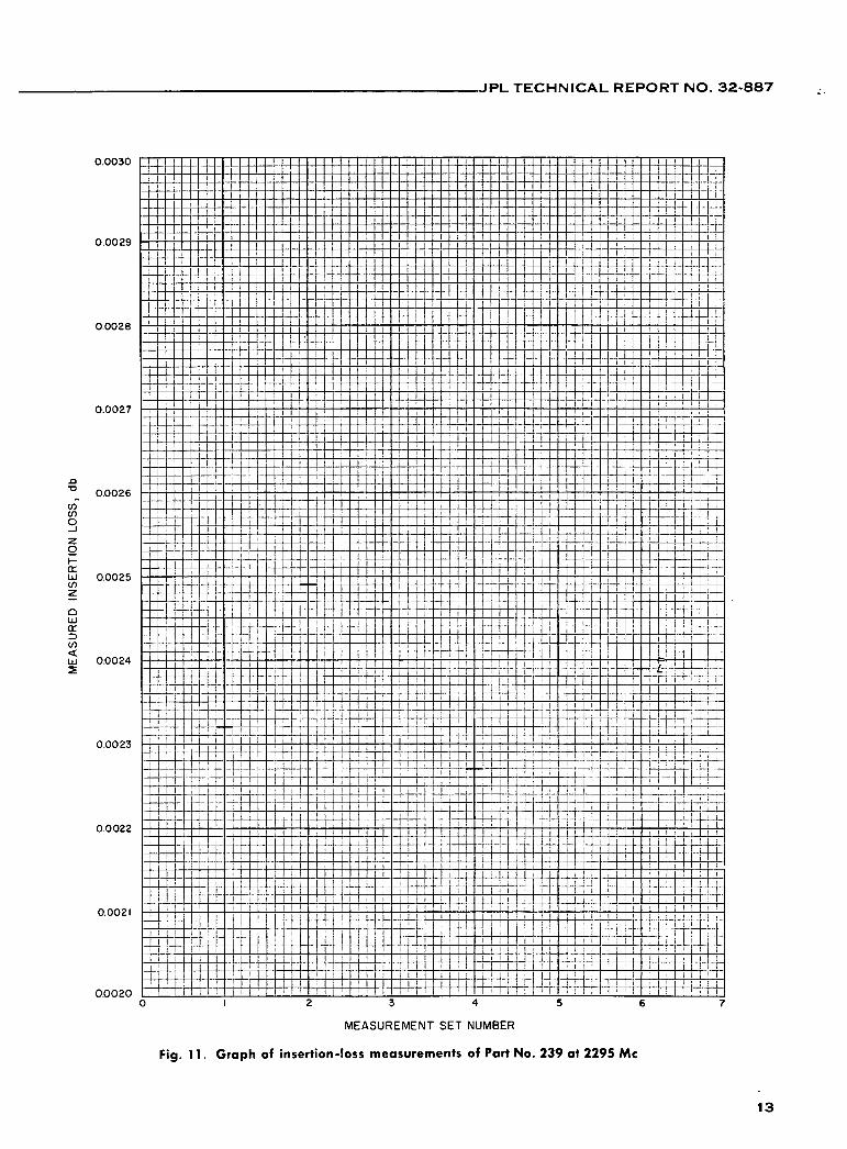
11. Graph of insertion-loss measurements of Part No. 239 at 2295 Mc ....................... 13

V


ABSTRACT

A requirement has existed at the Jet Propulsion Laboratory (JPL) for an instrument capable of measuring the insertion loss of transmission-line components beyond the normal precision capability of commer-cially available equipment. These measurements are necessary for the calibration of low-noise microwave receiving systems used in planetary/lunar astronomy and space communications programs. The instrumentation which was developed has a short-term jitter of 0.0004 db peak-to-peak and long-term drift of typically 0.0015 db/hr. Accuracy of the measurements is limited at the higher insertion-loss values by a 0.1% instrumentation nonlinearity. The precision at very low insertion-loss levels is shown to be better than 10 db. Details of the precision measurement techniques are presented for WR 430 Waveguide components.

I. INTRODUCTION

Accurate measurements of the parameters of passive microwave components are required in the assembly and evaluation of low-noise microwave receiving systems (Ref. 1). These measurements are used in the calibrations that are needed in the planetary and lunar radar ex-periments, radio astronomy, and space communications systems that form part of the program of Supporting Research and Advanced Development for the Deep Space Instrumentation Facility (DSIF) of JPL.

Thus there arose a need for an instrument that could measure the insertion loss of low-loss coaxial and wave-guide components in the Laboratory as well as at the Goldstone Tracking Station, and which could do this beyond the normal precision capability of commercially available equipment. At that time the most precise, com-mercially available test set was the Weinschel Dual Channel Insertion Loss Test Set .(Ref. 2), which has a precision of 0.02 db per 10 db (or 0.01 db, whichever is


greater). This test set is essentially a laboratory system and its precision did not meet the JPL requirements. Measure-ments of the required precision had, however, been achieved (Ref. 3) but at the cost of extreme care and extraordinary temperature stabilization. Two suitable systems were developed at JPL. One uses an ac ratio-transformer technique (Ref. 4) and, in common with

commercial insertion-loss test sets, requires modulation of the signal source. This Report describes the other system, which is a dc-potentiometer method. The dc-potentiometer test set does not require modulation of the signal source, eliminates ac ground-loop problems, incorporates increased temperature stability, can be operated from ac mains or batteries, and is portable.

II. EQUIPMENT DESCRIPTION

A dual-channel insertion-loss test set (Fig. 1) has been constructed almost entirely from commercially available equipment and components. The signal level is sampled with power meters at two points, and the dc outputs are compared on a null indicator. Amplitude instabilities in the signal generator do not affect the null, except for nonlinearity effects in the power meters. A precision divider is used to obtain a null both before and after inserting the microwave component to be measured at Point A. The difference in the divider ratio (converted to db) is a measure of the insertion loss of the component.

SIGNAL GENERATOR

COAXIAL OR WAVEGUIDE

UNKNOWN INSERTION POINT A

I IDIRECTIONALI I I 'MATCHING ISOLATORS COUPLER , I I 10 db I1 SECTION FH MATCHING1 COUPLER, MATCHED

SECTION I I 10 db I I LOAD

POWER POWER METER I METER

BRIDGE CIRCUIT

tRI IOOOS1 I R2I000XL

OHN FLUKE MODEL 605 NULL S-PLACE READOUT I VOLTMETER POTENTIOMETER

Fig. 1. Block diagram of microwave insertion-loss test set

The technology of precision dc dividers is more than ade-quate for the accuracy required. A photograph of the test set is shown in Fig. 2 in a configuration utilizing WR 112 Waveguide components. The waveguide is matched with screw tuners so that the voltage standing wave ratio (VSWR) in either direction from Point A is less than 1.01.

The internal circuitry of the power meter has an out-put which is proportional to the square root of the applied power. In order to have a linear output with respect to power, a squaring circuit used on the output of the power meters gives straight-line segments approximating square-law nonlinearity. The output linearity of the power meters was greatly improved by utilizing the output across the feedback resistor,' thereby bypassing the squaring-circuit output. A detail schematic of the test set is shown in Fig. 3.

Switch S1A, in the power meter circuitry, enables the power meters to be operated in the normal manner when not used to measure insertion loss. Switch S, is a two-pole, four-position switch in the comparator circuitry. Positions 1 and 2 are used with the zero adjustment for Power Meters 2 and 1, respectively, to set the bias with RF power removed. This bias sets the quiescent current of the transistors in the feedback paths to the power meters. Position 4 is used to balance the - 18-v power-meter sup-plies with R,, and to define the null position between the power meters when the - 18-v supplies are slightly out of balance, just prior to the final readout-potentiometer null adjustment. A steady-state unbalance between the - 18-v

'Suggested by Mr. F. Praman of Hewlett—Packard, Palo Alto, Calif. These are Resistors R160—R166 shown in Fig. 5-3 of HP Instntction Manual for the HP 431B power meter.

2


5

Fig. 2. Photograph of insertion-loss test set with an 8448-Mc waveguide configuration

supplies is a source of measurement nonlinearity. In-correct changes in the - 18-v balance between readings reduces the insertion-loss measurement resolution. Posi-tion 3 is the final readout position. The 5000-ohm helipots in the bridge circuit can be set so that a full-scale read-ing on the power meter is obtained with RF power applied (after Step 1 in the measurement procedure). This is done only as an initial setting, and is convenient for occasionally checking the HF power level.

A later version of the test set which uses a common power supply eliminated the need for the equalizing adjustment of the power supplies.

Modulation of the signal source is not required with the Hewlett—Packard HP 431B Power Meter, thus eliminating possible errors from klystron signal-source double moding and modulator instability. A stability test was made of the test set by recording the output of the null voltmeter; a typical data sample is shown in Fig. 4. Short-term jitter is about 0.0004 db peak-to-peak, and long-term drift is typically 0.0015 db/hr.

The operating instructions for the test set are as follows:

A. Initial Setup

1. With Switch S . in the normal power-meter position (Transistor Q107 connected to the power-meter

range switch), perform the normal power-meter zero-ing and nulling.

2. Set the signal-generator power level (typically 1.5 mw).

B. Measurement Procedure

1. Switch SA to the external range resistor.

2. Remove the HF power.

a. Switch S, Position 4: adjust R for a zero (±0.5 my) on the null voltmeter.

b. Switch S, Position 1: adjust zero for Power Meter 2 for 45 my (±2 my) on the null voltmeter.

c. Switch S, Position 2: adjust zero for Power Meter 1 for a null (±2 my) on the null voltmeter.

3. Apply HF power and Switch S to Position 3.

4. Adjust the precision potentiometer for a null and record the reading ratio.

These steps are repeated several times with the wave-guide parts connected together first without the unknown and then with the unknown inserted at Point A in Fig. 2. The ratios are converted with tables to db and then differences are taken and averaged.

3

JPL TECHNICAL REPORT NO. 32.887

SIGNAL I GENERATOR UNKNOWN INSERTION

POINT A

ISOLATORSDIRECTIONAL H MATCHING MATCHING

COUPLERk^ SECTION SECTION 10 d

DIRECTIONAL COUPLER

TERMINATION 10 d

POWER

POWER 0107 METER I

METER 2

-18 v

REGULATED

RANGE SWITCH SIO2

-18 v

REGULATED

RI NTED

ec

PRIED -- j°51 11: CIRCUIT CIRCUIT

J GROUND GROUND RANGE

SWITCH SIO2

4.7 k

100 n IOO

50OO-

HELIPOT

HELIPOT

H L IOOO

40 0^ 1%

I 2 3 4 4 3 2 I S1

POTENTIOMETER 4-POSITION 2-POLE SWITCH FLUKE MODEL 60A I. POWER METER 2 BIAS

ADJUSTMENT 2. POWER METER I ZERO

ADJUSTMENT 3. OPERATION

--t4. -18-v ADJUSTMENT

I -COMPARATOR CHASSIS

*COMPONENTS ADDED TO POWER METER CIRCUITRY . NULL

VOLTMETER

Fig. 3. Detail schematic of the test-set configuration

4


5 mm

0.00 I—db CALIBRATION

Fig. 4. Stability recording of microwave insertion-loss instrumentation

C. Performance

As an example of typical test-set performance, a right-angle WR 112 Waveguide section was measured eight consecutive times.

1. Average insertion loss was 0.0282 db.

2. Maximum difference from this average was 0.0017 db.

3. Average difference of all measurements from 0.0282 db was 0.0008 db, which includes the nonrepeata-. bility of connecting and disconnecting waveguide flanges.

Many insertion-loss measurements of other components have been made with comparable results (Ref. 5).

The measurement of linearity of an insertion-loss test set is very difficult. One method used with limited success was to measure attenuators separately and in various combinations. The measured insertion loss of the com-binations should be that obtained by summing the indi-vidually measured insertion losses. This method is time consuming and is especially vulnerable to mismatch errors. The most successful technique used a WR 112 Waveguide Hewlett—Packard Model H-382A Rotary Vane Attenuator, Serial No. 1103, which was modified, for high angular resolution and calibrated (Test No. 805434) by the National Bureau of Standards (NBS). The calibration frequency was 8448 Mc. Table 1 shows the difference between the NBS calibrations and the insertion-loss test set for three separate Hewlett—Packard Model 478A Thermistor Mounts over an attenuation range from 1.0 to 20 db. The indicated nominal attenuation is the amount of attenuation change produced by rotating the vane through the required angle. The variable at-tenuator is not removed from the microwave test set during these measurements. The RF power applied to the thermistors was 1.5 mw and the dc bias was 45 my for these tests. Figure 5 shows a plot of the attenuation differences. It was observed that a change of 5 my in the bias resulted in approximately 0.02 db change in the readout of 20 db. It is more important that the bias not change with high attenuations than with low attenuations. The NBS "estimated accuracy" is shown in dotted lines. The difference in db as compared with the precision H-band rotary-vane attenuator is less than 0.10% for nominal values of attenuation in db to 16 db for these three particular thermistor mounts.

'Measurement Specialties Laboratory, Inc., Model H 200, Ser. 101.

Table 1. Difference between measured and calibrated insertion loss for H-band rotary-vane attenuator

Calibrated attenuator

Calibration (National Bureau of Standards), db, minus measured insertion loss

Thermistor Thermistor Therimstor setting, db mount Serial mount Serial mount Serial

8506 7731 8525

1.0 —0.0003 +0.0010 +0.0013

3.0 +0.00032 +0.0033 +0.0051

6.0 +0.0055 +0.0040 +0.006

10.0 +0.002 +0.004 +0.007

16.0 —0.019 —0.008 +0.002

20.0 —0.045 —0.031 —0.017

5

NATIONAL BUREAU OF STANDARDS

— -

I ESTIMATED ACCURACY TEST 805434 ThN/

--.-----

\\

____

HEWLETT — PACKARD THERMISTOR MOUNTS \

o SERIAL 8506\

\ SERIAL 7731

o SERIAL 8525

LL!J

0.12

0.OE

-D

li-i 0.04 0 Z w cr w LL Li

C z 0

I-

2

Lu —0.04 I—I—

-0.08

—0.120


ATTENUATION, db

Fig. 5. Measured attenuation difference versus attenuation for three thermistor mounts

III. PRECISION MEASUREMENT TECHNIQUES

A. First-Order Analysis

For precision measurements (accuracy on the order of 10-), statistical methods are required. The least-squares method (Ref. 6) can be used to advantage. A plot of the measured insertion-loss data y can be made as a function of measurement number m. For relation to drift error, this method must assume a uniform time spacing of measurements. Experimentally, this can be realized to a good approximation. A best-fit straight line can be determined from the modified data points (Fig. 6). The modified data points are obtained from the original data

points y by adding a constant L/2 to each power-level measurement with the unknown disconnected, and sub-tracting L/2 from each power-level measurement with the unknown connected. The standard deviation if of the modified data points from the best-fit straight line a + bx is

()2 = (y + L/2 - a - bx)2

+--- (y_L/2_abx)2 (1)

6


Rearranging, Y2

Y4•

tY3 Ym

V

- L-- +am+bx=y

(3)

Solving for L,

® ORIGINAL DATA POINTS . MODIFIED DATA POINTS

2 3 4 5

MEASUREMENT NUMBER, x

Fig. 6. First-order insertion-loss data reduction

where

y = Insertion-loss test-set reading, db

x = Measurement number

L = Average measured insertion loss, db

a = Constant of best-fit straight line, db

b = Slope of best-fit straight line, db/measurement number

m = Total number of measurements

o Odd measurements (unknown disconnected)

e = Even measurements (unknown connected)

In order to determine the values of a, b, and L fot which the standard deviation is a minimum, Eq. (1) is differentiated with respect to a, b, and L, and is equated to zero (Ref. 6, p. 240).

(y+L/2—a—bx) +.(y — L/2—a— bx) =0

x(y + L/2 - a - bx) + x(y - L/2 - a - bx) = 0

(y+L/2—a—bx) —(y—L/2--a— bx) =0

(2)

M

XY X

- (y — y) 1 (x — x)

L=2—1 rn

—(x —x) Ex EX2

—m 1 (x —x)

(4)

A simplification can be made if the middle measure-ment number is chosen as the origin so that the sum-mation of all odd powers of x is zero (Ref. 6, p. 252). This is discussed in more detail in Section IV. Then,

-

L= (m— 1)/2 (m±1)/2

ae+

rn — i m+1

b X2

The probable errors of the odd and even data points are (Ref. 6, p. 167)

/ [y + (L/2) —a—bx]2\½ PE,,, = 0.6745( (in + 1)/2

(6) / [y - (L/2) - a - br]2

PE, = 0.6745(m - 1)/2

)½

By expanding L in terms of the coefficients of the data points and summing (Ref. 6, p.229), the probable error FEZ of the mean insertion loss L is found to be

E-+

- /_(PE 0) 2

(PE,, )2\½ -

(m - 1)/2 (m -1)/2)

rA


B. Second-Order Analysis

In many applications of insertion-loss measurement, the maximum precision is required. For example, the accurate calibration of cooled microwave terminations is of funda-mental importance to the evaluation of low-noise receiving systems. The precision measurement of the insertion loss of the transmission-line components is a basic require-ment in the calibration of the termination. In view of the wide application and great importance of high-precision insertion-loss measurements, a second-order statistical analysis of the data reduction method has been carried out. The derivation is similar to the first-order analysis and is detailed in Appendix A.

The second-order analysis fits a parabola a' + b'x + c'x2 to the modified data points (Fig. 6). This accounts for both drifts that occur at a constant rate and drift rates that change at a constant rate during the measurement period. The constant b' is the drift rate, or drift per measurement number in db, and is equal to b in the first-order analysis. The constant c' is the rate of change of the drift rate. The analysis minimizes the standard deviation a' of the modified data points from the best fit parabola and yields

and the probable error of the mean insertion loss is

PE = ([PEyo] 2 a2 + [PEye] 2 a2 1Y/2 (13)

where a, the coefficients of the data points, are given by

a =-;{ [X2 + (m - 1)x - (X2)212(m1)

- 2[x2 + (m - 1)x _(x2)2} [mX - X2]

X x2+[mX-x2]2x4} (14)

and

a2{[x2_(m+1)x4+(x2)2]2(m21)

-2 [ :X 2 X2 - (m+ X4 + (2 X2)2]

X (15)

L - x2y[mX X2] +Y[mx - ( X2)2]) (8)

_1 [_x4+kx2]} (9)

Y= Exy (10)

+X[_x2 +m]} (11)

where

=(-1)[Kx2 +X[mX — 2 X21 - m[mx X2)2]

= x2 - x2 0

The probable errors of the data points are

[y + (L/2) - a' - b'x - C'X2]2 PE 0 = 0.6745

/ °

(m + 1)/2

)½)

[y - (L/2) - a' - b'x - C'X2} PEye = 0.6745

(m - 1)/2

2 )½ f (12)

Equations (5)—(13) have been programmed for an IBM 1620 Computer (Appendix B), and are used with the insertion-loss measurement data reduction. If the probable errors resulting from the use of Eqs .. (6) or (12) indicate significant difference between odd and even point values, a fault is indicated in one of the transmission-line connections. The probable errors given by (6) and (7)—and (12) and (13)—are due only to the random

8

PL TECHNICAL REPORT NO. 32-887

measurement errors and do not indicate bias or non-linearity errors.

Measurement data for a precision insertion-loss evalu-ation may be reduced both by the first-order and the

second-order analyses. This technique yields two values for the mean insertion loss, each with an associated probable error. The value of L from the data reduction technique which gives the smaller probable error is chosen.

IV. EXPERIMENTAL RESULTS

This section describes part of one application of the dc-potentiometer test set to the high-precision measure-ment of microwave insertion loss. This task was the calibration of a liquid-nitrogen-cooled waveguide termi-nation at 2295 Mc. The calibration required the precision measurement of the insertion loss of various WR 430

Waveguide transmission-line sections as well as the evaluation of a silicone grease film and a mylar window between waveguide flanges.

The WR 430 Waveguide microwave calibration heads for the insertion-loss test set are shown in Fig. 7. The

Fig. 7. Photograph of the WR 430 Waveguide microwave calibration heads of insertion-loss test set

9

p.

6

PART NO 239\


special heavy flanges are pinned for proper waveguide alignment. The VSWR was evaluated with a precision waveguide sliding termination and reduced to less than 1.005. Each transmission-line test section (Part Nos. 226 and 239) shown in Fig. 8 was measured, as well as a sec-tion of copper waveguide (Part No. 240) and various combinations of No. 239 and No. 240. The insertion loss of Nos. 226 and 239 is fundamental to the calibration of the cooled termination. Part No. 240 was examined in order that the silicone grease film and the mylar window could be evaluated in conjunction with No. 239.

Part No. 226 is a stainless steel WR 430 \Vaveguide sec-tion 4.0 in. long. It has a wall thickness of 0.025 in., and

copper plating and gold flash on the inside of 0.000120 in. and 0.000010 in. respectively. It is filled with a half-wavelength piece of polystyrene foam. The VSWR of this section is less than 1.005. The polystyrene window is required to prevent moisture condensation which will form on thin membrane windows. Part No. 239 is a 4.0-in, length of brass waveguide section with an indite plate. Part No. 240 is a 4.0-in, length of copper waveguide section.

The following insertion-loss measurements were made:

Part Nos. 226, 239, and 240 alone.

Part Nos. 239 and 240 in combination.

INCHES

Fig. 8. Photograph of WR 430 Waveguide liquid-nitrogen-cooled termination assembly

EI!


Part Nos. 239 and 240 with a 0.001-in.-thick mylar window between them.

Part Nos. 239 and 240 with a thin silicone grease film on their mating flanges.

Five sets of eleven measurements were made on each unknown. After every set the match of each calibration head was checked and corrected if the VSWR became 1.005 or worse. The flanges of the calibration heads and of the unknown were lapped after every set as well. All of the waveguide flanges were pinned except the stainless steel Part No. 226. This section was aligned with the bolt holes using a drill rod before bolting together.

Table 2. Insertion loss of WR 430 Waveguide Part

No. 239, Set No. 2 (first-order analysis) at 2295 Mc

Ratio R y, dbDifference from straight-line fit,

dbXlO3

Insertion loss L db

0.99665 0.029146 -0.34339 0.00244

0.99637 0.031586 -0.12339 0.00244

0.99665 0.029146 0.18900 0.00218

0.99640 0.031325 0.14748 0.00279

0.99672 0.028536 0.11137 0.00227

0.99646 0.030802 0.15686 0.00279

0.99678 0.028013 0.12091 0.00200

0.99655 0.030017 -0.09520 0.00244

0.99683 0.027577 0.21763 0.00192

0.99661 0.029494 -0.08575 0.00296

0.99695 0.026532 -0.29551

First-order constants: a = 0.02940 db

b = -0.00027 db/measurement

Mean insertion loss: I = 0.00249 db

Probable errors: PE,. = 0.00029 db

PE5, = 0.00008 db

PEZ = 0.00007 db

Table 2 shows a typical data set taken on Part No. 239. This table is also the format of the computer output for the straight-line (first-order) analysis. The first column lists the readings taken. The y values in the second column are those ratios converted to db by

- y=20log10 R (16)

The third column shows the difference of each y value from the straight-line fit and the last column is the in-sertion loss in db for each pair of readings. The probable errors from Eqs. (6) and (7) are also shown. The same data are shown in Table 3 with the second-order analysis and are plotted in Figs. 9 and 10. The translations in the

Table 3. Insertion loss of WR 430 Waveguide Part

No. 239, Set No. 2 (second-order analysis)

at 2295 Mc

Ratio R y, db

Difference from second-order

curve, db X iO

Insertion loss L, db

0.99665 0.029146 -0.09634 0.00244

0.99637 0.03 1586 0.02484 0.00244

0.99665 0.029146 0.13959 0.00218

0.99640 0.03 1325 0.07337 0.00279

0.99672 0.028536 -0.08627 000227

0.99646 0.030802 0.00864 0.00279

0.99678 0.028013 -0.07672 0.00200

0.99655 0.030017 -0.16931 0.00244

0.99683 0.027577 0.16822 0.00192

0.99661 0.029464 0.06249 0.00296

0.99695 0.026532 -0.04847

Second-order constants: a' = 0.02958 db

= 0.00027 db/measurement

= -0.00002 db/(measurement)'

Mean insertion loss: L = 0.00242 db

Probable errors: PE,, 0.00007 db

PE,,, 0.00006 db

PEI 0.00004 db

x-axes used for simplification of the analysis consist of subtracting the middle measurement number from each original measurement number. In order to expand the scale, the constants a and a' are subtracted from the first- and second-order curves respectively and also from the data points modified by L/2. The curves pass through the origin due to the scale translations. The ex-perimental points in Figs. 9 and 10 may not have the same appearance because different L/2 values are added to and subtracted from the odd and even data points.

The averages for the five sets of independent measure-ments for Part No. 239 are shown in Table 4 using the

Table 4. Mean insertion loss of WR 430 Waveguide

Part No. 239 at 2295 Mc

Measurement set No.

Mean insertion less L, db

Probable errors

PE50, PE,,, PEL, db db db

1 0.00232 0.00024 0.00018 0.00013

2 0.00249 0.00010 0.00007 0.00006

3 0.00222 0.00014 0.00012 0.00009

4 0.00229 0.00015 0.00006 0.00007

5 0.00242 0.00007 1 0.00006 1 0.00004

11


jul11

• .

C

I I I I -5 -4 -3 -2 -1 0\ I 2 3 4 5 MEASUREMENT NUMBER, x S

.

-0.00

I I I I I

Fig. 10. Experimental insertion-loss data for Part No. 239, Set No. 2, with best second-order

least-squares curve

Table 5. Summary of 2295-Mc insertion-loss measurements of WR 430 Waveguide

components

0.002

p..- S

S

C

I I I I '".'i.,. I I I I -5 -4 -3 -2 -I 0\ I 2 3 4 5 MEASUREMENT NUMBER, x

S

s'.I.i

S

S

-0.002

I I I I I I

Fig. 9. Experimental insertion-loss data for Part No. 239, Set No. 2, with best least-squares straight line

curve with the lowest probable error for L. The mean insertion loss for each set L1 to L5 is shown as well as probable errors of the odd and even y values, and, finally, the probable error of the mean insertion loss of each set. The weighted mean of the insertion loss is then found with the probable error of each set used as a weighting factor, and the grand mean L is shown in Table 5. The average measured insertion loss of each set is shown as a horizontal bar in Fig. 11. The associated probable errors are shown as vertical lines. The grand weighted mean L and its probable error are also shown.

Part No. Description Insertion loss db

Probable error of i db X 10'

226 Stainless steel 0.00690 0.33

239 Brass 0.00239 0.28

240 Copper 0.00118 0.31

2391 240 Sum 0.00357 0.42

2391 240 Combination 0.00358 0.38

2391 With mylar 2401 window

0.00413 0.27

2391 With silicone 2401

0.00355 0.29 grease

12

0.0030

0.0029

0.0028

0.0027

D 0.0026 U) U)

z 0 I—

w 0.0025 (n z

0 w cr

(I) 4 ILl 0.0024

0.0023

0.0022

0.0021

0.0020

___JPL TECHNICAL REPORT NO. 32-887

MEASUREMENT SET NUMBER

Fig. 11. Graph of insertion-loss measurements of Part No. 239 at 2295 Mc

13


A nonweighted mean L' of L 1—L5 was also calculated with its associated probable error. This mean differed at most by a few parts in 10 from the weighted mean. If the probable error of E' were appreciably greater than the probable error of L, bias errors would be indicated for some of the individual sets. Measurement time is approximately 3 hr for the five sets of readings required for a grand mean.

The insertion loss of the brass waveguide Part No. 239 is shown to be 0.00239 db with a probable error of 0.28 X 10 db; the insertion loss of the copper Part No. 240 is 0.00118 db with a probable error of 0.31 X 10 db. The sum of these two insertion losses is 0.00357 db, with their probable errors combined as 0.42>< 10 db. This sum, 0.00357 db, must be compared with the measured value of the insertion loss of Nos. 239 and 240 in combi-nation, which is 0.00358 db—a difference of 10 db. The probable errors of the sums are slightly higher than the probable errors of the combinations, as expected.

The theoretical insertion loss for No. 240 (copper wave-guide 4 in. in length) is 0.00091 db (Ref. 7). This theo-retical value does not account for surface roughness, metal impurities, or nonhomogeneity. A correction estimate for

surface roughness increases the insertion loss by 15% (Ref. 7) to 0.00105 db. This agrees with our measurement to within 0.00013 db.

Part No. 240 was then used in conjunction with No. 239 to evaluate a 0.001-in.-thick mylar window. This material is presently under consideration as an additional window. Table 5 shows that the excess insertion loss due to the mylar window is 0.0055 db with a probable error of less than 10 db.

A thin silicone grease film is sometimes required be-tween the flanges of waveguide sections of dissimilar metal. This film helps prevent corrosion which changes the insertion loss. The effect of a silicone grease film between the flanges of Nos. 239 and 240 was investigated. The results are presented in Table 5 and these show that (a) the effect of the film on the insertion loss is negligible, and (b) the insertion loss appears to drop when the grease is added. The lower insertion loss in (b) may be apparent, and explained by the spread of the probable errors. On the other hand, this effect may be real and the insertion loss lower owing to the high dielectric constant of the grease filling the low spots of the flange face and thus decreasing the reactance.

V. CONCLUSION

The average of the probable errors of the measured values of L from Table 5 is 0.31 X 104 db. It may be concluded, therefore, that if statistical methods are used with a sufficient number of observations, and if the measurement procedure is carried out as described with the indicated precautions, then insertion loss can be measured with a probable error of less than 10- 4 db. This does not include the bias and nonrandom errors and waveguide tolerance errors. The estimated overall ac-curacy of the test set, expressed in terms of the insertion loss measured, is tabulated in Table 6.

The upper operating frequency is presently limited to 40 Gc by the thermistor mount characteristics of the

Hewlett—Packard 431B Power Meter, although the test set has operated at frequencies as high as 90 Gc with transitions, resulting in slight performance degradation.

Table 6. Estimated accuracy of microwave insertion-loss test set

Insertion-loss measurement Accuracy, db

range, db

0-10 ±0.0001 ±0.1% of measurement value in db

10-15 ±0.5% of measurement value in db

15-20 ± 1.0% of measurement value in db

14

___JPL TECHNICAL REPORT NO. 32-887

NOMENCLATURE

a

at

b

In

C,

e Even measurements (unknown connected)

L Mean insertion loss from one set of measure-ments

E Mean of mean insertion losses from several sets of measurements

m Total number of data points in single measure-ment set

o Odd measurements (unknown disconnected)

PE,, Probable error of a

FE,, Probable error of b

Probable error of c

Probable error of L

Probable error of even data points

Probable error of odd data points.

SiSwitches

SIA

x Measurement number

X X2 X2

y Data point

a Coefficients of data points

Determinant on x and m

a Standard deviation

PE

PE

First- and second-order analysis coeilcients FE11,

- FE9,,

REFERENCES

1. Stelzried, C. 1., "Temperature Calibration of Microwave Thermal Noise Sources," IEEE Transactions on Microwave Theory and Techniques, Vol. MTT-13, No. 1,

Correspondence, January 1965, P. 128.

2. Weinschel Engineering, Gaithersburg, Maryland, Application Note No. 4, 1962.

3. Engen, C. F., and Beatty, R. W., "Microwave Attenuation Measurements with Ac-curacy from 0.0001 to 0.06 db over a Range of 0.01 to 50 db," Journal of

Research of the National Bureau of Standards, Section C. Engineering and In-

strumentation, Vol. 64 C, April—June 1960.

4. Finnie, C. J., Schuster, D., Otoshi, T. Y., AC Ratio Transformer Technique for Pre-

cision Insertion Loss Measurements, Technical Report No. 32-690, Jet Propulsion Laboratory, Pasadena, California, November 1964.

5. Stelzried, C. T., and Petty, S., "Microwave Insertion Loss Test Set," IEEE Transactions

on Microwave Theory and Techniques, Vol. MU-i 2, No. 4, July 1964, p. 475.

6. Worthing, A. G., and Geffner, J., Treatment of Experimental Data, New York:

John Wiley and Sons, 1960.

7. Harvey, A. F., Microwave Engineering, New York: Academic Press, 1963, p. 46.

15


APPENDIX A

Derivation of the Second-Order Equations

The measured data points are modified in the same manner as in the first-order analysis. A constant L/2 is added to each power-level measurement with the unknown disconnected, and subtracted from each power-level measurement with the unknown connected. The standard deviation o' of the modified data points from the best-fit parabola a' + b'x + C'X2 is given by

( F)2 = (y + L/2 - a' - b'x - C'X2)2

(A-i)

+ - (y - L12 - a' - b'x - C'X2)2

where

a' = constant of second-order curve, db

= slope of second-order curve, db/measurement number

c' = rate of change of the slope of the second-order curve, db/(measurement number)2

Differentiating Eq. (A-i) with respect to a', b', c', and L, and equating to zero gives

y + L/2 - a'm - b'x - C'X2 = Q

xy + L/2(x - x) - a'x - b'x2 - = 0

x2y + L/2 (2 x2 - x2) - a' - &'X3- c' = (A-2)

(2 x - x) + m (L/2) - a' - b' ( x - x) - c' ( X2 - 2) = 0

If the middle measurement number is chosen as the origin, then the summation of all odd powers of x is zero. Thus

(A-3)

and writing

X2_X2K (A-4)

y — y X (A-5)

Equations (A-2) then become

y = —L/2 + a'm + CIE x2

xy=bx2

x2y = —XL/2) + dX2 + cx4(A-6)

= —m(L/2)+a'+c

16

- •'PL TECHNICAL REPORT NO. 32-887

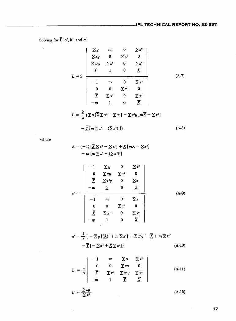
Solving for L, a', b', and C':

Ey M

0

x2y X2

1 E =

o 1x2

X2 0

o :x

oX(A-7)

where

—1 in 0 1 X2

0 0 2 r2 0

K E X2 0

—m 1 0 X

+Y[mx _(X2)2])

(A-8)

= (-1)[x - X} +[mX - X2]

- m [M E X - (I X2)2]

—1 >y 0 >X2

o xy E X2 0

X x2y 0 x4

—m Y 0 X

a' = (A-9)

—1 m 0 x2

o 0 2 X2 0 Xz 0 :x

—m 1 0

x4 +x2 ]) (A-b)

—1 m Eyx2

0 xy 0(A-il)

. x2 x2y

—m 1 Y X

b' = (A-12)

17


I —1 m 0 Ey

0 0 E X2 >.Xy I

C' = -: " 0 2

(A-13)

—ml 0

+ Y[— x2 +tmXJ} (A-14)

The probable errors of the data points are

[y + (L/2) - a' - b'x - C'X2]

PER, = 0.6745 _° (rn + 1)/2

2 )½ /

(A-15) [y - (L/2) - a' - b'x C'X2]2

PPE, = 0.6745 /

(m -

)½

S

To derive a probable error of the mean insertion loss L, (A-8) is written in the form

= -- { ay + 2 ay) (A-16)

This is expanded in terms of a, the coefficients of the data points, as

L={aiyi+a3y3+ } +{a2y2+a4y4+ ) (A-17)

Substituting (A-8) into (A-16) and (A-17) and summing over the data points gives expressions for the odd and even coefficients:

a2 =-{[X2 + (m - l)x - (X2)2]2(m1)

_2[x2 +(m — lX4 - (X2)2} [rn— E X2] 2 X2 + [Mj^

(A-18)

a2 = 4 ^ []^ 2 X2 — (M + X4 + (I X2)2]2 M

_2x2_ (m+l)x4 +(x2 ) 2 ] [_X2]X2 + [m_x2]2x4}

(A-19)

The probable error of the mean insertion loss is then

PE ([PE,]2E a2 + [PEye]2 2 a2)½ (A-20)

18


APPENDIX B

Computer Programs

These two programs, one for the first-order analysis, the other for the second-order analysis, are written in Fortran for an IBM 1620 Computer. Symbol m is the total number of observed points R, and each program can handle a maximum of m = 50. The values of R and M

are the inputs required. The output of each program

prints the observed points R; the ratios y converted to db; the individual insertion-loss measurement L; the straight line and parabola constants a, b, and a', b', C'; the prob-able errors of the odd and even data points, PE, PE,,;

the mean insertion losses L; and the probable errors of the mean insertion loss, PEE.

I. FIRST-ORDER ANALYSIS

1 FORMAT )1H1,48HINSERTION LOSS DATA REDUCTION,1ST ORDER ANALYSIS) 2 FORMAT) 1HO,6X1HR,12X1HY,15XIHE,14X21IL1) 3 FORMAT ( iN ,F9.6,5XEI1.5,5XE11.5,5XEE1.5) 5 FORMAT II5) 6 FORMAT (Flo .0) 7 FORMAT (1HO,4X2HAE1I.5,5X2H8=Eii.5) 8 FORMAT)))) ,4X,5HPEYO=Ei1.5,3X5IIPEYEEI1.5) 9 FORMAT)IH ,4X2HLEii.5,6X4HPELE11.)

12 FORMAT)1H ,F9.6,2)AX,Ei).5)) DIPENSION R)50),Y)50),X)50) ,E)50),EL1)50)

25 READ 5,M EM =M N M- 1 PRINT 1 PRINT 2 SUME=O.O SUMD=O .0 SLIMXY=O.O SUMXQO.O SEOQO.O SEEQ=O .0 00 30 11,M READ6,R)I)

30 Y)I)=-20.O.0.43429LOGF(R)I)) DO 32 11,N,2

32 EL1(I )Y(I+1)-Y(I ) DO 33 i'2,M,2

33 ELI( I )Y)I )-Y(I1) 00 35 1=2,11,2

35 SUME= SUM EY)I) LE= (2.1)

EM-i")*SUM' DO 40 11,11,2 40 SUMO=SUMOY(I)

ELO=(2./)EM+1.))SUMO ELELE-ELO A(ELE+E1O)/2. XMIN=)-(EM-1.0)/2.0)-)i.D) 0045 I=1,M X(I )=XMINi. EM IN=X)I( O YX II .)I) XQ=X) I

) (

Y2 .

SUMXYSUMXY*XY 45 SUMXQSUMXQXQ

BSUMXY/SL(MXQ DO 50 I=1,M,2 ElI )=Y)I)*EL/2.-A-8X( I) EOQ=E)I)..2

50 S8OQSE0QEO0 DO 5512,M,2 Eli )Y(I (-A-B.X)I )-EL/2. EEQE(I)'.2

55 SEE Q=SEEQEEQ PEYO=.6745.SQRTF)SEOQ/HEM.1.)/2.)) PEYE=.6745.SORTF(SEEQ/((EM-1.)/2.() Pi=)2./(EM.1 I )*PEYIJ.2 P2=)2.0/IEMi-.D( l.PEYE..2 PEL=SQRTF(Fi+F2) DO 60 1=1,6

60 PRINT 3,R(i),Y1i),E(I(,EL1(I) PRINT 12,R(M),Y(M),E)M( PRINT 7,8,0 PRINT 8,PEYO,PEYE PRINT 9,EL,PEL GO TO 25 END

19


II SECOND-ORDER ANALYSIS

I FORMAT)1HI.48HINSERTION LOSS DATA REDUCTION.2ND ORDER ANALYSIS) 2 FORMAT )IHO,EXYHR,9X1HY,I3XIHE,13X2HL1 I 3 FORMAT (1H ,4)4X,E1I.5)) 4 FORMAT(15) 5 FORMAT)F10.0) I, FORMAT) IHO,2MAETJ.5,3X2HBEII.5.3X2HCEII.5) 7 FORMAT )IH ,5HPEYO=EIl.5,SX5HPFYEE!1.5) 8 FORMAT( 1H ,2HLEI1.5,6X4NFELE1I.5) 9 FORMAT )IH .3iYX.Eil.5))

DIMENSION R)50),Y)50), X)50), E)50), ELI(50) 25 REAO4,M

PRINT 1 PR) NT 2 EM =M N=M-1 0035 I=1,M READ 5,R(l)

35 Y)I)=-2O.00.43429LOGF)N)I)) 0=0.0 F =0.0 G0.0 - H-0:0 P=O .0 5=0.0 U=O.O v=0.O w=0.O E00.O FE 0. 0 0040 11.N,2 - FL))!) Y) 1*1 )-Y) I)

40 CONTINUE 0042 I=2,N,2 ELI))) Y) I) -V(I1)

42 CONTINUE D04411 ,M,2 OlY)I)

64 CONTINUE 5046 I2,N.2 FF+V)I)

46 CONTINUE IC)-M+1)/2-1 0048) 1 .M 0)! )IC+I

48 CONTINUE 0050 I1,M,2 G0+)X)) I "2

50 CONTINUE 0052 I2,N,2 HH+ ) X)1)) "2

52 CONTINUE 0054 I1,M PP+)X) I) 14

54 CONTINUE DELTA=-(G-H)*)0+N)+P+)C--I-4))EM)G-H)-(G+H))-EM)EMP)G+K)*2) 005611,M 55+V) I ) XI 1)) "2

56 CONTINUE 0T )2./DELTA 4) (O+F )( )G-H))G+N)-Pl-S( EM • )G-H)-(0+l-)) I 1+10-F)) EM'P- ) G*H ) "2)) 0058 11.M 11U*X) I )V) I)

58 CONTINUE 0A11./0ELTA)) )O+F)) )0-H) . .2-EM4P)+S(1fG+EM)0 6 H) I 1-lO-F)I-P+)G-HI)0*H) I

BU/)D+H) 0C) i./DELTA)1 (O+F)(H-0*EM(0+H) )-S)EM"2-1. 1+)0-F))-G-H+EM')0-H) DOC I1

.M,2

El Il=Y)I)+T/2.-A-8*X)I)-C)X))) )2 EOE)I)"2 +EO

60 CONTINUE 0062 12,N.2 E(!) =311) -T/2.ABX) I )-C (X)!)) "2 EEEII)2 *EE

• 62 CONTINUE PEYO=.6745SORTF lEO/I )EM+1.I/2.) PEVE=.6745S0RTF) EE/ ))EM- 1.)/2.)) 0064 1=1

'2 64 .CONTINUE

• 0066 I2.N.2 WW+) X)I)) "4

66 CONTINUE OAA( )EM+1.)/2. )( ))0H)10+H)*)EM1. )P-)G*H)2)"2) 1-12. ).G)EM)0-H)-)0,H) )) )G.H))G-H)*)EM-1. )P-)G+H)"2) 2+V*) I EM) 0-H)-) 5*1-f lI"2 I OBBUEMi.)/2.)*I))0H))0+H))EM1.)P+)G*H)*2)"2) 1_)2.)*H)EM*)G_H)_(G*H))))5+N)*)G_H)_)EM_1.)*P_)01-f)**2) 2+W -H)-)G*H) l2) PEL=2.SORTF)AA) )PEYO/DELTA)2)+B8) (PEYE/DELTA)"2) ) 0068 11,N PRINT 3,R) I) ,Y) II ,E( I) ,ELI ) II

68 CONTINUE PRINT 9,RIMI,Y)M) ,E)M) PRINT 6.A,8,C PRINT 7,PEYO.PEVE PRINT 8,T,PEL GO TO 25 END

- 20

a precision dc-potentiometer microwave - nasa · a precision dc-potentiometer microwave - ......

Documents