At

SA

a

ARRA

KCHMNPT

1

asoscnpl

0d

Fisheries Research 107 (2011) 1–13

Contents lists available at ScienceDirect

Fisheries Research

journa l homepage: www.e lsev ier .com/ locate / f i shres

practical guide to statistical methods for comparing means fromwo-stage sampling

usan J. Picquelle, Kathryn L. Mier ∗

laska Fisheries Science Center, National Marine Fisheries Service, National Oceanic and Atmospheric Administration, 7600 Sand Point Way NE, Seattle, WA 98115, USA

r t i c l e i n f o

rticle history:eceived 11 February 2010eceived in revised form 14 June 2010ccepted 9 September 2010

eywords:luster samplingierarchical designixed modelested ANOVAseudoreplicationwo-staged sampling

a b s t r a c t

Two-staged sampling is the method of sampling populations that occur naturally in groups and is commonin ecological field studies. This sampling method requires special statistical analyses that account for thissample structure. We present and compare several analytical methods for comparing means from two-stage sampling: (1) simple ANOVA ignoring sample structure, (2) unit means ANOVA, (3) Nested MixedANOVA, (4) restricted maximum likelihood (REML) Nested Mixed analysis, and (5) REML Nested Mixedanalysis with heteroscedasticity.

We consider a fisheries survey example where the independent sampling units are subsampled (i.e.,hauls are the sampling unit and fish are subsampled from hauls). To evaluate the five analytical methods,we simulated 1000 samples of fish lengths subsampled from hauls in two regions with various levelsof: (1) differences between the region means, (2) unbalance among numbers of hauls within regionsand numbers of fish within hauls, and (3) heteroscedasticity. For each simulated sample, we tested fora difference in mean lengths between regions using each of the five methods. The inappropriate, simpleANOVA that ignored the sample structure resulted in grossly inflated Type I errors (rejecting a truenull hypothesis of no difference in the means). We labeled this analysis the Pseudoreplication ANOVAbased on the term “pseudoreplication” that describes the error of using a statistical analysis that assumesindependence among observations when in fact the measurements are correlated. The result of this erroris artificially inflated degrees of freedom, giving the illusion of having a more powerful test than the datasupport.

The other four analyses performed well when the data were balanced and homoscedastic. When there

were unequal numbers of fish per haul, the REML Nested Mixed analyses and the Unit Means ANOVAperformed best. The Unequal-Variance REML Nested Mixed analysis showed clear benefit in the presenceof heteroscedasticity and unbalance in hauls. For the REML Nested Mixed analysis, we compared threesoftware packages, S-PLUS, SAS, and SYSTAT.

A second simulation that compared samples with varying ratios of among-haul to among-fish vari-ance components showed that the Pseudoreplication ANOVA was only appropriate when the haul effect

yielded a p-value >0.50.

. Introduction

Two-stage sampling is a common practice in fisheries surveys,s well as many other disciplines. In two-stage sampling, the firsttage refers to the primary sampling unit which is a cluster ofbjects, followed by a second stage where individual objects, orub-units, are subsampled (or completely enumerated) from the

luster (Cochran, 1977). A cluster, or primary sampling unit, is aatural grouping of objects that may have similar attributes. Exam-les of this include fish (sub-units) caught in a trawl net (cluster),

eaves (sub-unit) on a tree (cluster), and seabirds (sub-unit) in a

∗ Corresponding author. Tel.: +1 206 526 4276; fax: +1 206 526 6723.E-mail address: Kathy.Mier@noaa.gov (K.L. Mier).

165-7836/$ – see front matter. Published by Elsevier B.V.oi:10.1016/j.fishres.2010.09.009

Published by Elsevier B.V.

nesting colony (cluster). This sampling scheme is a form of multi-level sampling (Lehtonen and Pahkinen, 2004) and is also referredto as hierarchical (Raudenbush and Bryk, 2002) or nested sampling.This paper focuses on two-stage sampling; however, the methodsdiscussed here also apply to three-stage or higher levels of hierar-chical sampling. The example of two-stage sampling that we usethroughout this paper is the comparison of mean length of fish intwo geographic regions, where fish are caught in a trawl net atseveral locations within each region, and then the catch at eachlocation is subsampled for individual length measurements.

Sampling structure must be accounted for in the statistical anal-ysis of the resulting data, and the primary goal of this paper isto compare alternate analytical methods. A two-stage samplingstructure requires special handling because the way the data arecollected often leads to the lack of independence among the obser-

2 heries

vaafiisoptlocbtfic

ssopsmHPsIw(

dotroct

naodacqo(ptue2suriwoulca

ite

S.J. Picquelle, K.L. Mier / Fis

ations. In fisheries research, one frequently wants to measurettributes of individual fish in the field, for example, length, weight,ge, stomach content, or otolith measurements. However, for mostsh populations, it is impractical to collect a random sample of

ndividual fish in one sampling stage. Instead, volumes of water areampled with nets catching a cluster of many fish, and some or allf the fish in this cluster are measured. Because fish tend to occur inroximity of other similar fish of the same species, either because ofheir schooling behavior or because the local habitat attracts simi-ar fish, sampling a cluster of fish by a net usually results in a samplef fish that are similar to each other. So, simply by virtue of beingaught in the same net, the fish are not independent observations,ut rather correlated. For example, in measuring fish length, fishend to aggregate with other fish of similar size, so measuring onesh from a net provides information on the lengths of the other fishaught in the same net.

A secondary goal of this paper is to show that ignoring theampling structure in the analysis results in erroneous conclu-ions. Specifically, in two-stage sampling, the error of ignoring thatbjects were sampled in clusters and treating the objects as a sim-le random sample is a form of pseudoreplication (Hurlbert, 1984),pecifically sacrificial pseudoreplication, which has been well docu-ented, and has been a common mistake made by researchers (e.g.,airston, 1989; Heffner et al., 1996; Millar and Anderson, 2004).seudoreplication has also been described in social and medicalciences, and in education, although they may use a different term.n clustered randomized trials, it is called a “mismatch” problem

here the units of assignment do not match the units of analysisHedges, 2007; Institute of Educational Sciences, 2007).

The analytical methods examined in this paper avoid pseu-oreplication by using either aggregated data (using cluster means)r using hierarchical (or nested) analysis. In contrast, the approachhat is often used in the mismatch literature referenced above cor-ects pseudoreplication by modifying the test statistics and degreesf freedom, based on the intra-class correlation coefficient withinlusters (Hedges, 2007). We advocate methods that avoid ratherhan correct for pseudoreplication in the statistical analysis.

Before proceeding, we present some necessary statistical termi-ology. A “primary sampling unit” is defined as an element within“sampling frame” that is sampled and is statistically independentf other sampling units within the frame. The sampling frame isefined as the collection of all elements (primary sampling units)ccessible for sampling in the population of interest. In ecologi-al sampling, the primary unit may be a quadrat from all possibleuadrats within a geographic area (frame). Examples are a parcelf land (quadrat) in a watershed (frame), or a column of waterquadrat) in a body of water (frame). In two-stage sampling, therimary sampling units contain sub-units and measurements areaken on individual sub-units. In experimental contexts, the sub-nits within an experimental unit are sometimes referred to asvaluation units (Hurlbert and White, 1993; Kozlov and Hurlbert,006; Urquhart, 1981). One such example is the diameters (mea-urement) of trees (sub-unit) in a land parcel (primary samplingnit or quadrat) where the watershed (frame) is separated into sub-egions (factor of interest). The example in fisheries that we employn this paper is the lengths (measurement) of fish (sub-unit) in the

ater column (primary sampling unit or quadrat) where the bodyf water (frame) is separated into sub-regions (factor). The individ-al fish are not independent observations from the population. The

ack of independence inherent in hierarchical sampling design pre-ludes the use of simple statistics to estimate means and variances,

nd to test hypotheses.

Hierarchical measurements occur in both field sampling andn laboratory experiments. Manipulative experiments, as opposedo field sampling, are analogous to two-stage sampling if thexperimental unit contains evaluation units receiving the same

Research 107 (2011) 1–13

treatment; here, the experimental unit is analogous to the primarysampling unit, the evaluation units are the sub-units, and the treat-ment is analogous to the factor of interest. For example, a treatmentis applied to a tank of fish (experimental unit, the independentobservations) and measurements are made on the individual fishin the tank (sub-units, the correlated observations). Of course morethan two stages of sampling may be applied. For example, a thirdlevel would be where multiple observations are then made on theindividual fish, such as multiple samples of muscle tissue takenfrom each fish for measurement of pollutant levels. For the sake ofsimplicity, we focus on just two levels; however, our conclusionscan be extended to higher level structures.

There are several other special cases of hierarchical samplingprotocols that are sometimes confused with the multi-stage sam-pling that we examine in this study. To avoid confusion, we listsome of these in Appendix H.

In this paper, we focus on two-stage sampling as it applies to sur-veys of fish populations. We simulated samples based on observedpopulation parameters from a well-studied fish population (i.e.,a population of juvenile walleye pollock, Theragra chalcogramma)in the Gulf of Alaska (Kendall et al., 1996). Based on these sim-ulated samples, we examined the probability of rejecting a truenull hypothesis (commonly labeled as a Type I error rate = ˛) andthe probability of not rejecting a false null hypothesis (commonlylabeled as a Type II error rate = ˇ) to evaluate the performance offive different analyses for two-stage sampled data. These analy-ses included two standard non-hierarchical analysis of variance(ANOVA) (one using a measurement per fish and one using themean measurement per haul) and three analyses that correctlyincorporate a nested structure in the data using both ordinary leastsquares (OLS) and restricted maximum likelihood (REML) (West etal., 2007) methods.

Our goals were to determine: (1) the most accurate and pow-erful analyses, (2) how different degrees of unbalance in both thenumber of sub-units within sampling units and number of sam-pling units within factor levels affect the results, (3) how unequalvariances among the factor levels affect the results, (4) what statis-tical software packages are currently the most appropriate for thisproblem, and (5) under what conditions two-stage sampling maybe ignored in the analysis, if at all. We also wanted to emphasizethe dangers of pseudoreplication, particularly in fisheries science,even though these have already been well publicized, especially inthe context of manipulative experiments (Hurlbert, 1984; Hurlbertand White, 1993).

2. Methods

We compared analytical methods for testing the hypothesis ofequal means for a hierarchical design, specifically two-stage sam-pled data, where the first stage consists of primary sampling unitswithin a factor level, each containing many sub-units, and the sec-ond stage consists of subsampling the sub-units. In addition tothe complexity of a hierarchical design due to the lack of inde-pendence among the data, another layer of complexity is addedwhen the sampling (or experimental) units contain different num-bers of sub-units. In the laboratory, equal sample sizes are routinelyattempted, but rarely attained. For the example of fish subsampledfrom tanks, fish invariably die during the experiment or some mea-surements are lost, resulting in unequal numbers of sub-units perexperimental unit. In addition, entire tanks might fail, resulting in

unequal numbers of experimental units per treatment level. In thefield, equal number of sub-units per sampling unit (e.g., numbersof fish per haul where measurements are taken on individual fish)are not expected, and can vary by several orders of magnitude, evenafter adjusting for the varying amounts of water sampled (i.e., sam-

S.J. Picquelle, K.L. Mier / Fisheries Research 107 (2011) 1–13 3

Table 1List of conditions that formed the 120 scenarios used to simulate sampled populations: 3 regional effects × 5 levels of haul unbalance × 4 levels of fish unbalance × 2 levelsof heteroscedasticity = 120 scenarios.

Level Region effects Mean in Region 1 Mean in Region 2

1 Equal 71.6 71.62 Differ by 1 SD 71.6 78.23 Differ by 2 SD 71.6 84.8

Haul unbalance (%) # Hauls in Region 1 # Hauls in Region 2

1 0 15 152 20 12 183 40 9 214 60 6 245 80 3 27

Fish unbalance # Hauls with # fish per haul # Hauls with # fish per haul

1 Equal 30 hauls with 25 fish each2 Some hauls with 1 fish 24 hauls with 31 fish each 6 hauls with 1 fish each3 Most hauls with few fish 20 hauls with 5 fish each 10 hauls with 65 fish each4 Most hauls with many fish 20 hauls with 35 fish each 10 hauls with 5 fish each

Variability within regions SD in Region 1 SD in Region 2

6.4.

ptawmathbfh(btarc

sreaHwwl

b(iilc

2

e(rt

1 Equal2 Unequal

ling effort). Not only do the numbers of fish per haul vary, buthe numbers of hauls per factor level (e.g., year or region or gear)lso often vary. Frequently, in retrospective studies, the samplingas not originally designed for the new purpose or analysis. Thisight result in the numbers of hauls per factor level being unequal

nd a random variable because they were not fixed for each fac-or level a priori; this is comparable to post-stratification, whichas its own issues (Cochran, 1977). Another case where the num-ers of hauls per factor level might differ is stratified sampling;requently the numbers of hauls are proportional to the among-aul standard deviations or mean abundances within each stratume.g., Weinberg et al., 2002). This degree of unbalance in both num-ers of hauls per region and numbers of fish per haul requireshe use of approximations for the variance components in a hier-rchical ANOVA (Satterthwaite, 1946; Sokal and Rohlf, 1995) orestricted maximum likelihood (REML) estimation of the varianceomponents (Laird and Ware, 1982; Pinheiro and Bates, 2000).

From here forward, we will follow the example of a fisheriesurvey where fish are subsampled from hauls; hence, instead ofeferring to sub-units and units we will refer to fish and hauls. Ourxample is a comparison of mean lengths of fish from two regionsnd the null hypothesis is that there is no difference in mean length.auls were sampled from the sampling frame of all possible haulsithin each region using simple random sampling. Individual fishere then subsampled from the catch of fish in each haul and their

engths were measured, again using simple random sampling.The analytical methods to test the null hypothesis were assessed

y comparing their Type I (rejecting a true hypothesis) and Type IIfailing to reject a false hypothesis) error rates, and their accuracyn estimating variance components, i.e., partitioning the variabilityn the data into haul variance and fish variance. We used simu-ated data representing a wide range of sampling and populationonditions to perform the comparisons (see below).

.1. Simulation

We based our simulations on observed lengths of juvenile wall-ye pollock collected by midwater trawling in the Gulf of AlaskaGOA) (Wilson et al., 2006). Samples of fish lengths within eachegion were simulated from normal probability distributions usinghe random normal generator within the function “rnorm” in

59 6.5939 8.78

SPLUS, version 7.0. The GOA data yielded the parameters for thenormal distributions (Table 1). Rather than simulating a popula-tion and then sampling from it, we simulated the samples directly(see details in Appendix A).

We investigated 120 different scenarios (i.e., combinations ofseveral characteristics of populations and sampling designs) sim-ulating 1000 samples for each scenario (Table 1). Each of the 1000samples from all 120 scenarios consisted of two regions, 30 hauls,and a total of 750 fish lengths. To examine Type I error rates (˛) andthe power (1 − ˇ) of the tests, we simulated samples for scenar-ios with three values for region effect; equal mean lengths in eachregion (null hypothesis is true and rejecting the null hypothesis isa Type I error), region means differing by one standard deviationand differing by two standard deviations (null hypothesis is falseand failing to reject the null hypothesis is a Type II error).

Of primary interest is how the various analytical methods wereaffected by unequal numbers of fish per haul and unequal numbersof hauls per region (unbalanced design), and unequal among-haulvariance between regions (heteroscedasticity). To investigate theeffect of unbalance in numbers of hauls among regions in the sam-ple design, we created scenarios where the number of hauls in oneregion differed from the other by 0% (balanced), 20% (40% of haulsin one region vs. 60% in the other region), 40% (30% vs. 70%), 60%(20% vs. 80%), and 80% (10% vs. 90%). In all haul allocation schemes,the total number of hauls sampled remained the same. For unbal-ance in numbers of fish among hauls, we looked at four allocationschemes, (1) all hauls had an equal number of fish, (2) some haulshad a single fish, (3) most hauls had few fish and (4) most hauls hadmany fish (Table 1). In all fish allocation schemes, the total numberof fish sampled remained the same.

To examine heteroscedasticity, we examined all scenariosdescribed above with both equal and unequal among-haul vari-ances for each region. For the unequal variance scenarios,among-haul variance in one region was four times that of the otherregion. One valid reason for an unbalanced design is to base thenumber of samples on the variability within a factor level. Hence,

for the unequal variance, we put the greater number of hauls in theregion with the higher among-haul variance. Forming all possiblecombinations of these factors led to 120 unique scenarios, i.e., 3(region effects) × 5 (unbalance in hauls) × 4 (unbalance in fish) × 2(heteroscedasticity) (Table 1).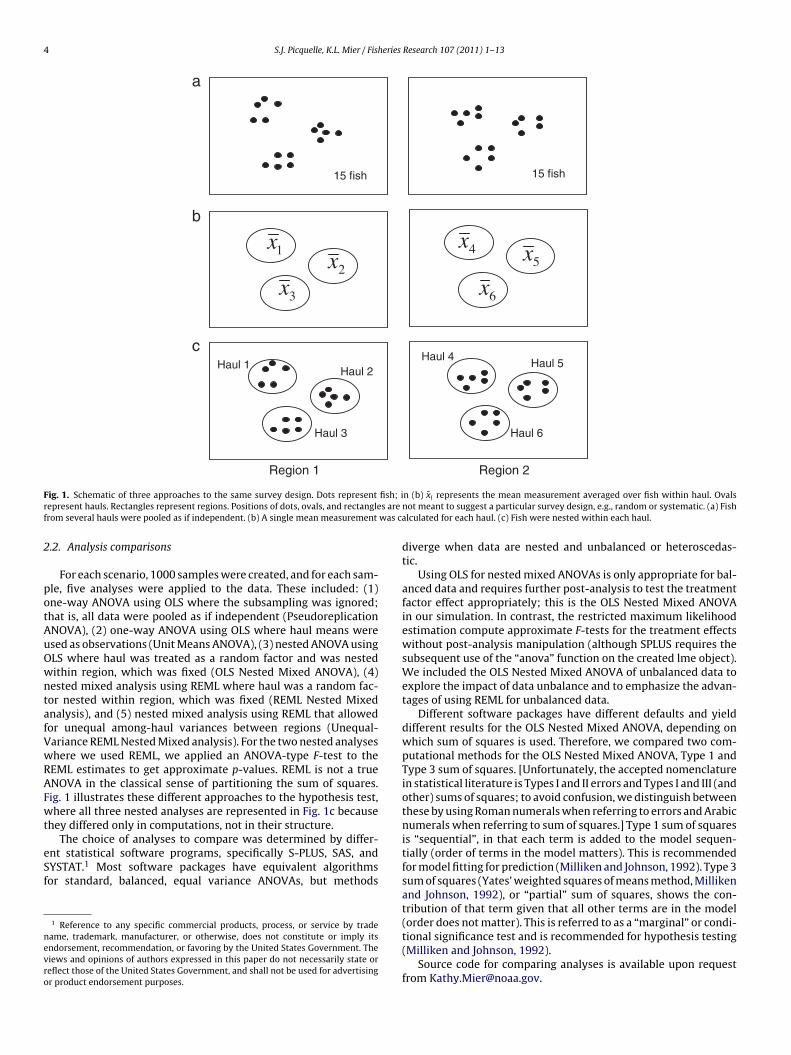

4 S.J. Picquelle, K.L. Mier / Fisheries Research 107 (2011) 1–13

Region 1 Region 2

1x2x

3x

4x5x

6x

Haul 1Haul 2

6luaH3luaH

Haul 5Haul 4

15 fish

a

b

c

15 fish

F fish; ir s aref was c

2

potAuOwntafVwRAFwt

eSf

nevro

ig. 1. Schematic of three approaches to the same survey design. Dots representepresent hauls. Rectangles represent regions. Positions of dots, ovals, and rectanglerom several hauls were pooled as if independent. (b) A single mean measurement

.2. Analysis comparisons

For each scenario, 1000 samples were created, and for each sam-le, five analyses were applied to the data. These included: (1)ne-way ANOVA using OLS where the subsampling was ignored;hat is, all data were pooled as if independent (PseudoreplicationNOVA), (2) one-way ANOVA using OLS where haul means weresed as observations (Unit Means ANOVA), (3) nested ANOVA usingLS where haul was treated as a random factor and was nestedithin region, which was fixed (OLS Nested Mixed ANOVA), (4)ested mixed analysis using REML where haul was a random fac-or nested within region, which was fixed (REML Nested Mixednalysis), and (5) nested mixed analysis using REML that allowedor unequal among-haul variances between regions (Unequal-ariance REML Nested Mixed analysis). For the two nested analyseshere we used REML, we applied an ANOVA-type F-test to theEML estimates to get approximate p-values. REML is not a trueNOVA in the classical sense of partitioning the sum of squares.ig. 1 illustrates these different approaches to the hypothesis test,here all three nested analyses are represented in Fig. 1c because

hey differed only in computations, not in their structure.

The choice of analyses to compare was determined by differ-

nt statistical software programs, specifically S-PLUS, SAS, andYSTAT.1 Most software packages have equivalent algorithmsor standard, balanced, equal variance ANOVAs, but methods

1 Reference to any specific commercial products, process, or service by tradeame, trademark, manufacturer, or otherwise, does not constitute or imply itsndorsement, recommendation, or favoring by the United States Government. Theiews and opinions of authors expressed in this paper do not necessarily state oreflect those of the United States Government, and shall not be used for advertisingr product endorsement purposes.

n (b) x̄i represents the mean measurement averaged over fish within haul. Ovalsnot meant to suggest a particular survey design, e.g., random or systematic. (a) Fishalculated for each haul. (c) Fish were nested within each haul.

diverge when data are nested and unbalanced or heteroscedas-tic.

Using OLS for nested mixed ANOVAs is only appropriate for bal-anced data and requires further post-analysis to test the treatmentfactor effect appropriately; this is the OLS Nested Mixed ANOVAin our simulation. In contrast, the restricted maximum likelihoodestimation compute approximate F-tests for the treatment effectswithout post-analysis manipulation (although SPLUS requires thesubsequent use of the “anova” function on the created lme object).We included the OLS Nested Mixed ANOVA of unbalanced data toexplore the impact of data unbalance and to emphasize the advan-tages of using REML for unbalanced data.

Different software packages have different defaults and yielddifferent results for the OLS Nested Mixed ANOVA, depending onwhich sum of squares is used. Therefore, we compared two com-putational methods for the OLS Nested Mixed ANOVA, Type 1 andType 3 sum of squares. [Unfortunately, the accepted nomenclaturein statistical literature is Types I and II errors and Types I and III (andother) sums of squares; to avoid confusion, we distinguish betweenthese by using Roman numerals when referring to errors and Arabicnumerals when referring to sum of squares.] Type 1 sum of squaresis “sequential”, in that each term is added to the model sequen-tially (order of terms in the model matters). This is recommendedfor model fitting for prediction (Milliken and Johnson, 1992). Type 3sum of squares (Yates’ weighted squares of means method, Millikenand Johnson, 1992), or “partial” sum of squares, shows the con-tribution of that term given that all other terms are in the model

(order does not matter). This is referred to as a “marginal” or condi-tional significance test and is recommended for hypothesis testing(Milliken and Johnson, 1992).

Source code for comparing analyses is available upon requestfrom Kathy.Mier@noaa.gov.

eries

2

yhtcrScrwi

IrmisassvabpttwptstespIhwt1

2

cmAwswuturr

2

scsi

S.J. Picquelle, K.L. Mier / Fish

.3. Type I and Type II errors

The primary criterion that we used to determine the best anal-sis was to compare the rate that the analysis rejected a trueypothesis (Type I error) to the specified ˛ for the hypothesisest of no difference between region means. Type I errors wereounted from all 1000 samples from each of the 40 scenarios whereegion means were equal and compared among the five analyses.imilarly, Type II errors (failing to reject a false hypothesis) wereounted from all 1000 samples from each of the scenarios whereegion means differed. The tabulated Type I and Type II error ratesere then compared among the five analyses. For these compar-

sons, we set ˛ = 0.05.Note that ˛ = 0.05 is an arbitrary test criterion and basing Type

and Type II error rates on arbitrary significance levels are directlyelevant only to hypothesis testing. In practice, we highly recom-end reporting p-values as evidence in support of a hypothesis

nstead of accepting or rejecting a hypothesis based on arbitraryignificance levels. We use Type I and Type II error rates here fordifferent purpose—to evaluate the accuracy of different analy-

es, i.e., how close is the computed p-value associated with the testtatistic from the analysis to the actual probability of observing thatalue of the statistic. Type I error rate compares the nominal prob-bility of ˛ = 0.05 with the actual probability, which we estimatedy the observed proportion of 1000 simulations that resulted in arobability of 0.05 or smaller. If the observed Type I error rate, i.e.,he actual probability, is close to the nominal probability, then theest is accurate. A more rigorous measure of the accuracy of the testsould be to compute the observed p-values for a variety of nominalrobabilities and then compare these to an F-distribution. However,he probabilities that are of greatest interest are the small values,o we restricted our comparisons to a single nominal probability,he ˛ value of 0.05. We chose this criterion because, traditionally incology, as opposed to quality control in manufacturing, hypothe-is testing has usually emphasized controlling and minimizing therobability (˛) of incorrectly rejecting a true null hypothesis (Typeerror), rather than the probability (ˇ) of failing to reject a false nullypothesis (Type II error). However, the frequency of Type II errorsas included in this evaluation as this is indicative of the power of

he test (i.e., the ability to correctly reject a false null hypothesis, or− ˇ).

.4. Variance components

Another measure of performance of the five analyses was toompare the estimated variance components from each of theethods to those used to simulate the sample data (Appendicesand B). That is, we specified a variance about the haul meanshen simulating them and consequently, a component of the mean

quare for haul is an estimate of this specified variance. Similarly,e specified a variance for the individual fish lengths when sim-lating them and the mean square error (MSE) is an estimate ofhat variance. We focused on the variance among primary samplingnits within factor level (i.e., variance among haul means withinegion) because this is critical for testing for differences amongegion means. See Appendix B for details.

.5. Software comparisons

The three software packages (S-PLUS, SAS, and SYSTAT) differ inubtle computational details of the nested analyses. The softwareode for the REML Nested Mixed analyses is challenging, hence wehow it in Appendix C. The details of the software comparisons aren Appendix D.

Research 107 (2011) 1–13 5

2.6. Pooling

We conducted a second simulation study to elucidate theconditions that might allow pooling the two sampling stages(and corresponding sums of squares) without compromising thevalidity of the hypothesis tests. Hurlbert (2004) labeled this “test-qualified pseudoreplication”. In other words, when is it acceptable,if ever, to ignore the nested structure of the sampling designand treat all the subsampled individuals (sub-units, in our exam-ple, fish) as independent observations? Details of this poolingsimulation and brief review of the literature are in AppendixE.

3. Results

3.1. Type I errors

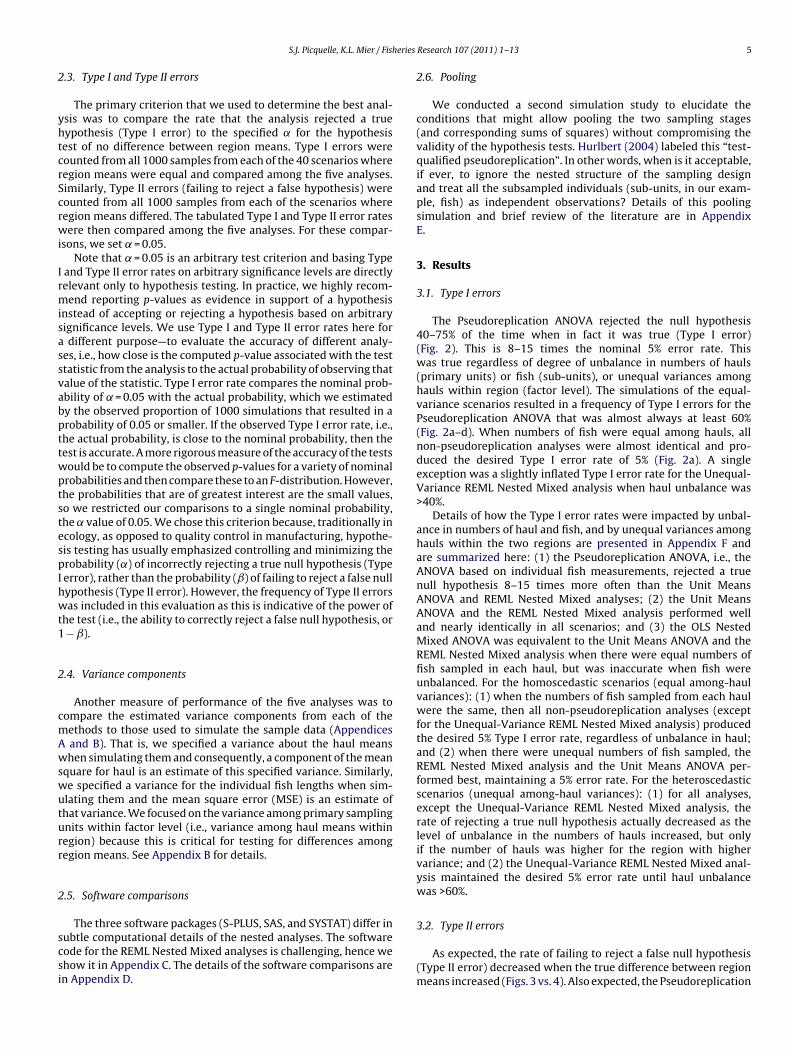
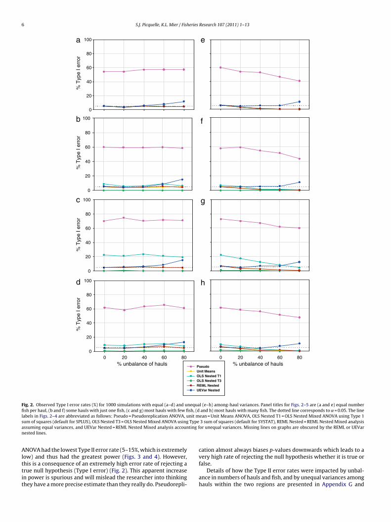
The Pseudoreplication ANOVA rejected the null hypothesis40–75% of the time when in fact it was true (Type I error)(Fig. 2). This is 8–15 times the nominal 5% error rate. Thiswas true regardless of degree of unbalance in numbers of hauls(primary units) or fish (sub-units), or unequal variances amonghauls within region (factor level). The simulations of the equal-variance scenarios resulted in a frequency of Type I errors for thePseudoreplication ANOVA that was almost always at least 60%(Fig. 2a–d). When numbers of fish were equal among hauls, allnon-pseudoreplication analyses were almost identical and pro-duced the desired Type I error rate of 5% (Fig. 2a). A singleexception was a slightly inflated Type I error rate for the Unequal-Variance REML Nested Mixed analysis when haul unbalance was>40%.

Details of how the Type I error rates were impacted by unbal-ance in numbers of haul and fish, and by unequal variances amonghauls within the two regions are presented in Appendix F andare summarized here: (1) the Pseudoreplication ANOVA, i.e., theANOVA based on individual fish measurements, rejected a truenull hypothesis 8–15 times more often than the Unit MeansANOVA and REML Nested Mixed analyses; (2) the Unit MeansANOVA and the REML Nested Mixed analysis performed welland nearly identically in all scenarios; and (3) the OLS NestedMixed ANOVA was equivalent to the Unit Means ANOVA and theREML Nested Mixed analysis when there were equal numbers offish sampled in each haul, but was inaccurate when fish wereunbalanced. For the homoscedastic scenarios (equal among-haulvariances): (1) when the numbers of fish sampled from each haulwere the same, then all non-pseudoreplication analyses (exceptfor the Unequal-Variance REML Nested Mixed analysis) producedthe desired 5% Type I error rate, regardless of unbalance in haul;and (2) when there were unequal numbers of fish sampled, theREML Nested Mixed analysis and the Unit Means ANOVA per-formed best, maintaining a 5% error rate. For the heteroscedasticscenarios (unequal among-haul variances): (1) for all analyses,except the Unequal-Variance REML Nested Mixed analysis, therate of rejecting a true null hypothesis actually decreased as thelevel of unbalance in the numbers of hauls increased, but onlyif the number of hauls was higher for the region with highervariance; and (2) the Unequal-Variance REML Nested Mixed anal-ysis maintained the desired 5% error rate until haul unbalancewas >60%.

3.2. Type II errors

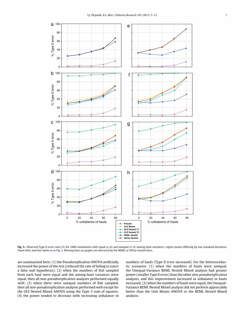
As expected, the rate of failing to reject a false null hypothesis(Type II error) decreased when the true difference between regionmeans increased (Figs. 3 vs. 4). Also expected, the Pseudoreplication

6 S.J. Picquelle, K.L. Mier / Fisheries Research 107 (2011) 1–13

% unbalance of hauls806040200

% T

ype

I err

or

0

20

40

60

80

100

% T

ype

I err

or

0

20

40

60

80

100

% T

ype

I err

or

0

20

40

60

80

100

% T

ype

I err

or

0

20

40

60

80

100a e

f

g

h

b

c

d

PseudoUnit MeansOLS Nested T1OLS Nested T3REML NestedUEVar Nested

% unbalance of hauls806040200

Fig. 2. Observed Type I error rates (%) for 1000 simulations with equal (a–d) and unequal (e–h) among-haul variances. Panel titles for Figs. 2–5 are (a and e) equal numberfish per haul, (b and f) some hauls with just one fish, (c and g) most hauls with few fish, (d and h) most hauls with many fish. The dotted line corresponds to ˛ = 0.05. The linel nit ms Typea ting fn

Alttit

abels in Figs. 2–4 are abbreviated as follows: Pseudo = Pseudoreplication ANOVA, uum of squares (default for SPLUS), OLS Nested T3 = OLS Nested Mixed ANOVA usingssuming equal variances, and UEVar Nested = REML Nested Mixed analysis accounested lines.

NOVA had the lowest Type II error rate (5–15%, which is extremely

ow) and thus had the greatest power (Figs. 3 and 4). However,his is a consequence of an extremely high error rate of rejecting arue null hypothesis (Type I error) (Fig. 2). This apparent increasen power is spurious and will mislead the researcher into thinkinghey have a more precise estimate than they really do. Pseudorepli-

ean = Unit Means ANOVA, OLS Nested T1 = OLS Nested Mixed ANOVA using Type 13 sum of squares (default for SYSTAT), REML Nested = REML Nested Mixed analysisor unequal variances. Missing lines on graphs are obscured by the REML or UEVar

cation almost always biases p-values downwards which leads to a

very high rate of rejecting the null hypothesis whether it is true orfalse.

Details of how the Type II error rates were impacted by unbal-ance in numbers of hauls and fish, and by unequal variances amonghauls within the two regions are presented in Appendix G and

S.J. Picquelle, K.L. Mier / Fisheries Research 107 (2011) 1–13 7

% unbalance of hauls0 20 40 60 80

% unbalance of hauls0 20 40 60 80

% T

ype

II er

ror

0

20

40

60

80

100

% T

ype

II er

ror

0

20

40

60

80

100

PseudoUnit MeansOLS Nested T1OLS Nested T3REML NestedUEVar Nested

% T

ype

II er

ror

0

20

40

60

80

100

% T

ype

II er

ror

0

20

40

60

80

100a

b

c

d

e

f

g

h

F unequP EML

aiafewtt(

ig. 3. Observed Type II error rates (%) for 1000 simulations with equal (a–d) andanel titles and line labels as in Fig. 2. Missing lines on graphs are obscured by the R

re summarized here: (1) the Pseudoreplication ANOVA artificiallyncreased the power of the test (reduced the rate of failing to reject

false null hypothesis); (2) when the numbers of fish sampledrom each haul were equal and the among-haul variances were

qual, then all non-pseudoreplication analyses performed equallyell; (3) when there were unequal numbers of fish sampled,

hen all non-pseudoreplication analyses performed well except forhe OLS Nested Mixed ANOVA using the Type 3 sum of squares;4) the power tended to decrease with increasing unbalance in

al (e–h) among-haul variances; region means differing by one standard deviation.or UEVar nested lines.

numbers of hauls (Type II error increased). For the heteroscedas-tic scenarios: (1) when the numbers of hauls were unequal,the Unequal-Variance REML Nested Mixed analysis had greaterpower (smaller Type II error) than the other non-pseudoreplication

analyses, and this improvement increased as unbalance in haulsincreased; (2) when the numbers of hauls were equal, the Unequal-Variance REML Nested Mixed analysis did not perform appreciablybetter than the Unit Means ANOVA or the REML Nested Mixedanalysis.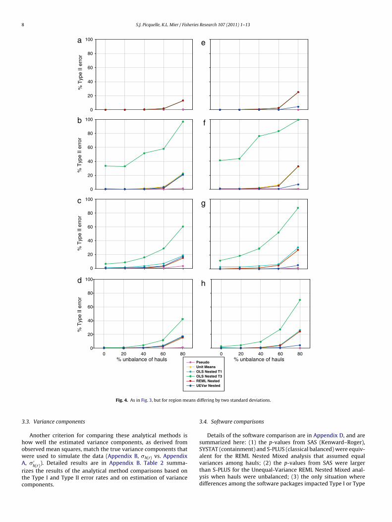

8 S.J. Picquelle, K.L. Mier / Fisheries Research 107 (2011) 1–13

% unbalance of hauls806040200

% unbalance of hauls806040200

% T

ype

II er

ror

0

20

40

60

80

100

% T

ype

II er

ror

0

20

40

60

80

100

PseudoUnit MeansOLS Nested T1OLS Nested T3REML NestedUEVar Nested

% T

ype

II er

ror

0

20

40

60

80

100

% T

ype

II er

ror

0

20

40

60

80

100a

b

c

d

e

f

g

h

ans d

3

howArtc

Fig. 4. As in Fig. 3, but for region me

.3. Variance components

Another criterion for comparing these analytical methods isow well the estimated variance components, as derived frombserved mean squares, match the true variance components that

ere used to simulate the data (Appendix B, �h(r) vs. Appendix, � ′

h(r)). Detailed results are in Appendix B. Table 2 summa-izes the results of the analytical method comparisons based onhe Type I and Type II error rates and on estimation of varianceomponents.

iffering by two standard deviations.

3.4. Software comparisons

Details of the software comparison are in Appendix D, and aresummarized here: (1) the p-values from SAS (Kenward–Roger),SYSTAT (containment) and S-PLUS (classical balanced) were equiv-

alent for the REML Nested Mixed analysis that assumed equalvariances among hauls; (2) the p-values from SAS were largerthan S-PLUS for the Unequal-Variance REML Nested Mixed anal-ysis when hauls were unbalanced; (3) the only situation wheredifferences among the software packages impacted Type I or Type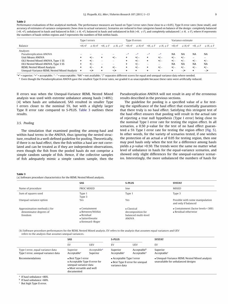

S.J. Picquelle, K.L. Mier / Fisheries Research 107 (2011) 1–13 9

Table 2Performance evaluations of five analytical methods. The performance measures are based on Type I error rates (how close to ˛ = 0.05), Type II error rates (how small), andaccuracy of estimates of variance components (how close to actual variances). Scenarios are reduced to four categories based on balance of the design: completely balanced(=H, =F), unbalanced in hauls and balanced in fish ( /= H, =F), balanced in hauls and unbalanced in fish (=H, /= F), and completely unbalanced ( /= H, /= F), where H representsthe numbers of hauls within regions and F represents the numbers of fish within hauls.

Type I errors Type II errors Variance estimate

Balance =H,=F /= H,=F =H, /= F /= H, /= F =H,=F /= H,=F =H, /= F /= H, /= F =H,=F /= H,=F =H, /= F /= H, /= F

AnalysesPseudoreplication ANOVA − − − − −a −a −a −a NA NA NA NAUnit Means ANOVA + +/− + +/− + +/− + +/− +/− +/− − −OLS Nested Mixed ANOVA, Type 1 SS + +/− − − + +/− + +/− +/− +/− +/− +/−OLS Nested Mixed ANOVA, Type 3 SS + +/− − − + +/− − − NA NA NA NAREML Nested Mixed Analysis + +/− + +/− + +/− + +/− +/− +/− +/− +/−Unequal-Variance REML Nested Mixed Analysis + +/+ + +/+ + + + + + −/+ + −/+

“ es diff, we g

Ia(ITr

3

wtileso

T(

+” = superior; “+” = acceptable; “−” = unacceptable; “NA” = not available; “/” separata Even though the Pseudoreplication ANOVA gave the smallest Type II error rates

I errors was when the Unequal-Variance REML Nested Mixednalysis was used with extreme unbalance among hauls (>40%);4) when hauls are unbalanced, SAS resulted in smaller Typeerrors closer to the nominal 5%, but with a slightly larger

ype II error rate compared to S-PLUS. Table 3 outlines theseesults.

.5. Pooling

The simulation that examined pooling the among-haul andithin-haul terms in the ANOVA, thus ignoring the nested struc-

ure, resulted in a well-defined guideline for pooling. Theoretically,

f there is no haul effect, then the fish within a haul are not corre-ated and can be treated as if they are independent observations,ven though the fish from the pooled hauls do not comprise aimple random sample of fish. Hence, if the collective samplesf fish adequately mimic a simple random sample, then the

able 3a) Software procedure characteristics for the REML Nested Mixed analysis.

SAS

Name of procedure PROC MIXED

Sum of squares used Type 1Type 3

Unequal variance option Yes

Approximation method(s) fordenominator degrees offreedom

• Containment• Between/Within• Residual• Satterthwaite• Kenward–Roger

(b) Software procedure performances for the REML Nested Mixed analysis. EV refers torefers to the analysis that assumes unequal variances.

SAS S-PLUS

EV UEV EV

Type I error, equal variance data Superior Acceptablea SuperiorType I error, unequal variance data Acceptablec Superior Accepta

Recommendations • Best Type I error• Acceptable Type II error forunequal variance data• Most versatile and welldocumented

• Accept

• Best Tyvariance

a If haul unbalance <80%.b If haul unbalance <60%.c But high Type II error.

erent scores for equal and unequal variance data where needed.raded it as unacceptable because these rates were artificially reduced.

Pseudoreplication ANOVA will not result in any of the erroneousresults described in the previous sections.

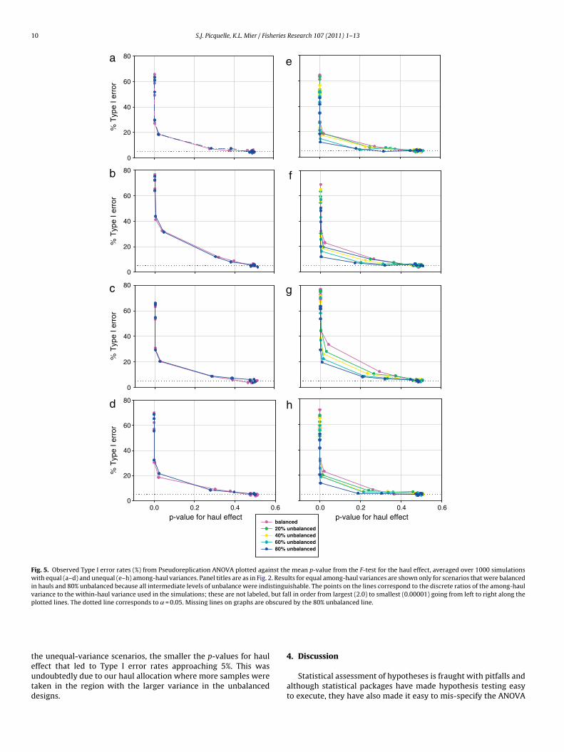
The guideline for pooling is a specified value of ˛ for test-ing the significance of the haul effect that essentially guaranteesthat there truly is no haul effect. Satisfying this stringent test ofthe haul effect ensures that pooling will result in the actual rateof rejecting a true null hypothesis (Type I error) being close tothe nominal Type I error rate for testing the region effect. In allscenarios, a 0.50 p-value for the test of no haul effect guaran-teed a 5% Type I error rate for testing the region effect (Fig. 5).In other words, for the variety of scenarios tested, if one wishesthe protection of an actual ˛ of 0.05 for testing region, then one

may pool hauls only when the test for a difference among haulsyields a p-value >0.50. The trends were the same no matter whatlevel of unbalance in hauls for the equal-variance scenarios, andshowed only slight differences for the unequal-variance scenar-ios. Interestingly, the more unbalanced the numbers of hauls for

S-PLUS SYSTAT

lme MIXED

Type 1 Type 3

Yes Possible with some manipulationand only if balanced

• Classicaldecomposition forbalanced multi-levelANOVA

• Containment (factor levels < 300)• Residual otherwise

the analysis that assumes equal variances and UEV

SYSTAT

UEV EV

Acceptableb Superiorblec Acceptablea Acceptablec

able Type I error • Unequal-Variance REML Nested Mixed analysisunavailable for unbalanced designspe II error for unequal

data

10 S.J. Picquelle, K.L. Mier / Fisheries Research 107 (2011) 1–13

p-value for haul effect0.60.40.20.0

balanced20% unbalanced40% unbalanced60% unbalanced80% unbalanced

p-value for haul effect0.60.40.20.0

% T

ype

I err

or

0

20

40

60

80

% T

ype

I err

or

0

20

40

60

80

% T

ype

I err

or

0

20

40

60

80

% T

ype

I err

or

0

20

40

60

80a

b

c

d

e

f

g

h

Fig. 5. Observed Type I error rates (%) from Pseudoreplication ANOVA plotted against the mean p-value from the F-test for the haul effect, averaged over 1000 simulationswith equal (a–d) and unequal (e–h) among-haul variances. Panel titles are as in Fig. 2. Results for equal among-haul variances are shown only for scenarios that were balancedin hauls and 80% unbalanced because all intermediate levels of unbalance were indistinguishable. The points on the lines correspond to the discrete ratios of the among-haulvariance to the within-haul variance used in the simulations; these are not labeled, but fall in order from largest (2.0) to smallest (0.00001) going from left to right along theplotted lines. The dotted line corresponds to ˛ = 0.05. Missing lines on graphs are obscured by the 80% unbalanced line.

teutd

he unequal-variance scenarios, the smaller the p-values for haulffect that led to Type I error rates approaching 5%. This wasndoubtedly due to our haul allocation where more samples wereaken in the region with the larger variance in the unbalancedesigns.

4. Discussion

Statistical assessment of hypotheses is fraught with pitfalls andalthough statistical packages have made hypothesis testing easyto execute, they have also made it easy to mis-specify the ANOVA

eries

aacMahtcBPhifsahte

sbiteadfaa

isiherAtroavtr

ARweoeboActa(oieBs

wA

S.J. Picquelle, K.L. Mier / Fish

nd to misinterpret the results. To aid researchers in choosing anppropriate analysis in multi-stage sampling, we presented andompared several analyses (i.e., Pseudoreplication ANOVA, Uniteans ANOVA, Nested Mixed ANOVA using OLS, and Nested Mixed

nalysis using REML). Other problems beyond mis-specification inypothesis testing include the arbitrary specification of a value forhe significance level ˛ and ignoring the power of a test. Theseoncerns are discussed in greater detail in Balleurka et al. (2005),oruch (2007), Lombardi and Hurlbert (2009), Nickerson (2000),arkhurst (2001), and Ziliak and McCloskey (2008). We employypothesis testing with the arbitrary significance level of ˛ = 0.05

n this study only as a device to compare analytical methods; ourocus on Type I error rates (the rate of rejecting a true null hypothe-is) is not meant to imply our endorsement of hypothesis testing asmeans of assessing hypotheses. Rather than accepting or rejectingypotheses, we prefer to report the probability associated with aest statistic as evidence in support of a null or alternative hypoth-sis.

Our simulations comparing analytical methods for two-stageampling showed that the Pseudoreplication ANOVA performedy far the worst of all analyses; it had the highest probability of

ndicating a difference when there was none, much greater thanhe specified rate of 5%. In fact, the frequency of “detecting” a non-xistent difference was almost always >50%. In the long run, flippingcoin, thus avoiding the inconvenience and expense of collectingata, would give better results! All of the alternative analyses per-ormed equally well for data that are homoscedastic (equal variancemong hauls within each region) and have equal numbers of fishmong the hauls, but this balance is frequently impossible to attain.

The consequence of unbalance among numbers of fish is that itnvalidates the OLS Nested Mixed ANOVA, i.e., the Type 1 sum ofquares for this OLS ANOVA has a high rate of Type I errors (reject-ng a true null hypothesis), and the Type 3 sum of squares has aigh rate of Type II errors (failing to reject a false null hypoth-sis). Hence, if there is unbalance among numbers of fish, weecommend the REML Nested Mixed analysis or the Unit MeansNOVA as being both accurate and powerful. This recommenda-

ion holds regardless of the level of unbalance in hauls withinegions, making these analytical methods relatively robust to manyf the problems encountered by field studies. In addition to unbal-nce in fish and hauls, if the data are also heteroscedastic (unequalariance among hauls within each region), then we recommendhe Unequal-Variance REML Nested Mixed analysis because thiseduces the Type II error rates.

Comparing the REML Nested Mixed analyses to the Unit MeansNOVA, we see that each has advantages and disadvantages. TheEML Nested Mixed analyses require more sophisticated software,hile the Unit Means ANOVA is computationally much easier. How-

ver, the Unit Means ANOVA produces a slightly biased estimatef the standard deviation among the haul means, and provides nostimate of the standard deviation among the fish. In spite of thisias and the loss of information about the among-fish variability,ur simulations show that the hypothesis test from the Unit MeansNOVA was just as accurate and powerful as the more complete andomplex REML Nested Mixed analyses, if the data are homoscedas-ic. This observation is consistent with Hurlbert’s assertion that

unit means analysis is just as powerful as a nested analysisHurlbert, 1984). The Unit Means ANOVA does not allow predictorsr factors at the sub-unit level, and other experts claim that ignor-ng variation at multiple levels can result in biased or inefficientstimates of between-unit variance components (Raudenbush and

ryk, 2002). Our simulations of the Unit Means ANOVA demon-trated a bias, however it was small.

Comparing the impact of unbalance in hauls to unbalance in fish,e found that unbalance in fish only affects the OLS Nested MixedNOVA, invalidating it, and minimally affects the REML Nested

Research 107 (2011) 1–13 11

Mixed analyses. In contrast, the unbalance in hauls affects all theanalyses. However, unbalance in hauls only affects the power ofthe test, i.e., Type II error (failing to reject a false null hypothe-sis) increases as the degree of unbalance in hauls increases, andthis impact is substantial only at extreme levels of unbalance. Sim-ilarly, unbalance in hauls affects the relative performances of thesoftware packages (based on the comparison of p-values and errorrates) only at extreme levels of unbalance. Unbalance in numbersof hauls within regions should be of little concern if the unbalanceis 20% or less (i.e., 40% of the hauls in one region and 60% of thehauls in the other).

The effect of heteroscedasticity among hauls within region onthe rate of rejecting a true hypothesis (Type I error) was minimal inour simulation, even when the among-haul variance in one regionwas four times that of another. The robustness of all analyses in thepresence of extreme heteroscedasticity was reassuring. When thenumbers of hauls were balanced, the effect of unequal varianceswas also minimal on the rate of failing to reject a false hypothe-sis (Type II error). When the numbers of hauls were unbalanced,the effect of unequal variance was to exaggerate the effect of theunbalance on the Type II error, which was an increase in error withan increase in haul unbalance. Unlike the Type II errors, the TypeI errors were reduced with greater haul unbalance for all analysesexcept the Unequal-Variance REML Nested Mixed analysis, but thisis likely an artifact of our allocation of hauls in the two regions (i.e.,sampling more hauls in the region with higher variance) and maynot hold in general. Also noteworthy is that the Unequal-VarianceREML Nested Mixed analysis showed little impact from unbalancein hauls and maintained constant Type I and Type II error ratesuntil the unbalance in hauls was extreme. However, our unbalanceddesigns may have mitigated the effect of the unequal varianceswhen numbers of hauls were unbalanced because more hauls weresampled in the region with the higher variance.

Both REML Nested Mixed analyses did a good job of estimat-ing the standard deviation among hauls. The Unit Means ANOVAoverestimated the standard deviation, but this did not impact theaccuracy of its ANOVA results. This bias was reduced when thenumbers of fish were equal among hauls. If the data are het-eroscedastic then only the Unequal-Variance REML Nested Mixedanalysis provided estimates of multiple variances and these esti-mates were very accurate.

Overall, SAS Proc Mixed or S-PLUS lme software routines provedto be better than SYSTAT (version 12.0 for Windows 2004) for ana-lyzing hierarchical designs as SYSTAT did not conveniently allowfor unequal variances for the REML Nested Mixed analysis.

In our simulations, pooling fish from different hauls within aregion did not inflate the Type I error rate if ˛ = 0.50 was used totest the significance of the haul effect. Attaining such a high p-valuerequired an extremely small variance among the haul means rela-tive to the variance among the fish within hauls. Even if the varianceof the fish is known to be more than 100 times the variance ofthe hauls, the Type I errors for testing regions were much greaterthan 5%, that is, pseudoreplication remained a problem until theamong-haul variance was extremely small. Hence, we recommendagainst pooling haul (unit) and fish (sub-unit) variances unless theF-test for the haul effect is not significant at ˛ = 0.50 (i.e., p ≥ 0.5).A word of caution—this value for ˛ was an adequate criterion forour scenarios, but might not apply to smaller sample sizes, greaterheteroscedasticity, or larger variances. A large p-value may not bestrong evidence that the haul effect is zero or close to it; insteadit might just indicate that the power of the test is low due to very

high variances or low sample sizes. In addition, some researchersmight want to interpret our pooling criterion as a test of indepen-dence, but it is not. Our pooling criterion simply detects the pointat which the correlation among the sub-units is small enough thatit has no consequence on probability statements about the main

1 heries

enfHqrB2

ttptgMapsaocstet

tciatAadrthbdfhobcdtsatnaUaeiiu

A

cdMia

2 S.J. Picquelle, K.L. Mier / Fis

ffect. If a researcher wants to avoid the complexity of using aested analysis and cannot or does not want to rely on this criterion

or pooling, then the Unit Means ANOVA is the only valid option.owever, the Unit Means ANOVA might not be sufficient whenuestions being asked require multi-level analyses that incorpo-ate covariates for units at different levels in the hierarchy (e.g.,ickel, 2007; Hox, 2002; Goldstein, 2003; Raudenbush and Bryk,002).

Our results were based on a very simple model – one fixed fac-or with 2 levels and one nested random factor – but we anticipatehat our conclusions will apply to more complicated analyses. Com-lex analytical methods present challenges to researchers beyondhe scope of this paper, however, there are several helpful books touide the researcher through model specification and analysis (e.g.,illiken and Johnson, 1992; Quinn and Keough, 2002; Raudenbush

nd Bryk, 2002; West et al., 2007). More important than the com-lexity of the analysis is the messiness of the data, and our 120cenarios have covered a wide range of messy data (i.e., unbal-nced and heteroscedastic). We included the worst case scenariof having just one fish per haul for some hauls, which we show islearly problematic. However, biological data can have sample sizesmaller than our 30 hauls, be more unbalanced, and have varianceshat differ by more than fourfold, as did the extreme cases in ourxamples. One can only speculate whether our conclusions applyo data with fewer samples or more extreme heteroscedasticity.

In conclusion, nested structure in a survey or experimen-al design can rarely be ignored. We presented results fromomparisons of three hierarchical analyses that incorporated nest-ng, a non-hierarchical ANOVA using means of aggregated data,nd the non-hierarchical Pseudoreplication ANOVA that ignoredhe nested structure. Using the inappropriate PseudoreplicationNOVA produced seriously inflated Type I errors, i.e., it rejectedtrue null hypothesis more often than not; the level of inflationecreased with the size of the variance component from haulselative to the variance component from fish. This Pseudoreplica-ion ANOVA yielded accurate Type I errors when the F-test for theaul effect produced a p-value of at least 0.50. When the num-ers of fish (sub-units) per haul (unit) were the same and theata were homoscedastic, all non-pseudoreplication analyses per-ormed equally well. When there are unequal numbers of fish peraul, we recommend one of the two REML Nested Mixed analysesr a Unit Means ANOVA. The Unit Means ANOVA offers simplicity,ut at the cost of a slightly biased estimate of the haul varianceomponent and no estimate of the within-haul variance. When theata were heteroscedastic (unequal among-haul variances in thewo regions), the Unequal-Variance REML Nested Mixed analysishowed clear benefit over other analyses that assumed equal vari-nces, but only when the number of hauls were unbalanced in thewo regions, and SAS is preferred to S-PLUS in this case (Systat doesot offer an option for heteroscedastic data). Heteroscedasticity hadminimal effect if the numbers of hauls in each region were equal.nbalance in numbers of fish greatly impacted the rate of rejectingtrue hypothesis (Type I error) and failing to reject a false hypoth-sis (Type II error) for the OLS Nested Mixed ANOVA, invalidatingt. Achieving balance in the hauls is more important than balancen fish for all other analyses with respect to Type II error, in thatnbalance in hauls reduces the power of the hypothesis test.

cknowledgements

This project was inspired by the seminal work on pseudorepli-

ation by Dr. Stuart Hurlbert and we appreciate his generosity iniscussing aspects of our research with us. The class “Analysis ofessy Data” that we took from George Milliken has been invaluable

n many ways, especially in regards to analyzing nested data. Welso appreciate the advice that Dr. Milliken has provided on many

Research 107 (2011) 1–13

occasions over the years on specific analyses. We wish to thankMatthew Wilson, Jennifer Cahalan, Drs. Jeffrey Napp, James Meador,and Stuart Hurlbert for thorough reviews and insightful sugges-tions. The suggestions given by Fisheries Research’s reviewers, Dr.Mikhail Kozlov and an anonymous reviewer, also were helpful andappreciated. We are indebted to those responsible for collecting,measuring, and verifying the data used to design the simulations.We also thank the many researchers who asked for our expertiseto help them analyze their nested data, especially those who, afterwe explained the perils of pseudoreplication, graciously acceptedthe sometimes disappointing results from the less powerful, butmore accurate, correctly applied nested mixed model test. Thisproject was motivated by their need for a practical guide to sta-tistical methods for comparing means from two-stage sampling.This research is contribution EcoFOCI-R746 to NOAA’s Ecosystem& Fisheries-Oceanography Coordinated Investigations.

Appendices A–H. Supplementary material

Supplementary data associated with this article can be found inthe online version at doi:10.1016/j.fishres.2010.09.009.

References

Balleurka, N., Gómez, J., Hidalgo, D., 2005. The controversy over null hypothesissignificance testing revisited. Methodology 1 (2), 55–70.

Bickel, R., 2007. Multilevel Analysis for Applied Research: It’s Just Regression. Guil-ford Press, New York.

Boruch, R., 2007. The null hypothesis is not called that for nothing: statistical testsin randomized trials. Journal of Experimental Criminology 3, 1–20.

Cochran, W.G., 1977. Sampling Techniques, 3rd edition. John Wiley and Sons, NewYork.

Goldstein, H., 2003. Multilevel Statistical Models, 3rd edition. Oxford UniversityPress, New York.

Hairston Sr., N.G., 1989. Ecological Experiments: Purpose, Design, and Execution.Cambridge University Press, Cambridge.

Hedges, L.V., 2007. Correcting a significance test for clustering. Journal of EducationalBehavioral Statistics 32, 151–179.

Heffner, R.A., Butler, M.J., Reilly, C.K., 1996. Pseudoreplication revisited. Ecology 77(8), 2558–2562.

Hox, J.J., 2002. Multilevel Analysis: Techniques and Applications. Lawrence Erlbaum,Mahwah, NJ, USA.

Hurlbert, S.H., 1984. Pseudoreplication and the design of ecological field experi-ments. Ecological Monographs 54 (2), 187–211.

Hurlbert, S.H., 2004. On misinterpretation of pseudoreplication and related matters:a reply to Oksanen. Oikos 104 (3), 591–597.

Hurlbert, S.H., White, M.D., 1993. Experiments with freshwater invertebrate zoo-planktivores: quality of statistical analyses. Bulletin of Marine Science 53 (1),128–153.

Institute of Educational Sciences, 2007. Technical details of WWC-conducted com-putations. http://ies.ed.gov/ncee/wwc/references/iDocViewer/Doc.aspx?doc-Id=20&tocId=6 [accessed 20 January 2009].

Kendall, A.W., Schumacher, J.D., Kim, S., 1996. Walleye pollock recruitment in She-likof Strait: applied fisheries oceanography. Fisheries Oceanography 5 (Suppl.1), 4–18.

Kozlov, M.V., Hurlbert, S.H., 2006. Pseudoreplication, chatter, and the internationalnature of science: a response to D.V. Tatarnikov. Journal of Fundamental Biology67 (2), 145–152.

Laird, N.M., Ware, J.H., 1982. Random-effects models for longitudinal data. Biomet-rics 38, 962–974.

Lehtonen, R., Pahkinen, E., 2004. Practical Methods for Design and Analysis of Com-plex Surveys. John Wiley and Sons, New York.

Littell, R.C., Milliken, G.A., Stroup, W.W., Wolfinger, R.D., Schabenberger, O., 2006.SAS for Mixed Models, 2nd edition. SAS Institute Inc., Cary, NC, USA.

Lombardi, C.M., Hurlbert, S.H., 2009. Misprescription and misuse of one-tailed tests.Australian Journal of Ecology 34, 447–468.

Millar, R.B., Anderson, M.J., 2004. Remedies for pseudoreplication. Fisheries Research70, 397–407.

Milliken, G.A., Johnson, D.E., 1992. Analysis of Messy Data. Chapman and Hall, Lon-don.

Nickerson, R.S., 2000. Null hypothesis significance testing: a review of an old andcontinuing controversy. Psychological Methods 5 (2), 1051–1057.

Parkhurst, D.F., 2001. Statistical significance tests: equivalence and reverse testsshould reduce misinterpretation. BioScience 51, 1051–1057.

Pinheiro, J.C., Bates, D.M., 2000. Mixed-effects Models in S and S-PLUS. Springer-Verlag, New York.

Quinn, G.P., Keough, M.J., 2002. Experimental Design and Data Analysis for Biologists.Cambridge University Press, Cambridge.

eries

R

S

S

S

U

S.J. Picquelle, K.L. Mier / Fish

audenbush, S.W., Bryk, A.S., 2002. Hierarchical Linear Models, Applications andData Analysis Methods, 2nd edition. Sage Publications, Thousand Oaks, CA, USA.

atterthwaite, F.E., 1946. An approximate distribution of estimates of variance com-ponents. Biometrics Bulletin 2, 110–114.

okal, R.R., Rohlf, F.J., 1995. Biometry, 3rd edition. W.H. Freeman and Company, New

York.

teel, R.G.D., Torrie, J.H., Dickey, D.A., 1997. Principles and Procedures of Statis-tics: A Biometrical Approach, 3rd edition. McGraw-Hill Series in Probability andStatistics, McGraw-Hill, New York.

rquhart, D.J., 1981. The Principles of Librarianship. Scarecrow Press, Metuchen, NJ,USA.

Research 107 (2011) 1–13 13

Weinberg, K.L., Wilkins, M.E., Shaw, F.R., Zimmerman, M., 2002. The 2001 Pacificwest coast bottom trawl survey of groundfish resources: estimates of distribu-tion, abundance, and length and age composition (Ed. U.S.D.o. Commerce, NOAATechnical Memorandum NMFS-AFSC-128).

West, B.T., Welch, K.B., Galecki, A.T., 2007. Linear Mixed Models: A Practical Guide

using Statistical Software. Chapman and Hall/CRC, Boca Raton, FL, USA.

Wilson, M.T., Mazur, M., Buchheister, A., Duffy-Anderson, J.T., 2006. Forage fishesin the western Gulf of Alaska: variation in productivity. North Pacific ResearchBoard Final Report 308.

Ziliak, S.T., McCloskey, D.N., 2008. The Cult of Statistical Significance. University ofMichigan Press, Ann Arbor, MI, USA.