a practical guide for the compilation of environmental ... · classifications and operational rules...
TRANSCRIPT

EUROPEAN COMMISSION EUROSTAT Directorate E: Sectoral and regional statistics Unit E-2: Environmental Statistics and Accounts; Sustainable Development
Background document
Point 3.2. of the agenda (11 March)
A Practical Guide for the Compilation of Environmental Goods and
Services (EGSS) Accounts
January 2015
Eurostat – Unit E2
Working Group Environmental Expenditure Statistics
Meeting of 10 and 11 March 2015
BECH Building – Room Quetelet

2
Preface
Reference points to elaborate practical concepts for compiling Environmental Goods and
Services Sector (EGSS) accounts are the definitions of scope, statistical classifications and
the categories of products and producers referred to in the SEEA 2012 (European
Commission, FAO, IMF, OECD, UN, World Bank, 2012) and in Eurostat’s data collection
handbook for EGSS (Eurostat, 2009).
The purpose of this “practical guide” is to
provide an overview of the concepts, definitions and terminology, and to
present methods towards compiling EGSS statistics using already existing data sources.
The guide provides methods to comply with annex V of the amended Regulation (EU) No
691/2011 on European environmental economic accounts. The Regulation requires that
EGSS accounts record and present data on national economy production activities that
generate environmental products in a way that is compatible with the data reported under
ESA. EGSS accounts should make use of the already existing information from the national
accounts, structural business statistics, business register and other sources. The solutions in
this practical guide are oriented around already existing statistics and their use for compiling
EGSS accounts. The guide offers simple approaches to compiling EGSS accounts as well as
refinement methods
In chapter 2 a short overview of the concepts, definitions and classifications used in EGSS
accounts is provided. The guide also offers simplifications of concepts and terms used in
Eurostat's 2009 EGSS handbook. These simplifications are second-best solutions to
implementing the international framework SEEA 2012 and as such are non-perfect
alignments to international standards. They are summarised in annex C of this guide.
Chapter 3 proposes an integrative approach towards compiling EGSS data. It gives an
overview of categories of data sources available for EGSS accounts from the supply and
demand side focusing on already existing sources, discusses problems related to
classifications and operational rules for data compilation and presents an data map that
supports EGSS compilers to carefully integrate the various sources to reach a sufficient
coverage of the EGSS while avoiding overlaps and double-counting as far as possible.
The test calculations presented in chapter 4 (output), 5 (employment) and 6 (gross value
added) have been compiled by Eurostat through an integration of data mostly available in
Eurostat’s database (environmental protection expenditure, national accounts, structural
business statistics, energy statistics and other). This stands as a minimum standard in EGSS
compilation. The practical guide does not propose to Member States to use exactly the data
from this database; Member States should, of course, use the data from their own databases,
in particular if they provide more detailed or additional information. However, if EGSS
accounts can be compiled with data in Eurostat’s database and other freely accessible
information, Member States should at least be able to achieve the same standard in EGSS
compilation.
The approach has been tested for all EU countries (except for Croatia). Where EU28 results
are shown, they are an aggregate of 27 Member States using a grossing-up factor based on
Croatia’s GDP share. The numerical examples reflect the status of compilation as of 22
December 2014.
The practical guide emerged from a peer review process and integrates comments from the
members of the Working Group on Environmental Expenditure Statistics. Eurostat thanks all
who have contributed with their much valued advice and encouragement. As development of
monetary environmental accounts is on-going this practical guide is undergoing revisions. In
particular the test calculation described in chapters 4 to 6 were improved during 2014. This
revised version of the practical guide includes these improvements and the results shown
reflect those available as of January 2015.

3

4
Table of Contents
LIST OF ABBREVIATIONS ........................................................................................... 6
1. INTRODUCTION ....................................................................................................... 7
1.1. Demand for data on the environmental goods and service sector ..................... 7
1.2. The EU’s legal base for data collection ............................................................. 8
2. SCOPE, DEFINITIONS AND CLASSIFICATIONS USED ..................................... 9
2.1. Scope of the environmental goods and services sector ...................................... 9
2.2. Environmental and economic activities classifications ................................... 10
2.3. Categories of environmental products ............................................................. 12
2.4. Categories of environmental producers ........................................................... 14
2.5. Variables .......................................................................................................... 16
3. AN INTEGRATIVE APPROACH TOWARDS COMPILING
ENVIRONMENTAL GOODS AND SERVICES SECTOR
STATISTICS ............................................................................................................. 18
3.1. Overview .......................................................................................................... 18
3.2. Data sources ..................................................................................................... 19
3.2.1. EGSS surveys..................................................................................... 20
3.2.2. Standard supply side sources ............................................................. 21
3.3. Demand side sources ....................................................................................... 23
3.4. Problems and conventions related to classifications ........................................ 25
3.5. A map of data integration for EGSS compilation ............................................ 34
4. TEST CALCULATION FOR EGSS OUTPUT ........................................................ 41
4.1. Market and non-market production of wastewater, waste and
water management services ............................................................................. 42
4.1.1. Supply side approach for wastewater management and
waste management services ............................................................... 42
4.1.2. Supply side approach for water management services ...................... 47
4.2. Market production of EGSS other than wastewater, waste and
water management services: non-capital goods and services .......................... 50
4.2.1. Demand side approach for the production of
environmental protection services ..................................................... 50
4.2.2. Supply side approach for organic farming products .......................... 53
4.2.3. Supply side data approach for electricity produced from
renewable sources .............................................................................. 55
4.2.4. Price times quantity approach for biofuels ........................................ 60
4.2.5. Price times quantity approach for biogas ........................................... 61
4.2.6. Summarised results ............................................................................ 62
4.3. Market production of EGSS: capital goods and services................................. 63
4.3.1. Demand side approach for environmental protection:
capital goods and services .................................................................. 63
5
4.3.2. Demand side approach for water management: capital
goods and services ............................................................................. 67
4.3.3. Demand side approach for electricity from wind, solar
and hydro power: capital goods and services .................................... 69
4.3.4. Demand side approach for biofuels: capital goods and
services ............................................................................................... 72
4.3.5. Demand side approach for biogas: capital goods and
services ............................................................................................... 74
4.3.6. Demand side approach for heat and energy savings:
capital goods and services .................................................................. 76
4.3.7. Summarised results ............................................................................ 79
4.4. Non-market production other than wastewater, waste and water
management services ....................................................................................... 80
4.5. Ancillary output ............................................................................................... 81
4.6. Total EGSS output ........................................................................................... 86
4.7. EGSS exports ................................................................................................... 88
5. TEST CALCULATIONS FOR EGSS EMPLOYMENT .......................................... 93
5.1. The basic model for estimating EGSS employment ........................................ 93
5.2. Ratios: labour compensation to production value ............................................ 94
5.3. Ratios: labour compensation per full time equivalent ..................................... 95
5.4. Results on EGSS employment ......................................................................... 98
5.5. Future improvements ..................................................................................... 101
6. TEST CALCULATIONS FOR EGSS GROSS VALUE ADDED ......................... 102
6.1. The model for estimating EGSS gross value added ...................................... 102
6.2. Results on EGSS gross value added .............................................................. 102
ANNEX A: PROBLEMS RELATED TO THE CATEGORISATION OF
ENVIRONMENTAL PRODUCTS ......................................................................... 106
ANNEX B: PROBLEMS RELATED TO THE CATEGORISATION OF
ENVIRONMENTAL PRODUCERS ...................................................................... 108
ANNEX C: ISSUES FOR REVISION FOR THE NEXT HANDBOOK ON
EGSS ........................................................................................................................ 109
ANNEX D: USING COST INFORMATION FOR ELECTRICITY FROM
RENEWABLE SOURCES ...................................................................................... 116
ANNEX E: OVERVIEW OVER NACE AGGREGATION LEVELS USED ............... 118
ANNEX F: DATA SOURCES USED IN THE TEST CALCULATIONS .................... 122
BIBLIOGRAPHY ............................................................................................................ 124

6
LIST OF ABBREVIATIONS
CEPA Classification of Environmental Protection Activities
CN Combined Nomenclature
COFOG Classification of the Functions of Government
CPA Classification of Products by Activity
CreMA Classification of Resource Management Activities
EAA Economic Accounts for Agriculture
EGSS Environmental Goods and Services Sector
EP environmental protection
EPEA Environmental Protection Expenditure Accounts
ESA European System of National and Regional Account
EU European Union
EUR Euro
FAO Food and Agriculture Organization of the United Nations
FTE full-time equivalent
GDP gross domestic product
GJ gigajoule
GVA gross value added
HS Harmonized System
IEA International Energy Agency
IMF International Monetary Fund
JQ-EPER Joint Eurostat/OECD Questionnaire on Environmental Protection
Expenditure and Revenues
LCOE levelised costs of electricity
NA National Accounts
NSI national statistical institute
MW megawatt
NACE Classification of Economic Activities in the European Community
NEA Nuclear Energy Agency
OECD Organisation for Economic Co-operation and Development
PRODCOM Statistics on the Production in Manufactured Goods
O&M operating and maintenance costs
R&D research and development
ReMEA Resource Management Expenditure Accounts
RM resource management
SBS Structural Business Statistics
SEEA System of Environmental-Economic Accounting
SNA System of National Accounts
TJ terajoule
UN United Nations

7
1. INTRODUCTION
1.1. Demand for data on the environmental goods and service sector
There has been increasing demand for statistical data describing the environmental
situation and the impact of human activity on natural resources.
This demand is best satisfied by a system of physical flow and stock data that
describe the pollution of the environment through environmentally harmful
substances released by the productive and consumptive activities of humans (e.g. air
emission accounts) and the use and depletion of natural resources (e.g. material
balances).
Another demand for statistical data related to environmental protection and resource
management is how economic actors (including governments and final consumers)
react on pressures that arise from environmental and natural resource constraints.
What is their level of spending that is caused by the needs to protect the environment
and the natural resources; and how much of the economies’ production factors are
engaged in producing goods and services that are used in environmental protection
activities and resource management domestically or abroad? Does the internalisation
of environmental concerns in economic decisions impede economic growth or does it
stimulate economic development through higher investment, more jobs, higher
incomes and better quality of life? What is the role of environmental and resource
management considerations in the creation of technical progress and for the global
technology transfer?
In assessing the contribution of EGSS to the total economy and its employment
potential, still a lack of systematic collection of data on the development of eco-
industries is observed and there is a need for a less fragmented and more complete
database that allows calculating EU aggregates. To monitor perspectives and barriers
to growth long and coherent time series on EGSS in the EU are needed.
The environmental goods and services sector (EGSS) module of the European
Statistical System aims to collect data on the output, employment, exports and value
added generated in the production of goods and services that are used to measure,
prevent, limit, minimise and correct environmental damage and manage natural
resources in a sustainable way. The data can be used for example to analyse the
relationships between environmental policies and economic development. In the EU
the economic opportunities related to environmental protection and resource
management have moved into the centre of interest.
As part of the Central Framework of the System of Environmental-Economic
Accounting (SEEA 2012)1 the EGSS module is broadly compatible with the System
of National Accounts (SNA 2008)2 and its European version, the European System
of Account (ESA 2010)3. The EGSS module has similar system boundaries and
1 European Commission, FAO, IMF, OECD, UN, World Bank, 2012
2 European Commission, IMF, OECD, UN, World Bank, 2008
3 Eurostat, 2013e

8
consists of all environmental goods and services produced within these system
boundaries4.
The environmental goods and services sector is also called ‘eco-industries’ or
‘environmental industry’. The ‘Employment Package’ launched in April 2012
identified the “green economy” as a key source of job creation in Europe.5 The EGSS
domain of the European Statistical System is the ideal framework to collect data on
employment that directly depends on the production of outputs intended to protect
the environment and to manage natural resources. Due to its compatibility with the
boundaries and definitions used in the national accounts the EGSS database is an
indispensable input to microeconomic and macroeconomic analysis of the green
economy, environmental and resource policy analysis and the monitoring of policy
targets. For most of the countries the EGSS is important for analysing issues related
to green growth and green employment. The main demands for EGSS data come
from various Commission Directorates General and international organisations,
national governments (e.g. ministries of environment, finance and economy), but
also from business associations, workers’ unions, environmental protection agencies,
non-profit organisations and the research community.
1.2. The EU’s legal base for data collection
Annex V of the amended Regulation (EU) No. 691/2011 on European environmental
economic accounts sets up the obligatory transmission of data from Member States
to Eurostat for the EGSS accounts. The data are to be compatible with the data
reported under ESA.
Environmental goods and services according to the Regulation fall within the
following categories: environmental specific services, environmental sole purpose
products (connected products), adapted goods and environmental technologies.
Member States shall produce EGSS accounts on the following characteristics: market
output, of which exports, value added of market activities and employment of market
activities. The statistics will have to be compiled and transmitted on a yearly basis
within 24 months of the end of the reference year 2015.
In order to meet user needs for complete and timely datasets on the EGSS, the
Commission (Eurostat) shall produce, as soon as sufficient country data becomes
available, estimates for the EU-28 totals for the main aggregates of this module. The
Commission (Eurostat) shall also, wherever possible, produce and publish estimates
for data that have not been transmitted by Member States.
Whereas the obligatory data transmission for the Regulation covers market activities
only Eurostat will continue to collect additional data from the Member States on a
voluntary basis needed to compile EU-28 economy-wide output and employment
data for the EGSS, which will have to cover also the non-market and ancillary
environmental activities. Furthermore the voluntary data collection foresees a more
detailed breakdown: 39 NACE activities or groups of NACE activities.
4 The scope of output is in the EGSS statistics larger than in ESA by also including the output from
ancillary activities.
5 This Employment package is a set of policy documents looking into how EU employment
policies intersect with a number of other policy areas in support of smart, sustainable and
inclusive growth (European Commission, 2012).

9
2. SCOPE, DEFINITIONS AND CLASSIFICATIONS USED
Definitions of scope, statistical classifications and the categories of products and
producers referred to in the SEEA 2012 and in Eurostat’s data collection handbook
for EGSS (Eurostat, 2009) are reference points to elaborate practical concepts for
compiling EGSS statistics.
2.1. Scope of the environmental goods and services sector
Eurostat’s data collection handbook for EGSS (hereafter referred to as the ‘2009
EGSS handbook’) describes the scope of EGSS as a heterogeneous set of producers
of technologies, goods, and services that measure, control, restore, prevent, treat,
minimize, research and sensitise environmental damages to air, water and soil,
problems related to waste, noise, biodiversity and landscapes and resource depletion.
Analogously, the SEEA 2012 describes the EGSS as consisting of producers of all
goods and services produced, designed and manufactured for purposes of
environmental protection and resource management.
Regulation No. 691/2011 describes the ‘environmental goods and services sector’ as
the production activities of a national economy that generate environmental products.
Environmental products are products that have been produced for the purpose of
environmental protection and resource management. It also defines ‘environmental
protection’ and ‘resource management’:
Environmental protection (EP) includes all activities and actions which have as
their main purpose the prevention, reduction and elimination of pollution and of
any other degradation of the environment. Those activities and actions include
all measures taken in order to restore the environment after it has been degraded.
Activities which, while beneficial to the environment, primarily satisfy the
technical needs or the internal requirements for hygiene or safety and security of
an enterprise or other institution are excluded from this definition.
Resource management (RM) includes the preservation, maintenance and
enhancement of the stock of natural resources and therefore the safeguarding of
those resources against depletion.
These definitions make it necessary to clarify more precisely what is considered as
an environmental good or service. According to the 2009 EGSS handbook the
delimitation between environmental and non-environmental goods and services
would be based on the ‘main purpose’ criterion:
The first and most important criterion for a product to be an environmental good
or service is that its ‘main purpose’ (the terms ‘prime objective’ or ‘primary
purpose’ or ‘end purpose’ are used with the same meaning) is environmental
protection or resource management, whereby the main purpose is mainly
determined by the technical nature of the product (2009 EGSS handbook, p. 29-
31).
The producer’s intention should be the criterion for handling boundary cases.
Producers’ intention means awareness of the producer about the environment-
friendly characteristic, awareness of the producer about the use of the product
and awareness of the producer about the environment-related markets to which
the output is addressed (2009 EGSS handbook, p. 32). In practice, in particular

10
the case of EGSS surveys, the intention of the producer may be the main
criterion for identifying environmental goods and services.
Depending on the sources used for the compilation of EGSS statistics it may be
rather difficult to strictly adhere to the technical nature and producer intention
criteria, for example when EP and RM expenditure data (e.g. gross fixed capital
formation for the production of EP services and for RM activities) are used to
compile EGSS accounts. To translate the environmental expenditure concepts into
the concepts of EGSS a bridge table would be necessary that details out differences
in coverage and valuation6. If not all information is available for this bridge table -
to the extent that data on EGSS are compiled from such demand-side information –
the compiled EGSS data may include some goods and services that are not
environmental products but which are used for EP and RM activities7. This is a
deviation from the 2009 EGSS handbook and it is proposed by this practical guide
only in order to simplify the use of EP and RM expenditure statistics in the
compilation of EGSS statistics. This simplification and other scope issues relevant
for simplifying EGSS compilation are summarised in annex C (review issue no. 2),
which details out potential issues for revising the EGSS handbook.
2.2. Environmental and economic activities classifications
For the characteristics referred to in Regulation No. 691, data shall be reported cross-
classified the Classification of Economic Activities in the European Community
(NACE Rev. 2) and groups of classes based on the Classification of Environmental
Protection Activities (CEPA) and the Classification of Resource Management
Activities (CReMA).
The CEPA8 is a generic, multi-purpose, functional classification for environmental
protection. It is used for classifying environmental protection activities but also
products, expenditure and other transactions. It covers nine classes: protection of
ambient air and climate (CEPA 1), wastewater management (CEPA 2), waste
management (CEPA 3), protection and remediation of soil, groundwater and surface
water (CEPA 4), noise and vibration abatement (CEPA 5), protection of biodiversity
and landscapes (CEPA 6), protection against radiation (CEPA 7), environmental
research and development (CEPA 8) and other environmental protection activities
(CEPA 9). For the data transmission foreseen to be obligatory in the framework of
the Future Regulation No. 691 CEPA 7, 8 and 9 will have to be reported as one
aggregate (on a voluntary basis these 3 classes may be also transmitted separately to
Eurostat).
6 The coverage and valuation differences between the Environmental Protection Expenditure
Accounts (EPEA) and the EGSS statistics are detailed out in the SEAA 2012 (Table 4.3.6, p.
106).
7 Environmental expenditure data cover besides expenditure on environmental goods and services
also expenditure on other goods and services for environmental protection purposes.
8 A detailed description of the CEPA classification including examples of environmental protection
activities is available in the SEEA 2012, in the 2009 EGSS handbook and on Eurostat’s metadata
server.

11
For the breakdown of RM activities a separate classification is used. The CReMA9
distinguishes seven main classes: management of water (CReMA 10), management
of forest resources (CReMA 11), management of wild flora and fauna (CReMA 12),
management of energy resources (CReMA 13), management of minerals (CReMA
14), research and development activities for resource management (CReMA 15) and
other resource management activities (CReMA 16). For the data transmission
foreseen to be obligatory in the framework of the Future Regulation No. 691
CReMA 12, 15 and 16 will have to be reported as one aggregate (on a voluntary
basis these 3 classes may be also transmitted separately to Eurostat).
The Future Regulation requires that also the CReMA sub-classes 13A (Production of
energy from renewable sources), 13B (Heat/Energy saving and management) and
13C (Minimisation of the intake of fossil resources as raw material) are to be
reported separately, whereas the sub-classes 11A (Management of forest areas) and
11B (Minimisation of the intake of forest resources) may be separately reported to
Eurostat on a voluntary basis.
Both classifications, CEPA and CReMA, are supposed to be mutually exclusive so
that all production in EGSS should fit into one and just one of the classes.
Box 1: Classification of environmental activities
CEPA class: Classification of Environmental Protection Activities
1 Protection of ambient air and climate
2 Wastewater management
3 Waste management
4 Protection and remediation of soil, groundwater and surface water
5 Noise and vibration abatement
6 Protection of biodiversity and landscapes
7 Protection against radiation
8 Environmental research and development
9 Other environmental protection activities
CReMA class Classification of Resource Management Activities
10 Management of water
11 Management of forest resources
11 A Management of forest areas
11 B Minimisation of the intake of forest resources
12 Management of wild flora and fauna
13 Management of energy resources
13 A Production of energy from renewable sources
13 B Heat/Energy saving and management
13 C Minimisation of the intake of fossil resources as raw material
14 Management of minerals
15 Research and development activities for resource management
16 Other resource management activities
9 A detailed description of the CReMA classification including examples of resource management
activities is available in the 2009 EGSS handbook.

12
The NACE Rev. 210
is a classification of economic activities that is used to classify
producers according to the similarity of processes, technologies and characteristics of
the produced goods and services. The classification of producer units is based on the
share in value added of each activity of a producer to identify the relevant NACE
class of the producer which is the activity representing the largest share.
Obligatory reproting in the framework of Regulation No. 691 requires reporting by
the A*21 aggregation level of NACE REV. 2 as set out in ESA. On a voluntary basis
data may be transmitted to Eurostat with a more detailed NACE breakdown: 39
NACE activities or groups of NACE activities have been distinguished in the EGSS
data collection questionnaire 2013.
Problems related to classifications and their use in the EGSS accounts are dealt with
in section 3.4 of this guide.
2.3. Categories of environmental products
In the 2009 EGSS handbook the following categories of environmental products may
are distinguished: environmental specific (or “characteristic”) products, connected
(or environmental “sole–purpose”) products, adapted (or “cleaner and resource-
efficient”) products, end-of-pipe technologies, integrated (or “cleaner and resource-
efficient”) technologies.
Annex C of this practical guide proposes to review some of the definitions of these
categories (see annex C revision items 3):
The 2009 handbook defines environmental specific services as consisting of EP
and RM ‘characteristic’ (or typical) activities. It is to be reviewed whether the
category of characteristic products should be extended also to goods such as
energy from renewable sources.
Also the definition of adapted goods may be reviewed, i.e. whether also goods
should be included that are cleaner when produced (e.g. goods made of alternative
materials requiring in the production stage no or less hazardous surface treatment
than conventional materials while the final good is providing the same utility to
consumers).11
The 2009 handbook defines adapted goods only; it should be reviewed whether
there could also be some cleaner or resource efficient services (adapted services
such as improved car-washing services that produce less effluent and run-off from
vehicles while offering the same cleaning utility to the consumer).
10
Regulation (EU) No. 1893/2006 establishing NACE Rev. 2 was adopted in December 2006.
NACE Rev. 2 is to be used, in general, for statistics referring to economic activities performed
from 1 January 2008 onwards.
11 Note that the EPEA and the 2009 EGSS handbook define adapted goods for environmental
protection in a more restricted way as products that are more environmentally friendly when used
or scrapped (see also Annex A for problems related to the categorisation of environmental
products). In practice, however, the 2009 EGSS handbook proposes to record organic farming
goods under adapted goods in the environmental protection domain, although they are clearly not
cleaner when used but when produced. An alternative categorisation would be to treat organic
farm products as characteristic goods , i.e. goods produced by characteristics activities (organic
farming).

13
The categorisation of environmental products is subject to delimitation problems,
consistency problems in comparison to definitions used in the Environmental
Protection Expenditure Accounts (EPEA) and poses identification challenges to
compilers of statistics. An overview of the main problems related to the
categorisation of environmental products is provided in annex A. In summary, these
issues make the product categories less useful for EGSS accounts. This practical
guide recommends that these product categories need not to be identified separately
for EGSS data compilation and reporting, if existing data available for the
compilation of EGSS statistics do not allow their separate identification. As some
countries saw difficulties in terms of detailed reporting by environmental products
the Regulation No. 691 does not require the data to be cross-classified by
environmental product categories (Eurostat, 2012c).
In the framework of the voluntary data transmission Eurostat asks Member States to
provide output, exports, value added and employment of market activities cross-
classified by these product categories (in addition to cross classifications by
environmental activity and economic activity), if the sources allow for this separate
reporting.
Separate reporting of the product categories can improve the comparability of the
results in particular with respect to the coverage of adapted goods which is not likely
to be the same across the reporting Member States. The Eurostat minimum list of
EGSS products guiding the 2013 data collection contains adapted goods in 9 two-
digit CPA code categories, whereas the full list of EGSS products contains adapted
goods in 17 two-digit CPA code categories.

14
Box 2: Categories of environmental products (definitions from 2009 EGSS
handbook)
Environmental specific (or “characteristic”) products: goods and services produced in
principal, secondary or ancillary activities that are typical for EP and RM12
, e.g. waste and
wastewater services, energy and water saving, organic farming, production of energy from
renewable sources, management of pollution, repair of environmental damages,
measurement, control, R&D, education, training.
Connected (or environmental ”sole–purpose”) products: goods or services directly serving
an EP or RM purpose and having no other use than EP or RM, but not being output of
characteristic EP and RM activities, e.g. catalytic converters, rubbish containers, septic
tanks, installation of environmental technologies and products, components of resource
management technologies. These products are often classified under broader categories
than the environmental specific products, which can often be identified as specific
categories of the economic activity and product classifications.
Adapted (or “cleaner and more resource-efficient”) products:
more environmental-friendly or less polluting products when used or scrapped than
equivalent normal products which furnish a similar utility (e.g. mercury free batteries,
vehicles with lower air emissions),
or less resource depleting, more resource-efficient products when produced or used
than equivalent normal products which furnish a similar utility (e.g. resource-efficient
appliances).
End-of-pipe technologies: mainly technical installations and equipment for control,
measurement, treatment, restoration of pollution, degradation and resource depletion, e.g.
facilities for specific environmental services such as sewage and waste treatment facilities,
filters, incinerators, equipment for the recovery of materials, for measuring air pollution, or
resource depletion, containments of high-level radioactive filters.
Integrated (or “cleaner” and “resource efficient”) technologies: technical processes,
methods, knowledge used in less polluting and less resource intensive technology than the
equivalent average technology used by national producers, e.g. facilities that allow the
production of renewable energy such as wind and hydroelectric turbines, solar panels,
combined heat and power, dry ovens in the cement industry, etc..
2.4. Categories of environmental producers
The EGSS consists of producers of environmental technologies, goods, and services.
SEAA 2012 mentions that in order to identify the output of environmental protection
and resource management activities it can be useful to distinguish between different
types of producers: specialist producers (whose principal activity is the production of
environmental goods and services), non-specialist producers and own account
producers (see box 3 below).
12
The principal activity of a producer unit is the activity where the value added of such activity
exceeds that of any other activity carried out with same producer unit, whereas a secondary
activity is carried out in addition to the principal activity. An ancillary activity is distinguished
from the principal and secondary activities in that its output is only intended for use within the
enterprise to enable the principal and secondary activities to be carried out. Ancillary production
of environmental services is an internal activity of a producer unit (non-purchased from other
units) that produces services whose primary purpose is to protect the environment or natural
resources against the damaging or depleting impact of this unit’s activity.

15
Box 3: Categories of environmental producers as defined by SEEA 2012
Specialist producers are producers that produce goods and services for EP and RM as
principal activity. This category of producers may be split into the two following sub-
categories:
government specialist producers and specialist producers in the sector of Non-profit
Institutions Serving Households (non-market producers) that provide the environmental
products for free or at economically insignificant prices13
to other units (e.g.
administration and control for EP and RM, research on air pollution control or on
biodiversity protection by a governmental research agency), and
other specialist producers (market producers14
) that provide the environmental products
at economically significant prices to other units (e.g. a wastewater treatment company).
Non-specialist producers that produce products for environmental protection and resource
management
as secondary activity (e.g. a manufacturing company also producing and selling
metallic catalytic converters for the cleaning of wastewater), or
as ancillary activity15
(e.g. a chemical manufacturing company treating its own waste,
the production of renewable energy for own internal use); or
Own-account producers that produce products for environmental protection and resource
management
for own account only (own account production of capital goods for environmental
protection and resource management not sold on the market but retained for
investment).
Source: European Commission, FAO, IMF, OECD, UN, World Bank, 2012, pp. 92, 85
One advantage of this categorisation of producers is that specialist producers may be
closely related to specific sections, division and classes of the NACE industry
classification, which may help to identify environmental producers and production
for environmental purposes.
It may be difficult, however, to identify all specialist producers which are not in
‘specialist’ NACE categories. The 2009 EGSS handbook does not distinguish EGSS
producers by the categories listed in box 3. Also this practical guide does not
consider specialist and non-specialist producers as useful categories for EGSS
compilation. The practical approach to look rather at ‘specialist’ NACE categories is
further outlined in chapter 3.2.2 of this guide16
. An overview of the main problems
related to the categorization of environmental producers is provided in Annex B.
13
Economically insignificant prices are likely to be charged to raise some revenue or achieve some
reduction in the excess demand that may occur when services are provided completely free.
Economically significant prices are sufficiently high to provide incentives to producers to adjust
supply in order to make profits in the long run or at least to cover their capital and other costs. See
also ESA 2010, paragraphs 3.19.
14 The delimitation between market and non-market producers is checked through a quantitative
criterion that is conceptually linked with the notion of economically significant prices. A market
producer unit shall cover at least 50% of production costs by sales over a sustained multi-year
period. For details on this criterion and the concepts of sales and production costs see ESA 2010,
paragraphs 3.19 and 3.33.
15 An ancillary activity results in the production for own use other than for investment.
16 To limit the concept of ‘specialist’ to NACE categories is recommended if no use is made of
detailed enterprise databases. However, when such micro databases can be used for EGSS

16
Regulation No. 691 does not oblige to report data separately for the various
categories of producers of environmental goods and services.
2.5. Variables
The variables of the EGSS module are output17
, value added, employment and
exports related to the production of environmental goods and services. The SEEA
2012 (p. 92) recommends to focus on environmental goods and services, “wherever
they occur in the economy”; this includes market production, production for own
final use, non-market production and ancillary production.
With EGSS statistics being a part of environmental accounting and environmental
accounts being satellite accounts to the core national account the definitions and
scope of the EGSS variables are broadly consistent with those commonly used in the
national accounts. Since EGSS data are to meet specific needs the definitions and
scope of output deviate from the central national accounts concepts in some aspects.
Important conceptual differences between EGSS and the national accounts are
explained in Annex C.
Regulation No. 691 requires Member States to transmit to Eurostat the EGSS output,
of which exports, value added and employment data only for the market activities.
The transmission to Eurostat of EGSS output, value added and employment data for
other activities than market is voluntary. Nevertheless, this guide proposes the
additional (voluntary) production and transmission of EGSS data for non-market and
ancillary activities in order to represent the total EGGS and to ensure a better
comparability of the results across countries.
In the ESA 2010, output (P.1) consists of market output (P.11), output produced for
own final use (P.12) and non-market output (P.13)18
. The 2009 EGSS handbook also
distinguishes between market output and non-market output, whereby the distinction
between non-market and market is made according to the same basic principle as
applied in the national accounts. Ancillary activities of a producer unit comprise the
in-house production of services that are consumed within the unit to make the
operation of the business possible and to achieve the company’s objectives (e.g.
bookkeeping and internal market research). The definition of EGSS ancillary output
is similar: it is all services and goods produced and consumed in the same unit that
make the business environmentally more friendly and more resource efficient. Such
ancillary EGSS output is part of EGSS output measure.
statistics the distinction between specialist and non-specialist producers may remain useful, since
specialist producers may be found in many different NACE categories.
17 The 2009 EGSS handbook proposes “turnover” as a useful concept to measure the size of EGSS
(p. 124). Turnover covers market sales only, whereas output according to the national accounts
definition also covers output produced for own final use, goods entering in the inventories and
non-market output. The EGSS module should use the output definition of the national accounts
supplemented by the inclusion of output from ancillary environmental activities. It is
recommended that turnover data are adjusted to the output concept where this is relevant and
sources (e.g. detailed national accounts data, SBS data) allow for this.
18 The ESA 2010 uses the same definitions as its predecessor version ESA 1995, however the
terminology has changed somewhat: in ESA 1995 output produced for own final use (P.12) and
“other non-market output” (P.13) together formed the “non-market output” category.
17
The ESA definition of employment covers all persons engaged in productive activity
that falls within the production boundary of the national accounts (employees and
self-employed persons). EGSS employment may be defined as 'employment' for the
production of EGSS output (2009 EGSS handbook, pp. 132-135). In case that a
unit’s output of EGSS is not 100% of its total output EGSS employment may be
approximated by the share of the unit’s EGSS output in total output. Regulation No.
691 foresees that for the characteristic 'employment' the reporting unit should be full-
time equivalent (FTE).
EGSS employment also covers employment linked to ancillary EGSS activities.
However, it is to be noted that the inclusion of employment due to ancillary EGSS
activities may result in some double counting if the ancillary EGSS activities serves
principal or secondary activities that produce environmental goods and services and
if the two types of employment are measured independently through different
sources. In theory, only ancillary EGSS employment for the production of non-EGSS
output should be separately taken into account in order to avoid any such double
counting. In practice, however, this distinction may be difficult to implement fully in
surveys and other approaches to estimate the EGSS employment. Therefore, for
simplicity, it may be assumed that all ancillary EGSS activities of specialist NACEs
(e.g. wastewater and waste management) serve exclusively to make their EGSS
production environmentally more friendly and resource efficient, whereas all
ancillary EGSS activities in other NACEs (e.g. manufacturing) serve primarily to
make their non-EGSS production environmentally more friendly and resource
efficient. In the first case (the specialist NACEs) any EGSS employment measure
derived from standard statistics should already include employment linked to EGSS
ancillary activities and no separate estimate would be needed. In the second case (the
other NACEs) a separate estimate of the employment linked to ancillary EGSS
activities has to be added to the overall EGSS employment measure.
Any indirect employment due to the production of intermediary non-EGSS products
used in the production of EGSS products should remain excluded from the EGSS
employment variable. Also excluded from EGSS employment is any employment
induced by the demand for non-EGSS products due to the income generated in the
production of EGSS products.

18
3. AN INTEGRATIVE APPROACH TOWARDS COMPILING ENVIRONMENTAL GOODS AND
SERVICES SECTOR STATISTICS
3.1. Overview
To identify the best method or combination of methods for the collection and
compilation of EGSS statistics, OECD and Eurostat suggested that the methods be
evaluated on a set of criteria taking into account the magnitude of business activities
constituting the EGSS, the extent and level of detail of information needed for the
analysis of the EGSS, the strengths and weaknesses of the methods in delivering
information on specific economic variables and the relative costs in terms of
resources, time needed and burden on survey respondents to collect the data (OECD,
Eurostat, 1999, p. 17).
As far as data coverage and quality are concerned a comprehensive supply-side
survey is seen as the best method to compile EGSS statistics data (OECD, Eurostat,
1999). Survey approaches are often considered to be the best method since existing
classifications are not structured to differentiate EGSS output and employment from
other output and employment in the same industries (see for example Workforce
Information Council, Green Jobs Study Group, 2009). However, such EGSS surveys
can be time- and resource- intensive. As an alternative to comprehensive EGSS
surveys it is therefore proposed to combine already existing supply side sources,
demand sides sources as well as physical output data to compile EGSS accounts
(OECD, Eurostat, 1999 (p. 18-20).
This idea of compiling EGSS statistics from already existing sources through an
integrative approach19
is further pursued in this practical guide: when comprehensive
supply-side surveys on EGSS are not feasible because of time or resource
constraints, this practical guide recommends that an integrative approach is used,
depending on already existing statistical information and information sources. In
general, the compilation of EGSS statistics through an integrative approach should
follow a progression from a minimum set of estimates based on statistical data
regularly produced to more detailed and exhaustive estimates to include data from a
wider range of sources (ministries, agencies and producers associations). The
approach must balance the needs for detail and exhaustiveness of the estimates with
timeliness of the statistical production and the resources available.
Since the population of EGSS producers goes across existing statistical
classifications and relevant data for the integration approach may be found in various
existing statistics, particular attention should be paid to reaching a sufficient
coverage of the EGSS while avoiding overlaps and double-counting as far as
possible. For this purpose the practical guide proposes a map of statistical data usable
for the integrative EGSS compilation approach. The map has been tested by Eurostat
mainly integrating data publicly available on Eurostat’s website in order to compile
EGSS variables. The national EGSS data compilers may flexibly adapt this data map
19
An example of EGSS statistics compiled on the basis of existing statistics is from the Netherlands
(van Rossum, 2012). Data sources used are from national accounts (including supply and use
tables), employment registers, environmental statistics and environmental expenditure statistics,
energy statistics, agricultural statistics, production statistics and education statistics. The use of
existing statistics is motivated by the pressure to reduce the administrative burden for survey
respondents.

19
to accommodate country specific and more detailed data available to them (some
data usable for EGSS compilation may only be available in the national statistical
systems and institutes). This should improve the quality of the data (accurateness,
exhaustiveness, up-to-date figures, timeliness) while maintaining comparability with
other countries. The methods proposed in this guide are therefore regarded as a
means to achieve a minimum level of quality for EGSS data compilation. It should
be understood that EGSS compilers in the national statistical institutes are able to
reach a coverage and data quality well above this minimum level since they have
easier access to more detailed data sources and expert information specific for their
countries.
Furthermore, it is stressed that data integration and specific EGSS surveys are not
approaches that exclude each other. To reduce the financial burden of statistical
production as well as the burden to survey respondents and at the same time to
maintain sufficient quality, detail and coverage of the data EGSS surveys may be
combined with the data integration approach. For example, in some areas (e.g.
production and installation of equipment for renewable energy production) producers
may be surveyed only every two to five years and for the interim years survey data
could be projected using data obtained by the integration approach. Thus an
important aspect of the method proposed in this practical guide is that it provides
benchmarking for long time series: when data are surveyed at a detailed level for one
year it allows to measure to which extent the surveyed data deviate from the
minimum level compiled using the practical guide method.
The remainder of chapter 3 is organised as follows:
In section 3.2 the use of the various types of statistical sources usable for the
compilation of EGSS data will be described.
Given that the different classifications applied for these sources do not always
well align with the classification of environmental activities to be used for EGSS
statistics some proposals for conventions are presented in section 3.3.
Section 3.4 describes the map of existing statistical sources usable for the
integrative EGSS compilation approach.
Eurostat’s test calculations based on this data map are described and shown in detail
in chapters 4, 5 and 6. The first phase of model development covered EGSS output
(see chapter 4) and EGSS employment (see chapter 5) only. In a second phase
estimates of gross value added (see chapter 6) were also compiled. Estimates for
exports of EGSS goods and services are also covered by the test calculations.
3.2. Data sources
The main sources for deriving EGSS statistics can be roughly divided into two
groups: supply side sources and demand side sources. Supply side sources comprise
specific surveys on EGSS as well as standard supply side sources such as business
registers, structural business statistics (SBS), statistics on the production in
manufactured goods (PRODCOM), and the production and generation of income
accounts and supply tables of the national accounts (NA). Important demand side
sources are environmental protection expenditure accounts and data on gross fixed
capital formation from the NA. For some specific areas such as organic farming,
renewable energy and energy savings the aforementioned sources may be combined

20
with sector statistics (e.g. agricultural and energy statistics), physical data,
information from trade associations, business reports and engineering information.
3.2.1. EGSS surveys
Work by the OECD/Eurostat Informal Working Group on the Environment Industry
suggested that supply-side surveys are indispensable to provide comprehensive
information on the EGSS (OECD, Eurostat, 1999, p. 18). Surveys can also provide
reliable information on public and private R&D.
Two routes can be followed when compiling EGSS variables using surveys:
Supplementary questions can be added to existing surveys in order to collect the
data. The part of a survey related to EGSS can be sent to all units or to a sub-
sample of those units that receive the main survey. The sub-sample survey can be
totally integrated in the mother survey or be in a form of a separate leaflet. The
main advantage of this method is the use of an existing survey process, which
minimises the cost for the statistical institutes. Furthermore, it is often easier to
add an extra variable to an existing survey than to launch an entirely new survey.
The main disadvantage is that the questionnaire is generally answered by people
who are not specialists in the field and who may not have the necessary
information, knowledge or interest to answer the survey or to report accurate
EGSS variables. There is a clear risk that less priority is given to the EGSS part of
the survey.
By using specific EGSS surveys, it is possible to provide detailed information
covering the most relevant economic variables (output, exports, employment and
gross valued added) broken down by environmental activities and industries. Well
designed and properly implemented specific surveys of environmental goods and
services enterprises may deliver the largest amount of information and the most
precise results. A specific survey related to goods and services for environmental
protection has been developed in Germany (Kleine, 2012). Core surveyed data is
EP and RM related goods manufactured in the surveyed enterprises and revenue
from sales of these goods in the local units surveyed. The scope of the survey has
been stepwise widened towards producers in the areas of renewable energy and
energy-efficiency increasing appliances as well as towards EP and RM related
construction and services. Queries on the business register in combination with
information on produced goods from the production statistics are used to identify
the enterprises to be surveyed. Another example of a specific survey is one for the
United States (Bureau of Labor Statistics (BLS), 2013a). The survey asks
respondents to provide information on the shares of environmental product in total
production or turnover. This information can be combined with existing data to
estimate the variables of the eco-industries20
. A similar approach based on shares
of environmental goods and services in the total output of an industry is also used
by Statistik Austria (2012, p. 15-20).
20
For the United States a green goods and services survey on 325 detailed industries identified the
potential producers of green goods and services. Establishments responding to the survey are
asked to provide a share of revenue for their green goods or services or a share of employment
involved in the production of green goods or green services if they do not have revenue. These
shares are applied to the establishment's total employment from the Quarterly Census of
Employment and Wages to obtain its green employment.

21
EGSS surveys may present some inconveniences. Firstly, they more easily survey
information on production and labour employed in market activities so that they may
not cover all secondary and ancillary production. Secondly, survey results often
include information relating to secondary, non-environmental activities. Even if it is
possible to exclude secondary, non-EGSS output, it may be difficult to separate out
employment and production costs according to whether these are connected to the
environmental or the non-environmental output. Thirdly, specific surveys are
generally time and resource intensive, both for respondents and national statistical
institutes.
Practical approaches and methods for data collection using surveys of the
environmental goods and services industries have been described in OECD, Eurostat
(1999) (p. 21-24) and Eurostat (2009) (p. 145-150). This guide does not offer advice
on survey design or the building-up of registers for EGSS.
3.2.2. Standard supply side sources
To the extent that EGSS statistics cannot be based on specific surveys or censuses
standard supply side statistical sources such as SBS and industrial production
statistics (often called ‘PRODCOM-statistics’) can be used.
European examples for the use of SBS and PRODCOM data for the identification
and/or measurement of EGSS are presented in Baud & Wegscheider-Pichler (2011),
van Rossum (2012) and Gehrke & Schasse (2013):
SBS describe the economy through the observation of producer units engaged in
an economic activity. Demographic data on the enterprises as well as input related
variables (e.g. number of employees, personnel costs and gross fixed capital
formation) and output related variables (e.g. output and valued added) are
collected for all market activities at enterprise level. If the database on the EGSS
population is constructed at the same level of entities, a straightforward
connection of the variables of interest is possible through the corresponding
unique identification number used in all existing registers. Certain adjustments of
the data must, however, be made such as calculating the shares of EP and RM in
the variables for the entire enterprise.
Also PRODCOM-statistics are helpful to identify EGSS output. The purpose of
PRODCOM is to describe the industrial production or sales broken down by
commodities. PRODCOM covers mining and quarrying, manufacturing,
electricity, gas and water supply, though some areas are not currently available.
At the EU level PRODCOM headings are coded using an eight-digit numerical
code. Lists of EGSS goods can be compared with the product lists in PRODCOM
so that the production of specific EGSS goods can be identified. Some of the
products in such a list may be considered as 100 per cent EGSS. However, the 8-
digit codes may not be detailed enough to identify environmental goods. At
national level the PRODCOM statistics are often available at a more detailed level
(e.g. 10 digits) which makes it easier to identify EP and RM goods. Nevertheless,
even with a more detailed product breakdown it will generally be necessary to
estimate shares of EGSS for the individual PRODCOM codes identified as
potentially covering EGSS products. Specific technical knowledge on the
properties and potentials of the products but also on their uses may be necessary
for this. The list based approach may be complemented by research in internet and

22
magazines, consultation of organizations of producers, information obtained on
industrial fairs etc..
Merging information from PRODCOM statistics and from specific EGSS surveys
can help to identify the relevant PRODCOM codes if both databases use identical
identification numbers for the producer units. Such an approach has been tested in
a study for the German Federal Environmental Agency to review the list of
potential environmental goods (Gehrke & Schasse, 2013). Also EGSS shares for
the identified PRODCOM codes may thus be calculated.
For the United States product codes in an Economic Census have been examined
which resulted in a list of green products. This list was combined with the
identification of green construction and green appliances using standards (e.g. energy
star) and supplemental information on alternative fuel vehicles, hybrid cars and
organic farm products (Economics and Statistics Administration, 2010b).
External trade statistics can be used as a source for identifying the part of EGSS
output that is exported. In external trade statistics there is generally no explicit
information as to whether the product is part of EGSS. Since it is an extensive job to
identify exports of EGSS products simplifying assumptions may have to be used if
no direct data (e.g. exports from supply side surveys) are available. Fortunately, as
classifications of goods are internationally comparable it will normally be possible to
exploit EGSS product lists from other countries and Eurostat when building a
country-specific list. List of EGSS products can be compared with the product lists in
the external trade statistics to identify exports of specific EGSS products. Import data
on EGSS products can also be useful to compile other EGSS variables: for example,
if demand side data are used for the compilation of EGSS output some correction for
imports and exports of EGSS products is needed to establish the balance between
output and domestic use.
An important source for compiling EGSS statistics is national accounts (NA), in
particular its production and generation of income accounts and supply tables. The
definitions and boundaries used for the NA are mainly also used for environmental
accounts. This relieves EGSS compilers from some of the burden that would
otherwise result from adjusting the basic statistics to national accounting concepts.
Another advantage of using NA data is that they normally have been integrated into a
supply-use-framework and balanced from a supply and use perspective to achieve a
high level of consistency and exhaustiveness. Using NA data for EGSS producers
which are classified in specific NACE industries that are characteristic for
environmental protection (e.g. sewerage and waste collection, treatment and
disposal) or resources management is relatively easy. For some other areas such as
organic farming and renewable energy national accounts data may be combined with
sector specific statistics (e.g. agricultural and energy statistics), physical data,
information from trade associations, business reports and engineering information to
derive estimates for EGSS producers within the relevant broader industries. NA data
are also very useful when income data or productivity indicators are needed to
compile gross value added and employment data for the EGSS module. It is
advisable to rely as much as possible on NA data.
In order to compile the EGSS variables using supply side sources, it is useful to
consider three types of producers depending on their industrial classification:

23
EGSS producers which are classified in specialist NACE categories that are
characteristic for EP or RM services: In this case most of the output of the
relevant NACE industries can be considered as EGSS output. The industries
mainly concerned are sewerage (NACE E37), waste collection, treatment and
disposal activities and materials recovery (NACE E38) and remediation activities
and other waste management services (NACE E39). The EGSS variables can be
derived from NA data broken down by industries and SBS data. Some output of
these NACE categories that is produced as secondary activity not falling under
environmental specific services may be singled out using data from supply
tables21
.
EGSS producers which are classified in NACE industries that are not
characteristic for EP or RM but which can be identified as relatively homogenous
subgroups within a specific NACE category: This covers, for example, producers
of organic farm products within the agricultural industry (NACE A01) and
producers of electricity from renewable sources within the industry electric power
generation, transmission and distribution (NACE D35.1). Their EGSS output may
also be identified using NA data broken down by industries. However, the data for
the relevant industries that cover such producers must be combined with data that
allow deriving the EGSS shares within these industries. Such shares may be
estimated using physical and monetary data on the production or by quantity times
price calculations. For example, from Eurostat’s agricultural statistics it is
possible to calculate the share of land use for organic farming in total utilised
agricultural area, which is considered a useful indicator to split agricultural output
into output from organic farming and from conventional farming. Another
example is Eurostat’s energy statistics which contains data on electricity
production broken down by energy sources, which allows identifying the share of
electricity generation from renewable sources.
EGSS producers which are neither classified in specific industries nor can be
identified as relatively homogenous subgroups within specific NACE categories:
This covers, for example, manufacturing and construction enterprises also
engaged in the supply and installation of environmental technologies or in eco-
construction. For these establishments the consultation of further supply side
sources may be possible such as business registers, SBS, PRODCOM and
information from trade associations and specialised business association to
estimate their shares of EGSS. Some environmental services (e.g. the wastewater
treatment) provided by these producers as secondary output may be identified
using the supply tables of the national accounts.
3.3. Demand side sources
In a couple of inter-related studies at EU-level estimates of the size of the eco-
industries are based on operating and capital expenditure on environmental
protection (ECOTEC Research & Consulting Limited, 1999, Ernst & Young
Environment and Sustainability Services, 2006, GHK Consulting, 2007, ECORYS
Research and Consulting, 2009, ECORYS, 2012). Environmental protection
21
For example, when using the supply tables for the test calculations of the practical approach (see
chapter 4) it was found that according the industry category NACE E37-39 may have some output
outside the product category CPA E37-39. This was for example the case in the Dutch supply
tables.
24
expenditure data come from statistical sources provided by ministries, national
statistical institutes and Eurostat.
The use of demand side data is particularly relevant for including producers which
are not classified in specific NACE industries characteristic for EP or RM. For
example, investments for waste management or for the generation of electricity from
renewable sources consist of EP and RM capital goods and services produced by the
manufacturing industries, by construction companies or by engineering services.
Data on investments are available in Eurostat’s statistics on environmental protection
expenditure and from national accounts data on gross fixed capital formation cross
classified by types of asset and investing industries. Statistics on EP expenditure can
also be used to estimate ancillary EGSS output if they identify the in-house
expenditure for EP separately. The demand-side approach can help to provide and
improve data on the EGSS. By using demand-side information, it is possible to
estimate output for broad parts of the EGSS. Data on expenditures for pollution
abatement and control can be adjusted by applying engineering estimates of typical
cost structures, e.g. by estimating the share of construction and installation in total
environmental investment expenditure to extract information on the environmental
goods and services industry.
The use of demand side data poses, however, conceptual and practical problems:
Demand side data generally include expenditure on imported products but they
exclude exports, whereas EGSS output should include exported products but
exclude imports. Therefore corrections for exports and imports should be made
when EGSS is estimated from the demand side.
Data on environmental expenditure (e.g. investment for environmental purposes)
are mostly only available from the perspective of the user. In order to use these
data for the compilation of EGSS output the environmental expenditure figures
must be allocated to those industries that produce the environmental products on
which this expenditure is made. For example, Eurostat’s environmental protection
expenditure statistics allow identifying investments made by producers for
environmental protection purpose but it does not provide information on the
industries supplying the capital goods and services used for the investments.
Data on environmental expenditure can cover also expenditure on goods and
services that are not environmental products but which are used for environmental
purposes22
.
The valuation principles for the demand side normally differ from those for the
supply side. Expenditure valued at purchasers’ prices must be converted to basic
prices for the estimation of the EGSS output.
For the above reasons some modelling is necessary to use environmental expenditure
data for the compilation of EGSS statistics. To translate the environmental
expenditure concepts into the concepts of EGSS a bridge table would be necessary
that details out differences in coverage and valuation23
. If not all information is
22
Environmental expenditure data cover besides expenditure on environmental goods and services
also expenditure on other goods and services used for environmental protection purposes.
23 The coverage and valuation differences between the Environmental Protection Expenditure
Accounts (EPEA) and the EGSS statistics are shown in the SEAA 2012 (Table 4.3.6, p. 106).

25
available for this bridge table - to the extent that data on EGSS are compiled from
demand-side information – the compiled EGSS data may include some goods and
services that are not environmental products but which are used for environmental
purposes24
. This is a deviation from the 2009 EGSS handbook and it is proposed by
this practical guide only in order to simplify the use of environmental protection
expenditure statistics in the compilation of EGSS statistics (see also annex C,
revision item 2a).
3.4. Problems and conventions related to classifications
Classifications used in the EGSS module or relevant in the main sources on the basis
of which parts of the EGSS statistics can be compiled are: Classification of
Environmental Protection Activities (CEPA) and the Classification of Resource
Management Activities (CReMA), Classification of Economic Activities in the
European Community (NACE Rev. 2), Classification of the Functions of
Government (COFOG 1999), the product classifications Harmonized System (HS),
Combined Nomenclature (CN), Statistical Classification of Products by Activity
(CPA) and the classification used for PRODCOM. A more detailed overview of
these classifications and their relevance for EP and RM is available in a Eurostat
document (Eurostat, 2012b), which also mentions further relevant classifications25
.
The different classifications applied for the sources usable for EGSS compilation do
not always well align with the classifications of environmental activities to be used
for EGSS statistics.
Delimitation problems in CEPA and CReMA
It is often difficult to assign every EP activity to one and only one of the CEPA
categories (Rørmose Jensen & Månsson, 2012); for example, measures to reduce
fertiliser use may primarily fall under CEPA 4 (which covers the protection of
groundwater), CEPA 2 (which covers the prevention of runoff to protect surface
waters) or CEPA 6 (which covers the prevention of nutrient enrichment to protect
biotopes) depending on the primary purpose of measures and policies.
A sub-group within the Eurostat task forces on environmental transfers and on the
RM expenditure account has been created to review the environmental activity and
expenditure classifications. The subgroup has identified potential delimitation
difficulties between the EP and RM activities since activities may serve multiple
purposes (Eurostat, 2012a). Areas where it can be difficult to distinguish between EP
and RM are, for example, the production of renewable energy, the incineration of
waste, material recovery and certain activities that may fall under the heading of
protection of biodiversity, forest management or management of wild flora and
24
Environmental expenditure data cover besides expenditure on environmental goods and services
also expenditure on other goods and services for environmental protection purposes.
25 Other relevant classifications are: a) the International Standard Classification of Occupations
(ISCO) classifying jobs according to tasks and duties with some categories of “environmental”
identifiable at the 4-digits level, b) the Nomenclature for the Analysis and Comparison of
Scientific Programmes and Budgets (NABS) classifying government R&D funding by objectives
with an entire group of R&D dedicated to the environment. Concerning resource management
R&D, some other chapters of the NABS can be relevant.

26
fauna, research and development activities for environmental protection or for
resource management. Pragmatic solutions are offered later in this practical guide.
A problem of the primary purpose criterion used for the classifications is that it may
not be stable over time and create a degree of subjectivity and incomparability across
countries. To ensure more stability over time and better comparability across
countries it has been suggested to implement the primary purpose criterion by using
the technical nature of the activity, which is defined as the objective nature of the
activity irrespective of legislation or declarations (Eurostat, 2012a). Applying the
technical nature implementation of the primary purpose criterion means that
technically identical activities (e.g. the production of electricity from wind) would
have to be classified in the same way in all countries irrespective of the country
specific situations such as resource endowments, climatic conditions and public
opinion.
Identifying EP and RM related activities in NACE Rev. 2
EP and RM activities can be carried out in all NACE industries. NACE provides the
framework for collecting and presenting a large range of statistical data according to
economic activity in the fields of economic statistics (e.g. production, employment,
national accounts) and in other statistical modules.
There are some industries within the NACE classification whose principal activities
are closely linked and should overlap to a great extent with the EP and RM activities
defined by the CEPA and CReMA classifications:
Units within the NACE division ‘forestry and logging’ (NACE A02) are expected
to be the main contributors to CReMA 11A (management of forest areas). The
2009 EGSS handbook (p. 61) specifies that only activities for forests not available
for wood supply and for uncultivated forests should fall under CReMA 11A,
whereas cultivated forests for wood supply should be excluded. However, since it
is difficult to separate cultivated from non-cultivated forests experts considered
that for Europe the distinction between cultivated and non-cultivated forest should
not be made (Eurostat, 2012a) (p. 9). If the distinction between cultivated and
non-cultivated is not made, this does not automatically imply to consider the total
output of NACE A02 as belonging to CReMA 11A. For example, one might
exclude the output of roundwood, firewood, charcoal, Christmas trees and the
gathering of wild growing mushrooms, berries etc. from CReMA 11A or consider
that certain forestry services are part of CEPA 6 (protection of biodiversity and
landscapes). The SEEA 2012 research agenda recommends that a review of the
scope of resource management activities be undertaken. The Eurostat Task Force
(TF) on the resource management expenditure account (ReMEA) (Eurostat,
2013d) pointed out that the scope of forest management is not well defined and
indicated that it should focus on timber in both naturally regenerated forests and
planted forests. In terms of data sources, the TF agreed to include both NACE
A02.1 (silviculture and other forestry activities) and NACE A02.4 (support
services to forestry) in forest management, but noted that the enterprises in the
forestry sector are often involved in all the activities described in NACE 02 (thus
including logging which should be excluded). The separation of NACE 02.1 and
02.4 activities would only be possible by analysing the costs of forestry producers.
This practical guide identifies as a review issue for the EGSS handbook (see
annex C, revision item 7a) to not include the management of forest areas (CReMA

27
11A) in the EGSS estimates if the actual definitions and available sources do not
allow to separate CReMA 11A activities from the other forestry activities covered
by NACE A02.
Units within NACE section E should be the main producers of wastewater
management services (CEPA 2), waste management services (CEPA 3) and water
management services (CReMA 10). Within NACE section E four divisions are
distinguished: water collection, treatment and supply (NACE E36), sewerage
(NACE E37), waste collection, treatment and disposal activities and material
recovery (NACE E38) and remediation activities and other waste management
activities (NACE E39). However, it is normally not possible to establish
straightforward n:1 relationships between these economic activities and their
further breakdowns (NACE groups and NACE classes) and the three
aforementioned environmental activities:
Companies may carry out relevant secondary activities, e.g. producers covered
by NACE E36 that clean wastewater as a secondary activity.
The 2009 EGSS handbook (p. 61) stipulates to exclude the distribution,
collection and potabilisation of water from CReMA 10 (management of water).
Experts have concluded that there are substantial difficulties in separating
water management from water supply (Eurostat, 2012a) (p. 7). It may be
argued that the water supply industry (NACE E36) predominantly serves the
resource management purpose of minimising inland water intake through
adequate technical and managerial organisation of water collection and
distribution and pricing of the resource. Different views on the role of water
supply and distribution activity may result in different scopes of the activity
management of water. The Eurostat Task Force (TF) on the resource
management expenditure account (ReMEA) (Eurostat, 2013d) pointed out that
the ideal option would be to establish estimation methods for the separation of
water management activities from water use activities (extraction and
distribution) and proposed as data sources COFOG, national accounts
generation and distribution of income accounts or surveys. Given the
difficulties of establishing estimation methods for calculating the share of
water management in the water supply industry, and also of separating water
management from water related activities aimed at e.g. natural hazards
management, the TF concluded that this area should be a low priority domain.
Water management should include the secondary output of water supply of
NACE 37 (“recycled water”) and the ancillary activities related to water
management of NACE 36, not the whole NACE 36. This practical guide
identifies as a review issue for the EGSS handbook (see annex C, revision item
7b) to cover also the distribution, collection and potabilisation (i.e. the whole
water supply activities) under CReMA 10 if the available sources do not allow
separating them out and the metadata supplied with the statistics clearly
indicate that this broad definition of water management has been applied.
The recovery of sorted materials which is recorded under the economic activity
NACE E38.32 can be waste management (CEPA 3) or the minimisation of the
intake of forest resources (CReMA 11B), the minimisation of the intake of
fossil resources as raw material for use other than energy production (CReMA
13C) or the management of minerals (CReMA 14). Allocating activities to
recover materials to resource management classes requires separating the

28
activities by materials. A split of the NACE-based data may be possible using
physical data on the quantities of materials recovered26
. Concerning the split of
expenditure between the environmental protection and resource management
domains, most of the members of the Eurostat Task Force (TF) on the resource
management expenditure account (ReMEA) (Eurostat, 2013d) clarified that
they can separate data under NACE 38.3 (materials recovery) from the total
NACE division 3827
. However, making this split can be resource consuming
and when there are quality concerns regarding the results (e.g. due to lack of
data to make the split) it may be best to allocate materials recovery to one
CReMA class using a predominance rule (Eurostat, 2012a) (p. 6). This
practical guide proposes to record the recovery of sorted materials under
CEPA 3 if the available information does not allow separating it out of other
activities of NACE E38. If, however, the recovery of sorted materials can be
separated out, it may also be allocable to the respective RM activities (CReMA
11B, CReMA 13C or CReMA 14) based on information on the type of material.
If such information is not available this practical guide proposes that recovery
of sorted materials separated out of NACE 38 should be allocated to the main
activity which may often be CReMA 14 (see also annex C, revision item 8b).
Right now Statistics Netherlands includes wholesale in waste and scrap in
EGSS (for detail see: van Rossum, 2012). This activity is seen as an important
link in the production chain of waste management since it brings together
supply and demand for waste and scrap. Although not all countries are
including NACE 46.77 (wholesale in waste and scrap which includes
collection and sorting) in the scope of EGSS, the Eurostat Task Force (TF) on
the resource management expenditure account (ReMEA) (Eurostat, 2013d)
agreed this is in the scope. As a principle, the TF considered that activities that
involve some processing should be included whereas pure distribution
activities (e.g. second hand shops) should remain excluded. This practical
guide proposes that if the data available to the national statistical institutes
(e.g. NA, SBS) are detailed enough to identify the principal output of NACE
46.77 it is to be considered as part of the materials recovery activities. The
output of NACE 46.77 should be allocated to the respective RM activities
(CReMA 11B, CReMA 13C or CReMA 14) based on information on the type of
material. If such information is not available this practical guide proposes that
NACE 46.77 output should be allocated to the main activity which may often be
CReMA 14 (see also annex C, revision item 7d).
NACE E39 (remediation activities and other waste management activities)
contains activities that fall under waste management (CEPA 3) or the
protection and remediation of soil, groundwater and surface water (CEPA 4).
This practical guide proposes to record all NACE E39 activities under CEPA 3
if the available information does not allow separating out activities to protect
26
For example the Eurostat Environmental Data Centre on Waste published data on recovery rates
for packaging waste.
27 The use of detailed data on industry and construction (e.g. SBS data) could be useful in order to
complement or split aggregates of the national accounts.

29
and remediate soil, groundwater and surface water28 (see also annex C,
revision item 8c).
Street cleaning is an activity of some importance: in France about half of the
waste management expenditure financed by local government is devoted to
street cleaning and in Germany and the Netherlands many establishments
classified in NACE Rev. 2 division 38 undertake both waste collection and
street cleaning (Eurostat, 2012a) (p. 3). The changeover from NACE Rev.1.1 to
Rev. 2 has made it more difficult to cover street cleaning for inclusion in waste
management (CEPA 3). Street cleaning in NACE Rev. 1.1 was part of waste
management, while in NACE Rev. 2 it is part of cleaning activities (NACE
N81.2). One option is to identify street cleaning from COFOG expenditure data
because in COFOG street cleaning is classified in 05.1 (waste management).
This practical guide proposes to include all street cleaning activities covered
by the sources for NACE E38 in EGSS under CEPA 3, and if data are detailed
enough to include also the street cleaning activities recorded under NACE
81.2.
Production of energy through incineration of waste is in NACE E38.2 (waste
treatment and disposal). In the SEEA 2012 (p. 259) the production of energy
from the combustion (incineration) of any kind of waste is included in RM
(production of energy from renewable sources - CReMA 13A) except where
the incineration is carried out for the main purpose of waste treatment and
disposal. The 2009 EGSS handbook (p. 52 and 65) specifies that the
incineration of the non-biodegradable part of the waste should not be recorded
as RM since it is not considered as renewable energy and, in general, the
incineration of waste is seen a part of waste management (CEPA 3). Due to
different interpretation of the provisions in SEEA 2012 and Eurostat’s
handbook the classification of incineration may not be done in an
internationally comparable manner. This practical guide recommends including
all waste incineration in CEPA 3, when data sources do not allow separating
incineration of waste into incineration of renewable and non-renewable
materials. If incineration of bio-degradable waste can be separated out it
should be allocated to CReMA 13A. Also the processing of waste cooking oil
into biofuels should be allocated to CReMA 13A (see annex C, revision item
8a).
Several other NACE divisions can include producers that carry out environmental
activities, for example: NACE A01 (Crop and animal production) covering the
production of organic farm products, NACE C28.11 which includes the production
of wind and hydraulic turbines, NACE D35 (Electricity and gas production) which
may include major parts of the production of energy from renewable sources, NACE
F43.29 (Other construction installation) which also classifies activities for reducing
heat and energy losses by thermal insulation as well as vibration insulation, NACE
M71.11 and M71.12 (Architectural and engineering services) which may include
consulting, planning and design activities for building related energy management,
NACE M71.20 (Technical testing and analysis) which includes vibration testing and
the testing of the performance of materials and certification for environmental
28
Where there is evidence that the largest part of NACE 39 is remediation of soil, groundwater and
surface water CEPA 4 should be the adequate environmental activity category.

30
protection or resource management activities, NACE M72.19 (Other research and
experimental development on natural sciences and engineering) in which also
activities of R&D exclusively related to a natural resource are classified and NACE
P85 (Education) which also includes environmental education.
Unless there are detailed data available that allow identifying the relevant EGSS
units within the broader divisions conventions are needed to determine the share of
EGSS. For example, the convention applied in this practical guide for organic
farming is that its output share within NACE A01 is determined by its share in
farmland and where possible adjusted using additional information on the relative
per-hectare revenues (for more detail see section 4.2.2.).
Similarly, a convention for the compilation of output of electricity from renewable
sources is that the output share in total electricity output is calculated by applying a
physical share from energy statistics and where possible to adjust this share using
additional information on price elements and price differences between electricity
from the various sources (for more detail see section 4.2.3.).
Identifying EP and RM activities through COFOG
The COFOG is used to allocate governmental expenditure according to main
purpose. COFOG includes a full division dedicated to environmental protection
(division 5). Within this division 6 groups are distinguished: 05.1 - Waste
management, 05.2 - Waste water management, 05.3 - Pollution abatement, 05.4 -
Protection of biodiversity and landscape, 05.5 - R&D Environmental protection and
05.6 - Environmental protection n.e.c.. As all government expenditure should be
classified under one and only one position of the COFOG, in some cases,
environmental transactions may be classified under another item29
. As a
consequence, some other COFOG divisions may also be relevant for the
identification of the environmental transactions. In particular, division 1 (general
public services), will include expenditure related to international environmental aid,
division 4 (economic affairs) expenditure related to renewable energy and/or material
recovery and division 6 (housing and community amenities) expenditure related to
low energy/passive buildings and measures to reduce the energy consumption of
existing buildings. Given the multiplicity of functions of some government entities,
the mapping between COFOG and CEPA is complex. This even holds for
expenditure within the relevant COFOG division 5: for example, COFOG 5.6
(environmental protection n.e.c) is reserved for administration, regulation,
supervision and similar activities for environmental protection. However, COFOG
compilers may be tempted to allocate expenditure of all units with multiple
environmental functions under COFOG 5.6. Therefore, to make an appropriate
mapping between COFOG and CEPA it is necessary to consider the practice of
COFOG compilation in the single countries.
29
The manual on sources and methods for the compilation of COFOG Statistics recommends
splitting an item of government expenditure if it relates to more than one function. If, however,
indicators to split the total expenditure between two different functions are missing, the manual
recommends using only one function – the main function (Eurostat, 2011).

31
Identifying EP and RM output using product classifications
The Nomenclature governed by the Convention on the Harmonized Commodity
Description and Coding System, commonly known as "HS Nomenclature", is an
international multipurpose nomenclature which was elaborated under the auspices of
the World Customs Organization. The HS Nomenclature comprises about 5,000
commodity groups which are identified by a 6-digit code and arranged according to a
legal and logical structure based on fixed rules. The Combined Nomenclature (CN)
of the EU integrates the HS Nomenclature and comprises additional 8-digit
subdivisions and legal notes specifically created to address the needs of the
Community. The trade classifications are used mainly for recording trade flows.
Their items and sub-items are the fundamental terms on which industrial goods are
identified in product classifications (e.g. CPA and PRODCOM, for details see
below). The codes can be linked to other classifications (products or economic
activities) via correspondence tables. The trade codes can be useful for the estimation
of trade in environmental goods because they provide updated time series of exports.
However there are also clear disadvantages: thresholds for reporting requirements, a
limited number of product codes available for environmental goods and non-
consideration of trade in services. Some examples of trade codes from the CN 2013
version that relate to environmental goods are shown in List 1 (see below). Some of
these trade codes may be regarded as representing groups of goods that are almost
entirely (“100 %”) environmental goods (e.g. generating sets, wind powered – CN
8502.31.00), others may cover groups of products that are not entirely environmental
and for which an EGSS share of less than 100% would apply (e.g. machinery a.
apparatus f. filtering or purifying air excl. isotope separators and intake air filters for
internal combustion engines - CN 8421.39.20)
The CPA 2008 is the European version of the Central Product Classification of the
United Nations. This classification covers goods and services. Each type of good or
service is defined as it is considered that it is produced by only one principal activity
which is classified according to the NACE30
. The link between CPA and NACE is
visible as the first four digits of any CPA code are equivalent to the four-digit code
of the corresponding NACE level.
Some CPA codes clearly identify EP and RM products. List 2 contains 22 products
up to the 6-digit-level that are assumed to be 100% environmental. In contrast the
CPA list of products that may represent some but not 100% EGSS output is
considerably larger. For these products shares of EGSS have to be determined. Both,
the “100% list” and the “share list”, need regular updating. Such updated lists are
sent together with the EGSS data collection questionnaires to national EGSS data
compilers.
30
E.g. CPA 37.0 (sewerage services) is produced as the principal activity of industry NACE 37
(sewerage). CPA 37.0 may also be produced as secondary output of other industries such as, for
example, NACE 36.0 (water collection, treatment and supply).

32
List 1: Example of trade codes for environmental goods (CN 2013) CEPA/CReMA Description CN 2013
CEPA 1
Protection of
ambient air
and climate
Machinery a. apparatus f. filtering or purifying air (excl. isotope
separators and intake air filters for internal combustion engines)
8421.39.20
Machinery and apparatus for filtering or purifying gases other
than air by a catalytic process (excl. isotope separators)
8421.39.60
Machinery and apparatus for filtering and purifying gases other
than air (excl. those which operate using a catalytic process, and
isotope separators)
8421.39.80
Parts of machinery and apparatus for filtering or purifying
liquids or gases, n.e.s.
8421.99.00
Electronic gas or smoke analysis apparatus 9027.10.10
Non-electronic gas or smoke analysis apparatus 9027.10.90
CEPA 2
Wastewater
management
Activated carbon (excl. medicaments or deodorant products for
fridges, vehicles etc., put up for retail sale)
3802.10.00
Submersible pumps, single-stage 8413.70.21
Machinery and apparatus for filtering or purifying liquids (excl.
such machinery and apparatus for water and other beverages, oil
or petrol-filters for internal combustion engines)
8421.29.00
CEPA 3
Waste
disposal
Panels, boards, tiles, blocks and similar articles of vegetable
fibre, of straw or of shavings, chips, particles, sawdust or other
waste of wood, agglomerated with cement, plaster or other
mineral binders
6808.00.00
Industrial or laboratory furnaces, incl. incinerators, non-electric
(excl. for the roasting, melting or other heat treatment of ores,
pyrites or metals, bakery ovens, ovens and furnaces for firing
ceramic products, ovens and furnaces for firing cement, glass or
chemical products)
8417.80.70
Parts of industrial or laboratory furnaces, non-electric, incl.
incinerators, n.e.s.
8417.90.00
CEPA 7 Protection
against
radiation
Instruments and apparatus for measuring or detecting ionising
radiations
9030.10.00
CReMA 11 Management
of forest
resources
Pulps of fibres derived from recovered "waste and scrap" paper
or paperboard
4706.20.00
CReMA 13
Management
of energy
resources
Undenatured ethyl alcohol of an alcoholic strength by volume of
80 % vol or higher; ethyl alcohol and other spirits, denatured, of
any strength
2207
Biodiesel and mixtures thereof, not containing or containing less
than 70 % by weight of petroleum oils or oils obtained from
bituminous minerals
3826.00
Natural rubber latex, whether or not prevulcanised 4001.10.00
.00.00 Reclaimed rubber in primary forms or in plates, sheets or strip 4003.00.00
Retreaded tyres of rubber 4012.11+
4012.12+
4012.13+
4012.19
Fuel wood, in logs, in billets, in twigs, in faggots or in similar
forms; wood in chips or particles; sawdust and wood waste and
scrap, whether or not agglomerated in logs, briquettes, pellets or
similar forms
4401
Wood charcoal (including shell or nut charcoal), whether or not
agglomerated
4402
Slag-wool, rock-wool and similar mineral wools; exfoliated
vermiculite, expanded clays, foamed slag and similar expanded
mineral materials; mixtures and articles of heat-insulating,
sound-insulating or sound absorbing mineral materials (other
than headings 8611 and 6812 and those of chapter 69).
6806
Multiple-walled insulating glass consisting of two panels of
glass sealed around the edges by an airtight joint and separated
by a layer of air, other gases or vaccuum
7008.00.81
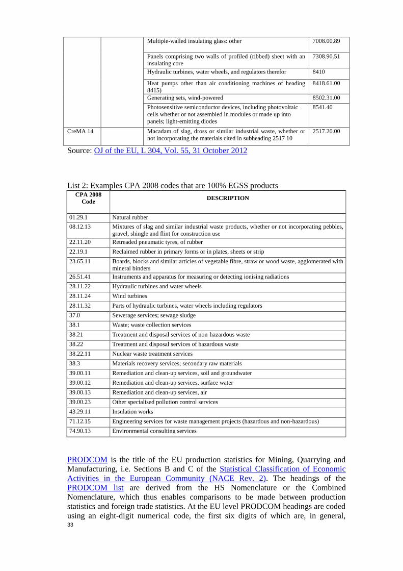
33
Multiple-walled insulating glass: other 7008.00.89
Panels comprising two walls of profiled (ribbed) sheet with an
insulating core
7308.90.51
Hydraulic turbines, water wheels, and regulators therefor 8410
Heat pumps other than air conditioning machines of heading
8415)
8418.61.00
Generating sets, wind-powered 8502.31.00
Photosensitive semiconductor devices, including photovoltaic
cells whether or not assembled in modules or made up into
panels; light-emitting diodes
8541.40
CreMA 14 Macadam of slag, dross or similar industrial waste, whether or
not incorporating the materials cited in subheading 2517 10
2517.20.00
Source: OJ of the EU, L 304, Vol. 55, 31 October 2012
List 2: Examples CPA 2008 codes that are 100% EGSS products CPA 2008
Code DESCRIPTION
01.29.1 Natural rubber
08.12.13 Mixtures of slag and similar industrial waste products, whether or not incorporating pebbles,
gravel, shingle and flint for construction use
22.11.20 Retreaded pneumatic tyres, of rubber
22.19.1 Reclaimed rubber in primary forms or in plates, sheets or strip
23.65.11 Boards, blocks and similar articles of vegetable fibre, straw or wood waste, agglomerated with
mineral binders
26.51.41 Instruments and apparatus for measuring or detecting ionising radiations
28.11.22 Hydraulic turbines and water wheels
28.11.24 Wind turbines
28.11.32 Parts of hydraulic turbines, water wheels including regulators
37.0 Sewerage services; sewage sludge
38.1 Waste; waste collection services
38.21 Treatment and disposal services of non-hazardous waste
38.22 Treatment and disposal services of hazardous waste
38.22.11 Nuclear waste treatment services
38.3 Materials recovery services; secondary raw materials
39.00.11 Remediation and clean-up services, soil and groundwater
39.00.12 Remediation and clean-up services, surface water
39.00.13 Remediation and clean-up services, air
39.00.23 Other specialised pollution control services
43.29.11 Insulation works
71.12.15 Engineering services for waste management projects (hazardous and non-hazardous)
74.90.13 Environmental consulting services
PRODCOM is the title of the EU production statistics for Mining, Quarrying and
Manufacturing, i.e. Sections B and C of the Statistical Classification of Economic
Activities in the European Community (NACE Rev. 2). The headings of the
PRODCOM list are derived from the HS Nomenclature or the Combined
Nomenclature, which thus enables comparisons to be made between production
statistics and foreign trade statistics. At the EU level PRODCOM headings are coded
using an eight-digit numerical code, the first six digits of which are, in general,

34
identical to those of the CPA code. The PRODCOM list is therefore linked to, and
consistent with, the product classification (and thus with the NACE classification).
Going into more detail than CPA, the PRODCOM classification could allow for the
identification of EP and RM output which is not singled out by CPA codes. For
multiple walled insulating units of glass, that is glass used for double windows for
heat saving or noise reduction purposes, are identified by PRODCOM 23.12.13.30,
whereas CPA 23.12.12 also includes glass mirrors. Services are, however, not
covered by PRODCOM. Some more examples of 8-digit PRODCOM goods relevant
for EGSS are shown in List 3 (see below).
List 3: Examples of CPA and PRODCOM Codes relevant for EGSS CPA 2008
Code/
PRODCOM
2008 CodeE
DESCRIPTION
… …
23.12.13 Glass mirrors; multiple walled insulating units of glass
23.12.13.30 Multiple-walled insulating units of glass
… …
23.99.19 Non-metallic mineral products n.e.c.
23.99.19.10 Slag wool, rock wool and similar mineral wools and mixtures thereof, in bulk, sheets or rolls
23.99.19.30 Mixtures and articles of heat/sound-insulating materials n.e.c.
… …
28.25.13 Refrigeration and freezing equipment and heat pumps, except household type equipment
28.25.13.80 Heat pumps other than air conditioning machines
… …
33.2 Installation services of industrial machinery and equipment
33.20.29.10 Installation of engines and turbines (excluding aircraft, vehicle and cycle engines)
… …
The 6-digit-codes of CPA and even the 8-digt codes of PRODCOM may not be
detailed enough to identify environmental goods. Then additional information is
needed to estimate the EGSS shares within a code.
At national level the PRODCOM statistics may be available at a more detailed level
and be used to identify EGSS production. For example, for Germany a list of 254
potential environmental goods has been established using the 9-digit German
PRODCOM version (GP 2009) (Gehrke & Schasse, 2013).
3.5. A map of data integration for EGSS compilation
In the first phase of model development the focus should be on the main areas where
EGSS output and employment can be expected. The estimates should be mainly
based on an integration of data produced regularly by the statistical systems, in
particular supply side statistics (e.g. from the national accounts, SBS and
PRODCOM) as well as demand side data on environmental protection expenditure
and if available on resource management expenditure. Where possible this approach
may be combined with results of EGSS surveys to improve the coverage and quality
of the data. Estimates of EGSS value added and employment can be based on ratios
to output derived from national accounts data broken down by industry.
35
EGSS data cover market activities, non-market activities and ancillary activities and
cover the production of all categories of environmental products. However, in line
with the findings presented earlier the compilation methods proposed do not provide
a cross-classification by environmental product categories. Instead, a pragmatic
categorisation is used as an additional compilation layer to integrate the data. These
categories combine some elements of the market/non-market distinction, the
economic activity by NACE and a distinction between capital and non-capital
products. This categorisation is flexible in accommodating the different sources for
integration. In its basic form it distinguishes the following types of activities:
Market and non-market production of wastewater, waste and water management
services
Market production of EGSS other than wastewater, waste and water management
services: non-capital goods and services
Market production of EGSS: capital goods and services31
Non-market production other than wastewater, waste and water management
services
Ancillary production of EGSS
It has to be stressed that these categories are based on pragmatic considerations for
compilation. The main categories match the source data that should be available for
all countries. Depending on the extra sources available in a country (e.g. specific
EGSS survey among manufacturing industries) additional categories or breakdowns
may be useful.
The integration model combines different statistical sources that may each cover only
subsets of the EGSS, may partly overlap each other (e.g. data from environmental
protection expenditure statistics and investment data from national accounts) or
whose scopes, definitions, classification and valuation principles are different from
the ones needed in the EGSS statistical module. A careful integration approach is
therefore needed to reach a sufficient coverage of the EGSS while avoiding overlaps
and double-counting as far as possible. In Table 1 a map of data used for the
integrative EGSS compilation approach is presented (the approach is described in
detail in chapters 4 to 6 along with the test calculations carried out by Eurostat). This
data map serves to support EGSS compilers solving a puzzle of available sources to
be integrated into an as far as possible consistent picture of the EGSS. An
explanation of the cells of the data map is provided as well.
31
Capital goods and services are generally durable products that through gross fixed capital
formation become (part of) the fixed assets that are used in production for more than one year.
Typical capital products for EP and RM purposes are, for example, gas scrubbers. setting basins
for sewerage, refuses collection vehicles, wind turbines, noise and heat insulating building
materials and their installation.

36
Table 1: EGSS data map
Market and non-
market production of
wastewater, waste
and water
management services
Market production
of EGSS other than
wastewater, waste
and water
management
services: non-capital
goods and services
Market production
of EGSS: capital
goods and services
Non-market
production other
than wastewater,
waste and water
management services
Ancillary production
of EGSS
Protection of
ambient air and
climate
JQ_FP, NA_64,
NA_SUT, LFSJQ_ICE, NA_64, LFS
Wastewater
management
Waste management
Protection of soil,
ground-water, and
surface water
JQ_FP, NA_64,
NA_SUT, LFS, AGRI
(for organic farming)
Noise and vibration
abatement
Protection of
biodiversity and
landscape
Other EP (protection
against radiation, env.
R&D and other env.
protection)
Management of
watersNA_64, NA_SUT, LFS
data not yet
identified, but largely
not applicable
NA_64, NA_SUT,
NA_GFCF, LFS
Production of energy
from renewable
sources
NA_64,NA_SUT,SBS,L
FS,ENSTAT IEA,
FAO/OECD, VNAS (incl. auto-production)
Heat/energy savings
data not yet
identified, but likely
to be small
Material recovery
Other RM
Legend:
= empty cell by definition
= suitable data or methods not yet identified or tested by Eurostat
JQ_ICE: Joint Questionnaire Environmental Expenditure and Revenues: internal current expenditure
JQ_FP: Joint Questionnaire Environmental Expenditure and Revenues: fees and purchases
JQ_INV: Joint Questionnaire Environmental Expenditure and Revenues: investments
NA_64: National accounts aggregates by industries (up to 64 industries) (production and generation of income accounts and employment)
NA_SUT: National accounts supply and use tables (output and intermediate cons. by industries/products, final uses and external trade)
NA_GFCF: Gross capital formation by industry (up to NACE A*64) (by industry and type of asset)
SBS: Structural Business Survey
LFS: Labour Force Survey
ENSTAT: Energy statistics (production qauntities and capacities, prices)
IEA: International Energy Agency: levelised costs and investment costs for electric power stations
FAO/OECD: Biofuel prices
AGRI: Agricultural statistics - land use, farm accountancy
VNAS: Various national sources
RMdata not yet
identified
NA_64, NA_SUT,
NA_GFCF, LFS, VNAS
data not yet
identified, but likely
to be small
NA_64, NA_SUT,
JQ_ICE, LFS
data not yet
identified, but largely
not applicable
EP
JQ_INV, NA_64,
NA_SUT, NA_GFCF,
LFS
JQ_ICE, NA_64, LFS
JQ_ICE, NA_64, LFS
JQ_FP, NA_64, LFS,
NA_SUT
data/methods not yet identified or tested
as far as material recovery is recorded in national accounts under
NACE/CPA E38 it is included in waste management

37
Each white and grey shaded cell of the map should be covered with estimates.
However, for the grey shaded cells no suitable data or methods have yet been
identified and tested by Eurostat; in particular for most resource management areas
suitable EGSS estimation methods need still to be developed in parallel with the on-
going methodological developments for the Resource Management Expenditure
Accounts (ReMEA). Dark shaded cells are empty by definition of the main
categories.
Market and non-market production of wastewater, waste and water management
services
Estimates on output, employment and value added of market and non-market
production of wastewater, waste and water management services can be based on
national accounts data in current prices and national accounts employment data both
broken down by 64 industry groups (NA_64) in combination with information from
the national accounts supply and use tables (NA_SUT) which provide more detailed
information on output cross-classified by 64 product groups and 64 industry groups.
For estimating employment detailed data from the Labour Force Survey may serve as
an additional source.
The most relevant products/industries for this category are CPA/NACE E36 which
covers water collection, treatment and supply and CPA/NACE E37-39 which groups
together sewerage, waste collection, treatment and disposal activities, material
recovery, remediation activities and other waste management services. Additional
data on internal current expenditure on environmental protection (JQ_ICE) can be
used for the separation of E37-39 into wastewater and waste management services if
national accounts data are not detailed enough. Data from the national accounts
supply tables, which present output cross classified by industries and products, can
be used to separate out secondary production that does not fall under wastewater,
waste and water management services and - if applicable - to add secondary output
of these services recorded in other industries. If the national accounts data in the
national statistical institutes (NSIs) are available at a finer industry and product detail
national EGSS compilers should use these finer details, which could in particular
improve the split into wastewater and waste management.
The reason for gathering non-market and market output in one category is that the
split of the total output into non-market and market output is foreseen only as a
secondary compilation step after compiling the total output using national accounts
data. In the test calculations the split was made, but the used national accounts data
available in Eurostat were not detailed enough to produce a satisfactory split. In
order to comply with the amended future Regulation No. 691/2011 it is, however,
necessary to estimate the market output. Therefore some additional investigation in
data and methods sources usable for this split is necessary. Data on general
government expenditure by function (COFOG) may be used as an additional source,
but also more detailed national accounts data available in the NSIs could be useful.
More detail on the estimation of EGSS output under this category is presented in
section 4.1.

38
Market production of EGSS other than wastewater, waste and water management
services: non-capital goods and services
Market production of EGSS non-capital products other than wastewater, waste and
water management services mainly covers the production of services and goods used
for intermediate and final consumption for environmental protection in the area of air
and climate, soil, groundwater and surface water, landscape, biodiversity, noise and
vibration, radiation and environmental protection R&D as well as the production of
energy from renewable sources.
For the EP activities CEPA 1, 3, 5, 6, 7-9 main data sources are the fees and
purchases paid for environmental protection (JQ_FP). The demand side based
approach requires that the data are combined with supply side information. In order
to calculate output cross-classified by industries and to estimate EGSS employment
national accounts data (NA_64) can be used. National accounts supply and use tables
(NA_SUT) provide information on imports and exports by products. This data can be
used to bridge the demand side data to the estimate of output. Agricultural statistics
(AGRI) and farm accountancy data (FADN) in combination with national accounts
data can be used to estimate output from organic farming which is to be recorded
under protection of soil, groundwater and surface water (CEPA 4). For estimating
employment detailed data from the Labour Force Survey may serve as an additional
source.
Information on energy physical production and capacities collected by the energy
statistics (ENSTAT) can be used in combination with national accounts data, price
information and information obtained from energy agencies and various national
sources to obtain output values for the production of electricity from renewable
sources and the production of biofuels and biogas (CReMA 13A).
As far as material recovery is recorded in the national accounts under CPA/NACE
E37-39 it is estimated under the category market and non-market production of
wastewater, waste and water management services as part of CEPA 3 (see above).
The estimates for this category are, however, lower bounds estimates since some
products are unlikely exhaustively covered or at not covered at all.
The demand side data may not fully cover all fees and purchases for EP. For
example, if data on household expenditure are missing in this source some products
are consequently not (exhaustively) covered such as the operation and maintenance
of air pollution control devices for motor vehicles, sewage treatment facilities such as
septic tanks and chemicals to operate them, goods used in connection with waste
management such as bins, bags, composters etc. or low air emission cars or eco-
tourism consumed by private households.
The part of household production of energy that is not delivered to the electricity grid
(e.g. heating energy produced by biomass, geo thermal or solar thermal installations
in private dwellings for own-consumption) is not accounted for in the national
accounts. Extra efforts are therefore needed to include this output in the estimates of
the production of energy from renewable sources.
More detail on the estimation of EGSS output under this category is presented in
section 4.2.

39
Market production of EGSS: capital goods and services
Market production of EGSS capital goods and services covers the production of
services and goods that are used for gross fixed capital formation (investment) for the
protection of the environment and for resource management. These products are
mainly produced by producers of machinery and transport equipment, construction
companies, architects and engineering service providers as well as producers of
computers, electronic products and software.
In the absence of specific EGSS surveys this category can be estimated using
demand side data, in particular data on investments specifically for environmental
protection (JQ_INV). Also data on gross fixed capital formation from the national
accounts provide information which may be used to estimate the supply of EGSS
capital goods and services, in particular investments by those industries that are
characteristic or play an important role for environmental protection and resource
management.
Information on investments by type of asset (NA_GFCF) can be useful in order to
map the data broken down by investing industries to the industries that produce the
capital products.
National accounts supply and use tables provide information on imports and exports
by CPA product which can help to bridge the demand side data to the estimate of
output.
Information on the change in energy producing capacities collected by energy
statistics (ENSTAT) in combination with information obtained from energy agencies
and various national sources are useful to derive estimates on investments in the area
of renewable energy and heat/energy savings.
PRODCOM statistics may also be used if the EGSS shares of the PRODCOM codes
are known. For some goods the EGSS shares may be assumed as close to 100% so
that PRODCOM statistics may serve directly as a complementary source (e.g. for
wind powered generating sets and multiple-walled insulating units of glass).
More detail on the estimation of EGSS output under this category is presented in
section 4.3.
Non-market production other than wastewater, waste and water management
services
Non-market (government) production other than wastewater, waste and water
management services can also be based on demand side data, in particular data on
internal current expenditure on environmental protection (JQ_ICE) by the public
sector. Conceptually, internal current expenditure provides a lower bound estimate of
government output (which is to be measured using the cost approach). This lower
bound estimate may be upgraded using factors derived from national accounts data to
represent the cost share equivalent to the consumption of fixed capital.
More detail on the estimation of EGSS output under this category is presented in
section 4.4.

40
Ancillary production of EGSS
Ancillary production is not measured within the national accounts framework. A
source available to derive estimates of ancillary EGSS output is data on the internal
current expenditure for environmental protection (JQ_ICE). National accounts data
broken down by activity may, however, be used to provide a more detailed split of
ancillary output by industry and to derive indicators of the employment linked with
the production of ancillary output.
More detail on the estimation of EGSS output under this category is presented in
section 4.5.
41
4. TEST CALCULATION FOR EGSS OUTPUT
The test calculations are described in some detail to provide methodological support
to national EGSS compilers. The test calculations for EGSS output as well as those
for EGSS employment (chapter 5) and EGSS gross value added (chapter 6) have
been compiled by Eurostat through an integration of data mainly available in the
database on Eurostat’s website32
. This does not mean that it is proposed to use data
downloaded from this database only; the national statistical institutes should use data
from their own databases, which may provide additional and more detailed
information usable for EGSS compilation. However, if EGSS data can be compiled
with data in Eurostat’s publicly accessible database and other publicly and freely
accessible sources, Member States should at least be able to achieve the same
minimum standard in EGSS compilation as proposed by this guide.
The structure of this chapter follows the structure of the pragmatic categories of
activities of the data map presented in section 3.4. The chapter describes in some
detail the data sources and methods as well as results obtained. At the end of the
sections proposals for improvements are also made.
The scope of the test calculations is as follows:
They cover annual data for the years 2000-2012 (of which only the period 2007-
2011 is shown in this guide). The variables compiled are output, exports, gross
value added and employment. Whereas the reporting requirements of Regulation
No. 691 cover market activities only, the test calculations also cover non-market
and ancillary activities.
The breakdown by CEPA classes (EP activities) corresponds to the reporting
requirements of Regulation No. 691, i.e. CEPA 1, 2, 3, 4, 5, 6 and one aggregate
covering CEPA 7, 8, 9.
In the test calculation the reporting by CReMA classes (RM activities) does not
fully comply with the reporting requirements of Regulation No. 691. The test
calculations cover CReMA 10 (management of water) as well as CReMA 13A
(production of energy from renewable sources) and 13B (heat/energy savings and
management). If material recovery to be recorded under CReMA 11B
(management of the intake of forest resources), CReMA 13C (minimisation of the
intake of fossil resources as raw material) or CReMA 14 (management of
materials) are included in the sources used to estimate waste management
activities they will be reported in the test calculations under CEPA 3. Estimation
approaches for the other CReMA classes not yet covered by the test calculations
will be developed in parallel with the developments for the Resource Management
Expenditure Accounts (ReMEA).
The reporting by CEPA/CReMA is cross classified by those 39 NACE industry
categories that have also been distinguished in the 2014 voluntary data
collection33
. However, in the test calculations it was not possible to identify EGSS
activities in all of these 39 NACE categories either due to lack of data or because
32
To some extent also national and international sources have been used. For an overview of the
sources used see also annex F.
33 Regulation No. 691/2011 requires a less detailed breakdown by 21 industries (NACE A*21).
However, for the voluntary data transmission it is envisaged to maintain the more detailed
breakdown. For details on the various aggregation levels see also annex E.

42
the sources used (e.g. the supply tables) did not signify any relevant activities in
the categories.
4.1. Market and non-market production of wastewater, waste and water
management services
This category can be identified from national accounts (NA) data for NACE section
E (water supply; sewerage, waste management and remediation activities). In this
specific NACE section producers whose principal activity is the production of
environmental services are found.
4.1.1. Supply side approach for wastewater management and waste
management services
Output of wastewater and waste management services can be compiled from NA
data broken down by industries and from supply tables. The core matrix of a supply
table provides information on the output of the economy broken down by industries
(table columns classified by NACE) and products (table rows classified by CPA),
whereby the classifications of industries and products are fully aligned to each
other34
.
The test calculations start from Eurostat’s collections ‘National Accounts aggregates
by industry (up to NACE A*64) (nama_10_a64)’35
and ‘Supply table - current prices
(NACE Rev. 2) (naio_cp15_r2)’. The first collection provides output data by 64
industries. The supply tables provide output data cross-classified by 64 industries and
64 products from which shares of the relevant CPA category E37-39 in the total
output of each of the 64 industries can be derived.
The national accounts data by 64 industries are mapped to the 39 NACE categories
of the EGSS module (see annex E). Then, in multiplying the output values from the
mapped data with CPA E37-39 output shares derived from the supply tables CPA
E37-39 output for each of the 39 NACE industries of the EGSS module can be
calculated36
. This is the basis for deriving the EGSS output variables as it is shown in
the next paragraphs.
Output of wastewater management (CEPA 2) and waste management (CEPA 3)
services in these collections are covered by the product group CPA E37-39, so that
sums of CEPA 2 and CEPA 3 output for each industry can be calculated:
34
See also Statistics Explained Article: Building the System of National Accounts - supply and use
tables
35 For countries, for which the new ESA 2010 data were not available the collection ‘annual
National Accounts by 64 branches at current prices (nama_nace64_c)’ has been used.
36 For the test calculations supply tables are not available for all years in all countries. If supply
table data are missing for certain years some gap-filling is applied based on the observation that
the output shares are rather stable over time. In such cases the time trends for CPA E37-39 output
by the 39 industries follow the changes in the total output by industries.

43
EGSS_P1_ServCEPA 2,nace + EGSS_P1_ServCEPA 3,nace = NA_P1CPA E37-39, nace
NA_P1CPA E37-39, nace: Output of product group CPA E37-39 by industries (NA)
EGSS_P1_ServCEPA 2,nace: Output of wastewater management services by industries (EGSS)
EGSS_P1_ServCEPA 3,nace: Output of waste management services by industries (EGSS)
The division within CPA E37-39 relevant for CEPA 2 is CPA E37 (sewerage)
whereas CPA E38 (waste collection, treatment and disposal activities; material
recovery) and CPA E39 (remediation activities and other waste management
services) are relevant for CEPA 3. The split of CPA E37-39 into wastewater and
waste management is based on a share approach. The shares (sCEPA 2 and sCEPA 3) are
estimated using data on internal current expenditure on wastewater management and
waste management by private and public specialised producers of EP services from
the Joint Eurostat/OECD Questionnaire on Environmental Expenditure and
Revenues (JQ-EPER)37
.
Applying these shares to CPA E37-39 gives an estimate of the production of
wastewater management and waste management services in each relevant industry:
EGSS_P1_ServCEPA 2,nace = NA_P1CPAE37-39,nace * sCEPA 2
EGSS_P1_ServCEPA 3,nace = NA_P1CPAE37-39,nace * sCEPA 3
For sake of simplicity, it is assumed that all wastewater management output of the
group NACE E37-39 is produced by NACE E37 and that all waste management
output of the group NACE E37-39 is produced by NACE E38 and NACE E39. Such
simplification can be avoided if national accounts data are available in a more
detailed industry breakdown for the group NACE E37-39 or if additional data can be
used for the split. In additional calculations such a split has been tested using the
same factors as already used for the split of output into CEPA 2 and CEPA 338
.
However, the result of this test seemed not be plausible, since output of wastewater
management services in industry NACE E37 (sewerage) would be lower than in
industry NACE E38 (waste collection, treatment and disposal activities). Unless this
result would be strongly confirmed by additional information it was felt that the
simplified assumption is less problematic than the splitting approach. In this context
it is to be noted that the reporting requirements of Regulation No. 691 are less
detailed: within the required A*21 NACE grouping the activities in question would
be grouped within NACE E36-39.
37
For example, for Germany the shares vary slightly over the years around the approximate values
of sCEPA 2≈0.4 and sCEPA 3≈0.6. For more details on the used source see section 4.5 on ancillary
output.
38 In order to split NACE E37-39 into E37 and E38-39 the shares sCEPA 2 and sCEPA 3 were used in a
test calculation for Germany. For the further split of NACE E38-39 into NACE E38 and NACE
E39 a ratio of 9:1 was assumed. This approach ensures consistency of the split data with the
overall totals for NACE/CPA E37-39.

44
Table 2a: Test calculation: Market and non-market output of wastewater
management services, Germany (million EUR)
2007 2008 2009 2010 2011
Total NACE
15333 15333 15333 15333 15333
D 342 369 447 454 449
E36 892 914 747 649 693
E37 14099 14016 13841 14004 15742
Table 3a: Test calculation: Market and non-market output of waste management
services, Germany (million EUR)
2007 2008 2009 2010 2011
Total NACE
24946 25974 24216 26617 29748
D 557 627 719 799 791
E36 1451 1552 1203 1144 1221
E38 20645 21415 20065 22206 24963
E39 2294 2379 2229 2467 2774
The approach described above identifies wastewater and waste management services
are identified as principal output of NACE E37-39 and secondary output of other
industries. For Germany, wastewater management services output is identified as
principal output of NACE E37 and as secondary output in NACE D (electricity, gas
steam, and air conditioning supply) and NACE E36 (water collection, treatment and
supply). Waste management services output is identifies as principal output of
NACE E38 and NACE 39 and as secondary output in NACE D (electricity, gas
steam, and air conditioning supply) and NACE E36 (water collection, treatment and
supply). The breakdown of wastewater and waste management output by industry as
shown in the table above is specific for Germany and not indicative for other
countries. Using the same compilation method for other countries may identify
wastewater management services also in other industries such as mining and
quarrying, in manufacturing industries, construction, wholesale and retail trade and
for public administration (depending on the information in the supply tables).
When supply tables are not available an alternative, simpler approach is to use total
output figures of NACE E37-39 (not broken down by CPA codes), which are
available in the collection ‘National Accounts aggregates by industry (up to NACE
A*64) (nama_10_a64)’:
EGSS_P1_ServCEPA 2, NACE E37 = NA_P1NACE E37-39 * sCEPA 2
EGSS_P1_ServCEPA 3, NACE E38 = NA_P1 NACE E37-39 * sCEPA 3
NA_P1NACE E37-39: Total output of industry group NACE E37-39 (NA)

45
This simplified estimation of wastewater and waste management may, however,
include some secondary output of NACE E37-39 that is not related to wastewater
and waste management and does not include any secondary wastewater and waste
management services produced by other industries.
Regulation (EU) No. 691 requires reporting on market output. Therefore output of
wastewater and waste management services needs to be split into non-market and
market output using share estimates (sharenon-market,nace):
EGSS_P11_ServCEPA 2,nace,non-market = EGSS_P1_ServCEPA 2,nace, *(1-sharenon-market,nace)
EGSS_P13_ServCEPA 2,nace,non-market = EGSS_P1_ServCEPA 2,nace, * sharenon-market,nace
EGSS_P11_ServCEPA 3,nace,non-market = EGSS_P1_ServCEPA 3,nace, *(1-sharenon-market,nace)
EGSS_P13_ServCEPA 3,nace,non-market = EGSS_P1_ServCEPA 3,nace, * sharenon-market,nace
EGSS_P11_ServCEPA 2,nace: Market output of wastewater management services by industries (EGSS)
EGSS_P11_ServCEPA 3,nace: Non-market output of waste management services by industries (EGSS)
EGSS_P13_ServCEPA 2,nace: Non-market output of wastewater management services by industries
(EGSS)
EGSS_P13_ServCEPA 3,nace: Non-arket output of waste management services by industries (EGSS)
For the test calculations the main source to calculate this split are the national
accounts supply tables, from which shares of non-market output in the total output of
the single industries can be estimated:
sharenon-market,nace = NA_P1P13,nace / NA_P1CPA_Total,nace
It is, however, to be noted that the supply tables available in Eurostat do not provide
information on this split cross-classified by products and industries. Data available in
the national statistical offices may help to overcome these limitations and allow
further refinement of the approach.
A further limitation when estimating non-market shares is missing data: in the test
calculations it was observed that data for non-market output by industries were not
available in all countries’ supply tables. As an additional source to separate non-
market from market output data on government current internal expenditure on
wastewater and waste management from the Joint Eurostat/OECD Questionnaire on
Environmental Protection Expenditure and Revenues (JQ-EPER) is therefore used.
The approach is to calculate the difference between internal current expenditure of
government and non-market output of wastewater and waste management services in
NACE O (as calculated by the approach described above), to allocate this difference
to non-market output in NACE E37-39, and then to derive an alternative estimate for
the non-market output share of NACE E37-39. If the alternative share is bigger than
the non-market output share for NACE E37-39 obtained by using supply table
information, the alternative share is used in the calculations. In situations where

46
supply tables do not include data on non-market output and do not allocate some part
of CPA E37-39 to NACE O, the non-market share of wastewater and waste
management is thus based on the information from the JQ-EPER.
Furthermore, when using this approach it is also recommended to cross-check the
results obtained with data available in the COFOG statistics.
Table 2b: Test calculation: Split between market and non-market output of
wastewater management services, France (million EUR)
2007 2008 2009 2010 2011
Non-market
2632 2825 2911 3119 3145
Market 9604 10073 8777 10366 10785
Table 3b: Test calculation: Split between market and non-market output of waste
management services, Spain (million EUR)
2007 2008 2009 2010 2011
Non-market
2742 2888 5112 5361 5363
Market 9713 10202 6892 7200 7192
Future improvements
At a later stage of the development of the compilation framework the estimates may
be further refined and completed:
The simplifying assumption on the allocation of wastewater and waste management
services to the producing NACE divisions within NACE group NACE E37-39
should be reviewed. Additional data may be found for this purpose, for example, it
could be explored whether an improved split of these services among the divisions
could be made by using SBS data, company data or simply by more detailed national
accounts data available in the national statistical institutes.
The recovery of sorted materials which is recorded under NACE E38 may include
activities that are resource management activities such as minimisation of the intake
of forest resources, minimisation of the intake of fossil resources as raw material for
use other than energy production, management of minerals. Allocating material
recovery to resource management requires separating the activities by materials. A
split of the NACE-based data may be possible using additional data (e.g. physical
data on the quantities of materials recovered) from extra sources (e.g. information
from business associations or from the Eurostat Environmental Data Centre on
Waste). However, making this split is likely to be time consuming so that in the
current phase of the model development this split is not made.
Waste management should also include street cleaning. Street cleaning is, part of
cleaning NACE N81.29 (other cleaning activities). It may therefore be identified
from detailed NA or SBS data in combination with additional information on the
share of street cleaning within the class. Alternatively, it may be explored whether
47
street cleaning can be identified from other sources (e.g. from government
expenditure data classified under COFOG group 05.1 waste management).
Since production recorded under NACE E39 may also include activities related to
the protection and remediation of soil, groundwater and surface water that fall under
CEPA 4, it should be considered to separate out these activities as part of the future
development of the approach.
4.1.2. Supply side approach for water management services
Management of water is a resource management activity and comprises activities
aimed at the minimisation of inland waters intake through in-process modification as
well the reduction of water losses and leaks or reduction of the intake by substituting
the resources with alternative resources, the installation and construction of facilities
for water reuses and savings, shower heads and taps. The 2009 EGSS handbook (p.
61) recommends not including the distribution, collection and potabilisation of water.
On the basis of data available in Eurostat’s database it is not possible to derive an
estimate from the demand side. Data on government expenditure by function
(COFOG) have no separate group for management of water and the satellite accounts
for resource management expenditure (ReMEA) are still under development.
Principal producers of water management services can be found under NACE E36
(water collection, treatment and supply) and the characteristic product under the
corresponding CPA E36 category. With the recommendations of the 2009 EGSS
handbook being followed only a part of NACE/CPA E36 is included under CReMA
10.
Based on the data available in Eurostat it seems to be difficult to narrow the scope of
water management from NACE/CPA 36 to the definition of resource management
which would have to exclude the distribution, collection and potabilisation of water.
Estimations for France (Greffet, Mauroux, Ralle, & Randriambololona, 2012) show
that employment for production and distribution of water is five times higher than for
the resource management of water. In the cited above publication resource
management of water is considered as being part of the “eco-activities” whereas the
production and distribution of water is included in the broader definition of “green
economy activities”. Future developments of the resource management expenditure
accounts (ReMEA) may lead to an improved data availability that may help to
overcome data gaps for the estimation of water resource management activities. An
important area to focus on in the future is water management. (Eurostat, 2013c).
Output of water management services can be estimated analogously to the approach
used for wastewater and waste management services. The test calculations start from
Eurostat’s collections ‘National Accounts aggregates by industry (up to NACE
A*64) (nama_10_a64)’39
and ‘Supply table - current prices (NACE Rev. 2)
(naio_cp15_r2)’. The first collection provides output data by 64 industries. From the
supply tables shares of the relevant CPA category E36 in the total output of each of
the 64 industries can be derived. Before using the data of ‘nama_nace64_c’ its 64
industries must be mapped to the 39 NACE categories of the EGSS module. Then, in
multiplying the output values from the mapped data with the CPA E36 output shares
39
For countries, for which the new ESA 2010 data were not available collection ‘annual National
Accounts by 64 branches at current prices (nama_nace64_c)’ is used.

48
CPA E36 output for each of the 39 NACE industries of the EGSS module can be
calculated. A factor f may take into that the water management (CReMA 10) is only
a fraction of CPA 36 output (see above). This is the basis for deriving the EGSS
output variables as it is shown in the next paragraphs.
The output of CPA E36 by the 39 industries is then allocated to CReMA 10:
EGSS_P1_ServCReMA 10,nace = NA_P1CPA E36,nace * f
NA_P1CPA E36, nace: Output of product CPA E36 by industries (NA)
EGSS_P1_ServicesCReMA 10,nace : Output of water management services by industries (EGSS)
Analogously to the simplification made for wastewater and waste management, it is
assumed that all CPA36 output of the group NACE E37-39 is allocated to NACE
E37. In this context it is to be noted that the reporting requirements of Regulation
No. 691 are less detailed: within the A*21 NACE grouping management of water by
NACE E36, E37, E38 and E39 would be grouped to NACE E36-39.
Table 4a: Test calculation: Market and non-market output of water management
services, France (million EUR)
2007 2008 2009 2010 2011
Total NACE
1849 1909 1984 1971 1911
E36 1845 1905 1979 1965 1906
O 4 4 5 4 5
P 0 0 1 1 1
Note that by applying the approach described above water management output is
identified as principal output of NACE E36 and secondary output of other industries.
For France, water management output is identified as principal output of NACE E36
and to some minor extent as secondary output in other industries. This breakdown of
water management output by industry is specific for France (based on the supply
tables); it is not indicative for other Member States. For example, in using the same
approach for the United Kingdom no water management services outside NACE E36
is identified.
In the case that supply tables are not available an alternative, simpler approach would
be to use the total output of NACE E36 (available in collection ‘(nama_10_a64)’):
EGSS_P1_ServCReMA 10,NACE E36 = NA_P1NACE E36 * f
NA_P1NACE E36: Total output of industry NACE E36 (NA)
This alternative estimate of water management services may include some secondary
output of the NACE E36 that is not related to water management (e.g. sewerage) and
does not include any secondary water management produced by other industries. It is
therefore worth mentioning that using this alternative estimate for water management

49
services can lead to double counting of secondary sewerage services by NACE E36
if for wastewater management services the more detailed approach using supply table
information (see section 4.1.1) is used; in this case secondary output of sewerage
may be reported twice as wastewater management and management of water.
Therefore it is recommended to use either the more detailed approach (using supply
table information) for both, wastewater management and management of water, or
the simplified approach for both, wastewater management and management of water.
Regulation (EU) No. 691/2011 requires reporting on market output. Therefore the
output of water management services needs to be split into non-market and market
output. Basically, in the test calculations, to make this split, an approach analogous to
the one already described for wastewater and waste management services (see
section 4.1.1) is used. However, since resource management expenditure statistics
are still less developed than environmental protection expenditure statistics, the
calculation approach for wastewater management uses information available in the
supply tables only. When there is no information in this source on the non-market
output it is assumed that all water management services are market production. Data
available in the national statistical offices may help to overcome these limitations of
the approach..
Table 4b: Test calculation: Split between market and non-market output of water
management services, Spain (million EUR)
2007 2008 2009 2010 2011
Non-market
43 44 385 402 404
Market 2150 2242 2015 2101 2115
Future improvements
At a later stage of the development of the compilation framework the estimates may
be further refined and completed.
Some activities of management of water may also be found under CPA/NACE
categories other than those belonging to NACE section E. For example, installation
of water efficient irrigation systems should be recorded under NACE A01.61
(support activities for crop production) and R&D and education services related to
management of water under NACE M72 and NACE P85, respectively. The
identification of water managements services under these and other NACE/CPA
categories may be possible with more detailed breakdowns than those available for
the test calculations. But even with a CPA breakdown by 6-digits they normally
cannot be identified so that even more detailed information (e.g. based on specific
surveys among providers of architectural and engineering services, R&D and
education services) would be needed. It would be sufficient to observe such more
detailed data in greater intervals (e.g. every 5 years) in order to interpolate the
interim years by using constant shares.
With resource management expenditure accounts being further developed and future
pilot data collections in this area, it would be possible to further improve estimation
of water management services. Possible areas that could be improved using more
detailed information are the exclusion of water services not related to resource
management and the split into market and non-market output.

50
4.2. Market production of EGSS other than wastewater, waste and water
management services: non-capital goods and services
In this practical guide the use of demand side data on environmental protection
expenditure collected from the JQ-EPER is proposed for the following
environmental protection activities: protection of ambient air and climate (CEPA 1),
protection and remediation of soil, groundwater and surface water (CEPA 4), noise
and vibration abatement (CEPA 5), protection of biodiversity and landscapes (CEPA
6) and other environmental protection activities (CEPA 7+8+9). Details on the
approach are shown in section 4.2.1.
In accordance with the recommended approach of the 2009 EGSS handbook output
of organic farming is considered to lie within the scope of EGSS and contributes to
CEPA 4. Supply side data can be used to estimate output of organic farming. Details
on the approach are shown in section 4.2.2.
Supply side data is also used to estimate the production of electricity from renewable
sources as part of CReMA 13A (for details see section 4.2.3). Estimates for other
forms of renewable energy (such as biofuels and biogas) are based on price times
quantity approaches (for details see section 4.2.4 and 4.2.5). Following the
recommendation of the Eurostat Task Force (TF) on the resource management
expenditure account (ReMEA) (Eurostat, 2013d) this practical guide excludes the
production of biomass (wood etc.) that is converted into other forms of energy which
are then sold from the scope of CReMA 13A. The accounting for the biomass used
for that part that is not converted into marketed energy products (e.g. wood or wood
pellets used by households for own consumption) is not covered by this practical
guide and is a potential area for future research (see also annex C, revision item 7c).
Summarised results of the test calculations for this category are shown in section
4.2.6.
The methods proposed in this section of the practical guide may be combined with
other approaches based on surveys, SBS data and lists of PRODCOM codes.
4.2.1. Demand side approach for the production of environmental
protection services
Some production of EGSS non-capital services can be identified using demand side
data on fees and purchases from the JQ-EPER dataset. Fees/purchases (JQ_FPcepa)
should include all purchases of environmental protection services, both from public
and private producers. These payments are clearly linked with an environmental
protection (EP) activity outside the enterprise and should exclude e.g. fines and
penalties. Payments of taxes directly used for financing environmental protection
expenditure and payments of general environmental or green taxes (such as energy
taxes) are excluded.
For the compilation of EGSS data the expenditure must be mapped to the producing
NACE industries. In this phase of model development it is assumed, for reasons of
simplicity, that output of non-capital EGSS products for EP other than wastewater
and waste management services is found in only a few industries. More specifically,
fees/purchases other than for wastewater, waste and water management services are

51
assumed to be for services produced in NACE section M (professional, scientific and
technical activities):
EGSS_P1_Servcepa,NACE M = JQ_FPcepa; cepa = CEPA 1, CEPA, 4, CEPA 5, CEPA 6, CEPA 7-9
EGSS_P1_Servcepa,NACE M: Output of EP services of NACE section M by CEPA classes (EGSS)
JQ_FPcepa: Fees/purchases for EP by CEPA classes (JQ-EPER)
The split into NACE divisions (NACE M69_70, M71 etc.) is made using relative
shares of each division (s) in total NACE M output from national accounts, e.g. with
NACE group M69-70 used as an example:
EGSS_P1_Servcepa, NACE M69_70 = JQ_FPcepa * s NACE M69_70, NACE M
where s NACE M69_70, NACE M = NA_P1NACE M69_70 / NA_P1NACE M
EGSS_P1_Servcepa,NACE M69_70: Output of EP services of NACE group M69_70 by CEPA classes
(EGSS)
NA_P1NACE M69_70: Total output of NACE group M69_70 (NA)
NA_P1NACE M: Total output of NACE section M (NA)
When mapping expenditure to EGSS output we must consider that expenditure
excludes exports but includes imports and that expenditure is valued at purchase
prices whereas output should be valued at basic prices. Hence some corrections need
to be made. The problem of export-import adjustment may be tackled by an analysis
of detailed external trade data. However, in this practical guide a less time
consuming approach is proposed: to derive corrections factors using data from
national accounts supply and use tables.
The use tables of the national accounts provide data on the use of products for
intermediate consumption (IC), final consumption (FC), gross capital formation
(GCF) and exports (EX), whereas the supply table columns provide information on
imports (IM), trade and transport margins (TM) and taxes less subsidies on products
(TS) broken down by CPA product. To adjust expenditure based data correction
factors (f) can be compiled:
f = 1+(EX-IM-TM-TS)/(IC+FC+GFC)
These factors form a bridge between the demand side and the supply side and capture
also valuation differences.
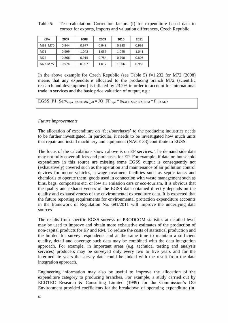
52
Table 5: Test calculation: Correction factors (f) for expenditure based data to
correct for exports, imports and valuation differences, Czech Republic
CPA 2007 2008 2009 2010 2011
M69_M70 0.944 0.977 0.948 0.988 0.995
M71 0.999 1.048 1.039 1.045 1.041
M72 0.866 0.915 0.754 0.790 0.806
M73-M75 0.974 0.997 1.017 1.006 0.982
In the above example for Czech Republic (see Table 5) f=1.232 for M72 (2008)
means that any expenditure allocated to the producing branch M72 (scientific
research and development) is inflated by 23.2% in order to account for international
trade in services and the basic price valuation of output, e.g.:
EGSS_P1_Servcepa, NACE M69_70 = JQ_FPcepa * sNACE M72, NACE M * fCPA M72
Future improvements
The allocation of expenditure on ‘fees/purchases’ to the producing industries needs
to be further investigated. In particular, it needs to be investigated how much units
that repair and install machinery and equipment (NACE 33) contribute to EGSS.
The focus of the calculations shown above is on EP services. The demand side data
may not fully cover all fees and purchases for EP. For example, if data on household
expenditure in this source are missing some EGSS output is consequently not
(exhaustively) covered such as the operation and maintenance of air pollution control
devices for motor vehicles, sewage treatment facilities such as septic tanks and
chemicals to operate them, goods used in connection with waste management such as
bins, bags, composters etc. or low air emission cars or eco-tourism. It is obvious that
the quality and exhaustiveness of the EGSS data obtained directly depends on the
quality and exhaustiveness of the environmental expenditure data. It is expected that
the future reporting requirements for environmental protection expenditure accounts
in the framework of Regulation No. 691/2011 will improve the underlying data
sources.
The results from specific EGSS surveys or PRODCOM statistics at detailed level
may be used to improve and obtain more exhaustive estimates of the production of
non-capital products for EP and RM. To reduce the costs of statistical production and
the burden for survey respondents and at the same time to maintain a sufficient
quality, detail and coverage such data may be combined with the data integration
approach. For example, in important areas (e.g. technical testing and analysis
services) producers may be surveyed only every two to five years and for the
intermediate years the survey data could be linked with the result from the data
integration approach.
Engineering information may also be useful to improve the allocation of the
expenditure category to producing branches. For example, a study carried out by
ECOTEC Research & Consulting Limited (1999) for the Commission’s DG
Environment provided coefficients for the breakdown of operating expenditure (in-

53
house expenditure and purchases) for environmental activities by compensation of
employees, energy, intermediate goods, capital goods and private services and public
services (see table below). However, before such coefficients can be used it must be
examined whether they are still applicable for the country under study or whether
they need to be updated using country specific engineering information.
Table 6: Engineering information on the breakdown of operating expenditure in
environmental protection activities
Env. activity Compensation of
employees Energy Intermediate
Goods Capital Goods
Private Services
Public Services
Air pollution control 15% 35% 45% 5%
Wastewater treatment 40% 20% 20% 10% 10%
Waste management 60% 10% 10% 10% 10%
Remediation and Clean up of Contaminated Land and Water
20% 30% 50%
Noise and Vibration Control
65% 5% 30%
Source: ECOTEC Research & Consulting Limited (1999), annex of the ECOTEC study
The correction factors (f) for international trade and valuation differences may need
further investigation. In particular, factors based on A*64 NACE/CPA aggregates
may not be sufficiently representative for EGSS producers within those industries. A
more detailed analysis of external trade in EGSS products based on external trade
statistics may be necessary.
4.2.2. Supply side approach for organic farming products
A very simple estimate of the output from organic farming may be compiled by
multiplying the share of land use for organic farming in total utilised agricultural area
with national accounts (NA) data on agricultural output.
EGSS_P1_FarmProdCEPA 4, NACE A = NA_P1NACE A01 * Landorg/Landtotal:
EGSS_P1_FarmProdCEPA 4, NACE A: Output of organic farm products by NACE section A (EGSS)
NA_P1NACE A01: Total output of crop and animal production, hunting and related service activities
(NACE A01) (NA)
Landorg: Land use for organic farming
Landtotal: Total utilised agricultural area
The data on land use are available in Eurostat’s agricultural statistics, namely in the
collections ‘certified organic crop area (food_in_porg1)’ and ‘Land use - 1 000 ha -
annual data (apro_cpp_luse)’.
If available more detailed accounting information on organic farming can be
integrated into the approach. For example, instead of assuming that the output value
of farming is distributed between organic and conventional farming simply according
to land shares, specific bookkeeping information on organic and conventional
agriculture may be used to reflect different productivities and prices for the two types

54
of farming. For the test calculations for Germany it was assumed that the ratio
between per-ha turnover of organic farming and conventional is approximately
r≈0.740
.
Using this information and combining it with national accounts data on agricultural
output, total utilised agricultural area and land use for organic farming, allows
deriving indicators of output per ha for conventional and organic farming:
Prodconv/ha = NA_P1NACE A01 / [(Landtotal - Landorg)+ Landorg * r]
Prodorg/ha = Prodconv/ha * r
Prodconv/ha: Output per hectare in conventional farming
Prodorg/ha: Output per hectare in organic farming
r: ratio ‘per-ha turnover of organic farming / per-ha turnover of conventional farming’
Table 7: Test calculation: Output per ha in organic and conventional farming,
Germany (EUR/ha)
2007 2008 2009 2010 2011
organic farming
1755 1921 1733 1941 2055
conventional farming
2507 2752 2386 2524 2797
Output of organic farm products is then calculated by multiplying output per ha in
organic farming by the size of the organic farmland area. Output of organic farming
is allocated to NACE section A (agriculture, forestry and fishing) and to CEPA 4
(protection and remediation of soil, groundwater and surface water).
EGSS_P1_FarmProductsCEPA 4, NACE A = Prodorg/ha * Landorg
40
For the test calculation for Germany the results of a special examination of bookkeeping data
from the German Farm Accountancy Data Network carried out by a German research agency
(Thünen-Institut, 2013) were further analysed to derive ratios of turnover per ha between organic
and conventional farming. The data suggest that turnover per ha in organic farming is higher than
in conventional farming for dairy and fodder production, whereas it is lower for other farm types.
From the bookkeeping data it may be derived that turnover per ha in the period 2008/09 to
2011/12 was only up to 10% lower in organic farming than in conventional farming. However,
the comparison is driven by the underlying purpose “to deduce what profit the organic farms
would make if they were managed conventionally” (Offermann, Sanders, & Nieberg). A press
release by the Federal Ministry Food, Agriculture and Consumer Protection (Bundesministerium
für Ernährung, Landwirtschaft und Verbraucherschutz, 2012b) informs that in 2010 average
turnover per ha of organic farming was 40% lower than for conventional farms. For the test
calculations it was assumed that the ratio between per-ha turnover of organic farming and
conventional is approximately r≈0.7.

55
Future improvements
An alternative source for total output of farming than national accounts NACE A01
is the Economic Accounts for Agriculture (EAA) (Eurostat, 2000). Some definitional
differences between national accounts data and the EAA that may be relevant for
EGSS data compilation should be considered:
Output in EAA includes intra-unit consumption of fodder, whereas intra-unit
deliveries are not included in output by the national accounts.
The EAA excludes the separable non-agricultural secondary output of holdings,
whereas the national accounts division A01 includes all support activities to
agriculture and post-harvest crop activities (NACE A01.6) such as for example,
the provision of agricultural machinery with operators and crew, agricultural
activities on a fee basis (e.g. activities related to artificial insemination), the
preparation of crops for primary markets as well as seed processing for
propagation.
The EAA includes parts of the processing of agricultural goods (mainly grapes to
wine and olives to olive oil) if this is carried out by groups of producers (e.g. co-
operatives), whereas in national accounts this activity is to be recorded under
NACE C10 (manufacture of food products) and NACE C11 (manufacture of
beverages).
Whether the national accounts scope of NACE A01 or the EAA scope is more
relevant for deriving EGSS data on organic farming cannot be decided a-priori and
depends on the relative importance of the various elements of scope differences. If
EAA data are used, must intra-unit consumption of fodder be excluded from the
EGSS estimate of organic farming as well as output from non-agricultural secondary
output of holdings and any processing of primary agricultural products to food and
beverages? Should, on the other hand, support activities to agriculture and post-
harvest crop activities be included in EGSS if they serve a primary EP or RM
purpose? The EAA as a satellite account should be detailed enough to provide a good
approximation to what is needed to estimate output from organic farming.
The approach sketched above and applied in the test calculation for Germany is an
implicit ‘quantities times prices’ approach. An explicit quantity times price approach
would multiply quantities of organic farm products with the respective prices of the
organic farm products. Data on the quantities of organic farm production are
available in Eurostat’s collections Certified organic crop production and yields from
fully converted areas (food_in_porg2)’ and ‘Certified production of organic animal
products (food_pd_dmorg)’. The main challenge with this explicit approach would
be to collect representative prices for organic farm products. The data in Eurostat’s
collections ‘Selling prices of crop products (absolute prices) - annual price (from
2000 onwards) (apri_ap_crpouta)’ and ‘Selling prices of animal products (absolute
prices) - annual price (from 2000 onwards) (apri_ap_anouta)’ do not distinguish
between conventional and organic farm products.
4.2.3. Supply side data approach for electricity produced from
renewable sources
The production of electricity production from renewable sources is part of CReMA
13 A (production of energy from renewable sources). The estimation approach for

56
electricity production from renewable sources can be organised top-down starting
with national accounts data broken down by industries and accounts supply tables
and then stepwise integrating information on the physical production of electricity by
the various available technologies and data on maintenance and operational costs
(compare also with Voram & van Rossum, 2013).
The core matrix of a supply table provides information on the output of the economy
broken down by industry (table columns classified by NACE) and products (table
rows classified by CPA). Firstly, the NACE/CPA codes that cover production of
electricity from renewable sources have to be identified. Then the share of electricity
production from renewable sources needs to be estimated using additional
information from other sources such as energy statistics. In what follows we show
details of the approach used in the test calculations.
The test calculations start from Eurostat’s collections ‘National Accounts aggregates
by industry (up to NACE A*64) (nama_10_a64)’41
and ‘Supply table - current
prices (NACE Rev. 2) (naio_cp15_r2)’. Before using the data of ‘nama_nace10_a64’
its 64 industries must be mapped to the 39 NACE categories of the EGSS module so
that the total output values for each of the 39 industries can be compiled. Then,
output of electricity, gas, steam and air conditioning supply (CPA D35) for each of
the 39 NACE industries (NA_P1CPA D35, nace) can be calculated by multiplying with
CPA D35 output shares based on the data in the supply tables. This is the basis for
deriving the EGSS output variables as it is shown in the next paragraphs.
Combining the national accounts data for CPA D35 (electricity, gas steam and air
condition supply) with information on the share of electricity output, the share of
electricity generation in electricity output42
and the share of electricity generation
from renewable sources in total electricity generation provides an estimate of the
output of electricity from renewable sources:
EGSS_P1_ElecCREMA 13A, nace = NA_P1CPA D35, nace*selec* sgene* srenw
EGSS_P1_ElecCREMA 13A, nace: Output of electricity from renewable sources by industries (EGSS)
NA_P1CPA D35, nace: Output of product CPA D35 by industries (NA)
selec: share of electricity output in total output of product CPA D35
sgene: share of electricity generation in electricity output
srenw: share of electricity generation from renewable sources in total electricity generation
The share of electricity output in total output of CPA D35 can be estimated using
more detailed industry data. In the test calculations Eurostat’s collections ‘Annual
41
For countries, for which the new ESA 2010 data are not available collection ‘annual National
Accounts by 64 branches at current prices (nama_nace64_c)’ is used.
42 The EGSS should not include any downstream activities such as transmission, distribution and
trade of electricity that is included in CPA D35. The Eurostat Task Force (TF) on the resource
management expenditure account (ReMEA) (Eurostat, 2013d) confirmed that the distribution of
energy from renewable sources should remain excluded from the scope of the environmental
monetary accounts.

57
detailed enterprise statistics on electricity, gas and water supply (NACE Rev. 1.1., E)
(sbs_na_2a_el) and ‘Annual detailed enterprise statistics for industry (NACE Rev. 2,
B-E) (sbs_na_ind_r2)’, which are part of the SBS data, are used to estimate a proxy
for this share by relating the output of NACE D35.1 (electric power generation,
transmission and distribution) to the output of NACE D35.43
Table 8a: Test calculation: Share of electricity output (power generation,
transmission and distribution) in total output of CPA 35 (selec), selected
countries
2007 2008 2009 2010 2011
Germany 77.9% 79.5% 82.9% 85.3% 86.2%
France 66.1% 63.4% 64.2% 63.5% 65.4%
Italy 70.4% 68.0% 70.9% 67.3% 69.5%
United Kingdom
74.3% 76.7% 76.8% 76.8% 77.2%
The share of electricity generation in electricity output (sgene) may be derived from
SBS data, namely the turnover of NACE D35.11 (production of electricity). If
turnover data at such detailed level are not available or accessible other sources may
be used, in particular sources that provide information on cost structures or the
components of electricity prices.
In the test calculations data from Eurostat’s collections ‘Electricity prices
components for domestic consumers, from 2007 onwards - annual data
(nrg_pc_204_c)’ and ‘Electricity prices components for industrial consumers, from
2007 onwards - annual data (nrg_pc_205_c)’ are combined with German data on
electricity retail price data published in the monitoring report of the Federal Grid
Agency and the Federal Anti-trust Office (Bundesnetzagentur; Bundeskartellamt,
2012). These sources provide electricity retail price data by type of user (e.g.
households and industrial user for the various consumption bands) broken down by
the price components: fees for energy and supply, distribution (network), taxes and
levies and marketing. Consumption weights by type of users can be derived for
example from Eurostat’s collection ‘Supply, transformation, consumption -
electricity - annual data (nrg_105a)’. Information on household electricity
consumption by consumption band is published on Eurostat’s dedicated website on
energy statistics (see Eurostat, 2013g). Data on industrial consumers by consumption
band are not published by Eurostat.
From these data it is possible to estimate the shares of energy purchase in retail
prices net of concessions, taxes and apportionments, which are used in the test
calculation as a proxy for sgene. For most countries sgene is estimated to lie between
0.4 and 0.6. It is to be mentioned that these shares are applied to electricity output in
NACE D35 only, whereas for all other industries it is assumed that sgene=1 (i.e. in
other industries than NACE D35 electricity output is only due to the generation of
electricity and these do not transmit or distribute electricity).
43
Where time series from the SBS are not complete the ratios may be completed by using the
corresponding final consumption ratios which, for example, can be calculated using the Eurostat
collections ‘Supply, transformation, consumption - electricity - annual data (nrg_105a)’ and
‘Supply, transformation, consumption - gas - annual data (nrg_103a).

58
Table 8b: Test calculation: Share of electricity generation in electricity output
(sgene), selected countries
2007 2008 2009 2010 2011
Germany 49.9% 53.1% 51.2% 51.3% 49.6%
France 41.2% 41.2% 41.2% 41.2% 41.2%
Italy 64.0% 64.0% 57.1% 53.6% 53.5%
United Kingdom
58.8% 65.4% 64.4% 71.9% 68.3%
Source: own calculation based on Eurostat data and Bundesnetzagentur, Bundeskartellamt (2012)
The share of electricity from renewable sources in total electricity generation (srenw)
can be estimated from energy statistics. In the test calculations Eurostat’s collection
‘Supply, transformation, consumption - electricity - annual data (nrg_105a)’ is used.
The share is calculated from data on net electricity generation as main activity and
net electricity generation auto-produced44
taking into account the following
renewable sources: hydro, geothermal, geothermal combined heat power (CHP)
plants, solar, tide and waves and wind.45
srenw = PRODelectricity from renewable sources/PRODelectricityfrom all sources
Table 9: Test calculation: physical shares of electricity generation from renewable
sources in total electricity generation (srenw), selected countries
2007 2008 2009 2010 2011
Germany 11.7% 11.8% 12.4% 12.8% 15.8%
France 12.4% 13.4% 13.6% 14.2% 11.9%
Italy 15.7% 18.5% 23.1% 24.0% 25.0%
United Kingdom
3.7% 4.4% 5.1% 4.6% 6.9%
These shares are calculated based on physical data on electricity generation and do
not properly represent the share of renewable electricity in the output value of
electricity generation since prices for electricity from renewable and non-renewable
sources normally differ. Price differences can be due to different production costs,
premiums that consumer might be willing to pay for “green” electricity or
subsidies46
.
44
If data on auto-produced electricity is available.
45 The production of electricity from biomass is not included to avoid double counting with the
estimates for biogas production (see section 4.2.5).
46 The Eurostat Task Force (TF) on the resource management expenditure account (ReMEA)
(Eurostat, 2013d) acknowledged that attention should be paid to the prices since the market prices
could be inflated by support from government.

59
When using these physical shares it is implicitly assumed that prices of electricity
from renewable and non-renewable source are identical. Therefore, in a further step
of model development information on price differences should be taken into account.
If the price ratio between electricity from renewable and non-renewable resources (f)
is known the above formula can be extended to cover such price differences:
EGSS_P1_ElecCREMA 13A, nace = NA_P1CPA D35, nace*selec*sgene*(srenw*f)/(1+srenw*(f-1))
The term (srenw*f)/(1+srenw*(f-1)) in the above formula is to be interpreted as the
share of electricity from renewable sources in total electricity generation in monetary
terms. It can be easily seen that for f=1 the term collapses to srenw which is the
physical share implying no price differences between the two types of electricity. For
the test calculations estimates of the price ratios between electricity from renewable
and non-renewable sources (f) are derived from information on production costs
(levelised costs of electricity, LCOE) from the International Energy Agency (IEA)
and the OECD Nuclear Energy Agency (NEA). More details and results of the
calculation of the price ratio f are shown in Annex D of this document.
The monetary shares calculated by combining the physical shares with the price ratio
estimates are shown in the following table.
Table 10: Test calculation: monetary shares of electricity generation from
renewable sources in total electricity generation, selected countries
2007 2008 2009 2010 2011
Germany 16.6% 17.4% 19.2% 21.4% 28.2%
France 13.3% 14.5% 15.0% 16.0% 14.7%
Italy 18.4% 21.4% 26.8% 28.8% 36.3%
United Kingdom
4.6% 5.5% 6.6% 6.3% 9.6%
Remark: calculated by the following formula: (srenw*f)/(1+srenw*(f-1))
It needs to be mentioned that in the test calculations these shares are applied to all
NACE industries except for NACE A for which it is assumed that practically all
electricity production is from renewable sources.
It is also worth noting that in principle the above measurement of electricity from
renewable sources includes energy auto-produced:
The 2009 EGSS handbook (p. 42) recommends recording auto-production of
renewable energy as an ancillary activity. This, however, contradicts the NACE
Rev. 2 guidelines, which recommend that energy production is not regarded as an
ancillary activity even if the whole output is consumed by the parent unit
(Eurostat, 2008, p. 22) and that separate units should be recognised as kind-of
activity units if separate data are available. The SNA 2008 (European
Commission, IMF, OECD, UN, World Bank, 2008) says in paragraph 6.120 that it
is unusual to record goods and services used as intermediate consumption in the
same establishment but that there are occasion where it may be desirable. If such

60
recording would be made, the goods and services in question add to both
intermediate consumption and output so that value added is unaffected. ESA 2010
does not address this subject.
ESA 2010 allows household production retained for own final consumption to be
recorded as output. Electricity is not among the examples of products retained for
own final consumption by the household sector as shown in paragraph 3.210 of
ESA 2010.
For the EGSS statistics it is important that all production of energy from
renewable sources is recorded. Therefore this practical guide recommends
including also auto-production of renewable energy (whether used for
intermediate or final consumption) in the EGSS output measure. Where relevant,
auto-production should, however, be excluded from market output. The EGSS
handbook should be revised accordingly (see annex C, revision items 6.a.ii and
6b).
Future improvements
The estimates of the monetary shares of electricity generation from renewable
sources in total electricity generation are based on physical electricity production
data and on levelised costs under standard assumptions for load factors, fuel prices,
carbon prices, discount rates etc., which can have a strong impact on the relative
costs of the different electricity production technologies and their competiveness.
The IEA/NEA study has carried out sensitivity analyses of the main factors
impacting the costs. A possible future improvement of the approach sketched above
is to estimate price ratios depending on such factors, e.g. to integrate elasticities of
LCOE with respect to fuel prices in the calculation of the f price ratios.
Alternatively, EGSS compilers may use information on the feed-in tariffs for
electricity from renewable sources in comparison with producer prices for electricity
from conventional sources. Such feed-in tariffs may not only be different by type of
energy source (wind, solar etc.) but also by type of installation, e.g. for photovoltaic
there may be different tariffs depending on whether it is an installation on roof or on
open area and on the capacity of the power plant. Potential sources for such price
data and the corresponding physical production weights may be available at the
national energy agencies or be obtained from large electricity providers.
4.2.4. Price times quantity approach for biofuels
The production of biofuel is part of the production of energy from renewable sources
(CReMA 13 A).
This practical guide proposes to use the price times quantity approach for
biogasoline, biodiesel and other liquid biofuels.
Data on produced quantities are available in Eurostat's collection ‘Supply,
transformation, consumption – renewable energies - annual data (nrg_107a)’.
For the test calculations, price data are taken from an agricultural outlook study
which contains a chapter on biofuels (FAO, OECD, 2011). This study shows German
producer prices for biodiesel net of tariff and Brazilian producer prices for bioethanol
(Sao Paulo, ex distillery). The price data in USD per tonne are converted to prices in

61
EUR per Terajoule (TJ) using technical coefficients from a German industry
association (Bundesverband der deutschen Bioethanolwirtschaft e.V., 2013) and
Eurostat data on exchange rates before multiplying them with the production
quantities.
The biodiesel price is multiplied with biodiesel production and the bioethanol price
with biogasoline and other liquid biofuels production to estimate the output value for
biofuels. Output of biofuels is attributed to NACE C20 (manufacture of chemicals
and chemical products).
Table 11: Test calculation: Output of biofuels, Germany
2007 2008 2009 2010 2011
Production, Biogasoline (TJ) 8640 12166 15504 16662 14969
Price, Biogasoline (EUR/TJ) 14148 14827 14820 21385 29460
Output, Biogasoline (million EUR) 180 230 356 441 389
Production, Biodiesel (TJ) 110243 93640 90371 114552 113960
Price, Biodiesel (EUR/TJ) 23384 31366 24632 28202 35756
Output, Biodiesel (million EUR) 2937 2226 3231 4075 3591
Production, other liquid biofuels (TJ) 34911 23118 19390 15421 5147
Price, other liquid biofuels (EUR/TJ) 23384 31366 24632 28202 35756
Output, other liquid biofuels (million EUR)
725 478 435 184 131
Future improvements
It needs to be investigated whether the price used to value biogasoline and other
liquid biofuels is a sufficiently close proxy for European producer prices. Some
additional research may be necessary to improve the valuation of biofuels.
Another potential source with data to value biofuel production is published by DG
Energy of the Commission (European Commission, 2013): from the Market
Observatory & Statistics website historical time series on fuel prices at consumer
level with and without VAT and indirect taxes can be downloaded. The data set
includes prices for Euro-super 95, automotive gas oil and LPG motor fuel from 2005
onwards for the EU and the Eurozone.
4.2.5. Price times quantity approach for biogas
The production of biogas also belongs to the production of energy from renewable
sources (CReMA 13 A).
This guide proposes to use the price times quantity approach for biogas.
Data on produced quantities of biogas are available in Eurostat's collection ‘Supply,
transformation, consumption – renewable energies - annual data (nrg_107)’.
For the test calculations, price data are taken from Eurostat’s energy statistics:
collection ‘Gas - domestic consumers - bi-annual prices - new methodology from
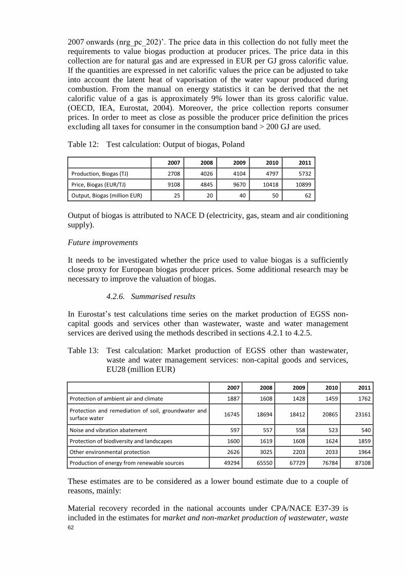
62
2007 onwards (nrg_pc_202)’. The price data in this collection do not fully meet the
requirements to value biogas production at producer prices. The price data in this
collection are for natural gas and are expressed in EUR per GJ gross calorific value.
If the quantities are expressed in net calorific values the price can be adjusted to take
into account the latent heat of vaporisation of the water vapour produced during
combustion. From the manual on energy statistics it can be derived that the net
calorific value of a gas is approximately 9% lower than its gross calorific value.
(OECD, IEA, Eurostat, 2004). Moreover, the price collection reports consumer
prices. In order to meet as close as possible the producer price definition the prices
excluding all taxes for consumer in the consumption band > 200 GJ are used.
Table 12: Test calculation: Output of biogas, Poland
2007 2008 2009 2010 2011
Production, Biogas (TJ) 2708 4026 4104 4797 5732
Price, Biogas (EUR/TJ) 9108 4845 9670 10418 10899
Output, Biogas (million EUR) 25 20 40 50 62
Output of biogas is attributed to NACE D (electricity, gas, steam and air conditioning
supply).
Future improvements
It needs to be investigated whether the price used to value biogas is a sufficiently
close proxy for European biogas producer prices. Some additional research may be
necessary to improve the valuation of biogas.
4.2.6. Summarised results
In Eurostat’s test calculations time series on the market production of EGSS non-
capital goods and services other than wastewater, waste and water management
services are derived using the methods described in sections 4.2.1 to 4.2.5.
Table 13: Test calculation: Market production of EGSS other than wastewater,
waste and water management services: non-capital goods and services,
EU28 (million EUR)
2007 2008 2009 2010 2011
Protection of ambient air and climate 1887 1608 1428 1459 1762
Protection and remediation of soil, groundwater and surface water
16745 18694 18412 20865 23161
Noise and vibration abatement 597 557 558 523 540
Protection of biodiversity and landscapes 1600 1619 1608 1624 1859
Other environmental protection 2626 3025 2203 2033 1964
Production of energy from renewable sources 49294 65550 67729 76784 87108
These estimates are to be considered as a lower bound estimate due to a couple of
reasons, mainly:
Material recovery recorded in the national accounts under CPA/NACE E37-39 is
included in the estimates for market and non-market production of wastewater, waste

63
and water management services as part of CEPA 3 (see section 4.1.1.). However,
any material recovery not recorded under national accounts’ CPA/NACE E37-39 is
not included in the test calculations.
The demand side data may not fully cover all fees and purchases for EP. For
example, if data on household expenditure in this source are missing some EGSS
output are consequently not (exhaustively) covered such as the operation and
maintenance of air pollution control devices for motor vehicles, sewage treatment
facilities such as septic tanks and chemicals to operate them, goods used in
connection with waste management such as bins, bags, composters etc. or low air
emission cars or eco-tourism.
The part of household production of energy that is not delivered to the electricity grid
(e.g. heating energy produced by geo thermal or solar thermal installations in private
dwellings for own-consumption) is not accounted for in the national accounts. Extra
efforts are therefore needed to include this output in the estimates of the production
of energy from renewable sources.
4.3. Market production of EGSS: capital goods and services
For estimating the production of EGSS capital goods and services supply side
sources such as SBS and PRODCOM may be used. The production of EGSS capital
goods and services may, however, also be identified using demand side data on gross
fixed capital formation (investments).
This practical guide proposes the demand side approach. Environmental investment
expenditure data are available for EP activities from the JQ-EPER. For RM national
accounts investment data are combined with other data sources such as energy
statistics or information from specific studies.
4.3.1. Demand side approach for environmental protection: capital
goods and services
This practical guide proposes to calculate output of EGSS capital goods and services
for EP using demand side data on investments from the JQ-EPER dataset. Investment
expenditure includes all outlays in a given year (purchases and own-account
production) for machinery, equipment, plant, buildings and land used for
environmental protection purposes. Total investments in a sector or industry are the
sum of two categories: (1) end-of-pipe investments (or pollution treatment
investments47
) and (2) investments in integrated technologies (or pollution
prevention investments48
).
For the purpose of the EGSS module investment expenditure from the JQ-EPER
broken down by environmental activities and industries must be mapped to the
producing NACE industries. It is proposed to use national account data on gross
fixed capital formation (investment) cross-classified by industries and types of asset
for this mapping.
47
for the collection and removal of pollutants (e.g. air emissions, effluents or solid waste), for the
prevention of the spread of pollution, for the measurement of the level of the pollution
48 modified or adapted production processes
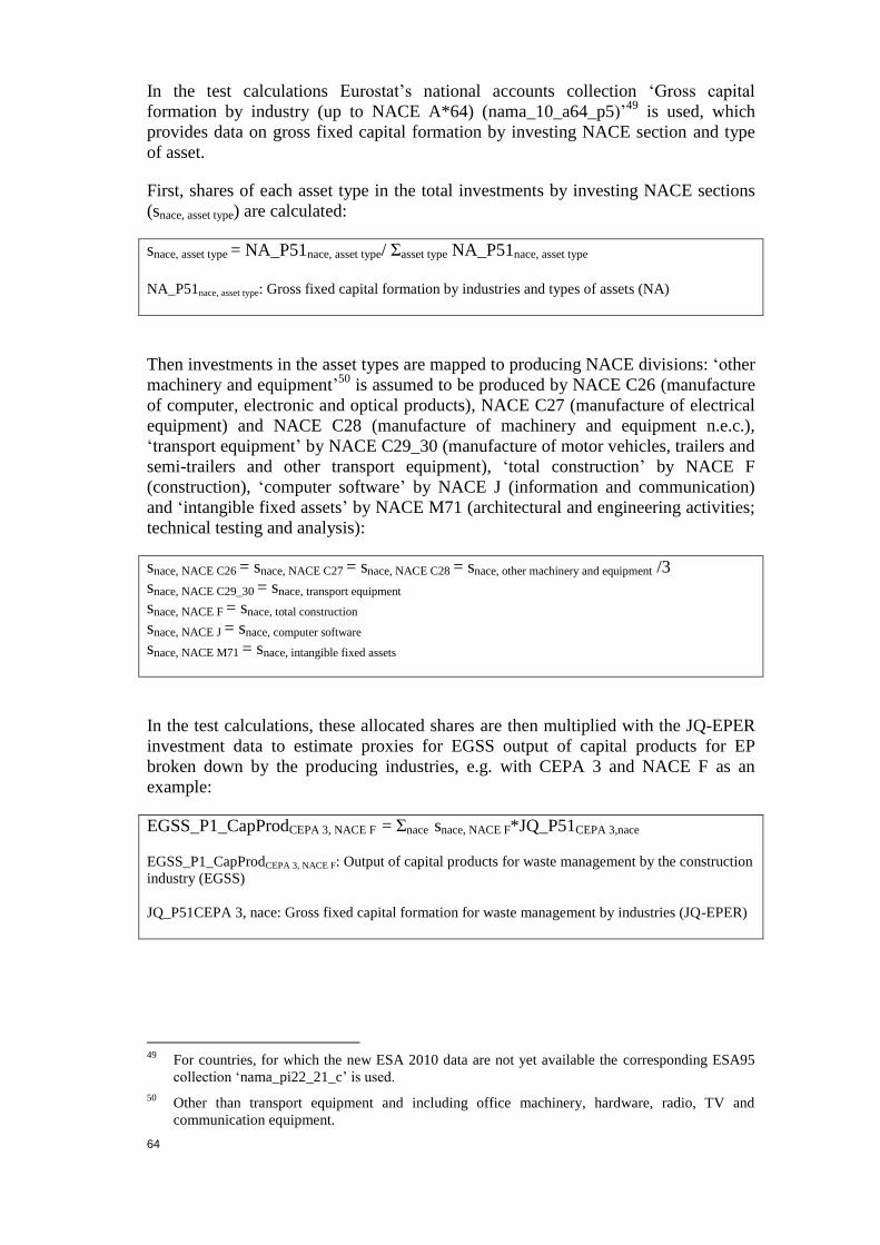
64
In the test calculations Eurostat’s national accounts collection ‘Gross capital
formation by industry (up to NACE A*64) (nama_10_a64_p5)’49
is used, which
provides data on gross fixed capital formation by investing NACE section and type
of asset.
First, shares of each asset type in the total investments by investing NACE sections
(snace, asset type) are calculated:
snace, asset type = NA_P51nace, asset type/ Σasset type NA_P51nace, asset type
NA_P51nace, asset type: Gross fixed capital formation by industries and types of assets (NA)
Then investments in the asset types are mapped to producing NACE divisions: ‘other
machinery and equipment’50
is assumed to be produced by NACE C26 (manufacture
of computer, electronic and optical products), NACE C27 (manufacture of electrical
equipment) and NACE C28 (manufacture of machinery and equipment n.e.c.),
‘transport equipment’ by NACE C29_30 (manufacture of motor vehicles, trailers and
semi-trailers and other transport equipment), ‘total construction’ by NACE F
(construction), ‘computer software’ by NACE J (information and communication)
and ‘intangible fixed assets’ by NACE M71 (architectural and engineering activities;
technical testing and analysis):
snace, NACE C26 = snace, NACE C27 = snace, NACE C28 = snace, other machinery and equipment /3
snace, NACE C29_30 = snace, transport equipment
snace, NACE F = snace, total construction
snace, NACE J = snace, computer software
snace, NACE M71 = snace, intangible fixed assets
In the test calculations, these allocated shares are then multiplied with the JQ-EPER
investment data to estimate proxies for EGSS output of capital products for EP
broken down by the producing industries, e.g. with CEPA 3 and NACE F as an
example:
EGSS_P1_CapProdCEPA 3, NACE F = Σnace snace, NACE F*JQ_P51CEPA 3,nace
EGSS_P1_CapProdCEPA 3, NACE F: Output of capital products for waste management by the construction
industry (EGSS)
JQ_P51CEPA 3, nace: Gross fixed capital formation for waste management by industries (JQ-EPER)
49
For countries, for which the new ESA 2010 data are not yet available the corresponding ESA95
collection ‘nama_pi22_21_c’ is used.
50 Other than transport equipment and including office machinery, hardware, radio, TV and
communication equipment.

65
This approach implicitly assumes that the investment structure by type of asset of a
NACE section as derived from national accounts also applies to the investments in
environmental protection for this NACE section.
An issue that is not reflected by the use of investment data is that of upstream links.
A producer satisfying the final demand for an EGSS product may use upstream
EGSS products produced by another EGSS producer as a component of his own
product (e.g. parts of hydraulic turbines delivered by a component producer to a
hydraulic turbine producer). Following the concepts of national accounts also the
upstream EGSS output should be accounted for. Without accounting the upstream
EGSS output EGGS employment estimates that would be based on demand side data
could systematically underestimate the number of direct employment in EGSS.
However, accounting for such upstream links is not a trivial task because, firstly, the
production chains within the EGSS are not easy to identify on the basis of existing
statistical data and, secondly, such upstream links may exist in practice over several
steps.
For the test calculations, an attempt has been made to derive estimates of the first
round upstream links using the national accounts use tables available in Eurostat’s
collection ‘Use table - current prices (NACE Rev. 2) (naio_cp16_r2)’. These use
tables provide information on intermediate inputs by 64 CPA product categories used
in the production of 64 NACE industries. The data on the main diagonal of the
64x64-matrix inform on the intermediate use of a CPA product within the same
characteristic industry, e.g. NA_P2CPA C28, NACE C28 would be the intermediate
consumption of product CPA C28 (machinery and equipment) in industry NACE 28
(manufacturing of machinery and equipment). This is considered as the value of
(components of) machinery delivered as upstream products to the machinery
manufacturing industry. These diagonal elements can be related to the total output of
the respective industry to derive multipliers (m) for the first round upstream link in
EGSS production, e.g. with NACE C28 as an example:
mNACE C28 = NA_P2CPA C28, NACE C28/ΣcpaNA_P1cpa, NACE C28 + 1
NA_P2CPA C28, NACE C28: Intermediate consumption of CPA product C28 by industry C28 (national
accounts - use table)
NA_P1cpa, NACE C28: Output of industry C28 by CPA products (national accounts - supply table).
Table 14: Test calculation: First round multipliers (m) for upstream links in EGSS
production, Czech Republic, selected industries
NACE 2007 2008 2009 2010 2011
C28 1.123 1.040 1.054 1.054 1.053
F 1.343 1.368 1.371 1.372 1.376
J 1.275 1.304 1.328 1.314 1.319
M71 1.108 1.156 1.174 1.181 1.192
For example, in table 14 the factor 1.123 for NACE C28 means that 1 € of final
expenditure on products produced by NACE C28 has an additional output impact on
NACE C28 of approximately 0.12 € due to the production of upstream output (CPA
C28 products used as components in the production by NACE C28). Applying the
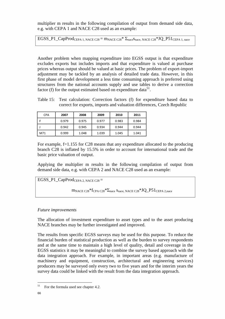
66
multiplier m results in the following compilation of output from demand side data,
e.g. with CEPA 1 and NACE C28 used as an example:
EGSS_P1_CapProdCEPA 1, NACE C28 = mNACE C28* Σnacesnace, NACE C28*JQ_P51CEPA 1, nace
Another problem when mapping expenditure into EGSS output is that expenditure
excludes exports but includes imports and that expenditure is valued at purchase
prices whereas output should be valued at basic prices. The problem of export-import
adjustment may be tackled by an analysis of detailed trade data. However, in this
first phase of model development a less time consuming approach is preferred using
structures from the national accounts supply and use tables to derive a correction
factor (f) for the output estimated based on expenditure data51
.
Table 15: Test calculation: Correction factors (f) for expenditure based data to
correct for exports, imports and valuation differences, Czech Republic
CPA 2007 2008 2009 2010 2011
F 0.979 0.975 0.977 0.983 0.984
J 0.942 0.945 0.934 0.944 0.944
M71 0.999 1.048 1.039 1.045 1.041
For example, f=1.155 for C28 means that any expenditure allocated to the producing
branch C28 is inflated by 15.5% in order to account for international trade and the
basic price valuation of output.
Applying the multiplier m results in the following compilation of output from
demand side data, e.g. with CEPA 2 and NACE C28 used as an example:
EGSS_P1_CapProdCEPA 2, NACE C28 =
mNACE C28*fCPA C28*Σnace snace, NACE C28*JQ_P51CEPA 2,nace
Future improvements
The allocation of investment expenditure to asset types and to the asset producing
NACE branches may be further investigated and improved.
The results from specific EGSS surveys may be used for this purpose. To reduce the
financial burden of statistical production as well as the burden to survey respondents
and at the same time to maintain a high level of quality, detail and coverage in the
EGSS statistics it may be meaningful to combine the survey based approach with the
data integration approach. For example, in important areas (e.g. manufacture of
machinery and equipment, construction, architectural and engineering services)
producers may be surveyed only every two to five years and for the interim years the
survey data could be linked with the result from the data integration approach.
51
For the formula used see chapter 4.2.

67
The first round multipliers (m) and the correction factors (f) for international trade
and valuation differences may need further investigation. In particular, multipliers
and correction factors based on NACE/CPA aggregates may not be sufficiently
representative for EGSS producers within these industries.
4.3.2. Demand side approach for water management: capital goods and
services
To estimate EGSS capital products for water management a demand side approach is
proposed using data from national accounts on gross fixed capital formation
(investment) cross-classified by industries and types of asset and output by industry.
The basic assumption is that the water supply industry is a mature industry that
shows a relatively stable relationship between investment and output in the longer
run.
For the test calculations, Eurostat’s collection ‘Gross capital formation by industry
(up to NACE A*64) (nama_10_a64_p5)’52
provides data on gross fixed capital
formation by type of asset and investing NACE section. The NACE section mainly
relevant for water management is section E (water supply, sewerage, waste
management and remediation activities). This information can be combined with
output data (NA_P1) from the collection ‘National Accounts aggregates by industry
(up to NACE A*64) (nama_10_a64)’53
to estimate investment factors per unit of
output for section E by type of asset (iasset type):
iasset type = NA_P51NACE E,asset type/NA_P1NACE E
NA_P51NACE E,asset type: Gross fixed capital formation of NACE section E by type of asset (NA)
NA_P1NACE E: Output of NACE section E (NA)
These investment factors by type of asset, which are ratios between gross fixed
capital formation and output of NACE section E, are mapped to the asset producing
industries: ‘other machinery and equipment’ to NACE C26 (manufacture of
computer, electronic and optical products), NACE C27 (manufacture of electrical
equipment) and NACE C28 (manufacture of machinery and equipment n.e.c.),
‘transport equipment’ to NACE C29_30 (manufacture of motor vehicles, trailers and
semi-trailers and other transport equipment, ‘total construction’ to NACE F
(construction), ‘computer software’ to NACE J (information and communication)
and ‘intangible fixed assets’ to NACE M71 (architectural and engineering activities;
technical testing and analysis):
52
For countries, for which the new ESA 2010 data are not yet available the corresponding ESA95
collection ‘nama_pi22_21_c’ is used.
53 For countries, for which the new ESA 2010 data are not available collection ‘annual National
Accounts by 64 branches at current prices (nama_nace64_c)’ is used.

68
iNACE C26 = iNACE C27 = iNACE C28 = iother machinery and equipment / 3
iNACE C29_30 = itransport equipment
iNACE F = itotal construction
iNACE J = icomputer software
iNACE M71 = iintangible fixed assets
The now allocated investment factors are then multiplied with the EGSS output of
water management services to arrive at proxies for the output of capital products for
water management broken down by industries, e.g. for NACE F (construction) as an
example:
EGSS_P1_CapProdCReMA 10, NACE F = iNACE F * Σnace EGSS_P1_ServCReMA 10, nace
EGSS_P1_CapProdCReMA 10, NACE F: Output of capital products for the management of water by NACE
F (EGSS)
EGSS_P1_ServCReMA 10, nace: Output of water management services by industries (EGSS)
It is to be noted that the approach shown above implicitly assumes that the
investment factors obtained for NACE section E are also representative for water
management services produced in any other industry. In practice, however, the
production of water management services outside of NACE E should be very small.
In addition, for the test calculation, an attempt has been made to derive an estimate
for the first round upstream multipliers (m) and to calculate correction factors (f) to
take into account international trade and valuation differences (for details on the
multipliers and factors, see the description of the test calculations made for capital
products for environmental protection). Applying these multipliers and factors gives
the following formula:
EGSS_P1_CapProdCReMA 10, NACE F =
mNACE F * fCPA F * iNACE F * Σnace EGSS_P1_ServCReMA 10, nace
Future improvements
The first round multipliers (m) and the correction factors (f) for international trade
and valuation differences may need further investigation. In particular, multipliers
and correction factors based on NACE/CPA aggregates may not be representative for
EGSS producers within those NACE industries.
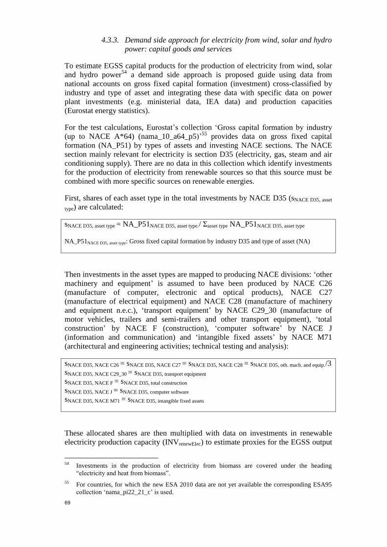
69
4.3.3. Demand side approach for electricity from wind, solar and hydro
power: capital goods and services
To estimate EGSS capital products for the production of electricity from wind, solar
and hydro power54
a demand side approach is proposed guide using data from
national accounts on gross fixed capital formation (investment) cross-classified by
industry and type of asset and integrating these data with specific data on power
plant investments (e.g. ministerial data, IEA data) and production capacities
(Eurostat energy statistics).
For the test calculations, Eurostat’s collection ‘Gross capital formation by industry
(up to NACE A*64) (nama_10_a64_p5)’55
provides data on gross fixed capital
formation (NA_P51) by types of assets and investing NACE sections. The NACE
section mainly relevant for electricity is section D35 (electricity, gas, steam and air
conditioning supply). There are no data in this collection which identify investments
for the production of electricity from renewable sources so that this source must be
combined with more specific sources on renewable energies.
First, shares of each asset type in the total investments by NACE D35 (sNACE D35, asset
type) are calculated:
sNACE D35, asset type = NA_P51NACE D35, asset type./ Σasset type NA_P51NACE D35, asset type
NA_P51NACE D35, asset type: Gross fixed capital formation by industry D35 and type of asset (NA)
Then investments in the asset types are mapped to producing NACE divisions: ‘other
machinery and equipment’ is assumed to have been produced by NACE C26
(manufacture of computer, electronic and optical products), NACE C27
(manufacture of electrical equipment) and NACE C28 (manufacture of machinery
and equipment n.e.c.), ‘transport equipment’ by NACE C29_30 (manufacture of
motor vehicles, trailers and semi-trailers and other transport equipment), ‘total
construction’ by NACE F (construction), ‘computer software’ by NACE J
(information and communication) and ‘intangible fixed assets’ by NACE M71
(architectural and engineering activities; technical testing and analysis):
sNACE D35, NACE C26 = sNACE D35, NACE C27 = sNACE D35, NACE C28 = sNACE D35, oth. mach. and equip./3
sNACE D35, NACE C29_30 = sNACE D35, transport equipment
sNACE D35, NACE F = sNACE D35, total construction
sNACE D35, NACE J = sNACE D35, computer software
sNACE D35, NACE M71 = sNACE D35, intangible fixed assets
These allocated shares are then multiplied with data on investments in renewable
electricity production capacity (INVrenewElec) to estimate proxies for the EGSS output
54
Investments in the production of electricity from biomass are covered under the heading
“electricity and heat from biomass”.
55 For countries, for which the new ESA 2010 data are not yet available the corresponding ESA95
collection ‘nama_pi22_21_c’ is used.

70
of capital products for renewable electricity production broken down by the
producing NACE branches, e.g. with NACE F (construction industry) used as an
example:
EGSS_P1_CapProdCReMA 13A, NACE F = sNACE D35, NACE F * INVrenewElec
EGSS_P1_CapProdCReMA 13A, NACE F: NACE F output of capital products for the production of
electricity from renewable sources (EGSS)
For the test calculation for Germany, the investment data for renewable electricity
production capacity are taken from publications on the website of the Federal
Ministry for environment, nature protection and nuclear safety56
. Any missing years
are estimated using ratios of ‘investments in renewable electricity production
capacity’ to positive57
year-on-year changes in renewable electricity production
capacity (main producers and auto-producers). These year-on-year changes are
derived from Eurostat’s collection ‘Infrastructure - electricity - annual data
(nrg_113a)’ taking into account capacities installed by main and auto-producers.
Both, the year-on-year changes and the investment data are shown in the following
two tables (below).
Table 16: Positive year-on-year changes in renewable electricity production
capacity, Germany (MW)
2007 2008 2009 2010 2011
Wind 1616 1633 1877 1509 1828
Hydro 38 0 690 0 218
Solar 1271 1950 4444 6988 7485
Table 17: Test calculation: Investments in renewable electricity production
capacity, Germany (million EUR)
2007 2008 2009 2010 2011
Wind 2276 2300 2650 2500 2950
Hydro 11 0 194 0 70
Solar 5211 7967 12000 19500 15000
Investments divided by the changes in renewable electricity production capacity (see
table below) are ratios that can be compared with sources on the investments costs
for newly installed capacities in order to check the plausibility of the used data.
“Overnight costs”58
for electric capacity from European on-shore wind power
56
Edler, Blazejczak, Wackerbauer, Rave, Legler, & Schasse (2009), Edler & Blazejczak, (2012),
Bundesministerium für Umwelt, Naturschutz und Reaktorsicherheit, (2012a), Bundesministerium
für Umwelt, Naturschutz und Reaktorsicherheit, 2012b, Bundesministerium für Umwelt,
Naturschutz und Reaktorsicherheit (2013)
57 Where year-to-year changes of the capacities are negative zero investments were assumed.
58 “Overnight costs” are the sum of pre-construction, construction and contingency costs. Data for
190 power stations in 21 countries have been published. Overnight costs data are available for the
following EU countries: Belgium (only on-shore wind), Czech Republic, France, Germany, Italy
and the Netherlands.
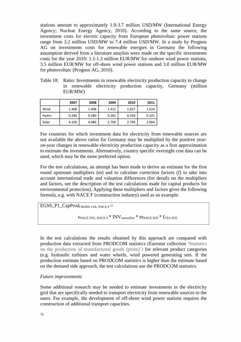
71
stations amount to approximately 1.9-3.7 million USD/MW (International Energy
Agency; Nuclear Energy Agency, 2010). According to the same source, the
investment costs for electric capacity from European photovoltaic power stations
range from 3.2 million USD/MW to 7.4 million USD/MW. In a study by Prognos
AG on investments costs for renewable energies in Germany the following
assumption derived from a literature anaylsis were made on the specific investments
costs for the year 2010: 1.1-1.3 million EUR/MW for onshore wind power stations,
3.5 million EUR/MW for off-shore wind power stations and 3.0 million EUR/MW
for photovoltaic (Prognos AG, 2010).
Table 18: Ratio: Investments in renewable electricity production capacity to change
in renewable electricity production capacity, Germany (million
EUR/MW)
2007 2008 2009 2010 2011
Wind 1.408 1.408 1.412 1.657 1.614
Hydro 0.280 0.280 0.281 0.330 0.321
Solar 4.100 4.086 2.700 2.790 2.004
For countries for which investment data for electricity from renewable sources are
not available the above ratios for Germany may be multiplied by the positive year-
on-year changes in renewable electricity production capacity as a first approximation
to estimate the investments. Alternatively, country specific overnight cost data can be
used, which may be the more preferred option.
For the test calculations, an attempt has been made to derive an estimate for the first
round upstream multipliers (m) and to calculate correction factors (f) to take into
account international trade and valuation differences (for details on the multipliers
and factors, see the description of the test calculations made for capital products for
environmental protection). Applying these multipliers and factors gives the following
formula, e.g. with NACE F (construction industry) used as an example:
EGSS_P1_CapProdCReMA 13A, NACE F =
sNACE D35, NACE F * INVrenewElec * mNACE D35 * fCPA D35
In the test calculations the results obtained by this approach are compared with
production data extracted from PRODCOM statistics (Eurostat collection ‘Statistics
on the production of manufactured goods (prom)’) for relevant product categories
(e.g. hydraulic turbines and water wheels, wind powered generating sets. If the
production estimate based on PRODCOM statistics is higher than the estimate based
on the demand side approach, the test calculations use the PRODCOM statistics.
Future improvements
Some additional research may be needed to estimate investments in the electricity
grid that are specifically needed to transport electricity from renewable sources to the
users. For example, the development of off-shore wind power stations requires the
construction of additional transport capacities.

72
The first round multipliers (m) and the correction factors (f) for international trade
and valuation differences may need further investigation. In particular, multipliers
and correction factors based on NACE/CPA aggregates may not be representative for
EGSS producers within those NACE industries.
4.3.4. Demand side approach for biofuels: capital goods and services
The estimate covers production plants to produce biofuels. To estimate EGSS capital
products for the production of biofuels a demand side approach is proposed by this
practical guide using data from national accounts on gross fixed capital formation
(investment) cross-classified by industry and type of asset and output by industry.
Eurostat’s collection ‘Gross capital formation by industry (up to NACE A*64)
(nama_10_a64_p5)’59
provides data on gross fixed capital formation by type of asset
and investing NACE sections. The NACE section mainly relevant for the production
of biofuels is section C (manufacturing). There are no data in this collection which
identify investments for the production of biofuels so that this source must be
combined with more specific sources on renewable energies.
First, shares of each asset type in the total investments by NACE C (sNACE C, asset type)
are calculated:
sNACE C, asset type = NA_P51NACE C, asset type./ Σasset type NA_P51NACE C, asset type
NA_P51NACE C, asset type: Gross fixed capital formation by industry C and type of asset (NA)
Then investments in the asset types are mapped to producing NACE divisions: ‘other
machinery and equipment’ is assumed to have been produced by NACE C26
(manufacture of computer, electronic and optical products), NACE C27
(manufacture of electrical equipment) and NACE C28 (manufacture of machinery
and equipment n.e.c.), ‘transport equipment’ by NACE C29_30 (manufacture of
motor vehicles, trailers and semi-trailers and other transport equipment, ‘total
construction’ by NACE F (construction), ‘computer software’ by NACE J
(information and communication) and ‘intangible fixed assets’ by NACE M71
(architectural and engineering activities; technical testing and analysis):
sNACE C, NACE C26=sNACE C, NACE C27=sNACE C, NACE C28 = sNACE C, other machinery and equipment /3
sNACE C, NACE C29_30 = sNACE C, transport equipment
sNACE C, NACE F = sNACE C, total construction
sNACE C, NACE J = sNACE C, computer software
sNACE D35, NACE M71 = sNACE D35, intangible fixed assets
In the test calculations, these allocated shares are then multiplied with data on
investments in biofuel production capacity (INVBiofuel) to estimate a proxy for the
59
For countries, for which the new ESA 2010 data are not yet available the corresponding ESA95
collection ‘nama_pi22_21_c’ is used.

73
EGSS output of capital products broken down by the producing NACE branches, e.g.
with NACE J (information and communication) used as an example:
EGSS_P1_CapProdCReMA 13A, NACE J = sNACE C, NACE J * INVBiofuel
EGSS_P1_CapProdCReMA 13A, NACE J: NACE J output of capital products for the production of biofuels
(EGSS)
INVBiofuel can be derived from the positive60
year-on-year changes of biofuel
capacities derived from Eurostat’s collection ‘Infrastructure - biofuel production
capacity - annual data (nrg_114a)’. The year-on-year changes are shown in the
following table (below). The changes in capacity are then multiplied with an estimate
of the investment costs per tonne61
.
Table 19: Positive year-to-year change in biofuel production capacities, Germany
(1000 t)
2007 2008 2009 2010 2011
322 254 1584 0 0
Table 20: Test calculation: Investments in biofuel production capacity, Germany
(million EUR)
2007 2008 2009 2010 2011
145 114 713 0 0
For the test calculation, an attempt has been made to derive an estimate for the first
round upstream multipliers (m) using the national accounts and to calculate
correction factors (f) to take into account international trade and valuation
differences (for details on the multipliers and factors, see the description of the test
calculations made for capital products for environmental protection). Applying these
multipliers and factors gives the following formula:
EGSS_P1_CapitalProductsCReMA 13A, NACE J =
sNACE C, NACE J * INVBiofuel * mNACE J * fCPA J
Future improvements
Additional research is needed to compile more reliable investment data for biofuel
production. The estimate of the investments as proposed above do not take into
account varying degrees of capacity utilisation, tear and wear of production
capacities and price changes for newly installed capital products. Also using data on
installed production capacity (if available) and its annual change could be a better
60
Where year-to-year changes of biofuel production were negative zero investments were assumed.
61 Based on a study carried out by Prognos AG ( 2010) it was assumed in the test calculations for
Germany that investment cost were 450 EUR/t

74
basis for the calculations than then used proxies derived from changes in biofuel
production.
The first round multipliers (m) and the correction factors (f) for international trade
and valuation differences may need further investigation. In particular, multipliers
and correction factors based on NACE/CPA aggregates may not be representative for
EGSS producers within those NACE industries.
4.3.5. Demand side approach for biogas: capital goods and services
To estimate EGSS capital products for the production of biogas a demand side
approach is proposed using data from national accounts on gross fixed capital
formation (investment) cross-classified by industry and type of asset and output by
industry.
For the test calculations, Eurostat’s collection ‘Gross capital formation by industry
(up to NACE A*64) (nama_10_a64_p5)’62
provides data on gross fixed capital
formation by type of asset and investing NACE sections. The NACE section mainly
relevant for the production of biofuels is section D35. There are no data in this
collection which identify investments for the production of biofuels so that this
source must be combined with more specific sources on renewable energies.
First, shares of each asset type in the total investments by NACE D35 (sNACE D35, asset
type) are calculated:
sNACE D35, asset type = NA_P51NACE D35, asset type./ Σasset type NA_P51NACE D35, asset type
NA_P51NACE D35, asset type: Gross fixed capital formation by industry D35 and type of asset (NA)
Then investments in the asset types are mapped to producing NACE divisions: ‘other
machinery and equipment’ is assumed to have been produced by NACE C26
(manufacture of computer, electronic and optical products), NACE C27
(manufacture of electrical equipment) and NACE C28 (manufacture of machinery
and equipment n.e.c.), ‘transport equipment’ by NACE C29_30 (manufacture of
motor vehicles, trailers and semi-trailers and other transport equipment), ‘total
construction’ by NACE F (construction), ‘computer software’ by NACE J
(information and communication) and ‘intangible fixed assets’ by NACE M71
(architectural and engineering activities; technical testing and analysis):
sNACE D35, NACE C26 = sNACE D35, NACE C27 = sNACE D35, NACE C28 = sNACE D35, oth. mach. and equip./3
sNACE D35, NACE C29_30 = sNACE D35, transport equipment
sNACE D35, NACE F = sNACE D35, total construction
sNACE D35, NACE J = sNACE D35, computer software
sNACE D35, NACE M71 = sNACE D35, intangible fixed assets
62
For countries, for which the new ESA 2010 data are not yet available the corresponding ESA95
collection ‘nama_pi22_21_c’ is used.
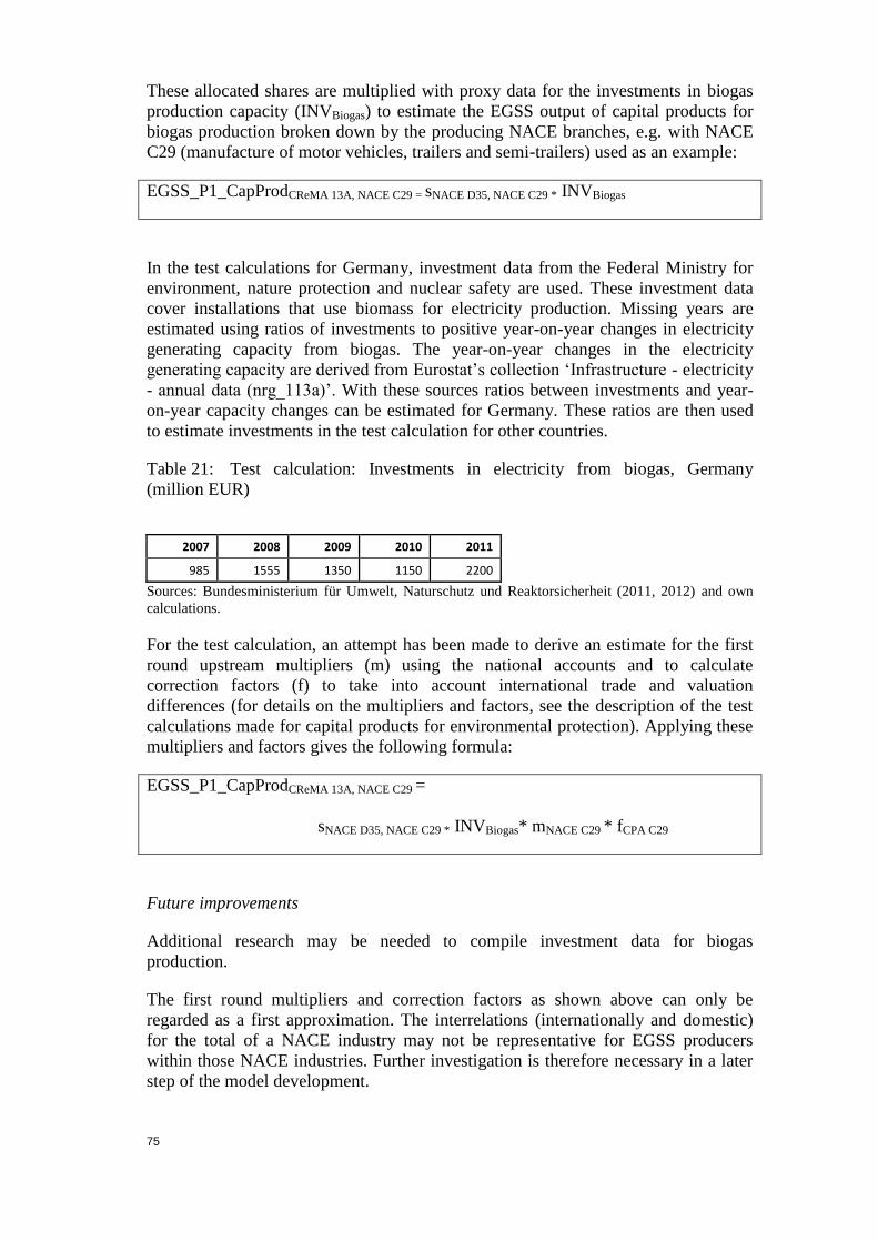
75
These allocated shares are multiplied with proxy data for the investments in biogas
production capacity (INVBiogas) to estimate the EGSS output of capital products for
biogas production broken down by the producing NACE branches, e.g. with NACE
C29 (manufacture of motor vehicles, trailers and semi-trailers) used as an example:
EGSS_P1_CapProdCReMA 13A, NACE C29 = sNACE D35, NACE C29 * INVBiogas
In the test calculations for Germany, investment data from the Federal Ministry for
environment, nature protection and nuclear safety are used. These investment data
cover installations that use biomass for electricity production. Missing years are
estimated using ratios of investments to positive year-on-year changes in electricity
generating capacity from biogas. The year-on-year changes in the electricity
generating capacity are derived from Eurostat’s collection ‘Infrastructure - electricity
- annual data (nrg_113a)’. With these sources ratios between investments and year-
on-year capacity changes can be estimated for Germany. These ratios are then used
to estimate investments in the test calculation for other countries.
Table 21: Test calculation: Investments in electricity from biogas, Germany
(million EUR)
2007 2008 2009 2010 2011
985 1555 1350 1150 2200
Sources: Bundesministerium für Umwelt, Naturschutz und Reaktorsicherheit (2011, 2012) and own
calculations.
For the test calculation, an attempt has been made to derive an estimate for the first
round upstream multipliers (m) using the national accounts and to calculate
correction factors (f) to take into account international trade and valuation
differences (for details on the multipliers and factors, see the description of the test
calculations made for capital products for environmental protection). Applying these
multipliers and factors gives the following formula:
EGSS_P1_CapProdCReMA 13A, NACE C29 =
sNACE D35, NACE C29 * INVBiogas* mNACE C29 * fCPA C29
Future improvements
Additional research may be needed to compile investment data for biogas
production.
The first round multipliers and correction factors as shown above can only be
regarded as a first approximation. The interrelations (internationally and domestic)
for the total of a NACE industry may not be representative for EGSS producers
within those NACE industries. Further investigation is therefore necessary in a later
step of the model development.

76
4.3.6. Demand side approach for heat and energy savings: capital
goods and services
To estimate EGSS capital products for heat and energy savings a demand side
approach is proposed by this practical guide using data from national accounts on
gross fixed capital formation (investment) cross-classified by industry and type of
asset as well as other sources such as specialised studies.
Eurostat’s collection “Cross-classification of gross fixed capital formation by
industry and by non-financial fixed asset - current prices (nama_pi22_21_c)”
provides data on gross fixed capital formation (NA_P51) in dwellings.
There are no statistical data on the share of energy and heat savings investments in
the total investments in dwellings. Some information may, however, be obtained
from specialised studies and agencies, for example:
From studies carried out by Naturschutzbund Deutschland (NABU) e.V. (2011)
and Deutsche Energieagentur (dena) (2010) it may be deducted that 30-40% of
all building investments in Germany were for the restoration of energetic
relevant parts of existing building and that around 30-50% of the investments in
energetic relevant parts were additional costs due to energy savings63
. These
ratios are based on a combination of market research data, statistical data, data
reported by participants of a low energy house restoration model project for the
years 2007 and 2009. If we combine this information it could be estimated that
around 10-20 % of all building investments were heat and energy saving
investments. Another study commissioned by Bundesministerium für Umwelt,
Naturschutz und Reaktorsicherheit (2013) mentions that gross investments in
buildings in the year 2005 amounted to EUR 197 billion in 2005 of which EUR
40 billion had an emission reducing impact, which is equivalent to a share of
20%. Information on data on subsidies and public loans for energetic renovation
can also be used to assess ratios and estimates of energy and heat savings
investments. The promotional KfW Bank Group joins the commercial banks in
the lending process and closes financing gaps to make the investment in energy-
efficient refurbishment or particularly energy-efficient houses affordable. KfW
data (KFW Bankengruppe, 2011 and KFW Bankengruppe, 2013) indicate that in
2010 a credit volume of EUR 5.2 billion was provided for energy efficient
refurbishment which had promoted investments of EUR 7.3 billion. For energy-
efficient construction a credit volume of EUR 3.7 billion had been provided with
a promoted investment of EUR 14.3 billion. KfW promoted investments in
energy-efficient refurbishment and energy efficient construction together
amounted to approximately 16% of total investments in dwellings in 2010
(2008: 10%, 2009: 15%, 2011: 13%64
). Based on this information for the test
63
The relatively wide range of this share (30-50%) depends on the energy saving standards to be
reached by the restoration measure. The Deutsche Energieagentur (dena) (2010) estimates that a
share of 30% would apply for restoration measures for the “Effzienzhaus 100”, whereas a share
of 50% would apply for measures to reach the “Effzienzhaus 55” standard. The numbers “55” and
“100” indicate the primary energy consumption of a house in percent of the primary energy
consumption of a reference building according to the German energy effciency decree
(Energieeffizienzverordnung – ENEV).
64 Data on total investments in dwellings are from national accounts data in Eurostat’s online
database.
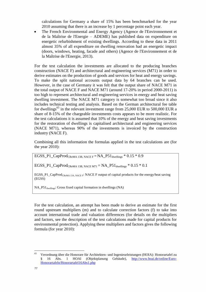
77
calculations for Germany a share of 15% has been benchmarked for the year
2010 assuming that there is an increase by 1 percentage point each year.
The French Environmental and Energy Agency (Agence de l'Environnement et
de la Maîtrise de l'Energie – ADEME) has published data on expenditure on
energetic refurbishment of existing dwellings. According to these data in 2011
almost 35% of all expenditure on dwelling renovation had an energetic impact
(doors, windows, heating, facade and others) (Agence de l'Environnement et de
la Maîtrise de l'Energie, 2013).
For the test calculation the investments are allocated to the producing branches
construction (NACE F) and architectural and engineering services (M71) in order to
derive estimates on the production of goods and services for heat and energy savings.
To make the split national accounts output data by 64 branches can be used.
However, in the case of Germany it was felt that the output share of NACE M71 in
the total output of NACE F and NACE M71 (around 17-20% in period 2000-2011) is
too high to represent architectural and engineering services in energy and heat saving
dwelling investment. The NACE M71 category is somewhat too broad since it also
includes technical testing and analysis. Based on the German architectural fee table
for dwellings65
in the relevant investment range from 25,000 EUR to 500,000 EUR a
share of 8-15% of the chargeable investments costs appears to be more realistic. For
the test calculations it is assumed that 10% of the energy and heat saving investments
for the restoration of dwellings is capitalised architectural and engineering services
(NACE M71), whereas 90% of the investments is invoiced by the construction
industry (NACE F).
Combining all this information the formulas applied in the test calculations are (for
the year 2010):
EGSS_P1_CapProdCReMA 13B, NACE F = NA_P51dwellings * 0.15 * 0.9
EGSS_P1_CapProdCReMA 13B, NACE M71 = NA_P51dwellings * 0.15 * 0.1
EGSS_P1_CapProdCReMA 13A, NACE F: NACE F output of capital products for the energy/heat saving
(EGSS) NA_P51dwellings: Gross fixed capital formation in dwellings (NA)
For the test calculation, an attempt has been made to derive an estimate for the first
round upstream multipliers (m) and to calculate correction factors (f) to take into
account international trade and valuation differences (for details on the multipliers
and factors, see the description of the test calculations made for capital products for
environmental protection). Applying these multipliers and factors gives the following
formula (for year 2010):
65
Verordnung über die Honorare für Architekten- und Ingenieurleistungen (HOIA): Honorartafel zu
§ 16 Abs. 1 HOAI (Objektplanung Gebäude), http://www.hoai.de/online/Euro-
Honorartafeln/Honorartafel16Abs1.php

78
EGSS_P1_CapProdCReMA 13B, NACE F = NA_P51dwellings*0.15*0.9*mNACE F*fCPA F
EGSS_P1_CapProdCReMA 13B, NACE M71 = NA_P51dwell.*0.15*0.1*mNACE M71*fCPA M71
Some methodological clarification is needed as concerns the estimate of building
materials for energy and heat saving investments (e.g. thermal insulation composite
systems). Such materials are normally invoiced by the construction companies to the
investors. In national accounts the purchase of such material by construction
companies is intermediate consumption. Therefore in the total output measure of the
economy the material is accounted twice as output of the industries that manufacture
the material and implicitly as part of the output of the construction industry. With a
view towards estimating also “green jobs” such upstream links should be accounted
for also in the EGSS module.
For energetic refurbishment the construction industries use capital goods that are
environmental goods (e.g. thermal insulating materials and equipment, heat
exchangers, heat pumps). These goods are mainly produced by the manufacturing
industry and mainly fall under the CPA categories C16 (products of wood and cork),
C22 (rubber and plastic products), C23 (non-metallic mineral products) and C28
(machinery and equipment).
The production of these goods may be determined using specific input coefficients
(i) for the construction industry:
EGSS_P1_CapProdCReMA 13B, NACE C23 =
EGSS_P1_CapProdCReMA 13B, NACE F * iCPA C23, NACE F * mNACE C23*fCPA C23
Potential sources to derive these specific input coefficients can be the systematic
analysis of invoices for refurbishment measures as well as expert knowledge
(engineering information). A first estimate of these coefficients may, however, also
be made by exploiting information available in the national accounts supply and use
tables. For Eurostat’s test calculations these input coefficients are calculated from the
supply and use tables.
A potential limitation of this approach is that the coefficients for the construction
industry as a total may not be representative for the energetic refurbishment activities
of that industry. Therefore the results obtained by this approach are compared with
production data extracted from PRODCOM statistics (Eurostat collection ‘Statistics
on the production of manufactured goods (prom)’) for relevant product categories
(e.g. multiple-walled insulating units of glass, heat pumps). If the production
estimate based on PRODCOM statistics is higher than the estimate based on the
supply and use tables (or if the latter cannot be produced because of missing data),
the test calculations use the PRODCOM statistics.
Future improvements
The Eurostat Task Force (TF) on the resource management expenditure account
(ReMEA) (Eurostat, 2013d) agreed on insulation as priority in the area of heat and
energy savings.

79
The estimate proposed in this practical guide is based on a share of heat and energy
saving investment for existing buildings in total building investments. Some research
may be necessary to find information for other countries and to regularly update the
shares over time. A way forward could be to use information on the production or
use of certain energy saving building materials (e.g. isolation material such as
mineral fibre) that could be used to develop a proxy for the dynamics in this area.
Refined estimation approaches may be based on data on subsidies paid by
governments for energetic renovation. Using subsidy data may, however,
underestimate energetic renovation for those parts of renovation for which investors
have – for various reasons – not received or asked for subsidies.
The first round multipliers (m) and the correction factors (f) for international trade
and valuation differences may need further investigation. In particular, multipliers
and correction factors based on NACE/CPA aggregates may not be representative for
EGSS producers within those NACE industries.
Other heat and energy saving investments such as energy saving modernisations of
buildings other than dwellings or the construction of new houses according to highest
energy savings standards are not yet taken into account. Practical experience exists
for heat and energy savings investments for new buildings, for example the
Netherlands uses a model that applies a cost factor to new dwellings (Eurostat,
2013d). Future research is necessary to define methods that are widely applicable to
other Member States, too.
4.3.7. Summarised results
In test calculations time series on the market production of EGSS capital goods and
services are derived using the methods described in the previous sections. Results at
aggregate EU level are shown below.

80
Table 22: Test calculations: Market production of EGSS: capital goods and services
by environmental activity, EU28 (million EUR)
CEPA/CreMA 2007 2008 2009 2010 2011
Protection of ambient air and climate 7582 8020 7374 7169 7358
Wastewater management 37527 39585 36287 34042 34653
Waste management 19951 20238 18480 18677 19551
Protection and remediation of soil, groundwater and surface water
2190 2328 2209 2303 2164
Noise and vibration abatement 1044 1128 1097 1037 911
Protection of biodiversity and landscapes 4798 4963 4939 4327 4455
Other environmental protection 2948 4333 3143 3229 3510
Management of water 5696 6731 5799 5034 5375
Energy from renewable sources 33835 49981 50063 62537 68060
Heat/energy savings and management 93445 97382 90188 98569 109067
Table 23: Test calculations: Market production of EGSS: capital goods and services
by economic activity, EU28 (million EUR)
NACE 2007 2008 2009 2010 2011
Total NACE
209014 234688 219579 236926 255105
of which:
C26 10345 13888 12068 13597 13521
C27 11624 14316 11960 15377 15016
C28 17417 21173 18436 23298 22930
F 126893 138008 133738 137402 153185
The estimate is to be considered as a lower bound estimate: Some important RM
activities are not yet covered such as the production of heat by solar thermal
installations and the minimisation of the intake of fossil resources as raw material.
4.4. Non-market production other than wastewater, waste and water management
services
This category covers all government EGSS output other than output of characteristic
environmental services. As a data source the JQ-EPER data for the public sector can
be used. Government EGSS output in characteristic environmental services
(wastewater management, waste management and water management) is not covered
in this category, but is estimated under the category ‘Market and non-market
(government) production of wastewater, waste and water management services’.
‘Internal current expenditure’ reported on the JQ-EPER should include the costs of
material used and compensation of employees for in-house environmental protection
activities, and exclude payments for bought environmental services.
Data on internal current expenditure on the following EP activities can be used:
protection of ambient air and climate (CEPA 1), protection and remediation of soil,
groundwater and surface water (CEPA 4), noise and vibration abatement (CEPA 5),

81
protection of biodiversity and landscapes (CEPA 6) and other environmental
protection activities (CEPA 7+8+9).
Since ‘Internal current expenditure’ reported on the JQ-EPER should only include
the costs of material used and compensation of employees for in-house
environmental protection activities, it conceptually produces a lower bound estimate
of government output. A complete valuation of government output from the cost side
would have to include the consumption of fixed capital. A simple approximation is to
estimate ratios of consumption of fixed capital to output from national accounts data
and to multiply them with the figures based on the JQ-EPER. In the test calculations,
in order to estimate the consumption of fixed capital by government activities NACE
specific ratios derived from Eurostat’s collection National Accounts aggregates by
industry (up to NACE A*64) (nama_10_a64)’66
are used.
In the table below results of the test calculations aggregated at EU level are shown.
Table 24: Test calculation: Non-market (government) production other than
wastewater, waste and water management services, EU28 (million EUR)
2007 2008 2009 2010 2011
Protection of ambient air and climate 1405 1237 1208 1072 1065
Protection of soil, groundwater, and surface water 1230 1228 1331 1240 1228
Noise and vibration abatement 823 824 855 752 772
Protection of biodiversity and landscapes 7297 7408 7713 7931 7979
Other environmental protection 10669 10569 10422 11138 11499
Further improvements
In the compilation framework developed so far all government (non-market) EGSS
output other than wastewater management, waste management and water
management is allocated to NACE section O (public administration and defence;
compulsory social security). Government finance statistics available at Eurostat do
not allow for a further breakdown of government expenditure by economic activity.
If a breakdown of government data by NACE is available at national level (e.g. data
available in the national account teams of the national statistical institutes) such data
should be used to improve the industry allocation.
Resource management activities are not covered by the JQ-EPER source. Future
developments of the resource management expenditure accounts (ReMEA) should
lead to improved data availability that may help to overcome data gaps for resource
management (Eurostat, 2013c).
4.5. Ancillary output
An ancillary activity is distinguished from principal and secondary activities in that
its output is only intended for use within the enterprise to enable the principal and
secondary activities to be carried out. Ancillary production of environmental services
is an internal activity of a producer unit (non-purchased from other units) that
66
For countries, for which the new ESA 2010 data were not available collection ‘annual National
Accounts by 64 branches at current prices (nama_nace64_c)’ is used.
82
produces services whose primary purpose is to protect the environment or natural
resources against the damaging or depleting impact of this unit’s activity.
In ESA (national accounts) all inputs consumed by ancillary activities are treated as
inputs to the production of principal and secondary output which they support.
Therefore output generated by ancillary activities is not a separately recorded output
category in ESA, but its value may be implicitly included in total output through the
application of the ESA valuation principles (basic prices or costs of production).
With the EGSS data collection questionnaire Eurostat asks Member States to
separately transmit data on ancillary output by EP activity and total output is defined
as including output of ancillary activities.
Internal production of environmental services for own use means that by definition
supply and demand are the same. Ancillary output therefore corresponds to the
producers’ inputs to the EGSS ancillary activities. These inputs comprise the use of
intermediate consumption, wages, and the consumption of fixed capital linked to the
production of ancillary output. Such information is normally not readily available in
existing bookkeeping systems and supply side oriented statistical data and it is
therefore recommended to use existing demand side sources.
For compiling ancillary output the data from JQ-EPER can be used. ‘Internal current
expenditure’ reported on the JQ_EPER should include the costs of material used and
compensation of employees for in-house environmental protection activities, and
exclude payments for bought environmental services.
The JQ-EPER provides numbers broken down by sector/industry and EP activities. It
distinguishes between the following types of sectors/industries:
PUBLIC SECTOR (government)
BUSINESS SECTOR TOTAL
o AGRICULTURE, FORESTRY AND FISHING
o MINING AND QUARRYING
o TOTAL MANUFACTURING
o ELECTRICITY, GAS, STEAM, AIR CONDITIONING SUPPLY; WATER
COLLECTION, TREATMENT AND SUPPLY
o OTHER BUSINESS
HOUSEHOLDS
PRIVATE & PUBLIC SPECIALISED PRODUCERS OF EP SERVICES
o PUBLIC SPECIALISED PRODUCERS OF EP SERVICES
o PRIVATE SPECIALISED PRODUCERS OF EP SERVICES
The JQ-EPER questionnaire foresees that expenditure by total manufacturing is
further broken down by nine groups of industries. This detail is filled in by most
countries.
The breakdown of the JQ-EPER by EP activities is not the same for all types of
sectors/industries: For all of them protection of ambient air and climate, wastewater
management and waste management are separately identified. In addition, for the
public sector, the business sector and the households, protection and remediation of

83
soil, groundwater and surface water, noise and vibration abatement and protection of
biodiversity and landscapes are separately covered by the questionnaire. An ‘other’
category allows entering figures for those remaining EP activities that are not
separately identified.
The Member States deliver annual data on the JQ-EPER. However, it may be
necessary to first gap-fill this dataset before using it for the compilation of the EGSS
module.67
It is to be noted that the estimation of ancillary EGSS output as part of total EGSS
output may result in some double counting if the ancillary activity serves a principal
or secondary activity to produce environmental goods and services; in theory, only
ancillary EGSS output used in the production of non-EGSS output should be taken
into account to avoid double counting. However, this distinction may be very
difficult to implement in surveys and other approaches to estimate the EGSS data,
and, in practice, the possible double counting is likely to be very tiny.
Some simplifying assumptions are made when calculating ancillary EGSS output
using the JQ-EPER:
To avoid double counting internal current expenditure by private and public
specialised producers of EP services is not counted towards ancillary output.
To avoid double counting with the other EGSS output of government (which is
calculated using the cost approach) internal current expenditure by the general
government is not counted towards ancillary output.
The JQ-EPER data for internal current expenditure (JQ_ICE) must be mapped to the
economic activities by 39 NACE categories (the same 39 categories as in the 2013
EGSS questionnaire). For example, the internal current expenditure for total
manufacturing may be distributed to the 13 manufacturing aggregates of the EGSS
using relative output shares based on national accounts data by 64 branches (Eurostat
collection ‘National Accounts aggregates by industry (up to NACE A*64)
(nama_10_a64)’68
’, e.g for CEPA 1 and NACE C26 used as an example:
EGSS_P1_AncCEPA 1, NACE C26 = JQ_ICECEPA 1, NACE C * NA_P1NACE C26/NA_P1NACE C
EGSS_P1_AncCEPA 1, NACE C26: Ancillary output of ambient air and climate protection in NACE C26
(EGSS)
JQ_ICECEPA 1, NACE C: Internal current expenditure on ambient air and climate protection by the
manufacturing industry (JQ-EPER)
NA_P1NACE C26: Output of manufacturing of computer, electronic and optical products (NA)
NA_P1NACE C: : Output of total manufacturing (NA)
67
For the purpose of calculating EU aggregates the gaps are filled by an approach developed by a
contractor to Eurostat over the recent years. However, the gap-filled dataset on environmental
protection expenditure is somewhat less detailed than the JQ-EPER: it does not include the type
‘other business’ and does not separate specialised producers into public and private producers.
68 For countries, for which the new ESA 2010 data were not available collection ‘annual National
Accounts by 64 branches at current prices (nama_nace64_c)’ has been used.

84
The results could be double checked against the detailed internal current expenditure
data of the manufacturing sector from the JQ-EPER.
Since ‘Internal current expenditure’ reported on the JQ-EPER should only include
the costs of material used and compensation of employees for in-house
environmental protection activities, it conceptually produces a lower bound estimate
of ancillary output of environmental protection services. A complete valuation of
ancillary output would have to include the consumption of fixed capital used for the
production of ancillary output as well as a component reflecting the net operating
surplus and mixed income. The gross operating surplus is the sum of these two
components. A simple approximation is to estimate ratios of gross operating surplus
to output (gop) from national accounts data on consumption of fixed capital
(NA_P51C) and net operating surplus and mixed income (NA_B2A3N) preferably
by an industry breakdown and to apply them to the figures based on the JQ-EPER,
e.g.:
EGSS_P1_AncCEPA 1, NACE C20 =
JQ_ICECEPA 1, NACE C * NA_P1NACE C20/NA_P1NACE C * (1+gopNACE C20)
with
gopNACE C20 = (NA_K1NACE C20 + NA_B2N_B3NACE C20) * NA_P1NACE C20
This approach assumes that the ratio gop as estimated for the totality of a NACE
industry is also applicable to the in-house environmental protection activities of that
industry.
In the test calculations, in order to estimate the gross operating surplus of ancillary
wastewater and waste management activities, ratios of gross operating surplus to
output of specialist sewerage and waste collection, waste treatment and waste
management producers (NACE E37-39) derived from Eurostat’s collection ‘National
Accounts aggregates by industry (up to NACE A*64) (nama_10_a64)’ are used, e.g.:
EGSS_P1_AncCEPA 2, NACE C26 =
JQ_ICECEPA 2, NACE C * NA_P1NACE C26/NA_P1NACE C * (1+gopNACE E37-39)
Table 25: Test calculation: ratios of gross operating surplus to output (gop) for
selected industries based on national accounts 64 industries breakdown,
Netherlands (%/100)
NACE 2007 2008 2009 2010 2011
C20 0.163 0.147 0.105 0.130 0.118
D 0.286 0.231 0.332 0.319 0.297
E36 0.398 0.381 0.384 0.389 0.377
O 0.174 0.172 0.166 0.171 0.178
In the table below results of the test calculations aggregated at EU level are shown.

85
Table 26: Test calculation: ancillary EGSS output by economic activity, EU28
(million EUR)
NACE 2007 2008 2009 2010 2011
Total NACE 19159 18598 18732 20744 21557
of which:
B 1451 1390 1180 1696 1494
C10-C12 1798 1704 1779 1871 1938
C22_C23 1027 942 894 959 1000
C24_C25 1876 1755 1456 1677 1819
C28 1293 1258 1150 1225 1319
C29_C30 1951 1749 1615 1885 1983
D 4009 4416 5464 5651 5967
Table 27: Test calculation: ancillary output of EGSS by environmental activity,
EU28 (million EUR)
CEPA 2007 2008 2009 2010 2011
Protection of ambient air and climate 5344 5278 4896 5559 5790
Wastewater management 5415 5636 6247 5932 6220
Waste management 4191 4191 3983 4170 4249
Protection and remediation of soil, groundwater and surface water
819 891 892 867 859
Noise and vibration abatement 502 481 562 854 530
Protection of biodiversity and landscape 737 658 682 715 994
Other environmental protection 2151 1463 1470 2647 2913
Further improvements
The gap-filled JQ-EPER dataset used in the test calculation does not include data on
internal current expenditure on environmental protection for NACE A and the
various service industries. If these data are available the internal current expenditure
for these industries can be mapped to ancillary output as well.
When countries report expenditure for the manufacturing industry in a more detailed
breakdown by nine groups of industries, the allocation of internal current expenditure
to the NACE groups may be improved. In particular it may be considered that most
probably those industries that have potentially strong negative impacts on the
environment have a relatively a high level of ancillary EP output in order to comply
with environmental laws.69
More specific information may be used to estimate the consumption of fixed capital
in ancillary environmental activities. At national level surveys may provide detailed
69
The results of the test calculation compared to the data transmitted with the JQ-EPER show that
in particular the estimate of ancillary output by the coke and refinery industry and the chemical
industry are likely to be underestimated when using simply national accounts output shares for
the distribution, whereas the ancillary output of other manufacturing industries are likely to be
overestimated.
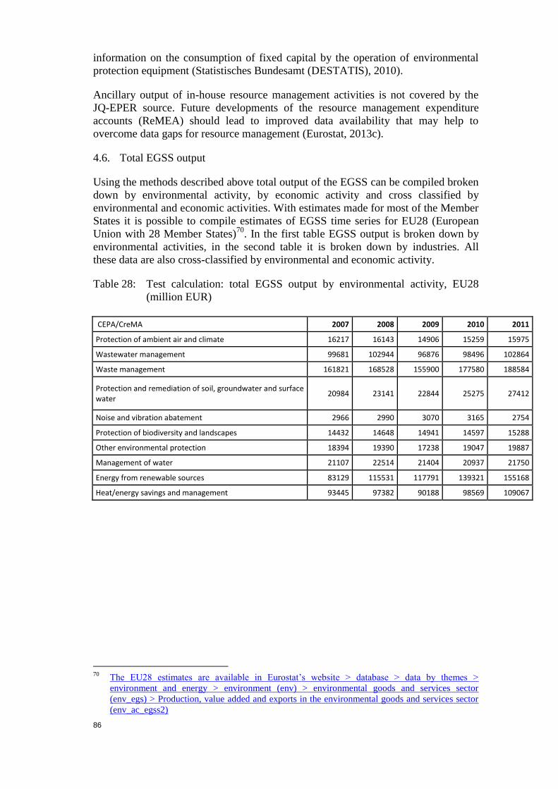
86
information on the consumption of fixed capital by the operation of environmental
protection equipment (Statistisches Bundesamt (DESTATIS), 2010).
Ancillary output of in-house resource management activities is not covered by the
JQ-EPER source. Future developments of the resource management expenditure
accounts (ReMEA) should lead to improved data availability that may help to
overcome data gaps for resource management (Eurostat, 2013c).
4.6. Total EGSS output
Using the methods described above total output of the EGSS can be compiled broken
down by environmental activity, by economic activity and cross classified by
environmental and economic activities. With estimates made for most of the Member
States it is possible to compile estimates of EGSS time series for EU28 (European
Union with 28 Member States)70
. In the first table EGSS output is broken down by
environmental activities, in the second table it is broken down by industries. All
these data are also cross-classified by environmental and economic activity.
Table 28: Test calculation: total EGSS output by environmental activity, EU28
(million EUR)
CEPA/CreMA 2007 2008 2009 2010 2011
Protection of ambient air and climate 16217 16143 14906 15259 15975
Wastewater management 99681 102944 96876 98496 102864
Waste management 161821 168528 155900 177580 188584
Protection and remediation of soil, groundwater and surface water
20984 23141 22844 25275 27412
Noise and vibration abatement 2966 2990 3070 3165 2754
Protection of biodiversity and landscapes 14432 14648 14941 14597 15288
Other environmental protection 18394 19390 17238 19047 19887
Management of water 21107 22514 21404 20937 21750
Energy from renewable sources 83129 115531 117791 139321 155168
Heat/energy savings and management 93445 97382 90188 98569 109067
70
The EU28 estimates are available in Eurostat’s website > database > data by themes >
environment and energy > environment (env) > environmental goods and services sector
(env_egs) > Production, value added and exports in the environmental goods and services sector
(env_ac_egss2)

87
Table 29: Test calculation: total EGSS output by industry, EU28 (million EUR)
NACE 2007 2008 2009 2010 2011
Total NACE
532176 583211 555159 612245 658748
of which:
A 15271 17269 17142 19546 21821
C26 11083 14531 12645 14256 14160
C27 12254 14933 12561 16037 15694
C28 18789 22515 19645 24592 24332
D 46141 58787 62547 68545 76341
E36 18876 19531 19242 19895 20647
E37 51104 51903 48681 52199 55608
E38 110506 115522 106571 122986 131469
E39 12278 12836 11841 13665 14608
F 127177 138296 134014 137689 153461
M71 16672 18112 17491 17993 20013
O 31851 32034 32335 33831 34463
The approach described in the previous sections has been tested for all Member
States of the EU except for Croatia. Largely, the same sources and approaches are
used for all countries. Therefore comparability of the estimates across countries is
relatively high.
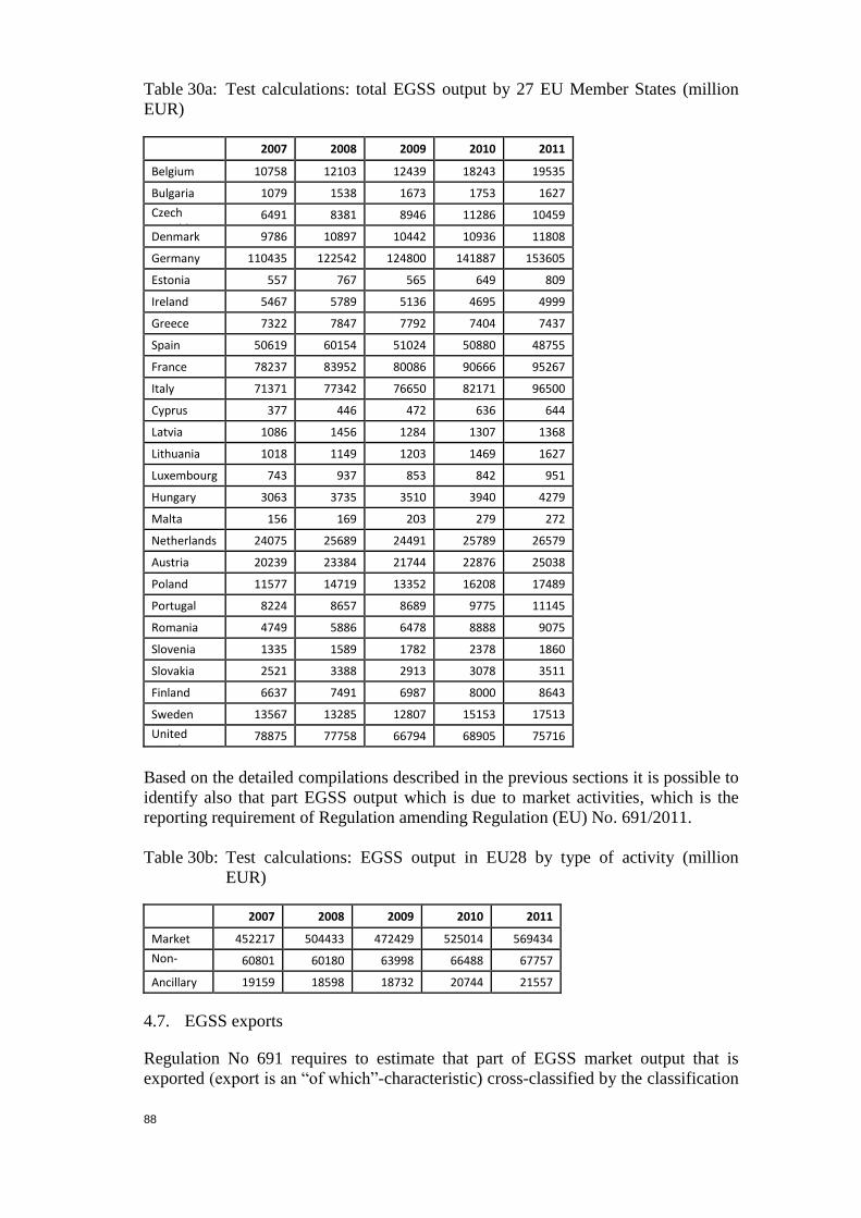
88
Table 30a: Test calculations: total EGSS output by 27 EU Member States (million
EUR)
2007 2008 2009 2010 2011
Belgium 10758 12103 12439 18243 19535
Bulgaria 1079 1538 1673 1753 1627
Czech Republic
6491 8381 8946 11286 10459
Denmark 9786 10897 10442 10936 11808
Germany 110435 122542 124800 141887 153605
Estonia 557 767 565 649 809
Ireland 5467 5789 5136 4695 4999
Greece 7322 7847 7792 7404 7437
Spain 50619 60154 51024 50880 48755
France 78237 83952 80086 90666 95267
Italy 71371 77342 76650 82171 96500
Cyprus 377 446 472 636 644
Latvia 1086 1456 1284 1307 1368
Lithuania 1018 1149 1203 1469 1627
Luxembourg 743 937 853 842 951
Hungary 3063 3735 3510 3940 4279
Malta 156 169 203 279 272
Netherlands 24075 25689 24491 25789 26579
Austria 20239 23384 21744 22876 25038
Poland 11577 14719 13352 16208 17489
Portugal 8224 8657 8689 9775 11145
Romania 4749 5886 6478 8888 9075
Slovenia 1335 1589 1782 2378 1860
Slovakia 2521 3388 2913 3078 3511
Finland 6637 7491 6987 8000 8643
Sweden 13567 13285 12807 15153 17513
United Kingdom
78875 77758 66794 68905 75716
Based on the detailed compilations described in the previous sections it is possible to
identify also that part EGSS output which is due to market activities, which is the
reporting requirement of Regulation amending Regulation (EU) No. 691/2011.
Table 30b: Test calculations: EGSS output in EU28 by type of activity (million
EUR)
2007 2008 2009 2010 2011
Market 452217 504433 472429 525014 569434
Non-market
60801 60180 63998 66488 67757
Ancillary 19159 18598 18732 20744 21557
4.7. EGSS exports
Regulation No 691 requires to estimate that part of EGSS market output that is
exported (export is an “of which”-characteristic) cross-classified by the classification
89
of economic activities and classes of the classifications of environmental activities
and resource management activities.
The required classification by NACE is a challenge since most available data sources
for trade are classified by products and not by economic activities: For example,
Eurostat disseminates detailed trade data according to the Combined Nomenclature
(CN8), whose first six digit codes coincide with the Harmonized Commodity
Description and Coding System (HS), whereas the Standard International Trade
Classification (SITC) or the Broad Economic Categories (BEC) is used for
aggregated data (Eurostat, 2013f). These classifications are classifications for
commodities (goods) and do not include services nor apply to economic activities71
.
Existing data sources
Trade in goods data can be downloaded from Eurostat’s on-line database collection
‘EU28 trade since 1988 by CN8 (DS_016890)’ or from Eurostat’s traditional
international trade database access (ComExt). Some examples of international trade
codes relevant for identifying envrionmental goods exports from the CN-8-digit-
classfication are shown in list 1 (see section 3.4). Some of the examples in this list
can be regarded as close to 100% EGSS goods (e.g. generating sets, wind powered –
CN 8502.31.00). Other codes of the CN-8-digit classification may include some
EGSS products but their share of EGSS would have to be determined using
additional information.
A source for trade in services is the balance of payment statistics. For example the
World Trade Organization publishes on its website data on exports of environmental
services derived from statistics on international service transactions. Balance of
payment (BoP) statistics provide information on international trade in services. These
data can be downloaded from Eurostat’s online database collection ‘International
trade in services (1985-2003) (bop_its_deth)’ and ‘International trade in services
(since 2004) (bop_its_det)’. For example, the BoP-code 282 for Waste treatment and
depollution includes the treatment of radioactive and other waste; stripping of
contaminated soil; cleaning up of pollution including oil spills; restoration of mining
sites; and decontamination and sanitation services. Also included are all other
services that relate to the cleaning or restoring of the environment. However, the
classification of services in the BoP (see metadata on international trade in services
statistics) is mostly not detailed enough to identify 100% environmental services so
that EGSS shares for the relevant codes would have to be estimated.
A source for exports broken down by economic activities is structural business
statistics (SBS). For example, statistical data on the manufacturing industry in
Germany (DESTATIS, 2014) contains data on foreign turnover (“Auslandsumsatz”).
Another source of relatively detailed data is the supply and use tables compiled in the
framework of the national accounts. Export data from the use tables are available in a
breakdown by CPA product codes which also includes goods and services. These
export data can be related to the output of the products in the supply tables. In the
Eurostat database the figures are available in a breakdown by 64 CPA categories.
71
Nomenclatures and correspondence tables are available from the Eurostat’s classification server
RAMON.

90
Calculating EGSS exports
If EGSS export data cannot be identified at a sufficiently detailed economic activity
breakdown, this practical guide recommends using sources that show export data
broken down by product classifications.
Where feasible it is recommended to use national accounts data since the
environmental accounts are a satellite of the national accounts. Using national
accounts data should ensure that the correct valuation method for EGSS exports is
used. For each CPA product of the national accounts’ supply and use tables the ratio
of exports to output can be calculated and multiplied with EGSS output in the
corresponding NACE activity (with CPA product E37 serving as an example in the
formula below):
EGSS_P7CEPA 2, NACE E37 =
EGSS_P1CEPA 2, NACE E37 * NA_P7CPA E37/ΣnaceNA_P1nace,CPA E37
EGSS_P7 CEPA 2,NACE E37: Exports of CEPA 2 products of industry NACE E37 (EGSS)
EGSS_P1 CEPA 2, NACE E37: Output of CEPA 2 products of industry NACE E37 (EGSS)
NA_P7CPA E37: Exports of product CPA E37 (national accounts use tables)
NA_P1nace, CPA E37: Output of product CPA E37 by industry (national accounts supply tables)
Behind the above formula stands the simplifying assumption that the exports share
for a CPA category is an indicator for the export shares of environmental goods and
services in the corresponding NACE category72
. This approach provides a first
estimate of EGSS exports by economic activity. It is expected to work fairly well for
industries with a high share of EGSS production (e.g. estimation of wastewater and
waste management services). However, if a more detailed product and activity
breakdown of the supply and use tables than A*64 is available using this more
detailed breakdown may be preferred.
Unfortunately, for industries with a very low share of EGSS production the approach
based on A*64 supply and use tables may not produce reliable results. An analysis
based on trade statistics is then to supplement this approach73
. As shown in list 1
72
The export shares also include exports and output produced as secondary output in NACE
categories other than the corresponding CPA category (e.g. CPA 37 produced by NACE 36).Such
a simplifying assumption has already been proposed for the calculation of EGSS output from
demand side data (see for example section 4.2.1).
73 Results of analyses of a limited number of trade codes relevant for environmental products have
been published in various studies commissioned by the European Commission (E.g. ECOTEC
(1999), Ernst & Young Environment and Sustainability Services (2006)).The ECORYS (2012)
study covering Brazil, China, EU27, India, Japan , Russia, USA and Canada analysed that the
EU27 share in exports of machines and equipment for air pollution control, hydropower,
environmental monitoring, photovoltaic, waste disposal and water pollution control amounted to
14% in 2010 (wherease its share in imports was 55%). The analysis of case studies (e.g. Steenblik
& Geloso Grosso, 2011) can help to enlarge existing trade codes lists for EGSS, to assess the
potential relevance of the various types of environmental services (e.g. business services, R&D,

91
(section 3.4) some trade codes are identifiable that correspond relatively closely to
EGSS goods.
Eurostat’s test calculations for EGSS exports are mainly based on the first approach
(i.e. using export shares by CPA category derived from national accounts supply and
use tables). However, for the exports of capital goods for the production of energy
from renewable sources (CreMA 13A) and energy savings (CreMA 13B) the results
obtained by this approach are compared with export data extracted from trade on
goods statistics for relevant product categories (mainly wind powered generating
sets, hydraulic turbines, photovoltaic cells, heat pumps, insulating units, multiple-
walled insulating glass). If exports based on trade on goods statistics are higher than
those based on the supply and use tables, the test calculations use the trade statistics.
Some additional collections from Eurostat’s international trade statistics
(‘International trade of EU, the euro area and the Member States by SITC product
group (ext_lt_intertrd)’) and from Eurostat’s data collections on the balance of
payments (‘Balance of payments by country’ (bop_q_c)) are used to complete the
trade data for goods and services.
Based on the test calculations for the Member States EU28 exports (extra-EU
exports) are estimated to amount to 6-8% of EGSS output
Linking the CN codes of the trade in goods statistics with the PRODCOM codes of
the ‘Statistics on the Production of Manufactured goods (prom)’ may also provide
relevant information on the export shares. In particular, if supply and use tables are
not available for all reporting years shares based on CN and PRODCOM codes may
be compiled to complete the times series.
Use of micro databases
For countries that have established a micro database on businesses active in the
production of envrionmental goods and services it may be possible to combine micro
data with trade in goods and services data by merging business identification
numbers to survey data on international trade so that environmental EGSS export
shares for individual trade codes can be determined. This approach may be
supplemented by expert guesses on EGSS specialisation of the businesses included in
the database (e.g. some businesses in the database may also produce and export non-
EGSS products). Sending out specifically designed questionnaires to collect data on
EGSS exports or additional questions to exisiting surveys can also be helpful for
identifying EGSS exports, shares of EGSS exports and specialisation factors if the
administrative and financial burden of doing so is acceptable. Limiting this burden
may be achieved by using survey data for benchmark years (e.g. for every third to
fifth reporting year) in order to calculate export shares and using interpolation
methods for years between two benchmarks.
Expert guesses
Some areas may depend heavily on expert guesses. For example, it is very difficult to
trace international trade in electricity from wind, hydro or photovoltaic power
because it is not a distinct product category in official classification systems for
computer related services, education services) that are exported and to assess the plausibility of
the results obtained by simpler methods.

92
trade. In such cases the above describve approach based on the supply and use tables
may also work as an alternative to expert guesses (e.g. with the basic assumption the
export share for total electricity output is an indicator for the export share for
renewable electricity output).

93
5. TEST CALCULATIONS FOR EGSS EMPLOYMENT
EGSS accounts report data on employment directly linked with the production of
EGSS output. Indirect employment due to the production of non-EGSS products
used as intermediate inputs for EGSS production should not be covered. A relatively
simple method to compile employment figures is to combine the estimates of EGSS
output by industry with national accounts data on wages and employment by
industry. Industry specific labour intensity coefficients can be multiplied with EGSS
output figures to estimate EGSS employment. This approach seems to be satisfactory
for all industries whose major part of production is in EGSS. However, the lower the
share of EGSS in total production of an industry, the bigger is the uncertainty about
the representativeness of the industries’ labour intensities for the EGSS. The
representativeness may then depend on the similarity between the technologies
applied in the production of EGSS and non-EGSS output within an industry. For
example, the labour intensity in the production of low air emission cars may be not
much different from the one in the production of normal cars, whereas different
technologies used in the production of electricity from renewable and non-renewable
sources may result in different intensities.
5.1. The basic model for estimating EGSS employment
The model for EGSS employment uses the same framework as the model for EGSS
output.
For better international comparison employment should be measured in full time
equivalent (FTE) rather than in number of persons employed. EGSS employment
broken down by industries and environmental activities is estimated from EGSS
output linked with national accounts information on the ratios between compensation
of employees and output (these ratios are called hereafter ‘c-ratios’) and labour
compensation rates per FTE (these ratios are called hereafter ‘w-ratios’):
EGSS_Empcepa/crema , nace = EGSS_P1 cepa/crema, nace * c-rationace / w-rationace
with:
c-rationace = NA_D1nace/NA_P1nace and w-rationace = NA_D1nace/FTEnace
EGSS_Empcepa/crema, nace: Employment cross-classified by industries and environmental activities
(EGSS)
EGSS_P1cepa/crema, nace: Output cross-classified by industries and environmental activities (EGSS)
NA_D1nace: Compensation of employees by industries (NA)
NA_P1nace: Output by industries (NA)
FTEnace: Employment by industries in full time equivalents
The basic assumption in this approach is that the average labour compensation rates
and intensities for an industry are sufficiently precise indicators for the EGSS
activities within the same industry. Some limitations of this basic assumption are

94
discussed below in sections 5.2. and 5.3 as well as proposals for refinement to
overcome some of the limitations (see also annex D).
The quotient of c- and w-ratios in the above formula could be replaced by the ratio
‘FTEnace/NA_P1nace‘. However, for plausibility checks of the data it is easier to
interpret the c- and w-ratios than directly the FTE to output ratio. Also, in case that
the employment data have gaps it is easier to estimate the c- and w-ratios separately
than to directly estimate their combined ratio.
In the following sections the compilation of the c- and w-ratios is described in more
detail.
5.2. Ratios: labour compensation to production value
Information on compensation of employees engaged in the production of EGSS
output is not readily available in existing statistical sources. A proxy for the ratio of
labour compensation to output (c-ratio) has therefore to be found. In the test
calculations ratios derived from national accounts data are used: Eurostat’s collection
on ‘National Accounts aggregates by industry (up to NACE A*64)
(nama_10_a64)’74
provides data on the compensation of employees and output from
which c-ratios for industries can be derived.
Table 31: Test calculations: ratios of labour compensation to output (c-ratios) for
selected industries and countries, year 2008
NACE Belgium Germany Italy Greece Slovakia Finland UK
A 0.263 0.361 0.344 0.635 0.524 0.546 0.172
B 0.160 0.272 0.114 0.368 0.205 0.144 0.079
C26 0.255 0.239 0.200 0.204 0.041 0.116 0.266
C27 0.280 0.264 0.154 0.139 0.147 0.178 0.283
C28 0.216 0.228 0.163 0.288 0.196 0.163 0.291
D 0.174 0.111 0.055 0.155 0.041 0.097 0.068
E36 0.318 0.210 0.206 0.420 0.309 0.181 0.164
E38 0.137 0.185 0.164 0.211 0.219 0.155 0.208
F 0.158 0.278 0.137 0.130 0.094 0.230 0.203
J 0.251 0.244 0.171 0.196 0.196 0.293 0.347
M69_M70 0.139 0.275 0.127 0.153 0.243 0.366 0.345
M71 0.240 0.314 0.098 0.112 0.158 0.370 0.387
M72 0.525 0.319 0.458 0.328 0.475 0.577 0.547
O 0.662 0.553 0.521 0.528 0.442 0.401 0.401
By using c-ratios derived from national accounts it is implicitly assumed that the
average compensation-output ratios for the single industries are representative for the
production of EGSS within these industries. This assumption may be justified by a
certain similarity of the processes and technologies used in the production of the
74
For countries, for which the new ESA 2010 data were not available collection ‘annual National
Accounts by 64 branches at current prices (nama_nace64_c)’ has been used.

95
goods and services within a given industry. C-ratios obtained from national accounts
for specific industries such as sewerage and waste management industries (which
mainly produce EGSS output) can be very good proxies.
On the other hand, for some EGSS producing industries c-ratios based on national
accounts data are less representative due to specific socio-economic conditions. For
example, agriculture has a very high share of self-employed persons and family
workers so that compensation of employees is less suitable to calculate the c-ratio.
Therefore, in the test calculation for Germany the c-ratios for agriculture are
estimated using bookkeeping data from the German Farm Accountancy Data
Network (Bundesministerium für Ernährung, Landwirtschaft und Verbraucherschutz,
2012a) on “income” and production value of organic farm holdings. The “income”
variable includes employees’ salaries and profits. The inclusion of profit in the
estimate of the c-ratio covers elements corresponding to the remuneration of work
carried out by the owners of the holdings and members of their families. A further
refinement of this approach would be to correct the income variable used to calculate
the c-ratio for the remuneration of capital and agricultural land to better represent
compensation of labour.
5.3. Ratios: labour compensation per full time equivalent
Information on labour compensation rates per FTE (w-ratios) in the EGSS is also not
readily available in existing statistical sources. Therefore also proxies for the w-
ratios need to be estimated. In the test calculations data on the compensation of
employees from Eurostat’s collection ‘National Accounts aggregates by industry (up
to NACE A*64) (nama_10_a64)’75
are used for most of the industries. This
information is combined with national accounts employment data from Eurostat’s
collection ‘National Accounts employment data by industry (up to NACE A*64)
(nama_10_a64_e)'76
, which provides statistical information on employment broken
down by employees and self-employed and measures employment in terms of hours
worked, number of jobs, number of persons and FTE. For the test calculation total
employment (employees plus self-employed) is used.
However, in this source employment data measured in FTE are often missing, so that
figures on the number of persons have to be converted. Given that part time work is a
widespread characteristic of working contracts using the number of employees
instead of FTE would probably result in some overestimation of the real
employment. Therefore a simple approach has been developed to convert the number
of employees using information on the share of part time work and hours worked.
This approach provides an estimate of FTE per person employed broken down by
industries. Using data from Eurostat data collections ‘Average number of usual
weekly hours of work in main job, by sex, professional status, full-time/part-time and
economic activity (from 2008 onwards, NACE Rev. 2) - hours (lfsa_ewhun2)’ and
‘Average number of usual weekly hours of work in main job, by sex, professional
status, full-time/part-time and economic activity (1983-2008, NACE Rev. 1.1) -
hours (lfsa_ewhuna)’ it is possible to calculate the ratios between hours worked per
employee in part time and in full time jobs (hereafter called ‘p-ratios’). From
75
For countries, for which the new ESA 2010 data are not available collection ‘annual National
Accounts by 64 branches at current prices (nama_nace64_c)’ is used.
76 Where the ESA 2010 collection was not available the corresponding ESA95 collection
‘nama_nace64_e’ was used.

96
Eurostat’s collection ‘Full-time and part-time employment by sex and economic
activity (from 2008 onwards, NACE Rev. 2) - 1 000 (lfsq_epgan2)’ and ‘Average
number of usual weekly hours of work in main job, by sex, professional status, full-
time/part-time and economic activity (1983-2008, NACE Rev. 1.1) - hours
(lfsa_ewhuna)’ it is possible to estimate ratios of the number of persons working
part-time to the total number of employees. Combining this information results in an
estimate of the FTE per employed person by economic activity:
FTEnace/employed personsnace =
part-time employmentnace/total employmentnace *(p-1) nace + 1
whereby 0 < p < 1
Analysing the above formula it becomes obvious that FTE per employed person
increases with a higher share of part time employment and a lower p-ratio (see also
table below).
Table 32: Full time equivalent (FTE) per employed person depending on the share
of part time employment and the ratio between hours worked per
employee in part time and in full time jobs (p-ratio), illustrative example
FTE per employed person Share of part time employment
in total employment p-ratio
1.000 0.0 any value
0.995 0.1 0.5
0.993 0.1 0.3
0.900 0.2 0.5
0.860 0.2 0.3
0.850 0.3 0.5
0.790 0.3 0.3
Based on the formula described above the ratios of FTE per employed person are
calculated for the NACE groups of the EGSS module.

97
Table 33: Test calculations: FTE per employed person for selected industries and
countries, year 2008
NACE Belgium Germany Italy Greece Slovakia Finland UK
A 0.924 0.845 0.942 0.922 0.987 0.874 0.857
B 1.000 0.966 0.976 1.000 1.000 1.000 0.962
C26 0.963 0.939 0.968 0.988 0.997 0.977 0.952
C27 0.963 0.939 0.968 0.988 0.997 0.977 0.952
C28 0.967 0.926 0.969 0.988 0.996 0.971 0.949
D 0.976 0.961 0.984 0.988 1.000 0.977 0.951
E36 0.974 0.937 0.946 0.977 0.879 0.977 0.952
E38 0.974 0.937 0.946 0.977 0.879 0.977 0.952
F 0.970 0.936 0.974 0.989 1.000 0.976 0.947
J 0.956 0.838 0.951 0.980 1.000 0.951 0.937
M69_M70 0.931 0.847 0.927 0.981 0.984 0.936 0.892
M71 0.931 0.847 0.927 0.981 0.984 0.936 0.892
M72 0.931 0.847 0.927 0.981 0.984 0.936 0.892
O 0.919 0.916 0.972 0.993 0.981 0.976 0.914
The w-ratios (labour compensation rates per FTE) can then be estimated using the
above mentioned national accounts data:
w-rationace = NA_D1nace/FTEnace =
(NA_D1nace/employed personsnace) / (FTEnace/employed personsnace)
Table 34: Test calculation: labour compensation per FTE (w-ratio) for selected
industries and countries, year 2008 (EUR)
NACE Belgium Germany Italy Greece Slovakia Finland UK
A 34699 33114 20751 15269 36189 27643 28988
B 51935 50076 42710 47725 13746 37188 78732
C26 72070 59253 41272 21999 10767 63280 50493
C27 58104 55462 35800 22185 10124 43804 50820
C28 58463 52225 42107 21478 13187 48060 50832
D 111804 59500 56596 51962 19614 55247 61060
E36 68032 47144 43991 37665 14430 33870 48871
E38 52581 38321 36128 38087 10369 35167 61898
F 35265 28601 19815 12206 7554 39045 28270
J 66897 53405 38746 31926 17242 51065 61556
M69_M70 19347 40820 14187 10373 10372 43301 37280
M71 41381 32627 10219 6779 11018 47601 41816
M72 83874 55391 56287 25858 12467 50612 61960
O 52566 44671 51442 32964 16570 41003 47135

98
As explained earlier in this chapter, the basic assumption of the estimation approach
is that the labour compensation rates and intensities in an industry are sufficiently
precise indicators for the EGSS activities within the same industry. The method
described above may therefore be supplemented by information that allows capturing
differences in the labour compensation rates and intensities. Such specific estimates
have been made for organic farming and the production of electricity from renewable
sources:
For organic farming in Germany the w-ratios are directly derived from the
aforementioned bookkeeping data from the German Farm Accountancy Data
Network (Bundesministerium für Ernährung, Landwirtschaft und
Verbraucherschutz, 2012a).
The generation of electricity from renewbale sources and non-renewable
sources are differnt in terms of labour input needed or operating and
maintenance (International Labour Organisation (ILO, 2013)). The test
calculations include mark-up factors for the w-ratios to reflect that operating
and maintenance costs (O&M) for electricity generation from renewable
sources can differ from those for electricity generation from non-renewable
sources. At international level data on O&M and levelised costs of electricity
(LCOE) by type of technology have been collected for 21 countries and 190
power plants (International Energy Agency; Nuclear Energy Agency, 2010).
Based on this source the mark-up factors can be calculated (for more details
see Annex D).
5.4. Results on EGSS employment
In combining all the calculation steps described above in sections 5.1 to 5.3 EGSS
direct employment by environmental activities and industries is compiled. With
estimates made for most of the Member States it possible to produce estimates of
EGSS time series for EU28 (European Union with 28 Member States)77
. In the first
table EGSS employment is broken down by environmental activities, in the second
table it is broken down by industries. All these data are also cross-classified by
environmental activities and industries.
77
The EU28 estimates are available in Eurostat’s website > database > data by themes >
environment and energy > environment (env) > environmental goods and services sector
(env_egs) > Employment in the environmental goods and services sector (env_ac_egss1)

99
Table 35: Test calculation: total EGSS employment by environmental activities,
EU28 (1000 FTE)
CEPA/CreMA 2007 2008 2009 2010 2011
Protection of ambient air and climate 111 109 113 98 102
Wastewater management 648 663 687 644 629
Waste management 957 999 1010 1062 1083
Protection and remediation of soil, groundwater and surface water
370 394 425 457 466
Noise and vibration abatement 25 24 25 22 21
Protection of biodiversity and landscapes 133 132 136 132 133
Other environmental protection 180 188 177 186 188
Management of water 146 154 147 142 144
Energy from renewable sources 324 446 523 596 647
Heat/energy savings and management 673 699 691 730 767
Table 36: Test calculation: total EGSS employment by industries, EU28 (1000
FTE)
NACE 2007 2008 2009 2010 2011
Total NACE 3568 3807 3934 4068 4181
of which:
A 320 346 377 411 422
C26 49 69 70 66 66
C27 68 81 83 89 81
C28 93 118 122 133 117
D 90 103 114 124 132
E36 152 152 154 158 159
E37 266 260 267 260 262
E38 570 595 607 647 670
E39 63 66 67 72 74
F 1034 1124 1190 1200 1264
M71 145 155 161 160 177
O 379 366 359 365 366
The approach described in the previous sections has been tested for all Member
States of the EU (except for Croatia) and results are shown in the following table.
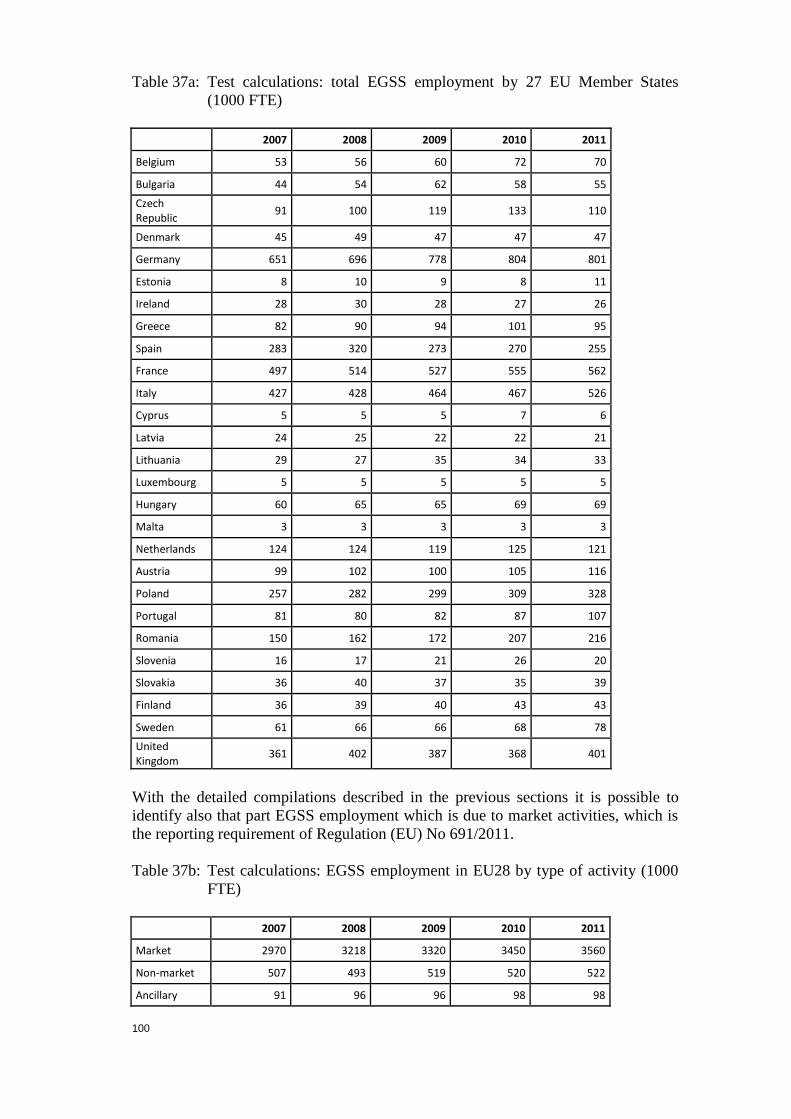
100
Table 37a: Test calculations: total EGSS employment by 27 EU Member States
(1000 FTE)
2007 2008 2009 2010 2011
Belgium 53 56 60 72 70
Bulgaria 44 54 62 58 55
Czech Republic
91 100 119 133 110
Denmark 45 49 47 47 47
Germany 651 696 778 804 801
Estonia 8 10 9 8 11
Ireland 28 30 28 27 26
Greece 82 90 94 101 95
Spain 283 320 273 270 255
France 497 514 527 555 562
Italy 427 428 464 467 526
Cyprus 5 5 5 7 6
Latvia 24 25 22 22 21
Lithuania 29 27 35 34 33
Luxembourg 5 5 5 5 5
Hungary 60 65 65 69 69
Malta 3 3 3 3 3
Netherlands 124 124 119 125 121
Austria 99 102 100 105 116
Poland 257 282 299 309 328
Portugal 81 80 82 87 107
Romania 150 162 172 207 216
Slovenia 16 17 21 26 20
Slovakia 36 40 37 35 39
Finland 36 39 40 43 43
Sweden 61 66 66 68 78
United Kingdom
361 402 387 368 401
With the detailed compilations described in the previous sections it is possible to
identify also that part EGSS employment which is due to market activities, which is
the reporting requirement of Regulation (EU) No 691/2011.
Table 37b: Test calculations: EGSS employment in EU28 by type of activity (1000
FTE)
2007 2008 2009 2010 2011
Market 2970 3218 3320 3450 3560
Non-market 507 493 519 520 522
Ancillary 91 96 96 98 98

101
5.5. Future improvements
Data on wage to output ratios and wages per employee or full time equivalents for a
certain industry may not always be a good proxy for EGSS related employment
within the same industry. Therefore additional information may be needed to
improve the estimates.
The results from specific surveys on EGSS that ask for the wages, number of
employees, full time equivalents may be used for this purpose. Survey approaches
are often considered to be the best method since existing classifications are not
structured to differentiate EGSS employment from other employment in the same
industries (see also section 3.2.1 for more details on using surveys). However,
surveys can be costly in terms of financial burden for statistical offices and burden
for respondents. To reduce the financial burden of statistical production as well as
the burden to survey respondents and at the same time to maintain a high level of
quality, detail and coverage in the EGSS statistics it may be meaningful to combine
the survey based approach with the data integration approach. For example, in some
areas (e.g. manufacture of machinery and equipment, construction, architectural and
engineering services) producers may be surveyed only every two to five years and
for the intermediate years the survey data could be linked with the result from the
data integration approach. Such an approach may significantly reduce the statistical
burden while maintaining a high level of statistical quality and detail in the EGSS
module.
Engineering analysis may also be useful to improve the employment estimates in
certain areas. For example, a study carried out by ECOTEC Research & Consulting
Limited (1999) for the Commission’s DG Environment provides information on the
breakdown of operating expenditure related to environmental protection by cost
categories (see Table 6). However before using such information it must be ensured
that conceptual differences are properly taken into account and that the information
is updated to reflect the most important technological and economic trends. By using
information on the ratios ‘gross operating surplus/output’ the ECOTEC ratios
‘wage/operating expenditure’ may be converted into proxies for ‘compensation of
employees/output’. For example, with a 40% share of gross operating surplus in
output the ECOTEC ratios would convert to ratios ‘compensation of
employees/output’ of approximately 0.3 for wastewater management and 0.4 for
waste management. By contrast, national accounts for Germany show that wage to
output ratios have strongly declined over the last 10 years, e.g. in NACE E37-39
from 0.23 in 2000 down to 0.17 in 2010.
Data on the production cost structure can be useful additional information to allow
for a better representation of EGSS specific conditions with respect to wages and
employment. An example for the use of such additional data for the EGSS
employment estimates is provided in annex D and has been implemented in the test
calculations for energy from renewable sources.

102
6. TEST CALCULATIONS FOR EGSS GROSS VALUE ADDED
6.1. The model for estimating EGSS gross value added
The model for EGSS gross valued added (GVA) uses the same framework as the
models for EGSS output and employment.
EGSS GVA broken down by industries and environmental activities is estimated
from EGSS output linked with national accounts information on the ratios between
gross valued added and output. Gross valued added covers compensation of
employees, net operating surplus and mixed income and the consumption of fixed
capital:
EGSS_B1Gcepa/crema, nace = EGSS_P1cepa/crema, nace *
(NA_D1nace+NA_B2NB3Nnace+NA_K1)/NA_P1nace
EGSS_B1Gcepa/crema, nace: Gross valued added cross-classified by industries and environmental
activities (EGSS)
EGSS_P1cepa/crema, nace: Output cross-classified by industries and environmental activities (EGSS)
NA_D1nace: Compensation of employees by industries (NA)
NA_B2NB3Nnace: Net operating surplus and net mixed income by industries (NA)
NA_K1nace: Consumption of fixed capital by industries (NA)
NA_P1nace: Output by industries (NA)
The basic assumption is that the average gross value added shares in output for an
industry are sufficiently precise indicators for the EGSS activities within the same
industry. The only exemption from this general rule is made in the test calculations
for Germany for the GVA of NACE A. Instead of the national accounts data on
compensation of labour and net operating surplus and mixed income the GVA
calculations for NACE A are based on an “income” variable derived from
bookkeeping data from the German Farm Accountancy Data Network. This
“income” variable includes employees’ salaries and profits in organic farming (see
section 5.2 for details). Consumption of fixed capital derived from national accounts
is added to obtain a proxy for the GVA in organic farming.
6.2. Results on EGSS gross value added
The approach described above to calculate EGSS GVA has been tested for all
Member States of the EU except for Croatia. With estimates made for most of the
Member States it is possible to produce estimates for EU28 (European Union with 28
Member States)78
.
78
The EU28 estimates are available in Eurostat’s website > database > data by themes >
environment and energy > environment (env) > environmental goods and services sector
(env_egs) > production, value added and exports in the environmental goods and services sector
(env_ac_egss2)

103
Table 38: Test calculation: total EGSS GVA by environmental activities, EU28
(million EUR)
CEPA/CreMA 2007 2008 2009 2010 2011
Protection of ambient air and climate 6612 6407 6122 6220 6402
Wastewater management 41182 42353 40716 40970 41558
Waste management 64334 67095 64631 71857 73690
Protection and remediation of soil, groundwater and surface water
14061 15046 15378 16618 17845
Noise and vibration abatement 1453 1457 1502 1592 1335
Protection of biodiversity and landscapes 7764 7964 8260 8156 8408
Other environmental protection 9967 10418 9500 10248 10707
Management of water 9644 10066 9583 9323 9711
Energy from renewable sources 28816 39190 42055 49329 52994
Heat/energy savings and management 36085 37515 35644 39030 42521
Table 39: Test calculation: total EGSS GVA by industries, EU28 (million EUR)
NACE 2007 2008 2009 2010 2011
Total NACE 219917 237512 233393 253343 265172
of which:
A 11402 12343 12682 13962 15249
C26 4004 5195 4732 5361 5276
C27 4156 5178 4527 5796 5414
C28 6401 7705 6942 8952 8586
D 15166 18655 21137 22907 24463
E36 9858 10015 9552 9759 10203
E37 21292 21715 20860 21688 22195
E38 42244 44185 42780 47792 48925
E39 4701 4923 4738 5310 5436
F 48230 52516 51938 53720 58749
M71 8868 9559 9363 9632 10730
O 20913 21045 21233 22171 22747
Relating EGSS GVA to GDP makes it possible to compare the results obtained for
the different countries.

104
Table 40a: Test calculations: total EGSS gross value added by 27 EU Member
States, 2011
2007 2009 2011
million EUR % of GDP million EUR % of GDP million EUR % of GDP
Belgium 4115 1.2 4718 1.3 6690 1.8
Bulgaria 321 1.0 518 1.4 564 1.4
Czech Republic
2320 1.7 3273 2.2 3701 2.3
Denmark 3948 1.7 4219 1.8 4764 1.9
Germany 48090 1.9 55335 2.3 64898 2.4
Estonia 232 1.4 229 1.6 330 2.0
Ireland 1806 0.9 1572 0.9 1559 0.9
Greece 5062 2.2 5651 2.4 4360 2.1
Spain 20113 1.9 22523 2.1 21858 2.0
France 33679 1.7 35499 1.8 39874 1.9
Italy 24392 1.5 28053 1.8 32378 2.0
Cyprus 189 1.1 219 1.2 287 1.5
Latvia 405 1.8 473 2.5 482 2.4
Lithuania 510 1.8 600 2.2 693 2.2
Luxembourg 318 0.9 372 1.0 406 1.0
Hungary 1219 1.2 1351 1.4 1588 1.6
Malta 84 1.5 98 1.6 116 1.7
Netherlands 10538 1.7 10588 1.7 11262 1.8
Austria 8371 3.0 8316 2.9 9847 3.2
Poland 4827 1.5 5740 1.8 7199 1.9
Portugal 2818 1.6 3156 1.8 3672 2.1
Romania 1859 1.5 2430 2.0 4017 3.0
Slovenia 525 1.5 697 1.9 680 1.8
Slovakia 1070 1.9 1200 1.9 1331 1.9
Finland 2815 1.5 2989 1.7 3525 1.8
Sweden 5936 1.7 5680 1.8 7812 1.9
United Kingdom
33605 1.6 27034 1.6 30379 1.6

105
With the detailed compilations explained in the previous sections it is possible to
identify also that part EGSS GVA which is due to market activities, which is the
reporting requirement of Regulation (EU) No 691/2011.
Table 40b: Test calculations: EGSS GVA in EU28 by type of activity (million EUR)
2007 2008 2009 2010 2011
Market 180975 199247 193163 211012 222759
Non-market 32467 32176 33894 35185 35386
Ancillary 6475 6089 6335 7146 7027
106
ANNEX A: PROBLEMS RELATED TO THE CATEGORISATION OF ENVIRONMENTAL
PRODUCTS
The categories of environmental products are defined partly with reference to the
technology concept from research, development and innovation statistics and partly
with reference to categories of goods and services (Eurostat, 2013b). In practice,
EGSS statistics are usually compiled with reference to lists of goods and services and
the EGSS technologies category is used to track the production and installation of
certain investment products that are combined into items of investment (e.g.
machinery, components, construction works, architectural and installation services
which are combined to form a wind mill park). Some environmental technologies
may be included in the categories of connected products or adapted goods, and there
may be products that are at the same time connected and adapted goods (e.g. a
biodegradable trash-bag). For such cases it is important to have a list of products that
exclusively relates them to one of the different product categories.
Some further delimitation problems for cleaner goods and cleaner technologies are
presented in greater detail in the box below:
Is a “cleaner good” or “cleaner technology” (adapted goods and integrated
technologies) cleaner?
The definition of “cleaner” poses measurement challenges because many goods and
technologies produced or applied today are less polluting or less resource depleting than in
the past (e.g. practically all motor vehicle engines fabricated today produce less air
emissions and use less fuel than those engines of the same power produced 10 years ago). A
good or a technology that is leading in terms of cleanness today may not be cleaner than the
average of the goods and technologies of the same type in five years.
Also the production of integrated technology and adapted goods and of the inputs used to
operate them may result in environmental pollution or resource depletion. For example, for
a low air emission vehicle to be recorded under CEPA 1 (protection of ambient air and
climate) the car must be less polluting when used or scrapped than equivalent normal cars
which furnish a similar utility. This criterion, however, does not take into account the
pollution caused by the manufacturer of the car nor does it consider, in the case of an
electric car, the emissions resulting from the production of the electricity used to operate the
car (Eurostat, 2012a) (p. 7).
Conventional production technologies or conventional goods may be no more polluting
than integrated technologies and adapted goods if effective end-of-pipe technologies are
installed to treat emissions or to scrap, reutilize or recycle the goods at the end of their life
cycles without release of dangerous substances into the environment.
Is organic farming an integrated technology or the production of adapted goods?
Organic farming is said to be an integrated technology in the 2009 EGSS handbook.
However, when calculating the production value of the EGSS, there is unlikely to be any
production of this technology. Therefore, organically produced agricultural products are,
according to the EGSS handbook (p.55), considered as adapted goods, although the output
from organic farming is not itself an environmental good that will enable someone to
improve the environment.
Definitions used in the environmental protection expenditure accounts (EPEA) often
differ from those in EGSS although the same terminology is used. In particular the
scope and measurement of adapted goods and technologies are different in the two

107
environmental accounts domains. Such consistency problems between EPEA and
EGSS are presented in greater detail in the box below:
The scope and measurement of adapted goods and integrated technologies in EGSS
differs from that in the EPEA:
Whereas in EGSS technologies are seen as product categories distinct from connected and
adapted goods, in the environmental protection expenditure accounts (EPEA) end-of-pipe
and integrated technologies are particular categories of investment expenditure (which are
composed of various products).
Whereas EPEA does not cover resource management expenditure, an adapted good in
EGSS may also be less resource depleting and more resource-efficient when produced or
used (2009 EGSS handbook, p. 35). EPEA and the 2009 EGSS handbook define adapted
goods for environmental protection in a more restricted way as products that are more
environmentally friendly when used or scrapped. This practical guide proposes that adapted
goods for environmental protection also include goods which are more environmentally
friendly when produced in order to align the definitions for EP and RM.
In the EPEA only the environmental “extra” part of an adapted good is included, whereas
for EGSS the entire value of an adapted good is to be included (Eurostat, 2009) (p. 36). It is
difficult to see how adapted goods (e.g. low emission vehicles, energy saving refrigerators,
wind electricity facilities, organic food) have environmental protection or resource
management as their primary objective since the producer’s main purpose according to the
technical nature and intention may be similar to the purpose of similar conventional goods
(e.g. to offer transport facility, to conserve food, to contribute to electricity supply, to
contribute to food supply). The entire value of an adapted good may add considerable
amounts of output, employment etc. to the EGSS statistics.
Whereas in EGSS the output of integrated technologies is assessed at the total cost, the
EPEA measures expenditure on integrated technologies based on the modification costs or
extra-cost (the environmental share). As a possible way forward to survey integrated
technologies at their full costs (as needed for EGSS output measurement) it has been
suggested to change the (SBS) questionnaires by adding a question asking for the total
investment in integrated technologies (not only the environmental share of the investment)
(Eurostat, 2013a).
There are also practical problems to identify EGSS products across existing statistics.
The identification of connected goods (only for sole environmental purposes) may be
rather difficult if production and trade data are not available at a very detailed
commodity breakdown; at higher levels of aggregations the product groups normally
have multi-purpose characteristics. In such cases shares of environmental purpose
may be applied, which make the concept of connected (sole-purpose) goods a
theoretical one with limited operational usefulness.
Furthermore, since for most of the countries adapted goods are difficult to be
identified, only a short indicative product list containing, for example, the most
important adapted goods (e.g. organic farming) should be part of the EGSS statistics
ensuring in this way comparability of data across countries (Eurostat, 2012d).
This practical guide recommends that the product categories need not to be
identified separately for EGSS data compilation and reporting, if existing data
available for the compilation of EGSS statistics do not allow their separate
identification (see also annex C, EGSS handbook revision item 3a).

108
ANNEX B: PROBLEMS RELATED TO THE CATEGORISATION OF ENVIRONMENTAL
PRODUCERS
There are delimitation problems in the categorization of environmental producers. In
practice the definition of the specialist producers may be applied with some
flexibility:
Some government units that provide environmental services cannot really be
classified as specialist producers because their principal activity is not
environmental protection or resource management. For the sake of simplicity,
however, all characteristic activities carried out by government may be classified
as being produced by specialist producers when the data source provides figures
for the total activity (e.g. COFOG).
Another example is the case of wastewater management services provided by
water supply units classified in NACE division E36. In theory, these producers
would be classified as non-specialist producers since their principal activity is not
environmental protection or resource management. Also for these units, for the
sake of simplicity, all characteristic activities (e.g. their sewerage services
produced in a secondary activity) may be classified as being produced by
specialist producers.
Specialist producers can be identified at individual unit level or at the level of
specific NACE categories producing characteristic EGSS output as their principal
activity (e.g. NACE 37 – sewerage). In the first case specialist producers could
occur in any NACE category. However, to identify all of these producers a
comprehensive survey would be needed which would allow knowing for each
producer its value added (or at least output) which is due to EGGS production as
well as his total value added or output. Once this information is available, there is,
however, no advantage of separating specialist and non-specialist producers. In
the second case the principal output of the specific NACE industry (for the above
example of NACE 37 its sewerage output) could count towards EGSS plus its
secondary EGSS output (e.g. some waste management output if produced as a
secondary activity by NACE 37).
The scope of specialist producers in EGSS is broader than in EPEA where it is
limited to producers that primarily produce environmental protection specific
services. In EGSS, specialist producer also produce goods for environmental
protection and goods and services for resource management as their primary
activity.
However, for the future Regulation amending Regulation (EU) No 691/2011 on
European environmental economic accounts there is no need to report data separately
for the various categories of producers of environmental goods and services.
This practical guide does not consider specialist and non-specialist producers as
useful categories for EGSS compilation. The practical guide approach is to look
rather at ‘specialist’ NACE categories (whose output can be considered as (almost)
100% such as the output of NACE E37 and NACE E38) and to determine for the
other NACE categories environmental shares of their output.79
79
To limit the concept of ‘specialist’ to NACE categories is recommended if no use is made of
detailed enterprise databases. However, when such micro databases can be used for EGSS
statistics the distinction between specialist and non-specialist producers may remain useful, since
specialist producers may be found in many different NACE categories.

109
ANNEX C: ISSUES FOR REVISION FOR THE NEXT HANDBOOK ON EGSS
The handbook The Environmental Goods and Services Sector - A data collection
handbook published in 2009 was designed to provide a description and analysis of
the concepts related to the environmental goods and services sector, supplemented
by a definition and a classification of the sector, practical hands-on and
methodological guidance. Since the publication of this handbook important
developments in the framework of environmental monetary accounting and in the
development of specific methods have taken place that give reason to revise the
handbook in order to maintain and enhance its usefulness as methodological
guidance for EGSS data compilers (Eurostat, 2014).
This annex presents potential issues for revising and simplifying the EGSS handbook
that need to be discussed and solved until a final draft of the handbook can be
published. Country experts have been asked to comment on these issues identified by
Eurostat. Therefore the list of issues below is not to be regarded as final. Depending
on the outcome of these discussion some changes in the practical guide, too, may
become necessary.
Chapter 1: Introduction
1. The description of the policy context is to be updated (Europe 2020, Employment
Package, ILO green jobs, European Strategy for Environmental Accounting,
amendment of Regulation 691/2011).
Chapter 2: The environmental goods and service sector
2. The scope and delimitations of EGSS activities will not change fundamentally from
those defined in the 2009 handbook. Some clarification, simplification and
modification are proposed for practical reasons.
a. In order to define whether a good or a service is part of EGSS, the main
environmental purpose (by technical nature and/or the producer intention)
remains the main criterium. However, for practical reasons the revision should
acknowledge that also the user’s perspective may determine the scope of EGSS
and that this is only to simplify the use of demand side data (in particular on
environmental expenditure) in the compilation of EGSS statistics80
:
i. The exclusion of goods and services without environmental purpose and
whose main purpose is to satisfy technical, human and economic from the
scope of EGSS (2009 EGSS handbook, p. 32) needs to be reviewed in this
80
Depending on the sources used for the compilation of EGSS statistics it may be rather difficult to
strictly adhere to the technical nature and producer intention criteria, for example when EP and
RM expenditure data (e.g. gross fixed capital formation for the production of EP services and for
RM activities) are used to compile EGSS statistics. To translate the environmental expenditure
concepts into the concepts of EGSS a bridge table would be necessary that details out differences
in coverage and valuation. [Note: The coverage and valuation differences between the
Environmental Protection Expenditure Accounts and the EGSS statistics are detailed out in the
SEAA 2012 (Table 4.3.6, p. 106).] If not all information is available for this bridge table - to the
extent that data on EGSS are compiled from demand-side information – the compiled EGSS data
may include some goods and services that are not environmental products but which are used for
EP and RM activities. [Note: One of the differences detailed out is that environmental
expenditure data include besides environmental goods and services also expenditure on other
goods and services for environmental protection purposes.] This is a deviation from the 2009
EGSS handbook and it is proposed by this practical guide only in order to simplify the use of EP
and RM expenditure statistics in the compilation of EGSS statistics.
110
context. If such products are used for environmental purposes according to
data on environmental expenditure they may be considered as in the scope of
EGSS81
.
ii. In practice, the available sources may not allow to distinguish between
installation of environmental equipment by producers that specialise in this
work and by other producers. The 2009 EGSS handbook (p. 39) stipulates
the latter to be excluded from the scope of EGSS. This exclusion should be
reviewed for the next handbook: in order to measure e.g. employment
comprehensively all activities installing environmental equipment should be
in the scope of EGSS.
iii. Likewise, the sources may not allow distinguishing between components of
an environmental product to be used exclusively in an environmental
product and other components of an environmental product. The 2009 EGSS
handbook (p. 39) excludes from the scope of EGSS the provision of the
latter by an upstream producer to the main producer of the environmental
product. This exclusion should be reviewed for the next handbook: in order
to measure e.g. employment comprehensively all components of an
environmental product delivered by an upstream producer to the main
producer may be considered82
.
b. The SEEA 2012 acknowledges that due to close links to the environment the
recording of activities undertaken to minimise natural hazards and the effect of
climate change may lie within the domain of environmental monetary accounts.
Areas already included in EGSS according to the 2009 handbook are the
protection against soil erosion, which reduces the risk of landslides, and the
prevention and control of forest fires. In practical terms, it may be difficult to
separate out activities undertaken to minimize natural hazards from data
covering EP and RM activities: for example, activities related to water but
aimed at preventing flooding. The issue should be further reviewed for the next
EGSS handbook: where activities to minimize natural hazards also prevent
environmental damages or the depletion of natural resources and the relevant
data do not allow separating out these activities the scope of EGSS may include
activities that minimize natural hazards.
3. The definition of the various categories of the environmental products
(environmental specific service, connected products, adapted goods, end-of pipe and
integrated technologies) in the 2009 EGSS handbook will not be changed
fundamentally. However, the role of these definitions for data compilation and
reporting should be clarified and the definition of adapted products reviewed:
a. The categorisation of environmental products poses delimitation and
identification challenges to compilers of statistics (for more details see annex A
of the practical guide). In summary, these issues make the product categories
less useful for EGSS statistics. The revised handbook should point out that the
amended Regulation 691/2011 will not require these product categories to be
identified separately for EGSS data compilation and reporting. In the
framework of the voluntary data transmission, however, Eurostat will continue
asking Member States to transmit data on market activities cross-classified by
the product categories (in addition to cross classifications by environmental
activity and economic activity), if the sources allow for this separate reporting.
81
This may be limited only to cases where it facilitates the use of demand side data.
82 This may be limited to cases where demand side data are used and it is not possible to distinguish
between components that are environmental products and that are non-environmental products.
Wherever possible non-environmental products should be excluded from estimates based on
demand side data.

111
b. It should be reviewed whether the revised handbook should extend the
definition of adapted goods (or “cleaner goods”) to more environmental-
friendly or less polluting goods when produced83
(not only when used or
scrapped) and to also include cleaner and resource efficient services, if
examples can be found for this84
.
4. The 2009 EGSS handbook identifies institutional sectors to which EGSS producers
can be classified: general government and corporations (p. 39). The revised
handbook should acknowledge that EGSS producers may be found in all institutional
sectors as defined by ESA 2010, in particular also in the sector of non-profit
institutions serving households and in the household sector (sole proprietorships
within the household sector such as organic farmers and producers for own final
consumption).
5. The categorisation of environmental producers as proposed by SEEA 2012 (in
particular specialised and non-specialised producers) poses delimitation challenges
to EGSS compilers. In practice, the definition of the specialist producers is an extra
burden, less useful and should be applied with some flexibility (for more details see
annex B of the practical guide). Therefore, the revised EGSS handbook should not
consider specialist and non-specialist producers as useful categories for EGSS data
compilation. The practical approach is to look rather at ‘specialist’ NACE categories
(whose output can be considered as (almost) 100% such as the output of NACE E37
and NACE E38) and to determine for the other NACE categories environmental
shares of their output.85
6. According to the 2009 EGSS handbook activities of the EGSS can be market or non-
market or ancillary and hence EGSS output can be market, non-market and ancillary
output. These issues need some additional clarification for the revised handbook, in
particular:
a. EGSS output produced for own final use was not explicitly covered by the 2009
EGSS handbook. Given the SEEA’s focus on environmental goods and services
wherever they occur in the economy it is reasonable that EGSS output should
include also output produced for own final use. Output produced for own final
use consists of goods and services that – according to ESA 2010 - are retained
either for capital formation or for own final consumption by the same
institutional unit86
:
83
Note that the EPEA and the 2009 EGSS handbook define adapted goods for environmental
protection in a more restricted way as products that are more environmentally friendly when used
or scrapped (see also Annex A for problems related to the categorisation of environmental
products). In practice, however, the 2009 EGSS handbook proposes to record organic farming
goods under adapted goods in the environmental protection domain, although they are clearly not
cleaner when used but when produced. An alternative categorisation would be to treat organic
farm products as characteristic goods , i.e. goods produced by characteristics activities (organic
farming).
84 For practical reasons adapted products may only be included if there is a clear and
reliable certification systems for these products (e.g. for organic farm products) and
output can be measured by information on the shares of these certified parts of
production. This could avoid that the scope of EGSS is massively broadened.
85 To limit the concept of ‘specialist’ to NACE categories is recommended if no use is made of
detailed enterprise databases. However, when such micro databases can be used for EGSS
statistics the distinction between specialist and non-specialist producers may remain useful, since
specialist producers may be found in many different NACE categories.
86 In ESA 2010 output produced for own final use (P.12 is also called own-account production and
it is a category distinct from non-market output (P.13).

112
i. The issue of EGSS output produced and retained for capital formation
should be addressed in the revised EGSS handbook and explicitly included
the scope of EGSS.87
ii. Only households can produce products for own final consumption. In ESA
2010 the list of goods produced for own final consumption is restricted to
agricultural products retained by farmers, dwelling services produced by
owner-occupiers and household services produced by employing paid staff.
This practical guide recommends including all auto-production of energy
from renewable sources in EGSS output. Therefore it should be considered
to revise the EGSS handbook to explicitly include energy from renewable
sources auto-produced for final consumption88
in the EGSS total output
measure. Where relevant, auto-production should be excluded from market
output and be recorded under non-market output.
b. Auto-production of energy from renewable sources for intermediate
consumption: The 2009 EGSS handbook (p. 42) recommends recording auto-
production of renewable energy as an ancillary activity. This, however,
contradicts the NACE Rev. 2 guidelines, which recommend that separate units
should be recognised as kind-of activity units if separate data are available. The
SNA 2008 says in paragraph 6.120 that it is unusual to record goods and
services used as intermediate consumption in the same establishment but that
there are occasion where it may be desirable. If such recording would be made,
the goods and services in question add to, both, intermediate consumption and
output so that value added is unaffected. ESA 2010 does not address this
subject. The EGSS handbook should be revised to include auto-production of
energy from renewable sources for intermediate consumption in the EGSS total
output measure. Where relevant, auto-production should be excluded from
market output and be recorded under non-market output. The EGSS handbook
should be revised accordingly.
7. The SEEA 2012 research agenda also recommends that a review of the scope of
resource management be undertaken:
a. The 2009 EGSS handbook (p. 61) specifies that only activities for forests not
available for wood supply and for uncultivated forests should fall under
CReMA 11A, whereas cultivated forests for wood supply should be excluded.
The Eurostat Task Force (TF) on the resource management expenditure account
(ReMEA) (2013) indicated that forest management should focus on timber in
both naturally regenerated forests and planted forests. The issue should be
reviewed for the revised handbook: it should explicitly allow for not including
the management of forest areas (CReMA 11A) in the EGSS estimates if the
actual definitions and available sources do not allow to separate CReMA 11A
activities from the other forestry activities covered by NACE A02. However, if
NACE A02.1 and NACE A02.4 activities can be separated out they should
together provide an estimate of CReMA 11A (as proposed by the TF).
b. The 2009 EGSS handbook (p. 61) stipulates to exclude the distribution,
collection and potabilisation of water (main activities under NACE E36) from
87
Separate data on EGSS products retained for capital formation will mostly not be separately
available. Therefore it should be recommended to record the production of EGSS products
retained for capital formation under market output.
88 Auto-production of energy is production for a consumer’s own use. Examples are electricity
production from an onsite generator to provide a portion of the consumer’s electricity needs in
order to displace imports from the grid on a day to day basis and the production of solar thermal
energy for own consumption. In the national accounts, household production of energy not sold to
the grid is not (explicitly) recorded.

113
CReMA 10 (management of water). The TF on ReMEA pointed out that the
ideal option would be to establish estimation methods for the separation of
water management, but it recognised that this area may be a low priority
domain for many countries. The EGSS handbook should encourage countries,
in particular those in which water resources are scarce, to direct further
research to this issue. For reason of simplification and comparability across
countries it should be reviewed whether the revised handbook is to recommend
including the whole water supply activities under CReMA 10 until common
methods for separating out water management are available; the metadata
supplied with the statistics should then clearly indicate that a broad definition of
water management is applied.
c. Following the recommendation of the TF on ReMEA the revised handbook
should be reviewed to exclude from the scope of CReMA 13A the production of
biomass (wood etc.) that is converted into other forms of energy which are then
sold. The accounting of biomass used for that part that is not converted into
marketed energy products (e.g. wood or wood pellets used by households for
own consumption) should, however, be included and if necessary as an area for
future research.
d. Wholesale in waste and scrap (NACE 46.77) in EGSS is seen as an important
link in the production chain of waste management since it brings together
supply and demand for waste and scrap. The handbook should review this issue:
If the data available to the national statistical institutes (e.g. NA, SBS) are
detailed enough to identify the principal output of NACE 46.77 it should be
considered as part of the materials recovery activities. The output of NACE
46.77 should be allocated to the respective RM activities (CReMA 11B,
CReMA 13C or CReMA 14) based on information on the type of material. If
such information is not available this practical guide proposes that NACE 46.77
output should be allocated to the main activity which may often be CReMA
1489
.
e. The strict exclusion of technologies, goods and services produced to extract,
mobilise and exploit non-renewable resources by the 2009 EGSS handbook (p.
32) should also be reviewed. If more efficient machinery and processes to
reduce extraction losses are designed, why should that investment90
be excluded
from the scope of resource management?
8. Also certain environmental classification issues related to EP and its delimitation
from RM need to be reviewed:
a. Production of energy through incineration of waste is in NACE E38.2 (waste
treatment and disposal). In the SEEA 2012 (p. 259) the production of energy
from the combustion (incineration) of any kind of waste is included in RM
(production of energy from renewable sources - CReMA 13A) except where the
incineration is carried out for the main purpose of waste treatment and disposal.
The 2009 EGSS handbook (p. 52 and 65) specifies that the incineration of the
non-biodegradable part of the waste should not be recorded as RM since it is
not considered as renewable energy and, in general, the incineration of waste is
seen a part of waste management (CEPA 3). The handbook should be reviewed
to include all waste incineration in CEPA 3, when data sources do not allow
separating incineration of waste into incineration of renewable and non-
renewable materials. If incineration of bio-degradable waste can be separated
89
Since companies under NACE 46.77 may be engaged in the collection, transportation and sorting
of waste recording under CEPA 3 may also be considered.
90 If these investments are produced by domestic EGSS companies.

114
out it should be allocated to CReMA 13A. Also the processing of waste cooking
oil into biofuels should be allocated to CReMA 13A.
b. The recovery of sorted materials which is recorded under the economic activity
NACE E38.32 can be waste management (CEPA 3) or the minimisation of the
intake of forest resources (CReMA 11B), the minimisation of the intake of
fossil resources as raw material for use other than energy production (CReMA
13C) or the management of minerals (CReMA 14). Allocating activities to
recover materials to resource management classes requires separating the
activities by materials91
. However, making this split can be resource consuming
and when there are quality concerns regarding the results (e.g. due to lack of
data to make the split) it may be best to allocate materials recovery to one
CReMA class using a predominance rule. The handbook should be reviewed to
record the recovery of sorted materials under CEPA 3 if the available
information does not allow separating it out of other activities of NACE E38. If,
however, the recovery of sorted materials can be separated out, it may also be
allocable to the respective RM activities (CReMA 11B, CReMA 13C or
CReMA 14) based on information on the type of material. If such information is
not available the handbook should propose that recovery of sorted materials
separated out of NACE 38 should be allocated to the main activity which may
often be CReMA 14.
c. NACE E39 (remediation activities and other waste management activities)
contains activities that fall under waste management (CEPA 3) or the protection
and remediation of soil, groundwater and surface water (CEPA 4). The
handbook should be reviewed to allow for recording all NACE E39 activities
under CEPA 3 if the available information does not allow separating out
activities to protect and remediate soil, groundwater and surface water92
.
d. If data do not allow distinguishing environmental consulting services and R&D
activities for EP from those for RM, they may be allocated to CEPA 8 or
CReMA 15 depending on the assumed dominance; the metadata delivered with
the statistics should clearly indicate the allocation rule.
Chapter 3: Practical approaches and methods for the identification and classification of the
EGSS and Chapter 4: A framework for EGSS data collection
9. It should be considered to merge the content of chapters 3 and 4 into one chapter
since the practical approaches and methods for the identification and classification
and the framework for data collection depend on the same resource constraints and
data sources. The new chapter that replaces these two chapters could be called
Integrative Approach towards compiling Environmental Goods and Service Sector
Statistics. The current content of the two chapters could be amended by approaches
described in the practical guide. For more detailed proposals concerning methods
available to use existing sources in the compilation of EGSS statistics the new
chapter could make reference to chapters 4, 5 and 6 of the practical guide.
10. It should be considered to delete some of the annexes to chapters 3 and 4 of the 2009
handbook because they can be now considered as less relevant or obsolete:
a. Annex 3 (correspondence tables between NACE Rev 1.1. and NACE Rev. 2)
and annex 8 (examples of the classification of sustainable activities) are less
relevant.
91
The use of detailed data on industry and construction (e.g. SBS data) could be useful in order to
complement or split the national accounts data that are very aggregated.
92 Where there is evidence that the largest part of NACE 39 is remediation of soil, groundwater
and surface water CEPA 4 should be the adequate environmental activity category.

115
b. Annex 10 concerning demand-side approaches and annex 11 on estimating
variables using surveys could be deleted because these topics would be covered
by the main part of the new chapter.
c. The issue of double counting addressed in annex 12 should be addressed in the
main part of chapter 2 (see above):
i. Upstream EGSS output: In national accounts output includes all products
which a producer unit provides to another producer unit. Therefore an
intermediate input good or service produced by producer A and consumed
by producer B is counted twice in the total output measure: explicitly in A’s
output and implicitly in B’s output value through B’s costs of production. If
there are more than two producers in the production chain the value is
counted again a third, fourth and so on time. This kind of multiple counting
of output is netted out when gross value added (output minus intermediate
consumption) and gross domestic product are calculated. In contrast to the
treatment in national accounts, the 2009 EGSS handbook (p. 125, 132, 152)
requires to deduct the consumption of EGSS products by EGSS producers
(EGSS products purchased from other EGSS producers and consumed in the
production of environmental products) for the quantification of EGSS output
since otherwise ‘double counting’ would occur. This ‘double counting’
deduction should be deleted from the next revised version of the handbook,
i.e. EGSS products purchased from other producer units and consumed in the
production of environmental products should be included in the EGSS
output measure.
ii. Upstream EGSS employment: To designate employment due to the
production of EGSS output the 2009 EGSS handbook (p. 132) used the
terminology “direct environmental employment”, whereas “indirect
employment”, which would be linked to “upstream and downstream
activities that produce intermediary environmental technologies, goods and
services”, was excluded from the scope of EGSS employment. Exclusion of
this kind of “indirect employment”, however, underestimates the number of
jobs in the EGSS; an increased specialisation of the production chains would
have a decreasing impact on EGSS direct employment. For the next revised
handbook it should be considered to include in EGSS employment also
employment due to the upstream production of EGSS output (EGSS output
used as intermediate input to the production of other environmental goods
and services).
d. National examples for identifying the population (annex 4) and for calculating
the EGSS variables (annex 13) should be merged in one annex with sub-
annexes for the different countries covered by these examples.
e. Other annexes may need to be revised for consistency reason (revisions in other
parts of the handbook) and updated.
Chapter 5: The standard tables
11. This chapter needs updating to reflect the most recent version of the data
transmission tables and the requirements of the amended Regulation 691/2011.
Chapter 6: Presentation and interpretation of the data
12. This chapter needs updating reflecting the most recent data transmitted to Eurostat
and the EU28 estimates for EGSS.

116
ANNEX D: USING COST INFORMATION FOR ELECTRICITY FROM RENEWABLE SOURCES
a) Price ratios between electricity from renewable and non-renewable sources
Estimates of price ratios between electricity from renewable and non-renewable
sources (f-ratios) can be used when output of electricity from renewable sources is
determined by a top down approach combining figures on total electricity generation
with shares of electricity from renewable sources. This annex details out the
approach used in the test calculations for Germany to estimate f.
For the test calculations estimates of the price ratio between electricity from
renewable and non-renewable sources (f) were derived from information on
production costs. Data on the costs of electricity production by type of technology
have been collected for 21 countries and 190 power plants (International Energy
Agency; Nuclear Energy Agency, 2010)93
. A wide variety of different kinds of
power stations are covered: nuclear, coal fired, gas-fired power, on- and off-shore
wind, hydro, solar, geothermal and biomass. Levelised costs of electricity (LCOE)
‘equal to the present value of the sum of discounted costs divided by total production
adjusted for its economic time value’ and are regarded as indicators for the electricity
prices that would equalise the two discounted cash-flows. The cost calculations cover
investments costs, operating and maintenance, fuel, carbon and decommission costs
in a static world. ‘Levelised’ means that some assumptions have been made in order
to render the cost data comparable, for example load factors are ‘at the upper limit of
what is technically feasible’. Some costs have not been taken into account. The
impact of a power plant on the electricity system and grid as a whole is disregarded,
which means that back-up costs for variable energy supplies such as wind and solar
are not included. Also the costs of activities to capture and store carbon in power
stations and any externalities of electricity generation are not included. Based on the
IEA/NEA data relative electricity productions costs by type of technology can be
compiled for the EU:
Ratios ‘LCOE from renewable sources : LCOE from non-renewable sources
(nuclear, coal-fired, gas-fired)’ (at 5% discount rate)
Hydro 1.0
Wind 1.6
Solar 4.6
Geothermal 2.1
Solid biomass and biogas 1.4
Wave 2.1
Source: own calculations based on IEA/NEA (2010)
The cost ratios for the different renewable electricity types are weighted with the
production quantities from Eurostat’s energy statistics to estimate the f-ratios:
Test calculation: f-ratios, Germany
2007 2008 2009 2010 2011
150.8% 156.8% 167.7% 188.6% 208.0%
93
Information on electricity generation costs can as well be found in national sources (e.g.
Department of Energy & Climate Change, 2013).

117
In the test calculations for Germany the strong increase in the price ratio f over time
is mainly caused by the growing share of the relatively expensive solar energy in the
total electricity from renewable sources.
b) Mark-up factors for wage to output ratios
For the test calculations for Germany, mark-up factors for wage to output ratios were
calculated to reflect that operating and maintenance costs (O&M) for electricity
production from renewable sources differ from those from non-renewable sources.
Based on the IEA/NEA data indicators of the share of O&M in LCOE by type of
production technology can be compiled:
Ratios “O&M : LCOE” (at 5% discount rate)
Non-renewable (nuclear, gas, coal) 0.165
Hydro 0.165
Wind 0.176
Solar 0.276
Geothermal 0.161
Solid biomass and biogas 0.115
Wave 0.217
Source: own calculations based on IEA/NEA (2010)
Weighted by the physical energy production (from Eurostat’s energy statistics)
average ‘O&M : LCOE’ ratios for electricity from renewable sources can be derived.
Test calculation: Ratios ‘O&M : LCOE’ (at 5% discount rate) for electricity from
renewable sources, Germany
2007 2008 2009 2010 2011
0.176 0.178 0.182 0.188 0.194
Using the spread of the ‘O&M : LCOE’ ratios for renewable and non-renewable
sources a spread for the ‘wage : output’-ratios can be derived.
Test calculation: Ratios ‘wage : output’ for electricity production, Germany
2007 2008 2009 2010 2011
National accounts D 0.136 0.128 0.130 0.121 0.125
Electricity from renewable sources 0.144 0.137 0.141 0.136 0.143
Electricity from non-renewable s. 0.134 0.127 0.128 0.119 0.121
The ratios can then be used to calculate mark-up factors to be applied to the NACE D
‘wage : output’-ratios.
Test calculation: Mark-up factors for employment for electricity from renewable
source, Germany
2007 2008 2009 2010 2011
1.060 1.070 1.087 1.123 1.146
The mark-up factor for 2011 of 1.146 means that the estimated share of wages in
output for electricity from renewable sources is 14.6% higher than for the average of
NACE D. Applying this mark-up increase the employment estimate for the
production of electricity from renewable energies by 14.6%.
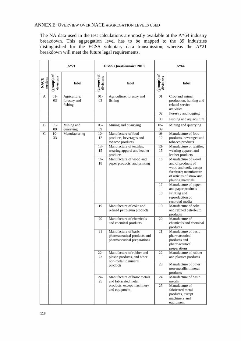
118
ANNEX E: OVERVIEW OVER NACE AGGREGATION LEVELS USED
The NA data used in the test calculations are mostly available at the A*64 industry
breakdown. This aggregation level has to be mapped to the 39 industries
distinguished for the EGSS voluntary data transmission, whereas the A*21
breakdown will meet the future legal requirements.
A*21 EGSS Questionnaire 2013 A*64
NA
CE
sect
ion
s
(gro
up
s) o
f
div
isio
ns
label
(gro
up
s) o
f
div
isio
ns
label
(gro
up
s) o
f
div
isio
ns
label
A 01-
03
Agriculture,
forestry and
fishing
01-
03
Agriculture, forestry and
fishing
01 Crop and animal
production, hunting and
related service
activities
02 Forestry and logging
03 Fishing and aquaculture
B 05-
09
Mining and
quarrying
05-
09
Mining and quarrying 05-
09
Mining and quarrying
C 10-
33
Manufacturing 10-
12
Manufacture of food
products, beverages and
tobacco products
10-
12
Manufacture of food
products, beverages and
tobacco products
13-
15
Manufacture of textiles,
wearing apparel and leather
products
13-
15
Manufacture of textiles,
wearing apparel and
leather products
16-
18
Manufacture of wood and
paper products, and printing
16 Manufacture of wood
and of products of
wood and cork, except
furniture; manufacture
of articles of straw and
plaiting materials
17 Manufacture of paper
and paper products
18 Printing and
reproduction of
recorded media
19 Manufacture of coke and
refined petroleum products
19 Manufacture of coke
and refined petroleum
products
20 Manufacture of chemicals
and chemical products
20 Manufacture of
chemicals and chemical
products
21 Manufacture of basic
pharmaceutical products and
pharmaceutical preparations
21 Manufacture of basic
pharmaceutical
products and
pharmaceutical
preparations
22-
23
Manufacture of rubber and
plastic products, and other
non-metallic mineral
products
22 Manufacture of rubber
and plastics products
23 Manufacture of other
non-metallic mineral
products
24-
25
Manufacture of basic metals
and fabricated metal
products, except machinery
and equipment
24 Manufacture of basic
metals
25 Manufacture of
fabricated metal
products, except
machinery and
equipment

119
A*21 EGSS Questionnaire 2013 A*64
26 Manufacture of computer,
electronic and optical
products
26 Manufacture of
computer, electronic
and optical products
27 Manufacture of electrical
equipment
27 Manufacture of
electrical equipment
28 Manufacture of machinery
and equipment n.e.c.
28 Manufacture of
machinery and
equipment n.e.c.
29-
30
Manufacture of transport
equipment
29 Manufacture of motor
vehicles, trailers and
semi-trailers
30 Manufacture of other
transport equipment
31-
33
Manufacture of furniture;
other manufacturing; repair
and installation of machinery
and equipment
31-
32
Manufacture of
furniture; other
manufacturing
33 Repair and installation
of machinery and
equipment
D 35 Electricity, gas,
steam and air
conditioning
supply
35 Electricity, gas, steam and air
conditioning supply
35 Electricity, gas, steam
and air conditioning
supply
E 36-
39
Water supply;
sewerage, waste
management and
remediation
activities
36 Water collection, treatment
and supply
36 Water collection,
treatment and supply
37 Sewerage 37-
39
Sewerage; waste
collection, treatment
and disposal activities;
materials recovery;
remediation activities
and other waste
management services
38 Waste collection, treatment
and disposal activities;
materials recovery
39 Remediation activities and
other waste management
services
F 41-
43
Construction 41-
43
Construction 41-
43
Construction
G 45-
47
Wholesale and
retail trade; repair
of motor vehicles
and motorcycles
45-
47
Wholesale and retail trade;
repair of motor vehicles and
motorcycles
45 Wholesale and retail
trade and repair of
motor vehicles and
motorcycles
46 Wholesale trade, except
of motor vehicles and
motorcycles
47 Retail trade, except of
motor vehicles and
motorcycles
H 49-
53
Transportation and
storage
49-
53
Transportation and storage 49 Land transport and
transport via pipelines
50 Water transport
51 Air transport
52 Warehousing and
support activities for
transportation
53 Postal and courier
activities
I 55-
56
Accommodation
and food service
activities
55-
56
Accommodation and food
service activities
55-
56
Accommodation; food
and beverage service
activities
J 58-
63
Information and
communication
58-
63
Information and
communication
58 Publishing activities
59-
60
Motion picture, video
and television
programme production,
sound recording and
music publishing

120
A*21 EGSS Questionnaire 2013 A*64
activities; programming
and broadcasting
activities
61 Telecommunications
62-
63
Computer
programming,
consultancy and related
activities; information
service activities
K 64-
66
Financial and
insurance activities
64-
66
Financial and insurance
activities
64 Financial service
activities, except
insurance and pension
funding
65 Insurance, reinsurance
and pension funding,
except compulsory
social security
66 Activities auxiliary to
financial services and
insurance activities
L 68 Real estate
activities
68 Real estate activities 68 Real estate activities
of which: imputed rents
of owner-occupied
dwellings
M 69-
75
Professional,
scientific and
technical activities
69-
70
Legal and accounting
activities; activities of head
offices; management
consultancy activities
69-
70
Legal and accounting
activities; activities of
head offices;
management
consultancy activities
71 Architecture and engineering
activities; technical testing
and analysis
71 Architecture and
engineering activities;
technical testing and
analysis
72 Scientific research and
development
72 Scientific research and
development
73-
75
Advertising and market
research; other professional,
scientific and technical
activities; veterinary
activities
73 Advertising and market
research
74-
75
Other professional,
scientific and technical
activities; veterinary
activities
N 77-
82
Administrative and
support service
activities
77-
82
Administrative and support
service activities
77 Rental and leasing
activities
78 Employment activities
79 Travel agency, tour
operator reservation
service and related
activities
80-
82
Security and
investigation activities;
services to buildings
and landscape
activities; office
administrative, office
support and other
business support
O 84 Public
administration and
defence;
compulsory social
security
84 Public administration and
defence; compulsory social
security
84 Public administration
and defence;
compulsory social
security

121
A*21 EGSS Questionnaire 2013 A*64
P 85 Education 85 Education 85 Education
Q 86-
88
Human health and
social work
activities
86-
88
Human health and social
work activities
86 Human health activities
87-
88
Social work activities
R 90-
93
Arts, entertainment
and recreation
90-
93
Arts, entertainment and
recreation
90-
92
Creative, arts and
entertainment activities;
libraries, archives,
museums and other
cultural activities;
gambling and betting
activities
93 Sports activities and
amusement and
recreation activities
S 94-
96
Other service
activities
94-
96
Other service activities 94 Activities of
membership
organisations
95 Repair of computers
and personal and
household goods
96 Other personal service
activities
T 97-
98
Activities of
households as
employers;
undifferentiated
goods- and
services-producing
activities of
households for
own use
97-
98
Activities of households as
employers; undifferentiated
goods- and services-
producing activities of
households for own use
97-
98
Activities of
households as
employers of domestic
personnel and
undifferentiated goods
and services production
of households for own
use
U 99 Activities of extra-
territorial
organisations and
bodies
99 Activities of extra-territorial
organisations and bodies
99 Activities of
extraterritorial
organizations and
bodies

122
ANNEX F: DATA SOURCES USED IN THE TEST CALCULATIONS
a) Eurostat data collections
Collection name Acronym
National Accounts aggregates by industry (up to NACE A*64) nama_10_a64
Annual National Accounts by 64 branches at current prices nama_nace64_c
National Accounts employment data by industry (up to NACE A*64) nama_10_a64_e
National Accounts by 64 branches - employment data nama_nace64_e
Supply table - current prices (NACE Rev. 2) naio_cp15_r2
Use table - current prices (NACE Rev. 2) naio_cp16_r2
Gross capital formation by industry (up to NACE A*64) nama_10_a64_p5
Gross capital formation by 64 branches - at current prices nama_pi64_c
Cross-classification of gross fixed capital formation by industry and by non-
financial fixed asset - current prices
nama_pi22_21_c
Average number of usual weekly hours of work in main job, by sex,
professional status, full-time/part-time and economic activity (from 2008
onwards, NACE Rev. 2) - hours
lfsa_ewhun2
Average number of usual weekly hours of work in main job, by sex,
professional status, full-time/part-time and economic activity (1983-2008,
NACE Rev. 1.1) - hours
lfsa_ewhuna
Full-time and part-time employment by sex and economic activity (from 2008
onwards, NACE Rev. 2) - 1 000
lfsa_epgan2
Full-time and part-time employment by sex and economic activity (1983-
2008, NACE Rev. 1.1) (1 000)
lfsa_epgana
Euro/ECU exchange rates – annual data ert_bil_eur_a
Environmental protection expenditure in Europe - detailed data (NACE Rev.
2)
env_ac_exp1r2
Certified organic crop area food_in_porg1
Land use - 1 000 ha - annual data apro_cpp_luse
Annual detailed enterprise statistics on electricity, gas and water supply
(NACE Rev. 1.1., E)
sbs_na_2a_el
Annual detailed enterprise statistics for industry (NACE Rev. 2, B-E) sbs_na_ind_r2
Supply, transformation, consumption - gas - annual data nrg_103a
Supply, transformation, consumption - electricity - annual data nrg_105a
Supply, transformation, consumption – renewable energies - annual data nrg_107a
Infrastructure – biofuel production capacities - annual data nrg_114a
Gas - domestic consumers - bi-annual prices - new methodology from
2007 onwards
nrg_pc_202
Electricity prices components for domestic consumers, from 2007 onwards -
annual data
nrg_pc_204_c
Electricity prices components for industrial consumers, from 2007 onwards -
annual data
nrg_pc_205_c
Infrastructure - electricity - annual data nrg_113a
Statistics on the production of manufactured goods prom
Traditional international trade database access) ComEx
International trade of EU, the euro area and the Member States by SITC
product group
ext_lt_intertrd
Balance of payments by country bop_q_c

123
b) Other sources
Bundesministerium für Ernährung, Landwirtschaft und Verbraucherschutz. (2012). Die
wirtschaftliche Lage der landwirtschaftlichen Betriebe - Buchführungsergebnisse der Testbetriebe,
Wirtschaftsjahr 2011/12.
Bundesministerium für Umwelt, Naturschutz und Reaktorsicherheit:
- (various editions). Erneuerbare Energien in Zahlen - Nationale und internationale Entwicklung.
- (2013). Investitionen für ein klimafreundliches Deutschland - Eine Studie im Auftrag des
Bundesministerium für Umwelt, Naturschutz und Reaktorsicherheit.
- (various editions). Erneuerbare Energien in Zahlen - Internet-Update ausgewählter Daten.
Bundesnetzagentur; Bundeskartellamt. (2012). Monitoringbericht 2012. Retrieved 06 19, 2012
Bundesverband der deutschen Bioethanolwirtschaft e.V. (2013). Umrechnungsformeln für
Biokraftstoffe.
Deutsche Energieagentur (dena). (2010). dena-Sanierungsstudie. Teil 1: Wirtschaftlichkeit
energetischer Modernisierung im Mietwohnungsbestand.
FAO, OECD (2013 and earlier issues): Agricultural Outlook
International Energy Agency; Nuclear Energy Agency. (2010). Projected Costs of Generating
Electricity.
KFW Bankengruppe. (2014 and earlier issues). Monitoring der KfW-Programme „Energieeffizient
Sanieren“ und „Energieeffizient Bauen“
Prognos AG. (2010). Investitionen durch den Ausbau erneuerbarer Energien in Deutschland.
Thünen-Institut. (2013). Analyse der wirtschaftlichen Lage ökologisch wirtschaftender Betriebe.
Verordnung über die Honorare für Architekten- und Ingenieurleistungen (HOIA): Honorartafel zu §
16 Abs. 1 HOAI (Objektplanung Gebäude)

124
BIBLIOGRAPHY
Agence de l'Environnement et de la Maîtrise de l'Energie. (2013). Batiment, Edition
2013.
Baud, S. (2012). Umweltorientierte Produktion und Dienstleistung (EGSS) 2011 -
Umsatz und Beschäftigte in der Umweltwirtschaft.
Blazejczak, J., & Edler, D. (2012). Methods for estimation of gross employment
effects of environmental protection. Berlin: German Institute for Economic
Research (DIW Berlin).
Bundesministerium für Ernährung, Landwirtschaft und Verbraucherschutz. (2012a).
Die wirtschaftliche Lage der landwirtschaftlichen Betriebe -
Buchführungsergebnisse der Testbetriebe, Wirtschaftsjahr 2011/12.
Bundesministerium für Ernährung, Landwirtschaft und Verbraucherschutz. (2012b).
Kleinere Ernte, höhere Erlöse - Biolandwirte blicken auf ein erfolgreiches
Jahr 2010 zurück, Press release no. 46 of 13.02.12.
Bundesministerium für Umwelt, Naturschutz und Reaktorsicherheit. (2011).
Erneuerbare Energien 2010.
Bundesministerium für Umwelt, Naturschutz und Reaktorsicherheit. (2012).
Erneuerbare Energien in Zahlen - Internet-Update ausgewählter Daten.
Bundesministerium für Umwelt, Naturschutz und Reaktorsicherheit. (2013a).
Erneuerbare Energien in Zahlen - Nationale und internationale Entwicklung.
Bundesministerium für Umwelt, Naturschutz und Reaktorsicherheit. (2013b).
Investitionen für ein klimafreundliches Deutschland - Eine Studie im Auftrag
des Bundesministerium für Umwelt, Naturschutz und Reaktorsicherheit.
Bundesnetzagentur; Bundeskartellamt. (2012). Monitoringbericht 2012.
Bundesverband der deutschen Bioethanolwirtschaft e.V. (2013).
Umrechnungsformeln für Biokraftstoffe.
Bureau of Labor Statistics (BLS). (2013a). Employment in Green Goods and
Servcies – 2011.
Bureau of Labor Statistics (BLS). (2013b). Extended Technical Note.
Constantino, S., Fritzsche, J., Obst, C., Schenau, S., Steinbach, N., & Steurer, A.
(2013). State of debate note on the Environmental Goods and Services Sector
(EGSS). London.
DESTATIS. (2014). Produzierendes Gewerbe - Beschäftigung und Umsatz der
Betriebe des Verarbeitenden Gewerbes sowie des Bergbaus und der
Gewinnung von Steinen und Erden, Fachserie, 4 Reihe 4.1.1.
Deutsche Energieagentur (dena). (2010). dena-Sanierungsstudie. Teil 1:
Wirtschaftlichkeit energetischer Modernisierung im Mietwohnungsbestand.

125
Eckermann, F. (2012). Beschäftigung im Umweltschutz.
Economics and Statistics Administration. (2010a). Measuring the Green Economy.
Economics and Statistics Administration. (2010b). Measuring the Green Economy -
Appendix 2: Methodology for Estimating Shipments/Receipts and
Employment for Green Products and Services.
ECORYS. (2009). Study on the Competitiveness of the EU eco-industry.
ECORYS. (2012). The number of Jobs dependent on the Environment and Resource
Efficiency improvements.
ECOTEC. (1999). Analysis of the EU Eco-Industries, their Employment and Export
Potential.
Edler, D., & Blazejczak, J. (2012). Beschäftigungswirkungen des Umweltschutzes in
Deutschland im Jahr 2008.
Edler, D., Blazejczak, J., Wackerbauer, J., Rave, T., Legler, H., & Schasse, U.
(2009). Beschäftigungswirkungen des Umweltschutzes in Deutschland im
Jahr 2006.
Ernst & Young Environment and Sustainability Services. (2006). Eco-industries, its
size, employment, perspectives, and barriers to growth in an enlarged EU.
European Commission. (2012). Towards a job-rich recovery.
European Commission. (2013). Market observatory & Statistics.
European Commission, FAO, IMF, OECD, UN, World Bank. (2012). System of
Envrionmental-Economic Accounting: Central Framework, White cover
publication, pre-edited text subject to official editing.
European Commission, IMF, OECD, UN, World Bank. (2008). System of National
Accounts 2008.
Eurostat. (1996). European system of accounts (ESA 1995). Luxembourg: Office for
Official Publications of the European Communities.
Eurostat. (2000). Manual on the Economic Accounts for Agriculture and Forestry
(Rev. 1.1.).
Eurostat. (2002). SERIEE - European System for the collection of economic
information on the environment — 1994 Version.
Eurostat. (2005a). Environmental expenditure statistics: Industry data collection
handbook.
Eurostat. (2005b). Environmental Protection Expenditure and Revenue Joint
Questionnaire/SERIEE Environmental Protection Expenditure Account,
Conversion Guidelines.

126
Eurostat. (2007). Environmental expenditure statistics 2007 edition: General
Government and Specialised Producers data collection handbook.
Eurostat. (2008). NACE Rev. 2 - Statistical classification of economic activities in the
European Community.
Eurostat. (2009). The environmental goods and services sector - A data collection
handbook.
Eurostat. (2011). Manual on sources and methods for the compilation of COFOG
Statistics.
Eurostat. (2012a). Minutes of the 1-2 March 2012 meeting of the subgroup on
environmental activity and expenditure classifications, , Subgroup of the Task
Forces on environmental transfers and on RUMEA. Retrieved 10 29, 2013,
from CIRCABC:
Eurostat. (2012b). Overview of existing classifications with relevance for the
subgroup, Subgroup of the Task Forces on environmental transfers and on
RUMEA.
Eurostat. (2012c). Proposal for new modules for inclusion in Regulation 691/2011:
Environmental goods and services sector, Joint meeting of the Working
Groups on environmental accounts and environmental expenditure statistics.
Eurostat. (2012d). Regulation on European Environmental Economic Accounts: New
modules, Directors' Meeting on Environmental Statistics and Accounts, 20
November 2012.
Eurostat. (2013a). Environmental expenditure variables in the SBS Regulation –
Results of the work of the electronic discussion group (EDG) on the SBS
environmental variables and next steps. Luxembourg: Eurostat.
Eurostat. (2013b). Further integrating the monetary environmental accounts.
Eurostat. (2013c). The resource management expenditure account (ReMEA),
Working Group Environmental Expenditure Statistics, Meeting of 20 - 21
March 2013 Doc. ENV/EXP/WG/4 (2013).
Eurostat. (2013d). Draft minutes of the meeting of the task force on the resource
management expenditure account (ReMEA) of 16-17 October 2013, Version
of 7 November 2013. Luxembourg.
Eurostat. (2013e). European System of Accounts (ESA 2010).
Eurostat. (2013f). International trade data, Reference Metadata in Euro SDMX
Metadata Structure (ESMS).
Eurostat. (2013g). Electricity Prices - Price Systems 2012.
Eurostat. (2014). Revision of the 2009 EGSS Handbook, Doc.
ENV/EXP/WG/3.3(2014).
127
FAO, OECD. (2011). Agricultural Outlook 2012-2021.
Fondation d’entreprise Alcen pour la Connaissance des Énergies. (2013).
Tarification de l’électricité.
Gehrke, B., & Schasse, U. (2013). Umweltschutzgüter - wie abgrenzen? Methodik
und Liste der Umweltschutzgüter 2013.
GHK Consulting. (2007). Links between the environment, economy and jobs.
Greffet, P., Mauroux, A., Ralle, P., & Randriambololona, C. (2012). Définir et
quantifier l’économie verte.
Institut für Arbeitsmarkt- und Berufsforschung. (2013). Aktuelle Daten und
Indikatoren zur Arbeitsmarktentwicklung in Ost- und Westdeutschland,
Durchschnittliche Arbeitszeit und ihre Komponenten (Stand: 03.04.2013).
International Energy Agency; Nuclear Energy Agency. (2010). Projected Costs of
Generating Electricity.
International Labour Organisation (ILO). (2013). Methodologies for assessing green
jobs. Policy brief, February 2013.
KFW Bankengruppe. (2011). Impact on public budgets of KFW promotional
programmes in the field of "energy-efffcient building and rehabilitation".
KFW Bankengruppe. (2013). Impact on public budgets of the KFW promotional
programmes in the field of "energy-efffcient construction", "energy-effcient
refurbishment" and "energy-effcient infrastructure" in 2011.
Kleine, S. (2012). Die umweltökonomischen Statistiken bis 2010.
Naturschutzbund Deutschland (NABU) e.V. (2011). Anforderungen an einen
Sanierungsfahrplan - Auf dem Weg zu einem klimafreundlichen
Gebäudebestand bis 2050.
OECD, Eurostat. (1999). The Environmental Goods & Servcies Industry - Manual
for Data Collection and Anlaysis.
OECD, IEA, Eurostat. (2004). Energy Statistics Manual.
Offermann, F., Sanders, J., & Nieberg, H. (n.d.). Method for selecting comparable
organic and conventional farms.
Official Journal of the European Union. (2013). REG. (EU) No 549/2013 OF THE
EUROPEAN PARLIAMENT AND OF THE COUNCIL of 21 May 2013 on the
European system of national and regional accounts in the European Union.
Prognos AG. (2010). Investitionen durch den Ausbau erneuerbarer Energien in
Deutschland.

128
Rørmose Jensen, P., & Månsson, H. (2012). The Environmental Goods and Service
Sector in Denmark. A Pilot Study. Report on Eurostat grant no.
50904.2011.005-2011.291. Copenhagen: Statistics Denmark.
Statistik Austria. (2012). Standard-Dokumentation Metainformationen (Definitionen,
Erläuterungen, Methoden, Qualität) zur Umweltorientierten Produktion und
Dienstleistung (EGSS).
Statistisches Bundesamt (DESTATIS). (2010). Erhebung der laufenden
Aufwendungen für den Umweltschutz.
Steenblik, R., & Geloso Grosso, M. (2011). Trade in Services Related to Climate
Change - an explanatory analysis, OECD Trade and Environment Working
Papers 2011/03.
Thünen-Institut. (2013). Analyse der wirtschaftlichen Lage ökologisch
wirtschaftender Betriebe.
Umweltbundesamt. (2008). Beschäftigung im Umweltschutz.
van Rossum, M. (2012). Economic indicators for the Dutch Environmental Goods
and Services Sector - Time series data for 1995-2009.
Voram, J., & van Rossum, M. (2013). Economic Radar of the Sustainable Energy
Sector in the Netherlands, 2008–2011.
Workforce Information Council, Green Jobs Study Group. (2009). Measurement and
analysis of employment in the green economy.