a polynomial-time algorithm for global value numbering · pdf filethere are programs for which...

Science of Computer Programming 64 (2007) 97–114www.elsevier.com/locate/scico

A polynomial-time algorithm for global value numbering

Sumit Gulwania,∗, George C. Neculab

a Microsoft Corporation, One Microsoft Way, Redmond, WA 98052, USAb Department of Computer Science, UC-Berkeley, Berkeley, CA 94720, USA

Received 31 January 2005; received in revised form 15 October 2005; accepted 15 March 2006Available online 9 October 2006

Abstract

We describe a polynomial-time algorithm for global value numbering, which is the problem of discovering equivalences amongprogram sub-expressions. We treat all conditionals as non-deterministic and all program operators as uninterpreted. We show thatthere are programs for which the set of all equivalences contains terms whose value graph representation requires exponentialsize. Our algorithm discovers all equivalences among terms of size at most s in time that grows linearly with s. For global valuenumbering, it suffices to choose s to be the size of the program. Earlier deterministic algorithms for the same problem are eitherincomplete or take exponential time. We provide a detailed analytical comparison of some of these algorithms.c© 2006 Elsevier B.V. All rights reserved.

Keywords: Global value numbering; Uninterpreted functions; Abstract interpretation; Herbrand equivalences

1. Introduction

Detecting equivalence of program sub-expressions has a variety of applications. Compilers use this informationto perform several important optimizations like constant and copy propagation [17], common sub-expressionelimination, invariant code motion [2,14], induction variable elimination, branch elimination, branch fusion, and loopjamming [9]. Program verification tools use these equivalences to discover loop invariants, and to verify programassertions. This information is also important for discovering equivalent computations in different programs; thisis useful for plagiarism detection tools and translation validation tools [13,12], which compare a program with anoptimized version in order to check the correctness of the optimizer.

Checking equivalence of program expressions is an undecidable problem, even when all conditionals are treated asnon-deterministic. Most tools, including compilers, attempt to only discover equivalences between expressions thatare computed using the same operator applied to equivalent operands. This form of equivalence, where the operatorsare treated as uninterpreted functions, is also called Herbrand equivalence [16]. The process of discovering such arestricted class of equivalences is often referred to as value numbering. Performing value numbering in basic blocksis an easy problem; the challenge is in doing it globally for a procedure body.

∗ Corresponding author.E-mail addresses: [email protected] (S. Gulwani), [email protected] (G.C. Necula).URLs: http://research.microsoft.com/∼sumitg (S. Gulwani), http://www.cs.berkeley.edu/∼necula (G.C. Necula).

0167-6423/$ - see front matter c© 2006 Elsevier B.V. All rights reserved.doi:10.1016/j.scico.2006.03.005

http://www.elsevier.com/locate/scico

mailto:[email protected]

mailto:[email protected]

http://research.microsoft.com/~sumitg





http://www.cs.berkeley.edu/~necula






http://dx.doi.org/10.1016/j.scico.2006.03.005

98 S. Gulwani, G.C. Necula / Science of Computer Programming 64 (2007) 97–114

Existing deterministic algorithms for global value numbering are either too expensive or imprecise. The precisealgorithms are based on an early algorithm by Kildall [8], which discovers equivalences by performing an abstractinterpretation [3] over the lattice of Herbrand equivalences. Kildall’s algorithm discovers all Herbrand equivalencesin a function body, but has exponential cost [16]. On the other extreme, there are several polynomial-time algorithmsthat are complete for basic blocks, but are imprecise in the presence of joins and loops in a program. The popularpartition refinement algorithm proposed by Alpern, Wegman, and Zadeck (AWZ) [1] is particularly efficient, butat the price of being significantly less precise than Kildall’s algorithm. The novel idea in the AWZ algorithm is torepresent the values of variables after a join using a fresh selection function φi , similar to the functions used inthe static single assignment form [4], and to treat the φi functions as additional uninterpreted functions. The AWZalgorithm is incomplete because it treats φ functions as uninterpreted. In an attempt to remedy this problem, Ruthing,Knoop and Steffen have proposed a polynomial-time algorithm (RKS) [16] that alternately applies the AWZ algorithmand some rewrite rules for normalization of terms involving φ functions, until the congruence classes reach a fixedpoint. Their algorithm discovers more equivalences than the AWZ algorithm, but remains incomplete. The AWZand the RKS algorithms both use a data structure called the value graph [9], which encodes the abstract syntax ofprogram sub-expressions, and represents equivalences by merging nodes that have been discovered to be referring toequivalent expressions. We discuss these algorithms in more detail in Section 5. Recently, Gargi has also proposed aset of balanced algorithms that are efficient, but they too are incomplete [5].

Our algorithm is based on two novel observations. First, it is important to make a distinction between “discoveringall Herbrand equivalences” vs. “discovering Herbrand equivalences among program sub-expressions”. The formerinvolves discovering Herbrand equivalences among all terms that can be constructed using program variables anduninterpreted functions in the program. The latter refers to only those terms that occur syntactically in the program.Finding all Herbrand equivalences is attractive not only for answering questions about non-program terms, but italso allows forward dataflow or abstract interpretation based algorithms (e.g. Kildall’s algorithm) to discover allequivalences among program terms. This is because discovery of an equivalence between program terms at someprogram point may require detecting equivalences among non-program terms at a preceding program point. Thisdistinction is important, because we show (in Section 4) that there is a family of acyclic programs for which the setof all Herbrand equivalences requires an exponential sized (in the size of the program) value graph representation. Onthe other hand, we also show that Herbrand equivalences among program sub-expressions can always be representedusing a linear sized value graph. This implies that no algorithm that uses value graphs to represent equivalences candiscover all Herbrand equivalences and have polynomial-time complexity at the same time. This observation explainswhy existing polynomial-time algorithms for value numbering are incomplete, even for acyclic programs. One ofthe reasons why Kildall’s algorithm is exponential is that it discovers all Herbrand equivalences at each programpoint.

The above observation not only sheds light on the incompleteness or exponential complexity of the existingalgorithms, but also motivates the design of our algorithm. Our algorithm takes a parameter s and discovers allHerbrand equivalences, among terms of size at most s in time, and grows linearly with s. For the purpose of globalvalue numbering, it is sufficient to set the parameter s to N , where N is the size of the program, since the size of anyprogram expression is at most N .

The second observation is that the lattice of sets of Herbrand equivalences that can arise at any program pointin our abstracted program model (which only allows non-deterministic conditionals)has finite height k, where k isthe number of program variables. We prove this result in Section 3.6. Therefore, an optimistic-style algorithm thatperforms an abstract interpretation over the lattice of Herbrand equivalences, will be able to handle cyclic programsas precisely as it can handle acyclic programs, and will terminate in at most k iterations. Without this observation, onecan ensure the termination of the algorithm in the presence of loops by adding a degree of pessimism. This leads toincompleteness in the presence of loops, as is the case with the RKS algorithm [16]. Instead, our algorithm is basedon an abstract interpretation, similar to Kildall’s algorithm, while using a more sophisticated join operation. Note thateven though the lattice of Herbrand equivalences has small height, representing the lattice elements and performinglattice operations on them can take exponential time and space, as pointed out in the first observation above. Weavoid this problem by maintaining a bounded size approximation of lattice elementsthat is sufficient to discover allHerbrand equivalences of bounded size. We continue with a description of the expression language on which thealgorithm operates (in Section 2), followed by a description of the algorithm itself in Section 3.

S. Gulwani, G.C. Necula / Science of Computer Programming 64 (2007) 97–114 99

Fig. 1. Flowchart nodes.

2. Language of program expressions

We consider a language in which the expressions occurring in assignments belong to the following simple languageof uninterpreted function terms (here x is one of the variables, and c is one of the constants):

e ::= x | c | F(e1, e2).

For any expression e, we use the notation Variables(e) to denote the variables that occur in expression e. We usesize(e) to denote the number of occurrences of function symbols in expression e (when expressed as a value graph).For simplicity, we consider only one binary uninterpreted function F . Our results can be extended easily to languageswith any finite number of uninterpreted functions of any constant arity. Alternatively, we can model any uninterpretedfunction Fa of any constant arity a using the given binary uninterpreted function F by employing the followingclosure trick:

Fa(e1, . . . , ea) = F(e1, e′

2), where e′

i =

{F(ei , e′

i+1) for 2 ≤ i ≤ a − 1

F(ea, xFa ) for i = a.

Here xFa is a fresh variable (which can be regarded as a new input variable) associated with the uninterpreted functionFa . If we regard a to be a constant, then this modeling does not alter the quantities on which the computationalcomplexity of the algorithm depends (except by a constant factor).

3. The global value numbering algorithm

Our algorithm discovers the set of Herbrand equivalences at any program point by performing an abstractinterpretation over the lattice of Herbrand equivalences. We pointed out in the introduction, and we argue furtherin Section 4, that we cannot hope to have a complete and polynomial-time algorithm that discovers all Herbrandequivalences implied by a program (using the standard value graph based representations) because their representationis a worst-case exponential in the size of the program. Thus, our algorithm takes a parameter s (which is a positiveinteger) and discovers all equivalences of the form e1 = e2, where size(e1) ≤ s and size(e2) ≤ s. The algorithm usesa data structure called Strong Equivalence DAG (described in Section 3.1) to represent the set of equivalences at anyprogram point. It updates the data structure across the flowchart nodes shown in Fig. 1 using the transfer functionsdescribed in Section 3.2 through Section 3.5. In the presence of loops, it goes around loops until a fixed point isreached, as described in Section 3.6.

3.1. Notation and data structure (SED)

Let T be the set of all program variables, k the total number of program variables, and N the size of the program,measured in terms of the number of occurrences of function symbol F in the program.

The algorithm represents the set of equivalences at any program point by a data structure that we call StrongEquivalence DAG (SED). An SED is similar to a value graph. It is a labeled, directed acyclic graph, whose nodes η

can be represented by tuples 〈V, t〉, where V is a (possibly empty) set of program variables labeling the node, andt represents the type of node. The type t is either ⊥ or c, indicating that the node has no successors, or F(η1, η2),indicating that the node has two ordered successors η1 and η2.

In any SED G, for every variable x , there is exactly one node 〈V, t〉, denoted by NodeG(x), such that x ∈ V . Forevery type t that is not ⊥, there is at most one node of that type. We use the notation NodeG(c) to refer to the nodewith type c. For any SED node η, we use the notation Vars(η) to denote the set of variables labeling node η, and


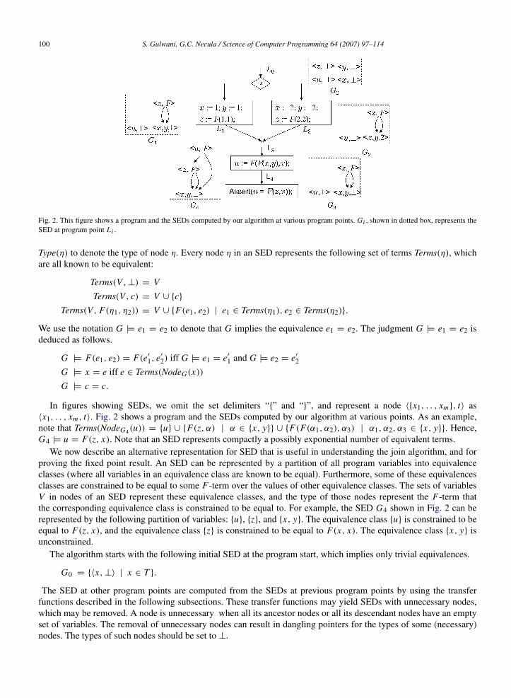
Fig. 2. This figure shows a program and the SEDs computed by our algorithm at various program points. Gi , shown in dotted box, represents theSED at program point L i .

Type(η) to denote the type of node η. Every node η in an SED represents the following set of terms Terms(η), whichare all known to be equivalent:

Terms(V, ⊥) = V

Terms(V, c) = V ∪ {c}

Terms(V, F(η1, η2)) = V ∪ {F(e1, e2) | e1 ∈ Terms(η1), e2 ∈ Terms(η2)}.

We use the notation G |= e1 = e2 to denote that G implies the equivalence e1 = e2. The judgment G |= e1 = e2 isdeduced as follows.

G |= F(e1, e2) = F(e′

1, e′

2) iff G |= e1 = e′

1 and G |= e2 = e′

2

G |= x = e iff e ∈ Terms(NodeG(x))

G |= c = c.

In figures showing SEDs, we omit the set delimiters “{” and “}”, and represent a node 〈{x1, . . , xm}, t〉 as〈x1, . . , xm, t〉. Fig. 2 shows a program and the SEDs computed by our algorithm at various points. As an example,note that Terms(NodeG4(u)) = {u} ∪ {F(z, α) | α ∈ {x, y}} ∪ {F(F(α1, α2), α3) | α1, α2, α3 ∈ {x, y}}. Hence,G4 |= u = F(z, x). Note that an SED represents compactly a possibly exponential number of equivalent terms.

We now describe an alternative representation for SED that is useful in understanding the join algorithm, and forproving the fixed point result. An SED can be represented by a partition of all program variables into equivalenceclasses (where all variables in an equivalence class are known to be equal). Furthermore, some of these equivalencesclasses are constrained to be equal to some F-term over the values of other equivalence classes. The sets of variablesV in nodes of an SED represent these equivalence classes, and the type of those nodes represent the F-term thatthe corresponding equivalence class is constrained to be equal to. For example, the SED G4 shown in Fig. 2 can berepresented by the following partition of variables: {u}, {z}, and {x, y}. The equivalence class {u} is constrained to beequal to F(z, x), and the equivalence class {z} is constrained to be equal to F(x, x). The equivalence class {x, y} isunconstrained.

The algorithm starts with the following initial SED at the program start, which implies only trivial equivalences.

G0 = {〈x, ⊥〉 | x ∈ T }.

The SED at other program points are computed from the SEDs at previous program points by using the transferfunctions described in the following subsections. These transfer functions may yield SEDs with unnecessary nodes,which may be removed. A node is unnecessary when all its ancestor nodes or all its descendant nodes have an emptyset of variables. The removal of unnecessary nodes can result in dangling pointers for the types of some (necessary)nodes. The types of such nodes should be set to ⊥.


3.2. Assignment node

See Fig. 1(a). Let G be an SED that represents the Herbrand equivalences before an assignment node x := e.The SED that represents the Herbrand equivalences after the assignment node can be obtained by using the followingAssignment function. SED G4 in Fig. 2 shows an example of the Assignment function.

Assignment(G ′, x := e) =1 G := G ′;2 let 〈V1, t1〉 = GetNode(G, e) in3 let 〈V2, t2〉 = NodeG(x) in4 ReplaceVars(G, 〈V1, t1〉, V1 ∪ {x});5 ReplaceVars(G, 〈V2, t2〉, V2 − {x});6 return G;

GetNode(G, e) =1 match e with2 y: return NodeG(y);3 F(e1, e2): let η1 = GetNode(G, e1) and η2 = GetNode(G, e2) in4 if 〈V, F(η1, η2)〉 ∈ G for some V, return 〈V, F(η1, η2)〉;5 else G := G ∪ 〈∅, F(η1, η2)〉; return 〈∅, F(η1, η2)〉;

GetNode(G, e) returns a node η such that e ∈ Terms(η) (and in the process possibly extends G) in O(size(e)) time.ReplaceVars(G, η, V ) replaces the set of variables in node η by V (in place) in SED G. Lines 4 and 5 in Assignmentfunction move variable x to the node GetNode(G, e) to reflect the equivalence x = e. Hence, the following lemmaholds.

Lemma 1 (Soundness and Completeness of Assignment). Let G = Assignment(G ′, x := e). Let e1 and e2 be twoexpressions. Let e′

1 = e1[e�x ] and e′

2 = e2[e�x ]. Then, G |= e1 = e2 iff G ′

|= e′

1 = e′

2.

3.3. Non-deterministic assignment node

See Fig. 1(b). If the SED G ′ before a non-deterministic assignment node is ⊥, then the SED G after the non-deterministic assignment node is also ⊥. Otherwise, the SED G after a non-deterministic assignment node x :=? isobtained from SED G ′ using the following function, which removes variable x from NodeG ′(x), and creates a newnode 〈{x}, >〉.

Non-det-Assignment(G ′, x :=?) =1 G := G ′;2 let 〈V, t〉 = NodeG(x) in3 ReplaceVars(G, 〈V, t〉, V − {x});4 G := G ∪ {〈{x}, >〉};5 return G;

The following lemma holds.

Lemma 2 (Soundness and Completeness of Non-det-Assignment). Let G = Non − det − Assignment(G ′, x :=

?). Let e1 and e2 be two expressions. Let e′

1 = e1[x ′

�x ] and e′

2 = e2[x ′

�x ] for some fresh variable x ′ that does notoccur in e1 and e2. Then, G |= e1 = e2 iff G ′

|= e′

1 = e′

2.

3.4. Non-deterministic conditional node

See Fig. 1(c). The SEDs G1 and G2 on the two branches of a non-deterministic conditional node are simply a copyof the SED G before the non-deterministic conditional node.


3.5. Join node

See Fig. 1(d). Let G1 and G2 be two SEDs. Let s′ be any positive integer. The following function Join returnsan SED G that represents all equivalences e1 = e2, such that both G1 and G2 imply e1 = e2 and both size(e1) andsize(e2) are at most s′. In order to discover all the equivalences among expressions of size at most s in the program,we need to choose s′

= s + N × k (for reasons explained later in Section 3.7). Fig. 2 shows an example of the Joinfunction.

For any SED G, let ≺G denote a partial ordering on the program variables such that x ≺G y if y depends on x , ormore precisely, if G |= y = F(e1, e2) such that x ∈ Variables(F(e1, e2)).

Join(G1,G2,s′) =1 for all nodes η1 ∈ G1 and η2 ∈ G2, memoize[η1, η2] := undefined;2 G := ∅;3 for each variable x ∈ T in the order ≺G1 do4 counter := s′;5 Intersect(NodeG1(x), NodeG2(x));6 return G;

Intersect(〈V1, t1〉,〈V2, t2〉) =1 let m = memoize(〈V1, t1〉, 〈V2, t2〉) in2 if m 6= undefined then return m;3 let t = if counter > 0 and t1 ≡ F(`1, r1) and t2 ≡ F(`2, r2) then4 counter := counter − 1;5 let ` = Intersect(`1,`2) in6 let r = Intersect(r1,r2) in7 if (` 6= 〈φ, ⊥〉) and (r 6= 〈φ, ⊥〉) then F(`, r) else ⊥

8 else if t1 = c and t2 = c for some c, then c9 else ⊥ in

10 let V = V1 ∩ V2 in11 if V 6= ∅ or t 6= ⊥ then G := G ∪ {〈V, t〉}12 memoize[〈V1, t1〉, 〈V2, t2〉] := 〈V, t〉;13 return 〈V, t〉

The Join function is similar to the finite automata intersection algorithm. It is easier to understand the Joinfunction by ignoring the use of the counter variable, which is introduced for efficiency reasons rather than correctness.If we ignore the use of counter variable, then Join(G1, G2, s′) returns an SED G such that G implies all equivalencesthat are implied by both G1 and G2. In that case however, the size of G as well as the computational complexity of theJoin function will be quadratic in the size of G1 and G2. Hence a join of n SEDs may result in an SED whose size isexponential in the size of the input SEDs. (This would be the case, for example, for the program shown in Fig. 5.)

The use of a counter variable produces a pruned version of G that maintains all equivalences of size at most s′ (asstated formally in Lemma 4). The pruned version of G represents the SED that can be obtained from G by removingconstraints of those equivalence classes represented by G (recall the alternative representation of SEDs as discussedin Section 3.1) that are of size greater than s′. Computing a pruned version of G as opposed to G itself is sufficient,since we are interested in computing equivalences of bounded size rather than all equivalences. The use of a countervariable thus ensures that the call to Intersect function in Join terminates in O(s′) time. Hence, the complexityof the Join function with use of a counter variable is O(s′

× k). An alternative would have been to compute G byrunning the Join function without the use of a counter variable, and then pruning G. This would, however have anincreased computational complexity of O(s′2).

The following proposition describes the property of Intersect function that is required to prove the correctnessof the Join function (Lemma 4).


Proposition 3. Let η1 = 〈V1, t1〉 and η2 = 〈V2, t2〉 be any nodes in SEDs G1 and G2 respectively. Let n = 〈V, t〉 =

Intersect(η1, η2). Suppose that n 6= 〈∅, ⊥〉; hence the function Intersect(η1, η2) adds the node n to G. Let α bethe value of the counter variable when Intersect(η1, η2) is first called. Then,

(P1) Terms(η) ⊆ Terms(η1) ∩ Terms(η2).(P2) Terms(η) ⊇ {e | e ∈ Terms(η1), e ∈ Terms(η2), size(e) ≤ α}.

The proof of Proposition 3 is by induction on the sum of height of nodes η1 and η2 in G1 and G2 respectively.We sketch a brief outline of the proof here; the detailed proof is given in Appendix A.1. Claim P1 follows fromthe observation that t = F(...) or c only if both t1 and t2 are F(...) or c respectively (lines 7 and 8), andV = V1 ∩ V2 (line 10). Claim P2 relies on bottom-up processing of one of the SEDs (line 3 in Join function),and memoization of calls to the Intersect function (line 12). Let e′ be one of the smallest expressions (in terms ofsi ze) such that e′

∈ Terms(η1) ∩ Terms(η2). If e′ is not a variable, then for any variable y ∈ Variables(e′), the callIntersect(NodeG1(y), NodeG2(y)) has already finished. The crucial observation now is that if size(e′) ≤ α, thenthe set of recursive calls to Intersect are in 1-1 correspondence with the nodes of expression e′, and e′

∈ Terms(η).

Lemma 4 (Soundness and Completeness of Join). Let G = Join(G1, G2, s). If G |= e1 = e2, then G1 |= e1 = e2and G2 |= e1 = e2. If G1 |= e1 = e2 and G2 |= e1 = e2 such that size(e1) ≤ s and size(e2) ≤ s, then G |= e1 = e2.

The proof of Lemma 4 follows from Proposition 3 and the definition of |=.

3.6. Fixed point computation

The algorithm goes around loops in a program until a fixed point is reached. The following theorem implies that thealgorithm needs to execute each flowchart node at most k times (assuming the standard worklist implementation [9]).

Theorem 1 (Fixed Point Theorem). Let G1, . . . , G` be the SEDs computed by the algorithm at some program pointinside a loop in successive iterations of that loop such that Gi+1 implies a strictly smaller subset of equivalences thanthose implied by Gi . Then, ` ≤ k + 1, where k is the number of program variables.

Proof. Consider the alternative representation of SEDs in terms of partitions of constrained or unconstrainedequivalence classes of the program variables (as discussed in Section 3.1). Now observe that Gi can be obtainedfrom Gi+1 only by constraining an unconstrained equivalence class or by merging an unconstrained equivalenceclass with another (constrained or unconstrained) equivalence class. Hence, the number of unconstrained equivalenceclasses in Gi is strictly smaller than in Gi+1. Since the number of unconstrained equivalence classes in G` can be atmost k, the result follows.

3.7. Correctness of the algorithm

The correctness of the algorithm follows from Theorems 2 and 3.

Theorem 2 (Soundness Theorem). Let G be the SED computed by the algorithm at some program point P after fixedpoint computation. If G |= e1 = e2, then e1 = e2 holds at program point P.

The proof of Theorem 2 follows directly from the soundness of the assignment operation (Lemma 1 in Section 3.2),non-det-assignment operation (Lemma 2 in Section 3.3) and the join operation (Lemma 4 in Section 3.5).

Theorem 3 (Completeness Theorem). Let e1 = e2 be an equivalence that holds at a program point P such thatsize(e1) ≤ s and size(e2) ≤ s. Let G be the SED computed by the algorithm at program point P after fixed pointcomputation. Then, G |= e1 = e2.

The proof of Theorem 3 follows from an invariant maintained by the algorithm at each program point. For thepurpose of describing this invariant, we hypothetically extend the algorithm to maintain a set S of paths at eachprogram point (representing the set of all paths analyzed by the algorithm), and a variable MaxSize (representing thesize of the largest expression computed by the program along any path in S) besides an SED. These are updated asshown in Fig. 3. The initial value of MaxSize is chosen to be 0. The initial set of paths is chosen to be the singletonset containing an empty path. The algorithm maintains the following invariant at each program point.


Fig. 3. Flowchart nodes.

Lemma 5. Let G be the SED, m be the value of variable MaxSize, and S be the set of paths computed by the algorithmat some program point P. Suppose e1 = e2 holds at program point P along all paths in S, size(e1) ≤ s′

− m andsize(e2) ≤ s′

− m. Then, G |= e1 = e2.

The proof of Lemma 5 is by induction on the number of operations performed by the algorithm, and is given inAppendix A.2.

Theorem 1 (the fixed point theorem) requires the algorithm to execute each node at most k times. This implies thatthe value of the variable MaxSize at any program point after the fixed point computation is at most N × k. Hence,choosing s′

= s + N × k enables the algorithm to discover equivalences among expressions of size s. The proof ofTheorem 3 now follows easily from Lemma 5.

3.8. Complexity analysis

Let j be the number of join points in the program. Let I be the maximum number of iterations of any loopperformed by the algorithm. (It follows from Theorem 1 that I is upper bounded by k; however, in practice, this maybe a small constant.) One join operation Join(G1, G2, s′) takes time O(k ×s′) = O(k ×(s + N ×k)). Hence, the totalcost of all join operations is O(k × (s + N × k) × j × I ). The cost of all assignment operations is O(N × I ). Hence,the total complexity of the algorithm is dominated by the cost of the join operations (assuming j ≥ 1). For globalvalue numbering, the choice of s = N suffices, yielding a total complexity of O(k2

× I × N × j) = O(k3× N × j)

for the algorithm.

4. Programs with exponential sized value graph representation for sets of Herbrand equivalences

Let m be any positive integer. In this section, we show that there is an acyclic program Pm of size O(m2) such thatany value graph representation of the set of Herbrand equivalences that are true at the end of the program requiresΘ(2m) size. We first describe the program P2 and then show how to generalize it to obtain the program Pm .

The program P2 is shown in Fig. 4. First note that the assertion z = b at the end of the program is true. Also, notethat size(b) ≈ size(a1) × size(a2). It is not difficult to see that z = b is the only non-trivial equivalence that holds atthe end of the program. Hence, the size of the value flow graph representation of the set of equivalences that hold atthe end of the program is Θ(size(b)) = Θ(size(a1) × size(a2)), while the program size is O(size(a1) + size(a2)).

We now describe the program Pm . Let n be the largest integer such that n ≤ m and n is a power of 2. (Note thatn ≥

m2 .) The program Pm , which contains an n-branch switch statement, is shown in Fig. 5. It consists of n + 1 local

variables: z, x1, x2, . . , xn , and uses expressions ai and b, which are defined below.

ai = A(i, C(Si,1), C(Si,2))

b = B(n, R)

R[ j] = C(T j ), 0 ≤ j < 2n .

For any integer i ∈ {1, . . , n} and expressions r1 and r2, A(i, r1, r2) denotes the expression as shown in Fig. 6(a).For any integer i ∈ {1, . . , n} and an array R[0 . . . 2i

−1] of expressions, B(i, R) denotes the expression as shown


Fig. 4. The program P2.

Fig. 5. The program Pm . Expressions ai and b are as defined in Section 4.

in Fig. 6(b). For any array S[0 . . 2n−1] of expressions, C(S) denotes the expression as shown in Fig. 6(c). For anyinteger i ∈ {1, . . , n}, b ∈ {1, 2}, Si,b[0 . . 2n−1] denotes the following array of expressions,

Si,b[ j] = 1, if j = 2(i − 1) + b − 1

= 0, otherwise.

For any integer j ∈ {0, . . , 2n−1}, let jn . . j1 be the binary representation of j . Then, T j [0 . . 2n−1] denotes the

following array of expressions:

T j [2(` − 1) + j`] = x`, 1 ≤ ` ≤ n

T j [2(` − 1) + 1 − j`] = 0, 1 ≤ ` ≤ n.

Note that for all i ∈ {1, . . , n}, size(ai ) ≤ 6n. Thus, the size of program Pm is O(n2) = O(m2). We now showthat any value graph representation of the set of equivalences that holds at the end of the program Pm requires Θ(2m)

nodes. First note that it is sufficient to maintain only equivalences of the form x = e, where x is a variable and e anexpression. (This also follows from the fact that the SED data structure that we introduce in Section 3.1 can represent


Fig. 6. Value graph representation of expressions A(i, r1, r2), B(i, R) and C(S).

Fig. 7. Relationship between sets A(i +1, r1, r2) and B(i, R). Nodes immediately below the horizontal dotted line are at the same depth n − (i +1)

from the corresponding root nodes.

the set of equivalences at any program point.) Theorem 4 stated below implies that there is only one such equivalence,namely z = b, that holds at the end of the program Pm . Note that any value graph representation of expression b musthave size Θ(2n), since R[ j1] 6= R[ j2] for j1 6= j2. Hence, any value graph representation of the equivalence z = brequires Θ(2n) = Θ(2m) nodes.

Theorem 4. Let E denote the set of all Herbrand equivalences of the form x = e that are true at the end of theprogram Pm . Then, E = {z = b}.

In the remainder of this section, we prove Theorem 4. For this purpose, we first introduce some notation.

For any integer i ∈ {1, . . , n} and sets of expressions r1 and r2, let A(i, r1, r2) denote the following set ofexpressions:

A(i, r1, r2) = {A(i, r1, r2) | r1 ∈ r1, r2 ∈ r2}.

For any integer i ∈ {1, . . , n} and an array R[0 . . . 2i−1] of sets of expressions, let B(i, R) denote the following set

of expressions:

B(i, R) = {B(i, R) | ∀ j ∈ {0, . . , 2i−1}, R[ j] ∈ R[ j]}.


Using the definitions of A(i, r1, r2) and B(i, R), we can show that

A(i + 1, r1, r2) ∩ B(i, R) = B(i + 1, R′) (1)

R′[ j] = R[ j] ∩ r1, 0 ≤ j < 2i

R′[ j] = R[ j − 2i

] ∩ r2, 2i≤ j < 2i+1.

Eq. (1) is also illustrated diagrammatically in Fig. 7. The point to note is that if R[0], . . , R[2i−1] are all distinct

sets of expressions, then the most succinct value graph representation of B(i, R) is as shown in Fig. 7(b). If r1 and r2are such that for all 0 ≤ j1, j2 < 2i , the sets r1 ∩ R[ j1], r2 ∩ R[ j2] are non-empty and distinct, then the most succinctvalue graph representation of B(i, R)∩ A(i +1, r1, r2) is as shown in Fig. 7(c), whose representation is almost doublethe size of B(i, R) (even though it has fewer elements).

Note that A(1, r1, r2) = B(1, R) where R[1] = r1 and R[2] = r2. Hence, using Eq. (1), we can prove by inductionon i that:

Proposition 6. For any i ∈ {1, . . , n}, let ri,1 and ri,2 be some sets of expressions. For any integer j , let jn . . . j1 bethe binary representation of j . Then,

n⋂i=1

A(i, ri,1, ri,2) = B(n, R), where R[ j] =

n⋂i=1

ri, ji +1 for 0 ≤ j < 2n .

For any array S[0 . . 2n−1] of sets of expressions, let C(S) denote the following set of expressions:

C(S) = {C(S) | ∀i ∈ {0, . . , 2n − 1}, S[i] ∈ S[i]}.

For any integer i ∈ {1, . . , n}, b ∈ {1, 2}, let Si,b[0 . . 2n−1] be the following array of sets of expressions,

Si,b[ j] = {xi , 1}, if j = 2(i − 1) + b − 1

= {x1, . . , xi−1, xi+1, . . , xn, 0}, otherwise.

Using the above definitions, we can prove the following proposition.

Proposition 7. Let j ∈ {0, . . , 2n− 1}. Let jn . . j1 be the binary representation of j . Then,

n⋂i=1

C(Si, ji +1) = {C(T j )}.

The following proposition, which follows from Propositions 6 and 7, summarizes an interesting property of these sets.

Proposition 8.n⋂

i=1

A(i, C(Si,1), C(Si,2)) = {B(n, R)}, where R[ j] = C(T j ), for 0 ≤ j < 2n .

We now prove Theorem 4 using Proposition 8.

Proof (Theorem 4). Let Ei denote the set of all Herbrand equivalences of the form x = e that are true at point L i inthe program Pm . Then it is not difficult to see that:

Ei = {z = e | e ∈ A(i, C(Si,1), C(Si,2))} ∪

{xi = 1} ∪ {x j = 0 | 1 ≤ j ≤ n, j 6= i}.

Using Proposition 8 we get:

E =

n⋂i=1

Ei =

{z = e | e ∈

n⋂i=1

A(i, C(Si,1), C(Si,2))

}= {z = e | e ∈ {b}} = {z = b}. �


5. Related work

In this section, we describe some other algorithms for global value numbering. We provide a detailed analyticalcomparison of these algorithms. This explains why these algorithms were not able to solve the problem described inthis paper in polynomial time.

5.1. Kildall’s algorithm

Kildall’s algorithm [8] performs an abstract interpretation over the lattice of sets of Herbrand equivalences. Itrepresents the set of Herbrand equivalences at each program point by means of a structured partition.

The transfer function Assignment for an assignment node x := e is:

Assignment(π) = {(e1, e2) | (e1[e�x ], e2[

e�x ] ∈ π}.

The join operation for two structured partitions π1 and π2 is defined to be their intersection. Kildall’s algorithm iscomplete in the sense that if it terminates, then the structured partition at any program point reflects all Herbrandequivalences that are true at that point. However, the complexity of Kildall’s algorithm is exponential. The numberof elements in a partition, and the size of each element in a partition, can all be exponential in the number of joinoperations performed. Also, Kildall did not prove any upper bound on the number of iterations required for achievinga fixed point.

Our algorithm is also based on an abstract interpretation. We have proved that the number of iterations requiredfor reaching a fixed point is bounded above by the number of variables live at any point in the program. We avoidthe problem of exponential sized representation for equivalences by using a different data structure SED, and a moresophisticated join algorithm:

• Our data structure represents only those partition classes explicitly that have at least one variable. Furthermore, ourdata structure represents an exponential number of elements in each partition class succinctly by means of DAGsin which the common substructures are shared. This avoids the problem of explicitly maintaining an exponentialnumber of partition classes, and an exponential number of terms in each partition class. This observation was alsomade by Ruthing, Knoop and Steffen [15,16].

• Kildall’s join algorithm is polynomial in the number of terms in the two partition classes whose join is computed,which can be exponential in the value graph representation of the partition classes. Our join algorithm runs inpolynomial time in the value graph representation of the partition classes.

• Some elements in a partition class can have an exponential size even if the elements are represented using a valuegraph representation. Section 4 describes such an example. We get around this problem by maintaining only thoseterms in each partition class that have size less than s + N × k, where s is a parameter of the algorithm. We provethat this is sufficient to preserve relationships between program terms of size less than s.

5.2. Alpern, Wegman and Zadeck’s (AWZ) algorithm

The AWZ algorithm [1] works on the value graph representation [9] of a program that has been converted to SSAform. A value graph can be represented by a collection of nodes of the form 〈V, t〉, where V is a set of variables, andthe type t is either ⊥, a constant c (indicating that the node has no successors), F(η1, η2) or φ j (η1, η2) (indicatingthat the node has two ordered successors η1 and η2). φ j denotes the φ function associated with the j th join point inthe program. Our data structure SED can be regarded as a special form of a value graph which is acyclic and has noφ-type nodes. The main step in the AWZ algorithm is to use congruence partitioning to merge some nodes of the valuegraph.

The AWZ algorithm cannot discover all equivalences among program terms. This is because it treats φ functionsas uninterpreted. The φ functions are an abstraction of the if-then-else operator wherein the conditional in the if-then-else expression is abstracted away, but the two possible values of the if-then-else expression are retained. Hence, theφ functions satisfy the following two equations.

∀e : φ j (e, e) = e (2)

∀e1, e2, e3, e4 : φ j (F(e1, e2), F(e3, e4)) = F(φ j (e1, e3), φ j (e2, e4)). (3)


Fig. 8. A program in SSA form, its value graph representation, and the value graph after congruence partitioning. The AWZ algorithm can deducethe first assertion x3 = z3, but not the second assertion t = y3.

Fig. 9. The value graph for the program in Fig. 8 that results after applying the RKS algorithm. The RKS algorithm can deduce both the assertionsy3 = x3 and z3 = t .

Fig. 8 shows a program for which the AWZ algorithm fails to discover some equivalences. The AWZ algorithm candeduce that y3 = x3, but it cannot deduce that z3 = t because it treats φ functions as uninterpreted.

5.3. Ruthing, Knoop and Steffen’s (RKS) algorithm

Like the AWZ algorithm, the RKS algorithm [16] also works on the value graph representation of a program thathas been converted to SSA form. It tries to capture the semantics of φ functions by applying the following rewriterules, which are based on Eqs. (2) and (3), to convert program expressions into some normal form.

〈V, φ j (η, η)〉 and η → 〈V ∪ Vars(η), Type(η)〉 (4)

〈V, φ j (〈V1, F(η1, η2)〉, 〈V2, F(n3, n4)〉)〉 → 〈V, F(〈∅, φ j (η1, n3)〉, 〈∅, φ j (η2, n4)〉)〉. (5)

Nodes on the left of the rewrite rules are replaced by the (new) node on the right, and incoming edges to nodes onthe left are made to point to the new node. However, there is a precondition for applying the second rewriting rule.

P : ∀ nodes η ∈ succ∗({〈V1, F(η1, η2)〉, 〈V2, F(η3, η4)〉}), Vars(η) 6= ∅.

The RKS algorithm assumes that all assignments are of the form x := F(y, z), so as to make sure that for all originalnodes n in the value graph, Vars(η) 6= ∅. This precondition is necessary for arguing termination for this systemof rewrite rules, and proving the polynomial complexity bound. The RKS algorithm alternately applies the AWZalgorithm and the two rewrite rules until the value graph reaches a fixed point. Thus, the RKS algorithm discoversmore equivalences than the AWZ algorithm. For example, the RKS algorithm can discover all equivalences for theprogram in Fig. 8. Fig. 9 shows the value graph (for the program in Fig. 8) that results after applying the RKSalgorithm.

The RKS algorithm cannot discover all equivalences even in acyclic programs, contrary to what is claimed in thepaper [16]. This is because the precondition P can prevent two equal expressions from reaching the same normal


Fig. 10. The RKS algorithm cannot discover all equivalences even in acyclic programs.

form. Fig. 10(a) shows a program for which the RKS algorithm fails to infer the equivalence of the two programvariables z and x5. Fig. 10(b) shows the value graph representation of the program after the congruence partitioningstep. Fig. 10(c) shows the value graph representation after an exhaustive application of the rewrite rules 4 and 5. Theprecondition P prevents any further applications of rule 5, which is necessary for merging the nodes labeled with zand y5.


Fig. 11. The RKS algorithm cannot discover that x2 = y2 in this cyclic program even if precondition P is lifted.

On the other hand, lifting the precondition P may result in the creation of an exponential number of new nodes,and an exponential number of applications of the rewrite rules. Such would be the case when, for example, the RKSalgorithm is applied to the program Pm described in Section 4.

The RKS algorithm has another problem, which the authors have identified. It fails to discover all equivalences incyclic programs, even if the precondition P is lifted. This is because the graph rewrite rules add a degree of pessimismto the iteration process. While congruence partitioning is optimistic, it relies on the result of the graph transformations,which are pessimistic, as they are applied outside of the fixed point iteration process. Fig. 11 shows an example wherethe RKS algorithm fails to discover all equivalences even if the precondition P for applying the rewrite rules is lifted.In this example, the RKS algorithm fails to discover the equality of variables x2 and y2 in Fig. 11 at the end of theloop. Note that detecting the equality of y2 and x2 requires that the φ2-operator applied to y4 and y5 is identified asan unnecessary one (by Rule 4). This cannot be achieved, however, since it would require pre-knowledge of the valueequivalence of x3 and y3 at node m. Congruence partitioning, however, is not able to do so, because it requires theRule 4 simplification. This cyclic dependency between Rule 4 and congruence partitioning cannot be resolved.

5.4. Other related work

Gulwani and Necula gave a randomized polynomial-time algorithm that discovers all Herbrand equivalences amongprogram terms [6]. This algorithm can also verify all Herbrand equivalences that are true at any point in a program.However, there is a small probability (over the choice of the random numbers chosen by the algorithm) that thisalgorithm deduces false equivalences. This algorithm is based on the idea of random interpretation, which involvesperforming abstract interpretation using randomized data structures and algorithms.

Gulwani, Tiwari and Necula recently gave a join operation for the theory of uninterpreted functions [7]. Theyshowed that the join operations used in the AWZ algorithm, RKS algorithm, and the algorithm described in this papercan all be cast as specific instantiations of their join operation. This suggests a possibility of a more powerful abstractinterpretation for the theory of uninterpreted functions using that join operation.

Muller-Olm, Seidl, and Steffen have shown that if conditionals with equality guards are taken into account, thenthe problem of determining whether a specific equality holds at a program point or not is undecidable [10]. They havepresented an analysis of Herbrand equalities that takes disequality guards into account.

Muller-Olm, Seidl, and Steffen have given an algorithm to detect Herbrand equalities in an interproceduralsetting [11]. Their algorithm is complete (i.e., it detects all valid Herbrand equalities) for side-effect-free functions.Their algorithm can also detect all Herbrand constants.

6. Conclusion and future work

We have given a polynomial-time algorithm for global value numbering. We have shown that there are programsfor which the set of all equivalences contains terms whose value graph representation requires exponential size. This


justifies the design of our algorithm, which discovers all equivalences among terms of size at most s in a time thatgrows linearly with s. An interesting theoretical question is to figure out if there exist representations that could avoidthe exponential lower bound for representing the set of all Herbrand equivalences.

An interesting direction for future work is to extend this algorithm to perform precise inter-procedural valuenumbering. It would also be useful to extend the algorithm to reason about some properties of program operatorslike commutativity, associativity or both.

Acknowledgments

We thank Oliver Ruthing for sending us the example in Fig. 11 with a useful explanation.This research was supported in part by the National Science Foundation Grants CCR-9875171, CCR-0085949,

CCR-0081588, CCR-0234689, CCR-0326577, CCR-00225610, and gifts from Microsoft Research. The informationpresented here does not necessarily reflect the position or the policy of the Government and no official endorsementshould be inferred.

Appendix A. Proofs

A.1. Proof of Proposition 3

The proof is by induction on the sum of the height of nodes η1 and η2 in G1 and G2 respectively.The base case corresponds to the case when t1 = ⊥ or t2 = ⊥. Without loss of generality, let us assume that

t1 = ⊥. Hence, t = ⊥. Let T1 = {F(e1, e2) | e1 ∈ Terms(`2), e2 ∈ Terms(r2)} if t2 = F(`2, r2), and T1 = ∅ ift2 = ⊥. Thus,

Terms(η) = Terms(〈V, ⊥〉) = V = V1 ∩ V2

= V1 ∩ (V2 ∪ T1)

= Terms(η1) ∩ Terms(η2).

For the inductive case, t1 = F(`1, r1) and t2 = F(`2, r2). Let ` = Intersect(`1, `2) and r = Intersect(r1, r2).Let T2 = V ∪ {F(e1, e2 | e1 ∈ Terms(`), e2 ∈ Terms(r)}. Note that t = ⊥ or t = F(`, r). If t = ⊥, then either

` = 〈∅, ⊥〉 or r = 〈∅, ⊥〉. Hence, T2 = V ∪ ∅ = V and thus Terms(η) = V = T2. If t = F(`, r), then clearlyTerms(η) = T2. Thus, in either case Terms(η) = T2.

We first prove that Terms(η) ⊆ Terms(η1) ∩ Terms(η2). It follows from the inductive hypothesis on `1 and`2 that Terms(`) ⊆ Terms(`1) ∩ Terms(`2). Similarly, it follows from the inductive hypothesis on r1 and r2 thatTerms(r) ⊆ Terms(r1) ∩ Terms(r2).

Terms(η) = V ∪ {F(e1, e2) | e1 ∈ Terms(`), e2 ∈ Terms(r)}

⊆ (V1 ∩ V2) ∪ {F(e1, e2) | e1 ∈ Terms(`1) ∩ Terms(`2),

e2 ∈ Terms(r1) ∩ Terms(r2)}

= (V1 ∩ V2) ∪ ( {F(e1, e2) | e1 ∈ Terms(`1), e2 ∈ Terms(r1)}

∩ {F(e1, e2) | e1 ∈ Terms(`2), e2 ∈ Terms(r2)})

= (V1 ∪ {F(e1, e2) | e1 ∈ Terms(`1), e2 ∈ Terms(r1)}) ∩

(V2 ∪ {F(e1, e2) | e1 ∈ Terms(`2), e2 ∈ Terms(r2)})

= Terms(〈V1, F(`1, r1)〉) ∩ Terms(〈V2, F(`2, r2)〉)

= Terms(η1) ∩ Terms(η2).

We now prove that Terms(η) ⊇ {e | e ∈ Terms(η1) ∩ Terms(η2), size(e) ≤ α}. Let α1 and α2 be the value of thecounters when Intersect(`1, `2) and Intersect(r1, r2) are first called respectively. It follows from the inductivehypothesis on `1 and `2 that Terms(`) ⊇ {e | e ∈ Terms(`1), e ∈ Terms(`2), size(e) ≥ α1}. Similarly, it followsfrom the inductive hypothesis on r1 and r2 that Terms(r) ⊇ {e | e ∈ Terms(r1), e ∈ Terms(r2), size(e) ≥ α2}.


Note that α1 is either N or α − 1. Also, α2 is either N or α1 − size(es), where es is the smallest expression such thates ∈ Terms(`1) ∩ Terms(r1). Hence, α1 ≥ α − 1 and α2 ≥ α − 1 − size(es).

Terms(η) = V ∪ {F(e1, e2) | e1 ∈ Terms(`), e2 ∈ Terms(r)}

⊇ V ∪ {F(e1, e2) | e1 ∈ Terms(`1) ∩ Terms(`2),

size(e1) ≤ α1,

e2 ∈ Terms(r1) ∩ Terms(r2),

size(e2) ≤ α2}


size(e1) ≤ α − 1,


size(e2) ≤ α − 1 − size(es) }


size(e1) ≤ α − 1,


size(e2) ≤ α − 1 − size(e1) }

= V ∪ {F(e1, e2) | e1 ∈ Terms(`1) ∩ Terms(`2),


size(F(e1, e2)) ≤ α}

= V ∪ {F(e1, e2) | e1 ∈ Terms(`1) ∩ Terms(`2)



= V ∪ {F(e1, e2) | F(e1, e2) ∈ Terms(η1) ∩ Terms(η2),


= {e | e ∈ Terms(η1) ∩ Terms(η2), size(e) ≤ α}.

A.2. Proof of Lemma 5

The proof is by induction on the number of operations performed by the abstract interpreter. The base case is trivial,since G does not imply any non-trivial relationship. For the inductive case, the following cases arise:

• Assignment Node. See Fig. 1(a) and Fig. 3(a).Suppose that e1 = e2 holds after the assignment node, and size(e1) and size(e2) is at most s′

− m. We showthat G |= e1 = e2. Let e′

1 = e1[e�x ], and e′

2 = e2[e�x ]. Note that e′

1 = e′

2 holds before the assignment node,and size(e′

1) and size(e′

2) is at most s′− m + size(e). Hence, it follows from the induction hypothesis on G ′ that

G ′|= e′

1 = e′

2. It now follows from Lemma 1 that G |= e1 = e2.• Non-det Assignment Node. See Fig. 1(b) and Fig. 3(b).

The proof of this case is similar to the case for assignment node. (Consider the expressions e′

1 = e1[x ′

�x ], and

e′

2 = e2[x ′

�x ], where x ′ is a fresh variable that does not occur in G ′.)• Conditional Node. See Fig. 1(c) and Fig. 3(c).

This case is trivial.• Join Node. See Fig. 1(d) and Fig. 3(d).

The proof of this case follows easily from Lemma 4.

References

[1] B. Alpern, M.N. Wegman, F.K. Zadeck, Detecting equality of variables in programs, in: 15th Annual ACM Symposium on Principles ofProgramming Languages, ACM, 1988, pp. 1–11.


[2] C. Click, Global code motion/global value numbering, in: Proccedings of the ACM SIGPLAN’95 Conference on Programming LanguageDesign and Implementation, June 1995, pp. 246–257.

[3] P. Cousot, R. Cousot, Abstract interpretation: A unified lattice model for static analysis of programs by construction or approximation offixpoints, in: 4th Annual ACM Symposium on Principles of Programming Languages, 1977, pp. 234–252.

[4] R. Cytron, J. Ferrante, B.K. Rosen, M.N. Wegman, F.K. Zadeck, Efficiently computing static single assignment form and the controldependence graph, ACM Transactions on Programming Languages and Systems 13 (4) (1990) 451–490.

[5] K. Gargi, A sparse algorithm for predicated global value numbering, in: Proceedings of the ACM SIGPLAN 2002 Conference on ProgrammingLanguage Design and Implementation, vol. 37, 5, ACM Press, June, 2002, pp. 45–56.

[6] S. Gulwani, G.C. Necula, Global value numbering using random interpretation, in: 31st Annual ACM Symposium on POPL, ACM, January2004.

[7] S. Gulwani, A. Tiwari, G.C. Necula, Join algorithms for the theory of uninterpreted functions, in: 24th Conference on Foundations of SoftwareTechnology and Theoretical Computer Science, in: LNCS, vol. 3328, Springer-Verlag, December 2004.

[8] G.A. Kildall, A unified approach to global program optimization, in: 1st ACM Symposium on Principles of Programming Language, October1973, pp. 194–206.

[9] S.S. Muchnick, Advanced Compiler Design and Implementation, Morgan Kaufmann, San Francisco, 2000.[10] M. Muller-Olm, O. Ruthing, H. Seidl, Checking herbrand equalities and beyond, in: Verification Meets Model-Checking and Abstract

Interpretation, in: LNCS, vol. 3385, Springer-Verlag, January 2005.[11] M. Muller-Olm, H. Seidl, B. Steffen, Interprocedural herbrand equalities, in: Proceedings of the European Symposium on Programming,

in: LNCS, Springer-Verlag, 2005.[12] G.C. Necula, Translation validation for an optimizing compiler, in: Proceedings of the ACM SIGPLAN’00 Conference on Programming

Language Design and Implementation, ACM SIGPLAN, June 2000, pp. 83–94.[13] A. Pnueli, M. Siegel, E. Singerman, Translation validation, in: B. Steffen (Ed.), Tools and Algorithms for Construction and Analysis of

Systems, 4th International Conference, in: LNCS, vol. 1384, Springer, 1998, pp. 151–166.[14] B.K. Rosen, M.N. Wegman, F.K. Zadeck, Global value numbers and redundant computations, in: 15th Annual ACM Symposium on Principles

of Programming Languages, ACM, 1988, pp. 12–27.[15] O. Ruthing, J. Knoop, B. Steffen, The value flow graph: A program representation for optimal program transformations, in: N.D. Jones (Ed.),

Proceedings of the European Symposium on Programming, in: LNCS, vol. 432, Springer-Verlag, 1990, pp. 389–405.[16] O. Ruthing, J. Knoop, B. Steffen, Detecting equalities of variables: Combining efficiency with precision, in: Static Analysis Symposium,

in: Lecture Notes in Computer Science, vol. 1694, Springer, 1999, pp. 232–247.[17] M.N. Wegman, F.K. Zadeck, Constant propagation with conditional branches, ACM Transactions on Programming Languages and Systems

13 (2) (1991) 181–210.

a polynomial-time algorithm for global value numbering · pdf filethere are programs for which...

Documents