a polynomial approach to fast algorithms and …
TRANSCRIPT
MATHEMATICS OF COMPUTATIONVOLUME 56, NUMBER 193JANUARY 1991, PAGES 281-296
A POLYNOMIAL APPROACH TO FAST ALGORITHMS
FOR DISCRETE FOURIER-COSINE
AND FOURIER-SINE TRANSFORMS
G. STEIDL AND M. TASCHE
Abstract. The discrete Fourier-cosine transform (cos-DFT), the discrete
Fourier-sine transform (sin-DFT) and the discrete cosine transform (DCT) are
closely related to the discrete Fourier transform (DFT) of real-valued sequences.
This paper describes a general method for constructing fast algorithms for the
cos-DFT, the sin-DFT and the DCT, which is based on polynomial arithmetic
with Chebyshev polynomials and on the Chinese Remainder Theorem.
1. INTRODUCTION
In this paper, we use standard notation. By N, Z, R and C, we denote
the set of positive integers, the ring of integers, the field of reals and the field
of complex numbers. For two polynomials X, Y we let X mod Y signify the
remainder of X divided by Y .
One of the most important tools in numerical analysis and digital signal
processing is the fast Fourier transform (FFT), which efficiently computes the
discrete Fourier transform of length N (DFT(tV)), a mapping of a sequence
x = (x0, ... , xN_x) GCN to its spectrum x = (x0, ... , xN_,) G CN defined by
N-\
xk := Y xjwn ' wn := exp(-27tz'/A0.
1=0
Using polynomial arithmetic, the formulation of many FFT-algorithms can be
greatly simplified and their derivation seems more natural [1, 3, 10, 16]. Fur-
ther, the polynomial notation can be utilized for considerations of the compu-
tational complexity of FFT's [6, 17].
In order to introduce a polynomial representation of the DFT, we represent
the input sequence x G C of the DFT(yV) as the polynomial
N-\
X(z):=YxjzJ '
7=0
Received April 3, 1989; revised December 12, 1989.
1980 Mathematics Subject Classification (1985 Revision). Primary 94A11, 42-04. 33A65.Key words and phrases. Discrete Fourier-cosine transform, discrete Fourier-sine transform, dis-
crete cosine transform, polynomial arithmetic, Chebyshev polynomials, computational complexity,
discrete Fourier transform.
© 1991 American Mathematical Society0025-5718/91 $1.00+ $.25 per page
281
License or copyright restrictions may apply to redistribution; see https://www.ams.org/journal-terms-of-use

282 G. STEIDL AND M. TASCHE
ZW4_, zW4+l
zW8_i ZW8 + 1 ZW8_; ZW8 + / zm-W ,W+Wg -W_„.3 _-M8 + w,3
Figure 1
Factorization tree of zN - 1 vw'í/z N = 2r (r > 3)
Then we have x¿. = A^u;^) (& = O, ... , N - 1), i.e.,
(1.1)
Since
xk = X(z) mod(z w>
N-\
-i = no
(rc = o,...,iV-i;
k\
k=0
we get a fast algorithm for the DVY(N) by the Chinese Remainder Theorem
(CRT) [10, pp. 26-27], if we split X(z)mod(z - 1) stepwise into equivalent
simultaneous remainders, using the successive factorization of z -1, such that
we ultimately obtain the desired simultaneous remainders (1.1). We illustrate
this by the radix-2 FFT of Cooley and Tukey (see [1]).
Let N = 2 (r g N). Then z - 1 can be decomposed successively as
in Figure 1. This factorization is the foundation of the radix-2 FFT, which
calculates the DFT(A^) by the recursive reduction of the input polynomial X(z)
modulo the factors of z - 1 in Figure 1. The rth step of this reduction
procedure yields the spectrum x G C .
Taking into account that most DFT's are taken on real data, many fast algo-
rithms for real DFT's were published in recent years. These algorithms exploit
directly the symmetries of the real DFT [14] or use transforms, which map a
real-valued sequence to a real-valued spectrum as the discrete Hartley transform
[13], the DCT, the cos-DFT and the sin-DFT [15]. Although the advantage of
the polynomial arithmetic for the FFT is well known, there does not exist a
convenient polynomial approach to the DCT, the cos-DFT and the sin-DFT up
to now. This indeed is the task of our paper. Using Chebyshev polynomials, we
define the DCT, the cos-DFT and the sin-DFT on a polynomial basis. We show
that this representation leads to the descriptive derivation of fast algorithms for
these transforms.
Section 2, where useful properties of Chebyshev polynomials are collected,
has preliminary character. In §3, we suggest a new recursive algorithm for the
DCT(2r), which works with the same number of real operations as the best-
known fast DCT's [7, 8, 15]. Introducing the cos-DFT and the sin-DFT, as well
License or copyright restrictions may apply to redistribution; see https://www.ams.org/journal-terms-of-use

A POLYNOMIAL APPROACH TO FAST ALGORITHMS 283
as their reduced versions, we apply the polynomial arithmetic to decompose
the reduced cos-DFT (reduced sin-DFT) of a length N divisible by 4 into a
DCT(A74) and a reduced cos-DFT (reduced sin-DFT) of length N/2 in §5(cf. [15]). Our fast algorithms can be used to compute the DFT(2f) for real-
and complex-valued sequences with the same computational complexity as the
split-radix algorithm [3].
Although §§3 and 5 contain mainly the special case of fast algorithms for
transforms of radix-2 length, the polynomial approach to fast algorithms for
the DCT, the cos-DFT, and the sin-DFT of arbitrary highly factorizable lengths
will be clear. We illustrate this idea by a fast DCT(3Ai)-algorithm. Up to
now, there do not exist fast algorithms for DCT's of such lengths. Note that,
especially, the DCT has found wide applications in data compression and digital
filtering.
2. Chebyshev polynomials
The polynomial approach to fast DCT's, cos-DFT's, and sin-DFT's is mainly
based on known properties of Chebyshev polynomials, which we now summa-
rize.
The Chebyshev polynomials of first and second kind can be defined recursively
by
r0(z):=l, T{(z):=z,
Tn(z):=2zTn_l(z)-Tn_2(z) (« = 2,3,...),
Tn = T_n (iieZ),
and by
U0(z):=l, Ul(z):=2z,
Un(z):=2zUn_x(z)-Un_2(z) (« = 2,3,...),
U„ = - U_n_2 (n G Z),
respectively [11, pp. 11-12]. From this it follows that
(2.1) Tn(z) = cos(« arceos z) (|z|<1;«gZ),
(2.2) Un(z) = (\ -z2)"1/2sin((«+ 1)arceosz) (|z|<1;«gZ),
and then
n-\
(2.3) Tn(z) = 2"~lY[(z-cos(7t(2k+l)/2n)) («GN),k=0
n
(2.4) c/!(z) = 2"n(z-cos(7rÂ:/(«+ 1))) («gN).k = \
We have [11, p. 24; 12, p. 5]
m— 1
(2-5) Tmn = TJTn) = 2'"-' n (Tn - cos(n(2k + I)/2m)) (m, « G N).k=0
License or copyright restrictions may apply to redistribution; see https://www.ams.org/journal-terms-of-use

284 G. STEIDL AND M. TASCHE
More generally, setting y := « arceos z (\z\ < 1) in
m-\
cos my - cosa = 2m~ ]^J (cosy - cos((a + 2nk)/m)) (mGN;aG
k=o
[5, p. 48], we obtain that
m-l
2.6) 7mn-cosQ = 2m Y\_ iT„ -cos((a + 2nk)/m)) (m,nGN;aG,m-l
k=0
Differentiation of (2.5) yields
Umn_x = Um_x{Tn)Un_x(2 7) m_1
= 2m-i ]-J(7'n_cos(Äfc/wi))t/n_i (m,„€N).
Furthermore, we shall use the properties [11, p. 24]
(2-8) TmTn = (Tn_m + Tn+m)/2,
(2.9) TJz)Tn(z) + (1 - z2)c/m_,(z)f7„_1(z) = ^.Jr),
(2-10) Un^Jm + TnUm_, = Un+m_{.
As in [4], we define the polynomials Wn (n G N) by
Wx(z) := z - 2, W2(z):=z + 2,
L«/2J
Wn(z):= J] (z _(«,;+«,/))
L«/2J
(z-2cos(2ttâ:/«)) (« = 3,4,...),k=\
(k,n)=\
where |_«/2J := max{/: G Z : /: < «/2} and where (k, n) signifies the greatest
common divisor of k and «. For further properties of Wn , especially the
connection of Wn with Chebyshev polynomials, see [4], Finally, let
m
(2.11) Vm+l(z) := J] Wd(2z) = 2m+i Y[(z - co$(2nk/n))d\n k=0
with m = L«/2J . If « G N is even, then we have by (2.4) and (2.11) that
(2.12) Fw+1(z) = 4(z2-l)L/m_,(z).
License or copyright restrictions may apply to redistribution; see https://www.ams.org/journal-terms-of-use

A POLYNOMIAL APPROACH TO FAST ALGORITHMS 285
3. Discrete cosine transform
The discrete cosine transform of length N (DCT(tV)) is defined by the fol-
lowing mapping between x = (x0, ... , xN_,) G K and \ = (x0, ... , xN_{) G
N-\
(3.1) xk:=^2xjCos(7i(2k+l)j/2N) (k = 0, ... , N - 1).7=0
Note that our version of the DCT(tV) is similar to the inverse DCT in [7, 9,
15].In order to introduce a polynomial notation for the DCT, we represent the
N-point sequence x G M as the polynomial
(3.2) X-=EXJTJ7=0
AT-1
r.7.7
Then, by (2.1), we have that (3.1) can be replaced by xk = X(cos(n(2k+l)/2N))
(k = 0,...,N-l),i.e.,
(3.3) xk = X(z) mod(z - cos(n(2k + \)/2N)) (k = 0, ... , N- I).
By (2.3) and by the CRT, we obtain a fast decimation in frequency algorithm
for the DCT, if we split X mod TN stepwise into the desired simultaneous
remainders (3.3) by using polynomial factorizations of TN .
In the following, let N = 2r (r g N). In this case, we get a successive
factorization of TN by applying the following
Lemma. Let s G N (s > 1 ), and let a G N be an odd integer with the bit
representation
a = (as_¡, ... ,«,, l)2:=2s~las_l + ■ ■ ■ + 2a, + 1 (a, g{0, 1}).
By ©, we denote the addition modulo 2. Then, for any n G N, there holds
(3.4) T2n - cos(na/2s) = 2(Tn + cos(na/2s+l))(Tn - cos(na/2s+])),
i
T2n - cos(na/2s) = 2\\(Tn - cos(n(j, j © as_x, ... ,j®ax, l)2/2i+1)).
7=0
Proof. Setting m := 2 and a := na/2s in (2.6), we get (3.4). The rest of the
assertion follows from
cos(na/2s+ ) = - cos(7t(2i+ - a)/2s+ )
= - cos(^(2' + 25~'(1 - a,_,) + ■ • • + 2(1 - a,) + l)/2i+1)
= -cos(7t(1, 1 -a , ... , I-a., l)2/2i+1)*s-l.*
2,-I= -cos(tt(1, l®a_.,...,\®a., l)2/2i+1). D
License or copyright restrictions may apply to redistribution; see https://www.ams.org/journal-terms-of-use
286 G. STEIDL AND M. TASCHE
15 7 9 3 13 5 11
AAAAAAAA1 31 15 17 7 25 9 23 3 29 13 19 5 27 11 21
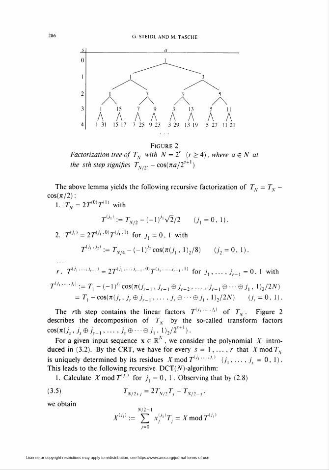
Figure 2
Factorization tree of TN with N = 2r (r > 4), where a G N at
the sth step signifies TN,V - cos(na/2s+l)
The above lemma yields the following recursive factorization of TN = TN
cos(n/2):1. T„ = 2TmT{l> with
TU^:=TN¡2-(-\)J'y/2/2 (j, =0,1).
2Tu"0)Tu"l] for 7, =0, 1 with"(7,)
'Y'iJ\ - Ji> ._ T-1
N/4l);2cos(7r(7,,l)2/8) (72 = 0,1).
r. Tu>.j'-<] = 2TU<.jr->^TUi.>'-",) for 7,, ... ,7,_, =0, 1 with
T(7,.1,) ._r, -(-\)Jrcos(n(jr_],jr_[®jr_2,... ,;r_,e---e;1, i)2/2/v)
= r, -cos(7r(7r,yreyr_,,... ,;,.©■■■©;,, i)2/2/v) (jr = o, l).
The nh step contains the linear factors rly'.Jr of 7^. Figure 2
describes the decomposition of TN by the so-called transform factors
cos(7t(7ç, js © js_{, ... , js © • • • ©7,, 1 )2/2i+1 ).
For a given input sequence x G E , we consider the polynomial X intro-
duced in (3.2). By the CRT, we have for every s = 1, ... , r that .Ymod7\
is uniquely determined by its residues XmodTiJ'.J- (jx, ... , js = 0, 1).
This leads to the following recursive DCT(Ar)-algorithm:
1. Calculate AmodrU|) for 7=0,1. Observing that by (2.8)
(3.5)
we obtain
X
T =1T T - T1 N/2+j L1Np.i] 1 N/2-j
N/2-i
U,)._ y x^T=XmodT°']
7=0
License or copyright restrictions may apply to redistribution; see https://www.ams.org/journal-terms-of-use

A POLYNOMIAL APPROACH TO FAST ALGORITHMS 287
with
Xj .-x, + (-l)J'xN/2V2/2
/V/21for 7 = 0,
<j - xN_j + (-l)J'xN/2+JV2 for j = 1,..., tV/2 - 1.
2. Calculate Xu,)modTUt'Ji) for 7,,72 = 0, 1. Using (3.5), with N/4
instead of N/2, we get
V/2-1
XUx.U) := Y xjJ>'J*)Tj = X(J>,modT4JiJi)
7=0
with
,(71.7,)
f 4A) + (-l);i^;ico8(»t/i. l)2/8) for 7 = 0,
Xj'] - xm-j + i-l)J2x{¿}lJ2cos(n(jl, l)2/8)
for7 = l,...,7V/4-l.
r. Calculate XUl.J'~'} modTu,'-'Jr) for j\ ,... , jr = 0, 1. This yields
the final result
xUl..-.Jr):=xUl,....J,) = xU..Á-,)modr(A.-.Á)
with
x,(7......Á) ..XpM.>Jr-l)
+ (-l)J'xjrJj\.-Jr-l)
cos(n(jr_l,jr_l®jr_2, ... ,jr_ 7,,l)2/2iV).
U"-'J'] = x,, forBy (3.3) and by the decomposition of TN , we see that x0 - ^k
the index k with
(3.6) k = Ur,jr®jr_i, ..., V '7,)2-
-©-
Figure 3
Flow graph for the DCT(8) with a := v/2/2, ß} := cos(nj/S)
and y i '■= cos(nj/l6)
License or copyright restrictions may apply to redistribution; see https://www.ams.org/journal-terms-of-use
288 G. STEIDL AND M. TASCHE
This describes the permutation of the output values. The (j{, ... , jr )2th com-
ponent of our output sequence is xk with k as in (3.6). Figure 3 shows the
flow graph of the DCT(8).Simple considerations yield the computational complexity of our DCT-
algorithm. The 5th step of the algorithm requires 2S~ (N/2S) real multiplica-
tions and 25~1(37V/2Î - 1) real additions. Thus, our DCT(N)-algorithm with
N = 2r (r G N) works with a total of
r
(3.7) MN = Y^\N/2S) = (N/2)r
real multiplications and
r
(3.8) AN =Y,2S-\3N/2S - 1) = (yV/2)(3r - 2) + 15=1
real additions. Hence, our polynomial algorithm has the same computational
complexity as the best-known DCT-algorithms [7, 8, 15].
The image x G CN of the DFT(N) of a real-valued sequence x G KA can
N-\
4. Cos-DFT and sin-DFT
iec" ofbe obtained by
i4A) xc k:=YxjC0Si2nkJ/N) (k = 0,...,N-\),7=0
N-\
(4-2) xs<k:=Yxjsini27ikj/N) (k = 0, ... , N - 1),7=0
and by
xk = xc,k ~ ixs,k (k = 0, ... , N - I).
The mappings defined by (4.1) and (4.2) are called the discrete Fourier-cosine
transform of length N (cos-DFT(AO) and the discrete Fourier-sine transform of
length N (sin-DFT(AO), respectively. In this section, we present a polynomial
approach to the cos-DFT and the sin-DFT, which suggests fast algorithms for
both transforms.
Let M := [N/2\ . By
cos(2nk(N - j)/N) = cos(2nkj/N) (j,keZ),
(4.1) can be rewritten as
M
(4.3) ck:=xck=xcN_k = YcjCOs(2nkj/N) (k = 0,...,M)7=0
withfor 7 = 0 and 7 = A/if 2|/V,
, .= { *7
' \Xj + XN_j(7 = 0,..., M).
otherwise
License or copyright restrictions may apply to redistribution; see https://www.ams.org/journal-terms-of-use

A POLYNOMIAL APPROACH TO FAST ALGORITHMS 289
We call (4.3) the reduced cos-DFJ(N) . Similarly, by
sin(2nk(N - j)/N) = - sm(2nkj/N) (j,keZ),
it follows from (4.2) that
M
(4.4) sk:=xs k = -xsN_k = Ysjsini27tkJ/N) (k = l,...,M)7=1
withfO for7 = A/if2|/V, .
Sj-.c=\ . (7 = 1, ... , M).1 \ Xj - xN_j otherwise
Then (4.4) is said to be the reduced sin-DFT(Ar). Hence we can calculate the
cos-DFT(TV) (sin-DFT(TV)) by [tV/2] - 1 additions and by the reduced cos-
DFT(A/~) (sin-DFT(TV)). Here, \N/2] := min{k G Z : k > N/2}. In thefollowing, we deal with these reduced transforms.
In order to introduce a polynomial notation of the reduced cos-DFT, we
represent the input sequence c = (c0, ... , cM) GR + as the polynomial
M
7=0
Then we have by (2.1) that ck = C(cos(2nk/N)) (k = 0, ... , M), i.e.,
(4.5) ck = C(z) mod(z - cos(27rrí/W)) (k = 0,...,M).
By (2.11), we obtain a fast algorithm for the reduced cos-DFT(iV) if we split
C mod VM+[ stepwise into equivalent simultaneous remainders by using succes-
sive factorization of VM+[ together with the CRT, such that we get (4.5) in the
last step.
Analogously, we represent the input sequence s = (s{, ... , sM) G RM of the
reduced sin-DFT as the polynomial
M
(4.6) $ :=£*; tf,-i-7 = 1
Then we see by (2.2) that (4.4) can be expressed as
sk = sin(2nk/N)S(cos(27tk/N)) (k=l,...,M),
i.e.,
(4.7) sk = sin(27Trc/7V)S(z) mod(z - cos(2nk/N)) (k = \,...,M).
It follows from (2.11 ) and from the CRT that we can deduce a fast sin-DFT(N)
if we reduce S(z) mod(VM+l(z)/2(z - 1)) successively into equivalent simul-
taneous residues by applying polynomial factorizations of VM ,(z)/2(z - 1),
such that we ultimately obtain (4.7).
For even TV g N, (4.6) and (4.7) can be simplified to
M-\
(4.8) S=ESJUJ-1>7=1
License or copyright restrictions may apply to redistribution; see https://www.ams.org/journal-terms-of-use

290 G. STEIDL AND M. TASCHE
(4.9) sk = sin(2nk/N)S(z) mod(z - cos(2nk/N)) (k = \, ... , M - \),
since sM = 0. By (2.4), we get a fast algorithm for the reduced sin-DFT(iV)
with even N G N by splitting S mod UM_] stepwise, such that we obtain (4.9)
in the end.
5. Fast algorithms for reduced cos-DFT and sin-DFT
In this section, we assume N g N divisible by 4. Set M := N/2. Based on
the factorization
(*•') "M-l = ^V^MIl)^Mß-\ — 2TM/2UM/2_l ,
which follows immediately from (2.7), we show that the reduced cos-DFT can be
decomposed into the reduced cos-DFT(Af/2) and the DCT(tV/4) . The reduced
sin-DFT can be handled analogously. This verifies a result in [15] from the
polynomial point of view.
By (2.12), (5.1), and by the CRT, Cmod VM+[ is completely determined by
its residues Cmod TM/2 and CmodVM/2+] . First we evaluate Cmod TM/2 by
polynomial reductions. By T- = -TM_¡ mod TM/2 (j = 0, ... , M/2 - 1), we
verify that
A//2-1
(5.2) C(1):= Y cj)Tj = CmodTM/27=0
with ¿P :=cj-cM_j (7 = 0, ..., A//2-1). Since by (2.12), (5.1) and (2.3),
è2k+\ = iic modVM+\)modTM/2) mod(r, - cos(2^(2ri + 1)/tV))
= C(1) mod^, -cos(7r(2¿; + \)/M)) (k = 0,... ,M/2- 1),
the output values with odd indices of the reduced cos-DFT(Ar) can be calculated
by M/2 additions and by the DCT(M/2) given by (5.2).On the other hand, by (2.9), we have T- = T^^ mod VM,2+i Ür.= 0, ... ,
M/2 - 1), so that Cmod VM,2+\ IS obtained by
M/2
(5.3) C(2):=£c<2)r, = Cmod^/2+17=0
with cf} := Cj + cM_j (7 = 0,..., M/2 - 1 ), cM]/2 := cMj2. Then we have by
(2.12), (5.1), and (2.4) that
c2k = ((C mod VM+l) modK^^,) mod(r, - cos(2n(2k)/N))
= C{2) mod(T{ - cos(2nk/M)) (k = 0, ... , M/2).
Hence, we get the output values with even indices of the reduced cos-DFT(A/)
by M/2 additions and by the reduced cos-DFT(tV/) determined in (5.3).
License or copyright restrictions may apply to redistribution; see https://www.ams.org/journal-terms-of-use

A POLYNOMIAL APPROACH TO FAST ALGORITHMS 291
Turning to the reduced sin-DFT, we take a similar approach. By (5.1) and
by the CRT, S mod UM_, is completely determined by its residues S mod TM/2
and S mod UM ,2_, . Considering that, by (2.10), [/_, = UM_j_xmodTM,2
(j = 1, ... , M/2), we find that 5 mod TM/2 is given by
M/2
S{i)-=YSJ)U^=Sm0dTM/27=1
with s{jl) := Sj + sM_j (j = 1, ... , M/2 - 1), sM]/2 := sM/2. Instead of 5(1!
we consider
M/2-l
(5.4) 5(":= 2 4"r;.7=0
with s{}] := s(M]l2_j (7 = 0,..., M/2 - 1). Then from
sin(27T(2A: + \)/N)Uj_x(cos(n(2k + 1)/M)) = sin(2^(2Ä: + \)j/N)
= (-\)kco%(2Tt(2k+\)(MI2-j)IN) = (-l)kTM/2_J(cos(n(2k + l)/M))
one verifies that
s2k+i = sin(2rt(2/c+ \)/N)((Smod i7M_1)modrA//2)
mod(r, -cos(2^(2ri+ 1)/tV)
= sin(2?r(2rx + \)/N)S{U mod(Tl -cos(n(2k+ 1)/M))
= (-l)A5<"mod(ri -cos(7i(2ri + \)/M)) (k = 0,..., M/2- 1).
Consequently, we obtain the output values with odd indices of the reduced
sin-DFT(A0 by M/2 - 1 additions and by the DCT(M/2) given by (5.4),where we have to change the sign of the output values with indices congruent 3
modulo 4.
Next, by (2.10), we have £/._, = -UM_j_l mod UMjl_x (j = \, ... , M/2-
1 ). Using this property, we form
M/2- 1
(5.5) S{2):= Y *?V.=5modtV/2-i/=i
(2)with S: := Sj - sXi_j (7 = 1,..., M/2 - 1). Now we conclude from
s2k = sin(27i(2k)/N)((Smod UM_X) mod UM/2_x)mod(T{ - co$(2n(2k)/N))
= sin(2?r/:/M)S(2)mod(ri - cos(27Tri/M)) (k = 1,... , M/2- 1),
that the output values with even indices of the reduced sin-DFT(Ar) can be
evaluated by M/2 - 1 additions and by the reduced sin-DFT(M) determined
in (5.5).
License or copyright restrictions may apply to redistribution; see https://www.ams.org/journal-terms-of-use

292 G. STEIDL AND M. TASCHE
COS-DFT(/V)
j [N/2-1]
reduced cos-DFT(/V)
[ N/4]^^\^[ N/4]
DCT(A//4) reduced cos-DFT(A//2)
reduced cos-DFT(4«)
DCT(u) reduced cos-DFT(2h)
Figure 4
Recursive computation of the cos-DFT'(tV) with N = 2ru (r >
2 ; u odd) ([■] signifies the number of additions per step)
Let N = 2r (r > 2). Then we can use the above reduction successively
for the reduced cos-DFT(25) (reduced sin-DFT(2i)) with s = r, ... ,2. This
results in the computation of the cos-DFT(yV) (sin-DFT(YV)) using only DCT's
and some additions. See Figure 4 with u := 1.
The numbers MCN and M^ of real multiplications and the numbers ACN
and ASN of real additions to perform the cos-DFT(A^) and the sin-DFT(TV),
respectively, follow directly from Figure 4, (3.7) and (3.8). For N = 2r (r>2),
one obtains
r-2
K = K = J2Mr = W4)(r- 3) + 1,5=1
r-2 r-2
ACN = TV/2 - 1 + 2 Y 2' + Y ^? + 2 = (#/4)(3r - 5) + r + 2,5=0 5=1
r-2 r-2
4 = tV/2 - 1 + 2£(2S - \) + Y^r = W4)(3r - 5) -r+ 2.5=0 5=1
Consequently, the DFT(tV) of a real-valued sequence computed by our method
requires
M; = MCN + MSN = (N/2)(r - 3) + 2 ,
ArN = ACN + ASN = (/V/2)(3r - 5) + 4
License or copyright restrictions may apply to redistribution; see https://www.ams.org/journal-terms-of-use

A POLYNOMIAL APPROACH TO FAST ALGORITHMS 293
real multiplications and real additions, respectively. Further, by
N-\ N-\
xk= Y R-eixj) cos(2nkj/N) - Y Im(Xj)sm(27ikj/N)7=0 7=1
jjtN/2
(N-\ N-\
Y^miXj)cos(2nkj/N)+ Y Re(Xj)sin(2nkj/N)7=0 J=\
jftN/2
(k = 0,...,N-\),
the number of real operations of the DFT( N) of a complex-valued sequence is
given by
MN = 2MrN = N(r - 3) + 4, AN = 2ÄN + 2(N -2) = 3N(r - 1) + 4.
Compared with other DFT-algorithms, we conclude that our polynomial algo-
rithm works with the same computational complexity as the algorithm in [15]
and the split-radix algorithm [3, 14].
6. Fast algorithm for the DCT(3Ar)
The polynomial representations of the DCT(N), the cos-DFT(Ar), and the
sin-DFTiA7) in §§3 and 4 open new possibilities for the derivation of fast al-
gorithms for these transforms for various lengths N by applying the CRT in
combination with the factorizations (2.5), (2.6), and (2.7) of Chebyshev poly-
nomials, or in combination with the factorization (2.11). The reductions of
polynomials of the form (3.2) or (4.8) modulo Chebyshev polynomials in such
algorithms can be performed only by (2.8), (2.9), and (2.10). In order to illus-
trate these general considerations, we suggest a new polynomial algorithm for
the DCT(3/V).We consider the DCT(3yV) (N gN), i.e., for given
3N-1
X'= E XjTj m0dT3N>
7=0
we have to evaluate
xk = X(z) mod(z - cos(n(2k + l)/6N)) (k = 0, ... , 3tV- 1).
By (2.5), T}N factors as
T3N = 4{TN-V3/2)TN(TN + y/3/2),
so that X mod TiN is completely determined by the residues X mod TN and
Xmod(TN ± 1/3/2). Considering that by (2.5) and (2.8)
T = 2T2 - 112N Z-1 N ' '
7^ = 27^.-/„_,,
T2N+j = i< - 1)7} - 27V7„_, (7 = 1, ... , TV - 1),
we obtain the following recursive algorithm.
License or copyright restrictions may apply to redistribution; see https://www.ams.org/journal-terms-of-use

294 G. STEIDL AND M. TASCHE
First, we calculate X mod TN by
(6.1) X{0):=':£x?)Tj = XmodTN
with
7 7
7=0
(0) .. Í xo ~ X2N for7 = 0,
1 \x- x2N_. - x1N,,. for 7 = 1, ... , /V - 1.v7 -^2V-7 ■A'27V+7
Since by (2.3), 7A, has the roots cos(7r(2/c + l)/2/V) = c s(«(2(3ik+l) + l)/6iV)
(/c = 0, ... , N - 1 ), we obtain
xik+x = X{0) mod(Tx -cos(n(2k+ l)/2N)) (k = 0, ... , N - I).
Next, we form Xmod(TN ± \ß/2) as follows:
/v-i(6.2) X{[) := Y Xjl)Tj = *mod(7„ - VÏ/2)
7=0
with
(1) _ J A0 "•" A2JVXj .-
+ x2N/2 + xN\ß/2 for7 = 0,
■j - x2N_j + 2x2N+j + \fï(xN+J - x3N_j) for j = 1,..., N - 1,
and
N-\
(6.3) Xi2) := Y xTTj = Xmod(TN + VÎ/2)7=0
with
v(2) ._ j •*0~rA2/v/Xj .-
+ x2N/2-xNV3/2, for 7 = 0,
XJ - X2N-j + 2X2N+j - ^iXN+j - XiN-j) for 7 = 1 , • •. , TV - 1 .
By (2.6), the zeros of TN - \H>/2 and of TN + \fi>/2 are given by
{cos((7r/6 + 27i/i)/TV):/c = 0, ... , N- 1}
= {cos(7r(2(6/c) + 1)/6tV) , cos(tt(2(6/c' + 5) + 1)/6tV) :
k = 0, ... ,M;k' = 0,... ,M'}
and by
{cos(5?r/6 + 2itk/N) :k = 0, ... , N -1}
= {cos(n(2(6k + 2)+ 1)/6tV) , cos(n(2(6k' + 3) + 1)/6tV) :
k = 0,...,M;k' = 0,...,M'},
License or copyright restrictions may apply to redistribution; see https://www.ams.org/journal-terms-of-use

A POLYNOMIAL APPROACH TO FAST ALGORITHMS 295
respectively, where M := [tV/2] - 1 and M1 := [tV/2J - 1. Hence, we get by
(6.2) and (6.3) that
x6k = Xw mod(Tx-cos(n(l2k+l)/6N)) (k = 0,...,M),
x6k+5 = X{l) mod(Tx-cos(n(l2k+ll)/6N)) (k = 0, ... , M'),
x6k+2 = X{2) mod(Tx-cos(n(l2k + 5)/6N)) (k = 0,...,M),
x6k+3 = X{2) mod(Tl-cos(n(\2k + 7)/6N)) (k = 0, ... , M').
As a result, we have decomposed the DCT(3tV) into the DCT(tV) given by
(6.1) and into the modified DCT(tV)'s determined by (6.2) and (6.3), with a
total of 2tV multiplications and 6tV - 2 additions. Obviously, using (2.6)
instead of (2.5), these modified DCT's can be handled similarly as the usual
DCT. We have only to change the transform factors in the multiplications.
We now combine this idea with the developments of the previous sections.
Let N = 2r (r>2). Then by (3.7) and (3.8), we can perform the DCT(3tV)
with
MiN = 3MN + 2N = (N/2)(3r + 4), Äw = 3Í„ + 6tV-2 = (N/2)(9r + 6)+\
real operations. Using the decompositions in §5 (see Figure 4), we obtain the
following computational complexity for the cos-DFT(3tV) and for the sin-
DFT(3tV) :
r-2
M¡N = Msw = Y M,.? + 2 = (TV/4)(3r - 5) + 3,5=0
r-2 r-2
A\N = 3tV/2 -1 + 2^3-2* + YA~i-2* + 8 = W4)(9r - 3) + r + 6,5=0 5=0
r-2 r-2
AsiN = 3tV/2 - 1 + 2 £(3 -2s - 1) + Y^-is +2 = W4)^ - 3) - r + 2.5=0 5=0
Finally, we see that the DFT(3tV) requires
M[N = (7V/2)(3r- 5) + 6, Mw = N(3r- 5) + 12
real multiplications and
A\N = (N/2)(9r - 3) + 8 , A}N = N(9r + 3) + 12
real additions. This coincides with the number of real operations for the com-
putation of the DFT(3 • 2r) (r > 2) by combining the prime factor algorithm,
the split-radix algorithm and the Rader algorithm [1, 14].
Bibliography
1. A. V. Aho, J. E. Hopcroft, and J. D. Ullmann, The design and analysis of computer algo-
rithms, Addison-Wesley, Reading, Mass., 1976.
2. G. Bruun, z-transform DFT filters and FFTs, IEEE Trans. Acoust. Speech Signal Process.
26(1978), 56-63.
License or copyright restrictions may apply to redistribution; see https://www.ams.org/journal-terms-of-use

296 G. STEIDL AND M. TASCHE
3. P. Duhamel, Implementation of "split-radix" FFT algorithms for complex, real and real-
symmetric data, IEEE Trans. Acoust. Speech Signal Process. 34 (1986), 285-295.
4. D. Garbe, On the level of irreducible polynomials over Galois fields, J. Korean Math. Soc.
22(1985), 117-124.
5. I. S. Gradshtein and I. M. Ryzhik, Tables of integrals, sums, series and products, Nauka,
Moscow, 1971. (Russian)
6. M. T. Heideman and C. S. Burrus, On the number of multiplications necessary to compute
a length-2" DFT, IEEE Trans. Acoust. Speech Signal Process. 34 (1986), 91-95.
7. H. S. Hou, A fast recursive algorithm for computing the discrete cosine transform, IEEE
Trans. Acoust. Speech Signal Process. 35 (1987), 1455-1462.
8. B. G. Lee, A new algorithm to compute the discrete cosine transform, IEEE Trans. Acoust.
Speech Signal Process. 32 (1984), 1243-1245.
9. M. J. Narasimha and A. M. Peterson, On computing the discrete cosine transform, IEEE
Trans. Comm. 26 (1978), 934-936.
10. H. J. Nussbaumer, Fast Fourier transform and convolution algorithms. Springer, Berlin-
Heidelberg-New York, 1981.
U.S. Paszkowski, Numerical application of Chebyshev polynomials and series, Nauka, Moscow,
1983. (Russian)
12. T. J. Rivlin, The Chebyshev polynomials, Wiley, New York-London-Sydney-Toronto, 1974.
13. H. V. Sorensen, D. L. Jones, C. S. Burrus, and M. T. Heideman, On computing the discrete
Hartley transform, IEEE Trans. Acoust. Speech Signal Process. 33 (1985), 1231-1238.
14. H. V. Sorensen, D. J. Jones, M. T. Heideman, and C. S. Burrus, Real-valued fast Fourier
transform algorithms, IEEE Trans. Acoust. Speech Signal Process. 35 (1987), 849-863.
15. M. Vetterli and H. J. Nussbaumer, Simple FFT and DCT algorithms with reduced number
of operations, Signal Process. 6 (1984), 267-278.
16. S. Winograd, On computing the discrete Fourier transform, Math. Comp. 32 (1978), 175—
199.
17._Arithmetic complexity of computations, CBMS Regional Conf. Ser. in Math., vol. 33,
SIAM, Philadelphia, 1980.
Fachbereich Mathematik, Universität Rostock, Universitätsplatz 1, 0-2500 Rostock,
Germany
License or copyright restrictions may apply to redistribution; see https://www.ams.org/journal-terms-of-use