a plane wave and projector augmented wave implementation...
TRANSCRIPT

A plane wave and projectoraugmented wave
implementation of DFT+DMFTBernard Amadon
CEA, DAM, DIF, F-91297 Arpajon, France
In Collaboration with J. Bieder, A. Georges, F. Jollet, F. Lechermann, A. I. Lichstenstein, M. Torrent
FPLMTO 2012, IPCMS Strasbourg – p.1/45

Outline of the presentation
• Choice of the basis and local orbitals.• The PAW framework• Description of the actual calculation• Some tests/examples.• Conclusion.
FPLMTO 2012, IPCMS Strasbourg – p.2/45

Localization of 3d, 4f and 5f electrons
3d and4f are orthogonal to other orbitals only through theangularpart.
0
0.5
spd
rφ(r)
0
0.5
0 0.5 1 1.5r (Å)
0
0.5
V (3d)
Nb (4d)
Ta (5d)
V (3d)
Nb (4d)
Ta (5d)
V (3d)
Nb (4d)
Ta (5d)
V (3d)
Nb (4d)
Ta (5d)
V (3d)
Nb (4d)
Ta (5d)
V (3d)
Nb (4d)
Ta (5d)
V (3d)
Nb (4d)
Ta (5d)
0
0.5
1
sdf
rφ(r)
0 1 2r(Å)
0
0.5
1
Th (5f)
Ce (4f)
FPLMTO 2012, IPCMS Strasbourg – p.3/45

DFT+U and the Dynamical Mean Field Theory (DMFT)
• DFT+U⇒ To describe interactions in solids with static mean fieldtheoryMain idea: An electron is described, in the effective field ofall theother electrons.⇒ Self-consistent Hartree Fock problem.
[Anisimov V I, Poteryaev A I, Korotin M A, Anokhin A O and Kotliar G J. Phys.: Condens. Matter 9
735967 (1997)]
FPLMTO 2012, IPCMS Strasbourg – p.4/45
DFT+U and the Dynamical Mean Field Theory (DMFT)
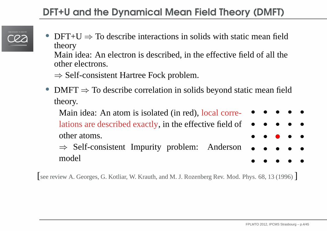
• DFT+U⇒ To describe interactions in solids with static mean fieldtheoryMain idea: An electron is described, in the effective field ofall theother electrons.⇒ Self-consistent Hartree Fock problem.
• DMFT ⇒ To describe correlation in solids beyond static mean fieldtheory.Main idea: An atom is isolated (in red),local corre-lations are described exactly, in the effective field ofother atoms.⇒ Self-consistent Impurity problem: Andersonmodel
[see review A. Georges, G. Kotliar, W. Krauth, and M. J. Rozenberg Rev. Mod. Phys. 68, 13 (1996)]
FPLMTO 2012, IPCMS Strasbourg – p.4/45

The DFT+DMFT schemeA Self-consistent DFT+DMFT scheme in the Projector Augmented Wave : Applications to Cerium, Ce O and Pu
Σ = G−10 − G−1
impG−10 = Σ + G−1
imp
Gimpn(r) Σ
Glatt
GHKS−DFT problem
Impurity
Self-consistencycondition
DFT+DMFT Loop over density
〈χRkm|Ψkν〉
fDFT+DMFTν,ν′,k
DMFT for fixed n(r)
ǫKS−DFTν,k G0
Gimp
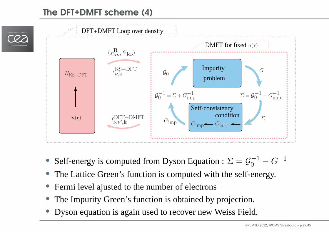
Figure 1. Fully Self-consistent DFT+DMFT scheme adapted to the Projected Local Orbital schemeused in our implementation. For a fixed electronic density, the DMFT Loop is represented in blue. Itcontains two steps: Firstly, the impurity model is solved to compute the Green function and the self-energy . Secondly the lattice Green function is computed from the impurity self-energy, andthe self-consistency condition states that the local Green function is also the impurity Green function.When this DMFT loop is converged, one can compute the lattice Green function and the non diagonaloccupations in the Kohn Sham Bloch basis. The occupations are used to compute the total electronicdensity (in practice, its PW and PAW components) thanks to Eq. 2.7. From this density, the Kohn ShamDFT Hamiltonian is build and diagonalized. The new KS bloch wave functions, and the eigenvalues arethen used to compute the Green function (Eq. 2.5). Then a new DMFT loop is performed. This cycle(in pink) is repeated until convergence of the density.
is the density operator in these equations.Then, the DFT Hamiltonian is built and diagonalized: new KS eigenvalues and eigenfunctions
are extracted. A special care is taken to obtain the new KS bands with a good accuracy for eachnew electronic density, especially for unoccupied KS states. Then, projections 2.1 are recomputed tobuild Wannier functions for the next DMFT loop. KS eigenvalues are also used to compute the Greenfunction using 2.5.
Peculiarities of the PAW formalism for the computation of the electronic density are describedin Appendix A.
2.3. Calculation of Internal Energy in DFT+DMFTThe DFT+DMFT formalism can be derived from a functional [45] of both the local density andthe local Green’s function [46]. The internal energy can be derived and one obtain the general
FPLMTO 2012, IPCMS Strasbourg – p.5/45

DMFT in the Kohn Sham basis
• Let’s choose the Bloch basis as the basis for one electron quantities.• One electron Hamiltonian:
HKS =∑
ν,k
|Ψkν〉 εkν 〈Ψkν |
• A basis set for one electron quantities:|Bkα〉.
• The matrix element on the Hamiltonian can thus be computed as:
HKS,αα′(k) = 〈Bkα|HKS|Bkα′〉
=∑
ν
〈Bkα|Ψkν〉 εkν 〈Ψkν |Bkα′〉 .
• A definition for d/f local orbitals, let’s call them|χR
km〉. (m is anangular momentum index)
FPLMTO 2012, IPCMS Strasbourg – p.6/45

DMFT in the Kohn Sham basis
• Let’s choose the Bloch basis as the basis for one electron quantities.• One electron Hamiltonian:
HKS =∑
ν,k
|Ψkν〉 εkν 〈Ψkν |
• Basis set for one electron quantities:|Ψkν〉.
• The matrix element on the Hamiltonian can thus be computed as:
HKS,νν′(k) = 〈Ψkν |H|Ψkν〉
= εkνδν,ν′
• A definition for d/f local orbitals, let’s call them|χR
km〉. (m is anangular momentum index)
FPLMTO 2012, IPCMS Strasbourg – p.6/45
DMFT in the Kohn Sham basis (2)
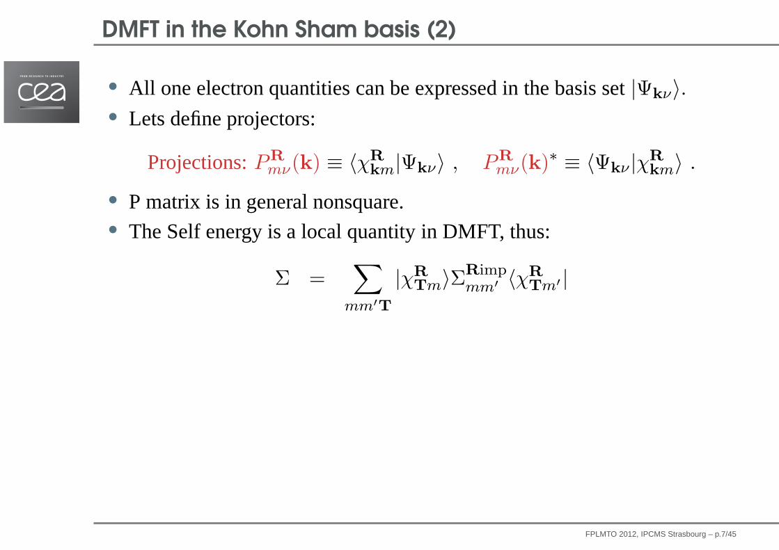
• All one electron quantities can be expressed in the basis set|Ψkν〉.
• Lets define projectors:
Projections:PR
mν(k) ≡ 〈χR
km|Ψkν〉 , PR
mν(k)∗ ≡ 〈Ψkν |χR
km〉 .
• P matrix is in general nonsquare.• The Self energy is a local quantity in DMFT, thus:
Σ =∑
mm′T
|χR
Tm〉ΣRimpmm′ 〈χ
R
Tm′ |
FPLMTO 2012, IPCMS Strasbourg – p.7/45

DMFT in the Kohn Sham Bloch basis (3)
Thus
∆Σαα′(k, iωn) = 〈Ψkν |Σ(k)|Ψkν〉
=∑
mm′
PR
mν(k)∗ΣRimpm,m′ P
R
mν(k).
The lattice Green’s functionGα,α′(k, iωn) can be expressed in thecomplete Bloch BasisΨkν . and projected to compute the local (impurity)Green’s function.
Gimpmm′(iωn) =
∑
k
∑
νν′
PR
mν(k)PR
m′ν′(k)∗ ×
×
[(iωn + µ − εkν)I −∆Σ(k, iωn)]−1
νν′
,
FPLMTO 2012, IPCMS Strasbourg – p.8/45

Choice of the basis set and local orbitals
• The local atomic-like orbitalsχR
km will in general have adecomposition involvingall Bloch bands (closure relation)
|χR
km〉 =∑
ν
〈Ψkν |χR
km〉|Ψkν〉 =
[∑
ν
|Ψkν〉〈Ψkν |
]|χR
km〉
• If the basis set is restricted to a limited number of KS statesin thewindow energyW :
|χR
km〉 ≡∑
ν∈W
〈Ψkν |χR
km〉|Ψkν〉 = PR
mν(k)∗|Ψkν〉
• |χR
km〉 need to be orthonormalized to give true Wannier functions|wR
km〉.
OR,R′
m,m′(k) = 〈χR
km|χR′
km′〉 =∑
ν
PR
mν(k)PR′
m′ν(k)∗
FPLMTO 2012, IPCMS Strasbourg – p.9/45

Choice of the basis set and local orbitals
• |wR
km〉 is thus obtained though:
|wR
km〉 =∑
R′,m′
[O(k)]−1/2
R,R′
m,m′
|χR′
km′〉
⇒ Projections accordingly renormalized.
⇒ The localized basis|wR
km〉 depends on the energy windowsW .
• |wR
km〉 less localized than initialχR
km since the basis has asmallerenergy range.
• If |wR
km〉 is chosen (through the window of energy),the wholeframework is exact: There is no finite basis effect.• 〈wR
km|Ψkν〉 = 0 if ν /∈ W.⇒ No convergence as a function of the size of the basis.
FPLMTO 2012, IPCMS Strasbourg – p.10/45

Basis set and local orbitals: Physical considerations
A reminder: hybridization in a diatomic molecule (oversimplified)
H or V
F or O
FPLMTO 2012, IPCMS Strasbourg – p.11/45

An oversimplified derivation for the diatomic molecule VO
φV
φOε1
Ψ1 = αφO + βφV β ≪ α
ε2
Ψ2 = βφO − αφV β ≪ α
Two windows of energy are possible to compute|χ〉 =
∑W〈Ψi|φV 〉|Ψi〉
• If only ε2 is included, the correlated wavefunction is|χ〉 = |Ψ2〉 = β|φO〉 − α|φV 〉 and contains an Oxygencontribution
• If only ε1 andε2 is included, the correlated wavefunction is|χ〉 =
∑i〈Ψi|φV 〉|Ψi〉 = |φV 〉 and is much more localized.
FPLMTO 2012, IPCMS Strasbourg – p.12/45

Formalism: DFT+DMFT implementation, LMTO
• LMTO ASA |χl,l′,m,m′(k)〉 (Andersen 1975).• LMTO’s are an optimized atomic orbital Bloch basis.• The local correlated subspace is thus asubset of the LMTO basis
Bkα.• |χl=2,l′=2,m,m′(k)〉 for d orbitals.
• First implementation in DMFT: Lichtenstein and Katsnelson1998, Anisimov et al 1997
• Fast, efficient, but method dependent.
FPLMTO 2012, IPCMS Strasbourg – p.13/45

The Projector-Augmented Wave (PAW) method: introduction
• Norm conserving pseudopotentials• Electronic density iserroneous.• Transferability might be thus questionnable• High number wave needed.
• A solution• A better descriptionof all electron wavefunctions nodes
|Ψ〉 = |Ψ〉 +∑
i
ci(|φi〉 − |φi〉) with ci = 〈 ˜pi|Ψ〉
• Relax the constraints over norm of pseudopotentials ("ultrasoft")• PAW Blöchl PRB 1994
• No pseudopotential approximation• Use an augmentation around atomsto have a correct shape for
wavefunctions near the nucleus.• Keep frozen core approximation (can be controlled)
FPLMTO 2012, IPCMS Strasbourg – p.14/45

The Projector Augmented Wave Method
12PAW method and DFPT
-48
nn ~ =
n nnnnnnn AfAfA ~~ *
!"
6- ,
$ ! $!
RRR nnnn rrrr 11
~~R
RR EEEE 11~~
* 48
%&
n~τ=(
iiφ+ nip ~~
)i~φ−
PAW• Efficiency with respect to usual plane wave calculations.• Accuracy: nodal structure of valence wfc are reproduced.• Flexibility: energy of several structures can be compared with the
same basis.• Frozen core approximation can be controlled.
From M. Torrent and F. Jollet Torrent, Jollet, Bottin, Zerah, Gonze CMS 2008
FPLMTO 2012, IPCMS Strasbourg – p.15/45

How to construct atomic data for PAW
• Solve All Electrons Atomic problem⇒ ϕi(r)
• Pseudize local pseudopotentialVloc.• Pseudize partial waveϕi(r).• Build projectorspi(r)..
FPLMTO 2012, IPCMS Strasbourg – p.16/45

Solve All Electrons Atomic problem⇒ ϕi(r)
• Solve atomic Schrödinger equation to compute electronicdensity. GetVae(r)
• Choose an energy setǫi and solve the Schrödinger equation.Getϕi(r) for eachǫi
FPLMTO 2012, IPCMS Strasbourg – p.17/45

Compute pseudo functions
FPLMTO 2012, IPCMS Strasbourg – p.18/45
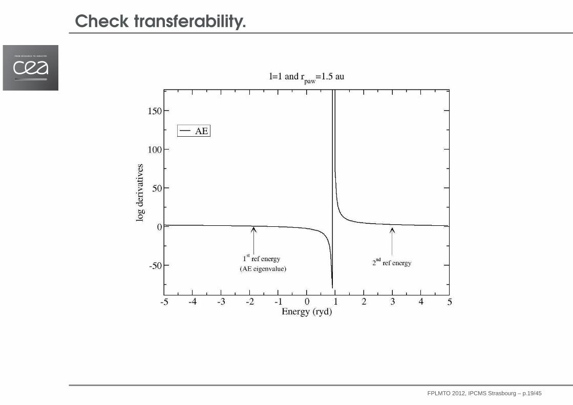
Check transferability.
FPLMTO 2012, IPCMS Strasbourg – p.19/45

Check transferability.
FPLMTO 2012, IPCMS Strasbourg – p.20/45

Check transferability.
FPLMTO 2012, IPCMS Strasbourg – p.21/45

The DFT+DMFT scheme (1): a practical calculationA Self-consistent DFT+DMFT scheme in the Projector Augmented Wave : Applications to Cerium, Ce O and Pu
Σ = G−10 − G−1
impG−10 = Σ + G−1
imp
Gimpn(r) Σ
Glatt
GHKS−DFT problem
Impurity
Self-consistencycondition
DFT+DMFT Loop over density
〈χRkm|Ψkν〉
fDFT+DMFTν,ν′,k
DMFT for fixed n(r)
ǫKS−DFTν,k G0
Gimp
Figure 1. Fully Self-consistent DFT+DMFT scheme adapted to the Projected Local Orbital schemeused in our implementation. For a fixed electronic density, the DMFT Loop is represented in blue. Itcontains two steps: Firstly, the impurity model is solved to compute the Green function and the self-energy . Secondly the lattice Green function is computed from the impurity self-energy, andthe self-consistency condition states that the local Green function is also the impurity Green function.When this DMFT loop is converged, one can compute the lattice Green function and the non diagonaloccupations in the Kohn Sham Bloch basis. The occupations are used to compute the total electronicdensity (in practice, its PW and PAW components) thanks to Eq. 2.7. From this density, the Kohn ShamDFT Hamiltonian is build and diagonalized. The new KS bloch wave functions, and the eigenvalues arethen used to compute the Green function (Eq. 2.5). Then a new DMFT loop is performed. This cycle(in pink) is repeated until convergence of the density.
is the density operator in these equations.Then, the DFT Hamiltonian is built and diagonalized: new KS eigenvalues and eigenfunctions
are extracted. A special care is taken to obtain the new KS bands with a good accuracy for eachnew electronic density, especially for unoccupied KS states. Then, projections 2.1 are recomputed tobuild Wannier functions for the next DMFT loop. KS eigenvalues are also used to compute the Greenfunction using 2.5.
Peculiarities of the PAW formalism for the computation of the electronic density are describedin Appendix A.
2.3. Calculation of Internal Energy in DFT+DMFTThe DFT+DMFT formalism can be derived from a functional [45] of both the local density andthe local Green’s function [46]. The internal energy can be derived and one obtain the general
• First step: Make a converged DFT calculation.• WavefunctionsΨkν and Eigenvaluesεkν are available.• Unoccupied wavefunctions must be accurately computed in
order to be used in the DMFT calculation.
FPLMTO 2012, IPCMS Strasbourg – p.22/45

Diagonalise the Hamiltonian
• Solve DFT self-consistently• Diagonalize the Hamiltonian with empty states• Get Eigenvalues and eigenvectors.
FPLMTO 2012, IPCMS Strasbourg – p.23/45
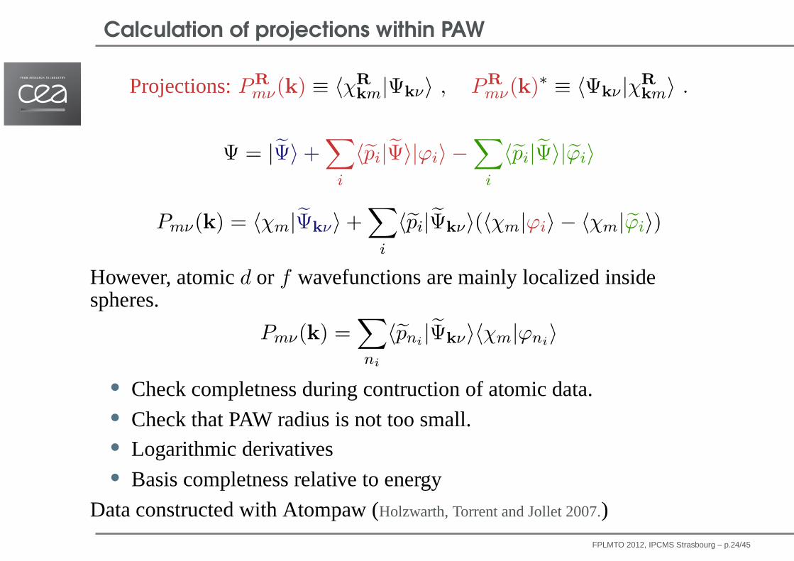
Calculation of projections within PAW
Projections:PR
mν(k) ≡ 〈χR
km|Ψkν〉 , PR
mν(k)∗ ≡ 〈Ψkν |χR
km〉 .
Ψ = |Ψ〉 +∑
i
〈pi|Ψ〉|ϕi〉 −∑
i
〈pi|Ψ〉|ϕi〉
Pmν(k) = 〈χm|Ψkν〉 +∑
i
〈pi|Ψkν〉(〈χm|ϕi〉 − 〈χm|ϕi〉)
However, atomicd or f wavefunctions are mainly localized insidespheres.
Pmν(k) =∑
ni
〈pni|Ψkν〉〈χm|ϕni
〉
• Check completness during contruction of atomic data.• Check that PAW radius is not too small.• Logarithmic derivatives• Basis completness relative to energy
Data constructed with Atompaw (Holzwarth, Torrent and Jollet 2007.)
FPLMTO 2012, IPCMS Strasbourg – p.24/45

The DFT+DMFT scheme (2)A Self-consistent DFT+DMFT scheme in the Projector Augmented Wave : Applications to Cerium, Ce O and Pu
Σ = G−10 − G−1
impG−10 = Σ + G−1
imp
Gimpn(r) Σ
Glatt
GHKS−DFT problem
Impurity
Self-consistencycondition
DFT+DMFT Loop over density
〈χRkm|Ψkν〉
fDFT+DMFTν,ν′,k
DMFT for fixed n(r)
ǫKS−DFTν,k G0
Gimp
Figure 1. Fully Self-consistent DFT+DMFT scheme adapted to the Projected Local Orbital schemeused in our implementation. For a fixed electronic density, the DMFT Loop is represented in blue. Itcontains two steps: Firstly, the impurity model is solved to compute the Green function and the self-energy . Secondly the lattice Green function is computed from the impurity self-energy, andthe self-consistency condition states that the local Green function is also the impurity Green function.When this DMFT loop is converged, one can compute the lattice Green function and the non diagonaloccupations in the Kohn Sham Bloch basis. The occupations are used to compute the total electronicdensity (in practice, its PW and PAW components) thanks to Eq. 2.7. From this density, the Kohn ShamDFT Hamiltonian is build and diagonalized. The new KS bloch wave functions, and the eigenvalues arethen used to compute the Green function (Eq. 2.5). Then a new DMFT loop is performed. This cycle(in pink) is repeated until convergence of the density.
is the density operator in these equations.Then, the DFT Hamiltonian is built and diagonalized: new KS eigenvalues and eigenfunctions
are extracted. A special care is taken to obtain the new KS bands with a good accuracy for eachnew electronic density, especially for unoccupied KS states. Then, projections 2.1 are recomputed tobuild Wannier functions for the next DMFT loop. KS eigenvalues are also used to compute the Greenfunction using 2.5.
Peculiarities of the PAW formalism for the computation of the electronic density are describedin Appendix A.
2.3. Calculation of Internal Energy in DFT+DMFTThe DFT+DMFT formalism can be derived from a functional [45] of both the local density andthe local Green’s function [46]. The internal energy can be derived and one obtain the general
• Fromεkν, compute DFT (LDA) Green’s function:
GBlochν,ν′ (iωn,k) = [(iωn + µ − εkν)I]
−1νν′
Gimpmm′(iωn) =
∑
k
∑
νν′
PR
mν(k)PR
m′ν′(k)∗GBlochν,ν′ (iωn,k)
FPLMTO 2012, IPCMS Strasbourg – p.25/45

The DFT+DMFT scheme (3)A Self-consistent DFT+DMFT scheme in the Projector Augmented Wave : Applications to Cerium, Ce O and Pu
Σ = G−10 − G−1
impG−10 = Σ + G−1
imp
Gimpn(r) Σ
Glatt
GHKS−DFT problem
Impurity
Self-consistencycondition
DFT+DMFT Loop over density
〈χRkm|Ψkν〉
fDFT+DMFTν,ν′,k
DMFT for fixed n(r)
ǫKS−DFTν,k G0
Gimp
Figure 1. Fully Self-consistent DFT+DMFT scheme adapted to the Projected Local Orbital schemeused in our implementation. For a fixed electronic density, the DMFT Loop is represented in blue. Itcontains two steps: Firstly, the impurity model is solved to compute the Green function and the self-energy . Secondly the lattice Green function is computed from the impurity self-energy, andthe self-consistency condition states that the local Green function is also the impurity Green function.When this DMFT loop is converged, one can compute the lattice Green function and the non diagonaloccupations in the Kohn Sham Bloch basis. The occupations are used to compute the total electronicdensity (in practice, its PW and PAW components) thanks to Eq. 2.7. From this density, the Kohn ShamDFT Hamiltonian is build and diagonalized. The new KS bloch wave functions, and the eigenvalues arethen used to compute the Green function (Eq. 2.5). Then a new DMFT loop is performed. This cycle(in pink) is repeated until convergence of the density.
is the density operator in these equations.Then, the DFT Hamiltonian is built and diagonalized: new KS eigenvalues and eigenfunctions
are extracted. A special care is taken to obtain the new KS bands with a good accuracy for eachnew electronic density, especially for unoccupied KS states. Then, projections 2.1 are recomputed tobuild Wannier functions for the next DMFT loop. KS eigenvalues are also used to compute the Greenfunction using 2.5.
Peculiarities of the PAW formalism for the computation of the electronic density are describedin Appendix A.
2.3. Calculation of Internal Energy in DFT+DMFTThe DFT+DMFT formalism can be derived from a functional [45] of both the local density andthe local Green’s function [46]. The internal energy can be derived and one obtain the general
• 1st iteration: DFT LDA Green’s function used as Weiss field• From Weiss FieldG0 m,m′, Anderson Impurity Model is solved
to get impurity Green’s functionGm,m′.
FPLMTO 2012, IPCMS Strasbourg – p.26/45
The DFT+DMFT scheme (4)A Self-consistent DFT+DMFT scheme in the Projector Augmented Wave : Applications to Cerium, Ce O and Pu
Σ = G−10 − G−1
impG−10 = Σ + G−1
imp
Gimpn(r) Σ
Glatt
GHKS−DFT problem
Impurity
Self-consistencycondition
DFT+DMFT Loop over density
〈χRkm|Ψkν〉
fDFT+DMFTν,ν′,k
DMFT for fixed n(r)
ǫKS−DFTν,k G0
Gimp
Figure 1. Fully Self-consistent DFT+DMFT scheme adapted to the Projected Local Orbital schemeused in our implementation. For a fixed electronic density, the DMFT Loop is represented in blue. Itcontains two steps: Firstly, the impurity model is solved to compute the Green function and the self-energy . Secondly the lattice Green function is computed from the impurity self-energy, andthe self-consistency condition states that the local Green function is also the impurity Green function.When this DMFT loop is converged, one can compute the lattice Green function and the non diagonaloccupations in the Kohn Sham Bloch basis. The occupations are used to compute the total electronicdensity (in practice, its PW and PAW components) thanks to Eq. 2.7. From this density, the Kohn ShamDFT Hamiltonian is build and diagonalized. The new KS bloch wave functions, and the eigenvalues arethen used to compute the Green function (Eq. 2.5). Then a new DMFT loop is performed. This cycle(in pink) is repeated until convergence of the density.
is the density operator in these equations.Then, the DFT Hamiltonian is built and diagonalized: new KS eigenvalues and eigenfunctions
are extracted. A special care is taken to obtain the new KS bands with a good accuracy for eachnew electronic density, especially for unoccupied KS states. Then, projections 2.1 are recomputed tobuild Wannier functions for the next DMFT loop. KS eigenvalues are also used to compute the Greenfunction using 2.5.
Peculiarities of the PAW formalism for the computation of the electronic density are describedin Appendix A.
2.3. Calculation of Internal Energy in DFT+DMFTThe DFT+DMFT formalism can be derived from a functional [45] of both the local density andthe local Green’s function [46]. The internal energy can be derived and one obtain the general
• Self-energy is computed from Dyson Equation :Σ = G−10 − G−1
• The Lattice Green’s function is computed with the self-energy.• Fermi level ajusted to the number of electrons• The Impurity Green’s function is obtained by projection.• Dyson equation is again used to recover new Weiss Field.
FPLMTO 2012, IPCMS Strasbourg – p.27/45

Self energy and Lattice Green function
Σimpm,m′ is obtained from the Dyson equation, then:
Σαα′(k, iωn) = 〈Ψkν |Σ(k)|Ψkν〉
=∑
mm′
PR
mν(k)∗Σimpm,m′P
R
mν(k).
The lattice Green’s functionGν,ν′(k, iωn) can be expressed in thecomplete Bloch BasisΨkν and projected to compute the local (impurity)Green’s function.
Gν,ν′(k, iωn) =
[(iωn + µ − εkν)I −∆Σ(k, iωn)]−1
νν′
,
Gimpmm′(iωn) =
∑
k
∑
νν′
PR
mν(k)PR
m′ν′(k)∗ ×
×
[(iωn + µ − εkν)I −∆Σ(k, iωn)]−1
νν′
,
FPLMTO 2012, IPCMS Strasbourg – p.28/45

The DFT+DMFT scheme (5)A Self-consistent DFT+DMFT scheme in the Projector Augmented Wave : Applications to Cerium, Ce O and Pu
Σ = G−10 − G−1
impG−10 = Σ + G−1
imp
Gimpn(r) Σ
Glatt
GHKS−DFT problem
Impurity
Self-consistencycondition
DFT+DMFT Loop over density
〈χRkm|Ψkν〉
fDFT+DMFTν,ν′,k
DMFT for fixed n(r)
ǫKS−DFTν,k G0
Gimp
Figure 1. Fully Self-consistent DFT+DMFT scheme adapted to the Projected Local Orbital schemeused in our implementation. For a fixed electronic density, the DMFT Loop is represented in blue. Itcontains two steps: Firstly, the impurity model is solved to compute the Green function and the self-energy . Secondly the lattice Green function is computed from the impurity self-energy, andthe self-consistency condition states that the local Green function is also the impurity Green function.When this DMFT loop is converged, one can compute the lattice Green function and the non diagonaloccupations in the Kohn Sham Bloch basis. The occupations are used to compute the total electronicdensity (in practice, its PW and PAW components) thanks to Eq. 2.7. From this density, the Kohn ShamDFT Hamiltonian is build and diagonalized. The new KS bloch wave functions, and the eigenvalues arethen used to compute the Green function (Eq. 2.5). Then a new DMFT loop is performed. This cycle(in pink) is repeated until convergence of the density.
is the density operator in these equations.Then, the DFT Hamiltonian is built and diagonalized: new KS eigenvalues and eigenfunctions
are extracted. A special care is taken to obtain the new KS bands with a good accuracy for eachnew electronic density, especially for unoccupied KS states. Then, projections 2.1 are recomputed tobuild Wannier functions for the next DMFT loop. KS eigenvalues are also used to compute the Greenfunction using 2.5.
Peculiarities of the PAW formalism for the computation of the electronic density are describedin Appendix A.
2.3. Calculation of Internal Energy in DFT+DMFTThe DFT+DMFT formalism can be derived from a functional [45] of both the local density andthe local Green’s function [46]. The internal energy can be derived and one obtain the general
• The DMFT Loop is done until convergency (ofG, Σ).• Then occupations of electrons inside orbitals have changed, and thus,
the local density must be updated.
FPLMTO 2012, IPCMS Strasbourg – p.29/45

The self-consistency over electronic density
The number of electron are recovered by a Fourier transform:
fν,ν′(k) =∑
iωn
Gν,ν′(k, iωn)eiωn0+
The Green function can be written in real space basis as:
G(r, r′) =∑
iωn
〈r|[G(iωn)
]|r〉eiωn0+
G(r, r′) =∑
iωn
〈r|
∑
k,ν,ν′
|Ψkν〉Gν,ν′(k, iωn)〈Ψkν′
|r〉eiωn0+
The local density can be written as
n(r) = G(r, r)
n(r) =∑
k,ν,ν′
Ψ∗kν(r)fν,ν′(k)Ψkν′(r′)
FPLMTO 2012, IPCMS Strasbourg – p.30/45

The self-consistency : PAW peculiarities
Then, using the fundamental relation (11) of Bloechl PRB 1994 forthe operator|r〉〈r|, we have three part in the expression of the totaldensity:
n(r) = n′(r) + n1′(r) − n1′(r) (-22)
andρ′
ij =∑
ν,ν′,k
fν,ν′,k〈Ψν,k|pj〉〈pi|Ψν′,k〉. (-22)
FPLMTO 2012, IPCMS Strasbourg – p.31/45

The DFT+DMFT scheme (6)A Self-consistent DFT+DMFT scheme in the Projector Augmented Wave : Applications to Cerium, Ce O and Pu
Σ = G−10 − G−1
impG−10 = Σ + G−1
imp
Gimpn(r) Σ
Glatt
GHKS−DFT problem
Impurity
Self-consistencycondition
DFT+DMFT Loop over density
〈χRkm|Ψkν〉
fDFT+DMFTν,ν′,k
DMFT for fixed n(r)
ǫKS−DFTν,k G0
Gimp
Figure 1. Fully Self-consistent DFT+DMFT scheme adapted to the Projected Local Orbital schemeused in our implementation. For a fixed electronic density, the DMFT Loop is represented in blue. Itcontains two steps: Firstly, the impurity model is solved to compute the Green function and the self-energy . Secondly the lattice Green function is computed from the impurity self-energy, andthe self-consistency condition states that the local Green function is also the impurity Green function.When this DMFT loop is converged, one can compute the lattice Green function and the non diagonaloccupations in the Kohn Sham Bloch basis. The occupations are used to compute the total electronicdensity (in practice, its PW and PAW components) thanks to Eq. 2.7. From this density, the Kohn ShamDFT Hamiltonian is build and diagonalized. The new KS bloch wave functions, and the eigenvalues arethen used to compute the Green function (Eq. 2.5). Then a new DMFT loop is performed. This cycle(in pink) is repeated until convergence of the density.
is the density operator in these equations.Then, the DFT Hamiltonian is built and diagonalized: new KS eigenvalues and eigenfunctions
are extracted. A special care is taken to obtain the new KS bands with a good accuracy for eachnew electronic density, especially for unoccupied KS states. Then, projections 2.1 are recomputed tobuild Wannier functions for the next DMFT loop. KS eigenvalues are also used to compute the Greenfunction using 2.5.
Peculiarities of the PAW formalism for the computation of the electronic density are describedin Appendix A.
2.3. Calculation of Internal Energy in DFT+DMFTThe DFT+DMFT formalism can be derived from a functional [45] of both the local density andthe local Green’s function [46]. The internal energy can be derived and one obtain the general
• From total density, the HamiltonianH[n(r)] is diagonalized and newKS wavefunctions, projectors, and eigenvalues are computed for thenext DMFT loop.
• At convergence of the electronic densityn(r), the calculation isstopped.
FPLMTO 2012, IPCMS Strasbourg – p.32/45

Analysis of DMFT calculations
• Spectral Function• Impurity spectral function: From Green’s function projected over
local correlated orbitals• Bloch states spectral function (k-resolved or sum): Green’s
function of Kohn Sham states.• Self-energy• Total energy
FPLMTO 2012, IPCMS Strasbourg – p.33/45

Formalism: Spectral function of SrVO3
00.5
11.5
22.5
(eV-1 )
-8 -6 -4 -2 0 2 4 6w (eV)
00.5
11.5
22.5
(eV-1 )
Dos partielle V-t2g Bloch O2pBloch Vt2g
LDA+DMFT
LDA
O-p Bloch
V-t2g projection
V-t2g Bloch
(hybridization)Full orbitals.
⇒ The position of Op bands % Vd
Redefinition of local orbitals
⇒ More localized
Amadon, Lechermann, Georges, Jollet, Wehling and Lichtenstein Phys. Rev. B 77, 205112 (2008)
Anisimov, Kondakov, Kozhevnikov, Nekrasovet al PRB (2005)
FPLMTO 2012, IPCMS Strasbourg – p.34/45

Functionals
A functional is built from the partition function (Kotliar and Savrasov (2004)):
Ω[ρ(r),Gab; vKS(r), ∆Σ ab]LDA+DMFT = −tr ln[iωn + µ +1
2∇
2− vKS(r) − χ∗.∆Σ .χ]
−
Z
dr (vKS − vc)ρ(r) − tr [G.∆Σ ] +1
2
Z
dr dr′ρ(r)U(r − r′)ρ(r′) + Exc[ρ(r)]
+X
R
“
Φimp[GRR
ab ] − ΦDC [GRR
ab ]”
minimisation⇒ equations of LDA+DMFT.
⇒ Total energy.
ELDA+DMFT = EDFT −∑
λ
εLDAλ + 〈HKS〉 + 〈HU 〉 − EDC
The one electron part of DFT is replaced by one electron part of DMFT,and DMFT interaction terms are added.
Amadon, Biermann, Georges and Aryasetiawan (2006)
FPLMTO 2012, IPCMS Strasbourg – p.35/45

Total energy: first, reminder of total energy in DFT
EDFT = TDFT0 + Exc+Ha[n(r)] +
∫drvext(r)n(r)
Alternatively
EDFT =∑
ν,k
fDFTν,k ǫDFT
ν,k + EDFT DC[n(r)]
with EDFT DC[n(r)] = −EHa[n(r)] + Exc[n(r)] −∫
vxcn(r)dr
FPLMTO 2012, IPCMS Strasbourg – p.36/45

Total energy in the DFT+DMFT framework
Thus, we have the following expression for the total energy inDFT+DMFT:
E2DFT+DMFT = TDFT+DMFT
0 +Exc+Ha[n(r)]+
∫drvext(r)n(r)+〈HU 〉−EDC
with TDFT+DMFT0 = −
∑ν,ν′,k fDFT+DMFT
ν,ν′,k
∫Ψ∗
kν∇2
2 Ψkν′
Alternatively, one can write:
E1DFT+DMFT =
∑
ν,k
fDFT+DMFTν,k ǫKS−DFT
ν,k +EDFT DC[n(r)]+〈HU 〉−EDC
with EDFT DC[n(r)] = −EHa[n(r)] + Exc[n(r)] −∫
vxcn(r)dr
Should give the same results at convergence.
FPLMTO 2012, IPCMS Strasbourg – p.37/45

Implementation of the LDA+DMFT (self-consistency)
a (a.u.) B0 (GPa)
Exp[Jeong 2004] 9.76 19/21
PAW/LDA+U 9.58 32
PAW/LDA+DMFT NSCF (H-I) 9.41 38
PAW/LDA+DMFT SCF (H-I) 9.58 36
ASA/LDA+DMFT NSCF (H-I) 9.28 50
ASA/LDA+DMFT SCF (H-I) 9.31 48
Lattice parametera and Bulk modulusB0 of γ Cerium according to
experimental data and calculations
FPLMTO 2012, IPCMS Strasbourg – p.38/45

Results: Spectral function of Ce2O3
-6 -4 -2 0 2 4 6w (eV)
0
10
20
30
40
NSCFSCF
LMTO-ASA +DMFT PAW + DMFT
L. Pourovskii, B. A., S. Biermann and A. Georges PRB (2007) B.Amadon JPCM 2012
FPLMTO 2012, IPCMS Strasbourg – p.39/45

Results: Spectral function of Ce2O3
-6 -4 -2 0 2 4 6 8w (eV)
0
10
20
30
40
XPS+BISSCF
Spectral function of Ce2O3, in LDA+DMFT (Hubbard I).
FPLMTO 2012, IPCMS Strasbourg – p.40/45

Results: Structural parameters of Ce2O3
a (A) B0 (Mbar)
Exp(Barnighausen 1985) 3.89 1.11
PAW/LDA+U(AFM)(Da Silva 07) 3.87 1.3
PAW/LDA+U(AFM) 3.85 1.5
PAW/LDA+DMFT (H-I) NSCF 3.76 1.7
PAW/LDA+DMFT (H-I) SCF 3.83 1.6
ASA/LDA+DMFT(H-I) NSCF (Pourovskii 2007) 3.79 1.6
ASA/LDA+DMFT(H-I) SCF (Pourovskii 2007) 3.81 1.6
Lattice parametera and Bulk modulusB0 of Ce2O3.
FPLMTO 2012, IPCMS Strasbourg – p.41/45

Results: Converged Electronic Density.
Difference between electronic densities computed in the LDA+U (left)/LDA+DMFT (right) and inLDA for Ce2O3.
Blue (resp. green-red) area corresponds to positive (resp negative) value of the difference.
FPLMTO 2012, IPCMS Strasbourg – p.42/45

Parallelization
In the Hubbard one implementation, the most expensive task is thecalculation and integration of Green’s function.
Gν,ν′(k, iωn) =[(iωn + µ − εkν)I − ∆Σ(k, iωn)]−1
νν′,
This part is thus parallelized over logarithmic frequencies.
Computed on a log frequency
FPLMTO 2012, IPCMS Strasbourg – p.43/45

DFT+DMFT: CTQMC parallelism, HPC
0 2000 4000 6000 8000 10000number of cores (N)
0
2000
4000
6000
8000
10000SC
ALIN
G [=N
(T 1000
/T N)]perfect scalingActual scaling
CTQMC Strong coupling (Werner et al 2006) implemented byJordan Bieder.
FPLMTO 2012, IPCMS Strasbourg – p.44/45

Conclusion
• DFT+DMFT physical choices• Interactions U, J• Definition of local correlated orbitals: Wannier functions
• Technical choices• Basis for the one electron Green function: KS in Abinit
• In Abinit• PAW+DMFT - Hubbard I• Spin-orbit• CT-Quantum Monte Carlo (not yet distributed)
• Details of the Abinit implementation can be found inAmadon B, Lechermann F, Georges A, Jollet F, Wehling T O and Lichtenstein A I 2008 Phys.Rev. B 77 205112Amadon B, 2012 J. Phys.: Condens. Matter 24 075604
FPLMTO 2012, IPCMS Strasbourg – p.45/45