a personalized bdm mechanism for efficient market

A Personalized BDMMechanism for Eficient Market

Intervention Experiments

IMANOL ARRIETA-IBARRA, Stanford University, USA

JOHAN UGANDER, Stanford University, USA

The BDM mechanism, introduced by Becker, DeGroot, and Marschack in the 1960’s, employs a second-price

auction against a random bidder to elicit the willingness to pay of a consumer. The BDM mechanism has

been recently used as a treatment assignment mechanism in order to estimate the treatment efects of policy

interventions while simultaneously measuring the demand for the intervention. In this work, we develop a

personalized extension of the classic BDM mechanism, using modern machine learning algorithms to predict

an individual’s willingness to pay and personalize the łrandom bidderž based on covariates associated with

each individual. We show through a mock experiment on Amazon Mechanical Turk that our personalized

BDM mechanism results in a lower cost for the experimenter, provides better balance over covariates that are

correlated with both the outcome and willingness to pay, and eliminates biases induced by ad-hoc boundaries

in the classic BDM algorithm. We expect our mechanism to be of use for policy evaluation and market

intervention experiments, in particular in development economics. Personalization can provide more eicient

resource allocation when running experiments while maintaining statistical correctness.

CCS Concepts: · Computing methodologies → Machine learning; · Applied computing → Econom-

ics; Psychology;

Additional Key Words and Phrases: personalization; BDM; second price auctions; causal inference

1 INTRODUCTION

Measuring the success of a market intervention, where a new product or service is introducedto an existing market, requires evaluating the convolved causal efects of both the product itselfand the efects of the price at which the product is introduced, while also estimating the marketdemand for the product at diferent prices. The BDM mechanism [9] provides an elegant methodfor evaluating market interventions, and it has been recently employed in ield experiments bydevelopment economists to simultaneously evaluate causal treatment efects as well as marketdemand [10].

Imagine that we want to estimate the average treatment efect of a water ilter on a household’shealth. A simple way to estimate the efect is to run a randomized controlled trialÐrandomly giveaway water ilters to some households and not to othersÐand measure the treatment efect bycomparing the health of the households. However, this experiment would produce no informationabout the demand for the product, since we’d be giving the product away. It would also prevent usfrom studying the interaction efect of the price on the water ilter’s efectiveness, where previous

The authors would like to thank Anup Malani for discussions that inspired this work. This work supported in part by NSF

grant IIS-1657104 and a Facebook Faculty Research Grant.

Authors’ addresses: Imanol Arrieta-Ibarra, Stanford University, Management Science and Engineering, Stanford, CA, 94305,

USA; Johan Ugander, Stanford University, Management Science and Engineering, Stanford, CA, 94305, USA.

Permission to make digital or hard copies of all or part of this work for personal or classroom use is granted without fee provided that copies are not made or distributed for proit or commercial advantage and that copies bear this notice and the full citation on the irst page. Copyrights for components of this work owned by others than ACM must be honored. Abstracting with credit is permitted. To copy otherwise, or republish, to post on servers or to redistribute to lists, requires prior speciic permission and/or a fee. Request permissions from [email protected].

© 2018 Association for Computing Machinery.

ACM EC’18, June 18ś22, 2018, Ithaca, NY, USA. ACM ISBN 978-1-4503-5829-3/18/06. . . $15.00https://doi.org/10.1145/3219166.3219220

Session 8a: Market Experiments ACM EC’18, June 18–22, 2018, Ithaca, NY, USA.

463

ield experiments have shown that price paid for a product can have a signiicant efect on itsadoption [6]. As another approach, we could propose a (random) price to the treatment householdswhere we randomly ofer the product, applying the so-called łtake it or leave itž mechanism. But thisapproach would tell us relatively little about the willingness of the household to pay for the productat other prices, and the households that purchase the product would skew towards wealthier homes,creating a diference between the treatment and control population that would be hard to discern.The BDM mechanism, meanwhile, gathers the willingness to pay of the households in an

incentive compatible way, allowing us to derive demand curves for the product while also making itpossible to exactly compute the household’s probability of treatment when bidding against the BDMmechanism’s random bidder. The mechanism can therefore be viewed as performing a randomizedcontrolled trial with heterogeneous but known probabilities of assignment to treatment or control(known once the willingness to pay has been elicited). In addition to the average treatment efect(ATE), we can use BDM to estimate the conditional average treatment efect (CATE) conditional onwillingness to pay which is key to making policy decisions about an intervention.

In this work we observe that the BDM mechanism can be improved upon using personalizationto provide less volatile causal efect estimates at a lower expected cost for researchers, all whilemaintaining the incentive compatibility of traditional BDM. In particular, we can use personalizationto reduce (1) the variance of efect estimators, (2) the budget regret of running the experiment, allwhile (3) maintaining incentive compatibility. The variance is reduced by balancing the treatmentprobabilities so individuals are more equally likely to land it both treatment and control based onwhat we know about them a priori. The budget regret is reduced by essentially avoiding situationswhere we would be giving away the product for much less than what the person is willing to payfor it, again based on what we know about them a priori. In order to perform our personalizationwe employ standard tools from machine learning, taking care to maintain incentive compatibility.

We evaluate our personalized BDM (PBDM) mechanism under diferent simulation speciicationsand run a small ield experiment on Amazon Mechanical Turk as a demonstration. The experimentconsists of a data-labelling task where we simultaneously evaluate both the causal efect of anddemand against time constraints during the task. How much better or worse are subjects at labellingwhen there are tight time constraints? How much would they be willing to pay to remove timeconstraints? The results of this ield experiment suggest that a personalized BDM mechanism canprovide large eiciency gains during market intervention experiments, where the personalizationcan also enable statistically eicient estimation of heterogeneous efects that would otherwise beinfeasible to estimate reliably.

2 BACKGROUND

The BDM mechanism has been previously utilized as an assignment instrument in [10], whichcompared it against a łtake it or leave itž mechanism for the provision of water ilters in Ghana. TheBDM mechanism is particularly convenient in such settings because of its double randomization,both of treatment and of prices paid, whereby it is possible to estimate both price efects aswell as treatment efects conditioned on willingness to pay. Using BDM as an assignment toolthus improved over [27], which used a two-step intervention in order to achieve this doublerandomization. Furthermore, eliciting user’s willingness to pay allows for the estimation of demandcurves for the ofered product or service. This capability can be of great use in circumstances wherea clean randomized control trial can’t be performed, or where there is both the need to estimatethe demand for a product as well as its potential beneits.

The efectiveness of the BDMmechanism as an elicitation mechanism has been thoroughly testedin auction theory: for lotteries [19, 26, 40], applied to environmental commodities [12], and incomparison to łtake it or leave itž mechanisms and Vickrey auctions and against other individuals


464

[10, 34]. However, many of these studies report some practical problems with BDM. One problemthat we focus on is that, in practice, setting and announcing the bounds for the bidding distributionof the BDM mechanism has been found to introduce bias in individual bids in empirical settings[11], meaning that the mechanism is not łbehaviorally incentive compatible.ž One consequence ofour personalized mechanism is that it solves this issue by not requiring the speciication of thesebounds, which makes the BDM mechanism distribution independent [31]. For our personalizedmechanism, the proposal distribution is learned as users make bids.

This work is aligned with a larger efort to design adaptive experiments that optimize resources.Similar endeavors include adaptive designs to elicit time preference from subjects [23] and theadaptation of experiments to subpopulations to increase the precision of estimators [4]. Most broadlythis research question sits between machine learning and economics, where other recent work[1, 7, 8, 21, 28, 39] has started to bridge the gap between the two ields. Our proposed methodologyexempliies a clear case where the statistical methods for policy evaluations can be improved by thepowerful predictive capacities of modern artiicial intelligence and machine learning techniques.

3 ESTIMATING CAUSAL EFFECTS

The idea of estimating causal efects was irst formalized into the potential outcomes frameworkby Neyman [33], but it was Fisher [16], some years later, who commented on the importance ofrandomization in order to be able to make causal claims. The ield has since then been expanded toinclude controlled as well as observational studies through work by Rubin [36], who was the irstto formalize how causal statements could still be made even when researchers were not in totalcontrol of the assignment mechanism. See also the recent textbook by Imbens and Rubin [24]. We’llbegin this section with a brief review of causal inference in the potential outcomes framework,presenting four diferent estimators commonly used for estimating average treatment efects [5].The potential outcomes framework assumes that users present diferent outcomes depending

on whether they are assigned to a treatment condition or a control condition. Let Ti representwhether the observation unit i is assigned to treatment (Ti = 1) or control (Ti = 0), for exampleif a water ilter was given to a household (with possibly impacting health) or if an individualreceived paid legal counsel (possibly impacting court trial outcomes). Let Yi (Ti ) be the outcome ofinterest for unit i , e.g. the number of times members of the household became sick during a year orthe outcome of a trial. We use Yi (1) and Yi (0) to denote the potential outcomes when the unit isassigned to treatment or control, respectively. We make the standard Stable Unit Treatment ValueAssumption (SUTVA) that the potential outcomes for one unit is not afected by the treatments ofother units, and the potential outcomes are ixed in that there are no diferent forms or versionsof each treatment level. Under these conditions we denote the Average Treatment Efect (ATE) asτ = N −1

∑Ni=1 Yi (1) − Yi (0), taken over the whole population of N units. We are interested in this

average, but for each individual we can only observe one of Yi (0) or Yi (1).One way to estimate the ATE τ is to simply take an average of the given quantity from a sample

of observed values. The most commonly used estimator of the ATE is the diference in means (DM)estimator, where we let NC be the number of units assigned to the control group while NT areassigned to the treatment group:

τDM =1

NT

N∑

i=1

Yi (1)Ti −1

NC

N∑

i=0

Yi (0) (1 −Ti ). (1)

In order for this estimator to be unbiased we need to make three more assumptions: that each unithas positive probability of being treated or controlled, that the treatment of each unit is independent


465

from the treatment of the rest, and that conditional on observables, the assignment to treatment orcontrol is random [24].If the probability of assignment to treatment depends on observables, the diference in means

estimator would be biased, but this bias can be corrected by inverse probability weighting. Lete (Xi ) be the propensity score or the probability of unit i being treated given a vector of covariatesXi , i.e. e (Xi ) = P (Ti = 1|Xi ). Generally a great deal of attention is given to conditions under whichthese propensities can be estimated. However, in this work we are in control of the assignmentmechanism and we’ll be dealing with known true probabilities of assignment. We still call thempropensities by convention.

Given these propensity scores, the Horvitz-Thompson estimator (HT) [22] is an unbiased estima-tor that employs inverse probability weighting:

τHT =1

N

N∑

i=1

1

e (Xi )Yi (1)Ti −

N∑

i=1

1

1 − e (Xi )Yi (0) (1 −Ti )

. (2)

Although the HT estimator is unbiased, it tends to be very volatile in practice. The reason is that theprobability of being treated for some units may be very close to zero or one, making for very highvariance. The Hajek estimator [20] is a reinement of the HT estimator where instead of dividingby N , one divides by the sum of the propensity weights (the expected value of which is N ). Thiscauses the normalizing denominator to move with the same magnitude as the weights; for thisreason the Hajek estimator is sometimes called the self-normalizing estimator [38]. The Hajekestimator is deined as:

τHajek =

N∑

i=1

1e (Xi )

Yi (1)Ti

N∑

i=1

1e (Xi )

Ti

−

N∑

i=1

11−e (Xi )

Yi (0) (1 −Ti )

N∑

i=1

1(1−e (Xi ))

(1 −Ti )

. (3)

A inal family of estimators we consider is that of blocking estimators that employ stratiication.These estimators recognize that, for populations with close propensity scores, we have an almostrandom assignment to treatment or control. We can then estimate the ATE using post-stratiicationtechniques assuming some smoothness in the efects as follows:

(1) ChooseM points q1, ...,qM from the domain of e (Xi ).(2) Given an ϵ > 0, for each point qj select all units i whose propensity score is close to this

point, {Xi : |e (Xi ) − qj | < ϵ }.

(3) For each j = 1, . . . ,M , compute the Horvitz-Thompson estimator for those units, τj

HT.

(4) Compute τblock =M∑

j=1

Nj

Nτj

HTas the post-stratiied weighted average of the HT estimators,

where Nj = |{Xi : |e (Xi ) − qj | < ϵ }| is the number of units near qj .

For this estimator it is often recommended to do some trimming beforehand to improve itsvariance; for indications about how to perform this trimming without falling into involuntaryp-hacking, see [24].

Beyond average treatment efects, there has been a growing interest in the estimation of so-calledheterogeneous treatment efects in contexts where treatment efects are thought to difer widelyfor diferent subpopulations [7]. In these contexts, one aims to estimate the conditional averagetreatment efect (CATE), τ (x ) = 1

| {i :xi=x } |

∑

i ∈{i :xi=x }Yi (1) −Yi (0).We estimate the CATE conditional

on willingness to pay, making it possible to investigate how the treatment efect varies with revealedwealth.


466

4 A PERSONALIZED BDMMECHANISM

In this section we propose a way of personalizing the BDM mechanism that we call simply person-alized BDM (or PBDM for short). We irst show how BDM achieves incentive compatibility, butcan produce high variance estimators with high budget regret. By contrast a simple łrandomizedcontrolled trial mechanismž (randomization without any willingness to pay component) wouldminimize the variance of the treatment efect estimators, but at the same time it would only beweakly incentive compatible and it would also achieve the upper bound of budget regret. Person-alized BDM can be incentive compatible, produce estimators with lower expected variance, andachieves lower budget regret than both the BDM and RCT mechanisms. As a concrete summary,we will discuss how personalization can deliver a mechanism that is superior to BDM in threespeciic aspects:

(1) PBDM results in lower variance than BDM for the HT and Hajek estimators.(2) PBDM has a smaller budget regret than BDM (the ex-post cost from treated units is smaller).(3) Under PBDM, elicited valuations are distribution independent.

It is important to note that the types of interventions that have been analyzed in this context,and the ones we experiment with, involve giving out subsidies, e.g. water ilters to householdsor legal representation to accused defendants, that would normally cost C on the open market.Then, because of the nature of the problem, we are interested only in units with a willingness topayW < C . However, not all market interventions have an easily knowable upper bound for thepopulation of interest, and indeed that is a diiculty highlighted by the work by Bohm et al. [11].And even knowingC , a researcher could run an ineicient implementation of the BDM mechanism.Imagine, for example, that a vaccine costsC dollars to produce, but the maximum people are willingto pay for it is C

10 . Every treated user would be very expensive to subsidize, but we won’t know if themedical beneits of the vaccine outweigh the cost of the subsidy without a controlled experiment.

Let Φ be the randomized price ofered by BDM’s phantom bidder. At the heart of our personalizedmechanism is a choice of conditional price distributionΦ|Xi , whereXi are observable characteristicsof i that can not be manipulated. Given a choice of Φ|Xi , the mechanism is carried out in thefollowing manner:

(1) Ofer a product with cost C to a subject with Xi observable characteristics,(2) Draw a price ϕ from Φ|Xi without showing it to the subject,(3) Ask the subject to report her willingness to paywi , which we assume is drawn fromW |Xi ,(4) If ϕ < w the user gets the product and pays ϕ. Otherwise there is no exchange.

How should we design Φ|Xi? It is clear that we want to make our choice using estimatedproperties ofW |Xi , the willingness to pay of previous subjects conditional on their covariates. Theproblem is made easier by assuming thatW |Xi has support in [0,C] for all Xi for a ixed outsidecostC , as discussed above. We will now describe our choice of Φ|Xi before elaborating on why thischoice embodies favorable tradeofs between the three objectives at the start of this section.The conditional price distribution Φ|Xi we propose consists of two point masses of probability

ϵ/2 at the lower and upper bounds of the price range (0 andC) combined with a uniform distribution

over a range [a,b], where a andb are quantiles ofW |Xi given byb = F−1W |Xi

(1− δ2 ) and a = F−1

W |Xi( δ2 ).

The cumulative distribution function FΦ |Xi(w ;a,b, ϵ ) is then:

FΦ |Xi(w ) =

ϵ

2+ (1 − ϵ )

wI{a ≤ x ≤ b}

b − a+

ϵ

2I{w ≥ C}. (4)

In practice a and b must be estimated from observed willingness to pay data, furnishing estimates

a and b. We leave the estimation of ϵ for future work, and choose to set it before the experimentbegins based on simulations. For diferent speciications of the data generating process, we ind


467

that ϵ = 0.05 is a conservative value that balances cost and variance while maintaining incentivecompatibility1.

We propose the above family of distributions for two reasons. First, we want a mechanism thatin the absence of any signal from the covariates reverts to BDM, which the mechanism clearly does(when ϵ = 0). Second, if ϵ = 0 there may be cases where the probability of assignment will either bezero or one (if someone bids outside the range of [a,b]), so the point masses of ϵ/2 serve to boundthe variance of our estimates (which is unbounded if any of the treatment probabilities reach 0 or1).

Given that we estimate FW |Xifor user i from the dataset {(x1,w1), ..., (xi−1,wi−1)}, the probability

of being treated depends heavily on the history of users that have come before user i . This meansthat, contrary to BDM (where conditional onW the assignment to treatment is random), for PBDMone needs to condition on all the previous history. However all the previous history is summarizedby the choice of FΦ |Xi

so that

P (Ti = 1|{(x1,w1), ..., (xi−1,wi−1)}) = FΦ |Xi(wi )

for the realizedwi . In order to compute the HT or Hajek estimators of the average treatment efect,it suices to save FΦ |Xi

(wi ) at the point when it was computed.There are three immediate beneits from this setup. First as [31] conclude, not making the exact

distribution explicit to users prevents distribution-dependence bids. Second, in the case where thereis little predictive power of Xi onW , the mechanism reverts to a well-centered BDM. Third, thepoint masses at the boundaries of this distribution help bound the variance of the ATE estimators.The following sub-sections show how the objectives speciied in the introduction (low variance,low budget regret, and incentive compatibility) help inform the choice of this distribution for ourmechanism. We detail how PBDM is superior to BDM in terms of lower variance, lower budgetregret, and superior to a pure RCT in terms of stronger incentive-compatibility and lower budgetregret. An RCT that gives away water ilters can be thought of as randomizing people to either geta price of 0 (treatment) or C (control) since they could possibly still buy it on the open market.

4.1 HT estimator variance

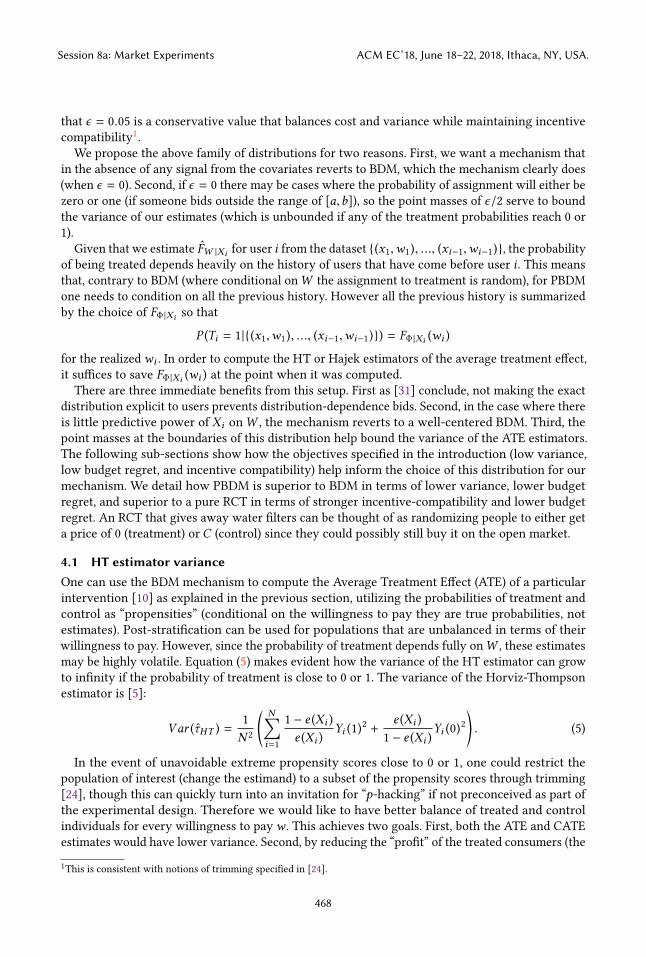
One can use the BDM mechanism to compute the Average Treatment Efect (ATE) of a particularintervention [10] as explained in the previous section, utilizing the probabilities of treatment andcontrol as łpropensitiesž (conditional on the willingness to pay they are true probabilities, notestimates). Post-stratiication can be used for populations that are unbalanced in terms of theirwillingness to pay. However, since the probability of treatment depends fully onW , these estimatesmay be highly volatile. Equation (5) makes evident how the variance of the HT estimator can growto ininity if the probability of treatment is close to 0 or 1. The variance of the Horviz-Thompsonestimator is [5]:

Var (τHT ) =1

N 2*,

N∑

i=1

1 − e (Xi )

e (Xi )Yi (1)

2+

e (Xi )

1 − e (Xi )Yi (0)

2+- . (5)

In the event of unavoidable extreme propensity scores close to 0 or 1, one could restrict thepopulation of interest (change the estimand) to a subset of the propensity scores through trimming[24], though this can quickly turn into an invitation for łp-hackingž if not preconceived as part ofthe experimental design. Therefore we would like to have better balance of treated and controlindividuals for every willingness to payw . This achieves two goals. First, both the ATE and CATEestimates would have lower variance. Second, by reducing the łproitž of the treated consumers (the

1This is consistent with notions of trimming speciied in [24].


468

diference between their willingness to pay and the price they paid), researchers would have lessregret about their subsidy of the product as will be explained in more detail in the next subsection.

The Hajek estimator’s variance can be related to the HT variance. The standard approach here isto linearize the Hajek estimator around the HT estimator and then take the variance and truncatehigher order terms. We thus concentrate on the HT estimator for comparing variance acrossmechanisms; the results presented in this section apply for the Hajek estimator asymptotically2.How should we design the conditional price distribution, Φ|X , to balance the treatment and

control? The variance in equation (5) can be modiied by replacing the propensities with FΦ |X , the(true) probability of being treated by our personalized mechanism:

Var (τHT ) =1

N 2*,

N∑

i=1

1 − FΦ |Xi(Wi )

FΦ |Xi(Wi )

Yi (1)2+

FΦ |Xi(Wi )

1 − FΦ |Xi(Wi )

Yi (0)2+- . (6)

Under a (rather strong) null hypothesis of no individual treatment efect (Fisher’s null, see [15])where Yi (1) − Yi (0) = 0 ∀i , meaning Yi (1) = Yi (0) = αi , we can write the variance as:

Var (τHT ) =1

N 2

N∑

i=1

αi

(

1 − FΦ |Xi(Wi )

FΦ |Xi(Wi )

+

FΦ |Xi(Wi )

1 − FΦ |Xi(Wi )

)

. (7)

This expression is minimized when FΦ |Xi(Wi ) =

12 for allWi , for any realization ofw1, ...,wN . If

we are only interested in minimizing Var (τHT ) under the null, there is a simple solution: we canjust place half of the probability mass of Φ on 0 and the other half on the upper bound forWi . Thisprovides an intuition for why randomized control trials are the gold standard for estimating causalefects. Yet, our objective is not only the estimation of an ATE: we are also interested in estimatingthe demand for the product and reducing the regret over our spent budget. Deploying an RCTactually achieves the upper bound for the budget regret (for any subject treated, they would pay 0and we would lose the full value of the product, C). With respect to estimating the demand, RCTsprovide no incentive to users for revealing their true willingness to pay, making the mechanismonly weakly incentive compatible.

Guaranteeing minimum variance for any realization ofW is a very strong condition. We insteadfocus on the expected variance, conditional on the observed characteristics Xi , with the expectationbeing taken over realizations ofW1, ...,WN . Using a Taylor expansion of Equation (6) around themean and taking a irst degree approximation, we then are interested in minimizing:

E[Var (τHT ) |X1, ...XN ] ≈1

N 2

N∑

i=1

(

1 − FΦ |Xi(E[Wi |Xi ])

FΦ |Xi(E[Wi |Xi ])

Yi (1)2+

FΦ |Xi(E[Wi |Xi ])

1 − FΦ |Xi(E[Wi |Xi ])

Yi (0)2

)

. (8)

Again assuming the Fisher null of no individual efect, this expected variance is minimized wheneverFΦ |Xi

(E[Wi |Xi ]) =12 , meaning that the median from the price distribution thus needs to be equal

to the conditional expectation of the willingness to pay distribution.One of the biggest advantages of PBDM over BDM is that it łsmoothsž the probability of a unit

to be treated or controlled, depending on the distribution ofW |Xi . This is, if the distribution ofW |Xi is skewed to the right, where users would be rarely treated, PBDM would łfocusž in this partof the distribution and would increase the probability of treatment. On the other hand ifW |Xi isskewed to the left then PBDM could diminish the probability of łhigh spendersž to be treated. Ourobjective however is clearly underspeciied in that there is an ininite number of distributions thatachieve this goal. We can therefore target additional goals within this space of distributions.

2See [37], pages 172ś176.


469

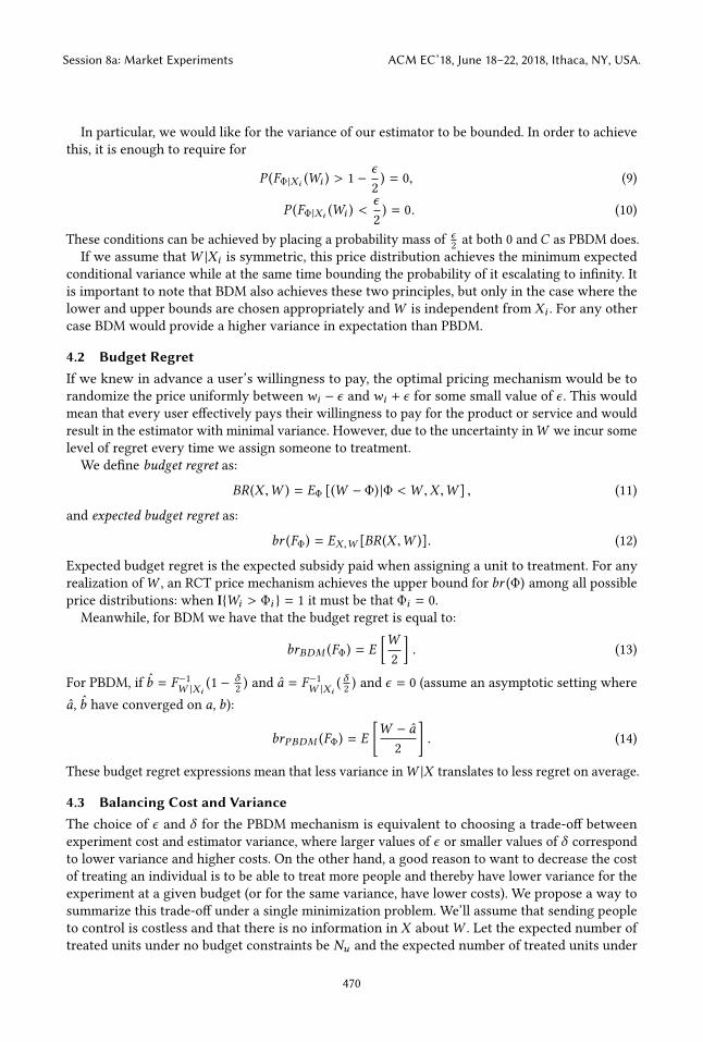
In particular, we would like for the variance of our estimator to be bounded. In order to achievethis, it is enough to require for

P (FΦ |Xi(Wi ) > 1 −

ϵ

2) = 0, (9)

P (FΦ |Xi(Wi ) <

ϵ

2) = 0. (10)

These conditions can be achieved by placing a probability mass of ϵ2 at both 0 andC as PBDM does.

If we assume thatW |Xi is symmetric, this price distribution achieves the minimum expectedconditional variance while at the same time bounding the probability of it escalating to ininity. Itis important to note that BDM also achieves these two principles, but only in the case where thelower and upper bounds are chosen appropriately andW is independent from Xi . For any othercase BDM would provide a higher variance in expectation than PBDM.

4.2 Budget Regret

If we knew in advance a user’s willingness to pay, the optimal pricing mechanism would be torandomize the price uniformly betweenwi − ϵ andwi + ϵ for some small value of ϵ . This wouldmean that every user efectively pays their willingness to pay for the product or service and wouldresult in the estimator with minimal variance. However, due to the uncertainty inW we incur somelevel of regret every time we assign someone to treatment.We deine budget regret as:

BR (X ,W ) = EΦ [(W − Φ) |Φ <W ,X ,W ] , (11)

and expected budget regret as:

br (FΦ) = EX ,W [BR (X ,W )]. (12)

Expected budget regret is the expected subsidy paid when assigning a unit to treatment. For anyrealization ofW , an RCT price mechanism achieves the upper bound for br (Φ) among all possibleprice distributions: when I{Wi > Φi } = 1 it must be that Φi = 0.Meanwhile, for BDM we have that the budget regret is equal to:

brBDM (FΦ) = E

[W

2

]. (13)

For PBDM, if b = F−1W |Xi

(1 − δ2 ) and a = F−1

W |Xi( δ2 ) and ϵ = 0 (assume an asymptotic setting where

a, b have converged on a, b):

brPBDM (FΦ) = E

[W − a

2

]. (14)

These budget regret expressions mean that less variance inW |X translates to less regret on average.

4.3 Balancing Cost and Variance

The choice of ϵ and δ for the PBDM mechanism is equivalent to choosing a trade-of betweenexperiment cost and estimator variance, where larger values of ϵ or smaller values of δ correspondto lower variance and higher costs. On the other hand, a good reason to want to decrease the costof treating an individual is to be able to treat more people and thereby have lower variance for theexperiment at a given budget (or for the same variance, have lower costs). We propose a way tosummarize this trade-of under a single minimization problem. We’ll assume that sending peopleto control is costless and that there is no information in X aboutW . Let the expected number oftreated units under no budget constraints be Nu and the expected number of treated units under


470

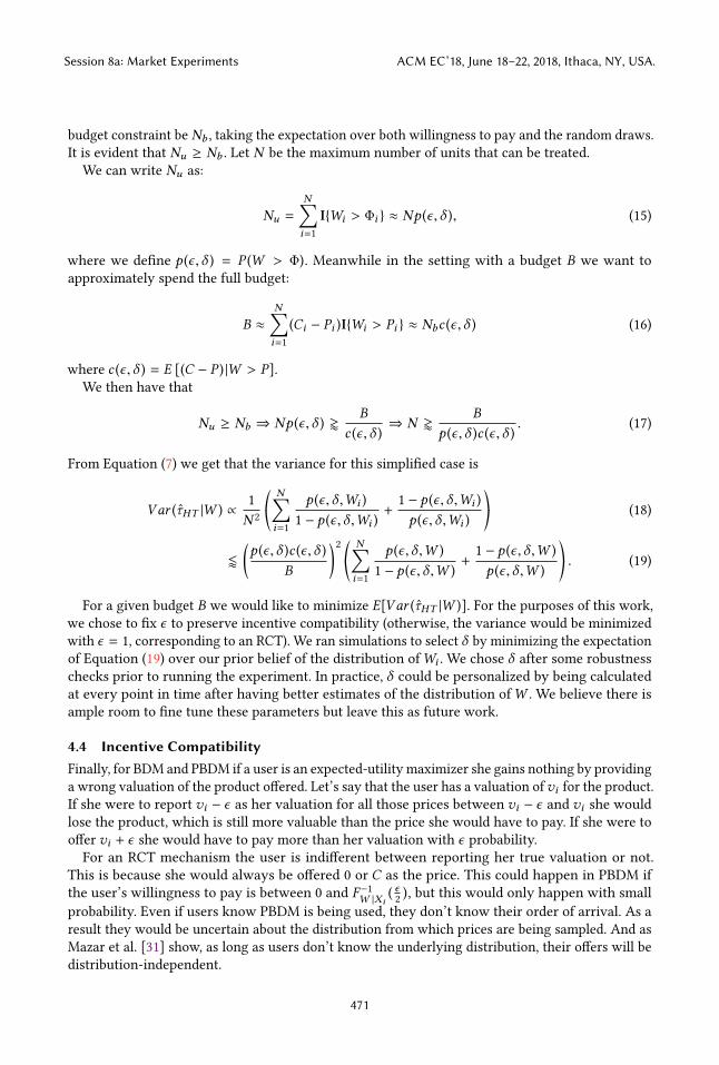
budget constraint be Nb , taking the expectation over both willingness to pay and the random draws.It is evident that Nu ≥ Nb . Let N be the maximum number of units that can be treated.

We can write Nu as:

Nu =

N∑

i=1

I{Wi > Φi } ≈ Np (ϵ,δ ), (15)

where we deine p (ϵ,δ ) = P (W > Φ). Meanwhile in the setting with a budget B we want toapproximately spend the full budget:

B ≈

N∑

i=1

(Ci − Pi )I{Wi > Pi } ≈ Nbc (ϵ,δ ) (16)

where c (ϵ,δ ) = E [(C − P ) |W > P].We then have that

Nu ≥ Nb ⇒ Np (ϵ,δ ) ⪆B

c (ϵ,δ )⇒ N ⪆

B

p (ϵ,δ )c (ϵ,δ ). (17)

From Equation (7) we get that the variance for this simpliied case is

Var (τHT |W ) ∝1

N 2*,

N∑

i=1

p (ϵ,δ ,Wi )

1 − p (ϵ,δ ,Wi )+

1 − p (ϵ,δ ,Wi )

p (ϵ,δ ,Wi )+- (18)

⪅

(

p (ϵ,δ )c (ϵ,δ )

B

)2 *,N∑

i=1

p (ϵ,δ ,W )

1 − p (ϵ,δ ,W )+

1 − p (ϵ,δ ,W )

p (ϵ,δ ,W )+- . (19)

For a given budget B we would like to minimize E[Var (τHT |W )]. For the purposes of this work,we chose to ix ϵ to preserve incentive compatibility (otherwise, the variance would be minimizedwith ϵ = 1, corresponding to an RCT). We ran simulations to select δ by minimizing the expectationof Equation (19) over our prior belief of the distribution ofWi . We chose δ after some robustnesschecks prior to running the experiment. In practice, δ could be personalized by being calculatedat every point in time after having better estimates of the distribution ofW . We believe there isample room to ine tune these parameters but leave this as future work.

4.4 Incentive Compatibility

Finally, for BDM and PBDM if a user is an expected-utility maximizer she gains nothing by providinga wrong valuation of the product ofered. Let’s say that the user has a valuation ofvi for the product.If she were to report vi − ϵ as her valuation for all those prices between vi − ϵ and vi she wouldlose the product, which is still more valuable than the price she would have to pay. If she were toofer vi + ϵ she would have to pay more than her valuation with ϵ probability.For an RCT mechanism the user is indiferent between reporting her true valuation or not.

This is because she would always be ofered 0 or C as the price. This could happen in PBDM ifthe user’s willingness to pay is between 0 and F−1

W |Xi( ϵ2 ), but this would only happen with small

probability. Even if users know PBDM is being used, they don’t know their order of arrival. As aresult they would be uncertain about the distribution from which prices are being sampled. And asMazar et al. [31] show, as long as users don’t know the underlying distribution, their ofers will bedistribution-independent.


471

4.5 Why not use the predicted median as the price?

We have thus far described a personalized mechanism that outperforms BDM in all of the describeddimensions. One may ask however why not just predict the medianWi |Xi and use this as theofered price. This was actually the original mechanism we envisioned for this problem, running asimple median regression onWi |Xi . If the covariates are highly predictive ofWi we would achievea 50-50 split and achieve close to minimum budget regret. However, we would not be able toassume thatWi is ixed (but previously unknown) for every user, since doing so would make theprobability of being assigned to treatment conditional onWi either 0 or 1, losing randomness inthe conditional assignment and breaking the assumption that treatment needs to be assigned atrandom in order to make causal interpretations. Even if we assumed that the randomness comesfrom some probabilistic process in how people elicit their willingness to pay, one could have anunobserved variable correlated with both the willingness to pay and the outcome which wouldcomplicate causal interpretations.

5 EMAIL CLASSIFICATION MOCK EXPERIMENT

In order to test our method we designed a Mechanical Turk task where users performed emailspam classiication [17]. After performing several rounds of classiication, the users were oferedthe opportunity to spend part of their wages in order to forgo a time restriction on their work.The time restriction made the task signiicantly more diicult, and they experienced the task bothwith and without the time restriction before being ofered the opportunity to remove it. The oferto pay to remove the restriction was formulated as a willingness to pay experiment. Users wererandomly assigned to either the standard BDM mechanism or our PBDM mechanism. The objectivein this mock experiment was thus to estimate both the demand for time freedom (the willingnessto pay for it) and the causal efect of being time-restricted on performance (better or worse spamclassiication).We conducted our experiment on Amazon Mechanical Turk for its convenience and simplicity

for running experiments. Mechanical Turk compares favorably to traditional ways of conductingbehavioral experiments [13]; see [30, 35] for discussions of best practices for behavioral researchusing Mechanical Turk.

We collected a range of covariates as the basis for our personalization under the PBDMmechanism.First, our task was hosted on a server that allowed us to gather browser-level features of the webusers. Second, we included two surveys at the onset of the task: a demographic survey in order tocompare our population with that of Mechanical Turk [25] and a risk survey, adapted from [18].For computing the risk proile of users from this survey we used the index for general risk aversionas in [29]. Lastly, we also collected additional covariates from the behavior of users during the earlytutorial phase of our task.

The users were not made aware that their browser coniguration or survey responses impactedthe phantom bidder of the PBDM mechanism. We had no true way of verifying the validity of thedemographic survey responses or the risk survey responses, and it is important to be clear thatthese responses ultimately impacted the price at which these users were ofered the time freedom.As a result, in settings where the subject may realize the connection between their responses toearly questions and the price ofered in a later stage of an experiment, it may be appropriate to onlyuse survey questions for which answers can be validated. Examples of questions from developmenteconomics ield experiments used in similar contexts include łHow many members are there inyour household?ž or łHow many rooms do you have in your home?ž [2]. Note, however, that evenif the users are able to impact their ofer distribution in their favor, it is still in their interest tobid their true willingness to pay, regardless of how much they’ve been able to manipulate the


472

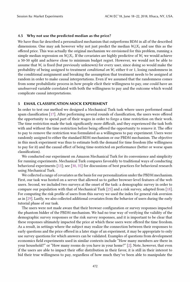
BDM PBDM

Number of participants 71 71

Percentage treated 31% 52%

Total cost (credits) 5469 6146

Cost per person treated (credits) 237 161

Average budget regret 65 45

HT ATE-0.63 12.09

(-38,36) (2.09,22.09)

Hajek ATE2.23 4.26

(-4.55,9.03) (2.78,5.73)

Block ATE5.19 3.8

(3.56,6.81) (1.91,5.70)

Table 1. PBDM improves on BDM in terms of cost per person, budget regret, and variance of the average

treatment efect estimators.

prediction algorithms such as Gradient Boosting Decision Trees, Adaboost, and Lasso post-fact3.We observe that none of these algorithms did a good job of predicting the personalized willingnessto pay from the covariates we gathered for our mock application, with all the models revertingto the population mean to predictW . This highlights an important basic beneit of PBDM: for allBDM experiments there is a basic population-level personalization problem of what the populationof responses will look like. A PBDM mechanism that simply learns the population of bids withreasonable idelity therefore delivers signiicant improvements over BDM, as our results show.Figure 2 shows the estimated intervals as well as the PBDM phantom bid for every user.

6 RESULTS

We use the email classiication task in the previous section to evaluate our PBDM mechanism incontrast with an ordinary BDM mechanism. Our evaluation is ive fold: we examine the cost ofrunning our experiment, the cost per person treated, the variance of the average treatment efect(ATE) estimators, the CATE conditional onW , and the expected budget regret. Table 1 summarizesthese diferences. For costs, the credits we pay to user i is 10 times the diference between thenumber of correct answers, Yi , and the number of incorrect answers (out of 20), 20 − Yi , minus theamount paid in case of treatment: 10(Yi − (20 − Yi )) − Φi I{Wi > Φi }.

For the variance of the average treatment efect estimators, we focus on the variance of theHorvitz-Thompson estimator and the consistent estimator of this variance [4]:

V ar (τHT ) =1

N 2*,

N∑

i=1

Ti (1 − e (Xi ))

[Yi (1)

e (Xi )

]2+ (1 −Ti ) (e (Xi ))

[Yi (0)

1 − e (Xi )

]2+- . (20)

Here e (Xi ) is the probability of assignment to treatment, which we can compute exactly giventhe known distribution of Φi |Xi at every stage of the experiment. As detailed in Section 4.1, wecan obtain Hajek variances estimates from HT variance estimates by linearization and Taylor

expansion to obtain V ar (τHajek). We use this estimate V ar (τHajek) to construct conservative Wald-

type conidence intervals for the ATE, τHajek ± z1−α

√

V ar (τHajek). Furthermore, we build bootstrap

conidence intervals for V ar (τHajek) under Fisher’s null (no individual treatment efect [15]). We

3In practice, researchers can run a variety of prediction algorithms at runtime (rather than post-fact) and make predictions

with the one with the best performance under a pre-speciied metric.


475

of the estimate. As a more advanced matter, we designed our PBDM mechanism to be able totailor the mechanism to the known covariates of each individual, learningW |Xi . That said, in ourpractical demonstration using a spam labelling task, we found that no covariates that we collectedwere able to meaningfully predict individual willingnesses to pay.

In terms of personalization, we believe there are further improvements to be made. Recentwork in the estimation of conidence intervals for machine learning techniques (see [7] wouldallow more sophisticated algorithms to be used as predictors ofW ’s distribution. Furthermore, amore sophisticated characterization of the phantom bidder distribution could yield better resultsin contexts where the distributional properties of the demand may be known a priori, as in wellestablished markets.Even with the simple representation of the phantom bidder used in this work we have high

conidence that a personalized BDMmechanism can result in substantial savings in experimentationcosts as well as improvements in statistical eiciency for a broad class of willingness to payexperiments.

REFERENCES

[1] Alekh Agarwal, Sarah Bird, Markus Cozowicz, Luong Hoang, John Langford, Stephen Lee, Jiaji Li, Dan Melamed, Gal

Oshri, Oswaldo Ribas, Siddhartha Sen, and Alex Slivkins. 2016. Making Contextual Decisions with Low Technical

Debt. arXiv preprint arXiv:1606.03966 (2016).

[2] Vivi Alatas, Ririn Purnamasari, Matthew Wai-Poi, Abhijit Banerjee, Benjamin A Olken, and Rema Hanna. 2016.

Self-targeting: Evidence from a ield experiment in Indonesia. Journal of Political Economy 124, 2 (2016), 371ś427.

[3] Joshua D Angrist and Jörn-Stefen Pischke. 2008. Mostly harmless econometrics: An empiricist’s companion. Princeton

University Press.

[4] Peter M Aronow. 2016. Data-Adaptive Causal Efects and Supereiciency. Journal of Causal Inference 4, 2 (2016).

[5] Peter M Aronow and Cyrus Samii. 2017. Estimating average causal efects under general interference, with application

to a social network experiment. The Annals of Applied Statistics 11, 4 (2017), 1912ś1947.

[6] Nava Ashraf, James Berry, and Jesse M Shapiro. 2010. Can higher prices stimulate product use? Evidence from a ield

experiment in Zambia. American Economic Review 100, 5 (2010), 2383ś2413.

[7] Susan Athey and Guido Imbens. 2016. Recursive partitioning for heterogeneous causal efects. Proceedings of the

National Academy of Sciences 113, 27 (2016), 7353ś7360.

[8] Hamsa Bastani, Mohsen Bayati, and Khashayar Khosravi. 2017. Exploiting the Natural Exploration In Contextual

Bandits. arXiv preprint arXiv:1704.09011 (2017).

[9] Gordon M Becker, Morris H DeGroot, and Jacob Marschak. 1964. Measuring utility by a single-response sequential

method. Behavioral science 9, 3 (1964), 226ś232.

[10] James Berry, Greg Fischer, and Raymond P Guiteras. 2015. Eliciting and utilizing willingness to pay: evidence from

ield trials in Northern Ghana. (2015).

[11] Peter Bohm, Johan Lindén, and Joakim Sonnegård. 1997. Eliciting reservation prices: BeckerśDeGrootśMarschak

mechanisms vs. markets. The Economic Journal 107, 443 (1997), 1079ś1089.

[12] Rebecca R Boyce, Thomas C Brown, Gary H McClelland, George L Peterson, and William D Schulze. 1992. An

experimental examination of intrinsic values as a source of the WTA-WTP disparity. The American Economic Review

82, 5 (1992), 1366ś1373.

[13] Michael Buhrmester, Tracy Kwang, and Samuel D Gosling. 2011. Amazon’s Mechanical Turk a new source of

inexpensive, yet high-quality, data? Perspectives on psychological science 6, 1 (2011), 3ś5.

[14] Bob Carpenter, Andrew Gelman, Matt Hofman, Daniel Lee, Ben Goodrich, Michael Betancourt, Michael A Brubaker,

Jiqiang Guo, Peter Li, and Allen Riddell. 2016. Stan: A probabilistic programming language. Journal of Statistical

Software 20, 2 (2016), 1ś37.

[15] Peng Ding. 2017. A paradox from randomization-based causal inference. Statistical science 32, 3 (2017), 331ś345.

[16] Ronald A Fisher. 1937. The design of experiments. Oliver And Boyd; Edinburgh; London.

[17] Daniel G Goldstein, Siddharth Suri, R Preston McAfee, Matthew Ekstrand-Abueg, and Fernando Diaz. 2014. The

economic and cognitive costs of annoying display advertisements. Journal of Marketing Research 51, 6 (2014), 742ś752.

[18] Ramu Govindasamy and John Italia. 1999. Predicting willingness-to-pay a premium for organically grown fresh

produce. Journal of Food Distribution Research 30 (1999), 44ś53.

[19] David M Grether and Charles R Plott. 1979. Economic theory of choice and the preference reversal phenomenon. The

American Economic Review 69, 4 (1979), 623ś638.


479

[20] Jaroslav Hájek. 1971. Comment on łAn essay on the logical foundations of survey sampling, part onež. The foundations

of survey sampling 236 (1971).

[21] Jason Hartford, Greg Lewis, Kevin Leyton-Brown, and Matt Taddy. 2016. Counterfactual Prediction with Deep

Instrumental Variables Networks. arXiv preprint arXiv:1612.09596 (2016).

[22] Daniel G Horvitz and Donovan J Thompson. 1952. A generalization of sampling without replacement from a inite

universe. Journal of the American statistical Association 47, 260 (1952), 663ś685.

[23] Taisuke Imai and Colin F Camerer. 2016. Estimating Time Preferences from Budget Set Choices Using Optimal Adaptive

Design. Working Paper (2016).

[24] Guido W Imbens and Donald B Rubin. 2015. Causal inference in statistics, social, and biomedical sciences. Cambridge

University Press.

[25] Panagiotis G Ipeirotis. 2010. Demographics of mechanical turk. (2010).

[26] Steven J Kachelmeier and Mohamed Shehata. 1992. Examining risk preferences under high monetary incentives:

Experimental evidence from the People’s Republic of China. The American Economic Review (1992), 1120ś1141.

[27] Dean Karlan and Jonathan Zinman. 2009. Observing unobservables: Identifying information asymmetries with a

consumer credit ield experiment. Econometrica 77, 6 (2009), 1993ś2008.

[28] Lihong Li, Wei Chu, John Langford, and Robert E Schapire. 2010. A contextual-bandit approach to personalized news

article recommendation. In Proceedings of the 19th international conference on World wide web. ACM, 661ś670.

[29] Carter AMandrik and Yeqing Bao. 2005. Exploring the concept and measurement of general risk aversion. NA-Advances

in Consumer Research Volume 32 (2005).

[30] Winter Mason and Siddharth Suri. 2012. Conducting behavioral research on Amazon’s Mechanical Turk. Behavior

research methods 44, 1 (2012), 1ś23.

[31] Nina Mazar, Botond Koszegi, and Dan Ariely. 2014. True context-dependent preferences? The causes of market-

dependent valuations. Journal of Behavioral Decision Making 27, 3 (2014), 200ś208.

[32] Timothy L McMurry and Dimitris N Politis. 2008. Bootstrap conidence intervals in nonparametric regression with

built-in bias correction. Statistics & Probability Letters 78, 15 (2008), 2463ś2469.

[33] Jerzey Neyman. 1923. On the application of probability theory to agricultural experiments. Essay on principles. Section

9. Edited and translated by DM Dabrowska and TP Speed. Statist. Sci. 5 (1923), 465ś72.

[34] Charles Noussair, Stephane Robin, and Bernard Ruieux. 2004. Revealing consumers’ willingness-to-pay: A comparison

of the BDM mechanism and the Vickrey auction. Journal of economic psychology 25, 6 (2004), 725ś741.

[35] Gabriele Paolacci, Jesse Chandler, and Panagiotis G Ipeirotis. 2010. Running experiments on amazon mechanical turk.

(2010).

[36] Donald B Rubin. 1974. Estimating causal efects of treatments in randomized and nonrandomized studies. Journal of

educational Psychology 66, 5 (1974), 688.

[37] Carl-Erik Särndal, Bengt Swensson, and Jan Wretman. 1992. Model assisted survey sampling. Springer Science &

Business Media.

[38] Adith Swaminathan and Thorsten Joachims. 2015. The self-normalized estimator for counterfactual learning. In

Advances in Neural Information Processing Systems. 3231ś3239.

[39] Stefan Wager and Susan Athey. 2017. Estimation and inference of heterogeneous treatment efects using random

forests. J. Amer. Statist. Assoc. just-accepted (2017).

[40] Nathaniel T Wilcox. 1993. On a lottery pricing anomaly: time tells the tale. Journal of Risk and Uncertainty 7, 3 (1993),

311ś324.


480

a personalized bdm mechanism for efficient market

Documents