J Glob Optim (2007) 39:197–219DOI 10.1007/s10898-007-9133-5

O R I G I NA L PA P E R

A particle swarm pattern search method for boundconstrained global optimization

A. Ismael F. Vaz · Luís N. Vicente

Received: 12 February 2006 / Accepted: 3 January 2007 / Published online: 6 February 2007© Springer Science+Business Media B.V. 2007

Abstract In this paper we develop, analyze, and test a new algorithm for the globalminimization of a function subject to simple bounds without the use of derivatives.The underlying algorithm is a pattern search method, more specifically a coordinatesearch method, which guarantees convergence to stationary points from arbitrarystarting points. In the optional search phase of pattern search we apply a particleswarm scheme to globally explore the possible nonconvexity of the objective func-tion. Our extensive numerical experiments showed that the resulting algorithm ishighly competitive with other global optimization methods also based on functionvalues.

Keywords Direct search · Pattern search · Particle swarm · Derivative free optimi-zation · Global optimization · Bound constrained nonlinear optimization

AMS subject classifications 90C26 · 90C30 · 90C56

Support for A. Ismael F. Vaz was provided by Algoritmi Research Center, and by FCT under grantsPOCI/MAT/59442/2004 and POCI/MAT/58957/2004.Support for Luís N. Vicente was provided by Centro de Matemática da Universidade de Coimbraand by FCT under grant POCI/MAT/59442/2004.

A. I. F. Vaz (B)Departamento de Produção e Sistemas, Escola de Engenharia,Universidade do Minho,Campus de Gualtar, 4710-057 Braga, Portugale-mail: aivaz@dps.uminho.pt

L. N. VicenteDepartamento de Matemática,Universidade de Coimbra,3001-454 Coimbra, Portugale-mail: lnv@mat.uc.pt

198 J Glob Optim (2007) 39:197–219

1 Introduction

Pattern and direct search methods are one of the most popular classes of methodsto minimize functions without the use of derivatives or of approximations to deriva-tives [26]. They are based on generating search directions which positively span thesearch space. Direct search is conceptually simple and natural for parallelization.These methods can be designed to rigorously identify points satisfying stationarityfor local minimization (from arbitrary starting points). Moreover, their flexibility canbe used to incorporate algorithms or heuristics for global optimization, in a way thatthe resulting direct or pattern search method inherits some of the properties of theimported global optimization technique, without jeopardizing the convergence forlocal stationarity mentioned before.

The particle swarm optimization algorithm was firstly proposed in ref. [12,24] andhas received some recent attention in the global optimization community [7,35]. Theparticle swarm algorithm tries to simulate the social behavior of a population of agentsor particles, in an attempt to optimally explore some given problem space. At a timeinstant (an iteration in the optimization context), each particle is associated with astochastic velocity vector which indicates where the particle is moving to. The velocityvector for a given particle at a given time is a linear stochastic combination of thevelocity in the previous time instant, of the direction to the particle’s best position,and of the direction to the best swarm positions (for all particles). The particle swarmalgorithm is a stochastic algorithm in the sense that it relies on parameters drawn fromrandom variables, and thus different runs for the same starting swarm may producedifferent outputs. Some of its advantages are being simple to implement and easy toparallelize. It depends, however, on a few of parameters which influence the rate ofconvergence in the vicinity of the global optimum. Overall it does not require manyuser-defined parameters, which is important for practitioners that are not familiar withoptimization. Some numerical evidence seems to show that particle swarm can outper-form genetic algorithms on difficult problem classes, namely for unconstrained globaloptimization problems [6]. Moreover, it fits nicely into the pattern search framework.

The goal of this paper is to show how particle swarm can be incorporated in thepattern search framework. The resulting particle swarm pattern search algorithm isstill a pattern search algorithm, producing sequences of iterates along the traditionalrequirements for this class of methods (based on integer lattices and positive span-ning sets). The new algorithm is better equipped for global optimization because itis more aggressive in the exploration of the search space. Our numerical experiencesshowed that a large percentage of the computational work is spent in the particleswarm component of pattern search.

Within the pattern search framework, the use of the search step for surrogateoptimization [5,30] or global optimization [1] is an active area of research. Hart hasalso used evolutionary programming to design evolutionary pattern search methods(see [16] and the references therein). There are some significative differences betweenhis work and ours. First, we are exclusively focused on global optimization and ourheuristic is based on particle swarm rather than on evolutionary algorithms. Further,our algorithm is deterministic in its pattern search component. As a result, we obtainthat a subsequence of the mesh size parameters tends to zero in the deterministicsense rather than with probability one like in Hart’s algorithms.

J Glob Optim (2007) 39:197–219 199

We are interested in solving optimization problems of the form

minz∈Rn

f (z) s.t. z ∈ �

with� = {

z ∈ Rn : � ≤ z ≤ u

},

where the inequalities � ≤ z ≤ u are posed componentwise and � ∈ (−∞, R)n,u ∈ (R, +∞)n, and � < u. There is no need to assume any type on smoothness on theobjective function f (z) to apply particle swarm or pattern search. To study the con-vergence properties of pattern search, and thus of the particle swarm pattern searchmethod, one has to impose some smoothness on f (z), in particular to characterizestationarity at local minimizers.

The next two sections are used to describe the particle swarm paradigm and thebasic pattern search framework. We introduce the particle swarm pattern searchmethod in Sect. 4. The convergence and termination properties of the proposedmethod are discussed in Sect. 5. A brief review about the optimization solvers used inthe numerical comparisons and implementation details about our method are givenin Sect. 6. The numerical results are presented in Sect. 7 for a large set of problems.We end the paper in Sect. 8 with conclusions and directions for future work.

2 Particle swarm

In this section, we briefly describe the particle swarm optimization algorithm. Ourdescription follows the presentation of the algorithm tested in ref. [6] and the readeris pointed to ref. [6] for other algorithmic variants and details.

The particle swarm optimization algorithm is based on a population (swarm) of sparticles, where s is known as the population size. Each particle is associated with avelocity which indicates where the particle is moving to. Let t be a time instant. Thenew position xi(t + 1) of the ith particle at time t + 1 is computed by adding to the oldposition xi(t) at time t a velocity vector vi(t + 1):

xi(t + 1) = xi(t) + vi(t + 1) (1)

for i = 1, . . . , s.The velocity vector associated to each particle i is updated by

vij(t + 1) = ι(t)vi

j(t) + µω1j(t)(

yij(t) − xi

j(t))

+ νω2j(t)(

yj(t) − xij(t)

)(2)

for j = 1, . . . , n, where ι(t) is a weighting factor (called inertial) and µ and ν are positivereal parameters (called, in the particle swarm terminology, the cognition parameterand the social parameter, respectively). The numbers ω1j(t) and ω2j(t), j = 1, . . . , n,are randomly drawn from the uniform (0, 1) distribution. Finally, yi(t) is the positionof the ith particle with the best objective function value so far calculated, and y(t)is the particle position with the best (among all particles) objective function valuefound so far. The update formula (2) adds to the previous velocity vector a stochasticcombination of the directions to the best position of the ith particle and to the best(among all) particles position.

The position y(t) can be described as

y(t) ∈ argminz∈{y1(t),...,ys(t)}f (z).

200 J Glob Optim (2007) 39:197–219

The argmin operator can return a set. When that happens in this situation, it is the firstelement in this argmin set that matches the implementations, since the best elementis only updated algorithmically when a new one is found yielding a decrease in theobjective function.

The bound constraints in the variables are enforced by considering the projectiononto �, given for all particles i = 1, . . . , s by

proj�(xij(t)) =

⎧⎪⎨

⎪⎩

�j, if xij(t) < �j,

uj, if xij(t) > uj,

xij(t), otherwise

(3)

for j = 1, . . . , n. This projection must be applied to the new particles positions com-puted by Eq. (1).

The stopping criterion of the algorithm should be practical and has to ensure propertermination. One possibility is to stop when the norm of the velocities vector is smallfor all particles. It is possible to prove under some assumptions and for some algorith-mic parameters that the expected value of the norm of the velocities vectors tends tozero for all particles (see also the analysis presented in Sect. 5).

The particle swarm optimization algorithm is described in Algorithm 2.1.

Algorithm 2.1

1. Choose a population size s and a stopping tolerance vtol > 0. Randomly ini-tialize the initial swarm positions x1(0), . . . , xs(0) and the initial swarm velocitiesv1(0), . . . , vs(0).

2. Set yi(0) = xi(0), i = 1, . . . , s, and y(0) ∈ arg minz∈{y1(0),...,ys(0)} f (z). Let t = 0.3. Set y(t + 1) = y(t).

For i = 1, . . . , s do (for every particle i):• Compute xi(t) = proj�(xi(t)).• If f (xi(t)) < f (yi(t)) then

(a) Set yi(t + 1) = xi(t) (update the particle i best position).(b) If f (yi(t + 1)) < f (y(t + 1)) then y(t + 1) = yi(t + 1) (update the particles

best position).• Otherwise set yi(t + 1) = yi(t).

4. Compute vi(t + 1) and xi(t + 1), i = 1, . . . , s, using formulae (1) and (2).5. If ‖vi(t + 1)‖ < vtol, for all i = 1, . . . , s, then stop. Otherwise, increment t by one

and go to Step 3.

3 Pattern search

Direct search methods are an important class of optimization algorithms which at-tempt to minimize a function by comparing, at each iteration, its value in a finite setof trial points (computed by simple mechanisms). Direct search methods not only donot use any derivative information but also do not try to implicitly build any typeof derivative approximation. Pattern search methods can be seen as direct searchmethods for which the rules of generating the trial points follow stricter calculationsand for which convergence for stationary points can be proved from arbitrary startingpoints. A comprehensive review of direct and pattern search can be found in ref. [26],where a broader class of methods referred to as ‘generating set search’ is described.

J Glob Optim (2007) 39:197–219 201

In this paper, we prefer to describe pattern search methods using the search/poll stepframework [3], since it better suits the incorporation of heuristic procedures.

The central notion in pattern search are positive spanning sets. The definitions andproperties of positive spanning sets and of positive bases are given, for instance, inref. [10,26]. One of the simplest positive spanning sets is formed by the vectors of thecanonical basis and their negatives:

D⊕ = {e1, . . . , en, −e1, . . . , −en}.The set D⊕ is also a (maximal) positive basis. The elementary direct search methodbased on this positive spanning set is known as coordinate or compass search and itsstructure is basically all we need in this paper.

Given a positive spanning set D and the current iterate1 y(t), we define two sets ofpoints: the mesh Mt and the poll set Pt. The mesh Mt is given by

Mt ={

y(t) + α(t)Dz, z ∈ Z|D|+

},

where α(t) > 0 is the mesh size parameter (also known as the step-length controlparameter) and Z+ is the set of nonnegative integers. The mesh has to meet someintegrality requirements for the method to achieve global convergence to stationarypoints, in other words, convergence to stationary points from arbitrary starting points.In particular, the matrix D has to be of the form GZ, where G ∈ R

n×n is a nonsingulargenerating matrix and Z ∈ Z

n×|D|. The positive basis D⊕ satisfies this requirementtrivially when G is the identity matrix.

The search step conducts a finite search in the mesh Mt. The poll step is executedonly if the search step fails to find a point for which f is lower than f (y(t)). The pollstep evaluates the function at the points in the poll set

Pt = {y(t) + α(t)d, d ∈ D}trying to find a point where f is lower than f (y(t)). Note that Pt is a subset of Mt. If fis continuously differentiable at y(t), the poll step is guaranteed to succeed if α(t) issufficiently small, since the positive spanning set D contains at least one direction ofdescent (which makes an acute angle with −∇f (y(t))). Thus, if the poll step fails thenthe mesh size parameter must be reduced. It is the poll step that guarantees the globalconvergence of the pattern search method.

In order to generalize pattern search for bound constrained problems it is neces-sary to use a feasible initial guess y(0) ∈ � and to keep feasibility of the iterates byrejecting any trial point, that is, out of the feasible region. Rejecting infeasible trialpoints can be accomplished by applying a pattern search algorithm to the followingpenalty function

f (z) ={

f (z), if z ∈ �,+∞, otherwise.

The iterates produced by a pattern search method applied to the unconstrained prob-lem of minimizing f (z) coincide trivially with those generated by the same type ofpattern search method, but applied to the minimization of f (z) subject to simplebounds and to the rejection of infeasible trial points.

1 We will use y(t) to denote the current iterate, rather than xk or yk, to follow the notation of theparticle swarm framework.

202 J Glob Optim (2007) 39:197–219

It is also necessary to include in the search directions D those directions that guar-antee the presence of a feasible descent direction at any nonstationary point of thebound constrained problem. One can achieve this goal in several ways. But, sinceD⊕ includes all such directions [26], we assume the use of this set throughout theremainder of the paper.

In order to completely describe the basic pattern search algorithm, we need tospecify how to increase and decrease the mesh size or step-length control parameterα(t). These expansions and contractions use the factors φ(t) and θ(t), respectively,which must obey to the following rules:

φ(t) = τ �t , for some �t ∈ {0, . . . , �max}, if t is successful,θ(t) = τmt , for some mt ∈ {mmin, . . . , −1}, if t is unsuccessful,

where τ > 1 is a positive rational, �max is a nonnegative integer, and mmin is a negativeinteger, chosen at the beginning of the method and unchanged with t. For instance, wecan have θ(t) = 1/2 for unsuccessful iterations and φ(t) = 1 or φ(t) = 2 for successfuliterations.

The basic pattern search method for use in this paper is described in Algorithm 3.1.

Algorithm 3.1

1. Choose a positive rational τ and the stopping tolerance αtol > 0. Choose thepositive spanning set D = D⊕.

2. Let t = 0. Select an initial feasible guess y(0). Choose α(0) > 0.3. [Search Step]

Evaluate f at a finite number of points in Mt. If a point z(t) ∈ Mt is found forwhich f (z(t)) < f (y(t)) then set y(t + 1) = z(t), α(t + 1) = φ(t)α(t) (optionallyincreasing the mesh size parameter), and declare successful both the search stepand the current iteration.

4. [Poll Step]Skip the poll step if the search step was successful.• If there exists d(t) ∈ D such that f (y(t) + α(t)d(t)) < f (y(t)) then

(a) Set y(t + 1) = y(t) + α(t)d(t) (poll step and iteration successful).(b) Set α(t + 1) = φ(t)α(t) (optionally increase the mesh size parameter).

• Otherwise, f (y(t) + α(t)d(t)) ≥ f (y(t)) for all d(t) ∈ D, and(a) Set y(t + 1) = y(t) (iteration and poll step unsuccessful).(b) Set α(t + 1) = θ(t)α(t) (reduce the mesh size parameter).

5. If α(t + 1) < αtol then stop. Otherwise, increment t by one and go to Step 3.

An example of the use of the search step is given in the next section. The poll stepcan be implemented in a number of different ways. The polling can be opportunistic(when it quits once the first decrease in the objective function is found) or complete(when the objective function is evaluated at all the points of the poll set). The orderin which the points in Pt are evaluated can also differ [4,9].

4 The particle swarm pattern search method

Pattern search methods are local methods in the sense that they are designed toachieve convergence (from arbitrary starting points) to points that satisfy necessaryconditions for local optimality. Some numerical experience has shown cases in which

J Glob Optim (2007) 39:197–219 203

pattern search has found global minimizers for certain classes of problems (see, forinstance, [1,31]). Certain parameter choices can enable pattern search to jump out ofone basin of attraction of a local minimizer into another (that is hopefully a betterone). This paper is an attempt to exploit this tendency by applying a global heuristic inthe search step. On the other hand, the poll step can rigorously guarantee convergenceto stationary points.

The hybrid method introduced in this paper is a pattern search method that incor-porates a particle swarm search in the search step. The idea is to start with an initialpopulation and to apply one step of particle swarm at each search step. Consecutiveiterations where the search steps succeed reduce to consecutive iterations of particleswarm, in an attempt to identify a neighborhood of a global minimizer. Wheneverthe search step fails, the poll step is applied to the best position over all particles,performing a local search in the poll set centered at this point.

The points calculated in the search step by the particle swarm scheme must belongto the pattern search mesh Mt. This task can be done in several ways and, in particular,one can compute their ‘projection’ onto Mt

projMt(xi(t)) = min

u∈Mt‖u − xi(t)‖

for i = 1, . . . , s, or an approximation thereof.There is no need then to project onto � since the use of the penalty function f in

pattern search takes care of the bound constraints.The stopping criterion of the particle swarm pattern search method is the conjunc-

tion of the stopping criteria for particle swarm and pattern search. The particle swarmpattern search method is described in Algorithm 4.1.

Algorithm 4.1

1. Choose a positive rational τ and the stopping tolerance αtol > 0. Choose thepositive spanning set D = D⊕.Choose a population size s and a stopping tolerance vtol > 0. Randomly ini-tialize the initial swarm positions x1(0), . . . , xs(0) and the initial swarm velocitiesv1(0), . . . , vs(0).

2. Set yi(0) = xi(0), i = 1, . . . , s, and y(0) ∈ arg minz∈{y1(0),...,ys(0)} f (z). Choose α(0) >

0. Let t = 0.3. [Search Step]

Set y(t + 1) = y(t).For i = 1, . . . , s do (for every particle i):• Compute xi(t) = projMt

(xi(t)).

• If f (xi(t)) < f (yi(t)) then(a) Set yi(t + 1) = xi(t) (update the particle i best position).(b) If f (yi(t + 1)) < f (y(t + 1)) then

* Set y(t +1) = yi(t +1) (update the particles best position; search stepand iteration successful).

* Set α(t+1) = φ(t)α(t) (optionally increase the mesh size parameter).• Otherwise set yi(t + 1) = yi(t).

4. [Poll Step]Skip the poll step if the search step was successful.

• If there exists d(t) ∈ D such that f (y(t) + α(t)d(t)) < f (y(t)) then

204 J Glob Optim (2007) 39:197–219

(a) Set y(t + 1) = y(t) + α(t)d(t) (update the leader particle position; pollstep and iteration successful).

(b) Set α(t + 1) = φ(t)α(t) (optionally increase the mesh size parameter).• Otherwise, f (y(t) + α(t)d(t)) ≥ f (y(t)) for all d(t) ∈ D, and

(a) Set y(t + 1) = y(t) (no change in the leader particle position; poll stepand iteration unsuccessful).

(b) Set α(t + 1) = θ(t)α(t) (reduce the mesh size parameter).5. Compute vi(t + 1) and xi(t + 1), i = 1, . . . , s, using formulae (1) and (2).6. If α(t + 1) < αtol and ‖vi(t + 1)‖ < vtol, for all i = 1, . . . , s, then stop. Otherwise,

increment t by one and go to Step 3.

5 Convergence

The convergence analysis studies properties of a sequence of iterates generated byAlgorithm 4.1. For this purpose, we consider αtol = 0 and vtol = 0, so that the algo-rithm never meets the termination criterion. Let {y(t)} be the sequence of iteratesproduced by Algorithm 4.1. Since all necessary pattern search ingredients are pres-ent, this method generates, under the appropriate assumptions, a sequence of iteratesconverging (independently of the starting point) to first-order critical points. A stan-dard result for this class of methods tells us that there is a subsequence of unsuccessfuliterations converging to a limit point and for which the mesh size parameter tends tozero [3,26].

Theorem 5.1 Let L(y(0)) = {z ∈ Rn : f (z) ≤ f (y(0))} be a bounded set. Then, there

exists a subsequence {y(tk)} of the iterates produced by Algorithm 4.1 (with αtol = vtol =0) such that

limk−→+∞

y(tk) = y∗ and limk−→+∞

α(tk) = 0

for some y∗ ∈ � and such that the subsequence {tk} consists of unsuccessful iterations.

The integrality assumptions imposed in the construction of the meshes Mt and onthe update of the mesh size parameter are fundamental for the integer lattice typearguments required to prove this result. There are other ways to obtain such a resultthat circumvent the need for these integrality assumptions [26], such as the impositionof a sufficient decrease condition on the step acceptance mechanism.

Depending on the differentiability properties of the objective function, differenttypes of stationarity can be proved for the point y∗. For instance, if the function isstrictly differentiable at this point, one can prove from the positive spanning proper-ties of D that ∇f (y∗) = 0 (see [3]). A result of the type lim inf t−→+∞ ‖∇f (y(t))‖ = 0can only be guaranteed when f is continuously differentiable in L(y(0)) (see [26]).

Theorem 5.1 tells us that a stopping criterion based solely on the size of the meshsize parameter (of the form α(t) < αtol) will guarantee termination of the algorithmin a finite number of iterations. However, the stopping condition of Algorithm 4.1also requires ‖vi(t)‖ < vtol, i = 1, . . . , s (in an attempt to impose to particle swarm adesirable level of global optimization effort). Thus, it must be investigated whetheror not the velocities in the particle swarm scheme satisfy a limit of the form

limk−→+∞

‖vi(tk)‖ = 0, i = 1, . . . , s.

J Glob Optim (2007) 39:197–219 205

To do this we have to investigate the asymptotic behavior of the search step whichis where the particle swarm strategy is applied. Rigorously speaking such a limit canonly occur with probability one. To carry on the analysis we need to assume that xi(t),yi(t), vi(t), and y(t) are random variables of stochastic processes. Let E(·) denote theappropriate mean or expected value operator.

Theorem 5.2 Suppose that for t sufficiently large one has that ι(t), E(yi(t)), i = 1, . . . , s,and E(y(t)) are constant and that E(projMt

(xi(t − 1) + vi(t))) = E(xi(t − 1) + vi(t)),i = 1, . . . , s. Then, if the control parameters for particle swarm, ι, ω1, ω2, µ, and ν, arechosen so that max{|a|, |b|} < 1, where ω1 = E(ω1(t)), ω2 = E(ω2(t)), ι = ι(t) for all t,and a and b are defined, respectively, by (8) and (9), then

limt−→+∞ E(vi

j(t)) = 0, i = 1, . . . , s, j = 1, . . . , n

and Algorithm 4.1 will stop almost surely in a finite number of iterations.

Proof Given that there exists a subsequence driving the mesh size parameter to zero,it remains to investigate under what conditions do the velocities tend to zero.

Consider the velocity Eq. (2), repeated here for convenience, with the indices ifor the particles and j for the vector components dropped for simplicity. To shortennotation we write the indices t as subscripts. Since ω1(t) and ω2(t) depend only on t,we get from (2) that

E(vt+1) = ιE(vt) + µω1 (E(yt) − E(xt)) + νω2(E(yt) − E(xt)

), (4)

where ω1 = E(ω1(t)) and ω2 = E(ω2(t)). From (2), we obtain for v(t) that

E(vt) = ιE(vt−1) + µω1(E(yt−1) − E(xt−1)

)

+νω2(E(yt−1) − E(xt−1)

). (5)

Subtracting (5) from (4) yields

E(vt+1) − E(vt) = ι(E(vt) − E(vt−1)) − (µω1 + νω2)(E(xt) − E(xt−1))

+ µω1(E(yt) − E(yt−1)) + νω2(E(yt) − E(yt−1)).

Noting that xt = projMt(xt−1 + vt) we obtain the following inhomogeneous recur-

rence relation

E(vt+1) − (1 + ι − µω1 − νω2)E(vt) + ιE(vt−1) = gt, (6)

where

gt = µω1(E(yt) − E(yt−1)) + νω2(E(yt) − E(yt−1))

+ (µω1 + νω2)E(projMt(xt−1 + vt) − (xt−1 + vt)).

From the assumptions of the theorem, we have, for sufficiently large t, that gt iszero and therefore that the recurrence relation is homogeneous, with characteristicpolynomial given by

t2 − (1 + ι − µω1 − νω2)t + ι = 0. (7)

A solution of (6) is then of the form

E(vt+1) = c1at + c2bt,

206 J Glob Optim (2007) 39:197–219

where c1 and c2 are constants and a and b are the two roots of the characteristicpolynomial (7), given by

a = (1 + ι − µω1 − νω2) + √(1 + ι − µω1 − νω2)2 − 4ι

2, (8)

b = (1 + ι − µω1 − νω2) − √(1 + ι − µω1 − νω2)2 − 4ι

2. (9)

Thus, as long as max{|a|, |b|} < 1 (which is achievable for certain choices of the controlparameters ι, ω1, ω2, µ, and ν), we will get E(vt+1) → 0 when t → ∞. �

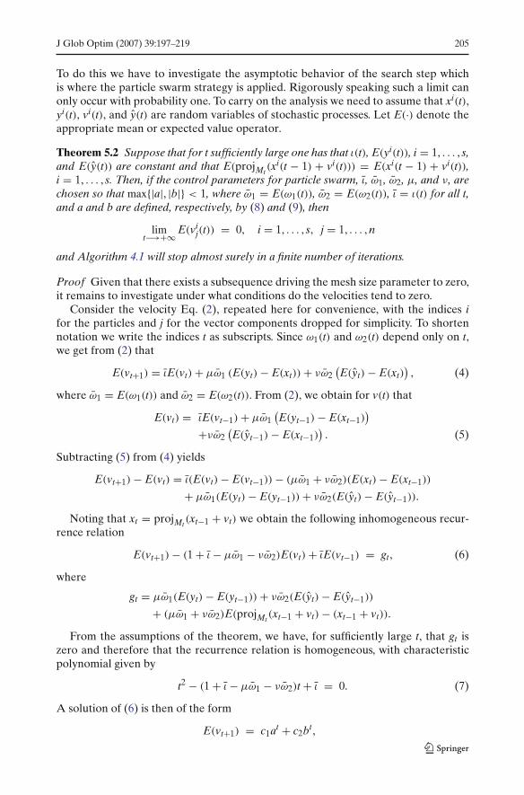
For instance, when ω1 = ω2 = 0.5 and µ = ν = 0.5, we obtain

a = (ι + 0.5) + √(ι + 0.5)2 − 4ι

2

and

b = (ι + 0.5) − √(ι + 0.5)2 − 4ι

2.

In this case, max{|a|, |b|} < 1 for any 0 < ι < 1. One can clearly observe this fact inFig. 1. Zooming into the picture reveals that for ι < 0.0858 we have (ι+0.5)2 −4ι ≥ 0,resulting in two real roots for the characteristic polynomial. For ι ≥ 0.0858 we havetwo complex conjugate roots whose moduli are equal.

It is difficult to show that the conditions of Theorem 5.2 can be rigorously satisfied,but it can be given some indication of their practical reasonability.

Given that the function is bounded below in L(y(0)), it is known that the monoton-ically decreasing sequences {f (yi(t))}, i = 1, . . . , s, and {f (y(t))} converge. Thus, it isreasonable to suppose that the expected values of yi(t), i = 1, . . . , s, and y(t) convergetoo.

On the other hand, the difference between projMt(xi(t − 1) + vi(t)) and xi(t−1)+

vi(t) — and thus between their expected values — is a multiple of α(t) for somechoices of D. This situation occurs in coordinate search, where D = D⊕. Since there isa subsequence of the mesh size parameters that converges to zero, there is at least theguarantee that the expected difference between xi(t − 1) + vi(t) and its projectiononto Mt converges to zero in that subsequence.

Fig. 1 Plot of ι forµω1 = νω2 = 0.25

0 0.1 0.2 0.3 0.4 0.5 0.6 0.7 0.8 0.9 10

0.1

0.2

0.3

0.4

0.5

0.6

0.7

0.8

0.9

1

ι

|a|,|

b|

|b|

|a|

|a|,|b|

J Glob Optim (2007) 39:197–219 207

So, there is at least some indication that the term gt in (6) converges to zerofor a subsequence of the iterates. Although this is not the same as saying that theassumptions of Theorem 5.2 are satisfied, it helps to explain the observed numericaltermination of the algorithm.

6 Optimization solvers used for comparison

The particle swarm pattern search algorithm (Algorithm 4.1) was implemented in theC programming language. The solver is referred to as PSwarm.

In order to assess the performance of PSwarm, a set of 122 global optimizationtest problems from the literature ([2,17,21,25,28,29,32,34]) was collected and codedin AMPL (see Table 2). All coded problems have lower and upper bounds on the vari-ables. The problems description and their source are available athttp://www.norg.uminho.pt/aivaz under software.

AMPL [14] is a mathematical modeling language which allows an easy and fastway to code optimization problems. AMPL provides also automatic differentiation(not used in the context of derivative free optimization) and interfaces to a number ofoptimization solvers. The AMPL mechanism to tune solvers was used to pass optionsto PSwarm.

6.1 Solvers

The optimization solver PSwarm was compared to a few solvers for global optimiza-tion, namely DIRECT [13], ASA [20], MCS [19], and PGAPack [27].DIRECT is an implementation of the method described in ref. [23]. DIRECT reads

from DIviding RECTangles and it is implemented in MATLAB. (In our numericaltests we used MATLAB Version 6, Release 12.)DIRECT solved the problems coded inAMPL by using the amplfunc external AMPL function [15] for MATLAB togetherwith a developed M-file to interface DIRECT with AMPL.ASA is an implementation in C of the Adaptative Simulated Annealing. The user

has to write its objective function as a C function and to compile it with the opti-mization code. Options are defined during compilation time. To use the AMPLcoded problems, an interface for AMPL was also developed. Here, we have fol-lowed the ideas of the MATLAB interface to ASA provided by S. Sakata (seehttp://www.econ.lsa.umich.edu/∼sakata/software).MCS stands for Multilevel Coordinate Search and it is inspired by the methods of

Jones et al. [23]. MCS is implemented in MATLAB and, as with DIRECT, the AMPLinterface to MATLAB and a developed M-file were used to obtain the numericalresults for the AMPL coded problems.PGAPack is an implementation of a genetic algorithm. The Parallel Genetic Algo-

rithm Pack is written in C. As in ASA, the user defines a C function and compilesit along with the optimization code. As for ASA, an interface to AMPL was alsodeveloped. The population size selected for PGAPAck was changed to 200 (since itperformed better with a higher population size).DIRECT and MCS are deterministic codes. The other two, PGAPack and ASA,

together with PSwarm, are stochastic ones. A relevant issue in stochastic codes is thechoice of the underlying random number generator. It is well known that good random

208 J Glob Optim (2007) 39:197–219

number generators are hard to find (see, for example, [33]). ASA and Pswarm use thenumber generator from [8,33]. PGAPack uses a generator described in ref. [22].

6.2 PSwarm details

The default values for PSwarm are αtol = 10−5, ν = µ = 0.5, α(0) = maxj=1,..,n(uj −�j)/c with c = 5, and s = 20. The reduction of the mesh size parameter used θ(t) = 0.5.The expansion was only applied when two consecutive polls steps occured using thesame polling direction [18]; in these cases we set φ(t) = 2. Polling was implementedin the opportunistic way (accepting the first polling point that yielded decrease). Theprojection onto the mesh (xi(t) = projMt

(xi(t))) has not been implemented in thesearch step.

The inertial parameter ι(t) is linearly interpolated between 0.9 and 0.4, i.e., ι(t) =0.9 − (0.5/tmax)t, where tmax is the maximum number of iterations permitted. Largervalues for max{|a|, |b|} will result in slower convergence. Thus, we start with a slowerrate and terminate faster.

The initial swarm is obtained by generating s random feasible points uniformlydistributed on (�, u).

In particle swarm all particles will in principle converge to y, and a high concentra-tion of particles is needed in order to obtain a solution with some degree of precision.Thus, in the last iterations of particle swarm, a high number of objective functionevaluations is necessary to obtain some precision in the solution. Removing particlesfrom the swarm that are near others seems like a good idea, but a price in precision ispaid in order to gain a decrease in the number of objective function evaluations.

In the proposed particle swarm pattern search algorithm the scenario is somehowdifferent since the y particle position is improved by the poll steps of pattern search.Removing particles that do not drive the search to a global minimizer is highly desir-able. A particle i is removed from the swarm in PSwarmwhen it is close to y, i.e., when‖yi(t) − y(t)‖ ≤ α(0). If a particle is close to y (compared in terms of α(0)) it meansthat it is unlikely to further explore the search space for a global optimum.

6.3 Performance profiles

A fair comparison among different solvers should be based on the number of functionevaluations, instead of based on the number of iterations or on the CPU time. Thenumber of iterations is not a reliable measure because the amount of work done ineach iteration is completely different among solvers, since some are population basedand other are single point based. Since the quality of the solution is also an importantmeasure of performance, the approach taken here consists of comparing the objectivefunction values after a specified number of function evaluations.

The ASA solver does not support an option that limits the number of objectivefunction evaluations. The interface developed for AMPL accounts for the number ofobjective function calls, and when the limit is reached exit is immediately forced byproperly setting an ASA option. Solvers PSwarm, DIRECT, MCS, and PGaPack takecontrol of the number of objective function evaluations in each iteration, and there-fore the maximum number of objective function evaluations can be directly imposed.Algorithms that perform more than one objective function evaluation per iterationcan exceed the requested maximum since the stopping criterion is checked at thebeginning of each iteration. For instance, MCS for problem lj1_38 (a Lennard–Jones

J Glob Optim (2007) 39:197–219 209

cluster problem of size 38) computes 14,296 times the objective function value, whena maximum of 1,000 function evaluations is requested. Tuning other solvers optionscould reduce this gap, but we decide to use, as much as possible, the solver defaultoptions (the exceptions were the maximum numbers of function evaluations anditerations and the population size in PGAPack).

We present the numerical results in the form of performance profiles, as describedin ref. [11]. This procedure was developed to benchmark optimization software, i.e., tocompare different solvers on several (possibly many) test problems. One advantage ofthe performance profiles is that they can be presented in one figure, by plotting for thedifferent solvers a cumulative distribution function ρ(τ) representing a performanceratio.

The performance ratio is defined by first setting rp,s = tp,smin{tp,s:s∈S} , p ∈ P , s ∈ S,

where P is the test set, S is the set of solvers, and tp,s is the value obtained by solvers on test problem p. Then, define ρs(τ ) = 1

npsize{p ∈ P : rp,s ≤ τ }, where np is the

number of test problems. The value of ρs(1) is the probability that the solver will winover the remaining ones (meaning that it will yield a value lower than the values ofthe remaining ones). If we are only interested in determining which solver is the best(in the sense that wins the most), we compare the values of ρs(1) for all the solvers.At the other end, solvers with the largest probabilities ρs(τ ) for large values of τ arethe most robust ones (meaning that are the ones that solved more problems).

The performance profile measure described in ref. [11] was the computing timerequired to solve the problem, but other performance quantities can be used, such asthe number of function evaluations. However, the objective function value achievedat the maximum number of function evaluations imposed cannot be used directly as aperformance profile measure. For instance, a problem in the test set whose objectivefunction value at the solution computed by one of the solvers is zero could lead tomin{tp,s : s ∈ S} = 0. If the objective function value at the solution determined bya solver is negative, then the value of rp,s could also be negative. In any of thesesituations, it is not possible to use the performance profiles.

For each stochastic solver, several runs must be made for every problem, so thataverage, best, and worst behavior can be analyzed. In ref. [2], the following scaledperformance profile measure

tp,s = fp,s − f ∗p

fp,w − f ∗p

(10)

was introduced, where fp,s is the average objective function value obtained for theruns of solver s on problem p, f ∗

p is the best function value found among all the solvers(or the global minimum when known), and fp,w is the worst function value foundamong all the solvers. If we were interested in the best (worst) behavior we woulduse, instead of fp,s, the best (worst) value among all runs of the stochastic solver s onproblem p.

While using (10) could prevent rp,s from taking negative values, a division by zerocan occur when fp,w = f ∗

p . To avoid this, we suggest a shift to the positive axis forproblems where a negative or zero min{tp,s : s ∈ S} is obtained. Our performanceprofile measure is defined as:

tp,s = (best/average/worst) objective function value obtained forproblem p by solver s (for all runs if solver s is stochastic),

210 J Glob Optim (2007) 39:197–219

rp,s ={

1 + tp,s − min{tp,s : s ∈ S}, when min{tp,s : s ∈ S} < ε,tp,s

min{tp,s:s∈S} , otherwise.

We set ε = 0.001.

7 Numerical results

All tests were run in a Pentium IV (3.0 GHz and 1 Gb of RAM). Stochastic solv-ers PSwarm, ASA, and PGAPack were run 30 times, while the deterministic solversDIRECT and MCS were run only once.

Figures 2–4 are performance profile plots for the best, average, and worst solutionsfound, respectively, when the maximum number of function evaluations (max f ) wasset to 1,000 for problems with dimension lower than 100, and to 7,500 for the 13remaining ones. We will denote this by max f = 1, 000(7, 500). Figures 5–7 correspondto Figs. 2–4, respectively, but when max f = 10, 000(15, 000). Each figure includes twoplots: one for better visibility around ρ(1) and the other to capture the tendency nearρ(∞).

From Fig. 2, we can conclude that PSwarm has a slight advantage over the othersolvers in the best behavior case for max f = 1, 000(7, 500). In the average and worstbehaviors, PSwarm loses in performance against DIRECT and MCS. In any case, it winsagainst the other solvers with respect to robustness.

When max f = 10, 000(15, 000) and for the best behavior,PSwarm andMCS performbetter than the other solvers, the former being slightly more robust. In the averageand worst scenarios, PSwarm loses against DIRECT and MCS, but wins on robustnessoverall.

In Figs. 8 and 9, we plot the profiles for the number of function evaluations taken tosolve the problems in our list for the cases where max f = 1, 000 and max f = 10, 000.

1 2 3 4 5 6 7 8 9 100.4

0.5

0.6

0.7

0.8

0.9

1Best objective value of 30 runs with maxf=1000 (7500)

τ

ρ

ASAPSwarmPGAPackDirectMCS

200 400 6000.6

0.65

0.7

0.75

0.8

0.85

0.9

0.95

1

τ

ρ

Fig. 2 Best objective function value for 30 runs with max f = 1, 000(7, 500)

J Glob Optim (2007) 39:197–219 211

1 2 3 4 5 6 7 8 9 100.4

0.5

0.6

0.7

0.8

0.9

1Average objective value of 30 runs with maxf=1000 (7500)

τ

ρ

ASAPSwarmPGAPackDirectMCS

200 400 6000.6

0.65

0.7

0.75

0.8

0.85

0.9

0.95

1

τ

ρ

Fig. 3 Average objective function value for 30 runs with max f = 1, 000(7, 500)

1 2 3 4 5 6 7 8 9 100.4

0.5

0.6

0.7

0.8

0.9

1Worst objective value of 30 runs with maxf=1000 (7500)

τ

ρ

ASAPSwarmPGAPackDirectMCS

200 400 6000.6

0.65

0.7

0.75

0.8

0.85

0.9

0.95

1

τ

ρ

Fig. 4 Worst objective function value for 30 runs with max f = 1, 000(7, 500)

The best solver is MCS, which is not surprising since it is based on interpolation modelsand most of the objective functions tested are smooth. PSwarm appears clearly in sec-ond place in these profiles. Moreover, in Table 1 we report the corresponding averagenumber of function evaluations. One can see from these tables that PSwarm appearsfirst and MCS performed apparently worse. This effect is due to some of the problemsin our test set where the objective function exhibits steep oscillations. PSwarm is adirect search type method and thus better suited to deal with these types of functions,and thus it seemed to present the best balance (among all solvers) for smooth and lesssmooth types of objective functions.

212 J Glob Optim (2007) 39:197–219

1 2 3 4 5 6 7 8 9 100.4

0.5

0.6

0.7

0.8

0.9

1Best objective value of 30 runs with maxf=10000(15000)

τ

ρ

ASAPSwarmPGAPackDirectMCS

200 400 6000.6

0.65

0.7

0.75

0.8

0.85

0.9

0.95

1

τ

ρ

Fig. 5 Best objective function value for 30 runs with max f = 10, 000(15, 000)

1 2 3 4 5 6 7 8 9 100.4

0.5

0.6

0.7

0.8

0.9

1Average objective value of 30 runs with maxf=10000(15000)

τ

ρ

ASAPSwarmPGAPackDirectMCS

200 400 6000.6

0.65

0.7

0.75

0.8

0.85

0.9

0.95

1

τ

ρ

Fig. 6 Average objective function value for 30 runs with max f = 10, 000(15, 000)

It is important to point out that the performance of DIRECT is not necessarilybetter than the one of PSwarm, a conclusion which could be wrongly drawn fromthe profiles for the quality of the final objective value. In fact, the stopping criterionfor DIRECT (as well as for PGAPack) is based on the maximum number of functionevaluations permitted. One can clearly see from Table 1 that PSwarm required fewerfunction evaluations than DIRECT or ASA.

Table 2 reports detailed numerical results obtained by the solver PSwarm forall problems in our test set. The maximum number of function evaluations was setto 10,000. For each problem, we chose to report the best result (in terms of f ) obtained

J Glob Optim (2007) 39:197–219 213

1 2 3 4 5 6 7 8 9 100.4

0.5

0.6

0.7

0.8

0.9

1Worst objective value of 30 runs with maxf=10000(15000)

τ

ρ

ASAPSwarmPGAPackDirectMCS

200 400 6000.6

0.65

0.7

0.75

0.8

0.85

0.9

0.95

1

τ

ρ

Fig. 7 Worst objective function value for 30 runs with max f = 10, 000(15, 000)

1 2 3 4 5 6 7 8 9 100.1

0.2

0.3

0.4

0.5

0.6

0.7

0.8

0.9

1Average objective evaluation of 30 runs with maxf=1000

τ

ρ

ASAPSwarmPGAPackDirectMCS

200 400 6000.6

0.65

0.7

0.75

0.8

0.85

0.9

0.95

1

τ

ρ

Fig. 8 Number of objective function evaluations in the case max f = 1, 000 (averages among the 30runs for stochastic solvers)

among the 30 runs. The columns in the table refer to: problem name; AMPL modelfile (problem); number of variables (n); number of objective function evaluations(nfevals); number of iterations (niter); number of poll steps (npoll); percentage of suc-cessful poll steps (%spoll); optimality gap when known; otherwise the value markedwith ∗ is just the final objective function calculated (gap). We did not report thefinal number of particles because this number is equal to one in the majority of theproblems ran.

214 J Glob Optim (2007) 39:197–219

1 2 3 4 5 6 7 8 9 100

0.1

0.2

0.3

0.4

0.5

0.6

0.7

0.8

0.9

1Average objective evaluation of 30 runs with maxf=10000

τ

ρ ASAPSwarmPGAPackDirectMCS

200 400 6000.6

0.65

0.7

0.75

0.8

0.85

0.9

0.95

1

τ

ρ

Fig. 9 Number of objective function evaluations in the case max f = 10, 000 (averages among the 30runs for stochastic solvers)

Table 1 Average number of function evaluations for the test set in the cases max f = 1, 000 andmax f = 10, 000 (averages among the 30 runs for stochastic solvers)

max f ASA PGAPack PSwarm DIRECT MCS

1,000 857 1,009 686 1,107 1,83710,000 5,047 10,009 3,603 11,517 4,469

Using the same test set, we have also compared PSwarm against implementationsof the coordinate search algorithm (denoted by PS) and the particle swarm algorithm(denoted by PSOA). These last two algorithms were reported in Sects. 2 and 3, respec-tively. We recall that PSwarm is a combination of PS and PSOA. We used the sameparameters in PS and PSOA as in PSwarm. The corresponding profiles are shown inFigs. 10 and 11 for the average values of 30 runs (in the PSOA and PSwarm cases). Asexpected, coordinate search performed worse since it might got stuck around localminimizers or stationary points with lower objective function values. The performanceof particle swarm alone is good although worse than the one of PSwarm, which seemsto have gained in robustness by incorporating coordinate search.

8 Conclusions and future work

In this paper, we developed a hybrid algorithm for global minimization subject tosimple bounds that combines a heuristic for global optimization (particle swarm) witha rigorous method (pattern search) for local minimization. The proposed particleswarm pattern search method enjoys the global convergence properties (i.e., fromany starting point) of pattern search to stationary points.

J Glob Optim (2007) 39:197–219 215

Table 2 Numerical results obtained by PSwarm

problem n nfevals niter npoll %spoll gap

ack 10 1,797 121 117 81.2 2.171640E-01ap 2 207 34 32 40.63 −8.600000E-05bf1 2 204 36 33 33.33 0.000000E+00bf2 2 208 37 35 37.14 0.000000E+00bhs 2 218 29 28 39.29 −1.384940E-01bl 2 217 36 34 41.18 0.000000E+00bp 2 224 39 37 45.95 −3.577297E-07cb3 2 190 29 27 29.63 0.000000E+00cb6 2 211 37 35 48.57 −2.800000E-05cm2 2 182 34 31 45.16 0.000000E+00cm4 4 385 45 41 60.98 0.000000E+00da 2 232 45 41 48.78 4.816600E-01em_10 10 4,488 324 321 89.41 1.384700E+00em_5 5 823 99 94 79.79 1.917650E-01ep.mod 2 227 39 35 45.71 0.000000E+00exp.mod 10 1,434 84 80 80 0.000000E+00fls.mod 2 227 28 22 27.27 3.000000E-06fr.mod 2 337 71 67 52.24 0.000000E+00fx_10 10 1,773 125 108 78.7 8.077291E+00fx_5 5 799 123 57 68.42 6.875980E+00gp 2 190 28 26 30.77 0.000000E+00grp 3 1,339 263 28 28.57 0.000000E+00gw 10 2,296 152 146 82.19 0.000000E+00h3 3 295 37 35 57.14 0.000000E+00h6 6 655 59 51 68.63 0.000000E+00hm 2 195 32 30 36.67 0.000000E+00hm1 1 96 22 20 15 0.000000E+00hm2 1 141 29 27 25.93 −1.447000E-02hm3 1 110 22 21 19.05 2.456000E-03hm4 2 198 31 28 35.71 0.000000E+00hm5 3 255 34 30 50 0.000000E+00hsk 2 204 28 26 34.62 −1.200000E-05hv 3 343 44 42 54.76 0.000000E+00ir0 4 671 84 80 66.25 0.000000E+00ir1 3 292 41 37 51.35 0.000000E+00ir2 2 522 131 119 61.34 1.000000E-06ir3 5 342 25 20 10 0.000000E+00ir4 30 8,769 250 244 93.03 1.587200E-02ir5 2 513 116 40 45 1.996000E-03kl 4 1,435 170 164 75.61 −4.800000E-07ks 1 92 18 17 0 0.000000E+00lj1_38 114 10,072 146 127 95.28 1.409238E+02∗lj1_75 225 10,063 137 127 96.85 3.512964E+04∗lj1_98 294 10,072 129 119 98.32 1.939568E+05∗lj2_38 114 10,109 153 139 95.68 3.727664E+02∗lj2_75 225 10,090 116 90 98.89 3.245009E+04∗lj2_98 294 10,036 125 114 98.25 1.700452E+05∗lj3_38 114 10,033 157 127 93.7 1.729289E+03∗lj3_75 225 10,257 124 112 98.21 1.036894E+06∗lj3_98 294 10,050 113 107 99.07 1.518801E+07∗lm1 3 335 44 40 52.5 0.000000E+00lm2_10 10 1,562 93 86 77.91 0.000000E+00lm2_5 5 625 59 56 67.86 0.000000E+00lms1a 2 1,600 172 123 55.28 −2.000000E-06lms1b 2 2,387 452 55 36.36 1.078700E-02lms2 3 1,147 163 60 48.33 1.501300E-02

216 J Glob Optim (2007) 39:197–219

Table 2 continued

problem n nfevals niter npoll %spoll gap

lms3 4 2,455 262 109 53.21 6.233700E-02lms5 6 5,596 1,631 366 59.84 7.384100E-02lv8 3 310 42 39 48.72 0.000000E+00mc 2 211 32 29 41.38 7.700000E-05mcp 4 248 29 22 27.27 0.000000E+00mgp 2 193 33 31 41.94 −2.593904E+00mgw_10 10 10,007 473 461 93.71 1.107800E-02mgw_2 2 339 43 37 43.24 0.000000E+00mgw_20 20 10,005 306 299 93.98 5.390400E-02ml_10 10 2,113 129 118 75.42 0.000000E+00ml_5 5 603 59 55 67.27 0.000000E+00mr 3 886 179 171 62.57 1.860000E-03mrp 2 217 44 43 55.81 0.000000E+00ms1 20 3,512 216 207 90.82 4.326540E-01ms2 20 3,927 238 225 91.56 −1.361000E-02nf2 4 2,162 205 198 64.65 2.700000E-05nf3_10 10 4,466 586 579 95.16 0.000000E+00nf3_15 15 10,008 800 792 96.46 7.000000E-06nf3_20 20 10,008 793 768 94.92 2.131690E-01nf3_25 25 10,025 535 508 95.67 5.490210E-01nf3_30 30 10,005 359 347 96.25 6.108021E+01osp_10 10 1,885 134 121 80.17 1.143724E+00osp_20 20 5,621 229 220 90.45 1.143833E+00plj_38 114 10,103 163 135 96.3 7.746385E+02∗plj_75 225 10,028 127 109 98.17 3.728411E+04∗plj_98 294 10,182 119 105 98.1 1.796150E+05∗pp 10 1,578 104 100 81 −4.700000E-04prd 2 400 66 34 44.12 0.000000E+00ptm 9 10,009 1186 618 73.46 3.908401E+00pwq 4 439 57 53 60.38 0.000000E+00rb 10 10,003 793 712 76.12 1.114400E-02rg_10 10 4,364 672 158 71.52 0.000000E+00rg_2 2 210 34 32 43.75 0.000000E+00s10 4 431 51 48 62.5 −4.510000E-03s5 4 395 46 43 58.14 −3.300000E-03s7 4 415 52 49 63.27 −3.041000E-03sal_10 10 1,356 76 68 60.29 3.998730E-01sal_5 5 452 39 37 40.54 1.998730E-01sbt 2 305 39 37 45.95 −9.000000E-06sf1 2 210 32 29 24.14 9.716000E-03sf2 2 266 45 41 43.9 5.383000E-03shv1 1 101 20 19 21.05 −1.000000E-03shv2 2 196 33 31 41.94 0.000000E+00sin_10 10 1,872 124 117 81.2 0.000000E+00sin_20 20 5,462 225 216 88.43 0.000000E+00st_17 17 10,011 1,048 457 78.12 3.081935E+06st_9 9 10,001 1,052 847 82.88 7.516622E+00stg 1 113 26 23 17.39 0.000000E+00swf 10 2,311 161 158 82.91 1.184385E+02sz 1 125 34 28 25 −2.561249E+00szzs 1 112 29 27 33.33 −1.308000E-03wf 4 10,008 3,505 1,150 59.57 2.500000E-05xor 9 887 73 60 68.33 8.678270E-01zkv_10 10 10,003 1,405 752 75.8 1.393000E-03zkv_2 2 212 39 35 45.71 0.000000E+00zkv_20 20 10,018 1,031 422 77.01 3.632018E+01

J Glob Optim (2007) 39:197–219 217

Table 2 continued

problem n nfevals niter npoll %spoll gap

zkv_5 5 1,318 168 163 85.89 0.000000E+00zlk1 1 119 27 25 20 4.039000E-03zlk2a 1 130 26 22 22.73 −5.000000E-03zlk2b 1 113 26 24 25 −5.000000E-03zlk3a 1 138 32 29 24.14 0.000000E+00zlk3b 1 132 32 29 24.14 0.000000E+00zlk3c 1 132 27 25 24 0.000000E+00zlk4 2 224 39 37 45.95 −2.112000E-03zlk5 3 294 40 37 56.76 −2.782000E-03zzs 1 120 29 26 23.08 −4.239000E-03

1 2 3 4 5 6 7 8 9 100.4

0.5

0.6

0.7

0.8

0.9

1Average objective value of 30 runs with maxf=1000 (7500)

τ

ρ

PSPSwarmPSOA

200 400 6000.8

0.82

0.84

0.86

0.88

0.9

0.92

0.94

0.96

0.98

1

τρ

Fig. 10 Average objective function value for 30 runs with max f = 1, 000(1, 500)

We presented some analysis for the particle swarm pattern search method that indi-cates proper termination for an appropriate hybrid stopping criterion. The numericalresults are particularly encouraging given that no fine tuning of algorithmic choicesor parameters has been done yet for the new algorithm. A basic implementation ofthe particle swarm pattern search (PSwarm solver) has been shown to be the mostrobust among all global optimization solvers tested and to be highly competitive inefficiency with the most efficient of these solvers (MCS).

We plan to implement the particle swarm pattern search method in a parallelenvironment, since both techniques (particle swarm and pattern search) are easy toparallelize. In the search step of the method, where particle swarm is applied, onecan distribute the evaluation of the objective function on the new swarm by the pro-cessors available. The same can be done in the poll step for the poll set. Anothertask for future research is to handle problems with more general type of constraints.Other research avenues can be considered when a cheaper surrogate for the functionf is available. For instance, one can consider the application of particle swarm in thesearch step to the surrogate itself rather than to the true function.

218 J Glob Optim (2007) 39:197–219

1 2 3 4 5 6 7 8 9 100.4

0.5

0.6

0.7

0.8

0.9

1Average objective value of 30 runs with maxf=10000(15000)

τ

ρ

PSPSwarmPSOA

200 400 6000.8

0.82

0.84

0.86

0.88

0.9

0.92

0.94

0.96

0.98

1

τ

ρ

Fig. 11 Average objective function value for 30 runs with max f = 10, 000(15, 000)

Acknowledgements The authors are grateful to Montaz Ali, Joerg M. Gablonsky, Arnold Neumaier,and two anonymous referees for their comments and suggestions.

References

1. Alberto, P., Nogueira, F., Rocha, H., Vicente, L.N.: Pattern search methods for user-providedpoints: application to molecular geometry problems. SIAM J. Optim. 14, 1216–1236 (2004)

2. Ali, M.M., Khompatraporn, C., Zabinsky, Z.B.: A numerical evaluation of several stochastic algo-rithms on selected continuous global optimization test problems. J. Global Optim. 31, 635–672(2005)

3. Audet, C., Dennis, J.E.: Analysis of generalized pattern searches. SIAM J. Optim. 13, 889–903(2003)

4. Audet, C., Dennis, J.E.: Mesh adaptive direct search algorithms for constrained optimization.SIAM J. Optim. 17, 188–217 (2006)

5. Audet, C., Orban, D.: Finding optimal algorithmic parameters using derivative-free optimization.SIAM J. Optim. 17, 642–664 (2006)

6. van den Bergh, F.: An analysis of particle swarm optimizers. Ph.D thesis, Faculty of Natural andAgricultural Science, University of Pretoria (2001)

7. Van Den Berghand, F., Engelbrecht, A.P.: A study of particle swarm optimization particle trajec-tories. Inf. Sci. 176, 937–971 (2006)

8. Binder, A.K., Stauffer, A.D.: A simple introduction to Monte Carlo simulations and some special-ized topics. In: Binder, E.K. (ed.) Applications of the Monte Carlo Method in Statistical Physics,pp. 1–36. Springer, Berlin Heidelberg New York (1985)

9. Custódio, A.L., Vicente, L.N.: Using sampling and simplex derivatives in pattern search methods.SIAM J. Optim. (2007, in press)

10. Davis, C.: Theory of positive linear dependence. Am. J. Math. 76, 733–746 (1954)11. Dolan, E.D., Moré, J.J.: Benchmarking optimization software with performance profiles. Math.

Program. 91, 201–213 (2002)12. Eberhart, R., Kennedy, J.: New optimizers using particle swarm theory. In: Proceedings of the

1995 6th International Symposium on Micro Machine and Human Science, pp. 39–43, Nagoya,Japan. IEEE Service Center, Piscata way, NJ (1995)

13. Finkel, D.E.: DIRECT Optimization Algorithm User Guide. North Carolina State University(2003) http://www4.ncsu.edu/∼definkel/research/index.html

J Glob Optim (2007) 39:197–219 219

14. Fourer, R., Gay, D.M., Kernighan, B.W.: A modeling language for mathematical programming.Manage. Sci. 36, 519–554 (1990)

15. Gay, D.M.: Hooking your solver to AMPL. Numerical Analysis Manuscript 93-10, AT&T BellLaboratories (1993) http://www.ampl.com

16. Hart, W.E.: Locally-adaptive and memetic evolutionary pattern search algorithms. Evol. Comput.11, 29–52 (2003)

17. Hedar, A.-R., Fukushima, M.: Heuristic pattern search and its hybridization with simulatedannealing for nonlinear global optimization. Optim. Methods Softw. 19, 291–308 (2004)

18. Hough, P., Kolda, T.G., Torczon, V.: Asynchronous parallel pattern search for nonlinear optimi-zation. SIAM J. Sci. Comput. 23, 134–156 (2001)

19. Huyer, W., Neumaier, A.: Global optimization by multilevel coordinate search. J. Global Optim.14, 331–355 (1999) http://solon.cma.univie.ac.at/∼neum/software/mcs

20. Ingber, L.: Adaptative simulated annealing (ASA): lessons learned. Control Cybern. 25, 33–54(1996) http://www.ingber.com

21. Ingber, L., Rosen, B.: Genetic algorithms and very fast simulated reannealing: a comparison.Math. Comput. Model. 16, 87–100 (1992)

22. James, F.: A review of pseudorandom number generators. Comput. Phys. Commun. 60, 329–344(1990)

23. Jones, D.R., Perttunen, C.D., Stuckman, B.E.: Lipschitzian optimization without the Lipschitzconstant. J. Optim. Theory Appl. 79, 157–181 (1993)

24. Kennedy, J., Eberhart, R.: Particle swarm optimization. In: Proceedings of the 1995 IEEE Inter-national Conference on Neural Networks, pp. 1942–1948, Perth, Australia. IEEE Service Center,Piscataway, NJ (1995)

25. Kiseleva, E., Stepanchuk, T.: On the efficiency of a global non-differentiable optimization algo-rithm based on the method of optimal set partitioning. J. Global Optim. 25, 209–235 (2003)

26. Kolda, T.G., Lewis, R.M., Torczon, V.: Optimization by direct search: new prespectives on someclassical and modern methods. SIAM Rev. 45, 385–482 (2003)

27. Levine, D.: Users guide to the PGAPack parallel genetic algorithm library. Technical ReportANL-95/18, Argonne National Laboratory (1996) http://www.mcs.anl.gov/pgapack.html

28. Locatelli, M.: A note on the Griewank test function. J. Global Optim. 25, 169–174 (2003)29. Locatelli, M., Schoen, F.: Fast global optimization of difficult Lennard-Jones clusters. Comput.

Optim. Appl. 21, 55–70 (2002)30. Marsden, A.L.: Aerodynamic noise control by optimal shape design. Ph.D thesis, Stanford Uni-

versity (2004)31. Meza, J.C., Martinez, M.L.: On the use of direct search methods for the molecular conformation

problem. J. Comput. Chem. 15, 627–632 (1994)32. Mongeau, M., Karsenty, H., Rouzé, V., Hiriart-Urruty, J.-B.: Comparison of public-domain soft-

ware for black box global optimization. Optim. Methods Softw. 13, 203–226 (2000)33. Park, S.K., Miller, K.W.: Random number generators: good ones are hard to find. Commun. ACM

31, 1192–1201 (1988)34. Parsopoulos, K.E., Plagianakos, V.P., Magoulas, G.D., Vrahatis, M.N.: Stretching technique for

obtaining global minimizers through particle swarm optimization. In: Proceedings of the ParticleSwarm Optimization Workshop, pp. 22–29, Indianapolis, USA (2001)

35. Schutte, J.F., Groenwold, A.A.: A study of global optimization using particle swarms. J. GlobalOptim. 31(1), 93–108 (2003)