S. Gerber Æ F. Joos Æ P. Brugger Æ T.F. StockerM.E. Mann Æ S. Sitch Æ M. Scholze

Constraining temperature variations over the last millenniumby comparing simulated and observed atmospheric CO2

Received: 6 March 2002 /Accepted: 17 June 2002 / Published online: 7 September 2002� Springer-Verlag 2002

Abstract The response of atmospheric CO2 and climateto the reconstructed variability in solar irradiance andradiative forcing by volcanoes over the last millenniumis examined by applying a coupled physical–biogeo-chemical climate model that includes the Lund-Potsdam-Jena dynamic global vegetation model(LPJ-DGVM) and a simplified analogue of a coupledatmosphere–ocean general circulation model. Themodeled variations of atmospheric CO2 and NorthernHemisphere (NH) mean surface temperature are com-patible with reconstructions from different Antarctic icecores and temperature proxy data. Simulations wherethe magnitude of solar irradiance changes is increasedyield a mismatch between model results and CO2 data,providing evidence for modest changes in solar irradi-ance and global mean temperatures over the past mil-lennium and arguing against a significant amplificationof the response of global or hemispheric annual meantemperature to solar forcing. Linear regression (r =0.97) between modeled changes in atmospheric CO2 andNH mean surface temperature yields a CO2 increase ofabout 12 ppm for a temperature increase of 1 �C andassociated precipitation and cloud cover changes. Then,the CO2 data range of 12 ppm implies that multi-decadalNH temperature changes between 1100 and 1700 ADhad to be within 1 �C. Modeled preindustrial variationsin atmospheric d13C are small compared to the uncer-

tainties in ice core d13C data. Simulations with naturalforcings only suggest that atmospheric CO2 would haveremained around the preindustrial concentration of280 ppm without anthropogenic emissions. Sensitivityexperiments show that atmospheric CO2 closely followsdecadal-mean temperature changes when changes inocean circulation and ocean-sediment interactions arenot important. The response in terrestrial carbon storageto factorial changes in temperature, the seasonality oftemperature, precipitation, and atmospheric CO2 hasbeen determined.

1 Introduction

Ice core data of the atmospheric CO2 history provideinformation on the coupled climate-carbon cycle system.Estimates of past temperature and climate variability area prerequisite for a possible attribution of the twentiethcentury warming to anthropogenic greenhouse gasforcing. While proxy based climate reconstructions caninform our knowledge of large-scale temperature varia-tions in past centuries, they are not without their un-certainties (Folland et al. 2001). Independent estimatesfrom models driven with estimates of changes in radia-tive forcing can provide a complementary picture oftemperature trends over the past millennium (e.g.,Crowley 2000). Here, we make use of atmospheric CO2

variations as recorded in ice cores in the context of amodeling approach that is as yet a new constraint ontemperature variations over the last millennium.

Magnitude and importance of fundamental mecha-nisms operating in the climate carbon cycle system suchas the role of solar variability in climate change or thedependency of primary productivity on atmosphericCO2 are under debate. A reason is that time scales largerthan a few years cannot be assessed by detailed and wellcontrolled field studies and that long-term instrumentalobservations are missing for many variables. On the

Climate Dynamics (2003) 20: 281–299DOI 10.1007/s00382-002-0270-8

S. Gerber Æ F. Joos (&) Æ P. Brugger Æ T.F. StockerPhysics Institute, Climate and Environmental Physics,University of Bern, Sidlerstrasse 5, 3012 Bern, SwitzerlandE-mail: joos@climate.unibe.ch

M.E. MannDepartment of Environmental Sciences,University of Virginia, USA

S. SitchPotsdam Institute for Climate Impact Research,Potsdam, Germany

M. ScholzeMax Planck Institute for Meteorology, Hamburg, Germany

other hand, paleoclimatic reconstructions provide theopportunity to test our understanding and models of theEarth system on long time scales. However, paleocli-matic studies generally suffer from incomplete data anduncertainties in reconstructed data. In this study, we willuse the radiative forcing, temperature, and CO2 datashown in Fig. 1 to investigate whether our current un-derstanding of variations in climate (Folland et al. 2001)and the global carbon cycle (Prentice et al. 2001) isconsistent with the ice core CO2 record (Stauffer et al.2002) by forcing the reduced-form Bern carbon cycle-climate (Bern CC) model (Joos et al. 2001) with recon-structed changes in radiative forcing from variations insolar irradiance and volcanic eruptions (Bard et al. 2000;Crowley 2000).

In the following paragraphs, we will discuss the datashown in Fig. 1 that serve as the primary input to ourstudy. Proxy data from different archives such as trees,lakes and ocean sediments, corals, boreholes, ice coresand historical documentary evidence reveal variations inclimate during the last millennium (Esper et al. 2002;Folland et al. 2001; Hu et al. 2001; Johnsen et al. 2001;Kreutz et al. 1997; Mann et al. 1998, 1999; Pfister et al.1996; Pfister 1999) that are linked to variations in solarirradiance (e.g., Crowley 2000; Bond et al. 2001) and toexplosive volcanic eruptions (e.g., Briffa et al. 1998), aswell as to variations in greenhouse gas concentrations.

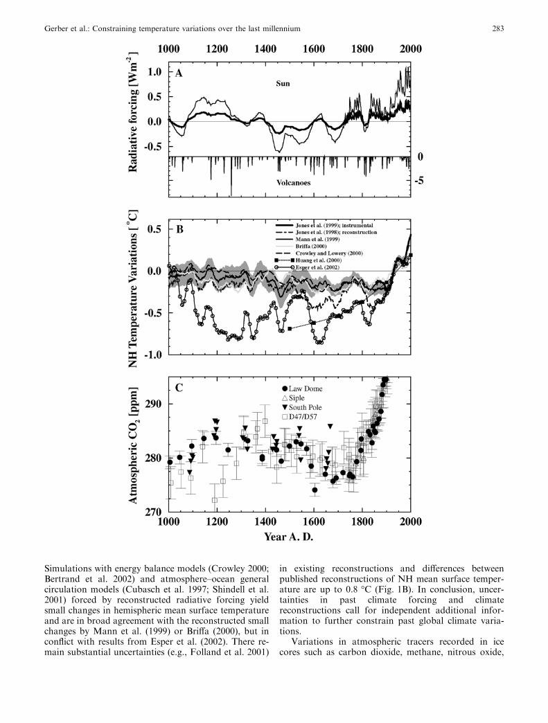
Reconstructions of solar irradiance (Fig. 1A, upperpanel) show a high total solar irradiance (TSI) duringthe 11th and 12th century, and low TSI during 1400 to1700 AD. Distinct minima are found around 1320, 1450,1550, 1680 and 1820 AD. Volcanic forcing (Fig. 1A,lower panel) is negative (cooling) and pulse-like as sulfurinjected into the stratosphere by explosive eruptions isremoved within a few years. Uncertainties in recon-structed radiative forcing, that serves as an input todrive climate models, are large. For example, the role ofsolar variability for climate change has been discussedcontroversially (Ramaswamy et al. 2001). Changes inTSI are reconstructed based on proxy records of solarmagnetic activity such as historically observed sunspotnumbers and the abundance of the cosmogenic radio-isotopes 10Be as recorded in polar ice and 14C as re-corded in tree rings (e.g., Beer et al. 1994; Bard et al.2000). Simple linear scaling has been applied to translatethe radio-isotope records into TSI changes by Bard et al.(2000) and the scaling varies by a factor of 2.6 betweendifferent plausible reconstructions (Fig. 1A). In additionto TSI variations, changes in ultraviolet radiation in-fluence the atmospheric ozone distribution and therebyclimate (Haigh 1996; Thompson and Solomon 2002).Furthermore, it has been speculated that changes insolar magnetic activity itself influence climate (Svens-mark and Friis-Christensen 1997). Similar uncertaintiesexist with regard to past volcanic forcing.

Reconstructions of the Northern Hemisphere (NH)mean surface temperature show distinct cold and warmperiods during the past millennium (Fig. 1B). Most re-constructions suggest that NH mean temperature was

lower than today by a few tenths of a degree (Follandet al. 2001). A recent primarily extratropical recon-struction (Esper et al. 2002) yields more pronouncedtemperature fluctuations and suggests that NH temper-atures have been lower by 0.3 to 1 �C between 1200 ADand 1800 AD as compared to recent decades and a warmperiod around 1000 AD. The timing of cold and warmperiods varies considerably over the globe (Folland et al.2001). Unusually cold and dry winters have been foundin Central Europe during the ‘‘Little Ice Age’’ that wereassociated with lower index states of the Arctic andNorth Atlantic Oscillation patterns during the seven-teenth century (Wanner et al. 1995; Luterbacher et al.1999). On the other hand, recent work by Hendy et al.(2002) suggest little if any cooling at all during the sev-enteenth to nineteenth centuries in the Great BarrierReef sector of the tropical Pacific. Primarily extratropi-cal NH temperature reconstructions exhibit more cool-ing during the seventeenth to nineteenth centuries thanreconstructions based on the full (tropical and extra-tropical) NH (see e.g., Mann et al. 1999; Crowley andLowery 2000; Folland et al. 2001; Esper et al. 2002).Measurements of borehole temperatures (Huang et al.2000) reveal a warming of 0.9 �C since 1500 AD.

Fig. 1A–C Reconstructions of solar and volcanic radiative forcing,NH temperature, and atmospheric CO2 for the last millennium. Atop panel: reconstructed radiative forcing from variations in totalsolar irradiance based on a smoothed cosmonuclides productionrecord (Bard et al. 2000). The different curves have been obtainedwith different scaling factors to match the Maunder Minimum(around 1700) irradiance reduction derived by Reid (1997) (thinsolid line) and by Lean et al. (1995) (thick solid line). This latterreconstruction has been used as standard input in this study. High-frequency variations have been included here for the industrialperiod based on Lean et al. (1995). A Bottom panel, right hand axis:reconstructed radiative forcing from explosive volcanic eruptions(Crowley 2000). Note the different scales between the upper andlower panel. B Reconstructions of Northern Hemisphere (NH)surface temperature variations for the last millennium by Jones etal. (1998) (dot-dashed, summer, extratropical-emphasis), Mann etal. (1999) (thin solid line annual mean, full hemisphere), Briffa(2000) (gray, summer, extra-tropical) Crowley and Lowery (2000)(dashed, summer-emphasis, extratropical), Huang et al. (2000)(squares, borehole temperature, gridded before averaging, takenfrom Briffa and Osborn (2002)) and Esper et al. (2002) (solid line,with circles). The instrumental record (annual mean, full hemi-sphere) is shown by the thick solid line (Jones et al. 1999). All serieshave been smoothed by 31-year running averages. The shaded areaindicates the uncertainty (±2 standard deviation) of the smoothedtemperature reconstruction by Mann et al. (1999). It was computedbased on the use of the standard reduction of variance in theestimate of the mean, �rr ¼

ffiffiffiffiffiffiffiffiffiffiffiffi

r2=N 0p

where r2 is the nominal variancein the annual estimates diagnosed from the calibration residuals,and N¢ is the effective degrees of freedom which is approximately N¢= N/2 in the decadal range, owing to the existence of serialcorrelation in the calibration residuals. C Atmospheric CO2

concentration as measured on air entrapped in ice drilled at LawDome (solid circles) (Etheridge et al. 1996), Siple (open triangles)(Neftel et al. 1985), South Pole (solid triangles) (Siegenthaler et al.1988), and Adelie Land (cores D47 and D57, open squares)(Barnola et al. 1995). The age scale of the South Pole ice core hasbeen shifted by 115 years towards older dates compared to theoriginal publication based on an improved firn-diffusion model(Schwander 1996)

c

282 Gerber et al.: Constraining temperature variations over the last millennium

Simulations with energy balance models (Crowley 2000;Bertrand et al. 2002) and atmosphere–ocean generalcirculation models (Cubasch et al. 1997; Shindell et al.2001) forced by reconstructed radiative forcing yieldsmall changes in hemispheric mean surface temperatureand are in broad agreement with the reconstructed smallchanges by Mann et al. (1999) or Briffa (2000), but inconflict with results from Esper et al. (2002). There re-main substantial uncertainties (e.g., Folland et al. 2001)

in existing reconstructions and differences betweenpublished reconstructions of NH mean surface temper-ature are up to 0.8 �C (Fig. 1B). In conclusion, uncer-tainties in past climate forcing and climatereconstructions call for independent additional infor-mation to further constrain past global climate varia-tions.

Variations in atmospheric tracers recorded in icecores such as carbon dioxide, methane, nitrous oxide,

Gerber et al.: Constraining temperature variations over the last millennium 283

and sulfate provide additional clues on the magnitudeof past climate changes. The ice core records show asmall variability in atmospheric greenhouse gases anddeposited sulfate over the last millennium until theonset of industrialization as compared to measuredvariations over glacial-interglacial cycles, Dansgaard/Oeschger events, or the entire Holocene (Stauffer et al.2002; Bigler et al. 2002). Qualitatively, this suggeststhat averaged over the globe or the NH naturalclimate variations have been modest during the lastmillennium.

CO2 data from several Antarctic ice cores (Fig. 1C)show that atmospheric CO2 varied by less than 15 ppmduring the last millennium until the onset of industrial-ization (Siegenthaler et al. 1988; Barnola et al. 1995;Etheridge et al. 1996). However, the detailed evolution isnot consistent between different cores. For example,results from cores D47/D57 (Barnola et al. 1995) suggestan increase in atmospheric CO2 of around 10 ppmduring 1200 to 1400 AD, whereas the data from LawDome (Etheridge et al. 1996) suggest a small downwardtrend. Similarly, the Law Dome data show a rapid CO2

decrease of about 8 ppm at the end of the sixteenthcentury, which is not found in the other cores. Possiblereasons for these discrepancies are the in-situ transfor-mation of calcite and/or organic carbon to CO2 after theenclosure of air in the ice (Tschumi and Stauffer 2000;Anklin et al. 1995) as well as analytical problems, es-pecially for measurements made in the 1980 and early1990s. In summary, preindustrial atmospheric CO2

variations were small during the last millennium anddetails in the different CO2 ice core records need to beinterpreted with caution.

The outline of this work is as follows. The Bern CCmodel and the experimental setup are described in thenext section. In Sect. 3.1 we present the sensitivity of theterrestrial component of the Bern CC model, the Lund-Potsdam-Jena Dynamic Global Vegetation Model (LPJ-DGVM), to step-like changes in one of the drivingvariables CO2, temperature, precipitation and cloudcover. The adjustment time of atmospheric CO2 to a stepchange in radiative forcing or in climate is explored inSect. 3.2 for the coupled carbon cycle-climate model.The results of the transient simulations for the pastmillennium are presented in Sects. 3.3 and 3.4. In Sect.3.5, we apply the ice core CO2 record to constrain low-frequency variations in NH mean surface temperaturefor the period 1100 to 1700 AD. In Sect. 3.6, we thencompare simulated atmospheric d13C with ice core dataand discuss briefly the relevance of d13C in the climate-carbon cycle system. Discussion and conclusions followin Sect. 4.

2 Model description

The Bern CC model (Joos et al. 2001) consists of a chemistry,radiative forcing, climate, and carbon cycle module. The mainfeatures of the model are summarized.

2.1 Radiative forcing

In simulations over the last millennium (1075 AD to 2000 AD),global-average radiative forcing from solar irradiance changes andexplosive volcanic eruptions are prescribed (Crowley 2000,Fig. 1A) to simulate the evolution of temperature, precipitation,cloud cover, and atmospheric CO2. Radiative forcing by CO2 iscalculated from concentrations assuming a logarithmic relationship(Myhre et al. 1998). Radiative forcing by other anthropogenicgreenhouse gases and aerosols and carbon emissions due to fossilfuel use and land use changes for the industrial period (1700 to2000 AD) are taken into account (Joos et al. 2001).

2.2 Climate model

The model’s climate component is an impulse response-empiricalorthogonal function (IRF-EOF) substitute driven by radiativeforcing. An IRF for surface-to-deep tracer mixing in combinationwith an equation describing air–sea heat exchange and the energybalance at the surface (Joos and Bruno 1996) characterize the ad-justment time of the climate system to changes in radiative forcing,whereas EOFs describe the spatial patterns of the annual meanperturbations in temperature (DT), precipitation (DP), and cloudcover (DCC) (Hooss et al. 2001; Meyer et al. 1999). The climatesensitivity for temperature, defined as the change in global meansurface temperature per radiative forcing unit, is specified here as aterm in the surface energy balance equation (Siegenthaler andOeschger 1984), whereas the climate sensitivity of comprehensivemodels is determined by the strength of the resolved feedbackmechanisms. The spatial patterns (EOFs) in DT, DP, and DCCassociated with global temperature changes resulting from radiativeforcing by greenhouse gases and solar irradiance were derived froma 850-year ‘‘4 · CO2’’ simulation with the ECHAM3/LSG modelwherein atmospheric CO2 was quadrupled in the first 120 years andheld constant thereafter (Voss and Mikolajewicz 2001). The IRFfor surface-to-deep mixing of heat (and other tracers) was derivedfrom the High-Latitude Exchange-Interior Diffusion/Advection(HILDA) model (Joos et al. 1996). The combination of an IRF forsurface-to-deep heat mixing and an energy balance equation allowsus to explicitly simulate the damping effect of ocean heat uptake onmodeled surface temperatures (Hansen et al. 1984), in contrast tothe IRF-EOF model developed by Hooss et al. (2001) that was usedin earlier work with the Bern CC model (Joos et al. 2001). Simu-lations with both IRF approaches yield almost identical results forthe 4 · CO2 experiment when the IRF-EOF models’ climate sen-sitivity for a doubling of atmospheric CO2 is set to 2.5 �C, i.e., thesensitivity of the ECHAM3/LSG. However, when the IRF models’climate sensitivity is increased, temperature changes scale with theclimate sensitivity in the IRF approach by Hooss et al. (2001),whereas in the IRF model used here simulated temperature changesare smaller during the first transient phase of the experiment,because ocean heat uptake is explicitly simulated.

Modeled changes in precipitation and cloud cover are used in apurely diagnostic way and scale linearly with the modeled globalmean surface temperature changes. The climate sensitivities of thesubstitute for a doubling of atmospheric CO2 corresponding to achange in radiative forcing of 3.7 W m–2 are 2.5 �C (global meansurface-air temperature), 64 mm yr–1 (global mean precipitation),and –0.9% (cloud cover) in the standard case. In sensitivity ex-periments, temperature sensitivities of 1.5 �C and 4.5 �C have beenused; the sensitivities of other climate variables were scaled ac-cordingly. We note that for the ECHAM3/LSG pattern deviationsin NH mean are 20% larger than in global mean surface temper-ature and that the temperature deviations averaged over land are36% higher than those averaged over the globe.

The temperature response of each volcanic eruption of the lastmillennium was calculated by multiplying its peak radiative forcing(Crowley 2000) with an observationally based response pattern fortropical and high-latitude volcanoes, respectively. The temperatureanomalies due to volcanic forcing were then linearly combined withthe anomalies calculated by the ECHAM-3/LSG substitute inresponse to solar and CO2 forcing. Changes in precipitation and

284 Gerber et al.: Constraining temperature variations over the last millennium

photosynthetic active radiation in response to explosive volcaniceruptions were neglected. Each peak of the volcanic radiativeforcing series was assigned to either a high latitude or a tropicaleruption using a catalogue of volcanic eruptions (Simkin andSiebert 1994). The average temperature response of tropical andnorthern high-latitude volcanoes was calculated from observations(Jones 1994) following Robock and Mao (1993). First, low-fre-quency variations, and the El Nino/Southern Oscillation signal areremoved from the temperature data and the resulting temperatureanomalies are seasonally averaged. Then, the seasonal temperatureanomalies for the first five years after the eruptions of the tropicalvolcanoes Krakatau (1883), Soufriere (1902)/Santa Maria (1902),El Chichon (1982), and Mt. Pinatubo (1991) were extracted. Theindividual seasonal temperature fields of the four eruptions wereaveraged for each year after the eruptions to obtain a five-year longdata set. Finally, the anomalies were divided by the average of thepeak radiative forcing of the four eruptions. The response ofnorthern high-latitude volcanoes was obtained by repeating thisprocedure for the eruptions of Bandai (1888), Katmai (1912) andBezymianny (1956). Peak radiative forcing of Bandai, which left notrace in the Crowley (2000) series, was calculated using the global-average aerosol optical depth estimate of Sato and Hansen (1992)and the relation of Lacis et al. (1992). We note that conclusionsremain unchanged if the climatic response (temperature, precipi-tation, cloud cover) to explosive volcanic eruptions is calculatedusing the ECHAM3/LSG substitute instead of applying theobservationally based temperature response pattern.

2.3 Carbon cycle model

The carbon cycle component consists of a well-mixed atmosphere,a substitute of the HILDA ocean model (Siegenthaler and Joos1992; Joos et al. 1996), and the LPJ-DGVM (Sitch 2000; Prenticeet al. 2000; Cramer et al. 2001; Joos et al. 2001; McGuire et al.2001; Sitch et al. submitted 2002; Kaplan 2002). Surface-to-deeptracer transport in the ocean substitute is described by an IRF. Thenon-linearities in air–sea gas exchange and carbon chemistry arecaptured by separate equations. The effect of sea-surface warmingon carbonate chemistry is included (Joos et al. 1999b). However,ocean circulation changes are not considered in our standardsimulation.

The LPJ-DGVM is driven by local temperatures, precipitation,incoming solar radiation, cloud cover, and atmospheric CO2. TheLPJ-DGVM simulates the distribution of nine plant functionaltypes (PFTs) based on bioclimatic limits for plant growth and re-generation and plant-specific parameters that govern plant com-petition for light and water. The PFTs considered are tropicalbroad-leaved evergreen trees, tropical broad-leaved raingreen trees,temperate needle-leaved evergreen trees, temperate broad-leavedevergreen trees, temperate broad-leaved summergreen trees, borealneedle-leaved evergreen trees, boreal summergreen trees, C3

grasses/forbs, and C4 grasses. Dispersal processes are not explicitlymodeled and an individual PFT can invade new regions if its bio-climatic limits and competition with other PFTs allow establish-ment. There are seven carbon pools per PFT, representing leaves,sapwood, heartwood, fine-roots, a fast and a slow decomposingabove-ground litter pool, and a below-ground litter pool; and twosoil carbon pools, which receive input from litter of all PFTs.Photosynthesis is as a function of absorbed photosyntheticallyactive radiation, temperature, atmospheric CO2 concentration, daylength, and canopy conductance using a form of the Farquharscheme (Farquhar et al. 1980; Collatz et al. 1992) with leaf-leveloptimized nitrogen allocation (Haxeltine and Prentice 1996) and anempirical convective boundary layer parametrization (Monteith1995) to couple the carbon and water cycles. Soil texture classes areassigned to every grid cell (Zobler 1986), and the soil hydrology issimulated using two soil layers (Haxeltine and Prentice 1996).Decomposition rates of soil and litter organic carbon depend onsoil temperature (Lloyd and Taylor 1994) and moisture (Foley1995). Fire fluxes are calculated based on litter moisture content, afuel load threshold, and PFT specific fire resistances (Thonickeet al. 2001). 13C discrimination during photosynthesis is based

on Lloyd and Farquhar (1994). The spatial resolution of theLPJ-DGVM is set to 3.75� · 2.5�.

2.4 Model spin-up

The LPJ-DGVM is spun up from bare ground under pre-industrialCO2 (281.43 ppm) and a baseline climate that includes inter-annualvariability (Cramer et al. 2001; Leemans and Cramer 1991) for2000 years for idealized sensitivity runs with the LPJ-DGVM aloneand for 4000 years for simulations with the coupled climate-carboncycle model. At year 400, the sizes of the slowly overturning soilcarbon pools are calculated analytically from annual litter inputsand annual mean decomposition rates in order to reduce the nec-essary time to approach the final equilibrium. Then spin-up iscontinued and all pools (including the soil pools) and state vari-ables are continuously updated. The annual average global netecosystem production is less than 1Æ10–2 gigatons of carbon (GtC)after 2000 years and less than 5Æ10–3 GtC after 4000 years of spin-up. In standard simulations the LPJ-DGVM is coupled to the othermodules after spin-up, and the spatial fields in annual mean per-turbations of temperature, cloud cover, and precipitation simulatedby the ECHAM3/LSG substitute and calculated for explosivevolcanic eruptions are added to the baseline climate.

3 Results

3.1 Sensitivity of the dynamic global vegetation modelto changes in temperature, precipitation,and atmospheric CO2

In this section, the sensitivity of the LPJ-DGVM tospatially uniform step-like variations in temperature,precipitation, and atmospheric CO2, is investigated todetermine the importance of individual climate forcingfactors for modeled terrestrial carbon storage. In theidealized sensitivity experiments presented here, the LPJ-DGVM is run alone and atmospheric CO2 and climateare prescribed. A globally or hemispherically uniformperturbation in one of the driving variables (CO2, tem-perature, precipitation) is added to the baseline clima-tology and simulations are continued until a newequilibrium is reached. Results are expressed as devia-tions to a baseline simulation. Experimental setup andresults are summarized in Table 1.

3.1.1 Temperature

The sensitivity of the LPJ-DGVM to variations intemperature is examined with step-like global tempera-ture perturbations by +1 �C and –1 �C, respectively(experiments ST+1 and ST–1). A third experiment ST±1

is a sudden temperature decrease by 1 �C for all gridcells in the NH, and a simultaneous increase by 1 �C inthe Southern Hemisphere (SH) to schematically mimicthe effect of a reduction in the North Atlantic ther-mohaline circulation. We note, however, that paleodataand models suggest that for a reduction in the NorthAtlantic thermohaline circulation SH warming is muchless pronounced than cooling in the Atlantic region. Theatmospheric CO2 is set to a constant value of 281 ppm.

Gerber et al.: Constraining temperature variations over the last millennium 285

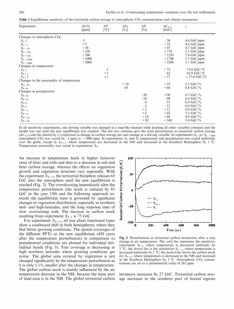
An increase in temperature leads to higher turnoverrates of litter and soils and thus to a decrease in soil andlitter carbon storage, whereas the effects on vegetationgrowth and vegetation structure vary regionally. Withthe experiment ST+1, the terrestrial biosphere releases 65GtC into the atmosphere until the new equilibrium isreached (Fig. 2). The overshooting immediately after thetemperature perturbation (the stock is reduced by 83GtC in the year 150) and the following approach to-wards the equilibrium state is governed by significantchanges in vegetation distribution, especially in northernmid- and high-latitudes, and the long response time ofslow overturning soils. The increase in carbon stockresulting from experiment ST–1 is 75 GtC.

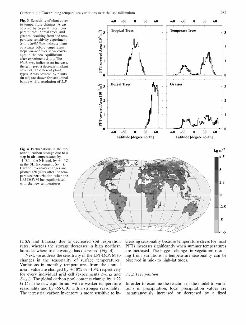
For experiment ST±1, all tree plant functional typesshow a southward shift in both hemispheres, where theyfind better growing conditions. The spatial coverages ofthe different PFTs at the new equilibrium (450 yearsafter the temperature perturbation) in comparison topreindustrial conditions are plotted for individual lati-tudinal bands (Fig. 3). Tree coverage is decreasing athigh northern latitudes where growing conditions getworse. The global area covered by vegetation is notchanged significantly by the temperature perturbation asit is only 1.1% smaller after the changes in temperature.The global carbon stock is mainly influenced by the airtemperature decrease in the NH, because the main partof land area is in the NH. The global terrestrial carbon

inventory increases by 27 GtC. Terrestrial carbon stor-age increases in the southern part of boreal regions

Table 1 Equilibrium sensitivity of the terrestrial carbon storage to atmospheric CO2 concentrations and climate parameters

Experiment DCO2 DT DST DP DCterr c[ppm] [�C] [%] [%] [GtC]

Changes in atmospheric CO2

SC–5 –5 –20 4.0 GtC/ppmSC+5 +5 +23 4.6 GtC/ppmSC+10 +10 +47 4.7 GtC/ppmSC+250 +250 +770 3.1 GtC/ppmSC+500 +500 +1220 2.4 GtC/ppmSC+1000 +1000 +1740 1.7 GtC/ppmSC+2000 +2000 +2280 1.1 GtC/ppmChanges in temperatureST–1 –1 +75 –75.0 GtC/�CST+1 +1 –65 –65.0 GtC/�CST±1 ±1 +27 ±27.0 GtC/�CChanges in the seasonality of temperatureSS+10 +10 +22 2.2 GtC/%SS–10 –10 +66 6.6 GtC/%Changes in precipitationSP–20 –20 –130 6.5 GtC/%SP–14 –14 –90 6.4 GtC/%SP–8 –8 –51 6.4 GtC/%SP–2 –2 –12 6.0 GtC/%SP+2 +2 +12 6.0 GtC/%SP+8 +8 +42 5.3 GtC/%SP+14 +14 +68 4.9 GtC/%SP+20 +20 +100 5.0 GtC/%

In all sensitivity experiments, one driving variable was changed in a step-like manner while keeping all other variables constant and themodel was run until the new equilibrium was reached. The last two columns give the total perturbation in terrestrial carbon storage(DCterr) and the sensitivity (c) expressed as change in carbon storage per unit change in a driving variable. In experiments SC–5to SC+2000

atmospheric CO2 was varied by –5 ppm to +2000 ppm. In experiments ST and SP temperature and precipitation was varied uniformlyover the globe, except in ST±1, where temperature are decreased in the NH and increased in the Southern Hemisphere by 1 �C.Temperature seasonality was varied in experiments SS

Fig. 2 Perturbations in terrestrial carbon inventories after a stepchange in air temperature. The solid line represents the sensitivityexperiment ST–1, where temperature is decreased uniformly by1 �C; the dotted line is the simulation ST+1, where temperature isincreased uniformly by 1 �C; the dashed line shows the carbon stockfor ST±1, where temperature is decreased in the NH and increasedin the Southern Hemisphere by 1 �C. Atmospheric CO2 concen-trations are set to a preindustrial value of 281 ppm

286 Gerber et al.: Constraining temperature variations over the last millennium

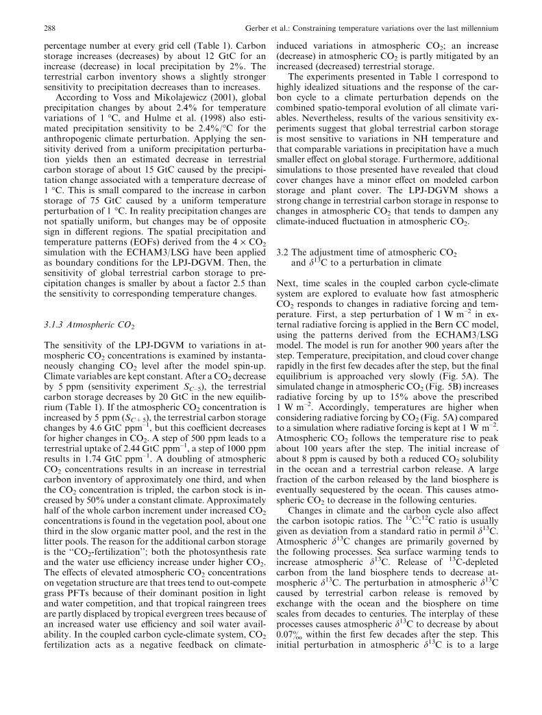
(USA and Eurasia) due to decreased soil respirationrates, whereas the storage decreases in high northernlatitudes where tree coverage has decreased (Fig. 4).

Next, we address the sensitivity of the LPJ-DGVM tochanges in the seasonality of surface temperatures.Variations in monthly temperatures from the annualmean value are changed by +10% or –10% respectivelyfor every individual grid cell (experiments SS+10 andSS–10). The global carbon pool contents change by +22GtC in the new equilibrium with a weaker temperatureseasonality and by –66 GtC with a stronger seasonality.The terrestrial carbon inventory is more sensitive to in-

creasing seasonality because temperature stress for mostPFTs increases significantly when summer temperaturesare increased. The biggest changes in vegetation result-ing from variations in temperature seasonality can beobserved in mid- to high-latitudes.

3.1.2 Precipitation

In order to examine the reaction of the model to varia-tions in precipitation, local precipitation values areinstantaneously increased or decreased by a fixed

Fig. 3 Sensitivity of plant coverto temperature changes. Areascovered by tropical trees, tem-perate trees, boreal trees, andgrasses, resulting from the tem-perature sensitivity experimentST±1. Solid lines indicate plantcoverages before temperaturesteps, dashed lines show cover-ages in the new equilibriumafter experiment ST±1. Theblack area indicates an increase,the gray area a decrease in plantcover of the different planttypes. Areas covered by plants(in m2) are shown for latitudinalbands with a resolution of 2.5�

Fig. 4 Perturbations in the ter-restrial carbon storage due to astep in air temperatures by–1 �C in the NH and, by +1 �Cin the SH (experiment ST±1).Carbon inventory changes areplotted 450 years after the tem-perature perturbation, when theLPJ-DGVM has equilibriatedwith the new temperatures

Gerber et al.: Constraining temperature variations over the last millennium 287

percentage number at every grid cell (Table 1). Carbonstorage increases (decreases) by about 12 GtC for anincrease (decrease) in local precipitation by 2%. Theterrestrial carbon inventory shows a slightly strongersensitivity to precipitation decreases than to increases.

According to Voss and Mikolajewicz (2001), globalprecipitation changes by about 2.4% for temperaturevariations of 1 �C, and Hulme et al. (1998) also esti-mated precipitation sensitivity to be 2.4%/�C for theanthropogenic climate perturbation. Applying the sen-sitivity derived from a uniform precipitation perturba-tion yields then an estimated decrease in terrestrialcarbon storage of about 15 GtC caused by the precipi-tation change associated with a temperature decrease of1 �C. This is small compared to the increase in carbonstorage of 75 GtC caused by a uniform temperatureperturbation of 1 �C. In reality precipitation changes arenot spatially uniform, but changes may be of oppositesign in different regions. The spatial precipitation andtemperature patterns (EOFs) derived from the 4 · CO2

simulation with the ECHAM3/LSG have been appliedas boundary conditions for the LPJ-DGVM. Then, thesensitivity of global terrestrial carbon storage to pre-cipitation changes is smaller by about a factor 2.5 thanthe sensitivity to corresponding temperature changes.

3.1.3 Atmospheric CO2

The sensitivity of the LPJ-DGVM to variations in at-mospheric CO2 concentrations is examined by instanta-neously changing CO2 level after the model spin-up.Climate variables are kept constant. After a CO2 decreaseby 5 ppm (sensitivity experiment SC–5), the terrestrialcarbon storage decreases by 20 GtC in the new equilib-rium (Table 1). If the atmospheric CO2 concentration isincreased by 5 ppm (SC+5), the terrestrial carbon storagechanges by 4.6 GtC ppm–1, but this coefficient decreasesfor higher changes in CO2. A step of 500 ppm leads to aterrestrial uptake of 2.44 GtC ppm–1, a step of 1000 ppmresults in 1.74 GtC ppm–1. A doubling of atmosphericCO2 concentrations results in an increase in terrestrialcarbon inventory of approximately one third, and whenthe CO2 concentration is tripled, the carbon stock is in-creased by 50% under a constant climate. Approximatelyhalf of the whole carbon increment under increased CO2

concentrations is found in the vegetation pool, about onethird in the slow organic matter pool, and the rest in thelitter pools. The reason for the additional carbon storageis the ‘‘CO2-fertilization’’; both the photosynthesis rateand the water use efficiency increase under higher CO2.The effects of elevated atmospheric CO2 concentrationson vegetation structure are that trees tend to out-competegrass PFTs because of their dominant position in lightand water competition, and that tropical raingreen treesare partly displaced by tropical evergreen trees because ofan increased water use efficiency and soil water avail-ability. In the coupled carbon cycle-climate system, CO2

fertilization acts as a negative feedback on climate-

induced variations in atmospheric CO2; an increase(decrease) in atmospheric CO2 is partly mitigated by anincreased (decreased) terrestrial storage.

The experiments presented in Table 1 correspond tohighly idealized situations and the response of the car-bon cycle to a climate perturbation depends on thecombined spatio-temporal evolution of all climate vari-ables. Nevertheless, results of the various sensitivity ex-periments suggest that global terrestrial carbon storageis most sensitive to variations in NH temperature andthat comparable variations in precipitation have a muchsmaller effect on global storage. Furthermore, additionalsimulations to those presented have revealed that cloudcover changes have a minor effect on modeled carbonstorage and plant cover. The LPJ-DGVM shows astrong change in terrestrial carbon storage in response tochanges in atmospheric CO2 that tends to dampen anyclimate-induced fluctuation in atmospheric CO2.

3.2 The adjustment time of atmospheric CO2

and d13C to a perturbation in climate

Next, time scales in the coupled carbon cycle-climatesystem are explored to evaluate how fast atmosphericCO2 responds to changes in radiative forcing and tem-perature. First, a step perturbation of 1 W m–2 in ex-ternal radiative forcing is applied in the Bern CC model,using the patterns derived from the ECHAM3/LSGmodel. The model is run for another 900 years after thestep. Temperature, precipitation, and cloud cover changerapidly in the first few decades after the step, but the finalequilibrium is approached very slowly (Fig. 5A). Thesimulated change in atmospheric CO2 (Fig. 5B) increasesradiative forcing by up to 15% above the prescribed1 W m–2. Accordingly, temperatures are higher whenconsidering radiative forcing by CO2 (Fig. 5A) comparedto a simulation where radiative forcing is kept at 1 W m–2.Atmospheric CO2 follows the temperature rise to peakabout 100 years after the step. The initial increase ofabout 8 ppm is caused by both a reduced CO2 solubilityin the ocean and a terrestrial carbon release. A largefraction of the carbon released by the land biosphere iseventually sequestered by the ocean. This causes atmo-spheric CO2 to decrease in the following centuries.

Changes in climate and the carbon cycle also affectthe carbon isotopic ratios. The 13C:12C ratio is usuallygiven as deviation from a standard ratio in permil d13C.Atmospheric d13C changes are primarily governed bythe following processes. Sea surface warming tends toincrease atmospheric d13C. Release of 13C-depletedcarbon from the land biosphere tends to decrease at-mospheric d13C. The perturbation in atmospheric d13Ccaused by terrestrial carbon release is removed byexchange with the ocean and the biosphere on timescales from decades to centuries. The interplay of theseprocesses causes atmospheric d13C to decrease by about0.07& within the first few decades after the step. Thisinitial perturbation in atmospheric d13C is to a large

288 Gerber et al.: Constraining temperature variations over the last millennium

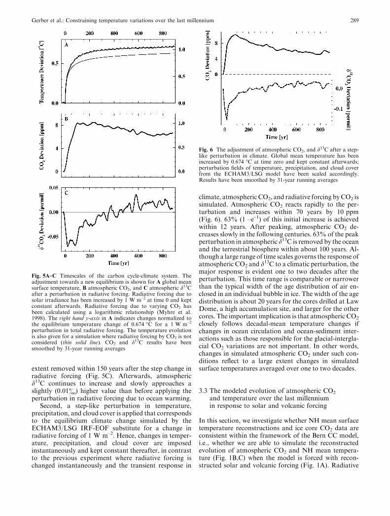
extent removed within 150 years after the step change inradiative forcing (Fig. 5C). Afterwards, atmosphericd13C continues to increase and slowly approaches aslightly (0.01&) higher value than before applying theperturbation in radiative forcing due to ocean warming.

Second, a step-like perturbation in temperature,precipitation, and cloud cover is applied that correspondsto the equilibrium climate change simulated by theECHAM3/LSG IRF-EOF substitute for a change inradiative forcing of 1 W m–2. Hence, changes in temper-ature, precipitation, and cloud cover are imposedinstantaneously and kept constant thereafter, in contrastto the previous experiment where radiative forcing ischanged instantaneously and the transient response in

climate, atmospheric CO2, and radiative forcing byCO2 issimulated. Atmospheric CO2 reacts rapidly to the per-turbation and increases within 70 years by 10 ppm(Fig. 6). 63% (1 –e–1) of this initial increase is achievedwithin 12 years. After peaking, atmospheric CO2 de-creases slowly in the following centuries. 63% of the peakperturbation in atmospheric d13C is removed by the oceanand the terrestrial biosphere within about 100 years. Al-though a large range of time scales governs the response ofatmospheric CO2 and d13C to a climatic perturbation, themajor response is evident one to two decades after theperturbation. This time range is comparable or narrowerthan the typical width of the age distribution of air en-closed in an individual bubble in ice. The width of the agedistribution is about 20 years for the cores drilled at LawDome, a high accumulation site, and larger for the othercores. The important implication is that atmospheric CO2

closely follows decadal-mean temperature changes ifchanges in ocean circulation and ocean-sediment inter-actions such as those responsible for the glacial-intergla-cial CO2 variations are not important. In other words,changes in simulated atmospheric CO2 under such con-ditions reflect to a large extent changes in simulatedsurface temperatures averaged over one to two decades.

3.3 The modeled evolution of atmospheric CO2

and temperature over the last millenniumin response to solar and volcanic forcing

In this section, we investigate whether NH mean surfacetemperature reconstructions and ice core CO2 data areconsistent within the framework of the Bern CC model,i.e., whether we are able to simulate the reconstructedevolution of atmospheric CO2 and NH mean tempera-ture (Fig. 1B,C) when the model is forced with recon-structed solar and volcanic forcing (Fig. 1A). Radiative

Fig. 5A–C Timescales of the carbon cycle-climate system. Theadjustment towards a new equilibrium is shown for A global meansurface temperature, B atmospheric CO2, and C atmospheric d13Cafter a perturbation in radiative forcing. Radiative forcing due tosolar irradiance has been increased by 1 W m–2 at time 0 and keptconstant afterwards. Radiative forcing due to varying CO2 hasbeen calculated using a logarithmic relationship (Myhre et al.1998). The right hand y-axis in A indicates changes normalized tothe equilibrium temperature change of 0.674 �C for a 1 W m–2

perturbation in total radiative forcing. The temperature evolutionis also given for a simulation where radiative forcing by CO2 is notconsidered (thin solid line). CO2 and d13C results have beensmoothed by 31-year running averages

Fig. 6 The adjustment of atmospheric CO2, and d13C after a step-like perturbation in climate. Global mean temperature has beenincreased by 0.674 �C at time zero and kept constant afterwards;perturbation fields of temperature, precipitation, and cloud coverfrom the ECHAM3/LSG model have been scaled accordingly.Results have been smoothed by 31-year running averages

Gerber et al.: Constraining temperature variations over the last millennium 289

forcing from solar irradiance changes and explosivevolcanic eruptions are prescribed in the Bern CC modeland the evolution of temperature, precipitation, cloudcover, atmospheric CO2 and radiative forcing by CO2 issimulated over the past millennium. Radiative forcingby other anthropogenic greenhouse gases and aerosolsand anthropogenic carbon emissions are taken into ac-count for the industrial period.

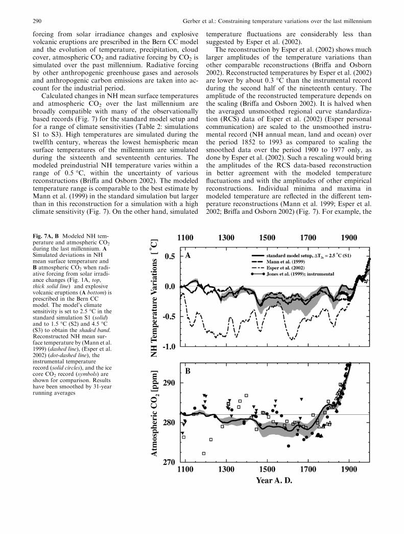
Calculated changes in NH mean surface temperaturesand atmospheric CO2 over the last millennium arebroadly compatible with many of the observationallybased records (Fig. 7) for the standard model setup andfor a range of climate sensitivities (Table 2: simulationsS1 to S3). High temperatures are simulated during thetwelfth century, whereas the lowest hemispheric meansurface temperatures of the millennium are simulatedduring the sixteenth and seventeenth centuries. Themodeled preindustrial NH temperature varies within arange of 0.5 �C, within the uncertainty of variousreconstructions (Briffa and Osborn 2002). The modeledtemperature range is comparable to the best estimate byMann et al. (1999) in the standard simulation but largerthan in this reconstruction for a simulation with a highclimate sensitivity (Fig. 7). On the other hand, simulated

temperature fluctuations are considerably less thansuggested by Esper et al. (2002).

The reconstruction by Esper et al. (2002) shows muchlarger amplitudes of the temperature variations thanother comparable reconstructions (Briffa and Osborn2002). Reconstructed temperatures by Esper et al. (2002)are lower by about 0.3 �C than the instrumental recordduring the second half of the nineteenth century. Theamplitude of the reconstructed temperature depends onthe scaling (Briffa and Osborn 2002). It is halved whenthe averaged unsmoothed regional curve standardiza-tion (RCS) data of Esper et al. (2002) (Esper personalcommunication) are scaled to the unsmoothed instru-mental record (NH annual mean, land and ocean) overthe period 1852 to 1993 as compared to scaling thesmoothed data over the period 1900 to 1977 only, asdone by Esper et al. (2002). Such a rescaling would bringthe amplitudes of the RCS data-based reconstructionin better agreement with the modeled temperaturefluctuations and with the amplitudes of other empiricalreconstructions. Individual minima and maxima inmodeled temperature are reflected in the different tem-perature reconstructions (Mann et al. 1999; Esper et al.2002; Briffa and Osborn 2002) (Fig. 7). For example, the

Fig. 7A, B Modeled NH tem-perature and atmospheric CO2

during the last millennium. ASimulated deviations in NHmean surface temperature andB atmospheric CO2 when radi-ative forcing from solar irradi-ance changes (Fig. 1A, top,thick solid line) and explosivevolcanic eruptions (A bottom) isprescribed in the Bern CCmodel. The model’s climatesensitivity is set to 2.5 �C in thestandard simulation S1 (solid)and to 1.5 �C (S2) and 4.5 �C(S3) to obtain the shaded band.Reconstructed NH mean sur-face temperature by (Mann et al.1999) (dashed line), (Esper et al.2002) (dot-dashed line), theinstrumental temperaturerecord (solid circles), and the icecore CO2 record (symbols) areshown for comparison. Resultshave been smoothed by 31-yearrunning averages

290 Gerber et al.: Constraining temperature variations over the last millennium

minimum around 1475 and the maxima around 1550and 1775 are consistently found in the model results andthe reconstructions by Esper et al. (2002) and Mannet al. (1999). Simulated temperature increases after aminimum in solar and volcanic forcing between 1825and 1865 similar to the reconstruction by Esper et al.(2002) whereas the reconstruction by Mann et al. (1999)shows little change during this period. On the otherhand, minima and maxima of the temperature recon-structions and the model results are to a large degreeout-of-phase during the early part of the millennium.

The modeled global mean surface temperature in-crease over the twentieth century is 0.39 �C, comparableto the estimate of 0.6 ± 0.2 �C derived from instru-mental data (Folland et al. 2001), for the standardsimulation S1 in which the climate sensitivity is set to2.5 �C. The lower than observed surface temperatureincrease modeled for the twentieth century may be dueto an overestimation of the cooling effect by anthropo-genic aerosols (Knutti et al. 2002) in combination with arelatively low climate sensitivity.

Modeled atmospheric CO2 varies within a range of5 ppm before the onset of industrialization in the stan-dard simulation S1, well within the scatter of the ice coredata (Fig. 7B). Simulated CO2 decreases after 1180to reach a first minimum around 1480. Concentrationsremain low during the sixteenth and seventeenth centu-ries. Atmospheric CO2 increases rapidly during the in-dustrial period due to anthropogenic carbon emissions.

In summary, simulated changes in atmospheric CO2

and NH mean surface temperature are broadly

compatible with the ice core CO2 data and with tem-perature reconstructions.

3.4 Sensitivity of NH temperature and atmosphericCO2 to forcings and carbon cycle processes

The importance of individual mechanisms and forcingsfor the modeled changes in climate and CO2 is investi-gated (simulations S4 to S9, Fig. 8) and the contributionof natural climate forcing to the rise in atmospheric CO2

over the industrial period is investigated (simulationsS10 and S11, Fig. 9).

Volcanic forcing contributes substantially to the lowtemperatures and low CO2 values during the sixteenthand seventeenth centuries. Atmospheric CO2 decreasesby 2.8 ppm between 1180 and 1480 AD in simulation S4,where volcanic forcing is excluded, compared to4.1 ppm in S1. In S4, simulated NH mean surface tem-perature and atmospheric CO2 start to increase alreadyaround 1550.

The CO2 decrease during the first half of the millen-nium results from both an increase in global terrestrialcarbon storage and an increase in the CO2 solubility inocean surface waters in response to cooling. Atmo-spheric CO2 decreases by 2.3 ppm between 1180 AD and1480 AD in simulation S5 where terrestrial carbonstorage is kept constant. In simulation S6 where theocean surface temperature is kept constant, the reduc-tion in atmospheric CO2 is 3.1 ppm between 1180 and1480 AD.

Table 2 Simulated temperature and CO2 variations for different model setups

Simulation DT2x NHDT(1180–1480) DCO2 (1180–1480)

Standard model setup (Fig. 7)Standard model configuration with coupled radiative forcing, climate, and carbon cycle modules; reconstructed solar and volcanicradiative forcing prescribed (Fig. 1A); variations in climate and atmospheric CO2 calculated.(S1) Standard climate sensitivity 2.5 �C 0.42 �C 4.1 ppm(S2) Low climate sensitivity 1.5 �C 0.30 �C 2.5 ppm(S3) High climate sensitivity 4.5 �C 0.58 �C 6.8 ppm

Sensitivity experiments (Fig. 8)(S4) Radiative forcing by volcanoes omitted 2.5 �C 0.21 �C 2.8 ppm(S5) Terrestrial carbon storage kept constant 2.5 �C 0.41 �C 2.3 ppm(S6) Sea surface temperature kept constant 2.5 �C 0.41 �C 3.1 ppm

Suppressed terrestrial CO2 fertilization(S7) Standard climate sensitivity 2.5 �C 0.44 �C 8.2 ppm(S8) Low climate sensitivity 1.5 �C 0.36 �C 4.9 ppm(S9) High climate sensitivity 4.5 �C 0.63 �C 11.0 ppm

Anthropogenic impact (Fig. 9)(S10) Anthropogenic emissions omitted 2.5 �C 0.42 �C 4.1 ppm(S11) Pre-industrial land use emissions scaled to population growth 2.5 �C 0.41 �C 3.2 ppm

Variations in radiative forcing (Fig. 11)Solar radiative forcing is multiplied by a factor of 2.6 (Fig. 1A, thin line)(S12) Standard climate sensitivity 2.5 �C 0.74 �C 8.0 ppm(S13) Low climate sensitivity 1.5 �C 0.53 �C 5.8 ppm(S14) High climate sensitivity 4.5 �C 1.00 �C 10.9 ppm(S15) Solar radiative forcing multiplied by a factor of 5 4.5 �C 1.65 �C 18.8 ppm

The climate sensitivity (DT2x) applied in the simulations (S1) to (S15) is shown in the first data column. Simulated differences in NH meansurface temperature (NH DT) and atmospheric CO2 (DCO2) have been evaluated for the relative maximum around 1180 AD and therelative minimum around 1480 AD

Gerber et al.: Constraining temperature variations over the last millennium 291

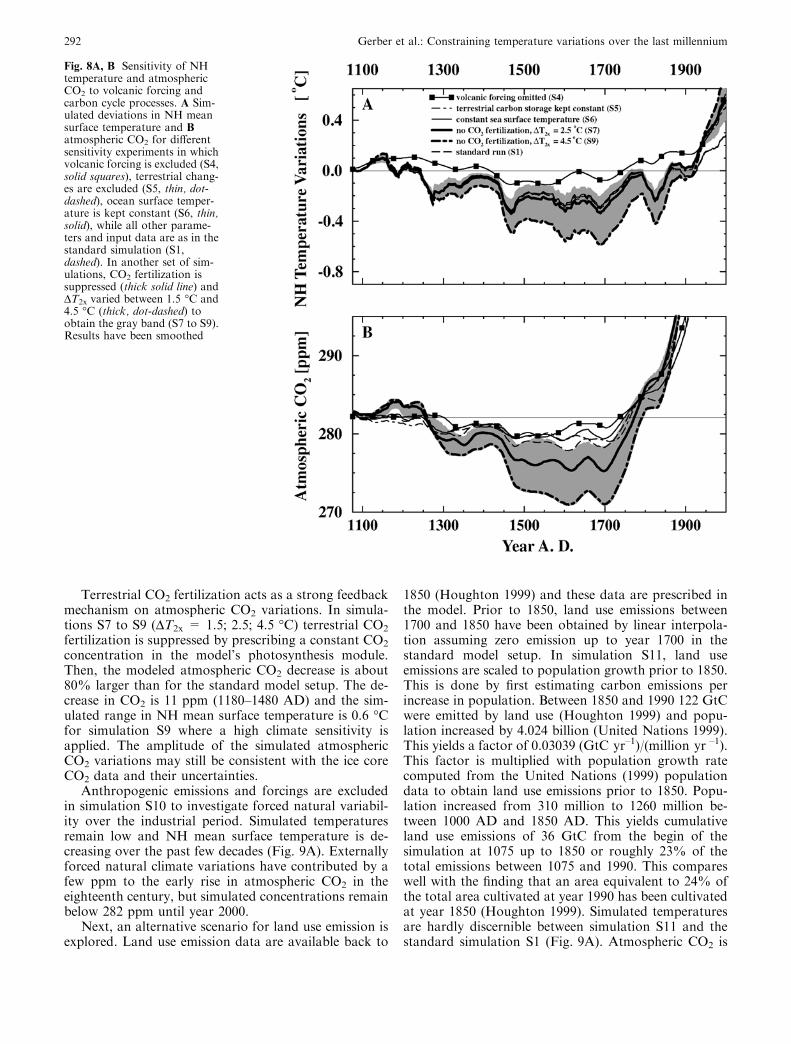
Terrestrial CO2 fertilization acts as a strong feedbackmechanism on atmospheric CO2 variations. In simula-tions S7 to S9 (DT2x = 1.5; 2.5; 4.5 �C) terrestrial CO2

fertilization is suppressed by prescribing a constant CO2

concentration in the model’s photosynthesis module.Then, the modeled atmospheric CO2 decrease is about80% larger than for the standard model setup. The de-crease in CO2 is 11 ppm (1180–1480 AD) and the sim-ulated range in NH mean surface temperature is 0.6 �Cfor simulation S9 where a high climate sensitivity isapplied. The amplitude of the simulated atmosphericCO2 variations may still be consistent with the ice coreCO2 data and their uncertainties.

Anthropogenic emissions and forcings are excludedin simulation S10 to investigate forced natural variabil-ity over the industrial period. Simulated temperaturesremain low and NH mean surface temperature is de-creasing over the past few decades (Fig. 9A). Externallyforced natural climate variations have contributed by afew ppm to the early rise in atmospheric CO2 in theeighteenth century, but simulated concentrations remainbelow 282 ppm until year 2000.

Next, an alternative scenario for land use emission isexplored. Land use emission data are available back to

1850 (Houghton 1999) and these data are prescribed inthe model. Prior to 1850, land use emissions between1700 and 1850 have been obtained by linear interpola-tion assuming zero emission up to year 1700 in thestandard model setup. In simulation S11, land useemissions are scaled to population growth prior to 1850.This is done by first estimating carbon emissions perincrease in population. Between 1850 and 1990 122 GtCwere emitted by land use (Houghton 1999) and popu-lation increased by 4.024 billion (United Nations 1999).This yields a factor of 0.03039 (GtC yr–1)/(million yr –1).This factor is multiplied with population growth ratecomputed from the United Nations (1999) populationdata to obtain land use emissions prior to 1850. Popu-lation increased from 310 million to 1260 million be-tween 1000 AD and 1850 AD. This yields cumulativeland use emissions of 36 GtC from the begin of thesimulation at 1075 up to 1850 or roughly 23% of thetotal emissions between 1075 and 1990. This compareswell with the finding that an area equivalent to 24% ofthe total area cultivated at year 1990 has been cultivatedat year 1850 (Houghton 1999). Simulated temperaturesare hardly discernible between simulation S11 and thestandard simulation S1 (Fig. 9A). Atmospheric CO2 is

Fig. 8A, B Sensitivity of NHtemperature and atmosphericCO2 to volcanic forcing andcarbon cycle processes. A Sim-ulated deviations in NH meansurface temperature and Batmospheric CO2 for differentsensitivity experiments in whichvolcanic forcing is excluded (S4,solid squares), terrestrial chang-es are excluded (S5, thin, dot-dashed), ocean surface temper-ature is kept constant (S6, thin,solid), while all other parame-ters and input data are as in thestandard simulation (S1,dashed). In another set of sim-ulations, CO2 fertilization issuppressed (thick solid line) andDT2x varied between 1.5 �C and4.5 �C (thick, dot-dashed) toobtain the gray band (S7 to S9).Results have been smoothed

292 Gerber et al.: Constraining temperature variations over the last millennium

only slightly higher in simulation S11 than in the stan-dard simulation prior to 1800 (Fig. 9B). This suggeststhat assumptions about land use emissions are not crit-ical for this study.

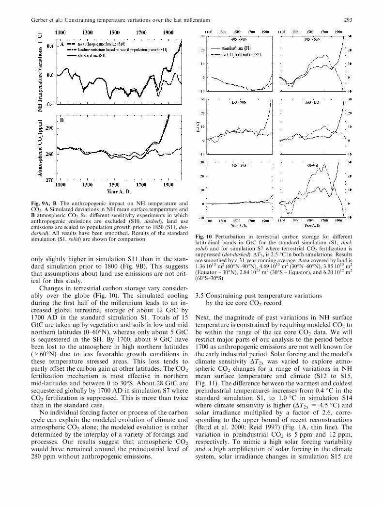
Changes in terrestrial carbon storage vary consider-ably over the globe (Fig. 10). The simulated coolingduring the first half of the millennium leads to an in-creased global terrestrial storage of about 12 GtC by1700 AD in the standard simulation S1. Totals of 15GtC are taken up by vegetation and soils in low and midnorthern latitudes (0–60�N), whereas only about 5 GtCis sequestered in the SH. By 1700, about 9 GtC havebeen lost to the atmosphere in high northern latitudes(>60�N) due to less favorable growth conditions inthese temperature stressed areas. This loss tends topartly offset the carbon gain at other latitudes. The CO2

fertilization mechanism is most effective in northernmid-latitudes and between 0 to 30�S. About 28 GtC aresequestered globally by 1700 AD in simulation S7 whereCO2 fertilization is suppressed. This is more than twicethan in the standard case.

No individual forcing factor or process of the carboncycle can explain the modeled evolution of climate andatmospheric CO2 alone; the modeled evolution is ratherdetermined by the interplay of a variety of forcings andprocesses. Our results suggest that atmospheric CO2

would have remained around the preindustrial level of280 ppm without anthropogenic emissions.

3.5 Constraining past temperature variationsby the ice core CO2 record

Next, the magnitude of past variations in NH surfacetemperature is constrained by requiring modeled CO2 tobe within the range of the ice core CO2 data. We willrestrict major parts of our analysis to the period before1700 as anthropogenic emissions are not well known forthe early industrial period. Solar forcing and the model’sclimate sensitivity DT2x was varied to explore atmo-spheric CO2 changes for a range of variations in NHmean surface temperature and climate (S12 to S15,Fig. 11). The difference between the warmest and coldestpreindustrial temperatures increases from 0.4 �C in thestandard simulation S1, to 1.0 �C in simulation S14where climate sensitivity is higher (DT2x = 4.5 �C) andsolar irradiance multiplied by a factor of 2.6, corre-sponding to the upper bound of recent reconstructions(Bard et al. 2000; Reid 1997) (Fig. 1A, thin line). Thevariation in preindustrial CO2 is 5 ppm and 12 ppm,respectively. To mimic a high solar forcing variabilityand a high amplification of solar forcing in the climatesystem, solar irradiance changes in simulation S15 are

Fig. 10 Perturbation in terrestrial carbon storage for differentlatitudinal bands in GtC for the standard simulation (S1, thicksolid) and for simulation S7 where terrestrial CO2 fertilization issuppressed (dot-dashed). DT2x is 2.5 �C in both simulations. Resultsare smoothed by a 31-year running average. Area covered by land is1.36Æ1013 m2 (60�N–90�N), 4.69Æ1013 m2 (30�N–60�N), 3.85Æ1013 m2

(Equator – 30�N), 2.84Æ1013 m2 (30�S – Equator), and 6.20Æ1012 m2

(60�S–30�S)

Fig. 9A, B The anthropogenic impact on NH temperature andCO2. A Simulated deviations in NH mean surface temperature andB atmospheric CO2 for different sensitivity experiments in whichanthropogenic emissions are excluded (S10, dashed), land useemissions are scaled to population growth prior to 1850 (S11, dot-dashed). All results have been smoothed. Results of the standardsimulation (S1, solid) are shown for comparison

Gerber et al.: Constraining temperature variations over the last millennium 293

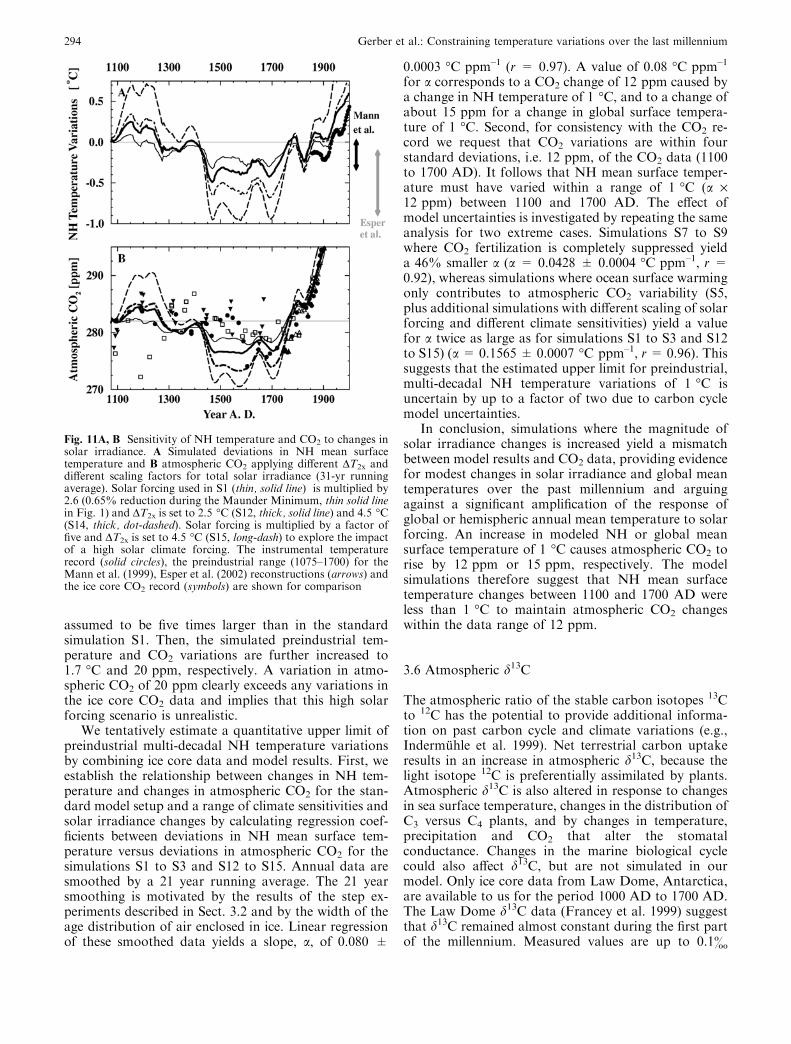
assumed to be five times larger than in the standardsimulation S1. Then, the simulated preindustrial tem-perature and CO2 variations are further increased to1.7 �C and 20 ppm, respectively. A variation in atmo-spheric CO2 of 20 ppm clearly exceeds any variations inthe ice core CO2 data and implies that this high solarforcing scenario is unrealistic.

We tentatively estimate a quantitative upper limit ofpreindustrial multi-decadal NH temperature variationsby combining ice core data and model results. First, weestablish the relationship between changes in NH tem-perature and changes in atmospheric CO2 for the stan-dard model setup and a range of climate sensitivities andsolar irradiance changes by calculating regression coef-ficients between deviations in NH mean surface tem-perature versus deviations in atmospheric CO2 for thesimulations S1 to S3 and S12 to S15. Annual data aresmoothed by a 21 year running average. The 21 yearsmoothing is motivated by the results of the step ex-periments described in Sect. 3.2 and by the width of theage distribution of air enclosed in ice. Linear regressionof these smoothed data yields a slope, a, of 0.080 ±

0.0003 �C ppm–1 (r = 0.97). A value of 0.08 �C ppm–1

for a corresponds to a CO2 change of 12 ppm caused bya change in NH temperature of 1 �C, and to a change ofabout 15 ppm for a change in global surface tempera-ture of 1 �C. Second, for consistency with the CO2 re-cord we request that CO2 variations are within fourstandard deviations, i.e. 12 ppm, of the CO2 data (1100to 1700 AD). It follows that NH mean surface temper-ature must have varied within a range of 1 �C (a ·12 ppm) between 1100 and 1700 AD. The effect ofmodel uncertainties is investigated by repeating the sameanalysis for two extreme cases. Simulations S7 to S9where CO2 fertilization is completely suppressed yielda 46% smaller a (a = 0.0428 ± 0.0004 �C ppm–1, r =0.92), whereas simulations where ocean surface warmingonly contributes to atmospheric CO2 variability (S5,plus additional simulations with different scaling of solarforcing and different climate sensitivities) yield a valuefor a twice as large as for simulations S1 to S3 and S12to S15) (a = 0.1565 ± 0.0007 �C ppm–1, r = 0.96). Thissuggests that the estimated upper limit for preindustrial,multi-decadal NH temperature variations of 1 �C isuncertain by up to a factor of two due to carbon cyclemodel uncertainties.

In conclusion, simulations where the magnitude ofsolar irradiance changes is increased yield a mismatchbetween model results and CO2 data, providing evidencefor modest changes in solar irradiance and global meantemperatures over the past millennium and arguingagainst a significant amplification of the response ofglobal or hemispheric annual mean temperature to solarforcing. An increase in modeled NH or global meansurface temperature of 1 �C causes atmospheric CO2 torise by 12 ppm or 15 ppm, respectively. The modelsimulations therefore suggest that NH mean surfacetemperature changes between 1100 and 1700 AD wereless than 1 �C to maintain atmospheric CO2 changeswithin the data range of 12 ppm.

3.6 Atmospheric d13C

The atmospheric ratio of the stable carbon isotopes 13Cto 12C has the potential to provide additional informa-tion on past carbon cycle and climate variations (e.g.,Indermuhle et al. 1999). Net terrestrial carbon uptakeresults in an increase in atmospheric d13C, because thelight isotope 12C is preferentially assimilated by plants.Atmospheric d13C is also altered in response to changesin sea surface temperature, changes in the distribution ofC3 versus C4 plants, and by changes in temperature,precipitation and CO2 that alter the stomatalconductance. Changes in the marine biological cyclecould also affect d13C, but are not simulated in ourmodel. Only ice core data from Law Dome, Antarctica,are available to us for the period 1000 AD to 1700 AD.The Law Dome d13C data (Francey et al. 1999) suggestthat d13C remained almost constant during the first partof the millennium. Measured values are up to 0.1&

Fig. 11A, B Sensitivity of NH temperature and CO2 to changes insolar irradiance. A Simulated deviations in NH mean surfacetemperature and B atmospheric CO2 applying different DT2x anddifferent scaling factors for total solar irradiance (31-yr runningaverage). Solar forcing used in S1 (thin, solid line) is multiplied by2.6 (0.65% reduction during the Maunder Minimum, thin solid linein Fig. 1) and DT2x is set to 2.5 �C (S12, thick, solid line) and 4.5 �C(S14, thick, dot-dashed). Solar forcing is multiplied by a factor offive and DT2x is set to 4.5 �C (S15, long-dash) to explore the impactof a high solar climate forcing. The instrumental temperaturerecord (solid circles), the preindustrial range (1075–1700) for theMann et al. (1999), Esper et al. (2002) reconstructions (arrows) andthe ice core CO2 record (symbols) are shown for comparison

294 Gerber et al.: Constraining temperature variations over the last millennium

higher during the eighteenth than during the sixteenthcentury (Fig. 12). This has been interpreted as an indi-cation of an increased terrestrial storage in response tocool temperatures (Trudinger et al. 1999; Joos et al.1999a). However, the discrepancies between the LawDome data and other recent state-of-the-art measure-ments on ice from Dome Fuji, Antarctica, (Kawamuraet al. 2000) suggest that small d13C variations must beinterpreted with caution.

Simulated preindustrial atmospheric d13C variations(31-year average) are smaller than 0.05& in the standardsimulation (S1) and less than 0.25& in simulation S15,with a high climate sensitivity and extreme solar forcing(Fig. 12). Simulated and reconstructed d13C decreaserapidly during the industrial period due to the input of13C depleted CO2 from fossil fuel burning and land useemissions. We conclude that available d13C ice core datado currently not allow us to further constrain pastvariations in NH temperature.

4 Conclusion and discussion

In this study, we have evaluated the response of the BernCC model by comparing simulated with reconstructedvariations in NH mean surface temperature and atmo-spheric CO2 over the last millennium. We find reasonablecompatibility between simulated and reconstructed vari-ations in temperature and atmospheric CO2 given theuncertainties in the reconstructions and in reconstructedradiative forcing that is used as input in our model.

An implicit assumption in our modeling approach isthat past, externally forced, low-frequency variations in

temperature and precipitation have the same regionalpatterns as obtained for anthropogenic greenhouse gasforcing. Regional changes in temperature and precipi-tation have been calculated by scaling the computedevolution of global mean temperature changes withtime-invariant patterns derived from a GHG-only ex-periment with the ECHAM3/LSG. Spatial dissimilari-ties between the climatic responses to increased solarforcing and increased CO2 are found regionally inAOGCM simulations (Marshall et al. 1994). However,Cubasch et al. (2001) report that the spatial patternsfound in global warming simulations with and withoutdirect sulfate aerosol forcing obtained with the sameAOGCM are more similar to each other than to thepatterns obtained by other AOGCMs. This indicatesthat the individual response characteristics of the vari-ous AOGCMs are dominating the response patternrather than differences in the forcing. Marshall et al.(1994) and Cubasch et al. (1997) found in AOGCMsimulations forced by reconstructed irradiance changestemperature variations in both hemispheres to be inphase and a temperature pattern similar to that obtainedin simulations with changing CO2 only. Cubasch et al.(1997) and Shindell et al. (2001) both report an enhancedtemperature contrast between land and ocean withwarming over the continents and large parts of the globeand cooling over some parts of the North Atlantic andNorth Pacific under increased solar irradiance, roughlyconsistent with the pattern associated with CO2 forcing.Different climate models yield different regional changesin temperature and precipitation, which could implyimportant differences in the response of the terrestrialbiosphere to global climate change. Leemans et al.(2002) found differences of less than 2% in simulatedatmospheric CO2 when applying temperature and pre-cipitation patterns from four different AOGCMs inemission scenarios.

Changes in the thermohaline circulation are notconsidered in our model. Bond et al. (2001) suggestbased on proxy data that reduced solar irradiance leadsto a reduced formation rate of North Atlantic DeepWater (NADW) and less heat transport into the NorthAtlantic region. The modeling study of Delworth andDixon (2000) demonstrates that moderate changes in thethermohaline circulation, as inferred by Bond et al.(2001), could be driven by changes in the state of theArctic Oscillation. The negative Arctic Oscillationanomaly found by Shindell et al. (2001) during coldphases in their model is then consistent with a moderatereduction in the NADW formation rate suggested byBond et al. (2001). A moderate reduction in NADWformation implies additional moderate cooling in theNorth Atlantic region and a hardly detectable warmingin the SH (Stocker 1998; Marchal et al. 1999a). Moreclearly, Broecker (2001) argues that the ‘‘MedievalWarm Period’’ and the ‘‘Little Ice Age’’ primarily reflectchanges in the thermohaline circulation and that tem-peratures varied in opposite direction in the NH and SH.However, evidence from ocean sediment cores for a

Fig. 12 Measured versus modeled atmospheric d13C. Measuredd13C (permil) values are from air entrapped in ice drilled at LawDome (Francey et al. 1999), Siple Station (Friedli et al. 1986), Dye3 (Leuenberger 1992) and Dome Fuji (Kawamura et al. 2000) andmodel results from the standard simulation S1 (solid) andsimulation S15 where solar forcing is multiplied by a factor offive and DT2x set to 4.5 �C (dashed). Results have been smoothed

Gerber et al.: Constraining temperature variations over the last millennium 295

significant variability in the ocean thermohaline circu-lation during the past millennium as well as evidence foran anti-phase relationship between temperature varia-tions in the NH and SH remain ambiguous or evencontradictory (Keigwin and Boyle 2000; Bradley et al.2001; Hendy et al. 2002). Earlier ocean model results(Joos et al. 1999b; Marchal et al. 1999b; Plattner et al.2001) suggest, in agreement with ice core CO2 results(Stauffer et al. 1998; Marchal et al. 1999b), that evenstrong changes in NADW formation have a small in-fluence on atmospheric CO2 on decadal-to-centennialtime scales. Furthermore, simulations with a zonallyaveraged dynamical ocean model coupled to energy- andmoisture-balance model of the atmosphere yield littlechanges in atmospheric CO2 and NADW over the lastmillennium when driven with reconstructed forcing(Plattner et al. 2002).

The ice core record of atmospheric CO2 has been usedto constrain the magnitude of natural low-frequencytemperature variability during the last millennium. Ourresults are in agreement with reconstructions that suggestmodest variations in NH mean temperature. Our resultsare neither compatible with large changes in solar irradi-ance nor with a strong amplification of solar forcing byfeedbacks within the climate system such as enhancedcloud formation (Svensmark andFriis-Christensen 1997).This supports earlier findings that solar variability hascontributed relatively little to the observed twentiethcentury warming and that most of the twentieth centurywarming is due to anthropogenic forcing (Mitchell et al.2001).

A quantitative upper bound for natural low-fre-quency temperature variations during the last millenni-um has been estimated by requiring that simulatedatmospheric CO2 changes are not larger than four timesthe standard deviation of the ice core data. This is aconservative criterion as a significant part of the scatterin the CO2 data shown in Fig. 1C probably reflects an-alytical problems. For example, recent measurements onremaining ice from the South Pole core show a largelyreduced variability (Siegenthaler 2002). This suggeststhat the current ice core record can be improved sig-nificantly. We propose that a new core be analyzed froma site with low temperatures, a relatively high accumu-lation, low deposition rates of carbonates and otherimpurities, and low levels of oxidants such as H2O2

(Tschumi and Stauffer 2000) to obtain a high resolutionCO2 record over the last millennium.

The quantification of past temperature variationsusing the ice core record depends critically on the ap-plied model. Here, we have used a simplified carboncycle – climate model. This has allowed us to performmany simulations and to explore systematically thesensitivities and time scales of the coupled climate-car-bon cycle model. It also yields clearly defined climaticperturbations to drive the carbon cycle model compo-nent. However, the model includes simplifications andimportant processes may not, or not adequately, bedescribed. For example, internal, unforced climate

variability has not been considered. Similarly, simulatedterrestrial carbon uptake (release) differs between dif-ferent DGVMs for a particular climate forcing. Keysimulations of this study should be repeated using othercarbon cycle-climate models including comprehensivemodels (Cox et al. 2000; Friedlingstein et al. 2000).

Acknowledgements This work was supported by the Swiss Na-tional Science Foundation and the Electric Power Research Insti-tute, Palo Alto, Ca. We thank Thomas Crowley for providingradiative forcing data, Jan Esper for providing his RCS tree ringdata, Kasper Plattner for making available results of his millenni-um simulation, Jakob Schwander for a revised age-scale of theSouth Pole ice core, Urs Siegenthaler for sharing his preliminaryCO2 measurements, and the Lund-Potsdam-Jena Model group formany stimulating discussions and for making the LPJ-DGVMavailable.

References

Anklin M, Barnola JM, Schwander J, Stauffer B, Raynaud D(1995) Processes affecting the CO2 concentration measured inGreenland ice. Tellus Ser B 47: 461–470

Bard E, Raisbeck G, Yiou F, Jouzel J (2000) Solar irradianceduring the last 1200 years based on cosmogenic nuclides. Tellus52 Ser B: 985–992

Barnola JM, Anklin M, Procheron J, Raynaud D, Schwander J,Stauffer B (1995) CO2 evolution during the last millennium asrecorded by Antarctic and Greenland ice. Tellus Ser B 47: 264–272

Beer J, Joos F, Lukasczyk C, Mende W, Rodriguez J, SiegenthalerU, Stellmacher R (1994) 10Be as an indicator of solar variabilityand climate. In: Nesme-Ribes E (ed) The solar engine and itsinfluence on terrestrial atmosphere and climate, Springer, Hei-delberg, Berlin New York, pp 221–223

Bertrand C, Loutre MF, Crucifix M (2002) Climate of the lastmillennium: a sensitivity study. Tellus 54 Ser A: 221–224

Bigler MD, Wagenbach D, Fischer H, Kipfstuhl S, Miller H,Sommer S, Stauffer B (2002) Sulphate record from a northeastGreenland ice core over the last 1200 years based on continuousflow analysis. Ann Glaciol (in press)

Bond G, Kromer B, Beer J, Muscheler R, Evans MN, Showers W,Hoffmann S, Lotti-Bond R, Hajdas I, Bonani G (2001) Per-sistent solar influence on North Atlantic climate during theHolocene. Science 294: 2130–2136

Bradley RS, Briffa KR, Crowley TJ, Hughes MK, Jones PD, MannME (2001) The scope ofMedieval warming. Science 292: 211–212

Briffa KR (2000) Annual climate variability in the Holocene: in-terpreting the message of ancient trees. Quat Sci Rev 19: 87–105

Briffa KR, Jones PD, Schweingruber FH, Osborn TJ (1998) In-fluence of volcanic eruptions on Northern Hemisphere summertemperature over the past 600 years. Nature 393: 450–455

Briffa KR, Osborn TJ (2002) Blowing hot and cold. Science 295:22–27

Broecker WS (2001) Was the Medieval Warm Period global?Science 291: 1497–1499

Collatz GJ, Ribas-Carbo M, Berry JA (1992) A coupled photo-synthesis – stomatal conductance model for leaves of C4 plants.Aust J Plant Physiol 19: 519–538

Cox P, Betts R, Jones C, Spall S, Totterdell I (2000) Acceleration ofglobal warming due to carbon cycle feedbacks in a coupledclimate model. Nature 408: 184–187

Cramer W, Bondeau A, Woodward FI, Prentice IC, Betts RA,Brovkin V, Cox PM, Fisher V, Foley JA, Friend AD, Kucharik C,Lomas MR, Ramankutty N, Sitch S, Smith B, White A,Young-Molling C (2001) Global response of terrestrial ecosys-tem structure and function to CO2 and climate change: resultsfrom six dynamic global vegetation models. Global Change Biol7: 357–373

296 Gerber et al.: Constraining temperature variations over the last millennium

Crowley TJ (2000) Causes of climate change of the last 1000 years.Science 289: 270–277

Crowley TJ, Lowery T (2000) How warm was the Medieval warmperiod? Ambio 29: 51–54

Cubasch U, Meehl GA, Boer GJ, Stouffer RJ, Dix M, Noda A,Senior CA, Raper S, Yap KS (2001) Projections of future cli-mate change. In: Houghton JT, Ding Y, Griggs D, Noguer M,van der Linden P, Dai X, Maskell K, Johnson CA (eds) Climatechange 2001: The scientific basis. Contribution of WorkingGroup I to the Third Assessment Report of the Intergovern-mental Panel on Climate change, Cambridge University Press,Cambridge, United Kingdom pp 525–582

Cubasch UR, Voss R, Hegerl GC, Waszkewitz J, Crowley TJ(1997) Simulation of the influence of solar radiation variationson the global climate with an ocean–atmosphere general cir-culation model. Clim Dyn 13: 757–767

Delworth TL, Dixon KW (2000) Implications of the recent trend inthe Arctic/North Atlantic Oscillation for the North Atlanticthermohaline circulation. J Clim 13: 3721–3727

Esper J, Cook ER, Schweingruber FH (2002) Low-frequency sig-nals in long tree-ring chronologies for reconstructing pasttemperature variability. Science 295: 2250–2253

Etheridge DM, Steele LP, Langenfelds RL, Francey RJ, BarnolaJM, Morgan VI (1996) Natural and anthropogenic changes inatmospheric CO2 over the last 1000 years from air in Antarcticice and firn. J Geophys Res 101: 4115–4128

Farquhar GD, von Caemmerer S, Berry JA (1980) A biochemicalmodel of photosynthetic CO2 assimilation in leaves of C3 spe-cies. Planta 149: 78–90

Foley J (1995) An equilibrium model of the terrestrial carbonbudget. Tellus 47B: 310–319

Folland CK, Karl TR, Christy JR, Clarke RA, Gruza GV, Jouzel J,Mann ME, Oerlemans J, Salinger MJ, Wang SW (2001) Ob-served climate variability and change. In: Houghton JT, DingY, Griggs D, Noguer M, van der Linden P, Dai X, Maskell K,Johnson CA (eds) Climate Change 2001: The Scientific Basis.Contribution of Working Group I to the Third AssessmentReport of the Intergovernmental Panel on Climate Change,Cambridge University Press, Cambridge, United Kingdom, pp99–181

Francey RJ, Allison CE, Etheridge DM, Trudinger CM, EntingIG, Leuenberger M, Langenfelds RL, Michel E, Steele LP(1999) A 1000 year high precision record of d13C in atmosphericCO2. Tellus Ser B 51: 170–193

Friedli H, Loetscher H, Oeschger H, Siegenthaler U, Stauffer B(1986) Ice core record of the 13C/12C ratio of atmosphericcarbon dioxide in the past two centuries. Nature 324: 237–238

Friedlingstein P, Bopp L, Ciais P, Fairhead JLDL, LeTreut H,Monfray P, Orr J (2000) Positive feedback of the carbon cycleon future climate change. Tech Rep 19, Note du Pole deModelisation, Institute Pierre Simon Laplace, France

Haigh JD (1996) The impact of solar variability on climate. Science272: 981–984

Hansen J, Lacis A, Rind D, Russell G, Stone P, Fung I, Ruedy R,Lerner J (1984) Climate sensitivity: analysis of feedbackmechanisms. Climate Processes and Climate Sensitivity,vol Geophysical Monograph 29, American Geophysical Union,pp 130–163

Haxeltine A, Prentice IC (1996) BIOME 3: an equilibrium terres-trial biosphere model based on ecophysiological constraints,resource availability and competition among plant functionaltypes. Global Biogeochem Cycles 10: 693–703

Hendy EJ, Gagan MK, Alibert CA, McCulloch MT, Lough JM,Isdale PJ (2002) Abrupt decrease in tropical Pacific sea surfacesalinity at end of Little Ice Age. Science 295: 1511–1514

Hooss G, Voss R, Hasselmann K, Maier-Reimer E, Joos F (2001)A nonlinear impulse response model of the coupled carboncycle-climate system (niccs). Clim Dyn 18: 189–202

Houghton RA (1999) The annual net flux of carbon to the atmo-sphere from changes in land use 1850–1990. Tellus Ser B 51:298–313

Hu FS, Ito E, Brown TA, Curry BB, Engstrom DR (2001) Pro-nounced climatic variations in Alaska during the last two mil-lennia. Proc Natl Acad Sci USA 98: 10,552–10,556

Huang S, Pollack HN, Shen P (2000) Temperature trends over thepast five centuries reconstructed from borehole temperatures.Nature 403: 756–758

Hulme M, Osborn T, Johns T (1998) Precipitation sensitivity toglobal warming: comparison of observations with HadCM2simulations. Geophys Res Lett 25: 3379–3382

Indermuhle A, Stocker TF, Joos F, Fischer H, Smith H, WahlenM, Deck B, Mastroianni D, Tschumi J, Blunier T, Meyer R,Stauffer B (1999) Holocene carbon-cycle dynamics based onCO2 trapped in ice at Taylor Dome, Antarctica. Nature 398:121–126

Johnsen SJ, Dahl-Jensen D, Gundestrup N, Steffensen JP, ClausenHB, Miller H, Masson-Delmotte V, Sveinbjornsdottir AE,White J (2001) Oxygen isotope and palaeotemperature recordsfrom six Greenland ice stations: Camp Century, Dye-3, GRIP,GISP2, Renland and NorthGRIP. J Quat Sci 16: 299–307

Jones PD (1994) Hemispheric surface air temperature variations: areanalysis and an update to 1993. J Clim 7: 1794–1802

Jones PD, Briffa KR, Barnett TP, Tett SFB (1998) High-resolutionpalaeoclimatic records for the last millennium: interpretationintegration and comparison with general circulation modelcontrol-run temperatures. The Holocene 8: 455–471

Jones PD, New M, Parker DE, Martin S, Rigor IG (1999) Surfaceair temperature and its changes over the past 150 years. RevGeophys 37: 173–199

Joos F, Bruno M (1996) Pulse response functions are cost-efficienttools to model the link between carbon emissions, atmosphericCO2 and global warming. Phys Chem Earth 21: 471–476

Joos F, Bruno M, Fink R, Stocker TF, Siegenthaler U, Le Quere C,Sarmiento JL (1996) An efficient and accurate representation ofcomplex oceanic and biospheric models of anthropogenic car-bon uptake. Tellus Ser B 48: 397–417

Joos F, Meyer R, Bruno M, Leuenberger M (1999a) The variabilityin the carbon sinks as reconstructed for the last 1000 years.Geophys Res Lett 26: 1437–1441

Joos F, Plattner GK, Stocker TF, Marchal O, Schmittner A(1999b) Global warming and marine carbon cycle feedbacks onfuture atmospheric CO2. Science 284: 464–467

Joos F, Prentice IC, Sitch S, Meyer R, Hooss G, Plattner GK,Gerber S, Hasselmann K (2001) Global warming feedbacks onterrestrial carbon uptake under the Intergovernmental Panel onClimate Change (IPCC) emission scenarios. Global Biogeo-chem Cycles 15: 891–907

Kaplan JO (2002) Wetlands at the Last Glacial Maximum: Dis-tribution and methane emissions. Geophys Res Lett 292001GL013366

Kawamura K, Nakazawa T, Machida T, Morimot S, Aoki S,Ishizawa M, Fujji Y, Watanabe O (2000) Variations of thecarbon isotopic ratio in atmospheric CO2 over the last 250 yearsrecorded in an ice core from H15, Antarctica. Polar MeteorolGlaciol 14: 47–57

Keigwin LD, Boyle EA (2000) Detecting Holocene changes inthermohaline circulation. Proc Natl Acad Sci USA 97: 1343–1346

Knutti R, Stocker TF, Joos F, Plattner GK (2002) Constraints onradiative forcing and future climate change from observationsand climate model ensembles. Nature 416: 719–723

Kreutz KJ, Mayewski PA, Meeker LD, Twickler MS, Whitlow SI,Pittalwala II (1997) Bipolar changes in atmospheric circulationduring the Little Ice Age. Science 277: 1294–1296

Lacis A, Hansen J, Sato M (1992) Climate forcing by stratosphericaerosols. J Geophys Res 19: 1607–1610

Lean J, Beer J, Bradley R (1995) Reconstruction of solar irradiancesince 1610: implication for climate change. Geophys Res Lett22: 3195–3198

Leemans R, Cramer W (1991) The IIASA climate database for landareas on a grid with 0.5� resolution. Res Rep RR -91-18. Techrep International Institute for Applied System Analysis

Gerber et al.: Constraining temperature variations over the last millennium 297

Leemans R, Eickhout B, Strengers B, Bouwman L, Schaeffer M(2002) The consequences for the terrestrial carbon cycle ofuncertainties in land use, climate and vegetation responses inthe IPCC SRES scenarios. Science in China (in press)

Leuenberger M (1992) Isotopen-sowie Konzentrationsbestimmun-gen an CO2, N2O, O2 und N2 in Luftproben aus polarem Eis.PhD Thesis, University of Bern, Bern, Switzerland

Lloyd J, Farquhar GD (1994) 13C discrimination during CO2 as-similation by the terrestrial biosphere. Oecologia 99: 201–215

Lloyd J, Taylor JA (1994) On the temperature dependence of soilrespiration. Functi Ecol 8: 315–323

Luterbacher J, Schmutz C, Gyalistras D, Xoplaki E, Wanner H(1999) Reconstruction of monthly NAO and EU indices back toAD 1675. Geophys Res Lett 26: 2745–2748

Mann ME, Bradley RS, Hughes MK (1998) Global-scale temper-ature patterns and climate forcing over the past six centuries.Nature 392: 779–787

Mann ME, Bradley RS, Hughes MK (1999) Northern Hemispheretemperatures during the past millennium: inferences, uncer-tainties, and limitations. Geophys Res Lett 26: 759–762

Marchal O, Stocker TF, Joos F (1999a) On large-scale physical andbiogeochemical responses to abrupt changes in the Atlanticthermohaline circulation. In: Webb RS, Clark PU (eds)Mechanisms of millennial-scale global climate change vol 112Geophysical Monograph, American Geophysical Union,Washington, DC

Marchal O, Stocker TF, Joos F, Indermuhle A, Blunier T, TschumiJ (1999b) Modelling the concentration of atmospheric CO2

during the Younger Dryas climate event. Clim Dyn 15: 341–354Marshall S, Oglesby RJ, Larson JW, Saltzman B (1994) A com-

parison of GCM sensitivity to changes in CO2 and solar lumi-nosity. Geophys Res Lett 21: 2487–2490

McGuire AD, Sitch S, Clein JS, Dargaville R, Esser G, Foley J,Heimann M, Joos F, Kaplan J, Kicklighter DW, Meier RA,Melillo JM, Moore III B, Prentice IC, Ramankutty N,Reichenau T, Schloss A, Tian H, Williams LJ, Wittenberg U(2001) Carbon balance of the terrestrial biosphere in thetwentieth century: analyses of CO2, climate and land-use effectswith four process-based ecosystem models. Global BiogeochemCycles 15: 183–206

Meyer R, Joos F, Esser G, Heimann M, Hooss G, Kohlmaier G,Sauf W, Voss R, Wittenberg U (1999) The substitution ofhigh-resolution terrestrial biosphere models and carbonsequestration in response to changing CO2 and climate. GlobalBiogeochem Cycles 13: 785–802

Mitchell JFB, Karoly DJ, Hegerl GC, Zwiers FW, Allen MR,Marengo J (2001) Detection of climate change and attributionof causes. In: Houghton JT, Ding Y, Griggs D, Noguer M, vander Linden P, Dai X, Maskell K, Johnson CA (eds) Climatechange 2001: the scientific basis. Contribution of WorkingGroup I to the Third Assessment Report of the Intergovern-mental Panel on Climate Change, Cambridge University Press,Cambridge, United Kingdom, pp 695–738

Monteith JL (1995) Accomodation between transpiring vegetationand the convective boundary layer. J Hydrol 166: 251–263

Myhre G, Highwood EJ, Shine KP, Stordal F (1998) New esti-mates of radiative forcing due to well mixed greenhouse gases.Geophys Res Lett 25: 2715–1718

Neftel A, Moor E, Oeschger H, Stauffer B (1985) Evidence frompolar ice cores for the increase in atmospheric CO2 in the pasttwo centuries. Nature 315: 45–47

Pfister C (1999) Wetternachhersage. 500 Jahre Klimavariationenund Naturkatastrophen, 1496–1995. Paul Haupt, Bern,Switzerland

Pfister C, Schwarz-Zanetti G, Wegmann M (1996) Winter-severityin Europe: the fourteenth century. Clim Change 34: 91–108

Plattner GK, Joos F, Stocker TF, Marchal O (2001) Feedbackmechanisms and sensitivities of ocean carbon uptake underglobal warming. Tellus Ser B 53: 564–592

Plattner GK, Joos F, Stocker TF (2002) Revision of the globalcarbon budget due to changing air–sea oxygen fluxes. GlobalBiogeochem Cycles (in press)

Prentice IC, Heimann M, Sitch S (2000) The carbon balance of theterrestrial biosphere: Ecosystem models and atmospheric ob-servations. Ecol Appl 10: 1553–1573

Prentice IC, Farquhar GD, Fasham MJ, Goulden MI, HeimannM, Jaramillo VJ, Kheshgi HS, LeQuere C, Scholes RJ, WallaceDWR (2001) The carbon cycle and atmospheric CO2. In:Houghton JT, Ding Y, Griggs D, Noguer M, van der Linden P,Dai X, Maskell K, Johnson CA (eds) Climate change 2001: thescientific basis. Contribution of Working Group I to the ThirdAssessment Report of the Intergovernmental Panel on ClimateChange, Cambridge University Press, Cambridge, UnitedKingdom, pp 183–237

Ramaswamy V, Boucher O, Haigh J, Hauglustaine D, HaywoodJ, Myhre G, Nakajima T, Shi GY, Solomon S (2001) Radia-tive forcing of climate change. In: Houghton JT, Ding Y,Griggs D, Noguer M, van der Linden P, Dai X, Maskell K,Johnson CA (eds) Climate change 2001: the scientific basis.Contribution of Working Group I to the Third AssessmentReport of the Intergovernmental Panel on Climate Change.Cambridge University Press, Cambridge, United Kingdom,pp 349–416

Reid GC (1997) Solar forcing and global climate change since themid-17th century. Clim Change 37: 391–405

Robock A, Mao J (1993) The volcanic signal in surface tempera-ture observations. J Clim 8: 1086–1103

Sato M, Hansen JE (1992) Stratospheric aerosol optical depths,1850–1990. J Geophys Res 98: 22,987–22,994

Schwander J (1996) Gas diffusion in firn. In: Wolff EW, Bales RC(eds) Chemical exchange between the atmosphere and polarsnow vol I 43 of NATO ASI, Springer, Heidelberg Berlin Newyork

Shindell DT, Schmidt GA, Mann ME, Rind D, Waple A (2001)Solar forcing of regional climate change during the MaunderMinimum. Science 294: 2149–2152

Siegenthaler U (2002) CO2-Konzentrationsmessungen an polarenEisbohrkernen und Tests mit einer neuen Extraktionsmethode.Diploma Thesis, University of Bern, Switzerland

Siegenthaler U, Oeschger H (1984) Transient temperature changes dueto increasing CO2 using simple models. Ann Glaciol 5: 153–159

Siegenthaler U, Joos F (1992) Use of a simple model for studyingoceanic tracer distributions and the global carbon cycle. TellusSer B 44: 186–207

Siegenthaler U, Friedli H, Loetscher H,Moor E, Neftel A, OeschgerH, Stauffer B (1988) Stable-isotope ratios and concentration ofCO2 in air from polar ice cores. Ann Glaciol 10: 1–6

Simkin T, Siebert L (1994) Volcanoes of the world, 2 edn, Geo-science Press, Tucson, AZ, USA

Sitch S (2000) The role of vegetation dynamics in the control ofatmospheric CO2 content. PhD Thesis, Lund University,Sweden

Stauffer B, Blunier T, Dallenbach A, Indermuhle A, Schwander J,Stocker TF, Tschumi J, Chappellaz J, Raynaud D, HammerCU, Clausen HB (1998) Atmospheric CO2 and millennial-scaleclimate change during the last glacial period. Nature 392: 59–62

Stauffer B, Fluckiger J, Monnin E, Schwander J, Barnola JM,Chappellaz J (2002) Atmospheric CO2, CH4 and N2O recordsover the past 60,000 years based on the comparison of differentpolar ice cores. Ann Glaciol (in press)

Stocker TF (1998) The sea saw effect. Science 282: 61–62Svensmark H, Friis-Christensen E (1997) Variation of cosmic ray

flux and global cloud coverage – a missing link in solar-climaterelationship. J Atmos Solar Terrest Phys 59: 1225–1232

Thompson DWJ, Solomon S (2002) Interpretation of recentSouthern Hemisphere climate change. Science 296: 895–899

Thonicke K, Venevsky S, Sitch S, Cramer W (2001) The role of firedisturbance for global vegetation dynamics: coupling fire into adynamic global vegetation model. Global Ecol Biogeogr 10:661–677

Trudinger CM, Enting IG, Francey RJ, Etheridge DM, Rayner PJ(1999) Long-term variability in the global carbon cycle inferredfrom a high precision CO2 and d13C ice core record. Tellus SerB 51: 233–248

298 Gerber et al.: Constraining temperature variations over the last millennium

Tschumi J, Stauffer B (2000) Reconstructing past atmospheric CO2

concentration based on ice-core analyses: open questions due toin situ production of CO2 in the ice. J Glaciol 46: 45–53

United Nations (1999) The world at six billion. United NationPopulation Division, Working paper 154

Voss R, Mikolajewicz U (2001) Long-term climate changes due toincreased CO2 concentration in the coupled atmosphere–oceangeneral circulation model ECHAM3/LSG. Clim Dyn 17: 45–60

Wanner H, Pfister C, Brazdil R, Frich P, Fruydendahl K, JonssonT, Kington J, Lamb HH, Rosenorn S, Wishmann E (1995)Wintertime European circulation patterns during the lateMaunder Minimum cooling period. Theor Appl Climatol 51:167–175

Zobler L (1986) A world soil file for global climate modelling.Technical Memorandum, NASA

Gerber et al.: Constraining temperature variations over the last millennium 299