a one-dimensional stage un-stacking approach to reveal

Mechanics & Industry 20, 107 (2019)© AFM, EDP Sciences 2019https://doi.org/10.1051/meca/2019004

Mechanics&IndustryAvailable online at:

www.mechanics-industry.org

REGULAR ARTICLE

A one-dimensional stage un-stacking approach to reveal flowangles and speeds in a multistage axial compressor at the designoperating pointFu Hai Alan Koh1,2 and Yin Kwee Eddie Ng1,*

1 School of Mechanical and Aerospace Engineering, Nanyang Technological University (NTU), 50 Nanyang Ave,639798 Singapore, Singapore

2 Lloyd’s Register Global Technology Centre, 1 Fusionopolis Place, #09-11 Galaxis, 138522 Singapore, Singapore

* e-mail: m

Received: 30 April 2018 / Accepted: 23 January 2019

Abstract. Stage stackingmethods commonly use a one-dimensional (1D) through flow analysis at themean lineto design individual axial compressor stages and stack these to form amultistage axial compressor. This phase ofdesign exerts a great influence on each stage’s pressure and temperature ratio. The design process for anindividual stage is usually guided by design values and rules developed in previous designs. This study develops a1D stage un-stacking method (SUSM), which uses a minimal set of data from an actual axial compressor, whilereducing the needed number of assumptions. Proceeding from the premise that an actual axial compressor designfulfills all thermodynamic requirements, velocity triangle requirements and design guidelines simultaneously,this proposed SUSM calculates the pressure, temperature, velocities and flow angles as a set of dependent data ateach stage of the axial compressor. In approximating a possible axial compressor design for the LM2500 gasturbine that achieves the known pressure ratio distribution, the suggested stage loading coefficient (SLC)distribution is more appropriately considered an initial well-informed estimate and further improvements to thisSUSM are needed to infer the actual SLC distributions used.

Keywords: Multistage axial compressor / stage un-stacking approach / velocity triangle / flow design /aero-derivative gas turbine

1 Introduction

The need for greater efficiency drives each new gas turbinemodel towards higher overall pressure ratios and poweroutputs, inevitably keeping the gas turbine relevant. Thedesign ideas implemented in actual gas turbines arecomplex and delicately optimized across various techno-logical aspects to achieve performance, reliability and cost-effective maintenance. The compressor is often the axialflow design, to pass higher mass flow rates through arelatively smaller frontal area and achieve generally higherstage pressure ratios with lower losses compared to thecentrifugal design. With each successive design deliveringhigher overall pressure ratios, the relevance of themultistage axial flow compressor is not diminishing.

The design process for an axial compressor from simpleto challenging are: one-dimensional (1D) analysis at themean line, two-dimensional (2D) cascade analysis (where

[email protected]

the blade rows are unwrapped from the rotational axis), 2Dstreamline curvature, 1D analysis of radial variation acrossthe blade span resulting in span-wise blade twist angles andthree-dimensional (3D) analysis to simulate the challeng-ing actual turbulent flows at the blade root and tip (whichcontribute heavily to losses). Despite its relative simplicity,the 1D analysis at the mean line exerts great influence onthe design of an axial compressor because, at this designphase, each stage’s pressure and temperature are definedbefore detailed design work begins and assembled together.

In 1D analysis through the turbomachine, while thecorrected mass flow rate is examined for the effects ofpressure, Cumpsty [1] demonstrated that obtaining correctstage stacking or matching will be challenging, because themass flow rate, effective flow area and pressure are in anintricate relationship. This stage matching challenge isfurther compounded after incorporating inter-disciplinaryaspects into the design space. The gas turbine developedtraditionally along distinct components lines and has beentremendously refined to achieve component efficienciesover 90%. The design space is now arguably more complex

mailto:[email protected]

https://www.edpsciences.org

https://doi.org/10.1051/meca/2019004

https://www.mechanics-industry.org

2 F.H.A. Koh and Y.K.E. Ng: Mechanics & Industry 20, 107 (2019)

owing to more disciplines, including inter-disciplinarywork. Ghisu et al. [2,3] have developed an integrated designapproach using a 1D mean line solver embedded in anoptimisation routine, to defer fixing the componentsinterface design parameters till later phases in the designprocess, resulting in better explorations of the design spaceand hence harnessing the gains from trade-offs betweendifferent components and disciplines. From the observa-tions of Jarrett and Ghisu [4], the search for an optimisedbalance between time spent on configuration selection andrefining a selected configuration during the design processreveals that in the best designs, configuration selectionwith 1D mean line solvers consumes half to three-quartersof the design time.

The stage stacking process is the core of 1D analysis atthe mean line. The stage stacking approaches recorded inthe literature focus on building up a compressor stage bystage, with stage temperature and pressure (or equivalentinformation) available. For the gas turbine manufacturers,the design process may be guided by design values and rulesdeveloped in previous compressor designs. Sehra et al. [5]apply existing knowledge and design techniques from anaviation gas turbine to design the compressor of a utilitygas turbine. Smed et al. [6] report evolving the design ofcompressor within a family of gas turbine models. Smith [7]begins unifying compressor models into families based onsimilar design rules. Mattingly [8] shows that the designprocess is often iterative as a multitude of performancerequirements must be fulfilled simultaneously. In the lightof this, the stage flow angles, flow speeds, stage character-istics, among other variables are then the inputs to the stagestacking method. The ability of the blades to maintain un-separatedflowat reducedorexcessivemassflowratewithinarange of off-design flow angles is often summarized as amodel,which isusually empirical, derived fromexperimentaldata or from performance data of a previous related design.

When tasked to determine the stage details of a multi-stage axial compressor designed by others, the currentmethods require a large number of inputs, which unfortu-nately are not known with certainty. While estimates anddesign guides may be helpful sources of input designvariables, there are few systematic ways to un-stack amulti-stage axial compressor, other than iteratively testingwith a range of input values for each design variable. Theavailable information on an axial compressor is usually theoverall pressure ratios and the overall efficiency, but do notmention how flow angles and flow speeds relate within themachine. The aim of this paper is thus to present a stage un-stacking method (SUSM) that uses minimum information,and applies a feasible relationship between adjacent stagestemperature ratio and pressure ratio to infer the flow anglesand flow speeds at each stage for the axial compressoroperating at the design point.

Presently, this method is restricted to operatingconditions at a compressor’s design point only. While 2Dstreamlines curvature methods are the common approachto define the blade geometry and flow angles at each axialstage in relation to the next axial stage, this paper details a1D approach that trades off calculating for realistic flowphysics at blade surfaces for quicker calculation of themean flow variables.

This paper is divided into the following Sections. Theliterature is reviewed in Section 1.1. In Section 2, the SUSMis described. The results of stage un-stacking and testing onan approximated 3D model are presented in Section 3.Section 4 discusses the results and is followed byconclusions.

1.1 Literature

The literature contains a number of 1D stage stackingmethods for designing an axial compressor from individualstages and stage stacking these together to form amultistage axial compressor.

1.1.1 RSRR approach

The repeating-stage repeating-row (RSRR) model fromMattingly [8], also introduced in an aircraft engine designbook by Mattingly et al. [9], is one of the simplest designapproach and therefore provides a suitable initial design.However, the constant mean line in this model often doesnot match that in actual compressors and actualcompressor stages are often not repeating as seen in theclearly varying stage axial velocity.

1.1.2 STGSTK code

The STGSTK code by Steinke [10] is an early code used topredict the off-design performance of an axial compressor-based performance at the design operating point. Theanalysis is performed at the mean-line with velocitytriangles at the rotor inlets and outlets. The compressoris built up cumulatively through stage stacking to obtainthe multistage design and overall performance. However,the few critical parameters that build the compressor stageby stage are required inputs to STGSTK; therefore, theSTGSTK code is unable to provide guidance on the stage-to-stage variation of these critical parameters.

1.1.3 LUAX-C code

A more recent 1D steady state operation stage stackingmodel is the LUAX-C by Falck [11]. This model is underactive development again in 2013 by Perrotti [12]. Thismodel is much more flexible than the RSRR model and hasthe potential to obtain most of the geometric, thermody-namic and flow conditions in each blade row of each stage.A number of experimentally based enhancements areincorporated, such as empirical relations for incidenceangles and deviation angles at each blade row, blade profilelosses and endwall losses. However, this model is not usedas it required stage solidity and stage reaction as inputs.Another required input which discouraged use is theinflexible distribution of stage loading.

1.2 Deliberately working with limited data

Stage stacking methods that use more inputs generatemore feasible designs and are capable of more realisticperformance predictions. This is not a challenge for theknowledgeable original equipment designer. However, the

F.H.A. Koh and Y.K.E. Ng: Mechanics & Industry 20, 107 (2019) 3

reminder of the non-designers looking to analyse the axialcompressors and have no intimate access to one, theavailable information tends to be sparse. A few pieces ofnecessary information for the studied axial compressor aretaken from Pedersen [13]:
– PWSD load on power turbine (kW); – PS2 static pressure at the compressor outlet (Pa); – T2 stagnation temperature at the compressor outlet (K); – W2 mass flow rate (kg s�1); – NGG shaft rotational speed (RPM).
1.3 Supporting information

To supplement the insufficient information gathered inSection 1.2, further inputs for stage un-stacking an axialcompressor are sought from only publicly available andconveniently accessible information. For example, approxi-mate radius and axial station coordinates are derived usingthe following coarse estimation approach to reduce relianceon detailed data. The radius of the casing and hub and axialstations are estimated from a compressor schematic on thegas turbine manufacturer’s marketing datasheet [14]. Nofurther inputs are sought from either the original equipmentmanufacturer or equipment owners, so that the proposedmethod is also applicable for preliminary analysis of otherdesignsandbystudentswithoutaccess to extensive libraries.For the axial compressor examined here, there is muchmoreinformation available from Klapproth et al. [15] and Wadiaet al. [16]. To develop a robustmethod capable of estimatinga compressor’s mean line performance close to the actual,information in Klapproth et al. [15] andWadia et al. [16] arenot used to develop the SUSM but only in validating itseffectiveness.

Fig. 1. Overview of the stage un-stacking method. Part 1.Thermodynamic model: Sections 2.10.1 and 2.10.2. Part 2. Axialvariation model: Sections 2.2 and 2.10.3; Sections 2.3 and 2.10.4;Section 2.4; Sections 2.5 and 2.10.5. Part 3. Velocity trianglemodel: Sections 2.6 and 2.10.6.

2 Methods

Stage stacking assembles individual stages at the designoperating point, where the incidence angle at the bladeleading edge is small, the flow of the working fluid followsthe curvature of the blade and the velocity triangles at thestage outlets are very similar to the velocity triangles at thefollowing inlets.

2.1 Overview of the stage un-stacking method

The SUSM is developed in three main parts and worksaccording to the flowchart of Figure 1. Since an actual gasturbine fulfills simultaneous requirements, iterative calcu-lations are used to match the flow quantities throughoutthe gas turbine. For parts 1–3 of the model, after the inletguide vanes (IGV) outlet and outlet guide vanes (OGV)inlet angles are selected as iteration variables, theremaining uncertain design variables are allowed to varywithin acceptable bounds. The two largest unknowns arefound in the axial variation model (part 2): the axial stageloading coefficient (SLC) and the static pressure ratiodistribution. The axial variation of these and other designvariables defined within the axial variation model arepresented next.

2.2 Stage loading coefficient (SLC) design rule

Between the compressor inlet and outlet, the SLC indicatesthe amount of energy imparted to the flow through thespecific stagnation enthalpy rise at each stage. Since specificstagnation enthalpy is known only at the compressor inletand outlet, anSLCmodel is needed to suggest a feasible axialdistribution of SLC at the compressor’s design operatingpoint.Themaximumfeasible specific static enthalpy rise inastage Dh may be approximated by equation (29) in Bullockand Prasse [17], with subscripts included for clarity.

Dh ¼ 2sV REL:1UWHEEL

JDþ V REL:2

V REl:1� 1

� �: ð1Þ

The diffusion factor D is defined by equation (13) inLieblein et al. [18].

D ¼ 1� V REL:2

V REL:1

� �þ DV u

2sV REL:1ð2Þ

where DV u ¼ jvREL:2 � vREL:1j and v ¼ jvj .


In early compressors, Bullock and Prasse [17] reportedthat the compressor was also designed for reduced outletaxial velocity so that excessive or abrupt decelerationbefore the combustor was avoided. This meant that therear stages must use reduced axial velocities and would seesmaller specific static enthalpy rises than the front stages.In recent combustor designs, the diffuser design incorpo-rated after the combustor inlet has improved greatly,incurring acceptable stagnation pressure losses whileslowing down the flow. This has removed the need forthe compressor to produce greatly reduced axial speed forthe combustor which Mattingly et al. [19] demonstrated inthe design approach for the combustor.

The RSRR compressor design approach in Mattingly[8] treats the diffusion factor D as a design variable. Thisgives the designer greater flexibility to distribute SLCmoreevenly throughout the compressor and one feasible axialdistribution of SLC is defining the specific stagnationenthalpy rise as a fixed proportion of U2

WHEEL, resulting inconstant SLC.

The overall design of the engine is optimised for costand weight saving. The compressor is of no exception andtherefore is likely close to the optimum least weight whenfinalized, as Smith [7] points out. From his wealth of designexperience, Smith [7] emphasizes the importance of loadingeach stage appropriately through advising designers anddesigns to work with proven loading criteria achievablethrough practical mechanical clearances.

When operating at a compressor’s design point, thisstudy uses an equal or near equal distribution of SLC, withthe following arguments.
– An axial compressor may improve its overall pressureratio by adding more stages. Each added stage increasesweight and machine complexity such that the designmust extract maximum useful output from any stage.Consequently, each stage is then designed applying thesame utmost improvements in aerodynamic insight.
–
An axial compressor may also increase its pressure ratiothrough increasing the individual stage pressure ratio viaimproved aerodynamic insight and design of the bladerows. Since constraints on weight and machine complex-ity demand the least number of stages, each stagereceives the same improved aerodynamic insight.
–
When no information is available, weight and machinecomplexity constraints do indicate that each stage sharesthe compression burden. IGV and OGV stages add andremove swirl respectively and must be presented so theinlet stage and the outlet stage of the compressor are ableto impart the same amount of work on the working fluidas the other stages as explained in Mattingly [8].
2.3 Pressure ratio design ruleWhile a compressor is designed to be highly efficient, therewill be losses and specific entropy rise across each stage,stemming from irreversibility in compression. Consideringthe need to minimize weight and complexity again, therelationship between the stage pressure ratios would besimilar to that for SLC; each stage bears a similar burden.A feasible axial distribution of pressure ratios whenoperating at a compressor’s design point is a near-equal

distribution, dividing the overall pressure ratio into near-equal stage pressure ratios or near-equal diffusion processesfor all stages.

Based on the compressor’s pressure rise and tempera-ture rise, a corresponding overall specific entropy rise isalready incurred. After apportioning the compressorpressure rise and temperature rise nearly equally acrossall stages, each stage is able to see a small but unavoidablespecific entropy rise.

2.4 Axial velocity design rule

For minimal buildup of wakes and boundary layers tomaximise effective flow area for greater mass flow rates,Bullock and Prasse [17] point out the need to minimiseabrupt changes at the mating surfaces of the stage inletsand outlets. Implementing this guide, the casing and hubwalls are constructed to vary smoothly from compressorinlet to outlet so that changes to the boundary layers andthen wakes are gradual. The axial velocity distributionmodel takes in the resulting smoothly varying cross-sectionareas and also requires that the axial temperature and axialpressure distributions return a density distribution that isvarying smoothly. This results in a smooth variation ofaxial velocity for use in further analysis with velocitytriangles.

2.5 Axial blockage design rule

Due to boundary layers and wakes accumulating fromstage to stage, the effective flow area at each stagegradually decreases. While the blockage in the compressorincreases, the ideal distributionmust be smoothly changingso that the available flow area is able to give a smooth axialvelocity profile. This works in tandem with Smith’s [7]advice of removing all forward facing steps and obtainingsurface finishes to appropriate smoothness. This studyincludes the effect of viscosity as an additional increase inblockage over mechanical blockage from the rotor andstator blades.

2.6 Velocity triangles design rule

The velocity triangle rule is implemented in part 3 of theSUSM. At the design operating point, a compressor isperforming at its ideal state aerodynamically, based on theadvice of Smith [7] that the blades are uniquely designed forthe design operating point. The working fluid follows thecurvature of the blades with minimum deviations from thedesign intention. For minimum variation in flow anglesbetween the exit plane of a blade row to the inlet plane ofthe next blade row, it would be a reasonable argument thatthe outlet velocity triangle of a blade row is the same orvery similar to the inlet velocity triangle of the next bladerow for the following reasons. This minimizes the onset offlow separation in the adverse pressure gradient on thesuction side of each compressor blade and that in turnminimizes the onset of stall and maximizes the diffusiontaking place within adjacent blades to give maximumcompressor efficiency. To begin solving for the stage inletand outlet velocity triangles, the straight forward RSRR

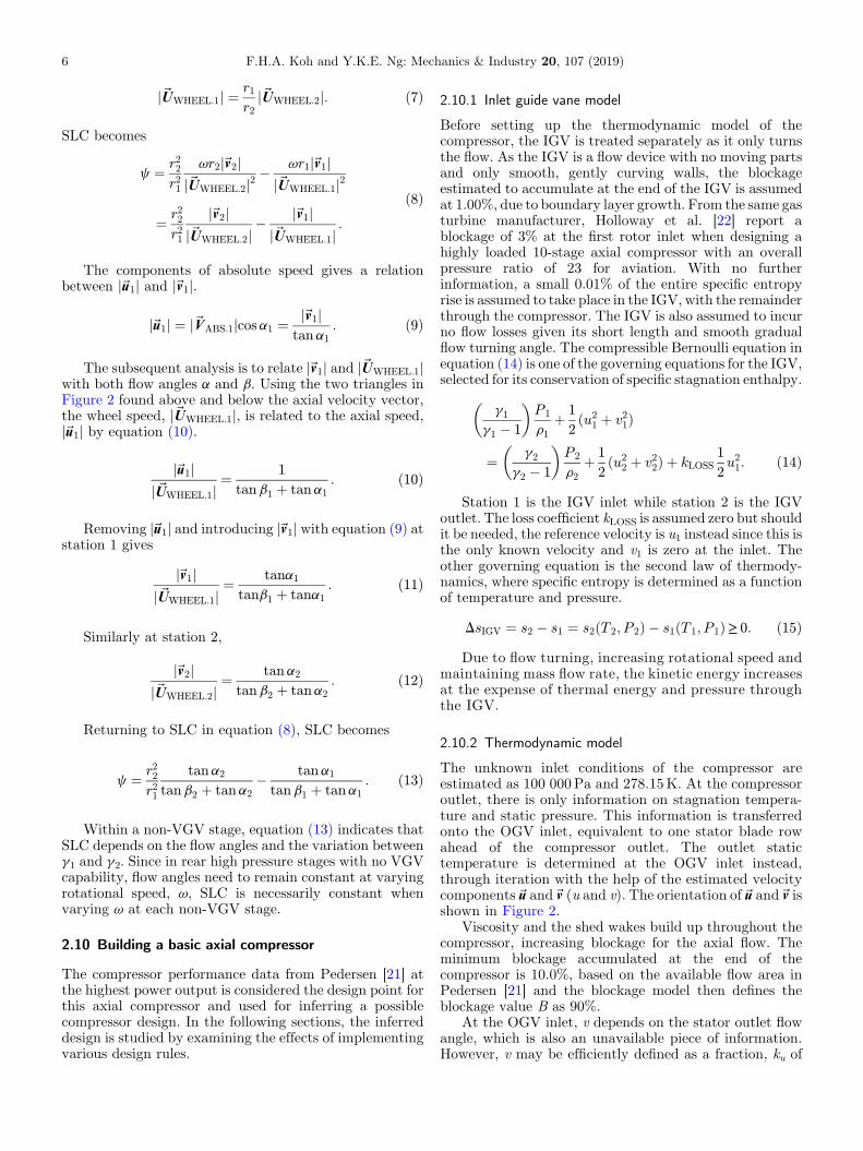
Fig. 2. Velocity diagram at the rotor inlet and rotor outlet.


design guideline is used to initialise the design process. Thisinitial design assumption results in similar flow angles atthe stage inlet and outlet. As the compressor designmatures, the stage inlet and outlet flow angles variationsare however allowed.

In the studied compressor, the axial velocity and thewheel speed are not constant throughout the compressor,implying varying velocity triangles. Wheel speed is aproduct of high pressure spool rotational speed and themean radius or Eulerian radius at each stage. Each stagehas been designed with a different Eulerian radius; hence,wheel speed is not constant. Attempting to obtain similarabsolute velocity and relative velocity flow angles at thestage inlet and outlet is too stringent. Among the manypossible departures from the RSRRdesign guide, this studyretained only the design rule of similar relative velocity flowangles at the stage inlet and outlet, until minor changes arenecessary to achieve a converged set of flow angles for allblades in all stages.

2.7 Iteration variables

Ready with all the inputs in the categories listed above,there are still two unknown flow angles that influence theflow speeds within the compressor. As the IGV flowturning angle is unknown, the absolute inlet flow angle ofthe first stage is also unknown. The other unknown angleis the absolute outlet flow angle at the last stage ofcompressor before the OGV, which is also referred to asthe absolute OGV inlet angle. These flow angles will be theiteration variables to explore the design space of flowangles for each stage. When a combination of IGV flowturning angle and absolute OGV inlet flow angle returns aset of flow angles, from all the stages, where the differencesbetween inlet velocity triangles and outlet velocitytriangles are acceptably small, this set of flow anglesand their corresponding flow speeds is considered aconverged solution of the SUSM.

2.8 Design guidelines for uncertain information

To reduce assuming a fixed value for uncertain informa-tion, the following minimum design guidelines areimplemented.
1. The axial flow speed, outer and inner radii are smooth
varying in the axial direction to reduce boundary layerbuild up.

2.
The stator and rotor blades are likely to have similarcamber angles at the initial design stage. Since flow ismore energetic across the rotor, the rotor blade isallowed more camber than the stator blade as thecalculation progresses.
3.
Stage reaction is initially assumed at 0.5 and is allowedto vary between 0.0 and 1.0.
4.
The de Haller number is calculated at each stage andchecked against the historical achievement of >0.72, asused in Falck’s [11] design approach. Saravanamuttooet al. [20] discusses the de Haller number as only aninitial design criterion. Due to the lack of more intimatemachinery details in this study, the de Haller number is
sufficient for the SUSM. The diffusion factor is a detaileddesign criterion requiring further compressor detailswhich may not be available.

5.
The inlet velocity triangle of a stage is very similar to theoutlet velocity triangle of the previous stage.
2.9 Stages without variable guide vanes

As greater compression takes place in the high pressurestages where there is typically no VGV, the SLC and flowangle relationship is examined next. At non-VGV stages,the angles of the velocity triangles at both the rotor inletand the rotor outlet need to be fairly consistent across arange of rotational speeds, v to achieve the intendedpressure rise. This implies at the inlet and outlet stationsof a blade row, the ratio of absolute speed VABS:relativespeed VREL:wheel speed UWHEEL in Figure 2 must remainsimilar to maintain velocity triangles of similar propor-tions when varying rotational speed.

The Euler whirl equation, eWHIRL is

eWHIRL ¼ DhTOT:STG ¼ vr2j~v2j � vr1j~v1j: ð3Þ

Combining the Euler whirl equation and SLC, c for anaxial stage gives

c ¼ DhTOT:STG

j~UWHEELj2¼ vr2j~v2j � vr1j~v1j

j~UWHEELj2: ð4Þ

Defining wheel speed j~UWHEELj at station 1 asj~UWHEEL:1j,

c ¼ vr2j~v2j � vr1j~v1jj~UWHEEL:1j2

¼ vr2j~v2jj~UWHEEL:1j2

� vr1j~v1jj~UWHEEL:1j2

: ð5Þ

Using the wheel speeds at stations 1 and 2, and notingthat v is common since the same shaft is used,

v ¼ j~UWHEEL:1jr1

¼ j~UWHEEL:2jr2

ð6Þ

a relationship between wheel speeds at different stations ofvarying radius is found


j~UWHEEL:1j ¼ r1r2

j~UWHEEL:2j: ð7Þ

SLC becomes

c ¼ r22r21

vr2j~v2jj~UWHEEL:2j2

� vr1j~v1jj~UWHEEL:1j2

¼ r22r21

j~v2jj~UWHEEL:2j

� j~v1jj~UWHEEL:1j

:

ð8Þ

The components of absolute speed gives a relationbetween j~u1j and j~v1j.

j~u1j ¼ j~VABS:1jcosa1 ¼ j~v1jtana1

: ð9Þ

The subsequent analysis is to relate j~v1j and j~UWHEEL:1jwith both flow angles a and b. Using the two triangles inFigure 2 found above and below the axial velocity vector,the wheel speed, j~UWHEEL:1j, is related to the axial speed,j~u1j by equation (10).

j~u1jj~UWHEEL:1j

¼ 1

tanb1 þ tana1: ð10Þ

Removing j~u1j and introducing j~v1j with equation (9) atstation 1 gives

j~v1jj~UWHEEL:1j

¼ tana1


Similarly at station 2,

j~v2jj~UWHEEL:2j

¼ tana2


Returning to SLC in equation (8), SLC becomes

c ¼ r22r21

tana2

tanb2 þ tana2� tana1


Within a non-VGV stage, equation (13) indicates thatSLC depends on the flow angles and the variation betweeng1 and g2. Since in rear high pressure stages with no VGVcapability, flow angles need to remain constant at varyingrotational speed, v, SLC is necessarily constant whenvarying v at each non-VGV stage.

2.10 Building a basic axial compressor

The compressor performance data from Pedersen [21] atthe highest power output is considered the design point forthis axial compressor and used for inferring a possiblecompressor design. In the following sections, the inferreddesign is studied by examining the effects of implementingvarious design rules.

2.10.1 Inlet guide vane model

Before setting up the thermodynamic model of thecompressor, the IGV is treated separately as it only turnsthe flow. As the IGV is a flow device with no moving partsand only smooth, gently curving walls, the blockageestimated to accumulate at the end of the IGV is assumedat 1.00%, due to boundary layer growth. From the same gasturbine manufacturer, Holloway et al. [22] report ablockage of 3% at the first rotor inlet when designing ahighly loaded 10-stage axial compressor with an overallpressure ratio of 23 for aviation. With no furtherinformation, a small 0.01% of the entire specific entropyrise is assumed to take place in the IGV, with the remainderthrough the compressor. The IGV is also assumed to incurno flow losses given its short length and smooth gradualflow turning angle. The compressible Bernoulli equation inequation (14) is one of the governing equations for the IGV,selected for its conservation of specific stagnation enthalpy.

g1g1 � 1

� �P 1

r1þ 1

2ðu2

1 þ v21Þ

¼ g2

g2 � 1

� �P2

r2þ 1

2ðu2

2 þ v22Þ þ kLOSS1

2u21: ð14Þ

Station 1 is the IGV inlet while station 2 is the IGVoutlet. The loss coefficient kLOSS is assumed zero but shouldit be needed, the reference velocity is u1 instead since this isthe only known velocity and v1 is zero at the inlet. Theother governing equation is the second law of thermody-namics, where specific entropy is determined as a functionof temperature and pressure.

DsIGV ¼ s2 � s1 ¼ s2ðT 2;P 2Þ � s1ðT 1;P 1Þ≥ 0: ð15ÞDue to flow turning, increasing rotational speed and

maintaining mass flow rate, the kinetic energy increasesat the expense of thermal energy and pressure throughthe IGV.

2.10.2 Thermodynamic model

The unknown inlet conditions of the compressor areestimated as 100 000Pa and 278.15K. At the compressoroutlet, there is only information on stagnation tempera-ture and static pressure. This information is transferredonto the OGV inlet, equivalent to one stator blade rowahead of the compressor outlet. The outlet statictemperature is determined at the OGV inlet instead,through iteration with the help of the estimated velocitycomponents~u and~v (u and v). The orientation of~u and~v isshown in Figure 2.

Viscosity and the shed wakes build up throughout thecompressor, increasing blockage for the axial flow. Theminimum blockage accumulated at the end of thecompressor is 10.0%, based on the available flow area inPedersen [21] and the blockage model then defines theblockage value B as 90%.

At the OGV inlet, v depends on the stator outlet flowangle, which is also an unavailable piece of information.However, v may be efficiently defined as a fraction, ku of


wheel speed from equation (16).

n ¼ kuvrE ð16Þwhere rE is the Eulerian radius at each blade row andrE ¼ ffiffiffiffiffiffiffiffiffiffiffiffiffiffiffiffiffiffiffiffiffiffiffiffiffiffiffiffiffiffiffiffiffiffiffiffiffiffiffiffiffiffiffiffi

0:5ðrCASE2 þ rCORE2Þp. The outlet static tempera-

ture T is found through the outlet stagnation temperature.With OGV inlet temperature and pressure determined, thespecific entropy rise in the whole compressor is calculated.

2.10.3 Stage loading coefficient model

In this SUSM, four possible SLC distribution models areconsidered. There is no preferred model as each gas turbinehas its unique heritage and possibly additional stages weredesigned differently as evident in the account by Smith [7]for a gas turbine manufacturer.
1. Constant SLC for non-VGV stages and constant SLC for
VGV stages: at each level of power output, the specificstagnation enthalpy rise through the compressor,DhTOT.COMP with corresponding rotational speed v isused in equation (17) to determine the SLC, c,distribution at that power level.

DhTOT:COMP ¼ cv2XSTGMAX

STG¼1

rE:STG2: ð17Þ

Using the set of data from Pedersen [13] with 11power output levels and thermodynamic data fromCengel [23], the third highest power output gives thelargest constant c at all stages. This is considered thedesign SLC, cDS.

2.
Constant temperature rise for all stages: based on thehighest power output, equation (18) gives the tempera-ture at each stage outlet. The velocity at the meanline fixes the specific stage stagnation enthalpy inequation (19) and in turn, determines the design SLC foreach stage, cDS,STG.
TSTG:OUT ¼ TCOMP:IN þ ðSTGÞ△TCOMP

STGMAXð18Þ

hTOT:STG:OUT ¼ hðT STG:OUTÞ þ 1

2ðuSTG2 þ vSTG2Þ: ð19Þ

This SLC model, which is based on constanttemperature rise through all stages, is inspired by aworked example in Mattingly [8], where a preliminarycompressor is designed without detailed stage tempera-ture information.

3.
Constant specific static enthalpy rise for all stages: usingthe operating point with the highest power output,equation (20) calculates the specific stagnation enthalpyat each stage outlet, which in turn determines the designSLC for each stage, cDS,STG.
hTOT:STG:OUT ¼ hCOMP:IN þ ðSTGÞ DhCOMP

ðSTGMAXÞþ 1

2ðuSTG2 þ vSTG2Þ: ð20Þ

The form of the SLC model based on constantspecific static enthalpy rise shares the same inspirationas the constant temperature rise SLC model andsupported by a rule of thumb for constant stage energyrise in [24]. Specific static enthalpy is the variable as thisis also common in turbomachinery analysis.

4.
Varying (decreasing) SLC across the stages: the SLCat the last stage is a percentage lower than the SLC atthe first stage, with SLC varying linearly across allthe middle stages. Using the operating point with thehighest power output, equation (21) gives the specificstage stagnation enthalpy rise in terms of the design SLCof each stage, cDS,STG. Using the specific stagnationenthalpy rise for the full compressor, equation (22)determines the design SLC of each stage.
DhTOT:STG ¼ cDS:STGðvrE:STGÞ2 ð21Þ

DhTOT:COMP ¼XSTGMAX

STG¼1

DhTOT:STG: ð22Þ

This decreasing SLC model was inspired by [25] wherethe front stages are deliberately highly loaded. Anincreasing SLC distribution may be possible too.

To determine the SLC distribution, the axial androtational components of the absolute velocity must beknown. However, these are found only after the velocitytriangle analysis. Therefore, a more comprehensivesolution requires iteration. To test the robustness of thesolution procedure, the SLC in equation (4) is approxi-mated by arguing that the specific stage stagnationenthalpy rise is similar to the specific stage static enthalpyrise, DhTOT.STG≈DhSTG and this removes the need toiterate as DhSTG may be determined without velocityinputs.

2.10.4 Pressure ratio model

In this SUSM, three possible pressure ratio models areavailable, each built with an efficiency model and a specificentropy model.
1. Pressure ratio guided by small stage polytropic efficiency
using reference specific entropy (function of temperature)
2. Pressure ratio guided by small stage polytropic
efficiency using specific entropy (function of temper-ature, pressure)

3.
Pressure ratio guided by fully isentropic compressionbased specific entropy (function of temperature, pres-sure)
Each pressure ratio model suggests a feasible relativedistribution of maximum stage pressure ratios for all thestages. There is no best model as pressure ratio isdetermined stage by stage to meet the overall pressureratio, which in turn fulfills several possible objectives. Thegas turbine could have been designed for maximum overallpressure ratio or the most economical maintenancepackage. An inference using the overall pressure ratio isat best an estimate and cannot compensate for unavailableinformation, considering that an actual design has as manyas a million details as pointed out by Ghisu et al. [2].

Fig. 3. Blockage models in this study.


In pressure ratio model 1, the actual specific stageentropy rise is not known beforehand. However, the stageefficiency may be approximated by the compressor’spolytropic efficiency (23), with a mean g,g determined fromthe conditions at the inlet and outlet of the compressor.

nSTG � h2S � h1

h2 � h1� nPOLY � g � 1

gln�p2=p1�

ln{�1=h��P 2=P1��g � 1�=g � 1� � 1}: �23�

The specific stage outlet static enthalpy, h2 and thespecific stage isentropic outlet static enthalpy, h2s lie on thesame isobar on the h–s diagram, experiencing the samepressure rise. To avoid the still unknown actual specificstage entropy rise, isentropic compression calculationis carried out with h2s. The specific entropy rise inequation (24) is set to zero and usingT2s=T(h2s), a feasiblestage pressure ratio is estimated from P2/P1.

DsSTG ¼ S0ðT 2SÞ � S0ðT 1Þ �R lnP 2

P 1¼ 0: ð24Þ

The specific reference entropy s0 is from the thermody-namic table for air from Cengel [23].

Pressure ratio model 2 is similar to pressure ratiomodel 1 except specific entropy is a function oftemperature and pressure based on the s–T–P chart byAartun [26]. Using the stage inlet temperature, T1 and thestage isentropic outlet temperature, T2S the specificentropy rise in equation (25) determines the stage pressureratio, P2/P1.

DSSTG ¼ sðT 2S;P 2Þ � sðT 1;P 1Þ ¼ 0: ð25ÞIn pressure ratio model 3, knowing that for a given

temperature rise,T1–T2, the maximum pressure rise occurswhen the specific entropy rise is zero. With available inletand outlet temperatures from the selected SLC model,specific entropy is found as a function of temperature andpressure based on the s–T–P chart by Aartun [26].Equation (26) determines the maximum stage pressureratio, P1/P2.

DSSTG ¼ sðT 2;P 2Þ � sðT 1;P1Þ ¼ 0: ð26Þ

The actual stage pressure ratio is lower than maximumstagepressure ratio, and in thisway, accounts for the specificstage entropy rise. The specific stage entropy rise isproportional to the maximum pressure rise in a stage forthe same stage efficiency and assuming nearly linear isobarson the T–s diagram. In this way, the stage losses aredistributed according to the stage compression capability.The lower actual pressure ratio is also determined in such away that a smooth axial velocity distribution results at thefront of the compressor. All stages are subjected to the samefraction except thefirst stage. In the studied compressor, thesame fraction kPR is applied on stages 2 to 16 and kPR,1 forstage 1. The iteration variable is kPR. Each guessed kPR isautomatically constrained by equation (27) such that allstage pressure ratios achieve the overall pressure ratio of thecompressor, OPR as kPR,1 takes the slack.

OPR ¼ PRACT:1 ∏STGMAX

STG¼2

PRACT:STG ð27Þ

where PRACT:STG ¼ KPRPRMOD:STG and PRACT:1 ¼ kPR:1PRMOD:1.

Next, the stage temperature, gas law andmass flow rateconservation determine the no-blockage axial velocity ateach stage outlet. Iteration continues till the no-blockagevelocity distribution from stage 1 to stage 3 varies linearlywith compressor axial coordinate x, in a straight line fit of3 points. The no-blockage velocity was selected as itdepends only on geometry since the boundary layer buildup is assumed small at the beginning of the compressor.

2.10.5 Blockage model

Blockage in a gas turbine compressor is challenging todefine accurately due to the accumulation of wakes frommultiple bodies interrupting the flow. Falck’s [11] LUAX-Cdesign code suggests that the blockage increases at 0.5%per stage and stabilises after stage 8. This idea was adaptedto give blockage models 1 and 2 in Figure 3. The finalblockage was set to 10% for both a smooth and abrupttransition at about stage 8. The data from Pedersen [21]indicates that the maximum available flow area throughthe compressor follows a steep “s” shaped curve and reachesa steady level of 90% availability in cross-section area in thelast few stages of the compressor and is designated asblockage model 3 in Figure 3.

2.10.6 Velocity triangle model

The velocity triangles of the last stage of this compressorare determined first since at the outlet of the last stage, allthe flow quantities are known. Based on the analysis of non-VGV stages in Section 2.9, non-VGV stages require similarvelocity triangles which in turn need similar SLC. Solvingfrom the last stage to the first stage results in more similarflow angles in the last stages as departures from the RSRRdesign guide are admitted only at the front stages. Thisapproach is found to ease solution convergence difficulties.

For each stage, the solution is a set of blade angles andflow angles where the Euler whirl matches the specificstagnation enthalpy rise, where the de Haller number is


met for both rotor and stator and the stage reaction isreasonable. The stage reaction is initially 0.5 and allowed tovary as iteration proceeds. The rotor blade is given morecurvature than the stator blade as the solution iterates.

At each stage, the solution process begins at the stageoutlet, where specific stagnation enthalpy, the flowvelocities, blade angles and thermodynamic propertiesare found. Moving to the stage inlet, this SUSM appliesonly initially the design rule of similar relative velocity flowangles at the stage inlet and outlet, b1=b3. The b1 angleenables determining the stage inlet flow angles, bladeangles and thermodynamic properties. The rotor-statorinterface quantities in the middle of the stage aredetermined by degree of reaction, RREAT in equation (28),

h2 ¼ h1 þRREACTðh3 � h1Þ ð28Þand conservation of specific stagnation enthalpy acrossstator in equation (29). This sets up the specific staticenthalpy and specific stagnation enthalpy to determine theabsolute velocity.

hTOT:2 ¼ hTOT:3: ð29ÞUsing the absolute velocity, the rotor–stator interfaceblade angles and thermodynamic properties are found.With all flow angles and thermodynamic propertiesavailable, the stage Euler whirl in equation (3) is the“hard” criteria used to test the suitability of stage reactionand inlet relative velocity angle. The first “soft” criterion isthe stage degree of reaction, which ranges about 0.5 forthe axial compressor in this study. The next “soft” criteriaare the difference in blade angles, Du from blade angles,uROT ¼ b2 � b1 and uSTA ¼ a3 � a2.

Du ¼ uROT � uSTA: ð30ÞThe de Haller number, dH is the last “soft” criteria,

which is a ratio of relative outlet speed to relative inletspeed for the rotor blades and absolute outlet speed toabsolute inlet speed for the stator blades.

dℋROT ¼ V REL:2=V REL:1

dℋSTA ¼ V ABS:3=V ABS:2:ð31Þ

Since there is insufficient design information to allow adirect calculation of the flow and blade angles, a suitablerange of values are accepted for the design variables,RREACT, Du are dℋ, according to the design guidelines foruncertain information in Section 2. Being a “hard” criteria,Euler whirl, eWHIRL is used in an error variable eHARD inequation (32) to iteratively suggest a Du that results in anEuler whirl which matches the specific stage stagnationenthalpy rise.

eHARD ¼ eWHIRL � ðhTOT:3 � hTOT:1ÞhTOT3 � hTOT:1

: ð32Þ

Consequently, the stage degree of reaction is alsoaffected and is updated with another error variable eSOFT inequation (33).

eSOFT ¼ uROT � ðuSTA þ DuÞuSTA þ Du

: ð33Þ

When the stage degree of reaction and acceptable angledifference Du between the rotor and stator blade angles donot result in feasible set of blade and flow angles, the inletrelative flow angle b1 is adjusted with the eHARD errorvariable. The design variables VDS are updated with theirerror variables e and a relaxation factor, fRELAX to preventover-correction, according to equation (34).

V DS:NEW ¼ V DS:OLDð1± fRELAXeÞ ð34Þwhere the subscripts “NEW” and “OLD” refer to theupdated and previous values, respectively.

3 Results

A basic axial compressor from Section 2.10 is “designed”with the following inputs to study the influence of the IGVflow turning angle, the OGV inlet angle, the pressure ratiomodels and the SLC models. The SLC is constant for thenon-VGV stages and also constant SLC for the VGVstages (SLC model 1). The distribution of stage pressureratios is based on fully isentropic compression usingspecific entropy as a function of temperature and pressureapplied to each stage (pressure ratio model 3). Theblockage from boundary layer shedding off the blades aswakes and stationary wall boundary layers is set to growto a maximum of 10% of the cross-sectional area, usingblockage model 1. The “design” goal is to reduce the meanamount of mismatch in flow angles at the stage-outlet–stage-inlet interfaces. The simplified solution procedure,where, the specific stage stagnation enthalpy rise isassumed similar to the specific stage static enthalpyrise, DhTOT:STG ≈DhSTG is used to remove the need toiterate, sacrificing improved results for speed.

Using the stage un-stacking approach in Section 2, alarge collection of data is generated for a range of IGVflowing turn angles and OGV inlet flow angles (before theOGV straightens the flow), to locate the design space wherethe mismatches in flow angles at each stage interface isminimal. This would indicate a possible axial compressordesign at the operating point.

3.1 Effect of increasing IGV flowing turn angle

To study the effect of increasing the IGV flow turningangle, Figure 4 shows the data generated for IGV flowingturn angles from 20° to 34° and for selected rotationalcomponents of the absolute velocity at the OGV inlet. Therotational component v is a fraction, varying from0.42 to 0.52, of the OGV inlet wheel speed, defined inequation (16). Each data point represents a set of designchoices that results in a feasible set of flow angles for thewhole compressor.

As both the IGV flow turning angle and v, the fractionof wheel speed, increase towards the optimum combinationof IGV flow turning angle of about 31° and v close to 0.46 of

Fig. 4. The effect of flow turning angle in the IGV on the mean mismatch in flow angles per stage at each stator-outlet–rotor-inletinterface.


the OGV inlet wheel speed, it becomes possible to obtain aset of feasible flow turning angles for the axial compressoras a whole that achieves minimal mismatch in flow anglesat each stator-outlet–rotor-inlet interface between stages.However, as the fraction of wheel speed increases further, itagain becomes increasingly difficult to obtain a set offeasible flow turning angles for the whole compressor. Sincethe axial compressor’s design is highly optimized, the manydesign parameters simultaneously match narrowly onlyabout the design point.

3.2 Effect of OGV inlet flow angles

The velocity components u and v at the OGV inletdetermine the outlet flow angle at the last stage’s stator.An improved estimate of the specific stagnation

enthalpy at the OGV inlet requires the rotationalcomponent v before allocating sufficient specific staticand stagnation enthalpy to each axial compressor stage.Using the same generated data for IGV flow turningangles, the effect of OGV inlet flow angle is examined byvarying v and presented in Figure 5. Each data point inFigure 5 represents a set of design choices that results infeasible set of flow angles across the whole compressor.For clarity, only the even IGV flow turning angles areshown.

Increasing v as a fraction of wheel speed at the outlethas only a small effect on reducing the amount of mismatchin flow angles at the stator-outlet–rotor-inlet interface.Adjustments to v hardly minimise the flow anglemismatches unless the IGV flow turning angle is close to31° for this axial compressor.

Fig. 5. The effect of increasing v as a fraction of wheel speed atthe OGV inlet on the mean mismatch in flow angles per stage ateach stator-outlet–rotor-inlet interface.

Fig. 6. Comparison ofmean flow anglemismatch between pressureratio models.


3.3 Effect of pressure ratio model

The effects of different pressure ratio models on an axialcompressor’s flow angles at the design point are examinedwith a basic compressor from Section 2.10, where the IGVflow turning angle is 28° and at the OGV inlet, v=0.45of the wheel speed. The SLC model 1 sets the axialtemperature distribution, assuming DhTOT:STG ≈DhSTG.The combined effect of the choice of pressure ratio modeland the method that smooths the velocity distributionhas minimal effect on the mean flow angle mismatch atthe stator-outlet–rotor-inlet interfaces as seen in Figure 6.The pressure ratio models only distribute availablepressure among the stages of the axial compressor. Withinthe overall compression ratio of this axial compressor, anyadditional rise in pressure ratio in a stage is compensatedwith a lower pressure ratio in another stage. For example,the lower pressure ratios at the rear stages suggestedby pressure ratio model 3 are complemented by higherpressure ratios in the front stages and the reverse occurspressure ratio models 1 in Figure 7B.

The choice of pressure ratio model, however, does affectthe maximum pressure ratio available at each stage as seenin Figure 7A, where pressure ratio model 3 delivers morecompression in the front stages compared to pressure ratiomodel 1 and 2. This effect is present in a small way in theactual stage pressure ratios in Figure 7B. The estimated

stage pressure ratio is closer to the actual from only stage 5onwards. The “PR GE LM2500” data in Figure 7B is takenfrom Klapproth et al. [15].

The resulting axial velocity profile in Figure 8 is smoothat the front stages even after factoring the effect ofblockage. However, when moving from the last VGV stageto first non-VGV stage, there is a rougher transition. Thiswould happen as this SUSM has no provision for transitingthe flow from a VGV stage to a non-VGV stage. For thesame mass flow rate, the axial velocity distribution frompressure ratio model 3 in Figure 8 does indicate lower axialvelocities, implying higher density from higher pressureratios in the front stages.

Considering that the actual axial velocity distribu-tion (“Act. Ax. Vel.” in Fig. 8) from Klapproth et al. [15]is not always smooth, the rough transition in axialvelocity is acceptable. According to the approximatecompressor schematic on the gas turbine manufacturer’smarketing datasheet [14], there is a proportionally longerstator at stage 8. The 8th stage stator houses the bleedair valve, according to Klapproth et al. [15]. In the non-VGV stages, the axial speeds show the greatestdifference. This difference is traced to several possiblesources, the OGV, bleed air, annulus cross-sectional areaand blockage.

The OGV is mentioned by Klapproth et al. [15] butthere is too little information on the cross-sectional areaand the axial length for a proper analysis of the flow speed.Should theOGVbe part of the analysis, it would contributeonly a small pressure rise. The OGVwould only verymildlyreduce the stage loading at all stages as a small pressureand temperature rise is obtained through straightening theflow. The corresponding mild reduction in stage compres-sion would give lower stage density at the last stages andthe axial speeds would increase to maintain the same massflow rate. Therefore, the OGV excluded from the analysis isnot a cause of higher axial flow speed at the last stages. Inaddition, inferring the radius from the same approximatecompressor schematic on the gas turbine manufacturer’smarketing datasheet [14], there is little change in cross-sectional area after the last compressor stage, implyingaxial mass flux might keep constant after flow straighten-ing. Since pressure increases to give higher density throughthe OGV, lower axial speed results after the OGV tomaintain mass flow rate. This would not affect the axialspeeds of the last compressor stages. Bleed air for filmcooling in the high pressure turbine is interpreted asobtained from the compressor discharge according to thetechnical section of this 3rd party market analysis [27], anddoes not affect the axial speed at the last stages. Similarno-blockage annulus cross-sectional area is found byestimating the radius from the same approximate com-pressor schematic on the manufacturer’s marketing data-sheet [14] and using data in Pedersen [13]. The estimatedradius from the same approximate compressor schematicon the manufacturer’s marketing datasheet [14] results in aslightly larger annulus cross-sectional area. The blockagemodel supported by data in Pedersen [21] shows a clear10% reduction in available cross-sectional area after stage 9as indicated in Figure 3. This level of blockage is used at theOGV inlet. To resolve this obvious difference in axial speed

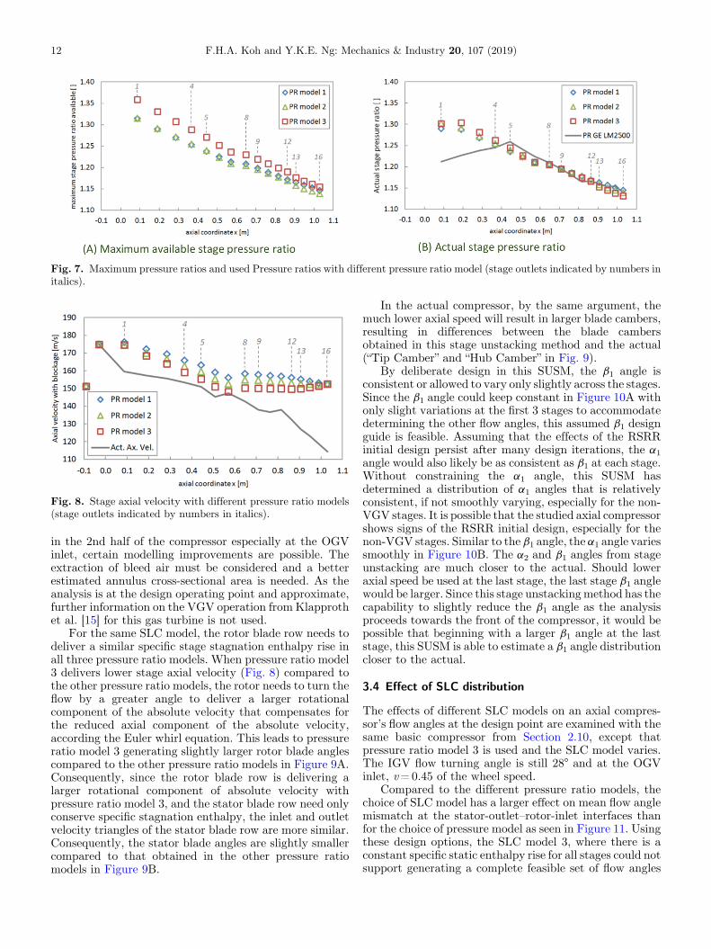
Fig. 8. Stage axial velocity with different pressure ratio models(stage outlets indicated by numbers in italics).

Fig. 7. Maximum pressure ratios and used Pressure ratios with different pressure ratio model (stage outlets indicated by numbers initalics).


in the 2nd half of the compressor especially at the OGVinlet, certain modelling improvements are possible. Theextraction of bleed air must be considered and a betterestimated annulus cross-sectional area is needed. As theanalysis is at the design operating point and approximate,further information on the VGV operation from Klapprothet al. [15] for this gas turbine is not used.

For the same SLC model, the rotor blade row needs todeliver a similar specific stage stagnation enthalpy rise inall three pressure ratio models. When pressure ratio model3 delivers lower stage axial velocity (Fig. 8) compared tothe other pressure ratio models, the rotor needs to turn theflow by a greater angle to deliver a larger rotationalcomponent of the absolute velocity that compensates forthe reduced axial component of the absolute velocity,according the Euler whirl equation. This leads to pressureratio model 3 generating slightly larger rotor blade anglescompared to the other pressure ratio models in Figure 9A.Consequently, since the rotor blade row is delivering alarger rotational component of absolute velocity withpressure ratio model 3, and the stator blade row need onlyconserve specific stagnation enthalpy, the inlet and outletvelocity triangles of the stator blade row are more similar.Consequently, the stator blade angles are slightly smallercompared to that obtained in the other pressure ratiomodels in Figure 9B.

In the actual compressor, by the same argument, themuch lower axial speed will result in larger blade cambers,resulting in differences between the blade cambersobtained in this stage unstacking method and the actual(“Tip Camber” and “Hub Camber” in Fig. 9).

By deliberate design in this SUSM, the b1 angle isconsistent or allowed to vary only slightly across the stages.Since the b1 angle could keep constant in Figure 10A withonly slight variations at the first 3 stages to accommodatedetermining the other flow angles, this assumed b1 designguide is feasible. Assuming that the effects of the RSRRinitial design persist after many design iterations, the a1angle would also likely be as consistent as b1 at each stage.Without constraining the a1 angle, this SUSM hasdetermined a distribution of a1 angles that is relativelyconsistent, if not smoothly varying, especially for the non-VGV stages. It is possible that the studied axial compressorshows signs of the RSRR initial design, especially for thenon-VGV stages. Similar to the b1 angle, the a1 angle variessmoothly in Figure 10B. The a2 and b1 angles from stageunstacking are much closer to the actual. Should loweraxial speed be used at the last stage, the last stage b1 anglewould be larger. Since this stage unstackingmethod has thecapability to slightly reduce the b1 angle as the analysisproceeds towards the front of the compressor, it would bepossible that beginning with a larger b1 angle at the laststage, this SUSM is able to estimate a b1 angle distributioncloser to the actual.

3.4 Effect of SLC distribution

The effects of different SLC models on an axial compres-sor’s flow angles at the design point are examined with thesame basic compressor from Section 2.10, except thatpressure ratio model 3 is used and the SLC model varies.The IGV flow turning angle is still 28° and at the OGVinlet, v=0.45 of the wheel speed.

Compared to the different pressure ratio models, thechoice of SLC model has a larger effect on mean flow anglemismatch at the stator-outlet–rotor-inlet interfaces thanfor the choice of pressure model as seen in Figure 11. Usingthese design options, the SLC model 3, where there is aconstant specific static enthalpy rise for all stages could notsupport generating a complete feasible set of flow angles

Fig. 10. Flow angles with different pressure ratio models.

Fig. 9. Blade angles with different pressure ratio models.

Fig. 11. Comparison of mean flow angle mismatch between SLCmodels.


that fit all stages. While generating the velocity trianglesfrom the OGV inlet to the inlet with SLC model 3, theavailable energy and requirements could not set up aproper velocity triangle at a middle stage within this axialcompressor.

The stage SLC distribution in Figure 12 shows thatmodel 3 with constant specific stage static enthalpy rise hasthe lowest SLCs for the non-VGV stages. The compressordesigned with SLC model 3 imparts lesser specificstagnation enthalpy to the working fluid when higherrotational kinetic energy (vrE) is available at the rear

stages. At the same time, the front stages must imparthigher specific stagnation enthalpy to the working fluidwhen lesser rotational kinetic is available as the Eulerianradius, rE is smaller.

The specific stage static enthalpy rise in Figure 13shows the same trend as stage SLC since the simplifyingassumption that DhTOT:STG ≈DhSTG is used in the SLCdefinition. Because SLC model 3 could not support infinding a complete set of flow angles for the whole axialcompressor, the specific stage static enthalpy distributionsin SLC models 1, 2 and 4 indicate that specific stage staticenthalpy rise must increase stage after stage for thisaxial compressor. The specific stage static enthalpy rise inmodel 2 is not a smooth curve as the temperature-specificstatic enthalpy function is only sufficiently piecewise smooth.

In this SUSM, the stage pressure ratios cannot be fixedwhile varying the stage load coefficient because only thevariation in pressure ratios is available for smoothing theaxial velocity especially from the IGV to the 2nd stage ofthe axial compressor. However, the difference is stagepressure ratios in Figure 14 are small from stage 5 onwards.The major difference is found in stages 1–4, where higherspecific static enthalpy rises (Fig. 13) correspond to higherpressure ratios (Fig. 14).

Since the compressor inlet axial speed is known, eachSLC model works with the same pressure ratio model togenerate the same inlet density, resulting in pressure andtemperature moving in tandem at the inlet. In thesubsequent stages, for the same mass flow rate and known

Fig. 12. Stage SLC distribution with different SLC models.

Fig. 13. Specific stage static enthalpy rise with different SLCmodels.

Fig. 14. Stage pressure ratios with different SLC models.

Fig. 15. Stage axial velocity with different SLC models.


smooth cross-sectional area variation, a smooth densityvariation is needed to generate a smooth axial velocityprofile. This smooth density variation further maintainsthe differences in pressure ratio for the front few stages.

By the 2nd stage in the axial compressor, Figure 15shows that the axial velocity is no longer influenced by theconditions at the compressor inlet. In SLC model 1, due tothe initial lower pressure ratios, the resulting lower densityflow is compensated by increasing the axial velocitythrough the rest of the axial compressor. The oppositeoccurs for SLC model 3, which has the highest initialcompression of the 4 SLC models.

4 Discussion

This SUSM is applied to the design operating point only.The actively adjustable design options are the choice ofSLC model, pressure ratio model, blockage model andamount of blockage. These factors work through themethod to determine the overall specific stage staticenthalpy rise, stage pressure ratios and axial velocityprofile through the axial compressor. These in turndetermine velocities and flow angles within each stage ofthe axial compressor, which in turn determine the amountof flow angle mismatch.

4.1 IGV flow turning angle

While the implemented design options have identified adesign space where a range of inputs are able to generatezero flow angle mismatches between the stages, the mostinfluential design option that reduces angle mismatches tozero is the IGV flow turning angle.

In terms of reducing the mean mismatches in flowangles per stage, varying the OGV inlet flow angle byvarying v as a fraction of wheel speed at the OGV inletexerts little influence. In this LM2500 compressor,increasing v causes no increase in OGV inlet specificstagnation enthalpy since the compressor’s outlet stagna-tion temperature is fixed. However, increasing v reduces thespecific static enthalpy only slightly as the velocitycontribution to specific stagnation enthalpy is small. A10% increase in v from 42% to 52% of wheel speed at theOGV inlet results in only about 0.05 kJ/kg change inspecific stagnation enthalpy at the stage before the OGVinlet. Furthermore, beyond this small 10% range of v, thereare either no feasible sets of flow angles for the wholecompressor or the flow angle mismatch cannot reach zero.

In contrast, adjusting the IGV flow turning angle exertsa greater influence on reducing the mean mismatches inflow angles per stage. For solutions surrounding theoptimum IGV flow turning angle that results in zero flowanglemismatches across all stages, a 1° increase in IGV flow

Fig. 16. Pressure ratio distribution of selected gas turbines.


turning angle causes a 0.2–0.5 kJ/kg specific staticenthalpy drop at the IGV outlet. For a more quantitativecomparison, a 3° change about the optimum IGV flowturning angle of about 31° (≈10% change) causes about0.6–1.5 kJ/kg change in specific stagnation enthalpy, at theIGV outlet (stage 1 inlet), which is easily 10 times greaterthan the specific static enthalpy changes implemented atthe OGV inlet.

Determining matching flow angles between stages andfor the Euler whirl to match the specific stagnationenthalpy rise at each stage for all 16 stages of thiscompressor is akin to simultaneously satisfying 32 sets ofrequirements. These requirements and the compressor’soverall pressure and temperature ratios are thereforeactually coupled together to characterize the design of thestudied axial compressor. This large number of constraintsnaturally greatly narrows the solution range of both theIGV flow turning angle to near 31° and v to about 0.46 ofthe OGV inlet wheel speed for this axial compressor.However, as v at theOGV inlet hasmuch lesser influence onflow anglemismatches than the IGV flow turning angle, theangle mismatches are efficiently first reduced by adjustingthe IGV flow turning angle and if needed, followed by finetuning with v at the OGV inlet.

4.2 Pressure ratio distribution

Smith [7] documents the rich design heritage of this gasturbine which has experienced 2 rounds of stage additionsat the rear. While there is little doubt of an improvedunderstanding of the underlying physics of flow and ofmaterials, the account by Smith [7], shows instead that theproven aspects of the current design are retained in theinterest of reliability when addingmore stages.Wadia et al.[16] report the most recent addition of the 0th stage to thefront of the compressor where little of the original gasturbine is altered. This implies that the design approach ispossibly not consistent in all aspects across the compressor.In Figure 16, the shape of the pressure ratio distributioncurve of the studied compressor is compared to anothercompressor by the same manufacturer “PR GE NASAEEE” referred to by Bruna et al. [28] and a similar 17 stagemachine (PR Hitachi 17 stg) by Kashiwabara et al. [25].The inlet is 0 and the compressor outlet is 1 on thehorizontal axis.

The GE LM2500 and Hitachi 17-stage are land basedturbines. In the design of the Hitachi 17-stage compressor,the front 3 stages are highly loaded [25]. The GE LM2500compressor does not deliberately load the front stages.While the design perspectives differ, the stage pressureratio distributions are similar with a peak in pressure ratioat one of the front stages. The “GE NASA EEE” refers tothe Energy Efficient Engine (EEE) and is meant tosupport aviation engine development. The detailed designphase of compressor of the “GE NASA EEE” began withspecifying the specific stagnation temperature rise at eachstage for the design operating point seen in Figure 14 fromHolloway et al. [22]. This distribution was overalldecreasing with stage number except the middle stages6 and 7, where the decrease was more obvious. The initialdistribution of the stage static temperature rise inFigure 27 from Holloway et al. [22] is similar. In the finalconfiguration, the static temperature distribution throughthe stages did not change too much as seen also inFigure 27 from Holloway et al. [22]. While the “GE NASAEEE” pressure ratio was not specified directly, itsynchronizes closely with the temperature variation.Therefore, the distribution of stage pressure ratio is adesign choice, driven by temperature variation andtherefore SLC.

These 3 designs show that aggressive compression in theearly stages is more feasible than in the later stages. Theimportant detail is which stage then delivers the highestpressure ratio. The absolute pressure rise of the first stagein the EEE would be smaller than that of the other twocompressors, since the EEE design operates primarily in alow ambient pressure environment of 22 631.264Pa at11 km altitude according to Frei’s [29] online atmosphericpressure calculator. However, more pressure ratio distri-butions from actual compressors are needed before a firmdesign guideline may be constructed.

The pressure ratio models, and their supporting SLCmodels, suggested so far are suited only for preliminaryanalysis. The difference between the shapes of the pressureratio distribution curves estimated in Figure 7B and theactual in Figure 16 can only be resolved with a morecomprehensive SLC distribution. For this LM2500 com-pressor, the axial temperature distribution is not available.This impedes inferring the actual SLC distribution. A clearimprovement to this SUSM is in the SLC models. A morerealistic SLC distribution inferred for the LM2500compressor is shown in Figure 17 and this is based onthe stage pressure ratios in Figure 16. This distributioncontains details that presented simpler SLC models do nothave, hence the differences between the estimated andactual stage pressure ratios.

4.3 Acceptable range for camber angles

In a worked example in Mattingly [8], the RSRR approachis applied to stage stack an axial compressor, generating alarge database of possible values for the design variables.The difference between the inlet and outlet flow angles of ablade row ranged from 7° to 30°. For an NACA 65, a=1.0series airfoil, this translates to a camber of 1.53% to 6.58%of the chord where the camber lines are circular arcs.

ig 17. Estimated SLC distribution for the compressor in theM 2500 gas turbine.


FL

Table 1. Span wise radial mean blade curvature angles.

Experiment Blade row Spanwise(radial direction)mean bladecamber angle

Test CaseE/CO-1

Rotor 51.81°

Test CaseE/CO-3

Rotor 17.27°

Stator 47.30°Test CaseE/CO-5

Rotor for stage 1 and 2 38.36°

Stator for stage 1 and 2 43.78°

Noting that incidence angles and deviation angle areusually small at the design operating point, the estimatedblade angles from this SUSM are well within this range.

While solving for the stage flow angles, a stage with arelatively higher stage axial velocity makes for less,therefore easier, rotational velocity contributions tospecific stagnation enthalpy, which in turns requires lessflow turning in the rotor blade row. This eventually lowersthe blade curvature and consequently also lowers thetendency for boundary layer growth and separation on thesuction surface.

The flow features surrounding the blades are describedin relatively greater detail in Test Case E/CO-1 by Serovyand Dring [30], Test Case E/CO-3 by Ginder and Harris[31] and Test Case E/CO-5 by Serovy andDring [32] for thepurpose of bench marking computational fluid dynamicscodes. The blade curvature angles used in the blade rows ofthe three relevant test cases are calculated across the spanin the radial direction and shown in Table 1. The estimatedblade angles from this SUSMare also well within this range.

4.4 Selected stage loading coefficient and pressureratio models

The pressure ratio distribution of the LM2500 spans arelatively small range indicating that the loading on each

stage appears similar. Currently, SLC Model 1 representsthis best. For the same SLC distribution, the pressure ratiomodel 1 gives a slightly more balanced distribution acrossall stages. The blockagemodel is 1. However, this suggestedSLC distribution is more appropriately considered aninitial well-informed estimate.

5 Conclusion

This paper presents an SUSM that determines thevelocities and flow angles within a multistage axialcompressor. The design options in this method are builtupon inferred possible design guidelines implemented inactual gas turbines. The design options are implemented infour SLC models, three pressure ratio models and threeblockage models which, working with other requiredinformation, determines the stage velocities and stage flowangles for an axial compressor operating at design point.The method implements a calculation procedure thatsimultaneously fulfills thermodynamic requirements, ve-locity triangle requirements and user-selected designoptions for the whole axial compressor at the mean line.The outputs are specific static enthalpy, pressure, axialvelocity and flow angles at each stage interface of the axialcompressor. The SUSM is tested with a set of operationdata from an actual aero-derivative gas turbine. Throughadjusting of the IGV flow turning angle and OGV inlet flowangle, the method identifies a small range of design optionsthat suggests an axial compressor with minimal mismatchof flow angle at each stage interface. Among the adjustabledesign options, the method shows that the IGV flowturning angle has the most influence on minimising flowangle mismatches compared to the other design options.

Nomenclatures

Uppercase

A
Station cross sectional area (m2) B Blockage in terms of fraction of available station
cross sectional area for flow (dimensionless)
D Diffusion factor, a measure of the blade loading
(dimensionless)
J Mechanical equivalent of heat, 778.2 ft-lb/Btu
or 1 J/J where 1 ft-lb= 1.35582 J and 1 Btu=1055.06 J (dimensionless)

OPR
Overall pressure ratio of the compressor (di-mensionless)
P
Absolute pressure in Pascal (Pa) PRMOD Stage pressure ratio determined from the
pressure ratio models (dimensionless)
PRACT Actual stage pressure ratio used (dimensionless) R Gas constant for air (J/kg.K) RREACT Stage degree of reaction (dimensionless) c The stage load coefficient (dimensionless) cDS The design SLC, which could be a single value for
all stages or a distribution of values by stage(dimensionless)


T
Absolute temperature in Kelvins (K) U~WHEEL The rotor tangential speed, also referred to as
wheel speed UWHEEL (m s�1)
V~ABS The absolute velocity in the velocity triangles for
turbo-machinery analysis and also referred to asVABS (m s�1)

V~REL
The free stream velocity outside the boundarylayer, which is the velocity relative to the bladeand is the relative velocity in the velocitytriangle analysis for turbo-machinery and alsoreferred to as VREL (m s�1)
V~DS
The general symbol for a design variable(depends on variable)
Lowercase

CP
Specific heat of air at constant pressure (J/kg.K) CV Specific heat of air at constant volume (J/kg.K) eWHIRL Euler whirl (J/kg) fRELAX The general symbol for a relaxation factor
(dimensionless)
h Specific enthalpy (J/kg) kLOSS The coefficient of loss for flow in the Bernoulli
equation (dimensionless)
KPR Actual fraction of the stage pressure ratio found
in the pressure ratio models (dimensionless)
KPR.1 The KPR for stage 1 of the compressor (dimen-
sionless)
Ku The fraction of wheel speed at the OGV inlet
(dimensionless)
m The mass flow rate (kg/s) gCASE Casing radius (m) rCORE Hub radius (m) gE Eulerian radius (m) S Specific entropy (J/kg.K) SO Specific reference entropy from thermodynamic
tables (J/kg.K)
~u or u The axial component of V ABS also referred to as u
(m s�1)
~V or V The tangential component of V ABS also referred
to as V~(m s�1)
x Axial coordinate of the compressor (m)
Greek

a
The flow angle of the V ABS makes with the axialdirection in velocity triangle analysis for turbo-machinery (°)
b
The flow angle of the V REL makes with the axialdirection in velocity triangle analysis for turbo-machinery (°)
g
The ratio of specific heats, CP/CV (dimensionless) g Mean ratio of specific heats between two or more
stations in the compressor (dimensionless)
∊ The general symbol for an error variable (dimen-
sionless)
n Thermodynamic efficiency (dimensionless) uROT The angle of the curvature of the rotor blade (°) uSTA The angle of the curvature of the stator blade (°) Du The difference in angle of curvature of the rotor and
stator blade (°)

r
Density of the working gas which is air in this study(kg/m3)
s
Blade solidity which is the ratio of chord to pitch(dimensionless)
v
Shaft rotational speed (rad/s)
Script

dℋ
The de Haller number (dimensionless)
Subscript

1
The blade leading edge which is also considered tobe equivalent to the upstream measuring stationof the blade row or blade row inlet station
2
The blade trailing edge which is considered to beequivalent to the downstream measuring stationof the blade row or blade row outlet station
ABS
Absolute CASE The compressor casing CFD Computational fluid dynamics COMP Full compressor CORE The compressor hub DS Design HARD Strict or fixed conditions or criteria IGV Inlet guide vanes IN The stage inlet station MAX Maximum value of a variable Mean Mean value MIN Minimum value of a variable NEW Updated values of a design variable OLD Previous values of a design variable OUT The stage outlet station POLY Polytropic REL Relative to the blade ROT Rotor S Isentropic condition SOFT Less strict or flexible conditions or criteria STA Stator STG Stage SUSM Stage un-stacking method TOT Total or stagnation properties
Acknowledgements. The authors would like to acknowledge thesupport of Lloyd’s Register Singapore, Energy Research Institute@ NTU (ERI@N) and Singapore Economic Development Board(EDB), under the EDP-IPP programme in undertaking this work.

References

[1] N.A. Cumpsty, Some lessons learned, J. Turbomach. 132(2010) 041018-1

[2] T. Ghisu, G.T. Parks, J.P. Jarrett, P.J. Clarkson, Anintegrated system for the aerodynamic design of compressionsystems-part I: development, J. Turbomach. 133 (2011)011011-1

[3] T. Ghisu, G.T. Parks, J.P. Jarrett, P.J. Clarkson, Anintegrated system for the aerodynamic design of compressionsystems-Part II: application, J. Turbomach. 133 (2011)011012-1


[4] J.P. Jarrett, T. Ghisu, Balancing configuration and refine-ment in the design of two-Spool multistage compressionsystems, J. Turbomach. 137 (2015) 091008-1

[5] A. Sehra, J. Bettner, A. Cohn, Design of a high-performanceaxial compressor for utility gas turbine, J. Turbomach. 114(1992) 277–286

[6] J.P. Smed, F.A. Pisz, J.A. Kain, N. Yamaguchi, S.Umemura, 501F compressor development program, J.Turbomach. 114 (1992) 271–276

[7] L.H. Smith, Axial compressor aerodesign evolution atgeneral electric, J. Turbomach. 124 (2002) 321–330

[8] J.D. Mattingly, Turbomachinery, in: J.J. Corrigan, J.W.Bradley (Eds.), Elements of Gas Turbine Propulsion,International Edition, McGraw Hill Book Co., Singapore,1996, Chap. 9, pp. 615–756

[9] J.D. Mattingly, W.H. Heiser, D.T. Pratt, Enginecomponent design: rotating turbomachinery, in: J.S. Prze-mieniecki (Ed.), Aircraft Engine Design, 2nd edn., AIAAEducation Series, AIA, Reston, Virginia, USA, 2002, Chap.8, pp. 253–324

[10] R.J. Steinke, STGSTK: A Computer Code for PredictingMultistage Axial Flow Compressor Preformance by aMeanline Stage Stacking Method, NASA Technical Paper2020, 1982

[11] N. Falck, Axial flow compressor mean line design, M.Sc.thesis, Department of Energy Sciences, Lund University,Lund, Sweden, 2008

[12] D. Perrotti, Two dimensional design of axial compressor �an enhanced version of LUAX-C, M.Sc. thesis, Departmentof Energy Sciences, Lund University, Lund, Sweden,2013

[13] A. Pedersen, Ignition probability of a flammable mixtureexposed to a gas turbine, Project Report for M.Sc.Programme, Department of Energy and Process Engineer-ing, NTNU, Trondheim, Norway, 2005

[14] GE Marine, LM2500+ marine gas turbine data sheet, GE,Cincinnati, Ohio, USA, 2006

[15] J.F. Klapproth, M.L. Miller, D.E. Parker, Aerodynamicdevelopment and performance of the CF6-6/LM2500compressor, in: American Institute of Aeronautics andAstronautics, 4th International Symposium on Air Breath-ing Engines, Orlando, FL, USA, 1979-7030

[16] A.R. Wadia, D.P. Wolf, F.G. Haaser, Aerodynamic designand testing of an axial flow compressor with pressure ratio of23.3:1 for the LM2500+ gas turbine, J. Turbomach.124 (2002) 331–340

[17] R.O. Bullock, E.I. Prasse, Chapter 2 Compressor designrequirements, in: I.A. Johnsen, R.O. Bullock (Eds.),Aerodynamic Design of Axial Flow Compressors, NASASP-36, Washington D. C., USA 1965, pp. 9–51

[18] S. Lieblein, F.C. Schwenk, R.L. Broderick, Diffusion Factorfor estimating losses and limiting blade loadings in axial-flow-compressor blade elements, NACA RM E53D01,Washington D.C., 1953

[19] J.D. Mattingly, W.H. Heiser, D.T. Pratt, Engine componentdesign: combustion systems, in: J.S. Przemieniecki (Ed.),Aircraft Engine Design, 2nd edn., AIAA Education Series,AIAA, Reston, Virginia, USA, 2002, Chap. 9, pp. 325–418

[20] H.I.H. Saravanamuttoo, G.F.C. Rogers, H. Cohen, Axial flowcompressors, in: Gas Turbine Theory, 5th edn., DorlingKindersley (India) Pte. Ltd., Licensees of Pearson EducationLtd. inSouthAsia,NewDelhi, India, 2001,Chap.5, pp.181–262

[21] A. Pedersen, Ignition probability of a flammable mixtureexposedtoagasturbine,MSc. thesis,DepartmentofEnergyandProcess Engineering, NTNU, Trondheim, Norway, 2006

[22] P.R. Holloway, G.L. Knight, C.C. Koch, S.J. Shaffer, EnergyEfficient Engine High Pressure Compressor Detailed DesignReport, NASA, Lewis Research Center, OH, 1982

[23] Y.A.Cengel,Appendix1Property tablesandcharts (SIunits),in: Introduction to Thermodynamics and Heat Transfer, 2ndedn., McGraw Hill, New York, USA, 2008, pp. 765–808

[24] M.P. Boyce, Chapter 1 An overview of gas turbines, in: GasTurbine Engineering Handbook, Butterworth-Heinemann,an imprint of Elsevier, Oxford, UK, 2012, pp. 3–87

[25] Y. Kashiwabara, Y. Matsuura, Y. Katoh, N. Hagiwara, T.Hattori, K. Tokunaga, Development of a high-pressure ratioaxial flow compressor for a medium-size gas turbine, J.Turbomach. 108 (1986) 233–239

[26] I. Aartun, Using the program Allprops at the Center forApplied Thermodynamic Studies, University of Idaho, 2002.https://www.studentlitteratur.se/fileaccess/private/fid8263/produkt/37354EnBe/torr_luft.pdf

[27] Forecast International, “www.forecastinternational.com,”November, 2010. www.forecastinternational.com/samples/F649_CompleteSample.pdf

[28] D. Bruna, C. Cravero, M.G. Turner, A. Merchant, Aneducational software suite for teaching design strategies formultistage axial flow compressors, J. Turbomach. 134 (2012)051010-1

[29] S.Frei, ICAOStandardAtmosphere,SwissAviationResources,1997–2005. http://www.aviation.ch/tools-atmosphere.asp

[30] G.K. Serovy, R.P. Dring, Section 6.1 Test case E/CO-1Single low speed compressor rotor, in: L. Fottner (Ed.),AGARD advisory report no. 275: Test cases for computationof internal flows in aero engine components, NATOAGARDPropulsion and Energetics Panel, Working Group 18, 1990,pp. 152–164

[31] R.B. Ginder, D. Harris, Section 6.3 Test case E/CO-3 Singlesubsonic compressor stage, in: L. Fottner (Ed.), AGARDadvisory report no. 275: Test cases for computation ofinternal flows in aero engine components, NATO AGARDPropulsion and Energetics Panel, Working Group 18, 1990,pp. 214–244

[32] G.K. Serovy, R.P. Dring, Section 6.5 Test case E/CO-05 Lowspeed two stage compressor, in: L. Fottner (Ed.), AGARDadvisory report no. 275: Test cases for computation of internalflows in aero engine components, NATOAGARDPropulsionand Energetics Panel, Working Group 18, 1990, pp. 286–298

Cite this article as: F.H.A. Koh, Y.K.E. Ng, A one-dimensional stage un-stacking approach to reveal flow angles and speeds in amultistage axial compressor at the design operating point, Mechanics & Industry 20, 107 (2019)

https://www.studentlitteratur.se/fileaccess/private/fid8263/produkt/37354EnBe/torr_luft.pdf

https://www.studentlitteratur.se/fileaccess/private/fid8263/produkt/37354EnBe/torr_luft.pdf

www.forecastinternational.com

http://www.forecastinternational.com/samples/F649_CompleteSample.pdf

http://www.forecastinternational.com/samples/F649_CompleteSample.pdf

http://www.aviation.ch/tools-atmosphere.asp

a one-dimensional stage un-stacking approach to reveal

Documents