a. · pdf fileessentials of probability & statistics for engineers & scientists ronald...
TRANSCRIPT


Data from U.S. Department of Agriculture and U.S. Department of Health and Human Services. 2010. Dietary Guidelines for Americans, 2010. 6th edn. www.healthierus.gov/dietaryguidelines .
Adequate Nutrients Within Calorie Needs a. Consume a variety of nutrient-dense foods and beverages
within and among the basic food groups while choosing foods that limit the intake of saturated and trans fats, cholesterol, added sugars, salt, and alcohol.
b. Meet recommended intakes by adopting a balanced eating pattern, such as the USDA Food Patterns or the DASH Eating Plan.
Weight Management a. To maintain body weight in a healthy range, balance cal-
ories from foods and beverages with calories expended.
b. To prevent gradual weight gain over time, make small decreases in food and beverage calories and increase physical activity.
Physical Activity a. Engage in regular physical activity and reduce sedentary
activities to promote health, psychological well-being, and a healthy body weight.
b. Achieve physical fitness by including cardiovascular conditioning, stretching exercises for flexibility, and re-sistance exercises or calisthenics for muscle strength and endurance.
Food Groups to Encourage a. Consume a sufficient amount of fruits and vegetables
while staying within energy needs. Two cups of fruit and 2½ cups of vegetables per day are recommended for a reference 2,000-Calorie intake, with higher or lower amounts depending on the calorie level.
b. Choose a variety of fruits and vegetables each day. In particular, select from all five vegetable subgroups (dark green, orange, legumes, starchy vegetables, and other vegetables) several times a week.
c. Consume 3 or more ounce-equivalents of whole-grain products per day, with the rest of the recommended grains coming from enriched or whole-grain products.
d. Consume 3 cups per day of fat-free or low-fat milk or equivalent milk products.
Fats a. Consume less than 10% of Calories from saturated fatty
acids and less than 300 mg/day of cholesterol, and keep trans fatty acid consumption as low as possible.
b. Keep total fat intake between 20% and 35% of calories, with most fats coming from sources of polyunsaturated and monounsaturated fatty acids, such as fish, nuts, and vegetable oils.
c. Choose foods that are lean, low-fat, or fat-free, and limit intake of fats and oils high in saturated and/or trans fatty acids.
Carbohydrates a. Choose fiber-rich fruits, vegetables, and whole grains
often.
b. Choose and prepare foods and beverages with little added sugars or caloric sweeteners, such as amounts suggested by the USDA Food Patterns and the DASH Eating Plan.
c. Reduce the incidence of dental caries by practicing good oral hygiene and consuming sugar- and starch-containing foods and beverages less frequently.
Sodium and Potassium a. Consume less than 2,300 mg of sodium (approximately
1 tsp of salt) per day.
b. Consume potassium-rich foods, such as fruits and vegetables.
Alcoholic Beverages a. Those who choose to drink alcoholic beverages should
do so sensibly and in moderation—defined as the con-sumption of up to one drink per day for women and up to two drinks per day for men.
b. Alcoholic beverages should not be consumed by some individuals, including those who cannot restrict their alcohol intake, women of childbearing age who may be-come pregnant, pregnant and lactating women, children and adolescents, individuals taking medications that can interact with alcohol, and those with specific medical conditions.
c. Alcoholic beverages should be avoided by individuals engaging in activities that require attention, skill, or coor-dination, such as driving or operating machinery.
Food Safety a. To avoid microbial foodborne illness, clean hands, food
contact surfaces, and fruits and vegetables; separate raw, cooked, and ready-to-eat foods; cook foods to a safe tem-perature; and refrigerate perishable food promptly and defrost foods properly. Meat and poultry should not be washed or rinsed.
b. Avoid unpasteurized milk and products made from unpasteurized milk or juices and raw or partially cooked eggs, meat, or poultry.
There are additional key recommendations for specific population groups. You can access all the Guidelines on the web at www.healthierus.gov/dietaryguidelines .
DIETARY GUIDELINES FOR AMERICANS, 2010 Key Recommendations for Each Area of the Guidelines:

TOLERABLE UPPER INTAKE LEVELS (UL a )
Infants
0–6 mo 600 ND e 1,000 ND ND ND ND ND 7–12 mo 600 ND 1,500 ND ND ND ND ND
Children 1–3 y 600 400 2,500 200 10 30 300 1.0 4–8 y 900 650 3,000 300 15 40 400 1.0
Males, Females 9–13 y 1,700 1,200 4,000 600 20 60 600 2.0 14–18 y 2,800 1,800 4,000 800 30 80 800 3.0 19–70 y 3,000 2,000 4,000 1,000 35 100 1,000 3.5 �70 y 3,000 2,000 4,000 1,000 35 100 1,000 3.5
Pregnancy �18 y 2,800 1,800 4,000 800 30 80 800 3.0 19–50 y 3,000 2,000 4,000 1,000 35 100 1,000 3.5
Lactation �18 y2,800 1,800 4,000 4,000 30 80 800 3.0 19–50 y 3,000 2,000 4,000 1,000 35 100 1,000 3.5
Life
-Sta
ge
Gro
up
Vitam
in A
(μ
g/d)b
Vitam
in C
(m
g/d)
Vitam
in D
(IU
/d)
Vitam
in E
(m
g/d)c
,d
Nia
cin
(mg/d
)d
Vitam
in B
6
(mg/d
)
Fola
te
(μg/d
)d
Choline
(g/d
)d
Vitamins
Infants
0–6 mo ND 1,000 ND 0.7 ND 40 ND ND ND ND ND 45 ND 4 7–12 mo ND 1,500 ND 0.9 ND 40 ND ND ND ND ND 60 ND 5
Children 1–3 y 3 2500 1,000 1.3 200 40 65 2 300 0.2 3 90 ND 7 4–8 y 6 2500 3,000 2.2 300 40 110 3 600 0.3 3 150 ND 12
Males, Females 9–13 y 11 3,000 5,000 10 600 40 350 6 1,100 0.6 4 280 ND 23 14–18 y 17 3,000 8,000 10 900 45 350 9 1,700 1.0 4 400 ND 34 19–50 y 20 2,500 10,000 10 1,100 45 350 11 2,000 1.0 4 400 1.8 40 51–70 y 2,000 70 y 20 2,000 10,000 10 1,100 45 350 11 2,000 1.0 3 400 1.8 40
Pregnancy �18y 17 3,000 8,000 10 900 45 350 9 1,700 1.0 3.5 400 ND 34 19–50 y 20 2,500 10,000 10 1,100 45 350 11 2,000 1.0 3.5 400 ND 40
Lactation �18y 17 3,000 8,000 10 900 45 350 9 1,700 1.0 4 400 ND 34 19–50 y 20 2,500 10,000 10 1,100 45 350 11 2,000 1.0 4 400 ND 40
Life
-Sta
ge G
roup
Boron
(mg/
d)Ca
lciu
m (m
g/d)
Copper
(μg/
d)Fl
uorid
e (m
g/d)
Iodi
ne (μ
g/d)
Iron
(mg/
d)M
agne
sium
(mg/
d)f
Man
gane
se (m
g/d)
Mol
ybde
num
(μg/
d)(m
g/d)
Nic
kel (
mg/
d)Ph
ospho
rus (
g/d)
Sele
nium
(μg/
d)Van
adiu
m (m
g/d)
g
Zinc
(mg/
d)
Elements
From the Dietary Reference Intakes series. Copyright © 2011 by the National Academy of Sciences. Reprinted with permission by the National Academy of Sciences. Courtesy of the National Academies Press, Washington, DC. a UL � The maximum level of daily nutrient intake that is likely to pose no risk of adverse effects. Unless otherwise specified, the UL represents total intake from food, water, and supplements. Due to lack of suitable data, ULs could not be established for vitamin K, thiamin, riboflavin, vitamin B 12 , pantothenic acid, biotin, or carotenoids. In the absence of ULs, extra caution may be warranted in consuming levels above recommended intakes. b As preformed vitamin A only. c As �-tocopherol; applies to any form of supplemental �-tocopherol. d The ULs for vitamin E, niacin, and folate apply to synthetic forms obtained from supplements, fortified foods, or a combination of the two. e ND � Not determinable due to lack of data of adverse effects in this age group and concern with regard to lack of ability to handle excess amounts. Source of intake should be from food only to prevent high levels of intake. f The ULs for magnesium represent intake from a pharmacological agent only and do not include intake from food and water. g Although vanadium in food has not been shown to cause adverse effects in humans, there is no justification for adding vanadium to food, and vanadium supplements should be used with caution. The UL is based on adverse effects in laboratory animals, and this data could be used to set a UL for adults but not children and adolescents.

Essentials of Probability & Statisticsfor Engineers & Scientists
Ronald E. WalpoleRoanoke College
Raymond H. MyersVirginia Tech
Sharon L. MyersRadford University
Keying YeUniversity of Texas at San Antonio

ii
Editor in Chief: Deirdre LynchAcquisitions Editor: Christopher CummingsExecutive Content Editor: Christine O’BrienSponsoring Editor: Christina LepreAssociate Content Editor: Dana BettezEditorial Assistant: Sonia AshrafSenior Managing Editor: Karen WernholmSenior Production Project Manager: Tracy PatrunoAssociate Director of Design: USHE North and West, Andrea NixCover Designer: Heather ScottDigital Assets Manager: Marianne GrothAssociate Media Producer: Jean ChoeMarketing Manager: Erin LaneMarketing Assistant: Kathleen DeChavezSenior Author Support/Technology Specialist: Joe VetereRights and Permissions Advisor: Michael JoyceProcurement Manager: Evelyn BeatonProcurement Specialist: Debbie RossiProduction Coordination: Lifland et al., BookmakersComposition: Keying YeCover image: Marjory Dressler/Dressler Photo-Graphics
Many of the designations used by manufacturers and sellers to distinguish their products are claimed astrademarks. Where those designations appear in this book, and Pearson was aware of a trademark claim, thedesignations have been printed in initial caps or all caps.
Library of Congress Cataloging-in-Publication Data
Essentials of probability & statistics for engineers & scientists/Ronald E. Walpole . . . [et al.].p. cm.Shorter version of: Probability and statistics for engineers and scientists. c2011.ISBN 0-321-78373-51. Engineering—Statistical methods. 2. Probabilities. I. Walpole, Ronald E. II. Probability and statistics
for engineers and scientists. III. Title: Essentials of probability and statistics for engineers and scientists.
TA340.P738 2013620.001’5192—dc22
2011007277
Copyright c© 2013 Pearson Education, Inc. All rights reserved. No part of this publication may be reproduced,stored in a retrieval system, or transmitted, in any form or by any means, electronic, mechanical, photocopying,recording, or otherwise, without the prior written permission of the publisher. Printed in the United Statesof America. For information on obtaining permission for use of material in this work, please submit a writtenrequest to Pearson Education, Inc., Rights and Contracts Department, 501 Boylston Street, Suite 900, Boston,MA 02116, fax your request to 617-671-3447, or e-mail at http://www.pearsoned.com/legal/permissions.htm.
1 2 3 4 5 6 7 8 9 10—EB—15 14 13 12 11
www.pearsonhighered.comISBN 10: 0-321-78373-5ISBN 13: 978-0-321-78373-8

Contents
Preface . . . . . . . . . . . . . . . . . . . . . . . . . . . . . . . . . . . . . . . . . . . . . . . . . . . . . . . . . ix
1 Introduction to Statistics and Probability . . . . . . 11.1 Overview: Statistical Inference, Samples, Populations, and the
Role of Probability . . . . . . . . . . . . . . . . . . . . . . . . . . . . . . . . . . . . . . . . . . . . . . 1
1.2 Sampling Procedures; Collection of Data . . . . . . . . . . . . . . . . . . . . . . . . 7
1.3 Discrete and Continuous Data. . . . . . . . . . . . . . . . . . . . . . . . . . . . . . . . . . . 11
1.4 Probability: Sample Space and Events . . . . . . . . . . . . . . . . . . . . . . . . . . 11
Exercises . . . . . . . . . . . . . . . . . . . . . . . . . . . . . . . . . . . . . . . . . . . . . . . . . . . 18
1.5 Counting Sample Points . . . . . . . . . . . . . . . . . . . . . . . . . . . . . . . . . . . . . . . . . 20
Exercises . . . . . . . . . . . . . . . . . . . . . . . . . . . . . . . . . . . . . . . . . . . . . . . . . . . 24
1.6 Probability of an Event . . . . . . . . . . . . . . . . . . . . . . . . . . . . . . . . . . . . . . . . . 25
1.7 Additive Rules . . . . . . . . . . . . . . . . . . . . . . . . . . . . . . . . . . . . . . . . . . . . . . . . . . 27
Exercises . . . . . . . . . . . . . . . . . . . . . . . . . . . . . . . . . . . . . . . . . . . . . . . . . . . 31
1.8 Conditional Probability, Independence, and the Product Rule . . . 33
Exercises . . . . . . . . . . . . . . . . . . . . . . . . . . . . . . . . . . . . . . . . . . . . . . . . . . . 39
1.9 Bayes’ Rule . . . . . . . . . . . . . . . . . . . . . . . . . . . . . . . . . . . . . . . . . . . . . . . . . . . . . 41
Exercises . . . . . . . . . . . . . . . . . . . . . . . . . . . . . . . . . . . . . . . . . . . . . . . . . . . 46
Review Exercises. . . . . . . . . . . . . . . . . . . . . . . . . . . . . . . . . . . . . . . . . . . . 47
2 Random Variables, Distributions,and Expectations . . . . . . . . . . . . . . . . . . . . . . . . . . . . . . . . . . . . . 492.1 Concept of a Random Variable . . . . . . . . . . . . . . . . . . . . . . . . . . . . . . . . . . 49
2.2 Discrete Probability Distributions . . . . . . . . . . . . . . . . . . . . . . . . . . . . . . . 52
2.3 Continuous Probability Distributions . . . . . . . . . . . . . . . . . . . . . . . . . . . . 55
Exercises . . . . . . . . . . . . . . . . . . . . . . . . . . . . . . . . . . . . . . . . . . . . . . . . . . . 59
2.4 Joint Probability Distributions . . . . . . . . . . . . . . . . . . . . . . . . . . . . . . . . . . 62
Exercises . . . . . . . . . . . . . . . . . . . . . . . . . . . . . . . . . . . . . . . . . . . . . . . . . . . 72
2.5 Mean of a Random Variable . . . . . . . . . . . . . . . . . . . . . . . . . . . . . . . . . . . . . 74
Exercises . . . . . . . . . . . . . . . . . . . . . . . . . . . . . . . . . . . . . . . . . . . . . . . . . . . 79

iv Contents
2.6 Variance and Covariance of Random Variables. . . . . . . . . . . . . . . . . . . 81
Exercises . . . . . . . . . . . . . . . . . . . . . . . . . . . . . . . . . . . . . . . . . . . . . . . . . . . 88
2.7 Means and Variances of Linear Combinations of Random Variables 89
Exercises . . . . . . . . . . . . . . . . . . . . . . . . . . . . . . . . . . . . . . . . . . . . . . . . . . . 94
Review Exercises. . . . . . . . . . . . . . . . . . . . . . . . . . . . . . . . . . . . . . . . . . . . 95
2.8 Potential Misconceptions and Hazards;
Relationship to Material in Other Chapters . . . . . . . . . . . . . . . . . . . . . 99
3 Some Probability Distributions . . . . . . . . . . . . . . . . . . . 1013.1 Introduction and Motivation . . . . . . . . . . . . . . . . . . . . . . . . . . . . . . . . . . . . 101
3.2 Binomial and Multinomial Distributions . . . . . . . . . . . . . . . . . . . . . . . . . 101
Exercises . . . . . . . . . . . . . . . . . . . . . . . . . . . . . . . . . . . . . . . . . . . . . . . . . . . 108
3.3 Hypergeometric Distribution . . . . . . . . . . . . . . . . . . . . . . . . . . . . . . . . . . . . 109
Exercises . . . . . . . . . . . . . . . . . . . . . . . . . . . . . . . . . . . . . . . . . . . . . . . . . . . 113
3.4 Negative Binomial and Geometric Distributions . . . . . . . . . . . . . . . . . 114
3.5 Poisson Distribution and the Poisson Process . . . . . . . . . . . . . . . . . . . . 117
Exercises . . . . . . . . . . . . . . . . . . . . . . . . . . . . . . . . . . . . . . . . . . . . . . . . . . . 120
3.6 Continuous Uniform Distribution . . . . . . . . . . . . . . . . . . . . . . . . . . . . . . . . 122
3.7 Normal Distribution . . . . . . . . . . . . . . . . . . . . . . . . . . . . . . . . . . . . . . . . . . . . 123
3.8 Areas under the Normal Curve . . . . . . . . . . . . . . . . . . . . . . . . . . . . . . . . . . 126
3.9 Applications of the Normal Distribution . . . . . . . . . . . . . . . . . . . . . . . . . 132
Exercises . . . . . . . . . . . . . . . . . . . . . . . . . . . . . . . . . . . . . . . . . . . . . . . . . . . 135
3.10 Normal Approximation to the Binomial . . . . . . . . . . . . . . . . . . . . . . . . . 137
Exercises . . . . . . . . . . . . . . . . . . . . . . . . . . . . . . . . . . . . . . . . . . . . . . . . . . . 142
3.11 Gamma and Exponential Distributions . . . . . . . . . . . . . . . . . . . . . . . . . . 143
3.12 Chi-Squared Distribution. . . . . . . . . . . . . . . . . . . . . . . . . . . . . . . . . . . . . . . . 149
Exercises . . . . . . . . . . . . . . . . . . . . . . . . . . . . . . . . . . . . . . . . . . . . . . . . . . . 150
Review Exercises. . . . . . . . . . . . . . . . . . . . . . . . . . . . . . . . . . . . . . . . . . . . 151
3.13 Potential Misconceptions and Hazards;
Relationship to Material in Other Chapters . . . . . . . . . . . . . . . . . . . . . 155
4 Sampling Distributions and Data Descriptions 1574.1 Random Sampling . . . . . . . . . . . . . . . . . . . . . . . . . . . . . . . . . . . . . . . . . . . . . . 157
4.2 Some Important Statistics . . . . . . . . . . . . . . . . . . . . . . . . . . . . . . . . . . . . . . . 159
Exercises . . . . . . . . . . . . . . . . . . . . . . . . . . . . . . . . . . . . . . . . . . . . . . . . . . . 162
4.3 Sampling Distributions . . . . . . . . . . . . . . . . . . . . . . . . . . . . . . . . . . . . . . . . . . 164
4.4 Sampling Distribution of Means and the Central Limit Theorem. 165
Exercises . . . . . . . . . . . . . . . . . . . . . . . . . . . . . . . . . . . . . . . . . . . . . . . . . . . 172
4.5 Sampling Distribution of S2 . . . . . . . . . . . . . . . . . . . . . . . . . . . . . . . . . . . . . 174

Contents v
4.6 t-Distribution . . . . . . . . . . . . . . . . . . . . . . . . . . . . . . . . . . . . . . . . . . . . . . . . . . . 176
4.7 F -Distribution . . . . . . . . . . . . . . . . . . . . . . . . . . . . . . . . . . . . . . . . . . . . . . . . . . 180
4.8 Graphical Presentation . . . . . . . . . . . . . . . . . . . . . . . . . . . . . . . . . . . . . . . . . . 183
Exercises . . . . . . . . . . . . . . . . . . . . . . . . . . . . . . . . . . . . . . . . . . . . . . . . . . . 190
Review Exercises. . . . . . . . . . . . . . . . . . . . . . . . . . . . . . . . . . . . . . . . . . . . 192
4.9 Potential Misconceptions and Hazards;
Relationship to Material in Other Chapters . . . . . . . . . . . . . . . . . . . . . 194
5 One- and Two-Sample Estimation Problems 1955.1 Introduction . . . . . . . . . . . . . . . . . . . . . . . . . . . . . . . . . . . . . . . . . . . . . . . . . . . . 195
5.2 Statistical Inference . . . . . . . . . . . . . . . . . . . . . . . . . . . . . . . . . . . . . . . . . . . . . 195
5.3 Classical Methods of Estimation. . . . . . . . . . . . . . . . . . . . . . . . . . . . . . . . . 196
5.4 Single Sample: Estimating the Mean . . . . . . . . . . . . . . . . . . . . . . . . . . . . 199
5.5 Standard Error of a Point Estimate . . . . . . . . . . . . . . . . . . . . . . . . . . . . . 206
5.6 Prediction Intervals . . . . . . . . . . . . . . . . . . . . . . . . . . . . . . . . . . . . . . . . . . . . . 207
5.7 Tolerance Limits . . . . . . . . . . . . . . . . . . . . . . . . . . . . . . . . . . . . . . . . . . . . . . . . 210
Exercises . . . . . . . . . . . . . . . . . . . . . . . . . . . . . . . . . . . . . . . . . . . . . . . . . . . 212
5.8 Two Samples: Estimating the Difference between Two Means . . . 214
5.9 Paired Observations . . . . . . . . . . . . . . . . . . . . . . . . . . . . . . . . . . . . . . . . . . . . . 219
Exercises . . . . . . . . . . . . . . . . . . . . . . . . . . . . . . . . . . . . . . . . . . . . . . . . . . . 221
5.10 Single Sample: Estimating a Proportion . . . . . . . . . . . . . . . . . . . . . . . . . 223
5.11 Two Samples: Estimating the Difference between Two Proportions 226
Exercises . . . . . . . . . . . . . . . . . . . . . . . . . . . . . . . . . . . . . . . . . . . . . . . . . . . 227
5.12 Single Sample: Estimating the Variance . . . . . . . . . . . . . . . . . . . . . . . . . 228
Exercises . . . . . . . . . . . . . . . . . . . . . . . . . . . . . . . . . . . . . . . . . . . . . . . . . . . 230
Review Exercises. . . . . . . . . . . . . . . . . . . . . . . . . . . . . . . . . . . . . . . . . . . . 230
5.13 Potential Misconceptions and Hazards;
Relationship to Material in Other Chapters . . . . . . . . . . . . . . . . . . . . . 233
6 One- and Two-Sample Tests of Hypotheses . . . 2356.1 Statistical Hypotheses: General Concepts . . . . . . . . . . . . . . . . . . . . . . . 235
6.2 Testing a Statistical Hypothesis . . . . . . . . . . . . . . . . . . . . . . . . . . . . . . . . . 237
6.3 The Use of P -Values for Decision Making in Testing Hypotheses . 247
Exercises . . . . . . . . . . . . . . . . . . . . . . . . . . . . . . . . . . . . . . . . . . . . . . . . . . . 250
6.4 Single Sample: Tests Concerning a Single Mean . . . . . . . . . . . . . . . . . 251
6.5 Two Samples: Tests on Two Means . . . . . . . . . . . . . . . . . . . . . . . . . . . . . 258
6.6 Choice of Sample Size for Testing Means . . . . . . . . . . . . . . . . . . . . . . . . 264
6.7 Graphical Methods for Comparing Means . . . . . . . . . . . . . . . . . . . . . . . 266
Exercises . . . . . . . . . . . . . . . . . . . . . . . . . . . . . . . . . . . . . . . . . . . . . . . . . . . 268

vi Contents
6.8 One Sample: Test on a Single Proportion. . . . . . . . . . . . . . . . . . . . . . . . 272
6.9 Two Samples: Tests on Two Proportions . . . . . . . . . . . . . . . . . . . . . . . . 274
Exercises . . . . . . . . . . . . . . . . . . . . . . . . . . . . . . . . . . . . . . . . . . . . . . . . . . . 276
6.10 Goodness-of-Fit Test . . . . . . . . . . . . . . . . . . . . . . . . . . . . . . . . . . . . . . . . . . . . 277
6.11 Test for Independence (Categorical Data) . . . . . . . . . . . . . . . . . . . . . . . 280
6.12 Test for Homogeneity . . . . . . . . . . . . . . . . . . . . . . . . . . . . . . . . . . . . . . . . . . . 283
6.13 Two-Sample Case Study . . . . . . . . . . . . . . . . . . . . . . . . . . . . . . . . . . . . . . . . 286
Exercises . . . . . . . . . . . . . . . . . . . . . . . . . . . . . . . . . . . . . . . . . . . . . . . . . . . 288
Review Exercises. . . . . . . . . . . . . . . . . . . . . . . . . . . . . . . . . . . . . . . . . . . . 290
6.14 Potential Misconceptions and Hazards;
Relationship to Material in Other Chapters . . . . . . . . . . . . . . . . . . . . . 292
7 Linear Regression . . . . . . . . . . . . . . . . . . . . . . . . . . . . . . . . . . . . . . 2957.1 Introduction to Linear Regression . . . . . . . . . . . . . . . . . . . . . . . . . . . . . . . 295
7.2 The Simple Linear Regression (SLR) Model and the
Least Squares Method. . . . . . . . . . . . . . . . . . . . . . . . . . . . . . . . . . . . . . . . . . . 296
Exercises . . . . . . . . . . . . . . . . . . . . . . . . . . . . . . . . . . . . . . . . . . . . . . . . . . . 303
7.3 Inferences Concerning the Regression Coefficients. . . . . . . . . . . . . . . . 306
7.4 Prediction . . . . . . . . . . . . . . . . . . . . . . . . . . . . . . . . . . . . . . . . . . . . . . . . . . . . . . 314
Exercises . . . . . . . . . . . . . . . . . . . . . . . . . . . . . . . . . . . . . . . . . . . . . . . . . . . 318
7.5 Analysis-of-Variance Approach . . . . . . . . . . . . . . . . . . . . . . . . . . . . . . . . . . 319
7.6 Test for Linearity of Regression: Data with Repeated Observations 324
Exercises . . . . . . . . . . . . . . . . . . . . . . . . . . . . . . . . . . . . . . . . . . . . . . . . . . . 327
7.7 Diagnostic Plots of Residuals: Graphical Detection of Violation
of Assumptions . . . . . . . . . . . . . . . . . . . . . . . . . . . . . . . . . . . . . . . . . . . . . . . . . 330
7.8 Correlation . . . . . . . . . . . . . . . . . . . . . . . . . . . . . . . . . . . . . . . . . . . . . . . . . . . . . 331
7.9 Simple Linear Regression Case Study. . . . . . . . . . . . . . . . . . . . . . . . . . . . 333
Exercises . . . . . . . . . . . . . . . . . . . . . . . . . . . . . . . . . . . . . . . . . . . . . . . . . . . 335
7.10 Multiple Linear Regression and Estimation of the Coefficients . . . 335
Exercises . . . . . . . . . . . . . . . . . . . . . . . . . . . . . . . . . . . . . . . . . . . . . . . . . . . 340
7.11 Inferences in Multiple Linear Regression . . . . . . . . . . . . . . . . . . . . . . . . . 343
Exercises . . . . . . . . . . . . . . . . . . . . . . . . . . . . . . . . . . . . . . . . . . . . . . . . . . . 346
Review Exercises. . . . . . . . . . . . . . . . . . . . . . . . . . . . . . . . . . . . . . . . . . . . 346
8 One-Factor Experiments: General . . . . . . . . . . . . . . . 3558.1 Analysis-of-Variance Technique and the Strategy of
Experimental Design . . . . . . . . . . . . . . . . . . . . . . . . . . . . . . . . . . . . . . . . . . . . 355
8.2 One-Way Analysis of Variance (One-Way ANOVA):
Completely Randomized Design . . . . . . . . . . . . . . . . . . . . . . . . . . . . . . . . . 357

Contents vii
8.3 Tests for the Equality of Several Variances . . . . . . . . . . . . . . . . . . . . . . 364
Exercises . . . . . . . . . . . . . . . . . . . . . . . . . . . . . . . . . . . . . . . . . . . . . . . . . . . 366
8.4 Multiple Comparisons . . . . . . . . . . . . . . . . . . . . . . . . . . . . . . . . . . . . . . . . . . . 368
Exercises . . . . . . . . . . . . . . . . . . . . . . . . . . . . . . . . . . . . . . . . . . . . . . . . . . . 371
8.5 Concept of Blocks and the Randomized Complete Block Design . 372
Exercises . . . . . . . . . . . . . . . . . . . . . . . . . . . . . . . . . . . . . . . . . . . . . . . . . . . 380
8.6 Random Effects Models . . . . . . . . . . . . . . . . . . . . . . . . . . . . . . . . . . . . . . . . . 383
8.7 Case Study for One-Way Experiment. . . . . . . . . . . . . . . . . . . . . . . . . . . . 385
Exercises . . . . . . . . . . . . . . . . . . . . . . . . . . . . . . . . . . . . . . . . . . . . . . . . . . . 387
Review Exercises. . . . . . . . . . . . . . . . . . . . . . . . . . . . . . . . . . . . . . . . . . . . 389
8.8 Potential Misconceptions and Hazards;
Relationship to Material in Other Chapters . . . . . . . . . . . . . . . . . . . . . 392
9 Factorial Experiments (Two or More Factors) 3939.1 Introduction . . . . . . . . . . . . . . . . . . . . . . . . . . . . . . . . . . . . . . . . . . . . . . . . . . . . 393
9.2 Interaction in the Two-Factor Experiment . . . . . . . . . . . . . . . . . . . . . . . 394
9.3 Two-Factor Analysis of Variance . . . . . . . . . . . . . . . . . . . . . . . . . . . . . . . . 397
Exercises . . . . . . . . . . . . . . . . . . . . . . . . . . . . . . . . . . . . . . . . . . . . . . . . . . . 406
9.4 Three-Factor Experiments. . . . . . . . . . . . . . . . . . . . . . . . . . . . . . . . . . . . . . . 409
Exercises . . . . . . . . . . . . . . . . . . . . . . . . . . . . . . . . . . . . . . . . . . . . . . . . . . . 416
Review Exercises. . . . . . . . . . . . . . . . . . . . . . . . . . . . . . . . . . . . . . . . . . . . 419
9.5 Potential Misconceptions and Hazards;
Relationship to Material in Other Chapters . . . . . . . . . . . . . . . . . . . . . 421
Bibliography . . . . . . . . . . . . . . . . . . . . . . . . . . . . . . . . . . . . . . . . . . . . . . . . . 423
Appendix A: Statistical Tables and Proofs . . . . . . . . 427
Appendix B: Answers to Odd-NumberedNon-Review Exercises . . . . . . . . . . . . . . . . . . . . . . . . . . . . . . 455
Index . . . . . . . . . . . . . . . . . . . . . . . . . . . . . . . . . . . . . . . . . . . . . . . . . . . . . . . . . . . 463

This page intentionally left blank

Preface
General Approach and Mathematical Level
This text was designed for a one-semester course that covers the essential topicsneeded for a fundamental understanding of basic statistics and its applications inthe fields of engineering and the sciences. A balance between theory and applicationis maintained throughout the text. Coverage of analytical tools in statistics isenhanced with the use of calculus when discussion centers on rules and concepts inprobability. Students using this text should have the equivalent of the completionof one semester of differential and integral calculus. Linear algebra would be helpfulbut not necessary if the instructor chooses not to include Section 7.11 on multiplelinear regression using matrix algebra.
Class projects and case studies are presented throughout the text to give thestudent a deeper understanding of real-world usage of statistics. Class projectsprovide the opportunity for students to work alone or in groups to gather theirown experimental data and draw inferences using the data. In some cases, thework conducted by the student involves a problem whose solution will illustratethe meaning of a concept and/or will provide an empirical understanding of animportant statistical result. Case studies provide commentary to give the studenta clear understanding in the context of a practical situation. The comments weaffectionately call “Pot Holes” at the end of each chapter present the big pic-ture and show how the chapters relate to one another. They also provide warn-ings about the possible misuse of statistical techniques presented in the chapter.A large number of exercises are available to challenge the student. These exer-cises deal with real-life scientific and engineering applications. The many datasets associated with the exercises are available for download from the websitehttp://www.pearsonhighered.com/mathstatsresources.
Content and Course Planning
This textbook contains nine chapters. The first two chapters introduce the notionof random variables and their properties, including their role in characterizing datasets. Fundamental to this discussion is the distinction, in a practical sense, betweenpopulations and samples.
In Chapter 3, both discrete and continuous random variables are illustratedwith examples. The binomial, Poisson, hypergeometric, and other useful discretedistributions are discussed. In addition, continuous distributions include the nor-
ix

x Preface
mal, gamma, and exponential. In all cases, real-life scenarios are given to revealhow these distributions are used in practical engineering problems.
The material on specific distributions in Chapter 3 is followed in Chapter 4 bypractical topics such as random sampling and the types of descriptive statisticsthat convey the center of location and variability of a sample. Examples involv-ing the sample mean and sample variance are included. Following the introduc-tion of central tendency and variability is a substantial amount of material dealingwith the importance of sampling distributions. Real-life illustrations highlight howsampling distributions are used in basic statistical inference. Central Limit typemethodology is accompanied by the mechanics and purpose behind the use of thenormal, Student t, χ2, and f distributions, as well as examples that illustrate theiruse. Students are exposed to methodology that will be brought out again in laterchapters in the discussions of estimation and hypothesis testing. This fundamentalmethodology is accompanied by illustration of certain important graphical meth-ods, such as stem-and-leaf and box-and-whisker plots. Chapter 4 presents the firstof several case studies involving real data.
Chapters 5 and 6 complement each other, providing a foundation for the solu-tion of practical problems in which estimation and hypothesis testing are employed.Statistical inference involving a single mean and two means, as well as one and twoproportions, is covered. Confidence intervals are displayed and thoroughly dis-cussed; prediction intervals and tolerance intervals are touched upon. Problemswith paired observations are covered in detail.
In Chapter 7, the basics of simple linear regression (SLR) and multiple linearregression (MLR) are covered in a depth suitable for a one-semester course. Chap-ters 8 and 9 use a similar approach to expose students to the standard methodologyassociated with analysis of variance (ANOVA). Although regression and ANOVAare challenging topics, the clarity of presentation, along with case studies, classprojects, examples, and exercises, allows students to gain an understanding of theessentials of both.
In the discussion of rules and concepts in probability, the coverage of analyticaltools is enhanced through the use of calculus. Though the material on multiplelinear regression in Chapter 7 covers the essential methodology, students are notburdened with the level of matrix algebra and relevant manipulations that theywould confront in a text designed for a two-semester course.
Computer Software
Case studies, beginning in Chapter 4, feature computer printout and graphicalmaterial generated using both SAS R© and MINITAB R©. The inclusion of the com-puter reflects our belief that students should have the experience of reading andinterpreting computer printout and graphics, even if the software in the text is notthat which is used by the instructor. Exposure to more than one type of softwarecan broaden the experience base for the student. There is no reason to believe thatthe software used in the course will be that which the student will be called uponto use in a professional setting.

Preface xi
Supplements
Instructor’s Solutions Manual. This resource contains worked-out solutions to alltext exercises and is available for download from Pearson’s Instructor ResourceCenter at www.pearsonhighered.com/irc.
Student’s Solutions Manual. ISBN-10: 0-321-78399-9; ISBN-13: 978-0-321-78399-8. This resource contains complete solutions to selected exercises. It is availablefor purchase from MyPearsonStore at www.mypearsonstore.com, or ask your localrepresentative for value pack options.
PowerPoint R© Lecture Slides. These slides include most of the figures and tablesfrom the text. Slides are available for download from Pearson’s Instructor ResourceCenter at www.pearsonhighered.com/irc.
Looking for more comprehensive coverage for a two-semester course? See the morecomprehensive book Probability and Statistics for Engineers and Scientists, 9thedition, by Walpole, Myers, Myers, and Ye (ISBN-10: 0-321-62911-6; ISBN-13:978-0-321-62911-1).
Acknowledgments
We are indebted to those colleagues who provided many helpful suggestions for thistext. They are David Groggel, Miami University; Lance Hemlow, Raritan ValleyCommunity College; Ying Ji, University of Texas at San Antonio; Thomas Kline,University of Northern Iowa; Sheila Lawrence, Rutgers University; Luis Moreno,Broome County Community College; Donald Waldman, University of Colorado—Boulder; and Marlene Will, Spalding University. We would also like to thankDelray Schultz, Millersville University, and Keith Friedman, University of Texas— Austin, for ensuring the accuracy of this text.
We would like to thank the editorial and production services provided by nu-merous people from Pearson/Prentice Hall, especially the editor in chief DeirdreLynch, acquisitions editor Chris Cummings, sponsoring editor Christina Lepre, as-sociate content editor Dana Bettez, editorial assistant Sonia Ashraf, productionproject manager Tracy Patruno, and copyeditor Sally Lifland. We thank the Vir-ginia Tech Statistical Consulting Center, which was the source of many real-lifedata sets.
R.H.M.S.L.M.K.Y.

This book is dedicated to
Billy and Julie
R.H.M. and S.L.M.
Limin, Carolyn and Emily
K.Y.

Chapter 1
Introduction to Statisticsand Probability
1.1 Overview: Statistical Inference, Samples, Populations,and the Role of Probability
Beginning in the 1980s and continuing into the 21st century, a great deal of at-tention has been focused on improvement of quality in American industry. Muchhas been said and written about the Japanese “industrial miracle,” which beganin the middle of the 20th century. The Japanese were able to succeed where weand other countries had failed—namely, to create an atmosphere that allows theproduction of high-quality products. Much of the success of the Japanese hasbeen attributed to the use of statistical methods and statistical thinking amongmanagement personnel.
Use of Scientific Data
The use of statistical methods in manufacturing, development of food products,computer software, energy sources, pharmaceuticals, and many other areas involvesthe gathering of information or scientific data. Of course, the gathering of datais nothing new. It has been done for well over a thousand years. Data havebeen collected, summarized, reported, and stored for perusal. However, there is aprofound distinction between collection of scientific information and inferentialstatistics. It is the latter that has received rightful attention in recent decades.
The offspring of inferential statistics has been a large “toolbox” of statisticalmethods employed by statistical practitioners. These statistical methods are de-signed to contribute to the process of making scientific judgments in the face ofuncertainty and variation. The product density of a particular material from amanufacturing process will not always be the same. Indeed, if the process involvedis a batch process rather than continuous, there will be not only variation in ma-terial density among the batches that come off the line (batch-to-batch variation),but also within-batch variation. Statistical methods are used to analyze data froma process such as this one in order to gain more sense of where in the processchanges may be made to improve the quality of the process. In this process, qual-
1

2 Chapter 1 Introduction to Statistics and Probability
ity may well be defined in relation to closeness to a target density value in harmonywith what portion of the time this closeness criterion is met. An engineer may beconcerned with a specific instrument that is used to measure sulfur monoxide inthe air during pollution studies. If the engineer has doubts about the effectivenessof the instrument, there are two sources of variation that must be dealt with.The first is the variation in sulfur monoxide values that are found at the samelocale on the same day. The second is the variation between values observed andthe true amount of sulfur monoxide that is in the air at the time. If either of thesetwo sources of variation is exceedingly large (according to some standard set bythe engineer), the instrument may need to be replaced. In a biomedical study of anew drug that reduces hypertension, 85% of patients experienced relief, while it isgenerally recognized that the current drug, or “old” drug, brings relief to 80% of pa-tients that have chronic hypertension. However, the new drug is more expensive tomake and may result in certain side effects. Should the new drug be adopted? Thisis a problem that is encountered (often with much more complexity) frequently bypharmaceutical firms in conjunction with the FDA (Federal Drug Administration).Again, the consideration of variation needs to be taken into account. The “85%”value is based on a certain number of patients chosen for the study. Perhaps if thestudy were repeated with new patients the observed number of “successes” wouldbe 75%! It is the natural variation from study to study that must be taken intoaccount in the decision process. Clearly this variation is important, since variationfrom patient to patient is endemic to the problem.
Variability in Scientific Data
In the problems discussed above the statistical methods used involve dealing withvariability, and in each case the variability to be studied is that encountered inscientific data. If the observed product density in the process were always thesame and were always on target, there would be no need for statistical methods.If the device for measuring sulfur monoxide always gives the same value and thevalue is accurate (i.e., it is correct), no statistical analysis is needed. If therewere no patient-to-patient variability inherent in the response to the drug (i.e.,it either always brings relief or not), life would be simple for scientists in thepharmaceutical firms and FDA and no statistician would be needed in the decisionprocess. Statistics researchers have produced an enormous number of analyticalmethods that allow for analysis of data from systems like those described above.This reflects the true nature of the science that we call inferential statistics, namely,using techniques that allow us to go beyond merely reporting data to drawingconclusions (or inferences) about the scientific system. Statisticians make use offundamental laws of probability and statistical inference to draw conclusions aboutscientific systems. Information is gathered in the form of samples, or collectionsof observations. The process of sampling will be introduced in this chapter, andthe discussion continues throughout the entire book.
Samples are collected from populations, which are collections of all individ-uals or individual items of a particular type. At times a population signifies ascientific system. For example, a manufacturer of computer boards may wish toeliminate defects. A sampling process may involve collecting information on 50computer boards sampled randomly from the process. Here, the population is all

1.1 Overview: Statistical Inference, Samples, Populations, and the Role of Probability 3
computer boards manufactured by the firm over a specific period of time. If animprovement is made in the computer board process and a second sample of boardsis collected, any conclusions drawn regarding the effectiveness of the change in pro-cess should extend to the entire population of computer boards produced underthe “improved process.” In a drug experiment, a sample of patients is taken andeach is given a specific drug to reduce blood pressure. The interest is focused ondrawing conclusions about the population of those who suffer from hypertension.
Often, it is very important to collect scientific data in a systematic way, withplanning being high on the agenda. At times the planning is, by necessity, quitelimited. We often focus only on certain properties or characteristics of the items orobjects in the population. Each characteristic has particular engineering or, say,biological importance to the “customer,” the scientist or engineer who seeks to learnabout the population. For example, in one of the illustrations above the qualityof the process had to do with the product density of the output of a process. Anengineer may need to study the effect of process conditions, temperature, humidity,amount of a particular ingredient, and so on. He or she can systematically movethese factors to whatever levels are suggested according to whatever prescriptionor experimental design is desired. However, a forest scientist who is interestedin a study of factors that influence wood density in a certain kind of tree cannotnecessarily design an experiment. This case may require an observational studyin which data are collected in the field but factor levels can not be preselected.Both of these types of studies lend themselves to methods of statistical inference.In the former, the quality of the inferences will depend on proper planning of theexperiment. In the latter, the scientist is at the mercy of what can be gathered.For example, it is sad if an agronomist is interested in studying the effect of rainfallon plant yield and the data are gathered during a drought.
The importance of statistical thinking by managers and the use of statisticalinference by scientific personnel is widely acknowledged. Research scientists gainmuch from scientific data. Data provide understanding of scientific phenomena.Product and process engineers learn a great deal in their off-line efforts to improvethe process. They also gain valuable insight by gathering production data (on-line monitoring) on a regular basis. This allows them to determine necessarymodifications in order to keep the process at a desired level of quality.
There are times when a scientific practitioner wishes only to gain some sort ofsummary of a set of data represented in the sample. In other words, inferentialstatistics is not required. Rather, a set of single-number statistics or descriptivestatistics is helpful. These numbers give a sense of center of the location ofthe data, variability in the data, and the general nature of the distribution ofobservations in the sample. Though no specific statistical methods leading tostatistical inference are incorporated, much can be learned. At times, descriptivestatistics are accompanied by graphics. Modern statistical software packages allowfor computation of means, medians, standard deviations, and other single-number statistics as well as production of graphs that show a “footprint” of thenature of the sample, including histograms, stem-and-leaf plots, scatter plots, dotplots, and box plots.

4 Chapter 1 Introduction to Statistics and Probability
The Role of Probability
From this chapter to Chapter 3, we deal with fundamental notions of probability.A thorough grounding in these concepts allows the reader to have a better under-standing of statistical inference. Without some formalism of probability theory,the student cannot appreciate the true interpretation from data analysis throughmodern statistical methods. It is quite natural to study probability prior to study-ing statistical inference. Elements of probability allow us to quantify the strengthor “confidence” in our conclusions. In this sense, concepts in probability form amajor component that supplements statistical methods and helps us gauge thestrength of the statistical inference. The discipline of probability, then, providesthe transition between descriptive statistics and inferential methods. Elements ofprobability allow the conclusion to be put into the language that the science orengineering practitioners require. An example follows that will enable the readerto understand the notion of a P -value, which often provides the “bottom line” inthe interpretation of results from the use of statistical methods.
Example 1.1: Suppose that an engineer encounters data from a manufacturing process in which100 items are sampled and 10 are found to be defective. It is expected and antic-ipated that occasionally there will be defective items. Obviously these 100 itemsrepresent the sample. However, it has been determined that in the long run, thecompany can only tolerate 5% defective in the process. Now, the elements of prob-ability allow the engineer to determine how conclusive the sample information isregarding the nature of the process. In this case, the population conceptuallyrepresents all possible items from the process. Suppose we learn that if the processis acceptable, that is, if it does produce items no more than 5% of which are de-fective, there is a probability of 0.0282 of obtaining 10 or more defective items ina random sample of 100 items from the process. This small probability suggeststhat the process does, indeed, have a long-run rate of defective items that exceeds5%. In other words, under the condition of an acceptable process, the sample in-formation obtained would rarely occur. However, it did occur! Clearly, though, itwould occur with a much higher probability if the process defective rate exceeded5% by a significant amount.
From this example it becomes clear that the elements of probability aid in thetranslation of sample information into something conclusive or inconclusive aboutthe scientific system. In fact, what was learned likely is alarming information to theengineer or manager. Statistical methods, which we will actually detail in Chapter6, produced a P -value of 0.0282. The result suggests that the process very likelyis not acceptable. The concept of a P-value is dealt with at length in succeedingchapters. The example that follows provides a second illustration.
Example 1.2: Often the nature of the scientific study will dictate the role that probability anddeductive reasoning play in statistical inference. Exercise 5.28 on page 221 providesdata associated with a study conducted at Virginia Tech on the development of arelationship between the roots of trees and the action of a fungus. Minerals aretransferred from the fungus to the trees and sugars from the trees to the fungus.Two samples of 10 northern red oak seedlings were planted in a greenhouse, onecontaining seedlings treated with nitrogen and the other containing seedlings with

1.1 Overview: Statistical Inference, Samples, Populations, and the Role of Probability 5
no nitrogen. All other environmental conditions were held constant. All seedlingscontained the fungus Pisolithus tinctorus. More details are supplied in Chapter 5.The stem weights in grams were recorded after the end of 140 days. The data aregiven in Table 1.1.
Table 1.1: Data Set for Example 1.2
No Nitrogen Nitrogen0.32 0.260.53 0.430.28 0.470.37 0.490.47 0.520.43 0.750.36 0.790.42 0.860.38 0.620.43 0.46
0.25 0.30 0.35 0.40 0.45 0.50 0.55 0.60 0.65 0.70 0.75 0.80 0.85 0.90
Figure 1.1: A dot plot of stem weight data.
In this example there are two samples from two separate populations. Thepurpose of the experiment is to determine if the use of nitrogen has an influenceon the growth of the roots. The study is a comparative study (i.e., we seek tocompare the two populations with regard to a certain important characteristic). Itis instructive to plot the data as shown in the dot plot of Figure 1.1. The ◦ valuesrepresent the “nitrogen” data and the × values represent the “no-nitrogen” data.
Notice that the general appearance of the data might suggest to the readerthat, on average, the use of nitrogen increases the stem weight. Four nitrogen ob-servations are considerably larger than any of the no-nitrogen observations. Mostof the no-nitrogen observations appear to be below the center of the data. Theappearance of the data set would seem to indicate that nitrogen is effective. Buthow can this be quantified? How can all of the apparent visual evidence be summa-rized in some sense? As in the preceding example, the fundamentals of probabilitycan be used. The conclusions may be summarized in a probability statement orP-value. We will not show here the statistical inference that produces the summaryprobability. As in Example 1.1, these methods will be discussed in Chapter 6. Theissue revolves around the “probability that data like these could be observed” giventhat nitrogen has no effect, in other words, given that both samples were generatedfrom the same population. Suppose that this probability is small, say 0.03. Thatwould certainly be strong evidence that the use of nitrogen does indeed influence(apparently increases) average stem weight of the red oak seedlings.

6 Chapter 1 Introduction to Statistics and Probability
How Do Probability and Statistical Inference Work Together?
It is important for the reader to understand the clear distinction between thediscipline of probability, a science in its own right, and the discipline of inferen-tial statistics. As we have already indicated, the use or application of concepts inprobability allows real-life interpretation of the results of statistical inference. As aresult, it can be said that statistical inference makes use of concepts in probability.One can glean from the two examples above that the sample information is madeavailable to the analyst and, with the aid of statistical methods and elements ofprobability, conclusions are drawn about some feature of the population (the pro-cess does not appear to be acceptable in Example 1.1, and nitrogen does appearto influence average stem weights in Example 1.2). Thus for a statistical problem,the sample along with inferential statistics allows us to draw conclu-sions about the population, with inferential statistics making clear useof elements of probability. This reasoning is inductive in nature. Now as wemove into Section 1.4 and beyond, the reader will note that, unlike what we doin our two examples here, we will not focus on solving statistical problems. Manyexamples will be given in which no sample is involved. There will be a populationclearly described with all features of the population known. Then questions of im-portance will focus on the nature of data that might hypothetically be drawn fromthe population. Thus, one can say that elements in probability allow us todraw conclusions about characteristics of hypothetical data taken fromthe population, based on known features of the population. This type ofreasoning is deductive in nature. Figure 1.2 shows the fundamental relationshipbetween probability and inferential statistics.
Population Sample
Probability
Statistical Inference
Figure 1.2: Fundamental relationship between probability and inferential statistics.
Now, in the grand scheme of things, which is more important, the field ofprobability or the field of statistics? They are both very important and clearly arecomplementary. The only certainty concerning the pedagogy of the two disciplineslies in the fact that if statistics is to be taught at more than merely a “cookbook”level, then the discipline of probability must be taught first. This rule stems fromthe fact that nothing can be learned about a population from a sample until theanalyst learns the rudiments of uncertainty in that sample. For example, considerExample 1.1. The question centers around whether or not the population, definedby the process, is no more than 5% defective. In other words, the conjecture is thaton the average 5 out of 100 items are defective. Now, the sample contains 100items and 10 are defective. Does this support the conjecture or refute it? On the

1.2 Sampling Procedures; Collection of Data 7
surface it would appear to be a refutation of the conjecture because 10 out of 100seem to be “a bit much.” But without elements of probability, how do we know?Only through the study of material in future chapters will we learn the conditionsunder which the process is acceptable (5% defective). The probability of obtaining10 or more defective items in a sample of 100 is 0.0282.
We have given two examples where the elements of probability provide a sum-mary that the scientist or engineer can use as evidence on which to build a decision.The bridge between the data and the conclusion is, of course, based on foundationsof statistical inference, distribution theory, and sampling distributions discussed infuture chapters.
1.2 Sampling Procedures; Collection of Data
In Section 1.1 we discussed very briefly the notion of sampling and the samplingprocess. While sampling appears to be a simple concept, the complexity of thequestions that must be answered about the population or populations necessitatesthat the sampling process be very complex at times. While the notion of samplingis discussed in a technical way in Chapter 4, we shall endeavor here to give somecommon-sense notions of sampling. This is a natural transition to a discussion ofthe concept of variability.
Simple Random Sampling
The importance of proper sampling revolves around the degree of confidence withwhich the analyst is able to answer the questions being asked. Let us assume thatonly a single population exists in the problem. Recall that in Example 1.2 twopopulations were involved. Simple random sampling implies that any particularsample of a specified sample size has the same chance of being selected as anyother sample of the same size. The term sample size simply means the number ofelements in the sample. Obviously, a table of random numbers can be utilized insample selection in many instances. The virtue of simple random sampling is thatit aids in the elimination of the problem of having the sample reflect a different(possibly more confined) population than the one about which inferences need to bemade. For example, a sample is to be chosen to answer certain questions regardingpolitical preferences in a certain state in the United States. The sample involvesthe choice of, say, 1000 families, and a survey is to be conducted. Now, suppose itturns out that random sampling is not used. Rather, all or nearly all of the 1000families chosen live in an urban setting. It is believed that political preferencesin rural areas differ from those in urban areas. In other words, the sample drawnactually confined the population and thus the inferences need to be confined to the“limited population,” and in this case confining may be undesirable. If, indeed,the inferences need to be made about the state as a whole, the sample of size 1000described here is often referred to as a biased sample.
As we hinted earlier, simple random sampling is not always appropriate. Whichalternative approach is used depends on the complexity of the problem. Often, forexample, the sampling units are not homogeneous and naturally divide themselvesinto nonoverlapping groups that are homogeneous. These groups are called strata,

8 Chapter 1 Introduction to Statistics and Probability
and a procedure called stratified random sampling involves random selection of asample within each stratum. The purpose is to be sure that each of the stratais neither over- nor underrepresented. For example, suppose a sample survey isconducted in order to gather preliminary opinions regarding a bond referendumthat is being considered in a certain city. The city is subdivided into several ethnicgroups which represent natural strata. In order not to disregard or overrepresentany group, separate random samples of families could be chosen from each group.
Experimental Design
The concept of randomness or random assignment plays a huge role in the areaof experimental design, which was introduced very briefly in Section 1.1 andis an important staple in almost any area of engineering or experimental science.This will also be discussed at length in Chapter 8. However, it is instructive togive a brief presentation here in the context of random sampling. A set of so-called treatments or treatment combinations becomes the populations to bestudied or compared in some sense. An example is the nitrogen versus no-nitrogentreatments in Example 1.2. Another simple example would be placebo versus activedrug, or in a corrosion fatigue study we might have treatment combinations thatinvolve specimens that are coated or uncoated as well as conditions of low or highhumidity to which the specimens are exposed. In fact, there are four treatmentor factor combinations (i.e., 4 populations), and many scientific questions may beasked and answered through statistical and inferential methods. Consider firstthe situation in Example 1.2. There are 20 diseased seedlings involved in theexperiment. It is easy to see from the data themselves that the seedlings aredifferent from each other. Within the nitrogen group (or the no-nitrogen group)there is considerable variability in the stem weights. This variability is due towhat is generally called the experimental unit. This is a very important conceptin inferential statistics, in fact one whose description will not end in this chapter.The nature of the variability is very important. If it is too large, stemming froma condition of excessive nonhomogeneity in experimental units, the variability will“wash out” any detectable difference between the two populations. Recall that inthis case that did not occur.
The dot plot in Figure 1.1 and P-value indicated a clear distinction betweenthese two conditions. What role do those experimental units play in the data-taking process itself? The common-sense and, indeed, quite standard approach isto assign the 20 seedlings or experimental units randomly to the two treat-ments or conditions. In the drug study, we may decide to use a total of 200available patients, patients that clearly will be different in some sense. They arethe experimental units. However, they all may have the same chronic conditionfor which the drug is a potential treatment. Then in a so-called completely ran-domized design, 100 patients are assigned randomly to the placebo and 100 tothe active drug. Again, it is these experimental units within a group or treatmentthat produce the variability in data results (i.e., variability in the measured result),say blood pressure, or whatever drug efficacy value is important. In the corrosionfatigue study, the experimental units are the specimens that are the subjects ofthe corrosion.

1.2 Sampling Procedures; Collection of Data 9
Why Assign Experimental Units Randomly?
What is the possible negative impact of not randomly assigning experimental unitsto the treatments or treatment combinations? This is seen most clearly in thecase of the drug study. Among the characteristics of the patients that producevariability in the results are age, gender, and weight. Suppose merely by chancethe placebo group contains a sample of people that are predominately heavier thanthose in the treatment group. Perhaps heavier individuals have a tendency to havea higher blood pressure. This clearly biases the result, and indeed, any resultobtained through the application of statistical inference may have little to do withthe drug and more to do with differences in weights among the two samples ofpatients.
We should emphasize the attachment of importance to the term variability.Excessive variability among experimental units “camouflages” scientific findings.In future sections, we attempt to characterize and quantify measures of variability.In sections that follow, we introduce and discuss specific quantities that can becomputed in samples; the quantities give a sense of the nature of the sample withrespect to center of location of the data and variability in the data. A discussionof several of these single-number measures serves to provide a preview of whatstatistical information will be important components of the statistical methodsthat are used in future chapters. These measures that help characterize the natureof the data set fall into the category of descriptive statistics. This material isa prelude to a brief presentation of pictorial and graphical methods that go evenfurther in characterization of the data set. The reader should understand that thestatistical methods illustrated here will be used throughout the text. In order tooffer the reader a clearer picture of what is involved in experimental design studies,we offer Example 1.3.
Example 1.3: A corrosion study was made in order to determine whether coating an aluminummetal with a corrosion retardation substance reduced the amount of corrosion.The coating is a protectant that is advertised to minimize fatigue damage in thistype of material. Also of interest is the influence of humidity on the amount ofcorrosion. A corrosion measurement can be expressed in thousands of cycles tofailure. Two levels of coating, no coating and chemical corrosion coating, wereused. In addition, the two relative humidity levels are 20% relative humidity and80% relative humidity.
The experiment involves four treatment combinations that are listed in the tablethat follows. There are eight experimental units used, and they are aluminumspecimens prepared; two are assigned randomly to each of the four treatmentcombinations. The data are presented in Table 1.2.
The corrosion data are averages of two specimens. A plot of the averages ispictured in Figure 1.3. A relatively large value of cycles to failure represents asmall amount of corrosion. As one might expect, an increase in humidity appearsto make the corrosion worse. The use of the chemical corrosion coating procedureappears to reduce corrosion.
In this experimental design illustration, the engineer has systematically selectedthe four treatment combinations. In order to connect this situation to conceptswith which the reader has been exposed to this point, it should be assumed that the

10 Chapter 1 Introduction to Statistics and Probability
Table 1.2: Data for Example 1.3
Average Corrosion inCoating Humidity Thousands of Cycles to Failure
Uncoated20% 975
80% 350
Chemical Corrosion20% 1750
80% 1550
0
1000
2000
0 20% 80%Humidity
Ave
rage
Cor
rosi
on
Uncoated
Chemical Corrosion Coating
Figure 1.3: Corrosion results for Example 1.3.
conditions representing the four treatment combinations are four separate popula-tions and that the two corrosion values observed for each population are importantpieces of information. The importance of the average in capturing and summariz-ing certain features in the population will be highlighted in Section 4.2. While wemight draw conclusions about the role of humidity and the impact of coating thespecimens from the figure, we cannot truly evaluate the results from an analyti-cal point of view without taking into account the variability around the average.Again, as we indicated earlier, if the two corrosion values for each treatment com-bination are close together, the picture in Figure 1.3 may be an accurate depiction.But if each corrosion value in the figure is an average of two values that are widelydispersed, then this variability may, indeed, truly “wash away” any informationthat appears to come through when one observes averages only. The foregoingexample illustrates these concepts:
(1) random assignment of treatment combinations (coating, humidity) to experi-mental units (specimens)
(2) the use of sample averages (average corrosion values) in summarizing sampleinformation
(3) the need for consideration of measures of variability in the analysis of anysample or sets of samples

1.4 Probability: Sample Space and Events 11
1.3 Discrete and Continuous Data
Statistical inference through the analysis of observational studies or designed ex-periments is used in many scientific areas. The data gathered may be discreteor continuous, depending on the area of application. For example, a chemicalengineer may be interested in conducting an experiment that will lead to condi-tions where yield is maximized. Here, of course, the yield may be in percent orgrams/pound, measured on a continuum. On the other hand, a toxicologist con-ducting a combination drug experiment may encounter data that are binary innature (i.e., the patient either responds or does not).
Great distinctions are made between discrete and continuous data in the prob-ability theory that allow us to draw statistical inferences. Often applications ofstatistical inference are found when the data are count data. For example, an en-gineer may be interested in studying the number of radioactive particles passingthrough a counter in, say, 1 millisecond. Personnel responsible for the efficiencyof a port facility may be interested in the properties of the number of oil tankersarriving each day at a certain port city. In Chapter 3, several distinct scenarios,leading to different ways of handling data, are discussed for situations with countdata.
Special attention even at this early stage of the textbook should be paid to somedetails associated with binary data. Applications requiring statistical analysis ofbinary data are voluminous. Often the measure that is used in the analysis isthe sample proportion. Obviously the binary situation involves two categories.If there are n units involved in the data and x is defined as the number thatfall into category 1, then n − x fall into category 2. Thus, x/n is the sampleproportion in category 1, and 1− x/n is the sample proportion in category 2. Inthe biomedical application, 50 patients may represent the sample units, and if 20out of 50 experienced an improvement in a stomach ailment (common to all 50)after all were given the drug, then 20
50 = 0.4 is the sample proportion for whichthe drug was a success and 1 − 0.4 = 0.6 is the sample proportion for which thedrug was not successful. Actually the basic numerical measurement for binarydata is generally denoted by either 0 or 1. For example, in our medical example, asuccessful result is denoted by a 1 and a nonsuccess by a 0. As a result, the sampleproportion is actually a sample mean of the ones and zeros. For the successfulcategory,
x1 + x2 + · · ·+ x50
50=
1 + 1 + 0 + · · ·+ 0 + 1
50=
20
50= 0.4.
1.4 Probability: Sample Space and Events
Sample Space
In the study of statistics, we are concerned basically with the presentation andinterpretation of chance outcomes that occur in a planned study or scientificinvestigation. For example, we may record the number of accidents that occurmonthly at the intersection of Driftwood Lane and Royal Oak Drive, hoping tojustify the installation of a traffic light; we might classify items coming off an as-sembly line as “defective” or “nondefective”; or we may be interested in the volume

12 Chapter 1 Introduction to Statistics and Probability
of gas released in a chemical reaction when the concentration of an acid is varied.Hence, the statistician is often dealing with either numerical data, representingcounts or measurements, or categorical data, which can be classified accordingto some criterion.
We shall refer to any recording of information, whether it be numerical orcategorical, as an observation. Thus, the numbers 2, 0, 1, and 2, representingthe number of accidents that occurred for each month from January through Aprilduring the past year at the intersection of Driftwood Lane and Royal Oak Drive,constitute a set of observations. Similarly, the categorical data N, D, N, N, andD, representing the items found to be defective or nondefective when five items areinspected, are recorded as observations.
Statisticians use the word experiment to describe any process that generatesa set of data. A simple example of a statistical experiment is the tossing of a coin.In this experiment, there are only two possible outcomes, heads or tails. Anotherexperiment might be the launching of a missile and observing of its velocity atspecified times. The opinions of voters concerning a new sales tax can also beconsidered as observations of an experiment. We are particularly interested in theobservations obtained by repeating the experiment several times. In most cases, theoutcomes will depend on chance and, therefore, cannot be predicted with certainty.If a chemist runs an analysis several times under the same conditions, he or she willobtain different measurements, indicating an element of chance in the experimentalprocedure. Even when a coin is tossed repeatedly, we cannot be certain that a giventoss will result in a head. However, we know the entire set of possibilities for eachtoss.
Definition 1.1: The set of all possible outcomes of a statistical experiment is called the samplespace and is represented by the symbol S.
Each outcome in a sample space is called an element or a member of thesample space, or simply a sample point. If the sample space has a finite numberof elements, we may list the members separated by commas and enclosed in braces.Thus, the sample space S, of possible outcomes when a coin is flipped, may bewritten
S = {H,T},where H and T correspond to heads and tails, respectively.
Example 1.4: Consider the experiment of tossing a die. If we are interested in the number thatshows on the top face, the sample space is
S1 = {1, 2, 3, 4, 5, 6}.If we are interested only in whether the number is even or odd, the sample spaceis simply
S2 = {even, odd}.Example 1.4 illustrates the fact that more than one sample space can be used to
describe the outcomes of an experiment. In this case, S1 provides more information

1.4 Probability: Sample Space and Events 13
than S2. If we know which element in S1 occurs, we can tell which outcome in S2
occurs; however, a knowledge of what happens in S2 is of little help in determiningwhich element in S1 occurs. In general, it is desirable to use the sample space thatgives the most information concerning the outcomes of the experiment. In someexperiments, it is helpful to list the elements of the sample space systematically bymeans of a tree diagram.
Example 1.5: Suppose that three items are selected at random from a manufacturing process.Each item is inspected and classified defective, D, or nondefective, N. To list theelements of the sample space providing the most information, we construct the treediagram of Figure 1.4. Now, the various paths along the branches of the tree givethe distinct sample points. Starting with the first path, we get the sample pointDDD, indicating the possibility that all three items inspected are defective. As weproceed along the other paths, we see that the sample space is
S = {DDD, DDN, DND, DNN, NDD, NDN, NND, NNN}.
D
N
D
N
D
N
D DDD
N DDND DND
N DNN
D NDD
N NDND NND
N NNN
FirstItem
SecondItem
ThirdItem
SamplePoint
Figure 1.4: Tree diagram for Example 1.5.
Sample spaces with a large or infinite number of sample points are best de-scribed by a statement or rule method. For example, if the possible outcomesof an experiment are the set of cities in the world with a population over 1 million,our sample space is written
S = {x | x is a city with a population over 1 million},which reads “S is the set of all x such that x is a city with a population over 1million.” The vertical bar is read “such that.” Similarly, if S is the set of all points

14 Chapter 1 Introduction to Statistics and Probability
(x, y) on the boundary or the interior of a circle of radius 2 with center at theorigin, we write the rule
S = {(x, y) | x2 + y2 ≤ 4}.
Whether we describe the sample space by the rule method or by listing theelements will depend on the specific problem at hand. The rule method has practi-cal advantages, particularly for many experiments where listing becomes a tediouschore.
Consider the situation of Example 1.5 in which items from a manufacturingprocess are either D, defective, or N , nondefective. There are many importantstatistical procedures called sampling plans that determine whether or not a “lot”of items is considered satisfactory. One such plan involves sampling until k defec-tives are observed. Suppose the experiment is to sample items randomly until onedefective item is observed. The sample space for this case is
S = {D,ND,NND,NNND, . . . }.
Events
For any given experiment, we may be interested in the occurrence of certain eventsrather than in the occurrence of a specific element in the sample space. For in-stance, we may be interested in the event A that the outcome when a die is tossed isdivisible by 3. This will occur if the outcome is an element of the subset A = {3, 6}of the sample space S1 in Example 1.4. As a further illustration, we may be inter-ested in the event B that the number of defectives is greater than 1 in Example1.5. This will occur if the outcome is an element of the subset
B = {DDN,DND,NDD,DDD}
of the sample space S.To each event we assign a collection of sample points, which constitute a subset
of the sample space. That subset represents all of the elements for which the eventis true.
Definition 1.2: An event is a subset of a sample space.
Example 1.6: Given the sample space S = {t | t ≥ 0}, where t is the life in years of a certainelectronic component, then the event A that the component fails before the end ofthe fifth year is the subset A = {t | 0 ≤ t < 5}.
It is conceivable that an event may be a subset that includes the entire samplespace S or a subset of S called the null set and denoted by the symbol φ, whichcontains no elements at all. For instance, if we let A be the event of detecting amicroscopic organism with the naked eye in a biological experiment, then A = φ.Also, if
B = {x | x is an even factor of 7},then B must be the null set, since the only possible factors of 7 are the odd numbers1 and 7.

1.4 Probability: Sample Space and Events 15
Consider an experiment where the smoking habits of the employees of a man-ufacturing firm are recorded. A possible sample space might classify an individualas a nonsmoker, a light smoker, a moderate smoker, or a heavy smoker. Let thesubset of smokers be some event. Then all the nonsmokers correspond to a differentevent, also a subset of S, which is called the complement of the set of smokers.
Definition 1.3: The complement of an event A with respect to S is the subset of all elementsof S that are not in A. We denote the complement of A by the symbol A′.
Example 1.7: Let R be the event that a red card is selected from an ordinary deck of 52 playingcards, and let S be the entire deck. Then R′ is the event that the card selectedfrom the deck is not a red card but a black card.
Example 1.8: Consider the sample space
S = {book, cell phone, mp3, paper, stationery, laptop}.
Let A = {book, stationery, laptop, paper}. Then the complement of A is A′ ={cell phone, mp3}.
We now consider certain operations with events that will result in the formationof new events. These new events will be subsets of the same sample space as thegiven events. Suppose that A and B are two events associated with an experiment.In other words, A and B are subsets of the same sample space S. For example, inthe tossing of a die we might let A be the event that an even number occurs andB the event that a number greater than 3 shows. Then the subsets A = {2, 4, 6}and B = {4, 5, 6} are subsets of the same sample space
S = {1, 2, 3, 4, 5, 6}.
Note that both A and B will occur on a given toss if the outcome is an element ofthe subset {4, 6}, which is just the intersection of A and B.
Definition 1.4: The intersection of two events A and B, denoted by the symbol A ∩ B, is theevent containing all elements that are common to A and B.
Example 1.9: Let E be the event that a person selected at random in a classroom is majoringin engineering, and let F be the event that the person is female. Then E ∩ F isthe event of all female engineering students in the classroom.
Example 1.10: Let V = {a, e, i, o, u} and C = {l, r, s, t}; then it follows that V ∩C = φ. That is,V and C have no elements in common and, therefore, cannot both simultaneouslyoccur.
For certain statistical experiments it is by no means unusual to define twoevents, A and B, that cannot both occur simultaneously. The events A and B arethen said to be mutually exclusive. Stated more formally, we have the followingdefinition:

16 Chapter 1 Introduction to Statistics and Probability
Definition 1.5: Two events A and B are mutually exclusive, or disjoint, if A ∩ B = φ, thatis, if A and B have no elements in common.
Example 1.11: A cable television company offers programs on eight different channels, threeof which are affiliated with ABC, two with NBC, and one with CBS. The othertwo are an educational channel and the ESPN sports channel. Suppose that aperson subscribing to this service turns on a television set without first selectingthe channel. Let A be the event that the program belongs to the NBC network andB the event that it belongs to the CBS network. Since a television program cannotbelong to more than one network, the events A and B have no programs in common.Therefore, the intersection A ∩ B contains no programs, and consequently theevents A and B are mutually exclusive.
Often one is interested in the occurrence of at least one of two events associatedwith an experiment. Thus, in the die-tossing experiment, if
A = {2, 4, 6} and B = {4, 5, 6},
we might be interested in either A or B occurring or both A and B occurring. Suchan event, called the union of A and B, will occur if the outcome is an element ofthe subset {2, 4, 5, 6}.
Definition 1.6: The union of the two events A and B, denoted by the symbol A∪B, is the eventcontaining all the elements that belong to A or B or both.
Example 1.12: Let A = {a, b, c} and B = {b, c, d, e}; then A ∪B = {a, b, c, d, e}.
Example 1.13: Let P be the event that an employee selected at random from an oil drillingcompany smokes cigarettes. Let Q be the event that the employee selected drinksalcoholic beverages. Then the event P ∪ Q is the set of all employees who eitherdrink or smoke or do both.
Example 1.14: If M = {x | 3 < x < 9} and N = {y | 5 < y < 12}, then
M ∪N = {z | 3 < z < 12}.The relationship between events and the corresponding sample space can be
illustrated graphically by means of Venn diagrams. In a Venn diagram we letthe sample space be a rectangle and represent events by circles drawn inside therectangle. Thus, in Figure 1.5, we see that
A ∩B = regions 1 and 2,
B ∩ C = regions 1 and 3,
A ∪ C = regions 1, 2, 3, 4, 5, and 7,
B′ ∩A = regions 4 and 7,
A ∩B ∩ C = region 1,
(A ∪B) ∩ C ′ = regions 2, 6, and 7,

1.4 Probability: Sample Space and Events 17
A B
C
S
1
4 3
2
7 6
5
Figure 1.5: Events represented by various regions.
and so forth.In Figure 1.6, we see that events A, B, and C are all subsets of the sample
space S. It is also clear that event B is a subset of event A; event B ∩ C has noelements and hence B and C are mutually exclusive; event A ∩ C has at least oneelement; and event A ∪ B = A. Figure 1.6 might, therefore, depict a situationwhere we select a card at random from an ordinary deck of 52 playing cards andobserve whether the following events occur:
A: the card is red,
B: the card is the jack, queen, or king of diamonds,
C: the card is an ace.
Clearly, the event A ∩ C consists of only the two red aces.
A
B C
S
Figure 1.6: Events of the sample space S.
Several results that follow from the foregoing definitions, which may easily be

18 Chapter 1 Introduction to Statistics and Probability
verified by means of Venn diagrams, are as follows:
1. A ∩ φ = φ.
2. A ∪ φ = A.
3. A ∩A′ = φ.
4. A ∪A′ = S.
5. S′ = φ.
6. φ′ = S.
7. (A′)′ = A.
8. (A ∩B)′ = A′ ∪B′.
9. (A ∪B)′ = A′ ∩B′.
Exercises
1.1 List the elements of each of the following samplespaces:
(a) the set of integers between 1 and 50 divisible by 8;
(b) the set S = {x | x2 + 4x− 5 = 0};(c) the set of outcomes when a coin is tossed until a
tail or three heads appear;
(d) the set S = {x | x is a continent};(e) the set S = {x | 2x− 4 ≥ 0 and x < 1}.
1.2 Use the rule method to describe the sample spaceS consisting of all points in the first quadrant inside acircle of radius 3 with center at the origin.
1.3 Which of the following events are equal?
(a) A = {1, 3};(b) B = {x | x is a number on a die};(c) C = {x | x2 − 4x+ 3 = 0};(d) D = {x | x is the number of heads when six coins
are tossed}.
1.4 Two jurors are selected from 4 alternates to serveat a murder trial. Using the notation A1A3, for exam-ple, to denote the simple event that alternates 1 and 3are selected, list the 6 elements of the sample space S.
1.5 An experiment consists of tossing a die and thenflipping a coin once if the number on the die is even. Ifthe number on the die is odd, the coin is flipped twice.Using the notation 4H, for example, to denote the out-come that the die comes up 4 and then the coin comesup heads, and 3HT to denote the outcome that the diecomes up 3 followed by a head and then a tail on thecoin, construct a tree diagram to show the 18 elementsof the sample space S.
1.6 For the sample space of Exercise 1.5,
(a) list the elements corresponding to the event A thata number less than 3 occurs on the die;
(b) list the elements corresponding to the event B that
two tails occur;
(c) list the elements corresponding to the event A′;(d) list the elements corresponding to the event A′∩B;
(e) list the elements corresponding to the event A∪B.
1.7 The resumes of two male applicants for a collegeteaching position in chemistry are placed in the samefile as the resumes of two female applicants. Two po-sitions become available, and the first, at the rank ofassistant professor, is filled by selecting one of the fourapplicants at random. The second position, at the rankof instructor, is then filled by selecting at random oneof the remaining three applicants. Using the notationM2F1, for example, to denote the simple event thatthe first position is filled by the second male applicantand the second position is then filled by the first femaleapplicant,
(a) list the elements of a sample space S;
(b) list the elements of S corresponding to event A thatthe position of assistant professor is filled by a maleapplicant;
(c) list the elements of S corresponding to event B thatexactly one of the two positions is filled by a maleapplicant;
(d) list the elements of S corresponding to event C thatneither position is filled by a male applicant;
(e) list the elements of S corresponding to the eventA ∩B;
(f) list the elements of S corresponding to the eventA ∪ C;
(g) construct a Venn diagram to illustrate the intersec-tions and unions of the events A, B, and C.
1.8 An engineering firm is hired to determine if cer-tain waterways in Virginia are safe for fishing. Samplesare taken from three rivers.
(a) List the elements of a sample space S, using theletters F for safe to fish and N for not safe to fish.
(b) List the elements of S corresponding to event E

Exercises 19
that at least two of the rivers are safe for fishing.
(c) Define an event that has as its elements the points
{FFF,NFF, FFN,NFN}.
1.9 Construct a Venn diagram to illustrate the pos-sible intersections and unions for the following eventsrelative to the sample space consisting of all automo-biles made in the United States.
F : Four door, S : Sun roof, P : Power steering.
1.10 Exercise and diet are being studied as possi-ble substitutes for medication to lower blood pressure.Three groups of subjects will be used to study the ef-fect of exercise. Group 1 is sedentary, while group 2walks and group 3 swims for 1 hour a day. Half of eachof the three exercise groups will be on a salt-free diet.An additional group of subjects will not exercise or re-strict their salt, but will take the standard medication.Use Z for sedentary, W for walker, S for swimmer, Yfor salt, N for no salt, M for medication, and F formedication free.
(a) Show all of the elements of the sample space S.
(b) Given that A is the set of nonmedicated subjectsand B is the set of walkers, list the elements ofA ∪B.
(c) List the elements of A ∩B.
1.11 If S = {0, 1, 2, 3, 4, 5, 6, 7, 8, 9} and A ={0, 2, 4, 6, 8}, B = {1, 3, 5, 7, 9}, C = {2, 3, 4, 5}, andD = {1, 6, 7}, list the elements of the sets correspond-ing to the following events:
(a) A ∪ C;
(b) A ∩B;
(c) C′;(d) (C′ ∩D) ∪B;
(e) (S ∩ C)′;(f) A ∩ C ∩D′.
1.12 If S = {x | 0 < x < 12}, M = {x | 1 < x < 9},and N = {x | 0 < x < 5}, find(a) M ∪N ;
(b) M ∩N ;
(c) M ′ ∩N ′.
1.13 Let A, B, and C be events relative to the sam-ple space S. Using Venn diagrams, shade the areasrepresenting the following events:
(a) (A ∩B)′;(b) (A ∪B)′;(c) (A ∩ C) ∪B.
1.14 Which of the following pairs of events are mutu-ally exclusive?
(a) A golfer scoring the lowest 18-hole round in a 72-hole tournament and losing the tournament.
(b) A poker player getting a flush (all cards in the samesuit) and 3 of a kind on the same 5-card hand.
(c) A mother giving birth to a baby girl and a set oftwin daughters on the same day.
(d) A chess player losing the last game and winning thematch.
1.15 Suppose that a family is leaving on a summervacation in their camper and that M is the event thatthey will experience mechanical problems, T is theevent that they will receive a ticket for committing atraffic violation, and V is the event that they will ar-rive at a campsite with no vacancies. Referring to theVenn diagram of Figure 1.7, state in words the eventsrepresented by the following regions:
(a) region 5;
(b) region 3;
(c) regions 1 and 2 together;
(d) regions 4 and 7 together;
(e) regions 3, 6, 7, and 8 together.
1.16 Referring to Exercise 1.15 and the Venn diagramof Figure 1.7, list the numbers of the regions that rep-resent the following events:
(a) The family will experience no mechanical problemsand will not receive a ticket for a traffic violationbut will arrive at a campsite with no vacancies.
(b) The family will experience both mechanical prob-lems and trouble in locating a campsite with a va-cancy but will not receive a ticket for a traffic vio-lation.
(c) The family will either have mechanical trouble orarrive at a campsite with no vacancies but will notreceive a ticket for a traffic violation.
(d) The family will not arrive at a campsite with novacancies.

20 Chapter 1 Introduction to Statistics and Probability
M T
V
1
2 3
4
5 7
68
Figure 1.7: Venn diagram for Exercises 1.15 and 1.16.
1.5 Counting Sample Points
Frequently, we are interested in a sample space that contains as elements all possibleorders or arrangements of a group of objects. For example, we may want to knowhow many different arrangements are possible for sitting 6 people around a table,or we may ask how many different orders are possible for drawing 2 lottery ticketsfrom a total of 20. The different arrangements are called permutations.
Definition 1.7: A permutation is an arrangement of all or part of a set of objects.
Consider the three letters a, b, and c. The possible permutations are abc, acb,bac, bca, cab, and cba. Thus, we see that there are 6 distinct arrangements.
Theorem 1.1: The number of permutations of n objects is n!.
The number of permutations of the four letters a, b, c, and d will be 4! = 24.Now consider the number of permutations that are possible by taking two lettersat a time from four. These would be ab, ac, ad, ba, bc, bd, ca, cb, cd, da, db, anddc. Consider that we have two positions to fill, with n1 = 4 choices for the firstand then n2 = 3 choices for the second, for a total of
n1n2 = (4)(3) = 12
permutations. In general, n distinct objects taken r at a time can be arranged in
n(n− 1)(n− 2) · · · (n− r + 1)
ways. We represent this product by the symbol
nPr =n!
(n− r)!.
As a result, we have the theorem that follows.

1.5 Counting Sample Points 21
Theorem 1.2: The number of permutations of n distinct objects taken r at a time is
nPr =n!
(n− r)!.
Example 1.15: In one year, three awards (research, teaching, and service) will be given to a classof 25 graduate students in a statistics department. If each student can receive atmost one award, how many possible selections are there?
Solution : Since the awards are distinguishable, it is a permutation problem. The totalnumber of sample points is
25P3 =25!
(25− 3)!=
25!
22!= (25)(24)(23) = 13,800.
Example 1.16: A president and a treasurer are to be chosen from a student club consisting of 50people. How many different choices of officers are possible if
(a) there are no restrictions;
(b) A will serve only if he is president;
(c) B and C will serve together or not at all;
(d) D and E will not serve together?
Solution : (a) The total number of choices of officers, without any restrictions, is
50P2 =50!
48!= (50)(49) = 2450.
(b) Since A will serve only if he is president, we have two situations here: (i) A isselected as the president, which yields 49 possible outcomes for the treasurer’sposition, or (ii) officers are selected from the remaining 49 people without A,which has the number of choices 49P2 = (49)(48) = 2352. Therefore, the totalnumber of choices is 49 + 2352 = 2401.
(c) The number of selections when B and C serve together is 2. The number ofselections when both B and C are not chosen is 48P2 = 2256. Therefore, thetotal number of choices in this situation is 2 + 2256 = 2258.
(d) The number of selections when D serves as an officer but not E is (2)(48) =96, where 2 is the number of positions D can take and 48 is the number ofselections of the other officer from the remaining people in the club exceptE. The number of selections when E serves as an officer but not D is also(2)(48) = 96. The number of selections when both D and E are not chosenis 48P2 = 2256. Therefore, the total number of choices is (2)(96) + 2256 =2448. This problem also has another short solution: Since D and E can onlyserve together in 2 ways, the answer is 2450− 2 = 2448.
Permutations that occur by arranging objects in a circle are called circularpermutations. Two circular permutations are not considered different unlesscorresponding objects in the two arrangements are preceded or followed by a dif-ferent object as we proceed in a clockwise direction. For example, if 4 people are

22 Chapter 1 Introduction to Statistics and Probability
playing bridge, we do not have a new permutation if they all move one position ina clockwise direction. By considering one person in a fixed position and arrangingthe other three in 3! ways, we find that there are 6 distinct arrangements for thebridge game.
Theorem 1.3: The number of permutations of n objects arranged in a circle is (n− 1)!.
So far we have considered permutations of distinct objects. That is, all theobjects were completely different or distinguishable. Obviously, if the letters b andc are both equal to x, then the 6 permutations of the letters a, b, and c becomeaxx, axx, xax, xax, xxa, and xxa, of which only 3 are distinct. Therefore, with 3letters, 2 being the same, we have 3!/2! = 3 distinct permutations. With 4 differentletters a, b, c, and d, we have 24 distinct permutations. If we let a = b = x andc = d = y, we can list only the following distinct permutations: xxyy, xyxy, yxxy,yyxx, xyyx, and yxyx. Thus, we have 4!/(2! 2!) = 6 distinct permutations.
Theorem 1.4: The number of distinct permutations of n things of which n1 are of one kind, n2
of a second kind, . . . , nk of a kth kind is
n!
n1!n2! · · ·nk!.
Example 1.17: In a college football training session, the defensive coordinator needs to have10 players standing in a row. Among these 10 players, there are 1 freshman,2 sophomores, 4 juniors, and 3 seniors. How many different ways can they bearranged in a row if only their class level will be distinguished?
Solution : Directly using Theorem 1.4, we find that the total number of arrangements is
10!
1! 2! 4! 3!= 12,600.
Often we are concerned with the number of ways of partitioning a set of nobjects into r subsets called cells. A partition has been achieved if the intersectionof every possible pair of the r subsets is the empty set φ and if the union of allsubsets gives the original set. The order of the elements within a cell is of noimportance. Consider the set {a, e, i, o, u}. The possible partitions into two cellsin which the first cell contains 4 elements and the second cell 1 element are
{(a, e, i, o), (u)}, {(a, i, o, u), (e)}, {(e, i, o, u), (a)}, {(a, e, o, u), (i)}, {(a, e, i, u), (o)}.
We see that there are 5 ways to partition a set of 4 elements into two subsets, orcells, containing 4 elements in the first cell and 1 element in the second.
The number of partitions for this illustration is denoted by the symbol(5
4, 1
)=
5!
4! 1!= 5,

1.5 Counting Sample Points 23
where the top number represents the total number of elements and the bottomnumbers represent the number of elements going into each cell. We state this moregenerally in Theorem 1.5.
Theorem 1.5: The number of ways of partitioning a set of n objects into r cells with n1 elementsin the first cell, n2 elements in the second, and so forth, is(
n
n1, n2, . . . , nr
)=
n!
n1!n2! · · ·nr!,
where n1 + n2 + · · ·+ nr = n.
Example 1.18: In how many ways can 7 graduate students be assigned to 1 triple and 2 doublehotel rooms during a conference?
Solution : The total number of possible partitions would be(7
3, 2, 2
)=
7!
3! 2! 2!= 210.
In many problems, we are interested in the number of ways of selecting r objectsfrom n without regard to order. These selections are called combinations. Acombination is actually a partition with two cells, the one cell containing the robjects selected and the other cell containing the (n− r) objects that are left. Thenumber of such combinations, denoted by(
n
r, n− r
), is usually shortened to
(n
r
),
since the number of elements in the second cell must be n− r.
Theorem 1.6: The number of combinations of n distinct objects taken r at a time is(n
r
)=
n!
r!(n− r)!.
Example 1.19: A young boy asks his mother to get 5 Game-BoyTM cartridges from his collectionof 10 arcade and 5 sports game cartridges. How many ways are there that hismother can get 3 arcade and 2 sports game cartridges?
Solution : The number of ways of selecting 3 cartridges from 10 is(10
3
)=
10!
3! (10− 3)!= 120.
The number of ways of selecting 2 cartridges from 5 is(5
2
)=
5!
2! 3!= 10.
Hence for the total we have (120)(10) = 1200 ways.

24 Chapter 1 Introduction to Statistics and Probability
Example 1.20: How many different letter arrangements can be made from the letters in the wordSTATISTICS?
Solution : Using the same argument as in the discussion for Theorem 1.6, in this example wecan actually apply Theorem 1.5 to obtain(
10
3, 3, 2, 1, 1
)=
10!
3! 3! 2! 1! 1!= 50,400.
Here we have 10 total letters, with 2 letters (S, T ) appearing 3 times each, letterI appearing twice, and letters A and C appearing once each. Or this result can beobtained directly by using Theorem 1.4.
Exercises
1.17 Registrants at a large convention are offered 6sightseeing tours on each of 3 days. In how manyways can a person arrange to go on a sightseeing tourplanned by this convention?
1.18 In a medical study, patients are classified in 8ways according to whether they have blood type AB+,AB−, A+, A−, B+, B−, O+, or O−, and also accord-ing to whether their blood pressure is low, normal, orhigh. Find the number of ways in which a patient canbe classified.
1.19 Students at a private liberal arts college are clas-sified as being freshmen, sophomores, juniors, or se-niors, and also according to whether they are male orfemale. Find the total number of possible classifica-tions for the students of that college.
1.20 A California study concluded that following 7simple health rules can extend a man’s life by 11 yearson the average and a woman’s life by 7 years. These7 rules are as follows: no smoking, get regular exer-cise, use alcohol only in moderation, get 7 to 8 hoursof sleep, maintain proper weight, eat breakfast, and donot eat between meals. In how many ways can a personadopt 5 of these rules to follow
(a) if the person presently violates all 7 rules?
(b) if the person never drinks and always eats break-fast?
1.21 A developer of a new subdivision offers aprospective home buyer a choice of 4 designs, 3 differ-ent heating systems, a garage or carport, and a patio orscreened porch. How many different plans are availableto this buyer?
1.22 A drug for the relief of asthma can be purchased
from 5 different manufacturers in liquid, tablet, orcapsule form, all of which come in regular and extrastrength. How many different ways can a doctor pre-scribe the drug for a patient suffering from asthma?
1.23 In a fuel economy study, each of 3 race cars istested using 5 different brands of gasoline at 7 test siteslocated in different regions of the country. If 2 driversare used in the study, and test runs are made once un-der each distinct set of conditions, how many test runsare needed?
1.24 In how many different ways can a true-false testconsisting of 9 questions be answered?
1.25 A witness to a hit-and-run accident told the po-lice that the license number contained the letters RLHfollowed by 3 digits, the first of which was a 5. Ifthe witness cannot recall the last 2 digits, but is cer-tain that all 3 digits are different, find the maximumnumber of automobile registrations that the police mayhave to check.
1.26 (a) In how many ways can 6 people be lined upto get on a bus?
(b) If 3 specific persons, among 6, insist on followingeach other, how many ways are possible?
(c) If 2 specific persons, among 6, refuse to follow eachother, how many ways are possible?
1.27 A contractor wishes to build 9 houses, each dif-ferent in design. In how many ways can he place thesehouses on a street if 6 lots are on one side of the streetand 3 lots are on the opposite side?
1.28 (a) How many distinct permutations can bemade from the letters of the word COLUMNS?

1.6 Probability of an Event 25
(b) How many of these permutations start with the let-ter M?
1.29 In how many ways can 4 boys and 5 girls sit ina row if the boys and girls must alternate?
1.30 (a) How many three-digit numbers can beformed from the digits 0, 1, 2, 3, 4, 5, and 6 ifeach digit can be used only once?
(b) How many of these are odd numbers?
(c) How many are greater than 330?
1.31 In a regional spelling bee, the 8 finalists consistof 3 boys and 5 girls. Find the number of sample pointsin the sample space S for the number of possible ordersat the conclusion of the contest for
(a) all 8 finalists;
(b) the first 3 positions.
1.32 Four married couples have bought 8 seats in thesame row for a concert. In how many different wayscan they be seated
(a) with no restrictions?
(b) if each couple is to sit together?
(c) if all the men sit together to the right of all thewomen?
1.33 Find the number of ways that 6 teachers canbe assigned to 4 sections of an introductory psychol-ogy course if no teacher is assigned to more than onesection.
1.34 Three lottery tickets for first, second, and thirdprizes are drawn from a group of 40 tickets. Find thenumber of sample points in S for awarding the 3 prizesif each contestant holds only 1 ticket.
1.35 In how many ways can 5 different trees beplanted in a circle?
1.36 In how many ways can 3 oaks, 4 pines, and 2maples be arranged along a property line if one doesnot distinguish among trees of the same kind?
1.37 How many ways are there that no two studentswill have the same birth date in a class of size 60?
1.6 Probability of an Event
Perhaps it was humankind’s unquenchable thirst for gambling that led to the earlydevelopment of probability theory. In an effort to increase their winnings, gam-blers called upon mathematicians to provide optimum strategies for various gamesof chance. Some of the mathematicians providing these strategies were Pascal,Leibniz, Fermat, and James Bernoulli. As a result of this development of prob-ability theory, statistical inference, with all its predictions and generalizations,has branched out far beyond games of chance to encompass many other fields as-sociated with chance occurrences, such as politics, business, weather forecasting,and scientific research. For these predictions and generalizations to be reasonablyaccurate, an understanding of basic probability theory is essential.
What do we mean when we make the statement “John will probably win thetennis match,” or “I have a fifty-fifty chance of getting an even number when adie is tossed,” or “The university is not likely to win the football game tonight,”or “Most of our graduating class will likely be married within 3 years”? In eachcase, we are expressing an outcome of which we are not certain, but owing to pastinformation or from an understanding of the structure of the experiment, we havesome degree of confidence in the validity of the statement.
Throughout the remainder of this chapter, we consider only those experimentsfor which the sample space contains a finite number of elements. The likelihood ofthe occurrence of an event resulting from such a statistical experiment is evaluatedby means of a set of real numbers, called weights or probabilities, ranging from 0to 1. To every point in the sample space we assign a probability such that the sumof all probabilities is 1. If we have reason to believe that a certain sample point is

26 Chapter 1 Introduction to Statistics and Probability
quite likely to occur when the experiment is conducted, the probability assignedshould be close to 1. On the other hand, a probability closer to 0 is assigned to asample point that is not likely to occur. In many experiments, such as tossing afair coin or a balanced die, all the sample points have the same chance of occurringand are assigned equal probabilities. For points outside the sample space, that is,for simple events that cannot possibly occur, we assign a probability of 0.
To find the probability of an event A, we sum all the probabilities assigned tothe sample points in A. This sum is called the probability of A and is denotedby P (A).
Definition 1.8: The probability of an event A is the sum of the weights of all sample points inA. Therefore,
0 ≤ P (A) ≤ 1, P (φ) = 0, and P (S) = 1.
Furthermore, if A1, A2, A3, . . . is a sequence of mutually exclusive events, then
P (A1 ∪A2 ∪A3 ∪ · · · ) = P (A1) + P (A2) + P (A3) + · · · .
Example 1.21: A coin is tossed twice. What is the probability that at least 1 head occurs?Solution : The sample space for this experiment is
S = {HH,HT, TH, TT}.
If the coin is balanced, each of these outcomes is equally likely to occur. Therefore,we assign a probability of ω to each sample point. Then 4ω = 1, or ω = 1/4. If Arepresents the event of at least 1 head occurring, then
A = {HH,HT, TH} and P (A) =1
4+
1
4+
1
4=
3
4.
Example 1.22: A die is loaded in such a way that an even number is twice as likely to occur asan odd number. If E is the event that a number less than 4 occurs on a single tossof the die, find P (E).
Solution : The sample space is S = {1, 2, 3, 4, 5, 6}. We assign a probability of w to eachodd number and a probability of 2w to each even number. Since the sum of theprobabilities must be 1, we have 9w = 1, or w = 1/9. Hence, probabilities of 1/9and 2/9 are assigned to each odd and even number, respectively. Therefore,
E = {1, 2, 3} and P (E) =1
9+
2
9+
1
9=
4
9.
If the sample space for an experiment contains N elements, all of which areequally likely to occur, we assign a probability equal to 1/N to each of the Npoints. The probability of any event A containing n of these N sample points isthen the ratio of the number of elements in A to the number of elements in S.

1.7 Additive Rules 27
Definition 1.9: If an experiment can result in any one of N different equally likely outcomes,and if exactly n of these outcomes correspond to event A, then the probability ofevent A is
P (A) =n
N.
Example 1.23: A statistics class for engineers consists of 25 industrial, 10 mechanical, 10 elec-trical, and 8 civil engineering students. If a person is randomly selected by theinstructor to answer a question, find the probability that the student chosen is(a) an industrial engineering major and (b) a civil engineering or an electricalengineering major.
Solution : Denote by I, M , E, and C the students majoring in industrial, mechanical, electri-cal, and civil engineering, respectively. The total number of students in the classis 53, all of whom are equally likely to be selected.
(a) Since 25 of the 53 students are majoring in industrial engineering, the prob-ability of event I, selecting an industrial engineering major at random, is
P (I) =25
53.
(b) Since 18 of the 53 students are civil or electrical engineering majors, it followsthat
P (C ∪ E) =18
53.
1.7 Additive Rules
Often it is easiest to calculate the probability of some event from known prob-abilities of other events. This may well be true if the event in question can berepresented as the union of two other events or as the complement of some event.Several important laws that frequently simplify the computation of probabilitiesfollow. The first, called the additive rule, applies to unions of events.
Theorem 1.7: If A and B are two events, then
P (A ∪B) = P (A) + P (B)− P (A ∩B).
Proof : Consider the Venn diagram in Figure 1.8. The P (A ∪ B) is the sum of the prob-abilities of the sample points in A ∪ B. Now P (A) + P (B) is the sum of allthe probabilities in A plus the sum of all the probabilities in B. Therefore, wehave added the probabilities in (A ∩ B) twice. Since these probabilities add upto P (A ∩ B), we must subtract this probability once to obtain the sum of theprobabilities in A ∪B.

28 Chapter 1 Introduction to Statistics and Probability
A BA � B
S
Figure 1.8: Additive rule of probability.
Corollary 1.1: If A and B are mutually exclusive, then
P (A ∪B) = P (A) + P (B).
Corollary 1.1 is an immediate result of Theorem 1.7, since if A and B aremutually exclusive, A∩B = 0 and then P (A∩B) = P (φ) = 0. In general, we canwrite Corollary 1.2.
Corollary 1.2: If A1, A2, . . . , An are mutually exclusive, then
P (A1 ∪A2 ∪ · · · ∪An) = P (A1) + P (A2) + · · ·+ P (An).
A collection of events {A1, A2, . . . , An} of a sample space S is called a partitionof S if A1, A2, . . . , An are mutually exclusive and A1 ∪ A2 ∪ · · · ∪ An = S. Thus,we have
Corollary 1.3: If A1, A2, . . . , An is a partition of sample space S, then
P (A1 ∪A2 ∪ · · · ∪An) = P (A1) + P (A2) + · · ·+ P (An) = P (S) = 1.
As one might expect, Theorem 1.7 extends in an analogous fashion.
Theorem 1.8: For three events A, B, and C,
P (A ∪B ∪ C) = P (A) + P (B) + P (C)
− P (A ∩B)− P (A ∩ C)− P (B ∩ C) + P (A ∩B ∩ C).
Example 1.24: John is going to graduate from an industrial engineering department in a universityby the end of the semester. After being interviewed at two companies he likes,he assesses that his probability of getting an offer from company A is 0.8, and

1.7 Additive Rules 29
his probability of getting an offer from company B is 0.6. If he believes thatthe probability that he will get offers from both companies is 0.5, what is theprobability that he will get at least one offer from these two companies?
Solution : Using the additive rule, we have
P (A ∪B) = P (A) + P (B)− P (A ∩B) = 0.8 + 0.6− 0.5 = 0.9.
Example 1.25: What is the probability of getting a total of 7 or 11 when a pair of fair dice istossed?
Solution : Let A be the event that 7 occurs and B the event that 11 comes up. Now, a totalof 7 occurs for 6 of the 36 sample points, and a total of 11 occurs for only 2 of thesample points. Since all sample points are equally likely, we have P (A) = 1/6 andP (B) = 1/18. The events A and B are mutually exclusive, since a total of 7 and11 cannot both occur on the same toss. Therefore,
P (A ∪B) = P (A) + P (B) =1
6+
1
18=
2
9.
This result could also have been obtained by counting the total number of pointsfor the event A ∪B, namely 8, and writing
P (A ∪B) =n
N=
8
36=
2
9.
Theorem 1.7 and its three corollaries should help the reader gain more insightinto probability and its interpretation. Corollaries 1.1 and 1.2 suggest the veryintuitive result dealing with the probability of occurrence of at least one of a numberof events, no two of which can occur simultaneously. The probability that at leastone occurs is the sum of the probabilities of occurrence of the individual events.The third corollary simply states that the highest value of a probability (unity) isassigned to the entire sample space S.
Example 1.26: If the probabilities are, respectively, 0.09, 0.15, 0.21, and 0.23 that a personpurchasing a new automobile will choose the color green, white, red, or blue, whatis the probability that a given buyer will purchase a new automobile that comes inone of those colors?
Solution : Let G, W , R, and B be the events that a buyer selects, respectively, a green,white, red, or blue automobile. Since these four events are mutually exclusive, theprobability is
P (G ∪W ∪R ∪B) = P (G) + P (W ) + P (R) + P (B)
= 0.09 + 0.15 + 0.21 + 0.23 = 0.68.
Often it is more difficult to calculate the probability that an event occurs thanit is to calculate the probability that the event does not occur. Should this be thecase for some event A, we simply find P (A′) first and then, using Theorem 1.9,find P (A) by subtraction.

30 Chapter 1 Introduction to Statistics and Probability
Theorem 1.9: If A and A′ are complementary events, then
P (A) + P (A′) = 1.
Proof : Since A ∪A′ = S and the sets A and A′ are disjoint,
1 = P (S) = P (A ∪A′) = P (A) + P (A′).
Example 1.27: If the probabilities that an automobile mechanic will service 3, 4, 5, 6, 7, or 8 ormore cars on any given workday are, respectively, 0.12, 0.19, 0.28, 0.24, 0.10, and0.07, what is the probability that he will service at least 5 cars on his next day atwork?
Solution : Let E be the event that at least 5 cars are serviced. Now, P (E) = 1 − P (E′),where E′ is the event that fewer than 5 cars are serviced. Since
P (E′) = 0.12 + 0.19 = 0.31,
it follows from Theorem 1.9 that
P (E) = 1− 0.31 = 0.69.
Example 1.28: Suppose the manufacturer’s specifications for the length of a certain type of com-puter cable are 2000 ± 10 millimeters. In this industry, it is known that short cableis just as likely to be defective (not meeting specifications) as long cable. That is,the probability of randomly producing a cable with length exceeding 2010 millime-ters is equal to the probability of producing a cable with length smaller than 1990millimeters. The probability that the production procedure meets specifications isknown to be 0.99.
(a) What is the probability that a cable selected randomly is too long?
(b) What is the probability that a randomly selected cable is longer than 1990millimeters?
Solution : Let M be the event that a cable meets specifications. Let S and L be the eventsthat the cable is too short and too long, respectively. Then
(a) P (M) = 0.99 and P (S) = P (L) = (1− 0.99)/2 = 0.005.
(b) Denoting by X the length of a randomly selected cable, we have
P (1990 ≤ X ≤ 2010) = P (M) = 0.99.
Since P (X ≥ 2010) = P (L) = 0.005,
P (X ≥ 1990) = P (M) + P (L) = 0.995.
This also can be solved by using Theorem 1.9:
P (X ≥ 1990) + P (X < 1990) = 1.
Thus, P (X ≥ 1990) = 1− P (S) = 1− 0.005 = 0.995.

Exercises 31
Exercises
1.38 Suppose that in a college senior class of 500 stu-dents it is found that 210 smoke, 258 drink alcoholicbeverages, 216 eat between meals, 122 smoke and drinkalcoholic beverages, 83 eat between meals and drinkalcoholic beverages, 97 smoke and eat between meals,and 52 engage in all three of these bad health practices.If a member of this senior class is selected at random,find the probability that the student
(a) smokes but does not drink alcoholic beverages;
(b) eats between meals and drinks alcoholic beveragesbut does not smoke;
(c) neither smokes nor eats between meals.
1.39 Find the errors in each of the following state-ments:
(a) The probabilities that an automobile salespersonwill sell 0, 1, 2, or 3 cars on any given day in Febru-ary are, respectively, 0.19, 0.38, 0.29, and 0.15.
(b) The probability that it will rain tomorrow is 0.40,and the probability that it will not rain tomorrowis 0.52.
(c) The probabilities that a printer will make 0, 1, 2,3, or 4 or more mistakes in setting a document are,respectively, 0.19, 0.34,−0.25, 0.43, and 0.29.
(d) On a single draw from a deck of playing cards, theprobability of selecting a heart is 1/4, the probabil-ity of selecting a black card is 1/2, and the proba-bility of selecting both a heart and a black card is1/8.
1.40 An automobile manufacturer is concerned abouta possible recall of its best-selling four-door sedan. Ifthere were a recall, there is a probability of 0.25 of adefect in the brake system, 0.18 of a defect in the trans-mission, 0.17 of a defect in the fuel system, and 0.40 ofa defect in some other area.
(a) What is the probability that the defect is in thebrakes or the fueling system if the probability ofdefects in both systems simultaneously is 0.15?
(b) What is the probability that there are no defectsin either the brakes or the fueling system?
1.41 The probability that an American industry willlocate in Shanghai, China, is 0.7, the probability thatit will locate in Beijing, China, is 0.4, and the proba-bility that it will locate in either Shanghai or Beijing orboth is 0.8. What is the probability that the industrywill locate
(a) in both cities?
(b) in neither city?
1.42 From past experience, a stockbroker believesthat under present economic conditions a customer willinvest in tax-free bonds with a probability of 0.6, willinvest in mutual funds with a probability of 0.3, andwill invest in both tax-free bonds and mutual fundswith a probability of 0.15. At this time, find the prob-ability that a customer will invest
(a) in either tax-free bonds or mutual funds;
(b) in neither tax-free bonds nor mutual funds.
1.43 A box contains 500 envelopes, of which 75 con-tain $100 in cash, 150 contain $25, and 275 contain$10. An envelope may be purchased for $25. What isthe sample space for the different amounts of money?Assign probabilities to the sample points and then findthe probability that the first envelope purchased con-tains less than $100.
1.44 If 3 books are picked at random from a shelf con-taining 5 novels, 3 books of poems, and a dictionary,what is the probability that
(a) the dictionary is selected?
(b) 2 novels and 1 book of poems are selected?
1.45 In a high school graduating class of 100 stu-dents, 54 studied mathematics, 69 studied history, and35 studied both mathematics and history. If one ofthese students is selected at random, find the proba-bility that
(a) the student took mathematics or history;
(b) the student did not take either of these subjects;
(c) the student took history but not mathematics.
1.46 Dom’s Pizza Company uses taste testing andstatistical analysis of the data prior to marketing anynew product. Consider a study involving three typesof crusts (thin, thin with garlic and oregano, and thinwith bits of cheese). Dom’s is also studying threesauces (standard, a new sauce with more garlic, anda new sauce with fresh basil).
(a) How many combinations of crust and sauce are in-volved?
(b) What is the probability that a judge will get a plainthin crust with a standard sauce for his first tastetest?
1.47 According to Consumer Digest (July/August1996), the probable location of personal computers(PCs) in the home is as follows:

32 Chapter 1 Introduction to Statistics and Probability
Adult bedroom: 0.03Child bedroom: 0.15Other bedroom: 0.14Office or den: 0.40Other rooms: 0.28
(a) What is the probability that a PC is in a bedroom?
(b) What is the probability that it is not in a bedroom?
(c) Suppose a household is selected at random fromhouseholds with a PC; in what room would youexpect to find a PC?
1.48 Interest centers around the life of an electroniccomponent. Suppose it is known that the probabil-ity that the component survives for more than 6000hours is 0.42. Suppose also that the probability thatthe component survives no longer than 4000 hours is0.04.
(a) What is the probability that the life of the compo-nent is less than or equal to 6000 hours?
(b) What is the probability that the life is greater than4000 hours?
1.49 Consider the situation of Exercise 1.48. Let Abe the event that the component fails a particular testand B be the event that the component displays strainbut does not actually fail. Event A occurs with prob-ability 0.20, and event B occurs with probability 0.35.
(a) What is the probability that the component doesnot fail the test?
(b) What is the probability that the component worksperfectly well (i.e., neither displays strain nor failsthe test)?
(c) What is the probability that the component eitherfails or shows strain in the test?
1.50 Factory workers are constantly encouraged topractice zero tolerance when it comes to accidents infactories. Accidents can occur because the working en-vironment or conditions themselves are unsafe. On theother hand, accidents can occur due to carelessnessor so-called human error. In addition, the worker’sshift, 7:00 A.M.–3:00 P.M. (day shift), 3:00 P.M.–11:00P.M. (evening shift), or 11:00 P.M.–7:00 A.M. (graveyardshift), may be a factor. During the last year, 300 acci-dents have occurred. The percentages of the accidentsfor the condition combinations are as follows:
Unsafe HumanShift Conditions Error
Day 5% 32%Evening 6% 25%Graveyard 2% 30%
If an accident report is selected randomly from the 300reports,
(a) what is the probability that the accident occurred
on the graveyard shift?
(b) what is the probability that the accident occurreddue to human error?
(c) what is the probability that the accident occurreddue to unsafe conditions?
(d) what is the probability that the accident occurredon either the evening or the graveyard shift?
1.51 Consider the situation of Example 1.27 on page30.
(a) What is the probability that no more than 4 carswill be serviced by the mechanic?
(b) What is the probability that he will service fewerthan 8 cars?
(c) What is the probability that he will service either3 or 4 cars?
1.52 Interest centers around the nature of an ovenpurchased at a particular department store. It can beeither a gas or an electric oven. Consider the decisionsmade by six distinct customers.
(a) Suppose that the probability is 0.40 that at mosttwo of these individuals purchase an electric oven.What is the probability that at least three purchasethe electric oven?
(b) Suppose it is known that the probability that allsix purchase the electric oven is 0.007 while 0.104 isthe probability that all six purchase the gas oven.What is the probability that at least one of eachtype is purchased?
1.53 It is common in many industrial areas to usea filling machine to fill boxes full of product. This oc-curs in the food industry as well as other areas in whichthe product is used in the home (for example, deter-gent). These machines are not perfect, and indeed theymay A, fill to specification, B, underfill, and C, overfill.Generally, the practice of underfilling is that which onehopes to avoid. Let P (B) = 0.001 while P (A) = 0.990.
(a) Give P (C).
(b) What is the probability that the machine does notunderfill?
(c) What is the probability that the machine eitheroverfills or underfills?
1.54 Consider the situation of Exercise 1.53. Suppose50,000 boxes of detergent are produced per week andsuppose also that those underfilled are “sent back,”with customers requesting reimbursement of the pur-chase price. Suppose also that the cost of productionis known to be $4.00 per box while the purchase priceis $4.50 per box.
(a) What is the weekly profit under the condition of nodefective boxes?

1.8 Conditional Probability, Independence, and the Product Rule 33
(b) What is the loss in profit expected due to under-filling?
1.55 As the situation of Exercise 1.53 might suggest,statistical procedures are often used for control of qual-ity (i.e., industrial quality control). At times, theweight of a product is an important variable to con-trol. Specifications are given for the weight of a certainpackaged product, and a package is rejected if it is ei-ther too light or too heavy. Historical data suggest that0.95 is the probability that the product meets weightspecifications whereas 0.002 is the probability that theproduct is too light. For each single packaged product,the manufacturer invests $20.00 in production and the
purchase price for the consumer is $25.00.
(a) What is the probability that a package chosen ran-domly from the production line is too heavy?
(b) For each 10,000 packages sold, what profit is re-ceived by the manufacturer if all packages meetweight specification?
(c) Assuming that all defective packages are rejectedand rendered worthless, how much is the profit re-duced on 10,000 packages due to failure to meetweight specification?
1.56 Prove that
P (A′ ∩B′) = 1 + P (A ∩B)− P (A)− P (B).
1.8 Conditional Probability, Independence, and theProduct Rule
One very important concept in probability theory is conditional probability. Insome applications, the practitioner is interested in the probability structure undercertain restrictions. For instance, in epidemiology, rather than studying the chancethat a person from the general population has diabetes, it might be of more interestto know this probability for a distinct group such as Asian women in the age rangeof 35 to 50 or Hispanic men in the age range of 40 to 60. This type of probabilityis called a conditional probability.
Conditional Probability
The probability of an event B occurring when it is known that some event Ahas occurred is called a conditional probability and is denoted by P (B|A). Thesymbol P (B|A) is usually read “the probability that B occurs given that A occurs”or simply “the probability of B, given A.”
Consider the event B of getting a perfect square when a die is tossed. The dieis constructed so that the even numbers are twice as likely to occur as the oddnumbers. Based on the sample space S = {1, 2, 3, 4, 5, 6}, with probabilities of1/9 and 2/9 assigned, respectively, to the odd and even numbers, the probabilityof B occurring is 1/3. Now suppose that it is known that the toss of the dieresulted in a number greater than 3. We are now dealing with a reduced samplespace A = {4, 5, 6}, which is a subset of S. To find the probability that B occurs,relative to the space A, we must first assign new probabilities to the elements ofA proportional to their original probabilities such that their sum is 1. Assigning aprobability of w to the odd number in A and a probability of 2w to the two evennumbers, we have 5w = 1, or w = 1/5. Relative to the space A, we find that Bcontains the single element 4. Denoting this event by the symbol B|A, we writeB|A = {4}, and hence
P (B|A) = 2
5.

34 Chapter 1 Introduction to Statistics and Probability
This example illustrates that events may have different probabilities when consid-ered relative to different sample spaces.
We can also write
P (B|A) = 2
5=
2/9
5/9=
P (A ∩B)
P (A),
where P (A ∩ B) and P (A) are found from the original sample space S. In otherwords, a conditional probability relative to a subspace A of S may be calculateddirectly from the probabilities assigned to the elements of the original sample spaceS.
Definition 1.10: The conditional probability of B, given A, denoted by P (B|A), is defined by
P (B|A) = P (A ∩B)
P (A), provided P (A) > 0.
As an additional illustration, suppose that our sample space S is the populationof adults in a small town who have completed the requirements for a college degree.We shall categorize them according to gender and employment status. The dataare given in Table 1.3.
Table 1.3: Categorization of the Adults in a Small Town
Employed Unemployed TotalMaleFemale
460140
40260
500400
Total 600 300 900
One of these individuals is to be selected at random for a tour throughout thecountry to publicize the advantages of establishing new industries in the town. Weshall be concerned with the following events:
M: a man is chosen,
E: the one chosen is employed.
Using the reduced sample space E, we find that
P (M |E) =460
600=
23
30.
Let n(A) denote the number of elements in any set A. Using this notation,since each adult has an equal chance of being selected, we can write
P (M |E) =n(E ∩M)
n(E)=
n(E ∩M)/n(S)
n(E)/n(S)=
P (E ∩M)
P (E),
where P (E ∩M) and P (E) are found from the original sample space S. To verifythis result, note that
P (E) =600
900=
2
3and P (E ∩M) =
460
900=
23
45.

1.8 Conditional Probability, Independence, and the Product Rule 35
Hence,
P (M |E) =23/45
2/3=
23
30,
as before.
Example 1.29: The probability that a regularly scheduled flight departs on time is P (D) = 0.83;the probability that it arrives on time is P (A) = 0.82; and the probability that itdeparts and arrives on time is P (D ∩A) = 0.78. Find the probability that a plane(a) arrives on time, given that it departed on time, and (b) departed on time, giventhat it has arrived on time.
Solution : Using Definition 1.10, we have the following.
(a) The probability that a plane arrives on time, given that it departed on time,is
P (A|D) =P (D ∩A)
P (D)=
0.78
0.83= 0.94.
(b) The probability that a plane departed on time, given that it has arrived ontime, is
P (D|A) = P (D ∩A)
P (A)=
0.78
0.82= 0.95.
The notion of conditional probability provides the capability of reevaluating theidea of probability of an event in light of additional information, that is, when itis known that another event has occurred. The probability P (A|B) is an updatingof P (A) based on the knowledge that event B has occurred. In Example 1.29, itis important to know the probability that the flight arrives on time. One is giventhe information that the flight did not depart on time. Armed with this additionalinformation, one can calculate the more pertinent probability P (A|D′), that is,the probability that it arrives on time, given that it did not depart on time. Inmany situations, the conclusions drawn from observing the more important condi-tional probability change the picture entirely. In this example, the computation ofP (A|D′) is
P (A|D′) =P (A ∩D′)P (D′)
=0.82− 0.78
0.17= 0.24.
As a result, the probability of an on-time arrival is diminished severely in thepresence of the additional information.
Example 1.30: The concept of conditional probability has countless uses in both industrial andbiomedical applications. Consider an industrial process in the textile industry inwhich strips of a particular type of cloth are being produced. These strips can bedefective in two ways, length and nature of texture. For the case of the latter, theprocess of identification is very complicated. It is known from historical informationon the process that 10% of strips fail the length test, 5% fail the texture test, and

36 Chapter 1 Introduction to Statistics and Probability
only 0.8% fail both tests. If a strip is selected randomly from the process and aquick measurement identifies it as failing the length test, what is the probabilitythat it is texture defective?
Solution : Consider the events
L: length defective, T : texture defective.
Given that the strip is length defective, the probability that this strip is texturedefective is given by
P (T |L) = P (T ∩ L)
P (L)=
0.008
0.1= 0.08.
Thus, knowing the conditional probability provides considerably more informationthan merely knowing P (T ).
Independent Events
In the die-tossing experiment discussed on page 33, we note that P (B|A) = 2/5whereas P (B) = 1/3. That is, P (B|A) �= P (B), indicating that B depends onA. Now consider an experiment in which 2 cards are drawn in succession from anordinary deck, with replacement. The events are defined as
A: the first card is an ace,
B: the second card is a spade.
Since the first card is replaced, our sample space for both the first and the seconddraw consists of 52 cards, containing 4 aces and 13 spades. Hence,
P (B|A) = 13
52=
1
4and P (B) =
13
52=
1
4.
That is, P (B|A) = P (B). When this is true, the events A and B are said to beindependent.
Although conditional probability allows for an alteration of the probability of anevent in the light of additional material, it also enables us to understand better thevery important concept of independence or, in the present context, independentevents. In the airport illustration in Example 1.29, P (A|D) differs from P (A).This suggests that the occurrence of D influenced A, and this is certainly expectedin this illustration. However, consider the situation where we have events A andB and
P (A|B) = P (A).
In other words, the occurrence of B had no impact on the chance of occurrence ofA. Here the occurrence of A is independent of the occurrence of B. The importanceof the concept of independence cannot be overemphasized. It plays a vital role inmaterial in virtually all chapters in this book and in all areas of applied statistics.

1.8 Conditional Probability, Independence, and the Product Rule 37
Definition 1.11: Two events A and B are independent if and only if
P (B|A) = P (B) or P (A|B) = P (A),
assuming the existences of the conditional probabilities. Otherwise, A and B aredependent.
The condition P (B|A) = P (B) implies that P (A|B) = P (A), and conversely.For the card-drawing experiments, where we showed that P (B|A) = P (B) = 1/4,we also can see that P (A|B) = P (A) = 1/13.
The Product Rule, or the Multiplicative Rule
Multiplying the formula in Definition 1.10 by P (A), we obtain the following im-portant multiplicative rule (or product rule), which enables us to calculatethe probability that two events will both occur.
Theorem 1.10: If in an experiment the events A and B can both occur, then
P (A ∩B) = P (A)P (B|A), provided P (A) > 0.
Thus, the probability that both A and B occur is equal to the probability thatA occurs multiplied by the conditional probability that B occurs, given that Aoccurs. Since the events A∩B and B ∩A are equivalent, it follows from Theorem1.10 that we can also write
P (A ∩B) = P (B ∩A) = P (B)P (A|B).
In other words, it does not matter which event is referred to as A and which eventis referred to as B.
Example 1.31: Suppose that we have a fuse box containing 20 fuses, of which 5 are defective. If2 fuses are selected at random and removed from the box in succession withoutreplacing the first, what is the probability that both fuses are defective?
Solution : We shall let A be the event that the first fuse is defective and B the event that thesecond fuse is defective; then we interpret A ∩ B as the event that A occurs andthen B occurs after A has occurred. The probability of first removing a defectivefuse is 1/4; then the probability of removing a second defective fuse from theremaining 4 is 4/19. Hence,
P (A ∩B) =
(1
4
)(4
19
)=
1
19.
If, in Example 1.31, the first fuse is replaced and the fuses thoroughly rear-ranged before the second is removed, then the probability of a defective fuse on thesecond selection is still 1/4; that is, P (B|A) = P (B) and the events A and B areindependent. When this is true, we can substitute P (B) for P (B|A) in Theorem1.10 to obtain the following special multiplicative rule.

38 Chapter 1 Introduction to Statistics and Probability
Theorem 1.11: Two events A and B are independent if and only if
P (A ∩B) = P (A)P (B).
Therefore, to obtain the probability that two independent events will both occur,we simply find the product of their individual probabilities.
Example 1.32: A small town has one fire engine and one ambulance available for emergencies. Theprobability that the fire engine is available when needed is 0.98, and the probabilitythat the ambulance is available when called is 0.92. In the event of an injuryresulting from a burning building, find the probability that both the ambulanceand the fire engine will be available, assuming they operate independently.
Solution : Let A and B represent the respective events that the fire engine and the ambulanceare available. Then
P (A ∩B) = P (A)P (B) = (0.98)(0.92) = 0.9016.
Example 1.33: An electrical system consists of four components as illustrated in Figure 1.9. Thesystem works if components A and B work and either of the components C or Dworks. The reliability (probability of working) of each component is also shownin Figure 1.9. Find the probability that (a) the entire system works and (b)component C does not work, given that the entire system works. Assume that thefour components work independently.
Solution : In this configuration of the system, A, B, and the subsystem C and D constitutea serial circuit system, whereas the subsystem C and D itself is a parallel circuitsystem.
(a) Clearly the probability that the entire system works can be calculated asfollows:
P [A ∩B ∩ (C ∪D)] = P (A)P (B)P (C ∪D) = P (A)P (B)[1− P (C ′ ∩D′)]= P (A)P (B)[1− P (C ′)P (D′)]= (0.9)(0.9)[1− (1− 0.8)(1− 0.8)] = 0.7776.
The equalities above hold because of the independence among the four com-ponents.
(b) To calculate the conditional probability in this case, notice that
P =P (the system works but C does not work)
P (the system works)
=P (A ∩B ∩ C ′ ∩D)
P (the system works)=
(0.9)(0.9)(1− 0.8)(0.8)
0.7776= 0.1667.
The multiplicative rule can be extended to more than two-event situations.

Exercises 39
A B
C
D
0.9 0.9
0.8
0.8
Figure 1.9: An electrical system for Example 1.33.
Theorem 1.12: If, in an experiment, the events A1, A2, . . . , Ak can occur, then
P (A1 ∩A2 ∩ · · · ∩Ak)
= P (A1)P (A2|A1)P (A3|A1 ∩A2) · · ·P (Ak|A1 ∩A2 ∩ · · · ∩Ak−1).
If the events A1, A2, . . . , Ak are independent, then
P (A1 ∩A2 ∩ · · · ∩Ak) = P (A1)P (A2) · · ·P (Ak).
The property of independence stated in Theorem 1.11 can be extended to dealwith more than two events. Consider, for example, the case of three events A, B,and C. It is not sufficient to only have that P (A ∩B ∩C) = P (A)P (B)P (C) as adefinition of independence among the three. Suppose A = B and C = φ, the nullset. Although A∩B∩C = φ, which results in P (A∩B∩C) = 0 = P (A)P (B)P (C),events A and B are not independent. Hence, we have the following definition.
Definition 1.12: A collection of events A = {A1, . . . , An} are mutually independent if for anysubset of A, Ai1 , . . . , Aik , for k ≤ n, we have
P (Ai1 ∩ · · · ∩Aik) = P (Ai1) · · ·P (Aik).
Exercises
1.57 If R is the event that a convict committed armedrobbery and D is the event that the convict sold drugs,state in words what probabilities are expressed by
(a) P (R|D);
(b) P (D′|R);
(c) P (R′|D′).
1.58 In an experiment to study the relationship of hy-pertension and smoking habits, the following data arecollected for 180 individuals:
Moderate HeavyNonsmokers Smokers Smokers
H 21 36 30NH 48 26 19
where H and NH in the table stand for Hypertensionand Nonhypertension, respectively. If one of these indi-viduals is selected at random, find the probability thatthe person is
(a) experiencing hypertension, given that the person isa heavy smoker;
(b) a nonsmoker, given that the person is experiencingno hypertension.

40 Chapter 1 Introduction to Statistics and Probability
1.59 In USA Today (Sept. 5, 1996), the results of asurvey involving the use of sleepwear while travelingwere listed as follows:
Male Female TotalUnderwear 0.220 0.024 0.244Nightgown 0.002 0.180 0.182Nothing 0.160 0.018 0.178Pajamas 0.102 0.073 0.175T-shirt 0.046 0.088 0.134Other 0.084 0.003 0.087
(a) What is the probability that a traveler is a femalewho sleeps in the nude?
(b) What is the probability that a traveler is male?
(c) Assuming the traveler is male, what is the proba-bility that he sleeps in pajamas?
(d) What is the probability that a traveler is male ifthe traveler sleeps in pajamas or a T-shirt?
1.60 A manufacturer of a flu vaccine is concernedabout the quality of its flu serum. Batches of serum areprocessed by three different departments having rejec-tion rates of 0.10, 0.08, and 0.12, respectively. The in-spections by the three departments are sequential andindependent.
(a) What is the probability that a batch of serum sur-vives the first departmental inspection but is re-jected by the second department?
(b) What is the probability that a batch of serum isrejected by the third department?
1.61 The probability that a vehicle entering the Lu-ray Caverns has Canadian license plates is 0.12; theprobability that it is a camper is 0.28; and the proba-bility that it is a camper with Canadian license platesis 0.09. What is the probability that
(a) a camper entering the Luray Caverns has Canadianlicense plates?
(b) a vehicle with Canadian license plates entering theLuray Caverns is a camper?
(c) a vehicle entering the Luray Caverns does not haveCanadian plates or is not a camper?
1.62 For married couples living in a certain suburb,the probability that the husband will vote on a bondreferendum is 0.21, the probability that the wife willvote on the referendum is 0.28, and the probability thatboth the husband and the wife will vote is 0.15. Whatis the probability that
(a) at least one member of a married couple will vote?
(b) a wife will vote, given that her husband will vote?
(c) a husband will vote, given that his wife will notvote?
1.63 The probability that a doctor correctly diag-noses a particular illness is 0.7. Given that the doctormakes an incorrect diagnosis, the probability that thepatient files a lawsuit is 0.9. What is the probabilitythat the doctor makes an incorrect diagnosis and thepatient sues?
1.64 The probability that an automobile being filledwith gasoline also needs an oil change is 0.25; the prob-ability that it needs a new oil filter is 0.40; and theprobability that both the oil and the filter need chang-ing is 0.14.
(a) If the oil has to be changed, what is the probabilitythat a new oil filter is needed?
(b) If a new oil filter is needed, what is the probabilitythat the oil has to be changed?
1.65 In 1970, 11% of Americans completed four yearsof college; 43% of them were women. In 1990, 22% ofAmericans completed four years of college; 53% of themwere women (Time, Jan. 19, 1996).
(a) Given that a person completed four years of collegein 1970, what is the probability that the person wasa woman?
(b) What is the probability that a woman finished fouryears of college in 1990?
(c) What is the probability that a man had not finishedcollege in 1990?
1.66 Before the distribution of certain statistical soft-ware, every fourth compact disk (CD) is tested for ac-curacy. The testing process consists of running fourindependent programs and checking the results. Thefailure rates for the four testing programs are, respec-tively, 0.01, 0.03, 0.02, and 0.01.
(a) What is the probability that a CD was tested andfailed any test?
(b) Given that a CD was tested, what is the probabilitythat it failed program 2 or 3?
(c) In a sample of 100, how many CDs would you ex-pect to be rejected?
(d) Given that a CD was defective, what is the proba-bility that it was tested?
1.67 A town has two fire engines operating indepen-dently. The probability that a specific engine is avail-able when needed is 0.96.
(a) What is the probability that neither is availablewhen needed?
(b) What is the probability that a fire engine is avail-able when needed?
1.68 Pollution of the rivers in the United States hasbeen a problem for many years. Consider the following

1.9 Bayes’ Rule 41
events:
A : the river is polluted,
B : a sample of water tested detects pollution,
C : fishing is permitted.
Assume P (A) = 0.3, P (B|A) = 0.75, P (B|A′) = 0.20,P (C|A∩B) = 0.20, P (C|A′∩B) = 0.15, P (C|A∩B′) =0.80, and P (C|A′ ∩B′) = 0.90.
(a) Find P (A ∩B ∩ C).
(b) Find P (B′ ∩ C).
(c) Find P (C).
(d) Find the probability that the river is polluted, giventhat fishing is permitted and the sample tested didnot detect pollution.
1.69 A circuit system is given in Figure 1.10. Assumethe components fail independently.
(a) What is the probability that the entire systemworks?
(b) Given that the system works, what is the probabil-ity that component A is not working?
1.70 Suppose the diagram of an electrical system isas given in Figure 1.11. What is the probability thatthe system works? Assume the components fail inde-pendently.
1.71 In the situation of Exercise 1.69, it is known thatthe system does not work. What is the probability thatcomponent A also does not work?
A B
C D E
0.7 0.7
0.8 0.8 0.8
Figure 1.10: Diagram for Exercise 1.69.
DA
B
C
0.90.95
0.7
0.8
Figure 1.11: Diagram for Exercise 1.70.
1.9 Bayes’ Rule
Bayesian statistics is a collection of tools that is used in a special form of statisticalinference which applies in the analysis of experimental data in many practicalsituations in science and engineering. Bayes’ rule is one of the most importantrules in probability theory.
Total Probability
Let us now return to the illustration of Section 1.8, where an individual is beingselected at random from the adults of a small town to tour the country and publicizethe advantages of establishing new industries in the town. Suppose that we arenow given the additional information that 36 of those employed and 12 of thoseunemployed are members of the Rotary Club. We wish to find the probability ofthe event A that the individual selected is a member of the Rotary Club. Referringto Figure 1.12, we can write A as the union of the two mutually exclusive eventsE∩A and E′∩A. Hence, A = (E∩A)∪ (E′∩A), and by Corollary 1.1 of Theorem1.7, and then Theorem 1.10, we can write
P (A) = P [(E ∩A) ∪ (E′ ∩A)] = P (E ∩A) + P (E′ ∩A)
= P (E)P (A|E) + P (E′)P (A|E′).

42 Chapter 1 Introduction to Statistics and Probability
E �E A
E � A
E � � A
Figure 1.12: Venn diagram for the events A, E, and E′.
The data of Section 1.8, together with the additional data given above for the setA, enable us to compute
P (E) =600
900=
2
3, P (A|E) =
36
600=
3
50,
and
P (E′) =1
3, P (A|E′) =
12
300=
1
25.
If we display these probabilities by means of the tree diagram of Figure 1.13, wherethe first branch yields the probability P (E)P (A|E) and the second branch yieldsthe probability P (E′)P (A|E′), it follows that
P (A) =
(2
3
)(3
50
)+
(1
3
)(1
25
)=
4
75.
E
E’
P(A E)=3/50|
P(A E’)=1/25|
A
A’
P(E)P(A E)|
P(E’)P(A E’)|
P(E)
=2/3
P(E’)=1/3
Figure 1.13: Tree diagram for the data on page 34, using additional informationgiven above.
A generalization of the foregoing illustration to the case where the sample spaceis partitioned into k subsets is covered by the following theorem, sometimes calledthe theorem of total probability or the rule of elimination.

1.9 Bayes’ Rule 43
Theorem 1.13: If the events B1, B2, . . . , Bk constitute a partition of the sample space S such thatP (Bi) �= 0 for i = 1, 2, . . . , k, then for any event A of S,
P (A) =k∑
i=1
P (Bi ∩A) =k∑
i=1
P (Bi)P (A|Bi).
A
B1
B2
B3
B4 B5
…
Figure 1.14: Partitioning the sample space S.
Proof : Consider the Venn diagram of Figure 1.14. The event A is seen to be the union ofthe mutually exclusive events
B1 ∩A, B2 ∩A, . . . , Bk ∩A;
that is,
A = (B1 ∩A) ∪ (B2 ∩A) ∪ · · · ∪ (Bk ∩A).
Using Corollary 1.2 of Theorem 1.7 and Theorem 1.10, we have
P (A) = P [(B1 ∩A) ∪ (B2 ∩A) ∪ · · · ∪ (Bk ∩A)]
= P (B1 ∩A) + P (B2 ∩A) + · · ·+ P (Bk ∩A)
=k∑
i=1
P (Bi ∩A)
=k∑
i=1
P (Bi)P (A|Bi).
Example 1.34: In a certain assembly plant, three machines, B1, B2, and B3, make 30%, 45%, and25%, respectively, of the products. It is known from past experience that 2%, 3%,and 2% of the products made by each machine, respectively, are defective. Now,suppose that a finished product is randomly selected. What is the probability thatit is defective?
Solution : Consider the following events:

44 Chapter 1 Introduction to Statistics and Probability
A: the product is defective,
B1: the product is made by machine B1,
B2: the product is made by machine B2,
B3: the product is made by machine B3.
Applying the rule of elimination, we can write
P (A) = P (B1)P (A|B1) + P (B2)P (A|B2) + P (B3)P (A|B3).
Referring to the tree diagram of Figure 1.15, we find that the three branches givethe probabilities
P (B1)P (A|B1) = (0.3)(0.02) = 0.006,
P (B2)P (A|B2) = (0.45)(0.03) = 0.0135,
P (B3)P (A|B3) = (0.25)(0.02) = 0.005,
and hence
P (A) = 0.006 + 0.0135 + 0.005 = 0.0245.
B1 AP(A B1) = 0.02|
B2
P(B2) = 0.45 AP(A B2) = 0.03|
B3
A
P(A B3) = 0.02|
P
(B
1) =
0.3
P(B3 ) =
0.25
Figure 1.15: Tree diagram for Example 1.34.
Bayes’ Rule
Instead of asking for P (A) in Example 1.34, by the rule of elimination, supposethat we now consider the problem of finding the conditional probability P (Bi|A).In other words, suppose that a product was randomly selected and it is defective.What is the probability that this product was made by machine Bi? Questions ofthis type can be answered by using the following theorem, called Bayes’ rule:

1.9 Bayes’ Rule 45
Theorem 1.14: (Bayes’ Rule) If the events B1, B2, . . . , Bk constitute a partition of the samplespace S such that P (Bi) �= 0 for i = 1, 2, . . . , k, then for any event A in S suchthat P (A) �= 0,
P (Br|A) =P (Br ∩A)k∑
i=1
P (Bi ∩A)
=P (Br)P (A|Br)k∑
i=1
P (Bi)P (A|Bi)
for r = 1, 2, . . . , k.
Proof : By the definition of conditional probability,
P (Br|A) = P (Br ∩A)
P (A),
and then using Theorem 1.13 in the denominator, we have
P (Br|A) = P (Br ∩A)k∑
i=1
P (Bi ∩A)
=P (Br)P (A|Br)k∑
i=1
P (Bi)P (A|Bi)
,
which completes the proof.
Example 1.35: With reference to Example 1.34, if a product was chosen randomly and found tobe defective, what is the probability that it was made by machine B3?
Solution : Using Bayes’ rule to write
P (B3|A) = P (B3)P (A|B3)
P (B1)P (A|B1) + P (B2)P (A|B2) + P (B3)P (A|B3),
and then substituting the probabilities calculated in Example 1.34, we have
P (B3|A) = 0.005
0.006 + 0.0135 + 0.005=
0.005
0.0245=
10
49.
In view of the fact that a defective product was selected, this result suggests thatit probably was not made by machine B3.
Example 1.36: A manufacturing firm employs three analytical plans for the design and devel-opment of a particular product. For cost reasons, all three are used at varyingtimes. In fact, plans 1, 2, and 3 are used for 30%, 20%, and 50% of the products,respectively. The defect rate is different for the three procedures as follows:
P (D|P1) = 0.01, P (D|P2) = 0.03, P (D|P3) = 0.02,
where P (D|Pj) is the probability of a defective product, given plan j. If a randomproduct was observed and found to be defective, which plan was most likely usedand thus responsible?
Solution : From the statement of the problem
P (P1) = 0.30, P (P2) = 0.20, and P (P3) = 0.50,

46 Chapter 1 Introduction to Statistics and Probability
we must find P (Pj |D) for j = 1, 2, 3. Bayes’ rule (Theorem 1.14) shows
P (P1|D) =P (P1)P (D|P1)
P (P1)P (D|P1) + P (P2)P (D|P2) + P (P3)P (D|P3)
=(0.30)(0.01)
(0.3)(0.01) + (0.20)(0.03) + (0.50)(0.02)=
0.003
0.019= 0.158.
Similarly,
P (P2|D) =(0.03)(0.20)
0.019= 0.316 and P (P3|D) =
(0.02)(0.50)
0.019= 0.526.
The conditional probability of a defect given plan 3 is the largest of the three; thusa defective for a random product is most likely the result of the use of plan 3.
Exercises
1.72 Police plan to enforce speed limits by using radartraps at four different locations within the city limits.The radar traps at each of the locations L1, L2, L3,and L4 will be operated 40%, 30%, 20%, and 30% ofthe time. If a person who is speeding on her way towork has probabilities of 0.2, 0.1, 0.5, and 0.2, respec-tively, of passing through these locations, what is theprobability that she will receive a speeding ticket?
1.73 In a certain region of the country it is knownfrom past experience that the probability of selectingan adult over 40 years of age with cancer is 0.05. Ifthe probability of a doctor correctly diagnosing a per-son with cancer as having the disease is 0.78 and theprobability of incorrectly diagnosing a person withoutcancer as having the disease is 0.06, what is the prob-ability that an adult over 40 years of age is diagnosedas having cancer?
1.74 If the person in Exercise 1.72 received a speed-ing ticket on her way to work, what is the probabilitythat she passed through the radar trap located at L2?
1.75 Referring to Exercise 1.73, what is the probabil-ity that a person diagnosed as having cancer actuallyhas the disease?
1.76 A regional telephone company operates threeidentical relay stations at different locations. During aone-year period, the number of malfunctions reportedby each station and the causes are shown below.
Station A B CProblems with electricity supplied 2 1 1Computer malfunction 4 3 2Malfunctioning electrical equipment 5 4 2Caused by other human errors 7 7 5
Suppose that a malfunction was reported and it wasfound to be caused by other human errors. What isthe probability that it came from station C?
1.77 Suppose that the four inspectors at a film fac-tory are supposed to stamp the expiration date on eachpackage of film at the end of the assembly line. John,who stamps 20% of the packages, fails to stamp theexpiration date once in every 200 packages; Tom, whostamps 60% of the packages, fails to stamp the expira-tion date once in every 100 packages; Jeff, who stamps15% of the packages, fails to stamp the expiration dateonce in every 90 packages; and Pat, who stamps 5% ofthe packages, fails to stamp the expiration date oncein every 200 packages. If a customer complains thather package of film does not show the expiration date,what is the probability that it was inspected by John?
1.78 Denote by A, B, and C the events that a grandprize is behind doors A, B, and C, respectively. Sup-pose you randomly picked a door, say A. The gamehost opened a door, say B, and showed there was noprize behind it. Now the host offers you the optionof either staying at the door that you picked (A) orswitching to the remaining unopened door (C). Useprobability to explain whether you should switch ornot.
1.79 A paint-store chain produces and sells latex andsemigloss paint. Based on long-range sales, the proba-bility that a customer will purchase latex paint is 0.75.Of those that purchase latex paint, 60% also purchaserollers. But only 30% of semigloss paint buyers pur-chase rollers. A randomly selected buyer purchases aroller and a can of paint. What is the probability thatthe paint is latex?

Review Exercises 47
Review Exercises
1.80 A truth serum has the property that 90% of theguilty suspects are properly judged while, of course,10% of the guilty suspects are improperly found inno-cent. On the other hand, innocent suspects are mis-judged 1% of the time. If the suspect was selectedfrom a group of suspects of which only 5% have evercommitted a crime, and the serum indicates that he isguilty, what is the probability that he is innocent?
1.81 An allergist claims that 50% of the patients shetests are allergic to some type of weed. What is theprobability that
(a) exactly 3 of her next 4 patients are allergic toweeds?
(b) none of her next 4 patients is allergic to weeds?
1.82 By comparing appropriate regions of Venn dia-grams, verify that
(a) (A ∩B) ∪ (A ∩B′) = A;
(b) A′ ∩ (B′ ∪ C) = (A′ ∩B′) ∪ (A′ ∩ C).
1.83 The probabilities that a service station willpump gas into 0, 1, 2, 3, 4, or 5 or more cars duringa certain 30-minute period are 0.03, 0.18, 0.24, 0.28,0.10, and 0.17, respectively. Find the probability thatin this 30-minute period
(a) more than 2 cars receive gas;
(b) at most 4 cars receive gas;
(c) 4 or more cars receive gas.
1.84 A large industrial firm uses three local motels toprovide overnight accommodations for its clients. Frompast experience it is known that 20% of the clients areassigned rooms at the Ramada Inn, 50% at the Sher-aton, and 30% at the Lakeview Motor Lodge. If theplumbing is faulty in 5% of the rooms at the RamadaInn, in 4% of the rooms at the Sheraton, and in 8% ofthe rooms at the Lakeview Motor Lodge, what is theprobability that
(a) a client will be assigned a room with faultyplumbing?
(b) a person with a room having faulty plumbing wasassigned accommodations at the Lakeview MotorLodge?
1.85 The probability that a patient recovers from adelicate heart operation is 0.8. What is the probabilitythat
(a) exactly 2 of the next 3 patients who have this op-eration survive?
(b) all of the next 3 patients who have this operationsurvive?
1.86 In a certain federal prison, it is known that 2/3of the inmates are under 25 years of age. It is alsoknown that 3/5 of the inmates are male and that 5/8of the inmates are female or 25 years of age or older.What is the probability that a prisoner selected at ran-dom from this prison is female and at least 25 yearsold?
1.87 A shipment of 12 television sets contains 3 de-fective sets. In how many ways can a hotel purchase5 of these sets and receive at least 2 of the defectivesets?
1.88 A certain federal agency employs three consult-ing firms (A, B, and C) with probabilities 0.40, 0.35,and 0.25, respectively. From past experience it isknown that the probabilities of cost overruns for thefirms are 0.05, 0.03, and 0.15, respectively. Suppose acost overrun is experienced by the agency.
(a) What is the probability that the consulting firminvolved is company C?
(b) What is the probability that it is company A?
1.89 A manufacturer is studying the effects of cook-ing temperature, cooking time, and type of cooking oilon making potato chips. Three different temperatures,4 different cooking times, and 3 different oils are to beused.
(a) What is the total number of combinations to bestudied?
(b) How many combinations will be used for each typeof oil?
(c) Discuss why permutations are not an issue in thisexercise.
1.90 Consider the situation in Exercise 1.89, and sup-pose that the manufacturer can try only two combina-tions in a day.
(a) What is the probability that any given set of tworuns is chosen?
(b) What is the probability that the highest tempera-ture is used in either of these two combinations?
1.91 A certain form of cancer is known to be foundin women over 60 with probability 0.07. A blood testexists for the detection of the disease, but the test isnot infallible. In fact, it is known that 10% of the timethe test gives a false negative (i.e., the test incorrectlygives a negative result) and 5% of the time the test
48 Chapter 1 Introduction to Statistics and Probability
gives a false positive (i.e., incorrectly gives a positiveresult). If a woman over 60 is known to have takenthe test and received a favorable (i.e., negative) result,what is the probability that she has the disease?
1.92 A producer of a certain type of electronic com-ponent ships to suppliers in lots of twenty. Supposethat 60% of all such lots contain no defective compo-nents, 30% contain one defective component, and 10%contain two defective components. A lot is picked, twocomponents from the lot are randomly selected andtested, and neither is defective.
(a) What is the probability that zero defective compo-nents exist in the lot?
(b) What is the probability that one defective exists inthe lot?
(c) What is the probability that two defectives exist inthe lot?
1.93 A construction company employs two sales engi-neers. Engineer 1 does the work of estimating cost for70% of jobs bid by the company. Engineer 2 does thework for 30% of jobs bid by the company. It is knownthat the error rate for engineer 1 is such that 0.02 is theprobability of an error when he does the work, whereasthe probability of an error in the work of engineer 2 is0.04. Suppose a bid arrives and a serious error occursin estimating cost. Which engineer would you guessdid the work? Explain and show all work.
1.94 In the field of quality control, the science ofstatistics is often used to determine if a process is “outof control.” Suppose the process is, indeed, out of con-trol and 20% of items produced are defective.
(a) If three items arrive off the process line in succes-sion, what is the probability that all three are de-fective?
(b) If four items arrive in succession, what is the prob-ability that three are defective?
1.95 An industrial plant is conducting a study to de-termine how quickly injured workers are back on thejob following injury. Records show that 10% of all in-jured workers are admitted to the hospital for treat-ment and 15% are back on the job the next day. Inaddition, studies show that 2% are both admitted forhospital treatment and back on the job the next day.
If a worker is injured, what is the probability that theworker will either be admitted to a hospital or be backon the job the next day or both?
1.96 A firm is accustomed to training operators whodo certain tasks on a production line. Those operatorswho attend the training course are known to be able tomeet their production quotas 90% of the time. New op-erators who do not take the training course only meettheir quotas 65% of the time. Fifty percent of new op-erators attend the course. Given that a new operatormeets her production quota, what is the probabilitythat she attended the program?
1.97 During bad economic times, industrial workersare dismissed and are often replaced by machines. Thehistory of 100 workers whose loss of employment is at-tributable to technological advances is reviewed. Foreach of these individuals, it is determined if he or shewas given an alternative job within the same company,found a job with another company in the same field,found a job in a new field, or has been unemployed for1 year. In addition, the union status of each worker isrecorded. The following table summarizes the results.
Union NonunionSame CompanyNew Company (same field)New FieldUnemployed
401342
1510115
(a) If the selected worker found a job with a new com-pany in the same field, what is the probability thatthe worker is a union member?
(b) If the worker is a union member, what is the prob-ability that the worker has been unemployed for ayear?
1.98 Group Project: Give each student a bag ofchocolate M&Ms. Divide the students into groups of 5or 6. Calculate the relative frequency distribution forcolor of M&Ms for each group.
(a) What is your estimated probability of randomlypicking a yellow? a red?
(b) Redo the calculations for the whole classroom. Didthe estimates change?
(c) Do you believe there is an equal number of eachcolor in a process batch? Discuss.

Chapter 2
Random Variables, Distributions,and Expectations
2.1 Concept of a Random Variable
Statistics is concerned with making inferences about populations and populationcharacteristics. Experiments are conducted with results that are subject to chance.The testing of a number of electronic components is an example of a statisticalexperiment, a term that is used to describe any process by which several chanceobservations are generated. It is often important to allocate a numerical descriptionto the outcome. For example, the sample space giving a detailed description of eachpossible outcome when three electronic components are tested may be written
S = {NNN,NND,NDN,DNN,NDD,DND,DDN,DDD},
where N denotes nondefective and D denotes defective. One is naturally concernedwith the number of defectives that occur. Thus, each point in the sample space willbe assigned a numerical value of 0, 1, 2, or 3. These values are, of course, randomquantities determined by the outcome of the experiment. They may be viewed asvalues assumed by the random variable X , the number of defective items whenthree electronic components are tested.
Definition 2.1: A random variable is a variable that associates a real number with each elementin the sample space.
We shall use a capital letter, say X, to denote a random variable and its correspond-ing small letter, x in this case, for one of its values. In the electronic componenttesting illustration above, we notice that the random variable X assumes the value2 for all elements in the subset
E = {DDN,DND,NDD}
of the sample space S. That is, each possible value of X represents an event thatis a subset of the sample space for the given experiment.
49

50 Chapter 2 Random Variables, Distributions, and Expectations
Example 2.1: Two balls are drawn in succession without replacement from an urn containing 4red balls and 3 black balls. The possible outcomes and the values y of the randomvariable Y , where Y is the number of red balls, are
Sample Space yRR 2RB 1BR 1BB 0
Example 2.2: A stockroom clerk returns three safety helmets at random to three steel millemployees who had previously checked them. If Smith, Jones, and Brown, in thatorder, receive one of the three hats, list the sample space for the possible ordersof returning the helmets, and find the value m of the random variable M thatrepresents the number of correct matches.
Solution : If S, J , and B stand for Smith’s, Jones’s, and Brown’s helmets, respectively, thenthe possible arrangements in which the helmets may be returned and the numberof correct matches are
Sample Space mSJB 3SBJ 1BJS 1JSB 1JBS 0BSJ 0
In each of the two preceding examples, the sample space contains a finite numberof elements. On the other hand, when a die is thrown until a 5 occurs, we obtaina sample space with an unending sequence of elements,
S = {F,NF,NNF,NNNF, . . . },
where F and N represent, respectively, the occurrence and nonoccurrence of a 5.But even in this experiment, the number of elements can be equated to the numberof whole numbers so that there is a first element, a second element, a third element,and so on, and in this sense can be counted.
Definition 2.2: If a sample space contains a finite number of possibilities or an unending sequencewith as many elements as there are whole numbers, it is called a discrete samplespace.
When the random variable is categorical in nature, it is often called a dummyvariable. A good illustration is the case in which the random variable is binary innature, as shown in the following example.
Example 2.3: Consider the simple experiment in which components are arriving from the pro-duction line and they are stipulated to be defective or not defective. Define the

2.1 Concept of a Random Variable 51
random variable X by
X =
{1, if the component is defective,
0, if the component is not defective.
Clearly the assignment of 1 or 0 is arbitrary though quite convenient. This willbecome clear in later chapters. The random variable for which 0 and 1 are chosento describe the two possible values is called a Bernoulli random variable.
Further illustrations of random variables appear in the following examples.
Example 2.4: Statisticians use sampling plans to either accept or reject batches or lots ofmaterial. Suppose one of these sampling plans involves sampling independently 10items from a lot of 100 items in which 12 are defective.
Let X be the random variable defined as the number of items found defec-tive in the sample of 10. In this case, the random variable takes on the values0, 1, 2, . . . , 9, 10.
Example 2.5: Suppose a sampling plan involves sampling items from a process until a defectiveis observed. The evaluation of the process will depend on how many consecutivenondefective items are observed. In that regard, letX be a random variable definedby the number of items observed before a defective is found. With N a nondefectiveand D a defective, the outcomes in the sample space are D given X = 1, ND givenX = 2, NND given X = 3, and so on.
Example 2.6: Interest centers around the proportion of people who respond to a certain mailorder solicitation. Let X be that proportion. X is a random variable that takeson all values x for which 0 ≤ x ≤ 1.
Example 2.7: Let X be the random variable defined by the waiting time, in hours, betweensuccessive speeders spotted by a radar unit. The random variable X takes on allvalues x for which x ≥ 0.
The outcomes of some statistical experiments may be neither finite nor count-able. Such is the case, for example, when one conducts an investigation measuringthe distances that a certain make of automobile will travel over a prescribed testcourse on 5 liters of gasoline. Assuming distance to be a variable measured to anydegree of accuracy, then clearly we have an infinite number of possible distancesin the sample space that cannot be equated to the number of whole numbers. Or,if one were to record the length of time for a chemical reaction to take place, onceagain the possible time intervals making up our sample space would be infinite innumber and uncountable. We see now that all sample spaces need not be discrete.
Definition 2.3: If a sample space contains an infinite number of possibilities equal to the numberof points on a line segment, it is called a continuous sample space.
A random variable is called a discrete random variable if its set of possibleoutcomes is countable. The random variables in Examples 2.1 to 2.5 are discreterandom variables. But a random variable whose set of possible values is an entire

52 Chapter 2 Random Variables, Distributions, and Expectations
interval of real numbers is not discrete. When a random variable can take onvalues on a continuous scale, it is called a continuous random variable. Oftenthe possible values of a continuous random variable are precisely the same valuesthat are contained in the continuous sample space. Obviously, the random variablesdescribed in Examples 2.6 and 2.7 are continuous random variables.
In most practical problems, continuous random variables represent measureddata, such as all possible heights, weights, temperatures, distances, or life periods,whereas discrete random variables represent count data, such as the number ofdefectives in a sample of k items or the number of highway fatalities per year ina given state. Note that the random variables Y and M of Examples 2.1 and 2.2both represent count data, Y the number of red balls and M the number of correcthat matches.
2.2 Discrete Probability Distributions
A discrete random variable assumes each of its values with a certain probability.In the case of tossing a coin three times, the variable X, representing the numberof heads, assumes the value 2 with probability 3/8, since 3 of the 8 equally likelysample points result in two heads and one tail. If one assumes equal weights for thesimple events in Example 2.2, the probability that no employee gets back the righthelmet, that is, the probability that M assumes the value 0, is 1/3. The possiblevalues m of M and their probabilities are
m 0 1 3
P(M = m) 13
12
16
Note that the values of m exhaust all possible cases and hence the probabilitiesadd to 1.
Frequently, it is convenient to represent all the probabilities of the values of arandom variable X by a formula. Such a formula would necessarily be a functionof the numerical values x that we shall denote by f(x), g(x), r(x), and so forth.Therefore, we write f(x) = P (X = x); that is, f(3) = P (X = 3). The set ofordered pairs (x, f(x)) is called the probability mass function, probabilityfunction, or probability distribution of the discrete random variable X.
Definition 2.4: The set of ordered pairs (x, f(x)) is a probability mass function, probabilityfunction, or probability distribution of the discrete random variable X if, foreach possible outcome x,
1. f(x) ≥ 0,
2.∑xf(x) = 1,
3. P (X = x) = f(x).
Example 2.8: A shipment of 20 similar laptop computers to a retail outlet contains 3 that aredefective. If a school makes a random purchase of 2 of these computers, find theprobability distribution for the number of defectives.

2.2 Discrete Probability Distributions 53
Solution : Let X be a random variable whose values x are the possible numbers of defectivecomputers purchased by the school. Then x can only take the numbers 0, 1, and2. Now
f(0) = P (X = 0) =
(30
)(172
)(202
) =68
95, f(1) = P (X = 1) =
(31
)(171
)(202
) =51
190,
f(2) = P (X = 2) =
(32
)(170
)(202
) =3
190.
Thus, the probability distribution of X isx 0 1 2
f(x) 6895
51190
3190
Example 2.9: If a car agency sells 50% of its inventory of a certain foreign car equipped withside airbags, find a formula for the probability distribution of the number of carswith side airbags among the next 4 cars sold by the agency.
Solution : Since the probability of selling an automobile with side airbags is 0.5, the 24 = 16points in the sample space are equally likely to occur. Therefore, the denominatorfor all probabilities, and also for our function, is 16. To obtain the number ofways of selling 3 cars with side airbags, we need to consider the number of waysof partitioning 4 outcomes into two cells, with 3 cars with side airbags assignedto one cell and the model without side airbags assigned to the other. This can bedone in
(43
)= 4 ways. In general, the event of selling x models with side airbags
and 4− x models without side airbags can occur in(4x
)ways, where x can be 0, 1,
2, 3, or 4. Thus, the probability distribution f(x) = P (X = x) is
f(x) =1
16
(4
x
), for x = 0, 1, 2, 3, 4.
There are many problems where we may wish to compute the probability thatthe observed value of a random variable X will be less than or equal to some realnumber x. Writing F (x) = P (X ≤ x) for every real number x, we define F (x) tobe the cumulative distribution function of the random variable X.
Definition 2.5: The cumulative distribution function F (x) of a discrete random variable Xwith probability distribution f(x) is
F (x) = P (X ≤ x) =∑t≤x
f(t), for −∞ < x < ∞.
For the random variable M , the number of correct matches in Example 2.2, wehave
F (2) = P (M ≤ 2) = f(0) + f(1) =1
3+
1
2=
5
6.
The cumulative distribution function of M is
F (m) =
⎧⎪⎪⎪⎨⎪⎪⎪⎩0, for m < 0,13 , for 0 ≤ m < 1,56 , for 1 ≤ m < 3,
1, for m ≥ 3.

54 Chapter 2 Random Variables, Distributions, and Expectations
One should pay particular notice to the fact that the cumulative distribution func-tion is a monotone nondecreasing function defined not only for the values assumedby the given random variable but for all real numbers.
Example 2.10: Find the cumulative distribution function of the random variable X in Example2.9. Using F (x), verify that f(2) = 3/8.
Solution : Direct calculations of the probability distribution of Example 2.9 give f(0)= 1/16,f(1) = 1/4, f(2)= 3/8, f(3)= 1/4, and f(4)= 1/16. Therefore,
F (0) = f(0) =1
16,
F (1) = f(0) + f(1) =5
16,
F (2) = f(0) + f(1) + f(2) =11
16,
F (3) = f(0) + f(1) + f(2) + f(3) =15
16,
F (4) = f(0) + f(1) + f(2) + f(3) + f(4) = 1.
Hence,
F (x) =
⎧⎪⎪⎪⎪⎪⎪⎪⎪⎨⎪⎪⎪⎪⎪⎪⎪⎪⎩
0, for x < 0,116 , for 0 ≤ x < 1,516 , for 1 ≤ x < 2,1116 , for 2 ≤ x < 3,1516 , for 3 ≤ x < 4,
1 for x ≥ 4.
Now
f(2) = F (2)− F (1) =11
16− 5
16=
3
8.
It is often helpful to look at a probability distribution in graphic form. Onemight plot the points (x, f(x)) of Example 2.9 to obtain Figure 2.1. By joiningthe points to the x axis either with a dashed or with a solid line, we obtain aprobability mass function plot. Figure 2.1 makes it easy to see what values of Xare most likely to occur, and it also indicates a perfectly symmetric situation inthis case.
Instead of plotting the points (x, f(x)), we more frequently construct rectangles,as in Figure 2.2. Here the rectangles are constructed so that their bases of equalwidth are centered at each value x and their heights are equal to the correspondingprobabilities given by f(x). The bases are constructed so as to leave no spacebetween the rectangles. Figure 2.2 is called a probability histogram.
Since each base in Figure 2.2 has unit width, P (X = x) is equal to the areaof the rectangle centered at x. Even if the bases were not of unit width, we couldadjust the heights of the rectangles to give areas that would still equal the proba-bilities of X assuming any of its values x. This concept of using areas to represent

2.3 Continuous Probability Distributions 55
x
f (x )
0 1 2 3 4
1/16
2/16
3/16
4/16
5/16
6/16
Figure 2.1: Probability mass function plot.
0 1 2 3 4x
f (x )
1/16
2/16
3/16
4/16
5/16
6/16
Figure 2.2: Probability histogram.
probabilities is necessary for our consideration of the probability distribution of acontinuous random variable.
The graph of the cumulative distribution function of Example 2.10, which ap-pears as a step function in Figure 2.3, is obtained by plotting the points (x, F (x)).
Certain probability distributions are applicable to more than one physical situa-tion. The probability distribution of Example 2.10, for example, also applies to therandom variable Y , where Y is the number of heads when a coin is tossed 4 times,or to the random variable W , where W is the number of red cards that occur when4 cards are drawn at random from a deck in succession with each card replaced andthe deck shuffled before the next drawing. Special discrete distributions that canbe applied to many different experimental situations will be considered in Chapter3.
F(x)
x
1/4
1/2
3/4
1
0 1 2 3 4
Figure 2.3: Discrete cumulative distribution function.
2.3 Continuous Probability Distributions
A continuous random variable has a probability of 0 of assuming exactly any of itsvalues. Consequently, its probability distribution cannot be given in tabular form.

56 Chapter 2 Random Variables, Distributions, and Expectations
At first this may seem startling, but it becomes more plausible when we consider aparticular example. Let us discuss a random variable whose values are the heightsof all people over 21 years of age. Between any two values, say 163.5 and 164.5centimeters, or even 163.99 and 164.01 centimeters, there are an infinite numberof heights, one of which is 164 centimeters. The probability of selecting a personat random who is exactly 164 centimeters tall and not one of the infinitely largeset of heights so close to 164 centimeters that you cannot humanly measure thedifference is remote, and thus we assign a probability of 0 to the event. This is notthe case, however, if we talk about the probability of selecting a person who is atleast 163 centimeters but not more than 165 centimeters tall. Now we are dealingwith an interval rather than a point value of our random variable.
We shall concern ourselves with computing probabilities for various intervals ofcontinuous random variables such as P (a < X < b), P (W ≥ c), and so forth. Notethat when X is continuous,
P (a < X ≤ b) = P (a < X < b) + P (X = b) = P (a < X < b).
That is, it does not matter whether we include an endpoint of the interval or not.This is not true, though, when X is discrete.
Although the probability distribution of a continuous random variable cannotbe presented in tabular form, it can be stated as a formula. Such a formula wouldnecessarily be a function of the numerical values of the continuous random variableX and as such will be represented by the functional notation f(x). In dealing withcontinuous variables, f(x) is usually called the probability density function, orsimply the density function, of X. Since X is defined over a continuous samplespace, it is possible for f(x) to have a finite number of discontinuities. However,most density functions that have practical applications in the analysis of statisticaldata are continuous and their graphs may take any of several forms, some of whichare shown in Figure 2.4. Because areas will be used to represent probabilities andprobabilities are positive numerical values, the density function must lie entirelyabove the x axis.
(a) (b) (c) (d)
Figure 2.4: Typical density functions.
A probability density function is constructed so that the area under its curve

2.3 Continuous Probability Distributions 57
bounded by the x axis is equal to 1 when computed over the range of X for whichf(x) is defined. Should this range of X be a finite interval, it is always possibleto extend the interval to include the entire set of real numbers by defining f(x) tobe zero at all points in the extended portions of the interval. In Figure 2.5, theprobability that X assumes a value between a and b is equal to the shaded areaunder the density function between the ordinates at x = a and x = b, and fromintegral calculus is given by
P (a < X < b) =
∫ b
a
f(x) dx.
a bx
f(x)
Figure 2.5: P (a < X < b).
Definition 2.6: The function f(x) is a probability density function (pdf) for the continuousrandom variable X, defined over the set of real numbers, if
1. f(x) ≥ 0, for all x ∈ R,
2.∫∞−∞ f(x) dx = 1,
3. P (a < X < b) =∫ b
af(x) dx.
Example 2.11: Suppose that the error in the reaction temperature, in ◦C, for a controlled labora-tory experiment is a continuous random variable X having the probability densityfunction
f(x) =
{x2
3 , −1 < x < 2,
0, elsewhere.
.
(a) Verify that f(x) is a density function.
(b) Find P (0 < X ≤ 1).
Solution : We use Definition 2.6.
(a) Obviously, f(x) ≥ 0. To verify condition 2 in Definition 2.6, we have∫ ∞
−∞f(x) dx =
∫ 2
−1
x2
3dx =
x3
9
∣∣∣∣2−1
=8
9+
1
9= 1.
58 Chapter 2 Random Variables, Distributions, and Expectations
(b) Using formula 3 in Definition 2.6, we obtain
P (0 < X ≤ 1) =
∫ 1
0
x2
3dx =
x3
9
∣∣∣∣10
=1
9.
Definition 2.7: The cumulative distribution function F (x) of a continuous random variableX with density function f(x) is
F (x) = P (X ≤ x) =
∫ x
−∞f(t) dt, for −∞ < x < ∞.
As an immediate consequence of Definition 2.7, one can write the two results
P (a < X < b) = F (b)− F (a)
and
f(x) =dF (x)
dx,
if the derivative exists.
Example 2.12: For the density function of Example 2.11, find F (x), and use it to evaluateP (0 < X ≤ 1).
Solution : For −1 < x < 2,
F (x) =
∫ x
−∞f(t) dt =
∫ x
−1
t2
3dt =
t3
9
∣∣∣∣x−1
=x3 + 1
9.
Therefore,
F (x) =
⎧⎪⎨⎪⎩0, x < −1,x3+1
9 , −1 ≤ x < 2,
1, x ≥ 2.
The cumulative distribution function F (x) is expressed in Figure 2.6. Now
P (0 < X ≤ 1) = F (1)− F (0) =2
9− 1
9=
1
9,
which agrees with the result obtained by using the density function in Example2.11.
Example 2.13: The Department of Energy (DOE) puts projects out on bid and generally estimateswhat a reasonable bid should be. Call the estimate b. The DOE has determinedthat the density function of the winning (low) bid is
f(y) =
{58b ,
25b ≤ y ≤ 2b,
0, elsewhere.
Find F (y) and use it to determine the probability that the winning bid is less thanthe DOE’s preliminary estimate b.

Exercises 59
f (x )
x0 2�1 1
0.5
1.0
Figure 2.6: Continuous cumulative distribution function.
Solution : For 2b/5 ≤ y ≤ 2b,
F (y) =
∫ y
2b/5
5
8bdy =
5t
8b
∣∣∣∣y2b/5
=5y
8b− 1
4.
Thus,
F (y) =
⎧⎪⎨⎪⎩0, y < 2
5b,5y8b − 1
4 ,25b ≤ y < 2b,
1, y ≥ 2b.
To determine the probability that the winning bid is less than the preliminary bidestimate b, we have
P (Y ≤ b) = F (b) =5
8− 1
4=
3
8.
Exercises
2.1 Classify the following random variables as dis-crete or continuous:
X: the number of automobile accidents per yearin Virginia.
Y : the length of time to play 18 holes of golf.
M : the amount of milk produced yearly by a par-ticular cow.
N : the number of eggs laid each month by a hen.
P : the number of building permits issued eachmonth in a certain city.
Q: the weight of grain produced per acre.
2.2 An overseas shipment of 5 foreign automobilescontains 2 that have slight paint blemishes. If anagency receives 3 of these automobiles at random, listthe elements of the sample space S, using the letters Band N for blemished and nonblemished, respectively;then to each sample point assign a value x of the ran-dom variable X representing the number of automo-biles with paint blemishes purchased by the agency.
2.3 Let W be a random variable giving the numberof heads minus the number of tails in three tosses of acoin. List the elements of the sample space S for thethree tosses of the coin and to each sample point assigna value w of W .

60 Chapter 2 Random Variables, Distributions, and Expectations
2.4 A coin is flipped until 3 heads in succession oc-cur. List only those elements of the sample space thatrequire 6 or less tosses. Is this a discrete sample space?Explain.
2.5 Determine the value c so that each of the follow-ing functions can serve as a probability distribution ofthe discrete random variable X:
(a) f(x) = c(x2 + 4), for x = 0, 1, 2, 3;
(b) f(x) = c(2x
)(3
3−x
), for x = 0, 1, 2.
2.6 The shelf life, in days, for bottles of a certainprescribed medicine is a random variable having thedensity function
f(x) =
{20,000
(x+100)3, x > 0,
0, elsewhere.
Find the probability that a bottle of this medicine willhave a shell life of
(a) at least 200 days;
(b) anywhere from 80 to 120 days.
2.7 The total number of hours, measured in units of100 hours, that a family runs a vacuum cleaner over aperiod of one year is a continuous random variable Xthat has the density function
f(x) =
⎧⎨⎩x, 0 < x < 1,
2− x, 1 ≤ x < 2,
0, elsewhere.
Find the probability that over a period of one year, afamily runs their vacuum cleaner
(a) less than 120 hours;
(b) between 50 and 100 hours.
2.8 The proportion of people who respond to a certainmail-order solicitation is a continuous random variableX that has the density function
f(x) =
{2(x+2)
5, 0 < x < 1,
0, elsewhere.
(a) Show that P (0 < X < 1) = 1.
(b) Find the probability that more than 1/4 but fewerthan 1/2 of the people contacted will respond tothis type of solicitation.
2.9 A shipment of 7 television sets contains 2 defec-tive sets. A hotel makes a random purchase of 3 of thesets. If x is the number of defective sets purchased bythe hotel, find the probability distribution of X. Ex-press the results graphically as a probability histogram.
2.10 An investment firm offers its customers munici-pal bonds that mature after varying numbers of years.Given that the cumulative distribution function of T ,the number of years to maturity for a randomly se-lected bond, is
F (t) =
⎧⎪⎪⎪⎪⎪⎨⎪⎪⎪⎪⎪⎩
0, t < 1,14, 1 ≤ t < 3,
12, 3 ≤ t < 5,
34, 5 ≤ t < 7,
1, t ≥ 7,
find
(a) P (T = 5);
(b) P (T > 3);
(c) P (1.4 < T < 6);
(d) P (T ≤ 5 | T ≥ 2).
2.11 The probability distribution of X, the numberof imperfections per 10 meters of a synthetic fabric incontinuous rolls of uniform width, is given by
x 0 1 2 3 4f(x) 0.41 0.37 0.16 0.05 0.01
Construct the cumulative distribution function of X.
2.12 The waiting time, in hours, between successivespeeders spotted by a radar unit is a continuous ran-dom variable with cumulative distribution function
F (x) =
{0, x < 0,
1− e−8x, x ≥ 0.
Find the probability of waiting less than 12 minutesbetween successive speeders
(a) using the cumulative distribution function of X;
(b) using the probability density function of X.
2.13 Find the cumulative distribution function of therandom variable X representing the number of defec-tives in Exercise 2.9. Then using F (x), find
(a) P (X = 1);
(b) P (0 < X ≤ 2).
2.14 Construct a graph of the cumulative distributionfunction of Exercise 2.13.
2.15 Consider the density function
f(x) =
{k√x, 0 < x < 1,
0, elsewhere.
(a) Evaluate k.
(b) Find F (x) and use it to evaluate
P (0.3 < X < 0.6).

Exercises 61
2.16 Three cards are drawn in succession from a deckwithout replacement. Find the probability distributionfor the number of spades.
2.17 From a box containing 4 dimes and 2 nickels,3 coins are selected at random without replacement.Find the probability distribution for the total T of the3 coins. Express the probability distribution graphi-cally as a probability histogram.
2.18 Find the probability distribution for the numberof jazz CDs when 4 CDs are selected at random froma collection consisting of 5 jazz CDs, 2 classical CDs,and 3 rock CDs. Express your results by means of aformula.
2.19 The time to failure in hours of an importantpiece of electronic equipment used in a manufacturedDVD player has the density function
f(x) =
{1
2000exp(−x/2000), x ≥ 0,
0, x < 0.
(a) Find F (x).
(b) Determine the probability that the component (andthus the DVD player) lasts more than 1000 hoursbefore the component needs to be replaced.
(c) Determine the probability that the component failsbefore 2000 hours.
2.20 A cereal manufacturer is aware that the weightof the product in the box varies slightly from boxto box. In fact, considerable historical data have al-lowed the determination of the density function thatdescribes the probability structure for the weight (inounces). Letting X be the random variable weight, inounces, the density function can be described as
f(x) =
{25, 23.75 ≤ x ≤ 26.25,
0, elsewhere.
(a) Verify that this is a valid density function.
(b) Determine the probability that the weight issmaller than 24 ounces.
(c) The company desires that the weight exceeding 26ounces be an extremely rare occurrence. What isthe probability that this rare occurrence does ac-tually occur?
2.21 An important factor in solid missile fuel is theparticle size distribution. Significant problems occur ifthe particle sizes are too large. From production datain the past, it has been determined that the particlesize (in micrometers) distribution is characterized by
f(x) =
{3x−4, x > 1,
0, elsewhere.
(a) Verify that this is a valid density function.
(b) Evaluate F (x).
(c) What is the probability that a random particlefrom the manufactured fuel exceeds 4 micrometers?
2.22 Measurements of scientific systems are alwayssubject to variation, some more than others. Thereare many structures for measurement error, and statis-ticians spend a great deal of time modeling these errors.Suppose the measurement error X of a certain physicalquantity is decided by the density function
f(x) =
{k(3− x2), −1 ≤ x ≤ 1,
0, elsewhere.
(a) Determine k that renders f(x) a valid density func-tion.
(b) Find the probability that a random error in mea-surement is less than 1/2.
(c) For this particular measurement, it is undesirableif the magnitude of the error (i.e., |x|) exceeds 0.8.What is the probability that this occurs?
2.23 Based on extensive testing, it is determined bythe manufacturer of a washing machine that the timeY (in years) before a major repair is required is char-acterized by the probability density function
f(y) =
{14e−y/4, y ≥ 0,
0, elsewhere.
(a) Critics would certainly consider the product a bar-gain if it is unlikely to require a major repair beforethe sixth year. Comment on this by determiningP (Y > 6).
(b) What is the probability that a major repair occursin the first year?
2.24 The proportion of the budget for a certain typeof industrial company that is allotted to environmentaland pollution control is coming under scrutiny. A datacollection project determines that the distribution ofthese proportions is given by
f(y) =
{5(1− y)4, 0 ≤ y ≤ 1,
0, elsewhere.
(a) Verify that the above is a valid density function.
(b) What is the probability that a company chosen atrandom expends less than 10% of its budget on en-vironmental and pollution controls?
(c) What is the probability that a company selectedat random spends more than 50% of its budget onenvironmental and pollution controls?

62 Chapter 2 Random Variables, Distributions, and Expectations
2.25 Suppose a certain type of small data processingfirm is so specialized that some have difficulty makinga profit in their first year of operation. The probabil-ity density function that characterizes the proportionY that make a profit is given by
f(y) =
{ky4(1− y)3, 0 ≤ y ≤ 1,
0, elsewhere.
(a) What is the value of k that renders the above avalid density function?
(b) Find the probability that at most 50% of the firmsmake a profit in the first year.
(c) Find the probability that at least 80% of the firmsmake a profit in the first year.
2.26 Magnetron tubes are produced on an automatedassembly line. A sampling plan is used periodically toassess quality of the lengths of the tubes. This mea-surement is subject to uncertainty. It is thought thatthe probability that a random tube meets length spec-ification is 0.99. A sampling plan is used in which thelengths of 5 random tubes are measured.
(a) Show that the probability function of Y , the num-ber out of 5 that meet length specification, is givenby the following discrete probability function:
f(y) =5!
y!(5− y)!(0.99)y(0.01)5−y,
for y = 0, 1, 2, 3, 4, 5.
(b) Suppose random selections are made off the lineand 3 are outside specifications. Use f(y) above ei-ther to support or to refute the conjecture that theprobability is 0.99 that a single tube meets specifi-cations.
2.27 Suppose it is known from large amounts of his-torical data that X, the number of cars that arrive ata specific intersection during a 20-second time period,is characterized by the following discrete probabilityfunction:
f(x) = e−6 6x
x!, for x = 0, 1, 2, . . . .
(a) Find the probability that in a specific 20-secondtime period, more than 8 cars arrive at theintersection.
(b) Find the probability that only 2 cars arrive.
2.28 On a laboratory assignment, if the equipment isworking, the density function of the observed outcome,X, is
f(x) =
{2(1− x), 0 < x < 1,
0, otherwise.
(a) Calculate P (X ≤ 1/3).
(b) What is the probability that X will exceed 0.5?
(c) Given that X ≥ 0.5, what is the probability thatX will be less than 0.75?
2.4 Joint Probability Distributions
Our study of random variables and their probability distributions in the preced-ing sections was restricted to one-dimensional sample spaces, in that we recordedoutcomes of an experiment as values assumed by a single random variable. Therewill be situations, however, where we may find it desirable to record the simulta-neous outcomes of several random variables. For example, we might measure theamount of precipitate P and volume V of gas released from a controlled chemicalexperiment, giving rise to a two-dimensional sample space consisting of the out-comes (p, v), or we might be interested in the hardness H and tensile strength Tof cold-drawn copper, resulting in the outcomes (h, t). In a study to determine thelikelihood of success in college based on high school data, we might use a three-dimensional sample space and record for each individual his or her aptitude testscore, high school class rank, and grade-point average at the end of freshman yearin college.
If X and Y are two discrete random variables, the probability distribution fortheir simultaneous occurrence can be represented by a function with values f(x, y)for any pair of values (x, y) within the range of the random variables X and Y . Itis customary to refer to this function as the joint probability distribution of

2.4 Joint Probability Distributions 63
X and Y .Hence, in the discrete case,
f(x, y) = P (X = x, Y = y);
that is, the values f(x, y) give the probability that outcomes x and y occur atthe same time. For example, if an 18-wheeler is to have its tires serviced and Xrepresents the number of miles these tires have been driven and Y represents thenumber of tires that need to be replaced, then f(30000, 5) is the probability thatthe tires are used over 30,000 miles and the truck needs 5 new tires.
Definition 2.8: The function f(x, y) is a joint probability distribution or probability massfunction of the discrete random variables X and Y if
1. f(x, y) ≥ 0, for all (x, y),
2.∑x
∑yf(x, y) = 1,
3. P (X = x, Y = y) = f(x, y).
For any region A in the xy plane, P [(X,Y ) ∈ A] =∑∑
A
f(x, y).
Example 2.14: Two ballpoint pens are selected at random from a box that contains 3 blue pens,2 red pens, and 3 green pens. If X is the number of blue pens selected and Y isthe number of red pens selected, find
(a) the joint probability function f(x, y),
(b) P [(X,Y ) ∈ A], where A is the region {(x, y)|x+ y ≤ 1}.Solution : The possible pairs of values (x, y) are (0, 0), (0, 1), (1, 0), (1, 1), (0, 2), and (2, 0).
(a) Now, f(0, 1), for example, represents the probability that a red and a greenpen are selected. The total number of equally likely ways of selecting any 2pens from the 8 is
(82
)= 28. The number of ways of selecting 1 red from 2
red pens and 1 green from 3 green pens is(21
)(31
)= 6. Hence, f(0, 1) = 6/28
= 3/14. Similar calculations yield the probabilities for the other cases, whichare presented in Table 2.1. Note that the probabilities sum to 1. In Chapter3, it will become clear that the joint probability distribution of Table 2.1 canbe represented by the formula
f(x, y) =
(3x
)(2y
)(3
2−x−y
)(82
) ,
for x = 0, 1, 2; y = 0, 1, 2; and 0 ≤ x+ y ≤ 2.
(b) The probability that (X,Y ) fall in the region A is
P [(X,Y ) ∈ A] = P (X + Y ≤ 1) = f(0, 0) + f(0, 1) + f(1, 0)
=3
28+
3
14+
9
28=
9
14.

64 Chapter 2 Random Variables, Distributions, and Expectations
Table 2.1: Joint Probability Distribution for Example 2.14
x Rowf(x, y) 0 1 2 Totals
0 328
928
328
1528
y 1 314
314 0 3
7
2 128 0 0 1
28
Column Totals 514
1528
328 1
When X and Y are continuous random variables, the joint density functionf(x, y) is a surface lying above the xy plane, and P [(X,Y ) ∈ A], where A is anyregion in the xy plane, is equal to the volume of the right cylinder bounded by thebase A and the surface.
Definition 2.9: The function f(x, y) is a joint probability density function of the continuousrandom variables X and Y if
1. f(x, y) ≥ 0, for all (x, y),
2.∫∞−∞
∫∞−∞ f(x, y) dx dy = 1,
3. P [(X,Y ) ∈ A] =∫ ∫
Af(x, y) dx dy, for any region A in the xy plane.
Example 2.15: A privately owned business operates both a drive-in facility and a walk-in facility.On a randomly selected day, let X and Y , respectively, be the proportions of thetime that the drive-in and the walk-in facilities are in use, and suppose that thejoint density function of these random variables is
f(x, y) =
{25 (2x+ 3y), 0 ≤ x ≤ 1, 0 ≤ y ≤ 1,
0, elsewhere.
(a) Verify condition 2 of Definition 2.9.
(b) Find P [(X,Y ) ∈ A], where A = {(x, y) | 0 < x < 12 ,
14 < y < 1
2}.Solution : (a) The integration of f(x, y) over the whole region is∫ ∞
−∞
∫ ∞
−∞f(x, y) dx dy =
∫ 1
0
∫ 1
0
2
5(2x+ 3y) dx dy
=
∫ 1
0
(2x2
5+
6xy
5
)∣∣∣∣x=1
x=0
dy
=
∫ 1
0
(2
5+
6y
5
)dy =
(2y
5+
3y2
5
)∣∣∣∣10
=2
5+
3
5= 1.

2.4 Joint Probability Distributions 65
(b) To calculate the probability, we use
P [(X,Y ) ∈ A] = P
(0 < X <
1
2,1
4< Y <
1
2
)=
∫ 1/2
1/4
∫ 1/2
0
2
5(2x+ 3y) dx dy
=
∫ 1/2
1/4
(2x2
5+
6xy
5
)∣∣∣∣x=1/2
x=0
dy =
∫ 1/2
1/4
(1
10+
3y
5
)dy
=
(y
10+
3y2
10
)∣∣∣∣1/21/4
=1
10
[(1
2+
3
4
)−(1
4+
3
16
)]=
13
160.
Given the joint probability distribution f(x, y) of the discrete random variablesX and Y , the probability distribution g(x) of X alone is obtained by summingf(x, y) over all the values of Y at each value of x. Similarly, the probabilitydistribution h(y) of Y alone is obtained by summing f(x, y) over the values ofX. We define g(x) and h(y) to be the marginal distributions of X and Y ,respectively. When X and Y are continuous random variables, summations arereplaced by integrals. We can now make the following general definition.
Definition 2.10: The marginal distributions of X alone and of Y alone are
g(x) =∑y
f(x, y) and h(y) =∑x
f(x, y)
for the discrete case, and
g(x) =
∫ ∞
−∞f(x, y) dy and h(y) =
∫ ∞
−∞f(x, y) dx
for the continuous case.
The term marginal is used here because, in the discrete case, the values of g(x)and h(y) are just the marginal totals of the respective columns and rows when thevalues of f(x, y) are displayed in a rectangular table.
Example 2.16: Show that the column and row totals of Table 2.1 give the marginal distributionof X alone and of Y alone.
Solution : For the random variable X, we see that
g(0) = f(0, 0) + f(0, 1) + f(0, 2) =3
28+
3
14+
1
28=
5
14,
g(1) = f(1, 0) + f(1, 1) + f(1, 2) =9
28+
3
14+ 0 =
15
28,
and
g(2) = f(2, 0) + f(2, 1) + f(2, 2) =3
28+ 0 + 0 =
3
28,

66 Chapter 2 Random Variables, Distributions, and Expectations
which are just the column totals of Table 2.1. In a similar manner we could showthat the values of h(y) are given by the row totals. In tabular form, these marginaldistributions may be written as follows:
x 0 1 2
g(x) 514
1528
328
y 0 1 2
h(y) 1528
37
128
Example 2.17: Find g(x) and h(y) for the joint density function of Example 2.15.Solution : By definition,
g(x) =
∫ ∞
−∞f(x, y) dy =
∫ 1
0
2
5(2x+ 3y) dy =
(4xy
5+
6y2
10
)∣∣∣∣y=1
y=0
=4x+ 3
5,
for 0 ≤ x ≤ 1, and g(x) = 0 elsewhere. Similarly,
h(y) =
∫ ∞
−∞f(x, y) dx =
∫ 1
0
2
5(2x+ 3y) dx =
2(1 + 3y)
5,
for 0 ≤ y ≤ 1, and h(y) = 0 elsewhere.The fact that the marginal distributions g(x) and h(y) are indeed the proba-
bility distributions of the individual variables X and Y alone can be verified byshowing that the conditions of Definition 2.4 or Definition 2.6 are satisfied. Forexample, in the continuous case∫ ∞
−∞g(x) dx =
∫ ∞
−∞
∫ ∞
−∞f(x, y) dy dx = 1,
and
P (a < X < b) = P (a < X < b,−∞ < Y < ∞)
=
∫ b
a
∫ ∞
−∞f(x, y) dy dx =
∫ b
a
g(x) dx.
In Section 2.1, we stated that the value x of the random variable X representsan event that is a subset of the sample space. If we use the definition of conditionalprobability as stated in Chapter 1,
P (B|A) = P (A ∩B)
P (A), provided P (A) > 0,
where A and B are now the events defined by X = x and Y = y, respectively, then
P (Y = y | X = x) =P (X = x, Y = y)
P (X = x)=
f(x, y)
g(x), provided g(x) > 0,
where X and Y are discrete random variables.It is not difficult to show that the function f(x, y)/g(x), which is strictly a func-
tion of y with x fixed, satisfies all the conditions of a probability distribution. Thisis also true when f(x, y) and g(x) are the joint density and marginal distribution,respectively, of continuous random variables. As a result, it is extremely important

2.4 Joint Probability Distributions 67
that we make use of the special type of distribution of the form f(x, y)/g(x) inorder to be able to effectively compute conditional probabilities. This type of dis-tribution is called a conditional probability distribution; the formal definitionfollows.
Definition 2.11: Let X and Y be two random variables, discrete or continuous. The conditionaldistribution of the random variable Y given that X = x is
f(y|x) = f(x, y)
g(x), provided g(x) > 0.
Similarly, the conditional distribution of X given that Y = y is
f(x|y) = f(x, y)
h(y), provided h(y) > 0.
If we wish to find the probability that the discrete random variable X falls betweena and b when it is known that the discrete variable Y = y, we evaluate
P (a < X < b | Y = y) =∑
a<x<b
f(x|y),
where the summation extends over all values of X between a and b. When X andY are continuous, we evaluate
P (a < X < b | Y = y) =
∫ b
a
f(x|y) dx.
Example 2.18: Referring to Example 2.14, find the conditional distribution of X, given thatY = 1, and use it to determine P (X = 0 | Y = 1).
Solution : We need to find f(x|y), where y = 1. First, we find that
h(1) =
2∑x=0
f(x, 1) =3
14+
3
14+ 0 =
3
7.
Now
f(x|1) = f(x, 1)
h(1)=
(7
3
)f(x, 1), x = 0, 1, 2.
Therefore,
f(0|1) =(7
3
)f(0, 1) =
(7
3
)(3
14
)=
1
2, f(1|1) =
(7
3
)f(1, 1) =
(7
3
)(3
14
)=
1
2,
f(2|1) =(7
3
)f(2, 1) =
(7
3
)(0) = 0,
and the conditional distribution of X, given that Y = 1, is

68 Chapter 2 Random Variables, Distributions, and Expectations
x 0 1 2
f(x|1) 12
12 0
Finally,
P (X = 0 | Y = 1) = f(0|1) = 1
2.
Therefore, if it is known that 1 of the 2 pens selected is red, we have a probabilityequal to 1/2 that the other pen is not blue.
Example 2.19: The joint density for the random variables (X,Y ), where X is the temperaturechange and Y is the proportion of the spectrum that shifts for a certain atomicparticle, is
f(x, y) =
{10xy2, 0 < x < y < 1,
0, elsewhere.
(a) Find the marginal densities g(x), h(y), and the conditional density f(y|x).(b) Find the probability that the spectrum shifts more than half of the total
observations, given that the temperature is increased by 0.25 unit.
Solution : (a) By definition,
g(x) =
∫ ∞
−∞f(x, y) dy =
∫ 1
x
10xy2 dy
=10
3xy3
∣∣∣∣y=1
y=x
=10
3x(1− x3), 0 < x < 1,
h(y) =
∫ ∞
−∞f(x, y) dx =
∫ y
0
10xy2 dx = 5x2y2∣∣x=y
x=0= 5y4, 0 < y < 1.
Now
f(y|x) = f(x, y)
g(x)=
10xy2
103 x(1− x3)
=3y2
1− x3, 0 < x < y < 1.
(b) Therefore,
P
(Y >
1
2
∣∣∣∣ X = 0.25
)=
∫ 1
1/2
f(y | x = 0.25) dy =
∫ 1
1/2
3y2
1− 0.253dy =
8
9.
Example 2.20: Given the joint density function
f(x, y) =
{x(1+3y2)
4 , 0 < x < 2, 0 < y < 1,
0, elsewhere,
find g(x), h(y), f(x|y), and evaluate P ( 14 < X < 12 | Y = 1
3 ).Solution : By the definition of the marginal density, for 0 < x < 2,
g(x) =
∫ ∞
−∞f(x, y) dy =
∫ 1
0
x(1 + 3y2)
4dy
=
(xy
4+
xy3
4
)∣∣∣∣y=1
y=0
=x
2,

2.4 Joint Probability Distributions 69
and for 0 < y < 1,
h(y) =
∫ ∞
−∞f(x, y) dx =
∫ 2
0
x(1 + 3y2)
4dx
=
(x2
8+
3x2y2
8
)∣∣∣∣x=2
x=0
=1 + 3y2
2.
Therefore, using the conditional density definition, for 0 < x < 2,
f(x|y) = f(x, y)
h(y)=
x(1 + 3y2)/4
(1 + 3y2)/2=
x
2,
and
P
(1
4< X <
1
2
∣∣∣∣ Y =1
3
)=
∫ 1/2
1/4
x
2dx =
3
64.
Statistical Independence
If f(x|y) does not depend on y, as is the case for Example 2.20, then f(x|y) = g(x)and f(x, y) = g(x)h(y). The proof follows by substituting
f(x, y) = f(x|y)h(y)
into the marginal distribution of X. That is,
g(x) =
∫ ∞
−∞f(x, y) dy =
∫ ∞
−∞f(x|y)h(y) dy.
If f(x|y) does not depend on y, we may write
g(x) = f(x|y)∫ ∞
−∞h(y) dy.
Now ∫ ∞
−∞h(y) dy = 1,
since h(y) is the probability density function of Y . Therefore,
g(x) = f(x|y) and then f(x, y) = g(x)h(y).
It should make sense to the reader that if f(x|y) does not depend on y, then ofcourse the outcome of the random variable Y has no impact on the outcome of therandom variable X. In other words, we say that X and Y are independent randomvariables. We now offer the following formal definition of statistical independence.

70 Chapter 2 Random Variables, Distributions, and Expectations
Definition 2.12: Let X and Y be two random variables, discrete or continuous, with joint proba-bility distribution f(x, y) and marginal distributions g(x) and h(y), respectively.The random variables X and Y are said to be statistically independent if andonly if
f(x, y) = g(x)h(y)
for all (x, y) within their range.
The continuous random variables of Example 2.20 are statistically indepen-dent, since the product of the two marginal distributions gives the joint densityfunction. This is obviously not the case, however, for the continuous variables ofExample 2.19. Checking for statistical independence of discrete random variablesrequires a more thorough investigation, since it is possible to have the product ofthe marginal distributions equal to the joint probability distribution for some butnot all combinations of (x, y). If you can find any point (x, y) for which f(x, y)is defined such that f(x, y) �= g(x)h(y), the discrete variables X and Y are notstatistically independent.
Example 2.21: Show that the random variables of Example 2.14 are not statistically independent.Proof : Let us consider the point (0, 1). From Table 2.1 we find the three probabilities
f(0, 1), g(0), and h(1) to be
f(0, 1) =3
14,
g(0) =2∑
y=0
f(0, y) =3
28+
3
14+
1
28=
5
14,
h(1) =
2∑x=0
f(x, 1) =3
14+
3
14+ 0 =
3
7.
Clearly,
f(0, 1) �= g(0)h(1),
and therefore X and Y are not statistically independent.All the preceding definitions concerning two random variables can be general-
ized to the case of n random variables. Let f(x1, x2, . . . , xn) be the joint probabilityfunction of the random variables X1, X2, . . . , Xn. The marginal distribution of X1,for example, is
g(x1) =∑x2
· · ·∑xn
f(x1, x2, . . . , xn)
for the discrete case, and
g(x1) =
∫ ∞
−∞· · ·
∫ ∞
−∞f(x1, x2, . . . , xn) dx2 dx3 · · · dxn

2.4 Joint Probability Distributions 71
for the continuous case. We can now obtain joint marginal distributions suchas g(x1, x2), where
g(x1, x2) =
⎧⎨⎩∑x3
· · ·∑xn
f(x1, x2, . . . , xn) (discrete case),∫∞−∞ · · · ∫∞
−∞ f(x1, x2, . . . , xn) dx3 dx4 · · · dxn (continuous case).
We could consider numerous conditional distributions. For example, the joint con-ditional distribution of X1, X2, and X3, given that X4 = x4, X5 = x5, . . . , Xn =xn, is written
f(x1, x2, x3 | x4, x5, . . . , xn) =f(x1, x2, . . . , xn)
g(x4, x5, . . . , xn),
where g(x4, x5, . . . , xn) is the joint marginal distribution of the random variablesX4, X5, . . . , Xn.
A generalization of Definition 2.12 leads to the following definition for the mu-tual statistical independence of the variables X1, X2, . . . , Xn.
Definition 2.13: Let X1, X2, . . . , Xn be n random variables, discrete or continuous, withjoint probability distribution f(x1, x2, . . . , xn) and marginal distributionf1(x1), f2(x2), . . . , fn(xn), respectively. The random variablesX1, X2, . . . , Xn aresaid to be mutually statistically independent if and only if
f(x1, x2, . . . , xn) = f1(x1)f2(x2) · · · fn(xn)
for all (x1, x2, . . . , xn) within their range.
Example 2.22: Suppose that the shelf life, in years, of a certain perishable food product packagedin cardboard containers is a random variable whose probability density function isgiven by
f(x) =
{e−x, x > 0,
0, elsewhere.
Let X1, X2, and X3 represent the shelf lives for three of these containers selectedindependently and find P (X1 < 2, 1 < X2 < 3, X3 > 2).
Solution : Since the containers were selected independently, we can assume that the randomvariables X1, X2, and X3 are statistically independent, having the joint probabilitydensity
f(x1, x2, x3) = f(x1)f(x2)f(x3) = e−x1e−x2e−x3 = e−x1−x2−x3 ,
for x1 > 0, x2 > 0, x3 > 0, and f(x1, x2, x3) = 0 elsewhere. Hence
P (X1 < 2, 1 < X2 < 3, X3 > 2) =
∫ ∞
2
∫ 3
1
∫ 2
0
e−x1−x2−x3 dx1 dx2 dx3
= (1− e−2)(e−1 − e−3)e−2 = 0.0372.

72 Chapter 2 Random Variables, Distributions, and Expectations
What Are Important Characteristics of Probability Distributionsand Where Do They Come From?
This is an important point in the text to provide the reader with a transition intothe next three chapters. We have given illustrations in both examples and exercisesof practical scientific and engineering situations in which probability distributionsand their properties are used to solve important problems. These probability dis-tributions, either discrete or continuous, were introduced through phrases like “it isknown that” or “suppose that” or even in some cases “historical evidence suggeststhat.” These are situations in which the nature of the distribution and even a goodestimate of the probability structure can be determined through historical data,data from long-term studies, or even large amounts of planned data. However, notall probability functions and probability density functions are derived from largeamounts of historical data. There are a substantial number of situations in whichthe nature of the scientific scenario suggests a distribution type. For example,when independent repeated observations are binary in nature (e.g., defective ornot, survive or not, allergic or not) with value 0 or 1, the distribution coveringthis situation is called the binomial distribution and the probability function isknown and will be demonstrated in its generality in Chapter 3.
A second part of this transition to material in future chapters deals with thenotion of population parameters or distributional parameters. We willdiscuss later in this chapter the notions of a mean and variance and provide avision for the concepts in the context of a population. Indeed, the population meanand variance are easily found from the probability function for the discrete caseor the probability density function for the continuous case. These parameters andtheir importance in the solution of many types of real-world problems will providemuch of the material in Chapters 4 through 9.
Exercises
2.29 Determine the values of c so that the follow-ing functions represent joint probability distributionsof the random variables X and Y :
(a) f(x, y) = cxy, for x = 1, 2, 3; y = 1, 2, 3;
(b) f(x, y) = c|x− y|, for x = −2, 0, 2; y = −2, 3.
2.30 If the joint probability distribution of X and Yis given by
f(x, y) =x+ y
30, for x = 0, 1, 2, 3; y = 0, 1, 2,
find
(a) P (X ≤ 2, Y = 1);
(b) P (X > 2, Y ≤ 1);
(c) P (X > Y );
(d) P (X + Y = 4).
(e) Find the marginal distribution of X; of Y .
2.31 From a sack of fruit containing 3 oranges, 2 ap-ples, and 3 bananas, a random sample of 4 pieces offruit is selected. If X is the number of oranges and Yis the number of apples in the sample, find
(a) the joint probability distribution of X and Y ;
(b) P [(X,Y ) ∈ A], where A is the region that is givenby {(x, y) | x+ y ≤ 2};
(c) P (Y = 0 | X = 2);
(d) the conditional distribution of y, given X = 2.
2.32 A fast-food restaurant operates both a drive-through facility and a walk-in facility. On a randomlyselected day, let X and Y , respectively, be the propor-tions of the time that the drive-through and walk-infacilities are in use, and suppose that the joint densityfunction of these random variables is
f(x, y) =
{23(x+ 2y), 0 ≤ x ≤ 1, 0 ≤ y ≤ 1,
0, elsewhere.

Exercises 73
(a) Find the marginal density of X.
(b) Find the marginal density of Y .
(c) Find the probability that the drive-through facilityis busy less than one-half of the time.
2.33 A candy company distributes boxes of choco-lates with a mixture of creams, toffees, and cordials.Suppose that the weight of each box is 1 kilogram, butthe individual weights of the creams, toffees, and cor-dials vary from box to box. For a randomly selectedbox, let X and Y represent the weights of the creamsand the toffees, respectively, and suppose that the jointdensity function of these variables is
f(x, y) =
{24xy, 0 ≤ x ≤ 1, 0 ≤ y ≤ 1, x+ y ≤ 1,
0, elsewhere.
(a) Find the probability that in a given box the cordialsaccount for more than 1/2 of the weight.
(b) Find the marginal density for the weight of thecreams.
(c) Find the probability that the weight of the toffeesin a box is less than 1/8 of a kilogram if it is knownthat creams constitute 3/4 of the weight.
2.34 Let X and Y denote the lengths of life, in years,of two components in an electronic system. If the jointdensity function of these variables is
f(x, y) =
{e−(x+y), x > 0, y > 0,
0, elsewhere,
find P (0 < X < 1 | Y = 2).
2.35 Let X denote the reaction time, in seconds, toa certain stimulus and Y denote the temperature (◦F)at which a certain reaction starts to take place. Sup-pose that two random variables X and Y have the jointdensity
f(x, y) =
{4xy, 0 < x < 1, 0 < y < 1,
0, elsewhere.
Find
(a) P (0 ≤ X ≤ 12and 1
4≤ Y ≤ 1
2);
(b) P (X < Y ).
2.36 Each rear tire on an experimental airplane issupposed to be filled to a pressure of 40 pounds persquare inch (psi). Let X denote the actual air pressurefor the right tire and Y denote the actual air pressurefor the left tire. Suppose that X and Y are randomvariables with the joint density function
f(x, y) =
{k(x2 + y2), 30 ≤ x < 50, 30 ≤ y < 50,
0, elsewhere.
(a) Find k.
(b) Find P (30 ≤ X ≤ 40 and 40 ≤ Y < 50).
(c) Find the probability that both tires are underfilled.
2.37 Let X denote the diameter of an armored elec-tric cable and Y denote the diameter of the ceramicmold that makes the cable. Both X and Y are scaledso that they range between 0 and 1. Suppose that Xand Y have the joint density
f(x, y) =
{1y, 0 < x < y < 1,
0, elsewhere.
Find P (X + Y > 1/2).
2.38 The amount of kerosene, in thousands of liters,in a tank at the beginning of any day is a randomamount Y from which a random amount X is sold dur-ing that day. Suppose that the tank is not resuppliedduring the day so that x ≤ y, and assume that thejoint density function of these variables is
f(x, y) =
{2, 0 < x ≤ y < 1,
0, elsewhere.
(a) Determine if X and Y are independent.
(b) Find P (1/4 < X < 1/2 | Y = 3/4).
2.39 Let X denote the number of times a certain nu-merical control machine will malfunction: 1, 2, or 3times on any given day. Let Y denote the number oftimes a technician is called on an emergency call. Theirjoint probability distribution is given as
xf(x, y) 1 2 3
y135
0.050.050.00
0.050.100.20
0.100.350.10
(a) Evaluate the marginal distribution of X.
(b) Evaluate the marginal distribution of Y .
(c) Find P (Y = 3 | X = 2).
2.40 Suppose that X and Y have the following jointprobability distribution:
xf(x, y) 2 4
1 0.10 0.15y 3 0.20 0.30
5 0.10 0.15
(a) Find the marginal distribution of X.
(b) Find the marginal distribution of Y .

74 Chapter 2 Random Variables, Distributions, and Expectations
2.41 Given the joint density function
f(x, y) =
{ 6−x−y8
, 0 < x < 2, 2 < y < 4,
0, elsewhere,
find P (1 < Y < 3 | X = 1).
2.42 A coin is tossed twice. Let Z denote the numberof heads on the first toss and W the total number ofheads on the 2 tosses. If the coin is unbalanced and ahead has a 40% chance of occurring, find
(a) the joint probability distribution of W and Z;
(b) the marginal distribution of W ;
(c) the marginal distribution of Z;
(d) the probability that at least 1 head occurs.
2.43 Determine whether the two random variables ofExercise 2.40 are dependent or independent.
2.44 Determine whether the two random variables ofExercise 2.39 are dependent or independent.
2.45 Let X, Y , and Z have the joint probability den-sity function
f(x, y, z) =
{kxy2z, 0 < x, y < 1, 0 < z < 2,
0, elsewhere.
(a) Find k.
(b) Find P (X < 14, Y > 1
2, 1 < Z < 2).
2.46 The joint density function of the random vari-ables X and Y is
f(x, y) =
{6x, 0 < x < 1, 0 < y < 1− x,
0, elsewhere.
(a) Show that X and Y are not independent.
(b) Find P (X > 0.3 | Y = 0.5).
2.47 Determine whether the two random variables ofExercise 2.35 are dependent or independent.
2.48 The joint probability density function of the ran-dom variables X, Y , and Z is
f(x, y, z) =
{4xyz2
9, 0 < x, y < 1, 0 < z < 3,
0, elsewhere.
Find
(a) the joint marginal density function of Y and Z;
(b) the marginal density of Y ;
(c) P ( 14< X < 1
2, Y > 1
3, 1 < Z < 2);
(d) P (0 < X < 12| Y = 1
4, Z = 2).
2.49 Determine whether the two random variables ofExercise 2.36 are dependent or independent.
2.5 Mean of a Random Variable
We can refer to the population mean of the random variable X or the meanof the probability distribution of X and write it as μx, or simply as μ when itis clear to which random variable we refer. It is also common among statisticiansto refer to this mean as the mathematical expectation, or the expected value ofthe random variable X, and denote it as E(X).
Assuming that one fair coin was tossed twice, we find that the sample space forour experiment is
S = {HH,HT, TH, TT}.
Denote by X the number of heads. Since the 4 sample points are all equally likely,it follows that
P (X = 0) = P (TT ) =1
4, P (X = 1) = P (TH) + P (HT ) =
1
2,
and
P (X = 2) = P (HH) =1
4,

2.5 Mean of a Random Variable 75
where a typical element, say TH, indicates that the first toss resulted in a tailfollowed by a head on the second toss. Now, these probabilities are just the relativefrequencies for the given events in the long run. Therefore,
μ = E(X) = (0)
(1
4
)+ (1)
(1
2
)+ (2)
(1
4
)= 1.
This result means that a person who tosses 2 coins over and over again will, on theaverage, get 1 head per toss.
Definition 2.14: Let X be a random variable with probability distribution f(x). The mean, orexpected value, of X is
μ = E(X) =∑x
xf(x)
if X is discrete, and
μ = E(X) =
∫ ∞
−∞xf(x) dx
if X is continuous.
Example 2.23: A lot containing 7 components is sampled by a quality inspector; the lot contains4 good components and 3 defective components. A sample of 3 is taken by theinspector. Find the expected value of the number of good components in thissample.
Solution : Let X represent the number of good components in the sample. The probabilitydistribution of X is
f(x) =
(4x
)(3
3−x
)(73
) , x = 0, 1, 2, 3.
Simple calculations yield f(0) = 1/35, f(1) = 12/35, f(2) = 18/35, and f(3) =4/35. Therefore,
μ = E(X) = (0)
(1
35
)+ (1)
(12
35
)+ (2)
(18
35
)+ (3)
(4
35
)=
12
7= 1.7.
Thus, if a sample of size 3 is selected at random over and over again from a lotof 4 good components and 3 defective components, it will contain, on average, 1.7good components.
Example 2.24: A salesperson for a medical device company has two appointments on a givenday. At the first appointment, he believes that he has a 70% chance to make thedeal, from which he can earn $1000 commission if successful. On the other hand,he thinks he only has a 40% chance to make the deal at the second appointment,from which, if successful, he can make $1500. What is his expected commissionbased on his own probability belief? Assume that the appointment results areindependent of each other.

76 Chapter 2 Random Variables, Distributions, and Expectations
Solution : First, we know that the salesperson, for the two appointments, can have 4 possiblecommission totals: $0, $1000, $1500, and $2500. We then need to calculate theirassociated probabilities. By independence, we obtain
f($0) = (1− 0.7)(1− 0.4) = 0.18, f($2500) = (0.7)(0.4) = 0.28,
f($1000) = (0.7)(1− 0.4) = 0.42, and f($1500) = (1− 0.7)(0.4) = 0.12.
Therefore, the expected commission for the salesperson is
E(X) = ($0)(0.18) + ($1000)(0.42) + ($1500)(0.12) + ($2500)(0.28)
= $1300.Examples 2.23 and 2.24 are designed to allow the reader to gain some insight
into what we mean by the expected value of a random variable. In both cases therandom variables are discrete. We follow with an example involving a continuousrandom variable, where an engineer is interested in the mean life of a certaintype of electronic device. This is an illustration of a time to failure problem thatoccurs often in practice. The expected value of the life of a device is an importantparameter for its evaluation.
Example 2.25: Let X be the random variable that denotes the life in hours of a certain electronicdevice. The probability density function is
f(x) =
{20,000x3 , x > 100,
0, elsewhere.
Find the expected life of this type of device.Solution : Using Definition 2.14, we have
μ = E(X) =
∫ ∞
100
x20, 000
x3dx =
∫ ∞
100
20, 000
x2dx = 200.
Therefore, we can expect this type of device to last, on average, 200 hours.Now let us consider a new random variable g(X), which depends on X; that
is, each value of g(X) is determined by the value of X. For instance, g(X) mightbe X2 or 3X − 1, and whenever X assumes the value 2, g(X) assumes the valueg(2). In particular, if X is a discrete random variable with probability distributionf(x), for x = −1, 0, 1, 2, and g(X) = X2, then
P [g(X) = 0] = P (X = 0) = f(0),
P [g(X) = 1] = P (X = −1) + P (X = 1) = f(−1) + f(1),
P [g(X) = 4] = P (X = 2) = f(2),
and so the probability distribution of g(X) may be written
g(x) 0 1 4P [g(X) = g(x)] f(0) f(−1) + f(1) f(2)
By the definition of the expected value of a random variable, we obtain
μg(X) = E[g(x)] = 0f(0) + 1[f(−1) + f(1)] + 4f(2)
= (−1)2f(−1) + (0)2f(0) + (1)2f(1) + (2)2f(2) =∑x
g(x)f(x).

2.5 Mean of a Random Variable 77
This result is generalized in Theorem 2.1 for both discrete and continuous randomvariables.
Theorem 2.1: Let X be a random variable with probability distribution f(x). The expectedvalue of the random variable g(X) is
μg(X) = E[g(X)] =∑x
g(x)f(x)
if X is discrete, and
μg(X) = E[g(X)] =
∫ ∞
−∞g(x)f(x) dx
if X is continuous.
Example 2.26: Suppose that the number of cars X that pass through a car wash between 4:00P.M. and 5:00 P.M. on any sunny Friday has the following probability distribution:
x 4 5 6 7 8 9
P (X = x) 112
112
14
14
16
16
Let g(X) = 2X−1 represent the amount of money, in dollars, paid to the attendantby the manager. Find the attendant’s expected earnings for this particular timeperiod.
Solution : By Theorem 2.1, the attendant can expect to receive
E[g(X)] = E(2X − 1) =
9∑x=4
(2x− 1)f(x)
= (7)
(1
12
)+ (9)
(1
12
)+ (11)
(1
4
)+ (13)
(1
4
)+ (15)
(1
6
)+ (17)
(1
6
)= $12.67.
Example 2.27: Let X be a random variable with density function
f(x) =
{x2
3 , −1 < x < 2,
0, elsewhere.
Find the expected value of g(X) = 4X + 3.Solution : By Theorem 2.1, we have
E(4X + 3) =
∫ 2
−1
(4x+ 3)x2
3dx =
1
3
∫ 2
−1
(4x3 + 3x2) dx = 8.
We shall now extend our concept of mathematical expectation to the case oftwo random variables X and Y with joint probability distribution f(x, y).

78 Chapter 2 Random Variables, Distributions, and Expectations
Definition 2.15: Let X and Y be random variables with joint probability distribution f(x, y). Themean, or expected value, of the random variable g(X,Y ) is
μg(X,Y ) = E[g(X,Y )] =∑x
∑y
g(x, y)f(x, y)
if X and Y are discrete, and
μg(X,Y ) = E[g(X,Y )] =
∫ ∞
−∞
∫ ∞
−∞g(x, y)f(x, y) dx dy
if X and Y are continuous.
Generalization of Definition 2.15 for the calculation of mathematical expecta-tions of functions of several random variables is straightforward.
Example 2.28: Let X and Y be the random variables with joint probability distribution indicatedin Table 2.1 on page 64. Find the expected value of g(X,Y ) = XY . The table isreprinted here for convenience.
x Rowf(x, y) 0 1 2 Totals
0 3/28 9/28 3/28 15/28
y 1 3/14 3/14 0 3/7
2 1/28 0 0 1/28
Column Totals 5/14 15/28 3/28 1
Solution : By Definition 2.15, we write
E(XY ) =2∑
x=0
2∑y=0
xyf(x, y)
= (0)(0)f(0, 0) + (0)(1)f(0, 1)
+ (1)(0)f(1, 0) + (1)(1)f(1, 1) + (2)(0)f(2, 0)
= f(1, 1) =3
14.
Example 2.29: Find E(Y/X) for the density function
f(x, y) =
{x(1+3y2)
4 , 0 < x < 2, 0 < y < 1,
0, elsewhere.
Solution : We have
E
(Y
X
)=
∫ 1
0
∫ 2
0
y(1 + 3y2)
4dx dy =
∫ 1
0
y + 3y3
2dy =
5
8.

Exercises 79
Note that if g(X,Y ) = X in Definition 2.15, we have
E(X) =
⎧⎨⎩∑x
∑yxf(x, y) =
∑xxg(x) (discrete case),∫∞
−∞∫∞−∞ xf(x, y) dy dx =
∫∞−∞ xg(x) dx (continuous case),
where g(x) is the marginal distribution of X. Therefore, in calculating E(X) overa two-dimensional space, one may use either the joint probability distribution ofX and Y or the marginal distribution of X. Similarly, we define
E(Y ) =
⎧⎨⎩∑y
∑xyf(x, y) =
∑yyh(y) (discrete case),∫∞
−∞∫∞−∞ yf(x, y) dx dy =
∫∞−∞ yh(y) dy (continuous case),
where h(y) is the marginal distribution of the random variable Y .
Exercises
2.50 The probability distribution of the discrete ran-dom variable X is
f(x) =
(3
x
)(1
4
)x (3
4
)3−x
, x = 0, 1, 2, 3.
Find the mean of X.
2.51 The probability distribution of X, the numberof imperfections per 10 meters of a synthetic fabric incontinuous rolls of uniform width, is given in Exercise2.11 on page 60 as
x 0 1 2 3 4f(x) 0.41 0.37 0.16 0.05 0.01
Find the average number of imperfections per 10 me-ters of this fabric.
2.52 A coin is biased such that a head is three timesas likely to occur as a tail. Find the expected numberof tails when this coin is tossed twice.
2.53 Find the mean of the random variable T repre-senting the total of the three coins in Exercise 2.17 onpage 61.
2.54 In a gambling game, a woman is paid $3 if shedraws a jack or a queen and $5 if she draws a king oran ace from an ordinary deck of 52 playing cards. Ifshe draws any other card, she loses. How much shouldshe pay to play if the game is fair?
2.55 By investing in a particular stock, a person canmake a profit in one year of $4000 with probability 0.3or take a loss of $1000 with probability 0.7. What isthis person’s expected gain?
2.56 Suppose that an antique jewelry dealer is inter-ested in purchasing a gold necklace for which the prob-abilities are 0.22, 0.36, 0.28, and 0.14, respectively, thatshe will be able to sell it for a profit of $250, sell it fora profit of $150, break even, or sell it for a loss of $150.What is her expected profit?
2.57 The density function of coded measurements ofthe pitch diameter of threads of a fitting is
f(x) =
{4
π(1+x2), 0 < x < 1,
0, elsewhere.
Find the expected value of X.
2.58 Two tire-quality experts examine stacks of tiresand assign a quality rating to each tire on a 3-pointscale. Let X denote the rating given by expert A andY denote the rating given by B. The following tablegives the joint distribution for X and Y .
yf(x, y) 1 2 3
1 0.10 0.05 0.02x 2 0.10 0.35 0.05
3 0.03 0.10 0.20
Find μX and μY .
2.59 The density function of the continuous randomvariable X, the total number of hours, in units of 100hours, that a family runs a vacuum cleaner over a pe-riod of one year, is given in Exercise 2.7 on page 60

80 Chapter 2 Random Variables, Distributions, and Expectations
as
f(x) =
⎧⎨⎩x, 0 < x < 1,
2− x, 1 ≤ x < 2,
0, elsewhere.
Find the average number of hours per year that familiesrun their vacuum cleaners.
2.60 If a dealer’s profit, in units of $5000, on a newautomobile can be looked upon as a random variableX having the density function
f(x) =
{2(1− x), 0 < x < 1,
0, elsewhere,
find the average profit per automobile.
2.61 Assume that two random variables (X,Y ) areuniformly distributed on a circle with radius a. Thenthe joint probability density function is
f(x, y) =
{1
πa2 , x2 + y2 ≤ a2,
0, otherwise.
Find μX , the expected value of X.
2.62 Find the proportion X of individuals who can beexpected to respond to a certain mail-order solicitationif X has the density function
f(x) =
{2(x+2)
5, 0 < x < 1,
0, elsewhere.
2.63 Let X be a random variable with the followingprobability distribution:
x −3 6 9f(x) 1/6 1/2 1/3
Find μg(X), where g(X) = (2X + 1)2.
2.64 Suppose that you are inspecting a lot of 1000light bulbs, among which 20 are defectives. You choosetwo light bulbs randomly from the lot without replace-ment. Let
X1 =
{1, if the 1st light bulb is defective,
0, otherwise,
X2 =
{1, if the 2nd light bulb is defective,
0, otherwise.
Find the probability that at least one light bulb chosenis defective. [Hint: Compute P (X1 +X2 = 1).]
2.65 A large industrial firm purchases several newword processors at the end of each year, the exact num-ber depending on the frequency of repairs in the previ-ous year. Suppose that the number of word processors,X, purchased each year has the following probabilitydistribution:
x 0 1 2 3f(x) 1/10 3/10 2/5 1/5
If the cost of the desired model is $1200 per unit andat the end of the year a refund of 50X2 dollars will beissued, how much can this firm expect to spend on newword processors during this year?
2.66 The hospitalization period, in days, for patientsfollowing treatment for a certain type of kidney disor-der is a random variable Y = X + 4, where X has thedensity function
f(x) =
{32
(x+4)3, x > 0,
0, elsewhere.
Find the average number of days that a person is hos-pitalized following treatment for this disorder.
2.67 Suppose that X and Y have the following jointprobability function:
xf(x, y) 2 4
1 0.10 0.15y 3 0.20 0.30
5 0.10 0.15
(a) Find the expected value of g(X,Y ) = XY 2.
(b) Find μX and μY .
2.68 Referring to the random variables whose jointprobability distribution is given in Exercise 2.31 onpage 72,
(a) find E(X2Y − 2XY );
(b) find μX − μY .
2.69 In Exercise 2.19 on page 61, a density functionis given for the time to failure of an important compo-nent of a DVD player. Find the mean number of hoursto failure of the component and thus the DVD player.
2.70 Let X and Y be random variables with jointdensity function
f(x, y) =
{4xy, 0 < x, y < 1,
0, elsewhere.
Find the expected value of Z =√X2 + Y 2.

2.6 Variance and Covariance of Random Variables 81
2.71 Exercise 2.21 on page 61 dealt with an impor-tant particle size distribution characterized by
f(x) =
{3x−4, x > 1,
0, elsewhere.
(a) Plot the density function.
(b) Give the mean particle size.
2.72 Consider the information in Exercise 2.20 onpage 61. The problem deals with the weight in ouncesof the product in a cereal box, with
f(x) =
{25, 23.75 ≤ x ≤ 26.25,
0, elsewhere.
(a) Plot the density function.
(b) Compute the expected value, or mean weight, inounces.
(c) Are you surprised at your answer in (b)? Explainwhy or why not.
2.73 Consider Exercise 2.24 on page 61.
(a) What is the mean proportion of the budget allo-cated to environmental and pollution control?
(b) What is the probability that a company selectedat random will have allocated to environmentaland pollution control a proportion that exceeds thepopulation mean given in (a)?
2.74 In Exercise 2.23 on page 61, the distribution oftimes before a major repair of a washing machine wasgiven as
f(y) =
{14e−y/4, y ≥ 0,
0, elsewhere.
What is the population mean of the times to repair?
2.75 In Exercise 2.11 on page 60, the distribution ofthe number of imperfections per 10 meters of syntheticfabric is given by
x 0 1 2 3 4f(x) 0.41 0.37 0.16 0.05 0.01
(a) Plot the probability function.
(b) Find the expected number of imperfections,E(X) = μ.
(c) Find E(X2).
2.6 Variance and Covariance of Random Variables
The mean, or expected value, of a random variable X is of special importance instatistics because it describes where the probability distribution is centered. Byitself, however, the mean does not give an adequate description of the shape of thedistribution. We also need to characterize the variability in the distribution. InFigure 2.7, we have the histograms of two discrete probability distributions thathave the same mean, μ = 2, but differ considerably in variability, or the dispersionof their observations about the mean.
1 2 3 0 1 2 3 4x
(a) (b)
x
Figure 2.7: Distributions with equal means and unequal dispersions.

82 Chapter 2 Random Variables, Distributions, and Expectations
The most important measure of variability of a random variable X is obtainedby applying Theorem 2.1 with g(X) = (X − μ)2. The quantity is referred to asthe variance of the random variable X or the variance of the probabilitydistribution of X and is denoted by Var(X) or the symbol σ2
X , or simply by σ2
when it is clear to which random variable we refer.
Definition 2.16: Let X be a random variable with probability distribution f(x) and mean μ. Thevariance of X is
σ2 = E[(X − μ)2] =∑x
(x− μ)2f(x), if X is discrete, and
σ2 = E[(X − μ)2] =
∫ ∞
−∞(x− μ)2f(x) dx, if X is continuous.
The positive square root of the variance, σ, is the standard deviation of X.
The quantity x−μ in Definition 2.16 is called the deviation of an observationfrom its mean. Since the deviations are squared and then averaged, σ2 will be muchsmaller for a set of x values that are close to μ than it will be for a set of valuesthat vary considerably from μ.
Example 2.30: Let the random variable X represent the number of automobiles that are used forofficial business purposes on any given workday. The probability distribution forcompany A [Figure 2.7(a)] is
x 1 2 3f(x) 0.3 0.4 0.3
and that for company B [Figure 2.7(b)] is
x 0 1 2 3 4f(x) 0.2 0.1 0.3 0.3 0.1
Show that the variance of the probability distribution for company B is greaterthan that for company A.
Solution : For company A, we find that
μA = E(X) = (1)(0.3) + (2)(0.4) + (3)(0.3) = 2.0,
and then
σ2A =
3∑x=1
(x− 2)2 = (1− 2)2(0.3) + (2− 2)2(0.4) + (3− 2)2(0.3) = 0.6.
For company B, we have
μB = E(X) = (0)(0.2) + (1)(0.1) + (2)(0.3) + (3)(0.3) + (4)(0.1) = 2.0,
and then
σ2B =
4∑x=0
(x− 2)2f(x)
= (0− 2)2(0.2) + (1− 2)2(0.1) + (2− 2)2(0.3)
+ (3− 2)2(0.3) + (4− 2)2(0.1) = 1.6.

2.6 Variance and Covariance of Random Variables 83
Clearly, the variance of the number of automobiles that are used for official businesspurposes is greater for company B than for company A.
An alternative and preferred formula for finding σ2, which often simplifies thecalculations, is stated in the following theorem and its proof is left to the reader.
Theorem 2.2: The variance of a random variable X is
σ2 = E(X2)− μ2.
Example 2.31: Let the random variable X represent the number of defective parts for a machinewhen 3 parts are sampled from a production line and tested. The following is theprobability distribution of X.
x 0 1 2 3f(x) 0.51 0.38 0.10 0.01
Using Theorem 2.2, calculate σ2.Solution : First, we compute
μ = (0)(0.51) + (1)(0.38) + (2)(0.10) + (3)(0.01) = 0.61.
Now,
E(X2) = (0)(0.51) + (1)(0.38) + (4)(0.10) + (9)(0.01) = 0.87.
Therefore,
σ2 = 0.87− (0.61)2 = 0.4979.
Example 2.32: The weekly demand for bottled water, in thousands of liters, from a local chain ofefficiency stores is a continuous random variable X having the probability density
f(x) =
{2(x− 1), 1 < x < 2,
0, elsewhere.
Find the mean and variance of X.Solution : Calculating E(X) and E(X2), we have
μ = E(X) = 2
∫ 2
1
x(x− 1) dx =5
3
and
E(X2) = 2
∫ 2
1
x2(x− 1) dx =17
6.
Therefore,
σ2 =17
6−(5
3
)2
=1
18.
At this point, the variance or standard deviation has meaning only when wecompare two or more distributions that have the same units of measurement.

84 Chapter 2 Random Variables, Distributions, and Expectations
Therefore, we could compare the variances of the distributions of contents, mea-sured in liters, of bottles of orange juice from two companies, and the larger valuewould indicate the company whose product was more variable or less uniform. Itwould not be meaningful to compare the variance of a distribution of heights tothe variance of a distribution of aptitude scores.
We shall now extend our concept of the variance of a random variable X toinclude random variables related to X. For the random variable g(X), the varianceis denoted by σ2
g(X) and is calculated by means of the following theorem.
Theorem 2.3: Let X be a random variable with probability distribution f(x). The variance ofthe random variable g(X) is
σ2g(X) = E{[g(X)− μg(X)]
2} =∑x
[g(x)− μg(X)]2f(x)
if X is discrete, and
σ2g(X) = E{[g(X)− μg(X)]
2} =
∫ ∞
−∞[g(x)− μg(X)]
2f(x) dx
if X is continuous.
Proof : Since g(X) is itself a random variable with mean μg(X) and probability distributionf(x), as indicated in Theorem 2.1, the result follows directly from Definition 2.16that
σ2g(X) = E{[g(X)− μg(X)]}.
Now, applying Theorem 2.1 again to the random variable [g(X)−μg(X)]2 completes
the proof.
Example 2.33: Calculate the variance of g(X) = 2X + 3, where X is a random variable withprobability distribution
x 0 1 2 3
f(x) 14
18
12
18
Solution : First, we find the mean of the random variable 2X+3. According to Theorem 2.1,
μ2X+3 = E(2X + 3) =
3∑x=0
(2x+ 3)f(x) = 6.
Now, using Theorem 2.3, we have
σ22X+3 = E{[(2X + 3)− μ2x+3]
2} = E[(2X + 3− 6)2]
= E(4X2 − 12X + 9) =3∑
x=0
(4x2 − 12x+ 9)f(x) = 4.
Example 2.34: Let X be a random variable having the density function given in Example 2.27on page 77. Find the variance of the random variable g(X) = 4X + 3.

2.6 Variance and Covariance of Random Variables 85
Solution : In Example 2.27, we found that μ4X+3 = 8. Now, using Theorem 2.3,
σ24X+3 = E{[(4X + 3)− 8]2} = E[(4X − 5)2]
=
∫ 2
−1
(4x− 5)2x2
3dx =
1
3
∫ 2
−1
(16x4 − 40x3 + 25x2) dx =51
5.
If g(X,Y ) = (X−μX)(Y −μY ), where μX = E(X) and μY = E(Y ), Definition2.15 yields an expected value called the covariance of X and Y , which we denoteby σXY or Cov(X,Y ).
Definition 2.17: Let X and Y be random variables with joint probability distribution f(x, y). Thecovariance of X and Y is
σXY = E[(X − μX)(Y − μY )] =∑x
∑y
(x− μX)(y − μy)f(x, y)
if X and Y are discrete, and
σXY = E[(X − μX)(Y − μY )] =
∫ ∞
−∞
∫ ∞
−∞(x− μX)(y − μy)f(x, y) dx dy
if X and Y are continuous.
The covariance between two random variables is a measure of the nature of theassociation between the two. If large values of X often result in large values of Yor small values of X result in small values of Y , positive X−μX will often result inpositive Y −μY and negative X−μX will often result in negative Y −μY . Thus, theproduct (X − μX)(Y − μY ) will tend to be positive. On the other hand, if large Xvalues often result in small Y values, the product (X−μX)(Y −μY ) will tend to benegative. The sign of the covariance indicates whether the relationship between twodependent random variables is positive or negative. WhenX and Y are statisticallyindependent, it can be shown that the covariance is zero (see Corollary 2.5). Theconverse, however, is not generally true. Two variables may have zero covarianceand still not be statistically independent. Note that the covariance only describesthe linear relationship between two random variables. Therefore, if a covariancebetween X and Y is zero, X and Y may have a nonlinear relationship, which meansthat they are not necessarily independent.
The alternative and preferred formula for σXY is stated by Theorem 2.4 andthe proof of the theorem is left to the reader.
Theorem 2.4: The covariance of two random variables X and Y with means μX and μY , respec-tively, is given by
σXY = E(XY )− μXμY .
Example 2.35: Example 2.14 on page 63 describes a situation involving the number of blue pensX and the number of red pens Y selected from a box. Two pens are selected atrandom from a box, and the following is the joint probability distribution:

86 Chapter 2 Random Variables, Distributions, and Expectations
xf(x, y) 0 1 2 h(y)
0 3/28 9/28 3/28 15/28
y 1 3/14 3/14 0 3/7
2 1/28 0 0 1/28
g(x) 5/14 15/28 3/28 1
Find the covariance of X and Y .Solution : From Example 2.28, we see that E(XY ) = 3/14. Now
μX =
2∑x=0
xg(x) = (0)
(5
14
)+ (1)
(15
28
)+ (2)
(3
28
)=
3
4,
and
μY =2∑
y=0
yh(y) = (0)
(15
28
)+ (1)
(3
7
)+ (2)
(1
28
)=
1
2.
Therefore,
σXY = E(XY )− μXμY =3
14−(3
4
)(1
2
)= − 9
56.
Example 2.36: The fraction X of male runners and the fraction Y of female runners who competein marathon races are described by the joint density function
f(x, y) =
{8xy, 0 ≤ y ≤ x ≤ 1,
0, elsewhere.
Find the covariance of X and Y .Solution : We first compute the marginal density functions. They are
g(x) =
{4x3, 0 ≤ x ≤ 1,
0, elsewhere,
and
h(y) =
{4y(1− y2), 0 ≤ y ≤ 1,
0, elsewhere.
From these marginal density functions, we compute
μX = E(X) =
∫ 1
0
4x4 dx =4
5and μY =
∫ 1
0
4y2(1− y2) dy =8
15.
From the joint density function given above, we have
E(XY ) =
∫ 1
0
∫ 1
y
8x2y2 dx dy =4
9.

2.6 Variance and Covariance of Random Variables 87
Then
σXY = E(XY )− μXμY =4
9−(4
5
)(8
15
)=
4
225.
Although the covariance between two random variables does provide informa-tion regarding the nature of the linear relationship, the magnitude of σXY doesnot indicate anything regarding the strength of the relationship, since σXY is notscale-free. Its magnitude will depend on the units used to measure both X and Y .There is a scale-free version of the covariance called the correlation coefficientthat is used widely in statistics.
Definition 2.18: Let X and Y be random variables with covariance σXY and standard deviationsσX and σY , respectively. The correlation coefficient of X and Y is
ρXY =σXY
σXσY
.
It should be clear to the reader that ρXY is free of the units of X and Y . Thecorrelation coefficient satisfies the inequality −1 ≤ ρXY ≤ 1. It assumes a value ofzero when σXY = 0. Where there is an exact linear dependency, say Y ≡ a+ bX,ρXY = 1 if b > 0 and ρXY = −1 if b < 0. (See Exercise 2.86.) The correlationcoefficient is the subject of more discussion in Chapter 7, where we deal with linearregression.
Example 2.37: Find the correlation coefficient between X and Y in Example 2.35.Solution : Since
E(X2) = (02)
(5
14
)+ (12)
(15
28
)+ (22)
(3
28
)=
27
28
and
E(Y 2) = (02)
(15
28
)+ (12)
(3
7
)+ (22)
(1
28
)=
4
7,
we obtain
σ2X =
27
28−(3
4
)2
=45
112and σ2
Y =4
7−(1
2
)2
=9
28.
Therefore, the correlation coefficient between X and Y is
ρXY =σXY
σXσY=
−9/56√(45/112)(9/28)
= − 1√5.
Example 2.38: Find the correlation coefficient of X and Y in Example 2.36.Solution : Because
E(X2) =
∫ 1
0
4x5 dx =2
3and E(Y 2) =
∫ 1
0
4y3(1− y2) dy = 1− 2
3=
1
3,
we conclude that
σ2X =
2
3−(4
5
)2
=2
75and σ2
Y =1
3−(
8
15
)2
=11
225.

88 Chapter 2 Random Variables, Distributions, and Expectations
Hence,
ρXY =4/225√
(2/75)(11/225)=
4√66
.
Note that although the covariance in Example 2.37 is larger in magnitude (dis-regarding the sign) than that in Example 2.38, the relationship of the magnitudesof the correlation coefficients in these two examples is just the reverse. This isevidence that we cannot look at the magnitude of the covariance to decide on howstrong the relationship is.
Exercises
2.76 Use Definition 2.16 on page 82 to find the vari-ance of the random variable X of Exercise 2.55 on page79.
2.77 The random variable X, representing the num-ber of errors per 100 lines of software code, has thefollowing probability distribution:
x 2 3 4 5 6f(x) 0.01 0.25 0.4 0.3 0.04
Using Theorem 2.2 on page 83, find the variance of X.
2.78 Suppose that the probabilities are 0.4, 0.3, 0.2,and 0.1, respectively, that 0, 1, 2, or 3 power failureswill strike a certain subdivision in any given year. Findthe mean and variance of the random variable X repre-senting the number of power failures striking this sub-division.
2.79 A dealer’s profit, in units of $5000, on a newautomobile is a random variable X having the densityfunction given in Exercise 2.60 on page 80. Find thevariance of X.
2.80 The proportion of people who respond to a cer-tain mail-order solicitation is a random variable X hav-ing the density function given in Exercise 2.62 on page80. Find the variance of X.
2.81 The total number of hours, in units of 100 hours,that a family runs a vacuum cleaner over a period ofone year is a random variable X having the densityfunction given in Exercise 2.59 on page 79. Find thevariance of X.
2.82 Referring to Exercise 2.62 on page 80, find σ2g(X)
for the function g(X) = 3X2 + 4.
2.83 The length of time, in minutes, for an airplaneto obtain clearance for takeoff at a certain airport is arandom variable Y = 3X− 2, where X has the densityfunction
f(x) =
{14e−x/4, x > 0
0, elsewhere.
Find the mean and variance of the random variable Y .
2.84 Find the covariance of the random variables Xand Y of Exercise 2.36 on page 73.
2.85 For the random variables X and Y whose jointdensity function is given in Exercise 2.32 on page 72,find the covariance.
2.86 Given a random variable X, with standard de-viation σX , and a random variable Y = a + bX, showthat if b < 0, the correlation coefficient ρXY = −1, andif b > 0, ρXY = 1.
2.87 Consider the situation in Exercise 2.75 on page81. The distribution of the number of imperfectionsper 10 meters of synthetic fabric is given by
x 0 1 2 3 4f(x) 0.41 0.37 0.16 0.05 0.01
Find the variance and standard deviation of the num-ber of imperfections.
2.88 For a laboratory assignment, if the equipment isworking, the density function of the observed outcomeX is
f(x) =
{2(1− x), 0 < x < 1,
0, otherwise.
Find the variance and standard deviation of X.
2.89 For the random variables X and Y in Exercise2.31 on page 72, determine the correlation coefficientbetween X and Y .
2.90 Random variables X and Y follow a joint distri-bution
f(x, y) =
{2, 0 < x ≤ y < 1,
0, otherwise.
Determine the correlation coefficient between X andY .
2.7 Means and Variances of Linear Combinations of Random Variables 89
2.7 Means and Variances of Linear Combinations ofRandom Variables
We now develop some useful properties that will simplify the calculations of meansand variances of random variables that appear in later chapters. These propertieswill permit us to deal with expectations in terms of other parameters that areeither known or easily computed. All the results that we present here are validfor both discrete and continuous random variables. Proofs are given only for thecontinuous case. We begin with a theorem and two corollaries that should be,intuitively, reasonable to the reader.
Theorem 2.5: If a and b are constants, then
E(aX + b) = aE(X) + b.
Proof : By the definition of expected value,
E(aX + b) =
∫ ∞
−∞(ax+ b)f(x) dx = a
∫ ∞
−∞xf(x) dx+ b
∫ ∞
−∞f(x) dx.
The first integral on the right is E(X) and the second integral equals 1. Therefore,we have
E(aX + b) = aE(X) + b.
Corollary 2.1: Setting a = 0, we see that E(b) = b.
Corollary 2.2: Setting b = 0, we see that E(aX) = aE(X).
Example 2.39: Applying Theorem 2.5 to the discrete random variable h(X) = 2X − 1, reworkExample 2.26 on page 77.
Solution : According to Theorem 2.5, we can write
E(2X − 1) = 2E(X)− 1.
Now
μ = E(X) =
9∑x=4
xf(x)
= (4)
(1
12
)+ (5)
(1
12
)+ (6)
(1
4
)+ (7)
(1
4
)+ (8)
(1
6
)+ (9)
(1
6
)=
41
6.
Therefore,
μ2X−1 = (2)
(41
6
)− 1 = $12.67,
as before.

90 Chapter 2 Random Variables, Distributions, and Expectations
For the addition or subtraction of two functions of the random variable X, wehave the following theorem to compute its mean. The proof of the theorem is leftto the reader.
Theorem 2.6: The expected value of the sum or difference of two or more functions of a randomvariable X is the sum or difference of the expected values of the functions. Thatis,
E[g(X)± h(X)] = E[g(X)]± E[h(X)].
Example 2.40: Let X be a random variable with probability distribution as follows:x 0 1 2 3
f(x) 13
12 0 1
6
Find the expected value of Y = (X − 1)2.Solution : Applying Theorem 2.6 to the function Y = (X − 1)2, we can write
E[(X − 1)2] = E(X2 − 2X + 1) = E(X2)− 2E(X) + E(1).
From Corollary 2.1, E(1) = 1, and by direct computation,
E(X) = (0)
(1
3
)+ (1)
(1
2
)+ (2)(0) + (3)
(1
6
)= 1 and
E(X2) = (0)
(1
3
)+ (1)
(1
2
)+ (4)(0) + (9)
(1
6
)= 2.
Hence,
E[(X − 1)2] = 2− (2)(1) + 1 = 1.
Example 2.41: The weekly demand for a certain drink, in thousands of liters, at a chain ofconvenience stores is a continuous random variable g(X) = X2 +X − 2, where Xhas the density function
f(x) =
{2(x− 1), 1 < x < 2,
0, elsewhere.
Find the expected value of the weekly demand for the drink.Solution : By Theorem 2.6, we write
E(X2 +X − 2) = E(X2) + E(X)− E(2).
From Corollary 2.1, E(2) = 2, and by direct integration,
E(X) =
∫ 2
1
2x(x− 1) dx =5
3and E(X2) =
∫ 2
1
2x2(x− 1) dx =17
6.
Now
E(X2 +X − 2) =17
6+
5
3− 2 =
5
2,

2.7 Means and Variances of Linear Combinations of Random Variables 91
so the average weekly demand for the drink from this chain of efficiency stores is2500 liters.
Suppose that we have two random variables X and Y with joint probabilitydistribution f(x, y). Two additional properties that will be very useful in succeed-ing chapters involve the expected values of the sum, difference, and product ofthese two random variables. First, however, let us give a theorem on the expectedvalue of the sum or difference of functions of the given variables. This, of course, ismerely an extension of Theorem 2.6. The proof follows from the use of Definition2.15 and will be left to the reader.
Theorem 2.7: The expected value of the sum or difference of two or more functions of therandom variables X and Y is the sum or difference of the expected values of thefunctions. That is,
E[g(X,Y )± h(X,Y )] = E[g(X,Y )]± E[h(X,Y )].
Corollary 2.3: Setting g(X,Y ) = g(X) and h(X,Y ) = h(Y ), we see that
E[g(X)± h(Y )] = E[g(X)]± E[h(Y )].
Corollary 2.4: Setting g(X,Y ) = X and h(X,Y ) = Y , we see that
E[X ± Y ] = E[X]± E[Y ].
If X represents the daily production of some item from machine A and Y thedaily production of the same kind of item from machine B, then X +Y representsthe total number of items produced daily by both machines. Corollary 2.4 statesthat the average daily production for both machines is equal to the sum of theaverage daily production of each machine.
Theorem 2.8: Let X and Y be two independent random variables. Then
E(XY ) = E(X)E(Y ).
Proof : By Definition 2.15,
E(XY ) =
∫ ∞
−∞
∫ ∞
−∞xyf(x, y) dx dy.
Since X and Y are independent, we may write
f(x, y) = g(x)h(y),
where g(x) and h(y) are the marginal distributions ofX and Y , respectively. Hence,
E(XY ) =
∫ ∞
−∞
∫ ∞
−∞xyg(x)h(y) dx dy =
∫ ∞
−∞xg(x) dx
∫ ∞
−∞yh(y) dy
= E(X)E(Y ).

92 Chapter 2 Random Variables, Distributions, and Expectations
Corollary 2.5: Let X and Y be two independent random variables. Then σXY = 0.
Proof : The proof can be carried out using Theorems 2.4 and 2.8, and Definition 2.14.
Example 2.42: It is known that the ratio of gallium to arsenide does not affect the functioningof gallium-arsenide wafers, which are the main components of some microchips.Let X denote the ratio of gallium to arsenide and Y denote the functional wafersretrieved during a 1-hour period. X and Y are independent random variables withthe joint density function
f(x, y) =
{x(1+3y2)
4 , 0 < x < 2, 0 < y < 1,
0, elsewhere.
Show that E(XY ) = E(X)E(Y ), as Theorem 2.8 suggests.Solution : By definition,
E(XY ) =
∫ 1
0
∫ 2
0
x2y(1 + 3y2)
4dx dy =
5
6, E(X) =
4
3, and E(Y ) =
5
8.
Hence,
E(X)E(Y ) =
(4
3
)(5
8
)=
5
6= E(XY ).
We conclude this section by proving one theorem and presenting several corol-laries that are useful for calculating variances or standard deviations.
Theorem 2.9: If X and Y are random variables with joint probability distribution f(x, y) anda, b, and c are constants, then
σ2aX+bY+c = a2σ2
X + b2σ2Y + 2abσXY .
Proof : By definition, σ2aX+bY+c = E{[(aX + bY + c)− μaX+bY+c]
2}. Now
μaX+bY+c = E(aX + bY + c) = aE(X) + bE(Y ) + c = aμX + bμY + c,
by using Corollary 2.4 followed by Corollary 2.2. Therefore,
σ2aX+bY+c = E{[a(X − μX) + b(Y − μY )]
2}= a2E[(X − μX)
2] + b2E[(Y − μY )2] + 2abE[(X − μX)(Y − μY )]
= a2σ2X + b2σ2
Y + 2abσXY .
Using Theorem 2.9, we have the following corollaries.

2.7 Means and Variances of Linear Combinations of Random Variables 93
Corollary 2.6: Setting b = 0, we see that
σ2aX+c = a2σ2
X = a2σ2.
Corollary 2.7: Setting a = 1 and b = 0, we see that
σ2X+c = σ2
X = σ2.
Corollary 2.8: Setting b = 0 and c = 0, we see that
σ2aX = a2σ2
X = a2σ2.
Corollaries 2.6 and 2.7 state that the variance is unchanged if a constant isadded to or subtracted from a random variable. The addition or subtraction ofa constant simply shifts the values of X to the right or to the left but does notchange their variability. However, if a random variable is multiplied or divided bya constant, then Corollaries 2.6 and 2.8 state that the variance is multiplied ordivided by the square of the constant.
Corollary 2.9: If X and Y are independent random variables, then
σ2aX+bY = a2σ2
X + b2σ2Y .
The result stated in Corollary 2.9 is obtained from Theorem 2.9 by invokingCorollary 2.5.
Corollary 2.10: If X and Y are independent random variables, then
σ2aX−bY = a2σ2
X + b2σ2Y .
Corollary 2.10 follows when b in Corollary 2.9 is replaced by −b. Generalizingto a linear combination of n independent random variables, we have Corollary 2.11.
Corollary 2.11: If X1, X2, . . . , Xn are independent random variables, then
σ2a1X1±a2X2±···±anXn
= a21σ2X1
+ a22σ2X2
+ · · ·+ a2nσ2Xn
.
Example 2.43: If X and Y are random variables with variances σ2X = 2 and σ2
Y = 4 and covarianceσXY = −2, find the variance of the random variable Z = 3X − 4Y + 8.
Solution :σ2Z = σ2
3X−4Y+8 = σ23X−4Y (by Corollary 2.6)
= 9σ2X + 16σ2
Y − 24σXY (by Theorem 2.9)
= (9)(2) + (16)(4)− (24)(−2) = 130.

94 Chapter 2 Random Variables, Distributions, and Expectations
Example 2.44: Let X and Y denote the amounts of two different types of impurities in a batchof a certain chemical product. Suppose that X and Y are independent randomvariables with variances σ2
X = 2 and σ2Y = 3. Find the variance of the random
variable Z = 3X − 2Y + 5.Solution :
σ2Z = σ2
3X−2Y+5 = σ23X−2Y (by Corollary 2.6)
= 9σ2x + 4σ2
y (by Corollary 2.10)
= (9)(2) + (4)(3) = 30.
Exercises
2.91 Suppose that a grocery store purchases 5 car-tons of skim milk at the wholesale price of $1.20 percarton and retails the milk at $1.65 per carton. Afterthe expiration date, the unsold milk is removed fromthe shelf and the grocer receives a credit from the dis-tributor equal to three-fourths of the wholesale price.If the probability distribution of the random variableX, the number of cartons that are sold from this lot,is
x 0 1 2 3 4 5
f(x) 115
215
215
315
415
315
find the expected profit.
2.92 Repeat Exercise 2.83 on page 88 by applyingTheorem 2.5 and Corollary 2.6.
2.93 If a random variable X is defined such that
E[(X − 1)2] = 10 and E[(X − 2)2] = 6,
find μ and σ2.
2.94 The total time, measured in units of 100 hours,that a teenager runs her hair dryer over a period of oneyear is a continuous random variable X that has thedensity function
f(x) =
⎧⎨⎩x, 0 < x < 1,
2− x, 1 ≤ x < 2,
0, elsewhere.
Use Theorem 2.6 to evaluate the mean of the randomvariable Y = 60X2 + 39X, where Y is equal to thenumber of kilowatt hours expended annually.
2.95 Use Theorem 2.7 to evaluate E(2XY 2 − X2Y )for the joint probability distribution shown in Table2.1 on page 64.
2.96 If X and Y are independent random variableswith variances σ2
X = 5 and σ2Y = 3, find the variance
of the random variable Z = −2X + 4Y − 3.
2.97 Repeat Exercise 2.96 if X and Y are not inde-pendent and σXY = 1.
2.98 Suppose that X and Y are independent randomvariables with probability densities and
g(x) =
{8x3 , x > 2,
0, elsewhere,
and
h(y) =
{2y, 0 < y < 1,
0, elsewhere.
Find the expected value of Z = XY .
2.99 Consider Review Exercise 2.117 on page 97. Therandom variables X and Y represent the number of ve-hicles that arrive at two separate street corners duringa certain 2-minute period in the day. The joint distri-bution is
f(x, y) =
(1
4(x+y)
)(9
16
),
for x = 0, 1, 2, . . . and y = 0, 1, 2, . . . .
(a) Give E(X), E(Y ), Var(X), and Var(Y ).
(b) Consider Z = X + Y , the sum of the two. FindE(Z) and Var(Z).
2.100 Consider Review Exercise 2.106 on page 95.There are two service lines. The random variables Xand Y are the proportions of time that line 1 and line2 are in use, respectively. The joint probability densityfunction for (X,Y ) is given by
f(x, y) =
{32(x2 + y2), 0 ≤ x, y ≤ 1,
0, elsewhere.
(a) Determine whether or not X and Y are indepen-dent.
Review Exercises 95
(b) It is of interest to know something about the pro-portion of Z = X + Y , the sum of the two propor-tions. Find E(X + Y ). Also find E(XY ).
(c) Find Var(X), Var(Y ), and Cov(X,Y ).
(d) Find Var(X + Y ).
2.101 The length of time Y , in minutes, required togenerate a human reflex to tear gas has the densityfunction
f(y) =
{14e−y/4, 0 ≤ y < ∞,
0, elsewhere.
(a) What is the mean time to reflex?
(b) Find E(Y 2) and Var(Y ).
2.102 A manufacturing company has developed amachine for cleaning carpet that is fuel-efficient be-cause it delivers carpet cleaner so rapidly. Of inter-est is a random variable Y , the amount in gallons perminute delivered. It is known that the density functionis given by
f(y) =
{1, 7 ≤ y ≤ 8,
0, elsewhere.
(a) Sketch the density function.
(b) Give E(Y ), E(Y 2), and Var(Y ).
Review Exercises
2.103 A tobacco company produces blends of to-bacco, with each blend containing various proportionsof Turkish, domestic, and other tobaccos. The propor-tions of Turkish and domestic in a blend are randomvariables with joint density function (X = Turkish andY = domestic)
f(x, y) =
{24xy, 0 ≤ x, y ≤ 1, x+ y ≤ 1,
0, elsewhere.
(a) Find the probability that in a given box the Turkishtobacco accounts for over half the blend.
(b) Find the marginal density function for the propor-tion of the domestic tobacco.
(c) Find the probability that the proportion of Turk-ish tobacco is less than 1/8 if it is known that theblend contains 3/4 domestic tobacco.
2.104 An insurance company offers its policyholdersa number of different premium payment options. For arandomly selected policyholder, let X be the number ofmonths between successive payments. The cumulativedistribution function of X is
F (x) =
⎧⎪⎪⎪⎪⎪⎨⎪⎪⎪⎪⎪⎩
0, if x < 1,
0.4, if 1 ≤ x < 3,
0.6, if 3 ≤ x < 5,
0.8, if 5 ≤ x < 7,
1.0, if x ≥ 7.
(a) What is the probability mass function of X?
(b) Compute P (4 < X ≤ 7).
2.105 Two electronic components of a missile systemwork in harmony for the success of the total system.
Let X and Y denote the life in hours of the two com-ponents. The joint density of X and Y is
f(x, y) =
{ye−y(1+x), x, y ≥ 0,
0, elsewhere.
(a) Give the marginal density functions for both ran-dom variables.
(b) What is the probability that the lives of both com-ponents will exceed 2 hours?
2.106 A service facility operates with two servicelines. On a randomly selected day, let X be the pro-portion of time that the first line is in use whereas Yis the proportion of time that the second line is in use.Suppose that the joint probability density function for(X,Y ) is
f(x, y) =
{32(x2 + y2), 0 ≤ x, y ≤ 1,
0, elsewhere.
(a) Compute the probability that neither line is busymore than half the time.
(b) Find the probability that the first line is busy morethan 75% of the time.
2.107 Let the number of phone calls received by aswitchboard during a 5-minute interval be a randomvariable X with probability function
f(x) =e−22x
x!, for x = 0, 1, 2, . . . .
(a) Determine the probability that X equals 0, 1, 2, 3,4, 5, and 6.
(b) Graph the probability mass function for these val-ues of x.

96 Chapter 2 Random Variables, Distributions, and Expectations
(c) Determine the cumulative distribution function forthese values of X.
2.108 An industrial process manufactures items thatcan be classified as either defective or not defective.The probability that an item is defective is 0.1. Anexperiment is conducted in which 5 items are drawnrandomly from the process. Let the random variable Xbe the number of defectives in this sample of 5. Whatis the probability mass function of X?
2.109 The life span in hours of an electrical compo-nent is a random variable with cumulative distributionfunction
F (x) =
{1− e−
x50 , x > 0,
0, eleswhere.
(a) Determine its probability density function.
(b) Determine the probability that the life span of sucha component will exceed 70 hours.
2.110 Pairs of pants are being produced by a particu-lar outlet facility. The pants are checked by a group of10 workers. The workers inspect pairs of pants takenrandomly from the production line. Each inspector isassigned a number from 1 through 10. A buyer selectsa pair of pants for purchase. Let the random variableX be the inspector number.
(a) Give a reasonable probability mass function for X.
(b) Plot the cumulative distribution function for X.
2.111 The shelf life of a product is a random variablethat is related to consumer acceptance. It turns outthat the shelf life Y in days of a certain type of bakeryproduct has a density function
f(y) =
{12e−y/2, 0 ≤ y < ∞,
0, elsewhere.
What fraction of the loaves of this product stocked to-day would you expect to be sellable 3 days from now?
2.112 Passenger congestion is a service problem inairports. Trains are installed within the airport to re-duce the congestion. With the use of the train, thetime X in minutes that it takes to travel from the mainterminal to a particular concourse has density function
f(x) =
{110, 0 ≤ x ≤ 10,
0, elsewhere.
(a) Show that the above is a valid probability densityfunction.
(b) Find the probability that the time it takes a pas-senger to travel from the main terminal to the con-course will not exceed 7 minutes.
2.113 Impurities in a batch of final product of achemical process often reflect a serious problem. Fromconsiderable plant data gathered, it is known that theproportion Y of impurities in a batch has a densityfunction given by
f(y) =
{10(1− y)9, 0 ≤ y ≤ 1,
0, elsewhere.
(a) Verify that the above is a valid density function.
(b) A batch is considered not sellable and then notacceptable if the percentage of impurities exceeds60%. With the current quality of the process, whatis the percentage of batches that are notacceptable?
2.114 The time Z in minutes between calls to an elec-trical supply system has the probability density func-tion
f(z) =
{110e−z/10, 0 < z < ∞,
0, elsewhere.
(a) What is the probability that there are no callswithin a 20-minute time interval?
(b) What is the probability that the first call comeswithin 10 minutes of opening?
2.115 A chemical system that results from a chemicalreaction has two important components among othersin a blend. The joint distribution describing the pro-portions X1 and X2 of these two components is givenby
f(x1, x2) =
{2, 0 < x1 < x2 < 1,
0, elsewhere.
(a) Give the marginal distribution of X1.
(b) Give the marginal distribution of X2.
(c) What is the probability that component propor-tions produce the results X1 < 0.2 and X2 > 0.5?
(d) Give the conditional distribution fX1|X2(x1|x2).
2.116 Consider the situation of Review Exercise2.115. But suppose the joint distribution of the twoproportions is given by
f(x1, x2) =
{6x2, 0 < x2 < x1 < 1,
0, elsewhere.
(a) Give the marginal distribution fX1(x1) of the pro-portion X1 and verify that it is a valid densityfunction.
(b) What is the probability that proportion X2 is lessthan 0.5, given that X1 is 0.7?

Review Exercises 97
2.117 Consider the random variables X and Y thatrepresent the number of vehicles that arrive at two sep-arate street corners during a certain 2-minute period.These street corners are fairly close together so it is im-portant that traffic engineers deal with them jointly ifnecessary. The joint distribution of X and Y is knownto be
f(x, y) =9
16· 1
4(x+y),
for x = 0, 1, 2, . . . and y = 0, 1, 2, . . . .
(a) Are the two random variables X and Y indepen-dent? Explain why or why not.
(b) What is the probability that during the time pe-riod in question less than 4 vehicles arrive at thetwo street corners?
2.118 The behavior of series of components plays ahuge role in scientific and engineering reliability prob-lems. The reliability of the entire system is certainlyno better than that of the weakest component in theseries. In a series system, the components operate in-dependently of each other. In a particular system con-taining three components, the probabilities of meetingspecifications for components 1, 2, and 3, respectively,are 0.95, 0.99, and 0.92. What is the probability thatthe entire system works?
2.119 Another type of system that is employed in en-gineering work is a group of parallel components or aparallel system. In this more conservative approach,the probability that the system operates is larger thanthe probability that any component operates. The sys-tem fails only when all components fail. Consider a sit-uation in which there are 4 independent components ina parallel system with probability of operation given by
Component 1: 0.95; Component 2: 0.94;
Component 3: 0.90; Component 4: 0.97.
What is the probability that the system does not fail?
2.120 Consider a system of components in whichthere are 5 independent components, each of whichpossesses an operational probability of 0.92. The sys-tem does have a redundancy built in such that it doesnot fail if 3 out of the 5 components are operational.What is the probability that the total system is oper-ational?
2.121 Project: Take 5 class periods to observe theshoe color of individuals in class. Assume the shoecolor categories are red, white, black, brown, and other.Complete a frequency table for each color category.
(a) Estimate and interpret the meaning of the proba-bility distribution.
(b) What is the estimated probability that in the nextclass period a randomly selected student will bewearing a red or a white pair of shoes?
2.122 Referring to the random variables whose jointprobability density function is given in Exercise 2.38on page 73, find the average amount of kerosene left inthe tank at the end of the day.
2.123 Assume the length X, in minutes, of a particu-lar type of telephone conversation is a random variablewith probability density function
f(x) =
{15e−x/5, x > 0,
0, elsewhere.
(a) Determine the mean length E(X) of this type oftelephone conversation.
(b) Find the variance and standard deviation of X.
(c) Find E[(X + 5)2].
2.124 Suppose it is known that the life X of a par-ticular compressor, in hours, has the density function
f(x) =
{1
900e−x/900, x > 0,
0, elsewhere.
(a) Find the mean life of the compressor.
(b) Find E(X2).
(c) Find the variance and standard deviation of therandom variable X.
2.125 Referring to the random variables whose jointdensity function is given in Exercise 2.32 on page 72,
(a) find μX and μY ;
(b) find E[(X + Y )/2].
2.126 Show that Cov(aX, bY ) = ab Cov(X,Y ).
2.127 Consider Exercise 2.58 on page 79. Can it besaid that the ratings given by the two experts are in-dependent? Explain why or why not.
2.128 A company’s marketing and accounting de-partments have determined that if the company mar-kets its newly developed product, the contribution ofthe product to the firm’s profit during the next 6months will be described by the following:
Profit Contribution Probability
−$5, 000$10, 000$30, 000
0.20.50.3
What is the company’s expected profit?

98 Chapter 2 Random Variables, Distributions, and Expectations
2.129 In a support system in the U.S. space program,a single crucial component works only 85% of the time.In order to enhance the reliability of the system, it isdecided that 3 components will be installed in parallelsuch that the system fails only if they all fail. Assumethe components act independently and that they areequivalent in the sense that all 3 of them have an 85%success rate. Consider the random variable X as thenumber of components out of 3 that fail.
(a) Write out a probability function for the randomvariable X.
(b) What is E(X) (i.e., the mean number of compo-nents out of 3 that fail)?
(c) What is Var(X)?
(d) What is the probability that the entire system issuccessful?
(e) What is the probability that the system fails?
(f) If the desire is to have the system be successfulwith probability 0.99, are three components suffi-cient? If not, how many are required?
2.130 It is known through data collection and con-siderable research that the amount of time in secondsthat a certain employee of a company is late for workis a random variable X with density function
f(x) =
{3
(4)(503)(502 − x2), −50 ≤ x ≤ 50,
0, elsewhere.
In other words, he not only is slightly late at times,but also can be early to work.
(a) Find the expected value of the time in seconds thathe is late.
(b) Find E(X2).
(c) What is the standard deviation of the amount oftime he is late?
2.131 A delivery truck travels from point A to pointB and back using the same route each day. There arefour traffic lights on the route. Let X1 denote the num-ber of red lights the truck encounters going from A toB and X2 denote the number encountered on the re-turn trip. Data collected over a long period suggestthat the joint probability distribution for (X1, X2) isgiven by
x2
x1 0 1 2 3 4
0 0.01 0.01 0.03 0.07 0.011 0.03 0.05 0.08 0.03 0.022 0.03 0.11 0.15 0.01 0.013 0.02 0.07 0.10 0.03 0.014 0.01 0.06 0.03 0.01 0.01
(a) Give the marginal density of X1.
(b) Give the marginal density of X2.
(c) Give the conditional density distribution of X1
given X2 = 3.
(d) Give E(X1).
(e) Give E(X2).
(f) Give E(X1 | X2 = 3).
(g) Give the standard deviation of X1.
2.132 A convenience store has two separate locationswhere customers can be checked out as they leave.These locations each have two cash registers and twoemployees who check out customers. Let X be thenumber of cash registers being used at a particular timefor location 1 and Y the number being used at the sametime for location 2. The joint probability function isgiven by
y
x 0 1 2
0 0.12 0.04 0.041 0.08 0.19 0.052 0.06 0.12 0.30
(a) Give the marginal density of both X and Y as wellas the probability distribution of X given Y = 2.
(b) Give E(X) and Var(X).
(c) Give E(X | Y = 2) and Var(X | Y = 2).
2.133 As we shall illustrate in Chapter 7, statisticalmethods associated with linear and nonlinear modelsare very important. In fact, exponential functions areoften used in a wide variety of scientific and engineeringproblems. Consider a model that is fit to a set of datainvolving measured values k1 and k2 and a certain re-sponse Y to the measurements. The model postulatedis
Y = eb0+b1k1+b2k2 ,
where Y denotes the estimated value of Y, k1 andk2 are fixed values, and b0, b1, and b2 are estimatesof constants and hence are random variables. Assumethat these random variables are independent and usethe approximate formula for the variance of a nonlinearfunction of more than one variable. Give an expression
for Var(Y ). Assume that the means of b0, b1, and b2are known and are β0, β1, and β2, and assume that thevariances of b0, b1, and b2 are known and are σ2
0 , σ21 ,
and σ22 .
2.134 Consider Review Exercise 2.113 on page 96. Itinvolved Y , the proportion of impurities in a batch,and the density function is given by
f(y) =
{10(1− y)9, 0 ≤ y ≤ 1,
0, elsewhere.

2.8 Potential Misconceptions and Hazards 99
(a) Find the expected percentage of impurities.
(b) Find the expected value of the proportion of qualitymaterial (i.e., find E(1− Y )).
(c) Find the variance of the random variable Z = 1−Y .
2.135 Project: Let X = number of hours each stu-dent in the class slept the night before. Create a dis-crete variable by using the following arbitrary intervals:X < 3, 3 ≤ X < 6, 6 ≤ X < 9, and X ≥ 9.
(a) Estimate the probability distribution for X.
(b) Calculate the estimated mean and variance for X.
2.8 Potential Misconceptions and Hazards;Relationship to Material in Other Chapters
The material in this chapter is extremely fundamental in nature. We focused ongeneral characteristics of a probability distribution and defined important quanti-ties or parameters that characterize the general nature of the system. The mean ofa distribution reflects central tendency, and the variance or standard deviationreflects variability in the system. In addition, covariance reflects the tendency fortwo random variables to “move together” in a system. These important parameterswill remain fundamental to all that follows in this text.
The reader should understand that the distribution type is often dictated bythe scientific scenario. However, the parameter values often need to be estimatedfrom scientific data. For example, in the case of Review Exercise 2.124, the manu-facturer of the compressor may know (material that will be presented in Chapter3) from experience and knowledge of the type of compressor that the nature of thedistribution is as indicated in the exercise. The mean μ would not be known butestimated from experimentation on the machine. Though the parameter value of900 is given as known here, it will not be known in real-life situations without theuse of experimental data.

This page intentionally left blank

Chapter 3
Some Probability Distributions
3.1 Introduction and Motivation
No matter whether a discrete probability distribution is represented graphically bya histogram, in tabular form, or by means of a formula, the behavior of a randomvariable is described. Often, the observations generated by different statistical ex-periments have the same general type of behavior. Consequently, discrete randomvariables associated with these experiments can be described by essentially thesame probability distribution and therefore can be represented by a single formula.In fact, one needs only a handful of important probability distributions to describemany of the discrete random variables encountered in practice.
Such a handful of distributions describe several real-life random phenomena.For instance, in a study involving testing the effectiveness of a new drug, the num-ber of cured patients among all the patients who use the drug approximately followsa binomial distribution (Section 3.2). In an industrial example, when a sample ofitems selected from a batch of production is tested, the number of defective itemsin the sample usually can be modeled as a hypergeometric random variable (Sec-tion 3.3). In a statistical quality control problem, the experimenter will signal ashift of the process mean when observational data exceed certain limits. The num-ber of samples required to produce a false alarm follows a geometric distribution,which is a special case of the negative binomial distribution (Section 3.4). On theother hand, the number of white cells from a fixed amount of an individual’s bloodsample is usually random and may be described by a Poisson distribution (Section3.5). In this chapter, we present these commonly used distributions with variousexamples.
3.2 Binomial and Multinomial Distributions
An experiment often consists of repeated trials, each with two possible outcomesthat may be labeled success or failure. One obvious application deals with thetesting of items as they come off an assembly line, where each trial may indicatea defective or a nondefective item. We may choose to define either outcome as asuccess. The process is referred to as a Bernoulli process. Each trial is called a
101

102 Chapter 3 Some Probability Distributions
Bernoulli trial. Observe that, for example, if one is drawing cards from a deck,the probabilities for repeated trials change if the cards are not replaced. That is,the probability of selecting a heart on the first draw is 1/4, but on the seconddraw it is a conditional probability having a value of 13/51 or 12/51, dependingon whether a heart appeared on the first draw: this, then, would no longer beconsidered a set of Bernoulli trials.
The Bernoulli Process
Strictly speaking, the Bernoulli process must possess the following properties:
1. The experiment consists of repeated trials.
2. Each trial results in an outcome that may be classified as a success or a failure.
3. The probability of success, denoted by p, remains constant from trial to trial.
4. The repeated trials are independent.
Consider the set of Bernoulli trials where three items are selected at randomfrom a manufacturing process, inspected, and classified as defective or nondefective.A defective item is designated a success. The number of successes is a randomvariable X assuming integral values from 0 through 3. The eight possible outcomesand the corresponding values of X are
Outcome NNN NDN NND DNN NDD DND DDN DDD
x 0 1 1 1 2 2 2 3
Since the items are selected independently and we assume that the process produces25% defectives, we have
P (NDN) = P (N)P (D)P (N) =
(3
4
)(1
4
)(3
4
)=
9
64.
Similar calculations yield the probabilities for the other possible outcomes. Theprobability distribution of X is therefore
x 0 1 2 3
f(x) 2764
2764
964
164
Binomial Distribution
The number X of successes in n Bernoulli trials is called a binomial randomvariable. The probability distribution of this discrete random variable is calledthe binomial distribution, and its values will be denoted by b(x;n, p) since theydepend on the number of trials and the probability of a success on a given trial.Thus, for the probability distribution of X, the number of defectives is
P (X = 2) = f(2) = b
(2; 3,
1
4
)=
9
64.
Let us now generalize the above illustration to yield a formula for b(x;n, p).That is, we wish to find a formula that gives the probability of x successes in

3.2 Binomial and Multinomial Distributions 103
n trials for a binomial experiment. First, consider the probability of x successesand n − x failures in a specified order. Since the trials are independent, we canmultiply all the probabilities corresponding to the different outcomes. Each successoccurs with probability p and each failure with probability q = 1 − p. Therefore,the probability for the specified order is pxqn−x. We must now determine thetotal number of sample points in the experiment that have x successes and n− xfailures. This number is equal to the number of partitions of n outcomes intotwo groups with x in one group and n − x in the other and is written
(nx
), as
introduced in Section 1.5. Because these partitions are mutually exclusive, we addthe probabilities of all the different partitions to obtain the general formula, orsimply multiply pxqn−x by
(nx
).
BinomialDistribution
A Bernoulli trial can result in a success with probability p and a failure withprobability q = 1−p. Then the probability distribution of the binomial randomvariable X, the number of successes in n independent trials, is
b(x;n, p) =
(n
x
)pxqn−x, x = 0, 1, 2, . . . , n.
Note that when n = 3 and p = 1/4, the probability distribution of X, the numberof defectives, may be written as
b
(x; 3,
1
4
)=
(3
x
)(1
4
)x(3
4
)3−x
, x = 0, 1, 2, 3,
rather than in the tabular form on page 102.
Example 3.1: The probability that a certain kind of component will survive a shock test is 3/4.Find the probability that exactly 2 of the next 4 components tested survive.
Solution : Assuming that the tests are independent and p = 3/4 for each of the 4 tests, weobtain
b
(2; 4,
3
4
)=
(4
2
)(3
4
)2(1
4
)2
=
(4!
2! 2!
)(32
44
)=
27
128.
Where Does the Name Binomial Come From?
The binomial distribution derives its name from the fact that the n + 1 terms inthe binomial expansion of (q+p)n correspond to the various values of b(x;n, p) forx = 0, 1, 2, . . . , n. That is,
(q + p)n =
(n
0
)qn +
(n
1
)pqn−1 +
(n
2
)p2qn−2 + · · ·+
(n
n
)pn
= b(0;n, p) + b(1;n, p) + b(2;n, p) + · · ·+ b(n;n, p).
Since p+ q = 1, we see that
n∑x=0
b(x;n, p) = 1,

104 Chapter 3 Some Probability Distributions
a condition that must hold for any probability distribution.Frequently, we are interested in problems where it is necessary to find P (X < r)
or P (a ≤ X ≤ b). Binomial sums
B(r;n, p) =r∑
x=0
b(x;n, p)
are given in Table A.1 of the Appendix for n = 1, 2, . . . , 20 for selected values of pfrom 0.1 to 0.9. We illustrate the use of Table A.1 with the following example.
Example 3.2: The probability that a patient recovers from a rare blood disease is 0.4. If 15people are known to have contracted this disease, what is the probability that (a)at least 10 survive, (b) from 3 to 8 survive, and (c) exactly 5 survive?
Solution : Let X be the number of people who survive.
(a) P (X ≥ 10) = 1− P (X < 10) = 1−9∑
x=0
b(x; 15, 0.4) = 1− 0.9662
= 0.0338
(b) P (3 ≤ X ≤ 8) =8∑
x=3
b(x; 15, 0.4) =8∑
x=0
b(x; 15, 0.4)−2∑
x=0
b(x; 15, 0.4)
= 0.9050− 0.0271 = 0.8779
(c) P (X = 5) = b(5; 15, 0.4) =5∑
x=0
b(x; 15, 0.4)−4∑
x=0
b(x; 15, 0.4)
= 0.4032− 0.2173 = 0.1859
Example 3.3: A large chain retailer purchases a certain kind of electronic device from a manu-facturer. The manufacturer indicates that the defective rate of the device is 3%.
(a) The inspector randomly picks 20 items from a shipment. What is the proba-bility that there will be at least one defective item among these 20?
(b) Suppose that the retailer receives 10 shipments in a month and the inspectorrandomly tests 20 devices per shipment. What is the probability that therewill be exactly 3 shipments each containing at least one defective device amongthe 20 that are selected and tested from the shipment?
Solution : (a) Denote by X the number of defective devices among the 20. Then X followsa b(x; 20, 0.03) distribution. Hence,
P (X ≥ 1) = 1− P (X = 0) = 1− b(0; 20, 0.03)
= 1− (0.03)0(1− 0.03)20−0 = 0.4562.
(b) In this case, each shipment can either contain at least one defective item ornot. Hence, testing of each shipment can be viewed as a Bernoulli trial withp = 0.4562 from part (a). Assuming independence from shipment to shipment

3.2 Binomial and Multinomial Distributions 105
and denoting by Y the number of shipments containing at least one defectiveitem, Y follows another binomial distribution b(y; 10, 0.4562). Therefore,
P (Y = 3) =
(10
3
)0.45623(1− 0.4562)7 = 0.1602.
Areas of Application
From Examples 3.1 through 3.3, it should be clear that the binomial distributionfinds applications in many scientific fields. An industrial engineer is keenly inter-ested in the “proportion defective” in an industrial process. Often, quality controlmeasures and sampling schemes for processes are based on the binomial distribu-tion. This distribution applies to any industrial situation where an outcome of aprocess is dichotomous and the results of the process are independent, with theprobability of success being constant from trial to trial. The binomial distributionis also used extensively for medical and military applications. In both fields, asuccess or failure result is important. For example, “cure” or “no cure” is impor-tant in pharmaceutical work, and “hit” or “miss” is often the interpretation of theresult of firing a guided missile.
Since the probability distribution of any binomial random variable depends onlyon the values assumed by the parameters n, p, and q, it would seem reasonableto assume that the mean and variance of a binomial random variable also dependon the values assumed by these parameters. Indeed, this is true, and in the proofof Theorem 3.1 we derive general formulas that can be used to compute the meanand variance of any binomial random variable as functions of n, p, and q.
Theorem 3.1: The mean and variance of the binomial distribution b(x;n, p) areμ = np and σ2 = npq.
Proof : Let the outcome on the jth trial be represented by a Bernoulli random variableIj , which assumes the values 0 and 1 with probabilities q and p, respectively.Therefore, in a binomial experiment the number of successes can be written as thesum of the n independent indicator variables. Hence,
X = I1 + I2 + · · ·+ In.
The mean of any Ij is E(Ij) = (0)(q) + (1)(p) = p. Therefore, using Corollary 2.4on page 91, the mean of the binomial distribution is
μ = E(X) = E(I1) + E(I2) + · · ·+ E(In) = p+ p+ · · ·+ p︸ ︷︷ ︸n terms
= np.
The variance of any Ij is σ2Ij
= E(I2j )−p2 = (0)2(q)+(1)2(p)−p2 = p(1−p) = pq.Extending Corollary 2.11 to the case of n independent Bernoulli variables gives thevariance of the binomial distribution as
σ2X = σ2
I1 + σ2I2 + · · ·+ σ2
In = pq + pq + · · ·+ pq︸ ︷︷ ︸n terms
= npq.

106 Chapter 3 Some Probability Distributions
Example 3.4: It is conjectured that an impurity exists in 30% of all drinking wells in a certainrural community. In order to gain some insight into the true extent of the problem,it is determined that some testing is necessary. It is too expensive to test all of thewells in the area, so 10 are randomly selected for testing.
(a) Using the binomial distribution, what is the probability that exactly 3 wellshave the impurity, assuming that the conjecture is correct?
(b) What is the probability that more than 3 wells are impure?
Solution : (a) We require
b(3; 10, 0.3) =3∑
x=0
b(x; 10, 0.3)−2∑
x=0
b(x; 10, 0.3) = 0.6496− 0.3828 = 0.2668.
(b) In this case, P (X > 3) = 1− 0.6496 = 0.3504.There are solutions in which the computation of binomial probabilities may
allow us to draw a scientific inference about a population after data are collected.An illustration is given in the next example.
Example 3.5: Consider the situation of Example 3.4. The notion that 30% of the wells areimpure is merely a conjecture put forth by the area water board. Suppose 10 wellsare randomly selected and 6 are found to contain the impurity. What does thisimply about the conjecture? Use a probability statement.
Solution : We must first ask: “If the conjecture is correct, is it likely that we would find 6 ormore impure wells?”
P (X ≥ 6) =
10∑x=0
b(x; 10, 0.3)−5∑
x=0
b(x; 10, 0.3) = 1− 0.9527 = 0.0473.
As a result, it is very unlikely (4.7% chance) that 6 or more wells would be foundimpure if only 30% of all are impure. This casts considerable doubt on the conjec-ture and suggests that the impurity problem is much more severe.
As the reader should realize by now, in many applications there are more thantwo possible outcomes. To borrow an example from the field of genetics, the color ofguinea pigs produced as offspring may be red, black, or white. Often the “defective”or “not defective” dichotomy is truly an oversimplification in engineering situations.Indeed, there are often more than two categories that characterize items or partscoming off an assembly line.
Multinomial Experiments and the Multinomial Distribution
The binomial experiment becomes a multinomial experiment if we let eachtrial have more than two possible outcomes. The classification of a manufacturedproduct as being light, heavy, or acceptable and the recording of accidents at acertain intersection according to the day of the week constitute multinomial exper-iments. The drawing of a card from a deck with replacement is also a multinomialexperiment if the 4 suits are the outcomes of interest.
In general, if a given trial can result in any one of k possible outcomes E1, E2, . . . ,Ek with probabilities p1, p2, . . . , pk, then the multinomial distribution will give

3.2 Binomial and Multinomial Distributions 107
the probability that E1 occurs x1 times, E2 occurs x2 times, . . . , and Ek occursxk times in n independent trials, where
x1 + x2 + · · ·+ xk = n.
We shall denote this joint probability distribution by
f(x1, x2, . . . , xk; p1, p2, . . . , pk, n).
Clearly, p1 + p2 + · · · + pk = 1, since the result of each trial must be one of the kpossible outcomes.
To derive the general formula, we proceed as in the binomial case. Since thetrials are independent, any specified order yielding x1 outcomes for E1, x2 forE2, . . . , xk for Ek will occur with probability px1
1 px22 · · · pxk
k . The total number oforders yielding similar outcomes for the n trials is equal to the number of partitionsof n items into k groups with x1 in the first group, x2 in the second group, . . . ,and xk in the kth group. This can be done in(
n
x1, x2, . . . , xk
)=
n!
x1!x2! · · ·xk!
ways. Since all the partitions are mutually exclusive and occur with equal proba-bility, we obtain the multinomial distribution by multiplying the probability for aspecified order by the total number of partitions.
MultinomialDistribution
If a given trial can result in the k outcomes E1, E2, . . . , Ek with probabilitiesp1, p2, . . . , pk, then the probability distribution of the random variables X1, X2,. . . , Xk, representing the number of occurrences for E1, E2, . . . , Ek in n inde-pendent trials, is
f(x1, x2, . . . , xk; p1, p2, . . . , pk, n) =
(n
x1, x2, . . . , xk
)px11 px2
2 · · · pxk
k ,
withk∑
i=1
xi = n andk∑
i=1
pi = 1.
The multinomial distribution derives its name from the fact that the terms ofthe multinomial expansion of (p1 + p2 + · · · + pk)
n correspond to all the possiblevalues of f(x1, x2, . . . , xk; p1, p2, . . . , pk, n).
Example 3.6: The complexity of arrivals and departures of planes at an airport is such thatcomputer simulation is often used to model the “ideal” conditions. For a certainairport with three runways, it is known that in the ideal setting the following arethe probabilities that the individual runways are accessed by a randomly arrivingcommercial jet:
Runway 1: p1 = 2/9,Runway 2: p2 = 1/6,Runway 3: p3 = 11/18.
What is the probability that 6 randomly arriving airplanes are distributed in thefollowing fashion?

108 Chapter 3 Some Probability Distributions
Runway 1: 2 airplanes,Runway 2: 1 airplane,Runway 3: 3 airplanes
Solution : Using the multinomial distribution, we have
f
(2, 1, 3;
2
9,1
6,11
18, 6
)=
(6
2, 1, 3
)(2
9
)2(1
6
)1(11
18
)3
=6!
2! 1! 3!· 2
2
92· 16· 11
3
183= 0.1127.
Exercises
3.1 A random variable X that assumes the valuesx1, x2, . . . , xk is called a discrete uniform random vari-able if its probability mass function is f(x) = 1
kfor all
of x1, x2, . . . , xk and 0 otherwise. Find the mean andvariance of X.
3.2 In a certain city district, the need for money tobuy drugs is stated as the reason for 75% of all thefts.Find the probability that among the next 5 theft casesreported in this district,
(a) exactly 2 resulted from the need for money to buydrugs;
(b) at most 3 resulted from the need for money to buydrugs.
3.3 An employee is selected from a staff of 10 to su-pervise a certain project by means of a tag selected atrandom from a box containing 10 tags numbered from1 to 10. Find the formula for the probability distribu-tion of X representing the number on the tag that isdrawn. What is the probability that the number drawnis less than 4?
3.4 According to Chemical Engineering Progress(November 1990), approximately 30% of all pipeworkfailures in chemical plants are caused by operator error.
(a) What is the probability that out of the next 20pipework failures at least 10 are due to operatorerror?
(b) What is the probability that no more than 4 out of20 such failures are due to operator error?
(c) Suppose that, for a particular plant, out of the ran-dom sample of 20 such failures, exactly 5 are dueto operator error. Do you feel that the 30% figurestated above applies to this plant? Comment.
3.5 One prominent physician claims that 70% of thosewith lung cancer are chain smokers. If his assertion iscorrect,
(a) find the probability that of 10 such patients re-cently admitted to a hospital, fewer than half are
chain smokers;
(b) find the probability that of 20 such patients re-cently admitted to a hospital, fewer than half arechain smokers.
3.6 According to a study published by a group of Uni-versity of Massachusetts sociologists, approximately60% of the Valium users in the state of Massachusettsfirst took Valium for psychological problems. Find theprobability that among the next 8 users from this statewho are interviewed,
(a) exactly 3 began taking Valium for psychologicalproblems;
(b) at least 5 began taking Valium for problems thatwere not psychological.
3.7 In testing a certain kind of truck tire over ruggedterrain, it is found that 25% of the trucks fail to com-plete the test run without a blowout. Of the next 15trucks tested, find the probability that
(a) from 3 to 6 have blowouts;
(b) fewer than 4 have blowouts;
(c) more than 5 have blowouts.
3.8 A traffic control engineer reports that 75% of thevehicles passing through a checkpoint are from withinthe state. What is the probability that fewer than 4 ofthe next 9 vehicles are from out of state?
3.9 The probability that a patient recovers from adelicate heart operation is 0.9. What is the probabil-ity that exactly 5 of the next 7 patients having thisoperation survive?
3.10 The percentage of wins for the Chicago Bullsbasketball team going into the playoffs for the 1996–97season was 87.7. Round the 87.7 to 90 in order to useTable A.1.
(a) What was the probability that the Bulls wouldsweep (4-0) the initial best-of-7 playoff series?

3.3 Hypergeometric Distribution 109
(b) What was the probability that the Bulls would winthe initial best-of-7 playoff series?
(c) What very important assumption is made in an-swering parts (a) and (b)?
3.11 It is known that 60% of mice inoculated with aserum are protected from a certain disease. If 5 miceare inoculated, find the probability that
(a) none contracts the disease;
(b) fewer than 2 contract the disease;
(c) more than 3 contract the disease.
3.12 Suppose that airplane engines operate indepen-dently and fail with probability equal to 0.4. Assumingthat a plane makes a safe flight if at least one-half of itsengines run, determine whether a 4-engine plane or a 2-engine plane has the higher probability for a successfulflight.
3.13 As a student drives to school, he encounters atraffic signal. This traffic signal stays green for 35 sec-onds, yellow for 5 seconds, and red for 60 seconds. As-sume that the student goes to school each weekdaybetween 8:00 and 8:30 A.M. Let X1 be the number oftimes he encounters a green light, X2 be the numberof times he encounters a yellow light, and X3 be thenumber of times he encounters a red light. Find thejoint distribution of X1, X2, and X3.
3.14 (a) In Exercise 3.7, how many of the 15 truckswould you expect to have blowouts?
(b) What is the variance of the number of blowouts ex-perienced by the 15 trucks? What does that mean?
3.15 According to USA Today (March 18, 1997), of 4million workers in the general workforce, 5.8% testedpositive for drugs. Of those testing positive, 22.5%were cocaine users and 54.4% marijuana users.
(a) What is the probability that of 10 workers testingpositive, 2 are cocaine users, 5 are marijuana users,and 3 are users of other drugs?
(b) What is the probability that of 10 workers testingpositive, all are marijuana users?
(c) What is the probability that of 10 workers testingpositive, none is a cocaine user?
3.16 A safety engineer claims that only 40% of allworkers wear safety helmets when they eat lunch atthe workplace. Assuming that this claim is right, findthe probability that 4 of 6 workers randomly chosenwill be wearing their helmets while having lunch at theworkplace.
3.17 Suppose that for a very large shipment ofintegrated-circuit chips, the probability of failure forany one chip is 0.10. Assuming that the assumptionsunderlying the binomial distributions are met, find theprobability that at most 3 chips fail in a random sampleof 20.
3.18 Assuming that 6 in 10 automobile accidents aredue mainly to a speed violation, find the probabil-ity that among 8 automobile accidents, 6 will be duemainly to a speed violation
(a) by using the formula for the binomial distribution;
(b) by using Table A.1.
3.19 If the probability that a fluorescent light has auseful life of at least 800 hours is 0.9, find the proba-bilities that among 20 such lights
(a) exactly 18 will have a useful life of at least 800hours;
(b) at least 15 will have a useful life of at least 800hours;
(c) at least 2 will not have a useful life of at least 800hours.
3.20 A manufacturer knows that on average 20% ofthe electric toasters produced require repairs within 1year after they are sold. When 20 toasters are ran-domly selected, find appropriate numbers x and y suchthat
(a) the probability that at least x of them will requirerepairs is less than 0.5;
(b) the probability that at least y of them will not re-quire repairs is greater than 0.8.
3.3 Hypergeometric Distribution
The simplest way to view the distinction between the binomial distribution ofSection 3.2 and the hypergeometric distribution is to note the way the sampling isdone. The types of applications for the hypergeometric are very similar to thosefor the binomial distribution. We are interested in computing probabilities for thenumber of observations that fall into a particular category. But in the case of thebinomial distribution, independence among trials is required. As a result, if that

110 Chapter 3 Some Probability Distributions
distribution is applied to, say, sampling from a lot of items (deck of cards, batchof production items), the sampling must be done with replacement of each itemafter it is observed. On the other hand, the hypergeometric distribution does notrequire independence and is based on sampling done without replacement.
Applications for the hypergeometric distribution are found in many areas, withheavy use in acceptance sampling, electronic testing, and quality assurance. Ob-viously, in many of these fields, testing is done at the expense of the item beingtested. That is, the item is destroyed and hence cannot be replaced in the sample.Thus, sampling without replacement is necessary. A simple example with playingcards will serve as our first illustration.
If we wish to find the probability of observing 3 red cards in 5 draws from anordinary deck of 52 playing cards, the binomial distribution of Section 3.2 does notapply unless each card is replaced and the deck reshuffled before the next draw ismade. To solve the problem of sampling without replacement, let us restate theproblem. If 5 cards are drawn at random, we are interested in the probability ofselecting 3 red cards from the 26 available in the deck and 2 black cards from the 26available in the deck. There are
(263
)ways of selecting 3 red cards, and for each of
these ways we can choose 2 black cards in(262
)ways. Therefore, the total number
of ways to select 3 red and 2 black cards in 5 draws is the product(263
)(262
). The
total number of ways to select any 5 cards from the 52 that are available is(525
).
Hence, the probability of selecting 5 cards without replacement of which 3 are redand 2 are black is given by(
263
)(262
)(525
) =(26!/3! 23!)(26!/2! 24!)
52!/5! 47!= 0.3251.
In general, we are interested in the probability of selecting x successes fromthe k items labeled successes and n − x failures from the N − k items labeledfailures when a random sample of size n is selected from N items. This is knownas a hypergeometric experiment, that is, one that possesses the following twoproperties:
1. A random sample of size n is selected without replacement from N items.
2. Of the N items, k may be classified as successes and N − k are classified asfailures.
The number X of successes of a hypergeometric experiment is called a hyper-geometric random variable. Accordingly, the probability distribution of thehypergeometric variable is called the hypergeometric distribution, and its val-ues are denoted by h(x;N,n, k), since they depend on the number of successes kin the set N from which we select n items.
Hypergeometric Distribution in Acceptance Sampling
Like the binomial distribution, the hypergeometric distribution finds applicationsin acceptance sampling, where lots of materials or parts are sampled in order todetermine whether or not the entire lot is accepted.

3.3 Hypergeometric Distribution 111
Example 3.7: A particular part that is used as an injection device is sold in lots of 10. Theproducer deems a lot acceptable if no more than one defective is in the lot. Asampling plan involves random sampling and testing 3 of the parts out of 10. Ifnone of the 3 is defective, the lot is accepted. Comment on the utility of this plan.
Solution : Let us assume that the lot is truly unacceptable (i.e., that 2 out of 10 parts aredefective). The probability that the sampling plan finds the lot acceptable is
P (X = 0) =
(20
)(83
)(103
) = 0.467.
Thus, if the lot is truly unacceptable, with 2 defective parts, this sampling planwill allow acceptance roughly 47% of the time. As a result, this plan should beconsidered faulty.
Let us now generalize in order to find a formula for h(x;N,n, k). The totalnumber of samples of size n chosen from N items is
(Nn
). These samples are
assumed to be equally likely. There are(kx
)ways of selecting x successes from the
k that are available, and for each of these ways we can choose the n− x failures in(N−kn−x
)ways. Thus, the total number of favorable samples among the
(Nn
)possible
samples is given by(kx
)(N−kn−x
). Hence, we have the following definition.
HypergeometricDistribution
The probability distribution of the hypergeometric random variableX, the num-ber of successes in a random sample of size n selected from N items of which kare labeled success and N − k labeled failure, is
h(x;N,n, k) =
(kx
)(N−kn−x
)(Nn
) , max{0, n− (N − k)} ≤ x ≤ min{n, k}.
The range of x can be determined by the three binomial coefficients in thedefinition, where x and n−x are no more than k and N−k, respectively, and bothof them cannot be less than 0. Usually, when both k (the number of successes)and N − k (the number of failures) are larger than the sample size n, the range ofa hypergeometric random variable will be x = 0, 1, . . . , n.
Example 3.8: Lots of 40 components each are deemed unacceptable if they contain 3 or moredefectives. The procedure for sampling a lot is to select 5 components at randomand to reject the lot if a defective is found. What is the probability that exactly 1defective is found in the sample if there are 3 defectives in the entire lot?
Solution : Using the hypergeometric distribution with n = 5, N = 40, k = 3, and x = 1, wefind the probability of obtaining 1 defective to be
h(1; 40, 5, 3) =
(31
)(374
)(405
) = 0.3011.
Once again, this plan is not desirable since it detects a bad lot (3 defectives) onlyabout 30% of the time.

112 Chapter 3 Some Probability Distributions
Theorem 3.2: The mean and variance of the hypergeometric distribution h(x;N,n, k) are
μ =nk
Nand σ2 =
N − n
N − 1· n · k
N
(1− k
N
).
The proof for the mean is shown in Appendix A.12.
Example 3.9: Let us now reinvestigate Example 2.4 on page 51. The purpose of this examplewas to illustrate the notion of a random variable and the corresponding samplespace. In the example, we have a lot of 100 items of which 12 are defective. Whatis the probability that in a sample of 10, 3 are defective?
Solution : Using the hypergeometric probability function, we have
h(3; 100, 10, 12) =
(123
)(887
)(10010
) = 0.08.
Example 3.10: Find the mean and variance of the random variable of Example 3.8.Solution : Since Example 3.8 was a hypergeometric experiment with N = 40, n = 5, and
k = 3, by Theorem 3.2, we have
μ =(5)(3)
40=
3
8= 0.375,
and
σ2 =
(40− 5
39
)(5)
(3
40
)(1− 3
40
)= 0.3113.
Taking the square root of 0.3113, we find that σ = 0.558.
Relationship to the Binomial Distribution
In this chapter, we discuss several important discrete distributions that have wideapplicability. Many of these distributions relate nicely to each other. The beginningstudent should gain a clear understanding of these relationships. There is aninteresting relationship between the hypergeometric and the binomial distribution.As one might expect, if n is small compared toN , the nature of theN items changesvery little in each draw. So a binomial distribution can be used to approximatethe hypergeometric distribution when n is small compared to N . In fact, as a ruleof thumb, the approximation is good when n/N ≤ 0.05.
Thus, the quantity k/N plays the role of the binomial parameter p. As aresult, the binomial distribution may be viewed as a large-population version of thehypergeometric distribution. The mean and variance then come from the formulas
μ = np =nk
Nand σ2 = npq = n · k
N
(1− k
N
).
Comparing these formulas with those of Theorem 3.2, we see that the mean is thesame but the variance differs by a correction factor of (N − n)/(N − 1), which isnegligible when n is small relative to N .

Exercises 113
Example 3.11: A manufacturer of automobile tires reports that among a shipment of 5000 sent toa local distributor, 1000 are slightly blemished. If one purchases 10 of these tires atrandom from the distributor, what is the probability that exactly 3 are blemished?
Solution : Since N = 5000 is large relative to the sample size n = 10, we shall approximate thedesired probability by using the binomial distribution. The probability of obtaininga blemished tire is 0.2. Therefore, the probability of obtaining exactly 3 blemishedtires is
h(3; 5000, 10, 1000) ≈ b(3; 10, 0.2) = 0.8791− 0.6778 = 0.2013.
The exact probability is h(3; 5000, 10, 1000) = 0.2015.
Exercises
3.21 To avoid detection at customs, a traveler places6 narcotic tablets in a bottle containing 9 vitamintablets that are similar in appearance. If the customsofficial selects 3 of the tablets at random for analysis,what is the probability that the traveler will be arrestedfor illegal possession of narcotics?
3.22 From a lot of 10 missiles, 4 are selected at ran-dom and fired. If the lot contains 3 defective missilesthat will not fire, what is the probability that
(a) all 4 will fire?
(b) at most 2 will not fire?
3.23 A company is interested in evaluating its cur-rent inspection procedure for shipments of 50 identicalitems. The procedure is to take a sample of 5 andpass the shipment if no more than 2 are found to bedefective. What proportion of shipments with 20% de-fectives will be accepted?
3.24 What is the probability that a waitress willrefuse to serve alcoholic beverages to only 2 minorsif she randomly checks the IDs of 5 among 9 students,4 of whom are minors?
3.25 Among 150 IRS employees in a large city, only30 are women. If 10 of the employees are chosen atrandom to provide free tax assistance for the residentsof this city, use the binomial approximation to the hy-pergeometric distribution to find the probability thatat least 3 women are selected.
3.26 A manufacturing company uses an acceptancescheme on items from a production line before theyare shipped. The plan is a two-stage one. Boxes of 25items are readied for shipment, and a sample of 3 itemsis tested for defectives. If any defectives are found, theentire box is sent back for 100% screening. If no defec-
tives are found, the box is shipped.
(a) What is the probability that a box containing 3defectives will be shipped?
(b) What is the probability that a box containing only1 defective will be sent back for screening?
3.27 Suppose that the manufacturing company of Ex-ercise 3.26 decides to change its acceptance scheme.Under the new scheme, an inspector takes 1 item atrandom, inspects it, and then replaces it in the box;a second inspector does likewise. Finally, a third in-spector goes through the same procedure. The box isnot shipped if any of the three inspectors find a de-fective. Answer the questions in Exercise 3.26 for thisnew plan.
3.28 It is estimated that 4000 of the 10,000 votingresidents of a town are against a new sales tax. If 15eligible voters are selected at random and asked theiropinion, what is the probability that at most 7 favorthe new tax?
3.29 Biologists doing studies in a particular environ-ment often tag and release animals in order to estimatethe size of a population or the prevalence of certainfeatures in the population. Ten animals of a certainpopulation thought to be extinct (or near extinction)are caught, tagged, and released in a certain region.After a period of time, a random sample of 15 of thistype of animal is selected in the region. What is theprobability that 5 of those selected are tagged if thereare 25 animals of this type in the region?
3.30 Find the probability of being dealt a bridge handof 13 cards containing 5 spades, 2 hearts, 3 diamonds,and 3 clubs.
3.31 A government task force suspects that some

114 Chapter 3 Some Probability Distributions
manufacturing companies are in violation of federalpollution regulations with regard to dumping a certaintype of product. Twenty firms are under suspicion butnot all can be inspected. Suppose that 3 of the firmsare in violation.
(a) What is the probability that inspection of 5 firmswill find no violations?
(b) What is the probability that the plan above willfind two violations?
3.32 A large company has an inspection system forthe batches of small compressors purchased from ven-dors. A batch typically contains 15 compressors. In theinspection system, a random sample of 5 is selected and
all are tested. Suppose there are 2 faulty compressorsin the batch of 15.
(a) What is the probability that for a given samplethere will be 1 faulty compressor?
(b) What is the probability that inspection will dis-cover both faulty compressors?
3.33 Every hour, 10,000 cans of soda are filled by amachine; of these, 300 cans are underfilled. Each hour,a sample of 30 cans is randomly selected and the num-ber of ounces of soda per can is checked. Denote by Xthe number of cans selected that are underfilled. Findthe probability that at least 1 underfilled can will beamong those sampled.
3.4 Negative Binomial and Geometric Distributions
Let us consider an experiment where the properties are the same as those listed fora binomial experiment, with the exception that the trials will be repeated until afixed number of successes occur. Therefore, instead of the probability of x successesin n trials, where n is fixed, we are now interested in the probability that the kthsuccess occurs on the xth trial. Experiments of this kind are called negativebinomial experiments.
As an illustration, consider the use of a drug that is known to be effectivein 60% of the cases where it is used. The drug will be considered a success ifit is effective in bringing some degree of relief to the patient. We are interestedin finding the probability that the fifth patient to experience relief is the seventhpatient to receive the drug during a given week. Designating a success by S and afailure by F , a possible order of achieving the desired result is SFSSSFS, whichoccurs with probability
(0.6)(0.4)(0.6)(0.6)(0.6)(0.4)(0.6) = (0.6)5(0.4)2.
We could list all possible orders by rearranging the F ’s and S’s except for the lastoutcome, which must be the fifth success. The total number of possible orders isequal to the number of partitions of the first 6 trials into two groups with 2 failuresassigned to the one group and 4 successes assigned to the other group. This canbe done in
(64
)= 15 mutually exclusive ways. Hence, if X represents the outcome
on which the fifth success occurs, then
P (X = 7) =
(6
4
)(0.6)5(0.4)2 = 0.1866.
What Is the Negative Binomial Random Variable?
The number X of trials required to produce k successes in a negative binomialexperiment is called a negative binomial random variable, and its probabilitydistribution is called the negative binomial distribution. Since its probabilitiesdepend on the number of successes desired and the probability of a success on agiven trial, we shall denote them by b∗(x; k, p). To obtain the general formula

3.4 Negative Binomial and Geometric Distributions 115
for b∗(x; k, p), consider the probability of a success on the xth trial preceded byk − 1 successes and x − k failures in some specified order. Since the trials areindependent, we can multiply all the probabilities corresponding to each desiredoutcome. Each success occurs with probability p and each failure with probabilityq = 1− p. Therefore, the probability for the specified order ending in success is
pk−1qx−kp = pkqx−k.
The total number of sample points in the experiment ending in a success, after theoccurrence of k−1 successes and x−k failures in any order, is equal to the numberof partitions of x−1 trials into two groups with k−1 successes corresponding to onegroup and x−k failures corresponding to the other group. This number is specifiedby the term
(x−1k−1
), each mutually exclusive and occurring with equal probability
pkqx−k. We obtain the general formula by multiplying pkqx−k by(x−1k−1
).
NegativeBinomial
Distribution
If repeated independent trials can result in a success with probability p anda failure with probability q = 1 − p, then the probability distribution of therandom variable X, the number of the trial on which the kth success occurs, is
b∗(x; k, p) =(x− 1
k − 1
)pkqx−k, x = k, k + 1, k + 2, . . . .
Example 3.12: In an NBA (National Basketball Association) championship series, the team thatwins four games out of seven is the winner. Suppose that teams A and B face eachother in the championship games and that team A has probability 0.55 of winninga game over team B.
(a) What is the probability that team A will win the series in 6 games?
(b) What is the probability that team A will win the series?
(c) If teams A and B were facing each other in a regional playoff series, whichis decided by winning 3 out of 5 games, what is the probability that team Awould win the series?
Solution : (a) b∗(6; 4, 0.55) =(53
)0.554(1− 0.55)6−4 = 0.1853
(b) P (team A wins the championship series) is
b∗(4; 4, 0.55) + b∗(5; 4, 0.55) + b∗(6; 4, 0.55) + b∗(7; 4, 0.55)= 0.0915 + 0.1647 + 0.1853 + 0.1668 = 0.6083.
(c) P (team A wins the playoff) is
b∗(3; 3, 0.55) + b∗(4; 3, 0.55) + b∗(5; 3, 0.55)= 0.1664 + 0.2246 + 0.2021 = 0.5931.
The negative binomial distribution derives its name from the fact that eachterm in the expansion of pk(1 − p)−k corresponds to the values of b∗(x; k, p) forx = k, k + 1, k + 2, . . . . If we consider the special case of the negative binomialdistribution where k = 1, we have a probability distribution for the number oftrials required for a single success. An example would be the tossing of a coin until

116 Chapter 3 Some Probability Distributions
a head occurs. We might be interested in the probability that the first head occurson the fourth toss. The negative binomial distribution reduces to the form
b∗(x; 1, p) = pqx−1, x = 1, 2, 3, . . . .
Since the successive terms constitute a geometric progression, it is customary torefer to this special case as the geometric distribution and denote its values byg(x; p).
GeometricDistribution
If repeated independent trials can result in a success with probability p anda failure with probability q = 1 − p, then the probability distribution of therandom variable X, the number of the trial on which the first success occurs, is
g(x; p) = pqx−1, x = 1, 2, 3, . . . .
Example 3.13: For a certain manufacturing process, it is known that, on the average, 1 in every100 items is defective. What is the probability that the fifth item inspected is thefirst defective item found?
Solution : Using the geometric distribution with x = 5 and p = 0.01, we have
g(5; 0.01) = (0.01)(0.99)4 = 0.0096.
Example 3.14: At a busy time, a telephone exchange is very near capacity, so callers have difficultyplacing their calls. It may be of interest to know the number of attempts necessaryin order to make a connection. Suppose that we let p = 0.05 be the probabilityof a connection during a busy time. We are interested in knowing the probabilitythat 5 attempts are necessary for a successful call.
Solution : Using the geometric distribution with x = 5 and p = 0.05 yields
P (X = x) = g(5; 0.05) = (0.05)(0.95)4 = 0.041.Quite often, in applications dealing with the geometric distribution, the mean
and variance are important. For example, in Example 3.14, the expected numberof calls necessary to make a connection is quite important. The following theoremstates without proof the mean and variance of the geometric distribution.
Theorem 3.3: The mean and variance of a random variable following the geometric distributionare
μ =1
pand σ2 =
1− p
p2.
Applications of Negative Binomial and Geometric Distributions
Areas of application for the negative binomial and geometric distributions becomeobvious when one focuses on the examples in this section and the exercises devotedto these distributions at the end of Section 3.5. In the case of the geometricdistribution, Example 3.14 depicts a situation where engineers or managers areattempting to determine how inefficient a telephone exchange system is during

3.5 Poisson Distribution and the Poisson Process 117
busy times. Clearly, in this case, trials occurring prior to a success represent acost. If there is a high probability of several attempts being required prior tomaking a connection, then plans should be made to redesign the system.
Applications of the negative binomial distribution are similar in nature. Sup-pose attempts are costly in some sense and are occurring in sequence. A highprobability of needing a “large” number of attempts to experience a fixed numberof successes is not beneficial to the scientist or engineer. Consider the scenarios ofReview Exercises 3.109 and 3.110. In Review Exercise 3.110, the oil driller definesa certain level of success from sequentially drilling in different locations for oil. Ifonly 6 attempts have been made at the point where the second success is experi-enced, the profits appear to dominate substantially the investment incurred by thedrilling.
3.5 Poisson Distribution and the Poisson Process
Experiments yielding numerical values of a random variable X, the number ofoutcomes occurring during a given time interval or in a specified region, are calledPoisson experiments. The given time interval may be of any length, such as aminute, a day, a week, a month, or even a year. For example, a Poisson experimentcan generate observations for the random variable X representing the number oftelephone calls received per hour by an office, the number of days school is closeddue to snow during the winter, or the number of games postponed due to rainduring a baseball season. The specified region could be a line segment, an area,a volume, or perhaps a piece of material. In such instances, X might representthe number of field mice per acre, the number of bacteria in a given culture, orthe number of typing errors per page. A Poisson experiment is derived from thePoisson process and possesses the following properties.
Properties of the Poisson Process
1. The number of outcomes occurring in one time interval or specified region ofspace is independent of the number that occur in any other disjoint time in-terval or region. In this sense we say that the Poisson process has no memory.
2. The probability that a single outcome will occur during a very short timeinterval or in a small region is proportional to the length of the time intervalor the size of the region and does not depend on the number of outcomesoccurring outside this time interval or region.
3. The probability that more than one outcome will occur in such a short timeinterval or fall in such a small region is negligible.
The number X of outcomes occurring during a Poisson experiment is called aPoisson random variable, and its probability distribution is called the Poissondistribution. The mean number of outcomes is computed from μ = λt, wheret is the specific “time,” “distance,” “area,” or “volume” of interest. Since theprobabilities depend on λ, the rate of occurrence of outcomes, we shall denotethem by p(x;λt). The derivation of the formula for p(x;λt), based on the threeproperties of a Poisson process listed above, is beyond the scope of this book. Thefollowing formula is used for computing Poisson probabilities.

118 Chapter 3 Some Probability Distributions
PoissonDistribution
The probability distribution of the Poisson random variable X, representingthe number of outcomes occurring in a given time interval or specified regiondenoted by t, is
p(x;λt) =e−λt(λt)x
x!, x = 0, 1, 2, . . . ,
where λ is the average number of outcomes per unit time, distance, area, orvolume and e = 2.71828 . . . .
Table A.2 contains Poisson probability sums,
P (r;λt) =r∑
x=0
p(x;λt),
for selected values of λt ranging from 0.1 to 18.0. We illustrate the use of this tablewith the following two examples.
Example 3.15: During a laboratory experiment, the average number of radioactive particles pass-ing through a counter in 1 millisecond is 4. What is the probability that 6 particlesenter the counter in a given millisecond?
Solution : Using the Poisson distribution with x = 6 and λt = 4 and referring to Table A.2,we have
p(6; 4) =e−446
6!=
6∑x=0
p(x; 4)−5∑
x=0
p(x; 4) = 0.8893− 0.7851 = 0.1042.
Example 3.16: Ten is the average number of oil tankers arriving each day at a certain port. Thefacilities at the port can handle at most 15 tankers per day. What is the probabilitythat on a given day tankers have to be turned away?
Solution : Let X be the number of tankers arriving each day. Then, using Table A.2, we have
P (X > 15) = 1− P (X ≤ 15) = 1−15∑x=0
p(x; 10) = 1− 0.9513 = 0.0487.
Like the binomial distribution, the Poisson distribution is used for quality con-trol, quality assurance, and acceptance sampling. In addition, certain importantcontinuous distributions used in reliability theory and queuing theory depend onthe Poisson process. Some of these distributions are discussed and developed laterin the chapter. The proof of the following theorem concerning the Poisson randomvariable is given in Appendix A.13.
Theorem 3.4: Both the mean and the variance of the Poisson distribution p(x;λt) are λt.
Nature of the Poisson Probability Function
Like so many discrete and continuous distributions, the form of the Poisson distri-bution becomes more and more symmetric, even bell-shaped, as the mean growslarge. Figure 3.1 illustrates this, showing plots of the probability function for

3.5 Poisson Distribution and the Poisson Process 119
μ = 0.1, μ = 2, and μ = 5. Note the nearness to symmetry when μ becomesas large as 5. A similar condition exists for the binomial distribution, as will beillustrated later in the text.
0
0.25
0.5
0.75
1.0
0 2 4 6 8 10x
f(x
)
f(x
)
� 0.1 � 2 � 5
0
0.10
0.20
0.30
f(x
)
0
0.10
0.20
0.30
x x0 2 4 6 8 100 2 4 6 8 10
μ μ μ
Figure 3.1: Poisson density functions for different means.
Approximation of Binomial Distribution by a Poisson Distribution
It should be evident from the three principles of the Poisson process that thePoisson distribution is related to the binomial distribution. Although the Poissonusually finds applications in space and time problems, as illustrated by Examples3.15 and 3.16, it can be viewed as a limiting form of the binomial distribution. Inthe case of the binomial, if n is quite large and p is small, the conditions begin tosimulate the continuous space or time implications of the Poisson process. The in-dependence among Bernoulli trials in the binomial case is consistent with principle2 of the Poisson process. Allowing the parameter p to be close to 0 relates to prin-ciple 3 of the Poisson process. Indeed, if n is large and p is close to 0, the Poissondistribution can be used, with μ = np, to approximate binomial probabilities. Ifp is close to 1, we can still use the Poisson distribution to approximate binomialprobabilities by interchanging what we have defined to be a success and a failure,thereby changing p to a value close to 0.
Theorem 3.5: Let X be a binomial random variable with probability distribution b(x;n, p).
When n → ∞, p → 0, and npn→∞−→ μ remains constant,
b(x;n, p)n→∞−→ p(x;μ).
Example 3.17: In a certain industrial facility, accidents occur infrequently. It is known that theprobability of an accident on any given day is 0.005 and accidents are independentof each other.

120 Chapter 3 Some Probability Distributions
(a) What is the probability that in any given period of 400 days there will be anaccident on one day?
(b) What is the probability that there are at most three days with an accident?
Solution : Let X be a binomial random variable with n = 400 and p = 0.005. Thus, np = 2.Using the Poisson approximation,
(a) P (X = 1) = e−221 = 0.271 and
(b) P (X ≤ 3) =3∑
x=0e−22x/x! = 0.857.
Example 3.18: In a manufacturing process where glass products are made, defects or bubblesoccur, occasionally rendering the piece undesirable for marketing. It is knownthat, on average, 1 in every 1000 of these items produced has one or more bubbles.What is the probability that a random sample of 8000 will yield fewer than 7 itemspossessing bubbles?
Solution : This is essentially a binomial experiment with n = 8000 and p = 0.001. Sincep is very close to 0 and n is quite large, we shall approximate with the Poissondistribution using
μ = (8000)(0.001) = 8.
Hence, if X represents the number of bubbles, we have
P (X < 7) =6∑
x=0
b(x; 8000, 0.001) ≈ p(x; 8) = 0.3134.
Exercises
3.34 A scientist inoculates mice, one at a time, witha disease germ until he finds 2 that have contracted thedisease. If the probability of contracting the disease is1/6, what is the probability that 8 mice are required?
3.35 Three people toss a fair coin and the odd oneout pays for coffee. If the coins all turn up the same,they are tossed again. Find the probability that fewerthan 4 tosses are needed.
3.36 According to a study published by a group ofUniversity of Massachusetts sociologists, about two-thirds of the 20 million persons in this country whotake Valium are women. Assuming this figure to be avalid estimate, find the probability that on a given daythe fifth prescription written by a doctor for Valium is
(a) the first prescribing Valium for a woman;
(b) the third prescribing Valium for a woman.
3.37 An inventory study determines that, on aver-age, demands for a particular item at a warehouse aremade 5 times per day. What is the probability that ona given day this item is requested
(a) more than 5 times?
(b) not at all?
3.38 On average, 3 traffic accidents per month occurat a certain intersection. What is the probability thatin any given month at this intersection
(a) exactly 5 accidents will occur?
(b) fewer than 3 accidents will occur?
(c) at least 2 accidents will occur?
3.39 The probability that a student pilot passes thewritten test for a private pilot’s license is 0.7. Find theprobability that a given student will pass the test
(a) on the third try;
(b) before the fourth try.
3.40 A certain area of the eastern United States is,on average, hit by 6 hurricanes a year. Find the prob-ability that in a given year that area will be hit by
(a) fewer than 4 hurricanes;

Exercises 121
(b) anywhere from 6 to 8 hurricanes.
3.41 On average, a textbook author makes two word-processing errors per page on the first draft of her text-book. What is the probability that on the next pageshe will make
(a) 4 or more errors?
(b) no errors?
3.42 The probability that a student at a local highschool fails the screening test for scoliosis (curvatureof the spine) is known to be 0.004. Of the next 1875students at the school who are screened for scoliosis,find the probability that
(a) fewer than 5 fail the test;
(b) 8, 9, or 10 fail the test.
3.43 Suppose that, on average, 1 person in 1000makes a numerical error in preparing his or her incometax return. If 10,000 returns are selected at randomand examined, find the probability that 6, 7, or 8 ofthem contain an error.
3.44 Find the mean and variance of the random vari-able X in Exercise 3.43, representing the number ofpersons among 10,000 who make an error in preparingtheir income tax returns.
3.45 Find the mean and variance of the random vari-able X in Exercise 3.40, representing the number ofhurricanes per year to hit a certain area of the easternUnited States.
3.46 Changes in airport procedures require consid-erable planning. Arrival rates of aircraft are impor-tant factors that must be taken into account. Supposesmall aircraft arrive at a certain airport, according toa Poisson process, at the rate of 6 per hour. Thus, thePoisson parameter for arrivals over a period of hours isμ = 6t.
(a) What is the probability that exactly 4 small air-craft arrive during a 1-hour period?
(b) What is the probability that at least 4 arrive duringa 1-hour period?
(c) If we define a working day as 12 hours, what isthe probability that at least 75 small aircraft ar-rive during a working day?
3.47 An automobile manufacturer is concerned abouta fault in the braking mechanism of a particular model.The fault can, on rare occasions, cause a catastrophe athigh speed. The distribution of the number of cars peryear that will experience the catastrophe is a Poissonrandom variable with λ = 5.
(a) What is the probability that at most 3 cars per year
will experience a catastrophe?
(b) What is the probability that more than 1 car peryear will experience a catastrophe?
3.48 Consider Exercise 3.42. What is the mean num-ber of students who fail the test?
3.49 The number of customers arriving per hour at acertain automobile service facility is assumed to followa Poisson distribution with mean λ = 7.
(a) Compute the probability that more than 10 cus-tomers will arrive in a 2-hour period.
(b) What is the mean number of arrivals during a2-hour period?
3.50 A company purchases large lots of a certain kindof electronic device. A method is used that rejects alot if 2 or more defective units are found in a randomsample of 100 units.
(a) What is the mean number of defective units foundin a sample of 100 units if the lot is 1% defective?
(b) What is the variance?
3.51 The probability that a person will die when heor she contracts a virus infection is 0.001. Of the next4000 people infected, what is the mean number whowill die?
3.52 Potholes on a highway can be a serious problemand are in constant need of repair. With a particulartype of terrain and make of concrete, past experiencesuggests that there are, on the average, 2 potholes permile after a certain amount of usage. It is assumedthat the Poisson process applies to the random vari-able “number of potholes.”
(a) What is the probability that no more than one pot-hole will appear in a section of 1 mile?
(b) What is the probability that no more than 4 pot-holes will occur in a given section of 5 miles?
3.53 For a certain type of copper wire, it is knownthat, on the average, 1.5 flaws occur per millimeter.Assuming that the number of flaws is a Poisson randomvariable, what is the probability that no flaws occur ina certain portion of wire of length 5 millimeters? Whatis the mean number of flaws in a portion of length 5millimeters?
3.54 It is known that 3% of people whose luggageis screened at an airport have questionable objects intheir luggage. What is the probability that a string of15 people pass through screening successfully before anindividual is caught with a questionable object? Whatis the expected number of people to pass through be-fore an individual is stopped?

122 Chapter 3 Some Probability Distributions
3.55 Hospital administrators in large cities anguishabout traffic in emergency rooms. At a particular hos-pital in a large city, the staff on hand cannot accom-modate the patient traffic if there are more than 10emergency cases in a given hour. It is assumed thatpatient arrival follows a Poisson process, and historicaldata suggest that, on the average, 5 emergencies arriveper hour.
(a) What is the probability that in a given hour thestaff cannot accommodate the patient traffic?
(b) What is the probability that more than 20 emer-gencies arrive during a 3-hour shift?
3.56 Computer technology has produced an environ-ment in which robots operate with the use of micro-processors. The probability that a robot fails duringany 6-hour shift is 0.10. What is the probability thata robot will operate through at most 5 shifts before itfails?
3.6 Continuous Uniform Distribution
One of the simplest continuous distributions in all of statistics is the continuousuniform distribution. This distribution is characterized by a density functionthat is “flat,” and thus the probability is uniform in a closed interval, say [A, B].Although applications of the continuous uniform distribution are not as abundantas those for other distributions discussed in this chapter, it is appropriate for thenovice to begin this introduction to continuous distributions with the uniformdistribution.
UniformDistribution
The density function of the continuous uniform random variable X on the in-terval [A, B] is
f(x;A,B) =
{1
B−A , A ≤ x ≤ B,
0, elsewhere.
The density function forms a rectangle with base B−A and constant height 1B−A .
As a result, the uniform distribution is often called the rectangular distribution.Note, however, that the interval may not always be closed: [A,B]. It can be (A,B)as well. The density function for a uniform random variable on the interval [1, 3]is shown in Figure 3.2.
x
f (x )
0 31
12
Figure 3.2: The density function for a random variable on the interval [1, 3].
Probabilities are simple to calculate for the uniform distribution because of the

3.7 Normal Distribution 123
simple nature of the density function. However, note that the application of thisdistribution is based on the assumption that the probability of falling in an intervalof fixed length within [A, B] is constant.
Example 3.19: Suppose that a large conference room at a certain company can be reserved forno more than 4 hours. Both long and short conferences occur quite often. In fact,it can be assumed that the length X of a conference has a uniform distribution onthe interval [0, 4].
(a) What is the probability density function?
(b) What is the probability that any given conference lasts at least 3 hours?
Solution : (a) The appropriate density function for the uniformly distributed random vari-able X in this situation is
f(x) =
{14 , 0 ≤ x ≤ 4,
0, elsewhere.
(b) P [X ≥ 3] =∫ 4
314 dx = 1
4 .
Theorem 3.6: The mean and variance of the uniform distribution are
μ =A+B
2and σ2 =
(B −A)2
12.
The proofs of the theorems are left to the reader. See Exercise 3.57 on page 135.
3.7 Normal Distribution
The most important continuous probability distribution in the entire field of statis-tics is the normal distribution. Its graph, called the normal curve, is thebell-shaped curve of Figure 3.3, which approximately describes many phenomenathat occur in nature, industry, and research. For example, physical measurementsin areas such as meteorological experiments, rainfall studies, and measurementsof manufactured parts are often more than adequately explained with a normaldistribution. In addition, errors in scientific measurements are extremely well ap-proximated by a normal distribution. In 1733, Abraham DeMoivre developed themathematical equation of the normal curve. It provided a basis on which muchof the theory of inductive statistics is founded. The normal distribution is of-ten referred to as the Gaussian distribution, in honor of Karl Friedrich Gauss(1777–1855), who also derived its equation from a study of errors in repeated mea-surements of the same quantity.
A continuous random variable X having the bell-shaped distribution of Figure3.3 is called a normal random variable. The mathematical equation for theprobability distribution of the normal variable depends on the two parameters μand σ, its mean and standard deviation, respectively. Hence, we denote the valuesof the density of X by n(x;μ, σ).

124 Chapter 3 Some Probability Distributions
xμ
σ
Figure 3.3: The normal curve.
NormalDistribution
The density of the normal random variable X, with mean μ and variance σ2, is
n(x;μ, σ) =1√2πσ
e−1
2σ2 (x−μ)2 , −∞ < x < ∞,
where π = 3.14159 . . . and e = 2.71828 . . . .
Once μ and σ are specified, the normal curve is completely determined. For exam-ple, if μ = 50 and σ = 5, then the ordinates n(x; 50, 5) can be computed for variousvalues of x and the curve drawn. In Figure 3.4, we have sketched two normal curveshaving the same standard deviation but different means. The two curves are iden-tical in form but are centered at different positions along the horizontal axis.
x
1 � 2σ σ
1 2μμ
Figure 3.4: Normal curves with μ1 < μ2 and σ1 = σ2.
In Figure 3.5, we have sketched two normal curves with the same mean butdifferent standard deviations. This time we see that the two curves are centeredat exactly the same position on the horizontal axis, but the curve with the largerstandard deviation is lower and spreads out farther. Remember that the area undera probability curve must be equal to 1, and therefore the more variable the set ofobservations, the lower and wider the corresponding curve will be.
Figure 3.6 shows two normal curves having different means and different stan-

3.7 Normal Distribution 125
x1 � 2
1
2
μ μ
σ
σ
Figure 3.5: Normal curves with μ1 = μ2 and σ1 < σ2.
dard deviations. Clearly, they are centered at different positions on the horizontalaxis and their shapes reflect the two different values of σ.
x
1
2
2μ1μ
σ
σ
Figure 3.6: Normal curves with μ1 < μ2 and σ1 < σ2.
Based on inspection of Figures 3.3 through 3.6 and examination of the firstand second derivatives of n(x;μ, σ), we list the following properties of the normalcurve:
1. The mode, which is the point on the horizontal axis where the curve is amaximum, occurs at x = μ.
2. The curve is symmetric about a vertical axis through the mean μ.
3. The curve has its points of inflection at x = μ± σ; it is concave downward ifμ− σ < X < μ+ σ and is concave upward otherwise.
4. The normal curve approaches the horizontal axis asymptotically as we proceedin either direction away from the mean.
5. The total area under the curve and above the horizontal axis is equal to 1.

126 Chapter 3 Some Probability Distributions
Theorem 3.7: The mean and variance of n(x;μ, σ) are μ and σ2, respectively. Hence, thestandard deviation is σ.
The proof of the theorem is left to the reader.Many random variables have probability distributions that can be described
adequately by the normal curve once μ and σ2 are specified. In this chapter, weshall assume that these two parameters are known, perhaps from previous inves-tigations. Later, we shall make statistical inferences when μ and σ2 are unknownand have been estimated from the available experimental data.
We pointed out earlier the role that the normal distribution plays as a reason-able approximation of scientific variables in real-life experiments. There are otherapplications of the normal distribution that the reader will appreciate as he or shemoves on in the book. The normal distribution finds enormous application as alimiting distribution. Under certain conditions, the normal distribution provides agood continuous approximation to the binomial and hypergeometric distributions.The case of the approximation to the binomial is covered in Section 3.10. In Chap-ter 4, the reader will learn about sampling distributions. It turns out that thelimiting distribution of sample averages is normal. This provides a broad basefor statistical inference that proves very valuable to the data analyst interested inestimation and hypothesis testing.
In Section 3.8, examples demonstrate the use of tables of the normal distribu-tion. Section 3.9 follows with examples of applications of the normal distribution.
3.8 Areas under the Normal Curve
The curve of any continuous probability distribution or density function is con-structed so that the area under the curve bounded by the two ordinates x = x1
and x = x2 equals the probability that the random variable X assumes a valuebetween x = x1 and x = x2. Thus, for the normal curve in Figure 3.7,
P (x1 < X < x2) =
∫ x2
x1
n(x;μ, σ) dx =1√2πσ
∫ x2
x1
e−1
2σ2 (x−μ)2dx
is represented by the area of the shaded region.In Figures 3.4, 3.5, and 3.6 we saw how the normal curve is dependent on
the mean and the standard deviation of the distribution under investigation. Thearea under the curve between any two ordinates must then also depend on thevalues μ and σ. This is evident in Figure 3.8, where we have shaded regions cor-responding to P (x1 < X < x2) for two curves with different means and variances.P (x1 < X < x2), where X is the random variable describing distribution A, isindicated by the shaded area below the curve of A. If X is the random variable de-scribing distribution B, then P (x1 < X < x2) is given by the entire shaded region.Obviously, the two shaded regions are different in size; therefore, the probabilityassociated with each distribution will be different for the two given values of X.
There are many types of statistical software that can be used in calculatingareas under the normal curve. The difficulty encountered in solving integrals ofnormal density functions necessitates the tabulation of normal curve areas for quick

3.8 Areas under the Normal Curve 127
xx1 x2μ
Figure 3.7: P (x1 < X < x2) = area of the shaded region.
xx1 x2
A
B
Figure 3.8: P (x1 < X < x2) for different normal curves.
reference. However, it would be a hopeless task to attempt to set up separate tablesfor every conceivable value of μ and σ. Fortunately, we are able to transform allthe observations of any normal random variable X into a new set of observationsof a normal random variable Z with mean 0 and variance 1. This can be done bymeans of the transformation
Z =X − μ
σ.
Whenever X assumes a value x, the corresponding value of Z is given by z =(x − μ)/σ. Therefore, if X falls between the values x = x1 and x = x2, therandom variable Z will fall between the corresponding values z1 = (x1 − μ)/σ andz2 = (x2 − μ)/σ. Consequently, we may write
P (x1 < X < x2) =1√2πσ
∫ x2
x1
e−1
2σ2 (x−μ)2dx =1√2π
∫ z2
z1
e−12 z
2
dz
=
∫ z2
z1
n(z; 0, 1) dz = P (z1 < Z < z2),
where Z is seen to be a normal random variable with mean 0 and variance 1.
Definition 3.1: The distribution of a normal random variable with mean 0 and variance 1 is calleda standard normal distribution.
The original and transformed distributions are illustrated in Figure 3.9. Since

128 Chapter 3 Some Probability Distributions
all the values of X falling between x1 and x2 have corresponding z values betweenz1 and z2, the area under the X-curve between the ordinates x = x1 and x = x2 inFigure 3.9 equals the area under the Z-curve between the transformed ordinatesz = z1 and z = z2.
xμx1 x2
σ
σ
z0z1 z2
� 1
Figure 3.9: The original and transformed normal distributions.
We have now reduced the required number of tables of normal-curve areas toone, that of the standard normal distribution. Table A.3 indicates the area underthe standard normal curve corresponding to P (Z < z) for values of z ranging from−3.49 to 3.49. To illustrate the use of this table, let us find the probability that Z isless than 1.74. First, we locate a value of z equal to 1.7 in the left column; then wemove across the row to the column under 0.04, where we read 0.9591. Therefore,P (Z < 1.74) = 0.9591. To find a z value corresponding to a given probability, theprocess is reversed. For example, the z value leaving an area of 0.2148 under thecurve to the left of z is seen to be −0.79.
Example 3.20: Given a standard normal distribution, find the area under the curve that lies
(a) to the right of z = 1.84 and
(b) between z = −1.97 and z = 0.86.
Solution : See Figure 3.10 for the specific areas.
(a) The area in Figure 3.10(a) to the right of z = 1.84 is equal to 1 minus thearea in Table A.3 to the left of z = 1.84, namely, 1− 0.9671 = 0.0329.
(b) The area in Figure 3.10(b) between z = −1.97 and z = 0.86 is equal to thearea to the left of z = 0.86 minus the area to the left of z = −1.97. FromTable A.3 we find the desired area to be 0.8051− 0.0244 = 0.7807.
Example 3.21: Given a standard normal distribution, find the value of k such that
(a) P (Z > k) = 0.3015 and
(b) P (k < Z < −0.18) = 0.4197.

3.8 Areas under the Normal Curve 129
z0 1.84
(a)
z�1.97 0 0.86
(b)
Figure 3.10: Areas for Example 3.20.
Solution : Distributions and the desired areas are shown in Figure 3.11.
(a) In Figure 3.11(a), we see that the k value leaving an area of 0.3015 to theright must then leave an area of 0.6985 to the left. From Table A.3 it followsthat k = 0.52.
(b) From Table A.3 we note that the total area to the left of −0.18 is equal to0.4286. In Figure 3.11(b), we see that the area between k and −0.18 is 0.4197,so the area to the left of k must be 0.4286 − 0.4197 = 0.0089. Hence, fromTable A.3, we have k = −2.37.
x0 k
(a)
0.3015x
k −0.18(b)
0.4197
Figure 3.11: Areas for Example 3.21.
Example 3.22: Given a random variable X having a normal distribution with μ = 50 and σ = 10,find the probability that X assumes a value between 45 and 62.
Solution : The z values corresponding to x1 = 45 and x2 = 62 are
z1 =45− 50
10= −0.5 and z2 =
62− 50
10= 1.2.
Therefore,
P (45 < X < 62) = P (−0.5 < Z < 1.2).

130 Chapter 3 Some Probability Distributions
x0�0.5 1.2
Figure 3.12: Area for Example 3.22.
P (−0.5 < Z < 1.2) is shown by the area of the shaded region in Figure 3.12. Thisarea may be found by subtracting the area to the left of the ordinate z = −0.5from the entire area to the left of z = 1.2. Using Table A.3, we have
P (45 < X < 62) = P (−0.5 < Z < 1.2) = P (Z < 1.2)− P (Z < −0.5)
= 0.8849− 0.3085 = 0.5764.
Example 3.23: Given that X has a normal distribution with μ = 300 and σ = 50, find theprobability that X assumes a value greater than 362.
Solution : The normal probability distribution with the desired area shaded is shown inFigure 3.13. To find P (X > 362), we need to evaluate the area under the normalcurve to the right of x = 362. This can be done by transforming x = 362 to thecorresponding z value, obtaining the area to the left of z from Table A.3, and thensubtracting this area from 1. We find that
z =362− 300
50= 1.24.
Hence,
P (X > 362) = P (Z > 1.24) = 1− P (Z < 1.24) = 1− 0.8925 = 0.1075.
x300 362
� 50σ
Figure 3.13: Area for Example 3.23.

3.8 Areas under the Normal Curve 131
If the random variable has a normal distribution, the z values corresponding tox1 = μ− 2σ and x2 = μ+ 2σ are easily computed to be
z1 =(μ− 2σ)− μ
σ= −2 and z2 =
(μ+ 2σ)− μ
σ= 2.
Hence,
P (μ− 2σ < X < μ+ 2σ) = P (−2 < Z < 2) = P (Z < 2)− P (Z < −2)
= 0.9772− 0.0228 = 0.9544.
Using the Normal Curve in Reverse
Sometimes, we are required to find the value of z corresponding to a specifiedprobability that falls between values listed in Table A.3 (see Example 3.24). Forconvenience, we shall always choose the z value corresponding to the tabular prob-ability that comes closest to the specified probability.
The preceding two examples were solved by going first from a value of x toa z value and then computing the desired area. In Example 3.24, we reverse theprocess and begin with a known area or probability, find the z value, and thendetermine x by rearranging the formula
z =x− μ
σto give x = σz + μ.
Example 3.24: Given a normal distribution with μ = 40 and σ = 6, find the value of x that has
(a) 45% of the area to the left and
(b) 14% of the area to the right.
x40(a)
σ = 6 σ = 6
0.45x
40(b)
0.14
Figure 3.14: Areas for Example 3.24.

132 Chapter 3 Some Probability Distributions
Solution : (a) An area of 0.45 to the left of the desired x value is shaded in Figure 3.14(a).We require a z value that leaves an area of 0.45 to the left. From Table A.3we find P (Z < −0.13) = 0.45, so the desired z value is −0.13. Hence,
x = (6)(−0.13) + 40 = 39.22.
(b) In Figure 3.14(b), we shade an area equal to 0.14 to the right of the desiredx value. This time we require a z value that leaves 0.14 of the area to theright and hence an area of 0.86 to the left. Again, from Table A.3, we findP (Z < 1.08) = 0.86, so the desired z value is 1.08 and
x = (6)(1.08) + 40 = 46.48.
3.9 Applications of the Normal Distribution
Some of the many problems for which the normal distribution is applicable aretreated in the following examples. The use of the normal curve to approximatebinomial probabilities is considered in Section 3.10.
Example 3.25: A certain type of storage battery lasts, on average, 3.0 years with a standarddeviation of 0.5 year. Assuming that battery life is normally distributed, find theprobability that a given battery will last less than 2.3 years.
Solution : First construct a diagram such as Figure 3.15, showing the given distribution ofbattery lives and the desired area. To find P (X < 2.3), we need to evaluate thearea under the normal curve to the left of 2.3. This is accomplished by finding thearea to the left of the corresponding z value. Hence, we find that
z =2.3− 3
0.5= −1.4,
and then, using Table A.3, we have
P (X < 2.3) = P (Z < −1.4) = 0.0808.
x32.3
� 0.5σ
Figure 3.15: Area for Example 3.25.
x800778 834
� 40σ
Figure 3.16: Area for Example 3.26.
Example 3.26: An electrical firm manufactures light bulbs that have a life, before burn-out, thatis normally distributed with mean equal to 800 hours and a standard deviation of40 hours. Find the probability that a bulb burns between 778 and 834 hours.

3.9 Applications of the Normal Distribution 133
Solution : The distribution of light bulb life is illustrated in Figure 3.16. The z values corre-sponding to x1 = 778 and x2 = 834 are
z1 =778− 800
40= −0.55 and z2 =
834− 800
40= 0.85.
Hence,
P (778 < X < 834) = P (−0.55 < Z < 0.85) = P (Z < 0.85)− P (Z < −0.55)
= 0.8023− 0.2912 = 0.5111.
Example 3.27: In an industrial process, the diameter of a ball bearing is an important measure-ment. The buyer sets specifications for the diameter to be 3.0 ± 0.01 cm. Theimplication is that no part falling outside these specifications will be accepted. Itis known that in the process the diameter of a ball bearing has a normal distribu-tion with mean μ = 3.0 and standard deviation σ = 0.005. On average, how manymanufactured ball bearings will be scrapped?
Solution : The distribution of diameters is illustrated by Figure 3.17. The values correspond-ing to the specification limits are x1 = 2.99 and x2 = 3.01. The corresponding zvalues are
z1 =2.99− 3.0
0.005= −2.0 and z2 =
3.01− 3.0
0.005= +2.0.
Hence,
P (2.99 < X < 3.01) = P (−2.0 < Z < 2.0).
From Table A.3, P (Z < −2.0) = 0.0228. Due to symmetry of the normal distribu-tion, we find that
P (Z < −2.0) + P (Z > 2.0) = 2(0.0228) = 0.0456.
As a result, it is anticipated that, on average, 4.56% of manufactured ball bearingswill be scrapped.
x3.02.99 3.01
σ = 0.005
0.02280.0228
Figure 3.17: Area for Example 3.27.
x1.5001.108 1.892
σ = 0.2
0.025 0.025
Figure 3.18: Specifications for Example 3.28.
Example 3.28: Gauges are used to reject all components for which a certain dimension is notwithin the specification 1.50 ± d. It is known that this measurement is normallydistributed with mean 1.50 and standard deviation 0.2. Determine the value dsuch that the specifications “cover” 95% of the measurements.

134 Chapter 3 Some Probability Distributions
Solution : From Table A.3 we know that
P (−1.96 < Z < 1.96) = 0.95.
Therefore,
1.96 =(1.50 + d)− 1.50
0.2,
from which we obtain
d = (0.2)(1.96) = 0.392.
An illustration of the specifications is shown in Figure 3.18.
Example 3.29: A certain machine makes electrical resistors having a mean resistance of 40 ohmsand a standard deviation of 2 ohms. Assuming that the resistance follows a normaldistribution and can be measured to any degree of accuracy, what percentage ofresistors will have a resistance exceeding 43 ohms?
Solution : A percentage is found by multiplying the relative frequency by 100%. Since therelative frequency for an interval is equal to the probability of a value falling in theinterval, we must find the area to the right of x = 43 in Figure 3.19. This can bedone by transforming x = 43 to the corresponding z value, obtaining the area tothe left of z from Table A.3, and then subtracting this area from 1. We find
z =43− 40
2= 1.5.
Therefore,
P (X > 43) = P (Z > 1.5) = 1− P (Z < 1.5) = 1− 0.9332 = 0.0668.
Hence, 6.68% of the resistors will have a resistance exceeding 43 ohms.
x40 43
� 2.0σ
Figure 3.19: Area for Example 3.29.
x40 43.5
� 2.0σ
Figure 3.20: Area for Example 3.30.
Example 3.30: Find the percentage of resistances exceeding 43 ohms for Example 3.29 if resistanceis measured to the nearest ohm.
Solution : This problem differs from that in Example 3.29 in that we now assign a measure-ment of 43 ohms to all resistors whose resistances are greater than 42.5 and less

Exercises 135
than 43.5. We are actually approximating a discrete distribution by means of acontinuous normal distribution. The required area is the region shaded to the rightof 43.5 in Figure 3.20. We now find that
z =43.5− 40
2= 1.75.
Hence,
P (X > 43.5) = P (Z > 1.75) = 1− P (Z < 1.75) = 1− 0.9599 = 0.0401.
Therefore, 4.01% of the resistances exceed 43 ohms when measured to the nearestohm. The difference 6.68% − 4.01% = 2.67% between this answer and that ofExample 3.29 represents all those resistance values greater than 43 and less than43.5 that are now being recorded as 43 ohms.
Exercises
3.57 Given a continuous uniform distribution, showthat
(a) μ = A+B2
and
(b) σ2 = (B−A)2
12.
3.58 Suppose X follows a continuous uniform distri-bution from 1 to 5. Determine the conditional proba-bility P (X > 2.5 | X ≤ 4).
3.59 The daily amount of coffee, in liters, dispensedby a machine located in an airport lobby is a randomvariable X having a continuous uniform distributionwith A = 7 and B = 10. Find the probability thaton a given day the amount of coffee dispensed by thismachine will be
(a) at most 8.8 liters;
(b) more than 7.4 liters but less than 9.5 liters;
(c) at least 8.5 liters.
3.60 Find the value of z if the area under a standardnormal curve
(a) to the right of z is 0.3622;
(b) to the left of z is 0.1131;
(c) between 0 and z, with z > 0, is 0.4838;
(d) between −z and z, with z > 0, is 0.9500.
3.61 Given a standard normal distribution, find thearea under the curve that lies
(a) to the left of z = −1.39;
(b) to the right of z = 1.96;
(c) between z = −2.16 and z = −0.65;
(d) to the left of z = 1.43;
(e) to the right of z = −0.89;
(f) between z = −0.48 and z = 1.74.
3.62 Given a standard normal distribution, find thevalue of k such that
(a) P (Z > k) = 0.2946;
(b) P (Z < k) = 0.0427;
(c) P (−0.93 < Z < k) = 0.7235.
3.63 Given the normally distributed variable X withmean 18 and standard deviation 2.5, find
(a) P (X < 15);
(b) the value of k such that P (X < k) = 0.2236;
(c) the value of k such that P (X > k) = 0.1814;
(d) P (17 < X < 21).
3.64 Given a normal distribution with μ = 30 andσ = 6, find
(a) the normal curve area to the right of x = 17;
(b) the normal curve area to the left of x = 22;
(c) the normal curve area between x = 32 and x = 41;
(d) the value of x that has 80% of the normal curvearea to the left;
(e) the two values of x that contain the middle 75% ofthe normal curve area.
3.65 A soft-drink machine is regulated so that it dis-charges an average of 200 milliliters per cup. If theamount of drink is normally distributed with a stan-dard deviation equal to 15 milliliters,

136 Chapter 3 Some Probability Distributions
(a) what fraction of the cups will contain more than224 milliliters?
(b) what is the probability that a cup contains between191 and 209 milliliters?
(c) how many cups will probably overflow if 230-milliliter cups are used for the next 1000 drinks?
(d) below what value do we get the smallest 25% of thedrinks?
3.66 The loaves of rye bread distributed to localstores by a certain bakery have an average length of 30centimeters and a standard deviation of 2 centimeters.Assuming that the lengths are normally distributed,what percentage of the loaves are
(a) longer than 31.7 centimeters?
(b) between 29.3 and 33.5 centimeters in length?
(c) shorter than 25.5 centimeters?
3.67 A research scientist reports that mice will live anaverage of 40 months when their diets are sharply re-stricted and then enriched with vitamins and proteins.Assuming that the lifetimes of such mice are normallydistributed with a standard deviation of 6.3 months,find the probability that a given mouse will live
(a) more than 32 months;
(b) less than 28 months;
(c) between 37 and 49 months.
3.68 The finished inside diameter of a piston ring isnormally distributed with a mean of 10 centimeters anda standard deviation of 0.03 centimeter.
(a) What proportion of rings will have inside diametersexceeding 10.075 centimeters?
(b) What is the probability that a piston ring will havean inside diameter between 9.97 and 10.03 centime-ters?
(c) Below what value of inside diameter will 15% of thepiston rings fall?
3.69 A lawyer commutes daily from his suburbanhome to his midtown office. The average time for aone-way trip is 24 minutes, with a standard deviationof 3.8 minutes. Assume the trip times to be normallydistributed.
(a) What is the probability that a trip will take at least1/2 hour?
(b) If the office opens at 9:00 A.M. and the lawyer leaveshis house at 8:45 A.M. daily, what percentage of thetime is he late for work?
(c) If he leaves the house at 8:35 A.M. and coffee isserved at the office from 8:50 A.M. until 9:00 A.M.,what is the probability that he misses coffee?
(d) Find the length of time above which we find theslowest 15% of the trips.
(e) Find the probability that 2 of the next 3 trips willtake at least 1/2 hour.
3.70 In the November 1990 issue of Chemical Engi-neering Progress, a study discussed the percent purityof oxygen from a certain supplier. Assume that themean was 99.61 with a standard deviation of 0.08. As-sume that the distribution of percent purity was ap-proximately normal.
(a) What percentage of the purity values would youexpect to be between 99.5 and 99.7?
(b) What purity value would you expect to exceed ex-actly 5% of the population?
3.71 The average life of a certain type of small motoris 10 years with a standard deviation of 2 years. Themanufacturer replaces free all motors that fail whileunder guarantee. If she is willing to replace only 3% ofthe motors that fail, how long a guarantee should beoffered? Assume that the lifetime of a motor follows anormal distribution.
3.72 The heights of 1000 students are normally dis-tributed with a mean of 174.5 centimeters and a stan-dard deviation of 6.9 centimeters. Assuming that theheights are recorded to the nearest half-centimeter,how many of these students would you expect to haveheights
(a) less than 160.0 centimeters?
(b) between 171.5 and 182.0 centimeters inclusive?
(c) equal to 175.0 centimeters?
(d) greater than or equal to 188.0 centimeters?
3.73 The tensile strength of a certain metal compo-nent is normally distributed with a mean of 10,000 kilo-grams per square centimeter and a standard deviationof 100 kilograms per square centimeter. Measurementsare recorded to the nearest 50 kilograms per squarecentimeter.
(a) What proportion of these components exceed10,150 kilograms per square centimeter in tensilestrength?
(b) If specifications require that all components havetensile strength between 9800 and 10,200 kilogramsper square centimeter inclusive, what proportion ofpieces would we expect to scrap?
3.74 The weights of a large number of miniature poo-dles are approximately normally distributed with amean of 8 kilograms and a standard deviation of 0.9kilogram. If measurements are recorded to the nearesttenth of a kilogram, find the fraction of these poodles

3.10 Normal Approximation to the Binomial 137
with weights
(a) over 9.5 kilograms;
(b) of at most 8.6 kilograms;
(c) between 7.3 and 9.1 kilograms inclusive.
3.75 The IQs of 600 applicants to a certain collegeare approximately normally distributed with a meanof 115 and a standard deviation of 12. If the college
requires an IQ of at least 95, how many of these stu-dents will be rejected on the basis of IQ, regardless oftheir other qualifications? Note that IQs are recordedto the nearest integers.
3.76 If a set of observations is normally distributed,what percent of these differ from the mean by
(a) more than 1.3σ?
(b) less than 0.52σ?
3.10 Normal Approximation to the Binomial
Probabilities associated with binomial experiments are readily obtainable from theformula b(x;n, p) of the binomial distribution or from Table A.1 when n is small.In addition, binomial probabilities are readily available in many computer softwarepackages. However, it is instructive to learn the relationship between the binomialand the normal distribution. In Section 3.5, we illustrated how the Poisson dis-tribution can be used to approximate binomial probabilities when n is quite largeand p is very close to 0 or 1. Both the binomial and the Poisson distributionsare discrete. The first application of a continuous probability distribution to ap-proximate probabilities over a discrete sample space was demonstrated in Example3.30, where the normal curve was used. The normal distribution is often a goodapproximation to a discrete distribution when the latter takes on a symmetric bellshape. From a theoretical point of view, some distributions converge to the normalas their parameters approach certain limits. The normal distribution is a conve-nient approximating distribution because the cumulative distribution function isso easily tabled. The binomial distribution is nicely approximated by the normalin practical problems when one works with the cumulative distribution function.We now state a theorem that allows us to use areas under the normal curve toapproximate binomial properties when n is sufficiently large.
Theorem 3.8: If X is a binomial random variable with mean μ = np and variance σ2 = npq,then the limiting form of the distribution of
Z =X − np√
npq,
as n → ∞, is the standard normal distribution n(z; 0, 1).
It turns out that the normal distribution with μ = np and σ2 = np(1− p) notonly provides a very accurate approximation to the binomial distribution whenn is large and p is not extremely close to 0 or 1 but also provides a fairly goodapproximation even when n is small and p is reasonably close to 1/2.
To illustrate the normal approximation to the binomial distribution, we firstdraw the histogram for b(x; 15, 0.4) and then superimpose the particular normalcurve having the same mean and variance as the binomial variable X. Hence, we

138 Chapter 3 Some Probability Distributions
draw a normal curve with
μ = np = (15)(0.4) = 6 and σ2 = npq = (15)(0.4)(0.6) = 3.6.
The histogram of b(x; 15, 0.4) and the corresponding superimposed normal curve,which is completely determined by its mean and variance, are illustrated in Figure3.21.
110 1 2 3 4 5 6 7 8 9 13 15x
Figure 3.21: Normal approximation of b(x; 15, 0.4).
The exact probability that the binomial random variable X assumes a givenvalue x is equal to the area of the bar whose base is centered at x. For example, theexact probability that X assumes the value 4 is equal to the area of the rectanglewith base centered at x = 4. Using Table A.1, we find this area to be
P (X = 4) = b(4; 15, 0.4) = 0.1268,
which is approximately equal to the area of the shaded region under the normalcurve between the two ordinates x1 = 3.5 and x2 = 4.5 in Figure 3.22. Convertingto z values, we have
z1 =3.5− 6
1.897= −1.32 and z2 =
4.5− 6
1.897= −0.79.
If X is a binomial random variable and Z a standard normal variable, then
P (X = 4) = b(4; 15, 0.4) ≈ P (−1.32 < Z < −0.79)
= P (Z < −0.79)− P (Z < −1.32) = 0.2148− 0.0934 = 0.1214.
This agrees very closely with the exact value of 0.1268.The normal approximation is most useful in calculating binomial sums for large
values of n. Referring to Figure 3.22, we might be interested in the probabilitythat X assumes a value from 7 to 9 inclusive. The exact probability is given by
P (7 ≤ X ≤ 9) =9∑
x=0
b(x; 15, 0.4)−6∑
x=0
b(x; 15, 0.4)
= 0.9662− 0.6098 = 0.3564,

3.10 Normal Approximation to the Binomial 139
110 1 2 3 4 5 6 7 8 9 13 15x
Figure 3.22: Normal approximation of b(x; 15, 0.4) and9∑
x=7b(x; 15, 0.4).
which is equal to the sum of the areas of the rectangles with bases centered atx = 7, 8, and 9. For the normal approximation, we find the area of the shadedregion under the curve between the ordinates x1 = 6.5 and x2 = 9.5 in Figure 3.22.The corresponding z values are
z1 =6.5− 6
1.897= 0.26 and z2 =
9.5− 6
1.897= 1.85.
Now,
P (7 ≤ X ≤ 9) ≈ P (0.26 < Z < 1.85) = P (Z < 1.85)− P (Z < 0.26)
= 0.9678− 0.6026 = 0.3652.
Once again, the normal curve approximation provides a value that agrees veryclosely with the exact value of 0.3564. The degree of accuracy, which depends onhow well the curve fits the histogram, will increase as n increases. This is particu-larly true when p is not very close to 1/2 and the histogram is no longer symmetric.Figures 3.23 and 3.24 show the histograms for b(x; 6, 0.2) and b(x; 15, 0.2), respec-tively. It is evident that a normal curve would fit the histogram considerably betterwhen n = 15 than when n = 6.
0 1x
2 3 4 5 6
Figure 3.23: Histogram for b(x; 6, 0.2).
0x
1 2 3 4 5 6 7 8 9 11 13 15
Figure 3.24: Histogram for b(x; 15, 0.2).
In our illustrations of the normal approximation to the binomial, it becameapparent that if we seek the area under the normal curve to the left of, say, x, it

140 Chapter 3 Some Probability Distributions
is more accurate to use x+0.5. This is a correction to accommodate the fact thata discrete distribution is being approximated by a continuous distribution. Thecorrection +0.5 is called a continuity correction. The foregoing discussion leadsto the following formal normal approximation to the binomial.
NormalApproximation to
the BinomialDistribution
Let X be a binomial random variable with parameters n and p. For large n, Xhas approximately a normal distribution with μ = np and σ2 = npq = np(1−p)and
P (X ≤ x) =
x∑k=0
b(k;n, p)
≈ area under normal curve to the left of x+ 0.5
= P
(Z ≤ x+ 0.5− np√
npq
),
and the approximation will be good if np and n(1− p) are greater than or equalto 5.
As we indicated earlier, the quality of the approximation is quite good for largen. If p is close to 1/2, a moderate or small sample size will be sufficient for areasonable approximation. We offer Table 3.1 as an indication of the quality of theapproximation. Both the normal approximation and the true binomial cumulativeprobabilities are given. Notice that at p = 0.05 and p = 0.10, the approximationis fairly crude for n = 10. However, even for n = 10, note the improvement forp = 0.50. On the other hand, when p is fixed at p = 0.05, note the improvementof the approximation as we go from n = 20 to n = 100.
Example 3.31: The probability that a patient recovers from a rare blood disease is 0.4. If 100people are known to have contracted this disease, what is the probability that fewerthan 30 survive?
Solution : Let the binomial variable X represent the number of patients who survive. Sincen = 100, we should obtain fairly accurate results using the normal-curve approxi-mation with
μ = np = (100)(0.4) = 40 and σ =√npq =
√(100)(0.4)(0.6) = 4.899.
To obtain the desired probability, we have to find the area to the left of x = 29.5.The z value corresponding to 29.5 is
z =29.5− 40
4.899= −2.14,
and the probability of fewer than 30 of the 100 patients surviving is given by theshaded region in Figure 3.25. Hence,
P (X < 30) ≈ P (Z < −2.14) = 0.0162.
Example 3.32: A multiple-choice quiz has 200 questions, each with 4 possible answers of whichonly 1 is correct. What is the probability that sheer guesswork yields from 25 to

3.10 Normal Approximation to the Binomial 141
Table 3.1: Normal Approximation and True Cumulative Binomial Probabilities
p = 0.05, n = 10 p = 0.10, n = 10 p = 0.50, n = 10r Binomial Normal Binomial Normal Binomial Normal0 0.5987 0.5000 0.3487 0.2981 0.0010 0.00221 0.9139 0.9265 0.7361 0.7019 0.0107 0.01362 0.9885 0.9981 0.9298 0.9429 0.0547 0.05713 0.9990 1.0000 0.9872 0.9959 0.1719 0.17114 1.0000 1.0000 0.9984 0.9999 0.3770 0.37455 1.0000 1.0000 0.6230 0.62556 0.8281 0.82897 0.9453 0.94298 0.9893 0.98649 0.9990 0.9978
10 1.0000 0.9997p = 0.05
n = 20 n = 50 n = 100r Binomial Normal Binomial Normal Binomial Normal0 0.3585 0.3015 0.0769 0.0968 0.0059 0.01971 0.7358 0.6985 0.2794 0.2578 0.0371 0.05372 0.9245 0.9382 0.5405 0.5000 0.1183 0.12513 0.9841 0.9948 0.7604 0.7422 0.2578 0.24514 0.9974 0.9998 0.8964 0.9032 0.4360 0.40905 0.9997 1.0000 0.9622 0.9744 0.6160 0.59106 1.0000 1.0000 0.9882 0.9953 0.7660 0.75497 0.9968 0.9994 0.8720 0.87498 0.9992 0.9999 0.9369 0.94639 0.9998 1.0000 0.9718 0.9803
10 1.0000 1.0000 0.9885 0.9941
0�2.14x
� 1σ
Figure 3.25: Area for Example 3.31.
0 1.16 2.71x
� 1σ
Figure 3.26: Area for Example 3.32.
30 correct answers for the 80 of the 200 problems about which the student has noknowledge?
Solution : The probability of guessing a correct answer for each of the 80 questions is p = 1/4.

142 Chapter 3 Some Probability Distributions
If X represents the number of correct answers resulting from guesswork, then
P (25 ≤ X ≤ 30) =30∑
x=25
b(x; 80, 1/4).
Using the normal curve approximation with
μ = np = (80)
(1
4
)= 20
and
σ =√npq =
√(80)(1/4)(3/4) = 3.873,
we need the area between x1 = 24.5 and x2 = 30.5. The corresponding z valuesare
z1 =24.5− 20
3.873= 1.16 and z2 =
30.5− 20
3.873= 2.71.
The probability of correctly guessing from 25 to 30 questions is given by the shadedregion in Figure 3.26. From Table A.3 we find that
P (25 ≤ X ≤ 30) =30∑
x=25
b(x; 80, 0.25) ≈ P (1.16 < Z < 2.71)
= P (Z < 2.71)− P (Z < 1.16) = 0.9966− 0.8770 = 0.1196.
Exercises
3.77 A process for manufacturing an electronic com-ponent yields items of which 1% are defective. A qual-ity control plan is to select 100 items from the process,and if none are defective, the process continues. Usethe normal approximation to the binomial to find
(a) the probability that the process continues given thesampling plan described;
(b) the probability that the process continues even ifthe process has gone bad (i.e., if the frequencyof defective components has shifted to 5.0% defec-tive).
3.78 A process yields 10% defective items. If 100items are randomly selected from the process, whatis the probability that the number of defectives
(a) exceeds 13?
(b) is less than 8?
3.79 The probability that a patient recovers from adelicate heart operation is 0.9. Of the next 100 patientshaving this operation, what is the probability that
(a) between 84 and 95 inclusive survive?
(b) fewer than 86 survive?
3.80 Researchers at George Washington Universityand the National Institutes of Health claim that ap-proximately 75% of people believe “tranquilizers workvery well to make a person more calm and relaxed.” Ofthe next 80 people interviewed, what is the probabilitythat
(a) at least 50 are of this opinion?
(b) at most 56 are of this opinion?
3.81 A company produces component parts for an en-gine. Parts specifications suggest that 95% of itemsmeet specifications. The parts are shipped to cus-tomers in lots of 100.
(a) What is the probability that more than 2 items ina given lot will be defective?
(b) What is the probability that more than 10 items ina lot will be defective?

3.11 Gamma and Exponential Distributions 143
3.82 A pharmaceutical company knows that approx-imately 5% of its birth-control pills have an ingredientthat is below the minimum strength, thus renderingthe pill ineffective. What is the probability that fewerthan 10 in a sample of 200 pills will be ineffective?
3.83 Statistics released by the National HighwayTraffic Safety Administration and the National SafetyCouncil show that on an average weekend night, 1 outof every 10 drivers on the road is drunk. If 400 driversare randomly checked next Saturday night, what is theprobability that the number of drunk drivers will be
(a) less than 32?
(b) more than 49?
(c) at least 35 but less than 47?
3.84 A drug manufacturer claims that a certain drugcures a blood disease, on the average, 80% of the time.To check the claim, government testers use the drug ona sample of 100 individuals and decide to accept theclaim if 75 or more are cured.
(a) What is the probability that the claim will be re-jected when the cure probability is, in fact, 0.8?
(b) What is the probability that the claim will be ac-cepted by the government when the cure probabil-ity is as low as 0.7?
3.85 The serum cholesterol level X in 14-year-oldboys has approximately a normal distribution with
mean 170 and standard deviation 30.
(a) Find the probability that the serum cholesterollevel of a randomly chosen 14-year-old boy exceeds230.
(b) In a middle school there are 300 14-year-old boys.Find the probability that at least 8 boys have aserum cholesterol level that exceeds 230.
3.86 A common practice of airline companies is tosell more tickets for a particular flight than there areseats on the plane, because customers who buy ticketsdo not always show up for the flight. Suppose thatthe percentage of no-shows at flight time is 2%. Fora particular flight with 197 seats, a total of 200 tick-ets were sold. What is the probability that the airlineoverbooked this flight?
3.87 A telemarketing company has a special letter-opening machine that opens and removes the contentsof an envelope. If the envelope is fed improperly intothe machine, the contents of the envelope may not beremoved or may be damaged. In this case, the machineis said to have “failed.”
(a) If the machine has a probability of failure of 0.01,what is the probability of more than 1 failure oc-curring in a batch of 20 envelopes?
(b) If the probability of failure of the machine is 0.01and a batch of 500 envelopes is to be opened, whatis the probability that more than 8 failures willoccur?
3.11 Gamma and Exponential Distributions
Although the normal distribution can be used to solve many problems in engineer-ing and science, there are still numerous situations that require different types ofdensity functions. Two such density functions, the gamma and exponentialdistributions, are discussed in this section.
It turns out that the exponential distribution is a special case of the gamma dis-tribution. Both find a large number of applications. The exponential and gammadistributions play an important role in both queuing theory and reliability prob-lems. Time between arrivals at service facilities and time to failure of componentparts and electrical systems often are nicely modeled by the exponential distribu-tion. The relationship between the gamma and the exponential allows the gammato be used in similar types of problems. More details and illustrations will besupplied later in the section.
The gamma distribution derives its name from the well-known gamma func-tion, studied in many areas of mathematics. Before we proceed to the gammadistribution, let us review this function and some of its important properties.

144 Chapter 3 Some Probability Distributions
Definition 3.2: The gamma function is defined by
Γ(α) =
∫ ∞
0
xα−1e−x dx, for α > 0.
The following are a few simple properties of the gamma function.
(a) Γ(n) = (n− 1)(n− 2) · · · (1)Γ(1), for a positive integer n.
To see the proof, integrating by parts with u = xα−1 and dv = e−x dx, we obtain
Γ(α) = −e−x xα−1∣∣∞0
+
∫ ∞
0
e−x(α− 1)xα−2 dx = (α− 1)
∫ ∞
0
xα−2e−x dx,
for α > 1, which yields the recursion formula
Γ(α) = (α− 1)Γ(α− 1).
The result follows after repeated application of the recursion formula. Using thisresult, we can easily show the following two properties.
(b) Γ(n) = (n− 1)! for a positive integer n.
(c) Γ(1) = 1.
Furthermore, we have the following property of Γ(α), which is left for the readerto verify.
(d) Γ(1/2) =√π.
The following is the definition of the gamma distribution.
GammaDistribution
The continuous random variable X has a gamma distribution, with param-eters α and β, if its density function is given by
f(x;α, β) =
{1
βαΓ(α)xα−1e−x/β , x > 0,
0, elsewhere,
where α > 0 and β > 0.
Graphs of several gamma distributions are shown in Figure 3.27 for certainspecified values of the parameters α and β. The special gamma distribution forwhich α = 1 is called the exponential distribution.
ExponentialDistribution
The continuous random variable X has an exponential distribution, withparameter β, if its density function is given by
f(x;β) =
{1β e
−x/β , x > 0,
0, elsewhere,
where β > 0.
The following theorem and corollary give the mean and variance of the gamma andexponential distributions.

3.11 Gamma and Exponential Distributions 145
0 1 2 3 4 5 6
0.5
1.0
f(x)
x
= 1α
β= 1
= 2α
β= 1
= 4α
β= 1
Figure 3.27: Gamma distributions.
Theorem 3.9: The mean and variance of the gamma distribution are
μ = αβ and σ2 = αβ2.
The proof of this theorem is found in Appendix A.14.
Corollary 3.1: The mean and variance of the exponential distribution are
μ = β and σ2 = β2.
Relationship to the Poisson Process
We shall pursue applications of the exponential distribution and then return to thegamma distribution. The most important applications of the exponential distribu-tion are situations where the Poisson process applies (see Section 3.5). The readershould recall that the Poisson process allows for the use of the discrete distribu-tion called the Poisson distribution. Recall that the Poisson distribution is used tocompute the probability of specific numbers of “events” during a particular periodof time or span of space. In many applications, the time period or span of spaceis the random variable. For example, an industrial engineer may be interested inmodeling the time T between arrivals at a congested intersection during rush hourin a large city. An arrival represents the Poisson event.
The relationship between the exponential distribution (often called the negativeexponential) and the Poisson process is quite simple. In Section 3.5, the Poissondistribution was developed as a single-parameter distribution with parameter λ,where λ may be interpreted as the mean number of events per unit “time.” Con-

146 Chapter 3 Some Probability Distributions
sider now the random variable described by the time required for the first eventto occur. Using the Poisson distribution, we find that the probability of no eventsoccurring in the span up to time t is given by
p(0;λt) =e−λt(λt)0
0!= e−λt.
We can now make use of the above and let X be the time to the first Poissonevent. The probability that the length of time until the first event will exceed x isthe same as the probability that no Poisson events will occur in x. The latter, ofcourse, is given by e−λx. As a result,
P (X > x) = e−λx.
Thus, the cumulative distribution function for X is given by
P (0 ≤ X ≤ x) = 1− e−λx.
Now, in order that we may recognize the presence of the exponential distribution,we differentiate the cumulative distribution function above to obtain the densityfunction
f(x) = λe−λx,
which is the density function of the exponential distribution with λ = 1/β.
Applications of the Exponential and Gamma Distributions
In the foregoing, we provided the foundation for the application of the exponentialdistribution in “time to arrival” or time to Poisson event problems. We will illus-trate some applications here and then proceed to discuss the role of the gammadistribution in these modeling applications. Notice that the mean of the exponen-tial distribution is the parameter β, the reciprocal of the parameter in the Poissondistribution. The reader should recall that it is often said that the Poisson distri-bution has no memory, implying that occurrences in successive time periods areindependent. The important parameter β is the mean time between events. Inreliability theory, where equipment failure often conforms to this Poisson process,β is called mean time between failures. Many equipment breakdowns do followthe Poisson process, and thus the exponential distribution does apply. Other ap-plications include survival times in biomedical experiments and computer responsetime.
In the following example, we show a simple application of the exponential dis-tribution to a problem in reliability. The binomial distribution also plays a role inthe solution.
Example 3.33: Suppose that a system contains a certain type of component whose time, in years,to failure is given by T . The random variable T is modeled nicely by the exponentialdistribution with mean time to failure β = 5. If 5 of these components are installedin different systems, what is the probability that at least 2 are still functioning atthe end of 8 years?

3.11 Gamma and Exponential Distributions 147
Solution : The probability that a given component is still functioning after 8 years is givenby
P (T > 8) =1
5
∫ ∞
8
e−t/5 dt = e−8/5 ≈ 0.2.
Let X represent the number of components functioning after 8 years. Then usingthe binomial distribution, we have
P (X ≥ 2) =5∑
x=2
b(x; 5, 0.2) = 1−1∑
x=0
b(x; 5, 0.2) = 1− 0.7373 = 0.2627.
There are exercises in Chapter 2 where the reader has already encounteredthe exponential distribution. Some of the other applications will be found in theexercises and review exercises at the end of this chapter.
The Memoryless Property and Its Effect on the Exponential Distribution
The types of applications of the exponential distribution in reliability and compo-nent or machine lifetime problems are influenced by the memoryless (or lack-of-memory) property of the exponential distribution. For example, in the case of,say, an electronic component where lifetime has an exponential distribution, theprobability that the component lasts, say, t hours, that is, P (X ≥ t), is the sameas the conditional probability
P (X ≥ t0 + t | X ≥ t0).
So if the component “makes it” to t0 hours, the probability of lasting an additionalt hours is the same as the probability of lasting t hours. There is no “punishment”through wear that may have ensued for lasting the first t0 hours. Thus, the expo-nential distribution is more appropriate when the memoryless property is justified.But if the failure of the component is a result of gradual or slow wear (as in me-chanical wear), then the exponential does not apply and the gamma distributionmay be more appropriate.
The importance of the gamma distribution lies in the fact that it defines afamily of which other distributions are special cases. But the gamma itself hasimportant applications in waiting time and reliability theory. Whereas the expo-nential distribution describes the time until the occurrence of a Poisson event (orthe time between Poisson events), the time (or space) occurring until a specifiednumber of Poisson events occur is a random variable whose density function isdescribed by the gamma distribution. This specific number of events is the param-eter α in the gamma density function. Thus, it becomes easy to understand thatwhen α = 1, the special case of the exponential distribution occurs. The gammadensity can be developed from its relationship to the Poisson process in much thesame manner as we developed the exponential density. The details are left to thereader. The following is a numerical example of the use of the gamma distributionin a waiting-time application.
Example 3.34: Suppose that telephone calls arriving at a particular switchboard follow a Poissonprocess with an average of 5 calls coming per minute. What is the probability thatup to a minute will elapse by the time 2 calls have come in to the switchboard?

148 Chapter 3 Some Probability Distributions
Solution : The Poisson process applies, with time until 2 Poisson events following a gammadistribution with β = 1/5 and α = 2. Denote by X the time in minutes thattranspires before 2 calls come. The required probability is given by
P (X ≤ 1) =
∫ 1
0
1
β2xe−x/β dx = 25
∫ 1
0
xe−5x dx = 1− e−5(1 + 5) = 0.96.
While the origin of the gamma distribution deals in time (or space) until theoccurrence of α Poisson events, there are many instances where a gamma distri-bution works very well even though there is no clear Poisson structure. This isparticularly true for survival time problems in both engineering and biomedicalapplications.
Example 3.35: In a biomedical study with rats, a dose-response investigation is used to determinethe effect of the dose of a toxicant on their survival time. The toxicant is one thatis frequently discharged into the atmosphere from jet fuel. For a certain dose ofthe toxicant, the study determines that the survival time, in weeks, has a gammadistribution with α = 5 and β = 10. What is the probability that a rat survivesno longer than 60 weeks?
Solution : Let the random variable X be the survival time (time to death). The requiredprobability is
P (X ≤ 60) =1
β5
∫ 60
0
xα−1e−x/β
Γ(5)dx.
The integral above can be solved through the use of the incomplete gammafunction, which becomes the cumulative distribution function for the gamma dis-tribution. This function is written as
F (x;α) =
∫ x
0
yα−1e−y
Γ(α)dy.
If we let y = x/β, so x = βy, we have
P (X ≤ 60) =
∫ 6
0
y4e−y
Γ(5)dy,
which is denoted as F (6; 5) in the table of the incomplete gamma function inAppendix A.11. Note that this allows a quick computation of probabilities for thegamma distribution. Indeed, for this problem, the probability that the rat survivesno longer than 60 days is given by
P (X ≤ 60) = F (6; 5) = 0.715.
Example 3.36: It is known, from previous data, that the length of time in months betweencustomer complaints about a certain product is a gamma distribution with α = 2and β = 4. Changes were made to tighten quality control requirements. Followingthese changes, 20 months passed before the first complaint. Does it appear as ifthe quality control tightening was effective?
Solution : Let X be the time to the first complaint, which, under conditions prior to thechanges, followed a gamma distribution with α = 2 and β = 4. The question

3.12 Chi-Squared Distribution 149
centers around how rare X ≥ 20 is, given that α and β remain at values 2 and 4,respectively. In other words, under the prior conditions is a “time to complaint”as large as 20 months reasonable? Thus, following the solution to Example 3.35,
P (X ≥ 20) = 1− 1
βα
∫ 20
0
xα−1e−x/β
Γ(α)dx.
Again, using y = x/β, we have
P (X ≥ 20) = 1−∫ 5
0
ye−y
Γ(2)dy = 1− F (5; 2) = 1− 0.96 = 0.04,
where F (5; 2) = 0.96 is found from Table A.11.As a result, we could conclude that the conditions of the gamma distribution
with α = 2 and β = 4 are not supported by the data that an observed time tocomplaint is as large as 20 months. Thus, it is reasonable to conclude that thequality control work was effective.
Example 3.37: Consider Exercise 2.23 on page 61. Based on extensive testing, it is determinedthat the time Y in years before a major repair is required for a certain washingmachine is characterized by the density function
f(y) =
{14e
−y/4, y ≥ 0,
0, elsewhere.
Note that Y is an exponential random variable with μ = 4 years. The machine isconsidered a bargain if it is unlikely to require a major repair before the sixth year.What is the probability P (Y > 6)? What is the probability that a major repair isrequired in the first year?
Solution : Consider the cumulative distribution function F (y) for the exponential distribution,
F (y) =1
β
∫ y
0
e−t/β dt = 1− e−y/β .
Then
P (Y > 6) = 1− F (6) = e−3/2 = 0.2231.
Thus, the probability that the washing machine will require major repair after yearsix is 0.223. Of course, it will require repair before year six with probability 0.777.Thus, one might conclude the machine is not really a bargain. The probabilitythat a major repair is necessary in the first year is
P (Y < 1) = 1− e−1/4 = 1− 0.779 = 0.221.
3.12 Chi-Squared Distribution
Another very important special case of the gamma distribution is obtained byletting α = v/2 and β = 2, where v is a positive integer. The result is called thechi-squared distribution. The distribution has a single parameter, v, called thedegrees of freedom.

150 Chapter 3 Some Probability Distributions
Chi-SquaredDistribution
The continuous random variable X has a chi-squared distribution, with vdegrees of freedom, if its density function is given by
f(x; v) =
{1
2v/2Γ(v/2)xv/2−1e−x/2, x > 0,
0, elsewhere,
where v is a positive integer.
The chi-squared distribution plays a vital role in statistical inference. It hasconsiderable applications in both methodology and theory. While we do not discussapplications in detail in this chapter, it is important to understand that Chapters 4and 5 contain important applications. The chi-squared distribution is an importantcomponent of statistical hypothesis testing and estimation.
Topics dealing with sampling distributions, analysis of variance, and nonpara-metric statistics involve extensive use of the chi-squared distribution.
Theorem 3.10: The mean and variance of the chi-squared distribution are
μ = v and σ2 = 2v.
Exercises
3.88 In a certain city, the daily consumption of water(in millions of liters) follows approximately a gammadistribution with α = 2 and β = 3. If the daily capac-ity of that city is 9 million liters of water, what is theprobability that on any given day the water supply isinadequate?
3.89 If a random variable X has the gamma distribu-tion with α = 2 and β = 1, find P (1.8 < X < 2.4).
3.90 Suppose that the time, in hours, required torepair a heat pump is a random variable X havinga gamma distribution with parameters α = 2 andβ = 1/2. What is the probability that on the nextservice call
(a) at most 1 hour will be required to repair the heatpump?
(b) at least 2 hours will be required to repair the heatpump?
3.91 Find the mean and variance of the daily waterconsumption in Exercise 3.88.
3.92 In a certain city, the daily consumption of elec-tric power, in millions of kilowatt hours, is a randomvariable X having a gamma distribution with meanμ = 6 and variance σ2 = 12.
(a) Find the values of α and β.
(b) Find the probability that on any given day the dailypower consumption will exceed 12 million kilowatthours.
3.93 The length of time for one individual to beserved at a cafeteria is a random variable having an ex-ponential distribution with a mean of 4 minutes. Whatis the probability that a person will be served in lessthan 3 minutes on at least 4 of the next 6 days?
3.94 The life, in years, of a certain type of electricalswitch has an exponential distribution with an averagelife β = 2. If 100 of these switches are installed in dif-ferent systems, what is the probability that at most 30fail during the first year?
3.95 In a biomedical research study, it was deter-mined that the survival time, in weeks, of an animalsubjected to a certain exposure of gamma radiation hasa gamma distribution with α = 5 and β = 10.
(a) What is the mean survival time of a randomly se-lected animal of the type used in the experiment?
(b) What is the standard deviation of survival time?
(c) What is the probability that an animal survivesmore than 30 weeks?

Review Exercises 151
3.96 The lifetime, in weeks, of a certain type of tran-sistor is known to follow a gamma distribution withmean 10 weeks and standard deviation
√50 weeks.
(a) What is the probability that a transistor of thistype will last at most 50 weeks?
(b) What is the probability that a transistor of thistype will not survive the first 10 weeks?
3.97 Computer response time is an important appli-cation of the gamma and exponential distributions.Suppose that a study of a certain computer systemreveals that the response time, in seconds, has an ex-ponential distribution with a mean of 3 seconds.
(a) What is the probability that response time exceeds5 seconds?
(b) What is the probability that response time exceeds10 seconds?
3.98 The number of automobiles that arrive at a cer-tain intersection per minute has a Poisson distributionwith a mean of 5. Interest centers around the time thatelapses before 10 automobiles appear at the intersec-tion.
(a) What is the probability that more than 10 auto-mobiles appear at the intersection during any givenminute of time?
(b) What is the probability that more than 2 minuteselapse before 10 cars arrive?
3.99 Consider the information in Exercise 3.98.
(a) What is the probability that more than 1 minuteelapses between arrivals?
(b) What is the mean number of minutes that elapsebetween arrivals?
Review Exercises
3.100 During a manufacturing process, 15 units arerandomly selected each day from the production line tocheck the percent defective. From historical informa-tion it is known that the probability of a defective unitis 0.05. Any time 2 or more defectives are found in thesample of 15, the process is stopped. This procedureis used to provide a signal in case the probability of adefective has increased.
(a) What is the probability that on any given day theproduction process will be stopped? (Assume 5%defective.)
(b) Suppose that the probability of a defective has in-creased to 0.07. What is the probability that onany given day the production process will not bestopped?
3.101 An automatic welding machine is being consid-ered for use in a production process. It will be consid-ered for purchase if it is successful on 99% of its welds.Otherwise, it will not be considered efficient. A test isto be conducted with a prototype that is to perform100 welds. The machine will be accepted if it missesno more than 3 welds.
(a) What is the probability that a good machine willbe rejected?
(b) What is the probability that an inefficient machinewith 95% welding success will be accepted?
3.102 Service calls come to a maintenance center ac-cording to a Poisson process, and on average, 2.7 callsare received per minute. Find the probability that
(a) no more than 4 calls come in any minute;
(b) fewer than 2 calls come in any minute;
(c) more than 10 calls come in a 5-minute period.
3.103 An electronics firm claims that the proportionof defective units from a certain process is 5%. A buyerhas a standard procedure of inspecting 15 units selectedrandomly from a large lot. On a particular occasion,the buyer found 5 items defective.
(a) What is the probability of this occurrence, giventhat the claim of 5% defective is correct?
(b) What would be your reaction if you were the buyer?
3.104 An electronic switching device occasionallymalfunctions, but the device is considered satisfactoryif it makes, on average, no more than 0.20 error perhour. A particular 5-hour period is chosen for testingthe device. If no more than 1 error occurs during thetime period, the device will be considered satisfactory.
(a) What is the probability that a satisfactory devicewill be considered unsatisfactory on the basis of thetest? Assume a Poisson process.
(b) What is the probability that a device will be ac-cepted as satisfactory when, in fact, the mean num-ber of errors is 0.25? Again, assume a Poisson pro-cess.
3.105 A company generally purchases large lots of acertain kind of electronic device. A method is usedthat rejects a lot if 2 or more defective units are foundin a random sample of 100 units.
(a) What is the probability of rejecting a lot that is 1%defective?

152 Chapter 3 Some Probability Distributions
(b) What is the probability of accepting a lot that is5% defective?
3.106 Imperfections in computer circuit boards andcomputer chips lend themselves to statistical treat-ment. For a particular type of board, the probabilityof a diode failure is 0.03 and the board contains 200diodes.
(a) What is the mean number of failures among thediodes?
(b) What is the variance?
(c) The board will work if there are no defective diodes.What is the probability that a board will work?
3.107 The potential buyer of a particular engine re-quires (among other things) that the engine start suc-cessfully 10 consecutive times. Suppose the probabilityof a successful start is 0.990. Let us assume that theoutcomes of attempted starts are independent.
(a) What is the probability that the engine is acceptedafter only 10 starts?
(b) What is the probability that 12 attempted startsare made during the acceptance process?
3.108 The acceptance scheme for purchasing lots con-taining a large number of batteries is to test no morethan 75 randomly selected batteries and to reject a lotif a single battery fails. Suppose the probability of afailure is 0.001.
(a) What is the probability that a lot is accepted?
(b) What is the probability that a lot is rejected on the20th test?
(c) What is the probability that it is rejected in 10 orfewer trials?
3.109 An oil drilling company ventures into variouslocations, and its success or failure is independent fromone location to another. Suppose the probability of asuccess at any specific location is 0.25.
(a) What is the probability that the driller drills at 10locations and has 1 success?
(b) The driller will go bankrupt if it drills 10 times be-fore the first success occurs. What are the driller’sprospects for bankruptcy?
3.110 Consider the information in Review Exercise3.109. The drilling engineer feels that the driller will“hit it big” if the second success occurs on or beforethe sixth attempt. What is the probability that thedriller will hit it big?
3.111 It is known by researchers that 1 in 100 peoplecarries a gene that leads to the inheritance of a certainchronic disease. In a random sample of 1000 individ-
uals, what is the probability that fewer than 7 indi-viduals carry the gene? Use a Poisson approximation.Again, using the approximation, what is the approxi-mate mean number of people out of 1000 carrying thegene?
3.112 A production process produces electronic com-ponent parts. It is presumed that the probability of adefective part is 0.01. During a test of this presump-tion, 500 parts are sampled randomly and 15 defectivesare observed.
(a) What is your response to the presumption that theprocess is 1% defective? Be sure that a computedprobability accompanies your comment.
(b) Under the presumption of a 1% defective process,what is the probability that only 3 parts will befound defective?
(c) Do parts (a) and (b) again using the Poisson ap-proximation.
3.113 A production process outputs items in lots of50. Sampling plans exist in which lots are pulled asideperiodically and exposed to a certain type of inspec-tion. It is usually assumed that the proportion defec-tive is very small. It is important to the company thatlots containing defectives be a rare event. The currentinspection plan is to periodically sample randomly 10out of the 50 items in a lot and, if none are defective,to perform no intervention.
(a) Suppose in a lot chosen at random, 2 out of 50 aredefective. What is the probability that at least 1in the sample of 10 from the lot is defective?
(b) From your answer to part (a), comment on thequality of this sampling plan.
(c) What is the mean number of defects found out of10 items sampled?
3.114 Consider the situation of Review Exercise3.113. It has been determined that the sampling planshould be extensive enough that there is a high prob-ability, say 0.9, that if as many as 2 defectives exist inthe lot of 50 being sampled, at least 1 will be foundin the sampling. With these restrictions, how many ofthe 50 items should be sampled?
3.115 National security requires that defense technol-ogy be able to detect incoming projectiles or missiles.To make the defense system successful, multiple radarscreens are required. Suppose that three independentscreens are to be operated and the probability that anyone screen will detect an incoming missile is 0.8. Ob-viously, if no screens detect an incoming projectile, thesystem is untrustworthy and must be improved.
(a) What is the probability that an incoming missilewill not be detected by any of the three screens?

Review Exercises 153
(b) What is the probability that the missile will be de-tected by only one screen?
(c) What is the probability that it will be detected byat least two out of three screens?
3.116 Suppose it is important that the overall missiledefense system be as near perfect as possible.
(a) Assuming the quality of the screens is as indicatedin Review Exercise 3.115, how many are neededto ensure that the probability that a missile getsthrough undetected is 0.0001?
(b) Suppose it is decided to stay with only 3 screensand attempt to improve the screen detection abil-ity. What must the individual screen effectiveness(i.e., probability of detection) be in order to achievethe effectiveness required in part (a)?
3.117 Go back to Review Exercise 3.113(a). Re-compute the probability using the binomial distribu-tion. Comment.
3.118 There are two vacancies in a certain universitystatistics department. Five individuals apply. Twohave expertise in linear models, and one has exper-tise in applied probability. The search committee isinstructed to choose the two applicants randomly.
(a) What is the probability that the two chosen arethose with expertise in linear models?
(b) What is the probability that of the two chosen, onehas expertise in linear models and one has expertisein applied probability?
3.119 The manufacturer of a tricycle for children hasreceived complaints about defective brakes in the prod-uct. According to the design of the product and consid-erable preliminary testing, it had been determined thatthe probability of the kind of defect in the complaintwas 1 in 10,000 (i.e., 0.0001). After a thorough investi-gation of the complaints, it was determined that duringa certain period of time, 200 products were randomlychosen from production and 5 had defective brakes.
(a) Comment on the “1 in 10,000” claim by the man-ufacturer. Use a probabilistic argument. Use thebinomial distribution for your calculations.
(b) Repeat part (a) using the Poisson approximation.
3.120 Group Project: Divide the class into twogroups of approximately equal size. The students ingroup 1 will each toss a coin 10 times (n1) and countthe number of heads obtained. The students in group 2will each toss a coin 40 times (n2) and again count thenumber of heads. The students in each group shouldindividually compute the proportion of heads observed,which is an estimate of p, the probability of observinga head. Thus, there will be a set of values of p1 (from
group 1) and a set of values p2 (from group 2). All ofthe values of p1 and p2 are estimates of 0.5, which isthe true value of the probability of observing a headfor a fair coin.
(a) Which set of values is consistently closer to 0.5, thevalues of p1 or p2? Consider the proof of Theorem3.1 on page 105 with regard to the estimates of theparameter p = 0.5. The values of p1 were obtainedwith n = n1 = 10, and the values of p2 were ob-tained with n = n2 = 40. Using the notation of theproof, the estimates are given by
p1 =x1
n1=
I1 + · · ·+ In1
n1,
where I1, . . . , In1 are 0s and 1s and n1 = 10, and
p2 =x2
n2=
I1 + · · ·+ In2
n2,
where I1, . . . , In2 , again, are 0s and 1s and n2 = 40.
(b) Referring again to Theorem 3.1, show that
E(p1) = E(p2) = p = 0.5.
(c) Show that σ2p1 =
σ2X1
n1is 4 times the value of
σ2p2 =
σ2X2
n2. Then explain further why the values
of p2 from group 2 are more consistently closer tothe true value, p = 0.5, than the values of p1 fromgroup 1.
3.121 According to a study published by a group ofsociologists at the University of Massachusetts, approx-imately 49% of the Valium users in the state of Mas-sachusetts are white-collar workers. What is the prob-ability that between 482 and 510, inclusive, of the next1000 randomly selected Valium users from this stateare white-collar workers?
3.122 The exponential distribution is frequently ap-plied to the waiting times between successes in a Pois-son process. If the number of calls received per hourby a telephone answering service is a Poisson randomvariable with parameter λ = 6, we know that the time,in hours, between successive calls has an exponentialdistribution with parameter β =1/6. What is the prob-ability of waiting more than 15 minutes between anytwo successive calls?
3.123 A manufacturer of a certain type of large ma-chine wishes to buy rivets from one of two manufac-turers. It is important that the breaking strength ofeach rivet exceed 10,000 psi. Two manufacturers (Aand B) offer this type of rivet and both have rivetswhose breaking strength is normally distributed. The

154 Chapter 3 Some Probability Distributions
mean breaking strengths for manufacturers A and Bare 14,000 psi and 13,000 psi, respectively. The stan-dard deviations are 2000 psi and 1000 psi, respectively.Which manufacturer will produce, on the average, thefewest number of defective rivets?
3.124 A certain type of device has an advertised fail-ure rate of 0.01 per hour. The failure rate is constantand the exponential distribution applies.
(a) What is the mean time to failure?
(b) What is the probability that 200 hours will passbefore a failure is observed?
3.125 In a chemical processing plant, it is importantthat the yield of a certain type of batch product stayabove 80%. If it stays below 80% for an extended pe-riod of time, the company loses money. Occasionaldefective batches are of little concern. But if severalbatches per day are defective, the plant shuts downand adjustments are made. It is known that the yieldis normally distributed with standard deviation 4%.
(a) What is the probability of a “false alarm” (yieldbelow 80%) when the mean yield is 85%?
(b) What is the probability that a batch will have ayield that exceeds 80% when in fact the mean yieldis 79%?
3.126 For an electrical component with a failure rateof once every 5 hours, it is important to consider thetime that it takes for 2 components to fail.
(a) Assuming that the gamma distribution applies,what is the mean time that it takes for 2 compo-nents to fail?
(b) What is the probability that 12 hours will elapsebefore 2 components fail?
3.127 The elongation of a steel bar under a particu-lar load has been established to be normally distributedwith a mean of 0.05 inch and σ = 0.01 inch. Find theprobability that the elongation is
(a) above 0.1 inch;
(b) below 0.04 inch;
(c) between 0.025 and 0.065 inch.
3.128 A controlled satellite is known to have an error(distance from target) that is normally distributed withmean zero and standard deviation 4 feet. The manu-facturer of the satellite defines a success as a launch inwhich the satellite comes within 10 feet of the target.Compute the probability that the satellite fails.
3.129 A technician plans to test a certain type ofresin developed in the laboratory to determine the na-ture of the time required before bonding takes place.
It is known that the mean time to bonding is 3 hoursand the standard deviation is 0.5 hour. It will be con-sidered an undesirable product if the bonding time iseither less than 1 hour or more than 4 hours. Com-ment on the utility of the resin. How often would itsperformance be considered undesirable? Assume thattime to bonding is normally distributed.
3.130 The average rate of water usage (thousands ofgallons per hour) by a certain community is knownto involve the lognormal distribution with parametersμ = 5 and σ = 2. It is important for planning purposesto get a sense of periods of high usage. What is theprobability that, for any given hour, 50,000 gallons ofwater are used?
3.131 For Review Exercise 3.130, what is the meanof the average water usage per hour in thousands ofgallons?
3.132 In Exercise 3.96 on page 151, the lifetime ofa transistor is assumed to have a gamma distributionwith mean 10 weeks and standard deviation
√50 weeks.
Suppose that the gamma distribution assumption is in-correct. Assume that the distribution is normal.
(a) What is the probability that a transistor will lastat most 50 weeks?
(b) What is the probability that a transistor will notsurvive for the first 10 weeks?
(c) Comment on the difference between your resultshere and those found in Exercise 3.96 on page 151.
3.133 Consider now Review Exercise 2.114 on page96. The density function of the time Z in minutes be-tween calls to an electrical supply store is given by
f(z) =
{110e−z/10, 0 < z < ∞,
0, elsewhere.
(a) What is the mean time between calls?
(b) What is the variance in the time between calls?
(c) What is the probability that the time between callsexceeds the mean?
3.134 Consider Review Exercise 3.133. Given the as-sumption of the exponential distribution, what is themean number of calls per hour? What is the variancein the number of calls per hour?
3.135 In a human factor experimental project, it hasbeen determined that the reaction time of a pilot to avisual stimulus is normally distributed with a mean of1/2 second and standard deviation of 2/5 second.
(a) What is the probability that a reaction from thepilot takes more than 0.3 second?
(b) What reaction time is exceeded 95% of the time?

3.13 Potential Misconceptions and Hazards 155
3.136 The length of time between breakdowns of anessential piece of equipment is important in the de-cision as to whether to use auxiliary equipment. Anengineer thinks that the best model for time betweenbreakdowns of a generator is the exponential distribu-tion with a mean of 15 days.
(a) If the generator has just broken down, what is theprobability that it will break down in the next 21days?
(b) What is the probability that the generator will op-erate for 30 days without a breakdown?
3.137 The length of time, in seconds, that a computeruser takes to read his or her e-mail is distributed as alognormal random variable with μ = 1.8 and σ2 = 4.0.
(a) What is the probability that a user reads e-mail formore than 20 seconds? More than a minute?
(b) What is the probability that a user reads e-mail fora length of time that is equal to the mean of theunderlying lognormal distribution?
3.138 Group Project: Have groups of students ob-serve the number of people who enter a specific coffeeshop or fast-food restaurant over the course of an hour,
beginning at the same time every day, for two weeks.The hour should be a time of peak traffic at the shopor restaurant. The data collected will be the numberof customers who enter the shop in each half hour oftime. Thus, two data points will be collected each day.Let us assume that the random variable X, the num-ber of people entering each half hour, follows a Poissondistribution. The students should calculate the sam-ple mean and variance of X using the 28 data pointscollected.
(a) What evidence indicates that the Poisson distribu-tion assumption may or may not be correct?
(b) Given that X is Poisson, what is the distribution ofT , the time between arrivals into the shop duringa half hour period? Give a numerical estimate ofthe parameter of that distribution.
(c) Give an estimate of the probability that the timebetween two arrivals is less than 15 minutes.
(d) What is the estimated probability that the timebetween two arrivals is more than 10 minutes?
(e) What is the estimated probability that 20 minutesafter the start of data collection not one customerhas appeared?
3.13 Potential Misconceptions and Hazards;Relationship to Material in Other Chapters
The discrete distributions discussed in this chapter occur with great frequency inengineering and the biological and physical sciences. The exercises and examplescertainly suggest this. Industrial sampling plans and many engineering judgmentsare based on the binomial and Poisson distributions as well as on the hypergeo-metric distribution. While the geometric and negative binomial distributions areused to a somewhat lesser extent, they also find applications. In particular, a neg-ative binomial random variable can be viewed as a mixture of Poisson and gammarandom variables, which are also discussed in this chapter.
Despite the rich heritage that these distributions find in real life, they can bemisused unless the scientific practitioner is prudent and cautious. Of course, anyprobability calculation for the distributions discussed in this chapter is made underthe assumption that the parameter value is known. Real-world applications oftenresult in a parameter value that may “move around” due to factors that are difficultto control in the process or because of interventions in the process that have notbeen taken into account.
For the continuous distribution case, one of the biggest misuses of statisticsis the assumption of an underlying normal distribution in carrying out a type ofstatistical inference when indeed the distribution is not normal. The reader willbe exposed to tests of hypotheses in Chapters 6 through 9 in which the normalityassumption is made. In addition, however, the reader will be reminded that there

156 Chapter 3 Some Probability Distributions
are tests of goodness of fit discussed in Chapter 6 that allow for checks on datato determine if the normality assumption is reasonable.
Similar warnings should be conveyed regarding assumptions that are often madeconcerning other distributions, apart from the normal. This chapter has presentedexamples in which one is required to calculate probabilities to failure of a certainitem or the probability that one observes a complaint during a certain time period.Assumptions are made concerning a certain distribution type as well as values ofparameters of the distributions. Note that parameter values (for example, thevalue of β for the exponential distribution) were given in the example problems.However, in real-life problems, parameter values must be estimates from real-lifeexperience or data.

Chapter 4
Sampling Distributions andData Descriptions
4.1 Random Sampling
The outcome of a statistical experiment may be recorded either as a numericalvalue or as a descriptive representation. When a pair of dice is tossed and the totalis the outcome of interest, we record a numerical value. However, if the studentsof a certain school are given blood tests and the type of blood is of interest, then adescriptive representation might be more useful. A person’s blood can be classifiedin 8 ways: AB, A, B, or O, each with a plus or minus sign, depending on thepresence or absence of the Rh antigen.
In this chapter, we focus on sampling from distributions or populations andstudy such important quantities as the sample mean and sample variance, whichwill be of vital importance in future chapters. In addition, we attempt to give thereader an introduction to the role that the sample mean and variance will playin statistical inference in later chapters. The use of modern high-speed computersallows the scientist or engineer to greatly enhance his or her use of formal statisticalinference with graphical techniques. Much of the time, formal inference appearsquite dry and perhaps even abstract to the practitioner or to the manager whowishes to let statistical analysis be a guide to decision-making.
Populations and Samples
We begin this section by discussing the notions of populations and samples. Bothare mentioned in a broad fashion in Chapter 1. However, much more needs to bepresented about them here, particularly in the context of the concept of randomvariables. The totality of observations with which we are concerned, whether theirnumber be finite or infinite, constitutes what we call a population. There was atime when the word population referred to observations obtained from statisticalstudies about people. Today, statisticians use the term to refer to observationsrelevant to anything of interest, whether it be groups of people, animals, or allpossible outcomes from some complicated biological or engineering system.
157

158 Chapter 4 Sampling Distributions and Data Descriptions
Definition 4.1: A population consists of the totality of the observations with which we areconcerned.
The number of observations in the population is defined to be the size of thepopulation. If there are 600 students in the school whom we classified accordingto blood type, we say that we have a population of size 600. The numbers onthe cards in a deck, the heights of residents in a certain city, and the lengths offish in a particular lake are examples of populations with finite size. In each case,the total number of observations is a finite number. The observations obtained bymeasuring the atmospheric pressure every day, from the past on into the future,or all measurements of the depth of a lake, from any conceivable position, areexamples of populations whose sizes are infinite. Some finite populations are solarge that in theory we assume them to be infinite. For example, this is true inthe case of the population of lifetimes of a certain type of storage battery beingmanufactured for mass distribution throughout the country.
Each observation in a population is a value of a random variable X having someprobability distribution f(x). If one is inspecting items coming off an assembly linefor defects, then each observation in the population might be a value 0 or 1 of theBernoulli random variable X with probability distribution
b(x; 1, p) = pxq1−x, x = 0, 1
where 0 indicates a nondefective item and 1 indicates a defective item. Of course,it is assumed that p, the probability of any item being defective, remains constantfrom trial to trial. In the blood-type experiment, the random variable X representsthe type of blood and is assumed to take on values from 1 to 8. Each student isgiven one of the values of the discrete random variable. The lives of the storagebatteries are values assumed by a continuous random variable having perhaps anormal distribution. When we refer hereafter to a “binomial population,” a “nor-mal population,” or, in general, the “population f(x),” we shall mean a populationwhose observations are values of a random variable having a binomial distribution,a normal distribution, or the probability distribution f(x). Hence, the mean andvariance of a random variable or probability distribution are also referred to as themean and variance of the corresponding population.
In the field of statistical inference, statisticians are interested in arriving at con-clusions concerning a population when it is impossible or impractical to observe theentire set of observations that make up the population. For example, in attemptingto determine the average length of life of a certain brand of light bulb, it wouldbe impossible to test all such bulbs if we are to have any left to sell. Exorbitantcosts can also be a prohibitive factor in studying an entire population. Therefore,we must depend on a subset of observations from the population to help us makeinferences concerning that population. This brings us to consider the notion ofsampling.
Definition 4.2: A sample is a subset of a population.
If our inferences from the sample to the population are to be valid, we mustobtain samples that are representative of the population. All too often we are

4.2 Some Important Statistics 159
tempted to choose a sample by selecting the most convenient members of thepopulation. Such a procedure may lead to erroneous inferences concerning thepopulation. Any sampling procedure that produces inferences that consistentlyoverestimate or consistently underestimate some characteristic of the population issaid to be biased. To eliminate any possibility of bias in the sampling procedure,it is desirable to choose a random sample in the sense that the observations aremade independently and at random.
In selecting a random sample of size n from a population f(x), let us define therandom variable Xi, i = 1, 2, . . . , n, to represent the ith measurement or samplevalue that we observe. The random variables X1, X2, . . . , Xn will then constitutea random sample from the population f(x) with numerical values x1, x2, . . . , xn ifthe measurements are obtained by repeating the experiment n independent timesunder essentially the same conditions. Because of the identical conditions underwhich the elements of the sample are selected, it is reasonable to assume that the nrandom variablesX1, X2, . . . , Xn are independent and that each has the same prob-ability distribution f(x). That is, the probability distributions of X1, X2, . . . , Xn
are, respectively, f(x1), f(x2), . . . , f(xn), and their joint probability distributionis f(x1, x2, . . . , xn) = f(x1)f(x2) · · · f(xn). The concept of a random sample isdescribed formally by the following definition.
Definition 4.3: Let X1, X2, . . . , Xn be n independent random variables, each having the sameprobability distribution f(x). Define X1, X2, . . . , Xn to be a random sample ofsize n from the population f(x) and write its joint probability distribution as
f(x1, x2, . . . , xn) = f(x1)f(x2) · · · f(xn).
If one makes a random selection of n = 8 storage batteries from a manufacturingprocess that has maintained the same specification throughout and records thelength of life for each battery, with the first measurement x1 being a value of X1,the second measurement x2 a value of X2, and so forth, then x1, x2, . . . , x8 arethe values of the random sample X1, X2, . . . , X8. If we assume the population ofbattery lives to be normal, the possible values of any Xi, i = 1, 2, . . . , 8, will beprecisely the same as those in the original population, and hence Xi has the samenormal distribution as X.
4.2 Some Important Statistics
Our main purpose in selecting random samples is to elicit information about theunknown population parameters. Suppose, for example, that we wish to arrive ata conclusion concerning the proportion of coffee-drinkers in the United States whoprefer a certain brand of coffee. It would be impossible to question every coffee-drinking American in order to compute the value of the parameter p representingthe population proportion. Instead, a large random sample is selected and theproportion p of people in this sample favoring the brand of coffee in question iscalculated. The value p is now used to make an inference concerning the trueproportion p.
Now, p is a function of the observed values in the random sample; since many

160 Chapter 4 Sampling Distributions and Data Descriptions
random samples are possible from the same population, we would expect p to varysomewhat from sample to sample. That is, p is a value of a random variable thatwe represent by P . Such a random variable is called a statistic.
Definition 4.4: Any function of the random variables constituting a random sample is called astatistic.
Location Measures of a Sample: The Sample Mean, Median, and Mode
In Chapter 2 we introduced the two parameters μ and σ2, which are the mean andthe variability of a probability distribution. These are constant population param-eters and are in no way affected or influenced by the observations of a randomsample. We shall, however, define some important statistics that describe corre-sponding measures of a random sample. The most commonly used statistics formeasuring the center of a set of data are the mean, median, and mode. SupposeX1 assumes the value x1, X2 assumes the value x2, and so forth. Let
X =1
n
n∑i=1
Xi
represent the sample mean of the n random variables. The three measurements oflocation are defined as follows.
(a) The sample mean, denoted by x, is
x =1
n
n∑i=1
xi.
The term sample mean is applied to both the statistic X and its computedvalue x.
(b) Given that the observations in a sample are x1, x2, . . . , xn, arranged in in-creasing order of magnitude, with x1 being the smallest and xn the largest,then the sample median, denoted by x, is
x =
{x(n+1)/2, if n is odd,12 (xn/2 + xn/2+1), if n is even.
The sample median is also a location measure that shows the middle value ofthe sample.
(c) The sample mode is the value of the sample that occurs most often. If thehighest frequency is shared by multiple values, then there are multiple modes.
Example 4.1: Suppose a data set consists of the following observations:
0.32 0.53 0.28 0.37 0.47 0.43 0.36 0.42 0.38 0.43.
The sample mode is 0.43, since this value occurs more than any other value.As we suggested in Chapter 2, a measure of location or central tendency in a
sample does not by itself give a clear indication of the nature of the sample. Thus,a measure of variability in the sample must also be considered.

4.2 Some Important Statistics 161
Variability Measures of a Sample: The Sample Variance, Standard Deviation,and Range
The variability in a sample displays how the observations spread out from theaverage. The reader is referred to Chapter 2 for more discussion. It is possible tohave two sets of observations with the same mean or median that differ considerablyin the variability of their measurements about the average.
Consider the following measurements, in liters, for two samples of orange juicebottled by companies A and B:
Sample A 0.97 1.00 0.94 1.03 1.06Sample B 1.06 1.01 0.88 0.91 1.14
Both samples have the same mean, 1.00 liter. It is obvious that company Abottles orange juice with a more uniform content than company B. We say thatthe variability, or the dispersion, of the observations from the average is less forsample A than for sample B. Therefore, in buying orange juice, we can feel moreconfident that the bottle we select will be close to the advertised average if we buyfrom company A.
At this point, we shall introduce several measures of sampling variability. LetX1, . . . , Xn represent n random variables.
(a) Sample variance:
S2 =1
n− 1
n∑i=1
(Xi − X)2. (4.2.1)
The computed value of S2 for a given sample is denoted by s2. Note thatS2 is essentially defined to be the average of the squares of the deviations of theobservations from their mean. The reason for using n− 1 as a divisor rather thanthe more obvious choice n will become apparent in Chapter 5.
Example 4.2: A comparison of coffee prices at 4 randomly selected grocery stores in San Diegoshowed increases from the previous month of 12, 15, 17, and 20 cents for a 1-poundbag. Find the variance of this random sample of price increases.
Solution : Calculating the sample mean, we get
x =12 + 15 + 17 + 20
4= 16 cents.
Therefore,
s2 =1
3
4∑i=1
(xi − 16)2 =(12− 16)2 + (15− 16)2 + (17− 16)2 + (20− 16)2
3
=(−4)2 + (−1)2 + (1)2 + (4)2
3=
34
3.
Whereas the expression for the sample variance best illustrates that S2 is ameasure of variability, an alternative expression does have some merit and thusthe reader should be aware of it. The following theorem contains this expression.

162 Chapter 4 Sampling Distributions and Data Descriptions
Theorem 4.1: If S2 is the variance of a random sample of size n, we may write
S2 =1
n(n− 1)
⎡⎣n n∑i=1
X2i −
(n∑
i=1
Xi
)2⎤⎦ .
Proof : By definition,
S2 =1
n− 1
n∑i=1
(Xi − X)2 =1
n− 1
n∑i=1
(X2i − 2XXi + X2)
=1
n− 1
[n∑
i=1
X2i − 2X
n∑i=1
Xi + nX2
].
The sample standard deviation and the sample range are defined below.
(b) Sample standard deviation:
S =√S2,
where S2 is the sample variance.
(c) Sample range:
R = Xmax −Xmin,
where Xmax denotes the largest of the Xi values and Xmin the smallest.
Example 4.3: Find the variance of the data 3, 4, 5, 6, 6, and 7, representing the number of troutcaught by a random sample of 6 fishermen on June 19, 1996, at Lake Muskoka.
Solution : We find that6∑
i=1
x2i = 171,
6∑i=1
xi = 31, and n = 6. Hence,
s2 =1
(6)(5)[(6)(171)− (31)2] =
13
6.
Thus, the sample standard deviation s =√
13/6 = 1.47 and the sample range is7− 3 = 4.
Exercises
4.1 Define suitable populations from which the fol-lowing samples are selected:
(a) Persons in 200 homes in the city of Richmond arecalled on the phone and asked to name the candi-date they favor for election to the school board.
(b) A coin is tossed 100 times and 34 tails are recorded.
(c) Two hundred pairs of a new type of tennis shoewere tested on the professional tour and, on aver-
age, lasted 4 months.
(d) On five different occasions it took a lawyer 21, 26,24, 22, and 21 minutes to drive from her suburbanhome to her midtown office.
4.2 The lengths of time, in minutes, that 10 patientswaited in a doctor’s office before receiving treatmentwere recorded as follows: 5, 11, 9, 5, 10, 15, 6, 10, 5,

Exercises 163
and 10. Treating the data as a random sample, find
(a) the mean;
(b) the median;
(c) the mode.
4.3 A random sample of employees from a local man-ufacturing plant pledged the following donations, indollars, to the United Fund: 100, 40, 75, 15, 20, 100,75, 50, 30, 10, 55, 75, 25, 50, 90, 80, 15, 25, 45, and100. Calculate
(a) the mean;
(b) the mode.
4.4 According to ecology writer Jacqueline Killeen,phosphates contained in household detergents passright through our sewer systems, causing lakes to turninto swamps that eventually dry up into deserts. Thefollowing data show the amount of phosphates per loadof laundry, in grams, for a random sample of varioustypes of detergents used according to the prescribeddirections:
Laundry Phosphates per LoadDetergent (grams)A&P Blue Sail 48Dash 47Concentrated All 42Cold Water All 42Breeze 41Oxydol 34Ajax 31Sears 30Fab 29Cold Power 29Bold 29Rinso 26
For the given phosphate data, find
(a) the mean;
(b) the median;
(c) the mode.
4.5 Considering the data in Exercise 4.2, find
(a) the range;
(b) the standard deviation.
4.6 The numbers of tickets issued for traffic violationsby 8 state troopers during the Memorial Day weekendare 5, 4, 7, 7, 6, 3, 8, and 6.
(a) If these values represent the number of tickets is-
sued by a random sample of 8 state troopers fromMontgomery County in Virginia, define a suitablepopulation.
(b) If the values represent the number of tickets issuedby a random sample of 8 state troopers from SouthCarolina, define a suitable population.
4.7 For the data of Exercise 4.4, calculate the vari-ance using the formula
(a) of form (4.2.1);
(b) in Theorem 4.1.
4.8 The tar contents of 8 brands of cigarettes selectedat random from the latest list released by the FederalTrade Commission are as follows: 7.3, 8.6, 10.4, 16.1,12.2, 15.1, 14.5, and 9.3 milligrams. Calculate
(a) the mean;
(b) the variance.
4.9 The grade-point averages of 20 college seniors se-lected at random from a graduating class are as follows:
3.2 1.9 2.7 2.4 2.82.9 3.8 3.0 2.5 3.31.8 2.5 3.7 2.8 2.03.2 2.3 2.1 2.5 1.9
Calculate the standard deviation.
4.10 (a) Show that the sample variance is unchangedif a constant c is added to or subtracted from eachvalue in the sample.
(b) Show that the sample variance becomes c2 timesits original value if each observation in the sampleis multiplied by c.
4.11 Verify that the variance of the sample 4, 9, 3,6, 4, and 7 is 5.1, and using this fact, along with theresults of Exercise 4.10, find
(a) the variance of the sample 12, 27, 9, 18, 12, and 21;
(b) the variance of the sample 9, 14, 8, 11, 9, and 12.
4.12 In the 2004-05 football season, University ofSouthern California had the following score differencesfor the 13 games it played:
11 49 32 3 6 38 38 30 8 40 31 5 36
Find
(a) the mean score difference;
(b) the median score difference.

164 Chapter 4 Sampling Distributions and Data Descriptions
4.3 Sampling Distributions
The field of statistical inference is basically concerned with generalizations andpredictions. For example, we might claim, based on the opinions of several peopleinterviewed on the street, that in a forthcoming election 60% of the eligible votersin the city of Detroit favor a certain candidate. In this case, we are dealing witha random sample of opinions from a very large finite population. As a second il-lustration we might state that the average cost to build a residence in Charleston,South Carolina, is between $330,000 and $335,000, based on the estimates of 3contractors selected at random from the 30 now building in this city. The popu-lation being sampled here is again finite but very small. Finally, let us consider asoft-drink machine designed to dispense, on average, 240 milliliters per drink. Acompany analyst who computes the mean of 40 drinks obtains x = 236 millilitersand, on the basis of this value, decides that the machine is still dispensing drinkswith an average content of μ = 240 milliliters. The 40 drinks represent a sam-ple from the infinite population of possible drinks that will be dispensed by thismachine.
Inference about the Population from Sample Information
In each of the examples above, we computed a statistic from a sample selected fromthe population, and from this statistic we made various statements concerning thevalues of population parameters that may or may not be true. The company officialmade the decision that the soft-drink machine dispenses drinks with an averagecontent of 240 milliliters, even though the sample mean was 236 milliliters, becausehe knows from sampling theory that, if μ = 240 milliliters, such a sample valuecould easily occur. In fact, if he ran similar tests, say every hour, he would expectthe values of the statistic x to fluctuate above and below μ = 240 milliliters. Onlywhen the value of x is substantially different from 240 milliliters will the companyanalyst initiate action to adjust the machine.
Since a statistic is a random variable that depends only on the observed sample,it must have a probability distribution.
Definition 4.5: The probability distribution of a statistic is called a sampling distribution.
The sampling distribution of a statistic depends on the distribution of the pop-ulation, the size of the samples, and the method of choosing the samples. In theremainder of this chapter we study several of the important sampling distribu-tions of frequently used statistics. Applications of these sampling distributions toproblems of statistical inference are considered throughout most of the remainingchapters. The probability distribution of X is called the sampling distributionof the mean.
What Is the Sampling Distribution of X?
We should view the sampling distributions of X and S2 as the mechanisms fromwhich we will be able to make inferences on the parameters μ and σ2. The sam-pling distribution of X with sample size n is the distribution that results when

4.4 Sampling Distribution of Means and the Central Limit Theorem 165
an experiment is conducted over and over (always with sample size n) andthe many values of X result. This sampling distribution, then, describes thevariability of sample averages around the population mean μ. In the case of thesoft-drink machine, knowledge of the sampling distribution of X arms the analystwith the knowledge of a “typical” discrepancy between an observed x value andtrue μ. The same principle applies in the case of the distribution of S2. The sam-pling distribution produces information about the variability of s2 values aroundσ2 in repeated experiments.
4.4 Sampling Distribution of Means andthe Central Limit Theorem
The first important sampling distribution to be considered is that of the meanX. Suppose that a random sample of n observations is taken from a normalpopulation with mean μ and variance σ2. Each observation Xi, i = 1, 2, . . . , n, ofthe random sample will then have the same normal distribution as the populationbeing sampled. It can be shown that
X =1
n(X1 +X2 + · · ·+Xn)
has a normal distribution with mean
μX =1
n(μ+ μ+ · · ·+ μ︸ ︷︷ ︸
n terms
) = μ and variance σ2X =
1
n2(σ2 + σ2 + · · ·+ σ2︸ ︷︷ ︸
n terms
) =σ2
n.
If we are sampling from a population with unknown distribution, either finiteor infinite, the sampling distribution of X will still be approximately normal withmean μ and variance σ2/n, provided that the sample size is large. This amazingresult is an immediate consequence of the following theorem, called the CentralLimit Theorem. Figure 4.1 shows just how amazing this theorem is.
The Central Limit Theorem
Theorem 4.2: Central Limit Theorem: If X is the mean of a random sample of size n takenfrom a population with mean μ and finite variance σ2, then the limiting form ofthe distribution of
Z =X − μ
σ/√n,
as n → ∞, is the standard normal distribution n(z; 0, 1).
The normal approximation for X will generally be good if n ≥ 30, providedthe population distribution is not terribly skewed. If n < 30, the approximation isgood only if the population is not too different from a normal distribution and, asstated above, if the population is known to be normal, the sampling distribution

166 Chapter 4 Sampling Distributions and Data Descriptions
of X will follow a normal distribution exactly, no matter how small the size of thesamples.
The sample size n = 30 is a guideline to use for the Central Limit Theorem.However, as the statement of the theorem implies, the presumption of normalityon the distribution of X becomes more accurate as n grows larger. In fact, Figure4.1 illustrates how the theorem works. It shows how the distribution of X becomescloser to normal as n grows larger, beginning with the clearly nonsymmetric distri-bution of an individual observation (n = 1), i.e., the population. It also illustratesthat the mean of X remains μ for any sample size and the variance of X getssmaller as n increases.
μ
Large n (near normal)
Small to moderate n
n = 1 (population)
Figure 4.1: Illustration of the Central Limit Theorem (distribution of X for n = 1,small to moderate n, and large n).
The following example shows the use of the Central Limit Theorem to find theprobability of X values.
Example 4.4: An electrical firm manufactures light bulbs that have a length of life that isapproximately normally distributed, with mean equal to 800 hours and a standarddeviation of 40 hours. Find the probability that a random sample of 16 bulbs willhave an average life of less than 775 hours.
Solution : The sampling distribution of X will be approximately normal, with μX = 800 andσX = 40/
√16 = 10, where the sample standard deviation is used to estimate the
population standard deviation. The desired probability is given by the area of theshaded region in Figure 4.2.
Corresponding to x = 775, we find that
z =X − μ
s/√n
=775− 800
10= −2.5,
and therefore
P (X < 775) = P (Z < −2.5) = 0.0062,
where the probability of Z < −2.5 is taken from Table A.3 in the Appendix.

4.4 Sampling Distribution of Means and the Central Limit Theorem 167
x775 800
σ x = 10
Figure 4.2: Area for Example 4.4.
Inferences on the Population Mean
One very important application of the Central Limit Theorem is the determinationof reasonable values of the population mean μ. Topics such as hypothesis testing,estimation, quality control, and many others make use of the Central Limit Theo-rem. The following example illustrates the use of the Central Limit Theorem withregard to its relationship with μ, the mean of the population, although the formalapplication to the foregoing topics is relegated to future chapters.
In the following case study, an inference is drawn that makes use of the samplingdistribution of X. In this simple illustration, μ and σ are both known. TheCentral Limit Theorem and the general notion of sampling distributions are oftenused to produce evidence about some important aspect of a distribution such asa parameter of the distribution. In the case of the Central Limit Theorem, theparameter of interest is the mean μ. The inference made concerning μ may takeone of many forms. Often there is a desire on the part of the analyst that the data(in the form of x) support (or not) some predetermined conjecture concerning thevalue of μ. The use of what we know about the sampling distribution can contributeto answering this type of question. In this case study, the concept of hypothesistesting leads to a formal objective that we will highlight in future chapters.
Case Study 4.1: Automobile Parts: An important manufacturing process produces cylindricalcomponent parts for the automotive industry. It is important that the processproduce parts having a mean diameter of 5.0 millimeters. The engineer involvedconjectures that the population mean is 5.0 millimeters. An experiment is con-ducted in which 100 parts produced by the process are selected randomly and thediameter measured on each. It is known that the population standard deviationis σ = 0.1 millimeter. The experiment indicates a sample average diameter ofx = 5.027 millimeters. Does this sample information appear to support or refutethe engineer’s conjecture?
Solution : This example reflects the kind of problem often posed and solved with hypothesistesting machinery introduced in future chapters. We will not use the formalityassociated with hypothesis testing here, but we will illustrate the principles andlogic used.

168 Chapter 4 Sampling Distributions and Data Descriptions
Whether the data support or refute the conjecture depends on the probabilitythat data similar to those obtained in this experiment (x = 5.027) can readilyoccur when in fact μ = 5.0 (Figure 4.3). In other words, how likely is it thatone can obtain x ≥ 5.027 with n = 100 if the population mean is μ = 5.0? Ifthis probability suggests that x = 5.027 is not unreasonable, the conjecture is notrefuted. If the probability is quite low, one can certainly argue that the data do notsupport the conjecture that μ = 5.0. The probability that we choose to computeis given by P (|X − 5| ≥ 0.027).
x4.973 5.0275.0
Figure 4.3: Area for Case Study 4.1.
In other words, if the mean μ is 5, what is the chance that X will deviate byas much as 0.027 millimeter?
P (|X − 5| ≥ 0.027) = P (X − 5 ≥ 0.027) + P (X − 5 ≤ −0.027)
= 2P
(X − 5
0.1/√100
≥ 2.7
).
Here we are simply standardizing X according to the Central Limit Theorem. Ifthe conjecture μ = 5.0 is true, X−5
0.1/√100
should follow N(0, 1). Thus,
2P
(X − 5
0.1/√100
≥ 2.7
)= 2P (Z ≥ 2.7) = 2(0.0035) = 0.007.
Therefore, one would expect by chance that an x would be 0.027 millimeter fromthe mean in only 7 in 1000 experiments. As a result, this experiment with x = 5.027certainly does not give supporting evidence to the conjecture that μ = 5.0. In fact,it strongly refutes the conjecture!
Example 4.5: Traveling between two campuses of a university in a city via shuttle bus takes,on average, 28 minutes with a standard deviation of 5 minutes. In a given week,a bus transported passengers 40 times. What is the probability that the averagetransport time, i.e., the average for 40 trips, was more than 30 minutes? Assumethe mean time is measured to the nearest minute.

4.4 Sampling Distribution of Means and the Central Limit Theorem 169
Solution : In this case, μ = 28 and σ = 5. We need to calculate the probability P (X > 30)with n = 40. Since the time is measured on a continuous scale to the nearestminute, an x greater than 30 is equivalent to x ≥ 30.5. Hence,
P (X > 30) = P
(X − 28
5/√40
≥ 30.5− 28
5/√40
)= P (Z ≥ 3.16) = 0.0008.
There is only a slight chance that the average time of one bus trip will exceed 30minutes. An illustrative graph is shown in Figure 4.4.
x30.528.0
Figure 4.4: Area for Example 4.5.
Sampling Distribution of the Difference between Two Means
The illustration in Case Study 4.1 deals with notions of statistical inference on asingle mean μ. The engineer was interested in supporting a conjecture regardinga single population mean. A far more important application involves two popula-tions. A scientist or engineer may be interested in a comparative experiment inwhich two manufacturing methods, 1 and 2, are to be compared. The basis forthat comparison is μ1 − μ2, the difference in the population means.
Suppose that we have two populations, the first with mean μ1 and varianceσ21 , and the second with mean μ2 and variance σ2
2 . Let the statistic X1 representthe mean of a random sample of size n1 selected from the first population, andthe statistic X2 represent the mean of a random sample of size n2 selected fromthe second population, independent of the sample from the first population. Whatcan we say about the sampling distribution of the difference X1 − X2 for repeatedsamples of size n1 and n2? According to Theorem 4.2, the variables X1 and X2
are both approximately normally distributed with means μ1 and μ2 and variancesσ21/n1 and σ2
2/n2, respectively. This approximation improves as n1 and n2 increase.By choosing independent samples from the two populations we ensure that thevariables X1 and X2 will be independent, and we can conclude, based on thematerial in Chapter 2, that X1 − X2 is approximately normally distributed withmean
μX1−X2= μX1
− μX2= μ1 − μ2

170 Chapter 4 Sampling Distributions and Data Descriptions
and variance
σ2X1−X2
= σ2X1
+ σ2X2
=σ21
n1+
σ22
n2.
The Central Limit Theorem can be easily extended to the two-sample, two-populationcase.
Theorem 4.3: If independent samples of size n1 and n2 are drawn at random from two pop-ulations with means μ1 and μ2 and variances σ2
1 and σ22 , respectively, then the
sampling distribution of the differences of means, X1 − X2, is approximately nor-mally distributed with mean and variance given by
μX1−X2= μ1 − μ2 and σ2
X1−X2=
σ21
n1+
σ22
n2.
Hence,
Z =(X1 − X2)− (μ1 − μ2)√
(σ21/n1) + (σ2
2/n2)
is approximately a standard normal variable.
If both n1 and n2 are greater than or equal to 30, the normal approximationfor the distribution of X1 − X2 is very good when the underlying distributionsare not too far away from normal. However, even when n1 and n2 are less than30, the normal approximation is reasonably good except when the populations aredecidedly nonnormal. Of course, if both populations are normal, then X1− X2 hasa normal distribution no matter what the sizes of n1 and n2 are.
The utility of the sampling distribution of the difference between two sampleaverages is very similar to that described in Case Study 4.1 on page 167 for the caseof a single mean. Case Study 4.2 that follows focuses on the use of the differencebetween two sample means to support (or not) the conjecture that two populationmeans are the same.
Case Study 4.2: Paint Drying Time: Two independent experiments are run in which two dif-ferent types of paint are compared. Eighteen specimens are painted using type A,and the drying time, in hours, is recorded for each. The same is done with typeB. The population standard deviations are both known to be 1.0 hour.
Assuming that the mean drying time is equal for the two types of paint, findP (XA− XB > 1.0), where XA and XB are average drying times for samples of sizenA = nB = 18.
Solution : From the sampling distribution of XA − XB , we know that the distribution isapproximately normal with mean
μXA−XB= μA − μB = 0
and variance
σ2XA−XB
=σ2A
nA+
σ2B
nB=
1
18+
1
18=
1
9.

4.4 Sampling Distribution of Means and the Central Limit Theorem 171
μA − μB = 0 1.0
= √1/9XA – XB
σ
XA – XB
Figure 4.5: Area for Case Study 4.2.
The desired probability is given by the shaded region in Figure 4.5. Corre-sponding to the value XA − XB = 1.0, we have
z =1− (μA − μB)√
1/9=
1− 0√1/9
= 3.0;
so
P (Z > 3.0) = 1− P (Z < 3.0) = 1− 0.9987 = 0.0013.
What Do We Learn from Case Study 4.2?
The machinery in the calculation is based on the presumption that μA = μB .Suppose, however, that the experiment is actually conducted for the purpose ofdrawing an inference regarding the equality of μA and μB , the two populationmean drying times. If the two averages differ by as much as 1 hour (or more),this clearly is evidence that would lead one to conclude that the population meandrying time is not equal for the two types of paint, because the probability of sucha result is very low if the means are indeed equal. On the other hand, supposethat the difference in the two sample averages is as small as, say, 15 minutes. IfμA = μB,
P [(XA − XB) > 0.25 hour] = P
(XA − XB − 0√
1/9>
3
4
)
= P
(Z >
3
4
)= 1− P (Z < 0.75)
= 1− 0.7734 = 0.2266.
Since this probability is not low, one would conclude that a difference in samplemeans of 15 minutes can happen by chance (i.e., it happens frequently even thoughμA = μB). As a result, that type of difference in average drying times certainly isnot a clear signal that μA �= μB.

172 Chapter 4 Sampling Distributions and Data Descriptions
As we indicated earlier, a more detailed formalism regarding this and othertypes of statistical inference (e.g., hypothesis testing) will be supplied in futurechapters. The Central Limit Theorem and sampling distributions discussed in thenext three sections will also play a vital role.
More on Sampling Distribution of Means—Normal Approximation tothe Binomial Distribution
Section 3.10 presented the normal approximation to the binomial distribution atlength. Conditions were given on the parameters n and p for which the distributionof a binomial random variable can be approximated by the normal distribution.Examples and exercises reflected the importance of the concept of the “normalapproximation.” It turns out that the Central Limit Theorem sheds even morelight on how and why this approximation works. We certainly know that a binomialrandom variable is the number X of successes in n independent trials, where theoutcome of each trial is binary. We also illustrated in Chapter 1 that the proportioncomputed in such an experiment is an average of a set of 0s and 1s. Indeed, whilethe proportion X/n is an average, X is the sum of this set of 0s and 1s, and bothX and X/n are approximately normal if n is sufficiently large. Of course, fromwhat we learned in Chapter 3, we know that there are conditions on n and p thataffect the quality of the approximation, namely np ≥ 5 and nq ≥ 5.
Exercises
4.13 If all possible samples of size 16 are drawn froma normal population with mean equal to 50 and stan-dard deviation equal to 5, what is the probability that asample mean X will fall in the interval from μX−1.9σX
to μX −0.4σX? Assume that the sample means can bemeasured to any degree of accuracy.
4.14 A certain type of thread is manufactured with amean tensile strength of 78.3 kilograms and a standarddeviation of 5.6 kilograms. How is the variance of thesample mean changed when the sample size is
(a) increased from 64 to 196?
(b) decreased from 784 to 49?
4.15 A soft-drink machine is regulated so that theamount of drink dispensed averages 240 milliliters witha standard deviation of 15 milliliters. Periodically, themachine is checked by taking a sample of 40 drinksand computing the average content. If the mean of the40 drinks is a value within the interval μX ± 2σX , themachine is thought to be operating satisfactorily; oth-erwise, adjustments are made. In Section 4.3, the com-pany analyst found the mean of 40 drinks to be x = 236milliliters and concluded that the machine needed noadjustment. Was this a reasonable decision?
4.16 The heights of 1000 students are approximatelynormally distributed with a mean of 174.5 centimetersand a standard deviation of 6.9 centimeters. Suppose200 random samples of size 25 are drawn from this pop-ulation and the means recorded to the nearest tenth ofa centimeter. Determine
(a) the mean and standard deviation of the samplingdistribution of X;
(b) the number of sample means that fall between 172.5and 175.8 centimeters inclusive;
(c) the number of sample means falling below 172.0centimeters.
4.17 The random variable X, representing the num-ber of cherries in a cherry puff, has the following prob-ability distribution:
x 4 5 6 7P (X = x) 0.2 0.4 0.3 0.1
(a) Find the mean μ and the variance σ2 of X.
(b) Find the mean μX and the variance σ2X of the mean
X for random samples of 36 cherry puffs.
(c) Find the probability that the average number ofcherries in 36 cherry puffs will be less than 5.5.
4.18 If a certain machine makes electrical resistors

Exercises 173
having a mean resistance of 40 ohms and a standarddeviation of 2 ohms, what is the probability that arandom sample of 36 of these resistors will have a com-bined resistance of more than 1458 ohms?
4.19 The average life of a bread-making machine is 7years, with a standard deviation of 1 year. Assumingthat the lives of these machines follow approximatelya normal distribution, find
(a) the probability that the mean life of a random sam-ple of 9 such machines falls between 6.4 and 7.2years;
(b) the value of x to the right of which 15% of themeans computed from random samples of size 9would fall.
4.20 The amount of time that a drive-through bankteller spends on a customer is a random variable witha mean μ = 3.2 minutes and a standard deviationσ = 1.6 minutes. If a random sample of 64 customersis observed, find the probability that their mean timeat the teller’s window is
(a) at most 2.7 minutes;
(b) more than 3.5 minutes;
(c) at least 3.2 minutes but less than 3.4 minutes.
4.21 In a chemical process, the amount of a certaintype of impurity in the output is difficult to controland is thus a random variable. Speculation is that thepopulation mean amount of the impurity is 0.20 gramper gram of output. It is known that the standarddeviation is 0.1 gram per gram. An experiment is con-ducted to gain more insight regarding the speculationthat μ = 0.2. The process is run on a lab scale 50times and the sample average x turns out to be 0.23gram per gram. Comment on the speculation that themean amount of impurity is 0.20 gram per gram. Makeuse of the Central Limit Theorem in your work.
4.22 The distribution of heights of a certain breed ofterrier has a mean of 72 centimeters and a standard de-viation of 10 centimeters, whereas the distribution ofheights of a certain breed of poodle has a mean of 28centimeters with a standard deviation of 5 centimeters.Assuming that the sample means can be measured toany degree of accuracy, find the probability that thesample mean for a random sample of heights of 64 ter-riers exceeds the sample mean for a random sample ofheights of 100 poodles by at most 44.2 centimeters.
4.23 Consider Case Study 4.2 on page 170. Suppose18 specimens were used for each type of paint in anexperiment and xA− xB , the actual difference in meandrying time, turned out to be 1.0.
(a) Does this seem to be a reasonable result if thetwo population mean drying times truly are equal?
Make use of the result in the solution to Case Study4.2.
(b) If someone did the experiment 10,000 times un-der the condition that μA = μB , in how many ofthose 10,000 experiments would there be a differ-ence xA − xB that was as large as (or larger than)1.0?
4.24 Two different box-filling machines are used to fillcereal boxes on an assembly line. The critical measure-ment influenced by these machines is the weight of theproduct in the boxes. Engineers are quite certain thatthe variance of the weight of product is σ2 = 1 ounce.Experiments are conducted using both machines withsample sizes of 36 each. The sample averages for ma-chines A and B are xA = 4.5 ounces and xB = 4.7ounces. Engineers are surprised that the two sampleaverages for the filling machines are so different.
(a) Use the Central Limit Theorem to determine
P (XB − XA ≥ 0.2)
under the condition that μA = μB .
(b) Do the aforementioned experiments seem to, in anyway, strongly support a conjecture that the popu-lation means for the two machines are different?Explain using your answer in (a).
4.25 The chemical benzene is highly toxic to hu-mans. However, it is used in the manufacture of manymedicine dyes, leather, and coverings. Governmentregulations dictate that for any production process in-volving benzene, the water in the output of the processmust not exceed 7950 parts per million (ppm) of ben-zene. For a particular process of concern, the watersample was collected by a manufacturer 25 times ran-domly and the sample average x was 7960 ppm. It isknown from historical data that the standard deviationσ is 100 ppm.
(a) What is the probability that the sample average inthis experiment would exceed the government limitif the population mean is equal to the limit? Usethe Central Limit Theorem.
(b) Is an observed x = 7960 in this experiment firmevidence that the population mean for the processexceeds the government limit? Answer your ques-tion by computing
P (X ≥ 7960 | μ = 7950).
Assume that the distribution of benzene concentra-tion is normal.
4.26 Two alloys A and B are being used to manufac-ture a certain steel product. An experiment needs tobe designed to compare the two in terms of maximumload capacity in tons (the maximum weight that can

174 Chapter 4 Sampling Distributions and Data Descriptions
be tolerated without breaking). It is known that thetwo standard deviations in load capacity are equal at5 tons each. An experiment is conducted in which 30specimens of each alloy (A and B) are tested and theresults recorded as follows:
xA = 49.5, xB = 45.5; xA − xB = 4.
The manufacturers of alloy A are convinced that thisevidence shows conclusively that μA > μB and stronglysupports the claim that their alloy is superior. Man-ufacturers of alloy B claim that the experiment couldeasily have given xA − xB = 4 even if the two popula-tion means are equal. In other words, “the results areinconclusive!”
(a) Make an argument that manufacturers of alloy Bare wrong. Do it by computing
P (XA − XB > 4 | μA = μB).
(b) Do you think these data strongly support alloy A?
4.27 Consider the situation described in Example 4.4on page 166. Do these results prompt you to questionthe premise that μ = 800 hours? Give a probabilis-tic result that indicates how rare an event X ≤ 775 iswhen μ = 800. On the other hand, how rare would itbe if μ truly were, say, 760 hours?
4.5 Sampling Distribution of S2
In the preceding section we learned about the sampling distribution of X. TheCentral Limit Theorem allowed us to make use of the fact that
X − μ
σ/√n
tends toward N(0, 1) as the sample size grows large. Sampling distributions ofimportant statistics allow us to learn information about parameters. Usually, theparameters are the counterpart to the statistics in question. For example, if anengineer is interested in the population mean resistance of a certain type of resistor,the sampling distribution of X will be exploited once the sample information isgathered. On the other hand, if the variability in resistance is to be studied,clearly the sampling distribution of S2 will be used in learning about the parametriccounterpart, the population variance σ2.
If a random sample of size n is drawn from a normal population with mean μand variance σ2, and the sample variance is computed, we obtain a value of thestatistic S2.
Theorem 4.4: If S2 is the variance of a random sample of size n taken from a normal populationhaving the variance σ2, then the statistic
χ2 =(n− 1)S2
σ2=
n∑i=1
(Xi − X)2
σ2
has a chi-squared distribution with v = n− 1 degrees of freedom.
The values of the random variable χ2 are calculated from each sample by theformula
χ2 =(n− 1)s2
σ2.
The probability that a random sample produces a χ2 value greater than somespecified value is equal to the area under the curve to the right of this value. It is

4.5 Sampling Distribution of S2 175
customary to let χ2α represent the χ2 value above which we find an area of α. This
is illustrated by the shaded region in Figure 4.6.
0χ
χ
2
2
α
α
Figure 4.6: The chi-squared distribution.
Table A.5 gives values of χ2α for various values of α and v. The areas, α, are
the column headings; the degrees of freedom, v, are given in the left column; andthe table entries are the χ2 values. Hence, the χ2 value with 7 degrees of freedom,leaving an area of 0.05 to the right, is χ2
0.05 = 14.067. Owing to lack of symmetry,we must also use the tables to find χ2
0.95 = 2.167 for v = 7.Exactly 95% of a chi-squared distribution lies between χ2
0.975 and χ20.025. A χ2
value falling to the right of χ20.025, i.e., greater than χ2
0.025, is not likely to occurunless our assumed value of σ2 is too small. Similarly, a χ2 value falling to the leftof χ2
0.975 is unlikely unless our assumed value of σ2 is too large. In other words, itis possible to have a χ2 value to the left of χ2
0.975 or to the right of χ20.025 when σ2
is correct, but if this should occur, it is more probable that the assumed value ofσ2 is in error.
Example 4.6: A manufacturer of car batteries guarantees that the batteries will last, on average,3 years with a standard deviation of 1 year. If five of these batteries have lifetimesof 1.9, 2.4, 3.0, 3.5, and 4.2 years, should the manufacturer still be convinced thatthe batteries have a standard deviation of 1 year? Assume that the battery lifetimefollows a normal distribution.
Solution : We first find the sample variance using Theorem 4.1,
s2 =(5)(48.26)− (15)2
(5)(4)= 0.815.
Then
χ2 =(4)(0.815)
1= 3.26
is a value from a chi-squared distribution with 4 degrees of freedom. Since 95%of the χ2 values with 4 degrees of freedom fall between 0.484 and 11.143, thecomputed value with σ2 = 1 is reasonable, and therefore the manufacturer has noreason to suspect that the standard deviation is other than 1 year.

176 Chapter 4 Sampling Distributions and Data Descriptions
Degrees of Freedom as a Measure of Sample Information
The statistic
n∑i=1
(Xi − μ)2
σ2
has a χ2-distribution with n degrees of freedom. Note also Theorem 4.4, whichindicates that the random variable
(n− 1)S2
σ2=
n∑i=1
(Xi − X)2
σ2
has a χ2-distribution with n−1 degrees of freedom. The reader may also recall thatthe term degrees of freedom, used in this identical context, is discussed in Chapter3.
Although the proof of Theorem 4.4 was not given, the reader can view Theorem4.4 as indicating that when μ is not known and one considers the distribution of
n∑i=1
(Xi − X)2
σ2,
there is 1 less degree of freedom, or a degree of freedom is lost in the estimationof μ (i.e., when μ is replaced by x). In other words, there are n degrees of free-dom, or independent pieces of information, in the random sample from the normaldistribution. When the data (the values in the sample) are used to compute themean, there is 1 less degree of freedom in the information used to estimate σ2.
4.6 t-Distribution
In Section 4.4, we discussed the utility of the Central Limit Theorem. Its applica-tions revolve around inferences on a population mean or the difference between twopopulation means. Use of the Central Limit Theorem and the normal distributionis certainly helpful in this context. However, it was assumed that the populationstandard deviation is known. This assumption may not be unreasonable in situ-ations where the engineer is quite familiar with the system or process. However,in many experimental scenarios, assuming knowledge of σ is certainly no morereasonable than assuming knowledge of the population mean μ. Often, in fact, anestimate of σ must be supplied by the same sample information that produced thesample average x. As a result, a natural statistic to consider to deal with inferenceson μ is
T =X − μ
S/√n,
since S is the sample analog to σ. If the sample size is small, the values of S2 fluc-tuate considerably from sample to sample (see Exercise 4.34 on page 191) and thedistribution of T deviates appreciably from that of a standard normal distribution.
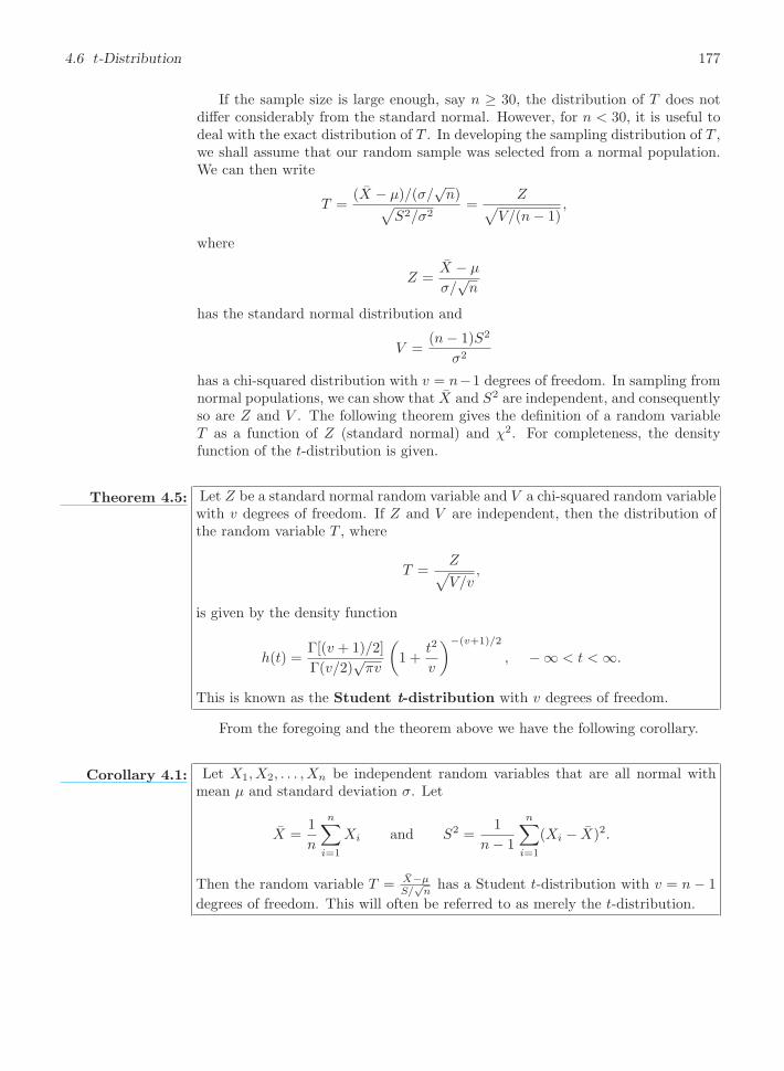
4.6 t-Distribution 177
If the sample size is large enough, say n ≥ 30, the distribution of T does notdiffer considerably from the standard normal. However, for n < 30, it is useful todeal with the exact distribution of T . In developing the sampling distribution of T ,we shall assume that our random sample was selected from a normal population.We can then write
T =(X − μ)/(σ/
√n)√
S2/σ2=
Z√V/(n− 1)
,
where
Z =X − μ
σ/√n
has the standard normal distribution and
V =(n− 1)S2
σ2
has a chi-squared distribution with v = n−1 degrees of freedom. In sampling fromnormal populations, we can show that X and S2 are independent, and consequentlyso are Z and V . The following theorem gives the definition of a random variableT as a function of Z (standard normal) and χ2. For completeness, the densityfunction of the t-distribution is given.
Theorem 4.5: Let Z be a standard normal random variable and V a chi-squared random variablewith v degrees of freedom. If Z and V are independent, then the distribution ofthe random variable T , where
T =Z√V/v
,
is given by the density function
h(t) =Γ[(v + 1)/2]
Γ(v/2)√πv
(1 +
t2
v
)−(v+1)/2
, −∞ < t < ∞.
This is known as the Student t-distribution with v degrees of freedom.
From the foregoing and the theorem above we have the following corollary.
Corollary 4.1: Let X1, X2, . . . , Xn be independent random variables that are all normal withmean μ and standard deviation σ. Let
X =1
n
n∑i=1
Xi and S2 =1
n− 1
n∑i=1
(Xi − X)2.
Then the random variable T = X−μS/
√nhas a Student t-distribution with v = n− 1
degrees of freedom. This will often be referred to as merely the t-distribution.

178 Chapter 4 Sampling Distributions and Data Descriptions
What Does the t-Distribution Look Like?
The distribution of T is similar to the distribution of Z in that they both aresymmetric about a mean of zero. Both distributions are bell shaped, but the t-distribution is more variable, owing to the fact that the T -values depend on thefluctuations of two quantities, X and S2, whereas the Z-values depend only on thechanges in X from sample to sample. The distribution of T differs from that of Zin that the variance of T depends on the sample size n and is always greater than1. Only when the sample size n → ∞ will the two distributions become the same.In Figure 4.7, we show the relationship between a standard normal distribution(v = ∞) and t-distributions with 2 and 5 degrees of freedom. The percentagepoints of the t-distribution are given in Table A.4.
�2 �1 0 1 2
v � 2
v � �
v � 5
Figure 4.7: The t-distribution curves for v = 2, 5,and ∞.
tt1� � �t t0
ααα
Figure 4.8: Symmetry property (about 0) of thet-distribution.
It is customary to let tα represent the t-value above which we find an area equalto α. Hence, the t-value with 10 degrees of freedom leaving an area of 0.025 tothe right is t = 2.228. Since the t-distribution is symmetric about a mean of zero,we have t1−α = −tα; that is, the t-value leaving an area of 1− α to the right andtherefore an area of α to the left is equal to the negative t-value that leaves an areaof α in the right tail of the distribution (see Figure 4.8). That is, t0.95 = −t0.05,t0.99 = −t0.01, and so forth.
Example 4.7: The t-value with v = 14 degrees of freedom that leaves an area of 0.025 to theleft, and therefore an area of 0.975 to the right, is
t0.975 = −t0.025 = −2.145.
Example 4.8: Find P (−t0.025 < T < t0.05).Solution : Since t0.05 leaves an area of 0.05 to the right, and −t0.025 leaves an area of 0.025
to the left, we find a total area of
1− 0.05− 0.025 = 0.925
between −t0.025 and t0.05. Hence
P (−t0.025 < T < t0.05) = 0.925.

4.6 t-Distribution 179
Example 4.9: Find k such that P (k < T < −1.761) = 0.045 for a random sample of size 15
selected from a normal distribution and T = X−μs/
√n.
t0k − t0.005
0.045
Figure 4.9: The t-values for Example 4.9.
Solution : From Table A.4 we note that 1.761 corresponds to t0.05 when v = 14. Therefore,−t0.05 = −1.761. Since k in the original probability statement is to the left of−t0.05 = −1.761, let k = −tα. Then, from Figure 4.9, we have
0.045 = 0.05− α, or α = 0.005.
Hence, from Table A.4 with v = 14,
k = −t0.005 = −2.977 and P (−2.977 < T < −1.761) = 0.045.
Example 4.10: A chemical engineer claims that the population mean yield of a certain batchprocess is 500 grams per liter of raw material. To check this claim he samples 25batches each month. If the computed t-value falls between −t0.05 and t0.05, he issatisfied with this claim. What conclusion should he draw from a sample that hasa mean x = 518 grams per liter and a sample standard deviation s = 40 grams?Assume the distribution of yields to be approximately normal.
Solution : From Table A.4 we find that t0.05 = 1.711 for 24 degrees of freedom. Therefore, theengineer can be satisfied with his claim if a sample of 25 batches yields a t-valuebetween −1.711 and 1.711. If μ = 500, then
t =518− 500
40/√25
= 2.25,
a value well above 1.711. The probability of obtaining a t-value, with v = 24, equalto or greater than 2.25 is approximately 0.02. If μ > 500, the value of t computedfrom the sample is more reasonable. Hence, the engineer is likely to conclude thatthe process produces a better product than he thought.
What Is the t-Distribution Used For?
The t-distribution is used extensively in problems that deal with inference aboutthe population mean (as illustrated in Example 4.10) or in problems that involve

180 Chapter 4 Sampling Distributions and Data Descriptions
comparative samples (i.e., in cases where one is trying to determine if means fromtwo samples are significantly different). The use of the distribution will be extendedin Chapters 5, 6, and 7. The reader should note that use of the t-distribution forthe statistic
T =X − μ
S/√n
requires that X1, X2, . . . , Xn be normal. The use of the t-distribution and thesample size consideration do not relate to the Central Limit Theorem. The useof the standard normal distribution rather than T for n ≥ 30 merely implies thatS is a sufficiently good estimator of σ in this case. In chapters that follow thet-distribution finds extensive usage.
4.7 F -Distribution
We have motivated the t-distribution in part by its application to problems in whichthere is comparative sampling (i.e., a comparison between two sample means). Forexample, some of our examples in future chapters will take a more formal approach:a chemical engineer collects data on two catalysts, a biologist collects data ontwo growth media, or a chemist gathers data on two methods of coating materialto inhibit corrosion. While it is of interest to let sample information shed lighton two population means, it is often the case that a comparison of variability isequally important, if not more so. The F -distribution finds enormous applicationin comparing sample variances. Applications of the F -distribution are found inproblems involving two or more samples.
The statistic F is defined to be the ratio of two independent chi-squared randomvariables, each divided by its number of degrees of freedom. Hence, we can write
F =U/v1V/v2
,
where U and V are independent random variables having chi-squared distributionswith v1 and v2 degrees of freedom, respectively. We shall now state the samplingdistribution of F .
Theorem 4.6: Let U and V be two independent random variables having chi-squared distribu-tions with v1 and v2 degrees of freedom, respectively. Then the distribution of the
random variable F = U/v1
V/v2is given by the density function
h(f) =
{Γ[(v1+v2)/2](v1/v2)
v1/2
Γ(v1/2)Γ(v2/2)f(v1/2)−1
(1+v1f/v2)(v1+v2)/2 , f > 0,
0, f ≤ 0.
This is known as the F-distribution with v1 and v2 degrees of freedom (d.f.).
We will make considerable use of the random variable F in future chapters. How-ever, the density function will not be used and is given only for completeness;

4.7 F -Distribution 181
instead, we will take F values from Table A.6 in the Appendix. The curve of theF -distribution depends not only on the two parameters v1 and v2 but also on theorder in which we state them. Once these two values are given, we can identify thecurve. Typical F -distributions are shown in Figure 4.10.
f0
d.f. � (6, 10)
d.f. � (10, 30)
Figure 4.10: Typical F -distributions.
f0 f
α
α
Figure 4.11: Illustration of the fα for the F -distribution.
Let fα be the f -value above which we find an area equal to α. This is illustratedby the shaded region in Figure 4.11. Table A.6 gives values of fα only for α = 0.05and α = 0.01 for various combinations of the degrees of freedom v1 and v2. Hence,the f -value with 6 and 10 degrees of freedom, leaving an area of 0.05 to the right,is f0.05 = 3.22. By means of the following theorem, Table A.6 can also be used tofind values of f0.95 and f0.99. The proof is left for the reader.
Theorem 4.7: Writing fα(v1, v2) for fα with v1 and v2 degrees of freedom, we obtain
f1−α(v1, v2) =1
fα(v2, v1).
Thus, the f -value with 6 and 10 degrees of freedom, leaving an area of 0.95 to theright, is
f0.95(6, 10) =1
f0.05(10, 6)=
1
4.06= 0.246.
The F -Distribution with Two Sample Variances
Suppose that random samples of size n1 and n2 are selected from two normalpopulations with variances σ2
1 and σ22 , respectively. From Theorem 4.4, we know
that
χ21 =
(n1 − 1)S21
σ21
and χ22 =
(n2 − 1)S22
σ22
are random variables having chi-squared distributions with v1 = n1 − 1 and v2 =n2 − 1 degrees of freedom. Furthermore, since the samples are selected at random,

182 Chapter 4 Sampling Distributions and Data Descriptions
we are dealing with independent random variables. Then, using Theorem 4.6 withχ21 = U and χ2
2 = V , we obtain the following result.
Theorem 4.8: If S21 and S2
2 are the variances of independent random samples of size n1 and n2
taken from normal populations with variances σ21 and σ2
2 , respectively, then
F =S21/σ
21
S22/σ
22
=σ22S
21
σ21S
22
has an F -distribution with v1 = n1 − 1 and v2 = n2 − 1 degrees of freedom.
Example 4.11: A statistics department at one university gives qualifying exams for its graduatestudents. The qualifying exams consist of two parts: theory and applications. Thefollowing data summary is for student scores on these two exams in one year.
Exam n x sTheoryApplication
1616
76.288.3
13.67.5
Assuming normality on both samples, is it reasonable to believe that variancesfor the scores of both subjects are equal?
Solution : Suppose both variances, denoted respectively by σ21 and σ2
2 , are the same. UsingTheorem 4.8, we conclude that
F =S21/σ
21
S22/σ
22
=S21
S22
follows an F -distribution with degrees of freedom 15 and 15. Based on the data,we compute
f =13.62
7.52= 3.288.
From Table A.6, we find out that f0.05;15,15 = 2.33, which means that the prob-ability of S2
1/S22 being larger than 2.33 is only 5%. Since our observed f -value is
3.288, which is larger than 2.33, it would not be reasonable to assume that thevariances for the scores of both subjects are equal.
What Is the F -Distribution Used For?
We answered this question, in part, at the beginning of this section. The F -distribution is used in two-sample situations to draw inferences about the pop-ulation variances. This involves the application of Theorem 4.8. However, theF -distribution can also be applied to many other types of problems involving sam-ple variances. In fact, the F -distribution is called the variance ratio distribution.As an illustration, consider Case Study 4.2, in which two paints, A and B, werecompared with regard to mean drying time. The normal distribution applies nicely(assuming that σA and σB are known). However, suppose that there are three typesof paints to compare, say A, B, and C. We wish to determine if the population

4.8 Graphical Presentation 183
means are equivalent. Suppose that important summary information from theexperiment is as follows:
Paint Sample Mean Sample Variance Sample Size
A XA = 4.5 s2A = 0.20 10
B XB = 5.5 s2B = 0.14 10
C XC = 6.5 s2C = 0.11 10
The problem centers around whether or not the sample averages (xA, xB , xC)are far enough apart. The implication of “far enough apart” is very important.It would seem reasonable that if the variability between sample averages is largerthan what one would expect by chance, the data do not support the conclusion thatμA = μB = μC . Whether these sample averages could have occurred by chancedepends on the variability within samples, as quantified by s2A, s
2B , and s2C .
An analysis that involves all of the data would attempt to determine if thevariability between the sample averages and the variability within the samplescould have occurred jointly if in fact the populations have a common mean. Noticethat the key to this analysis centers around the two following sources of variability:
(1) Variability within samples (between observations in distinct samples)
(2) Variability between samples (between sample averages)
Clearly, if the variability in (1) is considerably larger than that in (2), there willbe considerable overlap in the sample data, a signal that the data could all havecome from a common distribution.
4.8 Graphical Presentation
Often the end result of a statistical analysis is the estimation of parameters of apostulated model. This is natural for scientists and engineers since they oftendeal in modeling. A statistical model is not deterministic but, rather, must entailsome probabilistic aspects. A model form is often the foundation of assumptionsthat are made by the analyst. For example, the scientist in Example 1.2 may wishto draw some level of distinction between the nitrogen and no-nitrogen populationsthrough the sample information. The analysis may require a certain model forthe data, for example, that the two samples come from normal or Gaussiandistributions. See Chapter 3 for a discussion of the normal distribution.
Obviously, the user of statistical methods cannot generate sufficient informationor experimental data to characterize the population totally. But sets of data areoften used to learn about certain properties of the population. Scientists and engi-neers are accustomed to dealing with data sets. The importance of characterizingor summarizing the nature of collections of data should be obvious. Often a sum-mary of a collection of data via a graphical display can provide insight regardingthe system from which the data were taken.
In this section, the role of sampling and the display of data for enhancement ofstatistical inference is explored in detail. We introduce some simple but ofteneffective displays that complement the study of statistical populations.

184 Chapter 4 Sampling Distributions and Data Descriptions
Scatter Plot
At times the model postulated may take on a somewhat complicated form. Con-sider, for example, a textile manufacturer who designs an experiment where clothspecimens that contain various percentages of cotton are produced. Consider thedata in Table 4.1.
Table 4.1: Tensile Strength
Cotton Percentage Tensile Strength
15 7, 7, 9, 8, 1020 19, 20, 21, 20, 2225 21, 21, 17, 19, 2030 8, 7, 8, 9, 10
Five cloth specimens are manufactured for each of the four cotton percentages.In this case, both the model for the experiment and the type of analysis usedshould take into account the goal of the experiment and important input fromthe textile scientist. Some simple graphics can shed important light on the cleardistinction between the samples. See Figure 4.12; the sample means and variabilityare depicted nicely in the scatter plot.
5
10
15
20
25
15 20 25 30
Ten
sile
Str
engt
h
Cotton Percentages
Figure 4.12: Scatter plot of tensile strength and cotton percentages.
One possible goal of this experiment is simply to determine which cotton per-centages are truly distinct from the others. In other words, as in the case of thenitrogen/no-nitrogen data, for which cotton percentages are there clear distinctionsbetween the populations or, more specifically, between the population means? Inthis case, perhaps a reasonable model is that each sample comes from a normaldistribution. Here the goal is very much like that of the nitrogen/no-nitrogen dataexcept that more samples are involved. The formalism of the analysis involvesnotions of hypothesis testing discussed in Chapter 6. Incidentally, this formalityis perhaps not necessary in light of the diagnostic plot. But does this describethe real goal of the experiment and hence the proper approach to data analysis?

4.8 Graphical Presentation 185
It is likely that the scientist anticipates the existence of a maximum populationmean tensile strength in the range of cotton concentration in the experiment. Herethe analysis of the data should revolve around a different type of model, one thatpostulates a type of structure relating the population mean tensile strength to thecotton concentration. In other words, a model may be written
μt,c = β0 + β1C + β2C2,
where μt,c is the population mean tensile strength, which varies with the amountof cotton in the product C. The implication of this model is that for a fixed cottonlevel, there is a population of tensile strength measurements and the populationmean is μt,c. This type of model, called a regression model, is discussed in Chap-ter 7. The functional form is chosen by the scientist. At times the data analysismay suggest that the model be changed. Then the data analyst “entertains” amodel that may be altered after some analysis is done. The use of an empiricalmodel is accompanied by estimation theory, where β0, β1, and β2 are estimatedby the data. Further, statistical inference can then be used to determine modeladequacy.
Two points become evident from the two data illustrations here: (1) The typeof model used to describe the data often depends on the goal of the experiment;and (2) the structure of the model should take advantage of nonstatistical scientificinput. A selection of a model represents a fundamental assumption upon whichthe resulting statistical inference is based.
It will become apparent throughout the book how important graphics can be.Often, plots can illustrate information that allows the results of the formal statisti-cal inference to be better communicated to the scientist or engineer. At times, plotsor exploratory data analysis can teach the analyst something not retrieved fromthe formal analysis. Almost any formal analysis requires assumptions that evolvefrom the model of the data. Graphics can nicely highlight violation of assump-tions that would otherwise go unnoticed. Throughout the book, graphics are usedextensively to supplement formal data analysis. The following sections reveal somegraphical tools that are useful in exploratory or descriptive data analysis.
Stem-and-Leaf Plot
Statistical data, generated in large masses, can be very useful for studying thebehavior of the distribution if presented in a combined tabular and graphic displaycalled a stem-and-leaf plot.
To illustrate the construction of a stem-and-leaf plot, consider the data of Table4.2, which specifies the “life” of 40 similar car batteries recorded to the nearest tenthof a year. The batteries are guaranteed to last 3 years. First, split each observationinto two parts consisting of a stem and a leaf such that the stem represents thedigit preceding the decimal and the leaf corresponds to the decimal part of thenumber. In other words, for the number 3.7, the digit 3 is designated the stem andthe digit 7 is the leaf. The four stems 1, 2, 3, and 4 for our data are listed verticallyon the left side in Table 4.3; the leaves are recorded on the right side opposite theappropriate stem value. Thus, the leaf 6 of the number 1.6 is recorded oppositethe stem 1; the leaf 5 of the number 2.5 is recorded opposite the stem 2; and so

186 Chapter 4 Sampling Distributions and Data Descriptions
forth. The number of leaves recorded opposite each stem is summarized under thefrequency column.
Table 4.2: Car Battery Life
2.2 4.1 3.5 4.5 3.2 3.7 3.0 2.63.4 1.6 3.1 3.3 3.8 3.1 4.7 3.72.5 4.3 3.4 3.6 2.9 3.3 3.9 3.13.3 3.1 3.7 4.4 3.2 4.1 1.9 3.44.7 3.8 3.2 2.6 3.9 3.0 4.2 3.5
Table 4.3: Stem-and-Leaf Plot of Battery Life
Stem Leaf Frequency1234
6925669001111222333444556777889911234577
25258
The stem-and-leaf plot of Table 4.3 contains only four stems and consequentlydoes not provide an adequate picture of the distribution. To remedy this problem,we need to increase the number of stems in our plot. One simple way to accomplishthis is to write each stem value twice and then record the leaves 0, 1, 2, 3, and 4opposite the appropriate stem value where it appears for the first time, and theleaves 5, 6, 7, 8, and 9 opposite this same stem value where it appears for the secondtime. This modified double-stem-and-leaf plot is illustrated in Table 4.4, where thestems corresponding to leaves 0 through 4 have been coded by the symbol � andthe stems corresponding to leaves 5 through 9 by the symbol ·.
Table 4.4: Double-Stem-and-Leaf Plot of Battery Life
Stem Leaf Frequency1·2�2·3�3·4�4·
6925669001111222333444556777889911234577
214
151053
In any given problem, we must decide on the appropriate stem values. Thisdecision is made somewhat arbitrarily, although we are guided by the size of oursample. Usually, we choose between 5 and 20 stems. The smaller the number ofdata available, the smaller is our choice for the number of stems. For example, ifthe data consist of numbers from 1 to 21 representing the number of people in acafeteria line on 40 randomly selected workdays and we choose a double-stem-and-leaf plot, the stems will be 0�, 0·, 1�, 1·, and 2� so that the smallest observation

4.8 Graphical Presentation 187
1 has stem 0� and leaf 1, the number 18 has stem 1· and leaf 8, and the largestobservation 21 has stem 2� and leaf 1. On the other hand, if the data consist ofnumbers from $18,800 to $19,600 representing the best possible deals on 100 newautomobiles from a certain dealership and we choose a single-stem-and-leaf plot,the stems will be 188, 189, 190, . . . , 196 and the leaves will now each contain twodigits. A car that sold for $19,385 would have a stem value of 193 and the two-digitleaf 85. Multiple-digit leaves belonging to the same stem are usually separated bycommas in the stem-and-leaf plot. Decimal points in the data are generally ignoredwhen all the digits to the right of the decimal represent the leaf. Such was thecase in Tables 4.3 and 4.4. However, if the data consist of numbers ranging from21.8 to 74.9, we might choose the digits 2, 3, 4, 5, 6, and 7 as our stems so that anumber such as 48.3 would have a stem value of 4 and a leaf of 8.3.
The stem-and-leaf plot represents an effective way to summarize data. Anotherway is through the use of the frequency distribution, where the data, groupedinto different classes or intervals, can be constructed by counting the leaves be-longing to each stem and noting that each stem defines a class interval. In Table4.3, the stem 1 with 2 leaves defines the interval 1.0–1.9 containing 2 observations;the stem 2 with 5 leaves defines the interval 2.0–2.9 containing 5 observations; thestem 3 with 25 leaves defines the interval 3.0–3.9 with 25 observations; and thestem 4 with 8 leaves defines the interval 4.0–4.9 containing 8 observations. For thedouble-stem-and-leaf plot of Table 4.4, the stems define the seven class intervals1.5–1.9, 2.0–2.4, 2.5–2.9, 3.0–3.4, 3.5–3.9, 4.0–4.4, and 4.5–4.9 with frequencies 2,1, 4, 15, 10, 5, and 3, respectively.
Histogram
Dividing each class frequency by the total number of observations, we obtain theproportion of the set of observations in each of the classes. A table listing relativefrequencies is called a relative frequency distribution. The relative frequencydistribution for the data of Table 4.2, showing the midpoint of each class interval,is given in Table 4.5.
Table 4.5: Relative Frequency Distribution of Battery Life
Class Class Frequency, RelativeInterval Midpoint f Frequency1.5–1.9 1.7 2 0.0502.0–2.4 2.2 1 0.0252.5–2.9 2.7 4 0.1003.0–3.4 3.2 15 0.3753.5–3.9 3.7 10 0.2504.0–4.4 4.2 5 0.1254.5–4.9 4.7 3 0.075
The information provided by a relative frequency distribution in tabular form iseasier to grasp if presented graphically. Using the midpoint of each interval and thecorresponding relative frequency, we construct a relative frequency histogram(Figure 4.13).

188 Chapter 4 Sampling Distributions and Data Descriptions
0.375
0.250
0.125
1.7 2.2 2.7 3.2 3.7 4.2 4.7
Rel
ativ
e F
requ
enct
y
Battery Life (years)
Figure 4.13: Relative frequency histogram.
Many continuous frequency distributions can be represented graphically by thecharacteristic bell-shaped curve of Figure 4.14. Graphical tools such as what we seein Figures 4.13 and 4.14 aid in the characterization of the nature of the population.
0
f (x )
Battery Life (years)1 2 3 4 5 6
Figure 4.14: Estimating frequency distribution.
A distribution is said to be symmetric if it can be folded along a vertical axisso that the two sides coincide. A distribution that lacks symmetry with respect toa vertical axis is said to be skewed. The distribution illustrated in Figure 4.15(a)is said to be skewed to the right since it has a long right tail and a much shorter lefttail. In Figure 4.15(b) we see that the distribution is symmetric, while in Figure4.15(c) it is skewed to the left.
If we rotate a stem-and-leaf plot counterclockwise through an angle of 90◦,we observe that the resulting columns of leaves form a picture that is similarto a histogram. Consequently, if our primary purpose in looking at the data is todetermine the general shape or form of the distribution, it will seldom be necessaryto construct a relative frequency histogram.

4.8 Graphical Presentation 189
(a) (b) (c)
Figure 4.15: Skewness of data.
Box-and-Whisker Plot or Box Plot
Another display that is helpful for reflecting properties of a sample is the box-and-whisker plot. This plot encloses the interquartile range of the data in a boxthat has the median displayed within. The interquartile range has as its extremesthe 75th percentile (upper quartile) and the 25th percentile (lower quartile). Inaddition to the box, “whiskers” extend, showing extreme observations in the sam-ple. For reasonably large samples, the display shows center of location, variability,and the degree of asymmetry.
In addition, a variation called a box plot can provide the viewer with infor-mation regarding which observations may be outliers. Outliers are observationsthat are considered to be unusually far from the bulk of the data. There are manystatistical tests that are designed to detect outliers. Technically, one may viewan outlier as being an observation that represents a “rare event” (there is a smallprobability of obtaining a value that far from the bulk of the data). The conceptof outliers resurfaces in Chapter 7 in the context of regression analysis.
The visual information in the box-and-whisker plot or box plot is not intendedto be a formal test for outliers. Rather, it is viewed as a diagnostic tool. While thedetermination of which observations are outliers varies with the type of softwarethat is used, one common procedure is to use a multiple of the interquartilerange. For example, if its distance from the box exceeds 1.5 times the interquartilerange (in either direction), an observation may be labeled an outlier.
Example 4.12: Nicotine content was measured in a random sample of 40 cigarettes. The data aredisplayed in Table 4.6.
Table 4.6: Nicotine Data for Example 4.12
1.09 1.92 2.31 1.79 2.28 1.74 1.47 1.970.85 1.24 1.58 2.03 1.70 2.17 2.55 2.111.86 1.90 1.68 1.51 1.64 0.72 1.69 1.851.82 1.79 2.46 1.88 2.08 1.67 1.37 1.931.40 1.64 2.09 1.75 1.63 2.37 1.75 1.69

190 Chapter 4 Sampling Distributions and Data Descriptions
1.0 1.5 2.0 2.5
Nicotine
Figure 4.16: Box-and-whisker plot for Example 4.12.
The decimal point is 1 digit(s) to the left of the |
7 | 2
8 | 5
9 |
10 | 9
11 |
12 | 4
13 | 7
14 | 07
15 | 18
16 | 3447899
17 | 045599
18 | 2568
19 | 0237
20 | 389
21 | 17
22 | 8
23 | 17
24 | 6
25 | 5
Figure 4.17: Stem-and-leaf plot for the nicotine data.
Figure 4.16 shows the box-and-whisker plot of the data, depicting the obser-vations 0.72 and 0.85 as mild outliers in the lower tail, whereas the observation2.55 is a mild outlier in the upper tail. In this example, the interquartile rangeis 0.365, and 1.5 times the interquartile range is 0.5475. Figure 4.17 provides astem-and-leaf plot of the data.
Exercises
4.28 For a chi-squared distribution, find
(a) χ20.005 when v = 5;
(b) χ20.05 when v = 19;
(c) χ20.01 when v = 12.
4.29 For a chi-squared distribution, find

Exercises 191
(a) χ20.025 when v = 15;
(b) χ20.01 when v = 7;
(c) χ20.05 when v = 24.
4.30 For a chi-squared distribution, find χ2α such that
(a) P (X2 > χ2α) = 0.01 when v = 21;
(b) P (X2 < χ2α) = 0.95 when v = 6;
(c) P (χ2α < X2 < 23.209) = 0.015 when v = 10.
4.31 For a chi-squared distribution, find χ2α such that
(a) P (X2 > χ2α) = 0.99 when v = 4;
(b) P (X2 > χ2α) = 0.025 when v = 19;
(c) P (37.652 < X2 < χ2α) = 0.045 when v = 25.
4.32 The scores on a placement test given to collegefreshmen for the past five years are approximately nor-mally distributed with a mean μ = 74 and a varianceσ2 = 8. Would you still consider σ2 = 8 to be a validvalue of the variance if a random sample of 20 studentswho take the placement test this year obtain a value ofs2 = 20?
4.33 Assume the sample variances to be continuousmeasurements. Find the probability that a randomsample of 25 observations, from a normal populationwith variance σ2 = 6, will have a sample variance S2
(a) greater than 9.1;
(b) between 3.462 and 10.745.
4.34 Show that the variance of S2 for random sam-ples of size n from a normal population decreases asn becomes large. [Hint: First find the variance of(n− 1)S2/σ2.]
4.35 (a) Find P (T < 2.365) when v = 7.
(b) Find P (T > 1.318) when v = 24.
(c) Find P (−1.356 < T < 2.179) when v = 12.
(d) Find P (T > −2.567) when v = 17.
4.36 (a) Find t0.025 when v = 14.
(b) Find −t0.10 when v = 10.
(c) Find t0.995 when v = 7.
4.37 Given a random sample of size 24 from a normaldistribution, find k such that
(a) P (−2.069 < T < k) = 0.965;
(b) P (k < T < 2.807) = 0.095;
(c) P (−k < T < k) = 0.90.
4.38 (a) Find P (−t0.005 < T < t0.01) for v = 20.
(b) Find P (T > −t0.025).
4.39 A manufacturing firm claims that the batter-ies used in its electronic games will last an average of30 hours. To maintain this average, 16 batteries aretested each month. If the computed t-value falls be-tween −t0.025 and t0.025, the firm is satisfied with itsclaim. What conclusion should the firm draw from asample that has a mean of x = 27.5 hours and a stan-dard deviation of s = 5 hours? Assume the distributionof battery lives to be approximately normal.
4.40 A maker of a certain brand of low-fat cereal barsclaims that the average saturated fat content is 0.5gram. In a random sample of 8 cereal bars of thisbrand, the saturated fat content was 0.6, 0.7, 0.7, 0.3,0.4, 0.5, 0.4, and 0.2. Would you agree with the claim?Assume a normal distribution.
4.41 For an F -distribution, find
(a) f0.05 with v1 = 7 and v2 = 15;
(b) f0.05 with v1 = 15 and v2 = 7:
(c) f0.01 with v1 = 24 and v2 = 19;
(d) f0.95 with v1 = 19 and v2 = 24;
(e) f0.99 with v1 = 28 and v2 = 12.
4.42 Construct a box-and-whisker plot of these data,which represent the lifetimes, in hours, of fifty 40-watt,110-volt internally frosted incandescent lamps takenfrom forced life tests:
919 1196 785 1126 936 9181156 920 948 1067 1092 11621170 929 950 905 972 10351045 855 1195 1195 1340 1122938 970 1237 956 1102 1157978 832 1009 1157 1151 1009765 958 902 1022 1333 811
1217 1085 896 958 1311 1037702 923
4.43 Consider the following measurements of theheat-producing capacity of the coal produced by twomines (in millions of calories per ton):
Mine 1: 8260 8130 8350 8070 8340Mine 2: 7950 7890 7900 8140 7920 7840
Can it be concluded that the two population variancesare equal?
4.44 Pull-strength tests on 10 soldered leads for asemiconductor device yield the following results, inpounds of force required to rupture the bond:
19.8 12.7 13.2 16.9 10.618.8 11.1 14.3 17.0 12.5
Another set of 8 leads was tested after encapsulationto determine whether the pull strength had been in-

192 Chapter 4 Sampling Distributions and Data Descriptions
creased by encapsulation of the device, with the fol-lowing results:
24.9 22.8 23.6 22.1 20.4 21.6 21.8 22.5
Comment on the evidence available concerning equal-ity of the two population variances.
Review Exercises
4.45 The following data represent the length of life,in seconds, of 50 fruit flies subject to a new spray in acontrolled laboratory experiment:
17 20 10 9 23 13 12 19 18 2412 14 6 9 13 6 7 10 13 716 18 8 13 3 32 9 7 10 1113 7 18 7 10 4 27 19 16 87 10 5 14 15 10 9 6 7 15
Construct a box-and-whisker plot and comment on thenature of the sample. Compute the sample mean andsample standard deviation.
4.46 In testing for carbon monoxide in a certainbrand of cigarette, the data, in milligrams percigarette, were coded by subtracting 12 from each ob-servation. Use the results of Exercise 4.10 on page 163to find the sample standard deviation for the carbonmonoxide content of a random sample of 15 cigarettesof this brand if the coded measurements are 3.8, −0.9,5.4, 4.5, 5.2, 5.6, 2.7, −0.1, −0.3, −1.7, 5.7, 3.3, 4.4,−0.5, and 1.9.
4.47 If S21 and S2
2 represent the variances of indepen-dent random samples of size n1 = 8 and n2 = 12,taken from normal populations with equal variances,find P (S2
1/S22 < 4.89).
4.48 If the number of hurricanes that hit a certainarea of the eastern United States per year is a randomvariable having a Poisson distribution with μ = 6, findthe probability that this area will be hit by
(a) exactly 15 hurricanes in 2 years;
(b) at most 9 hurricanes in 2 years.
4.49 The following data represent the length of life inyears, measured to the nearest tenth, of 30 similar fuelpumps:
2.0 3.0 0.3 3.3 1.3 0.40.2 6.0 5.5 6.5 0.2 2.31.5 4.0 5.9 1.8 4.7 0.74.5 0.3 1.5 0.5 2.5 5.01.0 6.0 5.6 6.0 1.2 0.2
Construct a box-and-whisker plot. Comment on theoutliers in the data.
4.50 If S21 and S2
2 represent the variances of indepen-dent random samples of size n1 = 25 and n2 = 31,taken from normal populations with variances σ2
1 = 10
and σ22 = 15, respectively, find
P (S21/S
22 > 1.26).
4.51 Consider Example 4.12 on page 189. Commenton any outliers.
4.52 The breaking strength X of a certain rivet usedin a machine engine has a mean 5000 psi and stan-dard deviation 400 psi. A random sample of 36 rivetsis taken. Consider the distribution of X, the samplemean breaking strength.
(a) What is the probability that the sample mean fallsbetween 4800 psi and 5200 psi?
(b) What sample n would be necessary in order to have
P (4900 < X < 5100) = 0.99?
4.53 A taxi company tests a random sample of 10steel-belted radial tires of a certain brand and recordsthe following tread wear: 48,000, 53,000, 45,000,61,000, 59,000, 56,000, 63,000, 49,000, 53,000, and54,000 kilometers. The marketing claim for the tiresis that, on the average, the tires last for 53,000 kilome-ters of use. In your answer, compute
t =x− 53, 000
s/√10
and determine from Table A.4 (with 9 degrees of free-dom) whether the computed t-value is reasonable orappears to be a rare event.
4.54 Two distinct solid fuel propellants, type A andtype B, are being considered for a space program activ-ity. Burning rates of the propellant are crucial. Ran-dom samples of 20 specimens of the two propellantsare taken with sample means 20.5 cm/sec for propel-lant A and 24.50 cm/sec for propellant B. It is gen-erally assumed that the variability in burning rate isroughly the same for the two propellants and is givenby a population standard deviation of 5 cm/sec. As-sume that the burning rates for the propellants areapproximately normal and hence make use of the Cen-tral Limit Theorem. Nothing is known about the twopopulation mean burning rates, and it is hoped thatthis experiment might shed some light on them.
(a) If, indeed, μA = μB , what is P (XB − XA ≥ 4.0)?

Review Exercises 193
(b) Use your answer in (a) to shed some light on theproposition that μA = μB .
4.55 The concentration of an active ingredient in theoutput of a chemical reaction is strongly influenced bythe catalyst that is used in the reaction. It is believedthat when catalyst A is used, the population meanconcentration exceeds 65%. The standard deviationis known to be σ = 5%. A sample of outputs from 30independent experiments gives the average concentra-tion of xA = 64.5%.
(a) Does this sample information with an average con-centration of xA = 64.5% provide disturbing in-formation that perhaps μA is not 65%, but lessthan 65%? Support your answer with a probabilitystatement.
(b) Suppose a similar experiment is done with the useof another catalyst, catalyst B. The standard devi-ation σ is still assumed to be 5% and xB turns outto be 70%. Comment on whether or not the sampleinformation on catalyst B strongly suggests thatμB is truly greater than μA. Support your answerby computing
P (XB − XA ≥ 5.5 | μB = μA).
(c) Under the condition that μA = μB = 65%, give theapproximate distribution of the following quantities(with mean and variance of each). Make use of theCentral Limit Theorem.
i)XB ;ii)XA − XB ;
iii) XA−XB
σ√
2/30.
4.56 From the information in Review Exercise 4.55,compute (assuming μB = 65%) P (XB ≥ 70).
4.57 Given a normal random variable X with mean20 and variance 9, and a random sample of size n takenfrom the distribution, what sample size n is necessaryin order that
P (19.9 ≤ X ≤ 20.1) = 0.95?
4.58 In Chapter 5, the concept of parameter esti-mation will be discussed at length. Suppose X is arandom variable with mean μ and variance σ2 = 1.0.Suppose also that a random sample of size n is to betaken and x is to be used as an estimate of μ. Whenthe data are taken and the sample mean is measured,we wish it to be within 0.05 unit of the true mean with
probability 0.99. That is, we want there to be a goodchance that the computed x from the sample is “veryclose” to the population mean (wherever it is!), so wewish
P (|X − μ| > 0.05) = 0.99.
What sample size is required?
4.59 Suppose a filling machine is used to fill cartonswith a liquid product. The specification that is strictlyenforced for the filling machine is 9 ± 1.5 oz. If any car-ton is produced with weight outside these bounds, it isconsidered by the supplier to be defective. It is hopedthat at least 99% of cartons will meet these specifica-tions. With the conditions μ = 9 and σ = 1, whatproportion of cartons from the process are defective?If changes are made to reduce variability, what mustσ be reduced to in order to meet specifications withprobability 0.99? Assume a normal distribution forthe weight.
4.60 Consider the situation in Review Exercise 4.59.Suppose a considerable effort is conducted to “tighten”the variability in the system. Following the effort, arandom sample of size 40 is taken from the new assem-bly line and the sample variance is s2 = 0.188 ounces2.Do we have strong numerical evidence that σ2 has beenreduced below 1.0? Consider the probability
P (S2 ≤ 0.188 | σ2 = 1.0),
and give your conclusion.
4.61 Group Project: The class should be dividedinto groups of four people. The four students in eachgroup should go to the college gym or a local fit-ness center. The students should ask each person whocomes through the door his or her height in inches.Each group will then divide the height data by genderand work together to answer the following questions.
(a) Construct a histogram for each gender of the data.Based on these plots, do the data appear to followa normal distribution?
(b) Use the estimated sample variance as the true vari-ance for each gender. Assume that the populationmean height for male students is actually 3 inchesmore than that of female students. What is theprobability that the average height of the male stu-dents will be 4 inches more than that of the femalestudents in your sample?
(c) What factors could render these results misleading?

194 Chapter 4 Sampling Distributions and Data Descriptions
4.9 Potential Misconceptions and Hazards;Relationship to Material in Other Chapters
The Central Limit Theorem is one of the most powerful tools in all of statistics, andeven though this chapter is relatively short, it contains a wealth of fundamentalinformation about tools that will be used throughout the balance of the text.
The notion of a sampling distribution is one of the most important fundamentalconcepts in all of statistics, and the student at this point in his or her trainingshould gain a clear understanding of it before proceeding beyond this chapter. Allchapters that follow will make considerable use of sampling distributions. Supposeone wants to use the statistic X to draw inferences about the population meanμ. This will be done by using the observed value x from a single sample of sizen. Then any inference made must be accomplished by taking into account notjust the single value but rather the theoretical structure, or distribution of all xvalues that could be observed from samples of size n. Thus, the concept ofa sampling distribution comes to the surface. This distribution is the basis for theCentral Limit Theorem. The t, χ2, and F-distributions are also used in the contextof sampling distributions. For example, the t-distribution, pictured in Figure 4.7,represents the structure that occurs if all of the values of x−μ
s/√nare formed, where
x and s are taken from samples of size n from a n(x;μ, σ) distribution. Similarremarks can be made about χ2 and F , and the reader should not forget that thesample information forming the statistics for all of these distributions is the normal.So it can be said that where there is a t, F, or χ2, the source was a samplefrom a normal distribution.
The three distributions described above may appear to have been introduced ina rather self-contained fashion with no indication of what they are about. However,they will appear in practical problem-solving throughout the balance of the text.
Now, there are three things that one must bear in mind, lest confusion set inregarding these fundamental sampling distributions:
(i) One cannot use the Central Limit Theorem unless σ is known. When σ is notknown, it should be replaced by s, the sample standard deviation, in order touse the Central Limit Theorem.
(ii) The T statistic is not a result of the Central Limit Theorem and x1, x2, . . . , xn
must come from a n(x;μ, σ) distribution in order for x−μs/
√nto be a t-distribution;
s is, of course, merely an estimate of σ.
(iii) While the notion of degrees of freedom is new at this point, the conceptshould be very intuitive, since it is reasonable that the nature of the distri-bution of S and also t should depend on the amount of information in thesample x1, x2, . . . , xn.

Chapter 5
One- and Two-SampleEstimation Problems
5.1 Introduction
In previous chapters, we emphasized sampling properties of the sample mean andvariance. We also emphasized displays of data in various forms. The purpose ofthese presentations is to build a foundation that allows us to draw conclusions aboutthe population parameters from experimental data. For example, the Central LimitTheorem provides information about the distribution of the sample mean X. Thedistribution involves the population mean μ. Thus, any conclusions concerning μdrawn from an observed sample average must depend on knowledge of this samplingdistribution. Similar comments apply to S2 and σ2. Clearly, any conclusions wedraw about the variance of a normal distribution will likely involve the samplingdistribution of S2.
In this chapter, we begin by formally outlining the purpose of statistical in-ference. We follow this by discussing the problem of estimation of populationparameters. We confine our formal developments of specific estimation proce-dures to problems involving one and two samples.
5.2 Statistical Inference
In Chapter 1, we discussed the general philosophy of formal statistical inference.Statistical inference consists of those methods by which one makes inferences orgeneralizations about a population. The trend today is to distinguish between theclassical method of estimating a population parameter, whereby inferences arebased strictly on information obtained from a random sample selected from thepopulation, and the Bayesian method, which utilizes prior subjective knowledgeabout the probability distribution of the unknown parameters in conjunction withthe information provided by the sample data. Throughout most of this chapter,we shall use classical methods to estimate unknown population parameters such asthe mean, the proportion, and the variance by computing statistics from random
195

196 Chapter 5 One- and Two-Sample Estimation Problems
samples and applying the theory of sampling distributions, much of which wascovered in Chapter 4.
Statistical inference may be divided into two major areas: estimation andtests of hypotheses. We treat these two areas separately, dealing with theoryand applications of estimation in this chapter and hypothesis testing in Chapter6. To distinguish clearly between the two areas, consider the following examples.A candidate for public office may wish to estimate the true proportion of votersfavoring him by obtaining opinions from a random sample of 100 eligible voters.The fraction of voters in the sample favoring the candidate could be used as anestimate of the true proportion in the population of voters. A knowledge of thesampling distribution of a proportion enables one to establish the degree of accuracyof such an estimate. This problem falls in the area of estimation.
Now consider the case in which one is interested in finding out whether brandA floor wax is more scuff-resistant than brand B floor wax. He or she mighthypothesize that brandA is better than brandB and, after proper testing, accept orreject this hypothesis. In this example, we do not attempt to estimate a parameter,but instead we try to arrive at a correct decision about a prestated hypothesis.Once again we are dependent on sampling theory and the use of data to provideus with some measure of accuracy for our decision.
5.3 Classical Methods of Estimation
A point estimate of some population parameter θ is a single value θ of a statisticΘ. For example, the value x of the statistic X, computed from a sample of size n,is a point estimate of the population parameter μ. Similarly, p = x/n is a pointestimate of the true proportion p for a binomial experiment.
An estimator is not expected to estimate the population parameter withouterror. We do not expect X to estimate μ exactly, but we certainly hope that it isnot far off. For a particular sample, it is possible to obtain a closer estimate of μby using the sample median X as an estimator. Consider, for instance, a sampleconsisting of the values 2, 5, and 11 from a population whose mean is 4 but issupposedly unknown. We would estimate μ to be x = 6, using the sample meanas our estimate, or x = 5, using the sample median as our estimate. In this case,the estimator X produces an estimate closer to the true parameter than does theestimator X. On the other hand, if our random sample contains the values 2, 6,and 7, then x = 5 and x = 6, so X is the better estimator. Not knowing the truevalue of μ, we must decide in advance whether to use X or X as our estimator.
Unbiased Estimator
What are the desirable properties of a “good” decision function that would influ-ence us to choose one estimator rather than another? Let Θ be an estimator whosevalue θ is a point estimate of some unknown population parameter θ. Certainly, wewould like the sampling distribution of Θ to have a mean equal to the parameterestimated. An estimator possessing this property is said to be unbiased.

5.3 Classical Methods of Estimation 197
Definition 5.1: A statistic Θ is said to be an unbiased estimator of the parameter θ if
μΘ = E(Θ) = θ.
Example 5.1: If a sample X1, . . . , Xn has an unknown population mean μ, then the sample meanX is an unbiased estimator for μ.
Solution : This result can be easily shown as
E(X) = E
(1
n
n∑i=1
Xi
)=
1
n
n∑i=1
E(Xi) =1
n
n∑i=1
μ = μ.
This means that the sample mean is always unbiased to the population mean.
Example 5.2: Show that S2 is an unbiased estimator of the parameter σ2.Solution : One can show that (see Exercise 5.10)
n∑i=1
(Xi − X)2 =n∑
i=1
(Xi − μ)2 − n(X − μ)2.
Now
E(S2) = E
[1
n− 1
n∑i=1
(Xi − X)2
]
=1
n− 1
[n∑
i=1
E(Xi − μ)2 − nE(X − μ)2
]=
1
n− 1
(n∑
i=1
σ2Xi
− nσ2X
).
However,
σ2Xi
= σ2, for i = 1, 2, . . . , n, and σ2X =
σ2
n.
Therefore,
E(S2) =1
n− 1
(nσ2 − n
σ2
n
)= σ2.
This result shows that the sample variance is always unbiased to the populationvariance σ2.
Although S2 is an unbiased estimator of σ2, S, on the other hand, is usually abiased estimator of σ, with the bias becoming insignificant for large samples. Thisexample illustrates why we divide by n − 1 rather than n when the variance isestimated.
Variance of a Point Estimator
If Θ1 and Θ2 are two unbiased estimators of the same population parameter θ, wewant to choose the estimator whose sampling distribution has the smaller variance.Hence, if σ2
θ1< σ2
θ2, we say that Θ1 is a more efficient estimator of θ than Θ2.

198 Chapter 5 One- and Two-Sample Estimation Problems
Definition 5.2: If we consider all possible unbiased estimators of some parameter θ, the one withthe smallest variance is called the most efficient estimator of θ.
Figure 5.1 illustrates the sampling distributions of three different estimators,Θ1, Θ2, and Θ3, all estimating θ. It is clear that only Θ1 and Θ2 are unbiased,since their distributions are centered at θ. The estimator Θ1 has a smaller variancethan Θ2 and is therefore more efficient. Hence, our choice for an estimator of θ,among the three considered, would be Θ1.
θ
θ
�2^
�1^
�3^
Figure 5.1: Sampling distributions of different estimators of θ.
For normal populations, one can show that both X and X are unbiased estima-tors of the population mean μ, but the variance of X is smaller than the varianceof X. Thus, both estimates x and x will, on average, equal the population meanμ, but x is likely to be closer to μ for a given sample, and thus X is more efficientthan X.
Interval Estimation
Even the most efficient unbiased estimator is unlikely to estimate the populationparameter exactly. It is true that estimation accuracy increases with large samples,but there is still no reason we should expect a point estimate from a given sampleto be exactly equal to the population parameter it is supposed to estimate. Thereare many situations in which it is preferable to determine an interval within whichwe would expect to find the value of the parameter. Such an interval is called aninterval estimate.
An interval estimate of a population parameter θ is an interval of the formθL < θ < θU , where θL and θU depend on the value of the statistic Θ for aparticular sample and also on the sampling distribution of Θ. For example, arandom sample of SAT verbal scores for students in the entering freshman classmight produce an interval from 530 to 550, within which we expect to find thetrue average of all SAT verbal scores for the freshman class. The values of theendpoints, 530 and 550, will depend on the computed sample mean x and thesampling distribution of X. As the sample size increases, we know that σ2
X= σ2/n
decreases, and consequently our estimate is likely to be closer to the parameter μ,

5.4 Single Sample: Estimating the Mean 199
resulting in a shorter interval. Thus, the interval estimate indicates, by its length,the accuracy of the point estimate. An engineer will gain some insight into thepopulation proportion defective by taking a sample and computing the sampleproportion defective. But an interval estimate might be more informative.
Interpretation of Interval Estimates
Since different samples will generally yield different values of Θ and, therefore,different values for θL and θU , these endpoints of the interval are values of corre-sponding random variables ΘL and ΘU . From the sampling distribution of Θ weshall be able to determine ΘL and ΘU such that P (ΘL < θ < ΘU ) is equal to anypositive fractional value we care to specify. If, for instance, we find ΘL and ΘU
such that
P (ΘL < θ < ΘU ) = 1− α,
for 0 < α < 1, then we have a probability of 1−α of selecting a random sample thatwill produce an interval containing θ. The interval θL < θ < θU , computed fromthe selected sample, is called a 100(1 − α)% confidence interval, the fraction1 − α is called the confidence coefficient or the degree of confidence, andthe endpoints, θL and θU , are called the lower and upper confidence limits.Thus, when α = 0.05, we have a 95% confidence interval, and when α = 0.01, weobtain a wider 99% confidence interval. The wider the confidence interval is, themore confident we can be that the interval contains the unknown parameter. Ofcourse, it is better to be 95% confident that the average life of a certain televisiontransistor is between 6 and 7 years than to be 99% confident that it is between 3and 10 years. Ideally, we prefer a short interval with a high degree of confidence.Sometimes, restrictions on the size of our sample prevent us from achieving shortintervals without sacrificing some degree of confidence.
In the sections that follow, we pursue the notions of point and interval esti-mation, with each section presenting a different special case. The reader shouldnotice that while point and interval estimation represent different approaches togaining information regarding a parameter, they are related in the sense that con-fidence interval estimators are based on point estimators. In the following section,for example, we will see that X is a very reasonable point estimator of μ. As aresult, the important confidence interval estimator of μ depends on knowledge ofthe sampling distribution of X.
5.4 Single Sample: Estimating the Mean
The sampling distribution of X is centered at μ, and in most applications thevariance is smaller than that of any other unbiased estimators of μ. Thus, thesample mean x will be used as a point estimate for the population mean μ. Recallthat σ2
X= σ2/n, so a large sample will yield a value of X that comes from a
sampling distribution with a small variance. Hence, x is likely to be a very accurateestimate of μ when n is large.

200 Chapter 5 One- and Two-Sample Estimation Problems
Let us now consider the interval estimate of μ. If our sample is selected froma normal population or, failing this, if n is sufficiently large, we can establish aconfidence interval for μ by considering the sampling distribution of X.
According to the Central Limit Theorem, we can expect the sampling distribu-tion of X to be approximately normal with mean μX = μ and standard deviationσX = σ/
√n. Writing zα/2 for the z-value above which we find an area of α/2
under the normal curve, we can see from Figure 5.2 that
P (−zα/2 < Z < zα/2) = 1− α,
where
Z =X − μ
σ/√n.
Hence,
P
(−zα/2 <
X − μ
σ/√n
< zα/2
)= 1− α.
z
1 −
−zα /2 0 z
α /2
α /2α /2
α
Figure 5.2: P (−zα/2 < Z < zα/2) = 1− α.
Multiplying each term in the inequality by σ/√n and then subtracting X from each
term and multiplying by −1 (reversing the sense of the inequalities), we obtain
P
(X − zα/2
σ√n< μ < X + zα/2
σ√n
)= 1− α.
A random sample of size n is selected from a population whose variance σ2 is known,and the mean x is computed to give the 100(1−α)% confidence interval below. Itis important to emphasize that we have invoked the Central Limit Theorem above.As a result, it is important to note the conditions for applications that follow.
ConfidenceInterval on μ, σ2
Known
If x is the mean of a random sample of size n from a population with knownvariance σ2, a 100(1− α)% confidence interval for μ is given by
x− zα/2σ√n< μ < x+ zα/2
σ√n,
where zα/2 is the z-value leaving an area of α/2 to the right.

5.4 Single Sample: Estimating the Mean 201
For small samples selected from nonnormal populations, we cannot expect ourdegree of confidence to be accurate. However, for samples of size n ≥ 30, withthe shape of the distributions not too skewed, sampling theory guarantees goodresults.
Clearly, the values of the random variables ΘL and ΘU , defined in Section 5.3,are the confidence limits
θL = x− zα/2σ√n
and θU = x+ zα/2σ√n.
Different samples will yield different values of x and therefore produce differentinterval estimates of the parameter μ, as shown in Figure 5.3. The dot at thecenter of each interval indicates the position of the point estimate x for that randomsample. Note that all of these intervals are of the same width, since their widthsdepend only on the choice of zα/2 once x is determined. The larger the value wechoose for zα/2, the wider we make all the intervals and the more confident wecan be that the particular sample selected will produce an interval that containsthe unknown parameter μ. In general, for a selection of zα/2, 100(1 − α)% of theintervals will cover μ.
1
2
3
4
5
6
7
8
9
10
μ
x
Sam
ple
Figure 5.3: Interval estimates of μ for different samples.
Example 5.3: The average zinc concentration recovered from a sample of measurements takenin 36 different locations in a river is found to be 2.6 grams per milliliter. Findthe 95% and 99% confidence intervals for the mean zinc concentration in the river.Assume that the population standard deviation is 0.3 gram per milliliter.
Solution : The point estimate of μ is x = 2.6. The z-value leaving an area of 0.025 to theright, and therefore an area of 0.975 to the left, is z0.025 = 1.96 (Table A.3). Hence,

202 Chapter 5 One- and Two-Sample Estimation Problems
the 95% confidence interval is
2.6− (1.96)
(0.3√36
)< μ < 2.6 + (1.96)
(0.3√36
),
which reduces to 2.50 < μ < 2.70. To find a 99% confidence interval, we find thez-value leaving an area of 0.005 to the right and 0.995 to the left. From Table A.3again, z0.005 = 2.575, and the 99% confidence interval is
2.6− (2.575)
(0.3√36
)< μ < 2.6 + (2.575)
(0.3√36
),
or simply
2.47 < μ < 2.73.
We now see that a longer interval is required to estimate μ with a higher degree ofconfidence.
The 100(1−α)% confidence interval provides an estimate of the accuracy of ourpoint estimate. If μ is actually the center value of the interval, then x estimatesμ without error. Most of the time, however, x will not be exactly equal to μ andthe point estimate will be in error. The size of this error will be the absolute valueof the difference between μ and x, and we can be 100(1− α)% confident that thisdifference will not exceed zα/2
σ√n. We can readily see this if we draw a diagram of
a hypothetical confidence interval, as in Figure 5.4.
x μ
Error
x �z σ σn x � z n/2α /2α/ /
Figure 5.4: Error in estimating μ by x.
Theorem 5.1: If x is used as an estimate of μ, we can be 100(1− α)% confident that the errorwill not exceed zα/2
σ√n.
In Example 5.3, we are 95% confident that the sample mean x = 2.6 differsfrom the true mean μ by an amount less than (1.96)(0.3)/
√36 = 0.1 and 99%
confident that the difference is less than (2.575)(0.3)/√36 = 0.13.
Frequently, we wish to know how large a sample is necessary to ensure thatthe error in estimating μ will be less than a specified amount e. By Theorem 5.1,we must choose n such that zα/2
σ√n= e. Solving this equation gives the following
formula for n.

5.4 Single Sample: Estimating the Mean 203
Theorem 5.2: If x is used as an estimate of μ, we can be 100(1− α)% confident that the errorwill not exceed a specified amount e when the sample size is
n =(zα/2σ
e
)2
.
When solving for the sample size, n, we round all fractional values up to thenext whole number. By adhering to this principle, we can be sure that our degreeof confidence never falls below 100(1− α)%.
Strictly speaking, the formula in Theorem 5.2 is applicable only if we knowthe variance of the population from which we select our sample. Lacking thisinformation, we could take a preliminary sample of size n ≥ 30 to provide anestimate of σ. Then, using s as an approximation for σ in Theorem 5.2, we coulddetermine approximately how many observations are needed to provide the desireddegree of accuracy.
Example 5.4: How large a sample is required if we want to be 95% confident that our estimateof μ in Example 5.3 is off by less than 0.05?
Solution : The population standard deviation is σ = 0.3. Then, by Theorem 5.2,
n =
[(1.96)(0.3)
0.05
]2= 138.3.
Therefore, we can be 95% confident that a random sample of size 139 will providean estimate x differing from μ by an amount less than 0.05.
One-Sided Confidence Bounds
The confidence intervals and resulting confidence bounds discussed thus far aretwo-sided (i.e., both upper and lower bounds are given). However, there are manyapplications in which only one bound is sought. For example, if the measurementof interest is tensile strength, the engineer receives better information from a lowerbound only. This bound communicates the worst-case scenario. On the otherhand, if the measurement is something for which a relatively large value of μ is notprofitable or desirable, then an upper confidence bound is of interest. An examplewould be a case in which inferences need to be made concerning the mean mercuryconcentration in a river. An upper bound is very informative in this case.
One-sided confidence bounds are developed in the same fashion as two-sidedintervals. However, the source is a one-sided probability statement that makes useof the Central Limit Theorem:
P
(X − μ
σ/√n
< zα
)= 1− α.
One can then manipulate the probability statement much as before and obtain
P (μ > X − zασ/√n) = 1− α.

204 Chapter 5 One- and Two-Sample Estimation Problems
Similar manipulation of P(
X−μσ/
√n> −zα
)= 1− α gives
P (μ < X + zασ/√n) = 1− α.
As a result, the upper and lower one-sided bounds follow.
One-SidedConfidence
Bounds on μ, σ2
Known
If X is the mean of a random sample of size n from a population with varianceσ2, the one-sided 100(1− α)% confidence bounds for μ are given by
upper one-sided bound: x+ zασ/√n;
lower one-sided bound: x− zασ/√n.
Example 5.5: In a psychological testing experiment, 25 subjects are selected randomly and theirreaction time, in seconds, to a particular stimulus is measured. Past experiencesuggests that the variance in reaction times to these types of stimuli is 4 sec2 andthat the distribution of reaction times is approximately normal. The average timefor the subjects is 6.2 seconds. Give an upper 95% bound for the mean reactiontime.
Solution : The upper 95% bound is given by
x+ zασ/√n = 6.2 + (1.645)
√4/25 = 6.2 + 0.658
= 6.858 seconds.
Hence, we are 95% confident that the mean reaction time is less than 6.858seconds.
The Case of σ Unknown
Frequently, we must attempt to estimate the mean of a population when the vari-ance is unknown. The reader should recall learning in Chapter 4 that if we have arandom sample from a normal distribution, then the random variable
T =X − μ
S/√n
has a Student t-distribution with n − 1 degrees of freedom. Here S is the samplestandard deviation. In this situation, with σ unknown, T can be used to constructa confidence interval on μ. The procedure is the same as that with σ known exceptthat σ is replaced by S and the standard normal distribution is replaced by thet-distribution. Referring to Figure 5.5, we can assert that
P (−tα/2 < T < tα/2) = 1− α,
where tα/2 is the t-value with n−1 degrees of freedom, above which we find an areaof α/2. Because of symmetry, an equal area of α/2 will fall to the left of −tα/2.Substituting for T , we write
P
(−tα/2 <
X − μ
S/√n
< tα/2
)= 1− α.

5.4 Single Sample: Estimating the Mean 205
Multiplying each term in the inequality by S/√n, and then subtracting X from
each term and multiplying by −1, we obtain
P
(X − tα/2
S√n< μ < X + tα/2
S√n
)= 1− α.
For a particular random sample of size n, the mean x and standard deviation s arecomputed and the following 100(1− α)% confidence interval for μ is obtained.
t
1 −
−tα 2 0 t
α 2
α /2α /2
α
Figure 5.5: P (−tα/2 < T < tα/2) = 1− α.
ConfidenceInterval on μ, σ2
Unknown
If x and s are the mean and standard deviation of a random sample from anormal population with unknown variance σ2, a 100(1−α)% confidence intervalfor μ is
x− tα/2s√n< μ < x+ tα/2
s√n,
where tα/2 is the t-value with v = n − 1 degrees of freedom, leaving an area ofα/2 to the right.
We have made a distinction between the cases of σ known and σ unknown incomputing confidence interval estimates. We should emphasize that for σ knownwe exploited the Central Limit Theorem, whereas for σ unknown we made useof the sampling distribution of the random variable T . However, the use of the t-distribution is based on the premise that the sampling is from a normal distribution.As long as the distribution is approximately bell shaped, confidence intervals canbe computed when σ2 is unknown by using the t-distribution and we may expectvery good results.
Computed one-sided confidence bounds for μ with σ unknown are as the readerwould expect, namely
x+ tαs√n
and x− tαs√n.
They are the upper and lower 100(1 − α)% bounds, respectively. Here tα is thet-value having an area of α to the right.
Example 5.6: The contents of seven similar containers of sulfuric acid are 9.8, 10.2, 10.4, 9.8,10.0, 10.2, and 9.6 liters. Find a 95% confidence interval for the mean contents ofall such containers, assuming an approximately normal distribution.

206 Chapter 5 One- and Two-Sample Estimation Problems
Solution : The sample mean and standard deviation for the given data are
x = 10.0 and s = 0.283.
Using Table A.4, we find t0.025 = 2.447 for v = 6 degrees of freedom. Hence, the95% confidence interval for μ is
10.0− (2.447)
(0.283√
7
)< μ < 10.0 + (2.447)
(0.283√
7
),
which reduces to 9.74 < μ < 10.26.
Concept of a Large-Sample Confidence Interval
Often statisticians recommend that even when normality cannot be assumed, σ isunknown, and n ≥ 30, s can replace σ and the confidence interval
x± zα/2s√n
may be used. This is often referred to as a large-sample confidence interval. Thejustification lies only in the presumption that with a sample as large as 30 andthe population distribution not too skewed, s will be very close to the true σ andthus the Central Limit Theorem prevails. It should be emphasized that this is onlyan approximation and the quality of the result becomes better as the sample sizegrows larger.
Example 5.7: Scholastic Aptitude Test (SAT) mathematics scores of a random sample of 500high school seniors in the state of Texas are collected, and the sample mean andstandard deviation are found to be 501 and 112, respectively. Find a 99% confidenceinterval on the mean SAT mathematics score for seniors in the state of Texas.
Solution : Since the sample size is large, it is reasonable to use the normal approximation.Using Table A.3, we find z0.005 = 2.575. Hence, a 99% confidence interval for μ is
501± (2.575)
(112√500
)= 501± 12.9,
which yields 488.1 < μ < 513.9.
5.5 Standard Error of a Point Estimate
We have made a rather sharp distinction between the goal of a point estimateand that of a confidence interval estimate. The former supplies a single numberextracted from a set of experimental data, and the latter provides an interval thatis reasonable for the parameter, given the experimental data; that is, 100(1− α)%of such computed intervals “cover” the parameter.
These two approaches to estimation are related to each other. The commonthread is the sampling distribution of the point estimator. Consider, for example,

5.6 Prediction Intervals 207
the estimator X of μ with σ known. We indicated earlier that a measure of thequality of an unbiased estimator is its variance. The variance of X is
σ2X =
σ2
n.
Thus, the standard deviation of X, or standard error of X, is σ/√n. Simply put,
the standard error of an estimator is its standard deviation. For X, the computedconfidence limit
x± zα/2σ√n
is written as x± zα/2 s.e.(x),
where “s.e.” is the “standard error.” The important point is that the width of theconfidence interval on μ is dependent on the quality of the point estimator throughits standard error. In the case where σ is unknown and sampling is from a normaldistribution, s replaces σ and the estimated standard error s/
√n is involved. Thus,
the confidence limits on μ are as follows.
ConfidenceLimits on μ, σ2
Unknown
x± tα/2s√n= x± tα/2 s.e.(x)
Again, the confidence interval is no better (in terms of width) than the quality ofthe point estimate, in this case through its estimated standard error. Computerpackages often refer to estimated standard errors simply as “standard errors.”
As we move to more complex confidence intervals, there is a prevailing notionthat widths of confidence intervals become shorter as the quality of the correspond-ing point estimate becomes better, although it is not always quite as simple as wehave illustrated here. It can be argued that a confidence interval is merely anaugmentation of the point estimate to take into account the precision of the pointestimate.
5.6 Prediction Intervals
The point and interval estimations of the mean in Sections 5.4 and 5.5 providegood information about the unknown parameter μ of a normal distribution or anonnormal distribution from which a large sample is drawn. Sometimes, otherthan the population mean, the experimenter may also be interested in predictingthe possible value of a future observation. For instance, in quality control, theexperimenter may need to use the observed data to predict a new observation. Aprocess that produces a metal part may be evaluated on the basis of whether thepart meets specifications on tensile strength. On certain occasions, a customer maybe interested in purchasing a single part. In this case, a confidence interval on themean tensile strength does not capture the required information. The customerrequires a statement regarding the uncertainty of a single observation. This typeof requirement is nicely fulfilled by the construction of a prediction interval.
It is quite simple to obtain a prediction interval for the situations we haveconsidered so far. Assume that the random sample comes from a normal populationwith unknown mean μ and known variance σ2. A natural point estimator of a

208 Chapter 5 One- and Two-Sample Estimation Problems
new observation is X. It is known, from Section 4.4, that the variance of X isσ2/n. However, to predict a new observation, not only do we need to accountfor the variation due to estimating the mean, but also we should account for thevariation of a future observation. From the assumption, we know that thevariance of the random error in a new observation is σ2. The development of aprediction interval is best illustrated by beginning with a normal random variablex0 − x, where x0 is the new observation and x comes from the sample. Since x0
and x are independent, we know that
z =x0 − x√σ2 + σ2/n
=x0 − x
σ√1 + 1/n
is n(z; 0, 1). As a result, if we use the probability statement
P (−zα/2 < Z < zα/2) = 1− α
with the z-statistic above and place x0 in the center of the probability statement,we have the following event occurring with probability 1− α:
x− zα/2σ√1 + 1/n < x0 < x+ zα/2σ
√1 + 1/n.
Computation of the prediction interval is formalized as follows.
PredictionInterval of a
FutureObservation, σ2
Known
For a normal distribution of measurements with unknown mean μ and knownvariance σ2, a 100(1− α)% prediction interval of a future observation x0 is
x− zα/2σ√1 + 1/n < x0 < x+ zα/2σ
√1 + 1/n,
where zα/2 is the z-value leaving an area of α/2 to the right.
Example 5.8: Due to the decrease in interest rates, the First Citizens Bank received a lot ofmortgage applications. A recent sample of 50 mortgage loans resulted in an averageloan amount of $257,300. Assume a population standard deviation of $25,000. Forthe next customer who fills out a mortgage application, find a 95% predictioninterval for the loan amount.
Solution : The point prediction of the next customer’s loan amount is x = $257,300. Thez-value here is z0.025 = 1.96. Hence, a 95% prediction interval for the future loanamount is
257,300− (1.96)(25,000)√
1 + 1/50 < x0 < 257,300 + (1.96)(25,000)√1 + 1/50,
which gives the interval ($207,812.43, $306,787.57).The prediction interval provides a good estimate of the location of a future
observation, which is quite different from the estimate of the sample mean value.It should be noted that the variation of this prediction is the sum of the variationdue to an estimation of the mean and the variation of a single observation. However,as in the past, we first consider the case with known variance. It is also importantto deal with the prediction interval of a future observation in the situation wherethe variance is unknown. Indeed a Student t-distribution may be used in this case,as described in the following result. The normal distribution is merely replaced bythe t-distribution.

5.6 Prediction Intervals 209
PredictionInterval of a
FutureObservation, σ2
Unknown
For a normal distribution of measurements with unknown mean μ and unknownvariance σ2, a 100(1− α)% prediction interval of a future observation x0 is
x− tα/2s√1 + 1/n < x0 < x+ tα/2s
√1 + 1/n,
where tα/2 is the t-value with v = n − 1 degrees of freedom, leaving an area ofα/2 to the right.
One-sided prediction intervals can also be constructed. Upper prediction boundsapply in cases where focus must be placed on future large observations. Concernover future small observations calls for the use of lower prediction bounds. Theupper bound is given by
x+ tαs√
1 + 1/n
and the lower bound by
x− tαs√1 + 1/n.
Example 5.9: A meat inspector has randomly selected 30 packs of 95% lean beef. The sampleresulted in a mean of 96.2% with a sample standard deviation of 0.8%. Find a 99%prediction interval for the leanness of a new pack. Assume normality.
Solution : For v = 29 degrees of freedom, t0.005 = 2.756. Hence, a 99% prediction interval fora new observation x0 is
96.2− (2.756)(0.8)
√1 +
1
30< x0 < 96.2 + (2.756)(0.8)
√1 +
1
30,
which reduces to (93.96, 98.44).
Use of Prediction Limits for Outlier Detection
To this point in the text very little attention has been paid to the concept ofoutliers, or aberrant observations. The majority of scientific investigators arekeenly sensitive to the existence of outlying observations or so-called faulty or“bad” data. It is certainly of interest here since there is an important relationshipbetween outlier detection and prediction intervals.
It is convenient for our purposes to view an outlying observation as one thatcomes from a population with a mean that is different from the mean that governsthe rest of the sample of size n being studied. The prediction interval produces abound that “covers” a future single observation with probability 1− α if it comesfrom the population from which the sample was drawn. As a result, a methodol-ogy for outlier detection involves the rule that an observation is an outlier ifit falls outside the prediction interval computed without including thequestionable observation in the sample. As a result, for the prediction inter-val of Example 5.9, if a new pack of beef is measured and its leanness is outsidethe interval (93.96, 98.44), that observation can be viewed as an outlier.

210 Chapter 5 One- and Two-Sample Estimation Problems
5.7 Tolerance Limits
As discussed in Section 5.6, the scientist or engineer may be less interested in esti-mating parameters than in gaining a notion about where an individual observationor measurement might fall. Such situations call for the use of prediction intervals.However, there is yet a third type of interval that is of interest in many applica-tions. Once again, suppose that interest centers around the manufacturing of acomponent part and specifications exist on a dimension of that part. In addition,there is little concern about the mean of the dimension. But unlike in the scenarioin Section 5.6, one may be less interested in a single observation and more inter-ested in where the majority of the population falls. If process specifications areimportant, the manager of the process is concerned about long-range performance,not the next observation. One must attempt to determine bounds that, in someprobabilistic sense, “cover” values in the population (i.e., the measured values ofthe dimension).
One method of establishing the desired bounds is to determine a confidenceinterval on a fixed proportion of the measurements. This is best motivated byvisualizing a situation in which we are doing random sampling from a normaldistribution with known mean μ and variance σ2. Clearly, a bound that covers themiddle 95% of the population of observations is
μ± 1.96σ.
This is called a tolerance interval, and indeed its coverage of 95% of measuredobservations is exact. However, in practice, μ and σ are seldom known; thus, theuser must apply
x± ks.
Now, of course, the interval is a random variable, and hence the coverage of aproportion of the population by the interval is not exact. As a result, a 100(1−γ)%confidence interval must be used since x ± ks cannot be expected to cover anyspecified proportion all the time. As a result, we have the following definition.
Tolerance Limits For a normal distribution of measurements with unknown mean μ and unknownstandard deviation σ, tolerance limits are given by x ± ks, where k is de-termined such that one can assert with 100(1 − γ)% confidence that the givenlimits contain at least the proportion 1− α of the measurements.
Table A.7 gives values of k for 1 − α = 0.90, 0.95, 0.99; γ = 0.05, 0.01; andselected values of n from 2 to 300.
Example 5.10: Consider Example 5.9. With the information given, find a tolerance interval thatgives two-sided 95% bounds on 90% of the distribution of packages of 95% leanbeef. Assume the data came from an approximately normal distribution.
Solution : Recall from Example 5.9 that n = 30, the sample mean is 96.2%, and the samplestandard deviation is 0.8%. From Table A.7, k = 2.14. Using
x± ks = 96.2± (2.14)(0.8),

5.7 Tolerance Limits 211
we find that the lower and upper bounds are 94.5 and 97.9.We are 95% confident that the above range covers the central 90% of the dis-
tribution of 95% lean beef packages.
Distinction among Confidence Intervals, Prediction Intervals,and Tolerance Intervals
It is important to reemphasize the difference among the three types of intervals dis-cussed and illustrated in the preceding sections. The computations are straightfor-ward, but interpretation can be confusing. In real-life applications, these intervalsare not interchangeable because their interpretations are quite distinct.
In the case of confidence intervals, one is attentive only to the populationmean. For example, Exercise 5.11 on page 213 deals with an engineering processthat produces shearing pins. A specification will be set on Rockwell hardness,below which a customer will not accept any pins. Here, a population parametermust take a backseat. It is important that the engineer know where the majorityof the values of Rockwell hardness are going to be. Thus, tolerance limits should beused. Surely, when tolerance limits on any process output are tighter than processspecifications, that is good news for the process manager.
It is true that the tolerance limit interpretation is somewhat related to theconfidence interval. The 100(1−α)% tolerance interval on, say, the proportion 0.95can be viewed as a confidence interval on the middle 95% of the correspondingnormal distribution. One-sided tolerance limits are also relevant. In the case ofthe Rockwell hardness problem, it is desirable to have a lower bound of the formx − ks such that there is 99% confidence that at least 99% of Rockwell hardnessvalues will exceed the computed value.
Prediction intervals are applicable when it is important to determine a boundon a single value. The mean is not the issue here, nor is the location of themajority of the population. Rather, the location of a single new observation isrequired.
Case Study 5.1: Machine Quality: A machine produces metal pieces that are cylindrical in shape.A sample of these pieces is taken, and the diameters are found to be 1.01, 0.97,1.03, 1.04, 0.99, 0.98, 0.99, 1.01, and 1.03 centimeters. Use these data to calculatethree interval types and draw interpretations that illustrate the distinction betweenthem in the context of the system. For all computations, assume an approximatelynormal distribution. The sample mean and standard deviation for the given dataare x = 1.0056 and s = 0.0246.
(a) Find a 99% confidence interval on the mean diameter.
(b) Compute a 99% prediction interval on a measured diameter of a single metalpiece taken from the machine.
(c) Find the 99% tolerance limits that will contain 95% of the metal pieces pro-duced by this machine.
Solution : (a) The 99% confidence interval for the mean diameter is given by
x± t0.005s/√n = 1.0056± (3.355)(0.0246/3) = 1.0056± 0.0275.

212 Chapter 5 One- and Two-Sample Estimation Problems
Thus, the 99% confidence bounds are 0.9781 and 1.0331.
(b) The 99% prediction interval for a future observation is given by
x± t0.005s√
1 + 1/n = 1.0056± (3.355)(0.0246)√
1 + 1/9,
with the bounds being 0.9186 and 1.0926.
(c) From Table A.7, for n = 9, 1− γ = 0.99, and 1− α = 0.95, we find k = 4.550for two-sided limits. Hence, the 99% tolerance limits are given by
x+ ks = 1.0056± (4.550)(0.0246),
with the bounds being 0.8937 and 1.1175. We are 99% confident that thetolerance interval from 0.8937 to 1.1175 will contain the central 95% of thedistribution of diameters produced.
This case study illustrates that the three types of limits can give appreciably dif-ferent results even though they are all 99% bounds. In the case of the confidenceinterval on the mean, 99% of such intervals cover the population mean diameter.Thus, we say that we are 99% confident that the mean diameter produced by theprocess is between 0.9781 and 1.0331 centimeters. Emphasis is placed on the mean,with less concern about a single reading or the general nature of the distributionof diameters in the population. In the case of the prediction limits, the bounds0.9186 and 1.0926 are based on the distribution of a single “new” metal piecetaken from the process, and again 99% of such limits will cover the diameter ofa new measured piece. On the other hand, the tolerance limits, as suggested inthe previous section, give the engineer a sense of where the “majority,” say thecentral 95%, of the diameters of measured pieces in the population reside. The99% tolerance limits, 0.8937 and 1.1175, are numerically quite different from theother two bounds. If these bounds appear alarmingly wide to the engineer, it re-flects negatively on process quality. On the other hand, if the bounds represent adesirable result, the engineer may conclude that a majority (95% in this case) ofthe diameters are in a desirable range. Again, a confidence interval interpretationmay be used: namely, 99% of such calculated bounds will cover the middle 95% ofthe population of diameters.
Exercises
5.1 A UCLA researcher claims that the life span ofmice can be extended by as much as 25% when thecalories in their diet are reduced by approximately 40%from the time they are weaned. The restricted dietis enriched to normal levels by vitamins and protein.Assuming that it is known from previous studies thatσ = 5.8 months, how many mice should be includedin our sample if we wish to be 99% confident that themean life span of the sample will be within 2 monthsof the population mean for all mice subjected to thisreduced diet?
5.2 An electrical firm manufactures light bulbs thathave a length of life that is approximately normallydistributed with a standard deviation of 40 hours. Ifa sample of 30 bulbs has an average life of 780 hours,find a 96% confidence interval for the population meanof all bulbs produced by this firm.
5.3 Many cardiac patients wear an implanted pace-maker to control their heartbeat. A plastic connec-tor module mounts on the top of the pacemaker. As-suming a standard deviation of 0.0015 inch and an ap-proximately normal distribution, find a 95% confidence

Exercises 213
interval for the mean of the depths of all connectormodules made by a certain manufacturing company.A random sample of 75 modules has an average depthof 0.310 inch.
5.4 The heights of a random sample of 50 college stu-dents showed a mean of 174.5 centimeters and a stan-dard deviation of 6.9 centimeters.
(a) Construct a 98% confidence interval for the meanheight of all college students.
(b) What can we assert with 98% confidence about thepossible size of our error if we estimate the meanheight of all college students to be 174.5 centime-ters?
5.5 A random sample of 100 automobile owners in thestate of Virginia shows that an automobile is driven onaverage 23,500 kilometers per year with a standard de-viation of 3900 kilometers. Assume the distribution ofmeasurements to be approximately normal.
(a) Construct a 99% confidence interval for the aver-age number of kilometers an automobile is drivenannually in Virginia.
(b) What can we assert with 99% confidence about thepossible size of our error if we estimate the aver-age number of kilometers driven by car owners inVirginia to be 23,500 kilometers per year?
5.6 How large a sample is needed in Exercise 5.2 if wewish to be 96% confident that our sample mean will bewithin 10 hours of the true mean?
5.7 How large a sample is needed in Exercise 5.3 if wewish to be 95% confident that our sample mean will bewithin 0.0005 inch of the true mean?
5.8 An efficiency expert wishes to determine the av-erage time that it takes to drill three holes in a certainmetal clamp. How large a sample will she need to be95% confident that her sample mean will be within 15seconds of the true mean? Assume that it is knownfrom previous studies that σ = 40 seconds.
5.9 Regular consumption of presweetened cereals con-tributes to tooth decay, heart disease, and other degen-erative diseases, according to studies conducted by Dr.W. H. Bowen of the National Institute of Health andDr. J. Yudben, Professor of Nutrition and Dietetics atthe University of London. In a random sample con-sisting of 20 similar single servings of Alpha-Bits, theaverage sugar content was 11.3 grams with a standarddeviation of 2.45 grams. Assuming that the sugar con-tents are normally distributed, construct a 95% con-fidence interval for the mean sugar content for singleservings of Alpha-Bits.
5.10 For a random sample X1, . . . , Xn, show that
n∑i=1
(Xi − μ)2 =
n∑i=1
(Xi − X)2 + n(X − μ)2.
5.11 A random sample of 12 shearing pins is takenin a study of the Rockwell hardness of the pin head.Measurements on the Rockwell hardness are made foreach of the 12, yielding an average value of 48.50 witha sample standard deviation of 1.5. Assuming the mea-surements to be normally distributed, construct a 90%confidence interval for the mean Rockwell hardness.
5.12 The following measurements were recorded forthe drying time, in hours, of a certain brand of latexpaint:
3.4 2.5 4.8 2.9 3.62.8 3.3 5.6 3.7 2.84.4 4.0 5.2 3.0 4.8
Assuming that the measurements represent a randomsample from a normal population, find a 95% predic-tion interval for the drying time for the next trial ofthe paint.
5.13 Referring to Exercise 5.5, construct a 99% pre-diction interval for the kilometers traveled annually byan automobile owner in Virginia.
5.14 Consider Exercise 5.9. Compute a 95% predic-tion interval for the sugar content of the next singleserving of Alpha-Bits.
5.15 A random sample of 25 tablets of buffered as-pirin contains, on average, 325.05 mg of aspirin pertablet, with a standard deviation of 0.5 mg. Find the95% tolerance limits that will contain 90% of the tabletcontents for this brand of buffered aspirin. Assumethat the aspirin content is normally distributed.
5.16 Referring to Exercise 5.11, construct a 95% tol-erance interval containing 90% of the measurements.
5.17 In a study conducted by the Zoology departmentat Virginia Tech, fifteen samples of water were collectedfrom a certain station in the James River in order togain some insight regarding the amount of orthophos-phorus in the river. The concentration of the chemicalis measured in milligrams per liter. Let us supposethat the mean at the station is not as important as theupper extreme of the distribution of the concentrationof the chemical at the station. Concern centers aroundwhether the concentration at the extreme is too large.Readings for the fifteen water samples gave a samplemean of 3.84 milligrams per liter and a sample stan-dard deviation of 3.07 milligrams per liter. Assume

214 Chapter 5 One- and Two-Sample Estimation Problems
that the readings are a random sample from a nor-mal distribution. Calculate a prediction interval (up-per 95% prediction limit) and a tolerance limit (95%upper tolerance limit that exceeds 95% of the popula-tion of values). Interpret both; that is, tell what eachcommunicates about the upper extreme of the distri-bution of orthophosphorus at the sampling station.
5.18 Consider the situation of Case Study 5.1 on page211. Estimation of the mean diameter, while impor-tant, is not nearly as important as trying to pin downthe location of the majority of the distribution of di-ameters. Find the 95% tolerance limits that contain95% of the diameters.
5.19 Consider the situation of Case Study 5.1 witha larger sample of metal pieces. The diameters are asfollows: 1.01, 0.97, 1.03, 1.04, 0.99, 0.98, 1.01, 1.03,0.99, 1.00, 1.00, 0.99, 0.98, 1.01, 1.02, 0.99 centime-ters. Once again the normality assumption may bemade. Do the following and compare your results tothose of the case study. Discuss how they are differentand why.
(a) Compute a 99% confidence interval on the meandiameter.
(b) Compute a 99% prediction interval on the next di-ameter to be measured.
(c) Compute a 99% tolerance interval for coverage ofthe central 95% of the distribution of diameters.
5.20 A type of thread is being studied for its ten-sile strength properties. Fifty pieces were tested undersimilar conditions, and the results showed an average
tensile strength of 78.3 kilograms and a standard devi-ation of 5.6 kilograms. Assuming a normal distributionof tensile strengths, give a lower 95% prediction limiton a single observed tensile strength value. In addi-tion, give a lower 95% tolerance limit that is exceededby 99% of the tensile strength values.
5.21 Refer to Exercise 5.20. Why are the quantitiesrequested in the exercise likely to be more important tothe manufacturer of the thread than, say, a confidenceinterval on the mean tensile strength?
5.22 Refer to Exercise 5.20 again. Suppose that spec-ifications by a buyer of the thread are that the tensilestrength of the material must be at least 62 kilograms.The manufacturer is satisfied if at most 5% of the man-ufactured pieces have tensile strength less than 62 kilo-grams. Is there cause for concern? Use a one-sided 99%tolerance limit that is exceeded by 95% of the tensilestrength values.
5.23 Consider the drying time measurements in Ex-ercise 5.12. Suppose the 15 observations in the dataset are supplemented by a 16th value of 6.9 hours. Inthe context of the original 15 observations, is the 16thvalue an outlier? Show work.
5.24 Consider the data in Exercise 5.11. Suppose themanufacturer of the shearing pins insists that the Rock-well hardness of the product be less than or equal to44.0 only 5% of the time. What is your reaction? Usea tolerance limit calculation as the basis for your judg-ment.
5.8 Two Samples: Estimating the Differencebetween Two Means
If we have two populations with means μ1 and μ2 and variances σ21 and σ2
2 , re-spectively, a point estimator of the difference between μ1 and μ2 is given by thestatistic X1 − X2. Therefore, to obtain a point estimate of μ1 − μ2, we shall selecttwo independent random samples, one from each population, of sizes n1 and n2,and compute x1−x2, the difference of the sample means. Clearly, we must considerthe sampling distribution of X1 − X2.
According to Theorem 4.3, we can expect the sampling distribution of X1− X2
to be approximately normal with mean μX1−X2= μ1 − μ2 and standard deviation
σX1−X2=√σ21/n1 + σ2
2/n2. Therefore, we can assert with a probability of 1− αthat the standard normal variable
Z =(X1 − X2)− (μ1 − μ2)√
σ21/n1 + σ2
2/n2

5.8 Two Samples: Estimating the Difference between Two Means 215
will fall between −zα/2 and zα/2. Referring once again to Figure 5.2 on page 200,we write
P (−zα/2 < Z < zα/2) = 1− α.
Substituting for Z, we state equivalently that
P
(−zα/2 <
(X1 − X2)− (μ1 − μ2)√σ21/n1 + σ2
2/n2
< zα/2
)= 1− α,
which leads to the following 100(1− α)% confidence interval for μ1 − μ2.
ConfidenceInterval for
μ1 − μ2, σ21 and
σ22 Known
If x1 and x2 are means of independent random samples of sizes n1 and n2
from populations with known variances σ21 and σ2
2 , respectively, a 100(1− α)%confidence interval for μ1 − μ2 is given by
(x1 − x2)− zα/2
√σ21
n1+
σ22
n2< μ1 − μ2 < (x1 − x2) + zα/2
√σ21
n1+
σ22
n2,
where zα/2 is the z-value leaving an area of α/2 to the right.
The degree of confidence is exact when samples are selected from normal popula-tions. For nonnormal populations, the Central Limit Theorem allows for a goodapproximation for reasonable size samples.
Variances Unknown but Equal
Consider the case where σ21 and σ2
2 are unknown. If σ21 = σ2
2 = σ2, we obtain astandard normal variable of the form
Z =(X1 − X2)− (μ1 − μ2)√
σ2[(1/n1) + (1/n2)].
According to Theorem 4.4, the two random variables
(n1 − 1)S21
σ2and
(n2 − 1)S22
σ2
have chi-squared distributions with n1 − 1 and n2 − 1 degrees of freedom, respec-tively. Furthermore, they are independent chi-squared variables, since the randomsamples were selected independently. Consequently, their sum
V =(n1 − 1)S2
1
σ2+
(n2 − 1)S22
σ2=
(n1 − 1)S21 + (n2 − 1)S2
2
σ2
has a chi-squared distribution with v = n1 + n2 − 2 degrees of freedom.Since the preceding expressions for Z and V can be shown to be independent,
it follows from Theorem 4.5 that the statistic
T =(X1 − X2)− (μ1 − μ2)√
σ2[(1/n1) + (1/n2)]
/√(n1 − 1)S2
1 + (n2 − 1)S22
σ2(n1 + n2 − 2)

216 Chapter 5 One- and Two-Sample Estimation Problems
has the t-distribution with v = n1 + n2 − 2 degrees of freedom.A point estimate of the unknown common variance σ2 can be obtained by
pooling the sample variances. Denoting the pooled estimator by S2p , we have the
following.
Pooled Estimateof Variance S2
p =(n1 − 1)S2
1 + (n2 − 1)S22
n1 + n2 − 2
Substituting S2p in the T statistic, we obtain the less cumbersome form
T =(X1 − X2)− (μ1 − μ2)
Sp
√(1/n1) + (1/n2)
.
Using the T statistic, we have
P (−tα/2 < T < tα/2) = 1− α,
where tα/2 is the t-value with n1 + n2 − 2 degrees of freedom, above which we findan area of α/2. Substituting for T in the inequality, we write
P
[−tα/2 <
(X1 − X2)− (μ1 − μ2)
Sp
√(1/n1) + (1/n2)
< tα/2
]= 1− α.
After the usual mathematical manipulations, the difference of the sample meansx1 − x2 and the pooled variance are computed and then the following 100(1−α)%confidence interval for μ1 − μ2 is obtained. The value of s2p is easily seen to be aweighted average of the two sample variances s21 and s22, where the weights are thedegrees of freedom.
ConfidenceInterval for
μ1 − μ2, σ21 = σ2
2
but BothUnknown
If x1 and x2 are the means of independent random samples of sizes n1 and n2,respectively, from approximately normal populations with unknown but equalvariances, a 100(1− α)% confidence interval for μ1 − μ2 is given by
(x1 − x2)− tα/2sp
√1
n1+
1
n2< μ1 − μ2 < (x1 − x2) + tα/2sp
√1
n1+
1
n2,
where sp is the pooled estimate of the population standard deviation and tα/2is the t-value with v = n1 + n2 − 2 degrees of freedom, leaving an area of α/2to the right.
Example 5.11: The article “Macroinvertebrate Community Structure as an Indicator of AcidMine Pollution,” published in the Journal of Environmental Pollution, reports onan investigation undertaken in Cane Creek, Alabama, to determine the relationshipbetween selected physiochemical parameters and different measures of macroinver-tebrate community structure. One facet of the investigation was an evaluation ofthe effectiveness of a numerical species diversity index to indicate aquatic degrada-tion due to acid mine drainage. Conceptually, a high index of macroinvertebratespecies diversity should indicate an unstressed aquatic system, while a low diversityindex should indicate a stressed aquatic system.

5.8 Two Samples: Estimating the Difference between Two Means 217
Two independent sampling stations were chosen for this study, one locateddownstream from the acid mine discharge point and the other located upstream.For 12 monthly samples collected at the downstream station, the species diversityindex had a mean value x1 = 3.11 and a standard deviation s1 = 0.771, while10 monthly samples collected at the upstream station had a mean index valuex2 = 2.04 and a standard deviation s2 = 0.448. Find a 90% confidence interval forthe difference between the population means for the two locations, assuming thatthe populations are approximately normally distributed with equal variances.
Solution : Let μ1 and μ2 represent the population means, respectively, for the species diversityindices at the downstream and upstream stations. We wish to find a 90% confidenceinterval for μ1 − μ2. Our point estimate of μ1 − μ2 is
x1 − x2 = 3.11− 2.04 = 1.07.
The pooled estimate, s2p, of the common variance, σ2, is
s2p =(n1 − 1)s21 + (n2 − 1)s22
n1 + n2 − 2=
(11)(0.7712) + (9)(0.4482)
12 + 10− 2= 0.417.
Taking the square root, we obtain sp = 0.646. Using α = 0.1, we find in Table A.4that t0.05 = 1.725 for v = n1+n2− 2 = 20 degrees of freedom. Therefore, the 90%confidence interval for μ1 − μ2 is
1.07− (1.725)(0.646)
√1
12+
1
10< μ1 − μ2 < 1.07 + (1.725)(0.646)
√1
12+
1
10,
which simplifies to 0.593 < μ1 − μ2 < 1.547.
Unknown and Unequal Variances
Let us now consider the problem of finding an interval estimate of μ1 − μ2 whenthe unknown population variances are not likely to be equal. The statistic mostoften used in this case is
T ′ =(X1 − X2)− (μ1 − μ2)√
(S21/n1) + (S2
2/n2),
which has approximately a t-distribution with v degrees of freedom, where
v =(s21/n1 + s22/n2)
2
[(s21/n1)2/(n1 − 1)] + [(s22/n2)2/(n2 − 1)].
Since v is seldom an integer, we round it down to the nearest whole number. Theabove estimate of the degrees of freedom is called the Satterthwaite approximation(Satterthwaite, 1946, in the Bibliography).
Using the statistic T ′, we write
P (−tα/2 < T ′ < tα/2) ≈ 1− α,
where tα/2 is the value of the t-distribution with v degrees of freedom, above whichwe find an area of α/2. Substituting for T ′ in the inequality and following thesame steps as before, we state the final result.

218 Chapter 5 One- and Two-Sample Estimation Problems
ConfidenceInterval for
μ1 − μ2, σ21 �= σ2
2
and BothUnknown
If x1 and s21 and x2 and s22 are the means and variances of independent randomsamples of sizes n1 and n2, respectively, from approximately normal populationswith unknown and unequal variances, an approximate 100(1 − α)% confidenceinterval for μ1 − μ2 is given by
(x1 − x2)− tα/2
√s21n1
+s22n2
< μ1 − μ2 < (x1 − x2) + tα/2
√s21n1
+s22n2
,
where tα/2 is the t-value with
v =(s21/n1 + s22/n2)
2
[(s21/n1)2/(n1 − 1)] + [(s22/n2)2/(n2 − 1)]
degrees of freedom, leaving an area of α/2 to the right.
Note that the expression for v above involves random variables, and thus v isan estimate of the degrees of freedom. In applications, this estimate will not resultin a whole number, and thus the analyst must round down to the nearest integerto achieve the desired confidence.
Before we illustrate the above confidence interval with an example, we shouldpoint out that all the confidence intervals on μ1 − μ2 are of the same general formas those on a single mean; namely, they can be written as
point estimate ± tα/2 s.e.(point estimate)
or
point estimate ± zα/2 s.e.(point estimate).
For example, in the case where σ1 = σ2 = σ, the estimated standard error ofx1 − x2 is sp
√1/n1 + 1/n2. For the case where σ2
1 �= σ22 ,
s.e.(x1 − x2) =
√s21n1
+s22n2
.
Example 5.12: A study was conducted by the Department of Zoology at Virginia Tech to es-timate the difference in the amounts of the chemical orthophosphorus measuredat two different stations on the James River. Orthophosphorus was measured inmilligrams per liter. Fifteen samples were collected from station 1, and 12 sampleswere obtained from station 2. The 15 samples from station 1 had an average or-thophosphorus content of 3.84 milligrams per liter and a standard deviation of 3.07milligrams per liter, while the 12 samples from station 2 had an average content of1.49 milligrams per liter and a standard deviation of 0.80 milligram per liter. Finda 95% confidence interval for the difference in the true average orthophosphoruscontents at these two stations, assuming that the observations came from normalpopulations with different variances.
Solution : For station 1, we have x1 = 3.84, s1 = 3.07, and n1 = 15. For station 2, x2 = 1.49,s2 = 0.80, and n2 = 12. We wish to find a 95% confidence interval for μ1 − μ2.

5.9 Paired Observations 219
Since the population variances are assumed to be unequal, we can only find anapproximate 95% confidence interval based on the t-distribution with v degrees offreedom, where
v =(3.072/15 + 0.802/12)2
[(3.072/15)2/14] + [(0.802/12)2/11]= 16.3 ≈ 16.
Our point estimate of μ1 − μ2 is
x1 − x2 = 3.84− 1.49 = 2.35.
Using α = 0.05, we find in Table A.4 that t0.025 = 2.120 for v = 16 degrees offreedom. Therefore, the 95% confidence interval for μ1 − μ2 is
2.35− 2.120
√3.072
15+
0.802
12< μ1 − μ2 < 2.35 + 2.120
√3.072
15+
0.802
12,
which simplifies to 0.60 < μ1 − μ2 < 4.10. Hence, we are 95% confident that theinterval from 0.60 to 4.10 milligrams per liter contains the difference of the trueaverage orthophosphorus contents for these two locations.
When two population variances are unknown, the assumption of equal variancesor unequal variances may be precarious.
5.9 Paired Observations
At this point, we shall consider estimation procedures for the difference of twomeans when the samples are not independent and the variances of the two popu-lations are not necessarily equal. The situation considered here deals with a veryspecial experimental condition, namely that of paired observations. Unlike in thesituations described earlier, the conditions of the two populations are not assignedrandomly to experimental units. Rather, each homogeneous experimental unit re-ceives both population conditions; as a result, each experimental unit has a pairof observations, one for each population. For example, if we run a test on a newdiet using 15 individuals, the weights before and after going on the diet form theinformation for our two samples. The two populations are “before” and “after,”and the experimental unit is the individual. Obviously, the observations in a pairhave something in common. To determine if the diet is effective, we consider thedifferences d1, d2, . . . , dn in the paired observations. These differences are the val-ues of a random sample D1, D2, . . . , Dn from a population of differences that weshall assume to be normally distributed with mean μD = μ1 −μ2 and variance σ2
D.We estimate σ2
D by s2d, the variance of the differences that constitute our sample.The point estimator of μD is given by D.
Tradeoff between Reducing Variance and Losing Degrees of Freedom
Comparing the confidence intervals obtained with and without pairing makes ap-parent that there is a tradeoff involved. Although pairing should indeed reducevariance and hence reduce the standard error of the point estimate, the degrees offreedom are reduced by reducing the problem to a one-sample problem. As a result,

220 Chapter 5 One- and Two-Sample Estimation Problems
the tα/2 point attached to the standard error is adjusted accordingly. Thus, pair-ing may be counterproductive. This would certainly be the case if one experiencedonly a modest reduction in variance (through σ2
D) by pairing.Another illustration of pairing involves choosing n pairs of subjects, with each
pair having a similar characteristic such as IQ, age, or breed, and then selectingone member of each pair at random to yield a value of X1, leaving the othermember to provide the value of X2. In this case, X1 and X2 might representthe grades obtained by two individuals of equal IQ when one of the individuals isassigned at random to a class using the conventional lecture approach while theother individual is assigned to a class using programmed materials.
A 100(1− α)% confidence interval for μD can be established by writing
P (−tα/2 < T < tα/2) = 1− α,
where T = D−μD
Sd/√nand tα/2, as before, is a value of the t-distribution with n − 1
degrees of freedom.It is now a routine procedure to replace T by its definition in the inequality
above and carry out the mathematical steps that lead to the following 100(1−α)%confidence interval for μ1 − μ2 = μD.
ConfidenceInterval for
μD = μ1 − μ2 forPaired
Observations
If d and sd are the mean and standard deviation, respectively, of the normallydistributed differences of n random pairs of measurements, a 100(1− α)% con-fidence interval for μD = μ1 − μ2 is
d− tα/2sd√n< μD < d+ tα/2
sd√n,
where tα/2 is the t-value with v = n − 1 degrees of freedom, leaving an area ofα/2 to the right.
Example 5.13: A study was undertaken at Virginia Tech to determine if fire can be used as aviable management tool to increase the amount of forage available to deer duringthe critical months in late winter and early spring. Calcium is a required elementfor plants and animals. The amount taken up and stored in plants is closelycorrelated to the amount present in the soil. It was hypothesized that a fire maychange the calcium levels present in the soil and thus affect the amount availableto deer. A large tract of land in the Fishburn Forest was selected for a prescribedburn. Soil samples were taken from 12 plots of equal area just prior to the burnand analyzed for calcium. Postburn calcium levels were analyzed from the sameplots. These values, in kilograms per plot, are presented in Table 5.1.
Construct a 95% confidence interval for the mean difference in calcium levelsin the soil prior to and after the prescribed burn. Assume the distribution ofdifferences in calcium levels to be approximately normal.
Solution : In this problem, we wish to find a 95% confidence interval for the mean differencein calcium levels between the preburn and postburn. Since the observations arepaired, we define μPreburn − μPostburn = μD. The sample size is n = 12, the point es-timate of μD is d = 40.58, and the sample standard deviation, sd, of the differences

Exercises 221
Table 5.1: Data for Example 5.13
Calcium Level (kg/plot) Calcium Level (kg/plot)Plot Preburn Postburn Plot Preburn Postburn123456
505082648273
9184518189
789
101112
775423453654
329
18999
is
sd =
√√√√ 1
n− 1
n∑i=1
(di − d)2 = 15.791.
Using α = 0.05, we find in Table A.4 that t0.025 = 2.201 for v = n−1 = 11 degreesof freedom. Therefore, the 95% confidence interval is
40.58− (2.201)
(15.791√
12
)< μD < 40.58 + (2.201)
(15.791√
12
),
or simply 30.55 < μD < 50.61, from which we can conclude that there is significantdifference in calcium levels between the soil prior and post to the prescribed burns.Hence there is significant reduction in the level of calcium after the burn.
Exercises
5.25 A study was conducted to determine if a cer-tain treatment has any effect on the amount of metalremoved in a pickling operation. A random sample of100 pieces was immersed in a bath for 24 hours withoutthe treatment, yielding an average of 12.2 millimetersof metal removed and a sample standard deviation of1.1 millimeters. A second sample of 200 pieces wasexposed to the treatment, followed by the 24-hour im-mersion in the bath, resulting in an average removalof 9.1 millimeters of metal with a sample standard de-viation of 0.9 millimeter. Compute a 98% confidenceinterval estimate for the difference between the popu-lation means. Does the treatment appear to reduce themean amount of metal removed?
5.26 Two kinds of thread are being compared forstrength. Fifty pieces of each type of thread are testedunder similar conditions. Brand A has an average ten-sile strength of 78.3 kilograms with a standard devi-ation of 5.6 kilograms, while brand B has an averagetensile strength of 87.2 kilograms with a standard de-viation of 6.3 kilograms. Construct a 95% confidenceinterval for the difference of the population means.
5.27 Two catalysts in a batch chemical process arebeing compared for their effect on the output of theprocess reaction. A sample of 12 batches was preparedusing catalyst 1, and a sample of 10 batches was pre-pared using catalyst 2. The 12 batches for which cat-alyst 1 was used in the reaction gave an average yieldof 85 with a sample standard deviation of 4, and the10 batches for which catalyst 2 was used gave an aver-age yield of 81 and a sample standard deviation of 5.Find a 90% confidence interval for the difference be-tween the population means, assuming that the pop-ulations are approximately normally distributed withequal variances.
5.28 In a study conducted at Virginia Tech on thedevelopment of ectomycorrhizal, a symbiotic relation-ship between the roots of trees and a fungus, in whichminerals are transferred from the fungus to the treesand sugars from the trees to the fungus, 20 northernred oak seedlings exposed to the fungus Pisolithus tinc-torus were grown in a greenhouse. All seedlings wereplanted in the same type of soil and received the sameamount of sunshine and water. Half received no ni-

222 Chapter 5 One- and Two-Sample Estimation Problems
trogen at planting time, to serve as a control, and theother half received 368 ppm of nitrogen in the formNaNO3. The stem weights, in grams, at the end of 140days were recorded as follows:
No Nitrogen Nitrogen0.32 0.260.53 0.430.28 0.470.37 0.490.47 0.520.43 0.750.36 0.790.42 0.860.38 0.620.43 0.46
Construct a 95% confidence interval for the differencein the mean stem weight between seedlings that re-ceive no nitrogen and those that receive 368 ppm ofnitrogen. Assume the populations to be normally dis-tributed with equal variances.
5.29 The following data represent the length of time,in days, to recovery for patients randomly treated withone of two medications to clear up severe bladder in-fections:
Medication 1 Medication 2n1 = 14 n2 = 16x1 = 17 x2 = 19s21 = 1.5 s22 = 1.8
Find a 99% confidence interval for the difference μ2−μ1
in the mean recovery times for the two medications, as-suming normal populations with equal variances.
5.30 An experiment reported in Popular Sciencecompared fuel economies for two types of similarlyequipped diesel mini-trucks. Let us suppose that 12Volkswagen and 10 Toyota trucks were tested in 90-kilometer-per-hour steady-paced trials. If the 12 Volks-wagen trucks averaged 16 kilometers per liter with astandard deviation of 1.0 kilometer per liter and the 10Toyota trucks averaged 11 kilometers per liter with astandard deviation of 0.8 kilometer per liter, constructa 90% confidence interval for the difference between theaverage kilometers per liter for these two mini-trucks.Assume that the distances per liter for the truck mod-els are approximately normally distributed with equalvariances.
5.31 A taxi company is trying to decide whether topurchase brand A or brand B tires for its fleet of taxis.To estimate the difference in the two brands, an exper-iment is conducted using 12 of each brand. The tiresare run until they wear out. The results are
Brand A: x1 = 36,300 kilometers,s1 = 5000 kilometers.
Brand B: x2 = 38,100 kilometers,s2 = 6100 kilometers.
Compute a 95% confidence interval for μA − μB as-suming the populations to be approximately normallydistributed. You may not assume that the variancesare equal.
5.32 Referring to Exercise 5.31, find a 99% confidenceinterval for μ1 − μ2 if tires of the two brands are as-signed at random to the left and right rear wheels of8 taxis and the following distances, in kilometers, arerecorded:
Taxi Brand A Brand B1 34,400 36,7002 45,500 46,8003 36,700 37,7004 32,000 31,1005 48,400 47,8006 32,800 36,4007 38,100 38,9008 30,100 31,500
Assume that the differences of the distances are ap-proximately normally distributed.
5.33 The federal government awarded grants to theagricultural departments of 9 universities to test theyield capabilities of two new varieties of wheat. Eachvariety was planted on a plot of equal area at eachuniversity, and the yields, in kilograms per plot, wererecorded as follows:
University
Variety 1 2 3 4 5 6 7 8 91 38 23 35 41 44 29 37 31 382 45 25 31 38 50 33 36 40 43
Find a 95% confidence interval for the mean differencebetween the yields of the two varieties, assuming thedifferences of yields to be approximately normally dis-tributed. Explain why pairing is necessary in this prob-lem.
5.34 The following data represent the running timesof films produced by two motion-picture companies.
Company Time (minutes)I 103 94 110 87 98II 97 82 123 92 175 88 118
Compute a 90% confidence interval for the differencebetween the average running times of films produced bythe two companies. Assume that the running-time dif-ferences are approximately normally distributed withunequal variances.

5.10 Single Sample: Estimating a Proportion 223
5.35 Fortune magazine (March 1997) reported the to-tal returns to investors for the 10 years prior to 1996and also for 1996 for 431 companies. The total returnsfor 9 of the companies and the S&P 500 are listedbelow. Find a 95% confidence interval for the meanchange in percent return to investors.
Total Returnto Investors
Company 1986–96 1996
Coca-Cola 29.8% 43.3%Mirage Resorts 27.9% 25.4%Merck 22.1% 24.0%Microsoft 44.5% 88.3%Johnson & Johnson 22.2% 18.1%Intel 43.8% 131.2%Pfizer 21.7% 34.0%Procter & Gamble 21.9% 32.1%Berkshire Hathaway 28.3% 6.2%S&P 500 11.8% 20.3%
5.36 An automotive company is considering twotypes of batteries for its automobile. Sample infor-mation on battery life is collected for 20 batteries oftype A and 20 batteries of type B. The summarystatistics are xA = 32.91, xB = 30.47, sA = 1.57,and sB = 1.74. Assume the data on each battery arenormally distributed and assume σA = σB .
(a) Find a 95% confidence interval on μA − μB .
(b) Draw a conclusion from (a) that provides insightinto whether A or B should be adopted.
5.37 Two different brands of latex paint are beingconsidered for use. Fifteen specimens of each type ofpaint were selected, and the drying times, in hours,were as follows:
Paint A Paint B3.5 2.7 3.9 4.2 3.6 4.7 3.9 4.5 5.5 4.02.7 3.3 5.2 4.2 2.9 5.3 4.3 6.0 5.2 3.74.4 5.2 4.0 4.1 3.4 5.5 6.2 5.1 5.4 4.8
Assume the drying time is normally distributed withσA = σB . Find a 95% confidence interval on μB − μA,where μA and μB are the mean drying times.
5.38 Two levels (low and high) of insulin doses aregiven to two groups of diabetic rats to check the insulin-binding capacity, yielding the following data:
Low dose: n1 = 8 x1 = 1.98 s1 = 0.51High dose: n2 = 13 x2 = 1.30 s2 = 0.35
Assume that the variances are equal. Give a 95% con-fidence interval for the difference in the true averageinsulin-binding capacity between the two samples.
5.10 Single Sample: Estimating a Proportion
A point estimator of the proportion p in a binomial experiment is given by thestatistic P = X/n, where X represents the number of successes in n trials. There-fore, the sample proportion p = x/n will be used as the point estimate of theparameter p.
If the unknown proportion p is not expected to be too close to 0 or 1, we canestablish a confidence interval for p by considering the sampling distribution ofP . Designating a failure in each binomial trial by the value 0 and a success bythe value 1, the number of successes, x, can be interpreted as the sum of n valuesconsisting only of 0 and 1s, and p is just the sample mean of these n values. Hence,by the Central Limit Theorem, for n sufficiently large, P is approximately normallydistributed with mean
μP = E(P ) = E
(X
n
)=
np
n= p
and variance
σ2P= σ2
X/n =σ2X
n2=
npq
n2=
pq
n.
Therefore, we can assert that
P (−zα/2 < Z < zα/2) = 1− α, with Z =P − p√pq/n
,

224 Chapter 5 One- and Two-Sample Estimation Problems
and zα/2 is the value above which we find an area of α/2 under the standard normalcurve.
For a random sample of size n, the sample proportion p = x/n is computed, andthe following approximate 100(1−α)% confidence intervals for p can be obtained.
Large-SampleConfidence
Intervals for p
If p is the proportion of successes in a random sample of size n and q = 1 − p,an approximate 100(1 − α)% confidence interval for the binomial parameter pis given by
p− zα/2
√pq
n< p < p+ zα/2
√pq
n,
where zα/2 is the z-value leaving an area of α/2 to the right.
When n is small and the unknown proportion p is believed to be close to 0 or to1, the confidence-interval procedure established here is unreliable and, therefore,should not be used. To be on the safe side, one should require both np and nqto be greater than or equal to 5. The methods for finding a confidence intervalfor the binomial parameter p are also applicable when the binomial distributionis being used to approximate the hypergeometric distribution, that is, when n issmall relative to N , as illustrated by Example 5.14.
Example 5.14: In a random sample of n = 500 families owning television sets in the city of Hamil-ton, Canada, it is found that x = 340 subscribe to HBO. Find a 95% confidenceinterval for the actual proportion of families with television sets in this city thatsubscribe to HBO.
Solution : The point estimate of p is p = 340/500 = 0.68. Using Table A.3, we find thatz0.025 = 1.96. Therefore, the 95% confidence interval for p is
0.68− 1.96
√(0.68)(0.32)
500< p < 0.68 + 1.96
√(0.68)(0.32)
500,
which simplifies to 0.6391 < p < 0.7209.
Theorem 5.3: If p is used as an estimate of p, we can be 100(1 − α)% confident that the errorwill not exceed zα/2
√pq/n.
In Example 5.14, we are 95% confident that the sample proportion p = 0.68differs from the true proportion p by an amount not exceeding 0.04.
Choice of Sample Size
Let us now determine how large a sample is necessary to ensure that the error inestimating p will be less than a specified amount e. By Theorem 5.3, we mustchoose n such that zα/2
√pq/n = e.

5.10 Single Sample: Estimating a Proportion 225
Theorem 5.4: If p is used as an estimate of p, we can be 100(1 − α)% confident that the errorwill be less than a specified amount e when the sample size is approximately
n =z2α/2pq
e2.
Theorem 5.4 is somewhat misleading in that we must use p to determine thesample size n, but p is computed from the sample. If a crude estimate of p canbe made without taking a sample, this value can be used to determine n. Lackingsuch an estimate, we could take a preliminary sample of size n ≥ 30 to providean estimate of p. Using Theorem 5.4, we could determine approximately howmany observations are needed to provide the desired degree of accuracy. Note thatfractional values of n are rounded up to the next whole number.
Example 5.15: How large a sample is required if we want to be 95% confident that our estimateof p in Example 5.14 is within 0.02 of the true value?
Solution : Let us treat the 500 families as a preliminary sample, providing an estimate p =0.68. Then, by Theorem 5.4,
n =(1.96)2(0.68)(0.32)
(0.02)2= 2089.8 ≈ 2090.
Therefore, if we base our estimate of p on a random sample of size 2090, we can be95% confident that our sample proportion will not differ from the true proportionby more than 0.02.
Occasionally, it will be impractical to obtain an estimate of p to be used fordetermining the sample size for a specified degree of confidence. If this happens,an upper bound for n is established by noting that pq = p(1 − p), which mustbe at most 1/4, since p must lie between 0 and 1. This fact may be verified bycompleting the square. Hence
p(1− p) = −(p2 − p) =1
4−(p2 − p+
1
4
)=
1
4−(p− 1
2
)2
,
which is always less than 1/4 except when p = 1/2, and then pq = 1/4. Therefore,if we substitute p = 1/2 into the formula for n in Theorem 5.4 when, in fact, pactually differs from l/2, n will turn out to be larger than necessary for the specifieddegree of confidence; as a result, our degree of confidence will increase.
Theorem 5.5: If p is used as an estimate of p, we can be at least 100(1 − α)% confident thatthe error will not exceed a specified amount e when the sample size is
n =z2α/2
4e2.
Example 5.16: How large a sample is required if we want to be at least 95% confident that ourestimate of p in Example 5.14 is within 0.02 of the true value?

226 Chapter 5 One- and Two-Sample Estimation Problems
Solution : Unlike in Example 5.15, we shall now assume that no preliminary sample has beentaken to provide an estimate of p. Consequently, we can be at least 95% confidentthat our sample proportion will not differ from the true proportion by more than0.02 if we choose a sample of size
n =(1.96)2
(4)(0.02)2= 2401.
Comparing the results of Examples 5.15 and 5.16, we see that informationconcerning p, provided by a preliminary sample or from experience, enables us tochoose a smaller sample while maintaining our required degree of accuracy.
5.11 Two Samples: Estimating the Difference betweenTwo Proportions
Consider the problem where we wish to estimate the difference between two bino-mial parameters p1 and p2. For example, p1 might be the proportion of smokerswith lung cancer and p2 the proportion of nonsmokers with lung cancer, and theproblem is to estimate the difference between these two proportions. First, weselect independent random samples of sizes n1 and n2 from the two binomial pop-ulations with means n1p1 and n2p2 and variances n1p1q1 and n2p2q2, respectively;then we determine the numbers x1 and x2 of people in each sample with lung can-cer and form the proportions p1 = x1/n and p2 = x2/n. A point estimator of the
difference between the two proportions, p1 − p2, is given by the statistic P1 − P2.Therefore, the difference of the sample proportions, p1 − p2, will be used as thepoint estimate of p1 − p2.
We use concepts identical to those covered in Section 5.8 in the discussion ofthe confidence interval for the difference μ1 − μ2. Note that the Z statistic forμ1 − μ2 has an equivalent in the case of p1 − p2, namely,
Z =(P1 − P2)− (p1 − p2)√
p1q1/n1 + p2q2/n2
.
As a result, we have the Large Sample Confidence Interval for p1 − p2.
Large-SampleConfidenceInterval for
p1 − p2
If p1 and p2 are the proportions of successes in random samples of sizes n1 andn2, respectively, q1 = 1 − p1, and q2 = 1 − p2, an approximate 100(1 − α)%confidence interval for the difference of two binomial parameters, p1 − p2, isgiven by
(p1 − p2)− zα/2
√p1q1n1
+p2q2n2
< p1 − p2 < (p1 − p2) + zα/2
√p1q1n1
+p2q2n2
,
where zα/2 is the z-value leaving an area of α/2 to the right.
Example 5.17: A certain change in a process for manufacturing component parts is being con-sidered. Samples are taken from both the existing and the new process so asto determine if the new process results in an improvement. If 75 of 1500 items

Exercises 227
from the existing process are found to be defective and 80 of 2000 items from thenew process are found to be defective, find a 90% confidence interval for the truedifference in the proportion of defectives between the existing and the new process.
Solution : Let p1 and p2 be the true proportions of defectives for the existing and new pro-cesses, respectively. Hence, p1 = 75/1500 = 0.05 and p2 = 80/2000 = 0.04, andthe point estimate of p1 − p2 is
p1 − p2 = 0.05− 0.04 = 0.01.
Using Table A.3, we find z0.05 = 1.645. Therefore, substituting into the formula,with
1.645
√(0.05)(0.95)
1500+
(0.04)(0.96)
2000= 0.0117,
we find the 90% confidence interval to be −0.0017 < p1 − p2 < 0.0217. Since theinterval contains the value 0, there is no reason to believe that the new processproduces a significant decrease in the proportion of defectives over the existingmethod.
Up to this point, all confidence intervals presented were of the form
point estimate ± K s.e.(point estimate),
where K is a constant (either t or normal percent point). This form is valid whenthe parameter is a mean, a difference between means, a proportion, or a differencebetween proportions, due to the symmetry of the t- and Z-distributions.
Exercises
5.39 In a random sample of 1000 homes in a certaincity, it is found that 228 are heated by oil. Find 99%confidence intervals for the proportion of homes in thiscity that are heated by oil.
5.40 Compute 95% confidence intervals for the pro-portion of defective items in a process when it is foundthat a sample of size 100 yields 8 defectives.
5.41 (a) A random sample of 200 voters in a town isselected, and 114 are found to support an annexa-tion suit. Find the 96% confidence interval for theproportion of the voting population favoring thesuit.
(b) What can we assert with 96% confidence about thepossible size of our error if we estimate the propor-tion of voters favoring the annexation suit to be0.57?
5.42 A manufacturer of MP3 players conducts a setof comprehensive tests on the electrical functions of itsproduct. All MP3 players must pass all tests prior to
being sold. Of a random sample of 500 MP3 players, 15failed one or more tests. Find a 90% confidence intervalfor the proportion of MP3 players from the populationthat pass all tests.
5.43 A new rocket-launching system is being consid-ered for deployment of small, short-range rockets. Theexisting system has p = 0.8 as the probability of a suc-cessful launch. A sample of 40 experimental launchesis made with the new system, and 34 are successful.
(a) Construct a 95% confidence interval for p.
(b) Would you conclude that the new system is better?
5.44 A geneticist is interested in the proportion ofAfrican males who have a certain minor blood disor-der. In a random sample of 100 African males, 24 arefound to be afflicted.
(a) Compute a 99% confidence interval for the propor-tion of African males who have this blood disorder.
(b) What can we assert with 99% confidence about thepossible size of our error if we estimate the propor-

228 Chapter 5 One- and Two-Sample Estimation Problems
tion of African males with this blood disorder to be0.24?
5.45 How large a sample is needed if we wish to be96% confident that our sample proportion in Exercise5.41 will be within 0.02 of the true fraction of the vot-ing population?
5.46 How large a sample is needed if we wish to be99% confident that our sample proportion in Exercise5.39 will be within 0.05 of the true proportion of homesin the city that are heated by oil?
5.47 How large a sample is needed in Exercise 5.40 ifwe wish to be 98% confident that our sample propor-tion will be within 0.05 of the true proportion defec-tive?
5.48 How large a sample is needed to estimate thepercentage of citizens in a certain town who favor hav-ing their water fluoridated if one wishes to be at least99% confident that the estimate is within 1% of thetrue percentage?
5.49 A study is to be made to estimate the propor-tion of residents of a certain city and its suburbs whofavor the construction of a nuclear power plant nearthe city. How large a sample is needed if one wishes tobe at least 95% confident that the estimate is within0.04 of the true proportion of residents who favor theconstruction of the nuclear power plant?
5.50 Ten engineering schools in the United Stateswere surveyed. The sample contained 250 electrical en-
gineers, 80 being women, and 175 chemical engineers,40 being women. Compute a 90% confidence intervalfor the difference between the proportions of women inthese two fields of engineering. Is there a significantdifference between the two proportions?
5.51 A certain geneticist is interested in the propor-tion of males and females in the population who havea minor blood disorder. In a random sample of 1000males, 250 are found to be afflicted, whereas 275 of1000 females tested appear to have the disorder. Com-pute a 95% confidence interval for the difference be-tween the proportions of males and females who havethe blood disorder.
5.52 In the study Germination and Emergence ofBroccoli, conducted by the Department of Horticultureat Virginia Tech, a researcher found that at 5◦C, 10broccoli seeds out of 20 germinated, while at 15◦C, 15out of 20 germinated. Compute a 95% confidence in-terval for the difference between the proportions of ger-mination at the two different temperatures and decideif there is a significant difference.
5.53 A clinical trial was conducted to determine if acertain type of inoculation has an effect on the inci-dence of a certain disease. A sample of 1000 rats waskept in a controlled environment for a period of 1 year,and 500 of the rats were given the inoculation. In thegroup not inoculated, there were 120 incidences of thedisease, while 98 of the rats in the inoculated groupcontracted it. If p1 is the probability of incidence ofthe disease in uninoculated rats and p2 the probabilityof incidence in inoculated rats, compute a 90% confi-dence interval for p1 − p2.
5.12 Single Sample: Estimating the Variance
If a sample of size n is drawn from a normal population with variance σ2 andthe sample variance s2 is computed, we obtain a value of the statistic S2. Thiscomputed sample variance is used as a point estimate of σ2. Hence, the statisticS2 is called an estimator of σ2.
An interval estimate of σ2 can be established by using the statistic
X2 =(n− 1)S2
σ2.
According to Theorem 4.4, the statistic X2 has a chi-squared distribution withn− 1 degrees of freedom when samples are chosen from a normal population. Wemay write (see Figure 5.6)
P (χ21−α/2 < X2 < χ2
α/2) = 1− α,
where χ21−α/2 and χ2
α/2 are values of the chi-squared distribution with n−1 degrees
of freedom, leaving areas of 1−α/2 and α/2, respectively, to the right. Substituting
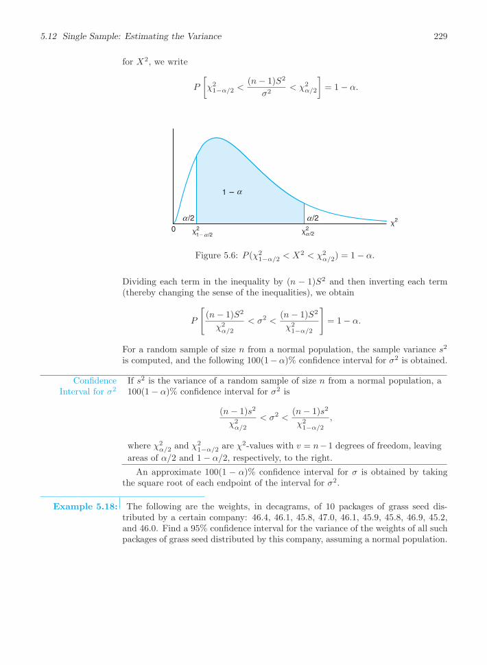
5.12 Single Sample: Estimating the Variance 229
for X2, we write
P
[χ21−α/2 <
(n− 1)S2
σ2< χ2
α/2
]= 1− α.
0 �21�
�2
�2/2
1 � α
α /2α
/2α
/2α
Figure 5.6: P (χ21−α/2 < X2 < χ2
α/2) = 1− α.
Dividing each term in the inequality by (n − 1)S2 and then inverting each term(thereby changing the sense of the inequalities), we obtain
P
[(n− 1)S2
χ2α/2
< σ2 <(n− 1)S2
χ21−α/2
]= 1− α.
For a random sample of size n from a normal population, the sample variance s2
is computed, and the following 100(1−α)% confidence interval for σ2 is obtained.
ConfidenceInterval for σ2
If s2 is the variance of a random sample of size n from a normal population, a100(1− α)% confidence interval for σ2 is
(n− 1)s2
χ2α/2
< σ2 <(n− 1)s2
χ21−α/2
,
where χ2α/2 and χ2
1−α/2 are χ2-values with v = n−1 degrees of freedom, leaving
areas of α/2 and 1− α/2, respectively, to the right.
An approximate 100(1 − α)% confidence interval for σ is obtained by takingthe square root of each endpoint of the interval for σ2.
Example 5.18: The following are the weights, in decagrams, of 10 packages of grass seed dis-tributed by a certain company: 46.4, 46.1, 45.8, 47.0, 46.1, 45.9, 45.8, 46.9, 45.2,and 46.0. Find a 95% confidence interval for the variance of the weights of all suchpackages of grass seed distributed by this company, assuming a normal population.

230 Chapter 5 One- and Two-Sample Estimation Problems
Solution : First we find
s2 =
nn∑
i=1
x2i −
(n∑
i=1
xi
)2
n(n− 1)
=(10)(21,273.12)− (461.2)2
(10)(9)= 0.286.
To obtain a 95% confidence interval, we choose α = 0.05. Then, using TableA.5 with v = 9 degrees of freedom, we find χ2
0.025 = 19.023 and χ20.975 = 2.700.
Therefore, the 95% confidence interval for σ2 is
(9)(0.286)
19.023< σ2 <
(9)(0.286)
2.700,
or simply 0.135 < σ2 < 0.953.
Exercises
5.54 A random sample of 20 students yielded a meanof x = 72 and a variance of s2 = 16 for scores on acollege placement test in mathematics. Assuming thescores to be normally distributed, construct a 98% con-fidence interval for σ2.
5.55 A manufacturer of car batteries claims that thebatteries will last, on average, 3 years with a varianceof 1 year. If 5 of these batteries have lifetimes of 1.9,2.4, 3.0, 3.5, and 4.2 years, construct a 95% confidenceinterval for σ2 and decide if the manufacturer’s claim
that σ2 = 1 is valid. Assume the population of batterylives to be approximately normally distributed.
5.56 Construct a 99% confidence interval for σ2 inCase Study 5.1 on page 211.
5.57 Construct a 95% confidence interval for σ2 inExercise 5.9 on page 213.
5.58 Construct a 90% confidence interval for σ in Ex-ercise 5.11 on page 213.
Review Exercises
5.59 According to the Roanoke Times, in a particu-lar year McDonald’s sold 42.1% of the market shareof hamburgers. A random sample of 75 burgers soldresulted in 28 of them being from McDonald’s. Usematerial in Section 5.10 to determine if this informa-tion supports the claim in the Roanoke Times.
5.60 It is claimed that a new diet will reduce a per-son’s weight by 4.5 kilograms on average in a periodof 2 weeks. The weights of 7 women who followed thisdiet were recorded before and after the 2-week period.Test the claim about the diet by computing a 95% con-fidence interval for the mean difference in weights. As-sume the differences of weights to be approximatelynormally distributed.
Woman Weight Before Weight After1 58.5 60.02 60.3 54.93 61.7 58.14 69.0 62.15 64.0 58.56 62.6 59.97 56.7 54.4
5.61 A health spa claims that a new exercise pro-gram will reduce a person’s waist size by 2 centimeterson average over a 5-day period. The waist sizes, incentimeters, of 6 men who participated in this exerciseprogram are recorded before and after the 5-day periodin the following table:

Review Exercises 231
Man Waist Size Before Waist Size After123456
90.495.598.7
115.9104.085.6
91.793.997.4
112.8101.384.0
By computing a 95% confidence interval for the meanreduction in waist size, determine whether the healthspa’s claim is valid. Assume the distribution of differ-ences in waist sizes before and after the program to beapproximately normal.
5.62 The Department of Civil Engineering at VirginiaTech compared a modified (M-5 hr) assay technique forrecovering fecal coliforms in stormwater runoff from anurban area to a most probable number (MPN) tech-nique. A total of 12 runoff samples were collected andanalyzed by the two techniques. Fecal coliform countsper 100 milliliters are recorded in the following table.
Sample MPN Count M-5 hr Count123456789
101112
23001200450210270450154179192230340194
2010930400436
41002090219169194174274183
Construct a 90% confidence interval for the differencein the mean fecal coliform counts between the M-5 hrand the MPN techniques. Assume that the count dif-ferences are approximately normally distributed.
5.63 An experiment was conducted to determinewhether surface finish has an effect on the endurancelimit of steel. There is a theory that polishing in-creases the average endurance limit (for reverse bend-ing). From a practical point of view, polishing shouldnot have any effect on the standard deviation of theendurance limit, which is known from numerous en-durance limit experiments to be 4000 psi. An ex-periment was performed on 0.4% carbon steel usingboth unpolished and polished smooth-turned speci-mens. The data are given below. Find a 95% con-fidence interval for the difference between the popu-lation means for the two methods, assuming that thepopulations are approximately normally distributed.
Endurance Limit (psi)
Polished Unpolished0.4% Carbon 0.4% Carbon
85,500 82,60091,900 82,40089,400 81,70084,000 79,50089,900 79,40078,700 69,80087,500 79,90083,100 83,400
5.64 An anthropologist is interested in the proportionof individuals in two Indian tribes with double occipi-tal hair whorls. Suppose that independent samples aretaken from each of the two tribes, and it is found that24 of 100 Indians from tribe A and 36 of 120 Indiansfrom tribe B possess this characteristic. Construct a95% confidence interval for the difference pB − pA be-tween the proportions of these two tribes with occipitalhair whorls.
5.65 A manufacturer of electric irons produces theseitems in two plants. Both plants have the same suppli-ers of small parts. A saving can be made by purchasingthermostats for plant B from a local supplier. A sin-gle lot was purchased from the local supplier, and atest was conducted to see whether or not these newthermostats were as accurate as the old. The ther-mostats were tested on tile irons on the 550◦F setting,and the actual temperatures were read to the nearest0.1◦F with a thermocouple. The data are as follows:
New Supplier (◦F)530.3 559.3 549.4 544.0 551.7 566.3549.9 556.9 536.7 558.8 538.8 543.3559.1 555.0 538.6 551.1 565.4 554.9550.0 554.9 554.7 536.1 569.1
Old Supplier (◦F)559.7 534.7 554.8 545.0 544.6 538.0550.7 563.1 551.1 553.8 538.8 564.6554.5 553.0 538.4 548.3 552.9 535.1555.0 544.8 558.4 548.7 560.3
Find 95% confidence intervals for σ21/σ
22 and for σ1/σ2,
where σ21 and σ2
2 are the population variances of thethermostat readings for the new and old suppliers, re-spectively.
5.66 It is argued that the resistance of wire A isgreater than the resistance of wire B. An experimenton the wires shows the results (in ohms) given here. As-suming equal variances, what conclusions do you draw?Justify your answer.

232 Chapter 5 One- and Two-Sample Estimation Problems
Wire A Wire B0.140 0.1350.138 0.1400.143 0.1360.142 0.1420.144 0.1380.137 0.140
5.67 A survey was done with the hope of comparingsalaries of chemical plant managers employed in twoareas of the country, the northern and west central re-gions. An independent random sample of 300 plantmanagers was selected from each of the two regions.These managers were asked their annual salaries. Theresults are as follows
North West Central
x1 = $102,300 x2 = $98,500s1 = $5700 s2 = $3800
(a) Construct a 99% confidence interval for μ1 − μ2,the difference in the mean salaries.
(b) What assumption did you make in (a) about thedistribution of annual salaries for the two regions?Is the assumption of normality necessary? Why orwhy not?
(c) What assumption did you make about the two vari-ances? Is the assumption of equality of variancesreasonable? Explain!
5.68 Consider Review Exercise 5.67. Let us assumethat the data have not been collected yet and that pre-vious statistics suggest that σ1 = σ2 = $4000. Arethe sample sizes in Review Exercise 5.67 sufficient toproduce a 95% confidence interval on μ1 −μ2 having awidth of only $1000? Show all work.
5.69 A labor union is becoming defensive about grossabsenteeism by its members. The union leaders hadalways claimed that, in a typical month, 95% of itsmembers were absent less than 10 hours. The uniondecided to check this by monitoring a random sampleof 300 of its members. The number of hours absentwas recorded for each of the 300 members. The resultswere x = 6.5 hours and s = 2.5 hours. Use the data torespond to this claim, using a one-sided tolerance limitand choosing the confidence level to be 99%. Be sureto interpret what you learn from the tolerance limitcalculation.
5.70 A random sample of 30 firms dealing in wirelessproducts was selected to determine the proportion ofsuch firms that have implemented new software to im-prove productivity. It turned out that 8 of the 30 hadimplemented such software. Find a 95% confidence in-terval on p, the true proportion of such firms that haveimplemented new software.
5.71 Refer to Review Exercise 5.70. Suppose there isconcern about whether the point estimate p = 8/30is accurate enough because the confidence intervalaround p is not sufficiently narrow. Using p as theestimate of p, how many companies would need to besampled in order to have a 95% confidence interval witha width of only 0.05?
5.72 A manufacturer turns out a product item that islabeled either “defective” or “not defective.” In orderto estimate the proportion defective, a random sam-ple of 100 items is taken from production, and 10 arefound to be defective. Following implementation of aquality improvement program, the experiment is con-ducted again. A new sample of 100 is taken, and thistime only 6 are found to be defective.
(a) Give a 95% confidence interval on p1 − p2, wherep1 is the population proportion defective before im-provement and p2 is the proportion defective afterimprovement.
(b) Is there information in the confidence intervalfound in (a) that would suggest that p1 > p2? Ex-plain.
5.73 A machine is used to fill boxes with productin an assembly line operation. Much concern centersaround the variability in the number of ounces of prod-uct in a box. The standard deviation in weight of prod-uct is known to be 0.3 ounce. An improvement is im-plemented, after which a random sample of 20 boxes isselected and the sample variance is found to be 0.045ounce2. Find a 95% confidence interval on the variancein the weight of the product. Does it appear from therange of the confidence interval that the improvementof the process enhanced quality as far as variability isconcerned? Assume normality on the distribution ofweights of product.
5.74 A consumer group is interested in comparingoperating costs for two different types of automobileengines. The group is able to find 15 owners whosecars have engine type A and 15 whose cars have enginetype B. All 30 owners bought their cars at roughly thesame time, and all have kept good records for a cer-tain 12-month period. In addition, these owners droveroughly the same number of miles. The cost statisticsare yA = $87.00/1000 miles, yB = $75.00/1000 miles,sA = $5.99, and sB = $4.85. Compute a 95% confi-dence interval to estimate μA − μB , the difference inthe mean operating costs. Assume normality and equalvariances.
5.75 A group of human factor researchers are con-cerned about reaction to a stimulus by airplane pilotsin a certain cockpit arrangement. An experiment wasconducted in a simulation laboratory, and 15 pilotswere used with average reaction time of 3.2 seconds

5.13 Potential Misconceptions and Hazards 233
with a sample standard deviation of 0.6 second. It isof interest to characterize the extreme (i.e., worst-casescenario). To that end, do the following:
(a) Give a particular important one-sided 99% confi-dence bound on the mean reaction time. Whatassumption, if any, must you make on the distribu-tion of reaction times?
(b) Give a 99% one-sided prediction interval and givean interpretation of what it means. Must you makean assumption about the distribution of reactiontimes to compute this bound?
(c) Compute a one-sided tolerance bound with 99%confidence that involves 95% of reaction times.Again, give an interpretation and assumptionsabout the distribution, if any. (Note: The one-sided tolerance limit values are also included in Ta-ble A.7.)
5.76 A certain supplier manufactures a type of rub-ber mat that is sold to automotive companies. Thematerial used to produce the mats must have certainhardness characteristics. Defective mats are occasion-ally discovered and rejected. The supplier claims thatthe proportion defective is 0.05. A challenge was madeby one of the clients who purchased the mats, so an ex-periment was conducted in which 400 mats were testedand 17 were found defective.
(a) Compute a 95% two-sided confidence interval onthe proportion defective.
(b) Compute an appropriate 95% one-sided confidenceinterval on the proportion defective.
(c) Interpret both intervals from (a) and (b) and com-ment on the claim made by the supplier.
5.13 Potential Misconceptions and Hazards;Relationship to Material in Other Chapters
The concept of a large-sample confidence interval on a population parameter isoften confusing to the beginning student. It is based on the notion that even whenσ is unknown and one is not convinced that the distribution being sampled isnormal, a confidence interval on μ can be computed from
x ± zα/2s√n.
In practice, this formula is often used when the sample is too small. The genesis ofthis large sample interval is, of course, the Central Limit Theorem (CLT), underwhich normality is not necessary in practice. Here the CLT requires a known σ,of which s is only an estimate. Thus, n must be at least as large as 30 and theunderlying distribution must be close to symmetric, in which case the intervalremains an approximation.
There are instances in which the appropriateness of the practical applicationof material in this chapter depends very much on the specific context. One veryimportant illustration is the use of the t-distribution for the confidence intervalon μ when σ is unknown. Strictly speaking, the use of the t-distribution requiresthat the distribution sampled from be normal. However, it is well known thatany application of the t-distribution is reasonably insensitive (i.e., robust) to thenormality assumption. This represents one of those fortunate situations whichoccur often in the field of statistics in which a basic assumption does not hold andyet “everything turns out all right!”
It is our experience that one of the most serious misuses of statistics in practiceevolves from confusion about distinctions in the interpretation of the types ofstatistical intervals. Thus, the subsection in this chapter where differences amongthe three types of intervals are discussed is important. It is very likely that inpractice the confidence interval is heavily overused. That is, it is used when

234 Chapter 5 One- and Two-Sample Estimation Problems
there is really no interest in the mean; rather, the question is “Where is the nextobservation going to fall?” or often, more importantly, “Where is the large bulk ofthe distribution?” These are crucial questions that are not answered by computingan interval on the mean.
The interpretation of a confidence interval is often misunderstood. It is tempt-ing to conclude that the parameter falls inside the interval with probability 0.95.A confidence interval merely suggests that if the experiment is conducted and dataare observed again and again, about 95% of such intervals will contain the trueparameter. Any beginning student of practical statistics should be very clear onthe difference among these statistical intervals.
Another potential serious misuse of statistics centers around the use of the χ2-distribution for a confidence interval on a single variance. Again, normality of thedistribution from which the sample is drawn is assumed. Unlike the use of thet-distribution, the use of the χ2 test for this application is not robust to the
normality assumption (i.e., the sampling distribution of (n−1)S2
σ2 deviates farfrom χ2 if the underlying distribution is not normal).

Chapter 6
One- and Two-SampleTests of Hypotheses
6.1 Statistical Hypotheses: General Concepts
Often, the problem confronting the scientist or engineer is not so much the es-timation of a population parameter, as discussed in Chapter 5, but rather theformation of a data-based decision procedure that can produce a conclusion aboutsome scientific system. For example, a medical researcher may decide on the basisof experimental evidence whether coffee drinking increases the risk of cancer inhumans; an engineer might have to decide on the basis of sample data whetherthere is a difference between the accuracy of two kinds of gauges; or a sociologistmight wish to collect appropriate data to enable him or her to decide whethera person’s blood type and eye color are independent variables. In each of thesecases, the scientist or engineer postulates or conjectures something about a system.In addition, each must make use of experimental data and make a decision basedon the data. In each case, the conjecture can be put in the form of a statisticalhypothesis. Procedures that lead to the acceptance or rejection of statistical hy-potheses such as these comprise a major area of statistical inference. First, let usdefine precisely what we mean by a statistical hypothesis.
Definition 6.1: A statistical hypothesis is an assertion or conjecture concerning one or morepopulations.
The truth or falsity of a statistical hypothesis is never known with absolutecertainty unless we examine the entire population. This, of course, would be im-practical in most situations. Instead, we take a random sample from the populationof interest and use the data contained in this sample to provide evidence that eithersupports or does not support the hypothesis. Evidence from the sample that isinconsistent with the stated hypothesis leads to a rejection of the hypothesis.
235

236 Chapter 6 One- and Two-Sample Tests of Hypotheses
The Role of Probability in Hypothesis Testing
It should be made clear to the reader that the decision procedure must include anawareness of the probability of a wrong conclusion. For example, suppose that thehypothesis postulated by the engineer is that the fraction defective p in a certainprocess is 0.10. The experiment is to observe a random sample of the productin question. Suppose that 100 items are tested and 12 items are found defective.It is reasonable to conclude that this evidence does not refute the condition thatthe binomial parameter p = 0.10, and thus it may lead one not to reject thehypothesis. However, it also does not refute p = 0.12 or perhaps even p = 0.15.As a result, the reader must be accustomed to understanding that rejection of ahypothesis implies that the sample evidence refutes it. Put another way,rejection means that there is a small probability of obtaining the sampleinformation observed when, in fact, the hypothesis is true. For example,for our proportion-defective hypothesis, a sample of 100 revealing 20 defective itemsis certainly evidence for rejection. Why? If, indeed, p = 0.10, the probability ofobtaining 20 or more defectives is approximately 0.002. With the resulting smallrisk of a wrong conclusion, it would seem safe to reject the hypothesis thatp = 0.10. In other words, rejection of a hypothesis tends to all but “rule out” thehypothesis. On the other hand, it is very important to emphasize that acceptanceor, rather, failure to reject does not rule out other possibilities. As a result, thefirm conclusion is established by the data analyst when a hypothesis is rejected.
The Null and Alternative Hypotheses
The structure of hypothesis testing will be formulated with the use of the termnull hypothesis, which refers to any hypothesis we wish to test and is denotedby H0. The rejection of H0 leads to the acceptance of an alternative hypoth-esis, denoted by H1. An understanding of the different roles played by the nullhypothesis (H0) and the alternative hypothesis (H1) is crucial to one’s understand-ing of the rudiments of hypothesis testing. The alternative hypothesis H1 usuallyrepresents the question to be answered or the theory to be tested, and thus its spec-ification is crucial. The null hypothesis H0 nullifies or opposes H1 and is often thelogical complement to H1. As the reader gains more understanding of hypothesistesting, he or she should note that the analyst arrives at one of the two followingconclusions:
reject H0 in favor of H1 because of sufficient evidence in the data or
fail to reject H0 because of insufficient evidence in the data.
Note that the conclusions do not involve a formal and literal “accept H0.” Thestatement of H0 often represents the “status quo” in opposition to the new idea,conjecture, and so on, stated in H1, while failure to reject H0 represents the properconclusion. In our binomial example, the practical issue may be a concern thatthe historical defective probability of 0.10 no longer is true. Indeed, the conjecturemay be that p exceeds 0.10. We may then state
H0: p = 0.10,
H1: p > 0.10.

6.2 Testing a Statistical Hypothesis 237
Now 12 defective items out of 100 does not refute p = 0.10, so the conclusion is“fail to reject H0.” However, if the data produce 20 out of 100 defective items,then the conclusion is “reject H0” in favor of H1: p > 0.10.
Though the applications of hypothesis testing are quite abundant in scientificand engineering work, perhaps the best illustration for a novice lies in the predica-ment encountered in a jury trial. The null and alternative hypotheses are
H0: defendant is not guilty,
H1: defendant is guilty.
The indictment comes because of suspicion of guilt. The hypothesis H0 (the statusquo) stands in opposition to H1 and is maintained unless H1 is supported byevidence “beyond a reasonable doubt.” However, “failure to reject H0” in this casedoes not imply innocence, but merely that the evidence was insufficient to convict.So the jury does not necessarily accept H0 but fails to reject H0.
6.2 Testing a Statistical Hypothesis
To illustrate the concepts used in testing a statistical hypothesis about a popula-tion, we present the following example. A certain type of cold vaccine is known tobe only 25% effective after a period of 2 years. To determine if a new and some-what more expensive vaccine is superior in providing protection against the samevirus for a longer period of time, suppose that 20 people are chosen at random andinoculated. (In an actual study of this type, the participants receiving the newvaccine might number several thousand. The number 20 is being used here onlyto demonstrate the basic steps in carrying out a statistical test.) If more than 8 ofthose receiving the new vaccine surpass the 2-year period without contracting thevirus, the new vaccine will be considered superior to the one presently in use. Therequirement that the number exceed 8 is somewhat arbitrary but appears reason-able in that it represents a modest gain over the 5 people who could be expected toreceive protection if the 20 people had been inoculated with the vaccine already inuse. We are essentially testing the null hypothesis that the new vaccine is equallyeffective after a period of 2 years as the one now commonly used. The alternativehypothesis is that the new vaccine is in fact superior. This is equivalent to testingthe hypothesis that the binomial parameter for the probability of a success on agiven trial is p = 1/4 against the alternative that p > 1/4. This is usually writtenas follows:
H0: p = 0.25,
H1: p > 0.25.
The Test Statistic
The test statistic on which we base our decision is X, the number of individualsin our test group who receive protection from the new vaccine for a period of atleast 2 years. The possible values of X, from 0 to 20, are divided into two groups:those numbers less than or equal to 8 and those greater than 8. All possible scores

238 Chapter 6 One- and Two-Sample Tests of Hypotheses
greater than 8 constitute the critical region. The last number that we observein passing into the critical region is called the critical value. In our illustration,the critical value is the number 8. Therefore, if x > 8, we reject H0 in favor of thealternative hypothesis H1. If x ≤ 8, we fail to reject H0. This decision criterion isillustrated in Figure 6.1.
0 1 2 3 4 5 6 7 8 9 10 11 12 13 14 15 16 17 18 19 20x
Do not reject H0(p � 0.25)
Reject H0(p 0.25)
Figure 6.1: Decision criterion for testing p = 0.25 versus p > 0.25.
The Probability of a Type I Error
The decision procedure just described could lead to either of two wrong conclusions.For instance, the new vaccine may be no better than the one now in use (H0 true)and yet, in this particular randomly selected group of individuals, more than 8surpass the 2-year period without contracting the virus. We would be committingan error by rejecting H0 in favor of H1 when, in fact, H0 is true. Such an error iscalled a type I error.
Definition 6.2: Rejection of the null hypothesis when it is true is called a type I error.
A second kind of error is committed if 8 or fewer of the group surpass the 2-yearperiod successfully and we are unable to conclude that the vaccine is better whenit actually is better (H1 true). Thus, in this case, we fail to reject H0 when in factH0 is false. This is called a type II error.
Definition 6.3: Nonrejection of the null hypothesis when it is false is called a type II error.
In testing any statistical hypothesis, there are four possible situations thatdetermine whether our decision is correct or in error. These four situations aresummarized in Table 6.1.
Table 6.1: Possible Situations for Testing a Statistical Hypothesis
H0 is true H0 is falseDo not reject H0 Correct decision Type II error
Reject H0 Type I error Correct decision
The probability of committing a type I error, also called the level of signif-icance, is denoted by the Greek letter α. In our illustration, a type I error willoccur when more than 8 individuals inoculated with the new vaccine surpass the2-year period without contracting the virus and researchers conclude that the newvaccine is better when it is actually equivalent to the one in use. Hence, if X is

6.2 Testing a Statistical Hypothesis 239
the number of individuals who remain free of the virus for at least 2 years,
α = P (type I error) = P
(X > 8 when p =
1
4
)=
20∑x=9
b
(x; 20,
1
4
)
= 1−8∑
x=0
b
(x; 20,
1
4
)= 1− 0.9591 = 0.0409.
We say that the null hypothesis, p = 1/4, is being tested at the α = 0.0409 level ofsignificance. Sometimes the level of significance is called the size of the test. Acritical region of size 0.0409 is very small, and therefore it is unlikely that a typeI error will be committed. Consequently, it would be most unusual for more than8 individuals to remain immune to a virus for a 2-year period using a new vaccinethat is essentially equivalent to the one now on the market.
The Probability of a Type II Error
The probability of committing a type II error, denoted by β, is impossible to com-pute unless we have a specific alternative hypothesis. If we test the null hypothesisthat p = 1/4 against the alternative hypothesis that p = 1/2, then we are ableto compute the probability of not rejecting H0 when it is false. We simply findthe probability of obtaining 8 or fewer in the group that surpass the 2-year periodwhen p = 1/2. In this case,
β = P (type II error) = P
(X ≤ 8 when p =
1
2
)=
8∑x=0
b
(x; 20,
1
2
)= 0.2517.
This is a rather high probability, indicating a test procedure in which it is quitelikely that we shall reject the new vaccine when, in fact, it is superior to what isnow in use. Ideally, we like to use a test procedure for which the type I and typeII error probabilities are both small.
It is possible that the director of the testing program is willing to make a typeII error if the more expensive vaccine is not significantly superior. In fact, the onlytime he wishes to guard against the type II error is when the true value of p is atleast 0.7. If p = 0.7, this test procedure gives
β = P (type II error) = P (X ≤ 8 when p = 0.7)
=8∑
x=0
b(x; 20, 0.7) = 0.0051.
With such a small probability of committing a type II error, it is extremely unlikelythat the new vaccine would be rejected when it was 70% effective after a period of2 years. As the alternative hypothesis approaches unity, the value of β diminishesto zero.

240 Chapter 6 One- and Two-Sample Tests of Hypotheses
The Role of α, β, and Sample Size
Let us assume that the director of the testing program is unwilling to commit atype II error when the alternative hypothesis p = 1/2 is true, even though we havefound the probability of such an error to be β = 0.2517. It is always possible toreduce β by increasing the size of the critical region. For example, consider whathappens to the values of α and β when we change our critical value to 7 so thatall scores greater than 7 fall in the critical region and those less than or equal to7 fall in the nonrejection region. Now, in testing p = 1/4 against the alternativehypothesis that p = 1/2, we find that
α =
20∑x=8
b
(x; 20,
1
4
)= 1−
7∑x=0
b
(x; 20,
1
4
)= 1− 0.8982 = 0.1018
and
β =7∑
x=0
b
(x; 20,
1
2
)= 0.1316.
By adopting a new decision procedure, we have reduced the probability of com-mitting a type II error at the expense of increasing the probability of committinga type I error. For a fixed sample size, a decrease in the probability of one errorwill usually result in an increase in the probability of the other error. Fortunately,the probability of committing both types of error can be reduced byincreasing the sample size. Consider the same problem using a random sampleof 100 individuals. If more than 36 of the group surpass the 2-year period, wereject the null hypothesis that p = 1/4 and accept the alternative hypothesis thatp > 1/4. The critical value is now 36. All possible scores above 36 constitute thecritical region, and all possible scores less than or equal to 36 fall in the acceptanceregion.
To determine the probability of committing a type I error, we shall use thenormal curve approximation with
μ = np = (100)
(1
4
)= 25 and σ =
√npq =
√(100)(1/4)(3/4) = 4.33.
Referring to Figure 6.2, we need the area under the normal curve to the right ofx = 36.5. The corresponding z-value is
z =36.5− 25
4.33= 2.66.
From Table A.3 we find that
α = P (type I error) = P
(X > 36 when p =
1
4
)≈ P (Z > 2.66)
= 1− P (Z < 2.66) = 1− 0.9961 = 0.0039.
If H0 is false and the true value of H1 is p = 1/2, we can determine theprobability of a type II error using the normal curve approximation with
μ = np = (100)(1/2) = 50 and σ =√npq =
√(100)(1/2)(1/2) = 5.

6.2 Testing a Statistical Hypothesis 241
xμ = 25 36.5
σ = 4.33
α
Figure 6.2: Probability of a type I error.
The probability of a value falling in the nonrejection region when H0 is false andH1 is true, with p = 1/2, is given by the area of the shaded region to the left ofx = 36.5 in Figure 6.3. The two normal distributions in the figure show the nullhypothesis on the left and the alternative hypothesis on the right. The z-valuecorresponding to x = 36.5 is
z =36.5− 50
5= −2.7.
x25 36.5 50
σ = 4.33 σ = 5
H0H1
Figure 6.3: Probability of a type II error.
Therefore,
β = P (type II error) = P
(X ≤ 36 when p =
1
2
)≈ P (Z < −2.7) = 0.0035.

242 Chapter 6 One- and Two-Sample Tests of Hypotheses
Obviously, the type I and type II errors will rarely occur if the experiment consistsof 100 individuals.
The illustration above underscores the strategy of the scientist in hypothesistesting. After the null and alternative hypotheses are stated, it is important toconsider the sensitivity of the test procedure. By this we mean that there shouldbe a determination, for a fixed α, of a reasonable value for the probability ofwrongly accepting H0 (i.e., the value of β) when the true situation represents someimportant deviation from H0. A value for the sample size can usually be determinedfor which there is a reasonable balance between the values of α and β computedin this fashion. The vaccine problem provides an illustration.
Illustration with a Continuous Random Variable
The concepts discussed here for a discrete population can be applied equally wellto continuous random variables. Consider the null hypothesis that the averageweight of male students in a certain college is 68 kilograms against the alternativehypothesis that it is unequal to 68. That is, we wish to test
H0: μ = 68,
H1: μ �= 68.
The alternative hypothesis allows for the possibility that μ < 68 or μ > 68.A sample mean that falls close to the hypothesized value of 68 would be consid-
ered evidence in favor ofH0. On the other hand, a sample mean that is considerablyless than or more than 68 would be evidence inconsistent with H0 and thereforefavoring H1. The sample mean is the test statistic in this case. A critical regionfor the test statistic might arbitrarily be chosen to be the two intervals x < 67and x > 69. The nonrejection region will then be the interval 67 ≤ x ≤ 69. Thisdecision criterion is illustrated in Figure 6.4.
67 68 69x
Reject H0( � 68)
Reject H0( � 68)
Do not reject H0( � 68)μ μμ
Figure 6.4: Critical region (in blue).
Let us now use the decision criterion of Figure 6.4 to calculate the probabilitiesof committing type I and type II errors when testing the null hypothesis thatμ = 68 kilograms against the alternative that μ �= 68 kilograms.
Assume the standard deviation of the population of weights to be σ = 3.6. Forlarge samples, we may substitute s for σ if no other estimate of σ is available.Our decision statistic, based on a random sample of size n = 36, will be X, themost efficient estimator of μ. From the Central Limit Theorem, we know thatthe sampling distribution of X is approximately normal with standard deviationσX = σ/
√n = 3.6/6 = 0.6.

6.2 Testing a Statistical Hypothesis 243
The probability of committing a type I error, or the level of significance of ourtest, is equal to the sum of the areas that have been shaded in each tail of thedistribution in Figure 6.5. Therefore,
α = P (X < 67 when μ = 68) + P (X > 69 when μ = 68).
x67 � 68 69
/2μ
α /2α
Figure 6.5: Critical region for testing μ = 68 versus μ �= 68.
The z-values corresponding to x1 = 67 and x2 = 69 when H0 is true are
z1 =67− 68
0.6= −1.67 and z2 =
69− 68
0.6= 1.67.
Therefore,
α = P (Z < −1.67) + P (Z > 1.67) = 2P (Z < −1.67) = 0.0950.
Thus, 9.5% of all samples of size 36 would lead us to reject μ = 68 kilograms when,in fact, it is true. To reduce α, we have a choice of increasing the sample sizeor widening the fail-to-reject region. Suppose that we increase the sample size ton = 64. Then σX = 3.6/8 = 0.45. Now
z1 =67− 68
0.45= −2.22 and z2 =
69− 68
0.45= 2.22.
Hence,
α = P (Z < −2.22) + P (Z > 2.22) = 2P (Z < −2.22) = 0.0264.
The reduction in α is not sufficient by itself to guarantee a good testing proce-dure. We must also evaluate β for various alternative hypotheses. If it is importantto reject H0 when the true mean is some value μ ≥ 70 or μ ≤ 66, then the prob-ability of committing a type II error should be computed and examined for thealternatives μ = 66 and μ = 70. Because of symmetry, it is only necessary toconsider the probability of not rejecting the null hypothesis that μ = 68 when thealternative μ = 70 is true. A type II error will result when the sample mean x fallsbetween 67 and 69 when H1 is true. Therefore, referring to Figure 6.6, we findthat
β = P (67 ≤ X ≤ 69 when μ = 70).

244 Chapter 6 One- and Two-Sample Tests of Hypotheses
67 68 69 70 71x
H0 H1
Figure 6.6: Probability of type II error for testing μ = 68 versus μ = 70.
The z-values corresponding to x1 = 67 and x2 = 69 when H1 is true are
z1 =67− 70
0.45= −6.67 and z2 =
69− 70
0.45= −2.22.
Therefore,
β = P (−6.67 < Z < −2.22) = P (Z < −2.22)− P (Z < −6.67)
= 0.0132− 0.0000 = 0.0132.
If the true value of μ is the alternative μ = 66, the value of β will again be0.0132. For all possible values of μ < 66 or μ > 70, the value of β will be evensmaller when n = 64, and consequently there would be little chance of not rejectingH0 when it is false.
The probability of committing a type II error increases rapidly when the truevalue of μ approaches, but is not equal to, the hypothesized value. Of course, thisis usually the situation where we do not mind making a type II error. For example,if the alternative hypothesis μ = 68.5 is true, we do not mind committing a typeII error by concluding that the true answer is μ = 68. The probability of makingsuch an error will be high when n = 64. Referring to Figure 6.7, we have
β = P (67 ≤ X ≤ 69 when μ = 68.5).
The z-values corresponding to x1 = 67 and x2 = 69 when μ = 68.5 are
z1 =67− 68.5
0.45= −3.33 and z2 =
69− 68.5
0.45= 1.11.
Therefore,
β = P (−3.33 < Z < 1.11) = P (Z < 1.11)− P (Z < −3.33)
= 0.8665− 0.0004 = 0.8661.

6.2 Testing a Statistical Hypothesis 245
67 68 6968.5x
H0 H1
Figure 6.7: Type II error for testing μ = 68 versus μ = 68.5.
One very important concept that relates to error probabilities is the notion ofthe power of a test.
Definition 6.4: The power of a test is the probability of rejecting H0 given that a specific alter-native is true.
The power of a test can be computed as 1 − β. Often different types oftests are compared by contrasting power properties. Consider the previousillustration, in which we were testing H0 : μ = 68 and H1 : μ �= 68. As before,suppose we are interested in assessing the sensitivity of the test. The test is gov-erned by the rule that we do not reject H0 if 67 ≤ x ≤ 69. We seek the capabilityof the test to properly reject H0 when indeed μ = 68.5. We have seen that theprobability of a type II error is given by β = 0.8661. Thus, the power of the testis 1 − 0.8661 = 0.1339. In a sense, the power is a more succinct measure of howsensitive the test is for detecting differences between a mean of 68 and a mean of68.5. In this case, if μ is truly 68.5, the test as described will properly reject H0
only 13.39% of the time. However, if μ = 70, the power of the test is 0.99, a verysatisfying value. From the foregoing, it is clear that to produce a desirable power(say, greater than 0.8), one must either increase α or increase the sample size.
So far in this chapter, much of the discussion of hypothesis testing has focusedon foundations and definitions. In the sections that follow, we get more specificand put hypotheses in categories as well as discuss tests of hypotheses on variousparameters of interest. We begin by drawing the distinction between a one-sidedand a two-sided hypothesis.
One- and Two-Tailed Tests
A test of any statistical hypothesis where the alternative is one sided, such as
H0: θ = θ0,
H1: θ > θ0

246 Chapter 6 One- and Two-Sample Tests of Hypotheses
or perhaps
H0: θ = θ0,
H1: θ < θ0,
is called a one-tailed test. Earlier in this section, we referred to the test statisticfor a hypothesis. Generally, the critical region for the alternative hypothesis θ > θ0lies in the right tail of the sampling distribution of the test statistic when the nullhypothesis is true, while the critical region for the alternative hypothesis θ < θ0 liesentirely in the left tail. (In a sense, the inequality symbol points in the directionof the critical region.) A one-tailed test was used in the vaccine experiment to testthe hypothesis p = 1/4 against the one-sided alternative p > 1/4 for the binomialdistribution.
A test of any statistical hypothesis where the alternative is two sided, such as
H0: θ = θ0,
H1: θ �= θ0,
is called a two-tailed test, since the critical region is split into two parts, oftenhaving equal probabilities, in each tail of the distribution of the test statistic. Thealternative hypothesis θ �= θ0 states that either θ < θ0 or θ > θ0. A two-tailedtest was used to test the null hypothesis that μ = 68 kilograms against the two-sided alternative μ �= 68 kilograms in the example of the continuous population ofstudent weights.
How Are the Null and Alternative Hypotheses Chosen?
The null hypothesis H0 will often be stated using the equality sign. With thisapproach, it is clear how the probability of type I error is controlled: just asshown in the preceding examples. However, there are situations in which “donot reject H0” implies that the parameter θ might be any value defined by thenatural complement to the alternative hypothesis. For example, in the vaccineexample, where the alternative hypothesis is H1: p > 1/4, it is quite possible thatnonrejection of H0 cannot rule out a value of p less than 1/4. Clearly though, inthe case of one-tailed tests, the statement of the alternative is the most importantconsideration.
Whether one sets up a one-tailed or a two-tailed test will depend on the con-clusion to be drawn if H0 is rejected. The location of the critical region can bedetermined only after H1 has been stated. For example, in testing a new drug, onesets up the hypothesis that it is no better than similar drugs now on the market andtests this against the alternative hypothesis that the new drug is superior. Suchan alternative hypothesis will result in a one-tailed test with the critical regionin the right tail. However, if we wish to compare a new teaching technique withthe conventional classroom procedure, the alternative hypothesis should allow forthe new approach to be either inferior or superior to the conventional procedure.Hence, the test is two-tailed with the critical region divided equally so as to fall inthe extreme left and right tails of the distribution of our statistic.

6.3 The Use of P -Values for Decision Making in Testing Hypotheses 247
Example 6.1: A manufacturer of a certain brand of rice cereal claims that the average saturatedfat content does not exceed 1.5 grams per serving. State the null and alternativehypotheses to be used in testing this claim and determine where the critical regionis located.
Solution : The manufacturer’s claim should be rejected only if μ is greater than 1.5 milligramsand should not be rejected if μ is less than or equal to 1.5 milligrams. We test
H0: μ = 1.5,
H1: μ > 1.5.
Nonrejection of H0 does not rule out values less than 1.5 milligrams. Since wehave a one-tailed test, the greater than symbol indicates that the critical regionlies entirely in the right tail of the distribution of our test statistic X.
Example 6.2: A real estate agent claims that 60% of all private residences being built today are3-bedroom homes. To test this claim, a large sample of new residences is inspected;the proportion of these homes with 3 bedrooms is recorded and used as the teststatistic. State the null and alternative hypotheses to be used in this test anddetermine the location of the critical region.
Solution : If the test statistic were substantially higher or lower than p = 0.6, we would rejectthe agent’s claim. Hence, we should make the hypothesis
H0: p = 0.6,
H1: p �= 0.6.
The alternative hypothesis implies a two-tailed test with the critical region dividedequally in both tails of the distribution of P , our test statistic.
6.3 The Use of P -Values for Decision Makingin Testing Hypotheses
In testing hypotheses in which the test statistic is discrete, the critical region maybe chosen arbitrarily and its size determined. If α is too large, it can be reducedby making an adjustment in the critical value. It may be necessary to increase thesample size to offset the decrease that occurs automatically in the power of thetest.
Preselection of a Significance Level
The preselection of a significance level α has its roots in the philosophy that themaximum risk of making a type I error should be controlled. However, this ap-proach does not account for values of test statistics that are “close” to the criticalregion. Suppose, for example, in the illustration withH0: μ = 10 versusH1: μ �= 10,a value of z = 1.87 is observed; strictly speaking, with α = 0.05, the value is notsignificant. But the risk of committing a type I error if one rejects H0 in this

248 Chapter 6 One- and Two-Sample Tests of Hypotheses
case could hardly be considered severe. In fact, in a two-tailed scenario, one canquantify this risk as
P = 2P (Z > 1.87 when μ = 10) = 2(0.0307) = 0.0614.
As a result, 0.0614 is the probability of obtaining a value of z as large as or larger(in magnitude) than 1.87 when in fact μ = 10. Although this evidence against H0
is not as strong as that which would result from rejection at an α = 0.05 level, itis important information to the user. Indeed, continued use of α = 0.05 or 0.01 isonly a result of what standards have been passed down through the generations.The P-value approach has been adopted extensively by users of appliedstatistics. The approach is designed to give the user an alternative (in termsof a probability) to a mere “reject” or “do not reject” conclusion. The P -valuecomputation also gives the user important information when the z-value falls wellinto the ordinary critical region. For example, if z is 2.73, it is informative for theuser to observe that
P = 2(0.0032) = 0.0064,
and thus the z-value is significant at a level considerably less than 0.05. It isimportant to know that under the condition of H0, a value of z = 2.73 is anextremely rare event. That is, a value at least that large in magnitude would onlyoccur 64 times in 10,000 experiments.
A Graphical Demonstration of a P-Value
One very simple way of explaining a P -value graphically is to consider two distinctsamples. Suppose that two materials are being considered for coating a particulartype of metal in order to inhibit corrosion. Specimens are obtained, and onecollection is coated with material 1 and one collection coated with material 2. Thesample sizes are n1 = n2 = 10, and corrosion is measured in percent of surfacearea affected. The hypothesis is that the samples came from common distributionswith mean μ = 10. Let us assume that the population variance is 1.0. Then weare testing
H0: μ1 = μ2 = 10.
Let Figure 6.8 represent a point plot of the data; the data are placed on thedistribution stated by the null hypothesis. Let us assume that the “×” data refer tomaterial 1 and the “◦” data refer to material 2. Now it seems clear that the data dorefute the null hypothesis. But how can this be summarized in one number? TheP-value can be viewed as simply the probability of obtaining these datagiven that both samples come from the same distribution. Clearly, thisprobability is quite small, say 0.00000001! Thus, the small P -value clearly refutesH0, and the conclusion is that the population means are significantly different.
Use of the P -value approach as an aid in decision-making is quite natural, andnearly all computer packages that provide hypothesis-testing computation printout P -values along with values of the appropriate test statistic. The following is aformal definition of a P -value.
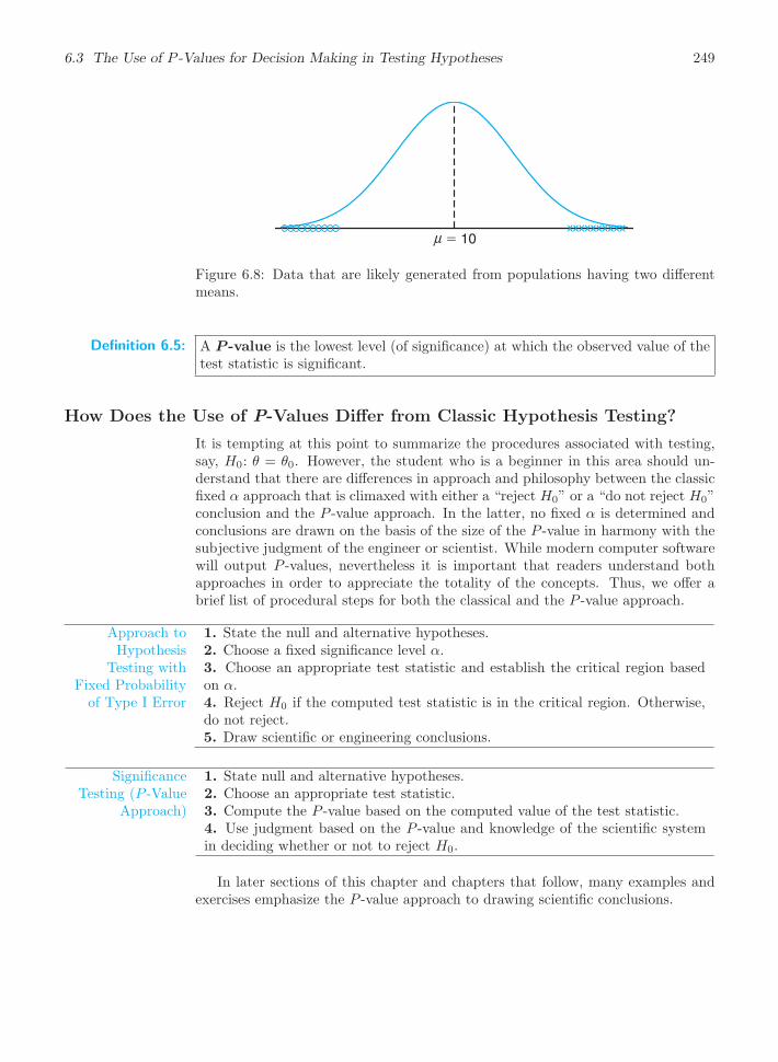
6.3 The Use of P -Values for Decision Making in Testing Hypotheses 249
� 10μ
Figure 6.8: Data that are likely generated from populations having two differentmeans.
Definition 6.5: A P -value is the lowest level (of significance) at which the observed value of thetest statistic is significant.
How Does the Use of P-Values Differ from Classic Hypothesis Testing?
It is tempting at this point to summarize the procedures associated with testing,say, H0: θ = θ0. However, the student who is a beginner in this area should un-derstand that there are differences in approach and philosophy between the classicfixed α approach that is climaxed with either a “reject H0” or a “do not reject H0”conclusion and the P -value approach. In the latter, no fixed α is determined andconclusions are drawn on the basis of the size of the P -value in harmony with thesubjective judgment of the engineer or scientist. While modern computer softwarewill output P -values, nevertheless it is important that readers understand bothapproaches in order to appreciate the totality of the concepts. Thus, we offer abrief list of procedural steps for both the classical and the P -value approach.
Approach toHypothesis
Testing withFixed Probabilityof Type I Error
1. State the null and alternative hypotheses.2. Choose a fixed significance level α.3. Choose an appropriate test statistic and establish the critical region basedon α.4. Reject H0 if the computed test statistic is in the critical region. Otherwise,do not reject.5. Draw scientific or engineering conclusions.
SignificanceTesting (P -Value
Approach)
1. State null and alternative hypotheses.2. Choose an appropriate test statistic.3. Compute the P -value based on the computed value of the test statistic.4. Use judgment based on the P -value and knowledge of the scientific systemin deciding whether or not to reject H0.
In later sections of this chapter and chapters that follow, many examples andexercises emphasize the P -value approach to drawing scientific conclusions.

250 Chapter 6 One- and Two-Sample Tests of Hypotheses
Exercises
6.1 Suppose that an allergist wishes to test the hy-pothesis that at least 30% of the public is allergic tosome cheese products. Explain how the allergist couldcommit
(a) a type I error;
(b) a type II error.
6.2 A sociologist is concerned about the effectivenessof a training course designed to get more drivers to useseat belts in automobiles.
(a) What hypothesis is she testing if she commits atype I error by erroneously concluding that thetraining course is ineffective?
(b) What hypothesis is she testing if she commits atype II error by erroneously concluding that thetraining course is effective?
6.3 A large manufacturing firm is being charged withdiscrimination in its hiring practices.
(a) What hypothesis is being tested if a jury commitsa type I error by finding the firm guilty?
(b) What hypothesis is being tested if a jury commitsa type II error by finding the firm guilty?
6.4 A fabric manufacturer believes that the propor-tion of orders for raw material arriving late is p = 0.6.If a random sample of 10 orders shows that 3 or fewerarrived late, the hypothesis that p = 0.6 should berejected in favor of the alternative p < 0.6. Use thebinomial distribution.
(a) Find the probability of committing a type I errorif the true proportion is p = 0.6.
(b) Find the probability of committing a type II errorfor the alternatives p = 0.3, p = 0.4, and p = 0.5.
6.5 Repeat Exercise 6.4 but assume that 50 orders areselected and the critical region is defined to be x ≤ 24,where x is the number of orders in the sample thatarrived late. Use the normal approximation.
6.6 The proportion of adults living in a small townwho are college graduates is estimated to be p = 0.6.To test this hypothesis, a random sample of 15 adultsis selected. If the number of college graduates in thesample is anywhere from 6 to 12, we shall not rejectthe null hypothesis that p = 0.6; otherwise, we shallconclude that p = 0.6.
(a) Evaluate α assuming that p = 0.6. Use the bino-mial distribution.
(b) Evaluate β for the alternatives p = 0.5 and p = 0.7.
(c) Is this a good test procedure?
6.7 Repeat Exercise 6.6 but assume that 200 adultsare selected and the fail-to-reject region is defined tobe 110 ≤ x ≤ 130, where x is the number of collegegraduates in our sample. Use the normal approxima-tion.
6.8 In Relief from Arthritis published by ThorsonsPublishers, Ltd., John E. Croft claims that over 40%of those who suffer from osteoarthritis receive measur-able relief from an ingredient produced by a particularspecies of mussel found off the coast of New Zealand.To test this claim, the mussel extract is to be given toa group of 7 osteoarthritic patients. If 3 or more ofthe patients receive relief, we shall not reject the nullhypothesis that p = 0.4; otherwise, we shall concludethat p < 0.4.
(a) Evaluate α, assuming that p = 0.4.
(b) Evaluate β for the alternative p = 0.3.
6.9 A dry cleaning establishment claims that a newspot remover will remove more than 70% of the spotsto which it is applied. To check this claim, the spotremover will be used on 12 spots chosen at random. Iffewer than 11 of the spots are removed, we shall notreject the null hypothesis that p = 0.7; otherwise, weshall conclude that p > 0.7.
(a) Evaluate α, assuming that p = 0.7.
(b) Evaluate β for the alternative p = 0.9.
6.10 Repeat Exercise 6.9 but assume that 100 spotsare treated and the critical region is defined to bex > 82, where x is the number of spots removed.
6.11 Repeat Exercise 6.8 but assume that 70 patientsare given the mussel extract and the critical region isdefined to be x < 24, where x is the number of os-teoarthritic patients who receive relief.
6.12 A random sample of 400 voters in a certain cityare asked if they favor an additional 4% gasoline salestax to provide badly needed revenues for street repairs.If more than 220 but fewer than 260 favor the sales tax,we shall conclude that 60% of the voters are for it.
(a) Find the probability of committing a type I errorif 60% of the voters favor the increased tax.
(b) What is the probability of committing a type II er-ror using this test procedure if actually only 48%of the voters are in favor of the additional gasolinetax?
6.13 Suppose, in Exercise 6.12, we conclude that 60%of the voters favor the gasoline sales tax if more than214 but fewer than 266 voters in our sample favor it.Show that this new critical region results in a smallervalue for α at the expense of increasing β.

6.4 Single Sample: Tests Concerning a Single Mean 251
6.14 A manufacturer has developed a new fishingline, which the company claims has a mean breakingstrength of 15 kilograms with a standard deviation of0.5 kilogram. To test the hypothesis that μ = 15 kilo-grams against the alternative that μ < 15 kilograms, arandom sample of 50 lines will be tested. The criticalregion is defined to be x < 14.9.
(a) Find the probability of committing a type I errorwhen H0 is true.
(b) Evaluate β for the alternatives μ = 14.8 and μ =14.9 kilograms.
6.15 A soft-drink machine at a steak house is reg-ulated so that the amount of drink dispensed is ap-proximately normally distributed with a mean of 200milliliters and a standard deviation of 15 milliliters.The machine is checked periodically by taking a sam-ple of 9 drinks and computing the average content. Ifx falls in the interval 191 < x < 209, the machine isthought to be operating satisfactorily; otherwise, weconclude that μ = 200 milliliters.
(a) Find the probability of committing a type I errorwhen μ = 200 milliliters.
(b) Find the probability of committing a type II errorwhen μ = 215 milliliters.
6.16 Repeat Exercise 6.15 for samples of size n = 25.
Use the same critical region.
6.17 A new curing process developed for a certaintype of cement results in a mean compressive strengthof 5000 kilograms per square centimeter with a stan-dard deviation of 120 kilograms per square centimeter.To test the hypothesis that μ = 5000 against the al-ternative that μ < 5000, a random sample of 50 piecesof cement is tested. The critical region is defined to bex < 4970.
(a) Find the probability of committing a type I errorwhen H0 is true.
(b) Evaluate β for the alternatives μ = 4970 andμ = 4960.
6.18 If we plot the probabilities of failing to reject H0
corresponding to various alternatives for μ (includingthe value specified by H0) and connect all the pointsby a smooth curve, we obtain the operating charac-teristic curve of the test criterion, or the OC curve.Note that the probability of failing to reject H0 when itis true is simply 1−α. Operating characteristic curvesare widely used in industrial applications to provide avisual display of the merits of the test criterion. Withreference to Exercise 6.15, find the probabilities of fail-ing to reject H0 for the following 9 values of μ and plotthe OC curve: 184, 188, 192, 196, 200, 204, 208, 212,and 216.
6.4 Single Sample: Tests Concerning a Single Mean
In this section, we formally consider tests of hypotheses on a single populationmean. Many of the illustrations from previous sections involved tests on the mean,so the reader should already have insight into some of the details that are outlinedhere.
Tests on a Single Mean (Variance Known)
We should first describe the assumptions on which the experiment is based. Themodel for the underlying situation centers around an experiment with X1, X2, . . . ,Xn representing a random sample from a distribution with mean μ and varianceσ2 > 0. Consider first the hypothesis
H0: μ = μ0,
H1: μ �= μ0.
The appropriate test statistic should be based on the random variable X. InChapter 4, the Central Limit Theorem was introduced, which essentially statesthat despite the distribution of X, the random variable X has approximately anormal distribution with mean μ and variance σ2/n for reasonably large samplesizes. So, μX = μ and σ2
X= σ2/n. We can then determine a critical region based

252 Chapter 6 One- and Two-Sample Tests of Hypotheses
on the computed sample average, x. It should be clear to the reader by now thatthere will be a two-tailed critical region for the test.
Standardization of X
It is convenient to standardize X and formally involve the standard normalrandom variable Z, where
Z =X − μ
σ/√n.
We know that under H0, the Central Limit Theorem states that μX = μ0,√n(X−
μ0)/σ follows an n(x; 0, 1) distribution. Hence Z will fall between the critical values−zα/2 and zα/2 with a probability of 1− α. The expression
P
(−zα/2 <
X − μ0
σ/√n
< zα/2
)= 1− α
can be used to write an appropriate nonrejection region. The reader should keepin mind that, formally, the critical region is designed to control α, the probabilityof a type I error. It should be obvious that a two-tailed signal of evidence is neededto support H1. Thus, given a computed value x, the formal test involves rejectingH0 if the computed test statistic z falls in the critical region described next.
Test Procedurefor a Single Mean
(VarianceKnown)
z =x− μ0
σ/√n
> zα/2 or z =x− μ0
σ/√n
< −zα/2
If −zα/2 < z < zα/2, do not reject H0. Rejection of H0, of course, impliesacceptance of the alternative hypothesis μ �= μ0. With this definition of thecritical region, it should be clear that there will be probability α of rejecting H0
(falling into the critical region) when, indeed, μ = μ0.
Although it is easier to understand the critical region written in terms of z,we can write the same critical region in terms of the computed average x. Thefollowing can be written as an identical decision procedure:
reject H0 if x < a or x > b,
where
a = μ0 − zα/2σ√n, b = μ0 + zα/2
σ√n.
Hence, for a significance level α, the critical values of the random variable z and xare both depicted in Figure 6.9.
Tests of one-sided hypotheses on the mean involve the same statistic describedin the two-sided case. The difference, of course, is that the critical region is onlyin one tail of the standard normal distribution. For example, suppose that we seekto test
H0: μ = μ0,
H1: μ > μ0.

6.4 Single Sample: Tests Concerning a Single Mean 253
xa μ b
1 �
/2
α
α /2α
Figure 6.9: Critical region for the alternative hypothesis μ �= μ0.
The signal that favorsH1 comes from large values of z. Thus, rejection ofH0 resultswhen the computed z > zα. Obviously, if the alternative is H1: μ < μ0, the criticalregion is entirely in the lower tail and thus rejection results from z < −zα. Althoughin a one-sided testing case the null hypothesis can be written as H0 : μ ≤ μ0 orH0: μ ≥ μ0, it is usually written as H0: μ = μ0.
The following two examples illustrate tests on means for the case in which σ isknown.
Example 6.3: A random sample of 100 recorded deaths in the United States during the pastyear showed an average life span of 71.8 years. Assuming a population standarddeviation of 8.9 years, does this seem to indicate that the mean life span today isgreater than 70 years? Use a 0.05 level of significance.
Solution : 1. H0: μ = 70 years.
2. H1: μ > 70 years.
3. α = 0.05.
4. Critical region: z > 1.645, where z = x−μ0
σ/√n.
5. Computations: x = 71.8 years, σ = 8.9 years, and hence z = 71.8−708.9/
√100
= 2.02.
6. Decision: Reject H0 and conclude that the mean life span today is greaterthan 70 years.
The P -value corresponding to z = 2.02 is given by the area of the shaded regionin Figure 6.10.
Using Table A.3, we have
P = P (Z > 2.02) = 0.0217.
As a result, the evidence in favor of H1 is even stronger than that suggested by a0.05 level of significance.
Example 6.4: Amanufacturer of sports equipment has developed a new synthetic fishing line thatthe company claims has a mean breaking strength of 8 kilograms with a standarddeviation of 0.5 kilogram. Test the hypothesis that μ = 8 kilograms against thealternative that μ �= 8 kilograms if a random sample of 50 lines is tested and foundto have a mean breaking strength of 7.8 kilograms. Use a 0.01 level of significance.

254 Chapter 6 One- and Two-Sample Tests of Hypotheses
z0 2.02
P
Figure 6.10: P -value for Example 6.3.
z−2.83 0 2.83
P /2 P /2
Figure 6.11: P -value for Example 6.4.
Solution : 1. H0: μ = 8 kilograms.
2. H1: μ �= 8 kilograms.
3. α = 0.01.
4. Critical region: z < −2.575 and z > 2.575, where z = x−μ0
σ/√n.
5. Computations: x = 7.8 kilograms, n = 50, and hence z = 7.8−80.5/
√50
= −2.83.
6. Decision: Reject H0 and conclude that the average breaking strength is notequal to 8.
Since the test in this example is two tailed, the desired P -value is twice thearea of the shaded region in Figure 6.11 to the left of z = −2.83. Therefore, usingTable A.3, we have
P = P (|Z| > 2.83) = 2P (Z < −2.83) = 0.0046,
which allows us to reject the null hypothesis that μ = 8 kilograms at a level ofsignificance smaller than 0.01.
Relationship to Confidence Interval Estimation
The reader should realize by now that the hypothesis-testing approach to statisticalinference in this chapter is very closely related to the confidence interval approach inChapter 5. Confidence interval estimation involves computation of bounds withinwhich it is “reasonable” for the parameter in question to lie. For the case of asingle population mean μ with σ2 known, the structure of both hypothesis testingand confidence interval estimation is based on the random variable
Z =X − μ
σ/√n.
It turns out that the testing of H0: μ = μ0 against H1: μ �= μ0 at a significance levelα is equivalent to computing a 100(1− α)% confidence interval on μ and rejectingH0 if μ0 is outside the confidence interval. If μ0 is inside the confidence interval,the hypothesis is not rejected. The equivalence is very intuitive and quite simple to

6.4 Single Sample: Tests Concerning a Single Mean 255
illustrate. Recall that with an observed value x, failure to reject H0 at significancelevel α implies that
−zα/2 ≤ x− μ0
σ/√n
≤ zα/2,
which is equivalent to
x− zα/2σ√n≤ μ0 ≤ x+ zα/2
σ√n.
The equivalence of confidence interval estimation to hypothesis testing extendsto differences between two means, variances, ratios of variances, and so on. As aresult, the student of statistics should not consider confidence interval estimationand hypothesis testing as separate forms of statistical inference.
Tests on a Single Sample (Variance Unknown)
One would certainly suspect that tests on a population mean μ with σ2 unknown,like confidence interval estimation, should involve use of the Student t-distribution.Strictly speaking, the application of Student t for both confidence intervals andhypothesis testing is developed under the following assumptions. The randomvariables X1, X2, . . . , Xn represent a random sample from a normal distributionwith unknown μ and σ2. Then the random variable
√n(X − μ)/S has a Student
t-distribution with n−1 degrees of freedom. The structure of the test is identical tothat for the case of σ known, with the exception that the value σ in the test statisticis replaced by the computed estimate S and the standard normal distribution isreplaced by a t-distribution.
The t-Statisticfor a Test on a
Single Mean(VarianceUnknown)
For the two-sided hypothesis
H0: μ = μ0,
H1: μ �= μ0,
we reject H0 at significance level α when the computed t-statistic
t =x− μ0
s/√n
exceeds tα/2,n−1 or is less than −tα/2,n−1.
The reader should recall from Chapters 4 and 5 that the t-distribution is symmetricaround the value zero. Thus, this two-tailed critical region applies in a fashionsimilar to that for the case of known σ. For the two-sided hypothesis at significancelevel α, the two-tailed critical regions apply. For H1: μ > μ0, rejection results whent > tα,n−1. For H1: μ < μ0, the critical region is given by t < −tα,n−1.
Example 6.5: The Edison Electric Institute has published figures on the number of kilowatt hoursused annually by various home appliances. It is claimed that a vacuum cleaner usesan average of 46 kilowatt hours per year. If a random sample of 12 homes included

256 Chapter 6 One- and Two-Sample Tests of Hypotheses
in a planned study indicates that vacuum cleaners use an average of 42 kilowatthours per year with a sample standard deviation of 11.9 kilowatt hours, does thissuggest at the 0.05 level of significance that vacuum cleaners use, on average, lessthan 46 kilowatt hours annually? Assume the population of kilowatt hours to benormal.
Solution : 1. H0: μ = 46 kilowatt hours.
2. H1: μ < 46 kilowatt hours.
3. α = 0.05.
4. Critical region: t < −1.796, where t = x−μ0
s/√nwith 11 degrees of freedom.
5. Computations: x = 42 kilowatt hours, s = 11.9 kilowatt hours, and n = 12.Hence,
t =42− 46
11.9/√12
= −1.16, P = P (T < −1.16) ≈ 0.135.
6. Decision: Do not reject H0 and conclude that the average number of kilowatthours used annually by home vacuum cleaners is not significantly less than46.
Comment on the Single-Sample t-Test
Comments regarding the normality assumption are worth emphasizing at thispoint. We have indicated that when σ is known, the Central Limit Theoremallows for the use of a test statistic or a confidence interval which is based on Z,the standard normal random variable. Strictly speaking, of course, the CentralLimit Theorem, and thus the use of the standard normal distribution, does notapply unless σ is known. In Chapter 4, the development of the t-distribution wasgiven. There we pointed out that normality on X1, X2, . . . , Xn was an underlyingassumption. Thus, strictly speaking, the Student’s t-tables of percentage points fortests or confidence intervals should not be used unless it is known that the samplecomes from a normal population. In practice, σ can rarely be assumed to be known.However, a very good estimate may be available from previous experiments. Manystatistics textbooks suggest that one can safely replace σ by s in the test statistic
z =x− μ0
σ/√n
when n ≥ 30 with a bell-shaped population and still use the Z-tables for theappropriate critical region. The implication here is that the Central Limit Theoremis indeed being invoked and one is relying on the fact that s ≈ σ. Obviously, whenthis is done, the results must be viewed as approximate. Thus, a computed P -value (from the Z-distribution) of 0.15 may be 0.12 or perhaps 0.17, or a computedconfidence interval may be a 93% confidence interval rather than a 95% intervalas desired. Now what about situations where n ≤ 30? The user cannot rely on sbeing close to σ, and in order to take into account the inaccuracy of the estimate,the confidence interval should be wider or the critical value larger in magnitude.The t-distribution percentage points accomplish this but are correct only when the

6.4 Single Sample: Tests Concerning a Single Mean 257
sample is from a normal distribution. Of course, normal probability plots can beused to ascertain some sense of the deviation from normality in a data set.
For small samples, it is often difficult to detect deviations from a normal dis-tribution. (Goodness-of-fit tests are discussed in a later section of this chapter.)For bell-shaped distributions of the random variables X1, X2, . . . , Xn, the use ofthe t-distribution for tests or confidence intervals is likely to produce quite goodresults. When in doubt, the user should resort to nonparametric procedures.
Annotated Computer Printout for Single-Sample t-Test
It should be of interest for the reader to see an annotated computer printoutshowing the result of a single-sample t-test. Suppose that an engineer is interestedin testing the bias in a pH meter. Data are collected on a neutral substance (pH= 7.0). A sample of the measurements is taken, with the data as follows:
7.07 7.00 7.10 6.97 7.00 7.03 7.01 7.01 6.98 7.08
It is, then, of interest to test
H0: μ = 7.0,
H1: μ �= 7.0.
In this illustration, we use the computer package MINITAB to illustrate the anal-ysis of the data set above. Notice the key components of the printout shown inFigure 6.12. The mean y is 7.0250, StDev is simply the sample standard devia-tion s = 0.044, and SE Mean is the estimated standard error of the mean and iscomputed as s/
√n = 0.0139. The t-value is the ratio
(7.0250− 7)/0.0139 = 1.80.
pH-meter
7.07 7.00 7.10 6.97 7.00 7.03 7.01 7.01 6.98 7.08
MTB > Onet ’pH-meter’; SUBC> Test 7.
One-Sample T: pH-meter Test of mu = 7 vs not = 7
Variable N Mean StDev SE Mean 95% CI T P
pH-meter 10 7.02500 0.04403 0.01392 (6.99350, 7.05650) 1.80 0.106
Figure 6.12: MINITAB printout for one-sample t-test for pH meter.
The P -value of 0.106 suggests results that are inconclusive. There is no evi-dence suggesting a strong rejection of H0 (based on an α of 0.05 or 0.10), yet onecertainly cannot confidently conclude that the pH meter is unbiased.Notice that the sample size of 10 is rather small. An increase in sample size (per-haps another experiment) may sort things out. A discussion regarding appropriatesample size appears in Section 6.6.

258 Chapter 6 One- and Two-Sample Tests of Hypotheses
6.5 Two Samples: Tests on Two Means
The reader should now understand the relationship between tests and confidenceintervals, and can rely on details supplied by the confidence interval material inChapter 5. Tests concerning two means represent a set of very important analyticaltools for the scientist or engineer. The experimental setting is very much like thatdescribed in Section 5.8. Two independent random samples of sizes n1 and n2,respectively, are drawn from two populations with means μ1 and μ2 and variancesσ21 and σ2
2 . We know that the random variable
Z =(X1 − X2)− (μ1 − μ2)√
σ21/n1 + σ2
2/n2
has a standard normal distribution. Here we are assuming that n1 and n2 aresufficiently large that the Central Limit Theorem applies. Of course, if the twopopulations are normal, the statistic above has a standard normal distributioneven for small n1 and n2. Obviously, if we can assume that σ1 = σ2 = σ, thestatistic above reduces to
Z =(X1 − X2)− (μ1 − μ2)
σ√1/n1 + 1/n2
.
The two statistics above serve as a basis for the development of the test proceduresinvolving two means. The equivalence between tests and confidence intervals, alongwith the technical detail involving tests on one mean, allows a simple transition totests on two means.
The two-sided hypothesis on two means can be written generally as
H0: μ1 − μ2 = d0.
Obviously, the alternative can be two sided or one sided. Again, the distribu-tion used is the distribution of the test statistic under H0. Values x1 and x2 arecomputed and, for σ1 and σ2 known, the test statistic is given by
z =(x1 − x2)− d0√σ21/n1 + σ2
2/n2
,
with a two-tailed critical region in the case of a two-sided alternative. That is,reject H0 in favor of H1: μ1 −μ2 �= d0 if z > zα/2 or z < −zα/2. One-tailed criticalregions are used in the case of the one-sided alternatives. The reader should, asbefore, study the test statistic and be satisfied that for, say, H1: μ1 − μ2 > d0, thesignal favoring H1 comes from large values of z. Thus, the upper-tailed criticalregion applies.
Unknown but Equal Variances
The more prevalent situations involving tests on two means are those in whichvariances are unknown. If the scientist involved is willing to assume that bothdistributions are normal and that σ1 = σ2 = σ, the pooled t-test (often called thetwo-sample t-test) may be used. The test statistic (see Section 5.8) is given by thefollowing test procedure.

6.5 Two Samples: Tests on Two Means 259
Two-SamplePooled t-Test
For the two-sided hypothesis
H0: μ1 = μ2,
H1: μ1 �= μ2,
we reject H0 at significance level α when the computed t-statistic
t =(x1 − x2)− d0
sp√
1/n1 + 1/n2
,
where
s2p =s21(n1 − 1) + s22(n2 − 1)
n1 + n2 − 2,
exceeds tα/2,n1+n2−2 or is less than −tα/2,n1+n2−2.
Recall from Chapter 5 that the degrees of freedom for the t-distribution are aresult of pooling of information from the two samples to estimate σ2. One-sidedalternatives suggest one-sided critical regions, as one might expect. For example,for H1: μ1 − μ2 > d0, reject H1: μ1 − μ2 = d0 when t > tα,n1+n2−2.
Example 6.6: An experiment was performed to compare the abrasive wear of two different lami-nated materials. Twelve pieces of material 1 were tested by exposing each piece toa machine measuring wear. Ten pieces of material 2 were similarly tested. In eachcase, the depth of wear was observed. The samples of material 1 gave an average(coded) wear of 85 units with a sample standard deviation of 4, while the samplesof material 2 gave an average of 81 with a sample standard deviation of 5. Canwe conclude at the 0.05 level of significance that the abrasive wear of material 1exceeds that of material 2 by more than 2 units? Assume the populations to beapproximately normal with equal variances.
Solution : Let μ1 and μ2 represent the population means of the abrasive wear for material 1and material 2, respectively.
1. H0: μ1 − μ2 = 2.
2. H1: μ1 − μ2 > 2.
3. α = 0.05.
4. Critical region: t > 1.725, where t = (x1−x2)−d0
sp√
1/n1+1/n2
with v = 20 degrees of
freedom.
5. Computations:
x1 = 85, s1 = 4, n1 = 12,
x2 = 81, s2 = 5, n2 = 10.

260 Chapter 6 One- and Two-Sample Tests of Hypotheses
Hence
sp =
√(11)(16) + (9)(25)
12 + 10− 2= 4.478,
t =(85− 81)− 2
4.478√1/12 + 1/10
= 1.04,
P = P (T > 1.04) ≈ 0.16. (See Table A.4.)
6. Decision: Do not reject H0. We are unable to conclude that the abrasive wearof material 1 exceeds that of material 2 by more than 2 units.
Unknown but Unequal Variances
There are situations where the analyst is not able to assume that σ1 = σ2. Recallfrom Section 5.8 that, if the populations are normal, the statistic
T ′ =(X1 − X2)− d0√s21/n1 + s22/n2
has an approximate t-distribution with approximate degrees of freedom
v =(s21/n1 + s22/n2)
2
(s21/n1)2/(n1 − 1) + (s22/n2)2/(n2 − 1).
As a result, the test procedure is to not reject H0 when
−tα/2,v < t′ < tα/2,v,
with v given as above. Again, as in the case of the pooled t-test, one-sided alterna-tives suggest one-sided critical regions. The test procedures developed above aresummarized in Table 6.3.
Paired Observations
A study of the two-sample t-test or confidence interval on the difference betweenmeans should suggest the need for an experimental design. Recall the discussionof experimental units in Chapter 5, where it was suggested that the conditions ofthe two populations (often referred to as the two treatments) should be assignedrandomly to the experimental units. This is done to avoid biased results due tosystematic differences between experimental units. In other words, in hypothesis-testing jargon, it is important that any significant difference found between meansbe due to the different conditions of the populations and not due to the exper-imental units in the study. For example, consider Exercise 5.28 in Section 5.9.The 20 seedlings play the role of the experimental units. Ten of them are to betreated with nitrogen and 10 not treated with nitrogen. It may be very importantthat this assignment to the “nitrogen” and “no-nitrogen” treatments be randomto ensure that systematic differences between the seedlings do not interfere with avalid comparison between the means.

6.5 Two Samples: Tests on Two Means 261
In Example 6.6, time of measurement is the most likely choice for the experi-mental unit. The 22 pieces of material should be measured in random order. Weneed to guard against the possibility that wear measurements made close togetherin time might tend to give similar results. Systematic (nonrandom) differencesin experimental units are not expected. However, random assignments guardagainst the problem.
References to planning of experiments, randomization, choice of sample size,and so on, will continue to influence much of the development in Chapter 8. Anyscientist or engineer whose interest lies in analysis of real data should study thismaterial. The pooled t-test is extended in Chapter 8 to cover more than two means.
Testing of two means can be accomplished when data are in the form of pairedobservations, as discussed in Chapter 5. In this pairing structure, the conditionsof the two populations (treatments) are assigned randomly within homogeneousunits (pairs). Computation of the confidence interval for μ1 − μ2 in the situationwith paired observations is based on the random variable
T =D − μD
Sd/√n,
where D and Sd are random variables representing the sample mean and standarddeviation of the differences of the observations in the experimental units. As in thecase of the pooled t-test, the assumption is that the observations from each popu-lation are normal. This two-sample problem is essentially reduced to a one-sampleproblem by using the computed differences d1, d2, . . . , dn. Thus, the hypothesisreduces to
H0: μD = d0.
The computed test statistic is then given by
t =d− d0sd/
√n.
Critical regions are constructed using the t-distribution with n− 1 degrees of free-dom.
Problem of Interaction in a Paired t-Test
Not only will the case study that follows illustrate the use of the paired t-test butthe discussion will shed considerable light on the difficulties that arise when thereis an interaction between the treatments and the experimental units in the pairedt structure. The concept of interaction will be an important issue in Chapter 8.
There are some types of statistical tests in which the existence of interactionresults in difficulty. The paired t-test is one such example. In Section 5.9, the pairedstructure was used in the computation of a confidence interval on the differencebetween two means, and the advantage in pairing was revealed for situations inwhich the experimental units are homogeneous. The pairing results in a reductionin σD, the standard deviation of a difference Di = X1i − X2i, as discussed inSection 5.9. If interaction exists between treatments and experimental units, theadvantage gained in pairing may be substantially reduced.

262 Chapter 6 One- and Two-Sample Tests of Hypotheses
In order to demonstrate how interaction influences Var(D) and hence the qualityof the paired t-test, it is instructive to revisit the ith difference given by Di = X1i−X2i = (μ1 − μ2) + (ε1 − ε2), where X1i and X2i are taken on the ith experimentalunit. If the pairing unit is homogeneous, the errors in X1i and in X2i should besimilar and not independent. We noted in Chapter 5 that the positive covariancebetween the errors results in a reduced Var(D). Thus, the size of the difference inthe treatments and the relationship between the errors in X1i and X2i contributedby the experimental unit will tend to allow a significant difference to be detected.
Case Study 6.1: Blood Sample Data: In a study conducted in the Forestry and Wildlife De-partment at Virginia Tech, J. A. Wesson examined the influence of the drug suc-cinylcholine on the circulation levels of androgens in the blood. Blood sampleswere taken from wild, free-ranging deer immediately after they had received anintramuscular injection of succinylcholine administered using darts and a capturegun. A second blood sample was obtained from each deer 30 minutes after thefirst sample, after which the deer was released. The levels of androgens at time ofcapture and 30 minutes later, measured in nanograms per milliliter (ng/mL), for15 deer are given in Table 6.2.
Assuming that the populations of androgen levels at time of injection and 30minutes later are normally distributed, test at the 0.05 level of significance whetherthe androgen concentrations are altered after 30 minutes.
Table 6.2: Data for Case Study 6.1
Androgen (ng/mL)Deer At Time of Injection 30 Minutes after Injection di
123456789101112131415
2.765.182.683.054.107.056.604.797.397.3011.783.9026.0067.4817.04
7.023.105.443.995.21
10.2613.9118.537.914.85
11.103.74
94.0394.0341.70
4.26−2.082.760.941.113.217.3113.740.52
−2.45−0.68−0.1668.0326.5524.66
Solution : Let μ1 and μ2 be the average androgen concentration at the time of injection and30 minutes later, respectively. We proceed as follows:
1. H0: μ1 = μ2 or μD = μ1 − μ2 = 0.
2. H1: μ1 �= μ2 or μD = μ1 − μ2 �= 0.
3. α = 0.05.

6.5 Two Samples: Tests on Two Means 263
4. Critical region: t < −2.145 and t > 2.145, where t = d−d0
sD/√n
with v = 14
degrees of freedom.
5. Computations: The sample mean and standard deviation for the di are
d = 9.848 and sd = 18.474.
Therefore,
t =9.848− 0
18.474/√15
= 2.06.
6. Though the t-statistic is not significant at the 0.05 level, from Table A.4,
P = P (|T | > 2.06) ≈ 0.06.
As a result, there is some evidence that there is a difference in mean circulatinglevels of androgen.
The assumption of no interaction would imply that the effect on androgenlevels of the deer is roughly the same in the data for both treatments, i.e., at thetime of injection of succinylcholine and 30 minutes following injection. This canbe expressed with the two factors switching roles; for example, the difference intreatments is roughly the same across the units (i.e., the deer). There certainly aresome deer/treatment combinations for which the no interaction assumption seemsto hold, but there is hardly any strong evidence that the experimental units arehomogeneous. However, the nature of the interaction and the resulting increase inVar(D) appear to be dominated by a substantial difference in the treatments.
Annotated Computer Printout for Paired t-Test
Figure 6.13 displays a SAS computer printout for a paired t-test using the dataof Case Study 6.1. Notice that the printout looks like that for a single samplet-test and, of course, that is exactly what is accomplished, since the test seeks todetermine if d is significantly different from zero.
Analysis Variable : Diff
N Mean Std Error t Value Pr > |t|
---------------------------------------------------------
15 9.8480000 4.7698699 2.06 0.0580
---------------------------------------------------------
Figure 6.13: SAS printout of paired t-test for data of Case Study 6.1.
Summary of Test Procedures
As we complete the formal development of tests on population means, we offerTable 6.3, which summarizes the test procedure for the cases of a single mean andtwo means. Notice the approximate procedure when distributions are normal andvariances are unknown but not assumed to be equal. This statistic was introducedin Chapter 5.

264 Chapter 6 One- and Two-Sample Tests of Hypotheses
Table 6.3: Tests Concerning Means
H0 Value of Test Statistic H1 Critical Region
μ = μ0 z =x− μ0
σ/√n; σ known
μ < μ0
μ > μ0
μ �= μ0
z < −zαz > zαz < −zα/2 or z > zα/2
μ = μ0t =
x− μ0
s/√n; v = n− 1,
σ unknown
μ < μ0
μ > μ0
μ �= μ0
t < −tαt > tαt < −tα/2 or t > tα/2
μ1 − μ2 = d0z =
(x1 − x2)− d0√σ21/n1 + σ2
2/n2
;
σ1 and σ2 known
μ1 − μ2 < d0μ1 − μ2 > d0μ1 − μ2 �= d0
z < −zαz > zαz < −zα/2 or z > zα/2
μ1 − μ2 = d0
t =(x1 − x2)− d0
sp√
1/n1 + 1/n2
;
v = n1 + n2 − 2,σ1 = σ2 but unknown,
s2p =(n1 − 1)s21 + (n2 − 1)s22
n1 + n2 − 2
μ1 − μ2 < d0μ1 − μ2 > d0μ1 − μ2 �= d0
t < −tαt > tαt < −tα/2 or t > tα/2
μ1 − μ2 = d0
t′ =(x1 − x2)− d0√s21/n1 + s22/n2
;
v =(s21/n1 + s22/n2)
2
(s21/n1)2
n1−1 +(s22/n2)2
n2−1
,
σ1 �= σ2 and unknown
μ1 − μ2 < d0μ1 − μ2 > d0μ1 − μ2 �= d0
t′ < −tαt′ > tαt′ < −tα/2 or t′ > tα/2
μD = d0pairedobservations
t =d− d0sd/
√n;
v = n− 1
μD < d0μD > d0μD �= d0
t < −tαt > tαt < −tα/2 or t > tα/2
6.6 Choice of Sample Size for Testing Means
In Section 6.2, we demonstrated how the analyst can exploit relationships amongthe sample size, the significance level α, and the power of the test to achievea certain standard of quality. In most practical circumstances, the experimentshould be planned, with a choice of sample size made prior to the data-takingprocess if possible. The sample size is usually determined to achieve good powerfor a fixed α and fixed specific alternative. This fixed alternative may be in theform of μ−μ0 in the case of a hypothesis involving a single mean or μ1−μ2 in thecase of a problem involving two means. Specific cases will provide illustrations.
Suppose that we wish to test the hypothesis
H0 : μ = μ0,
H1 : μ > μ0,
with a significance level α, when the variance σ2 is known. For a specific alternative,

6.6 Choice of Sample Size for Testing Means 265
say μ = μ0 + δ, the power of our test is shown in Figure 6.14 to be
1− β = P (X > a when μ = μ0 + δ).
Figure 6.14 shows that the α probability of a Type I error corresponds to a value(a in the figure) of the sample mean. If the sample mean is below this value,the null hypothesis cannot be rejected. But, there is a probability of β that thespecific alternative hypothesis would give a sample mean less than a—this is theprobability of a Type II error.
xaμ0 μ0 δ
αβ+
Figure 6.14: Testing μ = μ0 versus μ = μ0 + δ.
Therefore,
β = P (X < a when μ = μ0 + δ)
= P
[X − (μ0 + δ)
σ/√n
<a− (μ0 + δ)
σ/√n
when μ = μ0 + δ
].
Under the alternative hypothesis μ = μ0 + δ, the statistic
X − (μ0 + δ)
σ/√n
is the standard normal variable Z. So
β = P
(Z <
a− μ0
σ/√n
− δ
σ/√n
)= P
(Z < zα − δ
σ/√n
),
from which we conclude that
−zβ = zα − δ√n
σ,
and hence
Choice of sample size: n =(zα + zβ)
2σ2
δ2,
a result that is also true when the alternative hypothesis is μ < μ0.In the case of a two-tailed test, we obtain the power 1 − β for a specified
alternative when
n ≈ (zα/2 + zβ)2σ2
δ2.

266 Chapter 6 One- and Two-Sample Tests of Hypotheses
6.7 Graphical Methods for Comparing Means
In Chapter 4, considerable attention was directed to displaying data in graphicalform, such as stem-and-leaf plots and box-and-whisker plots. Many computersoftware packages produce graphical displays. As we proceed to other forms ofdata analysis (e.g., regression analysis and analysis of variance), graphical methodsbecome even more informative.
Graphical aids cannot be used as a replacement for the test procedure itself.Certainly, the value of the test statistic indicates the proper type of evidence insupport of H0 or H1. However, a pictorial display provides a good illustration andis often a better communicator of evidence to the beneficiary of the analysis. Also,a picture will often clarify why a significant difference was found. Failure of animportant assumption may be exposed by a summary type of graphical tool.
For the comparison of means, side-by-side box-and-whisker plots provide atelling display. The reader should recall that these plots display the 25th per-centile, the 75th percentile, and the median in a data set. In addition, the whiskersdisplay the extremes in a data set. Consider Exercise 6.40 at the end of this sec-tion. Plasma ascorbic acid levels were measured in two groups of pregnant women,smokers and nonsmokers. Figure 6.15 shows the box-and-whisker plots for bothgroups of women. Two things are very apparent. Taking into account variability,there appears to be a negligible difference in the sample means. In addition, thevariability in the two groups appears to be somewhat different. Of course, theanalyst must keep in mind the rather sizable differences between the sample sizesin this case.
Nonsmoker Smoker
0.0
0.5
1.0
1.5
Asc
orbi
c A
cid
Figure 6.15: Two box-and-whisker plots of plasmaascorbic acid in smokers and nonsmokers.
No Nitrogen Nitrogen
0.3
0.4
0.5
0.6
0.7
0.8
Wei
ght
Figure 6.16: Two box-and-whisker plots ofseedling data.
Consider Exercise 5.28 in Section 5.9. Figure 6.16 shows the multiple box-and-whisker plot for the data on 20 seedlings, half given nitrogen and half not givennitrogen. The display reveals a smaller variability for the group that did not receivenitrogen. In addition, the lack of overlap of the box plots suggests a significantdifference between the mean stem weights for the two groups. It would appear

6.7 Graphical Methods for Comparing Means 267
that the presence of nitrogen increases the stem weights and perhaps increases thevariability in the weights.
There are no certain rules of thumb regarding when two box-and-whisker plotsgive evidence of significant difference between the means. However, a rough guide-line is that if the 25th percentile line for one sample exceeds the median line forthe other sample, there is strong evidence of a difference between means.
More emphasis is placed on graphical methods in a real-life case study presentedlater in this chapter.
Annotated Computer Printout for Two-Sample t-Test
Consider once again Exercise 5.28 on page 221, where seedling data under condi-tions of nitrogen and no nitrogen were collected. Test
H0: μNIT = μNON,
H1: μNIT > μNON,
where the population means indicate mean weights. Figure 6.17 is an annotatedcomputer printout generated using the SAS package. Notice that sample standarddeviation and standard error are shown for both samples. The t-statistics under theassumption of equal variance and unequal variance are both given. From the box-and-whisker plot of Figure 6.16 it would certainly appear that the equal varianceassumption is violated. A P -value of 0.0229 suggests a conclusion of unequal means.This concurs with the diagnostic information given in Figure 6.17. Incidentally,notice that t and t′ are equal in this case, since n1 = n2.
TTEST Procedure
Variable Weight
Mineral N Mean Std Dev Std Err
No nitrogen 10 0.3990 0.0728 0.0230
Nitrogen 10 0.5650 0.1867 0.0591
Variances DF t Value Pr > |t|
Equal 18 2.62 0.0174
Unequal 11.7 2.62 0.0229
Test the Equality of Variances
Variable Num DF Den DF F Value Pr > F
Weight 9 9 6.58 0.0098
Figure 6.17: SAS printout for two-sample t-test.

268 Chapter 6 One- and Two-Sample Tests of Hypotheses
Exercises
6.19 In a research report, Richard H. Weindruch ofthe UCLA Medical School claims that mice with anaverage life span of 32 months will live to be about 40months old when 40% of the calories in their diet arereplaced by vitamins and protein. Is there any reasonto believe that μ < 40 if 64 mice that are placed onthis diet have an average life of 38 months with a stan-dard deviation of 5.8 months? Use a P -value in yourconclusion.
6.20 A random sample of 64 bags of white cheddarpopcorn weighed, on average, 5.23 ounces with a stan-dard deviation of 0.24 ounce. Test the hypothesisthat μ = 5.5 ounces against the alternative hypoth-esis, μ < 5.5 ounces, at the 0.05 level of significance.
6.21 An electrical firm manufactures light bulbs thathave a lifetime that is approximately normally dis-tributed with a mean of 800 hours and a standard de-viation of 40 hours. Test the hypothesis that μ = 800hours against the alternative, μ = 800 hours, if a ran-dom sample of 30 bulbs has an average life of 788 hours.Use a P -value in your answer.
6.22 In the American Heart Association journal Hy-pertension, researchers report that individuals whopractice Transcendental Meditation (TM) lower theirblood pressure significantly. If a random sample of 225male TM practitioners meditate for 8.5 hours per weekwith a standard deviation of 2.25 hours, does that sug-gest that, on average, men who use TM meditate morethan 8 hours per week? Quote a P -value in your con-clusion.
6.23 Test the hypothesis that the average content ofcontainers of a particular lubricant is 10 liters if thecontents of a random sample of 10 containers are 10.2,9.7, 10.1, 10.3, 10.1, 9.8, 9.9, 10.4, 10.3, and 9.8 liters.Use a 0.01 level of significance and assume that thedistribution of contents is normal.
6.24 The average height of females in the freshmanclass of a certain college has historically been 162.5 cen-timeters with a standard deviation of 6.9 centimeters.Is there reason to believe that there has been a changein the average height if a random sample of 50 femalesin the present freshman class has an average height of165.2 centimeters? Use a P -value in your conclusion.Assume the standard deviation remains the same.
6.25 It is claimed that automobiles are driven on av-erage more than 20,000 kilometers per year. To testthis claim, 100 randomly selected automobile own-ers are asked to keep a record of the kilometers theytravel. Would you reject this claim if the random sam-ple showed an average of 23,500 kilometers and a stan-dard deviation of 3900 kilometers? Use a P -value inyour conclusion.
6.26 According to a dietary study, high sodium intakemay be related to ulcers, stomach cancer, and migraineheadaches. The human requirement for salt is only 220milligrams per day, which is surpassed in most singleservings of ready-to-eat cereals. If a random sampleof 20 similar servings of a certain cereal has a meansodium content of 244 milligrams and a standard devi-ation of 24.5 milligrams, does this suggest at the 0.05level of significance that the average sodium content fora single serving of such cereal is greater than 220 mil-ligrams? Assume the distribution of sodium contentsto be normal.
6.27 A study at the University of Colorado at Boul-der shows that running increases the percent restingmetabolic rate (RMR) in older women. The averageRMR of 30 elderly women runners was 34.0% higherthan the average RMR of 30 sedentary elderly women,and the standard deviations were reported to be 10.5and 10.2%, respectively. Was there a significant in-crease in RMR of the women runners over the seden-tary women? Assume the populations to be approxi-mately normally distributed with equal variances. Usea P -value in your conclusions.
6.28 According to Chemical Engineering, an impor-tant property of fiber is its water absorbency. The aver-age percent absorbency of 25 randomly selected piecesof cotton fiber was found to be 20 with a standard de-viation of 1.5. A random sample of 25 pieces of acetateyielded an average percent of 12 with a standard devi-ation of 1.25. Is there strong evidence that the popula-tion mean percent absorbency is significantly higher forcotton fiber than for acetate? Assume that the percentabsorbency is approximately normally distributed andthat the population variances in percent absorbencyfor the two fibers are the same. Use a significance levelof 0.05.
6.29 Past experience indicates that the time requiredfor high school seniors to complete a standardized testis a normal random variable with a mean of 35 min-utes. If a random sample of 20 high school seniors tookan average of 33.1 minutes to complete this test with astandard deviation of 4.3 minutes, test the hypothesis,at the 0.05 level of significance, that μ = 35 minutesagainst the alternative that μ < 35 minutes.
6.30 A random sample of size n1 = 25, taken from anormal population with a standard deviation σ1 = 5.2,has a mean x1 = 81. A second random sample of sizen2 = 36, taken from a different normal population witha standard deviation σ2 = 3.4, has a mean x2 = 76.Test the hypothesis that μ1 = μ2 against the alterna-tive, μ1 = μ2. Quote a P -value in your conclusion.

Exercises 269
6.31 A manufacturer claims that the average ten-sile strength of thread A exceeds the average tensilestrength of thread B by at least 12 kilograms. To testthis claim, 50 pieces of each type of thread were testedunder similar conditions. Type A thread had an aver-age tensile strength of 86.7 kilograms with a standarddeviation of 6.28 kilograms, while type B thread hadan average tensile strength of 77.8 kilograms with astandard deviation of 5.61 kilograms. Test the manu-facturer’s claim using a 0.05 level of significance.
6.32 Amstat News (December 2004) lists mediansalaries for associate professors of statistics at researchinstitutions and at liberal arts and other institutionsin the United States. Assume that a sample of 200associate professors from research institutions has anaverage salary of $70,750 per year with a standard de-viation of $6000. Assume also that a sample of 200 as-sociate professors from other types of institutions hasan average salary of $65,200 with a standard deviationof $5000. Test the hypothesis that the mean salaryfor associate professors in research institutions is $2000higher than for those in other institutions. Use a 0.01level of significance.
6.33 A study was conducted to see if increasing thesubstrate concentration has an appreciable effect onthe velocity of a chemical reaction. With a substrateconcentration of 1.5 moles per liter, the reaction wasrun 15 times, with an average velocity of 7.5 micro-moles per 30 minutes and a standard deviation of 1.5.With a substrate concentration of 2.0 moles per liter,12 runs were made, yielding an average velocity of 8.8micromoles per 30 minutes and a sample standard de-viation of 1.2. Is there any reason to believe that thisincrease in substrate concentration causes an increasein the mean velocity of the reaction of more than 0.5micromole per 30 minutes? Use a 0.01 level of signifi-cance and assume the populations to be approximatelynormally distributed with equal variances.
6.34 A study was made to determine if the subjectmatter in a physics course is better understood when alab constitutes part of the course. Students were ran-domly selected to participate in either a 3-semester-hour course without labs or a 4-semester-hour coursewith labs. In the section with labs, 11 students madean average grade of 85 with a standard deviation of 4.7,and in the section without labs, 17 students made anaverage grade of 79 with a standard deviation of 6.1.Would you say that the laboratory course increases theaverage grade by as much as 8 points? Use a P -value inyour conclusion and assume the populations to be ap-proximately normally distributed with equal variances.
6.35 To find out whether a new serum will arrestleukemia, 9 mice, all with an advanced stage of the
disease, are selected. Five mice receive the treatmentand 4 do not. Survival times, in years, from the timethe experiment commenced are as follows:
Treatment 2.1 5.3 1.4 4.6 0.9No Treatment 1.9 0.5 2.8 3.1
At the 0.05 level of significance, can the serum be saidto be effective? Assume the two populations to be nor-mally distributed with equal variances.
6.36 Engineers at a large automobile manufacturingcompany are trying to decide whether to purchasebrand A or brand B tires for the company’s new mod-els. To help them arrive at a decision, an experimentis conducted using 12 of each brand. The tires are rununtil they wear out. The results are as follows:
Brand A : x1 = 37,900 kilometers,
s1 = 5100 kilometers.
Brand B : x2 = 39,800 kilometers,
s2 = 5900 kilometers.
Test the hypothesis that there is no difference in theaverage wear of the two brands of tires. Assume thepopulations to be approximately normally distributedwith equal variances. Use a P -value.
6.37 In Exercise 5.30 on page 222, test the hypoth-esis that the fuel economy of Volkswagen mini-trucks,on average, exceeds that of similarly equipped Toyotamini-trucks by 4 kilometers per liter. Use a 0.10 levelof significance.
6.38 A UCLA researcher claims that the average lifespan of mice can be extended by as much as 8 monthswhen the calories in their diet are reduced by approx-imately 40% from the time they are weaned. The re-stricted diets are enriched to normal levels by vitaminsand protein. Suppose that a random sample of 10 miceis fed a normal diet and has an average life span of 32.1months with a standard deviation of 3.2 months, whilea random sample of 15 mice is fed the restricted dietand has an average life span of 37.6 months with astandard deviation of 2.8 months. Test the hypothesis,at the 0.05 level of significance, that the average lifespan of mice on this restricted diet is increased by 8months against the alternative that the increase is lessthan 8 months. Assume the distributions of life spansfor the regular and restricted diets are approximatelynormal with equal variances.
6.39 The following data represent the running timesof films produced by two motion-picture companies:
Company Time (minutes)1 102 86 98 109 922 81 165 97 134 92 87 114
Test the hypothesis that the average running time offilms produced by company 2 exceeds the average run-

270 Chapter 6 One- and Two-Sample Tests of Hypotheses
ning time of films produced by company 1 by 10 min-utes against the one-sided alternative that the differ-ence is less than 10 minutes. Use a 0.1 level of sig-nificance and assume the distributions of times to beapproximately normal with unequal variances.
6.40 In a study conducted at Virginia Tech, theplasma ascorbic acid levels of pregnant women werecompared for smokers versus nonsmokers. Thirty-twowomen in the last three months of pregnancy, free ofmajor health disorders and ranging in age from 15 to32 years, were selected for the study. Prior to the col-lection of 20 mL of blood, the participants were told toavoid breakfast, forgo their vitamin supplements, andavoid foods high in ascorbic acid content. From theblood samples, the following plasma ascorbic acid val-ues were determined, in milligrams per 100 milliliters:
Plasma Ascorbic Acid ValuesNonsmokers Smokers0.97 1.16 0.480.72 0.86 0.711.00 0.85 0.980.81 0.58 0.680.62 0.57 1.181.32 0.64 1.361.24 0.98 0.780.99 1.09 1.640.90 0.920.74 0.780.88 1.240.94 1.18
Is there sufficient evidence to conclude that there is adifference between plasma ascorbic acid levels of smok-ers and nonsmokers? Assume that the two sets of datacame from normal populations with unequal variances.Use a P -value.
6.41 A study was conducted by the Department ofZoology at Virginia Tech to determine if there is asignificant difference in the density of organisms attwo different stations located on Cedar Run, a sec-ondary stream in the Roanoke River drainage basin.Sewage from a sewage treatment plant and overflowfrom the Federal Mogul Corporation settling pond en-ter the stream near its headwaters. The following datagive the density measurements, in number of organismsper square meter, at the two collecting stations:
Number of Organisms per Square MeterStation 1 Station 2
5030 4980 2800 281013,700 11,910 4670 133010,730 8130 6890 332011,400 26,850 7720 1230
860 17,660 7030 21302200 22,800 7330 21904250 1130
15,040 1690
Can we conclude, at the 0.05 level of significance, thatthe average densities at the two stations are equal?Assume that the observations come from normal pop-ulations with different variances.
6.42 Five samples of a ferrous-type substance wereused to determine if there is a difference between alaboratory chemical analysis and an X-ray fluorescenceanalysis of the iron content. Each sample was split intotwo subsamples and the two types of analysis were ap-plied. Following are the coded data showing the ironcontent analysis:
SampleAnalysis 1 2 3 4 5X-ray 2.0 2.0 2.3 2.1 2.4Chemical 2.2 1.9 2.5 2.3 2.4
Assuming that the populations are normal, test at the0.05 level of significance whether the two methods ofanalysis give, on the average, the same result.
6.43 According to published reports, practice underfatigued conditions distorts mechanisms that governperformance. An experiment was conducted using 15college males, who were trained to make a continu-ous horizontal right-to-left arm movement from a mi-croswitch to a barrier, knocking over the barrier co-incident with the arrival of a clock sweephand at the6 o’clock position. The absolute value of the differ-ence between the time, in milliseconds, that it took toknock over the barrier and the time for the sweephandto reach the 6 o’clock position (500 msec) was recorded.Each participant performed the task five times underprefatigue and postfatigue conditions, and the sums ofthe absolute differences for the five performances wererecorded.
Absolute Time DifferencesSubject Prefatigue Postfatigue
123456789
101112131415
1589265983389
14858
1421177466
1095785
9159
2152262239192
177134116153219143164100
An increase in the mean absolute time difference whenthe task is performed under postfatigue conditionswould support the claim that practice under fatiguedconditions distorts mechanisms that govern perfor-mance. Assuming the populations to be normally dis-tributed, test this claim.

Exercises 271
6.44 In a study conducted by the Department of Hu-man Nutrition and Foods at Virginia Tech, the follow-ing data were recorded on sorbic acid residuals, in partsper million, in ham immediately after being dipped ina sorbate solution and after 60 days of storage:
Sorbic Acid Residuals in HamSlice Before Storage After Storage12345678
224270400444590660
1400680
11696
239329437597689576
Assuming the populations to be normally distributed,is there sufficient evidence, at the 0.05 level of signifi-cance, to say that the length of storage influences sorbicacid residual concentrations?
6.45 A taxi company manager is trying to decidewhether the use of radial tires instead of regularbelted tires improves fuel economy. Twelve cars wereequipped with radial tires and driven over a prescribedtest course. Without changing drivers, the same carswere then equipped with regular belted tires and drivenonce again over the test course. The gasoline consump-tion, in kilometers per liter, was recorded as follows:
Kilometers per LiterCar Radial Tires Belted Tires1 4.2 4.12 4.7 4.93 6.6 6.24 7.0 6.95 6.7 6.86 4.5 4.47 5.7 5.78 6.0 5.89 7.4 6.910 4.9 4.711 6.1 6.012 5.2 4.9
Can we conclude that cars equipped with radial tiresgive better fuel economy than those equipped withbelted tires? Assume the populations to be normallydistributed. Use a P -value in your conclusion.
6.46 In Review Exercise 5.60 on page 230, use the t-distribution to test the hypothesis that the diet reducesa woman’s weight by 4.5 kilograms on average againstthe alternative hypothesis that the mean difference inweight is less than 4.5 kilograms. Use a P -value.
6.47 How large a sample is required in Exercise 6.20if the power of the test is to be 0.90 when the truemean is 5.20? Assume that σ = 0.24.
6.48 If the distribution of life spans in Exercise 6.19 is
approximately normal, how large a sample is requiredif the probability of committing a type II error is to be0.1 when the true mean is 35.9 months? Assume thatσ = 5.8 months.
6.49 How large a sample is required in Exercise 6.24if the power of the test is to be 0.95 when the true av-erage height differs from 162.5 by 3.1 centimeters? Useα = 0.02.
6.50 How large should the samples be in Exercise 6.31if the power of the test is to be 0.95 when the true dif-ference between thread types A and B is 8 kilograms?
6.51 How large a sample is required in Exercise 6.22if the power of the test is to be 0.8 when the truemean meditation time exceeds the hypothesized valueby 1.2σ? Use α = 0.05.
6.52 Nine subjects were used in an experiment to de-termine if exposure to carbon monoxide has an impacton breathing capability. The data were collected bypersonnel in the Health and Physical Education De-partment at Virginia Tech and were analyzed in theStatistics Consulting Center at Hokie Land. The sub-jects were exposed to breathing chambers, one of whichcontained a high concentration of CO. Breathing fre-quency measures were made for each subject for eachchamber. The subjects were exposed to the breath-ing chambers in random sequence. The data give thebreathing frequency, in number of breaths taken perminute. Make a one-sided test of the hypothesis thatmean breathing frequency is the same for the two en-vironments. Use α = 0.05. Assume that breathingfrequency is approximately normal.
Subject With CO Without CO1 30 302 45 403 26 254 25 235 34 306 51 497 46 418 32 359 30 28
6.53 A study was conducted at the Department ofVeterinary Medicine at Virginia Tech to determine ifthe “strength” of a wound from surgical incision is af-fected by the temperature of the knife. Eight dogswere used in the experiment. “Hot” and “cold” in-cisions were made on the abdomen of each dog, andthe strength was measured. The resulting data appearbelow.

272 Chapter 6 One- and Two-Sample Tests of Hypotheses
Dog Knife Strength1122334455667788
HotColdHotColdHotColdHotColdHotColdHotColdHotColdHotCold
51208200
10, 0008600
10, 0009200
10, 0006200
10, 00010, 00079005200510885
1020460
(a) Write an appropriate hypothesis to determine ifthere is a significant difference in strength betweenthe hot and cold incisions.
(b) Test the hypothesis using a paired t-test. Use aP -value in your conclusion.
6.54 For testing
H0: μ = 14,
H1: μ = 14,
an α = 0.05 level t-test is being considered. What sam-ple size is necessary in order for the probability to be0.1 of falsely failing to reject H0 when the true popula-tion mean differs from 14 by 0.5? From a preliminarysample we estimate σ to be 1.25.
6.8 One Sample: Test on a Single Proportion
Tests of hypotheses concerning proportions are required in many areas. Politiciansare certainly interested in knowing what fraction of the voters will favor them inthe next election. All manufacturing firms are concerned about the proportion ofdefective items when a shipment is made. Gamblers depend on a knowledge of theproportion of outcomes that they consider favorable.
We shall consider the problem of testing the hypothesis that the proportionof successes in a binomial experiment equals some specified value. That is, weare testing the null hypothesis H0 that p = p0, where p is the parameter of thebinomial distribution. The alternative hypothesis may be one of the usual one-sidedor two-sided alternatives:
p < p0, p > p0, or p �= p0.
The appropriate random variable on which we base our decision criterion isthe binomial random variable X, although we could just as well use the statisticp = X/n. Values of X that are far from the mean μ = np0 will lead to the rejectionof the null hypothesis. Because X is a discrete binomial variable, it is unlikely thata critical region can be established whose size is exactly equal to a prespecifiedvalue of α. For this reason it is preferable, in dealing with small samples, to baseour decisions on P -values. To test the hypothesis
H0: p = p0,
H1: p < p0,
we use the binomial distribution to compute the P -value
P = P (X ≤ x when p = p0).
The value x is the number of successes in our sample of size n. If this P -value isless than or equal to α, our test is significant at the α level and we reject H0 in

6.8 One Sample: Test on a Single Proportion 273
favor of H1. Similarly, to test the hypothesis
H0: p = p0,
H1: p > p0,
at the α-level of significance, we compute
P = P (X ≥ x when p = p0)
and reject H0 in favor of H1 if this P -value is less than or equal to α. Finally, totest the hypothesis
H0: p = p0,
H1: p �= p0,
at the α-level of significance, we compute
P = 2P (X ≤ x when p = p0) if x < np0
or
P = 2P (X ≥ x when p = p0) if x > np0
and reject H0 in favor of H1 if the computed P -value is less than or equal to α.The steps for testing a null hypothesis about a proportion against various al-
ternatives using the binomial probabilities of Table A.1 are as follows:
Testing aProportion
(Small Samples)
1. H0: p = p0.2. One of the alternatives H1: p < p0, p > p0, or p �= p0.3. Choose a level of significance equal to α.4. Test statistic: Binomial variable X with p = p0.5. Computations: Find x, the number of successes, and compute the appropri-ate P -value.6. Decision: Draw appropriate conclusions based on the P -value.
Example 6.7: A builder claims that heat pumps are installed in 70% of all homes being con-structed today in the city of Richmond, Virginia. Would you agree with this claimif a random survey of new homes in this city showed that 8 out of 15 had heatpumps installed? Use a 0.10 level of significance.
Solution : 1. H0: p = 0.7.
2. H1: p �= 0.7.
3. α = 0.10.
4. Test statistic: Binomial variable X with p = 0.7 and n = 15.
5. Computations: x = 8 and np0 = (15)(0.7) = 10.5. Therefore, from Table A.1,the computed P -value is
P = 2P (X ≤ 8 when p = 0.7) = 2
8∑x=0
b(x; 15, 0.7) = 0.2622 > 0.10.

274 Chapter 6 One- and Two-Sample Tests of Hypotheses
6. Decision: Do not reject H0. Conclude that there is insufficient reason todoubt the builder’s claim.
In Section 3.2, we saw that binomial probabilities can be obtained from theactual binomial formula or from Table A.1 when n is small. For large n, approxi-mation procedures are required. When the hypothesized value p0 is very close to 0or 1, the Poisson distribution, with parameter μ = np0, may be used. However, thenormal curve approximation, with parameters μ = np0 and σ2 = np0q0, is usuallypreferred for large n and is very accurate as long as p0 is not extremely close to 0or to 1. If we use the normal approximation, the z-value for testing p = p0 isgiven by
z =x− np0√np0q0
=p− p0√p0q0/n
,
which is a value of the standard normal variable Z. Hence, for a two-tailed testat the α-level of significance, the critical region is z < −zα/2 or z > zα/2. For theone-sided alternative p < p0, the critical region is z < −zα, and for the alternativep > p0, the critical region is z > zα.
6.9 Two Samples: Tests on Two Proportions
Situations often arise where we wish to test the hypothesis that two proportionsare equal. For example, we might want to show evidence that the proportion ofdoctors who are pediatricians in one state is equal to the proportion in anotherstate. A person may decide to give up smoking only if he or she is convinced thatthe proportion of smokers with lung cancer exceeds the proportion of nonsmokerswith lung cancer.
In general, we wish to test the null hypothesis that two proportions, or bino-mial parameters, are equal. That is, we are testing p1 = p2 against one of thealternatives p1 < p2, p1 > p2, or p1 �= p2. Of course, this is equivalent to testingthe null hypothesis that p1 − p2 = 0 against one of the alternatives p1 − p2 < 0,p1 − p2 > 0, or p1 − p2 �= 0. The statistic on which we base our decision is therandom variable P1 − P2. Independent samples of sizes n1 and n2 are selected atrandom from two binomial populations and the proportions of successes P1 and P2
for the two samples are computed.In our construction of confidence intervals for p1 and p2 we noted, for n1 and n2
sufficiently large, that the point estimator P1 minus P2 was approximately normallydistributed with mean
μP1− P2
= p1 − p2
and variance
σ2P1− P2
=p1q1n1
+p2q2n2
.
Therefore, our critical region(s) can be established by using the standard normalvariable
Z =(P1 − P2)− (p1 − p2)√
p1q1/n1 + p2q2/n2
.

6.9 Two Samples: Tests on Two Proportions 275
When H0 is true, we can substitute p1 = p2 = p and q1 = q2 = q (where p andq are the common values) in the preceding formula for Z to give the form
Z =P1 − P2√
pq(1/n1 + 1/n2).
To compute a value of Z, however, we must estimate the parameters p and q thatappear in the radical. Upon pooling the data from both samples, the pooledestimate of the proportion p is
p =x1 + x2
n1 + n2,
where x1 and x2 are the numbers of successes in each of the two samples. Substi-tuting p for p and q = 1− p for q, the z-value for testing p1= p2 is determinedfrom the formula
z =p1 − p2√
pq(1/n1 + 1/n2).
The critical regions for the appropriate alternative hypotheses are set up as before,using critical points of the standard normal curve. Hence, for the alternativep1 �= p2 at the α-level of significance, the critical region is z < −zα/2 or z > zα/2.For a test where the alternative is p1 < p2, the critical region is z < −zα, andwhen the alternative is p1 > p2, the critical region is z > zα.
Example 6.8: A vote is to be taken among the residents of a town and the surrounding countyto determine whether a proposed chemical plant should be constructed. The con-struction site is within the town limits, and for this reason many voters in thecounty believe that the proposal will pass because of the large proportion of townvoters who favor the construction. To determine if there is a significant differencein the proportions of town voters and county voters favoring the proposal, a poll istaken. If 120 of 200 town voters favor the proposal and 240 of 500 county residentsfavor it, would you agree that the proportion of town voters favoring the proposal ishigher than the proportion of county voters? Use an α = 0.05 level of significance.
Solution : Let p1 and p2 be the true proportions of voters in the town and county, respectively,favoring the proposal.
1. H0: p1 = p2.
2. H1: p1 > p2.
3. α = 0.05.
4. Critical region: z > 1.645.
5. Computations:
p1 =x1
n1=
120
200= 0.60, p2 =
x2
n2=
240
500= 0.48, and
p =x1 + x2
n1 + n2=
120 + 240
200 + 500= 0.51.

276 Chapter 6 One- and Two-Sample Tests of Hypotheses
Therefore,
z =0.60− 0.48√
(0.51)(0.49)(1/200 + 1/500)= 2.9,
P = P (Z > 2.9) = 0.0019.
6. Decision: Reject H0 and agree that the proportion of town voters favoringthe proposal is higher than the proportion of county voters.
Exercises
6.55 A marketing expert for a pasta-making companybelieves that 40% of pasta lovers prefer lasagna. If 9out of 20 pasta lovers choose lasagna over other pastas,what can be concluded about the expert’s claim? Usea 0.05 level of significance.
6.56 Suppose that, in the past, 40% of all adults fa-vored capital punishment. Do we have reason to be-lieve that the proportion of adults favoring capital pun-ishment has increased if, in a random sample of 15adults, 8 favor capital punishment? Use a 0.05 level ofsignificance.
6.57 A new radar device is being considered for a cer-tain missile defense system. The system is checked byexperimenting with aircraft in which a kill or a no killis simulated. If, in 300 trials, 250 kills occur, accept orreject, at the 0.04 level of significance, the claim thatthe probability of a kill with the new system does notexceed the 0.8 probability of the existing device.
6.58 It is believed that at least 60% of the residentsin a certain area favor an annexation suit by a neigh-boring city. What conclusion would you draw if only110 in a sample of 200 voters favored the suit? Use a0.05 level of significance.
6.59 A fuel oil company claims that one-fifth of thehomes in a certain city are heated by oil. Do we havereason to believe that fewer than one-fifth are heatedby oil if, in a random sample of 1000 homes in this city,136 are heated by oil? Use a P -value in your conclu-sion.
6.60 At a certain college, it is estimated that at most25% of the students ride bicycles to class. Does thisseem to be a valid estimate if, in a random sample of90 college students, 28 are found to ride bicycles toclass? Use a 0.05 level of significance.
6.61 In a winter of an epidemic flu, the parents of
2000 babies were surveyed by researchers at a well-known pharmaceutical company to determine if thecompany’s new medicine was effective after two days.Among 120 babies who had the flu and were given themedicine, 29 were cured within two days. Among 280babies who had the flu but were not given the medicine,56 recovered within two days. Is there any significantindication that supports the company’s claim of theeffectiveness of the medicine?
6.62 In a controlled laboratory experiment, scientistsat the University of Minnesota discovered that 25% ofa certain strain of rats subjected to a 20% coffee beandiet and then force-fed a powerful cancer-causing chem-ical later developed cancerous tumors. Would we havereason to believe that the proportion of rats developingtumors when subjected to this diet has increased if theexperiment were repeated and 16 of 48 rats developedtumors? Use a 0.05 level of significance.
6.63 In a study to estimate the proportion of resi-dents in a certain city and its suburbs who favor theconstruction of a nuclear power plant, it is found that63 of 100 urban residents favor the construction whileonly 59 of 125 suburban residents are in favor. Is therea significant difference between the proportions of ur-ban and suburban residents who favor construction ofthe nuclear plant? Make use of a P -value.
6.64 In a study on the fertility of married women con-ducted by Martin O’Connell and Carolyn C. Rogersfor the Census Bureau in 1979, two groups of childlessmarried women aged 25 to 29 were selected at random,and each was asked if she eventually planned to havea child. One group was selected from among womenmarried less than two years and the other from amongwomen married five years. Suppose that 240 of the300 women married less than two years planned tohave children some day compared to 288 of the 400women married five years. Can we conclude that theproportion of women married less than two years whoplanned to have children is significantly higher thanthe proportion of women married five years? Make use

6.10 Goodness-of-Fit Test 277
of a P -value.
6.65 An urban community would like to show thatthe incidence of breast cancer is higher in their areathan in a nearby rural area. (PCB levels were found tobe higher in the soil of the urban community.) If it isfound that 20 of 200 adult women in the urban com-munity have breast cancer and 10 of 150 adult womenin the rural community have breast cancer, can we con-clude at the 0.05 level of significance that breast canceris more prevalent in the urban community?
6.66 Group Project: The class should be dividedinto pairs of students for this project. Suppose it isconjectured that at least 25% of students at your uni-versity exercise for more than two hours a week. Col-lect data from a random sample of 50 students. Askeach student if he or she works out for at least twohours per week. Then do the computations that alloweither rejection or nonrejection of the above conjecture.Show all work and quote a P -value in your conclusion.
6.10 Goodness-of-Fit Test
Throughout this chapter, we have been concerned with the testing of statisticalhypotheses about single population parameters such as μ and p. Now we shallconsider a test to determine if a population has a specified theoretical distribution.The test is based on how good a fit we have between the frequency of occurrenceof observations in an observed sample and the expected frequencies obtained fromthe hypothesized distribution.
To illustrate, we consider the tossing of a die. We hypothesize that the dieis honest, which is equivalent to testing the hypothesis that the distribution ofoutcomes is the discrete uniform distribution
f(x) =1
6, x = 1, 2, . . . , 6.
Suppose that the die is tossed 120 times and each outcome is recorded. Theoret-ically, if the die is balanced, we would expect each face to occur 20 times. Theresults are given in Table 6.4.
Table 6.4: Observed and Expected Frequencies of 120 Tosses of a Die
Face: 1 2 3 4 5 6Observed 20 22 17 18 19 24Expected 20 20 20 20 20 20
By comparing the observed frequencies with the corresponding expected fre-quencies, we must decide whether these discrepancies are likely to occur as a resultof sampling fluctuations and the die is balanced or whether the die is not honestand the distribution of outcomes is not uniform. It is common practice to referto each possible outcome of an experiment as a cell. In our illustration, we have6 cells. The appropriate statistic on which we base our decision criterion for anexperiment involving k cells is defined by the following.

278 Chapter 6 One- and Two-Sample Tests of Hypotheses
Goodness-of-FitTest
A goodness-of-fit test between observed and expected frequencies is based onthe quantity
χ2 =k∑
i=1
(oi − ei)2
ei,
where χ2 is a value of a random variable whose sampling distribution is approx-imated very closely by the chi-squared distribution with v = k − 1 degrees offreedom. The symbols oi and ei represent the observed and expected frequen-cies, respectively, for the ith cell.
The number of degrees of freedom associated with the chi-squared distributionused here is equal to k − 1, since there are only k − 1 freely determined cell fre-quencies. That is, once k − 1 cell frequencies are determined, so is the frequencyfor the kth cell.
If the observed frequencies are close to the corresponding expected frequencies,the χ2-value will be small, indicating a good fit. If the observed frequencies differconsiderably from the expected frequencies, the χ2-value will be large and the fitis poor. A good fit leads to the acceptance of H0, whereas a poor fit leads to itsrejection. The critical region will, therefore, fall in the right tail of the chi-squareddistribution. For a level of significance equal to α, we find the critical value χ2
α
from Table A.5, and then χ2 > χ2α constitutes the critical region. The decision
criterion described here should not be used unless each of the expectedfrequencies is at least equal to 5. This restriction may require the combiningof adjacent cells, resulting in a reduction in the number of degrees of freedom.
From Table 6.4, we find the χ2-value to be
χ2 =(20− 20)2
20+
(22− 20)2
20+
(17− 20)2
20
+(18− 20)2
20+
(19− 20)2
20+
(24− 20)2
20= 1.7.
Using Table A.5, we find χ20.05 = 11.070 for v = 5 degrees of freedom. Since 1.7
is less than the critical value, we fail to reject H0. We conclude that there isinsufficient evidence that the die is not balanced.
As a second illustration, let us test the hypothesis that the frequency distri-bution of battery lives given in Table 4.5 on page 187 may be approximated bya normal distribution with mean μ = 3.5 and standard deviation σ = 0.7. Theexpected frequencies for the 7 classes (cells), listed in Table 6.5, are obtained bycomputing the areas under the hypothesized normal curve that fall between thevarious class boundaries.
For example, the z-values corresponding to the boundaries of the fourth classare
z1 =2.95− 3.5
0.7= −0.79 and z2 =
3.45− 3.5
0.7= −0.07.

6.10 Goodness-of-Fit Test 279
Table 6.5: Observed and Expected Frequencies of Battery Lives, Assuming Normality
Class Boundaries oi ei1.45−1.951.95−2.452.45−2.95
214
⎫⎬⎭ 70.52.15.9
⎫⎬⎭ 8.5
2.95−3.453.45−3.95
1510
10.310.7
3.95−4.454.45−4.95
53
}8
7.03.5
}10.5
From Table A.3 we find the area between z1 = −0.79 and z2 = −0.07 to be
area = P (−0.79 < Z < −0.07) = P (Z < −0.07)− P (Z < −0.79)
= 0.4721− 0.2148 = 0.2573.
Hence, the expected frequency for the fourth class is
e4 = (0.2573)(40) = 10.3.
It is customary to round these frequencies to one decimal.The expected frequency for the first class interval is obtained by using the total
area under the normal curve to the left of the boundary 1.95. For the last classinterval, we use the total area to the right of the boundary 4.45. All other expectedfrequencies are determined by the method described for the fourth class. Note thatwe have combined adjacent classes in Table 6.5 where the expected frequencies areless than 5 (a rule of thumb in the goodness-of-fit test). Consequently, the totalnumber of intervals is reduced from 7 to 4, resulting in v = 3 degrees of freedom.The χ2-value is then given by
χ2 =(7− 8.5)2
8.5+
(15− 10.3)2
10.3+
(10− 10.7)2
10.7+
(8− 10.5)2
10.5= 3.05.
Since the computed χ2-value is less than χ20.05 = 7.815 for 3 degrees of freedom,
we have no reason to reject the null hypothesis and conclude that the normaldistribution with μ = 3.5 and σ = 0.7 provides a good fit for the distribution ofbattery lives.
The chi-squared goodness-of-fit test is an important resource, particularly sinceso many statistical procedures in practice depend, in a theoretical sense, on theassumption that the data gathered come from a specific type of distribution. Aswe have already seen, the normality assumption is often made. In the chaptersthat follow, we shall continue to make normality assumptions in order to providea theoretical basis for certain tests and confidence intervals.
There are tests in the literature that are more powerful than the chi-squared testfor testing normality. One such test is called Geary’s test. This test is based on avery simple statistic which is a ratio of two estimators of the population standarddeviation σ. Suppose that a random sample X1, X2, . . . , Xn is taken from a normal

280 Chapter 6 One- and Two-Sample Tests of Hypotheses
distribution, N(μ, σ). Consider the ratio
U =
√π/2
n∑i=1
|Xi − X|/n√n∑
i=1
(Xi − X)2/n
.
The reader should recognize that the denominator is a reasonable estimator of σwhether the distribution is normal or not. The numerator is a good estimator of σif the distribution is normal but may overestimate or underestimate σ when thereare departures from normality. Thus, values of U differing considerably from 1.0represent the signal that the hypothesis of normality should be rejected.
For large samples, a reasonable test is based on approximate normality of U .The test statistic is then a standardization of U , given by
Z =U − 1
0.2661/√n.
Of course, the test procedure involves the two-sided critical region. We computea value of z from the data and do not reject the hypothesis of normality when
−zα/2 < Z < zα/2.
A paper dealing with Geary’s test is cited in the Bibliography (Geary, 1947).
6.11 Test for Independence (Categorical Data)
The chi-squared test procedure discussed in Section 6.10 can also be used to testthe hypothesis of independence of two variables of classification. Suppose thatwe wish to determine whether the opinions of the voting residents of the state ofIllinois concerning a new tax reform proposal are independent of their levels ofincome. Members of a random sample of 1000 registered voters from the stateof Illinois are classified as to whether they are in a low, medium, or high incomebracket and whether or not they favor the tax reform. The observed frequenciesare presented in Table 6.6, which is known as a contingency table.
Table 6.6: 2 × 3 Contingency Table
Income LevelTax Reform Low Medium High TotalFor 182 213 203 598Against 154 138 110 402Total 336 351 313 1000
A contingency table with r rows and c columns is referred to as an r × c table(“r × c” is read “r by c”). The row and column totals in Table 6.6 are calledmarginal frequencies. Our decision to accept or reject the null hypothesis, H0,of independence between a voter’s opinion concerning the tax reform and his or

6.11 Test for Independence (Categorical Data) 281
her level of income is based upon how good a fit we have between the observedfrequencies in each of the 6 cells of Table 6.6 and the frequencies that we wouldexpect for each cell under the assumption that H0 is true. To find these expectedfrequencies, let us define the following events:
L: A person selected is in the low-income level.
M : A person selected is in the medium-income level.
H: A person selected is in the high-income level.
F : A person selected is for the tax reform.
A: A person selected is against the tax reform.
By using the marginal frequencies, we can list the following probability esti-mates:
P (L) =336
1000, P (M) =
351
1000, P (H) =
313
1000,
P (F ) =598
1000, P (A) =
402
1000.
Now, if H0 is true and the two variables are independent, we should have
P (L ∩ F ) = P (L)P (F ) =
(336
1000
)(598
1000
),
P (L ∩A) = P (L)P (A) =
(336
1000
)(402
1000
),
P (M ∩ F ) = P (M)P (F ) =
(351
1000
)(598
1000
),
P (M ∩A) = P (M)P (A) =
(351
1000
)(402
1000
),
P (H ∩ F ) = P (H)P (F ) =
(313
1000
)(598
1000
),
P (H ∩A) = P (H)P (A) =
(313
1000
)(402
1000
).
The expected frequencies are obtained by multiplying each cell probability bythe total number of observations. As before, we round these frequencies to onedecimal. Thus, the expected number of low-income voters in our sample who favorthe tax reform is estimated to be(
336
1000
)(598
1000
)(1000) =
(336)(598)
1000= 200.9
when H0 is true. The general rule for obtaining the expected frequency of any cellis given by the following formula:
expected frequency =(column total)× (row total)
grand total.
The expected frequency for each cell is recorded in parentheses beside the actualobserved value in Table 6.7. Note that the expected frequencies in any row or

282 Chapter 6 One- and Two-Sample Tests of Hypotheses
column add up to the appropriate marginal total. In our example, we need tocompute only two expected frequencies in the top row of Table 6.7 and then findthe others by subtraction. The number of degrees of freedom associated with thechi-squared test used here is equal to the number of cell frequencies that may befilled in freely when we are given the marginal totals and the grand total, and inthis illustration that number is 2. A simple formula providing the correct numberof degrees of freedom is
v = (r − 1)(c− 1).
Table 6.7: Observed and Expected Frequencies
Income LevelTax Reform Low Medium High TotalForAgainstTotal
182 (200.9)154 (135.1)
336
213 (209.9)138 (141.1)
351
203 (187.2)110 (125.8)
313
5984021000
Hence, for our example, v = (2− 1)(3− 1) = 2 degrees of freedom. To test thenull hypothesis of independence, we use the following decision criterion.
Test forIndependence
Calculate
χ2 =∑i
(oi − ei)2
ei,
where the summation extends over all rc cells in the r × c contingency table.
If χ2 > χ2α with v = (r − 1)(c − 1) degrees of freedom, reject the null hypothesis
of independence at the α-level of significance; otherwise, fail to reject the nullhypothesis.
Applying this criterion to our example, we find that
χ2 =(182− 200.9)2
200.9+
(213− 209.9)2
209.9+
(203− 187.2)2
187.2
+(154− 135.1)2
135.1+
(138− 141.1)2
141.1+
(110− 125.8)2
125.8= 7.85,
P ≈ 0.02.
From Table A.5 we find that χ20.05 = 5.991 for v = (2 − 1)(3 − 1) = 2 degrees of
freedom. The null hypothesis is rejected and we conclude that a voter’s opinionconcerning the tax reform and his or her level of income are not independent.
It is important to remember that the statistic on which we base our decisionhas a distribution that is only approximated by the chi-squared distribution. Thecomputed χ2-values depend on the cell frequencies and consequently are discrete.The continuous chi-squared distribution seems to approximate the discrete sam-pling distribution of χ2 very well, provided that the number of degrees of freedomis greater than 1. In a 2 × 2 contingency table, where we have only 1 degree of

6.12 Test for Homogeneity 283
freedom, a correction called Yates’ correction for continuity is applied. Thecorrected formula then becomes
χ2(corrected) =∑i
(|oi − ei| − 0.5)2
ei.
If the expected cell frequencies are large, the corrected and uncorrected resultsare almost the same. When the expected frequencies are between 5 and 10, Yates’correction should be applied. For expected frequencies less than 5, the Fisher-Irwinexact test should be used. A discussion of this test may be found in Basic Conceptsof Probability and Statistics by Hodges and Lehmann (2005; see the Bibliography).The Fisher-Irwin test may be avoided, however, by choosing a larger sample.
6.12 Test for Homogeneity
When we tested for independence in Section 6.11, a random sample of 1000 vot-ers was selected and the row and column totals for our contingency table weredetermined by chance. Another type of problem for which the method of Section6.11 applies is one in which either the row or the column totals are predetermined.Suppose, for example, that we decide in advance to select 200 Democrats, 150Republicans, and 150 Independents from the voters of the state of North Carolinaand record whether they are for a proposed abortion law, against it, or undecided.The observed responses are given in Table 6.8.
Table 6.8: Observed Frequencies
Political AffiliationAbortion Law Democrat Republican Independent TotalForAgainstUndecidedTotal
829325200
706218150
626721150
21422264500
Now, rather than test for independence, we test the hypothesis that the popu-lation proportions within each row are the same. That is, we test the hypothesisthat the proportions of Democrats, Republicans, and Independents favoring theabortion law are the same; the proportions of each political affiliation against thelaw are the same; and the proportions of each political affiliation that are unde-cided are the same. We are basically interested in determining whether the threecategories of voters are homogeneous with respect to their opinions concerningthe proposed abortion law. Such a test is called a test for homogeneity.
Assuming homogeneity, we again find the expected cell frequencies by multi-plying the corresponding row and column totals and then dividing by the grandtotal. The analysis then proceeds using the same chi-squared statistic as before.We illustrate this process for the data of Table 6.8 in the following example.
Example 6.9: Referring to the data of Table 6.8, test the hypothesis that opinions concerningthe proposed abortion law are the same within each political affiliation. Use a 0.05level of significance.

284 Chapter 6 One- and Two-Sample Tests of Hypotheses
Solution : 1. H0: For each opinion, the proportions of Democrats, Republicans, and Inde-pendents are the same.
2. H1: For at least one opinion, the proportions of Democrats, Republicans, andIndependents are not the same.
3. α = 0.05.
4. Critical region: χ2 > 9.488 with v = 4 degrees of freedom.
5. Computations: Using the expected cell frequency formula on page 281, weneed to compute 4 cell frequencies. All other frequencies are found by sub-traction. The observed and expected cell frequencies are displayed in Table6.9.
Table 6.9: Observed and Expected Frequencies
Political AffiliationAbortion Law Democrat Republican Independent TotalForAgainstUndecidedTotal
82 (85.6)93 (88.8)25 (25.6)
200
70 (64.2)62 (66.6)18 (19.2)
150
62 (64.2)67 (66.6)21 (19.2)
150
21422264500
Now,
χ2 =(82− 85.6)2
85.6+
(70− 64.2)2
64.2+
(62− 64.2)2
64.2
+(93− 88.8)2
88.8+
(62− 66.6)2
66.6+
(67− 66.6)2
66.6
+(25− 25.6)2
25.6+
(18− 19.2)2
19.2+
(21− 19.2)2
19.2= 1.53.
6. Decision: Do not reject H0. There is insufficient evidence to conclude thatthe proportions of Democrats, Republicans, and Independents differ for eachstated opinion.
Testing for Several Proportions
The chi-squared statistic for testing for homogeneity is also applicable when testingthe hypothesis that k binomial parameters have the same value. This is, therefore,an extension of the test presented in Section 6.9 for determining differences betweentwo proportions to a test for determining differences among k proportions. Hence,we are interested in testing the null hypothesis
H0 : p1 = p2 = · · · = pk
against the alternative hypothesis, H1, that the population proportions are not allequal. To perform this test, we first observe independent random samples of sizen1, n2, . . . , nk from the k populations and arrange the data in a 2 × k contingencytable, Table 6.10.

6.12 Test for Homogeneity 285
Table 6.10: k Independent Binomial Samples
Sample: 1 2 · · · kSuccesses x1 x2 · · · xk
Failures n1 − x1 n2 − x2 · · · nk − xk
Depending on whether the sizes of the random samples were predetermined oroccurred at random, the test procedure is identical to the test for homogeneity orthe test for independence. Therefore, the expected cell frequencies are calculated asbefore and substituted, together with the observed frequencies, into the chi-squaredstatistic
χ2 =∑i
(oi − ei)2
ei,
with
v = (2− 1)(k − 1) = k − 1
degrees of freedom.By selecting the appropriate upper-tail critical region of the form χ2 > χ2
α, wecan now reach a decision concerning H0.
Example 6.10: In a shop study, a set of data was collected to determine whether or not theproportion of defectives produced was the same for workers on the day, evening,and night shifts. The data collected are shown in Table 6.11.
Table 6.11: Data for Example 6.10
Shift: Day Evening NightDefectives 45 55 70Nondefectives 905 890 870
Use a 0.025 level of significance to determine if the proportion of defectives is thesame for all three shifts.
Solution : Let p1, p2, and p3 represent the true proportions of defectives for the day, evening,and night shifts, respectively.
1. H0: p1 = p2 = p3.
2. H1: p1, p2, and p3 are not all equal.
3. α = 0.025.
4. Critical region: χ2 > 7.378 for v = 2 degrees of freedom.
5. Computations: Corresponding to the observed frequencies o1 = 45 and o2 =55, we find
e1 =(950)(170)
2835= 57.0 and e2 =
(945)(170)
2835= 56.7.

286 Chapter 6 One- and Two-Sample Tests of Hypotheses
Table 6.12: Observed and Expected Frequencies
Shift: Day Evening Night TotalDefectivesNondefectives
45 (57.0)905 (893.0)
55 (56.7)890 (888.3)
70 (56.3)870 (883.7)
1702665
Total 950 945 940 2835
All other expected frequencies are found by subtraction and are displayed inTable 6.12.
Now
χ2 =(45− 57.0)2
57.0+
(55− 56.7)2
56.7+
(70− 56.3)2
56.3
+(905− 893.0)2
893.0+
(890− 888.3)2
888.3+
(870− 883.7)2
883.7= 6.29,
P ≈ 0.04.
6. Decision: We do not reject H0 at α = 0.025. Nevertheless, with the aboveP -value computed, it would certainly be dangerous to conclude that the pro-portion of defectives produced is the same for all shifts.
Often a complete study involving the use of statistical methods in hypothesistesting can be illustrated for the scientist or engineer using both test statistics,complete with P -values and statistical graphics. The graphics supplement thenumerical diagnostics with pictures that show intuitively why the P -values appearas they do, as well as how reasonable (or not) the operative assumptions are.
6.13 Two-Sample Case Study
In this section, we consider a study involving a thorough graphical and formal anal-ysis, along with annotated computer printout and conclusions. In a data analysisstudy conducted by personnel at the Statistics Consulting Center at Virginia Tech,two different materials, alloy A and alloy B, were compared in terms of breakingstrength. Alloy B is more expensive, but it should certainly be adopted if it canbe shown to be stronger than alloy A. The consistency of performance of the twoalloys should also be taken into account.
Random samples of beams made from each alloy were selected, and strengthwas measured in units of 0.001-inch deflection as a fixed force was applied at bothends of the beam. Twenty specimens were used for each of the two alloys. Thedata are given in Table 6.13.
It is important that the engineer compare the two alloys. Of concern is averagestrength and reproducibility. Figure 6.18 shows two box-and-whisker plots onthe same graph. The box-and-whisker plots suggest that there is similar, albeitsomewhat different, variability of deflection for the two alloys. However, it seemsthat the mean deflection for alloy B is significantly smaller, suggesting, at leastgraphically, that alloy B is stronger. The sample means and standard deviations

6.13 Two-Sample Case Study 287
Table 6.13: Data for Two-Sample Case Study
Alloy A Alloy B88 82 87 75 81 8079 85 90 77 78 8184 88 83 86 78 7789 80 81 84 82 7881 85 80 8083 87 78 7682 80 83 8579 78 76 79
are
yA = 83.55, sA = 3.663; yB = 79.70, sB = 3.097.
The SAS printout for the PROC TTEST is shown in Figure 6.19. The F -testsuggests no significant difference in variances with P = 0.4709 (for the F -test intesting equal variances, the reader is referred to Walpole et al., 2011), and thetwo-sample t-statistic for testing
H0: μA = μB ,
H1: μA > μB
(t = 3.59, P = 0.0009) rejects H0 in favor of H1 and thus confirms what thegraphical information suggests. Here we use the t-test that pools the two-samplevariances together in light of the results of the F -test. On the basis of this analysis,the adoption of alloy B would seem to be in order.
Alloy A Alloy B
75
80
85
90
Def
lect
ion
Figure 6.18: Box-and-whisker plots for both alloys.

288 Chapter 6 One- and Two-Sample Tests of Hypotheses
The TTEST Procedure
Alloy N Mean Std Dev Std Err
Alloy A 20 83.55 3.6631 0.8191
Alloy B 20 79.7 3.0967 0.6924
Variances DF t Value Pr > |t|
Equal 38 3.59 0.0009
Unequal 37 3.59 0.0010
Equality of Variances
Num DF Den DF F Value Pr > F
19 19 1.40 0.4709
Figure 6.19: Annotated SAS printout for alloy data.
Statistical Significance and Engineering or Scientific Significance
While the statistician may feel quite comfortable with the results of the comparisonbetween the two alloys in the case study above, a dilemma remains for the engineer.The analysis demonstrated a statistically significant improvement with the useof alloy B. However, is the difference found really worth pursuing, since alloyB is more expensive? This illustration highlights a very important issue oftenoverlooked by statisticians and data analysts—the distinction between statisticalsignificance and engineering or scientific significance. Here the average differencein deflection is yA − yB = 0.00385 inch. In a complete analysis, the engineer mustdetermine if the difference is sufficient to justify the extra cost in the long run.This is an economic and engineering issue. The reader should understand that astatistically significant difference merely implies that the difference in the samplemeans found in the data could hardly have occurred by chance. It does not implythat the difference in the population means is profound or particularly significantin the context of the problem. For example, in Section 6.4, an annotated computerprintout was used to show evidence that a pH meter was, in fact, biased. Thatis, it does not demonstrate a mean pH of 7.00 for the material on which it wastested. But the variability among the observations in the sample is very small.The engineer may decide that the small deviations from 7.0 render the pH meteradequate.
Exercises
6.67 A machine is supposed to mix peanuts, hazel-nuts, cashews, and pecans in the ratio 5:2:2:1. A cancontaining 500 of these mixed nuts was found to have269 peanuts, 112 hazelnuts, 74 cashews, and 45 pecans.At the 0.05 level of significance, test the hypothesisthat the machine is mixing the nuts in the ratio 5:2:2:1.
6.68 The grades in a statistics course for a particularsemester were as follows:
Grade A B C D Ff 14 18 32 20 16
Test the hypothesis, at the 0.05 level of significance,that the distribution of grades is uniform.
6.69 A die is tossed 180 times with the following re-sults:
x 1 2 3 4 5 6
f 28 36 36 30 27 23

Exercises 289
Is this a balanced die? Use a 0.01 level of significance.
6.70 Three marbles are selected from an urn con-taining 5 red marbles and 3 green marbles. After thenumber X of red marbles is recorded, the marbles arereplaced in the urn and the experiment repeated 112times. The results obtained are as follows:
x 0 1 2 3
f 1 31 55 25
Test the hypothesis, at the 0.05 level of significance,that the recorded data may be fitted by the hypergeo-metric distribution h(x; 8, 3, 5), x = 0, 1, 2, 3.
6.71 A coin is tossed until a head occurs and the num-ber X of tosses recorded. After repeating the experi-ment 256 times, we obtained the following results:
x 1 2 3 4 5 6 7 8
f 136 60 34 12 9 1 3 1
Test the hypothesis, at the 0.05 level of significance,that the observed distribution of X may be fitted bythe geometric distribution g(x; 1/2), x = 1, 2, 3, . . . .
6.72 The following scores represent the final exami-nation grades for an elementary statistics course:
23 60 79 32 57 74 52 70 8236 80 77 81 95 41 65 92 8555 76 52 10 64 75 78 25 8098 81 67 41 71 83 54 64 7288 62 74 43 60 78 89 76 8448 84 90 15 79 34 67 17 8269 74 63 80 85 61
Test the goodness of fit between the observed class fre-quencies and the corresponding expected frequencies ofa normal distribution with μ = 65 and σ = 21, using a0.05 level of significance.
6.73 For Exercise 4.49 on page 192, test the good-ness of fit between the observed class frequencies andthe corresponding expected frequencies of a normal dis-tribution with μ = 1.8 and σ = 0.4, using a 0.01 levelof significance.
6.74 In an experiment to study the dependence of hy-pertension on smoking habits, the following data weretaken on 180 individuals:
Non- Moderate Heavysmokers Smokers Smokers
Hypertension 21 36 30No hypertension 48 26 19
Test the hypothesis that the presence or absence of hy-pertension is independent of smoking habits. Use a0.05 level of significance.
6.75 A random sample of 90 adults is classified ac-cording to gender and the number of hours of televisionwatched during a week:
GenderMale Female
Over 25 hours 15 29Under 25 hours 27 19
Use a 0.01 level of significance and test the hypothesisthat the time spent watching television is independentof whether the viewer is male or female.
6.76 A random sample of 200 married men, all re-tired, was classified according to education and numberof children:
Number of ChildrenEducation 0–1 2–3 Over 3
Elementary 14 37 32Secondary 19 42 17College 12 17 10
Test the hypothesis, at the 0.05 level of significance,that the size of a family is independent of the level ofeducation attained by the father.
6.77 A criminologist conducted a survey to determinewhether the incidence of certain types of crime variedfrom one part of a large city to another. The particularcrimes of interest were assault, burglary, larceny, andhomicide. The following table shows the numbers ofcrimes committed in four areas of the city during thepast year.
Type of CrimeDistrict Assault Burglary Larceny Homicide
1 162 118 451 182 310 196 996 253 258 193 458 104 280 175 390 19
Can we conclude from these data at the 0.01 level ofsignificance that the occurrence of these types of crimeis dependent on the city district?
6.78 According to a Johns Hopkins University studypublished in the American Journal of Public Health,widows live longer than widowers. Consider the fol-lowing survival data collected on 100 widows and 100widowers following the death of a spouse:
Years Lived Widow Widower
Less than 5 25 395 to 10 42 40More than 10 33 21
Can we conclude at the 0.05 level of significance thatthe proportions of widows and widowers are equal withrespect to the different time periods that a spouse sur-vives after the death of his or her mate?

290 Chapter 6 One- and Two-Sample Tests of Hypotheses
6.79 The following responses concerning the standardof living at the time of an independent opinion pollof 1000 households versus one year earlier seem to bein agreement with the results of a study published inAcross the Board (June 1981):
Standard of LivingSomewhat Not as
Period Better Same Good Total
1980: Jan. 72 144 84 300May 63 135 102 300Sept. 47 100 53 200
1981: Jan. 40 105 55 200
Test the hypothesis that the proportions of householdswithin each standard of living category are the samefor each of the four time periods. Use a P -value.
6.80 A college infirmary conducted an experiment todetermine the degree of relief provided by three coughremedies. Each cough remedy was tried on 50 studentsand the following data recorded:
Cough RemedyNyQuil Robitussin Triaminic
No relief 11 13 9Some relief 32 28 27Total relief 7 9 14
Test the hypothesis that the three cough remedies areequally effective. Use a P -value in your conclusion.
6.81 To determine current attitudes about prayer inpublic schools, a survey was conducted in four Vir-ginia counties. The following table gives the attitudesof 200 parents from Craig County, 150 parents fromGiles County, 100 parents from Franklin County, and100 parents from Montgomery County:
CountyAttitude Craig Giles Franklin Mont.
Favor 65 66 40 34Oppose 42 30 33 42No opinion 93 54 27 24
Test for homogeneity of attitudes among the four coun-ties concerning prayer in the public schools. Use a P -value in your conclusion.
6.82 A survey was conducted in Indiana, Kentucky,and Ohio to determine the attitude of voters concern-ing school busing. A poll of 200 voters from each ofthese states yielded the following results:
Voter AttitudeDo Not
State Support Support Undecided
Indiana 82 97 21Kentucky 107 66 27Ohio 93 74 33
At the 0.05 level of significance, test the null hypothe-sis that the proportions of voters within each attitudecategory are the same for each of the three states.
6.83 A survey was conducted in two Virginia citiesto determine voter sentiment about two gubernatorialcandidates in an upcoming election. Five hundred vot-ers were randomly selected from each city and the fol-lowing data were recorded:
CityVoter Sentiment Richmond NorfolkFavor AFavor BUndecided
20421185
22519877
At the 0.05 level of significance, test the null hypoth-esis that proportions of voters favoring candidate A,favoring candidate B, and undecided are the same foreach city.
6.84 In a study to estimate the proportion of marriedwomen who regularly watch soap operas, it is foundthat 52 of 200 married women in Denver, 31 of 150 mar-ried women in Phoenix, and 37 of 150 married womenin Rochester watch at least one soap opera. Use a 0.05level of significance to test the hypothesis that thereis no difference among the true proportions of marriedwomen who watch soap operas in these three cities.
Review Exercises
6.85 State the null and alternative hypotheses to beused in testing the following claims and determine gen-erally where the critical region is located:
(a) The mean snowfall at Lake George during themonth of February is 21.8 centimeters.
(b) No more than 20% of the faculty at the local uni-versity contributed to the annual giving fund.
(c) On the average, children attend schools within 6.2kilometers of their homes in suburban St. Louis.
(d) At least 70% of next year’s new cars will be in thecompact and subcompact category.
(e) The proportion of voters favoring the incumbent inthe upcoming election is 0.58.
(f) The average rib-eye steak at the Longhorn Steak

Review Exercises 291
house weighs at least 340 grams.
6.86 A geneticist is interested in the proportions ofmales and females in a population who have a cer-tain minor blood disorder. In a random sample of 100males, 31 are found to be afflicted, whereas only 24 of100 females tested have the disorder. Can we concludeat the 0.01 level of significance that the proportion ofmen in the population afflicted with this blood disorderis significantly greater than the proportion of womenafflicted?
6.87 A study was made to determine whether moreItalians than Americans prefer white champagne topink champagne at weddings. Of the 300 Italiansselected at random, 72 preferred white champagne,and of the 400 Americans selected, 70 preferred whitechampagne. Can we conclude that a higher proportionof Italians than Americans prefer white champagne atweddings? Use a 0.05 level of significance.
6.88 Consider the situation of Exercise 6.52 on page271. Along with breathing frequency, oxygen consump-tion in mL/kg/min was also measured.
Subject With CO Without CO
1 26.46 25.412 17.46 22.533 16.32 16.324 20.19 27.485 19.84 24.976 20.65 21.777 28.21 28.178 33.94 32.029 29.32 28.96
It is conjectured that oxygen consumption should behigher in an environment relatively free of CO. Do asignificance test and discuss the conjecture.
6.89 In a study analyzed by the Statistics Consult-ing Center at Virginia Tech, a group of subjects wasasked to complete a certain task on the computer. Theresponse measured was the time to completion. Thepurpose of the experiment was to test a set of facilita-tion tools developed by the Department of ComputerScience at the university. There were 10 subjects in-volved. With a random assignment, five were given astandard procedure using Fortran language for comple-tion of the task. The other five were asked to do thetask with the use of the facilitation tools. The data onthe completion times for the task are given here.
Group 1 Group 2(Standard Procedure) (Facilitation Tool)
161 132169 162174 134158 138163 133
Assuming that the population distributions are nor-mal and variances are the same for the two groups,support or refute the conjecture that the facilitationtools increase the speed with which the task can beaccomplished.
6.90 State the null and alternative hypotheses to beused in testing the following claims, and determine gen-erally where the critical region is located:
(a) At most, 20% of next year’s wheat crop will beexported to the Soviet Union.
(b) On the average, American homemakers drink 3cups of coffee per day.
(c) The proportion of college graduates in Virginia thisyear who majored in the social sciences is at least0.15.
(d) The average donation to the American Lung Asso-ciation is no more than $10.
(e) Residents in suburban Richmond commute, on theaverage, 15 kilometers to their place of employ-ment.
6.91 If one can containing 500 nuts is selected at ran-dom from each of three different distributors of mixednuts and there are, respectively, 345, 313, and 359peanuts in each of the cans, can we conclude at the 0.01level of significance that the mixed nuts of the threedistributors contain equal proportions of peanuts?
6.92 A study was made to determine whether thereis a difference between the proportions of parents inthe states of Maryland (MD), Virginia (VA), Georgia(GA), and Alabama (AL) who favor placing Bibles inthe elementary schools. The responses of 100 parentsselected at random in each of these states are recordedin the following table:
StatePreference MD VA GA AL
Yes 65 71 78 82No 35 29 22 18
Can we conclude that the proportions of parents whofavor placing Bibles in the schools are the same forthese four states? Use a 0.01 level of significance.
6.93 A study was conducted at the Virginia-Maryland Regional College of Veterinary MedicineEquine Center to determine if the performance of acertain type of surgery on young horses had any effecton certain kinds of blood cell types in the animal. Fluidsamples were taken from each of six foals before and af-ter surgery. The samples were analyzed for the numberof postoperative white blood cell (WBC) leukocytes.A preoperative measure of WBC leukocytes was alsotaken. The data are given as follows:

292 Chapter 6 One- and Two-Sample Tests of Hypotheses
Foal Presurgery* Postsurgery*
1 10.80 10.602 12.90 16.603 9.59 17.204 8.81 14.005 12.00 10.606 6.07 8.60
*All values × 10−3.
Use a paired sample t-test to determine if there is a sig-nificant change in WBC leukocytes with the surgery.
6.94 A study was conducted at the Department ofHealth and Physical Education at Virginia Tech to de-termine if 8 weeks of training truly reduces the choles-terol levels of the participants. A treatment group con-sisting of 15 people was given lectures twice a weekon how to reduce cholesterol level. Another group of18 people of similar age was randomly selected as acontrol group. All participants’ cholesterol levels wererecorded at the end of the 8-week program and arelisted below.
Treatment:129 131 154 172 115 126 175 191122 238 159 156 176 175 126
Control:151 132 196 195 188 198 187 168 115165 137 208 133 217 191 193 140 146
Can we conclude, at the 5% level of significance, thatthe average cholesterol level has been reduced due tothe program? Make the appropriate test on means.
6.95 In a study conducted by the Department of Me-chanical Engineering and analyzed by the StatisticsConsulting Center at Virginia Tech, steel rods suppliedby two different companies were compared. Ten sam-ple springs were made out of the steel rods supplied byeach company, and the “bounciness” was studied. Thedata are as follows:
Company A:9.3 8.8 6.8 8.7 8.5 6.7 8.0 6.5 9.2 7.0Company B:11.0 9.8 9.9 10.2 10.1 9.7 11.0 11.1 10.2 9.6
Can you conclude that there is virtually no difference
in means between the steel rods supplied by the twocompanies? Use a P -value to reach your conclusion.Should variances be pooled here?
6.96 In a study conducted by the Water ResourcesCenter and analyzed by the Statistics Consulting Cen-ter at Virginia Tech, two different wastewater treat-ment plants were compared. Plant A is located wherethe median household income is below $22,000 a year,and plant B is located where the median householdincome is above $60,000 a year. The amount of waste-water treated at each plant (thousands of gallons/day)was randomly sampled for 10 days. The data are asfollows:
Plant A:21 19 20 23 22 28 32 19 13 18
Plant B:20 39 24 33 30 28 30 22 33 24
Can we conclude, at the 5% level of significance, thatthe average amount of wastewater treated at the plantin the high-income neighborhood is more than thattreated at the plant in the low-income area? Assumenormality.
6.97 The following data show the numbers of defectsin 100,000 lines of code in two versions of a particulartype of software program, one developed in the UnitedStates and one in Japan. Is there enough evidenceto claim that there is a significant difference betweenthe programs developed in the two countries? Test onmeans. Should variances be pooled?
U.S. 48 39 42 52 40 48 52 5254 48 52 55 43 46 48 52
Japan 50 48 42 40 43 48 50 4638 38 36 40 40 48 48 45
6.98 Studies show that the concentration of PCBs ismuch higher in malignant breast tissue than in normalbreast tissue. If a study of 50 women with breast cancerreveals an average PCB concentration of 22.8 × 10⁻⁴
gram, with a standard deviation of 4.8 × 10⁻⁴ gram, isthe mean concentration of PCBs less than 24 × 10−4
gram?
6.14 Potential Misconceptions and Hazards;Relationship to Material in Other Chapters
One of the easiest ways to misuse statistics relates to the final scientific conclusiondrawn when the analyst does not reject the null hypothesis H0. In this text, wehave attempted to make clear what the null hypothesis means and what the al-ternative means, and to stress that, in a large sense, the alternative hypothesis is

6.14 Potential Misconceptions and Hazards 293
much more important. Put in the form of an example, if an engineer is attempt-ing to compare two gauges using a two-sample t-test, and H0 is “the gauges areequivalent” while H1 is “the gauges are not equivalent,” not rejecting H0 doesnot lead to the conclusion of equivalent gauges. In fact, a case can be made fornever writing or saying “accept H0”! Not rejecting H0 merely implies insufficientevidence. Depending on the nature of the hypothesis, a lot of possibilities are stillnot ruled out.
In Chapter 5, we considered the case of the large-sample confidence intervalusing
z =x− μ
s/√n.
In hypothesis testing, replacing σ by s for n < 30 is risky. If n ≥ 30 and thedistribution is not normal but somehow close to normal, the Central Limit Theoremis being called upon and one is relying on the fact that with n ≥ 30, s ≈ σ. Ofcourse, any t-test is accompanied by the concomitant assumption of normality. Asin the case of confidence intervals, the t-test is relatively robust to normality.
Most of the chapters in this text include discussions whose purpose is to relatethe chapter in question to other material that will follow. The topics of estimationand hypothesis testing are both used in a major way in nearly all of the techniquesthat fall under the umbrella of “statistical methods.” This will be readily notedby students who advance to Chapters 7 through 9.

This page intentionally left blank

Chapter 7
Linear Regression
7.1 Introduction to Linear Regression
Often, in practice, one is called upon to solve problems involving sets of variableswhen it is known that there exists some inherent relationship among the variables.For example, in an industrial situation it may be known that the tar content in theoutlet stream in a chemical process is related to the inlet temperature. It may beof interest to develop a method of prediction, that is, a procedure for estimatingthe tar content for various levels of the inlet temperature from experimental infor-mation. Now, of course, it is highly likely that for many example runs in whichthe inlet temperature is the same, say 130◦C, the outlet tar content will not be thesame. This is much like what happens when we study several automobiles withthe same engine volume. They will not all have the same gas mileage. Houses inthe same part of the country that have the same square footage of living spacewill not all be sold for the same price. Tar content, gas mileage (mpg), and theprice of houses (in thousands of dollars) are natural dependent variables, orresponses, in these three scenarios. Inlet temperature, engine volume (cubic feet),and square feet of living space are, respectively, natural independent variables,or regressors. A reasonable form of a relationship between the response Y andthe regressor x is the linear relationship
Y = β0 + β1x,
where, of course, β0 is the intercept and β1 is the slope. The relationship isillustrated in Figure 7.1.
If the relationship is exact, then it is a deterministic relationship betweentwo scientific variables and there is no random or probabilistic component to it.However, in the examples listed above, as well as in countless other scientific andengineering phenomena, the relationship is not deterministic (i.e., a given x doesnot always give the same value for Y ). As a result, important problems hereare probabilistic in nature since the relationship above cannot be viewed as beingexact. The concept of regression analysis deals with finding the best relationshipbetween Y and x, quantifying the strength of that relationship, and using methodsthat allow for prediction of the response values given values of the regressor x.
295

296 Chapter 7 Linear Regression
x
Y
} β0
Y =
0+
β
β
1x
Figure 7.1: A linear relationship; β0: intercept; β1: slope.
In many applications, there will be more than one regressor (i.e., more thanone independent variable that helps to explain Y ). For example, in the casewhere the response is the price of a house, one would expect the age of the houseto contribute to the explanation of the price, so in this case the multiple regressionstructure might be written
Y = β0 + β1x1 + β2x2,
where Y is price, x1 is square footage, and x2 is age in years. The resultinganalysis is termed multiple regression, while the analysis of the single regressorcase is called simple regression. As a second illustration of multiple regression,a chemical engineer may be concerned with the amount of hydrogen lost fromsamples of a particular metal when the material is placed in storage. In this case,there may be two inputs, storage time x1 in hours and storage temperature x2
in degrees centigrade. The response would then be hydrogen loss Y in parts permillion.
In this chapter, we first deal with the topic of simple linear regression,treating the case of a single regressor variable in which the relationship betweeny and x is linear. Then we turn to the case of more than one regressor variable.Denote a random sample of size n by the set {(xi, yi); i = 1, 2, . . . , n}. If additionalsamples were taken using exactly the same values of x, we should expect the y valuesto vary. Hence, the value yi in the ordered pair (xi, yi) is a value of some randomvariable Yi.
7.2 The Simple Linear Regression (SLR) Modeland the Least Squares Method
We have already confined the terminology regression analysis to situations in whichrelationships among variables are not deterministic (i.e., not exact). In other words,there must be a random component to the equation that relates the variables.This random component takes into account considerations that are not being mea-sured or, in fact, are not understood by the scientists or engineers. Indeed, in most

7.2 The Simple Linear Regression (SLR) Model and the Least Squares Method 297
applications of regression, the linear equation, say Y = β0 + β1x, is an approxima-tion that is a simplification of something unknown and much more complicated.For example, in our illustration involving the response Y= tar content and x =inlet temperature, Y = β0 + β1x is likely a reasonable approximation that may beoperative within a confined range on x. More often than not, the models that aresimplifications of more complicated and unknown structures are linear in nature(i.e., linear in the parameters β0 and β1 or, in the case of the model involving theprice, size, and age of the house, linear in the parameters β0, β1, and β2). Theselinear structures are simple and empirical in nature and are thus called empiricalmodels.
An analysis of the relationship between Y and x requires the statement of astatistical model. A model is often used by a statistician as a representation ofan ideal that essentially defines how we perceive that the data were generated bythe system in question. The model must include the set {(xi, yi); i = 1, 2, . . . , n}of data involving n pairs of (x, y) values. One must bear in mind that the value yidepends on xi via a linear structure that also has the random component involved.The basis for the use of a statistical model relates to how the random variableY moves with x and the random component. The model also includes what isassumed about the statistical properties of the random component. The statisticalmodel for simple linear regression is given below.
Simple LinearRegression Model
The response Y is related to the independent variable x through the equation
Y = β0 + β1x+ ε.
In the above, β0 and β1 are unknown intercept and slope parameters, respectively,and ε is a random variable that is assumed to be distributed with E(ε) = 0 andVar(ε) = σ2. The quantity σ2 is often called the error variance or residual variance.Normal distribution of ε, n(x; 0, σ2), is also commonly assumed.
From the model above, several things become apparent. The quantity Y isa random variable since ε is random. The value x of the regressor variable isnot random and, in fact, is measured with negligible error. The quantity ε, oftencalled a random error or random disturbance, has constant variance. Thisportion of the assumptions is often called the homogeneous variance assump-tion. The presence of this random error, ε, keeps the model from becoming simplya deterministic equation. Now, the fact that E(ε) = 0 implies that at a specificx the y-values are distributed around the true, or population, regression liney = β0 + β1x. If the model is well chosen (i.e., there are no additional importantregressors and the linear approximation is good within the ranges of the data),then positive and negative errors around the true regression are reasonable. Wemust keep in mind that in practice β0 and β1 are not known and must be estimatedfrom data. In addition, the model described above is conceptual in nature. As aresult, we never observe the actual ε values in practice and thus we can never drawthe true regression line (but we assume it is there). We can only draw an estimatedline. Figure 7.2 depicts the nature of hypothetical (x, y) data scattered around atrue regression line for a case in which only n = 5 observations are available. Letus emphasize that what we see in Figure 7.2 is not the line that is used by thescientist or engineer. Rather, the picture merely describes what the assumptions

298 Chapter 7 Linear Regression
mean! The regression that the user has at his or her disposal will now be described.
x
y
ε1
ε2 ε3
ε4ε5
“True’’ Regression LineE(Y) β 0 β 1x= +
Figure 7.2: Hypothetical (x, y) data scattered around the true regression line forn = 5.
The Fitted Regression Line
An important aspect of regression analysis is, very simply, to estimate the parame-ters β0 and β1 (i.e., estimate the so-called regression coefficients). The methodof estimation will be discussed in the next section. Suppose we denote the esti-mates b0 for β0 and b1 for β1. Then the estimated or fitted regression line isgiven by
y = b0 + b1x,
where y is the predicted or fitted value. Obviously, the fitted line is an estimateof the true regression line. We expect that the fitted line should be closer to thetrue regression line when a large amount of data are available. In the followingexample, we illustrate the fitted line for a real-life pollution study.
One of the more challenging problems confronting the water pollution controlfield is presented by the tanning industry. Tannery wastes are chemically complex.They are characterized by high values of chemical oxygen demand, volatile solids,and other pollution measures. Consider the experimental data in Table 7.1, whichwere obtained from 33 samples of chemically treated waste in a study conductedat Virginia Tech. Readings on x, the percent reduction in total solids, and y, thepercent reduction in chemical oxygen demand, were recorded.
The data of Table 7.1 are plotted in a scatter diagram in Figure 7.3. Froman inspection of this scatter diagram, it can be seen that the points closely follow astraight line, indicating that the assumption of linearity between the two variablesappears to be reasonable.

7.2 The Simple Linear Regression (SLR) Model and the Least Squares Method 299
Table 7.1: Measures of Reduction in Solids and Oxygen Demand
Solids Reduction, Oxygen Demand Solids Reduction, Oxygen Demandx (%) Reduction, y (%) x (%) Reduction, y (%)
37
111518272930303131323333343636
511211616282725353040323432343738
36373839393940414242434445464750
34363837364539414044374446464951
x
y
0 3 6 9 12 15 18 21 24 27 30 33 36 39 42 45 48 51 54
5
10
15
20
25
30
35
40
45
50
55y = b 0
+ b 1x
μY x= β0 + β1x
|
Figure 7.3: Scatter diagram with regression lines.
The fitted regression line and a hypothetical true regression line are shown onthe scatter diagram of Figure 7.3.
Another Look at the Model Assumptions
It may be instructive to revisit the simple linear regression model presented previ-ously and discuss in a graphical sense how it relates to the so-called true regression.

300 Chapter 7 Linear Regression
Let us expand on Figure 7.2 by illustrating not merely where the εi fall on a graphbut also what the implication is of the normality assumption on the εi.
Suppose we have a simple linear regression with n = 6 evenly spaced values of xand a single y-value at each x. Consider the graph in Figure 7.4. This illustrationshould give the reader a clear representation of the model and the assumptionsinvolved. The line in the graph is the true regression line. The points plottedare actual (y, x) points which are scattered about the line. Each point is on itsown normal distribution with the center of the distribution (i.e., the mean of y)falling on the line. This is certainly expected since E(Y ) = β0 + β1x. As a result,the true regression line goes through the means of the response, and theactual observations are on the distribution around the means. Note also that alldistributions have the same variance, which we referred to as σ2. Of course, thedeviation between an individual y and the point on the line will be its individualε value. This is clear since
yi − E(Yi) = yi − (β0 + β1xi) = εi.
Thus, at a given x, Y and the corresponding ε both have variance σ2.
x
Y
x1 x2 x3 x4 x5 x6
Y |x = 0 + 1x
μβ β
Figure 7.4: Individual observations around true regression line.
Note also that we have written the true regression line here as μY |x = β0+β1xin order to reaffirm that the line goes through the mean of the Y random variable.
The Method of Least Squares
In this section, we discuss the method of fitting an estimated regression line tothe data. This is tantamount to the determination of estimates b0 for β0 and b1for β1. This of course allows for the computation of predicted values from thefitted line y = b0 + b1x and other types of analyses and diagnostic informationthat will ascertain the strength of the relationship and the adequacy of the fittedmodel. Before we discuss the method of least squares estimation, it is important

7.2 The Simple Linear Regression (SLR) Model and the Least Squares Method 301
to introduce the concept of a residual. A residual is essentially an error in the fitof the model y = b0 + b1x.
Residual:Error in Fit
Given a set of regression data {(xi, yi); i = 1, 2, . . . , n} and a fitted model, yi =b0 + b1xi, the ith residual ei is given by
ei = yi − yi, i = 1, 2, . . . , n.
Obviously, if a set of n absolute residuals is large, then the fit of the model isnot good. Small residuals are a sign of a good fit. Another interesting relationshipwhich is useful at times is the following:
yi = b0 + b1xi + ei.
The use of the above equation should result in clarification of the distinction be-tween the residuals, ei, and the conceptual model errors, εi. One must bear inmind that whereas the εi are not observed, the ei not only are observed but alsoplay an important role in the total analysis.
Figure 7.5 depicts the line fit to this set of data, namely y = b0 + b1x, and theline reflecting the model μY |x = β0 + β1x. Now, of course, β0 and β1 are unknownparameters. The fitted line is an estimate of the line produced by the statisticalmodel. Keep in mind that the line μY |x = β0 + β1x is not known.
x
y
μ βY |x = 0 β1+ x
y = b0 + b1x(xi , yi ) ^
eiiε
Figure 7.5: Comparing εi with the residual, ei.
We shall find b0 and b1, the estimates of β0 and β1, so that the sum of thesquares of the residuals is a minimum. The residual sum of squares is often calledthe sum of squares of the errors about the regression line and is denoted by SSE.This minimization procedure for estimating the parameters is called the methodof least squares. Hence, we shall find b0 and b1 so as to minimize
SSE =n∑
i=1
e2i =n∑
i=1
(yi − yi)2 =
n∑i=1
(yi − b0 − b1xi)2.
Differentiating SSE with respect to b0 and b1, we have
∂(SSE)
∂b0= −2
n∑i=1
(yi − b0 − b1xi),∂(SSE)
∂b1= −2
n∑i=1
(yi − b0 − b1xi)xi.

302 Chapter 7 Linear Regression
Setting the partial derivatives equal to zero and rearranging the terms, we obtainthe equations (called the normal equations)
nb0 + b1
n∑i=1
xi =n∑
i=1
yi, b0
n∑i=1
xi + b1
n∑i=1
x2i =
n∑i=1
xiyi,
which may be solved simultaneously to yield computing formulas for b0 and b1.
Estimating theRegressionCoefficients
Given the sample {(xi, yi); i = 1, 2, . . . , n}, the least squares estimates b0 and b1of the regression coefficients β0 and β1 are computed from the formulas
b1 =
nn∑
i=1
xiyi −(
n∑i=1
xi
)(n∑
i=1
yi
)n
n∑i=1
x2i −
(n∑
i=1
xi
)2 =
n∑i=1
(xi − x)(yi − y)
n∑i=1
(xi − x)2and
b0 =
n∑i=1
yi − b1n∑
i=1
xi
n= y − b1x.
The calculations of b0 and b1, using the data of Table 7.1, are illustrated by thefollowing example.
Example 7.1: Estimate the regression line for the pollution data of Table 7.1.Solution : 33∑
i=1
xi = 1104,33∑i=1
yi = 1124,33∑i=1
xiyi = 41,355,33∑i=1
x2i = 41,086
Therefore,
b1 =(33)(41,355)− (1104)(1124)
(33)(41,086)− (1104)2= 0.903643 and
b0 =1124− (0.903643)(1104)
33= 3.829633.
Thus, the estimated regression line is given by
y = 3.8296 + 0.9036x.
Using the regression line of Example 7.1, we would predict a 31% reduction inthe chemical oxygen demand when the reduction in the total solids is 30%. The31% reduction in the chemical oxygen demand may be interpreted as an estimateof the population mean μY |30 or as an estimate of a new observation when thereduction in total solids is 30%. Such estimates, however, are subject to error.Even if the experiment were controlled so that the reduction in total solids was30%, it is unlikely that we would measure a reduction in the chemical oxygendemand exactly equal to 31%. In fact, the original data recorded in Table 7.1 showthat measurements of 25% and 35% were recorded for the reduction in oxygendemand when the reduction in total solids was kept at 30%.

Exercises 303
What Is Good about Least Squares?
It should be noted that the least squares criterion is designed to provide a fitted linethat results in a “closeness” between the line and the plotted points. One shouldremember that the residuals are the empirical counterpart to the ε values. Figure7.6 illustrates a set of residuals. One should note that the fitted line has predictedvalues as points on the line and hence the residuals are vertical deviations frompoints to the line. As a result, the least squares procedure produces a line thatminimizes the sum of squares of vertical deviations from the points to theline.
x
y
y = b 0+ b 1x
Figure 7.6: Residuals as vertical deviations.
Exercises
7.1 A study was conducted at Virginia Tech to de-termine if certain static arm-strength measures havean influence on the “dynamic lift” characteristics of anindividual. Twenty-five individuals were subjected tostrength tests and then were asked to perform a weight-lifting test in which weight was dynamically lifted over-head. The data are given here.
(a) Estimate β0 and β1 for the linear regression curveμY |x = β0 + β1x.
(b) Find a point estimate of μY |30.(c) Plot the residuals versus the x’s (arm strength).
Comment.
Arm DynamicIndividual Strength, x Lift, y
123456789
10
17.319.319.519.722.923.126.426.827.628.1
71.748.388.375.091.7
100.073.365.075.088.3
(cont.)

304 Chapter 7 Linear Regression
Arm DynamicIndividual Strength, x Lift, y
111213141516171819202122232425
28.228.729.029.629.929.930.331.336.039.540.444.344.650.455.9
68.396.776.778.360.071.785.085.088.3
100.0100.0100.091.7
100.071.7
7.2 The grades of a class of 9 students on a midtermreport (x) and on the final examination (y) are as fol-lows:
x 77 50 71 72 81 94 96 99 67y 82 66 78 34 47 85 99 99 68
(a) Estimate the linear regression line.
(b) Estimate the final examination grade of a studentwho received a grade of 85 on the midterm report.
7.3 The amounts of a chemical compound y that dis-solved in 100 grams of water at various temperaturesx were recorded as follows:
x (◦C) y (grams)0
1530456075
81225314448
61021333951
81424284244
(a) Find the equation of the regression line.
(b) Graph the line on a scatter diagram.
(c) Estimate the amount of chemical that will dissolvein 100 grams of water at 50◦C.
7.4 The following data were collected to determinethe relationship between pressure and the correspond-ing scale reading for the purpose of calibration.
Pressure, x (lb/sq in.) Scale Reading, y10 1310 1810 1610 1510 2050 8650 9050 8850 8850 92
(a) Find the equation of the regression line.
(b) The purpose of calibration in this application is toestimate pressure from an observed scale reading.Estimate the pressure for a scale reading of 54 usingx = (54− b0)/b1.
7.5 A study was made on the amount of convertedsugar in a certain process at various temperatures. Thedata were coded and recorded.
(a) Estimate the linear regression line.
(b) Estimate the mean amount of converted sugar pro-duced when the coded temperature is 1.75.
(c) Plot the residuals versus temperature. Comment.
Temperature, x Converted Sugar, y1.01.11.21.31.41.51.61.71.81.92.0
8.17.88.59.89.58.98.6
10.29.39.2
10.5
7.6 In a certain type of metal test specimen, the nor-mal stress on a specimen is known to be functionallyrelated to the shear resistance. A data set of coded ex-perimental measurements on the two variables is givenhere.
(a) Estimate the regression line μY |x = β0 + β1x.
(b) Estimate the shear resistance for a normal stress of24.5.

Exercises 305
Normal Stress, x Shear Resistance, y26.8 26.525.4 27.328.9 24.223.6 27.127.7 23.623.9 25.924.7 26.328.1 22.526.9 21.727.4 21.422.6 25.825.6 24.9
7.7 The following is a portion of a classic data setcalled the “pilot plot data” in Fitting Equations toData by Daniel and Wood, published in 1971. Theresponse y is the acid content of material produced bytitration, whereas the regressor x is the organic acidcontent produced by extraction and weighing.
y x y x7662665888
12355
10075
159
7037828843
10948
13816428
(a) Plot the data; does it appear that a simple linearregression will be a suitable model?
(b) Fit a simple linear regression; estimate a slope andintercept.
(c) Graph the regression line on the plot in (a).
7.8 A mathematics placement test is given to all en-tering freshmen at a small college. A student who re-ceives a grade below 35 is denied admission to the regu-lar mathematics course and placed in a remedial class.The placement test scores and the final grades for 20students who took the regular course were recorded.
(a) Plot a scatter diagram.
(b) Find the equation of the regression line to predictcourse grades from placement test scores.
(c) Graph the line on the scatter diagram.
(d) If 60 is the minimum passing grade, which place-ment test score should be the cutoff below whichstudents in the future should be denied admissionto this course?
Placement Test Course Grade50 5335 4135 6140 5655 6865 3635 1160 7090 7935 5990 5480 9160 4860 7160 7140 4755 5350 6865 5750 79
7.9 A study was made by a retail merchant to deter-mine the relation between weekly advertising expendi-tures and sales.
Advertising Costs ($) Sales ($)40 38520 40025 39520 36530 47550 44040 49020 42050 56040 52525 48050 510
(a) Plot a scatter diagram.
(b) Find the equation of the regression line to predictweekly sales from advertising expenditures.
(c) Estimate the weekly sales when advertising costsare $35.
(d) Plot the residuals versus advertising costs. Com-ment.
7.10 The following data are the selling prices z of acertain make and model of used car w years old. Fit acurve of the form μz|w = γδw by means of the nonlin-ear sample regression equation z = cdw. [Hint: Writeln z = ln c+ (ln d)w = b0 + b1w.]

306 Chapter 7 Linear Regression
w (years) z (dollars) w (years) z (dollars)1 6350 3 53952 5695 5 49852 5750 5 4895
7.11 The thrust of an engine (y) is a function of ex-haust temperature (x) in ◦F when other importantvariables are held constant. Consider the followingdata.
y x y x4300 1760 4010 16654650 1652 3810 15503200 1485 4500 17003150 1390 3008 12704950 1820
(a) Plot the data.
(b) Fit a simple linear regression to the data and plotthe line through the data.
7.12 A study was done to study the effect of ambi-ent temperature x on the electric power consumed bya chemical plant y. Other factors were held constant,and the data were collected from an experimental pilotplant.
y (BTU) x (◦F) y (BTU) x (◦F)250 27 265 31285 45 298 60320 72 267 34295 58 321 74
(a) Plot the data.
(b) Estimate the slope and intercept in a simple linearregression model.
(c) Predict power consumption for an ambient temper-ature of 65◦F.
7.13 A study of the amount of rainfall and the quan-tity of air pollution removed produced the data givenhere.
Daily Rainfall, Particulate Removed,x (0.01 cm) y (μg/m3)
4.3 1264.5 1215.9 1165.6 1186.1 1145.2 1183.8 1322.1 1417.5 108
(a) Find the equation of the regression line to pre-dict the amount of particulate removed from theamount of daily rainfall.
(b) Estimate the amount of particulate removed whenthe daily rainfall is x = 4.8 units.
7.14 A professor in the School of Business in a uni-versity polled a dozen colleagues about the number ofprofessional meetings they attended in the past fiveyears (x) and the number of papers they submittedto refereed journals (y) during the same period. Thesummary data are given as follows:
n = 12, x = 4, y = 12,n∑
i=1
x2i = 232,
n∑i=1
xiyi = 318.
Fit a simple linear regression model between x and y byfinding out the estimates of intercept and slope. Com-ment on whether attending more professional meetingswould result in publishing more papers.
7.3 Inferences Concerning the Regression Coefficients
In addition to the assumptions that the error term in the model
Yi = β0 + β1xi + εi
is a random variable with mean 0 and constant variance σ2, suppose that we makethe further assumption that ε1, ε2, . . . , εn are independent from run to run in theexperiment. This provides a foundation for finding the means and variances forthe estimators of β0 and β1.
It is important to remember that our values of b0 and b1, based on a givensample of n observations, are only estimates of true parameters β0 and β1. If theexperiment is repeated over and over again, each time using the same fixed valuesof x, the resulting estimates of β0 and β1 will most likely differ from experimentto experiment. These different estimates may be viewed as values assumed by therandom variables B0 and B1, while b0 and b1 are specific realizations.

7.3 Inferences Concerning the Regression Coefficients 307
Since the values of x remain fixed, the values of B0 and B1 depend on the vari-ations in the values of y or, more precisely, on the values of the random variables,Y1, Y2, . . . , Yn. The distributional assumptions imply that the Yi, i = 1, 2, . . . , n,are also independently distributed, with mean μY |xi
= β0 + β1xi and equal vari-ances σ2; that is,
σ2Y |xi
= σ2 for i = 1, 2, . . . , n.
Mean and Variance of Estimators
In what follows, we show that the estimator B1 is unbiased for β1 and demonstratethe variances of both B0 and B1. This will begin a series of developments thatlead to hypothesis testing and confidence interval estimation on the intercept andslope.
Since the estimator
B1 =
n∑i=1
(xi − x)(Yi − Y )
n∑i=1
(xi − x)2=
n∑i=1
(xi − x)Yi
n∑i=1
(xi − x)2
is of the formn∑
i=1
ciYi, where
ci =xi − x
n∑i=1
(xi − x)2, i = 1, 2, . . . , n,
we may conclude that B1 has the mean
μB1 =
n∑i=1
(xi − x)(β0 + β1xi)
n∑i=1
(xi − x)2= β1,
and variance
σ2B1
=
n∑i=1
(xi − x)2σ2Yi[
n∑i=1
(xi − x)2]2 =
σ2
n∑i=1
(xi − x)2,
respectively.It can also be shown that the random variable B0 is normally distributed with
mean μB0 = β0 and variance σ2B0
=
n∑i=1
x2i
nn∑
i=1
(xi − x)2σ2.
From the foregoing results, it is apparent that the least squares estimators forβ0 and β1 are both unbiased estimators.

308 Chapter 7 Linear Regression
Partition of Total Variability and Estimation of σ2
To draw inferences on β0 and β1, it becomes necessary to arrive at an estimateof the parameter σ2 appearing in the two preceding variance formulas for B0 andB1. The parameter σ2, the model error variance, reflects random variation orexperimental error variation around the regression line. In much of what follows,it is advantageous to use the notation
Sxx =n∑
i=1
(xi − x)2, Syy =n∑
i=1
(yi − y)2, Sxy =n∑
i=1
(xi − x)(yi − y).
Now we may write the error sum of squares as follows:
SSE =
n∑i=1
(yi − b0 − b1xi)2 =
n∑i=1
[(yi − y)− b1(xi − x)]2
=
n∑i=1
(yi − y)2 − 2b1
n∑i=1
(xi − x)(yi − y) + b21
n∑i=1
(xi − x)2
= Syy − 2b1Sxy + b21Sxx = Syy − b1Sxy,
the final step following from the fact that b1 = Sxy/Sxx.
Theorem 7.1: An unbiased estimate of σ2 is
s2 =SSE
n− 2=
n∑i=1
(yi − yi)2
n− 2=
Syy − b1Sxy
n− 2.
The proof of Theorem 7.1 is left to the reader.
The Estimator of σ2 as a Mean Squared Error
One should observe the result of Theorem 7.1 in order to gain some intuition aboutthe estimator of σ2. The parameter σ2 measures variance or squared deviationsbetween Y values and their mean given by μY |x (i.e., squared deviations betweenY and β0 + β1x). Of course, β0 + β1x is estimated by y = b0 + b1x. Thus, itwould make sense that the variance σ2 is best depicted as a squared deviation ofthe typical observation yi from the estimated mean, yi, which is the correspondingpoint on the fitted line. Thus, (yi − yi)
2 values reveal the appropriate variance,much like the way (yi − y)2 values measure variance when one is sampling in anonregression scenario. In other words, y estimates the mean in the latter simplesituation, whereas yi estimates the mean of yi in a regression structure. Now, whatabout the divisor n−2? In future sections, we shall note that these are the degreesof freedom associated with the estimator s2 of σ2. Whereas in the standard normali.i.d. scenario, one degree of freedom is subtracted from n in the denominator anda reasonable explanation is that one parameter is estimated, namely the mean μby, say, y, in the regression problem, two parameters are estimated, namely

7.3 Inferences Concerning the Regression Coefficients 309
β0 and β1 by b0 and b1. Thus, the important parameter σ2, estimated by
s2 =n∑
i=1
(yi − yi)2/(n− 2),
is called a mean squared error, depicting a type of mean (division by n− 2) ofthe squared residuals.
Aside from merely estimating the linear relationship between x and Y for pur-poses of prediction, the experimenter may also be interested in drawing certaininferences about the slope and intercept. In order to allow for the testing of hy-potheses and the construction of confidence intervals on β0 and β1, one must bewilling to make the further assumption that each εi, i = 1, 2, . . . , n, is normally dis-tributed. This assumption implies that Y1, Y2, . . . , Yn are also normally distributed,each with probability distribution n(yi;β0 + β1xi, σ).
Since B1 follows a normal distribution, it turns out that under the normalityassumption, a result very much analogous to that given in Theorem 4.4 allowsus to conclude that (n − 2)S2/σ2 is a chi-squared variable with n − 2 degrees offreedom, independent of the random variable B1. Theorem 4.5 then assures usthat the statistic
T =(B1 − β1)/(σ/
√Sxx)
S/σ=
B1 − β1
S/√Sxx
has a t-distribution with n− 2 degrees of freedom. The statistic T can be used toconstruct a 100(1− α)% confidence interval for the coefficient β1.
Confidence Intervalfor β1
A 100(1 − α)% confidence interval for the parameter β1 in the regression lineμY |x = β0 + β1x is
b1 − tα/2s√Sxx
< β1 < b1 + tα/2s√Sxx
,
where tα/2 is a value of the t-distribution with n− 2 degrees of freedom.
Example 7.2: Find a 95% confidence interval for β1 in the regression line μY |x = β0+β1x, basedon the pollution data of Table 7.1.
Solution : From the results given in Example 7.1 we find that Sxx = 4152.18 and Sxy =3752.09. In addition, we find that Syy = 3713.88. Recall that b1 = 0.903643.Hence,
s2 =Syy − b1Sxy
n− 2=
3713.88− (0.903643)(3752.09)
31= 10.4299.
Therefore, taking the square root, we obtain s = 3.2295. Using Table A.4, we findt0.025 ≈ 2.045 for 31 degrees of freedom. Therefore, a 95% confidence interval forβ1 is
0.903643− (2.045)(3.2295)√4152.18
< β < 0.903643 +(2.045)(3.2295)√
4152.18,

310 Chapter 7 Linear Regression
which simplifies to
0.8012 < β1 < 1.0061.
Hypothesis Testing on the Slope
To test the null hypothesis H0 that β1 = β10 against a suitable alternative, weagain use the t-distribution with n − 2 degrees of freedom to establish a criticalregion and then base our decision on the value of
t =b1 − β10
s/√Sxx
.
The method is illustrated by the following example.
Example 7.3: Using the estimated value b1 = 0.903643 of Example 7.1, test the hypothesis thatβ1 = 1.0 against the alternative that β1 < 1.0.
Solution : The hypotheses are H0: β1 = 1.0 and H1: β1 < 1.0. So
t =0.903643− 1.0
3.2295/√4152.18
= −1.92,
with n− 2 = 31 degrees of freedom (P ≈ 0.03).Decision: The t-value is significant at the 0.03 level, suggesting strong evidence
that β1 < 1.0.One important t-test on the slope is the test of the hypothesis
H0: β1 = 0 versus H1: β1 �= 0.
When the null hypothesis is not rejected, the conclusion is that there is no signifi-cant linear relationship between E(y) and the independent variable x. The plot ofthe data for Example 7.1 would suggest that a linear relationship exists. However,in some applications in which σ2 is large and thus considerable “noise” is present inthe data, a plot, while useful, may not produce clear information for the researcher.Rejection of H0 above implies that a significant linear regression exists.
Figure 7.7 displays a MINITAB printout showing the t-test for
H0: β1 = 0 versus H1: β1 �= 0,
for the data of Example 7.1. Note the regression coefficient (Coef), standard error(SE Coef), t-value (T), and P -value (P). The null hypothesis is rejected. Clearly,there is a significant linear relationship between mean chemical oxygen demandreduction and solids reduction. Note that the t-statistic is computed as
t =coefficient
standard error=
b1
s/√Sxx
.
The failure to reject H0: β1 = 0 suggests that there is no linear relationshipbetween Y and x. Figure 7.8 is an illustration of the implication of this result.It may mean that changing x has little impact on changes in Y , as seen in (a).

7.3 Inferences Concerning the Regression Coefficients 311
Regression Analysis: COD versus Per_Red
The regression equation is COD = 3.83 + 0.904 Per_Red
Predictor Coef SE Coef T P
Constant 3.830 1.768 2.17 0.038
Per_Red 0.90364 0.05012 18.03 0.000
S = 3.22954 R-Sq = 91.3% R-Sq(adj) = 91.0%
Analysis of Variance
Source DF SS MS F P
Regression 1 3390.6 3390.6 325.08 0.000
Residual Error 31 323.3 10.4
Total 32 3713.9
Figure 7.7: MINITAB printout for t-test for data of Example 7.1.
x(a)
y
x(b)
y
Figure 7.8: The hypothesis H0: β1 = 0 is not rejected.
However, it may also indicate that the true relationship is nonlinear, as indicatedby (b).
When H0: β1 = 0 is rejected, there is an implication that the linear term in xresiding in the model explains a significant portion of variability in Y . The twoplots in Figure 7.9 illustrate possible scenarios. As depicted in (a) of the figure,rejection of H0 may suggest that the relationship is, indeed, linear. As indicatedin (b), it may suggest that while the model does contain a linear effect, a betterrepresentation may be found by including a polynomial (perhaps quadratic) term(i.e., terms that supplement the linear term).

312 Chapter 7 Linear Regression
x(a)
y
x(b)
y
Figure 7.9: The hypothesis H0: β1 = 0 is rejected.
Statistical Inference on the Intercept
Confidence intervals and hypothesis testing on the coefficient β0 may be establishedfrom the fact that B0 is also normally distributed. It is not difficult to show that
T =B0 − β0
S
√n∑
i=1
x2i /(nSxx)
has a t-distribution with n− 2 degrees of freedom from which we may construct a100(1− α)% confidence interval for β0.
Confidence Intervalfor β0
A 100(1 − α)% confidence interval for the parameter β0 in the regression lineμY |x = β0 + β1x is
b0 − tα/2s√nSxx
√√√√ n∑i=1
x2i < β0 < b0 + tα/2
s√nSxx
√√√√ n∑i=1
x2i ,
where tα/2 is a value of the t-distribution with n− 2 degrees of freedom.
To test the null hypothesis H0 that β0 = β00 against a suitable alternative,we can use the t-distribution with n − 2 degrees of freedom to establish a criticalregion and then base our decision on the value of
t =b0 − β00
s
√n∑
i=1
x2i /(nSxx)
.
Example 7.4: Using the estimated value b0 = 3.829633 of Example 7.1, test the hypothesis thatβ0 = 0 at the 0.05 level of significance against the alternative that β0 �= 0.

7.3 Inferences Concerning the Regression Coefficients 313
Solution : The hypotheses are H0: β0 = 0 and H1: β0 �= 0. So
t =3.829633− 0
3.2295√41,086/[(33)(4152.18)]
= 2.17,
with 31 degrees of freedom. Thus, P = P -value ≈ 0.038 and we conclude thatβ0 �= 0. Note that this is merely Coef/StDev, as we see in the MINITAB printoutin Figure 7.7. The SE Coef is the standard error of the estimated intercept.
A Measure of Quality of Fit: Coefficient of Determination
Note in Figure 7.7 that an item denoted by R-Sq is given with a value of 91.3%.This quantity, R2, is called the coefficient of determination. This quantity isa measure of the proportion of variability in the response explained bythe fitted model. In Section 7.5, we shall introduce the notion of an analysis-of-variance approach to hypothesis testing in regression. The analysis-of-variance
approach makes use of the error sum of squares SSE =n∑
i=1
(yi − yi)2 and the
total corrected sum of squares SST =n∑
i=1
(yi − yi)2. The latter represents the
variation in the response values that ideally would be explained by the model. TheSSE value is the variation in the response due to error, or variation unexplained.Clearly, if SSE = 0, all variation is explained. The quantity that representsvariation explained is SST − SSE. The R2 is
Coeff. of determination: R2 = 1− SSE
SST.
Note that if the fit is perfect, all residuals are zero, and thus R2 = 1.0. But if SSEis only slightly smaller than SST , R2 ≈ 0. Note from the printout in Figure 7.7that the coefficient of determination suggests that the model fit to the data explains91.3% of the variability observed in the response, the reduction in chemical oxygendemand.
Figure 7.10 provides an illustration of a good fit (R2 ≈ 1.0) in plot (a) and apoor fit (R2 ≈ 0) in plot (b).
Pitfalls in the Use of R2
Analysts quote values of R2 quite often, perhaps due to its simplicity. However,there are pitfalls in its interpretation. The reliability of R2 is a function of thesize of the regression data set and the type of application. Clearly, 0 ≤ R2 ≤ 1and the upper bound is achieved when the fit to the data is perfect (i.e., all ofthe residuals are zero). What is an acceptable value for R2? This is a difficultquestion to answer. A chemist, charged with doing a linear calibration of a high-precision piece of equipment, certainly expects to experience a very high R2-value(perhaps exceeding 0.99), while a behavioral scientist, dealing in data impactedby variability in human behavior, may feel fortunate to experience an R2 as largeas 0.70. An experienced model fitter senses when a value is large enough, giventhe situation confronted. Clearly, some scientific phenomena lend themselves tomodeling with more precision than others.

314 Chapter 7 Linear Regression
x
y
y
y
(a) R2 ≈ 1.0
x
y
yy
(b) R2 ≈ 0
Figure 7.10: Plots depicting a very good fit and a poor fit.
The R2 criterion is dangerous to use for comparing competing models for thesame data set. Adding additional terms to the model (e.g., an additional regressor)decreases SSE and thus increases R2 (or at least does not decrease it). This impliesthat R2 can be made artificially high by an unwise practice of overfitting (i.e., theinclusion of too many model terms). Thus, the inevitable increase in R2 enjoyedby adding an additional term does not imply the additional term was needed. Infact, the simple model may be superior for predicting response values. Suffice itto say at this point that one should not subscribe to a model selection process thatsolely involves the consideration of R2.
7.4 Prediction
There are several reasons for building a linear regression. One, of course, is topredict response values at one or more values of the independent variable. In thissection, the focus is on errors associated with prediction.
The equation y = b0 + b1x may be used to predict or estimate the meanresponse μY |x0
at x = x0, where x0 is not necessarily one of the prechosen values,or it may be used to predict a single value y0 of the variable Y0, when x = x0. Wewould expect the error of prediction to be higher in the case of a single predictedvalue than in the case where a mean is predicted. This, then, will affect the widthof our intervals for the values being predicted.
Suppose that the experimenter wishes to construct a confidence interval forμY |x0
. We shall use the point estimator Y0 = B0 + B1x0 to estimate μY |x0=
β0 + β1x. It can be shown that the sampling distribution of Y0 is normal withmean
μY |x0= E(Y0) = E(B0 +B1x0) = β0 + β1x0 = μY |x0

7.4 Prediction 315
and variance
σ2Y0
= σ2B0+B1x0
= σ2Y+B1(x0−x) = σ2
[1
n+
(x0 − x)2
Sxx
],
the latter following from the fact that Cov(Y , B1) = 0. Thus, a 100(1 − α)%confidence interval on the mean response μY |x0
can now be constructed from thestatistic
T =Y0 − μY |x0
S√1/n+ (x0 − x)2/Sxx
,
which has a t-distribution with n− 2 degrees of freedom.
Confidence Intervalfor μY |x0
A 100(1− α)% confidence interval for the mean response μY |x0is
y0 − tα/2s
√1
n+
(x0 − x)2
Sxx< μY |x0
< y0 + tα/2s
√1
n+
(x0 − x)2
Sxx,
where tα/2 is a value of the t-distribution with n− 2 degrees of freedom.
Example 7.5: Using the data of Table 7.1 on page 299, construct 95% confidence limits for themean response μY |x0
.Solution : From the regression equation we find for, say, x0 = 20% solids reduction,
y0 = 3.829633 + (0.903643)(20) = 21.9025.
In addition, x = 33.4545, Sxx = 4152.18, s = 3.2295, and t0.025 ≈ 2.045 for 31degrees of freedom. Therefore, a 95% confidence interval for μY |20 is
21.9025− (2.045)(3.2295)
√1
33+
(20− 33.4545)2
4152.18< μY |20
< 21.9025 + (2.045)(3.2295)
√1
33+
(20− 33.4545)2
4152.18,
or simply 20.1071 < μY |20 < 23.6979.Repeating the previous calculations for each of several different values of x0,
one can obtain the corresponding confidence limits on each μY |x0. Figure 7.11
displays the data points, the estimated regression line, and the upper and lowerconfidence limits on the mean of Y |x.
In Example 7.5, we are 95% confident that the population mean reduction inchemical oxygen demand is between 20.1071% and 23.6979% when solids reductionis 20%.
Prediction Interval
Another type of interval that is often misinterpreted and confused with that givenfor μY |x is the prediction interval for a future observed response. Actually, in

316 Chapter 7 Linear Regression
x
y
0 3 6 9 12 15 18 21 24 27 30 33 36 39 42 45 48 51 54
5
10
15
20
25
30
35
40
45
50 y = b0 + b1x
Figure 7.11: Confidence limits for the mean value of Y |x.
many instances, the prediction interval is more relevant to the scientist or engineerthan the confidence interval on the mean. In the tar content and inlet temperatureexample cited in Section 7.1, there would certainly be interest not only in estimatingthe mean tar content at a specific temperature but also in constructing an intervalthat reflects the error in predicting a future observed amount of tar content at thegiven temperature.
To obtain a prediction interval for any single value y0 of the variable Y0, itis necessary to estimate the variance of the differences between the ordinates y0,obtained from the computed regression lines in repeated sampling when x = x0,and the corresponding true ordinate y0. We can think of the difference y0 − y0 asa value of the random variable Y0 − Y0, whose sampling distribution can be shownto be normal with mean
μY0−Y0= E(Y0 − Y0) = E[B0 +B1x0 − (β0 + β1x0 + ε0)] = 0
and variance
σ2Y0−Y0
= σ2B0+B1x0−ε0 = σ2
Y+B1(x0−x)−ε0= σ2
[1 +
1
n+
(x0 − x)2
Sxx
].
Thus, a 100(1 − α)% prediction interval for a single predicted value y0 can beconstructed from the statistic
T =Y0 − Y0
S√1 + 1/n+ (x0 − x)2/Sxx
,
which has a t-distribution with n− 2 degrees of freedom.
Prediction Intervalfor y0
A 100(1− α)% prediction interval for a single response y0 is given by
y0 − tα/2s
√1 +
1
n+
(x0 − x)2
Sxx< y0 < y0 + tα/2s
√1 +
1
n+
(x0 − x)2
Sxx,
where tα/2 is a value of the t-distribution with n− 2 degrees of freedom.

7.4 Prediction 317
Clearly, there is a distinction between the concept of a confidence interval andthe prediction interval described previously. The interpretation of the confidenceinterval is identical to that described for all confidence intervals on population pa-rameters discussed throughout the book. Indeed, μY |x0
is a population parameter.The computed prediction interval, however, represents an interval that has a prob-ability equal to 1 − α of containing not a parameter but a future value y0 of therandom variable Y0.
Example 7.6: Using the data of Table 7.1, construct a 95% prediction interval for y0 whenx0 = 20%.
Solution : We have n = 33, x0 = 20, x = 33.4545, y0 = 21.9025, Sxx = 4152.18, s = 3.2295,and t0.025 ≈ 2.045 for 31 degrees of freedom. Therefore, a 95% prediction intervalfor y0 is
21.9025− (2.045)(3.2295)
√1 +
1
33+
(20− 33.4545)2
4152.18< y0
< 21.9025 + (2.045)(3.2295)
√1 +
1
33+
(20− 33.4545)2
4152.18,
which simplifies to 15.0585 < y0 < 28.7464.Figure 7.12 shows another plot of the chemical oxygen demand reduction data,
with both the confidence interval on the mean response and the prediction intervalon an individual response plotted. The plot reflects a much tighter interval aroundthe regression line in the case of the mean response.
0 10 20 30 40 50
�10
0
10
20
30
40
50
60
Solids Reduction
Che
mic
al O
xyge
n D
eman
d R
educ
tion
Figure 7.12: Confidence and prediction intervals for the chemical oxygen demandreduction data; inside bands indicate the confidence limits for the mean responsesand outside bands indicate the prediction limits for the future responses.

318 Chapter 7 Linear Regression
Exercises
7.15 With reference to Exercise 7.1 on page 303,
(a) evaluate s2;
(b) test the hypothesis that β1 = 0 against the alter-native that β1 = 0 at the 0.05 level of significanceand interpret the resulting decision.
7.16 With reference to Exercise 7.2 on page 304,
(a) evaluate s2;
(b) construct a 95% confidence interval for β0;
(c) construct a 95% confidence interval for β1.
7.17 With reference to Exercise 7.5 on page 304,
(a) evaluate s2;
(b) construct a 95% confidence interval for β0;
(c) construct a 95% confidence interval for β1.
7.18 With reference to Exercise 7.6 on page 304,
(a) evaluate s2;
(b) construct a 99% confidence interval for β0;
(c) construct a 99% confidence interval for β1.
7.19 With reference to Exercise 7.3 on page 304,
(a) evaluate s2;
(b) construct a 99% confidence interval for β0;
(c) construct a 99% confidence interval for β1.
7.20 Test the hypothesis that β0 = 10 in Exercise 7.8on page 305 against the alternative that β0 < 10. Usea 0.05 level of significance.
7.21 Test the hypothesis that β1 = 6 in Exercise 7.9on page 305 against the alternative that β1 < 6. Use a0.025 level of significance.
7.22 Using the value of s2 found in Exercise 7.16(a),construct a 95% confidence interval for μY |85 in Exer-cise 7.2 on page 304.
7.23 With reference to Exercise 7.6 on page 304, usethe value of s2 found in Exercise 7.18(a) to compute
(a) a 95% confidence interval for the mean shear resis-tance when x = 24.5;
(b) a 95% prediction interval for a single predictedvalue of the shear resistance when x = 24.5.
7.24 Using the value of s2 found in Exercise 7.17(a),graph the regression line and the 95% confidence bandsfor the mean response μY |x for the data of Exercise 7.5on page 304.
7.25 Using the value of s2 found in Exercise 7.17(a),construct a 95% confidence interval for the amount ofconverted sugar corresponding to x = 1.6 in Exercise7.5 on page 304.
7.26 With reference to Exercise 7.3 on page 304, usethe value of s2 found in Exercise 7.19(a) to compute
(a) a 99% confidence interval for the average amountof chemical that will dissolve in 100 grams of waterat 50◦C;
(b) a 99% prediction interval for the amount of chemi-cal that will dissolve in 100 grams of water at 50◦C.
7.27 Consider the regression of mileage for certain au-tomobiles, measured in miles per gallon (mpg) on theirweight in pounds (wt). The data are from ConsumerReports (April 1997). Part of the SAS output from theprocedure is shown in Figure 7.13.
(a) Estimate the mileage for a vehicle weighing 4000pounds.
(b) Suppose that Honda engineers claim that, on aver-age, the Civic (or any other model weighing 2440pounds) gets more than 30 mpg. Based on the re-sults of the regression analysis, would you believethat claim? Why or why not?
(c) The design engineers for the Lexus ES300 targeted18 mpg as being ideal for this model (or any othermodel weighing 3390 pounds), although it is ex-pected that some variation will be experienced. Isit likely that this target value is realistic? Discuss.
7.28 There are important applications in which, dueto known scientific constraints, the regression linemust go through the origin (i.e., the intercept mustbe zero). In other words, the model should read
Yi = β1xi + εi, i = 1, 2, . . . , n,
and only a simple parameter requires estimation. Themodel is often called the regression through theorigin model.
(a) Show that the least squares estimator of the slopeis
b1 =
(n∑
i=1
xiyi
)/(n∑
i=1
x2i
).
(b) Show that σ2B1
= σ2
/(n∑
i=1
x2i
).
(c) Show that b1 in part (a) is an unbiased estimatorfor β1. That is, show E(B1) = β1.

7.5 Analysis-of-Variance Approach 319
7.29 Use the data set
y x
750
1004070
215301020
(a) Plot the data.
(b) Fit a regression line through the origin.
(c) Plot the regression line on the graph with the data.
(d) Give a general formula (in terms of the yi and theslope b1) for the estimator of σ2.
(e) Give a formula for Var(yi), i = 1, 2, . . . , n, for thiscase.
(f) Plot 95% confidence limits for the mean responseon the graph around the regression line.
7.30 For the data in Exercise 7.29, find a 95% predic-tion interval at x = 25.
Root MSE 1.48794 R-Square 0.9509
Dependent Mean 21.50000 Adj R-Sq 0.9447
Parameter Estimates
Parameter Standard
Variable DF Estimate Error t Value Pr > |t|
Intercept 1 44.78018 1.92919 23.21 <.0001
WT 1 -0.00686 0.00055133 -12.44 <.0001
MODEL WT MPG Predict LMean UMean Lpred Upred Residual
GMC 4520 15 13.7720 11.9752 15.5688 9.8988 17.6451 1.22804
Geo 2065 29 30.6138 28.6063 32.6213 26.6385 34.5891 -1.61381
Honda 2440 31 28.0412 26.4143 29.6681 24.2439 31.8386 2.95877
Hyundai 2290 28 29.0703 27.2967 30.8438 25.2078 32.9327 -1.07026
Infiniti 3195 23 22.8618 21.7478 23.9758 19.2543 26.4693 0.13825
Isuzu 3480 21 20.9066 19.8160 21.9972 17.3062 24.5069 0.09341
Jeep 4090 15 16.7219 15.3213 18.1224 13.0158 20.4279 -1.72185
Land 4535 13 13.6691 11.8570 15.4811 9.7888 17.5493 -0.66905
Lexus 3390 22 21.5240 20.4390 22.6091 17.9253 25.1227 0.47599
Lincoln 3930 18 17.8195 16.5379 19.1011 14.1568 21.4822 0.18051
Figure 7.13: SAS printout for Exercise 7.27.
7.5 Analysis-of-Variance Approach
Often the problem of analyzing the quality of the estimated regression line is han-dled by an analysis-of-variance (ANOVA) approach: a procedure whereby thetotal variation in the dependent variable is subdivided into meaningful compo-nents that are then observed and treated in a systematic fashion. The analysisof variance, discussed in Chapter 8, is a powerful resource that is used for manyapplications.
Suppose that we have n experimental data points in the usual form (xi, yi) andthat the regression line is estimated. In our estimation of σ2 in Section 7.3, weestablished the identity
Syy = b1Sxy + SSE.
An alternative and perhaps more informative formulation is
n∑i=1
(yi − y)2 =n∑
i=1
(yi − y)2 +n∑
i=1
(yi − yi)2.
We have achieved a partitioning of the total corrected sum of squares of yinto two components that should convey particular meaning to the experimenter.

320 Chapter 7 Linear Regression
We shall indicate this partitioning symbolically as
SST = SSR+ SSE.
The first component on the right, SSR, is called the regression sum of squares,and it reflects the amount of variation in the y-values explained by the model,in this case the postulated straight line. The second component is the familiarerror sum of squares, which reflects variation about the regression line.
Suppose that we are interested in testing the hypothesis
H0: β1 = 0 versus H1: β1 �= 0,
where the null hypothesis says essentially that the model is μY |x = β0. That is, thevariation in Y results from chance or random fluctuations which are independent ofthe values of x. This condition is reflected in Figure 7.10(b). Under the conditionsof this null hypothesis, it can be shown that SSR/σ2 and SSE/σ2 are values ofindependent chi-squared variables with 1 and n−2 degrees of freedom, respectively,and SST/σ2 is also a value of a chi-squared variable with n−1 degrees of freedom.To test the hypothesis above, we compute
f =SSR/1
SSE/(n− 2)=
SSR
s2
and reject H0 at the α-level of significance when f > fα(1, n− 2).The computations are usually summarized by means of an analysis-of-variance
table, such as Table 7.2. It is customary to refer to the various sums of squaresdivided by their respective degrees of freedom as the mean squares.
Table 7.2: Analysis of Variance for Testing β1 = 0
Source of Sum of Degrees of Mean ComputedVariation Squares Freedom Square f
RegressionError
SSRSSE
1n− 2
SSRs2 = SSE
n−2
SSRs2
Total SST n− 1
When the null hypothesis is rejected, that is, when the computed F -statisticexceeds the critical value fα(1, n − 2), we conclude that there is a significantamount of variation in the response accounted for by the postulatedmodel, the straight-line function. If the F -statistic is in the fail-to-rejectregion, we conclude that the data did not reflect sufficient evidence to support themodel postulated.
In Section 7.3, a procedure was given whereby the statistic
T =B1 − β10
S/√Sxx
is used to test the hypothesis
H0: β1 = β10 versus H1: β1 �= β10,

7.5 Analysis-of-Variance Approach 321
where T follows the t-distribution with n − 2 degrees of freedom. The hypothesisis rejected if |t| > tα/2 for an α-level of significance. It is interesting to note thatin the special case in which we are testing
H0: β1 = 0 versus H1: β1 �= 0,
the value of our T -statistic becomes
t =b1
s/√Sxx
,
and the hypothesis under consideration is identical to that being tested in Table7.2. Namely, the null hypothesis states that the variation in the response is duemerely to chance. The analysis of variance uses the F -distribution rather thanthe t-distribution. For the two-sided alternative, the two approaches are identical.This we can see by writing
t2 =b21Sxx
s2=
b1Sxy
s2=
SSR
s2,
which is identical to the f -value used in the analysis of variance. The basic relation-ship between the t-distribution with v degrees of freedom and the F -distributionwith 1 and v degrees of freedom is
t2 = f(1, v).
Of course, the t-test allows for testing against a one-sided alternative while theF -test is restricted to testing against a two-sided alternative.
Annotated Computer Printout for Simple Linear Regression
Consider again the chemical oxygen demand reduction data of Table 7.1. Fig-ures 7.14 and 7.15 show more complete annotated computer printouts, again withMINITAB software. The t-ratio column indicates tests for null hypotheses of zerovalues on the parameter. The term “Fit” denotes y-values, often called fittedvalues. The term “SE Fit” is used in computing confidence intervals on meanresponse. The item R2 is computed as (SSR/SST ) × 100 and signifies the pro-portion of variation in y explained by the straight-line regression. Also shownare confidence intervals on the mean response and prediction intervals on a newobservation.

322 Chapter 7 Linear Regression
The regression equation is COD = 3.83 + 0.904 Per_RedPredictor Coef SE Coef T PConstant 3.830 1.768 2.17 0.038Per_Red 0.90364 0.05012 18.03 0.000
S = 3.22954 R-Sq = 91.3% R-Sq(adj) = 91.0%Analysis of Variance
Source DF SS MS F PRegression 1 3390.6 3390.6 325.08 0.000Residual Error 31 323.3 10.4Total 32 3713.9
Obs Per_Red COD Fit SE Fit Residual St Resid1 3.0 5.000 6.541 1.627 -1.541 -0.552 36.0 34.000 36.361 0.576 -2.361 -0.743 7.0 11.000 10.155 1.440 0.845 0.294 37.0 36.000 37.264 0.590 -1.264 -0.405 11.0 21.000 13.770 1.258 7.230 2.436 38.0 38.000 38.168 0.607 -0.168 -0.057 15.0 16.000 17.384 1.082 -1.384 -0.458 39.0 37.000 39.072 0.627 -2.072 -0.659 18.0 16.000 20.095 0.957 -4.095 -1.3310 39.0 36.000 39.072 0.627 -3.072 -0.9711 27.0 28.000 28.228 0.649 -0.228 -0.0712 39.0 45.000 39.072 0.627 5.928 1.8713 29.0 27.000 30.035 0.605 -3.035 -0.9614 40.0 39.000 39.975 0.651 -0.975 -0.3115 30.0 25.000 30.939 0.588 -5.939 -1.8716 41.0 41.000 40.879 0.678 0.121 0.0417 30.0 35.000 30.939 0.588 4.061 1.2818 42.0 40.000 41.783 0.707 -1.783 -0.5719 31.0 30.000 31.843 0.575 -1.843 -0.5820 42.0 44.000 41.783 0.707 2.217 0.7021 31.0 40.000 31.843 0.575 8.157 2.5722 43.0 37.000 42.686 0.738 -5.686 -1.8123 32.0 32.000 32.746 0.567 -0.746 -0.2324 44.0 44.000 43.590 0.772 0.410 0.1325 33.0 34.000 33.650 0.563 0.350 0.1126 45.0 46.000 44.494 0.807 1.506 0.4827 33.0 32.000 33.650 0.563 -1.650 -0.5228 46.0 46.000 45.397 0.843 0.603 0.1929 34.0 34.000 34.554 0.563 -0.554 -0.1730 47.0 49.000 46.301 0.881 2.699 0.8731 36.0 37.000 36.361 0.576 0.639 0.2032 50.0 51.000 49.012 1.002 1.988 0.6533 36.0 38.000 36.361 0.576 1.639 0.52
Figure 7.14: MINITAB printout of simple linear regression for chemical oxygendemand reduction data; part I.

7.5 Analysis-of-Variance Approach 323
Obs Fit SE Fit 95% CI 95% PI1 6.541 1.627 ( 3.223, 9.858) (-0.834, 13.916)2 36.361 0.576 (35.185, 37.537) (29.670, 43.052)3 10.155 1.440 ( 7.218, 13.092) ( 2.943, 17.367)4 37.264 0.590 (36.062, 38.467) (30.569, 43.960)5 13.770 1.258 (11.204, 16.335) ( 6.701, 20.838)6 38.168 0.607 (36.931, 39.405) (31.466, 44.870)7 17.384 1.082 (15.177, 19.592) (10.438, 24.331)8 39.072 0.627 (37.793, 40.351) (32.362, 45.781)9 20.095 0.957 (18.143, 22.047) (13.225, 26.965)10 39.072 0.627 (37.793, 40.351) (32.362, 45.781)11 28.228 0.649 (26.905, 29.551) (21.510, 34.946)12 39.072 0.627 (37.793, 40.351) (32.362, 45.781)13 30.035 0.605 (28.802, 31.269) (23.334, 36.737)14 39.975 0.651 (38.648, 41.303) (33.256, 46.694)15 30.939 0.588 (29.739, 32.139) (24.244, 37.634)16 40.879 0.678 (39.497, 42.261) (34.149, 47.609)17 30.939 0.588 (29.739, 32.139) (24.244, 37.634)18 41.783 0.707 (40.341, 43.224) (35.040, 48.525)19 31.843 0.575 (30.669, 33.016) (25.152, 38.533)20 41.783 0.707 (40.341, 43.224) (35.040, 48.525)21 31.843 0.575 (30.669, 33.016) (25.152, 38.533)22 42.686 0.738 (41.181, 44.192) (35.930, 49.443)23 32.746 0.567 (31.590, 33.902) (26.059, 39.434)24 43.590 0.772 (42.016, 45.164) (36.818, 50.362)25 33.650 0.563 (32.502, 34.797) (26.964, 40.336)26 44.494 0.807 (42.848, 46.139) (37.704, 51.283)27 33.650 0.563 (32.502, 34.797) (26.964, 40.336)28 45.397 0.843 (43.677, 47.117) (38.590, 52.205)29 34.554 0.563 (33.406, 35.701) (27.868, 41.239)30 46.301 0.881 (44.503, 48.099) (39.473, 53.128)31 36.361 0.576 (35.185, 37.537) (29.670, 43.052)32 49.012 1.002 (46.969, 51.055) (42.115, 55.908)33 36.361 0.576 (35.185, 37.537) (29.670, 43.052)
Figure 7.15: MINITAB printout of simple linear regression for chemical oxygendemand reduction data; part II.

324 Chapter 7 Linear Regression
7.6 Test for Linearity of Regression:Data with Repeated Observations
In certain kinds of experimental situations, the researcher has the capability ofobtaining repeated observations on the response for each value of x. Although it isnot necessary to have these repetitions in order to estimate β0 and β1, neverthelessrepetitions enable the experimenter to obtain quantitative information concerningthe appropriateness of the model. In fact, if repeated observations are generated,the experimenter can make a significance test to aid in determining whether or notthe model is adequate.
Let us select a random sample of n observations using k distinct values of x,say x1, x2, . . . , xn, such that the sample contains n1 observed values of the randomvariable Y1 corresponding to x1, n2 observed values of Y2 corresponding to x2, . . . ,
nk observed values of Yk corresponding to xk. Of necessity, n =k∑
i=1
ni.
We define
yij = the jth value of the random variable Yi,
yi. = Ti. =
ni∑j=1
yij ,
yi. =Ti.
ni.
Hence, if n4 = 3 measurements of Y were made corresponding to x = x4, we wouldindicate these observations by y41, y42, and y43. Then
Ti. = y41 + y42 + y43.
Concept of Lack of Fit
The error sum of squares consists of two parts: the amount due to the variationbetween the values of Y within given values of x and a component that is normallycalled the lack-of-fit contribution. The first component reflects mere randomvariation, or pure experimental error, while the second component is a measureof the systematic variation brought about by higher-order terms. In our case, theseare terms in x other than the linear, or first-order, contribution. Note that inchoosing a linear model we are essentially assuming that this second componentdoes not exist and hence our error sum of squares is completely due to randomerrors. If this should be the case, then s2 = SSE/(n− 2) is an unbiased estimateof σ2. However, if the model does not adequately fit the data, then the error sumof squares is inflated and produces a biased estimate of σ2. Whether or not themodel fits the data, an unbiased estimate of σ2 can always be obtained when wehave repeated observations simply by computing
s2i =
ni∑j=1
(yij − yi.)2
ni − 1, i = 1, 2, . . . , k,

7.6 Test for Linearity of Regression: Data with Repeated Observations 325
for each of the k distinct values of x and then pooling these variances to get
s2 =
k∑i=1
(ni − 1)s2i
n− k=
k∑i=1
ni∑j=1
(yij − yi.)2
n− k.
The numerator of s2 is a measure of the pure experimental error. A compu-tational procedure for separating the error sum of squares into the two componentsrepresenting pure error and lack of fit is as follows:
Computation ofLack-of-Fit Sum of
Squares
1. Compute the pure error sum of squares
k∑i=1
ni∑j=1
(yij − yi.)2.
This sum of squares has n − k degrees of freedom associated with it, and theresulting mean square is our unbiased estimate s2 of σ2.2. Subtract the pure error sum of squares from the error sum of squares SSE,thereby obtaining the sum of squares due to lack of fit. The degrees of freedomfor lack of fit are obtained by simply subtracting (n− 2)− (n− k) = k − 2.
The computations required for testing hypotheses in a regression problem withrepeated measurements on the response may be summarized as shown in Table7.3.
Table 7.3: Analysis of Variance for Testing Linearity of Regression
Source of Sum of Degrees of MeanVariation Squares Freedom Square Computed f
Regression SSR 1 SSR SSRs2
Error SSE n− 2
Lack of fit{SSE − SSE (pure)
SSE (pure)
{k − 2
n − k
SSE−SSE(pure)k−2
SSE−SSE(pure)s2(k−2)
Pure error s2 =SSE(pure)
n−k
Total SST n− 1
Figures 7.16 and 7.17 display the sample points for the “correct model” and“incorrect model” situations. In Figure 7.16, where the μY |x fall on a straight line,there is no lack of fit when a linear model is assumed, so the sample variationaround the regression line is a pure error resulting from the variation that occursamong repeated observations. In Figure 7.17, where the μY |x clearly do not fall ona straight line, the lack of fit from erroneously choosing a linear model accountsfor a large portion of the variation around the regression line, supplementing thepure error.

326 Chapter 7 Linear Regression
x
Y
μ Y x=β0 + β1x
|
x 1 x 2 x 3 x 4 x 5 x 6
Figure 7.16: Correct linear model with no lack-of-fit component.
x
Y
μ Y x=β 0 + β1x
|
x 1 x 2 x 3 x 4 x 5 x 6
Figure 7.17: Incorrect linear model with lack-of-fitcomponent.
What Is the Importance of Detecting Lack of Fit?
The concept of lack of fit is extremely important in applications of regressionanalysis. In fact, the need to construct or design an experiment that will accountfor lack of fit becomes more critical as the problem and the underlying mechanisminvolved become more complicated. Surely, one cannot always be certain that one’spostulated structure, in this case the linear regression model, is correct or evenan adequate representation. The following example shows how the error sum ofsquares is partitioned into the two components representing pure error and lack offit. The adequacy of the model is tested at the α-level of significance by comparingthe lack-of-fit mean square divided by s2 with fα(k − 2, n− k).
Example 7.7: Observations of the yield of a chemical reaction taken at various temperatureswere recorded in Table 7.4. Estimate the linear model μY |x = β0 + β1x and testfor lack of fit.
Table 7.4: Data for Example 7.7
y (%) x (◦C) y (%) x (◦C)77.4 150 88.9 25076.7 150 89.2 25078.2 150 89.7 25084.1 200 94.8 30084.5 200 94.7 30083.7 200 95.9 300
Solution : Results of the computations are shown in Table 7.5. The partitioning of thetotal variation in this manner reveals a significant variation accounted for by thelinear model and an insignificant amount of variation due to lack of fit. Thus, theexperimental data do not seem to suggest the need to consider terms higher thanfirst order in the model, and the null hypothesis is not rejected.

Exercises 327
Table 7.5: Analysis of Variance on Yield-Temperature Data
Source of Sum of Degrees of MeanVariation Squares Freedom Square Computed f P-Values
RegressionError
Lack of fitPure error
Total
509.25073.86601.20602.6600
513.1167
1102811
509.2507
0.60300.3325
1531.58
1.81
<0.0001
0.2241{ {
Annotated Computer Printout for Test for Lack of Fit
Figure 7.18 is an annotated computer printout showing analysis of the data ofExample 7.7 with SAS. Note the “LOF” with 2 degrees of freedom, representing thequadratic and cubic contribution to the model, and the P -value of 0.22, suggestingthat the linear (first-order) model is adequate.
Dependent Variable: yield
Sum of
Source DF Squares Mean Square F Value Pr > F
Model 3 510.4566667 170.1522222 511.74 <.0001
Error 8 2.6600000 0.3325000
Corrected Total 11 513.1166667
R-Square Coeff Var Root MSE yield Mean
0.994816 0.666751 0.576628 86.48333
Source DF Type I SS Mean Square F Value Pr > F
temperature 1 509.2506667 509.2506667 1531.58 <.0001
LOF 2 1.2060000 0.6030000 1.81 0.2241
Figure 7.18: SAS printout, showing analysis of data of Example 7.7.
Exercises
7.31 Test for linearity of regression in Exercise 7.3 onpage 304. Use a 0.05 level of significance. Comment.
7.32 Test for linearity of regression in Exercise 7.8 onpage 305. Comment.
7.33 Suppose we have a linear equation through theorigin (Exercise 7.28) μY |x = βx.
(a) Estimate the regression line passing through theorigin for the following data:
x 0.5 1.5 3.2 4.2 5.1 6.5y 1.3 3.4 6.7 8.0 10.0 13.2
(b) Suppose it is not known whether the true regres-sion should pass through the origin. Estimate thelinear model μY |x = β0 + β1x and test the hypoth-esis that β0 = 0, at the 0.10 level of significance,against the alternative that β0 = 0.
7.34 Use an analysis-of-variance approach to test thehypothesis that β1 = 0 against the alternative hypoth-esis β1 = 0 in Exercise 7.5 on page 304 at the 0.05 levelof significance.
7.35 Organophosphate (OP) compounds are used aspesticides. However, it is important to study their ef-fect on species that are exposed to them. In the lab-oratory study Some Effects of Organophosphate Pesti-cides on Wildlife Species, by the Department of Fish-eries and Wildlife at Virginia Tech, an experiment wasconducted in which different dosages of a particular OPpesticide were administered to 5 groups of 5 mice (Per-omyscus leucopus). The 25 mice were females of simi-lar age and condition. One group received no chemical.The basic response y was a measure of activity in thebrain. It was postulated that brain activity would de-

328 Chapter 7 Linear Regression
crease with an increase in OP dosage. Use the provideddata to do the following.
(a) Find the least squares estimates of β0 and β1 usingthe model
Yi = β0 + β1xi + εi, i = 1, 2, . . . , 25.
(b) Construct an analysis-of-variance table in whichthe lack of fit and pure error have been separated.Determine if the lack of fit is significant at the 0.05level. Interpret the results.
Dose, x (mg/kg Activity, yAnimal body weight) (moles/liter/min)
123456789
10111213141516171819202122232425
0.00.00.00.00.02.32.32.32.32.34.64.64.64.64.69.29.29.29.29.2
18.418.418.418.418.4
10.910.610.89.89.0
11.011.39.99.2
10.110.610.48.8
11.18.49.77.89.08.22.32.92.23.45.48.2
7.36 Transistor gain between emitter and collector inan integrated circuit device (hFE) is related to twovariables (Myers, Montgomery, and Anderson-Cook,2009) that can be controlled at the deposition pro-cess, emitter drive-in time (x1, in minutes) and emitterdose (x2, in ions × 1014). Fourteen samples were ob-served following deposition, and the resulting data areshown in the following table. We will consider linear re-gression models using gain as the response and emitterdrive-in time or emitter dose as the regressor variable.
(a) Determine if emitter drive-in time influences gainin a linear relationship. That is, test H0: β1 = 0,where β1 is the slope of the regressor variable.
(b) Do a lack-of-fit test to determine if the linear rela-tionship is adequate. Draw conclusions.
(c) Determine if emitter dose influences gain in a linearrelationship. Which regressor variable is the betterpredictor of gain?
x1 (drive-in x2 (dose, y (gain,Obs. time, min) ions ×1014) or hFE)
123456789
1011121314
195255195255255255255195255255255255255340
4.004.004.604.604.204.104.604.304.304.004.704.304.724.30
10041636852
1506127212701269903
155512601146127612251321
7.37 The following data are a result of an investiga-tion as to the effect of reaction temperature x on per-cent conversion of a chemical process y. (See Myers,Montgomery, and Anderson-Cook, 2009.) Fit a simplelinear regression, and use a lack-of-fit test to determineif the model is adequate. Discuss.
Temperature ConversionObservation (◦C), x (%), y
123456789
101112
200250200250189.65260.35225225225225225225
437869734878657476798381
7.38 Heat treating is often used to carburize metalparts such as gears. The thickness of the carburizedlayer is considered an important feature of the gear,and it contributes to the overall reliability of the part.Because of the critical nature of this feature, a lab testis performed on each furnace load. The test is a de-structive one, where an actual part is cross sectionedand soaked in a chemical for a period of time. Thistest involves running a carbon analysis on the surfaceof both the gear pitch (top of the gear tooth) and thegear root (between the gear teeth). The data providedare the results of the pitch carbon-analysis test for 19parts.
(a) Fit a simple linear regression relating the pitch car-bon analysis y against soak time. Test H0: β1 = 0.
(b) If the hypothesis in part (a) is rejected, determineif the linear model is adequate.

Exercises 329
Soak Time Pitch Soak Time Pitch0.58 0.013 1.17 0.0210.66 0.016 1.17 0.0190.66 0.015 1.17 0.0210.66 0.016 1.20 0.0250.66 0.015 2.00 0.0250.66 0.016 2.00 0.0261.00 0.014 2.20 0.0241.17 0.021 2.20 0.0251.17 0.018 2.20 0.0241.17 0.019
7.39 A regression model is desired relating tempera-ture and the proportion of impurities passing throughsolid helium. Temperature is listed in degrees centi-grade. The data are as follows:
Temperature (◦C) Proportion of Impurities−260.5 0.425−255.7 0.224−264.6 0.453−265.0 0.475−270.0 0.705−272.0 0.860−272.5 0.935−272.6 0.961−272.8 0.979−272.9 0.990
(a) Fit a linear regression model.
(b) Does it appear that the proportion of impuritiespassing through helium increases as the tempera-ture approaches −273 degrees centigrade?
(c) Find R2.
(d) Based on the information above, does the linearmodel seem appropriate? What additional infor-mation would you need to better answer that ques-tion?
7.40 It is of interest to study the effect of populationsize in various cities in the United States on ozone con-centrations. The data consist of the 1999 populationin millions and the amount of ozone present per hourin ppb (parts per billion). The data are as follows.
Ozone (ppb/hour), y Population, x126 0.6135 4.9124 0.2128 0.5130 1.1128 0.1126 1.1128 2.3128 0.6129 2.3
(a) Fit the linear regression model relating ozone con-centration to population. Test H0 : β1 = 0 usingthe ANOVA approach.
(b) Do a test for lack of fit. Is the linear model appro-
priate based on the results of your test?
(c) Test the hypothesis of part (a) using the pure meansquare error in the F-test. Do the results change?Comment on the advantage of each test.
7.41 Evaluating nitrogen deposition from the atmo-sphere is a major role of the National AtmosphericDeposition Program (NADP), a partnership of manyagencies. NADP is studying atmospheric depositionand its effect on agricultural crops, forest surface wa-ters, and other resources. Nitrogen oxides may affectthe ozone in the atmosphere and the amount of purenitrogen in the air we breathe. The data are as follows:
Year Nitrogen Oxide1978 0.731979 2.551980 2.901981 3.831982 2.531983 2.771984 3.931985 2.031986 4.391987 3.041988 3.411989 5.071990 3.951991 3.141992 3.441993 3.631994 4.501995 3.951996 5.241997 3.301998 4.361999 3.33
(a) Plot the data.
(b) Fit a linear regression model and find R2.
(c) What can you say about the trend in nitrogen oxideacross time?
7.42 For a particular variety of plant, researcherswanted to develop a formula for predicting the quan-tity of seeds (in grams) as a function of the density ofplants. They conducted a study with four levels of thefactor x, the number of plants per plot. Four replica-tions were used for each level of x. The data are asfollows:
Plants per Plot, Quantity of Seeds, yx (grams)10 12.6 11.0 12.1 10.920 15.3 16.1 14.9 15.630 17.9 18.3 18.6 17.840 19.2 19.6 18.9 20.0
Is a simple linear regression model adequate for ana-lyzing this data set?

330 Chapter 7 Linear Regression
7.7 Diagnostic Plots of Residuals:Graphical Detection of Violation of Assumptions
Plots of the raw data can be extremely helpful in determining the nature of themodel that should be fit to the data when there is a single independent variable.We have attempted to illustrate this in the foregoing. Detection of proper modelform is, however, not the only benefit gained from diagnostic plotting. As in muchof the material associated with significance testing in Chapter 6, plotting methodscan illustrate and detect violation of assumptions. The reader should recall thatmuch of what is illustrated in this chapter requires assumptions made on the modelerrors, the εi. In fact, we assume that the εi are independent N(0, σ) randomvariables. Now, of course, the εi are not observed. However, the ei = yi − yi, theresiduals, are the error in the fit of the regression line and thus serve to mimic theεi. Thus, the general complexion of these residuals can often highlight difficulties.Ideally, of course, the plot of the residuals is as depicted in Figure 7.19. That is,they should truly show random fluctuations around a value of zero.
y
Res
idua
l
0
Figure 7.19: Ideal residual plot.
y
Res
idua
l
0
Figure 7.20: Residual plot depicting heterogeneouserror variance.
Nonhomogeneous Variance
Homogeneous variance is an important assumption made in regression analysis.Violations can often be detected through the appearance of the residual plot. In-creasing error variance with an increase in the regressor variable is a common con-dition in scientific data. Large error variance produces large residuals, and hencea residual plot like the one in Figure 7.20 is a signal of nonhomogeneous variance.More discussion regarding these residual plots and information regarding differenttypes of residuals appears later in this chapter, where we deal with multiple linearregression.
Normal Probability Plotting
The assumption that the model errors are normal is made when the data analystdeals in either hypothesis testing or confidence interval estimation. Again, the

7.8 Correlation 331
numerical counterparts to the εi, namely the residuals, are subjects of diagnos-tic plotting to detect any extreme violations. To diagnose the normality of theresiduals, normal quantile-quantile plots and normal probability plots can be used.These plots on residuals can be found in Walpole et al. (2011).
7.8 Correlation
The constant ρ (rho) is called the population correlation coefficient and playsa major role in many bivariate data analysis problems. It is important for thereader to understand the physical interpretation of this correlation coefficient andthe distinction between correlation and regression. The term regression still hasmeaning here. In fact, the straight line given by μY |x = β0 + β1x is still calledthe regression line as before, and the estimates of β0 and β1 are identical to thosegiven in Section 7.2. The value of ρ is 0 when β1 = 0, which results when thereessentially is no linear regression; that is, the regression line is horizontal and anyknowledge of X is useless in predicting Y. Since σ2
Y ≥ σ2 as the variance in theresponse is the addition of the variance in X and the error, we must have ρ2 ≤ 1and hence −1 ≤ ρ ≤ 1. Values of ρ = ±1 only occur when σ2 = 0, in which casewe have a perfect linear relationship between the two variables. Thus, a value of ρequal to +1 implies a perfect linear relationship with a positive slope, while a valueof ρ equal to −1 results from a perfect linear relationship with a negative slope. Itmight be said, then, that sample estimates of ρ close to unity in magnitude implygood correlation, or linear association, between X and Y, whereas values nearzero indicate little or no correlation.
To obtain a sample estimate of ρ, recall from Section 7.3 that the error sum ofsquares is
SSE = Syy − b1Sxy.
Dividing both sides of this equation by Syy and replacing Sxy by b1Sxx, we obtainthe relation
b21Sxx
Syy= 1− SSE
Syy.
The value of b21Sxx/Syy is zero when b1 = 0, which will occur when the samplepoints show no linear relationship. Since Syy ≥ SSE, we conclude that b21Sxx/Sxy
must be between 0 and l. Consequently, b1√Sxx/Syy must range from −1 to +1,
negative values corresponding to lines with negative slopes and positive values tolines with positive slopes. A value of −1 or +1 will occur when SSE = 0, but thisis the case where all sample points lie in a straight line. Hence, a perfect linearrelationship appears in the sample data when b1
√Sxx/Syy = ±1. Clearly, the
quantity b1√
Sxx/Syy, which we shall henceforth designate as r, can be used as anestimate of the population correlation coefficient ρ. It is customary to refer to theestimate r as the Pearson product-moment correlation coefficient or simplythe sample correlation coefficient.
CorrelationCoefficient
The measure ρ of linear association between two variables X and Y is estimatedby the sample correlation coefficient r, where
r = b1
√Sxx
Syy=
Sxy√SxxSyy
.

332 Chapter 7 Linear Regression
For values of r between −1 and +1 we must be careful in our interpretation.For example, values of r equal to 0.3 and 0.6 only mean that we have two positivecorrelations, one somewhat stronger than the other. It is wrong to conclude thatr = 0.6 indicates a linear relationship twice as good as that indicated by the valuer = 0.3. On the other hand, if we write
r2 =S2xy
SxxSyy=
SSR
Syy,
then r2, which is usually referred to as the sample coefficient of determination,represents the proportion of the variation of Syy explained by the regression of Yon x, namely SSR. That is, r2 expresses the proportion of the total variation inthe values of the variable Y that can be accounted for or explained by a linearrelationship with the values of the random variable X. Thus, a correlation of 0.6means that 0.36, or 36%, of the total variation of the values of Y in our sample isaccounted for by a linear relationship with values of X.
Example 7.8: It is important that scientific researchers in the area of forest products be ableto study correlation among the anatomy and mechanical properties of trees. Forthe study Quantitative Anatomical Characteristics of Plantation Grown LoblollyPine (Pinus taeda L.) and Cottonwood (Populus deltoides Bart. Ex Marsh.) andTheir Relationships to Mechanical Properties, conducted by the Department ofForestry and Forest Products at Virginia Tech, 29 loblolly pines were randomlyselected for investigation. Table 7.6 shows the resulting data on the specific gravityin grams/cm3 and the modulus of rupture in kilopascals (kPa). Compute andinterpret the sample correlation coefficient.
Table 7.6: Data on 29 Loblolly Pines for Example 7.8
Specific Gravity, Modulus of Rupture, Specific Gravity, Modulus of Rupture,x (g/cm3) y (kPa) x (g/cm3) y (kPa)
0.414 29,186 0.581 85,1560.383 29,266 0.557 69,5710.399 26,215 0.550 84,1600.402 30,162 0.531 73,4660.442 38,867 0.550 78,6100.422 37,831 0.556 67,6570.466 44,576 0.523 74,0170.500 46,097 0.602 87,2910.514 59,698 0.569 86,8360.530 67,705 0.544 82,5400.569 66,088 0.557 81,6990.558 78,486 0.530 82,0960.577 89,869 0.547 75,6570.572 77,369 0.585 80,4900.548 67,095
Solution : From the data we find that
Sxx = 0.11273, Syy = 11,807,324,805, Sxy = 34,422.27572.

7.9 Simple Linear Regression Case Study 333
Therefore,
r =34,422.27572√
(0.11273)(11,807,324,805)= 0.9435.
A correlation coefficient of 0.9435 indicates a good linear relationship between Xand Y. Since r2 = 0.8902, we can say that approximately 89% of the variation inthe values of Y is accounted for by a linear relationship with X.
A test of the special hypothesis ρ = 0 versus an appropriate alternative isequivalent to testing β1 = 0 for the simple linear regression model, and thereforethe procedures of Section 7.5 using either the t-distribution with n − 2 degrees offreedom or the F -distribution with 1 and n− 2 degrees of freedom are applicable.However, if one wishes to avoid the analysis-of-variance procedure and computeonly the sample correlation coefficient, it can be verified that the t-value
t =b1
s/√Sxx
can also be written as
t =r√n− 2√1− r2
,
which, as before, is a value of the statistic T having a t-distribution with n − 2degrees of freedom.
Example 7.9: For the data of Example 7.8, test the hypothesis that there is no linear associationamong the variables.
Solution : 1. H0: ρ = 0.
2. H1: ρ �= 0.
3. α = 0.05.
4. Critical region: t < −2.052 or t > 2.052.
5. Computations: t = 0.9435√27√
1−0.94352= 14.79, P < 0.0001.
6. Decision: Reject the hypothesis of no linear association.
7.9 Simple Linear Regression Case Study
In the manufacture of commercial wood products, it is important to estimate therelationship between the density of a wood product and its stiffness. A relativelynew type of particleboard is being considered that can be formed with considerablymore ease than the accepted commercial product. It is necessary to know at whatdensity the stiffness is comparable to that of the well-known, well-documentedcommercial product. A study of these properties was done by Terrance E. Con-ners: Investigation of Certain Mechanical Properties of a Wood-Foam Composite(Master’s Thesis, Department of Forestry and Wildlife Management, Universityof Massachusetts). Thirty particleboards were produced at densities ranging fromroughly 8 to 26 pounds per cubic foot, and the stiffness was measured in poundsper square inch. Table 7.7 shows the data.
It is necessary for the data analyst to focus on an appropriate fit to the dataand use inferential methods discussed in this chapter. Hypothesis testing on theslope of the regression, as well as confidence or prediction interval estimation, may
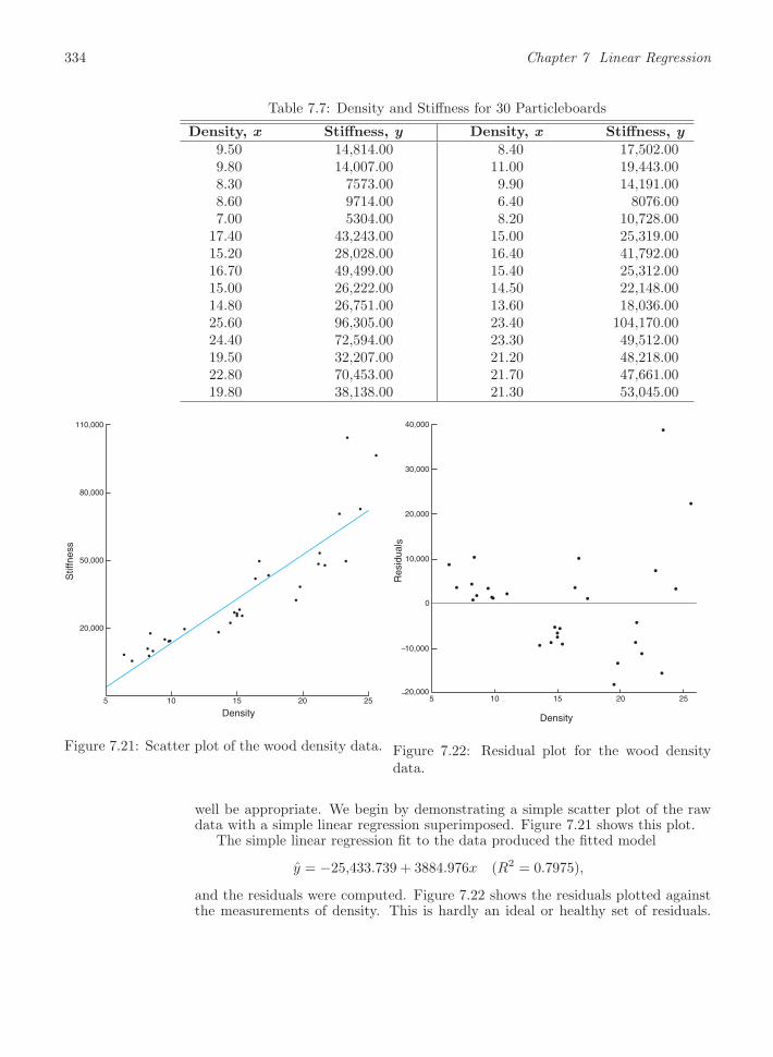
334 Chapter 7 Linear Regression
Table 7.7: Density and Stiffness for 30 Particleboards
Density, x Stiffness, y Density, x Stiffness, y9.509.808.308.607.00
17.4015.2016.7015.0014.8025.6024.4019.5022.8019.80
14,814.0014,007.007573.009714.005304.00
43,243.0028,028.0049,499.0026,222.0026,751.0096,305.0072,594.0032,207.0070,453.0038,138.00
8.4011.009.906.408.20
15.0016.4015.4014.5013.6023.4023.3021.2021.7021.30
17,502.0019,443.0014,191.008076.00
10,728.0025,319.0041,792.0025,312.0022,148.0018,036.00
104,170.0049,512.0048,218.0047,661.0053,045.00
Density
Stif
fnes
s
5 10 15 20 25
20,000
50,000
80,000
110,000
Figure 7.21: Scatter plot of the wood density data.
5 10 15 20 25−20,000
−10,000
0
10,000
20,000
30,000
40,000
Density
Res
idua
l s
Figure 7.22: Residual plot for the wood densitydata.
well be appropriate. We begin by demonstrating a simple scatter plot of the rawdata with a simple linear regression superimposed. Figure 7.21 shows this plot.
The simple linear regression fit to the data produced the fitted model
y = −25,433.739 + 3884.976x (R2 = 0.7975),
and the residuals were computed. Figure 7.22 shows the residuals plotted againstthe measurements of density. This is hardly an ideal or healthy set of residuals.

7.10 Multiple Linear Regression and Estimation of the Coefficients 335
They do not show a random scatter around a value of zero. In fact, clusters ofpositive and negative values suggest that a curvilinear trend in the data should beinvestigated.
Exercises
7.43 Compute and interpret the correlation coeffi-cient for the following grades of 6 students selected atrandom:
Mathematics grade 70 92 80 74 65 83
English grade 74 84 63 87 78 90
7.44 Use the data of Exercise 7.1 on page 303 to dothe followings.
(a) Calculate r.
(b) Test the hypothesis that ρ = 0 against the alterna-tive that ρ = 0 at the 0.05 level of significance.
7.45 With reference to Exercise 7.13 on page 306, as-sume a bivariate normal distribution for x and y.
(a) Calculate r.
(b) Test the null hypothesis that ρ = −0.5 against thealternative that ρ < −0.5 at the 0.025 level of sig-nificance.
(c) Determine the percentage of the variation in theamount of particulate removed that is due tochanges in the daily amount of rainfall.
7.46 Test the hypothesis that ρ = 0 in Exercise 7.43against the alternative that ρ = 0. Use a 0.05 level ofsignificance.
7.47 The following data were obtained in a study ofthe relationship between the weight and chest size ofinfants at birth.
Weight (kg) Chest Size (cm)2.75 29.52.15 26.34.41 32.25.52 36.53.21 27.24.32 27.72.31 28.34.30 30.33.71 28.7
(a) Calculate r.
(b) Test the null hypothesis that ρ = 0 against the al-ternative that ρ > 0 at the 0.01 level of significance.
(c) What percentage of the variation in infant chestsizes is explained by difference in weight?
7.10 Multiple Linear Regression andEstimation of the Coefficients
In most research problems where regression analysis is applied, more than oneindependent variable is needed in the regression model. The complexity of mostscientific mechanisms is such that in order to be able to predict an importantresponse, a multiple regression model is needed. When this model is linear inthe coefficients, it is called a multiple linear regression model. For the case ofk independent variables x1, x2, . . . , xk, the mean of Y |x1, x2, . . . , xk is given by themultiple linear regression model
μY |x1,x2,...,xk= β0 + β1x1 + · · ·+ βkxk,
and the estimated response is obtained from the sample regression equation
y = b0 + b1x1 + · · ·+ bkxk,
where each regression coefficient βi is estimated by bi from the sample data usingthe method of least squares. As in the case of a single independent variable, themultiple linear regression model can often be an adequate representation of a morecomplicated structure within certain ranges of the independent variables.

336 Chapter 7 Linear Regression
Similar least squares techniques can also be applied for estimating the coeffi-cients when the linear model involves, say, powers and products of the independentvariables. For example, when k = 1, the experimenter may believe that the meansμY |x do not fall on a straight line but are more appropriately described by thepolynomial regression model
μY |x = β0 + β1x+ β2x2 + · · ·+ βrx
r,
and the estimated response is obtained from the polynomial regression equation
y = b0 + b1x+ b2x2 + · · ·+ brx
r.
Confusion arises occasionally when we speak of a polynomial model as a linearmodel. However, statisticians normally refer to a linear model as one in which theparameters occur linearly, regardless of how the independent variables enter themodel. An example of a nonlinear model is the exponential relationship
μY |x = αβx,
whose response is estimated by the regression equation
y = abx.
There are many phenomena in science and engineering that are inherently non-linear in nature, and when the true structure is known, an attempt should certainlybe made to fit the actual model. The literature on estimation by least squares ofnonlinear models is voluminous. The nonlinear models discussed in this chapterdeal with nonideal conditions in which the analyst is certain that the response andhence the response model error are not normally distributed but, rather, have abinomial or Poisson distribution. These situations do occur extensively in practice.
A student who wants a more general account of nonlinear regression shouldconsult Classical and Modern Regression with Applications by Myers (1990; seethe Bibliography).
In this section, we obtain the least squares estimators of the parameters β0, β1, . . . , βk
by fitting the multiple linear regression model
μY |x1,x2,...,xk= β0 + β1x1 + · · ·+ βkxk
to the data points
{(x1i, x2i, . . . , xki, yi); i = 1, 2, . . . , n and n > k},where yi is the observed response to the values x1i, x2i, . . . , xki of the k independentvariables x1, x2, . . . , xk. Each observation (x1i, x2i, . . . , xki, yi) is assumed to satisfythe following equation.
Multiple LinearRegression Model
yi = β0 + β1x1i + β2x2i + · · ·+ βkxki + εi
or
yi = yi + ei = b0 + b1x1i + b2x2i + · · ·+ bkxki + ei,
where εi and ei are the random error and residual, respectively, associated withthe response yi and fitted value yi.

7.10 Multiple Linear Regression and Estimation of the Coefficients 337
As in the case of simple linear regression, it is assumed that the εi are independentand identically distributed with mean 0 and common variance σ2.
In using the concept of least squares to arrive at estimates b0, b1, . . . , bk, weminimize the expression
SSE =
n∑i=1
e2i =
n∑i=1
(yi − b0 − b1x1i − b2x2i − · · · − bkxki)2.
Differentiating SSE in turn with respect to b0, b1, . . . , bk and equating to zero, wegenerate the set of k + 1 normal equations for multiple linear regression.
Normal EstimationEquations for
Multiple LinearRegression
nb0 + b1
n∑i=1
x1i + b2
n∑i=1
x2i + · · · + bk
n∑i=1
xki =n∑
i=1
yi
b0
n∑i=1
x1i + b1
n∑i=1
x21i + b2
n∑i=1
x1ix2i + · · · + bk
n∑i=1
x1ixki =
n∑i=1
x1iyi
......
......
...
b0
n∑i=1
xki + b1
n∑i=1
xkix1i+ b2
n∑i=1
xkix2i + · · · + bk
n∑i=1
x2ki =
n∑i=1
xkiyi
These equations can be solved for b0, b1, b2, . . . , bk by any appropriate method forsolving systems of linear equations. Most statistical software can be used to obtainnumerical solutions of the above equations.
Example 7.10: A study was done on a diesel-powered light-duty pickup truck to see if humidity, airtemperature, and barometric pressure influence emission of nitrous oxide (in ppm).Emission measurements were taken at different times, with varying experimentalconditions. The data are given in Table 7.8. The model is
μY |x1,x2,x3= β0 + β1x1 + β2x2 + β3x3,
or, equivalently,
yi = β0 + β1x1i + β2x2i + β3x3i + εi, i = 1, 2, . . . , 20.
Fit this multiple linear regression model to the given data and then estimate theamount of nitrous oxide emitted for the conditions where humidity is 50%, tem-perature is 76◦F, and barometric pressure is 29.30.
Solution : The solution of the set of estimating equations yields the unique estimates
b0 = −3.507778, b1 = −0.002625, b2 = 0.000799, b3 = 0.154155.
Therefore, the regression equation is
y = −3.507778− 0.002625x1 + 0.000799x2 + 0.154155x3.
For 50% humidity, a temperature of 76◦F, and a barometric pressure of 29.30, theestimated amount of nitrous oxide emitted is
y = −3.507778− 0.002625(50.0) + 0.000799(76.0) + 0.1541553(29.30)
= 0.9384 ppm.

338 Chapter 7 Linear Regression
Table 7.8: Data for Example 7.10
Nitrous Humidity, Temp., Pressure, Nitrous Humidity, Temp., Pressure,Oxide, y x1 x2 x3 Oxide, y x1 x2 x3
0.900.910.960.891.001.101.151.030.771.07
72.441.634.335.110.712.98.320.172.224.0
76.370.377.168.079.067.466.876.977.767.7
29.1829.3529.2429.2729.7829.3929.6929.4829.0929.60
1.070.941.101.101.100.910.870.780.820.95
23.247.431.510.611.273.375.496.6107.454.9
76.886.676.986.386.076.377.978.786.870.9
29.3829.3529.6329.5629.4829.4029.2829.2929.0329.37
Source: Charles T. Hare, “Light-Duty Diesel Emission Correction Factors for Ambient Conditions,” EPA-600/2-77-116. U.S. Environmental Protection Agency.
Polynomial Regression
Now suppose that we wish to fit the polynomial equation
μY |x = β0 + β1x+ β2x2 + · · ·+ βrx
r
to the n pairs of observations {(xi, yi); i = 1, 2, . . . , n}. Each observation, yi,satisfies the equation
yi = β0 + β1xi + β2x2i + · · ·+ βrx
ri + εi
or
yi = yi + ei = b0 + b1xi + b2x2i + · · ·+ brx
ri + ei,
where r is the degree of the polynomial and εi and ei are again the random errorand residual associated with the response yi and fitted value yi, respectively. Here,the number of pairs, n, must be at least as large as r+1, the number of parametersto be estimated.
Notice that the polynomial model can be considered a special case of the moregeneral multiple linear regression model, where we set x1 = x, x2 = x2, . . . , xr = xr.The normal equations assume the same form as those given on page 337. They arethen solved for b0, b1, b2, . . . , br.
Example 7.11: Given the datax 0 1 2 3 4 5 6 7 8 9y 9.1 7.3 3.2 4.6 4.8 2.9 5.7 7.1 8.8 10.2
fit a regression curve of the form μY |x = β0 + β1x+ β2x2 and then estimate μY |2.
Solution : From the data given, we find that
10b0+ 45b1+ 285b2 = 63.7,
45b0+ 285b1+ 2025b2 = 307.3,
285b0+ 2025b1+ 15,333b2 = 2153.3.

7.10 Multiple Linear Regression and Estimation of the Coefficients 339
Solving these normal equations, we obtain
b0 = 8.698, b1 = −2.341, b2 = 0.288.
Therefore,
y = 8.698− 2.341x+ 0.288x2.
When x = 2, our estimate of μY |2 is
y = 8.698− (2.341)(2) + (0.288)(22) = 5.168.
Example 7.12: The data in Table 7.9 represent the percent of impurities that resulted for varioustemperatures and sterilizing times during a reaction associated with the manufac-turing of a certain beverage. Estimate the regression coefficients in the polynomialmodel
yi = β0 + β1x1i + β2x2i + β11x21i + β22x
22i + β12x1ix2i + εi,
for i = 1, 2, . . . , 18.
Table 7.9: Data for Example 7.12
Sterilizing Temperature, x1 (◦C)Time, x2 (min) 75 100 125
15
20
25
14.0514.9316.5615.8522.4121.66
10.559.4813.6311.7518.5517.98
7.556.599.238.7815.9316.44
Solution : Using the normal equations, we obtain
b0 = 56.4411, b1 = −0.36190, b2 = −2.75299,
b11 = 0.00081, b22 = 0.08173, b12 = 0.00314,
and our estimated regression equation isy = 56.4411− 0.36190x1 − 2.75299x2 + 0.00081x2
1 + 0.08173x22 + 0.00314x1x2.
Many of the principles and procedures associated with the estimation of poly-nomial regression functions fall into the category of response surface methodol-ogy, a collection of techniques that have been used quite successfully by scientistsand engineers in many fields. The x2
i are called pure quadratic terms, and thexixj (i �= j) are called interaction terms. Such problems as selecting a properexperimental design, particularly in cases where a large number of variables arein the model, and choosing optimum operating conditions for x1, x2, . . . , xk areoften approached through the use of these methods. For an extensive discussion,the reader is referred to Response Surface Methodology: Process and Product Opti-mization Using Designed Experiments by Myers, Montgomery, and Anderson-Cook(2009; see the Bibliography).

340 Chapter 7 Linear Regression
Exercises
7.48 In Applied Spectroscopy, the infrared reflectancespectra properties of a viscous liquid used in the elec-tronics industry as a lubricant were studied. The de-signed experiment consisted of testing the effect ofband frequency x1 and film thickness x2 on optical den-sity y using a Perkin-Elmer Model 621 infrared spec-trometer.
y x1 x2
0.2310.1070.0530.1290.0690.0301.0050.5590.3212.9481.6330.934
740740740805805805980980980
123512351235
1.100.620.311.100.620.311.100.620.311.100.620.31
(From Pacansky, England, and Wattman, 1986.)Estimate the multiple linear regression equation
y = b0 + b1x1 + b2x2.
7.49 A set of experimental runs was made to deter-mine a way of predicting cooking time y at variousvalues of oven width x1 and flue temperature x2. Thecoded data were recorded as follows:
y x1 x2
6.4015.0518.7530.2544.8548.9451.5561.50
100.44111.42
1.322.693.564.415.356.207.128.879.80
10.65
1.153.404.108.75
14.8215.1515.3218.1835.1940.40
Estimate the multiple linear regression equation
μY |x1,x2= β0 + β1x1 + β2x2.
7.50 An experiment was conducted to determine ifthe weight of an animal can be predicted after a givenperiod of time on the basis of the initial weight of theanimal and the amount of feed that was eaten. Use thedata, measured in kilograms, to do the followings.
(a) Fit a multiple regression equation of the form
μY |x1,x2= β0 + β1x1 + β2x2.
(b) Predict the final weight of an animal having an ini-tial weight of 35 kilograms that is given 250 kilo-grams of feed.
Final Initial FeedWeight, y Weight, x1 Weight, x2
957780
100977050809284
42333345393632414038
272226259292311183173236230235
7.51 The following data represent the chemistrygrades for a random sample of 12 freshmen at a cer-tain college along with their scores on an intelligencetest administered while they were still seniors in highschool. The number of class periods missed is alsogiven.
Chemistry Test ClassesStudent Grade, y Score, x1 Missed, x2
123456789
101112
857476908587949881917674
655055655570657055705055
175263254314
(a) Fit a multiple linear regression equation of the formy = b0 + b1x1 + b2x2.
(b) Estimate the chemistry grade for a student who hasan intelligence test score of 60 and missed 4 classes.
7.52 An experiment was conducted on a new modelof a particular make of automobile to determine thestopping distance at various speeds. The following datawere recorded.
Speed, v (km/hr) 35 50 65 80 95 110
Stopping Distance, d (m) 16 26 41 62 88 119
(a) Fit a multiple regression curve of the form μD|v =
β0 + β1v + β2v2.
(b) Estimate the stopping distance when the car istraveling at 70 kilometers per hour.
7.53 The electric power consumed each month by achemical plant is thought to be related to the averageambient temperature x1, the number of days in the

Exercises 341
month x2, the average product purity x3, and the tonsof product produced x4. The past year’s historical dataare available and are presented here.
y x1 x2 x3 x4
240236290274301316300296267276288261
253145606572808475605038
242124252526252524252523
919088879194878688919089
10095
1108894999796
11010510098
(a) Fit a multiple linear regression model using theabove data set.
(b) Predict power consumption for a month in whichx1 = 75◦F, x2 = 24 days, x3 = 90%, and x4 = 98tons.
7.54 The following is a set of coded experimental dataon the compressive strength of a particular alloy at var-ious values of the concentration of some additive:
Concentration, Compressivex Strength, y
10.015.020.025.030.0
25.229.831.231.729.4
27.331.132.630.130.8
28.727.829.732.332.8
(a) Estimate the quadratic regression equation μY |x =
β0 + β1x+ β2x2.
(b) Test for lack of fit of the model.
7.55 An experiment was conducted in order to de-termine if cerebral blood flow in human beings can bepredicted from arterial oxygen tension (millimeters ofmercury). Fifteen patients participated in the study,and the following data were collected:
Blood Flow, Arterial Oxygeny Tension, x
84.33 603.4087.80 582.5082.20 556.2078.21 594.6078.44 558.9080.01 575.2083.53 580.1079.46 451.2075.22 404.0076.58 484.0077.90 452.40
(cont.)
Blood Flow, Arterial Oxygeny Tension, x
78.80 448.4080.67 334.8086.60 320.3078.20 350.30
Estimate the quadratic regression equation
μY |x = β0 + β1x+ β2x2.
7.56 The following data are given:
x 0 1 2 3 4 5 6
y 1 4 5 3 2 3 4
(a) Fit the cubic model μY |x = β0+β1x+β2x2+β3x
3.
(b) Predict Y when x = 2.
7.57 (a) Fit a multiple regression equation of theform μY |x = β0 + β1x1 + β2x
2 to the data of Ex-ample 7.7 on page 326.
(b) Estimate the yield of the chemical reaction for atemperature of 225◦C.
7.58 The following data reflect information from 17U.S. Navy hospitals at various sites around the world.The regressors are workload variables, that is, itemsthat result in the need for personnel in a hospital. Abrief description of the variables is as follows:
y = monthly labor-hours,
x1 = average daily patient load,
x2 = monthly X-ray exposures,
x3 = monthly occupied bed-days,
x4 = eligible population in the area/1000,
x5 = average length of patient’s stay, in days.
Site x1 x2 x3 x4 x5 y
123456789
1011121314151617
15.5744.0220.4218.7449.2044.9255.4859.2894.39
128.0296.00
131.42127.21252.90409.20463.70510.22
24632048394065055723
11,520577959698461
20,10613,31310,77115,54336,19434,70339,20486,533
472.921339.75620.25568.33
1497.601365.831687.001639.922872.333655.082912.003921.003865.677684.10
12,446.3314,098.4015,524.00
18.09.5
12.836.735.724.043.346.778.7
180.560.9
103.7126.8157.7169.4331.4371.6
4.456.924.283.905.504.605.625.156.186.155.884.885.507.00
10.757.056.35
566.52696.82
1033.151003.621611.371613.271854.172160.552305.583503.933571.593741.404026.52
10,343.8111,732.1715,414.9418,854.45
The goal here is to produce an empirical equation thatwill estimate (or predict) personnel needs for naval hos-

342 Chapter 7 Linear Regression
pitals. Estimate the multiple linear regression equation
μY |x1,x2,x3,x4,x5
= β0 + β1x1 + β2x2 + β3x3 + β4x4 + β5x5.
7.59 An experiment was conducted to study the sizeof squid eaten by sharks and tuna. The regressor vari-ables are characteristics of the beaks of the squid. Thedata are given as follows:
x1 x2 x3 x4 x5 y
1.311.550.990.991.011.091.081.270.991.341.301.331.861.581.971.801.751.721.681.752.191.73
1.071.490.840.830.900.930.901.080.851.131.101.101.471.341.591.561.581.431.571.591.861.67
0.440.530.340.340.360.420.400.440.360.450.450.480.600.520.670.660.630.640.720.680.750.64
0.750.900.570.540.640.610.510.770.560.770.760.771.010.951.201.021.091.020.961.081.241.14
0.350.470.320.270.300.310.310.340.290.370.380.380.650.500.590.590.590.630.680.620.720.55
1.952.900.720.811.091.221.021.930.642.081.981.908.564.498.496.177.546.367.637.78
10.156.88
In the study, the regressor variables and response con-sidered are
x1 = rostral length, in inches,
x2 = wing length, in inches,
x3 = rostral to notch length, in inches,
x4 = notch to wing length, in inches,
x5 = width, in inches,
y = weight, in pounds.
Estimate the multiple linear regression equation
μY |x1,x2,x3,x4,x5
= β0 + β1x1 + β2x2 + β3x3 + β4x4 + β5x5.
7.60 An engineer at a semiconductor company wantsto model the relationship between the gain or hFE ofa device (y) and three parameters: emitter-RS (x1),base-RS (x2), and emitter-to-base-RS (x3). The dataare presented here are from Myers, Montgomery, andAnderson-Cook, 2009.
(a) Fit a multiple linear regression to the data.
(b) Predict hFE when x1 = 14, x2 = 220, and x3 = 5.
x1, x2, x3, y,Emitter-RS Base-RS E-B-RS hFE
14.6215.6314.6215.0014.5015.2516.1215.1315.5015.1315.5016.1215.1315.6315.3815.50
226.0220.0217.4220.0226.5224.1220.5223.5217.6228.5230.2226.5226.6225.6234.0230.0
7.0003.3756.3756.0007.6256.0003.3756.1255.0006.6255.7503.7506.1255.3758.8754.000
128.4052.62
113.9098.01
139.90102.6048.14
109.6082.68
112.6097.5259.06
111.8089.09
171.9066.80
7.61 A study was performed on a type of bearingto find the relationship of amount of wear y to x1 =oil viscosity and x2 = load. The following data wereobtained.
y x1 x2 y x1 x2
193172113
1.622.033.0
85110581357
23091
125
15.543.040.0
81612011115
(Data from Myers, Montgomery, and Anderson-Cook,2009.)
(a) Estimate the unknown parameters of the multiplelinear regression equation
μY |x1,x2= β0 + β1x1 + β2x2.
(b) Predict wear when oil viscosity is 20 and load is1200.
7.62 Eleven student teachers took part in an evalu-ation program designed to measure teacher effective-ness and determine what factors are important. Theresponse measure was a quantitative evaluation of theteacher. The regressor variables were scores on fourstandardized tests given to each teacher. The data areas follows:
y x1 x2 x3 x4
410569425344324505235501400584434
695777810
537776659776
125131141122141152141132157166141
59.0031.7580.5075.0049.0049.3560.7541.2550.7532.2554.50
55.6663.9745.3246.6741.2143.8341.6164.5742.4157.9557.90

7.11 Inferences in Multiple Linear Regression 343
Estimate the multiple linear regression equation
μY |x1,x2,x3,x4= β0 + β1x1 + β2x2 + β3x3 + β4x4.
7.63 The personnel department of a certain industrialfirm used 12 subjects in a study to determine the rela-tionship between job performance rating (y) and scoreson four tests. Use the data provided here to estimatethe regression coefficients in the model
y = b0 + b1x1 + b2x2 + b3x3 + b4x4.
y x1 x2 x3 x4
11.2 56.5 71.0 38.5 43.014.5 59.5 72.5 38.2 44.817.2 69.2 76.0 42.5 49.017.8 74.5 79.5 43.4 56.319.3 81.2 84.0 47.5 60.224.5 88.0 86.2 47.4 62.021.2 78.2 80.5 44.5 58.116.9 69.0 72.0 41.8 48.114.8 58.1 68.0 42.1 46.020.0 80.5 85.0 48.1 60.313.2 58.3 71.0 37.5 47.122.5 84.0 87.2 51.0 65.2
7.11 Inferences in Multiple Linear Regression
The means and variances of the estimators b0, b1, . . . , bk are readily obtained undercertain assumptions on the random errors ε1, ε2, . . . , εk that are identical to thosemade in the case of simple linear regression. When we assume these errors to beindependent, each with mean 0 and variance σ2, it can be shown that b0, b1, . . . , bkare, respectively, unbiased estimators of the regression coefficients β0, β1, . . . , βk.In addition, the variances of the b’s are obtained through the elements of the inverseof the A matrix. Note that the off-diagonal elements of A = X′X represent sumsof products of elements in the columns of X, while the diagonal elements of Arepresent sums of squares of elements in the columns of X. The inverse matrix,A−1, apart from the multiplier σ2, represents the variance-covariance matrixof the estimated regression coefficients. That is, the elements of the matrix A−1σ2
display the variances of b0, b1, . . . , bk on the main diagonal and covariances on theoff-diagonal. For example, in a k = 2 multiple linear regression problem, we mightwrite
(X′X)−1 =
⎡⎣c00 c01 c02c10 c11 c12c20 c21 c22
⎤⎦with the elements below the main diagonal determined through the symmetry ofthe matrix. Then we can write
σ2bi = ciiσ
2, i = 0, 1, 2,
σbibj = Cov(bi, bj)= cijσ2, i �= j.
Of course, the estimates of the variances and hence the standard errors of theseestimators are obtained by replacing σ2 with the appropriate estimate obtainedthrough experimental data. An unbiased estimate of σ2 is once again defined interms of the error sum of squares, which is computed using the formula establishedin Theorem 7.2. In the theorem, we are making the assumptions on the εi describedabove.

344 Chapter 7 Linear Regression
Theorem 7.2: For the linear regression equation
y = Xβ + ε,
an unbiased estimate of σ2 is given by the error or residual mean square
s2 =SSE
n− k − 1, where SSE =
n∑i=1
e2i =n∑
i=1
(yi − yi)2.
We can see that Theorem 7.2 represents a generalization of Theorem 7.1 for thesimple linear regression case. The proof is left for the reader. As in the simplerlinear regression case, the estimate s2 is a measure of the variation in the predictionerrors or residuals.
The error and regression sums of squares take on the same form and play thesame role as in the simple linear regression case. In fact, the sum-of-squares identity
n∑i=1
(yi − y)2 =
n∑i=1
(yi − y)2 +
n∑i=1
(yi − yi)2
continues to hold, and we retain our previous notation, namely
SST = SSR+ SSE,
with
SST =
n∑i=1
(yi − y)2 = total sum of squares
and
SSR =n∑
i=1
(yi − y)2 = regression sum of squares.
There are k degrees of freedom associated with SSR, and, as always, SST hasn− 1 degrees of freedom. Therefore, after subtraction, SSE has n− k− 1 degreesof freedom. Thus, our estimate of σ2 is again given by the error sum of squaresdivided by its degrees of freedom. All three of these sums of squares will appearon the printouts of most multiple regression computer packages. Note that thecondition n > k in Section 7.10 guarantees that the degrees of freedom of SSEcannot be negative.
Analysis of Variance in Multiple Regression
The partition of the total sum of squares into its components, the regression anderror sums of squares, plays an important role. An analysis of variance canbe conducted to shed light on the quality of the regression equation. A usefulhypothesis that determines if a significant amount of variation is explained by themodel is
H0: β1 = β2 = β3 = · · · = βk = 0.

7.11 Inferences in Multiple Linear Regression 345
The analysis of variance involves an F -test which can be summarized via a tableas follows:
Source Sum of Squares Degrees of Freedom Mean Squares F
Regression SSR k MSR = SSRk f = MSR
MSE
Error SSE n− (k + 1) MSE = SSEn−(k+1)
Total SST n− 1
This test is an upper-tailed test. Rejection of H0 implies that the regressionequation differs from a constant. That is, at least one regressor variable isimportant. However, this and other tests of hypotheses considered later requirethat the errors εi be normally distributed in the multiple linear regression model.
Further utility of the mean square error (or residual mean square) lies in itsuse in hypothesis testing and confidence interval estimation. In addition, the meansquare error plays an important role in situations where the scientist is searchingfor the best from a set of competing models. Many model-building criteria involvethe statistic s2.
A knowledge of the distributions of the individual coefficient estimators enablesthe experimenter to construct confidence intervals for the coefficients and to testhypotheses about them. Since the bj (j = 0, 1, 2, . . . , k) are normally distributedwith mean βj and variance cjjσ
2, we can use the statistic
t =bj − βj0
s√cjj
with n − k − 1 degrees of freedom to test hypotheses and construct confidenceintervals on βj . For example, if we wish to test
H0: βj = βj0,
H1: βj �= βj0,
we compute the above t-statistic and do not reject H0 if −tα/2 < t < tα/2, wheretα/2 has n− k − 1 degrees of freedom.
Individual t-Tests for Variable Screening
The t-test most often used in multiple regression is the one that tests the impor-tance of individual coefficients (i.e., H0: βj = 0 against the alternative H1: βj �= 0).These tests often contribute to what is termed variable screening, where the ana-lyst attempts to arrive at the most useful model (i.e., the choice of which regressorsto use). It should be emphasized here that if a coefficient is found insignificant (i.e.,the hypothesis H0: βj = 0 is not rejected), the conclusion drawn is that the vari-able is insignificant (i.e., explains an insignificant amount of variation in y), in thepresence of the other regressors in the model.

346 Chapter 7 Linear Regression
Exercises
7.64 For the data of Exercise 7.49 on page 340, esti-mate σ2.
7.65 For the data of Exercise 7.48 on page 340, esti-mate σ2.
7.66 Obtain estimates of the variances and the co-variance of the estimators b1 and b2 of Exercise 7.48on page 340.
7.67 For the data of Exercise 7.53 on page 340, esti-mate σ2.
7.68 For the model of Exercise 7.55 on page 341, testthe hypothesis that β2 = 0 at the 0.05 level of signifi-cance against the alternative that β2 = 0.
7.69 Referring to Exercise 7.53 on page 340, find theestimate of
(a) σ2b2;
(b) Cov(b1, b4).
7.70 For the model of Exercise 7.49 on page 340, testthe hypothesis that β1 = 2 against the alternative thatβ1 = 2. Use a P-value in your conclusion.
7.71 For the model of Exercise 7.48 on page 340, testthe hypothesis that β1 = 0 at the 0.05 level of signifi-cance against the alternative that β1 = 0.
7.72 For Exercise 7.54 on page 341, construct a 90%confidence interval for the mean compressive strengthwhen the concentration is x = 19.5 and a quadraticmodel is used.
7.73 Using the data of Exercise 7.48 on page 340 andthe estimate of σ2 from Exercise 7.65, compute 95%confidence intervals for the predicted response and themean response when x1 = 900 and x2 = 1.00.
7.74 Consider the following data from Exercise 7.61on page 342.
y (wear) x1 (oil viscosity) x2 (load)193 1.6 851230 15.5 816172 22.0 105891 43.0 1201113 33.0 1357125 40.0 1115
(a) Estimate σ2 using multiple regression of y on x1
and x2.
(b) Compute predicted values, a 95% confidence inter-val for mean wear, and a 95% prediction intervalfor observed wear if x1 = 20 and x2 = 1000.
7.75 Using the data of Exercise 7.53 on page 340 andthe estimate of σ2 from Exercise 7.67, compute 95%confidence intervals for the predicted response and themean response when x1 = 75, x2 = 24, x3 = 90, andx4 = 98.
7.76 Use the data from Exercise 7.60 on page 342.
(a) Estimate σ2 using the multiple regression of y onx1, x2, and x3.
(b) Compute a 95% prediction interval for the ob-served gain with the three regressors at x1 = 15.0,x2 = 220.0, and x3 = 6.0.
7.77 Using the data from Exercise 7.74, test the fol-lowing at the 0.05 level.
(a) H0: β1 = 0 versus H1: β1 = 0;
(b) H0: β2 = 0 versus H1: β2 = 0.
(c) Do you have any reason to believe that the modelin Exercise 7.74 should be changed? Why or whynot?
Review Exercises
7.78 With reference to Exercise 7.8 on page 305, con-struct
(a) a 95% confidence interval for the average coursegrade of students who score 35 on the placementtest;
(b) a 95% prediction interval for the course grade of astudent who scored 35 on the placement test.
7.79 The Statistics Consulting Center at VirginiaTech analyzed data on normal woodchucks for the De-
partment of Veterinary Medicine. The variables of in-terest were body weight in grams and heart weight ingrams. It was desired to develop a linear regressionequation in order to determine if there is a signifi-cant linear relationship between heart weight and totalbody weight. Use heart weight as the independent vari-able and body weight as the dependent variable andfit a simple linear regression using the following data.In addition, test the hypothesis H0 : β1 = 0 versusH1: β1 = 0. Draw conclusions.

Review Exercises 347
Body Weight (grams) Heart Weight (grams)4050246531205700259536402050423529354975369028002775217023702055202526452675
11.212.410.513.29.8
11.010.810.412.211.210.814.212.210.012.312.511.816.013.8
7.80 The amounts of solids removed from a particu-lar material when exposed to drying periods of differentlengths are as shown.
x (hours) y (grams)4.4 13.1 14.24.5 9.0 11.54.8 10.4 11.55.5 13.8 14.85.7 12.7 15.15.9 9.9 12.76.3 13.8 16.56.9 16.4 15.77.5 17.6 16.97.8 18.3 17.2
(a) Estimate the linear regression line.
(b) Test at the 0.05 level of significance whether thelinear model is adequate.
7.81 With reference to Exercise 7.9 on page 305, con-struct
(a) a 95% confidence interval for the average weeklysales when $45 is spent on advertising;
(b) a 95% prediction interval for the weekly sales when$45 is spent on advertising.
7.82 An experiment was designed for the Departmentof Materials Engineering at Virginia Tech to study hy-drogen embrittlement properties based on electrolytichydrogen pressure measurements. The solution usedwas 0.1 N NaOH, and the material was a certain typeof stainless steel. The cathodic charging current den-sity was controlled and varied at four levels. The effec-tive hydrogen pressure was observed as the response.The data follow.
Charging Current EffectiveDensity, x Hydrogen
Run ( mA/cm2) Pressure, y (atm)123456789
101112131415
0.50.50.50.51.51.51.52.52.52.52.53.53.53.53.5
86.192.164.774.7
223.6202.1132.9413.5231.5466.7365.3493.7382.3447.2563.8
(a) Run a simple linear regression of y against x.
(b) Compute the pure error sum of squares and makea test for lack of fit.
(c) Does the information in part (b) indicate a needfor a model in x beyond a first-order regression?Explain.
7.83 The following data represent the chemistrygrades for a random sample of 12 freshmen at a cer-tain college along with their scores on an intelligencetest administered while they were still seniors in highschool.
Test ChemistryStudent Score, x Grade, y
123456789
101112
655055655570657055705055
857476908587949881917674
(a) Compute and interpret the sample correlation co-efficient.
(b) State necessary assumptions on random variables.
(c) Test the hypothesis that ρ = 0.5 against the alter-native that ρ > 0.5. Use a P-value in the conclu-sion.
7.84 The Washington Times business section inMarch of 1997 listed 21 different used computers andprinters and their sale prices. Also listed was the aver-age hover bid. Partial results from regression analysis

348 Chapter 7 Linear Regression
using SAS software are shown in Figure 7.23 on page350.
(a) Explain the difference between the confidence in-terval on the mean and the prediction interval.
(b) Explain why the standard errors of prediction varyfrom observation to observation.
(c) Which observation has the lowest standard error ofprediction? Why?
7.85 Consider the vehicle data from Consumer Re-ports in Figure 7.24 on page 351. The data includeweight (in tons), mileage (in miles per gallon), anddrive ratio. A regression model was fitted relatingweight x to mileage y. A partial SAS printout in Fig-ure 7.24 shows some of the results of that regressionanalysis, and Figure 7.25 on page 352 gives a plot ofthe residuals and weight for each vehicle.
(a) From the analysis and the residual plot, does it ap-pear that an improved model might be found byusing a transformation? Explain.
(b) Fit the model by replacing weight with log weight.Comment on the results.
(c) Fit a model by replacing mpg with gallons per 100miles traveled, as mileage is often reported in othercountries. Which of the three models is preferable?Explain.
7.86 Observations on the yield of a chemical reactiontaken at various temperatures were recorded as follows:
x (◦C) y (%) x (◦C) y (%)150 75.4 150 77.7150 81.2 200 84.4200 85.5 200 85.7250 89.0 250 89.4250 90.5 300 94.8300 96.7 300 95.3
(a) Plot the data.
(b) Does it appear from the plot as if the relationshipis linear?
(c) Fit a simple linear regression and test for lack offit.
(d) Draw conclusions based on your result in (c).
7.87 Physical fitness testing is an important aspectof athletic training. A common measure of the mag-nitude of cardiovascular fitness is the maximum vol-ume of oxygen uptake during strenuous exercise. Astudy was conducted on 24 middle-aged men to de-termine the influence on oxygen uptake of the timerequired to complete a two-mile run. Oxygen uptakewas measured with standard laboratory methods as thesubjects performed on a treadmill. The work was pub-lished in “Maximal Oxygen Intake Prediction in Youngand Middle Aged Males,” Journal of Sports Medicine
9, 1969, 17–22. The data are as follows:
y, Maximum x, TimeSubject Volume of O2 in Seconds
123456789
101112131415161718192021222324
42.3353.1042.0850.0642.4542.4647.8249.9236.2349.6641.4946.1746.1843.2151.8153.2853.2947.1856.9147.8048.6553.6760.6256.73
918805892962968907770743
1045810927813858860760747743803683844755700748775
(a) Estimate the parameters in a simple linear regres-sion model.
(b) Does the time it takes to run two miles have a sig-nificant influence on maximum oxygen uptake? UseH0: β1 = 0 versus H1: β1 = 0.
(c) Plot the residuals on a graph against x and com-ment on the appropriateness of the simple linearmodel.
7.88 Consider the fictitious set of data shown below,where the line through the data is the fitted simplelinear regression line. Sketch a residual plot.
x
y

Review Exercises 349
7.89 Consider a 2nd-order response surface modelthat contains the linear, pure quadratic and cross-product terms as follows:
yi = β0 + β1x1i + β2x2i + β11x21i
+ β22x22i + β12x1ix2i + εi.
Fit the model above to the following data, and suggestany model editing that may be needed.
x1 x2 y
−1−1−1000111
−101
−101
−101
35.3838.4242.1536.5245.2753.2237.1848.2555.07
7.90 A study was conducted to determine whetherlifestyle changes could replace medication in reducingblood pressure among hypertensives. The factors con-sidered were a healthy diet with an exercise program,the typical dosage of medication for hypertension, andno intervention. The pretreatment body mass index(BMI) was also calculated because it is known to affectblood pressure. The response considered in this studywas change in blood pressure. The variable “group”had the following levels.
1 = Healthy diet and an exercise program
2 = Medication
3 = No intervention
(a) Fit an appropriate model using the data below.Does it appear that exercise and diet could be effec-tively used to lower blood pressure? Explain youranswer from the results.
(b) Would exercise and diet be an effective alternativeto medication?
(Hint: You may wish to form the model in more thanone way to answer both of these questions.)
Change inBlood Pressure Group BMI
−32−21−26−16−11−19−23−5−65
−1114
111122223333
27.322.126.127.819.226.128.623.028.125.326.722.3
7.91 Show that in choosing the so-called best subsetmodel from a series of candidate models, choosing themodel with the smallest s2 is equivalent to choosingthe model with the smallest R2
adj.
7.92 Case Study: Consider the data set for Exercise7.58, page 341 (hospital data), repeated here.
Site x1 x2 x3 x4 x5 y
123456789
1011121314151617
15.5744.0220.4218.7449.2044.9255.4859.2894.39
128.0296.00
131.42127.21252.90409.20463.70510.22
24632048394065055723
11,520577959698461
20,10613,31310,77115,54336,19434,70339,20486,533
472.921339.75620.25568.33
1497.601365.831687.001639.922872.333655.082912.003921.003865.677684.10
12,446.3314,098.4015,524.00
18.09.5
12.836.735.724.043.346.778.7
180.560.9
103.7126.8157.7169.4331.4371.6
4.456.924.283.905.504.605.625.l56.186.155.884.885.507.00
10.757.056.35
566.52696.82
1033.151003.621611.371613.271854.172160.552305.583503.933571.593741.404026.52
10,343.8111,732.1715,414.9418,854.45
(a) The SAS PROC REG outputs provided in Figures7.26 and 7.27 on pages 353 and 354 supply a con-siderable amount of information. Goals are to dooutlier detection and eventually determine whichmodel terms are to be used in the final model.
(b) Often the role of a single regressor variable is notapparent when it is studied in the presence of sev-eral other variables. This is due to multicollinear-ity. With this in mind, comment on the importanceof x2 and x3 in the full model as opposed to theirimportance in a model in which they are the onlyvariables.
(c) Comment on what other analyses should be run.
(d) Run appropriate analyses and write your conclu-sions concerning the final model.
7.93 Project: This project can be done in groups orby individuals. Each person or group must find a set ofdata, preferably from (but not restricted to) their fieldof study. The data need to fit the regression frameworkwith a regression variable x and a response variable y.Carefully make the assignment as to which variable is xand which y. It may be necessary to consult a journalor periodical from your field if you do not have otherresearch data available.
(a) Plot y versus x. Comment on the relationship asseen from the plot.
(b) Fit an appropriate regression model from the data.Use simple linear regression or fit a polynomial

350 Chapter 7 Linear Regression
model to the data. Comment on measures of qual-ity.
(c) Plot residuals as illustrated in the text. Check pos-
sible violation of assumptions. Show graphicallya plot of confidence intervals on a mean responseplotted against x. Comment.
R-Square Coeff Var Root MSE Price Mean0.967472 7.923338 70.83841 894.0476
StandardParameter Estimate Error t Value Pr > |t|Intercept 59.93749137 38.34195754 1.56 0.1345Buyer 1.04731316 0.04405635 23.77 <.0001
Predict Std Err Lower 95% Upper 95% Lower 95% Upper 95%product Buyer Price Value Predict Mean Mean Predict PredictIBM PS/1 486/66 420MB 325 375 400.31 25.8906 346.12 454.50 242.46 558.17IBM ThinkPad 500 450 625 531.23 21.7232 485.76 576.70 376.15 686.31IBM Think-Dad 755CX 1700 1850 1840.37 42.7041 1750.99 1929.75 1667.25 2013.49AST Pentium 90 540MB 800 875 897.79 15.4590 865.43 930.14 746.03 1049.54Dell Pentium 75 1GB 650 700 740.69 16.7503 705.63 775.75 588.34 893.05Gateway 486/75 320MB 700 750 793.06 16.0314 759.50 826.61 641.04 945.07Clone 586/133 1GB 500 600 583.59 20.2363 541.24 625.95 429.40 737.79Compaq Contura 4/25 120MB 450 600 531.23 21.7232 485.76 576.70 376.15 686.31Compaq Deskpro P90 1.2GB 800 850 897.79 15.4590 865.43 930.14 746.03 1049.54Micron P75 810MB 800 675 897.79 15.4590 865.43 930.14 746.03 1049.54Micron P100 1.2GB 900 975 1002.52 16.1176 968.78 1036.25 850.46 1154.58Mac Quadra 840AV 500MB 450 575 531.23 21.7232 485.76 576.70 376.15 686.31Mac Performer 6116 700MB 700 775 793.06 16.0314 759.50 826.61 641.04 945.07PowerBook 540c 320MB 1400 1500 1526.18 30.7579 1461.80 1590.55 1364.54 1687.82PowerBook 5300 500MB 1350 1575 1473.81 28.8747 1413.37 1534.25 1313.70 1633.92Power Mac 7500/100 1GB 1150 1325 1264.35 21.9454 1218.42 1310.28 1109.13 1419.57NEC Versa 486 340MB 800 900 897.79 15.4590 865.43 930.14 746.03 1049.54Toshiba 1960CS 320MB 700 825 793.06 16.0314 759.50 826.61 641.04 945.07Toshiba 4800VCT 500MB 1000 1150 1107.25 17.8715 1069.85 1144.66 954.34 1260.16HP Laser jet III 350 475 426.50 25.0157 374.14 478.86 269.26 583.74Apple Laser Writer Pro 63 750 800 845.42 15.5930 812.79 878.06 693.61 997.24
Figure 7.23: SAS printout, showing partial analysis of data of Review Exercise 7.84.

Review Exercises 351
Obs Model WT MPG DR_RATIO1 Buick Estate Wagon 4.360 16.9 2.732 Ford Country Squire Wagon 4.054 15.5 2.263 Chevy Ma libu Wagon 3.605 19.2 2.564 Chrysler LeBaron Wagon 3.940 18.5 2.455 Chevette 2.155 30.0 3.706 Toyota Corona 2.560 27.5 3.057 Datsun 510 2.300 27.2 3.548 Dodge Omni 2.230 30.9 3.379 Audi 5000 2.830 20.3 3.90
10 Volvo 240 CL 3.140 17.0 3.5011 Saab 99 GLE 2.795 21.6 3.7712 Peugeot 694 SL 3.410 16.2 3.5813 Buick Century Special 3.380 20.6 2.7314 Mercury Zephyr 3.070 20.8 3.0815 Dodge Aspen 3.620 18.6 2.7116 AMC Concord D/L 3.410 18.1 2.7317 Chevy Caprice Classic 3.840 17.0 2.4118 Ford LTP 3.725 17.6 2.2619 Mercury Grand Marquis 3.955 16.5 2.2620 Dodge St Regis 3.830 18.2 2.4521 Ford Mustang 4 2.585 26.5 3.0822 Ford Mustang Ghia 2.910 21.9 3.0823 Macda GLC 1.975 34.1 3.7324 Dodge Colt 1.915 35.1 2.9725 AMC Spirit 2.670 27.4 3.0826 VW Scirocco 1.990 31.5 3.7827 Honda Accord LX 2.135 29.5 3.0528 Buick Skylark 2.570 28.4 2.5329 Chevy Citation 2.595 28.8 2.6930 Olds Omega 2.700 26.8 2.8431 Pontiac Phoenix 2.556 33.5 2.6932 Plymouth Horizon 2.200 34.2 3.3733 Datsun 210 2.020 31.8 3.7034 Fiat Strada 2.130 37.3 3.1035 VW Dasher 2.190 30.5 3.7036 Datsun 810 2.815 22.0 3.7037 BMW 320i 2.600 21.5 3.6438 VW Rabbit 1.925 31.9 3.78
R-Square Coeff Var Root MSE MPG Mean0.817244 11.46010 2.837580 24.76053
StandardParameter Estimate Error t Value Pr > |t|Intercept 48.67928080 1.94053995 25.09 <.0001WT -8.36243141 0.65908398 -12.69 <.0001
Figure 7.24: SAS printout, showing partial analysis of data of Review Exercise 7.85.

352 Chapter 7 Linear Regression
Plot of Resid*WT. Symbol used is ’*’.
Resid |8 +
||||| * *
6 +|||| *|
4 + *|||| *| *
2 + *| * *| *| * * *| * * *| * * * *
0 +-----------------*---*------------------------------------------*------------------------|| * * * *|| *|
-2 + *| * * *|| *|| *
-4 + *|| *|| * *|
-6 +|---+-------------+-------------+-------------+-------------+-------------+-------------+--1.5 2.0 2.5 3.0 3.5 4.0 4.5
WT
Figure 7.25: SAS printout, showing residual plot of Review Exercise 7.85.

Review Exercises 353
Dependent Variable: yAnalysis of Variance
Sum of MeanSource DF Squares Square F Value Pr > FModel 5 490177488 98035498 237.79 <.0001Error 11 4535052 412277Corrected Total 16 494712540
Root MSE 642.08838 R-Square 0.9908Dependent Mean 4978.48000 Adj R-Sq 0.9867Coeff Var 12.89728
Parameter EstimatesParameter Standard
Variable Label DF Estimate Error t Value Pr > |t|Intercept Intercept 1 1962.94816 1071.36170 1.83 0.0941x1 Average Daily Patient Load 1 -15.85167 97.65299 -0.16 0.8740x2 Monthly X-Ray Exposure 1 0.05593 0.02126 2.63 0.0234x3 Monthly Occupied Bed Days 1 1.58962 3.09208 0.51 0.6174x4 Eligible Population in the 1 -4.21867 7.17656 -0.59 0.5685
Area/100x5 Average Length of Patients 1 -394.31412 209.63954 -1.88 0.0867
Stay in Days
Figure 7.26: SAS output for Review Exercise 7.92; part I.

354 Chapter 7 Linear Regression
Dependent Predicted Std ErrorObs Variable Value Mean Predict 95% CL Mean 95% CL Predict1 566.5200 775.0251 241.2323 244.0765 1306 -734.6494 22852 696.8200 740.6702 331.1402 11.8355 1470 -849.4275 23313 1033 1104 278.5116 490.9234 1717 -436.5244 26444 1604 1240 268.1298 650.3459 1831 -291.0028 27725 1611 1564 211.2372 1099 2029 76.6816 30526 1613 2151 279.9293 1535 2767 609.5796 36937 1854 1690 218.9976 1208 2172 196.5345 31838 2161 1736 468.9903 703.9948 2768 -13.8306 34869 2306 2737 290.4749 2098 3376 1186 428810 3504 3682 585.2517 2394 4970 1770 559411 3572 3239 189.0989 2823 3655 1766 471312 3741 4353 328.8507 3630 5077 2766 594113 4027 4257 314.0481 3566 4948 2684 583014 10344 8768 252.2617 8213 9323 7249 1028615 11732 12237 573.9168 10974 13500 10342 1413316 15415 15038 585.7046 13749 16328 13126 1695117 18854 19321 599.9780 18000 20641 17387 21255
Std Error StudentObs Residual Residual Residual -2-1 0 1 21 -208.5051 595.0 -0.350 | | |2 -43.8502 550.1 -0.0797 | | |3 -70.7734 578.5 -0.122 | | |4 363.1244 583.4 0.622 | |* |5 46.9483 606.3 0.0774 | | |6 -538.0017 577.9 -0.931 | *| |7 164.4696 603.6 0.272 | | |8 424.3145 438.5 0.968 | |* |9 -431.4090 572.6 -0.753 | *| |10 -177.9234 264.1 -0.674 | *| |11 332.6011 613.6 0.542 | |* |12 -611.9330 551.5 -1.110 | **| |13 -230.5684 560.0 -0.412 | | |14 1576 590.5 2.669 | |***** |15 -504.8574 287.9 -1.753 | ***| |16 376.5491 263.1 1.431 | |** |17 -466.2470 228.7 -2.039 | ****| |
Figure 7.27: SAS output for Review Exercise 7.92; part II.

Chapter 8
One-Factor Experiments: General
8.1 Analysis-of-Variance Technique and the Strategy ofExperimental Design
In the estimation and hypothesis testing material covered in Chapters 5 and 6, wewere restricted in each case to considering no more than two population parameters.Such was the case, for example, in testing for the equality of two population meansusing independent samples from normal populations with common but unknownvariance, where it was necessary to obtain a pooled estimate of σ2. This materialdealing in two-sample inference represents a special case of what we call the one-factor problem. For example, in Exercise 6.35 on page 269, the survival time wasmeasured for two samples of mice, where one sample received a new serum forleukemia treatment and the other sample received no treatment. In this case, wesay that there is one factor, namely treatment, and the factor is at two levels.If several competing treatments were being used in the sampling process, moresamples of mice would be necessary. In this case, the problem would involve onefactor with more than two levels and thus more than two samples.
In the k > 2 sample problem, it will be assumed that there are k samples fromk populations. One very common procedure used to deal with testing populationmeans is called the analysis of variance, or ANOVA.
The analysis of variance is certainly not a new technique to the reader whohas followed the material on regression theory. We used the analysis-of-varianceapproach to partition the total sum of squares into a portion due to regression anda portion due to error.
Suppose in an industrial experiment that an engineer is interested in how themean absorption of moisture in concrete varies among 5 different concrete aggre-gates. The samples are exposed to moisture for 48 hours. It is decided that 6samples are to be tested for each aggregate, requiring a total of 30 samples to betested. The data are recorded in Table 8.1.
The model for this situation may be set up as follows. There are 6 observationstaken from each of 5 populations with means μ1, μ2, . . . , μ5, respectively. We may
355

356 Chapter 8 One-Factor Experiments
Table 8.1: Absorption of Moisture in Concrete Aggregates
Aggregate: 1 2 3 4 5
551 595 639 417 563457 580 615 449 631450 508 511 517 522731 583 573 438 613499 633 648 415 656632 517 677 555 679
Total 3320 3416 3663 2791 3664 16,854Mean 553.33 569.33 610.50 465.17 610.67 561.80
wish to test
H0: μ1 = μ2 = · · · = μ5,
H1: At least two of the means are not equal.
In addition, we may be interested in making individual comparisons among these5 population means.
In the analysis-of-variance procedure, it is assumed that whatever variation ex-ists among the aggregate averages is attributed to (1) variation in absorption amongobservations within aggregate types and (2) variation among aggregate types, thatis, due to differences in the chemical composition of the aggregates. The within-aggregate variation is, of course, brought about by various causes. Perhapshumidity and temperature conditions were not kept entirely constant throughoutthe experiment. It is possible that there was a certain amount of heterogeneity inthe batches of raw materials that were used. At any rate, we shall consider thewithin-sample variation to be chance or random variation. Part of the goal ofthe analysis of variance is to determine if the differences among the 5 sample meansare what we would expect due to random variation alone or, rather, due to varia-tion beyond merely random effects, i.e., differences in the chemical composition ofthe aggregates.
Many pointed questions appear at this stage concerning the preceding problem.For example, how many samples must be tested for each aggregate? This is aquestion that continually haunts the practitioner. In addition, what if the within-sample variation is so large that it is difficult for a statistical procedure to detectthe systematic differences? Can we systematically control extraneous sources ofvariation and thus remove them from the portion we call random variation? Weshall attempt to answer these and other questions in the following sections.
In Chapters 5 and 6, the notions of estimation and testing for the two-samplecase were covered against the important backdrop of the way the experiment isconducted. This discussion falls into the broad category of design of experiments.For example, for the pooled t-test discussed in Chapter 6, it is assumed that thefactor levels (treatments in the mice example) are assigned randomly to the exper-imental units (mice). The notion of experimental units was discussed in Chapters5 and 6 and illustrated through examples. Simply put, experimental units are the

8.2 One-Way Analysis of Variance: Completely Randomized Design 357
units (mice, patients, concrete specimens, time) that provide the heterogene-ity that leads to experimental error in a scientific investigation. The randomassignment eliminates bias that could result with systematic assignment. The goalis to distribute uniformly among the factor levels the risks brought about by theheterogeneity of the experimental units. Random assignment best simulates theconditions that are assumed by the model. In Section 8.5, we discuss blockingin experiments. The notion of blocking was presented in Chapters 5 and 6, whencomparisons between means were accomplished with pairing, that is, the divisionof the experimental units into homogeneous pairs called blocks. The factor levelsor treatments are then assigned randomly within blocks. The purpose of blocking isto reduce the effective experimental error. In this chapter, we naturally extend thepairing to larger block sizes, with analysis of variance being the primary analyticaltool.
8.2 One-Way Analysis of Variance (One-Way ANOVA):Completely Randomized Design
Random samples of size n are selected from each of k populations. The k differ-ent populations are classified on the basis of a single criterion such as differenttreatments or groups. Today the term treatment is used generally to refer tothe various classifications, whether they be different aggregates, different analysts,different fertilizers, or different regions of the country.
Assumptions and Hypotheses in One-Way ANOVA
It is assumed that the k populations are independent and normally distributedwith means μ1, μ2, . . . , μk and common variance σ2. As indicated in Section 8.1,these assumptions are made more palatable by randomization. We wish to deriveappropriate methods for testing the hypothesis
H0: μ1 = μ2 = · · · = μk,
H1: At least two of the means are not equal.
Let yij denote the jth observation from the ith treatment and arrange the data asin Table 8.2. Here, Yi. is the total of all observations in the sample from the ithtreatment, yi. is the mean of all observations in the sample from the ith treatment,Y.. is the total of all nk observations, and y.. is the mean of all nk observations.
Model for One-Way ANOVA
Each observation may be written in the form
Yij = μi + εij ,
where εij measures the deviation of the jth observation of the ith sample from thecorresponding treatment mean. The εij-term represents random error and playsthe same role as the error terms in the regression models. An alternative and

358 Chapter 8 One-Factor Experiments
Table 8.2: k Random Samples
Treatment: 1 2 · · · i · · · ky11 y21 · · · yi1 · · · yk1y12 y22 · · · yi2 · · · yk2...
......
...y1n y2n · · · yin · · · ykn
Total Y1. Y2. · · · Yi. · · · Yk. Y..
Mean y1. y2. · · · yi. · · · yk. y..
preferred form of this equation is obtained by substituting μi = μ+ αi, subject to
the constraintk∑
i=1
αi = 0. Hence, we may write
Yij = μ+ αi + εij ,
where μ is just the grand mean of all the μi, that is,
μ =1
k
k∑i=1
μi,
and αi is called the effect of the ith treatment.The null hypothesis that the k population means are equal, against the alter-
native that at least two of the means are unequal, may now be replaced by theequivalent hypothesis
H0: α1 = α2 = · · · = αk = 0,
H1: At least one of the αi is not equal to zero.
Resolution of Total Variability into Components
Our test will be based on a comparison of two independent estimates of the commonpopulation variance σ2. These estimates will be obtained by partitioning the totalvariability of our data, designated by the double summation
k∑i=1
n∑j=1
(yij − y..)2,
into two components.
Theorem 8.1: Sum-of-Squares Identity
k∑i=1
n∑j=1
(yij − y..)2 = n
k∑i=1
(yi. − y..)2 +
k∑i=1
n∑j=1
(yij − yi.)2
It will be convenient in what follows to identify the terms of the sum-of-squaresidentity by the following notation:

8.2 One-Way Analysis of Variance: Completely Randomized Design 359
Three ImportantMeasures ofVariability
SST =
k∑i=1
n∑j=1
(yij − y..)2 = total sum of squares,
SSA = nk∑
i=1
(yi. − y..)2 = treatment sum of squares,
SSE =k∑
i=1
n∑j=1
(yij − yi.)2 = error sum of squares.
The sum-of-squares identity can then be represented symbolically by the equation
SST = SSA+ SSE.
The identity above expresses how between-treatment and within-treatmentvariation add to the total sum of squares. However, much insight can be gained byinvestigating the expected value of both SSA and SSE. Eventually, we shalldevelop variance estimates that formulate the ratio to be used to test the equalityof population means.
Theorem 8.2:E(SSA) = (k − 1)σ2 + n
k∑i=1
α2i
The proof of the theorem is left to the reader.If H0 is true, an estimate of σ2, based on k− 1 degrees of freedom, is provided
by this expression:
Treatment MeanSquare s21 =
SSA
k − 1
If H0 is true and thus each αi in Theorem 8.2 is equal to zero, we see that
E
(SSA
k − 1
)= σ2,
and s21 is an unbiased estimate of σ2. However, if H1 is true, we have
E
(SSA
k − 1
)= σ2 +
n
k − 1
k∑i=1
α2i ,
and s21 estimates σ2 plus an additional positive term, which measures variation dueto the systematic effects.
A second and independent estimate of σ2, based on k(n−1) degrees of freedom,is the following formula:
Error MeanSquare s2 =
SSE
k(n− 1)

360 Chapter 8 One-Factor Experiments
It is instructive to point out the importance of the expected values of the meansquares. In the next section, we discuss the use of an F-ratio with the treatmentmean square residing in the numerator. It turns out that when H1 is true, thepresence of the condition E(s21) > E(s2) suggests that the F-ratio be used in thecontext of a one-sided upper-tailed test. That is, when H1 is true, we wouldexpect the numerator s21 to exceed the denominator.
Use of F-Test in ANOVA
The estimate s2 is unbiased regardless of the truth or falsity of the null hypothesis.It is important to note that the sum-of-squares identity has partitioned not onlythe total variability of the data, but also the total number of degrees of freedom.That is,
nk − 1 = k − 1 + k(n− 1).
F-Ratio for Testing Equality of Means
When H0 is true, the ratio f = s21/s2 is a value of the random variable F having the
F-distribution with k−1 and k(n−1) degrees of freedom (see Theorem 4.8). Sinces21 overestimates σ2 when H0 is false, we have a one-tailed test with the criticalregion entirely in the right tail of the distribution.
The null hypothesis H0 is rejected at the α-level of significance when
f > fα[k − 1, k(n− 1)].
Another approach, the P-value approach, suggests that the evidence in favor ofor against H0 is
P = P{f [k − 1, k(n− 1)] > f}.
The computations for an analysis-of-variance problem are usually summarized intabular form, as shown in Table 8.3.
Table 8.3: Analysis of Variance for the One-Way ANOVA
Source of Sum of Degrees of Mean ComputedVariation Squares Freedom Square f
Treatments SSA k − 1 s21 =SSA
k − 1
s21s2
Error SSE k(n− 1) s2 =SSE
k(n− 1)
Total SST kn− 1
Example 8.1: Test the hypothesis μ1 = μ2 = · · · = μ5 at the 0.05 level of significance for thedata of Table 8.1 on absorption of moisture by various types of cement aggregates.

8.2 One-Way Analysis of Variance: Completely Randomized Design 361
Solution : The hypotheses are
H0: μ1 = μ2 = · · · = μ5,
H1: At least two of the means are not equal,
with α = 0.05.
Critical region: f > 2.76 with v1 = 4 and v2 = 25 degrees of freedom. Thesum-of-squares computations give
SST = 209,377, SSA = 85,356,
SSE = 209,377− 85,356 = 124,021.
These results and the remaining computations are exhibited in Figure 8.1 in theSAS ANOVA procedure.
The GLM Procedure
Dependent Variable: moisture
Sum of
Source DF Squares Mean Square F Value Pr > F
Model 4 85356.4667 21339.1167 4.30 0.0088
Error 25 124020.3333 4960.8133
Corrected Total 29 209376.8000
R-Square Coeff Var Root MSE moisture Mean
0.407669 12.53703 70.43304 561.8000
Source DF Type I SS Mean Square F Value Pr > F
aggregate 4 85356.46667 21339.11667 4.30 0.0088
Figure 8.1: SAS output for the analysis-of-variance procedure.
Decision: Reject H0 and conclude that the aggregates do not have the same meanabsorption. The P-value for f = 4.30 is 0.0088, which is smaller than 0.05.
In addition to the ANOVA, a box plot was constructed for each aggregate. Theplots are shown in Figure 8.2. From these plots it is evident that the absorptionis not the same for all aggregates. In fact, it appears as if aggregate 4 stands outfrom the rest. A more formal analysis showing this result will appear in Exercise8.21 on page 372.
During experimental work, one often loses some of the desired observations.Experimental animals may die, experimental material may be damaged, or humansubjects may drop out of a study. The previous analysis for equal sample size willstill be valid if we slightly modify the sum of squares formulas. We now assumethe k random samples to be of sizes n1, n2, . . . , nk, respectively.
Sum of Squares,Unequal Sample
SizesSST =
k∑i=1
ni∑j=1
(yij − y..)2, SSA =
k∑i=1
ni(yi. − y..)2, SSE = SST − SSA

362 Chapter 8 One-Factor Experiments
1 2 3 4 5
450
500
550
600
650
700
Aggregate
Moi
stur
e
raw data
sample median
sample Q3
sample Q1
Figure 8.2: Box plots for the absorption of moisture in concrete aggregates.
The degrees of freedom are then partitioned as before: N − 1 for SST, k − 1 for
SSA, and N − 1− (k − 1) = N − k for SSE, where N =k∑
i=1
ni.
Example 8.2: Part of a study conducted at Virginia Tech was designed to measure serum al-kaline phosphatase activity levels (in Bessey-Lowry units) in children with seizuredisorders who were receiving anticonvulsant therapy under the care of a privatephysician. Forty-five subjects were found for the study and categorized into fourdrug groups:
G-1: Control (not receiving anticonvulsants and having no history of seizuredisorders)
G-2: Phenobarbital
G-3: Carbamazepine
G-4: Other anticonvulsants
From blood samples collected from each subject, the serum alkaline phosphataseactivity level was determined and recorded as shown in Table 8.4. Test the hypoth-esis at the 0.05 level of significance that the average serum alkaline phosphataseactivity level is the same for the four drug groups.

8.2 One-Way Analysis of Variance: Completely Randomized Design 363
Table 8.4: Serum Alkaline Phosphatase Activity Level
G-1 G-2 G-3 G-449.2044.5445.8095.8430.1036.5082.3087.85105.0095.22
97.50105.0058.0586.6058.3572.80116.7045.1570.3577.40
97.0773.4068.5091.85
106.600.570.790.770.81
62.1094.95
142.5053.00
175.0079.5029.5078.40
127.50
110.6057.10
117.6077.71
150.0082.90
111.50
Solution : With the level of significance at 0.05, the hypotheses are
H0: μ1 = μ2 = μ3 = μ4,
H1: At least two of the means are not equal.
Critical region: f > 2.836, from interpolating in Table A.6.Computations: Y1. = 1460.25, Y2. = 440.36, Y3. = 842.45, Y4. = 707.41, andY.. = 3450.47. The analysis of variance is shown in the MINITAB output ofFigure 8.3.
One-way ANOVA: G-1, G-2, G-3, G-4
Source DF SS MS F P
Factor 3 13939 4646 3.57 0.022
Error 41 53376 1302
Total 44 67315
S = 36.08 R-Sq = 20.71% R-Sq(adj) = 14.90%
Individual 95% CIs For Mean Based on
Pooled StDev
Level N Mean StDev --+---------+---------+---------+-------
G-1 20 73.01 25.75 (----*-----)
G-2 9 48.93 47.11 (-------*-------)
G-3 9 93.61 46.57 (-------*-------)
G-4 7 101.06 30.76 (--------*--------)
--+---------+---------+---------+-------
30 60 90 120
Pooled StDev = 36.08
Figure 8.3: MINITAB analysis of data in Table 8.4.

364 Chapter 8 One-Factor Experiments
Decision: Reject H0 and conclude that the average serum alkaline phosphataseactivity levels for the four drug groups are not all the same. The calculated P-value is 0.022.
In concluding our discussion on the analysis of variance for the one-way classifi-cation, we state the advantages of choosing equal sample sizes rather than unequalsample sizes. The first advantage is that the f-ratio is insensitive to slight de-partures from the assumption of equal variances for the k populations when thesamples are of equal size. Second, the choice of equal sample sizes minimizes theprobability of committing a type II error.
8.3 Tests for the Equality of Several Variances
Although the f-ratio obtained from the analysis-of-variance procedure is insensitiveto departures from the assumption of equal variances for the k normal populationswhen the samples are of equal size, we may still prefer to exercise caution andrun a preliminary test for homogeneity of variances. Such a test would certainlybe advisable in the case of unequal sample sizes if there was a reasonable doubtconcerning the homogeneity of the population variances. Suppose, therefore, thatwe wish to test the null hypothesis
H0: σ21 = σ2
2 = · · · = σ2k
against the alternative
H1: The variances are not all equal.
The test that we shall use, called Bartlett’s test, is based on a statistic whosesampling distribution provides exact critical values when the sample sizes are equal.These critical values for equal sample sizes can also be used to yield highly accurateapproximations to the critical values for unequal sample sizes.
First, we compute the k sample variances s21, s22, . . . , s
2k from samples of size
n1, n2, . . . , nk, withk∑
i=1
ni = N . Second, we combine the sample variances to give
the pooled estimate
s2p =1
N − k
k∑i=1
(ni − 1)s2i .
Now
b =[(s21)
n1−1(s22)n2−1 · · · (s2k)nk−1]1/(N−k)
s2p
is a value of a random variable B having the Bartlett distribution. For thespecial case where n1 = n2 = · · · = nk = n, we reject H0 at the α-level ofsignificance if
b < bk(α;n),

8.3 Tests for the Equality of Several Variances 365
where bk(α;n) is the critical value leaving an area of size α in the left tail of theBartlett distribution. Table A.8 gives the critical values, bk(α;n), for α = 0.01 and0.05; k = 2, 3, . . . , 10; and selected values of n from 3 to 100.
When the sample sizes are unequal, the null hypothesis is rejected at the α-levelof significance if
b < bk(α;n1, n2, . . . , nk),
where
bk(α;n1, n2, . . . , nk) ≈ n1bk(α;n1) + n2bk(α;n2) + · · ·+ nkbk(α;nk)
N.
As before, all the bk(α;ni) for sample sizes n1, n2, . . . , nk are obtained from TableA.8.
Example 8.3: Use Bartlett’s test to test the hypothesis at the 0.01 level of significance that thepopulation variances of the four drug groups of Example 8.2 are equal.
Solution : We have the hypotheses
H0: σ21 = σ2
2 = σ23 = σ2
4 ,
H1: The variances are not equal,
with α = 0.01.
Critical region: Referring to Example 8.2, we have n1 = 20, n2 = 9, n3 = 9, n4 = 7,N = 45, and k = 4. Therefore, we reject when
b < b4(0.01; 20, 9, 9, 7)
≈ (20)(0.8586) + (9)(0.6892) + (9)(0.6892) + (7)(0.6045)
45= 0.7513.
Computations: First compute
s21 = 662.862, s22 = 2219.781, s23 = 2168.434, s24 = 946.032,
and then
s2p =(19)(662.862) + (8)(2219.781) + (8)(2168.434) + (6)(946.032)
41= 1301.861.
Now
b =[(662.862)19(2219.781)8(2168.434)8(946.032)6]1/41
1301.861= 0.8557.
Decision: Do not reject the hypothesis, and conclude that the population variancesof the four drug groups are not significantly different.
Although Bartlett’s test is most often used for testing of homogeneity of vari-ances, other methods are available. A method due to Cochran provides a compu-tationally simple procedure, but it is restricted to situations in which the sample

366 Chapter 8 One-Factor Experiments
sizes are equal. Cochran’s test is particularly useful for detecting if one varianceis much larger than the others. The statistic that is used is
G =largest S2
i
k∑i=1
S2i
,
and the hypothesis of equality of variances is rejected if g > gα, where the value ofgα is obtained from Table A.9.
To illustrate Cochran’s test, let us refer again to the data of Table 8.1 onmoisture absorption in concrete aggregates. Were we justified in assuming equalvariances when we performed the analysis of variance in Example 8.1? We findthat
s21 = 12,134, s22 = 2303, s23 = 3594, s24 = 3319, s25 = 3455.
Therefore,
g =12,134
24,805= 0.4892,
which does not exceed the table value g0.05 = 0.5065. Hence, we conclude that theassumption of equal variances is reasonable.
Exercises
8.1 Six different machines are being considered for usein manufacturing rubber seals. The machines are beingcompared with respect to tensile strength of the prod-uct. A random sample of four seals from each machineis used to determine whether the mean tensile strengthvaries from machine to machine. The following are thetensile-strength measurements in kilograms per squarecentimeter × 10−1:
Machine1 2 3 4 5 6
17.5 16.4 20.3 14.6 17.5 18.316.9 19.2 15.7 16.7 19.2 16.215.8 17.7 17.8 20.8 16.5 17.518.6 15.4 18.9 18.9 20.5 20.1
Perform the analysis of variance at the 0.05 level of sig-nificance and indicate whether or not the mean tensilestrengths differ significantly for the six machines.
8.2 The data in the following table represent the num-ber of hours of relief provided by five different brandsof headache tablets administered to 25 subjects expe-riencing fevers of 38◦C or more. Perform the analysisof variance and test the hypothesis at the 0.05 levelof significance that the mean number of hours of reliefprovided by the tablets is the same for all five brands.Discuss the results.
TabletA B C D E5.2 9.1 3.2 2.4 7.14.7 7.1 5.8 3.4 6.68.1 8.2 2.2 4.1 9.36.2 6.0 3.1 1.0 4.23.0 9.1 7.2 4.0 7.6
8.3 In an article “Shelf-Space Strategy in Retailing,”published in Proceedings: Southern Marketing Associa-tion, the effect of shelf height on the supermarket salesof canned dog food is investigated. An experiment wasconducted at a small supermarket for a period of 8 dayson the sales of a single brand of dog food, referred toas Arf dog food, involving three levels of shelf height:knee level, waist level, and eye level. During each day,the shelf height of the canned dog food was randomlychanged on three different occasions. The remainingsections of the gondola that housed the given brandwere filled with a mixture of dog food brands that wereboth familiar and unfamiliar to customers in this par-ticular geographic area. Sales, in hundreds of dollars,of Arf dog food per day for the three shelf heights aregiven. Based on the data, is there a significant differ-ence in the average daily sales of this dog food basedon shelf height? Use a 0.01 level of significance.

Exercises 367
Shelf HeightKnee Level Waist Level Eye Level
77 88 8582 94 8586 93 8778 90 8181 91 8086 94 7977 90 8781 87 93
8.4 Immobilization of free-ranging white-tailed deerby drugs allows researchers the opportunity to closelyexamine the deer and gather valuable physiological in-formation. In the study Influence of Physical Restraintand Restraint Facilitating Drugs on Blood Measure-ments of White-Tailed Deer and Other Selected Mam-mals, conducted at Virginia Tech, wildlife biologiststested the “knockdown” time (time from injection toimmobilization) of three different immobilizing drugs.Immobilization, in this case, is defined as the pointwhere the animal no longer has enough muscle controlto remain standing. Thirty male white-tailed deer wererandomly assigned to each of three treatments. GroupA received 5 milligrams of liquid succinylcholine chlo-ride (SCC); group B received 8 milligrams of powderedSCC; and group C received 200 milligrams of phency-clidine hydrochloride. Knockdown times, in minutes,were recorded. Perform an analysis of variance at the0.01 level of significance and determine whether or notthe average knockdown time for the three drugs is thesame.
GroupA B C115
147
107
234
1111
107
16775
10106
12
4463568373
8.5 The mitochondrial enzyme NADPH:NAD trans-hydrogenase of the common rat tapeworm (Hy-menolepiasis diminuta) catalyzes hydrogen in thetransfer from NADPH to NAD, producing NADH.This enzyme is known to serve a vital role in thetapeworm’s anaerobic metabolism, and it has recentlybeen hypothesized that it may serve as a proton ex-change pump, transferring protons across the mito-chondrial membrane. A study on Effect of VariousSubstrate Concentrations on the Conformational Vari-ation of the NADPH:NAD Transhydrogenase of Hy-menolepiasis diminuta, conducted at Bowling Green
State University, was designed to assess the ability ofthis enzyme to undergo conformation or shape changes.Changes in the specific activity of the enzyme causedby variations in the concentration of NADP could beinterpreted as supporting the theory of conformationalchange. The enzyme in question is located in the in-ner membrane of the tapeworm’s mitochondria. Tape-worms were homogenized, and through a series of cen-trifugations, the enzyme was isolated. Various con-centrations of NADP were then added to the isolatedenzyme solution, and the mixture was then incubatedin a water bath at 56◦C for 3 minutes. The enzymewas then analyzed on a dual-beam spectrophotometer,and the results shown were calculated, with the specificactivity of the enzyme given in nanomoles per minuteper milligram of protein. Test the hypothesis at the0.01 level that the average specific activity is the samefor the four concentrations.
NADP Concentration (nm)0 80 160 360
11.01 11.38 11.02 6.04 10.3112.09 10.67 10.67 8.65 8.3010.55 12.33 11.50 7.76 9.4811.26 10.08 10.31 10.13 8.89
9.36
8.6 A study measured the sorption (either absorptionor adsorption) rates of three different types of organicchemical solvents. These solvents are used to clean in-dustrial fabricated-metal parts and are potential haz-ardous waste. Independent samples from each typeof solvent were tested, and their sorption rates wererecorded as a mole percentage. (See McClave, Diet-rich, and Sincich, 1997.)
Aromatics Chloroalkanes Esters1.06 0.95 1.58 1.12 0.29 0.43 0.060.79 0.65 1.45 0.91 0.06 0.51 0.090.82 1.15 0.57 0.83 0.44 0.10 0.170.89 1.12 1.16 0.43 0.55 0.53 0.171.05 0.61 0.34 0.60
Is there a significant difference in the mean sorptionrates for the three solvents? Use a P-value for yourconclusions. Which solvent would you use?
8.7 It has been shown that the fertilizer magnesiumammonium phosphate, MgNH4PO4, is an effective sup-plier of the nutrients necessary for plant growth. Thecompounds supplied by this fertilizer are highly solu-ble in water, allowing the fertilizer to be applied di-rectly on the soil surface or mixed with the growthsubstrate during the potting process. A study on theEffect of Magnesium Ammonium Phosphate on Heightof Chrysanthemums was conducted at George MasonUniversity to determine a possible optimum level offertilization, based on the enhanced vertical growth re-sponse of the chrysanthemums. Forty chrysanthemum

368 Chapter 8 One-Factor Experiments
seedlings were divided into four groups, each containing10 plants. Each was planted in a similar pot containinga uniform growth medium. To each group of plants anincreasing concentration of MgNH4PO4, measured ingrams per bushel, was added. The four groups of plantswere grown under uniform conditions in a greenhousefor a period of four weeks. The treatments and the re-spective changes in heights, measured in centimeters,are shown next.
Treatment50 g/bu 100 g/bu 200 g/bu 400 g/bu13.2 12.4 16.0 12.6 7.8 14.4 21.0 14.812.8 17.2 14.8 13.0 20.0 15.8 19.1 15.813.0 14.0 14.0 23.6 17.0 27.0 18.0 26.014.2 21.6 14.0 17.0 19.6 18.0 21.1 22.015.0 20.0 22.2 24.4 20.2 23.2 25.0 18.2
Can we conclude at the 0.05 level of significance that
different concentrations of MgNH4PO4 affect the av-erage attained height of chrysanthemums? How muchMgNH4PO4 appears to be best?
8.8 For the data set in Exercise 8.7, use Bartlett’s testto check whether the variances are equal. Use α = 0.05.
8.9 Use Bartlett’s test at the 0.01 level of significanceto test for homogeneity of variances in Exercise 8.5 onpage 367.
8.10 Use Cochran’s test at the 0.01 level of signifi-cance to test for homogeneity of variances in Exercise8.4 on page 367.
8.11 Use Bartlett’s test at the 0.05 level of signifi-cance to test for homogeneity of variances in Exercise8.6 on page 367.
8.4 Multiple Comparisons
The analysis of variance is a powerful procedure for testing the homogeneity ofa set of means. However, if we reject the null hypothesis and accept the statedalternative—that the means are not all equal—we still do not know which of thepopulation means are equal and which are different.
Often it is of interest to make several (perhaps all possible) paired compar-isons among the treatments. Actually, a paired comparison may be viewed as asimple contrast, namely, a test of
H0: μi − μj = 0,
H1: μi − μj �= 0,
for all i �= j. Making all possible paired comparisons among the means can be verybeneficial when particular complex contrasts are not known a priori. For example,in the aggregate data of Table 8.1, suppose that we wish to test
H0: μ1 − μ5 = 0,
H1: μ1 − μ5 �= 0.
The test is developed through use of an F, t, or confidence interval approach. Usingt, we have
t =y1. − y5.
s√2/n
,
where s is the square root of the mean square error and n = 6 is the sample size pertreatment. Using the mean square error from Figure 8.1 as the common variance,we have
t =553.33− 610.67√4960.8133
√1/3
= −1.41.
The P-value for the t-test with 25 degrees of freedom is 0.17. Thus, there is notsufficient evidence to reject H0.

8.4 Multiple Comparisons 369
Relationship between T and F
In the foregoing, we displayed the use of a pooled t-test along the lines of thatdiscussed in Chapter 6. The pooled estimate was taken from the mean squarederror in order to enjoy the degrees of freedom that are pooled across all five samples.In addition, we have tested a contrast. The reader should note that if the t-valueis squared, the result is exactly of the same form as the value of f for a test on acontrast, discussed in the preceding section. In fact,
f =(y1. − y5.)
2
s2(1/6 + 1/6)=
(553.33− 610.67)2
4961(1/3)= 1.988,
which, of course, is t2.
Confidence Interval Approach to a Paired Comparison
It is straightforward to solve the same problem of a paired comparison (or a con-trast) using a confidence interval approach. Clearly, if we compute a 100(1− α)%confidence interval on μ1 − μ5, we have
y1. − y5. ± tα/2s
√2
6,
where tα/2 is the upper 100(1 − α/2)% point of a t-distribution with 25 degreesof freedom (degrees of freedom coming from s2). This straightforward connectionbetween hypothesis testing and confidence intervals should be obvious from dis-cussions in Chapters 5 and 6. The test of the simple contrast μ1 − μ5 involvesno more than observing whether or not the confidence interval above covers zero.Substituting the numbers, we have as the 95% confidence interval
(553.33− 610.67)± 2.060√4961
√1
3= −57.34± 83.77.
Thus, since the interval covers zero, the contrast is not significant. In other words,we do not find a significant difference between the means of aggregates 1 and 5.
Experiment-wise Error Rate
Serious difficulties occur when the analyst attempts to make many or all pos-sible paired comparisons. For the case of k means, there will be, of course,r = k(k − 1)/2 possible paired comparisons. Assuming independent comparisons,the experiment-wise error rate or family error rate (i.e., the probability offalse rejection of at least one of the hypotheses) is given by 1 − (1 − α)r, whereα is the selected probability of a type I error for a specific comparison. Clearly,this measure of experiment-wise type I error can be quite large. For example, evenif there are only 6 comparisons, say, in the case of 4 means, and α = 0.05, theexperiment-wise rate is
1− (0.95)6 ≈ 0.26.

370 Chapter 8 One-Factor Experiments
When many paired comparisons are being tested, there is usually a need to makethe effective contrast on a single comparison more conservative. That is, with theconfidence interval approach, the confidence intervals would be much wider thanthe ±tα/2s
√2/n used for the case where only a single comparison is being made.
Tukey’s Test
There are several standard methods for making paired comparisons that sustainthe credibility of the type I error rate. We shall discuss and illustrate two of themhere. The first one, called Tukey’s procedure, allows formation of simultaneous100(1− α)% confidence intervals for all paired comparisons. The method is basedon the studentized range distribution. The appropriate percentile point is a functionof α, k, and v = degrees of freedom for s2. A list of upper percentage points forα = 0.05 is shown in Table A.10. The method of paired comparisons by Tukeyinvolves finding a significant difference between means i and j (i �= j) if |yi. − yj.|exceeds q(α, k, v)
√s2
n .
Tukey’s procedure is easily illustrated. Consider a hypothetical example wherewe have 6 treatments in a one-factor completely randomized design, with 5 obser-vations taken per treatment. Suppose that the mean square error taken from theanalysis-of-variance table is s2 = 2.45 (24 degrees of freedom). The sample meansare in ascending order:
y2. y5. y1. y3. y6. y4.14.50 16.75 19.84 21.12 22.90 23.20.
With α = 0.05, the value of q(0.05, 6, 24) is 4.37. Thus, all absolute differences areto be compared to
4.37
√2.45
5= 3.059.
As a result, the following represent means found to be significantly different usingTukey’s procedure:
4 and 1, 4 and 5, 4 and 2, 6 and 1, 6 and 5,6 and 2, 3 and 5, 3 and 2, 1 and 5, 1 and 2.
Where Does the α-Level Come From in Tukey’s Test?
We briefly alluded to the concept of simultaneous confidence intervals beingemployed for Tukey’s procedure. The reader will gain a useful insight into thenotion of multiple comparisons if he or she gains an understanding of what ismeant by simultaneous confidence intervals.
In Chapter 5, we saw that if we compute a 95% confidence interval on, say,a mean μ, then the probability that the interval covers the true mean μ is 0.95.However, as we have discussed, for the case of multiple comparisons, the effectiveprobability of interest is tied to the experiment-wise error rate, and it should beemphasized that the confidence intervals of the type yi. − yj. ± q(α, k, v)s
√1/n
are not independent since they all involve s and many involve the use of the same

Exercises 371
averages, the yi.. Despite the difficulties, if we use q(0.05, k, v), the simultaneousconfidence level is controlled at 95%. The same holds for q(0.01, k, v); namely, theconfidence level is controlled at 99%. In the case of α = 0.05, there is a probabilityof 0.05 that at least one pair of measures will be falsely found to be different (falserejection of at least one null hypothesis). In the α = 0.01 case, the correspondingprobability will be 0.01.
Although we only discussed Tukey’s test in multiple comparison procedures,there are many other tests available.
Exercises
8.12 The study Loss of Nitrogen Through Sweat byPreadolescent Boys Consuming Three Levels of DietaryProtein was conducted by the Department of HumanNutrition and Foods at Virginia Tech to determine per-spiration nitrogen loss at various dietary protein levels.Twelve preadolescent boys ranging in age from 7 years,8 months to 9 years, 8 months, all judged to be clini-cally healthy, were used in the experiment. Each boywas subjected to one of three controlled diets in which29, 54, or 84 grams of protein were consumed per day.The following data represent the body perspiration ni-trogen loss, in milligrams, during the last two days ofthe experimental period:
Protein Level29 Grams 54 Grams 84 Grams
190 318 390266 295 321270 271 396
438 399402
(a) Perform an analysis of variance at the 0.05 levelof significance to show that the mean perspirationnitrogen losses at the three protein levels are dif-ferent.
(b) Use Tukey’s test to determine which protein levelsare significantly different from each other in meannitrogen loss.
8.13 The purpose of the study The Incorporation ofa Chelating Agent into a Flame Retardant Finish of aCotton Flannelette and the Evaluation of Selected Fab-ric Properties, conducted at Virginia Tech, was to eval-uate the use of a chelating agent as part of the flame-retardant finish of cotton flannelette by determiningits effects upon flammability after the fabric is laun-dered under specific conditions. Two baths were pre-pared, one with carboxymethyl cellulose and one with-out. Twelve pieces of fabric were laundered 5 times inbath I, and 12 other pieces of fabric were laundered 10times in bath I. This procedure was repeated using 24additional pieces of cloth in bath II. After the wash-ings the lengths of fabric that burned and the burn
times were measured. For convenience, let us definethe following treatments:
Treatment 1: 5 launderings in bath I,
Treatment 2: 5 launderings in bath II,
Treatment 3: 10 launderings in bath I,
Treatment 4: 10 launderings in bath II.
Burn times, in seconds, were recorded as follows:
Treatment1 2 3 4
13.723.015.725.515.814.814.029.49.7
14.012.312.3
6.25.45.04.45.03.3
16.02.51.63.92.57.1
27.216.812.914.917.113.010.813.525.514.227.411.5
18.28.8
14.514.717.113.910.65.87.3
17.718.39.9
(a) Perform an analysis of variance, using a 0.01 level ofsignificance, and determine whether there are anysignificant differences among the treatment means.
(b) Use Tukey’s test, with a 0.05 level of significance,to test whether treatment levels are different fromeach other.
8.14 An investigation was conducted to determinethe source of reduction in yield of a certain chemicalproduct. It was known that the loss in yield occurred inthe mother liquor, that is, the material removed at thefiltration stage. It was thought that different blendsof the original material might result in different yieldreductions at the mother liquor stage. The data belowon the percent reductions for 3 batches of each of 4preselected blends were obtained.
(a) Perform an analysis of variance at the α = 0.05level of significance.
(b) Use Tukey’s test to determine which blends differ.

372 Chapter 8 One-Factor Experiments
Blend1 2 3 4
25.6 25.2 20.8 31.624.3 28.6 26.7 29.827.9 24.7 22.2 34.3
8.15 Use Tukey’s test, with a 0.05 level of signifi-cance, to analyze the means of the five different brandsof headache tablets in Exercise 8.2 on page 366.
8.16 The following data are values of pressure (psi)in a torsion spring for several settings of the angle be-tween the legs of the spring in a free position:
Angle (◦)67 71 75 79 8383 84 86 87 89 9085 85 87 87 90 92
85 88 88 9086 88 88 9186 88 8987 90
Compute a one-way analysis of variance for this exper-iment and state your conclusion concerning the effectof angle on the pressure in the spring. (From Hicks andTurner, 1999.)
8.17 In the study An Evaluation of the RemovalMethod for Estimating Benthic Populations and Diver-sity, conducted by Virginia Tech on the Jackson River,5 different sampling procedures were used to determinethe species counts. Twenty samples were selected atrandom, and each of the 5 sampling procedures wasrepeated 4 times. The species counts were recorded asfollows:
Sampling ProcedureSubstrate
Deple- Modified Removal Kick-tion Hess Surber Kicknet net85554077
75453567
31209
37
43211527
17108
15
(a) Is there a significant difference in the averagespecies counts for the different sampling proce-dures? Use a P-value in your conclusion.
(b) Use Tukey’s test with α = 0.05 to find which sam-
pling procedures differ.
8.18 The following table gives tensile strengths (indeviations from 340) for wires taken from nine cablesto be used for a high-voltage network. Each cable ismade from 12 wires. We want to know whether themean strengths of the wires in the nine cables are thesame. If the cables are different, which ones differ? Usea P-value in your analysis of variance.
Cable Tensile Strength
1 5 −13 −5 −2 −10 −6 −5 0 −3 2 −7 −52 −11 −13 −8 8 −3 −12 −12 −10 5 −6 −12 −103 0 −10 −15 −12 −2 −8 −5 0 −4 −1 −5 −114 −12 4 2 10 −5 −8 −12 0 −5 −3 −3 05 7 1 5 0 10 6 5 2 0 −1 −10 −26 1 0 −5 −4 −1 0 2 5 1 −2 6 77 −1 0 2 1 −4 2 7 5 1 0 −4 28 −1 0 7 5 10 8 1 2 −3 6 0 59 2 6 7 8 15 11 −7 7 10 7 8 1
(From A. Hald, Statistical Theory with EngineeringApplications, John Wiley & Sons, New York, 1952)
8.19 It is suspected that the environmental tempera-ture at which batteries are activated affects their life.Thirty homogeneous batteries were tested, six at eachof five temperatures, and the data are shown below(activated life in seconds). Analyze and interpret thedata.
Temperature (◦C)0 25 50 75 10055 60 70 72 6555 61 72 72 6657 60 72 72 6054 60 68 70 6454 60 77 68 6556 60 77 69 65
(From Hicks and Turner, 1999.)
8.20 Do Tukey’s test for paired comparisons for thedata of Exercise 8.6 on page 367. Discuss the results.
8.21 The printout in Figure 8.4 on page 373 gives in-formation on Tukey’s test, using PROC GLM in SAS,for the aggregate data in Example 8.1. Give conclu-sions regarding paired comparisons using Tukey’s testresults.
8.5 Concept of Blocks and theRandomized Complete Block Design
In Section 8.1, we discussed the idea of blocking, that is, isolating sets of experi-mental units that are reasonably homogeneous and randomly assigning treatments

8.5 Concept of Blocks and the Randomized Complete Block Design 373
The GLM Procedure
Tukey’s Studentized Range (HSD) Test for moisture
NOTE: This test controls the Type I experimentwise error rate, but
it generally has a higher Type II error rate than REGWQ.
Alpha 0.05
Error Degrees of Freedom 25
Error Mean Square 4960.813
Critical Value of Studentized Range 4.15336
Minimum Significant Difference 119.43
Means with the same letter are not significantly different.
Tukey Grouping Mean N aggregate
A 610.67 6 5
A
A 610.50 6 3
A
B A 569.33 6 2
B A
B A 553.33 6 1
B
B 465.17 6 4
Figure 8.4: SAS printout for Exercise 8.21.
to these units. This is an extension of the “pairing” concept discussed in Chapters5 and 6, and it is done to reduce experimental error, since the units in a block havemore common characteristics than units in different blocks.
The reader should not view blocks as a second factor, although this is a temptingway of visualizing the design. In fact, the main factor (treatments) still carries themajor thrust of the experiment. Experimental units are still the source of error,just as in the completely randomized design. We merely treat sets of these unitsmore systematically when blocking is accomplished. In this way, we say there arerestrictions in randomization. Before we turn to a discussion of blocking, let uslook at two examples of a completely randomized design. The first exampleis a chemical experiment designed to determine if there is a difference in meanreaction yield among four catalysts. The data are shown in Table 8.5. Samplesof materials to be tested are drawn from the same batches of raw materials, whileother conditions, such as temperature and concentration of reactants, are heldconstant. In this case, the time of day for the experimental runs might representthe experimental units, and if the experimenter believed that there could possiblybe a slight time effect, he or she would randomize the assignment of the catalyststo the runs to counteract the possible trend. As a second example of such a design,consider an experiment to compare four methods of measuring a particular physicalproperty of a fluid substance. Suppose the sampling process is destructive; that is,once a sample of the substance has been measured by one method, it cannot be

374 Chapter 8 One-Factor Experiments
measured again by any of the other methods. If it is decided that five measurementsare to be taken for each method, then 20 samples of the material are selected froma large batch at random and are used in the experiment to compare the fourmeasuring methods. The experimental units are the randomly selected samples.Any variation from sample to sample will appear in the error variation, as measuredby s2 in the analysis.
Table 8.5: Yield of Reaction
Control Catalyst 1 Catalyst 2 Catalyst 3
50.7 54.1 52.7 51.251.5 53.8 53.9 50.849.2 53.1 57.0 49.753.1 52.5 54.1 48.052.7 54.0 52.5 47.2
y0. = 51.44 y1. = 53.50 y2. = 54.04 y3. = 49.38
What Is the Purpose of Blocking?
If the variation due to heterogeneity in experimental units is so large that thesensitivity with which treatment differences are detected is reduced due to aninflated value of s2, a better plan might be to “block off” variation due to theseunits and thus reduce the extraneous variation to that accounted for by smalleror more homogeneous blocks. For example, suppose that in the previous catalystillustration it is known a priori that there definitely is a significant day-to-dayeffect on the yield and that we can measure the yield for four catalysts on agiven day. Rather than assign the four catalysts to the 20 test runs completely atrandom, we choose, say, five days and run each of the four catalysts on each day,randomly assigning the catalysts to the runs within days. In this way, the day-to-day variation is removed from the analysis, and consequently the experimentalerror, which still includes any time trend within days, more accurately representschance variation. Each day is referred to as a block.
The most straightforward of the randomized block designs is one in which werandomly assign each treatment once to every block. Such an experimental layoutis called a randomized complete block (RCB) design, each block constitutinga single replication of the treatments.
A typical layout for the randomized complete block design using 3 measure-ments in 4 blocks is as follows:
Block 1 Block 2 Block 3 Block 4
t2t1t3
t1t3t2
t3t2t1
t2t1t3
The t’s denote the assignment to blocks of each of the 3 treatments. Of course, thetrue allocation of treatments to units within blocks is done at random. Once theexperiment has been completed, the data can be recorded in the following 3 × 4

8.5 Concept of Blocks and the Randomized Complete Block Design 375
array:
Treatment Block: 1 2 3 4
1 y11 y12 y13 y142 y21 y22 y23 y243 y31 y32 y33 y34
where y11 represents the response obtained by using treatment 1 in block l, y12represents the response obtained by using treatment 1 in block 2, . . . , and y34represents the response obtained by using treatment 3 in block 4.
Let us now generalize and consider the case of k treatments assigned to b blocks.The data may be summarized as shown in the k × b rectangular array of Table8.6. It will be assumed that the yij , i = 1, 2, . . . , k and j = 1, 2, . . . , b, are valuesof independent random variables having normal distributions with mean μij andcommon variance σ2.
Table 8.6: k × b Array for the RCB Design
Block
Treatment 1 2 · · · j · · · b Total Mean
1 y11 y12 · · · y1j · · · y1b T1. y1.2 y21 y22 · · · y2j · · · y2b T2. y2....
......
......
......
i yi1 yi2 · · · yij · · · yib Ti. yi....
......
......
......
k yk1 yk2 · · · ykj · · · ykb Tk. yk.
Total T.1 T.2 · · · T.j · · · T.b T..
Mean y.1 y.2 · · · y.j · · · y.b y..
Let μi. represent the average (rather than the total) of the b population meansfor the ith treatment. That is,
μi. =1
b
b∑j=1
μij , for i = 1, . . . , k.
Similarly, the average of the population means for the jth block, μ.j , is defined by
μ.j =1
k
k∑i=1
μij , for j = 1, . . . , b
and the average of the bk population means, μ, is defined by
μ =1
bk
k∑i=1
b∑j=1
μij .
To determine if part of the variation in our observations is due to differences amongthe treatments, we consider the following test:
Hypothesis ofEqual Treatment
Means
H0: μ1. = μ2. = · · · = μk. = μ,
H1: The μi. are not all equal.

376 Chapter 8 One-Factor Experiments
Model for the RCB Design
Each observation may be written in the form
yij = μij + εij ,
where εij measures the deviation of the observed value yij from the populationmean μij . The preferred form of this equation is obtained by substituting
μij = μ+ αi + βj ,
where αi is, as before, the effect of the ith treatment and βj is the effect of the jthblock. It is assumed that the treatment and block effects are additive. Hence, wemay write
yij = μ+ αi + βj + εij .
Notice that the model resembles that of the one-way classification, the essentialdifference being the introduction of the block effect βj . The basic concept is muchlike that of the one-way classification except that we must account in the analysisfor the additional effect due to blocks, since we are now systematically controllingvariation in two directions. If we now impose the restrictions that
k∑i=1
αi = 0 andb∑
j=1
βj = 0,
then
μi. =1
b
b∑j=1
(μ+ αi + βj) = μ+ αi, for i = 1, . . . , k,
and
μ.j =1
k
k∑i=1
(μ+ αi + βj) = μ+ βj , for j = 1, . . . , b.
The null hypothesis that the k treatment means μi. are equal, and therefore equalto μ, is now equivalent to testing the hypothesis
H0: α1 = α2 = · · · = αk = 0,
H1: At least one of the αi is not equal to zero.
Each of the tests on treatments will be based on a comparison of independentestimates of the common population variance σ2. These estimates will be obtainedby splitting the total sum of squares of our data into three components by meansof the following identity. The proof is left to the reader.

8.5 Concept of Blocks and the Randomized Complete Block Design 377
Theorem 8.3: Sum-of-Squares Identity
k∑i=1
b∑j=1
(yij − y..)2 = b
k∑i=1
(yi. − y..)2 + k
b∑j=1
(y.j − y..)2
+k∑
i=1
b∑j=1
(yij − yi. − y.j + y..)2
Using Theorem 8.3, we can denote the following terms.
The sum-of-squares identity may be presented symbolically by the equation
SST = SSA+ SSB + SSE,
where
SST =
k∑i=1
b∑j=1
(yij − y..)2 = total sum of squares,
SSA = bk∑
i=1
(yi. − y..)2 = treatment sum of squares,
SSB = kb∑
j=1
(y.j − y..)2 = block sum of squares,
SSE =k∑
i=1
b∑j=1
(yij − yi. − y.j + y..)2 = error sum of squares.
Following the procedure outlined in Theorem 8.2, where we interpreted thesums of squares as functions of the independent random variables Y11, Y12, . . . , Ykb,we can show that the expected values of the treatment, block, and error sums ofsquares are given by
E(SSA) = (k − 1)σ2 + bk∑
i=1
α2i , E(SSB) = (b− 1)σ2 + k
b∑j=1
β2j ,
E(SSE) = (b− 1)(k − 1)σ2.
As in the case of the one-factor problem, we have the treatment mean square
s21 =SSA
k − 1.
If the treatment effects α1 = α2 = · · · = αk = 0, s21 is an unbiased estimate of σ2.However, if the treatment effects are not all zero, we have the following:
ExpectedTreatment Mean
SquareE
(SSA
k − 1
)= σ2 +
b
k − 1
k∑i=1
α2i

378 Chapter 8 One-Factor Experiments
In this case, s21 overestimates σ2. A second estimate of σ2, based on b− 1 degreesof freedom, is
s22 =SSB
b− 1.
The estimate s22 is an unbiased estimate of σ2 if the block effects β1 = β2 = · · · =βb = 0. If the block effects are not all zero, then
E
(SSB
b− 1
)= σ2 +
k
b− 1
b∑j=1
β2j ,
and s22 will overestimate σ2. A third estimate of σ2, based on (k−1)(b−1) degreesof freedom and independent of s21 and s22, is
s2 =SSE
(k − 1)(b− 1),
which is unbiased regardless of the truth or falsity of either null hypothesis.To test the null hypothesis that the treatment effects are all equal to zero, we
compute the ratio f1 = s21/s2, which is a value of the random variable F1 having
an F-distribution with k − 1 and (k − 1)(b − 1) degrees of freedom when the nullhypothesis is true. The null hypothesis is rejected at the α-level of significancewhen
f1 > fα[k − 1, (k − 1)(b− 1)].
In practice, we first compute SST , SSA, and SSB and then, using the sum-of-squares identity, obtain SSE by subtraction. The degrees of freedom associatedwith SSE are also usually obtained by subtraction; that is,
(k − 1)(b− 1) = kb− 1− (k − 1)− (b− 1).
The computations in an analysis-of-variance problem for a randomized completeblock design may be summarized as shown in Table 8.7.
Table 8.7: Analysis of Variance for the Randomized Complete Block Design
Source of Sum of Degrees of Mean ComputedVariation Squares Freedom Square f
Treatments SSA k − 1 s21 =SSA
k − 1f1 =
s21s2
Blocks SSB b− 1 s22 =SSB
b− 1
Error SSE (k − 1)(b− 1) s2 =SSE
(k − 1)(b− 1)
Total SST kb− 1

8.5 Concept of Blocks and the Randomized Complete Block Design 379
Example 8.4: Four different machines, M1, M2, M3, and M4, are being considered for theassembling of a particular product. It was decided that six different operatorswould be used in a randomized block experiment to compare the machines. Themachines were assigned in a random order to each operator. The operation ofthe machines requires physical dexterity, and it was anticipated that there wouldbe a difference among the operators in the speed with which they operated themachines. The amounts of time (in seconds) required to assemble the product areshown in Table 8.8.
Table 8.8: Time, in Seconds, to Assemble Product
Operator
Machine 1 2 3 4 5 6 Total
1 42.5 39.3 39.6 39.9 42.9 43.6 247.82 39.8 40.1 40.5 42.3 42.5 43.1 248.33 40.2 40.5 41.3 43.4 44.9 45.1 255.44 41.3 42.2 43.5 44.2 45.9 42.3 259.4
Total 163.8 162.1 164.9 169.8 176.2 174.1 1010.9
Test the hypothesis H0, at the 0.05 level of significance, that the machinesperform at the same mean rate of speed.
Solution : The hypotheses are
H0: α1 = α2 = α3 = α4 = 0 (machine effects are zero),
H1: At least one of the αi is not equal to zero.
The sum-of-squares formulas shown on page 377 and the degrees of freedomare used to produce the analysis of variance in Table 8.9. The value f = 3.34 issignificant at P = 0.048. If we use α = 0.05 as at least an approximate yardstick,we conclude that the machines do not perform at the same mean rate of speed.
Table 8.9: Analysis of Variance for the Data of Table 8.8
Source of Sum of Degrees of Mean ComputedVariation Squares Freedom Square f
Machines 15.93 3 5.31 3.34Operators 42.09 5 8.42Error 23.84 15 1.59
Total 81.86 23
Interaction between Blocks and Treatments
Another important assumption that is implicit in writing the model for a random-ized complete block design is that the treatment and block effects are additive.

380 Chapter 8 One-Factor Experiments
t1 t2 t3
Block 1
Block 2
Treatments
Pop
ulat
ion
Mea
n
(a)
t1 t2 t3
Block 1
Block 2
Treatments
Pop
ulat
ion
Mea
n
(b)
Figure 8.5: Population means for (a) additive results and (b) interacting effects.
This is equivalent to stating that
μij − μij′ = μi′j − μi′j′ or μij − μi′j = μij′ − μi′j′ ,
for every value of i, i′, j, and j′. That is, the difference between the populationmeans for blocks j and j′ is the same for every treatment and the difference betweenthe population means for treatments i and i′ is the same for every block. Theparallel lines of Figure 8.5(a) illustrate a set of mean responses for which thetreatment and block effects are additive, whereas the intersecting lines of Figure8.5(b) show a situation in which treatment and block effects are said to interact.
Exercises
8.22 Three varieties of potatoes are being comparedfor yield. The experiment is conducted by assigningeach variety at random to one of 3 equal-size plots ateach of 4 different locations. The following yields forvarieties A, B, and C, in 100 kilograms per plot, wererecorded:
Location 1 Location 2 Location 3 Location 4
B : 13A : 18C : 12
C : 21A : 20B : 23
C : 9B : 12A : 14
A : 11C : 10B : 17
Perform a randomized complete block analysis of vari-ance to test the hypothesis that there is no difference inthe yielding capabilities of the 3 varieties of potatoes.Use a 0.05 level of significance. Draw conclusions.
8.23 Four kinds of fertilizer f1, f2, f3, and f4 are usedto study the yield of beans. The soil is divided into3 blocks, each containing 4 homogeneous plots. Theyields in kilograms per plot and the correspondingtreatments are as follows:
Block 1 Block 2 Block 3
f1 = 42.7f3 = 48.5f4 = 32.8f2 = 39.3
f3 = 50.9f1 = 50.0f2 = 38.0f4 = 40.2
f4 = 51.1f2 = 46.3f1 = 51.9f3 = 53.5
Conduct an analysis of variance at the 0.05 level of sig-nificance using the randomized complete block model.
8.24 The following data represent the final grades ob-tained by 5 students in mathematics, English, French,and biology:
Subject
Student Math English French Biology
1 68 57 73 612 83 94 91 863 72 81 63 594 55 73 77 665 92 68 75 87
Test the hypothesis that the courses are of equal dif-

Exercises 381
ficulty. Use a P-value in your conclusions and discussyour findings.
8.25 The following data are the percents of foreignadditives measured by 5 analysts for 3 similar brandsof strawberry jam, A, B, and C:
Analyst 1 Analyst 2 Analyst 3 Analyst 4 Analyst 5
B: 2.7C: 3.6A: 3.8
C: 7.5A: 1.6B: 5.2
B: 2.8A: 2.7C: 6.4
A: 1.7B: 1.9C: 2.6
C: 8.1A: 2.0B: 4.8
Perform a randomized complete block analysis of vari-ance to test the hypothesis, at the 0.05 level of signifi-cance, that the percent of foreign additives is the samefor all 3 brands of jam. Which brand of jam appearsto have fewer additives?
8.26 A nuclear power facility produces a vast amountof heat, which is usually discharged into aquatic sys-tems. This heat raises the temperature of the aquaticsystem, resulting in a greater concentration of chloro-phyll a, which in turn extends the growing season. Tostudy this effect, water samples were collected monthlyat 3 stations for a period of 12 months. Station A is lo-cated closest to a potential heated water discharge, sta-tion C is located farthest away from the discharge, andstation B is located halfway between stations A andC. The concentrations of chlorophyll a were recorded.Perform an analysis of variance and test the hypoth-esis, at the 0.05 level of significance, that there is nodifference in the mean concentrations of chlorophyll aat the 3 stations.
Station
Month A B C
JanuaryFebruaryMarchAprilMayJuneJulyAugustSeptemberOctoberNovemberDecember
9.86714.03510.70013.8537.067
11.6707.3573.3584.2103.6302.9532.640
3.7238.416
20.7239.1684.7789.1458.4634.0864.2332.3203.8433.610
4.41011.1004.4708.010
34.0808.9903.3504.5006.8305.8003.4803.020
8.27 In a study on The Periphyton of the South River,Virginia: Mercury Concentration, Productivity, andAutotropic Index Studies, conducted by the Depart-ment of Environmental Sciences and Engineering atVirginia Tech, the total mercury concentration in pe-riphyton total solids was measured at 6 different sta-tions on 6 different days. Determine whether the meanmercury content is significantly different between thestations by using the following recorded data. Use aP -value and discuss your findings.
Station
Date CA CB El E2 E3 E4
April 8 0.45 3.24 1.33 2.04 3.93 5.93June 23 0.10 0.10 0.99 4.31 9.92 6.49July 1 0.25 0.25 1.65 3.13 7.39 4.43July 8 0.09 0.06 0.92 3.66 7.88 6.24July 15 0.15 0.16 2.17 3.50 8.82 5.39July 23 0.17 0.39 4.30 2.91 5.50 4.29
8.28 Organic arsenicals are used by forestry person-nel as silvicides. The amount of arsenic that the bodytakes in when exposed to these silvicides is a majorhealth problem. It is important that the amount ofexposure be determined quickly so that a field workerwith a high level of arsenic can be removed from thejob. In an experiment reported in the paper “A RapidMethod for the Determination of Arsenic Concentra-tions in Urine at Field Locations,” published in theAmerican Industrial Hygiene Association Journal (Vol.37, 1976), urine specimens from 4 forest service per-sonnel were divided equally into 3 samples each so thateach individual’s urine could be analyzed for arsenic bya university laboratory, by a chemist using a portablesystem, and by a forest-service employee after a brieforientation. The arsenic levels, in parts per million,were recorded for this problem. Perform an analysis ofvariance and test the hypothesis, at the 0.05 level ofsignificance, that there is no difference in the arseniclevels for the 3 methods of analysis.
Analyst
Individual Employee Chemist Laboratory
1 0.05 0.05 0.042 0.05 0.05 0.043 0.04 0.04 0.034 0.15 0.17 0.10
8.29 In a study conducted by the Department ofHealth and Physical Education at Virginia Tech, 3 di-ets were assigned for a period of 3 days to each of 6subjects in a randomized complete block design. Thesubjects, playing the role of blocks, were assigned thefollowing 3 diets in a random order:
Diet 1: mixed fat and carbohydrates,Diet 2: high fat,Diet 3: high carbohydrates.
At the end of the 3-day period, each subject was puton a treadmill and the time to exhaustion, in seconds,was measured.
Subject
Diet 1 2 3 4 5 6
123
8491
122
354853
9171
110
574571
566191
4561
122Perform an analysis of variance, separating out thediet, subject, and error sum of squares. Use a P -value

382 Chapter 8 One-Factor Experiments
to determine if there are significant differences amongthe diets, using the preceeding recorded data.
8.30 In the paper “Self-Control and Therapist Con-trol in the Behavioral Treatment of OverweightWomen,” published in Behavioral Research and Ther-apy (Volume 10, 1972), two reduction treatments anda control treatment were studied for their effects onthe weight change of obese women. The two reduc-tion treatments were a self-induced weight reductionprogram and a therapist-controlled reduction program.Each of 10 subjects was assigned to one of the 3treatment programs in a random order and measuredfor weight loss. The following weight changes wererecorded:
Treatment
Subject Control Self-induced Therapist
123456789
10
1.003.750.00
−0.25−2.25−1.00−1.003.751.500.50
−2.25−6.00−2.00−1.50−3.25−1.50
−10.75−0.750.00
−3.75
−10.50−13.50
0.75−4.50−6.004.00
−12.25−2.75−6.75−7.00
Perform an analysis of variance and test the hypothesis,at the 0.01 level of significance, that there is no differ-ence in the mean weight losses for the 3 treatments.Which treatment was best?
8.31 Scientists in the Department of Plant Pathol-ogy at Virginia Tech devised an experiment in which5 different treatments were applied to 6 different lo-cations in an apple orchard to determine if there weresignificant differences in growth among the treatments.Treatments 1 through 4 represent different herbicidesand treatment 5 represents a control. The growthperiod was from May to November in 1982, and theamounts of new growth, measured in centimeters, forsamples selected from the 6 locations in the orchardwere recorded as follows:
Locations
Treatment 1 2 3 4 5 6
1 455 72 61 215 695 5012 622 82 444 170 437 1343 695 56 50 443 701 3734 607 650 493 257 490 2625 388 263 185 103 518 622
Perform an analysis of variance, separating out thetreatment, location, and error sum of squares. De-
termine if there are significant differences among thetreatment means. Quote a P-value.
8.32 An experiment was conducted to compare threetypes of coating materials for copper wire. The purposeof the coating is to eliminate flaws in the wire. Ten dif-ferent specimens of length 5 millimeters were randomlyassigned to receive each coating, and the thirty speci-mens were subjected to an abrasive type process. Thenumber of flaws was measured for each, and the resultsare as follows:
Material1 2 3
6 8 4 5 3 3 5 4 12 8 7 147 7 9 6 2 4 4 5 18 6 7 187 8 4 3 8 5
Suppose it is assumed that the Poisson process appliesand thus the model is Yij = μi + εij , where μi is themean of a Poisson distribution and σ2
Yij= μi.
(a) Do an appropriate transformation on the data andperform an analysis of variance.
(b) Determine whether or not there is sufficient evi-dence to choose one coating material over the other.Show whatever findings suggest a conclusion.
(c) Do a plot of the residuals and comment.
(d) Give the purpose of your data transformation.
(e) What additional assumption is made here that maynot have been completely satisfied by your trans-formation?
(f) Comment on (e) after doing a normal probabilityplot of the residuals.
8.33 In the book Design of Experiments for the Qual-ity Improvement, published by the Japanese StandardsAssociation (1989), a study on the amount of dyeneeded to get the best color for a certain type of fabricwas reported. The three amounts of dye, (1/3)% wof((1/3)% of the weight of a fabric), 1% wof, and 3%wof, were each administered at two different plants.The color density of the fabric was then observed fourtimes for each level of dye at each plant.
Amount of Dye(1/3)% 1% 3%
Plant 1 5.2 6.0 12.3 10.5 22.4 17.85.9 5.9 12.4 10.9 22.5 18.4
Plant 2 6.5 5.5 14.5 11.8 29.0 23.26.4 5.9 16.0 13.6 29.7 24.0
Perform an analysis of variance to test the hypothesis,at the 0.05 level of significance, that there is no dif-ference in the color density of the fabric for the threelevels of dye. Consider plants to be blocks.

8.6 Random Effects Models 383
8.6 Random Effects Models
Throughout this chapter, we deal with analysis-of-variance procedures in whichthe primary goal is to study the effect on some response of certain fixed or prede-termined treatments. Experiments in which the treatments or treatment levels arepreselected by the experimenter as opposed to being chosen randomly are calledfixed effects experiments. For the fixed effects model, inferences are made onlyon those particular treatments used in the experiment.
It is often important that the experimenter be able to draw inferences abouta population of treatments by means of an experiment in which the treatmentsused are chosen randomly from the population. For example, a biologist maybe interested in whether or not there is significant variance in some physiologicalcharacteristic due to animal type. The animal types actually used in the experimentare then chosen randomly and represent the treatment effects. A chemist may beinterested in studying the effect of analytical laboratories on the chemical analysisof a substance. She is not concerned with particular laboratories but rather witha large population of laboratories. She might then select a group of laboratoriesat random and allocate samples to each for analysis. The statistical inferencewould then involve (1) testing whether or not the laboratories contribute a nonzerovariance to the analytical results and (2) estimating the variance between andwithin laboratories.
Model and Assumptions for Random Effects Model
The one-way random effects model is written like the fixed effects model butwith the terms taking on different meanings. The response yij = μ + αi + εij isnow a value of the random variable
Yij = μ+Ai + εij , with i = 1, 2, . . . , k and j = 1, 2, . . . , n,
where the Ai are independently and normally distributed with mean 0 and varianceσ2α and are independent of the εij . As for the fixed effects model, the εij are also
independently and normally distributed with mean 0 and variance σ2. Note that
for a random effects experiment, the constraint thatk∑
i=1
αi = 0 no longer applies.
Theorem 8.4: For the one-way random effects analysis-of-variance model,
E(SSA) = (k − 1)σ2 + n(k − 1)σ2α and E(SSE) = k(n− 1)σ2.
Table 8.10 shows the expected mean squares for both a fixed effects and arandom effects experiment. The computations for a random effects experiment arecarried out in exactly the same way as for a fixed effects experiment. That is,the sum-of-squares, degrees-of-freedom, and mean-square columns in an analysis-of-variance table are the same for both models.
For the random effects model, the hypothesis that the treatment effects are allzero is written as follows:

384 Chapter 8 One-Factor Experiments
Table 8.10: Expected Mean Squares for the One-Factor Experiment
Source of Degrees of Mean Expected Mean Squares
Variation Freedom Squares Fixed Effects Random Effects
Treatments k − 1 s21 σ2 +n
k − 1
∑i
α2i σ2 + nσ2
α
Error k(n− 1) s2 σ2 σ2
Total nk − 1
Hypothesis for aRandom Effects
Experiment
H0: σ2α = 0,
H1: σ2α �= 0.
This hypothesis says that the different treatments contribute nothing to thevariability of the response. It is obvious from Table 8.10 that s21 and s2 are bothestimates of σ2 when H0 is true and that the ratio
f =s21s2
is a value of the random variable F having the F-distribution with k−1 and k(n−1)degrees of freedom. The null hypothesis is rejected at the α-level of significancewhen
f > fα[k − 1, k(n− 1)].
In many scientific and engineering studies, interest is not centered on the F-test. The scientist knows that the random effect is, indeed, significant. What ismore important is estimation of the various variance components. This produces aranking in terms of what factors produce the most variability and by how much. Inthe present context, it may be of interest to quantify how much larger the single-factor variance component is than that produced by chance (random variation).
Estimation of Variance Components
Table 8.10 can also be used to estimate the variance components σ2 and σ2α.
Since s21 estimates σ2 + nσ2α and s2 estimates σ2,
σ2 = s2, σ2α =
s21 − s2
n.
Example 8.5: The data in Table 8.11 are coded observations on the yield of a chemical process,using five batches of raw material selected randomly. Show that the batch variancecomponent is significantly greater than zero and obtain its estimate.
Solution : The total, batch, and error sums of squares are, respectively,
SST = 194.64, SSA = 72.60, and SSE = 194.64− 72.60 = 122.04.

8.7 Case Study for One-Way Experiment 385
Table 8.11: Data for Example 8.5
Batch: 1 2 3 4 5
9.75.68.47.98.27.78.1
10.49.67.36.88.89.27.6
15.914.48.312.87.911.69.8
8.611.110.77.66.45.98.1
9.712.88.7
13.48.3
11.710.7
Total 55.6 59.7 80.7 58.4 75.3 329.7
Table 8.12: Analysis of Variance for Example 8.5
Source of Sum of Degrees of Mean ComputedVariation Squares Freedom Square f
Batches 72.60 4 18.15 4.46Error 122.04 30 4.07
Total 194.64 34
These results, with the remaining computations, are shown in Table 8.12.The f-ratio is significant at the α = 0.05 level, indicating that the hypothesis of
a zero batch component is rejected. An estimate of the batch variance componentis
σ2α =
18.15− 4.07
7= 2.01.
Note that while the batch variance component is significantly different fromzero, when gauged against the estimate of σ2, namely σ2 = MSE = 4.07, itappears as if the batch variance component is not appreciably large.
If the result using the formula for σ2α appears negative (i.e., when s21 is smaller
than s2), σ2α is then set to zero. This is a biased estimator. In order to have
a better estimator of σ2α, a method called restricted (or residual) maximum
likelihood (REML) is commonly used (see Harville, 1977, in the Bibliography).Such an estimator can be found in many statistical software packages. The detailsfor this estimation procedure are beyond the scope of this text.
8.7 Case Study for One-Way Experiment
Case Study 8.1: Chemical Analysis: Personnel in the Chemistry Department of Virginia Techwere called upon to analyze a data set that was produced to compare 4 differentmethods of analysis of aluminum in a certain solid igniter mixture. To get a broadrange of analytical laboratories involved, 5 laboratories were used in the experimentas blocks. These laboratories were selected because they are generally adept indoing these types of analyses. Twenty samples of igniter material containing 2.70%

386 Chapter 8 One-Factor Experiments
aluminum were assigned randomly, 4 to each laboratory, and directions were givenon how to carry out the chemical analysis using all 4 methods. The data retrievedare shown in Table 8.13.
Table 8.13: Data Set for Case Study 8.1
Laboratory
Method 1 2 3 4 5 Mean
A 2.67 2.69 2.62 2.66 2.70 2.668B 2.71 2.74 2.69 2.70 2.77 2.722C 2.76 2.76 2.70 2.76 2.81 2.758D 2.65 2.69 2.60 2.64 2.73 2.662
The laboratories are not considered as random effects since they were not se-lected randomly from a larger population of laboratories. The data were analyzedas a randomized complete block design. Plots of the data were sought to determineif an additive model of the type
yij = μ+mi + lj + εij
is appropriate: in other words, a model with additive effects. The randomizedblock is not appropriate when interaction between laboratories and methods ex-ists. Consider the plot shown in Figure 8.6. Although this plot is a bit difficult tointerpret because each point is a single observation, there appears to be no appre-ciable interaction between methods and laboratories. A more complete discussionof the concept of interaction will be given in Chapter 9.
2.60
2.65
2.70
2.75
2.80
Res
pons
e
A B C DMethod
1
1
1
1
2
22
2
3
33
3
4
4
4
4
5
5
5
5
Figure 8.6: Interaction plot for data of Case Study 8.1.
Residual Plots
Residual plots were used as diagnostic indicators regarding the homogeneous vari-ance assumption. Figure 8.7 shows a plot of residuals against analytical methods.The variability depicted in the residuals seems to be remarkably homogeneous.

Exercises 387
Method
Res
idua
lA B C D
−0.02
0.00
0.02
Figure 8.7: Plot of residuals against method for the data of Case Study 8.1.
The residual plots show no difficulty with either the assumption of normalerrors or the assumption of homogeneous variance. SAS PROC GLM was usedto conduct the analysis of variance. Figure 8.8 on page 388 shows the annotatedcomputer printout.
The computed f- and P-values do indicate a significant difference between an-alytical methods. This analysis can be followed by a multiple comparison analysisto determine where the differences are among the methods.
Exercises
8.34 An experiment is conducted in which 4 treat-ments are to be compared in 5 blocks. The data aregiven below.
BlockTreatment 1 2 3 4 5
1 12.8 10.6 11.7 10.7 11.02 11.7 14.2 11.8 9.9 13.83 11.5 14.7 13.6 10.7 15.94 12.6 16.5 15.4 9.6 17.1
(a) Assuming a random effects model, test the hypoth-esis, at the 0.05 level of significance, that there isno difference between treatment means.
(b) Compute estimates of the treatment and block vari-ance components.
8.35 Testing patient blood samples for HIV antibod-ies, a spectrophotometer determines the optical den-sity of each sample. Optical density is measured as theabsorbance of light at a particular wavelength. Theblood sample is positive if it exceeds a certain cutoffvalue that is determined by the control samples for thatrun. Researchers are interested in comparing the lab-oratory variability for the positive control values. Thedata represent positive control values for 10 different
runs at 4 randomly selected laboratories.
LaboratoryRun 1 2 3 4
1 0.888 1.065 1.325 1.2322 0.983 1.226 1.069 1.1273 1.047 1.332 1.219 1.0514 1.087 0.958 0.958 0.8975 1.125 0.816 0.819 1.2226 0.997 1.015 1.140 1.1257 1.025 1.071 1.222 0.9908 0.969 0.905 0.995 0.8759 0.898 1.140 0.928 0.93010 1.018 1.051 1.322 0.775
(a) Write an appropriate model for this experiment.
(b) Estimate the laboratory variance component andthe variance within laboratories.
8.36 Five pours of metals have had 5 core sampleseach analyzed for the amount of a trace element. Thedata for the 5 randomly selected pours are given here.
(a) The intent is that the pours be identical. Thus,test that the “pour” variance component is zero.Draw conclusions.

388 Chapter 8 One-Factor Experiments
The GLM Procedure
Class Level Information
Class Levels Values
Method 4 A B C D
Lab 5 1 2 3 4 5
Number of Observations Read 20
Number of Observations Used 20
Dependent Variable: Response
Sum of
Source DF Squares Mean Square F Value Pr > F
Model 7 0.05340500 0.00762929 42.19 <.0001
Error 12 0.00217000 0.00018083
Corrected Total 19 0.05557500
R-Square Coeff Var Root MSE Response Mean
0.960954 0.497592 0.013447 2.702500
Source DF Type III SS Mean Square F Value Pr > F
Method 3 0.03145500 0.01048500 57.98 <.0001
Lab 4 0.02195000 0.00548750 30.35 <.0001
Observation Observed Predicted Residual
1 2.67000000 2.66300000 0.00700000
2 2.71000000 2.71700000 -0.00700000
3 2.76000000 2.75300000 0.00700000
4 2.65000000 2.65700000 -0.00700000
5 2.69000000 2.68550000 0.00450000
6 2.74000000 2.73950000 0.00050000
7 2.76000000 2.77550000 -0.01550000
8 2.69000000 2.67950000 0.01050000
9 2.62000000 2.61800000 0.00200000
10 2.69000000 2.67200000 0.01800000
11 2.70000000 2.70800000 -0.00800000
12 2.60000000 2.61200000 -0.01200000
13 2.66000000 2.65550000 0.00450000
14 2.70000000 2.70950000 -0.00950000
15 2.76000000 2.74550000 0.01450000
16 2.64000000 2.64950000 -0.00950000
17 2.70000000 2.71800000 -0.01800000
18 2.77000000 2.77200000 -0.00200000
19 2.81000000 2.80800000 0.00200000
20 2.73000000 2.71200000 0.01800000
Figure 8.8: SAS printout for data of Case Study 8.1.

Review Exercises 389
(b) Show a complete ANOVA along with an estimateof the within-pour variance.
PourCore 1 2 3 4 51 0.98 0.85 1.12 1.21 1.002 1.02 0.92 1.68 1.19 1.213 1.57 1.16 0.99 1.32 0.934 1.25 1.43 1.26 1.08 0.865 1.16 0.99 1.05 0.94 1.41
8.37 A data set shows the effect of 4 operators, chosenrandomly, on the output of a particular machine.
Operator1 2 3 4
175.4 168.5 170.1 175.2171.7 162.7 173.4 175.7173.0 165.0 175.7 180.1170.5 164.1 170.7 183.7
(a) Perform a random effects analysis of variance atthe 0.05 level of significance.
(b) Compute an estimate of the operator variance com-
ponent and the experimental error variance compo-nent.
8.38 A textile company weaves a certain fabric on alarge number of looms. The managers would like thelooms to be homogeneous so that their fabric is of uni-form strength. It is suspected that there may be sig-nificant variation in strength among looms. Considerthe following data for 4 randomly selected looms. Eachobservation is a determination of strength of the fabricin pounds per square inch.
Loom1 2 3 499 97 94 9397 96 95 9497 92 90 9096 98 92 92
(a) Write a model for the experiment.
(b) Does the loom variance component differ signifi-cantly from zero?
(c) Comment on the managers’ suspicion.
Review Exercises
8.39 An analysis was conducted by the StatisticsConsulting Center at Virginia Tech in conjunction withthe Department of Forestry. A certain treatment wasapplied to a set of tree stumps in which the chemicalGarlon was used with the purpose of regenerating theroots of the stumps. A spray was used with four lev-els of Garlon concentration. After a period of time,the height of the shoots was observed. Perform a one-factor analysis of variance on the following data. Testto see if the concentration of Garlon has a significantimpact on the height of the shoots. Use α = 0.05.
Garlon Level1 2 3 4
2.87 2.31 3.27 2.66 2.39 1.91 3.05 0.913.91 2.04 3.15 2.00 2.89 1.89 2.43 0.01
8.40 Consider the aggregate data of Example 8.1.Perform Bartlett’s test, at level α = 0.1, to determineif there is heterogeneity of variance among the aggre-gates.
8.41 A company that stamps gaskets out of sheets ofrubber, plastic, and cork wants to compare the meannumber of gaskets produced per hour for the threetypes of material. Two randomly selected stampingmachines are chosen as blocks. The data represent thenumber of gaskets (in thousands) produced per hour.The data are given below. In addition, the printout
analysis is given in Figure 8.9 on page 390.
MaterialMachine Cork Rubber Plastic
A 4.31 4.27 4.40 3.36 3.42 3.48 4.01 3.94 3.89B 3.94 3.81 3.99 3.91 3.80 3.85 3.48 3.53 3.42
(a) Why would the stamping machines be chosen asblocks?
(b) Plot the six means for machine and material com-binations.
(c) Is there a single material that is best?
(d) Is there an interaction between treatments andblocks? If so, is the interaction causing any seri-ous difficulty in arriving at a proper conclusion?Explain.
8.42 Four laboratories are being used to performchemical analysis. Samples of the same material aresent to the laboratories for analysis as part of a studyto determine whether or not they give, on the average,the same results. Use the data set provided to do thefollowing.
Laboratory
A B C D
58.7 62.7 55.9 60.761.4 64.5 56.1 60.360.9 63.1 57.3 60.959.1 59.2 55.2 61.458.2 60.3 58.1 62.3

390 Chapter 8 One-Factor Experiments
(a) Run Bartlett’s test to show that the within-laboratory variances are not significantly differentat the α = 0.05 level of significance.
(b) Perform the analysis of variance and give conclu-sions concerning the laboratories.
(c) Do a normal probability plot of residuals.
The GLM ProcedureDependent Variable: gasket
Sum ofSource DF Squares Mean Square F Value Pr > FModel 5 1.68122778 0.33624556 76.52 <.0001Error 12 0.05273333 0.00439444Corrected Total 17 1.73396111R-Square Coeff Var Root MSE gasket Mean0.969588 1.734095 0.066291 3.822778
Source DF Type III SS Mean Square F Value Pr > Fmaterial 2 0.81194444 0.40597222 92.38 <.0001machine 1 0.10125000 0.10125000 23.04 0.0004material*machine 2 0.76803333 0.38401667 87.39 <.0001Level of Level of ------------gasket-----------material machine N Mean Std Devcork A 3 4.32666667 0.06658328cork B 3 3.91333333 0.09291573plastic A 3 3.94666667 0.06027714plastic B 3 3.47666667 0.05507571rubber A 3 3.42000000 0.06000000rubber B 3 3.85333333 0.05507571
Level of ------------gasket-----------material N Mean Std Devcork 6 4.12000000 0.23765521plastic 6 3.71166667 0.26255793rubber 6 3.63666667 0.24287171
Level of ------------gasket-----------machine N Mean Std DevA 9 3.89777778 0.39798800B 9 3.74777778 0.21376259
Figure 8.9: SAS printout for Review Exercise 8.41.
8.43 A study is conducted to compare gasmileage for 3 competing brands of gasoline. Fourdifferent automobile models of varying size are ran-domly selected. The data, in miles per gallon, fol-low. The order of testing is random for each model.
(a) Discuss the need for the use of more than asingle model of car.
(b) Consider the ANOVA from the SAS printout inFigure 8.10 on page 391. Does brand of gaso-line matter?
(c) Which brand of gasoline would you select?Consult the result of Tukey’s test.
Gasoline Brand
Model A B CA 32.4 35.6 38.7B 28.8 28.6 29.9C 36.5 37.6 39.1D 34.4 36.2 37.9

Review Exercises 391
The GLM ProcedureDependent Variable: MPG
Sum ofSource DF Squares Mean Square F Value Pr > FModel 5 153.2508333 30.6501667 24.66 0.0006Error 6 7.4583333 1.2430556Corrected Total 11 160.7091667
R-Square Coeff Var Root MSE MPG Mean0.953591 3.218448 1.114924 34.64167
Source DF Type III SS Mean Square F Value Pr > FModel 3 130.3491667 43.4497222 34.95 0.0003Brand 2 22.9016667 11.4508333 9.21 0.0148
Tukey’s Studentized Range (HSD) Test for MPG
NOTE: This test controls the Type I experimentwise error rate, butit generally has a higher Type II error rate than REGWQ.
Alpha 0.05Error Degrees of Freedom 6Error Mean Square 1.243056Critical Value of Studentized Range 4.33920Minimum Significant Difference 2.4189
Means with the same letter are not significantly different.Tukey Grouping Mean N Brand
A 36.4000 4 CA
B A 34.5000 4 BBB 33.0250 4 A
Figure 8.10: SAS printout for Review Exercise 8.43.
8.44 In a study that was analyzed for person-nel in the Department of Biochemistry at VirginiaTech, three diets were given to groups of rats in or-der to study the effect of each on dietary residualzinc in the bloodstream. Five pregnant rats wererandomly assigned to each diet group, and eachwas given the diet on day 22 of pregnancy. Theamount of zinc in parts per million was measured.Use the data to determine if there is a significantdifference in residual dietary zinc among the threediets. Use α = 0.05. Perform a one-way analysisof variance.
Diet 1: 1 0.50 0.42 0.65 0.47 0.44Diet 2: 2 0.42 0.40 0.73 0.47 0.69Diet 3: 3 1.06 0.82 0.72 0.72 0.82
8.45 An experiment was conducted to comparethree types of paint for evidence of differences intheir wearing qualities. They were exposed toabrasive action and the time in hours until abra-sion was noticed was observed. Six specimens wereused for each type of paint. The data are as fol-lows.
Paint Type1 2 3
158 97 282 515 264 544 317 662 213315 220 115 525 330 525 536 175 614
(a) Do an analysis of variance to determine if theevidence suggests that wearing quality differsfor the three paints. Use a P-value in your con-clusion.

392 Chapter 8 One-Factor Experiments
(b) If significant differences are found, characterizewhat they are. Is there one paint that standsout? Discuss your findings.
(c) Do whatever graphical analysis you need to de-termine if assumptions used in (a) are valid.Discuss your findings.
(d) Suppose it is determined that the data for eachtreatment follow an exponential distribution.Does this suggest an alternative analysis? If so,do the alternative analysis and give findings.
8.46 Four different locations in the northeastwere used for collecting ozone measurements inparts per million. Amounts of ozone were collectedfor 5 samples at each location.
(a) Is there sufficient information here to suggestthat there are differences in the mean ozonelevels across locations? Be guided by a P-value.
(b) If significant differences are found in (a), char-acterize the nature of the differences. Use what-ever methods you have learned.
Location1 2 3 4
0.09 0.15 0.10 0.100.10 0.12 0.13 0.070.08 0.17 0.08 0.050.08 0.18 0.08 0.080.11 0.14 0.09 0.09
8.47 Group Project: It is of interest to deter-mine which type of sports ball can be thrown thelongest distance. The competition involves a ten-nis ball, a baseball, and a softball. Divide the classinto teams of five individuals. Each team shoulddesign and conduct a separate experiment. Eachteam should also analyze the data from its ownexperiment. For a given team, each of the five in-dividuals will throw each ball (after sufficient armwarmup). The experimental response will be thedistance (in feet) that the ball is thrown. The datafor each team will involve 15 observations.Important points:
(a) This is not a competition among teams. Thecompetition is among the three types of sportsballs. One would expect that the conclusiondrawn by each team would be similar.
(b) Each team should be gender mixed.
(c) The experimental design for each team shouldbe a randomized complete block design. Thefive individuals throwing are the blocks.
(d) Be sure to incorporate the appropriate random-ization in conducting the experiment.
(e) The results should contain a description of theexperiment with an ANOVA table completewith a P -value and appropriate conclusions.Use graphical techniques where appropriate.Use multiple comparisons where appropriate.Draw practical conclusions concerning differ-ences between the ball types. Be thorough.
8.8 Potential Misconceptions and Hazards;Relationship to Material in Other Chapters
As in other procedures covered in previous chapters, the analysis of variance isreasonably robust to the normality assumption but less robust to the homogeneousvariance assumption. Also we note here that Bartlett’s test for equal variance isextremely nonrobust to normality.
This is a pivotal chapter in that it is essentially an “entry level” point for im-portant topics such as design of experiments and analysis of variance. Chapter 9will concern itself with the same topics, but the expansion will be to more than onefactor, with the total analysis further complicated by the interpretation of inter-action among factors. There are times when the role of interaction in a scientificexperiment is more important than the role of the main factors (main effects). Thepresence of interaction results in even more emphasis placed on graphical displays.

Chapter 9
Factorial Experiments(Two or More Factors)
9.1 Introduction
Consider a situation where it is of interest to study the effects of two factors, Aand B, on some response. For example, in a chemical experiment, we would like tovary simultaneously the reaction pressure and reaction time and study the effectof each on the yield. In a biological experiment, it is of interest to study the effectsof drying time and temperature on the amount of solids (percent by weight) leftin samples of yeast. As in Chapter 8, the term factor is used in a general sense todenote any feature of the experiment such as temperature, time, or pressure thatmay be varied from trial to trial. We define the levels of a factor to be the actualvalues used in the experiment.
For each of these cases, it is important to determine not only if each of the twofactors has an influence on the response, but also if there is a significant interactionbetween the two factors. As far as terminology is concerned, the experiment de-scribed here is a two-factor experiment and the experimental design may be eithera completely randomized design, in which the various treatment combinations areassigned randomly to all the experimental units, or a randomized complete blockdesign, in which factor combinations are assigned randomly within blocks. In thecase of the yeast example, the various treatment combinations of temperature anddrying time would be assigned randomly to the samples of yeast if we were usinga completely randomized design.
Many of the concepts studied in Chapter 8 are extended in this chapter to twoand three factors. The main thrust of this material is the use of the completelyrandomized design with a factorial experiment. A factorial experiment in twofactors involves experimental trials (or a single trial) with all factor combinations.For example, in the temperature-drying-time example with, say, 3 levels of eachand n = 2 runs at each of the 9 combinations, we have a two-factor factorialexperiment in a completely randomized design. Neither factor is a blocking factor;we are interested in how each influences percent solids in the samples and whetheror not they interact. The biologist would have available 18 physical samples of
393

394 Chapter 9 Factorial Experiments (Two or More Factors)
material which are experimental units. These would then be assigned randomly tothe 18 combinations (9 treatment combinations, each duplicated).
Before we launch into analytical details, sums of squares, and so on, it maybe of interest for the reader to observe the obvious connection between what wehave described and the situation with the one-factor problem. Consider the yeastexperiment. Explanation of degrees of freedom aids the reader or the analyst invisualizing the extension. We should initially view the 9 treatment combinationsas if they represented one factor with 9 levels (8 degrees of freedom). Thus, aninitial look at degrees of freedom gives
Treatment combinations 8Error 9Total 17
Main Effects and Interaction
The experiment could be analyzed as described in the above table. However, theF-test for combinations would probably not give the analyst the information he orshe desires, namely, that which considers the role of temperature and drying time.Three drying times have 2 associated degrees of freedom; three temperatures have2 degrees of freedom. The main factors, temperature and drying time, are calledmain effects. The main effects represent 4 of the 8 degrees of freedom for factorcombinations. The additional 4 degrees of freedom are associated with interactionbetween the two factors. As a result, the analysis involves
Combinations 8Temperature 2Drying time 2Interaction 4
Error 9Total 17
Recall from Chapter 8 that factors in an analysis of variance may be viewedas fixed or random, depending on the type of inference desired and how the levelswere chosen. Here we must consider fixed effects, random effects, and even caseswhere effects are mixed. Most attention will be directed toward expected meansquares when we advance to these topics. In the following section, we focus on theconcept of interaction.
9.2 Interaction in the Two-Factor Experiment
In the randomized block model discussed previously, it was assumed that oneobservation on each treatment is taken in each block. If the model assumption iscorrect, that is, if blocks and treatments are the only real effects and interactiondoes not exist, the expected value of the mean square error is the experimentalerror variance σ2. Suppose, however, that there is interaction occurring betweentreatments and blocks as indicated by the model
yij = μ+ αi + βj + (αβ)ij + εij

9.2 Interaction in the Two-Factor Experiment 395
of Section 8.5. The expected value of the mean square error is then given as
E
[SSE
(b− 1)(k − 1)
]= σ2 +
1
(b− 1)(k − 1)
k∑i=1
b∑j=1
(αβ)2ij .
The treatment and block effects do not appear in the expected mean square error,but the interaction effects do. Thus, if there is interaction in the model, themean square error reflects variation due to experimental error plus an interactioncontribution, and for this experimental plan, there is no way of separating them.
Interaction and the Interpretation of Main Effects
From an experimenter’s point of view it should seem necessary to arrive at asignificance test on the existence of interaction by separating true error variationfrom that due to interaction. The main effects, A and B, take on a differentmeaning in the presence of interaction. In the previous biological example, theeffect that drying time has on the amount of solids left in the yeast might very welldepend on the temperature to which the samples are exposed. In general, therecould be experimental situations in which factor A has a positive effect on theresponse at one level of factor B, while at a different level of factor B the effect ofA is negative. We use the term positive effect here to indicate that the yield orresponse increases as the levels of a given factor increase according to some definedorder. In the same sense, a negative effect corresponds to a decrease in responsefor increasing levels of the factor.
Consider, for example, the following data on temperature (factor A at levels t1,t2, and t3 in increasing order) and drying time d1, d2, and d3 (also in increasingorder). The response is percent solids. These data are completely hypotheticaland given to illustrate a point.
B
A d1 d2 d3 Total
t1 4.4 8.8 5.2 18.4t2 7.5 8.5 2.4 18.4t3 9.7 7.9 0.8 18.4
Total 21.6 25.2 8.4 55.2
Clearly the effect of temperature on percent solids is positive at the low dryingtime d1 but negative for high drying time d3. This clear interaction betweentemperature and drying time is obviously of interest to the biologist, but, basedon the totals of the responses for temperatures t1, t2, and t3, the temperaturesum of squares, SSA, will yield a value of zero. We say then that the presence ofinteraction is masking the effect of temperature. Thus, if we consider the averageeffect of temperature, averaged over drying time, there is no effect. This thendefines the main effect. But, of course, this is likely not what is pertinent to thebiologist.
Before drawing any final conclusions resulting from tests of significance on themain effects and interaction effects, the experimenter should first observewhether or not the test for interaction is significant. If interaction is

396 Chapter 9 Factorial Experiments (Two or More Factors)
not significant, then the results of the tests on the main effects are meaningful.However, if interaction should be significant, then only those tests on the maineffects that turn out to be significant are meaningful. Nonsignificant main effectsin the presence of interaction might well be a result of masking and dictate theneed to observe the influence of each factor at fixed levels of the other.
A Graphical Look at Interaction
The presence of interaction as well as its scientific impact can be interpreted nicelythrough the use of interaction plots. The plots clearly give a pictorial view ofthe tendency in the data to show the effect of changing one factor as one movesfrom one level to another of a second factor. Figure 9.1 illustrates the strongtemperature by drying time interaction. The interaction is revealed in nonparallellines.
10
8
6
4
2
1 2 3
d1
d2
d3
Temperature
Per
cent
Sol
ids
Figure 9.1: Interaction plot for temperature–drying time data.
The relatively strong temperature effect on percent solids at the lower dry-ing time is reflected in the steep slope at d1. At the middle drying time d2 thetemperature has very little effect, while at the high drying time d3 the negativeslope illustrates a negative effect of temperature. Interaction plots such as this setgive the scientist a quick and meaningful interpretation of the interaction that ispresent. It should be apparent that parallelism in the plots signals an absenceof interaction.
Need for Multiple Observations
Interaction and experimental error are separated in the two-factor experiment onlyif multiple observations are taken at the various treatment combinations. For max-imum efficiency, there should be the same number n of observations at each com-bination. These should be true replications, not just repeated measurements. For

9.3 Two-Factor Analysis of Variance 397
example, in the yeast illustration, if we take n = 2 observations at each combina-tion of temperature and drying time, there should be two separate samples and notmerely repeated measurements on the same sample. This allows variability due toexperimental units to appear in “error,” so the variation is not merely measurementerror.
9.3 Two-Factor Analysis of Variance
To present general formulas for the analysis of variance of a two-factor experimentusing repeated observations in a completely randomized design, we shall considerthe case of n replications of the treatment combinations determined by a levels offactor A and b levels of factor B. The observations may be classified by means of arectangular array where the rows represent the levels of factor A and the columnsrepresent the levels of factor B. Each treatment combination defines a cell in ourarray. Thus, we have ab cells, each cell containing n observations. Denoting thekth observation taken at the ith level of factor A and the jth level of factor B byyijk, Table 9.1 shows the abn observations.
Table 9.1: Two-Factor Experiment with n Replications
B
A 1 2 · · · b Total Mean
1 y111 y121 · · · y1b1 Y1.. y1..y112 y122 · · · y1b2...
......
y11n y12n · · · y1bn2 y211 y221 · · · y2b1 Y2.. y2..
y212 y222 · · · y2b2...
......
y21n y22n · · · y2bn...
......
......
...a ya11 ya21 · · · yab1 Ya.. ya..
ya12 ya22 · · · yab2...
......
ya1n ya2n · · · yabnTotal Y.1. Y.2. · · · Y.b. Y...
Mean y.1. y.2. · · · y.b. y...
The observations in the (ij)th cell constitute a random sample of size n from apopulation that is assumed to be normally distributed with mean μij and varianceσ2. All ab populations are assumed to have the same variance σ2. Let us define

398 Chapter 9 Factorial Experiments (Two or More Factors)
the following useful symbols, some of which are used in Table 9.1:
Yij. = sum of the observations in the (ij)th cell,
Yi.. = sum of the observations for the ith level of factor A,
Y.j. = sum of the observations for the jth level of factor B,
Y... = sum of all abn observations,
yij. = mean of the observations in the (ij)th cell,
yi.. = mean of the observations for the ith level of factor A,
y.j. = mean of the observations for the jth level of factor B,
y... = mean of all abn observations.
Unlike in the one-factor situation covered at length in Chapter 8, here we areassuming that the populations, where n independent identically distributed ob-servations are taken, are combinations of factors. Also we will assume throughoutthat an equal number (n) of observations are taken at each factor combination. Incases in which the sample sizes per combination are unequal, the computations aremore complicated but the concepts are transferable.
Model and Hypotheses for the Two-Factor Problem
Each observation in Table 9.1 may be written in the form
yijk = μij + εijk,
where εijk measures the deviations of the observed yijk values in the (ij)th cellfrom the population mean μij . If we let (αβ)ij denote the interaction effect of theith level of factor A and the jth level of factor B, αi the effect of the ith level offactor A, βj the effect of the jth level of factor B, and μ the overall mean, we canwrite
μij = μ+ αi + βj + (αβ)ij ,
and then
yijk = μ+ αi + βj + (αβ)ij + εijk,
on which we impose the restrictions
a∑i=1
αi = 0,
b∑j=1
βj = 0,
a∑i=1
(αβ)ij = 0,
b∑j=1
(αβ)ij = 0.
The three hypotheses to be tested are as follows:
1. H ′0: α1 = α2 = · · · = αa = 0,
H ′1: At least one of the αi is not equal to zero.
2. H′′0 : β1 = β2 = · · · = βb = 0,
H′′1 : At least one of the βj is not equal to zero.

9.3 Two-Factor Analysis of Variance 399
3. H′′′0 : (αβ)11 = (αβ)12 = · · · = (αβ)ab = 0,
H′′′1 : At least one of the (αβ)ij is not equal to zero.
We warned the reader about the problem of masking of main effects when inter-action is a heavy contributor in the model. It is recommended that the interactiontest result be considered first. The interpretation of the main effect test follows,and the nature of the scientific conclusion depends on whether interaction is found.If interaction is ruled out, then hypotheses 1 and 2 above can be tested and theinterpretation is quite simple. However, if interaction is found to be present, theinterpretation can be more complicated, as we have seen from the discussion of thedrying time and temperature in the previous section. In what follows, the structureof the tests of hypotheses 1, 2, and 3 will be discussed. Interpretation of resultswill be incorporated in the discussion of the analysis in Example 9.1.
The tests of the hypotheses above will be based on a comparison of independentestimates of σ2 provided by splitting the total sum of squares of our data into fourcomponents by means of the following identity.
Partitioning of Variability in the Two-Factor Case
Theorem 9.1: Sum-of-Squares Identity
a∑i=1
b∑j=1
n∑k=1
(yijk − y...)2 = bn
a∑i=1
(yi.. − y...)2 + an
b∑j=1
(y.j. − y...)2
+ n
a∑i=1
b∑j=1
(yij. − yi.. − y.j. + y...)2 +
a∑i=1
b∑j=1
n∑k=1
(yijk − yij.)2
Symbolically, we write the sum-of-squares identity as
SST = SSA+ SSB + SS(AB) + SSE,
where SSA and SSB are called the sums of squares for the main effects A andB, respectively, SS(AB) is called the interaction sum of squares for A and B, andSSE is the error sum of squares. The degrees of freedom are partitioned accordingto the identity
abn− 1 = (a− 1) + (b− 1) + (a− 1)(b− 1) + ab(n− 1).
Formation of Mean Squares
If we divide each of the sums of squares on the right side of the sum-of-squaresidentity by its corresponding number of degrees of freedom, we obtain the fourstatistics
S21 =
SSA
a− 1, S2
2 =SSB
b− 1, S2
3 =SS(AB)
(a− 1)(b− 1), S2 =
SSE
ab(n− 1).
All of these variance estimates are independent estimates of σ2 under the conditionthat there are no effects αi, βj , and, of course, (αβ)ij . If we interpret the sums of

400 Chapter 9 Factorial Experiments (Two or More Factors)
squares as functions of the independent random variables y111, y112, . . . , yabn, it isnot difficult to verify that
E(S21) = E
[SSA
a− 1
]= σ2 +
nb
a− 1
a∑i=1
α2i ,
E(S22) = E
[SSB
b− 1
]= σ2 +
na
b− 1
b∑j=1
β2j ,
E(S23) = E
[SS(AB)
(a− 1)(b− 1)
]= σ2 +
n
(a− 1)(b− 1)
a∑i=1
b∑j=1
(αβ)2ij ,
E(S2) = E
[SSE
ab(n− 1)
]= σ2,
from which we immediately observe that all four estimates of σ2 are unbiased whenH ′
0, H′′0 , and H
′′′0 are true.
To test the hypothesis H ′0, that the effects of factors A are all equal to zero, we
compute the following ratio:
F-Test forFactor A f1 =
s21s2
,
which is a value of the random variable F1 having the F-distribution with a− 1and ab(n−1) degrees of freedom when H
′0 is true. The null hypothesis is rejected
at the α-level of significance when f1 > fα[a− 1, ab(n− 1)].
Similarly, to test the hypothesis H′′0 that the effects of factor B are all equal to
zero, we compute the following ratio:
F-Test forFactor B f2 =
s22s2
,
which is a value of the random variable F2 having the F-distribution with b− 1and ab(n− 1) degrees of freedom when H
′′0 is true. This hypothesis is rejected
at the α-level of significance when f2 > fα[b− 1, ab(n− 1)].
Finally, to test the hypothesis H′′′0 , that the interaction effects are all equal to zero,
we compute the following ratio:
F-Test forInteraction f3 =
s23s2
,
which is a value of the random variable F3 having the F-distribution with(a − 1)(b − 1) and ab(n − 1) degrees of freedom when H
′′′0 is true. We con-
clude that, at the α-level of significance, interaction is present when f3 >fα[(a− 1)(b− 1), ab(n− 1)].
As indicated in Section 9.2, it is advisable to interpret the test for interactionbefore attempting to draw inferences on the main effects. If interaction is not sig-nificant, there is certainly evidence that the tests on main effects are interpretable.Rejection of hypothesis 1 on page 398 implies that the response means at the levels

9.3 Two-Factor Analysis of Variance 401
of factor A are significantly different, while rejection of hypothesis 2 implies a simi-lar condition for the means at levels of factor B. However, a significant interactioncould very well imply that the data should be analyzed in a somewhat differentmanner—perhaps observing the effect of factor A at fixed levels of factorB, and so forth.
The computations in an analysis-of-variance problem, for a two-factor experi-ment with n replications, are usually summarized as in Table 9.2.
Table 9.2: Analysis of Variance for the Two-Factor Experiment with n Replications
Source of Sum of Degrees of Mean ComputedVariation Squares Freedom Square f
Main effect:
A SSA a− 1 s21 = SSAa−1 f1 =
s21s2
B SSB b− 1 s22 = SSBb−1 f2 =
s22s2
Two-factorinteractions:
AB SS(AB) (a− 1)(b− 1) s23 = SS(AB)(a−1)(b−1) f3 =
s23s2
Error SSE ab(n− 1) s2 = SSEab(n−1)
Total SST abn− 1
Example 9.1: In an experiment conducted to determine which of 3 different missile systems ispreferable, the propellant burning rate for 24 static firings was measured. Four dif-ferent propellant types were used. The experiment yielded duplicate observationsof burning rates at each combination of the treatments.
The data, after coding, are given in Table 9.3. Test the following hypotheses:(a) H
′0: there is no difference in the mean propellant burning rates when different
missile systems are used, (b) H′′0 : there is no difference in the mean propellant
burning rates of the 4 propellant types, (c) H′′′0 : there is no interaction between
the different missile systems and the different propellant types.
Table 9.3: Propellant Burning Rates
Missile Propellant Type
System b1 b2 b3 b4
a1 34.0 30.1 29.8 29.032.7 32.8 26.7 28.9
a2 32.0 30.2 28.7 27.633.2 29.8 28.1 27.8
a3 28.4 27.3 29.7 28.829.3 28.9 27.3 29.1
Solution : 1. (a) H′0: α1 = α2 = α3 = 0.

402 Chapter 9 Factorial Experiments (Two or More Factors)
(b) H′′0 : β1 = β2 = β3 = β4 = 0.
(c) H′′′0 : (αβ)11 = (αβ)12 = · · · = (αβ)34 = 0.
2. (a) H′1: At least one of the αi is not equal to zero.
(b) H′′1 : At least one of the βj is not equal to zero.
(c) H′′′1 : At least one of the (αβ)ij is not equal to zero.
The sum-of-squares formula is used as described in Theorem 9.1. The analysisof variance is shown in Table 9.4.
Table 9.4: Analysis of Variance for the Data of Table 9.3
Source of Sum of Degrees of Mean ComputedVariation Squares Freedom Square f
Missile system 14.52 2 7.26 5.84Propellant type 40.08 3 13.36 10.75Interaction 22.16 6 3.69 2.97Error 14.91 12 1.24
Total 91.68 23
The reader is directed to a SAS GLM Procedure (General Linear Models) foranalysis of the burning rate data in Figure 9.2. Note how the “model” (11 degrees offreedom) is initially tested and the system, type, and system by type interaction aretested separately. The F-test on the model (P = 0.0030) is testing the accumulationof the two main effects and the interaction.
(a) Reject H′0 and conclude that different missile systems result in different mean
propellant burning rates. The P -value is approximately 0.0169.
(b) Reject H′′0 and conclude that the mean propellant burning rates are not the
same for the four propellant types. The P -value is approximately 0.0010.
(c) Interaction is barely insignificant at the 0.05 level, but the P -value of approx-imately 0.0513 would indicate that interaction must be taken seriously.
At this point we should draw some type of interpretation of the interaction. Itshould be emphasized that statistical significance of a main effect merely impliesthat marginal means are significantly different. However, consider the two-waytable of averages in Table 9.5.
Table 9.5: Interpretation of Interaction
b1 b2 b3 b4 Average
a1 33.35 31.45 28.25 28.95 30.50a2 32.60 30.00 28.40 27.70 29.68a3 28.85 28.10 28.50 28.95 28.60
Average 31.60 29.85 28.38 28.53
It is apparent that more important information exists in the body of the table—trends that are inconsistent with the trend depicted by marginal averages. Table

9.3 Two-Factor Analysis of Variance 403
The GLM Procedure
Dependent Variable: rate
Sum of
Source DF Squares Mean Square F Value Pr > F
Model 11 76.76833333 6.97893939 5.62 0.0030
Error 12 14.91000000 1.24250000
Corrected Total 23 91.67833333
R-Square Coeff Var Root MSE rate Mean
0.837366 3.766854 1.114675 29.59167
Source DF Type III SS Mean Square F Value Pr > F
system 2 14.52333333 7.26166667 5.84 0.0169
type 3 40.08166667 13.36055556 10.75 0.0010
system*type 6 22.16333333 3.69388889 2.97 0.0512
Figure 9.2: SAS printout of the analysis of the propellant rate data of Table 9.3.
9.5 certainly suggests that the effect of propellant type depends on the systembeing used. For example, for system 3 the propellant-type effect does not appearto be important, although it does have a large effect if either system 1 or system2 is used. This explains the “significant” interaction between these two factors.More will be revealed subsequently concerning this interaction.
Graphical Analysis for the Two-Factor Problem of Example 9.1
Many of the same types of graphical displays that were suggested in the one-factorproblems certainly apply in the two-factor case. Two-dimensional plots of cellmeans or treatment combination means can provide insight into the presence ofinteractions between the two factors. In addition, a plot of residuals against fittedvalues may well provide an indication of whether or not the homogeneous varianceassumption holds. Often, of course, a violation of the homogeneous variance as-sumption involves an increase in the error variance as the response numbers getlarger. As a result, this plot may point out the violation.
Figure 9.3 shows the plot of cell means in the case of the missile system pro-pellant illustration in Example 9.1. Notice how graphically (in this case) the lackof parallelism shows through. Note the flatness of the part of the figure showingthe propellant effect for system 3. This illustrates interaction among the factors.Figure 9.4 shows the plot of residuals against fitted values for the same data. Thereis no apparent sign of difficulty with the homogeneous variance assumption.
Example 9.2: An electrical engineer is investigating a plasma etching process used in semicon-ductor manufacturing. It is of interest to study the effects of two factors, the C2F6
gas flow rate (A) and the power applied to the cathode (B). The response is theetch rate. Each factor is run at 3 levels, and 2 experimental runs on etch rate aremade for each of the 9 combinations. The setup is that of a completely randomized

404 Chapter 9 Factorial Experiments (Two or More Factors)
1
1
11
26
28
30
32
34
Type
Rat
e
2
2
2 2
33
33
1 2 3 4
Figure 9.3: Plot of cell means for data of Example 9.1. Numbers represent missilesystems.
27 28 29 30 31 32 33 34
�1.5
�0.5
0.5
Res
idua
l
1.5
y
Figure 9.4: Residual plot of data of Example 9.1.
design. The data are given in Table 9.6. The etch rate is in A◦/min.The levels of the factors are in ascending order, with level 1 being the lowest
level and level 3 being the highest.
(a) Show an analysis of variance table and draw conclusions, beginning with thetest on interaction.
(b) Do tests on main effects and draw conclusions.
Solution : A SAS output is given in Figure 9.5. From the output we learn the following.
(a) The P-value for the test of interaction is 0.4485. We can conclude that thereis no significant interaction.

9.3 Two-Factor Analysis of Variance 405
Table 9.6: Data for Example 9.2
Power SuppliedC2F6 Flow Rate 1 2 3
1 288 488 670360 465 720
2 385 482 692411 521 724
3 488 595 761462 612 801
The GLM Procedure
Dependent Variable: etchrate
Sum of
Source DF Squares Mean Square F Value Pr > F
Model 8 379508.7778 47438.5972 61.00 <.0001
Error 9 6999.5000 777.7222
Corrected Total 17 386508.2778
R-Square Coeff Var Root MSE etchrate Mean
0.981890 5.057714 27.88767 551.3889
Source DF Type III SS Mean Square F Value Pr > F
c2f6 2 46343.1111 23171.5556 29.79 0.0001
power 2 330003.4444 165001.7222 212.16 <.0001
c2f6*power 4 3162.2222 790.5556 1.02 0.4485
Figure 9.5: SAS printout for Example 9.2.
(b) There is a significant difference in mean etch rate based on the level of power tothe cathode. Tukey’s test revealed that the etch rate for level 3 is significantlyhigher than that for level 2 and the rate for level 2 is significantly higher thanthat for level 1. See Figure 9.6(a). There is also a significant difference inmean etch rate for the 3rd C2F6 flow rate from the 1st and 2nd C2F6 flowrates. Tukey’s test shows that the mean etch rate for level 3 is significantlyhigher than those for levels 1 and 2 and there is no significant difference inthe mean etch rate between the flow rate levels 1 and 2. See Figure 9.6(b).

406 Chapter 9 Factorial Experiments (Two or More Factors)
Tukey Grouping Mean N power
A 728.00 6 3
B 527.17 6 2
C 399.00 6 1
(a)
Tukey Grouping Mean N c2f6
A 619.83 6 3
B 535.83 6 2
B
C 498.50 6 1
(b)
Figure 9.6: SAS output for Example 9.2. (a) Tukey’s test on power; (b) Tukey’s test on gas flow rate.
Exercises
9.1 An experiment was conducted to study the effectsof temperature and type of oven on the life of a particu-lar component. Four types of ovens and 3 temperaturelevels were used in the experiment. Twenty-four pieceswere assigned randomly, two to each combination oftreatments, and the following results recorded.
Oven
Temperature (◦F) O1 O2 O3 O4
500 227 214 225 260221 259 236 229
550 187 181 232 246208 179 198 273
600 174 198 178 206202 194 213 219
Using a 0.05 level of significance, test the hypothesisthat
(a) different temperatures have no effect on the life ofthe component;
(b) different ovens have no effect on the life of the com-ponent;
(c) the type of oven and temperature do not interact.
9.2 To ascertain the stability of vitamin C in reconsti-tuted frozen orange juice concentrate stored in a refrig-erator for a period of up to one week, the study VitaminC Retention in Reconstituted Frozen Orange Juice wasconducted by the Department of Human Nutrition andFoods at Virginia Tech. Three types of frozen orangejuice concentrate were tested using 3 different time pe-riods. The time periods refer to the number of daysfrom when the orange juice was blended until it wastested. The results, in milligrams of ascorbic acid perliter, were recorded. Use a 0.05 level of significance totest the hypothesis that
(a) there is no difference in ascorbic acid contentsamong the different brands of orange juice concen-trate;
(b) there is no difference in ascorbic acid contents forthe different time periods;
(c) the brands of orange juice concentrate and thenumber of days from the time the juice was blendeduntil it was tested do not interact.
Time (days)Brand 0 3 7
Richfood 52.6 54.2 49.4 49.2 42.7 48.849.8 46.5 42.8 53.2 40.4 47.6
Sealed-Sweet 56.0 48.0 48.8 44.0 49.2 44.049.6 48.4 44.0 42.4 42.0 43.2
Minute Maid 52.5 52.0 48.0 47.0 48.5 43.351.8 53.6 48.2 49.6 45.2 47.6
9.3 Three strains of rats were studied under 2 envi-ronmental conditions for their performance in a mazetest. The error scores for the 48 rats were recorded.
StrainEnvironment Bright Mixed Dull
Free 28 12 33 83 101 9422 23 36 14 33 5625 10 41 76 122 8336 86 22 58 35 23
Restricted 72 32 60 89 136 12048 93 35 126 38 15325 31 83 110 64 12891 19 99 118 87 140
Use a 0.01 level of significance to test the hypothesisthat
(a) there is no difference in error scores for differentenvironments;
(b) there is no difference in error scores for differentstrains;
(c) the environments and strains of rats do not inter-act.
9.4 Corrosion fatigue in metals has been defined asthe simultaneous action of cyclic stress and chemical

Exercises 407
attack on a metal structure. A widely used techniquefor minimizing corrosion fatigue damage in aluminuminvolves the application of a protective coating. Astudy conducted by the Department of Mechanical En-gineering at Virginia Tech used 3 different levels of hu-midity (Low: 20–25% relative humidity; Medium: 55–60% relative humidity; High: 86–91% relative humid-ity) and 3 types of surface coatings (Uncoated: no coat-ing; Anodized: sulfuric acid anodic oxide coating; Con-version: chromate chemical conversion coating). Thecorrosion fatigue data, expressed in thousands of cyclesto failure, were recorded as follows:
Relative HumidityCoating Low Medium High
Uncoated361466
1069
469937
1357
314244261
522739134
134410271011
121610971011
Anodized114
1236533
103292
211
32230668
471130398
78387130
466107327
Conversion130841
1595
1482529754
252105847
874755573
586402846
524751529
(a) Perform an analysis of variance with α = 0.05 totest for significant main and interaction effects.
(b) Use Tukey’s multiple-range test at the 0.05 levelof significance to determine which humidity levelsresult in different corrosion fatigue damage.
9.5 To determine which muscles need to be subjectedto a conditioning program in order to improve one’sperformance on the flat serve used in tennis, a studywas conducted by the Department of Health, Physi-cal Education and Recreation at Virginia Tech. Fivedifferent muscles
1: anterior deltoid 4: middle deltoid
2: pectoralis major 5: triceps
3: posterior deltoid
were tested on each of 3 subjects, and the experimentwas carried out 3 times for each treatment combina-tion. The electromyographic data, recorded during theserve, are presented here.
Muscle
Subject 1 2 3 4 5
1 32 5 58 10 1959 1.5 61 10 2038 2 66 14 23
2 63 10 64 45 4360 9 78 61 6150 7 78 71 42
3 43 41 26 63 6154 43 29 46 8547 42 23 55 95
Use a 0.01 level of significance to test the hypothesisthat
(a) different subjects have equal electromyographicmeasurements;
(b) different muscles have no effect on electromyo-graphic measurements;
(c) subjects and types of muscle do not interact.
9.6 An experiment was conducted to determinewhether additives increase the adhesiveness of rubberproducts. Sixteen products were made with the newadditive and another 16 without the new additive. Theobserved adhesiveness was as recorded below.
Temperature (◦C)
50 60 70 80
2.3 3.4 3.8 3.9Without Additive 2.9 3.7 3.9 3.2
3.1 3.6 4.1 3.03.2 3.2 3.8 2.7
4.3 3.8 3.9 3.5With Additive 3.9 3.8 4.0 3.6
3.9 3.9 3.7 3.84.2 3.5 3.6 3.9
Perform an analysis of variance to test for significantmain and interaction effects.
9.7 The extraction rate of a certain polymer is knownto depend on the reaction temperature and the amountof catalyst used. An experiment was conducted at fourlevels of temperature and five levels of the catalyst, andthe extraction rate was recorded in the following table.
Amount of Catalyst
0.5% 0.6% 0.7% 0.8% 0.9%
50◦C 38 45 57 59 5741 47 59 61 58
60◦C 44 56 70 73 6143 57 69 72 58
70◦C 44 56 70 73 6147 60 67 61 59
80◦C 49 62 70 62 5347 65 55 69 58
Perform an analysis of variance. Test for significantmain and interaction effects.
9.8 In Myers, Montgomery, and Anderson-Cook(2009), a scenario is discussed involving an autobumper plating process. The response is the thicknessof the material. Factors that may impact the thicknessinclude amount of nickel (A) and pH (B). A two-factorexperiment is designed. The plan is a completely ran-domized design in which the individual bumpers areassigned randomly to the factor combinations. Threelevels of pH and two levels of nickel content are involved

408 Chapter 9 Factorial Experiments (Two or More Factors)
in the experiment. The thickness data, in cm × 10−3,are as follows:
Nickel Content pH
(grams) 5 5.5 6
18 250 211 221195 172 150188 165 170
10 115 88 69165 112 101142 108 72
(a) Display the analysis-of-variance table with tests forboth main effects and interaction. Show P-values.
(b) Give engineering conclusions. What have youlearned from the analysis of the data?
(c) Show a plot that depicts either a presence or anabsence of interaction.
9.9 An engineer is interested in the effects of cuttingspeed and tool geometry on the life in hours of a ma-chine tool. Two cutting speeds and two different ge-ometries are used. Three experimental tests are ac-complished at each of the four combinations. The dataare as follows.
Tool Cutting SpeedGeometry Low High
1 22 28 20 34 37 292 18 15 16 11 10 10
(a) Show an analysis-of-variance table with tests on in-teraction and main effects.
(b) Comment on the effect that interaction has on thetest on cutting speed.
(c) Do secondary tests that will allow the engineer tolearn the true impact of cutting speed.
(d) Show a plot that graphically displays the interac-tion effect.
9.10 Two factors in a manufacturing process for anintegrated circuit are studied in a two-factor experi-ment. The purpose of the experiment is to learn theireffect on the resistivity of the wafer. The factors areimplant dose (2 levels) and furnace position (3 levels).Experimentation is costly so only one experimental runis made at each combination. The data are as follows.
Dose Position
1 15.5 14.8 21.32 27.2 24.9 26.1
It is to be assumed that no interaction exists betweenthese two factors.
(a) Write the model and explain terms.
(b) Show the analysis-of-variance table.
(c) Explain the 2 “error” degrees of freedom.
(d) Use Tukey’s test to do multiple-comparison tests onfurnace position. Explain what the results show.
9.11 A study was done to determine the impact oftwo factors, method of analysis and the laboratory do-ing the analysis, on the level of sulfur content in coal.Twenty-eight coal specimens were randomly assignedto 14 factor combinations, the structure of the experi-mental units represented by combinations of seven lab-oratories and two methods of analysis with two speci-mens per factor combination. The data, expressed inpercent of sulfur, are as follows:
Method
Laboratory 1 21 0.109 0.105 0.105 0.1082 0.129 0.122 0.127 0.1243 0.115 0.112 0.109 0.1114 0.108 0.108 0.117 0.1185 0.097 0.096 0.110 0.0976 0.114 0.119 0.116 0.1227 0.155 0.145 0.164 0.160
(The data are taken from G. Taguchi, “Signal toNoise Ratio and Its Applications to Testing Material,”Reports of Statistical Application Research, Union ofJapanese Scientists and Engineers, Vol. 18, No. 4,1971.)
(a) Do an analysis of variance and show results in ananalysis-of-variance table.
(b) Is interaction significant? If so, discuss what itmeans to the scientist. Use a P-value in your con-clusion.
(c) Are the individual main effects, laboratory, andmethod of analysis statistically significant? Discusswhat is learned and let your answer be couched inthe context of any significant interaction.
(d) Do an interaction plot that illustrates the effect ofinteraction.
(e) Do a test comparing methods 1 and 2 at laboratory1 and do the same test at laboratory 7. Commenton what these results illustrate.
9.12 In an experiment conducted in the Civil Engi-neering Department at Virginia Tech, growth of a cer-tain type of algae in water was observed as a functionof time and the dosage of copper added to the water.The data are as follows. Response is in units of algae.
Time in Days
Copper 5 12 18
1 0.30 0.37 0.250.34 0.36 0.230.32 0.35 0.24
2 0.24 0.30 0.270.23 0.32 0.250.22 0.31 0.25
3 0.20 0.30 0.270.28 0.31 0.290.24 0.30 0.25

9.4 Three-Factor Experiments 409
(a) Do an analysis of variance and show the analysis-of-variance table.
(b) Comment concerning whether the data are suffi-cient to show a time effect on algae concentration.
(c) Do the same for copper content. Does the level ofcopper impact algae concentration?
(d) Comment on the results of the test for interaction.How is the effect of copper content influenced bytime?
9.13 In Myers, Classical and Modern Regression withApplications (1990), an experiment is described inwhich the Environmental Protection Agency seeks todetermine the effect of two water treatment methodson magnesium uptake. Magnesium levels in grams percubic centimeter (cc) are measured, and two differenttime levels are incorporated into the experiment. Thedata are as follows:
TreatmentTime (hr) 1 2
1 2.19 2.15 2.16 2.03 2.01 2.042 2.01 2.03 2.04 1.88 1.86 1.91
(a) Do an interaction plot. What is your impression?
(b) Do an analysis of variance and show tests for themain effects and interaction.
(c) Give your findings regarding how time and treat-ment influence magnesium uptake.
(d) Fit the appropriate regression model with treat-ment as a categorical variable. Include interactionin the model.
(e) Is interaction significant in the regression model?
9.14 Consider the data set in Exercise 9.12 and an-swer the following questions.
(a) Both factors, copper and time, are quantitative innature. As a result, a regression model may be ofinterest. Describe what might be an appropriatemodel using x1 = copper content and x2 = time.
Fit the model to the data, showing regression coef-ficients and a t-test on each.
(b) Fit the model
Y = β0 + β1x1 + β2x2 + β12x1x2
+ β11x21 + β22x
22 + ε,
and compare it to the one you chose in (a). Whichis more appropriate? Use R2
adj as a criterion.
9.15 The purpose of the study The Incorporation ofa Chelating Agent into a Flame Retardant Finish of aCotton Flannelette and the Evaluation of Selected Fab-ric Properties, conducted at Virginia Tech, was to eval-uate the use of a chelating agent as part of the flameretardant finish of cotton flannelette by determining itseffect upon flammability after the fabric is launderedunder specific conditions. There were two treatmentsat two levels. Two baths were prepared, one with car-boxymethyl cellulose (bath I) and one without (bathII). Half of the fabric was laundered 5 times and halfwas laundered 10 times. There were 12 pieces of fab-ric in each bath/number of launderings combination.After the washings, the lengths of fabric that burnedand the burn times were measured. Burn times (inseconds) were recorded as follows:
Launderings Bath I Bath II
5
10
13.725.514.014.027.214.910.814.2
23.015.829.412.316.817.113.527.4
15.714.89.7
12.312.913.025.511.5
6.24.4
16.03.9
18.214.710.617.7
5.45.02.52.58.8
17.15.8
18.3
5.03.31.67.1
14.513.97.39.9
(a) Perform an analysis of variance. Is there a signifi-cant interaction term?
(b) Are there main effect differences? Discuss.
9.4 Three-Factor Experiments
In this section, we consider an experiment with three factors, A, B, and C, at a, b,and c levels, respectively, in a completely randomized experimental design. Assumeagain that we have n observations for each of the abc treatment combinations. Weshall proceed to outline significance tests for the three main effects and interactionsinvolved. It is hoped that the reader can then use the description given here togeneralize the analysis to k > 3 factors.

410 Chapter 9 Factorial Experiments (Two or More Factors)
Model for theThree-FactorExperiment
The model for the three-factor experiment is
yijkl = μ+ αi + βj + γk + (αβ)ij + (αγ)ik + (βγ)jk + (αβγ)ijk + εijkl,
i = 1, 2, . . . , a; j = 1, 2, . . . , b; k = 1, 2, . . . , c; and l = 1, 2, . . . , n, where αi,βj , and γk are the main effects and (αβ)ij , (αγ)ik, and (βγ)jk are the two-factor interaction effects that have the same interpretation as in the two-factorexperiment.
The term (αβγ)ijk is called the three-factor interaction effect, a term thatrepresents a nonadditivity of the (αβ)ij over the different levels of the factor C.As before, the sum of all main effects is zero and the sum over any subscript of thetwo- and three-factor interaction effects is zero. In many experimental situations,these higher-order interactions are insignificant and their mean squares reflect onlyrandom variation, but we shall outline the analysis in its most general form.
Again, in order that valid significance tests can be made, we must assume thatthe errors are values of independent and normally distributed random variables,each with mean 0 and common variance σ2.
The general philosophy concerning the analysis is the same as that discussed forthe one- and two-factor experiments. The sum of squares is partitioned into eightterms, each representing a source of variation from which we obtain independentestimates of σ2 when all the main effects and interaction effects are zero. If theeffects of any given factor or interaction are not all zero, then the mean squarewill estimate the error variance plus a component due to the systematic effect inquestion.
Sum of Squaresfor a
Three-FactorExperiment
SSA = bcna∑
i=1
(yi... − y....)2 SS(AB) = cn
∑i
∑j
(yij.. − yi... − y.j.. + y....)2
SSB = acn
b∑j=1
(y.j.. − y....)2 SS(AC) = bn
∑i
∑k
(yi.k. − yi... − y..k. + y....)2
SSC = abnc∑
k=1
(y..k. − y....)2 SS(BC) = an
∑j
∑k
(y.jk. − y.j.. − y..k. + y....)2
SS(ABC) = n∑i
∑j
∑k
(yijk. − yij.. − yi.k. − y.jk. + yi... + y.j.. + y..k. − y....)2
SST =∑i
∑j
∑k
∑l
(yijkl − y....)2 SSE =
∑i
∑j
∑k
∑l
(yijkl − yijk.)2
Although we emphasize interpretation of annotated computer printout in thissection rather than being concerned with laborious computation of sums of squares,we do offer the following as the sums of squares for the three main effects andinteractions. Notice the obvious extension from the two- to three-factor problem.The averages in the formulas follow from what is given in the two-factor problem.
The computations in an analysis-of-variance table for a three-factor problemwith n replicated runs at each factor combination are summarized in Table 9.7.
For the three-factor experiment with a single experimental run per combina-

9.4 Three-Factor Experiments 411
Table 9.7: ANOVA for the Three-Factor Experiment with n Replications
Source of Sum of Degrees of Mean ComputedVariation Squares Freedom Square f
Main effect:
A SSA a− 1 s21 f1 =s21s2
B SSB b− 1 s22 f2 =s22s2
C SSC c− 1 s23 f3 =s23s2
Two-factor interaction:
AB SS(AB) (a− 1)(b− 1) s24 f4 =s24s2
AC SS(AC) (a− 1)(c− 1) s25 f5 =s25s2
BC SS(BC) (b− 1)(c− 1) s26 f6 =s26s2
Three-factor interaction:
ABC SS(ABC) (a− 1)(b− 1)(c− 1) s27 f7 =s27s2
Error SSE abc(n− 1) s2
Total SST abcn− 1
tion, we may use the analysis of Table 9.7 by setting n = 1 and using the ABCinteraction sum of squares for SSE. In this case, we are assuming that the (αβγ)ijkinteraction effects are all equal to zero so that
E
[SS(ABC)
(a− 1)(b− 1)(c− 1)
]= σ2 +
n
(a− 1)(b− 1)(c− 1)
a∑i=1
b∑j=1
c∑k=1
(αβγ)2ijk = σ2.
That is, SS(ABC) represents variation due only to experimental error. Its meansquare thereby provides an unbiased estimate of the error variance. With n = 1and SSE = SS(ABC), the error sum of squares is found by subtracting the sumsof squares of the main effects and two-factor interactions from the total sum ofsquares.
Example 9.3: In the production of a particular material, three variables are of interest: A, theoperator effect (three operators): B, the catalyst used in the experiment (threecatalysts); and C, the washing time of the product following the cooling process(15 minutes and 20 minutes). Three runs were made at each combination of factors.It was felt that all interactions among the factors should be studied. The codedyields are in Table 9.8. Perform an analysis of variance to test for significant effects.
Solution : Table 9.9 shows an analysis of variance of the data given above. None of theinteractions show a significant effect at the α = 0.05 level. However, the P-valuefor BC is 0.0610; thus, it should not be ignored. The operator and catalyst effectsare significant, while the effect of washing time is not significant.

412 Chapter 9 Factorial Experiments (Two or More Factors)
Table 9.8: Data for Example 9.3
Washing Time, C15 Minutes 20 MinutesCatalyst, B Catalyst, B
Operator, A 1 2 3 1 2 31 10.7 10.3 11.2 10.9 10.5 12.2
10.8 10.2 11.6 12.1 11.1 11.711.3 10.5 12.0 11.5 10.3 11.0
2 11.4 10.2 10.7 9.8 12.6 10.811.8 10.9 10.5 11.3 7.5 10.211.5 10.5 10.2 10.9 9.9 11.5
3 13.6 12.0 11.1 10.7 10.2 11.914.1 11.6 11.0 11.7 11.5 11.614.5 11.5 11.5 12.7 10.9 12.2
Table 9.9: ANOVA for a Three-Factor Experiment in a Completely Randomized Design
Source df Sum of Squares Mean Square F-Value P-Value
ABABCACBCABCError
Total
22412243653
13.9810.184.771.192.913.634.9121.6163.19
6.995.091.191.191.461.821.230.60
11.648.481.991.972.433.032.04
0.00010.00100.11720.16860.10270.06100.1089
Impact of Interaction BC
More should be discussed regarding Example 9.3, particularly about dealing withthe effect that the interaction between catalyst and washing time is having on thetest on the washing time main effect (factor C). Recall our discussion in Section9.2. Illustrations were given of how the presence of interaction could change theinterpretation that we make regarding main effects. In Example 9.3, the BCinteraction is significant at approximately the 0.06 level. Consider, however, thetwo-way table of means in Table 9.10.
It is clear why washing time was found not to be significant. A non-thoroughanalyst may get the impression that washing time can be eliminated from anyfuture study in which yield is being measured. However, it is obvious how theeffect of washing time changes from a negative effect for the first catalyst to whatappears to be a positive effect for the third catalyst. If we merely focus on thedata for catalyst 1, a simple comparison between the means at the two washing

9.4 Three-Factor Experiments 413
Table 9.10: Two-Way Table of Means for Example 9.3
Washing Time, C
Catalyst, B 15 min 20 min
1 12.19 11.292 10.86 10.503 11.09 11.46
Means 11.38 11.08
times will produce a simple t-statistic:
t =12.19− 11.29√
0.6(2/9)= 2.5,
which is significant at a level less than 0.02. Thus, an important negative effectof washing time for catalyst 1 might very well be ignored if the analyst makes theincorrect broad interpretation of the insignificant F-ratio for washing time.
Pooling in Multifactor Models
We have described the three-factor model and its analysis in the most generalform by including all possible interactions in the model. Of course, there aremany situations where it is known a priori that the model should not containcertain interactions. We can then take advantage of this knowledge by combiningor pooling the sums of squares corresponding to negligible interactions with theerror sum of squares to form a new estimator for σ2 with a larger number of degreesof freedom. For example, in a metallurgy experiment designed to study the effecton film thickness of three important processing variables, suppose it is knownthat factor A, acid concentration, does not interact with factors B and C. Thesums of squares SSA, SSB, SSC, and SS(BC) are computed using the methodsdescribed earlier in this section. The mean squares for the remaining effects willnow all independently estimate the error variance σ2. Therefore, we form our newmean square error by pooling SS(AB), SS(AC), SS(ABC), and SSE, alongwith the corresponding degrees of freedom. The resulting denominator for thesignificance tests is then the mean square error given by
s2 =SS(AB) + SS(AC) + SS(ABC) + SSE
(a− 1)(b− 1) + (a− 1)(c− 1) + (a− 1)(b− 1)(c− 1) + abc(n− 1).
Computationally, of course, one obtains the pooled sum of squares and the pooleddegrees of freedom by subtraction once SST and the sums of squares for the existingeffects are computed. The analysis-of-variance table would then take the form ofTable 9.11.
Factorial Experiments in Blocks
In this chapter, we have assumed that the experimental design used is a com-pletely randomized design. By interpreting the levels of factor A in Table 9.11 as

414 Chapter 9 Factorial Experiments (Two or More Factors)
Table 9.11: ANOVA with Factor A Noninteracting
Source of Sum of Degrees of Mean ComputedVariation Squares Freedom Square f
Main effect:
A SSA a− 1 s21 f1 =s21s2
B SSB b− 1 s22 f2 =s22s2
C SSC c− 1 s23 f3 =s23s2
Two-factor interaction:
BC SS(BC) (b− 1)(c− 1) s24 f4 =s24s2
Error SSE Subtraction s2
Total SST abcn− 1
different blocks, we then have the analysis-of-variance procedure for a two-factorexperiment in a randomized block design. For example, if we interpret the opera-tors in Example 9.3 as blocks and assume no interaction between blocks and theother two factors, the analysis of variance takes the form of Table 9.12 rather thanthat of Table 9.9. The reader can verify that the mean square error is also
s2 =4.77 + 2.91 + 4.91 + 21.61
4 + 2 + 4 + 36= 0.74,
which demonstrates the pooling of the sums of squares for the nonexisting inter-action effects. Note that factor B, catalyst, has a significant effect on yield.
Table 9.12: ANOVA for a Two-Factor Experiment in a Randomized Block Design
Source of Sum of Degrees of Mean ComputedVariation Squares Freedom Square f P-Value
Blocks 13.98 2 6.99Main effect:B 10.18 2 5.09 6.88 0.0024C 1.18 1 1.18 1.59 0.2130
Two-factor interaction:BC 3.64 2 1.82 2.46 0.0966
Error 34.21 46 0.74
Total 63.19 53
Example 9.4: An experiment was conducted to determine the effects of temperature, pressure,and stirring rate on product filtration rate. This was done in a pilot plant. Theexperiment was run at two levels of each factor. In addition, it was decided thattwo batches of raw materials should be used, where batches were treated as blocks.

9.4 Three-Factor Experiments 415
Eight experimental runs were made in random order for each batch of raw materials.It is thought that all two-factor interactions may be of interest. No interactionswith batches are assumed to exist. The data appear in Table 9.13. “L” and “H”imply low and high levels, respectively. The filtration rate is in gallons per hour.
(a) Show the complete ANOVA table. Pool all “interactions” with blocks intoerror.
(b) What interactions appear to be significant?
(c) Create plots to reveal and interpret the significant interactions. Explain whatthe plot means to the engineer.
Table 9.13: Data for Example 9.4
Batch 1
Low Stirring Rate High Stirring Rate
Temp. Pressure L Pressure H Temp. Pressure L Pressure HL 43 49 L 44 47H 64 68 H 97 102
Batch 2
Low Stirring Rate High Stirring Rate
Temp. Pressure L Pressure H Temp. Pressure L Pressure HL 49 57 L 51 55H 70 76 H 103 106
Solution : (a) The SAS printout is given in Figure 9.7.
(b) As seen in Figure 9.7, the temperature by stirring rate (strate) interactionappears to be highly significant. The pressure by stirring rate interactionalso appears to be significant. Incidentally, if one were to do further poolingby combining the insignificant interactions with error, the conclusions wouldremain the same and the P-value for the pressure by stirring rate interactionwould become stronger, namely 0.0517.
(c) The main effects for both stirring rate and temperature are highly significant,as shown in Figure 9.7. A look at the interaction plot of Figure 9.8(a) showsthat the effect of stirring rate is dependent upon the level of temperature. Atthe low level of temperature the stirring rate effect is negligible, whereas atthe high level of temperature stirring rate has a strong positive effect on meanfiltration rate. In Figure 9.8(b), the interaction between pressure and stirringrate, though not as pronounced as that of Figure 9.8(a), still shows a slightinconsistency of the stirring rate effect across pressure.

416 Chapter 9 Factorial Experiments (Two or More Factors)
Source DF Type III SS Mean Square F Value Pr > F
batch 1 175.562500 175.562500 177.14 <.0001
pressure 1 95.062500 95.062500 95.92 <.0001
temp 1 5292.562500 5292.562500 5340.24 <.0001
pressure*temp 1 0.562500 0.562500 0.57 0.4758
strate 1 1040.062500 1040.062500 1049.43 <.0001
pressure*strate 1 5.062500 5.062500 5.11 0.0583
temp*strate 1 1072.562500 1072.562500 1082.23 <.0001
pressure*temp*strate 1 1.562500 1.562500 1.58 0.2495
Error 7 6.937500 0.991071
Corrected Total 15 7689.937500
Figure 9.7: ANOVA for Example 9.4, batch interaction pooled with error.
Low
High
Low High40
50
60
70
80
90
100
Stirring Rate
Filt
ratio
n R
ate Temperature
(a) Temperature versus stirring rate.
LowHigh
Low High40
50
60
70
80
90
100
110
Stirring Rate
Filt
ratio
n R
ate
Pressure
(b) Pressure versus stirring rate.
Figure 9.8: Interaction plots for Example 9.4.
Exercises
9.16 Consider an experimental situation involvingfactors A, B, and C, where we assume a three-wayfixed effects model of the form yijkl = μ + αi + βj +γk+(βγ)jk+εijkl. All other interactions are consideredto be nonexistent or negligible. The data are presentedhere.
B1 B2
C1 C2 C3 C1 C2 C3
A1 4.0 3.4 3.9 4.4 3.1 3.14.9 4.1 4.3 3.4 3.5 3.7
A2 3.6 2.8 3.1 2.7 2.9 3.73.9 3.2 3.5 3.0 3.2 4.2
A3 4.8 3.3 3.6 3.6 2.9 2.93.7 3.8 4.2 3.8 3.3 3.5
A4 3.6 3.2 3.2 2.2 2.9 3.63.9 2.8 3.4 3.5 3.2 4.3
(a) Perform a test of significance on the BC interactionat the α = 0.05 level.
(b) Perform tests of significance on the main effects A,B, and C using a pooled mean square error at theα = 0.05 level.
9.17 The data provided are measurements from anexperiment conducted using three factors A, B, andC, all fixed effects.
(a) Perform tests of significance on all interactions atthe α = 0.05 level.
(b) Perform tests of significance on the main effects atthe α = 0.05 level.
(c) Give an explanation of how a significant interactionhas masked the effect of factor C.

Exercises 417
C1 C2 C3
B1 B2 B3 B1 B2 B3 B1 B2 B3
A1 15.0 14.8 15.9 16.8 14.2 13.2 15.8 15.5 19.218.5 13.6 14.8 15.4 12.9 11.6 14.3 13.7 13.522.1 12.2 13.6 14.3 13.0 10.1 13.0 12.6 11.1
A2 11.3 17.2 16.1 18.9 15.4 12.4 12.7 17.3 7.814.6 15.5 14.7 17.3 17.0 13.6 14.2 15.8 11.518.2 14.2 13.4 16.1 18.6 15.2 15.9 14.6 12.2
9.18 The method of X-ray fluorescence is an impor-tant analytical tool for determining the concentrationof material in solid missile propellants. In the paperAn X-ray Fluorescence Method for Analyzing Polybu-tadiene Acrylic Acid (PBAA) Propellants (QuarterlyReport, RK-TR-62-1, Army Ordinance Missile Com-mand, 1962), it is postulated that the propellant mix-ing process and analysis time have an influence on thehomogeneity of the material and hence on the accu-racy of X-ray intensity measurements. An experimentwas conducted using 3 factors: A, the mixing condi-tions (4 levels); B, the analysis time (2 levels); andC, the method of loading propellant into sample hold-ers (hot and room temperature). The following data,which represent the weight percent of ammonium per-chlorate in a particular propellant, were recorded.
Method of Loading, CHot Room Temp.
A B1 B2 B1 B2
1 38.62 38.45 39.82 39.8237.20 38.64 39.15 40.2638.02 38.75 39.78 39.72
2 37.67 37.81 39.53 39.5637.57 37.75 39.76 39.2537.85 37.91 39.90 39.04
3 37.51 37.21 39.34 39.7437.74 37.42 39.60 39.4937.58 37.79 39.62 39.45
4 37.52 37.60 40.09 39.3637.15 37.55 39.63 39.3837.51 37.91 39.67 39.00
(a) Perform an analysis of variance with α = 0.01 totest for significant main and interaction effects.
(b) Discuss the influence of the three factors on theweight percent of ammonium perchlorate. Let yourdiscussion involve the role of any significant inter-action.
9.19 Corrosion fatigue in metals has been defined asthe simultaneous action of cyclic stress and chemicalattack on a metal structure. In the study Effect of Hu-midity and Several Surface Coatings on the Fatigue Lifeof 2024-T351 Aluminum Alloy, conducted by the De-partment of Mechanical Engineering at Virginia Tech,a technique involving the application of a protectivechromate coating was used to minimize corrosion fa-tigue damage in aluminum. Three factors were used
in the investigation, with 5 replicates for each treat-ment combination: coating, at 2 levels, and humidityand shear stress, both with 3 levels. The fatigue data,recorded in thousands of cycles to failure, are presentedhere.
(a) Perform an analysis of variance with α = 0.01 totest for significant main and interaction effects.
(b) Make a recommendation for combinations of thethree factors that would result in low fatigue dam-age.
Shear Stress (psi)
Coating Humidity 13,000 17,00020,000
Uncoated Low(20–25% RH)
458010,126134164143549
5252897
146526941017
361466
1069469937
Medium(50–60% RH)
28588829
10,91440672595
7993471685810
3409
314244261522739
High(86–91% RH)
64895248681658605901
18622710263221312470
13441027663
12161097
Chromated Low(20–25% RH)
53952768182136044106
40352022914
20363524
130841
15951482529
Medium(50–60% RH)
48337414
10,0227463
21,906
1847168430424482996
252105847874755
High(86–91% RH)
32875200549341453336
1319929
126322361392
586402846524751
9.20 For a study of the hardness of gold dental fill-ings, five randomly chosen dentists were assigned com-binations of three methods of condensation and twotypes of gold. The hardness was measured. (SeeHoaglin, Mosteller, and Tukey, 1991.) Let the den-tists play the role of blocks. The data are presentedhere.
(a) State the appropriate model with the assumptions.
(b) Is there a significant interaction between methodof condensation and type of gold filling material?

418 Chapter 9 Factorial Experiments (Two or More Factors)
(c) Is there one method of condensation that seems tobe best? Explain.
Type
Dentist Method Gold Foil Goldent
1 1 792 8242 772 7723 782 803
2 1 803 8032 752 7723 715 707
3 1 715 7242 792 7153 762 606
4 1 673 9462 657 7433 690 245
5 1 634 7152 649 7243 724 627
9.21 Electronic copiers make copies by gluing blackink on paper, using static electricity. Heating and glu-ing the ink on the paper comprise the final stage ofthe copying process. The gluing power during this fi-nal process determines the quality of the copy. It ispostulated that temperature, surface state of the glu-ing roller, and hardness of the press roller influence thegluing power of the copier. An experiment is run withtreatments consisting of a combination of these threefactors at each of three levels. The following data showthe gluing power for each treatment combination. Per-form an analysis of variance with α = 0.05 to test forsignificant main and interaction effects.
SurfaceState of Hardness of theGluing Press RollerRoller 20 40 60
Low Soft 0.52 0.44 0.54 0.52 0.60 0.55Temp. 0.57 0.53 0.65 0.56 0.78 0.68
Medium 0.64 0.59 0.79 0.73 0.49 0.480.58 0.64 0.79 0.78 0.74 0.50
Hard 0.67 0.77 0.58 0.68 0.55 0.650.74 0.65 0.57 0.59 0.57 0.58
Medium Soft 0.46 0.40 0.31 0.49 0.56 0.42Temp. 0.58 0.37 0.48 0.66 0.49 0.49
Medium 0.60 0.43 0.66 0.57 0.64 0.540.62 0.61 0.72 0.56 0.74 0.56
Hard 0.53 0.65 0.53 0.45 0.56 0.660.66 0.56 0.59 0.47 0.71 0.67
High Soft 0.52 0.44 0.54 0.52 0.65 0.49Temp. 0.57 0.53 0.65 0.56 0.65 0.52
Medium 0.53 0.65 0.53 0.45 0.49 0.480.66 0.56 0.59 0.47 0.74 0.50
Hard 0.43 0.43 0.48 0.31 0.55 0.650.47 0.44 0.43 0.27 0.57 0.58
9.22 Consider the data set in Exercise 9.21. Con-struct an interaction plot for any two-factor interactionthat is significant.
9.23 Consider combinations of three factors in the re-moval of dirt from standard loads of laundry. The firstfactor is the brand of the detergent, X, Y , or Z. Thesecond factor is the type of detergent, liquid or powder.The third factor is the temperature of the water, hotor warm. The experiment was replicated three times.Response is percent dirt removal. The data are as fol-lows:
Brand Type Temperature
X Powder Hot 85 88 80Warm 82 83 85
Liquid Hot 78 75 72Warm 75 75 73
Y Powder Hot 90 92 92Warm 88 86 88
Liquid Hot 78 76 70Warm 76 77 76
Z Powder Hot 85 87 88Warm 76 74 78
Liquid Hot 60 70 68Warm 55 57 54
(a) Are there significant interaction effects at the α =0.05 level?
(b) Are there significant differences between the threebrands of detergent?
(c) Which combination of factors would you prefer touse?
9.24 A scientist collects experimental data on the ra-dius of a propellant grain, y, as a function of powdertemperature, extrusion rate, and die temperature. Re-sults of the three-factor experiment are as follows:
Powder Temp
150 190Die Temp Die Temp
Rate 220 250 220 250
12 82 124 88 12924 114 157 121 164
Resources are not available to make repeated experi-mental trials at the eight combinations of factors. Itis believed that extrusion rate does not interact withdie temperature and that the three-factor interactionshould be negligible. Thus, these two interactions maybe pooled to produce a 2 d.f. “error” term.
(a) Do an analysis of variance that includes the threemain effects and two two-factor interactions. De-termine what effects influence the radius of the pro-pellant grain.
(b) Construct interaction plots for the powder temper-ature by die temperature and powder temperature

Review Exercises 419
by extrusion rate interactions.
(c) Comment on the consistency in the appearance ofthe interaction plots and the tests on the two in-teractions in the ANOVA.
9.25 In the book Design of Experiments for the Qual-ity Improvement, published by the Japanese StandardsAssociation (1989), a study is reported on the extrac-tion of polyethylene by using a solvent and how theamount of gel (proportion) is influenced by three fac-tors: the type of solvent, extraction temperature, andextraction time. A factorial experiment was designed,and the following data were collected on proportion ofgel.
TimeSolvent Temp. 4 8 16Ethanol 120 94.0 94.0 93.8 94.2 91.1 90.5
80 95.3 95.1 94.9 95.3 92.5 92.4
Toluene 120 94.6 94.5 93.6 94.1 91.1 91.080 95.4 95.4 95.6 96.0 92.1 92.1
(a) Do an analysis of variance and determine what fac-tors and interactions influence the proportion ofgel.
(b) Construct an interaction plot for any two-factor in-teraction that is significant. In addition, explainwhat conclusion can be drawn from the presence ofthe interaction.
(c) Do a normal probability plot of residuals and com-ment.
Review Exercises
9.26 The Statistics Consulting Center at VirginiaTech was involved in analyzing a set of data taken bypersonnel in the Human Nutrition and Foods Depart-ment in which it was of interest to study the effectsof flour type and percent sweetener on certain physicalattributes of a type of cake. All-purpose flour and cakeflour were used, and the percent sweetener was variedat four levels. The following data show informationon specific gravity of cake samples. Three cakes wereprepared at each of the eight factor combinations.
Sweetener FlourConcentration All-Purpose Cake
05075
100
0.90 0.87 0.900.86 0.89 0.910.93 0.88 0.870.79 0.82 0.80
0.91 0.90 0.800.88 0.82 0.830.86 0.85 0.800.86 0.85 0.85
(a) Treat the analysis as a two-factor analysis of vari-ance. Test for differences between flour type. Testfor differences between sweetener concentration.
(b) Discuss the effect of interaction, if any. Give P-values on all tests.
9.27 An experiment was conducted in the Depart-ment of Food Science at Virginia Tech in which it wasof interest to characterize the texture of certain types offish in the herring family. The effect of sauce types usedin preparing the fish was also studied. The response inthe experiment was “texture value,” measured with amachine that sliced the fish product. Do the followingusing the provided data on texture values:
(a) Perform an ANOVA. Determine whether or notthere is an interaction between sauce type and fishtype.
(b) Based on your results from part (a) and on F-testson main effects, determine if there is a significant
difference in texture due to sauce types, and deter-mine whether there is a significant difference dueto fish types.
Fish TypeUnbleached Bleached
Sauce Type Menhaden Menhaden HerringSour Cream 27.6
47.853.8
57.471.1
64.066.553.8
66.966.8
107.0110.483.1
83.993.4
Wine Sauce 49.811.816.1
31.035.1
48.354.641.8
62.243.6
88.0108.2105.2
95.286.7
9.28 A study was made to determine if humidity con-ditions have an effect on the force required to pull apartpieces of glued plastic. Three types of plastic weretested using 4 different levels of humidity. The results,in kilograms, are as follows:
Humidity
Plastic Type 30% 50% 70% 90%
A 39.0 33.1 33.8 33.042.8 37.8 30.7 32.9
B 36.9 27.2 29.7 28.541.0 26.8 29.1 27.9
C 27.4 29.2 26.7 30.930.3 29.9 32.0 31.5
(a) Assuming a fixed effects experiment, perform ananalysis of variance and test the hypothesis of nointeraction between humidity and plastic type atthe 0.05 level of significance.
(b) Using only plastics A and B and the value of s2
from part (a), once again test for the presence ofinteraction at the 0.05 level of significance.

420 Chapter 9 Factorial Experiments (Two or More Factors)
9.29 Personnel in the Materials Engineering Depart-ment at Virginia Tech conducted an experiment tostudy the effects of environmental factors on the sta-bility of a certain type of copper-nickel alloy. The basicresponse was the fatigue life of the material. The fac-tors are level of stress and environment. The data areas follows:
Stress Level
Environment Low Medium High
Dry 11.08 13.12 14.18Hydrogen 10.98 13.04 14.90
11.24 13.37 15.10High 10.75 12.73 14.15Humidity 10.52 12.87 14.42(95%) 10.43 12.95 14.25
(a) Do an analysis of variance to test for interactionbetween the factors. Use α = 0.05.
(b) Based on part (a), do an analysis on the two maineffects and draw conclusions. Use a P-value ap-proach in drawing conclusions.
9.30 In the experiment of Review Exercise 9.26, cakevolume was also used as a response. The units are cu-bic inches. Test for interaction between factors and dis-cuss main effects. Assume that both factors are fixedeffects.
Sweetener FlourConcentration All-Purpose Cake
05075
100
4.48 3.98 4.423.68 5.04 3.723.92 3.82 4.063.26 3.80 3.40
4.12 4.92 5.105.00 4.26 4.344.82 4.34 4.404.32 4.18 4.30
9.31 A control valve needs to be very sensitive to theinput voltage, thus generating a good output voltage.An engineer turns the control bolts to change the in-put voltage. The book SN-Ratio for the Quality Eval-uation, published by the Japanese Standards Associa-tion (1988), described a study on how these three fac-tors (relative position of control bolts, control rangeof bolts, and input voltage) affect the sensitivity of acontrol valve. The factors and their levels are shownbelow. The data show the sensitivity of a control valve.
Factor A, relative position of control bolts:center −0.5, center, and center +0.5
Factor B, control range of bolts:2, 4.5, and 7 (mm)
Factor C, input voltage:100, 120, and 150 (V)
Perform an analysis of variance with α = 0.05 to testfor significant main and interaction effects. Draw con-clusions.
CA B C1 C2 C3
A1 B1 151 135 151 135 151 138A1 B2 178 171 180 173 181 174A1 B3 204 190 205 190 206 192A2 B1 156 148 158 149 158 150A2 B2 183 168 183 170 183 172A2 B3 210 204 211 203 213 204A3 B1 161 145 162 148 163 148A3 B2 189 182 191 184 192 183A3 B3 215 202 216 203 217 205
9.32 Exercise 9.25 on page 419 describes an experi-ment involving the extraction of polyethylene throughuse of a solvent.
TimeSolvent Temp. 4 8 16Ethanol 120
8094.0 94.095.3 95.1
93.8 94.294.9 95.3
91.1 90.592.5 92.4
Toluene 12080
94.6 94.595.4 95.4
93.6 94.195.6 96.0
91.1 91.092.1 92.1
(a) Do a different sort of analysis on the data. Fit anappropriate regression model with a solvent cate-gorical variable, a temperature term, a time term, atemperature by time interaction, a solvent by tem-perature interaction, and a solvent by time interac-tion. Do t-tests on all coefficients and report yourfindings.
(b) Do your findings suggest that different models areappropriate for ethanol and toluene, or are theyequivalent apart from the intercepts? Explain.
(c) Do you find any conclusions here that contradictconclusions drawn in your solution of Exercise 9.25?Explain.
9.33 In the book SN-Ratio for the Quality Evalua-tion, published by the Japanese Standards Association(1988), a study on how tire air pressure affects the ma-neuverability of an automobile was described. Threedifferent tire air pressures were compared on three dif-ferent driving surfaces. The three air pressures wereboth left- and right-side tires inflated to 6 kgf/cm2,left-side tires inflated to 6 kgf/cm2 and right-side tiresinflated to 3 kgf/cm2, and both left- and right-side tiresinflated to 3 kgf/cm2. The three driving surfaces wereasphalt, dry asphalt, and dry cement. The turning ra-dius of a test vehicle was observed twice for each levelof tire pressure on each of the three different drivingsurfaces. Perform an analysis of variance of the data.Comment on the interpretation of the main and inter-action effects.
Tire Air PressureDriving Surface 1 2 3Asphalt 44.0 25.5 34.2 37.2 27.4 42.8Dry Asphalt 31.9 33.7 31.8 27.6 43.7 38.2Dry Cement 27.3 39.5 46.6 28.1 35.5 34.6

9.5 Potential Misconceptions and Hazards 421
9.34 The manufacturer of a certain brand of freeze-dried coffee hopes to shorten the process time withoutjeopardizing the integrity of the product. The processengineer wants to use 3 temperatures for the dryingchamber and 4 drying times. The current drying timeis 3 hours at a temperature of −15◦C. The flavor re-sponse is an average of scores of 4 professional judges.The score is on a scale from 1 to 10, with 10 being thebest. The data are as shown in the following table.
TemperatureTime −20◦C −15◦C −10◦C1 hr 9.60 9.63 9.55 9.50 9.40 9.431.5 hr 9.75 9.73 9.60 9.61 9.55 9.482 hr 9.82 9.93 9.81 9.78 9.50 9.523 hr 9.78 9.81 9.80 9.75 9.55 9.58
(a) What type of model should be used? State assump-tions.
(b) Analyze the data appropriately.
(c) Write a brief report to the vice-president in chargeand make a recommendation for future manufac-turing of this product.
9.35 To ascertain the number of tellers needed duringpeak hours of operation, data were collected by an ur-ban bank. Four tellers were studied during three busy
times: (1) weekdays between 10:00 and 11:00 A.M., (2)weekday afternoons between 2:00 and 3:00 P.M., and (3)Saturday mornings between 11:00 A.M. and 12:00 noon.An analyst chose four randomly selected times withineach of the three time periods for each of the four tellerpositions over a period of months, and the numbers ofcustomers serviced were observed. The data are as fol-lows:
Time PeriodTeller 1 2 3
1 18 24 17 22 25 29 23 32 29 30 21 342 16 11 19 14 23 32 25 17 27 29 18 163 12 19 11 22 27 33 27 24 25 20 29 154 11 9 13 8 10 7 19 8 11 9 17 9
It is assumed that the number of customers served is aPoisson random variable.
(a) Discuss the danger in doing a standard analysis ofvariance on the data above. What assumptions, ifany, would be violated?
(b) Construct a standard ANOVA table that includesF-tests on main effects and interactions. If interac-tions and main effects are found to be significant,give scientific conclusions. What have we learned?Be sure to interpret any significant interaction. Useyour own judgment regarding P-values.
9.5 Potential Misconceptions and Hazards;Relationship to Material in Other Chapters
One of the most confusing issues in the analysis of factorial experiments resides inthe interpretation of main effects in the presence of interaction. The presence of arelatively large P-value for a main effect when interactions are clearly present maytempt the analyst to conclude “no significant main effect.” However, one mustunderstand that if a main effect is involved in a significant interaction, then themain effect is influencing the response. The nature of the effect is inconsistentacross levels of other effects.
In light of what is communicated in the preceding paragraph, there is dangerof a substantial misuse of statistics when one employs a multiple comparison teston main effects in the clear presence of interaction among the factors.
One must be cautious in the analysis of a factorial experiment when the as-sumption of a completely randomized design is made when in fact complete ran-domization is not carried out. For example, it is common to encounter factors thatare very difficult to change. As a result, factor levels may need to be held with-out change for long periods of time throughout the experiment. A temperaturefactor is a common example. Moving temperature up and down in a randomizationscheme is a costly plan, and most experimenters will refuse to do it. Experimentaldesigns with restrictions in randomization are quite common and are called splitplot designs. They are beyond the scope of the book, but presentations are foundin Montgomery (2008a).

This page intentionally left blank

Bibliography
[1] Bartlett, M. S., and Kendall, D. G. (1946). “The Statistical Analysis of Variance Heterogeneityand Logarithmic Transformation,” Journal of the Royal Statistical Society, Ser. B, 8, 128–138.
[2] Bowker, A. H., and Lieberman, G. J. (1972). Engineering Statistics, 2nd ed. Upper Saddle River,N.J.: Prentice Hall.
[3] Box, G. E. P., Hunter, W. G., and Hunter, J. S. (1978). Statistics for Experimenters. New York:John Wiley & Sons.
[4] Brownlee, K. A. (1984). Statistical Theory and Methodology in Science and Engineering, 2nd ed.New York: John Wiley & Sons.
[5] Chatterjee, S., Hadi, A. S., and Price, B. (1999). Regression Analysis by Example, 3rd ed. NewYork: John Wiley & Sons.
[6] Cook, R. D., and Weisberg, S. (1982). Residuals and Influence in Regression. New York: Chapmanand Hall.
[7] Draper, N. R., and Smith, H. (1998). Applied Regression Analysis, 3rd ed. New York: John Wiley& Sons.
[8] Dyer, D. D., and Keating, J. P. (1980). “On the Determination of Critical Values for Bartlett’sTest,” Journal of the American Statistical Association, 75, 313–319.
[9] Geary, R.C. (1947). “Testing for Normality,” Biometrika, 34, 209–242.
[10] Gunst, R. F., and Mason, R. L. (1980). Regression Analysis and Its Application: A Data-OrientedApproach. New York: Marcel Dekker.
[11] Guttman, I., Wilks, S. S., and Hunter, J. S. (1971). Introductory Engineering Statistics. New York:John Wiley & Sons.
[12] Harville, D. A. (1977). “Maximum Likelihood Approaches to Variance Component Estimation andto Related Problems,” Journal of the American Statistical Association, 72, 320–338.
[13] Hicks, C. R., and Turner, K. V. (1999). Fundamental Concepts in the Design of Experiments, 5thed. Oxford: Oxford University Press.
[14] Hoaglin, D. C., Mosteller, F., and Tukey, J. W. (1991). Fundamentals of Exploratory Analysis ofVariance. New York: John Wiley & Sons.
423

424 BIBLIOGRAPHY
[15] Hocking, R. R. (1976). “The Analysis and Selection of Variables in Linear Regression,” Biometrics,32, 1–49.
[16] Hodges, J. L., and Lehmann, E. L. (2005). Basic Concepts of Probability and Statistics, 2nd ed.Philadelphia: Society for Industrial and Applied Mathematics.
[17] Hogg, R. V., and Ledolter, J. (1992). Applied Statistics for Engineers and Physical Scientists, 2nded. Upper Saddle River, N.J.: Prentice Hall.
[18] Hogg, R. V., McKean, J. W., and Craig, A. (2005). Introduction to Mathematical Statistics, 6thed. Upper Saddle River, N.J.: Prentice Hall.
[19] Johnson, N. L., and Leone, F. C. (1977). Statistics and Experimental Design in Engineering andthe Physical Sciences, 2nd ed. Vols. I and II. New York: John Wiley & Sons.
[20] Koopmans, L. H. (1987). An Introduction to Contemporary Statistics, 2nd ed. Boston: DuxburyPress.
[21] Kutner, M. H., Nachtsheim, C. J., Neter, J., and Li, W. (2004). Applied Linear Regression Models,5th ed. New York: McGraw-Hill/Irwin.
[22] Larsen, R. J., and Morris, M. L. (2000). An Introduction to Mathematical Statistics and Its Appli-cations, 3rd ed. Upper Saddle River, N.J.: Prentice Hall.
[23] Lentner, M., and Bishop, T. (1986). Design and Analysis of Experiments, 2nd ed. Blacksburg, Va.:Valley Book Co.
[24] Mallows, C. L. (1973). “Some Comments on Cp,” Technometrics, 15, 661–675.
[25] McClave, J. T., Dietrich, F. H., and Sincich, T. (1997). Statistics, 7th ed. Upper Saddle River,N.J.: Prentice Hall.
[26] Montgomery, D. C. (2008a). Design and Analysis of Experiments, 7th ed. New York: John Wiley& Sons.
[27] Montgomery, D. C. (2008b). Introduction to Statistical Quality Control, 6th ed. New York: JohnWiley & Sons.
[28] Mosteller, F., and Tukey, J. (1977). Data Analysis and Regression. Reading, Mass.: Addison-WesleyPublishing Co.
[29] Myers, R. H. (1990). Classical and Modern Regression with Applications, 2nd ed. Boston: DuxburyPress.
[30] Myers, R. H., Montgomery, D. C., and Anderson-Cook, C. M. (2009). Response Surface Method-ology: Process and Product Optimization Using Designed Experiments, 3rd ed. New York: JohnWiley & Sons.
[31] Myers, R. H., Montgomery, D. C., Vining, G. G., and Robinson, T. J. (2008). Generalized LinearModels with Applications in Engineering and the Sciences, 2nd ed. New York: John Wiley & Sons.
[32] Olkin, I., Gleser, L. J., and Derman, C. (1994). Probability Models and Applications, 2nd ed. NewYork: Prentice Hall.

BIBLIOGRAPHY 425
[33] Ott, R. L., and Longnecker, M. T. (2000). An Introduction to Statistical Methods and Data Analysis,5th ed. Boston: Duxbury Press.
[34] Pacansky, J., England, C. D., and Wattman, R. (1986). “Infrared Spectroscopic Studies of Poly(perfluoropropyleneoxide) on Gold Substrate: A Classical Dispersion Analysis for the RefractiveIndex,” Applied Spectroscopy, 40, 8–16.
[35] Ross, S. M. (2002). Introduction to Probability Models, 9th ed. New York: Academic Press, Inc.
[36] Satterthwaite, F. E. (1946). “An Approximate Distribution of Estimates of Variance Components,”Biometrics, 2, 110–114.
[37] Snedecor, G. W., and Cochran, W. G. (1989). Statistical Methods, 8th ed. Ames, Iowa: The IowaState University Press.
[38] Steel, R. G. D., Torrie, J. H., and Dickey, D. A. (1996). Principles and Procedures of Statistics: ABiometrical Approach, 3rd ed. New York: McGraw-Hill.
[39] Thompson, W. O., and Cady, F. B. (1973). Proceedings of the University of Kentucky Conferenceon Regression with a Large Number of Predictor Variables. Lexington, Ken.: University of KentuckyPress.
[40] Tukey, J. W. (1977). Exploratory Data Analysis. Reading, Mass.: Addison-Wesley Publishing Co.
[41] Walpole, R. E., Myers, R. H., Myers, S. L., and Ye, K. (2011). Probability & Statistics for Engineers& Scientists, 9th ed. New York: Prentice Hall.
[42] Welch, W. J., Yu, T. K., Kang, S. M., and Sacks, J. (1990). “Computer Experiments for QualityControl by Parameter Design,” Journal of Quality Technology, 22, 15–22.

This page intentionally left blank

Appendix AStatistical Tables and Proofs
427

428 Appendix A Statistical Tables and Proofs
Table A.1 Binomial Probability Sumsr∑
x=0b(x;n, p)
p
n r 0.10 0.20 0.25 0.30 0.40 0.50 0.60 0.70 0.80 0.90
1 0 0.9000 0.8000 0.7500 0.7000 0.6000 0.5000 0.4000 0.3000 0.2000 0.10001 1.0000 1.0000 1.0000 1.0000 1.0000 1.0000 1.0000 1.0000 1.0000 1.0000
2 0 0.8100 0.6400 0.5625 0.4900 0.3600 0.2500 0.1600 0.0900 0.0400 0.01001 0.9900 0.9600 0.9375 0.9100 0.8400 0.7500 0.6400 0.5100 0.3600 0.19002 1.0000 1.0000 1.0000 1.0000 1.0000 1.0000 1.0000 1.0000 1.0000 1.0000
3 0 0.7290 0.5120 0.4219 0.3430 0.2160 0.1250 0.0640 0.0270 0.0080 0.00101 0.9720 0.8960 0.8438 0.7840 0.6480 0.5000 0.3520 0.2160 0.1040 0.02802 0.9990 0.9920 0.9844 0.9730 0.9360 0.8750 0.7840 0.6570 0.4880 0.27103 1.0000 1.0000 1.0000 1.0000 1.0000 1.0000 1.0000 1.0000 1.0000 1.0000
4 0 0.6561 0.4096 0.3164 0.2401 0.1296 0.0625 0.0256 0.0081 0.0016 0.00011 0.9477 0.8192 0.7383 0.6517 0.4752 0.3125 0.1792 0.0837 0.0272 0.00372 0.9963 0.9728 0.9492 0.9163 0.8208 0.6875 0.5248 0.3483 0.1808 0.05233 0.9999 0.9984 0.9961 0.9919 0.9744 0.9375 0.8704 0.7599 0.5904 0.34394 1.0000 1.0000 1.0000 1.0000 1.0000 1.0000 1.0000 1.0000 1.0000 1.0000
5 0 0.5905 0.3277 0.2373 0.1681 0.0778 0.0313 0.0102 0.0024 0.0003 0.00001 0.9185 0.7373 0.6328 0.5282 0.3370 0.1875 0.0870 0.0308 0.0067 0.00052 0.9914 0.9421 0.8965 0.8369 0.6826 0.5000 0.3174 0.1631 0.0579 0.00863 0.9995 0.9933 0.9844 0.9692 0.9130 0.8125 0.6630 0.4718 0.2627 0.08154 1.0000 0.9997 0.9990 0.9976 0.9898 0.9688 0.9222 0.8319 0.6723 0.40955 1.0000 1.0000 1.0000 1.0000 1.0000 1.0000 1.0000 1.0000 1.0000 1.0000
6 0 0.5314 0.2621 0.1780 0.1176 0.0467 0.0156 0.0041 0.0007 0.0001 0.00001 0.8857 0.6554 0.5339 0.4202 0.2333 0.1094 0.0410 0.0109 0.0016 0.00012 0.9842 0.9011 0.8306 0.7443 0.5443 0.3438 0.1792 0.0705 0.0170 0.00133 0.9987 0.9830 0.9624 0.9295 0.8208 0.6563 0.4557 0.2557 0.0989 0.01594 0.9999 0.9984 0.9954 0.9891 0.9590 0.8906 0.7667 0.5798 0.3446 0.11435 1.0000 0.9999 0.9998 0.9993 0.9959 0.9844 0.9533 0.8824 0.7379 0.46866 1.0000 1.0000 1.0000 1.0000 1.0000 1.0000 1.0000 1.0000 1.0000 1.0000
7 0 0.4783 0.2097 0.1335 0.0824 0.0280 0.0078 0.0016 0.0002 0.00001 0.8503 0.5767 0.4449 0.3294 0.1586 0.0625 0.0188 0.0038 0.0004 0.00002 0.9743 0.8520 0.7564 0.6471 0.4199 0.2266 0.0963 0.0288 0.0047 0.00023 0.9973 0.9667 0.9294 0.8740 0.7102 0.5000 0.2898 0.1260 0.0333 0.00274 0.9998 0.9953 0.9871 0.9712 0.9037 0.7734 0.5801 0.3529 0.1480 0.02575 1.0000 0.9996 0.9987 0.9962 0.9812 0.9375 0.8414 0.6706 0.4233 0.14976 1.0000 0.9999 0.9998 0.9984 0.9922 0.9720 0.9176 0.7903 0.52177 1.0000 1.0000 1.0000 1.0000 1.0000 1.0000 1.0000 1.0000

Table A.1 Binomial Probability Table 429
Table A.1 (continued) Binomial Probability Sumsr∑
x=0b(x;n, p)
p
n r 0.10 0.20 0.25 0.30 0.40 0.50 0.60 0.70 0.80 0.90
8 0 0.4305 0.1678 0.1001 0.0576 0.0168 0.0039 0.0007 0.0001 0.00001 0.8131 0.5033 0.3671 0.2553 0.1064 0.0352 0.0085 0.0013 0.00012 0.9619 0.7969 0.6785 0.5518 0.3154 0.1445 0.0498 0.0113 0.0012 0.00003 0.9950 0.9437 0.8862 0.8059 0.5941 0.3633 0.1737 0.0580 0.0104 0.00044 0.9996 0.9896 0.9727 0.9420 0.8263 0.6367 0.4059 0.1941 0.0563 0.00505 1.0000 0.9988 0.9958 0.9887 0.9502 0.8555 0.6846 0.4482 0.2031 0.03816 0.9999 0.9996 0.9987 0.9915 0.9648 0.8936 0.7447 0.4967 0.18697 1.0000 1.0000 0.9999 0.9993 0.9961 0.9832 0.9424 0.8322 0.56958 1.0000 1.0000 1.0000 1.0000 1.0000 1.0000 1.0000
9 0 0.3874 0.1342 0.0751 0.0404 0.0101 0.0020 0.0003 0.00001 0.7748 0.4362 0.3003 0.1960 0.0705 0.0195 0.0038 0.0004 0.00002 0.9470 0.7382 0.6007 0.4628 0.2318 0.0898 0.0250 0.0043 0.0003 0.00003 0.9917 0.9144 0.8343 0.7297 0.4826 0.2539 0.0994 0.0253 0.0031 0.00014 0.9991 0.9804 0.9511 0.9012 0.7334 0.5000 0.2666 0.0988 0.0196 0.00095 0.9999 0.9969 0.9900 0.9747 0.9006 0.7461 0.5174 0.2703 0.0856 0.00836 1.0000 0.9997 0.9987 0.9957 0.9750 0.9102 0.7682 0.5372 0.2618 0.05307 1.0000 0.9999 0.9996 0.9962 0.9805 0.9295 0.8040 0.5638 0.22528 1.0000 1.0000 0.9997 0.9980 0.9899 0.9596 0.8658 0.61269 1.0000 1.0000 1.0000 1.0000 1.0000 1.0000
10 0 0.3487 0.1074 0.0563 0.0282 0.0060 0.0010 0.0001 0.00001 0.7361 0.3758 0.2440 0.1493 0.0464 0.0107 0.0017 0.0001 0.00002 0.9298 0.6778 0.5256 0.3828 0.1673 0.0547 0.0123 0.0016 0.00013 0.9872 0.8791 0.7759 0.6496 0.3823 0.1719 0.0548 0.0106 0.0009 0.00004 0.9984 0.9672 0.9219 0.8497 0.6331 0.3770 0.1662 0.0473 0.0064 0.00015 0.9999 0.9936 0.9803 0.9527 0.8338 0.6230 0.3669 0.1503 0.0328 0.00166 1.0000 0.9991 0.9965 0.9894 0.9452 0.8281 0.6177 0.3504 0.1209 0.01287 0.9999 0.9996 0.9984 0.9877 0.9453 0.8327 0.6172 0.3222 0.07028 1.0000 1.0000 0.9999 0.9983 0.9893 0.9536 0.8507 0.6242 0.26399 1.0000 0.9999 0.9990 0.9940 0.9718 0.8926 0.6513
10 1.0000 1.0000 1.0000 1.0000 1.0000 1.0000
11 0 0.3138 0.0859 0.0422 0.0198 0.0036 0.0005 0.00001 0.6974 0.3221 0.1971 0.1130 0.0302 0.0059 0.0007 0.00002 0.9104 0.6174 0.4552 0.3127 0.1189 0.0327 0.0059 0.0006 0.00003 0.9815 0.8389 0.7133 0.5696 0.2963 0.1133 0.0293 0.0043 0.00024 0.9972 0.9496 0.8854 0.7897 0.5328 0.2744 0.0994 0.0216 0.0020 0.00005 0.9997 0.9883 0.9657 0.9218 0.7535 0.5000 0.2465 0.0782 0.0117 0.00036 1.0000 0.9980 0.9924 0.9784 0.9006 0.7256 0.4672 0.2103 0.0504 0.00287 0.9998 0.9988 0.9957 0.9707 0.8867 0.7037 0.4304 0.1611 0.01858 1.0000 0.9999 0.9994 0.9941 0.9673 0.8811 0.6873 0.3826 0.08969 1.0000 1.0000 0.9993 0.9941 0.9698 0.8870 0.6779 0.3026
10 1.0000 0.9995 0.9964 0.9802 0.9141 0.686211 1.0000 1.0000 1.0000 1.0000 1.0000

430 Appendix A Statistical Tables and Proofs
Table A.1 (continued) Binomial Probability Sumsr∑
x=0b(x;n, p)
p
n r 0.10 0.20 0.25 0.30 0.40 0.50 0.60 0.70 0.80 0.90
12 0 0.2824 0.0687 0.0317 0.0138 0.0022 0.0002 0.00001 0.6590 0.2749 0.1584 0.0850 0.0196 0.0032 0.0003 0.00002 0.8891 0.5583 0.3907 0.2528 0.0834 0.0193 0.0028 0.0002 0.00003 0.9744 0.7946 0.6488 0.4925 0.2253 0.0730 0.0153 0.0017 0.00014 0.9957 0.9274 0.8424 0.7237 0.4382 0.1938 0.0573 0.0095 0.0006 0.00005 0.9995 0.9806 0.9456 0.8822 0.6652 0.3872 0.1582 0.0386 0.0039 0.00016 0.9999 0.9961 0.9857 0.9614 0.8418 0.6128 0.3348 0.1178 0.0194 0.00057 1.0000 0.9994 0.9972 0.9905 0.9427 0.8062 0.5618 0.2763 0.0726 0.00438 0.9999 0.9996 0.9983 0.9847 0.9270 0.7747 0.5075 0.2054 0.02569 1.0000 1.0000 0.9998 0.9972 0.9807 0.9166 0.7472 0.4417 0.1109
10 1.0000 0.9997 0.9968 0.9804 0.9150 0.7251 0.341011 1.0000 0.9998 0.9978 0.9862 0.9313 0.717612 1.0000 1.0000 1.0000 1.0000 1.0000
13 0 0.2542 0.0550 0.0238 0.0097 0.0013 0.0001 0.00001 0.6213 0.2336 0.1267 0.0637 0.0126 0.0017 0.0001 0.00002 0.8661 0.5017 0.3326 0.2025 0.0579 0.0112 0.0013 0.00013 0.9658 0.7473 0.5843 0.4206 0.1686 0.0461 0.0078 0.0007 0.00004 0.9935 0.9009 0.7940 0.6543 0.3530 0.1334 0.0321 0.0040 0.00025 0.9991 0.9700 0.9198 0.8346 0.5744 0.2905 0.0977 0.0182 0.0012 0.00006 0.9999 0.9930 0.9757 0.9376 0.7712 0.5000 0.2288 0.0624 0.0070 0.00017 1.0000 0.9988 0.9944 0.9818 0.9023 0.7095 0.4256 0.1654 0.0300 0.00098 0.9998 0.9990 0.9960 0.9679 0.8666 0.6470 0.3457 0.0991 0.00659 1.0000 0.9999 0.9993 0.9922 0.9539 0.8314 0.5794 0.2527 0.0342
10 1.0000 0.9999 0.9987 0.9888 0.9421 0.7975 0.4983 0.133911 1.0000 0.9999 0.9983 0.9874 0.9363 0.7664 0.378712 1.0000 0.9999 0.9987 0.9903 0.9450 0.745813 1.0000 1.0000 1.0000 1.0000 1.0000
14 0 0.2288 0.0440 0.0178 0.0068 0.0008 0.0001 0.00001 0.5846 0.1979 0.1010 0.0475 0.0081 0.0009 0.00012 0.8416 0.4481 0.2811 0.1608 0.0398 0.0065 0.0006 0.00003 0.9559 0.6982 0.5213 0.3552 0.1243 0.0287 0.0039 0.00024 0.9908 0.8702 0.7415 0.5842 0.2793 0.0898 0.0175 0.0017 0.00005 0.9985 0.9561 0.8883 0.7805 0.4859 0.2120 0.0583 0.0083 0.00046 0.9998 0.9884 0.9617 0.9067 0.6925 0.3953 0.1501 0.0315 0.0024 0.00007 1.0000 0.9976 0.9897 0.9685 0.8499 0.6047 0.3075 0.0933 0.0116 0.00028 0.9996 0.9978 0.9917 0.9417 0.7880 0.5141 0.2195 0.0439 0.00159 1.0000 0.9997 0.9983 0.9825 0.9102 0.7207 0.4158 0.1298 0.0092
10 1.0000 0.9998 0.9961 0.9713 0.8757 0.6448 0.3018 0.044111 1.0000 0.9994 0.9935 0.9602 0.8392 0.5519 0.158412 0.9999 0.9991 0.9919 0.9525 0.8021 0.415413 1.0000 0.9999 0.9992 0.9932 0.9560 0.771214 1.0000 1.0000 1.0000 1.0000 1.0000

Table A.1 Binomial Probability Table 431
Table A.1 (continued) Binomial Probability Sumsr∑
x=0b(x;n, p)
p
n r 0.10 0.20 0.25 0.30 0.40 0.50 0.60 0.70 0.80 0.90
15 0 0.2059 0.0352 0.0134 0.0047 0.0005 0.00001 0.5490 0.1671 0.0802 0.0353 0.0052 0.0005 0.00002 0.8159 0.3980 0.2361 0.1268 0.0271 0.0037 0.0003 0.00003 0.9444 0.6482 0.4613 0.2969 0.0905 0.0176 0.0019 0.00014 0.9873 0.8358 0.6865 0.5155 0.2173 0.0592 0.0093 0.0007 0.00005 0.9978 0.9389 0.8516 0.7216 0.4032 0.1509 0.0338 0.0037 0.00016 0.9997 0.9819 0.9434 0.8689 0.6098 0.3036 0.0950 0.0152 0.00087 1.0000 0.9958 0.9827 0.9500 0.7869 0.5000 0.2131 0.0500 0.0042 0.00008 0.9992 0.9958 0.9848 0.9050 0.6964 0.3902 0.1311 0.0181 0.00039 0.9999 0.9992 0.9963 0.9662 0.8491 0.5968 0.2784 0.0611 0.0022
10 1.0000 0.9999 0.9993 0.9907 0.9408 0.7827 0.4845 0.1642 0.012711 1.0000 0.9999 0.9981 0.9824 0.9095 0.7031 0.3518 0.055612 1.0000 0.9997 0.9963 0.9729 0.8732 0.6020 0.184113 1.0000 0.9995 0.9948 0.9647 0.8329 0.451014 1.0000 0.9995 0.9953 0.9648 0.794115 1.0000 1.0000 1.0000 1.0000
16 0 0.1853 0.0281 0.0100 0.0033 0.0003 0.00001 0.5147 0.1407 0.0635 0.0261 0.0033 0.0003 0.00002 0.7892 0.3518 0.1971 0.0994 0.0183 0.0021 0.00013 0.9316 0.5981 0.4050 0.2459 0.0651 0.0106 0.0009 0.00004 0.9830 0.7982 0.6302 0.4499 0.1666 0.0384 0.0049 0.00035 0.9967 0.9183 0.8103 0.6598 0.3288 0.1051 0.0191 0.0016 0.00006 0.9995 0.9733 0.9204 0.8247 0.5272 0.2272 0.0583 0.0071 0.00027 0.9999 0.9930 0.9729 0.9256 0.7161 0.4018 0.1423 0.0257 0.0015 0.00008 1.0000 0.9985 0.9925 0.9743 0.8577 0.5982 0.2839 0.0744 0.0070 0.00019 0.9998 0.9984 0.9929 0.9417 0.7728 0.4728 0.1753 0.0267 0.0005
10 1.0000 0.9997 0.9984 0.9809 0.8949 0.6712 0.3402 0.0817 0.003311 1.0000 0.9997 0.9951 0.9616 0.8334 0.5501 0.2018 0.017012 1.0000 0.9991 0.9894 0.9349 0.7541 0.4019 0.068413 0.9999 0.9979 0.9817 0.9006 0.6482 0.210814 1.0000 0.9997 0.9967 0.9739 0.8593 0.485315 1.0000 0.9997 0.9967 0.9719 0.814716 1.0000 1.0000 1.0000 1.0000

432 Appendix A Statistical Tables and Proofs
Table A.1 (continued) Binomial Probability Sumsr∑
x=0b(x;n, p)
p
n r 0.10 0.20 0.25 0.30 0.40 0.50 0.60 0.70 0.80 0.90
17 0 0.1668 0.0225 0.0075 0.0023 0.0002 0.00001 0.4818 0.1182 0.0501 0.0193 0.0021 0.0001 0.00002 0.7618 0.3096 0.1637 0.0774 0.0123 0.0012 0.00013 0.9174 0.5489 0.3530 0.2019 0.0464 0.0064 0.0005 0.00004 0.9779 0.7582 0.5739 0.3887 0.1260 0.0245 0.0025 0.00015 0.9953 0.8943 0.7653 0.5968 0.2639 0.0717 0.0106 0.0007 0.00006 0.9992 0.9623 0.8929 0.7752 0.4478 0.1662 0.0348 0.0032 0.00017 0.9999 0.9891 0.9598 0.8954 0.6405 0.3145 0.0919 0.0127 0.00058 1.0000 0.9974 0.9876 0.9597 0.8011 0.5000 0.1989 0.0403 0.0026 0.00009 0.9995 0.9969 0.9873 0.9081 0.6855 0.3595 0.1046 0.0109 0.0001
10 0.9999 0.9994 0.9968 0.9652 0.8338 0.5522 0.2248 0.0377 0.000811 1.0000 0.9999 0.9993 0.9894 0.9283 0.7361 0.4032 0.1057 0.004712 1.0000 0.9999 0.9975 0.9755 0.8740 0.6113 0.2418 0.022113 1.0000 0.9995 0.9936 0.9536 0.7981 0.4511 0.082614 0.9999 0.9988 0.9877 0.9226 0.6904 0.238215 1.0000 0.9999 0.9979 0.9807 0.8818 0.518216 1.0000 0.9998 0.9977 0.9775 0.833217 1.0000 1.0000 1.0000 1.0000
18 0 0.1501 0.0180 0.0056 0.0016 0.0001 0.00001 0.4503 0.0991 0.0395 0.0142 0.0013 0.00012 0.7338 0.2713 0.1353 0.0600 0.0082 0.0007 0.00003 0.9018 0.5010 0.3057 0.1646 0.0328 0.0038 0.00024 0.9718 0.7164 0.5187 0.3327 0.0942 0.0154 0.0013 0.00005 0.9936 0.8671 0.7175 0.5344 0.2088 0.0481 0.0058 0.00036 0.9988 0.9487 0.8610 0.7217 0.3743 0.1189 0.0203 0.0014 0.00007 0.9998 0.9837 0.9431 0.8593 0.5634 0.2403 0.0576 0.0061 0.00028 1.0000 0.9957 0.9807 0.9404 0.7368 0.4073 0.1347 0.0210 0.00099 0.9991 0.9946 0.9790 0.8653 0.5927 0.2632 0.0596 0.0043 0.0000
10 0.9998 0.9988 0.9939 0.9424 0.7597 0.4366 0.1407 0.0163 0.000211 1.0000 0.9998 0.9986 0.9797 0.8811 0.6257 0.2783 0.0513 0.001212 1.0000 0.9997 0.9942 0.9519 0.7912 0.4656 0.1329 0.006413 1.0000 0.9987 0.9846 0.9058 0.6673 0.2836 0.028214 0.9998 0.9962 0.9672 0.8354 0.4990 0.098215 1.0000 0.9993 0.9918 0.9400 0.7287 0.266216 0.9999 0.9987 0.9858 0.9009 0.549717 1.0000 0.9999 0.9984 0.9820 0.849918 1.0000 1.0000 1.0000 1.0000

Table A.1 Binomial Probability Table 433
Table A.1 (continued) Binomial Probability Sumsr∑
x=0b(x;n, p)
p
n r 0.10 0.20 0.25 0.30 0.40 0.50 0.60 0.70 0.80 0.90
19 0 0.1351 0.0144 0.0042 0.0011 0.00011 0.4203 0.0829 0.0310 0.0104 0.0008 0.00002 0.7054 0.2369 0.1113 0.0462 0.0055 0.0004 0.00003 0.8850 0.4551 0.2631 0.1332 0.0230 0.0022 0.00014 0.9648 0.6733 0.4654 0.2822 0.0696 0.0096 0.0006 0.00005 0.9914 0.8369 0.6678 0.4739 0.1629 0.0318 0.0031 0.00016 0.9983 0.9324 0.8251 0.6655 0.3081 0.0835 0.0116 0.00067 0.9997 0.9767 0.9225 0.8180 0.4878 0.1796 0.0352 0.0028 0.00008 1.0000 0.9933 0.9713 0.9161 0.6675 0.3238 0.0885 0.0105 0.00039 0.9984 0.9911 0.9674 0.8139 0.5000 0.1861 0.0326 0.0016
10 0.9997 0.9977 0.9895 0.9115 0.6762 0.3325 0.0839 0.0067 0.000011 1.0000 0.9995 0.9972 0.9648 0.8204 0.5122 0.1820 0.0233 0.000312 0.9999 0.9994 0.9884 0.9165 0.6919 0.3345 0.0676 0.001713 1.0000 0.9999 0.9969 0.9682 0.8371 0.5261 0.1631 0.008614 1.0000 0.9994 0.9904 0.9304 0.7178 0.3267 0.035215 0.9999 0.9978 0.9770 0.8668 0.5449 0.115016 1.0000 0.9996 0.9945 0.9538 0.7631 0.294617 1.0000 0.9992 0.9896 0.9171 0.579718 0.9999 0.9989 0.9856 0.864919 1.0000 1.0000 1.0000 1.0000
20 0 0.1216 0.0115 0.0032 0.0008 0.00001 0.3917 0.0692 0.0243 0.0076 0.0005 0.00002 0.6769 0.2061 0.0913 0.0355 0.0036 0.00023 0.8670 0.4114 0.2252 0.1071 0.0160 0.0013 0.00004 0.9568 0.6296 0.4148 0.2375 0.0510 0.0059 0.00035 0.9887 0.8042 0.6172 0.4164 0.1256 0.0207 0.0016 0.00006 0.9976 0.9133 0.7858 0.6080 0.2500 0.0577 0.0065 0.00037 0.9996 0.9679 0.8982 0.7723 0.4159 0.1316 0.0210 0.0013 0.00008 0.9999 0.9900 0.9591 0.8867 0.5956 0.2517 0.0565 0.0051 0.00019 1.0000 0.9974 0.9861 0.9520 0.7553 0.4119 0.1275 0.0171 0.0006
10 0.9994 0.9961 0.9829 0.8725 0.5881 0.2447 0.0480 0.0026 0.000011 0.9999 0.9991 0.9949 0.9435 0.7483 0.4044 0.1133 0.0100 0.000112 1.0000 0.9998 0.9987 0.9790 0.8684 0.5841 0.2277 0.0321 0.000413 1.0000 0.9997 0.9935 0.9423 0.7500 0.3920 0.0867 0.002414 1.0000 0.9984 0.9793 0.8744 0.5836 0.1958 0.011315 0.9997 0.9941 0.9490 0.7625 0.3704 0.043216 1.0000 0.9987 0.9840 0.8929 0.5886 0.133017 0.9998 0.9964 0.9645 0.7939 0.323118 1.0000 0.9995 0.9924 0.9308 0.608319 1.0000 0.9992 0.9885 0.878420 1.0000 1.0000 1.0000

434 Appendix A Statistical Tables and Proofs
Table A.2 Poisson Probability Sumsr∑
x=0p(x;μ)
μ
r 0.1 0.2 0.3 0.4 0.5 0.6 0.7 0.8 0.9
0 0.9048 0.8187 0.7408 0.6703 0.6065 0.5488 0.4966 0.4493 0.40661 0.9953 0.9825 0.9631 0.9384 0.9098 0.8781 0.8442 0.8088 0.77252 0.9998 0.9989 0.9964 0.9921 0.9856 0.9769 0.9659 0.9526 0.93713 1.0000 0.9999 0.9997 0.9992 0.9982 0.9966 0.9942 0.9909 0.98654 1.0000 1.0000 0.9999 0.9998 0.9996 0.9992 0.9986 0.99775 1.0000 1.0000 1.0000 0.9999 0.9998 0.99976 1.0000 1.0000 1.0000
μ
r 1.0 1.5 2.0 2.5 3.0 3.5 4.0 4.5 5.0
0 0.3679 0.2231 0.1353 0.0821 0.0498 0.0302 0.0183 0.0111 0.00671 0.7358 0.5578 0.4060 0.2873 0.1991 0.1359 0.0916 0.0611 0.04042 0.9197 0.8088 0.6767 0.5438 0.4232 0.3208 0.2381 0.1736 0.12473 0.9810 0.9344 0.8571 0.7576 0.6472 0.5366 0.4335 0.3423 0.26504 0.9963 0.9814 0.9473 0.8912 0.8153 0.7254 0.6288 0.5321 0.44055 0.9994 0.9955 0.9834 0.9580 0.9161 0.8576 0.7851 0.7029 0.6160
6 0.9999 0.9991 0.9955 0.9858 0.9665 0.9347 0.8893 0.8311 0.76227 1.0000 0.9998 0.9989 0.9958 0.9881 0.9733 0.9489 0.9134 0.86668 1.0000 0.9998 0.9989 0.9962 0.9901 0.9786 0.9597 0.93199 1.0000 0.9997 0.9989 0.9967 0.9919 0.9829 0.9682
10 0.9999 0.9997 0.9990 0.9972 0.9933 0.9863
11 1.0000 0.9999 0.9997 0.9991 0.9976 0.994512 1.0000 0.9999 0.9997 0.9992 0.998013 1.0000 0.9999 0.9997 0.999314 1.0000 0.9999 0.999815 1.0000 0.999916 1.0000

Table A.2 Poisson Probability Table 435
Table A.2 (continued) Poisson Probability Sumsr∑
x=0p(x;μ)
μ
r 5.5 6.0 6.5 7.0 7.5 8.0 8.5 9.0 9.5
0 0.0041 0.0025 0.0015 0.0009 0.0006 0.0003 0.0002 0.0001 0.00011 0.0266 0.0174 0.0113 0.0073 0.0047 0.0030 0.0019 0.0012 0.00082 0.0884 0.0620 0.0430 0.0296 0.0203 0.0138 0.0093 0.0062 0.00423 0.2017 0.1512 0.1118 0.0818 0.0591 0.0424 0.0301 0.0212 0.01494 0.3575 0.2851 0.2237 0.1730 0.1321 0.0996 0.0744 0.0550 0.04035 0.5289 0.4457 0.3690 0.3007 0.2414 0.1912 0.1496 0.1157 0.0885
6 0.6860 0.6063 0.5265 0.4497 0.3782 0.3134 0.2562 0.2068 0.16497 0.8095 0.7440 0.6728 0.5987 0.5246 0.4530 0.3856 0.3239 0.26878 0.8944 0.8472 0.7916 0.7291 0.6620 0.5925 0.5231 0.4557 0.39189 0.9462 0.9161 0.8774 0.8305 0.7764 0.7166 0.6530 0.5874 0.5218
10 0.9747 0.9574 0.9332 0.9015 0.8622 0.8159 0.7634 0.7060 0.6453
11 0.9890 0.9799 0.9661 0.9467 0.9208 0.8881 0.8487 0.8030 0.752012 0.9955 0.9912 0.9840 0.9730 0.9573 0.9362 0.9091 0.8758 0.836413 0.9983 0.9964 0.9929 0.9872 0.9784 0.9658 0.9486 0.9261 0.898114 0.9994 0.9986 0.9970 0.9943 0.9897 0.9827 0.9726 0.9585 0.940015 0.9998 0.9995 0.9988 0.9976 0.9954 0.9918 0.9862 0.9780 0.9665
16 0.9999 0.9998 0.9996 0.9990 0.9980 0.9963 0.9934 0.9889 0.982317 1.0000 0.9999 0.9998 0.9996 0.9992 0.9984 0.9970 0.9947 0.991118 1.0000 0.9999 0.9999 0.9997 0.9993 0.9987 0.9976 0.995719 1.0000 1.0000 0.9999 0.9997 0.9995 0.9989 0.998020 0.9999 0.9998 0.9996 0.9991
21 1.0000 0.9999 0.9998 0.999622 1.0000 0.9999 0.999923 1.0000 0.999924 1.0000

436 Appendix A Statistical Tables and Proofs
Table A.2 (continued) Poisson Probability Sumsr∑
x=0p(x;μ)
μ
r 10.0 11.0 12.0 13.0 14.0 15.0 16.0 17.0 18.0
0 0.0000 0.0000 0.00001 0.0005 0.0002 0.0001 0.0000 0.00002 0.0028 0.0012 0.0005 0.0002 0.0001 0.0000 0.00003 0.0103 0.0049 0.0023 0.0011 0.0005 0.0002 0.0001 0.0000 0.00004 0.0293 0.0151 0.0076 0.0037 0.0018 0.0009 0.0004 0.0002 0.00015 0.0671 0.0375 0.0203 0.0107 0.0055 0.0028 0.0014 0.0007 0.0003
6 0.1301 0.0786 0.0458 0.0259 0.0142 0.0076 0.0040 0.0021 0.00107 0.2202 0.1432 0.0895 0.0540 0.0316 0.0180 0.0100 0.0054 0.00298 0.3328 0.2320 0.1550 0.0998 0.0621 0.0374 0.0220 0.0126 0.00719 0.4579 0.3405 0.2424 0.1658 0.1094 0.0699 0.0433 0.0261 0.0154
10 0.5830 0.4599 0.3472 0.2517 0.1757 0.1185 0.0774 0.0491 0.0304
11 0.6968 0.5793 0.4616 0.3532 0.2600 0.1848 0.1270 0.0847 0.054912 0.7916 0.6887 0.5760 0.4631 0.3585 0.2676 0.1931 0.1350 0.091713 0.8645 0.7813 0.6815 0.5730 0.4644 0.3632 0.2745 0.2009 0.142614 0.9165 0.8540 0.7720 0.6751 0.5704 0.4657 0.3675 0.2808 0.208115 0.9513 0.9074 0.8444 0.7636 0.6694 0.5681 0.4667 0.3715 0.2867
16 0.9730 0.9441 0.8987 0.8355 0.7559 0.6641 0.5660 0.4677 0.375117 0.9857 0.9678 0.9370 0.8905 0.8272 0.7489 0.6593 0.5640 0.468618 0.9928 0.9823 0.9626 0.9302 0.8826 0.8195 0.7423 0.6550 0.562219 0.9965 0.9907 0.9787 0.9573 0.9235 0.8752 0.8122 0.7363 0.650920 0.9984 0.9953 0.9884 0.9750 0.9521 0.9170 0.8682 0.8055 0.7307
21 0.9993 0.9977 0.9939 0.9859 0.9712 0.9469 0.9108 0.8615 0.799122 0.9997 0.9990 0.9970 0.9924 0.9833 0.9673 0.9418 0.9047 0.855123 0.9999 0.9995 0.9985 0.9960 0.9907 0.9805 0.9633 0.9367 0.898924 1.0000 0.9998 0.9993 0.9980 0.9950 0.9888 0.9777 0.9594 0.931725 0.9999 0.9997 0.9990 0.9974 0.9938 0.9869 0.9748 0.9554
26 1.0000 0.9999 0.9995 0.9987 0.9967 0.9925 0.9848 0.971827 0.9999 0.9998 0.9994 0.9983 0.9959 0.9912 0.982728 1.0000 0.9999 0.9997 0.9991 0.9978 0.9950 0.989729 1.0000 0.9999 0.9996 0.9989 0.9973 0.994130 0.9999 0.9998 0.9994 0.9986 0.9967
31 1.0000 0.9999 0.9997 0.9993 0.998232 1.0000 0.9999 0.9996 0.999033 0.9999 0.9998 0.999534 1.0000 0.9999 0.999835 1.0000 0.9999
36 0.999937 1.0000

Table A.3 Normal Probability Table 437
0 z
Area
Table A.3 Areas under the Normal Curve
z .00 .01 .02 .03 .04 .05 .06 .07 .08 .09
−3.4 0.0003 0.0003 0.0003 0.0003 0.0003 0.0003 0.0003 0.0003 0.0003 0.0002−3.3 0.0005 0.0005 0.0005 0.0004 0.0004 0.0004 0.0004 0.0004 0.0004 0.0003−3.2 0.0007 0.0007 0.0006 0.0006 0.0006 0.0006 0.0006 0.0005 0.0005 0.0005−3.1 0.0010 0.0009 0.0009 0.0009 0.0008 0.0008 0.0008 0.0008 0.0007 0.0007−3.0 0.0013 0.0013 0.0013 0.0012 0.0012 0.0011 0.0011 0.0011 0.0010 0.0010
−2.9 0.0019 0.0018 0.0018 0.0017 0.0016 0.0016 0.0015 0.0015 0.0014 0.0014−2.8 0.0026 0.0025 0.0024 0.0023 0.0023 0.0022 0.0021 0.0021 0.0020 0.0019−2.7 0.0035 0.0034 0.0033 0.0032 0.0031 0.0030 0.0029 0.0028 0.0027 0.0026−2.6 0.0047 0.0045 0.0044 0.0043 0.0041 0.0040 0.0039 0.0038 0.0037 0.0036−2.5 0.0062 0.0060 0.0059 0.0057 0.0055 0.0054 0.0052 0.0051 0.0049 0.0048
−2.4 0.0082 0.0080 0.0078 0.0075 0.0073 0.0071 0.0069 0.0068 0.0066 0.0064−2.3 0.0107 0.0104 0.0102 0.0099 0.0096 0.0094 0.0091 0.0089 0.0087 0.0084−2.2 0.0139 0.0136 0.0132 0.0129 0.0125 0.0122 0.0119 0.0116 0.0113 0.0110−2.1 0.0179 0.0174 0.0170 0.0166 0.0162 0.0158 0.0154 0.0150 0.0146 0.0143−2.0 0.0228 0.0222 0.0217 0.0212 0.0207 0.0202 0.0197 0.0192 0.0188 0.0183
−1.9 0.0287 0.0281 0.0274 0.0268 0.0262 0.0256 0.0250 0.0244 0.0239 0.0233−1.8 0.0359 0.0351 0.0344 0.0336 0.0329 0.0322 0.0314 0.0307 0.0301 0.0294−1.7 0.0446 0.0436 0.0427 0.0418 0.0409 0.0401 0.0392 0.0384 0.0375 0.0367−1.6 0.0548 0.0537 0.0526 0.0516 0.0505 0.0495 0.0485 0.0475 0.0465 0.0455−1.5 0.0668 0.0655 0.0643 0.0630 0.0618 0.0606 0.0594 0.0582 0.0571 0.0559
−1.4 0.0808 0.0793 0.0778 0.0764 0.0749 0.0735 0.0721 0.0708 0.0694 0.0681−1.3 0.0968 0.0951 0.0934 0.0918 0.0901 0.0885 0.0869 0.0853 0.0838 0.0823−1.2 0.1151 0.1131 0.1112 0.1093 0.1075 0.1056 0.1038 0.1020 0.1003 0.0985−1.1 0.1357 0.1335 0.1314 0.1292 0.1271 0.1251 0.1230 0.1210 0.1190 0.1170−1.0 0.1587 0.1562 0.1539 0.1515 0.1492 0.1469 0.1446 0.1423 0.1401 0.1379
−0.9 0.1841 0.1814 0.1788 0.1762 0.1736 0.1711 0.1685 0.1660 0.1635 0.1611−0.8 0.2119 0.2090 0.2061 0.2033 0.2005 0.1977 0.1949 0.1922 0.1894 0.1867−0.7 0.2420 0.2389 0.2358 0.2327 0.2296 0.2266 0.2236 0.2206 0.2177 0.2148−0.6 0.2743 0.2709 0.2676 0.2643 0.2611 0.2578 0.2546 0.2514 0.2483 0.2451−0.5 0.3085 0.3050 0.3015 0.2981 0.2946 0.2912 0.2877 0.2843 0.2810 0.2776
−0.4 0.3446 0.3409 0.3372 0.3336 0.3300 0.3264 0.3228 0.3192 0.3156 0.3121−0.3 0.3821 0.3783 0.3745 0.3707 0.3669 0.3632 0.3594 0.3557 0.3520 0.3483−0.2 0.4207 0.4168 0.4129 0.4090 0.4052 0.4013 0.3974 0.3936 0.3897 0.3859−0.1 0.4602 0.4562 0.4522 0.4483 0.4443 0.4404 0.4364 0.4325 0.4286 0.4247−0.0 0.5000 0.4960 0.4920 0.4880 0.4840 0.4801 0.4761 0.4721 0.4681 0.4641

438 Appendix A Statistical Tables and Proofs
Table A.3 (continued) Areas under the Normal Curve
z .00 .01 .02 .03 .04 .05 .06 .07 .08 .09
0.0 0.5000 0.5040 0.5080 0.5120 0.5160 0.5199 0.5239 0.5279 0.5319 0.53590.1 0.5398 0.5438 0.5478 0.5517 0.5557 0.5596 0.5636 0.5675 0.5714 0.57530.2 0.5793 0.5832 0.5871 0.5910 0.5948 0.5987 0.6026 0.6064 0.6103 0.61410.3 0.6179 0.6217 0.6255 0.6293 0.6331 0.6368 0.6406 0.6443 0.6480 0.65170.4 0.6554 0.6591 0.6628 0.6664 0.6700 0.6736 0.6772 0.6808 0.6844 0.6879
0.5 0.6915 0.6950 0.6985 0.7019 0.7054 0.7088 0.7123 0.7157 0.7190 0.72240.6 0.7257 0.7291 0.7324 0.7357 0.7389 0.7422 0.7454 0.7486 0.7517 0.75490.7 0.7580 0.7611 0.7642 0.7673 0.7704 0.7734 0.7764 0.7794 0.7823 0.78520.8 0.7881 0.7910 0.7939 0.7967 0.7995 0.8023 0.8051 0.8078 0.8106 0.81330.9 0.8159 0.8186 0.8212 0.8238 0.8264 0.8289 0.8315 0.8340 0.8365 0.8389
1.0 0.8413 0.8438 0.8461 0.8485 0.8508 0.8531 0.8554 0.8577 0.8599 0.86211.1 0.8643 0.8665 0.8686 0.8708 0.8729 0.8749 0.8770 0.8790 0.8810 0.88301.2 0.8849 0.8869 0.8888 0.8907 0.8925 0.8944 0.8962 0.8980 0.8997 0.90151.3 0.9032 0.9049 0.9066 0.9082 0.9099 0.9115 0.9131 0.9147 0.9162 0.91771.4 0.9192 0.9207 0.9222 0.9236 0.9251 0.9265 0.9279 0.9292 0.9306 0.9319
1.5 0.9332 0.9345 0.9357 0.9370 0.9382 0.9394 0.9406 0.9418 0.9429 0.94411.6 0.9452 0.9463 0.9474 0.9484 0.9495 0.9505 0.9515 0.9525 0.9535 0.95451.7 0.9554 0.9564 0.9573 0.9582 0.9591 0.9599 0.9608 0.9616 0.9625 0.96331.8 0.9641 0.9649 0.9656 0.9664 0.9671 0.9678 0.9686 0.9693 0.9699 0.97061.9 0.9713 0.9719 0.9726 0.9732 0.9738 0.9744 0.9750 0.9756 0.9761 0.9767
2.0 0.9772 0.9778 0.9783 0.9788 0.9793 0.9798 0.9803 0.9808 0.9812 0.98172.1 0.9821 0.9826 0.9830 0.9834 0.9838 0.9842 0.9846 0.9850 0.9854 0.98572.2 0.9861 0.9864 0.9868 0.9871 0.9875 0.9878 0.9881 0.9884 0.9887 0.98902.3 0.9893 0.9896 0.9898 0.9901 0.9904 0.9906 0.9909 0.9911 0.9913 0.99162.4 0.9918 0.9920 0.9922 0.9925 0.9927 0.9929 0.9931 0.9932 0.9934 0.9936
2.5 0.9938 0.9940 0.9941 0.9943 0.9945 0.9946 0.9948 0.9949 0.9951 0.99522.6 0.9953 0.9955 0.9956 0.9957 0.9959 0.9960 0.9961 0.9962 0.9963 0.99642.7 0.9965 0.9966 0.9967 0.9968 0.9969 0.9970 0.9971 0.9972 0.9973 0.99742.8 0.9974 0.9975 0.9976 0.9977 0.9977 0.9978 0.9979 0.9979 0.9980 0.99812.9 0.9981 0.9982 0.9982 0.9983 0.9984 0.9984 0.9985 0.9985 0.9986 0.9986
3.0 0.9987 0.9987 0.9987 0.9988 0.9988 0.9989 0.9989 0.9989 0.9990 0.99903.1 0.9990 0.9991 0.9991 0.9991 0.9992 0.9992 0.9992 0.9992 0.9993 0.99933.2 0.9993 0.9993 0.9994 0.9994 0.9994 0.9994 0.9994 0.9995 0.9995 0.99953.3 0.9995 0.9995 0.9995 0.9996 0.9996 0.9996 0.9996 0.9996 0.9996 0.99973.4 0.9997 0.9997 0.9997 0.9997 0.9997 0.9997 0.9997 0.9997 0.9997 0.9998

Table A.4 Student t-Distribution Probability Table 439
0 tα
αTable A.4 Critical Values of the t-Distribution
α
v 0.40 0.30 0.20 0.15 0.10 0.05 0.025
1 0.325 0.727 1.376 1.963 3.078 6.314 12.7062 0.289 0.617 1.061 1.386 1.886 2.920 4.3033 0.277 0.584 0.978 1.250 1.638 2.353 3.1824 0.271 0.569 0.941 1.190 1.533 2.132 2.7765 0.267 0.559 0.920 1.156 1.476 2.015 2.571
6 0.265 0.553 0.906 1.134 1.440 1.943 2.4477 0.263 0.549 0.896 1.119 1.415 1.895 2.3658 0.262 0.546 0.889 1.108 1.397 1.860 2.3069 0.261 0.543 0.883 1.100 1.383 1.833 2.262
10 0.260 0.542 0.879 1.093 1.372 1.812 2.228
11 0.260 0.540 0.876 1.088 1.363 1.796 2.20112 0.259 0.539 0.873 1.083 1.356 1.782 2.17913 0.259 0.538 0.870 1.079 1.350 1.771 2.16014 0.258 0.537 0.868 1.076 1.345 1.761 2.14515 0.258 0.536 0.866 1.074 1.341 1.753 2.131
16 0.258 0.535 0.865 1.071 1.337 1.746 2.12017 0.257 0.534 0.863 1.069 1.333 1.740 2.11018 0.257 0.534 0.862 1.067 1.330 1.734 2.10119 0.257 0.533 0.861 1.066 1.328 1.729 2.09320 0.257 0.533 0.860 1.064 1.325 1.725 2.086
21 0.257 0.532 0.859 1.063 1.323 1.721 2.08022 0.256 0.532 0.858 1.061 1.321 1.717 2.07423 0.256 0.532 0.858 1.060 1.319 1.714 2.06924 0.256 0.531 0.857 1.059 1.318 1.711 2.06425 0.256 0.531 0.856 1.058 1.316 1.708 2.060
26 0.256 0.531 0.856 1.058 1.315 1.706 2.05627 0.256 0.531 0.855 1.057 1.314 1.703 2.05228 0.256 0.530 0.855 1.056 1.313 1.701 2.04829 0.256 0.530 0.854 1.055 1.311 1.699 2.04530 0.256 0.530 0.854 1.055 1.310 1.697 2.042
40 0.255 0.529 0.851 1.050 1.303 1.684 2.02160 0.254 0.527 0.848 1.045 1.296 1.671 2.000
120 0.254 0.526 0.845 1.041 1.289 1.658 1.980∞ 0.253 0.524 0.842 1.036 1.282 1.645 1.960

440 Appendix A Statistical Tables and Proofs
Table A.4 (continued) Critical Values of the t-Distribution
α
v 0.02 0.015 0.01 0.0075 0.005 0.0025 0.0005
1 15.894 21.205 31.821 42.433 63.656 127.321 636.5782 4.849 5.643 6.965 8.073 9.925 14.089 31.6003 3.482 3.896 4.541 5.047 5.841 7.453 12.9244 2.999 3.298 3.747 4.088 4.604 5.598 8.6105 2.757 3.003 3.365 3.634 4.032 4.773 6.869
6 2.612 2.829 3.143 3.372 3.707 4.317 5.9597 2.517 2.715 2.998 3.203 3.499 4.029 5.4088 2.449 2.634 2.896 3.085 3.355 3.833 5.0419 2.398 2.574 2.821 2.998 3.250 3.690 4.781
10 2.359 2.527 2.764 2.932 3.169 3.581 4.587
11 2.328 2.491 2.718 2.879 3.106 3.497 4.43712 2.303 2.461 2.681 2.836 3.055 3.428 4.31813 2.282 2.436 2.650 2.801 3.012 3.372 4.22114 2.264 2.415 2.624 2.771 2.977 3.326 4.14015 2.249 2.397 2.602 2.746 2.947 3.286 4.073
16 2.235 2.382 2.583 2.724 2.921 3.252 4.01517 2.224 2.368 2.567 2.706 2.898 3.222 3.96518 2.214 2.356 2.552 2.689 2.878 3.197 3.92219 2.205 2.346 2.539 2.674 2.861 3.174 3.88320 2.197 2.336 2.528 2.661 2.845 3.153 3.850
21 2.189 2.328 2.518 2.649 2.831 3.135 3.81922 2.183 2.320 2.508 2.639 2.819 3.119 3.79223 2.177 2.313 2.500 2.629 2.807 3.104 3.76824 2.172 2.307 2.492 2.620 2.797 3.091 3.74525 2.167 2.301 2.485 2.612 2.787 3.078 3.725
26 2.162 2.296 2.479 2.605 2.779 3.067 3.70727 2.158 2.291 2.473 2.598 2.771 3.057 3.68928 2.154 2.286 2.467 2.592 2.763 3.047 3.67429 2.150 2.282 2.462 2.586 2.756 3.038 3.66030 2.147 2.278 2.457 2.581 2.750 3.030 3.646
40 2.123 2.250 2.423 2.542 2.704 2.971 3.55160 2.099 2.223 2.390 2.504 2.660 2.915 3.460
120 2.076 2.196 2.358 2.468 2.617 2.860 3.373∞ 2.054 2.170 2.326 2.432 2.576 2.807 3.290

Table A.5 Chi-Squared Distribution Probability Table 441
0 2χ
α
αTable A.5 Critical Values of the Chi-Squared Distribution
α
v 0.995 0.99 0.98 0.975 0.95 0.90 0.80 0.75 0.70 0.50
1 0.04393 0.03157 0.03628 0.03982 0.00393 0.0158 0.0642 0.102 0.148 0.4552 0.0100 0.0201 0.0404 0.0506 0.103 0.211 0.446 0.575 0.713 1.3863 0.0717 0.115 0.185 0.216 0.352 0.584 1.005 1.213 1.424 2.3664 0.207 0.297 0.429 0.484 0.711 1.064 1.649 1.923 2.195 3.3575 0.412 0.554 0.752 0.831 1.145 1.610 2.343 2.675 3.000 4.351
6 0.676 0.872 1.134 1.237 1.635 2.204 3.070 3.455 3.828 5.3487 0.989 1.239 1.564 1.690 2.167 2.833 3.822 4.255 4.671 6.3468 1.344 1.647 2.032 2.180 2.733 3.490 4.594 5.071 5.527 7.3449 1.735 2.088 2.532 2.700 3.325 4.168 5.380 5.899 6.393 8.343
10 2.156 2.558 3.059 3.247 3.940 4.865 6.179 6.737 7.267 9.342
11 2.603 3.053 3.609 3.816 4.575 5.578 6.989 7.584 8.148 10.34112 3.074 3.571 4.178 4.404 5.226 6.304 7.807 8.438 9.034 11.34013 3.565 4.107 4.765 5.009 5.892 7.041 8.634 9.299 9.926 12.34014 4.075 4.660 5.368 5.629 6.571 7.790 9.467 10.165 10.821 13.33915 4.601 5.229 5.985 6.262 7.261 8.547 10.307 11.037 11.721 14.339
16 5.142 5.812 6.614 6.908 7.962 9.312 11.152 11.912 12.624 15.33817 5.697 6.408 7.255 7.564 8.672 10.085 12.002 12.792 13.531 16.33818 6.265 7.015 7.906 8.231 9.390 10.865 12.857 13.675 14.440 17.33819 6.844 7.633 8.567 8.907 10.117 11.651 13.716 14.562 15.352 18.33820 7.434 8.260 9.237 9.591 10.851 12.443 14.578 15.452 16.266 19.337
21 8.034 8.897 9.915 10.283 11.591 13.240 15.445 16.344 17.182 20.33722 8.643 9.542 10.600 10.982 12.338 14.041 16.314 17.240 18.101 21.33723 9.260 10.196 11.293 11.689 13.091 14.848 17.187 18.137 19.021 22.33724 9.886 10.856 11.992 12.401 13.848 15.659 18.062 19.037 19.943 23.33725 10.520 11.524 12.697 13.120 14.611 16.473 18.940 19.939 20.867 24.337
26 11.160 12.198 13.409 13.844 15.379 17.292 19.820 20.843 21.792 25.33627 11.808 12.878 14.125 14.573 16.151 18.114 20.703 21.749 22.719 26.33628 12.461 13.565 14.847 15.308 16.928 18.939 21.588 22.657 23.647 27.33629 13.121 14.256 15.574 16.047 17.708 19.768 22.475 23.567 24.577 28.33630 13.787 14.953 16.306 16.791 18.493 20.599 23.364 24.478 25.508 29.336
40 20.707 22.164 23.838 24.433 26.509 29.051 32.345 33.66 34.872 39.33550 27.991 29.707 31.664 32.357 34.764 37.689 41.449 42.942 44.313 49.33560 35.534 37.485 39.699 40.482 43.188 46.459 50.641 52.294 53.809 59.335

442 Appendix A Statistical Tables and Proofs
Table A.5 (continued) Critical Values of the Chi-Squared Distribution
α
v 0.30 0.25 0.20 0.10 0.05 0.025 0.02 0.01 0.005 0.001
1 1.074 1.323 1.642 2.706 3.841 5.024 5.412 6.635 7.879 10.8272 2.408 2.773 3.219 4.605 5.991 7.378 7.824 9.210 10.597 13.8153 3.665 4.108 4.642 6.251 7.815 9.348 9.837 11.345 12.838 16.2664 4.878 5.385 5.989 7.779 9.488 11.143 11.668 13.277 14.860 18.4665 6.064 6.626 7.289 9.236 11.070 12.832 13.388 15.086 16.750 20.515
6 7.231 7.841 8.558 10.645 12.592 14.449 15.033 16.812 18.548 22.4577 8.383 9.037 9.803 12.017 14.067 16.013 16.622 18.475 20.278 24.3218 9.524 10.219 11.030 13.362 15.507 17.535 18.168 20.090 21.955 26.1249 10.656 11.389 12.242 14.684 16.919 19.023 19.679 21.666 23.589 27.877
10 11.781 12.549 13.442 15.987 18.307 20.483 21.161 23.209 25.188 29.588
11 12.899 13.701 14.631 17.275 19.675 21.920 22.618 24.725 26.757 31.26412 14.011 14.845 15.812 18.549 21.026 23.337 24.054 26.217 28.300 32.90913 15.119 15.984 16.985 19.812 22.362 24.736 25.471 27.688 29.819 34.52714 16.222 17.117 18.151 21.064 23.685 26.119 26.873 29.141 31.319 36.12415 17.322 18.245 19.311 22.307 24.996 27.488 28.259 30.578 32.801 37.698
16 18.418 19.369 20.465 23.542 26.296 28.845 29.633 32.000 34.267 39.25217 19.511 20.489 21.615 24.769 27.587 30.191 30.995 33.409 35.718 40.79118 20.601 21.605 22.760 25.989 28.869 31.526 32.346 34.805 37.156 42.31219 21.689 22.718 23.900 27.204 30.144 32.852 33.687 36.191 38.582 43.81920 22.775 23.828 25.038 28.412 31.410 34.170 35.020 37.566 39.997 45.314
21 23.858 24.935 26.171 29.615 32.671 35.479 36.343 38.932 41.401 46.79622 24.939 26.039 27.301 30.813 33.924 36.781 37.659 40.289 42.796 48.26823 26.018 27.141 28.429 32.007 35.172 38.076 38.968 41.638 44.181 49.72824 27.096 28.241 29.553 33.196 36.415 39.364 40.270 42.980 45.558 51.17925 28.172 29.339 30.675 34.382 37.652 40.646 41.566 44.314 46.928 52.619
26 29.246 30.435 31.795 35.563 38.885 41.923 42.856 45.642 48.290 54.05127 30.319 31.528 32.912 36.741 40.113 43.195 44.140 46.963 49.645 55.47528 31.391 32.620 34.027 37.916 41.337 44.461 45.419 48.278 50.994 56.89229 32.461 33.711 35.139 39.087 42.557 45.722 46.693 49.588 52.335 58.30130 33.530 34.800 36.250 40.256 43.773 46.979 47.962 50.892 53.672 59.702
40 44.165 45.616 47.269 51.805 55.758 59.342 60.436 63.691 66.766 73.40350 54.723 56.334 58.164 63.167 67.505 71.420 72.613 76.154 79.490 86.66060 65.226 66.981 68.972 74.397 79.082 83.298 84.58 88.379 91.952 99.608

Table A.6 F-Distribution Probability Table 443
0 f
α
α
Table A.6 Critical Values of the F-Distribution
f0.05(v1, v2)
v1
v2 1 2 3 4 5 6 7 8 9
1 161.448 199.500 215.707 224.583 230.162 233.986 236.768 238.883 240.54332 18.513 19.000 19.164 19.247 19.296 19.330 19.353 19.371 19.3853 10.128 9.552 9.277 9.117 9.013 8.941 8.887 8.845 8.8124 7.709 6.944 6.591 6.388 6.256 6.163 6.094 6.041 5.9995 6.608 5.786 5.409 5.192 5.050 4.950 4.876 4.818 4.772
6 5.987 5.143 4.757 4.534 4.387 4.284 4.207 4.147 4.0997 5.591 4.737 4.347 4.120 3.972 3.866 3.787 3.725 3.6868 5.318 4.459 4.066 3.838 3.687 3.581 3.500 3.438 3.3889 5.117 4.256 3.863 3.633 3.482 3.373 3.293 3.230 3.179
10 4.964 4.103 3.708 3.478 3.326 3.217 3.135 3.072 3.020
11 4.844 3.982 3.587 3.357 3.204 3.095 3.012 2.948 2.89612 4.747 3.885 3.490 3.259 3.106 2.996 2.913 2.849 2.79613 4.667 3.806 3.411 3.179 3.025 2.915 2.832 2.767 2.71414 4.600 3.739 3.344 3.112 2.958 2.848 2.764 2.699 2.64615 4.543 3.682 3.287 3.056 2.901 2.790 2.707 2.641 2.588
16 4.494 3.634 3.239 3.007 2.852 2.741 2.657 2.591 2.53817 4.451 3.592 3.197 2.965 2.810 2.699 2.614 2.548 2.49418 4.414 3.555 3.160 2.928 2.773 2.661 2.578 2.510 2.45619 4.381 3.522 3.127 2.895 2.740 2.628 2.544 2.477 2.42320 4.351 3.493 3.098 2.866 2.711 2.599 2.514 2.447 2.392
21 4.325 3.467 3.072 2.840 2.685 2.573 2.488 2.420 2.36622 4.301 3.443 3.049 2.817 2.661 2.549 2.464 2.397 2.34223 4.279 3.422 3.028 2.795 2.640 2.528 2.442 2.375 2.32024 4.260 3.403 3.009 2.776 2.621 2.508 2.423 2.355 2.30025 4.242 3.385 2.991 2.759 2.603 2.490 2.405 2.337 2.282
26 4.225 3.369 2.975 2.743 2.587 2.474 2.388 2.321 2.26527 4.210 3.354 2.960 2.728 2.572 2.459 2.373 2.305 2.25028 4.196 3.340 2.947 2.714 2.558 2.445 2.359 2.291 2.23629 4.183 3.328 2.934 2.701 2.545 2.432 2.356 2.278 2.22330 4.171 3.316 2.922 2.690 2.534 2.421 2.334 2.226 2.211
40 4.085 3.232 2.839 2.606 2.449 2.339 2.249 2.180 2.12460 4.001 3.150 2.758 2.525 2.368 2.254 2.167 2.097 2.040
120 3.920 3.072 2.680 2.447 2.290 2.175 2.087 2.016 1.959∞ 3.841 2.996 2.605 2.372 2.214 2.099 2.010 1.938 1.880

444 Appendix A Statistical Tables and Proofs
Table A.6 (continued) Critical Values of the F-Distribution
f0.05(v1, v2)
v1
v2 10 12 15 20 24 30 40 60 120 ∞1 241.882 243.906 245.950 248.013 249.052 250.095 251.143 252.196 253.253 254.3142 19.396 19.413 19.429 19.446 19.454 19.462 19.471 19.479 19.487 19.4963 8.786 8.745 8.703 8.660 8.639 8.617 8.594 8.572 8.549 8.5264 5.964 5.912 5.858 5.803 5.774 5.746 5.717 5.688 5.658 5.6285 4.735 4.678 4.619 4.558 4.527 4.496 4.464 4.431 4.398 4.365
6 4.060 4.000 3.938 3.874 3.841 3.808 3.774 3.740 3.705 3.6697 3.637 3.575 3.511 3.445 3.410 3.376 3.340 3.304 3.267 3.2308 3.347 3.284 3.218 3.150 3.115 3.079 3.043 3.005 2.967 2.9289 3.137 3.073 3.006 2.936 2.900 2.864 2.826 2.787 2.748 2.707
10 2.978 2.913 2.845 2.774 2.737 2.700 2.661 2.621 2.580 2.538
11 2.854 2.788 2.719 2.646 2.609 2.570 2.531 2.490 2.448 2.40412 2.753 2.687 2.617 2.544 2.505 2.466 2.429 2.384 2.341 2.29613 2.671 2.602 2.533 2.459 2.420 2.380 2.339 2.297 2.252 2.20614 2.602 2.534 2.463 2.388 2.349 2.308 2.266 2.223 2.178 2.13115 2.544 2.475 2.403 2.328 2.288 2.247 2.204 2.160 2.114 2.066
16 2.494 2.425 2.352 2.276 2.235 2.194 2.151 2.106 2.059 2.01017 2.450 2.381 2.308 2.230 2.190 2.148 2.104 2.058 2.011 1.96018 2.412 2.342 2.269 2.191 2.150 2.107 2.063 2.017 1.968 1.91719 2.378 2.308 2.234 2.155 2.114 2.071 2.026 1.980 1.930 1.87820 2.348 2.278 2.203 2.124 2.082 2.039 1.994 1.946 1.896 1.843
21 2.321 2.250 2.176 2.096 2.054 2.010 1.965 1.916 1.866 1.81222 2.297 2.229 2.151 2.071 2.028 1.984 1.938 1.889 1.838 1.78323 2.275 2.204 2.128 2.048 2.005 1.961 1.914 1.865 1.813 1.75724 2.255 2.183 2.108 2.027 1.984 1.939 1.892 1.842 1.790 1.73325 2.236 2.165 2.089 2.007 1.964 1.919 1.872 1.822 1.768 1.711
26 2.220 2.148 2.072 1.990 1.946 1.901 1.853 1.803 1.749 1.69127 2.204 2.132 2.058 1.974 1.930 1.884 1.836 1.785 1.731 1.67228 2.190 2.118 2.041 1.959 1.915 1.869 1.820 1.769 1.714 1.65429 2.177 2.104 2.027 1.945 1.901 1.854 1.806 1.754 1.698 1.63830 2.165 2.092 2.015 1.932 1.887 1.841 1.792 1.740 1.683 1.622
40 2.077 2.003 1.924 1.839 1.793 1.744 1.693 1.637 1.577 1.50960 1.993 1.917 1.836 1.748 1.700 1.649 1.594 1.534 1.467 1.389
120 1.910 1.834 1.750 1.659 1.608 1.554 1.495 1.429 1.352 1.254∞ 1.831 1.752 1.666 1.570 1.517 1.459 1.394 1.318 1.221 1.000

Table A.6 F-Distribution Probability Table 445
Table A.6 (continued) Critical Values of the F-Distribution
f0.01(v1, v2)
v1
v2 1 2 3 4 5 6 7 8 9
1 4052.181 4999.500 5403.352 5624.583 5763.650 5858.986 5928.356 5981.070 6022.4732 98.503 99.000 99.166 99.249 99.299 99.333 99.356 99.374 99.3883 34.116 30.817 29.457 28.710 28.237 27.911 27.672 27.489 27.3454 21.198 18.000 16.694 15.977 15.522 15.207 14.976 14.799 14.6595 16.258 13.274 12.060 11.392 10.967 10.672 10.455 10.289 10.158
6 13.745 10.925 9.780 9.148 8.746 8.466 8.260 8.102 7.9767 12.246 9.547 8.451 7.847 7.460 7.191 6.993 6.840 6.7198 11.259 8.649 7.591 7.006 6.632 6.371 6.178 6.029 5.9119 10.561 8.022 6.992 6.422 6.057 5.802 5.613 5.467 5.351
10 10.044 7.559 6.552 5.994 5.636 5.386 5.200 5.057 4.942
11 9.646 7.206 6.217 5.668 5.316 5.069 4.886 4.744 4.63212 9.330 6.927 5.953 5.412 5.064 4.821 4.640 4.499 4.38813 9.074 6.701 5.739 5.205 4.862 4.620 4.441 4.302 4.19114 8.862 6.515 5.564 5.035 4.694 4.456 4.278 4.140 4.03015 8.683 6.359 5.417 4.893 4.556 4.318 4.142 4.004 3.895
16 8.531 6.226 5.292 4.773 4.437 4.202 4.026 3.890 3.78017 8.400 6.112 5.185 4.669 4.336 4.102 3.927 3.791 3.68218 8.285 6.013 5.092 4.579 4.248 4.015 3.841 3.705 3.59719 8.185 5.926 5.010 4.500 4.171 3.939 3.765 3.631 3.52320 8.096 5.849 4.938 4.431 4.103 3.871 3.699 3.564 3.457
21 8.017 5.780 4.874 4.369 4.042 3.812 3.640 3.506 3.39822 7.945 5.719 4.817 4.313 3.988 3.758 3.587 3.453 3.34623 7.881 5.664 4.765 4.264 3.939 3.710 3.539 3.406 3.29924 7.823 5.614 4.718 4.218 3.895 3.667 3.496 3.363 3.25625 7.770 5.568 4.675 4.177 3.855 3.627 3.458 3.324 3.217
26 7.721 5.527 4.637 4.140 3.818 3.591 3.421 3.288 3.18227 7.677 5.488 4.601 4.106 3.785 3.558 3.388 3.256 3.14928 7.636 5.453 4.568 4.074 3.754 3.528 3.358 3.226 3.12029 7.598 5.420 4.538 4.045 3.725 3.499 3.330 3.198 3.09230 7.562 5.390 4.510 4.018 3.699 3.473 3.304 3.173 3.067
40 7.314 5.179 4.313 3.828 3.514 3.291 3.124 2.993 2.88860 7.077 4.977 4.126 3.649 3.339 3.119 2.953 2.823 2.718
120 6.851 4.787 3.949 3.480 3.174 2.956 2.792 2.663 2.559∞ 6.635 4.605 3.782 3.319 3.017 2.802 2.639 2.511 2.407

446 Appendix A Statistical Tables and Proofs
Table A.6 (continued) Critical Values of the F-Distribution
f0.01(v1, v2)
v1
v2 10 12 15 20 24 30 40 60 120 ∞1 6055.847 6106.321 6157.285 6208.730 6234.631 6260.649 6286.782 6313.030 6339.391 6365.8642 99.399 99.416 99.433 99.449 99.458 99.466 99.474 99.483 99.491 99.4993 27.229 27.052 26.872 26.690 26.598 26.505 26.411 26.316 26.221 26.1254 14.546 14.374 14.198 14.020 13.929 13.838 13.745 13.652 13.558 13.4635 10.051 9.888 9.722 9.553 9.466 9.379 9.291 9.202 9.112 9.020
6 7.874 7.718 7.559 7.396 7.313 7.229 7.143 7.057 6.969 6.8807 6.620 6.469 6.314 6.155 6.074 5.992 5.908 5.824 5.737 5.6508 5.814 5.667 5.515 5.359 5.279 5.198 5.116 5.032 4.946 4.8599 5.256 5.111 4.962 4.808 4.729 4.649 4.567 4.483 4.398 4.311
10 4.849 4.706 4.558 4.405 4.327 4.247 4.165 4.082 3.996 3.909
11 4.539 4.397 4.251 4.099 4.021 3.941 3.860 3.776 3.690 3.60212 4.296 4.155 4.010 3.858 3.780 3.701 3.619 3.535 3.449 3.36113 4.100 3.960 3.815 3.664 3.587 3.507 3.425 3.341 3.255 3.16514 3.939 3.800 3.656 3.505 3.427 3.348 3.266 3.181 3.094 3.00415 3.805 3.666 3.522 3.372 3.294 3.214 3.132 3.047 2.959 2.868
16 3.691 3.553 3.409 3.259 3.181 3.101 3.018 2.933 2.845 2.75317 3.593 3.455 3.312 3.162 3.084 3.003 2.920 2.835 2.746 2.65318 3.508 3.371 3.227 3.077 2.999 2.919 2.835 2.749 2.660 2.56619 3.434 3.297 3.153 3.003 2.925 2.844 2.761 2.674 2.584 2.48920 3.368 3.231 3.088 2.938 2.859 2.778 2.695 2.608 2.517 2.421
21 3.310 3.173 3.030 2.880 2.801 2.720 2.636 2.548 2.457 2.36022 3.258 3.121 2.978 2.827 2.749 2.667 2.583 2.495 2.403 2.30523 3.211 3.074 2.931 2.781 2.702 2.620 2.535 2.447 2.354 2.25624 3.168 3.031 2.889 2.738 2.659 2.577 2.492 2.403 2.310 2.21125 3.129 2.993 2.850 2.699 2.620 2.538 2.453 2.363 2.270 2.169
26 3.094 2.958 2.815 2.664 2.585 2.503 2.417 2.327 2.233 2.13127 3.062 2.926 2.782 2.632 2.552 2.470 2.384 2.294 2.198 2.09728 3.032 2.896 2.753 2.602 2.522 2.440 2.354 2.263 2.167 2.06429 3.005 2.868 2.726 2.574 2.495 2.412 2.335 2.234 2.138 2.03430 2.979 2.843 2.726 2.549 2.469 2.386 2.299 2.208 2.111 2.006
40 2.801 2.665 2.522 2.369 2.288 2.203 2.114 2.019 1.917 1.80460 2.632 2.496 2.352 2.198 2.115 2.028 1.936 1.836 1.726 1.601
120 2.472 2.336 2.192 2.035 1.950 1.860 1.763 1.656 1.533 1.381∞ 2.321 2.185 2.039 1.878 1.791 1.696 1.592 1.473 1.325 1.000

Table
A.7
Tolera
nce
Facto
rsforNorm
alDistribu
tions
447
Table A.7 Tolerance Factors for Normal Distributions
Two-Sided Intervals One-Sided Intervalsγ = 0.05 γ = 0.01 γ = 0.05 γ = 0.011 − α 1 − α 1 − α 1 − α
n 0.90 0.95 0.99 0.90 0.95 0.99 0.90 0.95 0.99 0.90 0.95 0.992 32.019 37.674 48.430 160.193 188.491 242.300 20.581 26.260 37.094 103.029 131.426 185.6173 8.380 9.916 12.861 18.930 22.401 29.055 6.156 7.656 10.553 13.995 17.170 23.8964 5.369 6.370 8.299 9.398 11.150 14.527 4.162 5.144 7.042 7.380 9.083 12.3875 4.275 5.079 6.634 6.612 7.855 10.260 3.407 4.203 5.741 5.362 6.578 8.9396 3.712 4.414 5.775 5.337 6.345 8.301 3.006 3.708 5.062 4.411 5.406 7.3357 3.369 4.007 5.248 4.613 5.488 7.187 2.756 3.400 4.642 3.859 4.728 6.4128 3.136 3.732 4.891 4.147 4.936 6.468 2.582 3.187 4.354 3.497 4.285 5.8129 2.967 3.532 4.631 3.822 4.550 5.966 2.454 3.031 4.143 3.241 3.972 5.389
10 2.839 3.379 4.433 3.582 4.265 5.594 2.355 2.911 3.981 3.048 3.738 5.07411 2.737 3.259 4.277 3.397 4.045 5.308 2.275 2.815 3.852 2.898 3.556 4.82912 2.655 3.162 4.150 3.250 3.870 5.079 2.210 2.736 3.747 2.777 3.410 4.63313 2.587 3.081 4.044 3.130 3.727 4.893 2.155 2.671 3.659 2.677 3.290 4.47214 2.529 3.012 3.955 3.029 3.608 4.737 2.109 2.615 3.585 2.593 1.189 4.33715 2.480 2.954 3.878 2.945 3.507 4.605 2.068 2.566 3.520 2.522 3.102 4.22216 2.437 2.903 3.812 2.872 3.421 4.492 2.033 2.524 3.464 2.460 3.028 4.12317 2.400 2.858 3.754 2.808 3.345 4.393 2.002 2.486 3.414 2.405 2.963 4.03718 2.366 2.819 3.702 2.753 3.279 4.307 1.974 2.453 3.370 2.357 2.905 3.96019 2.337 2.784 3.656 2.703 3.221 4.230 1.949 2.423 3.331 2.314 2.854 3.89220 2.310 2.752 3.615 2.659 3.168 4.161 1.926 2.396 3.295 2.276 2.808 1.83225 2.208 2.631 3.457 2.494 2.972 3.904 1.838 2.292 3.158 2.129 2.633 3.00130 2.140 2.549 3.350 2.385 2.841 3.733 1.777 2.220 3.064 2.030 2.516 3.44735 2.090 2.490 3.272 2.306 2.748 3.611 1.732 2.167 2.995 1.957 2.430 3.33440 2.052 2.445 3.213 2.247 2.677 3.518 1.697 2.126 2.941 1.902 2.364 3.24945 2.021 2.408 3.165 2.200 2.621 3.444 1.669 2.092 2.898 1.857 2.312 3.18050 1.996 2.379 3.126 2.162 2.576 3.385 1.646 2.065 2.863 1.821 2.269 3.12560 1.958 2.333 3.066 2.103 2.506 3.293 1.609 2.022 2.807 1.764 2.202 3.03870 1.929 2.299 3.021 2.060 2.454 3.225 1.581 1.990 2.765 1.722 2.153 2.97480 1.907 2.272 2.986 2.026 2.414 3.173 1.559 1.965 2.733 1.688 2.114 2.92490 1.889 2.251 2.958 1.999 2.382 3.130 1.542 1.944 2.706 1.661 2.082 2.883
100 1.874 2.233 2.934 1.977 2.355 3.096 1.527 1.927 2.684 1.639 2.056 2.850150 1.825 2.175 2.859 1.905 2.270 2.983 1.478 1.870 2.611 1.566 1.971 2.741200 1.798 2.143 2.816 1.865 2.222 2.921 1.450 1.837 2.570 1.524 1.923 2.679250 1.780 2.121 2.788 1.839 2.191 2.880 1.431 1.815 2.542 1.496 1.891 2.638300 1.767 2.106 2.767 1.820 2.169 2.850 1.417 1.800 2.522 1.476 1.868 2.608∞ 1.645 1.960 2.576 1.645 1.960 2.576 1.282 1.645 2.326 1.282 1.645 2.326Adapted from C. Eisenhart, M. W. Hastay, and W. A. Wallis, Techniques of Statistical Analysis, Chapter 2, McGraw-Hill Book Company, New York, 1947.

448 Appendix A Statistical Tables and Proofs
Table A.8 Critical Values for Bartlett’s Test
bk(0.01;n)
Number of Populations, k
n 2 3 4 5 6 7 8 9 10
3 0.1411 0.16724 0.2843 0.3165 0.3475 0.3729 0.3937 0.41105 0.3984 0.4304 0.4607 0.4850 0.5046 0.5207 0.5343 0.5458 0.5558
6 0.4850 0.5149 0.5430 0.5653 0.5832 O.5978 0.6100 0.6204 0.62937 0.5512 0.5787 0.6045 0.6248 0.6410 0.6542 0.6652 0.6744 0.68248 0.6031 0.6282 0.6518 0.6704 0.6851 0.6970 0.7069 0.7153 0.72259 0.6445 0.6676 0.6892 0.7062 0.7197 0.7305 0.7395 0.7471 0.7536
10 0.6783 0.6996 0.7195 0.7352 0.7475 0.7575 0.7657 0.7726 0.7786
11 0.7063 0.7260 0.7445 0.7590 0.7703 0.7795 0.7871 0.7935 0.799012 0.7299 0.7483 0.7654 0.7789 0.7894 0.7980 0.8050 0.8109 0.816013 0.7501 0.7672 0.7832 0.7958 0.8056 0.8135 0.8201 0.8256 0.830314 0.7674 0.7835 0.7985 0.8103 0.8195 0.8269 0.8330 0.8382 0.842615 0.7825 0.7977 0.8118 0.8229 0.8315 0.8385 0.8443 0.8491 0.8532
16 0.7958 0.8101 0.8235 0.8339 0.8421 0.8486 0.8541 0.8586 0.862517 0.8076 0.8211 0.8338 0.8436 0.8514 0.8576 0.8627 0.8670 0.870718 0.8181 0.8309 0.8429 0.8523 0.8596 0.8655 0.8704 0.8745 0.878019 0.8275 0.8397 0.8512 0.8601 0.8670 0.8727 0.8773 0.8811 0.884520 0.8360 0.8476 0.8586 0.8671 0.8737 0.8791 0.8835 0.8871 0.8903
21 0.8437 0.8548 0.8653 0.8734 0.8797 0.8848 0.8890 0.8926 0.895622 0.8507 0.8614 0.8714 0.8791 0.8852 0.8901 0.8941 0.8975 0.900423 0.8571 0.8673 0.8769 0.8844 0.8902 0.8949 0.8988 0.9020 0.904724 0.8630 0.8728 0.8820 0.8892 0.8948 0.8993 0.9030 0.9061 0.908725 0.8684 0.8779 0.8867 0.8936 0.8990 0.9034 0.9069 0.9099 0.9124
26 0.8734 0.8825 0.8911 0.8977 0.9029 0.9071 0.9105 0.9134 0.915827 0.8781 0.8869 0.8951 0.9015 0.9065 0.9105 0.9138 0.9166 0.919028 0.8824 0.8909 0.8988 0.9050 0.9099 0.9138 0.9169 0.9196 0.921929 0.8864 0.8946 0.9023 0.9083 0.9130 0.9167 0.9198 0.9224 0.924630 0.8902 0.8981 0.9056 0.9114 0.9159 0.9195 0.9225 0.9250 0.9271
40 0.9175 0.9235 0.9291 0.9335 0.9370 0.9397 0.9420 0.9439 0.945550 0.9339 0.9387 0.9433 0.9468 0.9496 0.9518 0.9536 0.9551 0.956460 0.9449 0.9489 0.9527 0.9557 0.9580 0.9599 0.9614 0.9626 0.963780 0.9586 0.9617 0.9646 0.9668 0.9685 0.9699 0.9711 0.9720 0.9728
100 0.9669 0.9693 0.9716 0.9734 0.9748 0.9759 0.9769 0.9776 0.9783
Table 1 from “On the Determination of Critical Values for Bartlett’s Test,” by Danny D. Dyerand Jerome P. Keating, Vol 75, No. 370 (Jun., 1980), pp.313–319. Reprinted with permissionfrom The Journal of the American Statistical Association. Copyright 1980 by the AmericanStatistical Association. All rights reserved.

Table A.8 Table for Bartlett’s Test 449
Table A.8 (continued) Critical Values for Bartlett’s Test
bk(0.05;n)
Number of Populations, k
n 2 3 4 5 6 7 8 9 10
3 0.3123 0.3058 0.3173 0.32994 0.4780 0.4699 0.4803 0.4921 0.5028 0.5122 0.5204 0.5277 0.53415 0.5845 0.5762 0.5850 0.5952 0.6045 0.6126 0.6197 0.6260 0.6315
6 0.6563 0.6483 0.6559 0.6646 0.6727 0.6798 0.6860 0.6914 0.69617 0.7075 0.7000 0.7065 0.7142 0.7213 0.7275 0.7329 0.7376 0.74188 0.7456 0.7387 0.7444 0.7512 0.7574 0.7629 0.7677 0.7719 0.77579 0.7751 0.7686 0.7737 0.7798 0.7854 0.7903 0.7946 0.7984 0.8017
10 0.7984 0.7924 0.7970 0.8025 0.8076 0.8121 0.8160 0.8194 0.8224
11 0.8175 0.8118 0.8160 0.8210 0.8257 0.8298 0.8333 0.8365 0.839212 0.8332 0.8280 0.8317 0.8364 0.8407 0.8444 0.8477 0.8506 0.853113 0.8465 0.8415 0.8450 0.8493 0.8533 0.8568 0.8598 0.8625 0.864814 0.8578 0.8532 0.8564 0.8604 0.8641 0.8673 0.8701 0.8726 0.874815 0.8676 0.8632 0.8662 0.8699 0.8734 0.8764 0.8790 0.8814 0.8834
16 0.8761 0.8719 0.8747 0.8782 0.8815 0.8843 0.8868 0.8890 0.890917 0.8836 0.8796 0.8823 0.8856 0.8886 0.8913 0.8936 0.8957 0.897518 0.8902 0.8865 0.8890 0.8921 0.8949 0.8975 0.8997 0.9016 0.903319 0.8961 0.8926 0.8949 0.8979 0.9006 0.9030 0.9051 0.9069 0.908620 0.9015 0.8980 0.9003 0.9031 0.9057 0.9080 0.9100 0.9117 0.9132
21 0.9063 0.9030 0.9051 0.9078 0.9103 0.9124 0.9143 0.9160 0.917522 0.9106 0.9075 0.9095 0.9120 0.9144 0.9165 0.9183 0.9199 0.921323 0.9146 0.9116 0.9135 0.9159 0.9182 0.9202 0.9219 0.9235 0.924824 0.9182 0.9153 0.9172 0.9195 0.9217 0.9236 0.9253 0.9267 0.928025 0.9216 0.9187 0.9205 0.9228 0.9249 0.9267 0.9283 0.9297 0.9309
26 0.9246 0.9219 0.9236 0.9258 0.9278 0.9296 0.9311 0.9325 0.933627 0.9275 0.9249 0.9265 0.9286 0.9305 0.9322 0.9337 0.9350 0.936128 0.9301 0.9276 0.9292 0.9312 0.9330 0.9347 0.9361 0.9374 0.938529 0.9326 0.9301 0.9316 0.9336 0.9354 0.9370 0.9383 0.9396 0.940630 0.9348 0.9325 0.9340 0.9358 0.9376 0.9391 0.9404 0.9416 0.9426
40 0.9513 0.9495 0.9506 0.9520 0.9533 0.9545 0.9555 0.9564 0.957250 0.9612 0.9597 0.9606 0.9617 0.9628 0.9637 0.9645 0.9652 0.965860 0.9677 0.9665 0.9672 0.9681 0.9690 0.9698 0.9705 0.9710 0.971680 0.9758 0.9749 0.9754 0.9761 0.9768 0.9774 0.9779 0.9783 0.9787
100 0.9807 0.9799 0.9804 0.9809 0.9815 0.9819 0.9823 0.9827 0.9830

450
Appen
dix
AStatistica
lTables
andProo
fsTable A.9 Critical Values for Cochran’s Test
α = 0.01
n
k 2 3 4 5 6 7 8 9 10 11 17 37 145 ∞2 0.9999 0.9950 0.9794 0.9586 0.9373 0.9172 0.8988 0.8823 0.8674 0.8539 0.7949 0.7067 0.6062 0.50003 0.9933 0.9423 0.8831 0.8335 0.7933 0.7606 0.7335 0.7107 0.6912 0.6743 0.6059 0.5153 0.4230 0.33334 0.9676 0.8643 0.7814 0.7212 0.6761 0.6410 0.6129 0.5897 0.5702 0.5536 0.4884 0.4057 0.3251 0.2500
5 0.9279 0.7885 0.6957 0.6329 0.5875 0.5531 0.5259 0.5037 0.4854 0.4697 0.4094 0.3351 0.2644 0.20006 0.8828 0.7218 0.6258 0.5635 0.5195 0.4866 0.4608 0.4401 0.4229 0.4084 0.3529 0.2858 0.2229 0.16677 0.8376 0.6644 0.5685 0.5080 0.4659 0.4347 0.4105 0.3911 0.3751 0.3616 0.3105 0.2494 0.1929 0.1429
8 0.7945 0.6152 0.5209 0.4627 0.4226 0.3932 0.3704 0.3522 0.3373 0.3248 0.2779 0.2214 0.1700 0.12509 0.7544 0.5727 0.4810 0.4251 0.3870 0.3592 0.3378 0.3207 0.3067 0.2950 0.2514 0.1992 0.1521 0.111110 0.7175 0.5358 0.4469 0.3934 0.3572 0.3308 0.3106 0.2945 0.2813 0.2704 0.2297 0.1811 0.1376 0.1000
12 0.6528 0.4751 0.3919 0.3428 0.3099 0.2861 0.2680 0.2535 0.2419 0.2320 0.1961 0.1535 0.1157 0.083315 0.5747 0.4069 0.3317 0.2882 0.2593 0.2386 0.2228 0.2104 0.2002 0.1918 0.1612 0.1251 0.0934 0.066720 0.4799 0.3297 0.2654 0.2288 0.2048 0.1877 0.1748 0.1646 0.1567 0.1501 0.1248 0.0960 0.0709 0.0500
24 0.4247 0.2871 0.2295 0.1970 0.1759 0.1608 0.1495 0.1406 0.1338 0.1283 0.1060 0.0810 0.0595 0.041730 0.3632 0.2412 0.1913 0.1635 0.1454 0.1327 0.1232 0.1157 0.1100 0.1054 0.0867 0.0658 0.0480 0.033340 0.2940 0.1915 0.1508 0.1281 0.1135 0.1033 0.0957 0.0898 0.0853 0.0816 0.0668 0.0503 0.0363 0.0250
60 0.2151 0.1371 0.1069 0.0902 0.0796 0.0722 0.0668 0.0625 0.0594 0.0567 0.0461 0.0344 0.0245 0.0167120 0.1225 0.0759 0.0585 0.0489 0.0429 0.0387 0.0357 0.0334 0.0316 0.0302 0.0242 0.0178 0.0125 0.0083∞ 0 0 0 0 0 0 0 0 0 0 0 0 0 0
Reproduced from C. Eisenhart, M. W. Hastay, and W. A. Wallis, Techniques of Statistical Analysis, Chapter 15, McGraw-Hill Book Company, New, York, 1947.

Table
A.9
Table
forCoch
ran’s
Test
451Table A.9 (continued) Critical Values for Cochran’s Test
α = 0.05
n
k 2 3 4 5 6 7 8 9 10 11 17 37 145 ∞2 0.9985 0.9750 0.9392 0.9057 0.8772 0.8534 0.8332 0.8159 0.8010 0.7880 0.7341 0.6602 0.5813 0.50003 0.9669 0.8709 0.7977 0.7457 0.7071 0.6771 0.6530 0.6333 0.6167 0.6025 0.5466 0.4748 0.4031 0.33334 0.9065 0.7679 0.6841 0.6287 0.5895 0.5598 0.5365 0.5175 0.5017 0.4884 0.4366 0.3720 0.3093 0.2500
5 0.8412 0.6838 0.5981 0.5441 0.5065 0.4783 0.4564 0.4387 0.4241 0.4118 0.3645 0.3066 0.2513 0.20006 0.7808 0.6161 0.5321 0.4803 0.4447 0.4184 0.3980 0.3817 0.3682 0.3568 0.3135 0.2612 0.2119 0.16677 0.7271 0.5612 0.4800 0.4307 0.3974 0.3726 0.3535 0.3384 0.3259 0.3154 0.2756 0.2278 0.1833 0.1429
8 0.6798 0.5157 0.4377 0.3910 0.3595 0.3362 0.3185 0.3043 0.2926 0.2829 0.2462 0.2022 0.1616 0.12509 0.6385 0.4775 0.4027 0.3584 0.3286 0.3067 0.2901 0.2768 0.2659 0.2568 0.2226 0.1820 0.1446 0.111110 6.6020 0.4450 0.3733 0.3311 0.3029 0.2823 0.2666 0.2541 0.2439 0.2353 0.2032 0.1655 0.1308 0.1000
12 0.5410 0.3924 0.3264 0.2880 0.2624 0.2439 0.2299 0.2187 0.2098 0.2020 0.1737 0.1403 0.1100 0.083315 0.4709 0.3346 0.2758 0.2419 0.2195 0.2034 0.1911 0.1815 0.1736 0.1671 0.1429 0.1144 0.0889 0.066720 0.3894 0.2705 0.2205 0.1921 0.1735 0.1602 0.1501 0.1422 0.1357 0.1303 0.1108 0.0879 0.0675 0.0500
24 0.3434 0.2354 0.1907 0.1656 0.1493 0.1374 0.1286 0.1216 0.1160 0.1113 0.0942 0.0743 0.0567 0.041730 0.2929 0.1980 0.1593 0.1377 0.1237 0.1137 0.1061 0.1002 0.0958 0.0921 0.0771 0.0604 0.0457 0.033340 0.2370 0.1576 0.1259 0.1082 0.0968 0.0887 0.0827 0.0780 0.0745 0.0713 0.0595 0.0462 0.0347 0.0250
60 0.1737 0.1131 0.0895 0.0765 0.0682 0.0623 0.0583 0.0552 0.0520 0.0497 0.0411 0.0316 0.0234 0.0167120 0.0998 0.0632 0.0495 0.0419 0.0371 0.0337 0.0312 0.0292 0.0279 0.0266 0.0218 0.0165 0.0120 0.0083∞ 0 0 0 0 0 0 0 0 0 0 0 0 0 0

452 Appendix A Statistical Tables and Proofs
Table A.10 Upper Percentage Points of the Studentized Range Distribution: q(0.05; k, v)
Degrees of Number of Treatments, k
Freedom, v 2 3 4 5 6 7 8 9 10
1 18.0 27.0 32.8 37.2 40.5 43.1 15.1 47.1 49.12 6.09 8.33 9.80 10.89 11.73 12.43 13.03 13.54 13.993 4.50 5.91 6.83 7.51 8.04 8.47 8.85 9.18 9.464 3.93 5.04 5.76 6.29 6.71 7.06 7.35 7.60 7.835 3.64 4.60 5.22 5.67 6.03 6.33 6.58 6.80 6.99
6 3.46 4.34 4.90 5.31 5.63 5.89 6.12 6.32 6.497 3.34 4.16 4.68 5.06 5.35 5.59 5.80 5.99 6.158 3.26 4.04 4.53 4.89 5.17 5.40 5.60 5.77 5.929 3.20 3.95 4.42 4.76 5.02 5.24 5.43 5.60 5.7410 3.15 3.88 4.33 4.66 4.91 5.12 5.30 5.46 5.60
11 3.11 3.82 4.26 4.58 4.82 5.03 5.20 5.35 5.4912 3.08 3.77 4.20 4.51 4.75 4.95 5.12 5.27 5.4013 3.06 3.73 4.15 4.46 4.69 4.88 5.05 5.19 5.3214 3.03 3.70 4.11 4.41 4.65 4.83 4.99 5.13 5.2515 3.01 3.67 4.08 4.37 4.59 4.78 4.94 5.08 5.20
16 3.00 3.65 4.05 4.34 4.56 4.74 4.90 5.03 5.1517 2.98 3.62 4.02 4.31 4.52 4.70 4.86 4.99 5.1118 2.97 3.61 4.00 4.28 4.49 4.67 4.83 4.96 5.0719 2.96 3.59 3.98 4.26 4.47 4.64 4.79 4.92 5.0420 2.95 3.58 3.96 4.24 4.45 4.62 4.77 4.90 5.01
24 2.92 3.53 3.90 4.17 4.37 4.54 4.68 4.81 4.9230 2.89 3.48 3.84 4.11 4.30 4.46 4.60 4.72 4.8340 2.86 3.44 3.79 4.04 4.23 4.39 4.52 4.63 4.7460 2.83 3.40 3.74 3.98 4.16 4.31 4.44 4.55 4.65120 2.80 3.36 3.69 3.92 4.10 4.24 4.36 4.47 4.56∞ 2.77 3.32 3.63 3.86 4.03 4.17 4.29 4.39 4.47

Section A.12 Proof of Mean of the Hypergeometric Distribution 453
Table A.11 The Incomplete Gamma Function: F (x;α) =∫ x
01
Γ(α)yα−1e−y dy
α
x 1 2 3 4 5 6 7 8 9 10
1 0.6320 0.2640 0.0800 0.0190 0.0040 0.0010 0.0000 0.0000 0.0000 0.00002 0.8650 0.5940 0.3230 0.1430 0.0530 0.0170 0.0050 0.0010 0.0000 0.00003 0.9500 0.8010 0.5770 0.3530 0.1850 0.0840 0.0340 0.0120 0.0040 0.00104 0.9820 0.9080 0.7620 0.5670 0.3710 0.2150 0.1110 0.0510 0.0210 0.00805 0.9930 0.9600 0.8750 0.7350 0.5600 0.3840 0.2380 0.1330 0.0680 0.0320
6 0.9980 0.9830 0.9380 0.8490 0.7150 0.5540 0.3940 0.2560 0.1530 0.08407 0.9990 0.9930 0.9700 0.9180 0.8270 0.6990 0.5500 0.4010 0.2710 0.17008 1.0000 0.9970 0.9860 0.9580 0.9000 0.8090 0.6870 0.5470 0.4070 0.28309 0.9990 0.9940 0.9790 0.9450 0.8840 0.7930 0.6760 0.5440 0.4130
10 1.0000 0.9970 0.9900 0.9710 0.9330 0.8700 0.7800 0.6670 0.5420
11 0.9990 0.9950 0.9850 0.9620 0.9210 0.8570 0.7680 0.659012 1.0000 0.9980 0.9920 0.9800 0.9540 0.9110 0.8450 0.758013 0.9990 0.9960 0.9890 0.9740 0.9460 0.9000 0.834014 1.0000 0.9980 0.9940 0.9860 0.9680 0.9380 0.891015 0.9990 0.9970 0.9920 0.9820 0.9630 0.9300
A.12 Proof of Mean of the Hypergeometric DistributionTo find the mean of the hypergeometric distribution, we write
E(X) =n∑
x=0
x
(kx
)(N−kn−x
)(Nn
) = kn∑
x=1
(k − 1)!
(x− 1)!(k − x)!·(N−kn−x
)(Nn
)= k
n∑x=1
(k−1x−1
)(N−kn−x
)(Nn
) .
Since (N − k
n− 1− y
)=
((N − 1)− (k − 1)
n− 1− y
)and
(N
n
)=
N !
n!(N − n)!=
N
n
(N − 1
n− 1
),
letting y = x− 1, we obtain
E(X) = k
n−1∑y=0
(k−1y
)(N−k
n−1−y
)(Nn
)=
nk
N
n−1∑y=0
(k−1y
)((N−1)−(k−1)
n−1−y
)(N−1n−1
) =nk
N,
since the summation represents the total of all probabilities in a hypergeometric experiment when N−1items are selected at random from N − 1, of which k − 1 are labeled success.

454 Appendix A Statistical Tables and Proofs
A.13 Proof of Mean and Variance of the Poisson DistributionLet μ = λt.
E(X) =
∞∑x=0
x · e−μμx
x!=
∞∑x=1
x · e−μμx
x!= μ
∞∑x=1
e−μμx−1
(x− 1)!.
Since the summation in the last term above is the total probability of a Poisson random variable withmean μ, which can be easily seen by letting y = x− 1, it equals 1. Therefore, E(X) = μ. To calculatethe variance of X, note that
E[X(X − 1)] =∞∑x=0
x(x− 1)e−μμx
x!= μ2
∞∑x=2
e−μμx−2
(x− 2)!.
Again, letting y = x − 2, the summation in the last term above is the total probability of a Poissonrandom variable with mean μ. Hence, we obtain
σ2 = E(X2)− [E(X)]2 = E[X(X − 1)] + E(X)− [E(X)]2 = μ2 + μ− μ2 = μ = λt.
A.14 Proof of Mean and Variance of the Gamma DistributionTo find the mean and variance of the gamma distribution, we first calculate
E(Xk) =1
βαΓ(α)
∫ ∞
0
xα+k−1e−x/β dx =βk+αΓ(α+ k)
βαΓ(α)
∫ ∞
0
xα+k−1e−x/β
βk+αΓ(α+ k)dx,
for k = 0, 1, 2, . . . . Since the integrand in the last term above is a gamma density function withparameters α+ k and β, it equals 1. Therefore,
E(Xk) = βkΓ(k + α)
Γ(α).
Using the recursion formula of the gamma function from page 144, we obtain
μ = βΓ(α+ 1)
Γ(α)= αβ and σ2 = E(X2)− μ2 = β2Γ(α+ 2)
Γ(α)− μ2 = β2α(α+ 1)− (αβ)2 = αβ2.

Appendix BAnswers to Odd-NumberedNon-Review Exercises
Chapter 1
1.1 (a) S = {8, 16, 24, 32, 40, 48}(b) S = {−5, 1}(c) S = {T,HT,HHT,HHH}(d) S ={Africa, Antarctica, Asia, Australia,
Europe, North America, South America}(e) S = φ
1.3 A = C
1.5 Using the tree diagram, we obtain
S = {1HH, 1HT , 1TH, 1TT , 2H, 2T , 3HH,3HT , 3TH, 3TT , 4H, 4T , 5HH, 5HT , 5TH,5TT , 6H, 6T}
1.7 (a) S = {M1M2,M1F1,M1F2,M2M1,M2F1,M2F2, F1M1, F1M2, F1F2, F2M1, F2M2,F2F1}
(b) A = {M1M2,M1F1,M1F2,M2M1,M2F1,M2F2}
(c) B = {M1F1,M1F2,M2F1,M2F2, F1M1,F1M2, F2M1, F2M2}
(d) C = {F1F2, F2F1}(e) A ∩B = {M1F1,M1F2,M2F1,M2F2}(f) A ∪ C = {M1M2,M1F1,M1F2,M2M1,
M2F1,M2F2, F1F2, F2F1}1.11 (a) {0, 2, 3, 4, 5, 6, 8}
(b) φ, the null set
(c) {0, 1, 6, 7, 8, 9}(d) {1, 3, 5, 6, 7, 9}(e) {0, 1, 6, 7, 8, 9}(f) {2, 4}
1.15 (a) The family will experience mechanicalproblems but will receive no ticket for atraffic violation and will not arrive at acampsite that has no vacancies.
(b) The family will receive a traffic ticket andarrive at a campsite that has no vacanciesbut will not experience mechanical prob-lems.
(c) The family will experience mechanicalproblems and will arrive at a campsite thathas no vacancies.
(d) The family will receive a traffic ticket butwill not arrive at a campsite that has novacancies.
(e) The family will not experience mechanicalproblems.
1.17 18
1.19 8
1.21 48
1.23 210
1.25 72
1.27 362,880
1.29 2880
1.31 (a) 40,320; (b) 336
1.33 360
1.35 24
1.37 365P60
1.39 (a) Sum of the probabilities exceeds 1.
(b) Sum of the probabilities is less than 1.
(c) A negative probability
(d) Probability of both a heart and a black cardis zero.
455

456 Appendix B Answers to Odd-Numbered Non-Review Exercises
1.41 (a) 0.3; (b) 0.2
1.43 S = {$10, $25, $100}; P (10) = 1120 , P (25) = 3
10 ,
P (100) = 15100 ;
1720
1.45 (a) 22/25; (b) 3/25; (c) 17/50
1.47 (a) 0.32; (b) 0.68; (c) office or den
1.49 (a) 0.8; (b) 0.45; (c) 0.55
1.51 (a) 0.31; (b) 0.93; (c) 0.31
1.53 (a) 0.009; (b) 0.999; (c) 0.01
1.55 (a) 0.048; (b) $50,000; (c) $12,500
1.57 (a) The probability that a convict who solddrugs also committed armed robbery.
(b) The probability that a convict who com-mitted armed robbery did not sell drugs.
(c) The probability that a convict who did notsell drugs also did not commit armed rob-bery.
1.59 (a) 0.018; (b) 0.614; (c) 0.166; (d) 0.479
1.61 (a) 9/28; (b) 3/4; (c) 0.91
1.63 0.27
1.65 (a) 0.43; (b) 0.12; (c) 0.90
1.67 (a) 0.0016; (b) 0.9984
1.69 (a) 0.75112; (b) 0.2045
1.71 0.588
1.73 0.0960
1.75 0.40625
1.77 0.1124
1.79 0.857
Chapter 2
2.1 Discrete; continuous; continuous; discrete; dis-crete; continuous
2.3 Sample Space wHHH 3HHT 1HTH 1THH 1HTT −1THT −1TTH −1TTT −3
2.5 (a) 1/30; (b) 1/10
2.7 (a) 0.68; (b) 0.375
2.9 x 0 1 2
f(x) 27
47
17
2.11
F (x) =
⎧⎪⎪⎪⎪⎨⎪⎪⎪⎪⎩0, for x < 0,0.41, for 0 ≤ x < 1,0.78, for 1 ≤ x < 2,0.94, for 2 ≤ x < 3,0.99, for 3 ≤ x < 4,1, for x ≥ 4
2.13
F (x) =
⎧⎪⎨⎪⎩0, for x < 0,27 , for 0 ≤ x < 1,67 , for 1 ≤ x < 2,1, for x ≥ 2
(a) 4/7; (b) 5/7
2.15 (a) 3/2; (b) F (x) =
⎧⎨⎩0, x < 0
x3/2, 0 ≤ x < 11, x ≥ 1
; 0.3004
2.17 t 20 25 30
P (T = t) 15
35
15
2.19 (a)
F (x) =
{0, x < 0,1− exp(−x/2000), x ≥ 0
(b) 0.6065; (c) 0.6321
2.21 (b)
F (x) =
{0, x < 1,
1− x−3, x ≥ 1
(c) 0.0156
2.23 (a) 0.2231; (b) 0.2212
2.25 (a) k = 280; (b) 0.3633; (c) 0.0563
2.27 (a) 0.1528; (b) 0.0446
2.29 (a) 1/36; (b) 1/15
2.31 (a) xf(x, y) 0 1 2 3
0 0 3/70 9/70 3/70y 1 2/70 18/70 18/70 2/70
2 3/70 9/70 3/70 0(b) 1/2 (c) 3/10 (d) 3/10, 3/5, 1/10
2.33 (a) 1/16; (b) g(x) = 12x(1− x)2, for 0 ≤ x ≤ 1;(c) 1/4
2.35 (a) 3/64; (b) 1/2
2.37 0.6534

Answers to Chapter 3 457
2.39 (a) x 1 2 3g(x) 0.10 0.35 0.55
(b) y 1 2 3h(y) 0.20 0.50 0.30
(c) 0.2857
2.41 5/8
2.43 Independent
2.45 (a) 3; (b) 21/512
2.47 Independent
2.49 Dependent
2.51 0.88
2.53 25¢2.55 $500
2.57 (ln 4)/π
2.59 100 hours
2.61 0
2.63 209
2.65 $1855
2.67 (a) 35.2; (b) μX = 3.20, μY = 3.00
2.69 2000 hours
2.71 (b) 3/2 micrometers
2.73 (a) 1/6; (b) (5/6)5
2.75 (b) 0.88; (c) 1.62
2.77 0.74
2.79 1/18; in terms of actual profit, the variance is118 (5000)
2
2.81 1/6
2.83 μY = 10; σ2Y = 144
2.85 −0.0062
2.87 σ2X = 0.8456, σX = 0.9196
2.89 −1/√5
2.91 $0.80
2.93 μ = 7/2, σ2 = 15/4
2.95 3/14
2.97 52
2.99 (a) E(X) = E(Y ) = 1/3 and Var(X) =Var(Y ) = 4/9; (b) E(Z) = 2/3 and Var(Z) =8/9
2.101 (a) 4; (b) 32; 16
Chapter 3
3.1 μ =1
k
k∑i=1
xi, σ2 =
1
k
k∑i=1
(xi − μ)2
3.3 f(x) = 110 , for x = 1, 2, . . . , 10, and f(x) = 0
elsewhere; 3/10
3.5 (a) 0.0474; (b) 0.0171
3.7 (a) 0.7073; (b) 0.4613; (c) 0.1484
3.9 0.1240
3.11 (a) 0.0778; (b) 0.3370; (c) 0.0870
3.13 f(x1, x2, x3) =
(n
x1, x2, x3
)0.35x10.05x20.60x3
3.15 (a) 0.0749; (b) 0.0023; (c) 0.0782
3.17 0.8670
3.19 (a) 0.2852; (b) 0.9887; (c) 0.6083
3.21 53/65
3.23 0.9517
3.25 0.3222
3.27 (a) 0.6815; (b) 0.1153
3.29 0.2315
3.31 (a) 0.3991; (b) 0.1316
3.33 0.599
3.35 63/64
3.37 (a) 0.3840; (b) 0.0067
3.39 (a) 0.0630; (b) 0.9730
3.41 (a) 0.1429; (b) 0.1353
3.43 0.2657
3.45 μ = 6, σ2 = 6
3.47 (a) 0.2650; (b) 0.9596
3.49 (a) 0.8243; (b) 14
3.51 4
3.53 5.53× 10⁻⁴; μ = 7.5
3.55 (a) 0.0137; (b) 0.0830

458 Appendix B Answers to Odd-Numbered Non-Review Exercises
3.59 (a) 0.6; (b) 0.7; (c) 0.5
3.61 (a) 0.0823; (b) 0.0250; (c) 0.2424;(d) 0.9236; (e) 0.8133; (f) 0.6435
3.63 (a) 0.1151; (b) 16.1; (c) 20.275; (d) 0.5403
3.65 (a) 0.0548; (b) 0.4514; (c) 23 cups;(d) 189.95 milliliters
3.67 (a) 0.8980; (b) 0.0287; (c) 0.6080
3.69 (a) 0.0571; (b) 99.11%; (c) 0.3974;(d) 27.952 minutes; (e) 0.0092
3.71 6.24 years
3.73 (a) 0.0401; (b) 0.0244
3.75 26 students
3.77 (a) 0.3085; (b) 0.0197
3.79 (a) 0.9514; (b) 0.0668
3.81 (a) 0.8749; (b) 0.0059
3.83 (a) 0.0778; (b) 0.0571; (c) 0.6811
3.85 (a) 0.0228; (b) 0.3974
3.87 (a) 0.01686; (b) 0.0582
3.89 2.8e−1.8 − 3.4e−2.4 = 0.1545
3.91 μ = 6; σ2 = 18
3.936∑
x=4
(6
x
)(1− e−3/4)x(e−3/4)6−x = 0.3968
3.95 (a) μ = αβ = 50; (b) σ2 = αβ2 = 500;
σ =√500; (c) 0.815
3.97 (a) 0.1889; (b) 0.0357
3.99 (a) e−5; (b) β = 0.2
Chapter 4
4.1 (a) Responses of all people in Richmond whohave a telephone;
(b) Outcomes for a large or infinite number oftosses of a coin;
(c) Length of life of such tennis shoes whenworn on the professional tour;
(d) All possible time intervals for this lawyerto drive from her home to her office.
4.3 (a) 53.75; (b) 75 and 100
4.5 (a) Range is 10; (b) s = 3.307
4.7 (a) 61.15; (b) 61.15
4.9 s = 0.585
4.11 (a) 45.9; (b) 5.1
4.13 0.3159
4.15 Yes
4.17 (a) μ = 5.3; σ2 = 0.81
(b) μX = 5.3; σ2X = 0.0225
(c) 0.9082
4.19 (a) 0.6898; (b) 7.35
4.21 The speculation that the mean amount is 0.20 isnot likely to be true.
4.23 (a) The chance that the difference in mean dry-ing time is larger than 1.0 is 0.0013; (b) 13
4.25 (a) 1/2; (b) 0.3085
4.27 P (X ≤ 775 | μ = 760) = 0.9332
4.29 (a) 27.488; (b) 18.475; (c) 36.415
4.31 (a) 0.297; (b) 32.852; (c) 46.928
4.33 (a) 0.05; (b) 0.94
4.35 (a) 0.975; (b) 0.10; (c) 0.875; (d) 0.99
4.37 (a) 2.500; (b) 1.319; (c) 1.714
4.39 The claim is valid.
4.41 (a) 2.71; (b) 3.51; (c) 2.92;(d) 0.47; (e) 0.34
4.43 The F -ratio is 1.44. The variances are not sig-nificantly different.
Chapter 5
5.1 56
5.3 0.3097 < μ < 0.3103
5.5 (a) 22,496 < μ < 24,504; (b) error ≤ 1004
5.7 35
5.9 10.15 < μ < 12.45
5.11 47.722 < μ < 49.278
5.13 (13,075, 33,925)
5.15 323.946 to 326.154

Answers to Chapter 6 459
5.17 Upper prediction limit: 9.42;upper tolerance limit: 11.72
5.19 (a) (0.9876, 1.0174)
(b) (0.9411, 1.0639)
(c) (0.9334, 1.0716)
5.21 Since the manufacturer would be more interestedin the mean tensile strength for future products,it is conceivable that prediction interval and tol-erance interval may be more interesting than justa confidence interval.
5.23 Yes, the value of 6.9 is outside of the predictioninterval.
5.25 2.80 < μ1 − μ2 < 3.40
5.27 0.69 < μ1 − μ2 < 7.31
5.29 0.70 < μ1 − μ2 < 3.30
5.31 −6536 < μ1 − μ2 < 2936
5.33 −0.74 < μ1 − μ2 < 6.30
5.35 −6.92 < μ1 − μ2 < 36.70
5.37 0.54652 < μB − μA < 1.69348
5.39 0.194 < p < 0.262
5.41 (a) 0.498 < p < 0.642; (b) error ≤ 0.072
5.43 (a) 0.739 < p < 0.961; (b) no
5.45 2576
5.47 160
5.49 601
5.51 −0.0136 < pF − pM < 0.0636
5.53 0.0011 < p1 − p2 < 0.0869
5.55 0.293 < σ2 < 6.736; valid claim
5.57 3.472 < σ2 < 12.804
Chapter 6
6.1 (a) Conclude that less than 30% of the publicis allergic to some cheese products when, infact, 30% or more is allergic.
(b) Conclude that at least 30% of the public isallergic to some cheese products when, infact, less than 30% is allergic.
6.3 (a) The firm is not guilty.
(b) The firm is guilty.
6.5 (a) 0.0559
(b) β = 0.0017; β = 0.00968; β = 0.5557
6.7 (a) 0.1286
(b) β = 0.0901; β = 0.0708
(c) The probability of a type I error is some-what large.
6.9 (a) α = 0.0850; (b) β = 0.3410
6.11 (a) α = 0.1357; (b) β = 0.2578
6.13 α = 0.0094; β = 0.0122
6.15 (a) α = 0.0718; (b) β = 0.1151
6.17 (a) α = 0.0384; (b) β = 0.5; β = 0.2776
6.19 z = −2.76; yes, μ < 40 months;P -value = 0.0029
6.21 z = −1.64; P -value = 0.10
6.23 t = 0.77; fail to reject H0.
6.25 z = 8.97; yes, μ > 20, 000 kilometers;P -value < 0.001
6.27 t = 12.72; P -value < 0.0005; reject H0.
6.29 t = −1.98; P -value = 0.0312; reject H0.
6.31 z = −2.60; conclude μA − μB ≤ 12 kilograms.
6.33 t = 1.50; there is not sufficient evidence to con-clude that the increase in substrate concentra-tion would cause an increase in the mean velocityof more than 0.5 micromole per 30 minutes.
6.35 t = 0.70; there is not sufficient evidence to sup-port the conclusion that the serum is effective.
6.37 t = 2.55; reject H0: μ1 − μ2 > 4 kilometers.
6.39 t′= 0.22; fail to reject H0.
6.41 t′= 2.76; reject H0.
6.43 t = −2.53; reject H0; the claim is valid.
6.45 t = 2.48; P -value < 0.02; reject H0.
6.47 n = 6
6.49 n = 78.28 ≈ 79
6.51 n = 5
6.53 (a) H0: Mhot −Mcold = 0,H1: Mhot −Mcold = 0
(b) paired t, t = 0.99; P -value > 0.30; fail toreject H0.
6.55 P -value = 0.4044 (with a one-tailed test); theclaim is not refuted.
6.57 z = 1.44; fail to reject H0.

460 Appendix B Answers to Odd-Numbered Non-Review Exercises
6.59 z = −5.06 with P -value ≈ 0; conclude that fewerthan one-fifth of the homes are heated by oil.
6.61 z = 0.93 with P -value = P (Z > 0.93) = 0.1762;there is not sufficient evidence to conclude thatthe new medicine is effective.
6.63 z = 2.36 with P -value = 0.0182; yes, the differ-ence is significant.
6.65 z = 1.10 with P -value = 0.1357; we do not havesufficient evidence to conclude that breast canceris more prevalent in the urban community.
6.67 χ2 = 10.14; reject H0, the ratio is not 5:2:2:1.
6.69 χ2 = 4.47; there is not sufficient evidence toclaim that the die is unbalanced.
6.71 χ2 = 3.125; do not reject H0 : geometric distri-bution.
6.73 χ2 = 5.19; do not reject H0: normal distribution.
6.75 χ2 = 5.47; do not reject H0.
6.77 χ2 = 124.59; yes, occurrence of these types ofcrime is dependent on the city district.
6.79 χ2 = 5.92 with P -value = 0.4332; do not rejectH0.
6.81 χ2 = 31.17 with P -value < 0.0001; attitudes arenot homogeneous.
6.83 χ2 = 1.84; do not reject H0.
Chapter 7
7.1 (a) b0 = 64.529, b1 = 0.561
(b) y = 81.4
7.3 (a) y = 5.8254 + 0.5676x
(c) y = 34.205 at 50◦C
7.5 (a) y = 6.4136 + 1.8091x
(b) y = 9.580 at temperature 1.75
7.7 (b) y = 31.709 + 0.353x
7.9 (b) y = 343.706 + 3.221x
(c) y = $456 at advertising costs = $35
7.11 (b) y = −1847.633 + 3.653x
7.13 (a) y = 153.175− 6.324x
(b) y = 123 at x = 4.8 units
7.15 (a) s2 = 176.4
(b) t = 2.04; fail to reject H0: β1 = 0.
7.17 (a) s2 = 0.40
(b) 4.324 < β0 < 8.503
(c) 0.446 < β1 < 3.172
7.19 (a) s2 = 6.626
(b) 2.684 < β0 < 8.968
(c) 0.498 < β1 < 0.637
7.21 t = −2.24; reject H0 and conclude β < 6.
7.23 (a) 24.438 < μY |24.5 < 27.106
(b) 21.88 < y0 < 29.66
7.25 7.81 < μY |1.6 < 10.81
7.27 (a) 17.1812 mpg
(b) No, the 95% confidence interval on meanmpg is (27.95, 29.60).
(c) Miles per gallon will likely exceed 18.
7.29 (b) y = 3.4156x
7.31 The f -value for testing the lack of fit is 1.58, andthe conclusion is that H0 is not rejected. Hence,the lack-of-fit test is insignificant.
7.33 (a) y = 2.003x
(b) t = 1.40, fail to reject H0.
7.35 (a) b0 = 10.812, b1 = −0.3437
(b) f = 0.43; the regression is linear.
7.37 f = 1.71 and P -value = 0.2517; the regression islinear.
7.39 (a) P = −11.3251− 0.0449T
(b) yes
(c) R2 = 0.9355
(d) yes
7.41 (b) N = −175.9025 + 0.0902Y ; R2 = 0.3322
7.43 r = 0.240
7.45 (a) r = −0.979
(b) P -value = 0.0530; do not rejectH0 at 0.025level.
(c) 95.8%
7.47 (a) r = 0.784
(b) Reject H0 and conclude that ρ > 0.
(c) 61.5%
7.49 y = 0.5800 + 2.7122x1 + 2.0497x2
7.51 (a) y = 27.547 + 0.922x1 + 0.284x2

Answers to Chapter 9 461
(b) y = 84 at x1 = 60 and x2 = 4
7.53 (a) y = −102.7132 + 0.6054x1 + 8.9236x2 +1.4374x3 + 0.0136x4
(b) y = 287.6
7.55 y = 141.6118− 0.2819x+ 0.0003x2
7.57 (a) y = 56.4633 + 0.1525x− 0.00008x2
(b) y = 86.7% when temperature is at 225◦C
7.59 y = −6.5122+1.9994x1−3.6751x2+2.5245x3+5.1581x4 + 14.4012x5
7.61 (a) y = 350.9943− 1.2720x1 − 0.1539x2
(b) y = 140.9
7.63 y = 3.3205 + 0.4210x1 − 0.2958x2 + 0.0164x3 +0.1247x4
7.65 0.1651
7.67 242.72
7.69 (a) σ2B2
= 28.0955; (b) σB1B4= −0.0096
7.71 t = 5.91 with P -value = 0.0002. Reject H0 andclaim that β1 = 0.
7.73 0.4516 < μY |x1=900,x2=1 < 1.2083and −0.1640 < y0 < 1.8239
7.75 263.7879 < μY |x1=75,x2=24,x3=90,x4=98 <311.3357 and 243.7175 < y0 < 331.4062
7.77 (a) t = −1.09 with P -value = 0.3562
(b) t = −1.72 with P -value = 0.1841
(c) Yes; not sufficient evidence to show that x1and x2 are significant.
Chapter 8
8.1 f = 0.31; not sufficient evidence to support thehypothesis that there are differences among the6 machines.
8.3 f = 14.52; yes, the difference is significant.
8.5 f = 8.38; the average specific activities differsignificantly.
8.7 f = 2.25; not sufficient evidence to supportthe hypothesis that the different concentrationsof MgNH4PO4 significantly affect the attainedheight of chrysanthemums.
8.9 b = 0.79 > b4(0.01, 4, 4, 4, 9) = 0.4939. Do notreject H0. There is not sufficent evidence toclaim that variances are different.
8.11 b = 0.7822 < b4(0.05, 9, 8, 15) = 0.8055. Thevariances are significantly different.
8.13 (a) P -value < 0.0001, significant
(b) for contrast 1 vs. 2, P -value < 0.0001,significantly different; for contrast 3 vs. 4,P -value = 0.0648, not significantly differ-ent
8.15 Results of Tukey’s tests are given below.
y4. y3. y1. y5. y2.2.98 4.30 5.44 6.96 7.90
8.17 (a) P -value = 0.0121; yes, there is a significantdifference.
(b) SubstrateModified Removal
Depletion Hess Kicknet Surber Kicknet
8.19 f = 70.27 with P -value < 0.0001; reject H0.
x0 x25 x100 x75 x5055.167 60.167 64.167 70.500 72.833
Temperature is important; both 75◦ and 50◦(C)yielded batteries with significantly longer acti-vated life.
8.21 The mean absorption is significantly lower for ag-gregate 4 than for aggregates 3 and 5. However,aggregates 1 and 2 are not significantly differentfrom other three aggregates when we comparethem pairwisely.
8.23 f(fertilizer) = 6.11; there is significant differenceamong the fertilizers.
8.25 f = 5.99; percent of foreign additives is not thesame for all three brands of jam; brand A
8.27 P -value < 0.0001; significant
8.29 P -value = 0.0023; significant
8.31 P -value = 0.1250; not significant
8.33 P -value < 0.0001; f = 122.37; the amount of dyehas an effect on the color density of the fabric.
8.35 (a) yij = μ + Ai + εij , Ai ∼ n(x; 0, σα),εij ∼ n(x; 0, σ)
(b) σ2α = 0 (the estimated variance component
is −0.00027); σ2 = 0.0206
8.37 (a) f = 14.9; operators differ significantly.
(b) σ2α = 28.91; s2 = 8.32
Chapter 9
9.1 (a) f = 8.13; significant
(b) f = 5.18; significant

462 Appendix B Answers to Odd-Numbered Non-Review Exercises
(c) f = 1.63; insignificant
9.3 (a) f = 14.81; significant
(b) f = 9.04; significant
(c) f = 0.61; insignificant
9.5 (a) f = 34.40; significant
(b) f = 26.95; significant
(c) f = 20.30; significant
9.7 Test for effect of temperature: f1 = 10.85 withP -value = 0.0002;Test for effect of amount of catalyst: f2 = 46.63with P -value < 0.0001;Test for effect of interaction: f = 2.06 with P -value = 0.074.
9.9 (a)Source of Sum of MeanVariation df Squares Squares f PCutting speedTool geometryInteractionErrorTotal
1118
11
12.000675.000192.00072.667
951.667
12.000675.000192.000
9.083
1.3274.3121.14
0.2836< 0.0001
0.0018
(b) The interaction effect masks the effect ofcutting speed.
(c) ftool geometry=1 = 16.51 and P -value =0.0036;ftool geometry=2 = 5.94 and P -value =0.0407
9.11 (a)Source of Sum of MeanVariation df Squares Squares f PMethodLaboratoryInteractionErrorTotal
166
1427
0.0001040.0080580.0001980.0002220.008582
0.0001040.0013430.0000330.000016
6.5784.702.08
0.0226< 0.0001
0.1215
(b) The interaction is not significant.
(c) Both main effects are significant.
(e) flaboratory=1 = 0.01576 and P -value =0.9019; no significant difference betweenthe methods in laboratory 1;flaboratory=7 = 9.081 and P -value =0.0093
9.13 (b)
Source of Sum of MeanVariation df Squares Squares f PTimeTreatmentInteractionErrorTotal
1118
11
0.0602080.0602080.0000080.0030670.123492
0.0602080.0602080.0000080.000383
157.07157.07
.02
< 0.0001< 0.0001
0.8864
(c) Both time and treatment influence themagnesium uptake significantly, althoughthere is no significant interaction betweenthem.
(d) Y = μ+βTTime+βZZ +βTZTime Z + ε,where Z = 1 when treatment = 1 andZ = 0 when treatment = 2
(e) f = 0.02 with P -value = 0.8864; the inter-action in the model is insignificant.
9.15 (a) Interaction is significant at a level of 0.05,with P -value of 0.0166.
(b) Both main effects are significant.
9.17 (a) AB: f = 3.83; significant;AC: f = 3.79; significant;BC: f = 1.31; not significant;ABC: f = 1.63; not significant
(b) A: f = 0.54; not significant;B: f = 6.85; significant;C: f = 2.15; not significant
(c) The differences in the means of the mea-surements for the three levels of C are notconsistent across levels of A.
9.19 (a) Stress: f = 45.96 with P -value < 0.0001;coating: f = 0.05 with P -value = 0.8299;humidity: f = 2.13 with P -value = 0.1257;coating × humidity:f = 3.41 with P -value = 0.0385;coating × stress:f = 0.08 with P -value = 0.9277;humidity × stress:f = 3.15 with P -value = 0.0192;coating × humidity × stress:f = 1.93 with P -value = 0.1138
(b) The best combination appears to be un-coated, medium humidity, and a stress levelof 20,000 psi.
9.21 Effect f PTemperatureSurfaceHRCT× ST×HRCS×HRCT× S×HRC
14.226.701.675.502.695.413.02
< 0.00010.00200.19540.00060.03690.00070.0051
9.23 (a) Yes; brand × type; brand× temperature
(b) Yes
(c) Brand Y , powdered detergent, hot temper-ature
9.25 (a)Effect f P
Time 543.53 < 0.0001Temp 209.79 < 0.0001Solvent 4.97 0.0457Time× Temp 2.66 0.1103Time× Solvent 2.04 0.1723Temp× Solvent 0.03 0.8558Time× Temp× Solvent 6.22 0.0140
Although three two-way interactions areshown to be insignificant, they may bemasked by the significant three-way inter-action.

Index
Acceptance sampling, 110Additive rule, 27Analysis of variance (ANOVA), 355
one-factor, 357table, 320three-factor, 409two-factor, 397
Approximationbinomial to hypergeometric, 112normal to binomial, 137Poisson to binomial, 119
Bartlett’s test, 364Bayes’ rule, 41, 44, 45Bayesian methodology, 195Bernoulli
process, 101, 102random variable, 51trial, 102
Bias, 159Binomial distribution, 72, 103, 110, 112
mean of, 105variance of, 105
Blocks, 357Box plot, 3, 189
Central limit theorem, 165, 170Chi-squared distribution, 149, 150Cochran’s test, 366Coefficient of determination, 313, 332Combination, 23Complement of an event, 15Completely randomized design, 8, 357Conditional distribution, 67
joint, 71Conditional probability, 33–38, 44–46Confidence
coefficient, 199degree of, 199
limits, 199, 201Confidence interval, 199, 200, 211, 233
for difference of two means, 215, 216, 218for difference of two proportions, 226of large sample, 206for paired observations, 220for single mean, 200–202, 205one-sided, 203, 204
for single proportion, 224for single variance, 229for standard deviation, 229
Contingency table, 280marginal frequency, 280
Continuity correction, 140Continuous distribution
chi-squared, 149exponential, 144gamma, 144normal, 123uniform, 122
Correlation coefficient, 87Pearson product-moment, 331population, 331sample, 331
Covariance, 81, 85Cumulative distribution function, 53, 58
Degrees of freedom, 149, 174, 176Satterthwaite approximation of, 217
Descriptive statistics, 3, 9Design of experiment
blocking, 372completely randomized, 373randomized block, 374
Deviation, 82Discrete distribution
binomial, 101, 102geometric, 114, 116hypergeometric, 109, 110
463

464 INDEX
multinomial, 101, 107negative binomial, 114, 115Poisson, 117, 118
Distributionbinomial, 72, 101–103, 126, 137chi-squared, 149, 150continuous uniform, 122exponential, 143, 144gamma, 143, 144Gaussian, 123, 183geometric, 101, 114, 116hypergeometric, 109–111, 126multinomial, 101, 106, 107negative binomial, 101, 114, 115normal, 123, 124, 137, 183, 184Poisson, 101, 117, 118skewed, 188standard normal, 127symmetric, 188t-, 176, 177variance ratio, 182
Distributional parameter, 72Dot plot, 3, 8
Errorin estimating the mean, 202experimental, 357sum of squares, 308type I, 238type II, 239
Estimateof single mean, 199
Estimation, 196difference of two sample means, 214paired observations, 219proportion, 223of single variance, 228two proportions, 226
Estimator, 196efficient, 197, 198point, 196, 198, 199unbiased, 196–198
Event, 11, 14Expectation, mathematical, 74, 77, 78Expected mean squares, ANOVA model, 383Expected value, 75–78Experiment-wise error rate, 369Experimental error, 357
Experimental unit, 9, 394Exponential distribution, 143, 144
mean of, 144memoryless property of, 147relationship to Poisson process, 145variance of, 144
F -distribution, 180–182Factor, 355Factorial experiment, 393
in blocks, 413factor, 355interaction, 394level, 355main effects, 394masking effects, 395pooling mean squares, 413three-factor ANOVA, 409treatment, 355two-factor ANOVA, 397
Fixed effects experiment, 383
Gamma distribution, 143, 144mean of, 144relationship to Poisson process, 145variance of, 144
Gamma function, 143incomplete, 148
Gaussian distribution, 123, 183Geometric distribution, 114, 116
mean of, 116variance of, 116
Goodness-of-fit test, 156, 277, 278
Histogram, 187probability, 54
Hypergeometric distribution, 109–111mean of, 112variance of, 112
Hypothesis, 236alternative, 236null, 236statistical, 235testing, 236, 237
Independence, 33, 36–39statistical, 69–71
Inferential statistics, 1

INDEX 465
Interaction, 394Interquartile range, 189Intersection of events, 15Interval estimate, 198, 199
Lack of fit, 324Least squares method, 301Level of significance, 238, 239Linear regression
ANOVA, 319coefficient of determination, 313correlation, 331dependent variable, 295empirical model, 297error sum of squares, 320fitted line, 298fitted value, 321independent variable, 295lack of fit, 324mean response, 300, 314multiple, 296, 335normal equation, 302through the origin, 318overfitting, 314prediction, 314prediction interval, 315, 316pure experimental error, 324, 325random error, 297regression coefficient, 298regressor, 295residual, 301statistical model, 297test of linearity, 324total sum of squares, 319
Marginal distribution, 65, 69, 70joint, 71
Masking effect, 395Maximum likelihood estimation
residual, 385restricted, 385
Mean, 74–76, 78, 184Mean squares, 320Mode, normal distribution, 125Multinomial distribution, 106, 107Multiple comparison test, 368
experiment-wise error rate, 369Tukey’s, 370
Multiple linear regression, 335ANOVA, 344inference, 343normal equations, 337polynomial, 338variable screening, 345variance-covariance matrix, 343
Multiplicative rule, 37Mutually exclusive events, 16
Negative binomial distribution, 114, 115Negative binomial experiment, 114Negative exponential distribution, 145Normal distribution, 123, 124
mean of, 126normal curve, 123–126standard, 127standard deviation of, 126variance of, 126
Normal equations for linear regression, 337
Observational study, 3OC curve, 251One-factor experiment, 355One-sided confidence bound, 203One-way ANOVA, 357
grand mean, 358treatment, 357treatment effect, 358
Outlier, 189, 209
P-value, 4, 247–249Paired observations, 219Parameter, 99Permutation, 20
circular, 21Plot
box, 189stem-and-leaf, 185
Point estimate, 196, 199standard error, 206
Points of inflection, normal distribution, 125Poisson distribution, 101, 117, 118
mean of, 118variance of, 118
Poisson experiment, 117Poisson process, 117, 145
relationship to gamma distribution, 145

466 INDEX
Polynomial regression, 336, 338Pooled estimate of variance, 216Pooled sample variance, 216Population, 2, 4, 157, 158
mean of, 158parameter, 72size of, 158variance of, 158
Power of a test, 245Prediction interval, 207, 208, 211
for future observation, 208, 209one-sided, 209
Probability, 25, 26additive rule, 27of an event, 25mass function, 52
Probability density function, 56, 57joint, 64
Probability distribution, 52conditional, 67continuous, 55discrete, 52joint, 62, 70marginal, 65mean of, 74variance of, 82
Probability function, 52Probability mass function, 52
joint, 63Product rule, 37
R2, 313Random effects experiment, variance components,
384Random effects model, 383Random sample, 159
simple, 7Random sampling, 157Random variable, 49
Bernoulli, 51, 105binomial, 102, 105continuous, 52continuous uniform, 122discrete, 51, 52discrete uniform, 108hypergeometric, 101, 110mean of, 74, 77multinomial, 106, 107
negative binomial, 114normal, 123Poisson, 117, 118population mean of, 74variance of, 82, 84
Randomized complete block design, 374Rectangular distribution, 122Regression, 185Relative frequency, 187Residual, 301, 330Response surface methodology, 339Rule method, 13Rule of elimination, 42, 44
Sample, 1, 2, 157, 158biased, 7mean, 3, 157, 160, 184median, 3, 160mode, 160random, 159standard deviation, 3, 162variance, 157, 161
Sample size, 7in estimating a mean, 203in estimating a proportion, 224in hypothesis testing, 265
Sample space, 11continuous, 51discrete, 50partition, 28
Sampling distribution, 164of mean, 164, 165
Satterthwaite approximation of degrees of freedom,217
Scatter plot, 3Significance level, 247Single proportion test, 272Standard deviation, 82, 83Standard error of mean, 207Standard normal distribution, 127Statistic, 160Statistical independence, 69–71Statistical inference, 3, 157, 195Stem-and-leaf plot, 3, 185–187Sum of squares
error, 308, 320identity, 358, 377, 399lack-of-fit, 325

INDEX 467
regression, 320total, 313treatment, 359, 377
t-distribution, 176–180Test statistic, 237Tests for equality of variances, 364
Bartlett’s, 364Cochran’s, 366
Tests of hypotheses, 184, 196, 235choice of sample size, 264critical region, 238critical value, 238goodness-of-fit, 156, 277, 278one-tailed, 245, 246P -value, 247, 249paired observations, 260single proportion, 272single sample, 251single sample, variance known, 251single sample, variance unknown, 255size of test, 239test for homogeneity, 283test for independence, 280test for several proportions, 284test statistics, 242on two means, 258two means with unknown and unequal vari-
ances, 260two means with unknown but equal variances,
258two-tailed, 245, 246
Tolerance interval, 210, 211Tolerance limits, 210
one-sided, 211Total probability, 41, 42Treatment
negative effect, 395positive effect, 395
Tree diagram, 13Tukey’s test, 370
Unbiased estimator, 197Uniform distribution, 122Union of events, 16
Variability, 8, 9, 82, 160, 180, 183between/within samples, 183
Variance, 81–83Variance ratio distribution, 182Venn diagram, 16