a numerical technique for solving the oldroyd-b model …

6th European Conference on Computational Mechanics (ECCM 6)7th European Conference on Computational Fluid Dynamics (ECFD 7)

1115 June 2018, Glasgow, UK

A NUMERICAL TECHNIQUE FOR SOLVING THEOLDROYD-B MODEL FOR THE WHOLE RANGE OF

VISCOSITY RATIOS

CAROLINE VIEZEL1, MURILO F. TOME1, FERNANDO T. PINHO2

AND SEAN MCKEE3

1 Department of Applied Mathematics and Statistics, University of Sao PauloAv. Trabalhador Sao Carlense, 400, CEP 13560-270, Sao Carlos, Brazil

[email protected], [email protected]

2 CEFT, Department of Mechanical Engineering, Faculty of Engineering , University of PortoRua Dr. Roberto Frias s/n, 4200-465, Porto, Portugal

[email protected]

3 Department of Mathematics and Statistics, University of StrathclydeGlasgow, 26 Richmond Street, G11XH, U.K.

[email protected]

Key words: Oldroyd-B model, EVSS, Free surface, Finite difference, Drop impact

Abstract. This work presents a technique for simulating time-dependent axisymmetricfree surface flows of Oldroyd-B fluids that is capable of solving the Oldroyd-B model forany value of the ratio β = λ2/λ1, in the interval [0, 1]. Thus, it can solve the purelyelastic UCM model when β = 0 and reduces to Newtonian flow if β = 1. We employ theEVSS transformation τ = S + 2η0D where the extra-stress tensor τ is the solution ofthe Oldroyd-B constitutive equation while the non-Newtonian tensor S is calculated asa function of τ and 2η0D. The Oldroyd-B tensor is related to the conformation tensorA which is approximated implicitly by a system of finite difference equations that issolved exactly. The methodology developed is a Marker-and-Cell type method that usesa staggered grid and solves the momentum equations using primitive variables and adiscrete non-symmetric Poisson equation to obtain a divergence-free velocity field and thepressure within the fluid and on the free surface. To verify this new technique, tube flowis solved and the numerical predictions are compared with the analytical solution for fullydeveloped flow; the convergence of the method is demonstrated via mesh refinement. Theperformance of this method is demonstrated by solving the impacting drop problem forwhich a study of the parameters involved is provided and new phenomena are reported.

1 INTRODUCTION

The importance of non-Newtonian free surface flows in industrial processes has at-tracted the attention of many scientists. Examples of such applications include polymer

Caroline Viezel, Murilo F. Tome, Fernando T. Pinho and Sean McKee

processing in the plastic industry such as mold filling of complex cavities and filling ofcontainers with viscoelastic fluids. These flows are represented by a system of nonlinearequations and the presence of moving free surfaces makes difficult to solve the correspond-ing governing equations and the associated boundary conditions using a computer code.An extra challenge comes from the fact that a unique constitutive equation can not modelpolymers in general. Indeed, a great number of differential constitutive equations that canaccurately represent viscoelastic fluids have been developed over the past decades, as forexample, Upper-Convected-Maxwell (UCM) [1], OLDROYD-B [2], Phan-Thien-Tanner(PTT) [3], Giesekus [4], various FENE type models [5], Extended Pom-Pom (Pom-Pom)[6, 7], among others. Apart from these differential models, integral constitutive equa-tions have also been employed to simulate viscoelastic free surface flows [8, 9]. These aremore advanced models that require sophisticated approaches to compute the solution ofthe integral-differential system of equations involved and for this reason, most numericalmethods for solving viscoelastic flows employ differential constitutive equations. In par-ticular, the differential form of the Upper-Convected-Maxwell (UCM) and the Oldroyd-Bmodels have been extensively studied over the past decades. Numerical investigations ofviscoelastic free surface flows modeled by these models using, for instance, finite element,finite volume and finite difference methods can be found in the following works [1, 10]–[23]

In this work, we present a new finite difference methodology to solve the governingequations for axisymmetric free surface flows governed by the Oldroyd-B model. The freesurface of the fluid is dealt with a modified Marker-and-Cell method presented by Tomeet al. [16]. This new methodology is verified by solving fully developed tube flow togetherwith mesh refinement studies. To demonstrate the capabilities of this new methodologyin solving time-dependent free surface flows, the impacting drop problem of Oldroyd-Band UCM fluids is simulated.

2 GOVERNING EQUATIONS

The mass conservation and momentum equations are the basic equations for incom-pressible flows which can be written as,

∇ · v = 0 , (1)

ρ[∂v

∂t+∇ · (vv)

]= −∇p+∇ · τ + ρg , (2)

where v is the velocity vector, p is the scalar pressure, g is the acceleration of gravityvector, ρ is the density of the fluid and τ is the extra-stress tensor.

We are interested in flows governed by the Oldroyd-B rheological constitutive equationthat can be expressed by the following equation

τ + λ1∇τ = 2η0

[D + λ2

∇D

], D =

1

2

[(∇v) + (∇v)T

], (3)

where D is the rate-of-deformation tensor. The symbol5τ represents the upper-convected

derivative given byOτ =

∂τ

∂t+∇ · (vτ )−

(∇v)τ − τ

(∇v)T.

2


In Eq. (3), λ1 is the relaxation time, λ2 = λ1ηSη0

is the retardation time, η0 = ηP + ηS

is the sum of solvent (ηS) and polymeric (ηP ) viscosities. The ratio β =ηSη0

measures

the quantity of solvent viscosity within the fluid. When β = 0, Eq. (3) reduces to theUpper-Convected Maxwell (UCM) model and if β = 1 we have Newtonian flow.

In this work, the extra-stress tensor τ is related to the conformation tensor A by

τ =η0λ1

(1− β

)(A− I

)+ 2βη0 D , (4)

where the conformation tensor A is evolved in time by solving

A + λ1∇A = I . (5)

To solve the momentum equation (2), we employ the following transformation (knownas EVSS [22])

τ = S + 2η0D , (6)

which after being introduced in the momentum equation (2) provides

ρ[∂v

∂t+∇ · (vv)

]= −∇p+ η0∇2v +∇ · S + ρg . (7)

In this work, we propose a method that is able to obtain results for an value of β ∈[0 , 1]. This method consists of calculating the extra-stress τ using the conformationtensor A and then obtaining the non-Newtonian tensor S as a function of τ and D.Details of this technique are presented in the next Section.

2.1 Boundary conditions

The boundary conditions can be summarized as follows: on rigid boundaries the no-slipcondition is imposed; on inflows, the velocity is prescribed while the extra-stress tensorobeys fully developed flow (details are given in Section 4). On outflows, homogeneousNeumann conditions are imposed for the velocity field. On the free surface, in the absenceof surface tension, the boundary conditions are given by equations

nT · (σ · n) = 0 , mT · (σ · n) = 0 , (8)

where, σ = −pI + S + 2η0D is the stress tensor and n and m are unity vectors normaland tangential to the free surface, respectively.

3 NUMERICAL METHOD

The equations presented in Section 2, which are specified in Section 3.1, are solved bythe finite difference method on a staggered grid (Fig. 1a displays the locations of thevariables in a cell). The fluid (also the free surface) is modeled by an improved Marker-and-Cell method developed by Tome et al. [17] wherein the fluid surface is determined

3


by a closed linear spline that is defined by marker-particles (see Fig. 1b). To implementthis technique it is necessary to divide the cells within the mesh to into several types asfollows (see Fig. 1c):I Rigid boundary (B): cells that define the location of rigid contours;I Inflow boundary (I): cells that model ‘fluid entrances’ (‘inflows’);I Outflow boundary (O): cells that define ‘fluid exits’ (‘outflows’);I Empty cells (E): cells that do not contain fluid;I Full cells (F): cells that contain fluid and have no contact with E-faces;I Surface cells (S): cells that contain fluid and have at least one face in contact withE-faces.

3.1 Numerical algorithm

Equations (1), (7), (4), (5) and (6), written in cylindrical coordinates, are solved forthe unknowns u(r, z, t), w(r, z, t), p(r, z, t), S(r, z, t), τ (r, z, t) and A(r, z, t), as follows.These equations are used in dimensionless form and contain the nondimensional numbers

Re =ρ0 U L

η0(Reynolds number), Wi = λ1

U

L(Weissenberg number) and Fr =

U√Lg

(Froude number), in which L and U are typical scales for velocity and length, respectively,ρ0 is the fluid density and g is the acceleration of gravity (for details see [16]).

The computational cycle is performed in three steps, as follows:STEP1: Calculation of vn+1 = v(r, z, tn+1) and pn+1 = p(r, z, tn+1)

The algorithm for calculating vn+1 and pn+1 employs some ideas of the techniquepresented by Tome et al. [16] that is briefly described next.

The pressure field is uncoupled from the mass (1) and momentum (7) equations byusing the projection method of Chorin [24].Let δt be the time step used, tn+1 = tn+δt, and vn = v(r, z, tn), τ n = τ (r, z, tn) be known

at time tn. First, define Dn =1

2

[(∇vn) + (∇vn)T

], An = I +

ReWi

1− βτ n − 2Wi

β

1− βDn

and Sn = τ n − 2

ReDn. A tentative velocity field vn+1 is then calculated by the implicit

Euler method applied to the momentum equation by solving

vn+1 − vn

δt+∇ · (vv)n = −∇pn +

1

Re∇2vn+1 +∇ · Sn +

1

Fr2g . (9)

It can be shown [25] that this velocity field contains the correct vorticity at time t but itdoes not conserve mass in general. Thus, a potential function ψ(r, z, tn+1) is computedsuch that

∇2ψn+1 = ∇ · vn+1 . (10)

The final velocity field vn+1 is calculated from,

vn+1 = vn+1 −∇ψn+1 . (11)

Therefore, vn+1 conserves mass and the vorticity remains unchanged.

4


In this work, we use some concepts of the implicit technique of Oishi et al. [13] thatcouples the boundary condition for the pressure on the free surface given by Eq. (8)and the mass conservation equation Eq. (1). This technique consists of applying themass conservation equation together with the pressure condition on the free surface andthe equation for the velocity vn+1 on surface cells. By doing this, new equations for thepotential function ψn+1 are derived and added to the set of equations originated by thediscrete version of the Poisson equation Eq. (10), resulting in an asymmetric linear systemthat is solved by the Bi-conjugate gradient method. After obtaining ψn+1, the pressure iscalculated by

pn+1 = pn +ψ

δt. (12)

(a) (b) (c)

Figure 1: (a) Description of the cell employed in the mesh, (b) Representation of fluid free surface (lineconnecting the particles) and volume of fluid (yellow area), (c) Type of cells in the domain.

STEP2: Calculation of τ n+1 = τ (r, z, tn+1), An+1 = A(r, z, tn+1) and Sn+1 = S(r, z, tn+1)In this step we first calculate the conformation tensor An+1 = A(r, z, tn+1) by solving

Eq. (5) using finite differences. Equation (5) is solved implicitly by the equation

An+1 −An

δt− (∇vn+1)TAn+1 −An+1(vn+1) +

1

WiAn+1 = −∇ · (vn+1An) +

1

WiI. (13)

By writing this equation in component form, the following 4× 4 linear systema11 0 0 a140 a22 0 00 0 a33 a34a41 0 a43 a44

Arr

Aθθ

Azz

Arz

n+1

=

F1

F2

F3

F4

, (14)

is obtained and has to be solved for each cell in the mesh. The matrix coefficients andthe right hand side of this linear system are given by

5


a11 = 1.0 +δt

Wi− 2δt

∂un+1

∂r, a14 = −2δt

∂un+1

∂z,

a22 = 1.0 +δt

Wi− 2δt

un+1

r, a33 = 1.0 +

δt

Wi− 2δt

∂wn+1

∂z,

a34 = −2δt∂wn+1

∂r, a41 = −δt∂w

n+1

∂r,

a44 = 1.0 +δt

Wi− 2δt

(∂wn+1

∂z+∂un+1

∂r

), a43 = −δt∂u

n+1

∂z,

(15)

F1 = (Arr)n + δt

[1

Wi− 1

r

∂(run+1(Arr)n)

∂r+∂(wn+1(Arr)n)

∂z

],

F2 = (Aθθ)n + δt

[1

Wi− 1

r

∂(run+1(Aθθ)n)

∂r+∂(wn+1(Aθθ)n)

∂z

],

F3 = (Azz)n + δt

[1

Wi− 1

r

∂(run+1(Azz)n)

∂r+∂(wn+1(Azz)n)

∂z

],

F4 = (Arz)n + δt

[1

Wi− 1

r

∂(run+1(Arz)n)

∂r+∂(wn+1(Arz)n)

∂z

].

(16)

The derivatives in Eq. (15) are approximated by second order finite differences whilethe convective terms in Eq. (16) are calculated by the high order stable upwind methodCUBISTA [15]. The use of this high order bounded upwind method and small time-stepsprovide accurate solution for the conformation tensor A. The solution of the system (14)is obtained analytically by

[Aθθ]n+1 =F2

a22, [Arz]n+1 =

F4 − a41a11F1 − a43

a33F3

a44 − a41a11a14 − a43

a33a34

,

[Arr]n+1 =1

a11

[F1 − a14[Arz]n+1

], [Azz]n+1 =

1

a33

[F3 − a34[Arz]n+1

].

(17)

Therefore, the tensor τ n+1 is given by

τ n+1 =1

ReWi

(1− β

)(An+1 − I

)+

2

ReβDn+1 , (18)

and the non-Newtonian tensor Sn+1 is computed from

Sn+1 = τ n+1 − 2

ReDn+1 . (19)

STEP3: The last step in the calculational cycle is to move the marker-particles to theirnew positions by solving

dr

dt

∣∣∣P

= u(r, z)n+1P ;

dz

dt

∣∣∣P

= w(r, z)n+1P , (20)

for each particle P = [rP zP]T . The particle velocity VP = [u(r, z)n+1P v(r, z)n+1

P ]T is foundby a bilinear interpolation using the nearest velocities. For details see Tome et al. [16].

6


4 VERIFICATION RESULTS

To verify the numerical method described in Section 3, fully developed Poiseuille flowin a tube was simulated and the numerical predictions were compared with the analyticsolutions.

A tube of radius R = 1.0 m and length H = 10Rm composed the computationaldomain Ω = [0 , R] × [0 , 10R] as illustrated in Fig. 2b. The tube was empty and fluidwas injected at the inflow with the imposition of the following fully developed profile:

w(r) =(1− r2

), u(r) = 0, γ =

dw

dr= −2r,

τ zz(r) =2

ReWi(1− β

)γ2, τ rz(r) =

1

Reγ, τ rr(r) = τ θθ(r) = 0.

(21)

The input data were: L = R = 1m, U = 1ms−1, ρ = 1000kg m−3, η0 = 4.0Pa.s, λ1 = 1.0s

and λ2 = 0.2s (β = 0.2). Therefore, Re =ρ U L

η0= 0.25 and Wi = λ1

U

L= 1.0. By using

the meshes presented on Table 1, this problem was simulated until time t(U/L) = 100.0on each mesh.

(a) (b)

Figure 2: Description of flow domain (a) and computational domain (b).

Table 1: Meshes used to simulate tube flow.

Mesh M10 M20 M30δr = δz 0.1000 0.0500 0.0333

Cells in the mesh (10×100) (20×200) (30×300)

Fig. 3 displays the numerical solutions obtained for w(r, zm), τ zz(r, zm) and τ rz(r, zm).These solutions are plotted at the middle of the tube at zm = 0.5H. For comparisons, theanalytic solutions are also plotted in Fig. 3. It can be seen that the numerical solutionsagree well with the corresponding solutions on the meshes employed. Moreover, Table2 shows that the errors calculated with the norm defined by Eq. (22) decay with mesh

7


refinement and the calculated convergence orders are about two. This is in accordancewith the second-order finite difference approximations employed to solve the equations.

E(·) =√h∑[

(·)analytic − (·)numerical]2, h = δr = δz, (22)

0 0.2 0.4 0.6 0.8 1

r/R

0

0.2

0.4

0.6

0.8

1

w/U

Analytic

M10M20M30

(a)

0 0.2 0.4 0.6 0.8 1

r/R

0

5

10

15

20

25

30

τzz

/ρ0U

2

Analytic

M10M20M30

(b)

0 0.2 0.4 0.6 0.8 1

r/R

-8

-6

-4

-2

0

τrz

/ρ0U

2

Analytic

M10M20M30

(c)

Figure 3: Comparison of (a) w(r); (b) τzz(r) and (c) τ rz(r) obtained on meshes M10, M20 and M30with the respective analytic solution of Poiseuille flow.

Table 2: Errors between analytic and numerical solutions calculated on meshes M10, M20, M30.

Errors Orders

Mesh M10 M20 M30 O(M10,M20) O(M20,M30)w(r, zm) 1.683826e-03 4.260340e-04 1.898501e-04 1.982703 1.993475τ rz(r, zm) 2.280432e-02 5.749979e-03 2.559584e-03 1.987679 1.99611τ zz(r, zm) 1.124021e-01 2.845901e-02 1.267881e-02 1.981711 1.994088

5 Simulation of drop impacting

We simulated the time-dependent deformation of a spherical drop containing an Oldroyd-B fluid after it impacted a rigid disk. This problem was chosen to establish our method oncomplicated time-dependent free surface flows. Moreover, it is usually employed to testthe efficiency of numerical algorithms on problems having large free surface deformationsand a comparison with solutions obtained by other techniques can be effected.

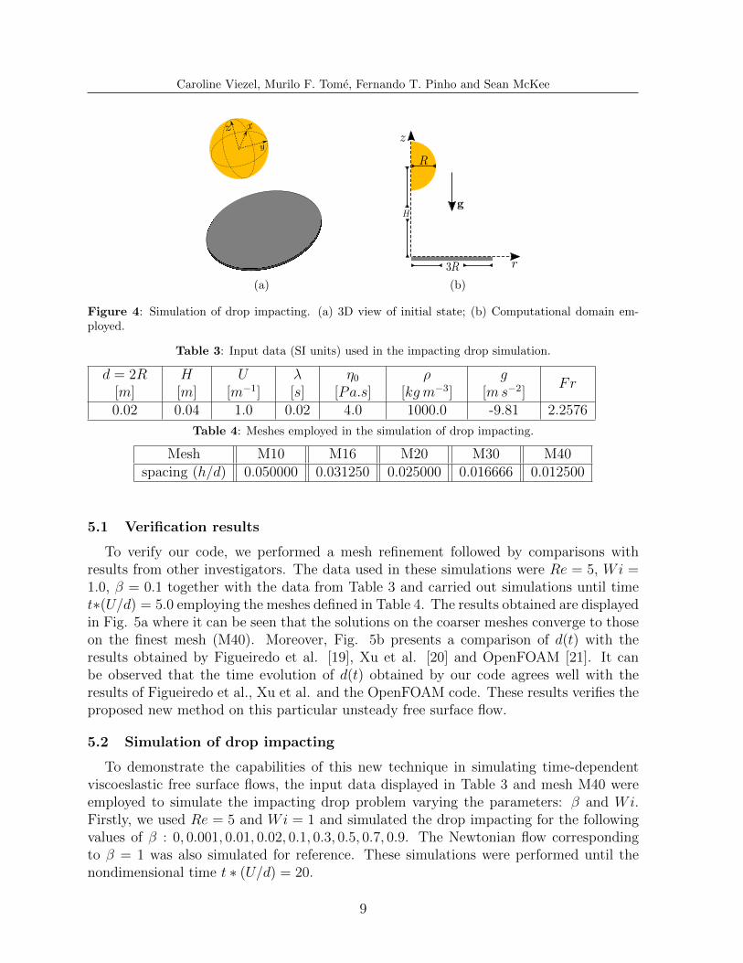
We considered a drop of diameter d = 2R that is positioned above a circular disk at aheight H (see Fig. 4b). At t = 0 the drop starts flowing downwards with initial velocityw(r, z, 0) = −U . After the drop impacts the disk it starts to flow radially expanding itsdiameter d(t) while, after a short period of time, due to elasticity forces, it is expectedthat it will contract, decreasing its diameter d(t). We are interest to study the effects ofthe parameters Wi and β on the variation of the drop diameter d(t) with time.

8


(a) (b)

Figure 4: Simulation of drop impacting. (a) 3D view of initial state; (b) Computational domain em-ployed.

Table 3: Input data (SI units) used in the impacting drop simulation.

d = 2R[m]

H[m]

U[m−1]

λ[s]

η0[Pa.s]

ρ[kg m−3]

g[ms−2]

Fr

0.02 0.04 1.0 0.02 4.0 1000.0 -9.81 2.2576

Table 4: Meshes employed in the simulation of drop impacting.

Mesh M10 M16 M20 M30 M40spacing (h/d) 0.050000 0.031250 0.025000 0.016666 0.012500

5.1 Verification results

To verify our code, we performed a mesh refinement followed by comparisons withresults from other investigators. The data used in these simulations were Re = 5, Wi =1.0, β = 0.1 together with the data from Table 3 and carried out simulations until timet∗(U/d) = 5.0 employing the meshes defined in Table 4. The results obtained are displayedin Fig. 5a where it can be seen that the solutions on the coarser meshes converge to thoseon the finest mesh (M40). Moreover, Fig. 5b presents a comparison of d(t) with theresults obtained by Figueiredo et al. [19], Xu et al. [20] and OpenFOAM [21]. It canbe observed that the time evolution of d(t) obtained by our code agrees well with theresults of Figueiredo et al., Xu et al. and the OpenFOAM code. These results verifies theproposed new method on this particular unsteady free surface flow.

5.2 Simulation of drop impacting

To demonstrate the capabilities of this new technique in simulating time-dependentviscoeslastic free surface flows, the input data displayed in Table 3 and mesh M40 wereemployed to simulate the impacting drop problem varying the parameters: β and Wi.Firstly, we used Re = 5 and Wi = 1 and simulated the drop impacting for the followingvalues of β : 0, 0.001, 0.01, 0.02, 0.1, 0.3, 0.5, 0.7, 0.9. The Newtonian flow correspondingto β = 1 was also simulated for reference. These simulations were performed until thenondimensional time t ∗ (U/d) = 20.

9


Figure 6a displays the time history of d(t) for each value of β. We can observe that theresults with β = 0.9 are similar to the Newtonian drop and show that after the drop im-pacted the disk, at time t ≈ 1.4, it continued to flow radially over the time, monotonicallyincreasing d(t). The results with β = 0.7, 0.5, 0.3 display a small expansion/contractionof the drop that occurred at times t ≈ 1.4 and t ≈ 2.4, respectively. It is seen that, afterthe contraction, the drop flowed radially, monotonically increasing d(t), similar to theNewtonian drop. For β = 0.1, 0.02, 0.01, 0.001, the behaviour of d(t) is more impressive.The higher elasticity within the drop makes it to expand/contract twice. These expan-sions/contractions become stronger as the value of β is reduced and for β = 0.001, thediameter d(t) is about the same as that obtained with the UCM model (β = 0). This isin agreement with the Oldroyd-B model as it reduces to the UCM model when β = 0.

To observe the effect of a high Weissenberg number on the spreading of the drop, severalsimulations using Re = 5.0, Wi = 20 and β = 0.01, 0.1, 0.3, 0.5, 0.7, 0.9 were performed.The evolutions of d(t) obtained in these simulations are displayed in Fig. 6b for each valueof β. It is seen that, after the drop impacted the disk, the values of d(t) corresponding toβ = 0.9, 0.7, 0.5, 0.3 increase monotonically in time and do not present any contraction.However, for β = 0.1, 0.01 the diameter d(t) presents large expansions, namely, d(t) > 2.5dfor β = 0.01 and d(t) > 2d at β = 0.1. An interesting point is that for these values of βthe diameter of the drop contracted to the same value of d(t) ≈ 0.04 = 2d.

To show that the surface of the drop undergoes large deformations during the freesurface flow, Fig. 7 displays a three-dimensional view of the unsteady flow of the dropover the disk for Re = 5, β = 0.01 and Wi = 1, 20. We can observe that the drop, withWi = 1 (see the left column with 3D visualisations), initially expands until time t = 2.6and from this time it retains contracting up to the time of t = 3.4 when an elevationat the centre of the drop can be seen (see the associated 3D view). After this time, thedrop again starts to expand, making its centre to undergo a depression at t ≈ 3.8 (see theassociated 3D view) and at a later time t = 4.6, due to a contraction, a small elevationoccurs at the centre of the drop. After this time the velocities within the drop becamesmall and the drop surface did not present any change. We believe that the effects ofexpansion/contraction are due to elastic forces acting within the drop.

The results obtained with Wi = 20 are more dramatic. The high elasticity of the fluidprovides more momentum to the drop so that its spreading is much more accentuated. Itis seen that after the maximum spread, at time t = 3.1, there is a thin layer of fluid overthe disk that is affected by elastic forces making the drop to contract until time t = 5.3when a small jet emerges from the drop. Afterwards, the drop starts to expand againspreading over the disk.

6 CONCLUSIONS

This work presented a novel numerical algorithm to solve the Oldroyd-B model forfree surface flows. The main feature of the formulation employed to solve the governingequations is the application of a splitting transformation that avoided the appearance ofthe viscosity ratio β in the momentum equations. The solution of the Oldroyd-B con-stitutive equation was obtained in terms of the conformation tensor A that was solved

10


implicitly. The method was verified against fully developed tube flow of Oldroyd-B flu-ids and convergence results were provided. The efficiency of this new methodology onunsteady free surface flow was attested by simulating the impacting drop problem forwhich mesh refinement and comparison with results from the literature were performed.The proposed method can easily be extended to three-dimensional flows and be used tosolve any viscoelastic flow where the usual rheological splitting of the extra-stress tensoris employed.

7 ACKNOWLEDGEMENTS

The authors would like to acknowledge the financial support given by the funding agen-cies: CNPq - Conselho Nacional de Desenvolvimento Cientıfico e Tecnologico Grant No.306280/2014-0 and 150282/2017-6, FAPESP Grant No. 2013/07375-0 (CEPID-CeMEAIproject) and CAPES Grant No. PROEX-9259544/D.

(a)

0 1 2 3 4 5

Dimensionless time

0.018

0.02

0.022

0.024

0.026

0.028

0.03

0.032

0.034

0.036

d(t

) [m

]

Mesh M40Figueiredo et al. [19]

Xu et al. [20]OpenFOAM [21]

(b)

Figure 5: Simulation of a drop impacting a disk - Re = 5, Wi = 1, β = 0.1. (a) Mesh refinement; (b)Comparison with other investigators. Our results were obtained on mesh M40.

0 5 10 15 20

Dimensionless time

0.018

0.02

0.022

0.024

0.026

0.028

0.03

0.032

0.034

0.036

0.038

d(t

) [m

] Newtonian β = 0.9

β = 0.7

β = 0.5

β = 0.3

β = 0.1

β = 0.02

β = 0.01

β = 0.001

β = 0.0

(a)

0 5 10 15 20

Dimensionless time

0.01

0.015

0.02

0.025

0.03

0.035

0.04

0.045

0.05

0.055

d(t

) [m

]

Newtonian β = 0.9

β = 0.7

β = 0.5

β = 0.3

β = 0.1

β = 0.01

(b)

Figure 6: Simulation of drop impacting a disk with Re = 5 and variation of β: (a) Wi = 1, (b) Wi = 20.

11


t = 2.2

t = 2.6

t = 3.1

t = 3.4

t = 3.8

t = 4.6

t = 5.3

t = 6.0

t = 7.5

t = 10.0

Figure 7: Simulation of a drop spreading over a disk - Re = 5, β = 0.01 and Wi = 1, 20, at selectedtimes (from top to bottom) t ∗ (U/d) = 2.2, 2.6, 3.1, 3.8, 4.6, 5.3, 6.0, 7.5, 10.0. 2D plots on the right andleft sides display the u-velocity where the blue colour refers to negative values and the red colour standsfor positive values.

12


REFERENCES

[1] R. G. Owens, T. N. Phillips, (2002). Computational Rheology. Imperial College Press.ISBN 978-1-86094-186-3.

[2] Oldroyd, James Clerk , On the Formulation of Rheological Equations of Estate,Proceedings of the Royal Society of London, Series A, Mathematical and PhysicalSciences, 200 (1950) (1063): 523-541.

[3] R. I. Tanner, A theory of die-swell, Journal of Polymer Science, 8 (1970), 2067-2078.

[4] H. Giesekus, A simple constitutive equation for polymer fluids based on the con-cept of deformation-dependent tensorial mobility, Journal of Non-Newtonian FluidMechanics, 11 (1982), 69-109.

[5] R. B. Bird , R. C. Armstrong, O. Hassager, Dynamics of Polymeric Liquids, vol. 2,Wiley, New York, 1987.

[6] T. C. B. McLeish, R. G. Larson, Molecular constitutive equations for a class ofbranched polymers: The pom-pom polymer, Journal of Rheology, 42 (1998), 81-

[7] W. M. H. Verbeeten, G. W. M. Peters, F. P. T. Baaijens, Differential constitutiveequations for polymer melts: the extended Pom-Pom model, Journal of Rheology,45 (2001), 823-843.

[8] A. C. Papanastasiou, L. E. Scriven, C. W. Macosko, An integral constitutive equationfor mixed flows: viscoelastic characterization, Journal of Rheology, 27 (1983), 387-410.

[9] X. L. Luo, E. Mitsoulis, An efficient algorithm for strain history tracking in finiteelement computations of non-Newtonian fluids with integral constitutive equations,International Journal for Numerical Methods in Fluids, 11 (1990), 1015-1031.

[10] M. J. Crochet, R. Keunings, Die swell of a Maxwell fluid: numerical prediction,Journal of Non-Newtonian Fluid Mechanics, 7 (1980), 199-212.

[11] M. J. Crochet, R. Keunings, Finite element analysis of die swell of a highly elasticfluid, Journal of Non-Newtonian Fluid Mechanics 10 (1982), 339-356.

[12] V. Delvaux, M. J. Crochet, Numerical simulation of delayed die swell, RheologicaActa, 29 (1990), 1-10.

[13] C. M. Oishi, M. F. Tome, Jose A. Cuminato, S. McKee, An implicit technique forsolving 3D low Reynolds number moving free surface flows, Journal of ComputationalPhysics, 227 (2008), 7446-7468.

[14] A. Bonito, M. Picasso, M. Laso, Numerical simulation of 3D viscoelastic flows withfree surfaces, JCP (215 (2006), 691-716.

13


[15] M. A. Alves, P. Oliveira, F. Pinho, A convergent and universally bounded interpo-lation scheme for the treatment of advection, International Journal for NumericalMethods in Fluids, 41 (2003), 47-75.

[16] M. F. Tome, L. Grossi, , A. Castelo, J. A. Cuminato, S. McKee, K. Walters, Die-swell, splashing drop and a numerical technique for solving the Oldroyd B model foraxisymmetric free surface flows, Journal of Non-Newtonian Fluid Mechanics, 141,(2007), 148-166.

[17] M. F. Tome, A. Castelo, J. Murakami, J. A. Cuminato, R. Minghin, M. C. F. Oliveira,N. Mangiavacchi, S. McKee, Numerical simulation of Axisymmetric free surface flows,Journal of Computational Physics, 157 (2000), 441-472.

[18] J. Peng, K.-Q. Zhu, Instability of the interface in co-extrusion flow of two UCMfluids in the presence of surfactant, Journal of Non-Newtonian Fluid Mechanics, 166(2011), 152-163.

[19] R. A. Figueiredo, C. M. Oishi, J. A. Cuminato, J. C. Azevedo, A. M. Afonso, M. A.Alves, Numerical investigation of three dimensional viscoelastic free surface flows:impacting drop problem, Proceedings of 6th European Conference on Computa-tional Fluid Dynamics (ECFD VI), E. Onate, J. Oliver and A. Huerta (Eds), 2014,Barcelona, Spain.

[20] Xi. Xu, J. Ouyang, T. Jiang, Q. Li, Numerical simulation of 3D-unsteady viscoelasticfree surface flows by improved smoothed particle hydrodynamics method, Journal ofNon-Newtonian Fluid Mechanics, 177-178, (2012), 109-120.

[21] H. Jasak, A. Jemcov, Z. Tukovic, OpenFOAM: a C++ library for complex physicssimulations, International Workshop on Coupled Methods in Numerical Dynamics,IUC Dubrovnik, Croatia, 2007, 1-20.

[22] D. Rajagopalan, R. C. Armstrong, R. A. Brown, Finite Element Methods for cal-culating of steady, viscoelastic flow using constitutive equations with a newtonianviscosity, J. Non-Newtonian Fluid Mechanics, 36 (1990), 159-192.

[23] Xiaoyang Xu, Xiao-Long Deng, An improved weakly compressible SPH method forsimulating free surface flows of viscous and viscoelastic fluids, Computer PhysicsCommunications, 201 (2016), 43-62.

[24] A. J. Chorin, Numerical solution of the Navier-Stokes equations, Mathematics ofComputation, 22 (1968), 745-762, DOI: https://doi.org/10.1090/S0025-5718-1968-02423.

[25] M. F. Tome, B. Duffy, S. McKee, A numerical technique for solving unsteady non-Newtonian free surface flows, Journal of Non-Newtonian Fluid Mechanics, 62 (1996),9-34.

14

a numerical technique for solving the oldroyd-b model …

Documents