A numerical strategy to compute optical parameters inturbulent flow. Application to telescopes

Ramon Codina1,∗, Joan Baiges1, Daniel Perez-Sanchez1 and Manuel Collados2

1 International Center for Numerical Methods in Engineering (CIMNE),Universitat Politecnica de Catalunya, Jordi Girona 1-3, Edifici C1, 08034 Barcelona, Spain.

2 Instituto de Astrofısica de Canarias, Via Lactea s/n, 38205 La Laguna, Tenerife, Spain.∗ ramon.codina@upc.edu

Contents1 Introduction 2

2 The aerodynamic problem 42.1 Problem statement . . . . . . . . . . . . . . . . . . . . . . . . . . . . . . . . . . . . . . . . . . . . . . . . 42.2 Finite element approximation . . . . . . . . . . . . . . . . . . . . . . . . . . . . . . . . . . . . . . . . . . 52.3 Some implementation issues . . . . . . . . . . . . . . . . . . . . . . . . . . . . . . . . . . . . . . . . . . . 7

3 Optical parameters 73.1 Physical background . . . . . . . . . . . . . . . . . . . . . . . . . . . . . . . . . . . . . . . . . . . . . . . 73.2 Numerical strategy . . . . . . . . . . . . . . . . . . . . . . . . . . . . . . . . . . . . . . . . . . . . . . . . 10

4 An example of application 12

5 Concluding remarks 21

1

Abstract

We present a numerical formulation to compute optical parameters in a turbulent air flow. Thebasic numerical formulation is a large eddy simulation (LES) of the incompressible Navier-Stokesequations, which are approximated using a finite element method. From the time evolution of theflow parameters we describe how to compute statistics of the flow variables and, from them, theparameters that determine the quality of the visibility. The methodology is applied to estimate theoptical quality around telescope enclosures.

1 Introduction

In spite of its impact in some applications, the problem of estimating the optical properties in a turbulentflow is not particularly popular in the computational fluid dynamics (CFD) community. An examplewhere this problem is of paramount importance is in the determination of the location where largetelescope facilities have to be built. The purpose of this paper is precisely to explain the problem and topropose a numerical formulation to approximate it.

The location for the construction of a telescope depends on several factors, some of them of logisticnature (such as the ease of construction or the scientific and political environment) and others, obvi-ously, directly relevant to the quality of the astronomical observation. Among the latter, periods of goodvisibility (without clouds), weather conditions or the proximity to the Equator (leading to the so calledsky quality) have an obvious impact. However, at least as important as those are the optical propertiesof the environment where the telescope enclosure is placed, primarily determined by the aerodynamicbehavior of this enclosure.

The effect of the air dynamics around the telescope building on the visibility is due to the wavenature of light. Light rays, as the visible portion of the electromagnetic spectrum, travel at the lightspeed and with a wavelength between 400 and 800 nanometers in the vacuum. However, when theyenter a transparent medium, such as the earth atmosphere, they decrease their speed, therefore changingtheir wavelength (the frequency is kept). The ratio between the speed of light in the vacuum and in amedium is the so called refractive index of this medium, that we will denote as usual by n.

For a single beam of light, if this beam is not orthogonal to the medium interface, refraction occurs.In a medium in which the refractive index changes from point to point, the direction of the beam of lightsuffers continuous changes. However, the problem arises when different light rays forming a wavefrontenter a medium with variable refractive index. The variability of this index causes the different rays torefract in a different way, thus leading to wavefront distortion and a deterioration of the quality of thevisibility.

The problem thus is the variability of the refractive index in the atmosphere rather than the refractiveindex itself. Here is where turbulence comes into the picture. Turbulence fluctuations, particularly intemperature, induce fluctuations in the refractive index that lead to visibility deterioration.

A first and classical approach to determine the feasibility of a certain site as a telescope locationhas been to quantify turbulence in the region, usually by experimental means. Classical turbulenceparameters, such as the integral length, turbulence intensity or turbulence energy spectra have provedto be useful to assess the quality of a site to build a telescope. However, arguments derived from thisinformation are merely qualitative, giving for granted that the higher the turbulence effects, the lowerthe visibility quality.

That CFD may play a role in this problem is obvious from what has been explained. The idea wouldsimply be to replace experimental data by results of numerical simulations. In fact, the qualitativelink between turbulence and optical quality led the International Center for Numerical Methods inEngineering (CIMNE) to participate in several projects related to the aerodynamic analysis of telescopebuildings in collaboration with the Astrophysical Institute of the Canary Islands (IAC). In particular,

2

CIMNE has been involved in the aerodynamic analysis of the GTC telescope [12] and in the ELTproject from the European Commission [10], as well as in the analysis of the ATST project of a solartelescope [1]. In this last case we have considered the possibility to go further, and to quantify the effectof turbulence in the visibility quality rather than simply computing the turbulence parameters.

In the astrophysical community, optical quality is measured, among other parameters, by the socalled Fried parameter r0 and the Greenwood frequency fG (see [3, 22, 24] for background in theoptical concepts to be used). Roughly speaking, the former corresponds to the diameter of a circlewhere the mean distortion expected of a light wavefront is 1 radian, whereas the latter gives an idea ofthe temporal frequency at which refraction varies. Both are essential in adaptive optics in astronomy.They are used to design segmented telescopes (the size of the segments being determined by the Friedparameter) and their actuators in typical active control systems of these devices.

The question is whether r0 and fG can be computed or not. If one assumes that the air flow isfully turbulent, the answer is positive. For length scales in the inertial range of the Kolmogorov energycascade, it turns out that these parameters can be expressed in terms of the structure function of therefractive index and, under an isotropy assumption, by the square of the so called constant of structure,C2

n . This is, therefore, the scalar field that needs to be computed which, according to the previousdiscussion, must be related to the turbulence fluctuations. This dependence can be finally expressed as arelationship between C2

n and the mean pressure and the constant of structure of the temperature, which,in turn, depends on the gradients of the mean temperature and mean velocities. The conclusion is thusclear: If we are able to compute mean flow quantities (pressure, temperature and velocity) in a fullydeveloped turbulent flow, we will be able to estimate the constant of structure of the refractive indexand, from integration along the optical path of the light beam, the Fried parameter and the Greenwoodfrequency. These parameters need to be computed for all directions of observation of interest.

Once the model to compute the optical parameters is established (and accepted) the success dependson the CFD simulation to obtain mean flow quantities. However, now they are needed not only to es-tablish a mere qualitative indication of the optical quality, but to compute a quantitative measure of thisquality. The first and essential point to consider is that all the expressions to be used are derived underthe assumption that the flow lies within the inertial range. The classical statistical temporal and spa-tial correlations between velocity components, pressure and temperature need to apply. This excludesfrom the very beginning the use of RANS (Reynolds averaged Navier-Stokes) models and restricts thealternatives to, at least, LES (large eddy simulation) formulations.

As basic numerical formulation for the aerodynamic problem we have used a stabilized finite ele-ment method for the spatial discretization together with a second order time integration scheme. TheSmagorinsky model has been used as LES formulation, even though richer dynamics and still gen-uine turbulent behavior are obtained if the stabilization alone is let to act as turbulence model. Boththe numerical formulation and the LES model are described in Section 2. Once the flow variables arecomputed and time averaged, the square of the constant of structure of the refractive index can be ob-tained. From these results one may now compute the Fried parameter and the Greenwood frequency byintegration of functions that depend on Cn along different optical paths corresponding to the directionsof observation of interest. A detailed description of how to perform these calculations is presented inSection 3.

As an example of application of the strategy presented, we have applied it to the ATST telescopementioned earlier in Section 4. We believe this example may serve to understand the potential of CFDin the field of the optical environmental quality, which in the case of telescopes is crucial to select thesite of these scientific installations. Some concluding remarks close the paper in Section 5.

3

2 The aerodynamic problem

2.1 Problem statement

In this section we shall consider the flow problem for an incompressible fluid taking into account thecoupling of the Navier-Stokes equations with the heat transport equation through Boussinesq’s assump-tion, as well as a nonlinear viscosity dependence on the velocity gradient invariants through Smagorin-sky’s LES model. Some comments will be made later on about the possibility to avoid turbulencemodeling and to rely only on the numerical formulation.

The equations describing the problem are

∂tu+ (u · ∇)u− 2∇ · [νε(u)] +∇p+ βgϑ = f , (1)

∇ · u = 0, (2)

∂tϑ+ (u · ∇)ϑ−∇ · (κ∇ϑ) = 0, (3)

to be solved in Ω× (0, tfin), where Ω ⊂ R3 is the computational domain and [0, tfin] is the time interval

to be considered. In (1)-(3), u denotes the velocity field, p is the kinematic pressure (i.e., the pressuredivided by the density), ϑ is the temperature, ν is the total kinematic viscosity (physical plus turbulent),ε(u) is the symmetrical part of the velocity gradient, β is the thermal expansion coefficient, g is thegravity acceleration vector, f is the vector of body forces, and κ is the total thermal diffusivity (that is,the physical plus turbulent thermal conductivity divided by the heat capacity). The density ρ0 is assumedconstant to obtain equations (1)-(3). In the numerical example of Section 4, all these properties havebeen taken as those corresponding to air in normal conditions.

The force vector f in (1) contains the reference buoyancy forces from Boussinesq’s assumption,that is

f = g(1 + βϑ0).

In this equation, ϑ0 is the reference temperature from which buoyancy forces are computed.Smagorinsky’s turbulence model has been employed in the numerical simulations (see, e.g. [20, 23,

9] for background). This model is tight to the numerical discretization in space of the flow equations,which in our case is performed using the finite element method. The turbulent kinematic viscosityassociated to this model is

νtur = ρ−10 ch2 [ε(u) : ε(u)]1/2 ,

where c is a constant, usually taken as c = 0.01, the colon stands for the double contraction of secondorder tensors and h is the length of the element of the finite element discretization described later wherethe turbulent kinematic viscosity is to be computed. The total viscosity will be ν = νmol + νtur, νmol

being the molecular viscosity.Concerning the turbulent thermal diffusivity, it is taken of the form

κtur = Prturνtur, (4)

where Prtur is the turbulent Prandtl number, taken as Prtur = 1 in the numerical example. The totalthermal diffusivity will be κ = κmol + κtur, κmol being the molecular thermal diffusivity.

In order to write the boundary conditions for equations (1)-(3), consider the boundary Γ = ∂Ωsplit into sets of disjoint components as Γ = Γdv ∪ Γnv ∪ Γmv and also as Γ = Γdt ∪ Γnt, where Γdvand Γdt are the parts of the boundary with Dirichlet type boundary conditions for the velocity and thetemperature, respectively, and Γnv and Γnt are those where Neumann type conditions are prescribed.

4

Mixed boundary conditions for the velocity are fixed on Γmv. If the Cauchy stress tensor (divided bythe density) is written as σ = −pI +2νε(u), the exterior normal to ∂Ω is n, and prescribed values arerepresented by an overbar, the boundary conditions to be considered are

u(x, t) = u(x, t) on Γdv, (5)

n · σ(x, t) = 0 on Γnv, (6)

n · u(x, t) = 0 and n · σ(x, t)|tang = t on Γmv, (7)

ϑ(x, t) = ϑ(x, t) on Γdt, (8)

κn · ∇ϑ(x, t) = 0 on Γnt, (9)

for t ∈ (0, tfin). In (7), n · σ(x, t)|tang denotes the component of the stress vector n · σ(x, t) tangentto ∂Ω and t is the stress resulting from the standard wall law (see for example [20])

t = −ρ0U2∗

|u|u,

where U∗ is the solution of the nonlinear equation

|u|

U∗

=1

Klog

(

U∗∆

ν

)

+ C,

with K = 0.41 (von Karman constant), C = 5.5 and where ∆ is the distance from the wall at whichthe velocity is evaluated.

To close the problem, initial conditions have to be appended to equations (1)-(3) and the boundaryconditions (5)-(9). They are of the form u(x, 0) = u0(x), ϑ(x, 0) = ϑ0(x) for x ∈ Ω, where u0(x) isa given initial velocity and ϑ0(x) a given initial temperature.

In the numerical simulations of the telescope building, Γdv corresponds to the inflow part of theboundary of the computational domain, where the wind velocity is prescribed to a certain value ofinterest and with a given direction, whereas Γnv is the outflow boundary. The surface Γmv correspondsto both the ground surface and the building surface.

2.2 Finite element approximation

In order to discretize in space problem (1)-(3), let Ωe be a finite element partition of the domain Ω,with index e ranging from 1 to the number of elements nel. We denote with a subscript h the finiteelement approximation to the unknown functions, and by vh, qh and ψh the velocity, pressure andtemperature test functions associated to Ωe, respectively.

A very important point is that we are interested in using equal interpolation for all the unknowns(velocity, pressure and temperature). Therefore, all the finite element spaces are assumed to be built upusing the standard continuous interpolation functions. In particular, all the numerical simulations havebeen carried out using meshes of linear tetrahedra.

In order to overcome the numerical problems of the standard Galerkin method, a stabilized finiteelement formulation is applied. This formulation is presented in [6]. It is based on the subgrid scaleconcept introduced in [15], although when linear elements are used it reduces to the Galerkin/least-squares method described for example in [11] (see also [25]). We apply this stabilized formulationtogether with a finite difference approximation in time. The bottom line of the method is to test thecontinuous equations by the standard Galerkin test functions plus perturbations that depend on theoperator representing the differential equation being solved. In our case, this operator corresponds to

5

the linearized form of the Navier-Stokes equations (1)-(2) and the heat equation (3). In this case, themethod consists of finding uh, ph and ϑh such that

∫

Ω

vh · ru1 dx+

∫

Ω

2ε(vh) : νε(uh) dx−

∫

Ω

ph∇ · vh dx

+

nel∑

e=1

∫

Ωe

ζu1 · (ru1 + ru2) dx+

nel∑

e=1

∫

Ωe

ζu2 rp dx

=

nel∑

e=1

∫

Ωe

(vh + ζu1) · f dx+

∫

Γmv

vh · t dΓ,

∫

Ω

qhrp dx+

nel∑

e=1

∫

Ωe

ζp · (ru1 + ru2) dx =

nel∑

e=1

∫

Ωe

ζp · f dx,

∫

Ω

ψh · rϑ1 dx+

∫

Ω

κ∇ψh · ∇ϑh dx+

nel∑

e=1

∫

Ωe

ζϑ (rϑ1 + rϑ2) dx = 0,

for all test functions vh, qh and ψh, where

ru1 := ∂tuh + gβϑh + (uh · ∇)uh, (10)

ru2 := −2∇ · [νε(uh)] +∇ph, (11)

rp := ∇ · uh, (12)

rϑ1 := ∂tϑh + (uh · ∇)ϑh, (13)

rϑ2 := −∇ · (κ∇ϑh) , (14)

the functions ζu1, ζu2 and ζp are computed within each element as

ζu1 = τu (uh · ∇)vh + 2∇ · [νε(vh)] , (15)

ζu2 = τp∇ · vh, (16)

ζp = τu∇qh, (17)

ζϑ = τϑ [(uh · ∇)ψh +∇ · (κ∇ψh)] , (18)

and the parameters τu, τp and τϑ are also computed element-wise as (see [6])

τu =

[

4ν

h2+

2|uh|

h

]

−1

,

τp = 4ν + 2|uh|h,

τϑ =

[

4κ

h2+

2|uh|

h

]

−1

,

where h is the element size for linear elements and half of it for quadratics.From (15)-(18) it is observed that these terms are precisely the adjoints of the (linearized) operators

of the differential equations to be solved applied to the test functions (observe the signs of the viscousterm in (15) and of the diffusive term in (18)). This method corresponds to the algebraic version ofthe subgrid scale approach ([15]) and circumvents all the stability problems of the Galerkin method. Inparticular, in this case it is possible to use equal velocity pressure interpolations, that is, we are not tightto the satisfaction of the inf-sup stability condition.

A controversial issue is whether the stabilized formulation presented is able to act as a turbulencemodel, that is to say, if the Smagorinsky viscosity can be turned off. This possibility is advocated in[8, 2]. Even though our numerical simulations have been performed using the Smagorinsky model,some runs without it have provided good results with richer dynamics.

6

2.3 Some implementation issues

Apart from a more or less standard iterative procedure to deal with the different nonlinearities, the basicnumerical formulation presented above has been implemented using some features which will not bedetailed here. These are:

• Time integration can be performed with any finite difference scheme. In particular, the exampleof Section 4 has been simulated using the second order Crank-Nicolson method.

• Nodal based implementation [5]. This implementation is based on an a priori calculation of theintegrals appearing in the formulation and then the construction of the matrix and right-hand-sidevector of the final algebraic system to be solved. After appropriate approximations, this matrixand this vector can be constructed directly for each nodal point, without the need to loop overthe elements and thus making the calculations much faster. In order to be able to do this, all thevariables have to be defined at the nodes of the finite element mesh, not on the elements. This isalso so for the stabilization parameters of the formulation.

• Block-iterative coupling to segregate the velocity-pressure and temperature calculations [4]. Asingle iterative loop is used to deal both with the nonlinearities of the problem and with thetemperature coupling with the Navier-Stokes equations.

• Predictor corrector scheme [7]. The pressure segregation is inspired in fractional step schemes,although the converged solution corresponds to that of a monolithic time integration.

The reader is referred to the references indicated in each item for details.

3 Optical parameters

In this section we introduce the parameters that allow us to measure the quality of the seeing of a site,and we also describe their numerical approximation in the context of the finite element formulation forthe flow equations presented above.

3.1 Physical background

The optical parameters we are interested in are the Fried parameter and the Greenwood frequency. Infact, they are both obtained from integration of a function of the structure constant of the refractiveindex along an optical path. Let us start describing the problem and leave for the next subsection itsapproximation (see [22] for more details).

Let n(x, t) be the refractive index of a medium. Optical quality depends on spatial and temporalvariability of this parameter, basically due to temperature and humidity fluctuations. In particular, weare interested in the structure function of n, defined as

Dn(x,x′) = 〈[n(x, t)− n(x′, t)]2〉. (19)

Here, 〈·〉 denotes the ensemble average. However, under the ergodicity assumption we will replace it, in(19) and below, by the time average over a time window of period T , large enough to make Dn(x,x

′)(almost) time independent. Likewise, we will assume isotropic turbulence, so that Dn depends only onr := |x− x′|, not on x′. This dependence will be written as Dn(x, r). Moreover, if we assume further

7

that 1/r belongs to the inertial range of the Kolmogorov spectrum, it can be shown by dimensionalanalysis that (see [24])

Dn(x, r) = C2n(x)r

2/3, (20)

where Cn(x) is the constant of structure of n. See also [26] for a discussion about the limits of thisapproximation.

Given a point x ∈ Ω, let us consider a beam of light arriving to x with the direction given by a unitvector l. To integrate along this beam of light, we may consider it starting from rather than arrivingto x, and parametrize it as x + sl, with s ∈ [0,∞). Having introduced this notation, the optical pathlength δl and the phase fluctuation ϕl can be computed as

δl(x, t) =

∫

∞

0

n(x+ sl, t)ds, ϕl(x, t) =2π

λ

∫

∞

0

n(x+ sl, t)ds, (21)

where λ is the wavelength of the wavefront of the light beam. Note that subscript l refers to the directionof the light beam.

To obtain the variability of ϕl (and therefore the relative change in the wave phase) its structurefunction is needed. It is given by

Dϕl(x, ξ) = 〈[ϕl(x, t)− ϕl(x+ ξ, t)]2〉,

where ξ = |ξ|. Making use of (21) and (20) it can be shown that (see [22])

Dϕl(x, ξ) = 2.91

(

2π

λ

)2

ξ5/3∫

∞

0

C2n(x+ sl)ds.

This expression can be written in terms of the Fried parameter r0 as

Dϕl(x, ξ) = 6.88

(

ξ

r0

)5/3

,

where

r0 = r0(l;x) =

(

16.6

λ2

∫

∞

0

C2n(x+ sl)ds

)

−3/5

. (22)

Note that once again we have made explicit the dependence of r0 on the spatial point and the light beamdirection. Obviously, it also depends on the wavelength of the light wave, λ.

The importance of r0 is due to the fact the mean-square distortion of a wavefront over a circle ofarea A and diameter d centered at a point x, normal to l, parametrized by x+ y and given by

σ21 = σ21(l;x) =4

πd2

∫

A〈[ϕl(x+ y, t)− ϕ0,l(x, t)]

2〉dy,

ϕ0,l(x, t) :=4

πd2

∫

Aϕl(x+ y, t)dy,

can be shown to be (see [22])

σ21 = 1.03

(

d

r0

)5/3

.

Thus, if d = r0 the root-mean-square (RMS) distortion is approximately 1 radian.

8

The Fried parameter r0 is essential in adaptive optics. In the case of telescopes it allows to determinethe number of segments into which a segmented mirror has to be split, or the distance between actuatorsfor a continuous deformable mirror, by prescribing an admissible RMS distortion of a wavefront [3]. Butthe design of their actuators is also based on the so called Greenwood frequency, which is an indicationof how fast the atmosphere is changing and defines the bandwidth of the servo control for an adaptiveoptics system. This frequency is defined as

fG = 0.43Vwindr0

(23)

where Vwind is a weighted mean wind velocity defined as

Vwind = Vwind(l;x) =

(

∫

∞

0〈|u|〉5/3C2

n(x+ sl)ds∫

∞

0C2

n(x+ sl)ds

)3/5

. (24)

The problem of computing r0 and fG is reduced to the problem of computing the structure functionof the refractive index, Cn, and then computing the integrals in (22) and (24). In turn, this structurefunction can be related to the structure function of the temperature, the humidity and their joint structureparameter (see [19]). However, we will consider the humidity effects negligible. Thus, if we write thetemperature dependence of n as n = n(ϑ), we have

Cn =dn

dϑCϑ,

where Cϑ is the structure function of the temperature. Assuming pressure equilibrium it is foundthat [24]

Cn =79× 10−6

〈ϑ〉2〈p〉Cϑ, (25)

where p is assumed to be measured in millibars and ϑ is the absolute temperature. Here and below, ϑ,p and u denote the solution of the continuous problem without using a LES model, that is to say, withνtur = 0, κtur = 0 in (1)-(3).

In view of (25), the problem is to compute Cϑ. Once again in the inertial range of the Kolmogorovspectrum and assuming the temperature to be a passive quantity, it can be shown that (see [22])

C2ϑ = a2χε−1/3, (26)

where a is an empirical value called Obukhov-Corrsin constant (see [14, 27] for extensions and a dis-cussion about Obukhov-Corrsin constants and on the validity of this approximation). In (26), χ denotesthe mean thermal diffusive dissipation and ε the mean dissipation of kinetic energy of the flow. Theseparameters are given by

χ := κmol〈|∇ϑ|2〉, ε := νmol〈|ε(u)|

2〉. (27)

The problem is now closed: using (27) in (26) and the result back in (25) we have an expression tocompute Cn in terms of the flow variables u, p, ϑ at each point.

The question now is how to apply this development in the context of a LES simulation and, moreprecisely, using the flow variables uh, ph, ϑh resulting from the finite element approximation of aLES model as described in the previous section. The first point to consider is that filtered unknowns

9

appearing in a LES model need to maintain the mean of the original variables. Assuming this to holdalso for their finite element approximation we have that

〈u〉 ≈ 〈uh〉, 〈p〉 ≈ 〈ph〉, 〈ϑ〉 ≈ 〈ϑh〉. (28)

The second point is that the dissipation of the continuous problem is approximately equal to the dissi-pation of the LES approximation using the effective turbulent thermal diffusion, in the case of the heatdissipation, or effective turbulent kinematic viscosity, in the case of the mechanical dissipation. Thisis in fact the main requirement posed by Lilly to LES models [17, 20], and the key feature for theirdesign [9]. Moreover, it is also shown in [13] that the numerical formulation presented in Section 2introduces also a mechanical numerical dissipation proportional to the viscous dissipation. This leadsus to assume that

κmol〈|∇ϑ|2〉 ≈ κtur〈|∇ϑh|

2〉, νmol〈|ε(u)|2〉 ≈ νtur〈|ε(uh)|

2〉. (29)

Using approximations (28) and (29) in (26) and inserting the result in (25) it is found that

Cn = 79× 10−6〈ϑh〉−2 〈ph〉 a ν

1/3tur 〈|∇ϑh|

2〉1/2〈|ε(uh)|2〉−1/6, (30)

where we have assumed that Prtur = 1 in (4). Equation (30) is the expression we were looking for.It allows us to compute the structure function of the refractive index in terms of the flow variablesresulting from a LES numerical simulation. Using this expression in (22) and in (24), also replacing uby uh in this last case, the Fried parameter and the Greenwood frequency can be computed. We presentnext the algorithm to compute the integrals in (22) and (24).

3.2 Numerical strategy

Expression (30) allows us to compute the structure constant of the refractive index at each node ofthe finite element mesh introduced in Section 2 to approximate the flow equations. The only remarkis that the derivatives of uh appearing in ε(uh) and the derivatives of ϑh appearing in ∇ϑh will bediscontinuous, usually computed at the numerical integration points. They can be approximated bycontinuous functions by using a classical L2 projection. To simplify the exposition, we will assume thatthis approximation is done, although it is not necessary (and in fact we have not used it in the numericalexample).

Equations (22) and (24), with the continuous functions approximated by finite element functionsdefined at the nodes of the finite element mesh, imply an integral along the light beam. Therefore, ourconcern now is to compute integrals of the form

I(l;x) =

∫

∞

0

Fh(x+ sl)ds, (31)

where the finite element function Fh(x) is an approximation to C2n in the case of (22) and the denom-

inator in (24) and an approximation to 〈|u|〉5/3C2n in the case of the numerator in (24). Note that Fh

would be discontinuous across interelement boundaries if ε(uh) and ∇ϑh are not approximated bycontinuous functions.

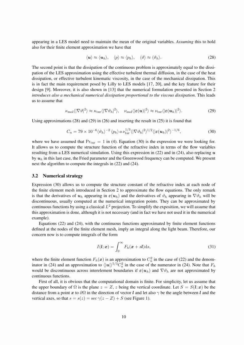
First of all, it is obvious that the computational domain is finite. For simplicity, let us assume thatthe upper boundary of Ω is the plane z = Z, z being the vertical coordinate. Let S = S(l;x) be thedistance from a point x to ∂Ω in the direction of vector l and let also γ be the angle between l and thevertical axes, so that s = s(z) = sec γ(z − Z) + S (see Figure 1).

10

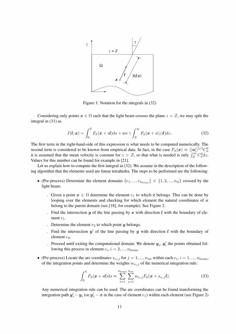
Figure 1: Notation for the integrals in (32)

Considering only points x ∈ Ω such that the light beam crosses the plane z = Z, we may split theintegral in (31) as

I(l;x) =

∫ S

0

Fh(x+ sl)ds+ sec γ

∫

∞

ZFh(x+ s(z)l)dz. (32)

The first term in the right-hand-side of this expression is what needs to be computed numerically. Thesecond term is considered to be known from empirical data. In fact, in the case Fh(x) ≈ 〈|u|〉

5/3C2n

it is assumed that the mean velocity is constant for z > Z, so that what is needed is only∫

∞

Z C2ndz.

Values for this number can be found for example in [21].Let us explain how to compute the first integral in (32). We assume in the description of the follow-

ing algorithm that the elements used are linear tetrahedra. The steps to be performed are the following:

• (Pre-process) Determine the element domains e1, ..., enbeam ∈ 1, 2, ..., nel crossed by the

light beam:

. Given a point x ∈ Ω determine the element e1 to which it belongs. This can be done bylooping over the elements and checking for which element the natural coordinates of xbelong to the parent domain (see [18], for example). See Figure 2.

. Find the intersection y of the line passing by x with direction l with the boundary of ele-ment e1.

. Determine the element e2 to which point y belongs.

. Find the intersection y′ of the line passing by y with direction l with the boundary ofelement e2.

. Proceed until exiting the computational domain. We denote yi, y′

i the points obtained fol-lowing this process in element ei, i = 2, ..., nbeam.

• (Pre-process) Locate the arc coordinates sei,j for j = 1, ..., nint within each ei, i = 1, ..., nbeam,of the integration points and determine the weights wei,j of the numerical integration rule:

∫ S

0

Fh(x+ sl)ds ≈

nbeam∑

i=1

nint∑

j=1

wei,jFh(x+ sei,jl). (33)

Any numerical integration rule can be used. The arc coordinates can be found transforming theintegration path y′i − yi (or y′1 −x in the case of element e1) within each element (see Figure 2)

11

to the reference interval of the particular integration rule. For example, for the Gauss-Legendrerule used in the numerical simulation of the following section, if sei,0 is the arc coordinate ofpoint yi for element ei,

sei,j = sei,0 +1

2(1 + ηj)|y

′

i − yi|, wei,j =1

2|y′i − yi|ωj , j = 1, ..., nint,

where ηj and ωj are the coordinates and weights of the j-th integration point in the interval[−1, 1].

• (Post-process) Once the LES simulation has finished, obtain the nodal values of the time averagedflow variables and, from them, the nodal values of Fh(x) (if derivatives are not approximated bycontinuous functions, Fh will be discontinuous).

• (Post-process) Interpolate from the nodes of each element to the numerical integration points andperform the numerical integral (33).

Figure 2: Line integration within an element. The crosses denote the numerical integration points.

4 An example of application

In this section we present an application of the numerical strategy described in the previous sectionsto the calculation of the Fried parameter and Greenwood frequency around a telescope. The exampleto be shown corresponds to the project of a solar telescope, the Advanced Technology Solar Telescope(ATST) [1], in which study the Astrophysical Institute of the Canary Islands has been involved. Theresults to be presented do not correspond to a real situation, but to a preliminary analysis to determinethe convenience of the project. Their purpose is not an exact quantitative analysis of the problem, but aqualitative demonstration of the possibilities of the formulation proposed herein.

The physical properties used in the numerical approximation of (1)-(3) are those of air at normalconditions.

The site to be analyzed is located in the observatory of El Roque de los Muchachos, in the LaPalma island of the Canary archipelago. Figure 3 shows a general view of the site with the surface finiteelement mesh used to discretize what we will call the large computational domain. This domain is usedfor a preliminary simulation used to determine the boundary conditions of a more detailed calculation.

12

The region of the island analyzed has 10 × 7.6 km2 and a height of 1400 m above the sea level. Asemisphere of radius 14.2 km is the computational domain (see Figure 3). The mesh used has only9.2 × 104 linear tetrahedral elements. Steady-state calculations (understood as a Reynolds averagedNavier-Stokes simulations) have been performed with different wind directions and wind intensities,considered representative of the site. In the following, only results corresponding to a uniform wind of 4m/s coming from the west will be considered. In upper atmospheric layers, this wind is not perturbed,while near the ground its direction and speed are altered by the terrain geometry and buildings. Thevelocity of 4 m/s is imposed as boundary condition at the inflow nodes of the spherical computationaldomain mentioned.

Figure 3: General view and detail of the large scale computational domain

Results obtained for the large computational region are used as boundary conditions for the smallscale domain where the simulations will be actually carried out, now introducing the ATST telescopeas well as the other existing buildings hosting telescopes. Only results for one of the sites analyzed willbe shown. The extension of the small computational domain has 1217000 m2 and it is discretized usinga mesh of 3.2 × 106 linear tetrahedral elements (see Figure 4). It corresponds to a sphere of diameter28450 m, the minimum distance from the telescope to the boundary being 12500 m.

As it has been mentioned, velocity boundary conditions for the small scale domain are obtainedfrom the large scale domain. Standard interpolation between meshes is used. Concerning the tempera-ture, we have assumed a near ground temperature profile in the vertical coordinate z of the form

T = T0 − Tdeclog z − log zh

logH − log zh, z ≥ zh. (34)

We have taken the rugosity parameter zh = 0.02 m, the temperature at z = zh as T0 = 12 C, andthe temperature decrease Tdec = 4 C for H = 6 m. See [16] for a motivation and discussion aboutthis type of logarithmic laws. When the slope ∂T/∂z of the curve given by (34) is −0.0065 we replaceit by a linear law that yields a decrease of 6.5 C each km. Likewise, T = T0 = 12 has been chosenfor 0 ≤ z ≤ zh. These data correspond to the mean temperatures on the ground during winter and themeasured temperature difference between 0 and 6 m (4 C). The temperature distribution obtained isprescribed on the ground and at the upper boundary of the computational domain and it is used as initialcondition for the nodes of the rest of the computational domain.

Results of the numerical simulation of the aerodynamic problem are shown in Figures 5 to 8. Theseresults have been shown on two vertical plane sections, one along the middle of the telescope building

13

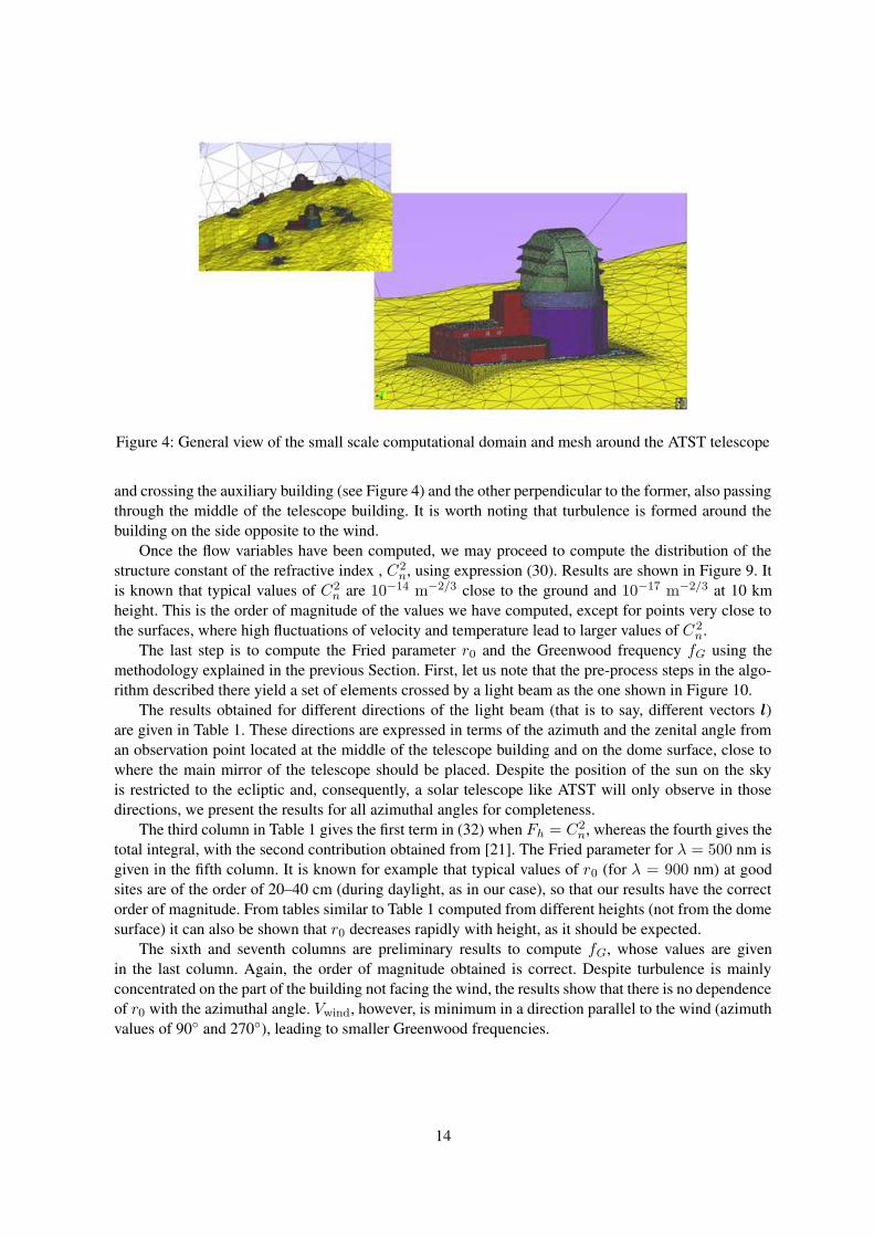
Figure 4: General view of the small scale computational domain and mesh around the ATST telescope

and crossing the auxiliary building (see Figure 4) and the other perpendicular to the former, also passingthrough the middle of the telescope building. It is worth noting that turbulence is formed around thebuilding on the side opposite to the wind.

Once the flow variables have been computed, we may proceed to compute the distribution of thestructure constant of the refractive index , C2

n, using expression (30). Results are shown in Figure 9. Itis known that typical values of C2

n are 10−14 m−2/3 close to the ground and 10−17 m−2/3 at 10 kmheight. This is the order of magnitude of the values we have computed, except for points very close tothe surfaces, where high fluctuations of velocity and temperature lead to larger values of C 2

n.The last step is to compute the Fried parameter r0 and the Greenwood frequency fG using the

methodology explained in the previous Section. First, let us note that the pre-process steps in the algo-rithm described there yield a set of elements crossed by a light beam as the one shown in Figure 10.

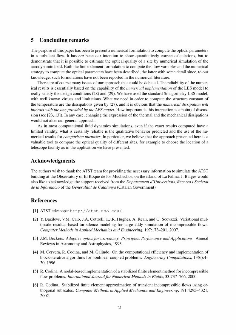
The results obtained for different directions of the light beam (that is to say, different vectors l)are given in Table 1. These directions are expressed in terms of the azimuth and the zenital angle froman observation point located at the middle of the telescope building and on the dome surface, close towhere the main mirror of the telescope should be placed. Despite the position of the sun on the skyis restricted to the ecliptic and, consequently, a solar telescope like ATST will only observe in thosedirections, we present the results for all azimuthal angles for completeness.

The third column in Table 1 gives the first term in (32) when Fh = C2n, whereas the fourth gives the

total integral, with the second contribution obtained from [21]. The Fried parameter for λ = 500 nm isgiven in the fifth column. It is known for example that typical values of r0 (for λ = 900 nm) at goodsites are of the order of 20–40 cm (during daylight, as in our case), so that our results have the correctorder of magnitude. From tables similar to Table 1 computed from different heights (not from the domesurface) it can also be shown that r0 decreases rapidly with height, as it should be expected.

The sixth and seventh columns are preliminary results to compute fG, whose values are givenin the last column. Again, the order of magnitude obtained is correct. Despite turbulence is mainlyconcentrated on the part of the building not facing the wind, the results show that there is no dependenceof r0 with the azimuthal angle. Vwind, however, is minimum in a direction parallel to the wind (azimuthvalues of 90 and 270), leading to smaller Greenwood frequencies.

14

Figure 5: Mean pressure contours along a longitudinal and a transverse cut

15

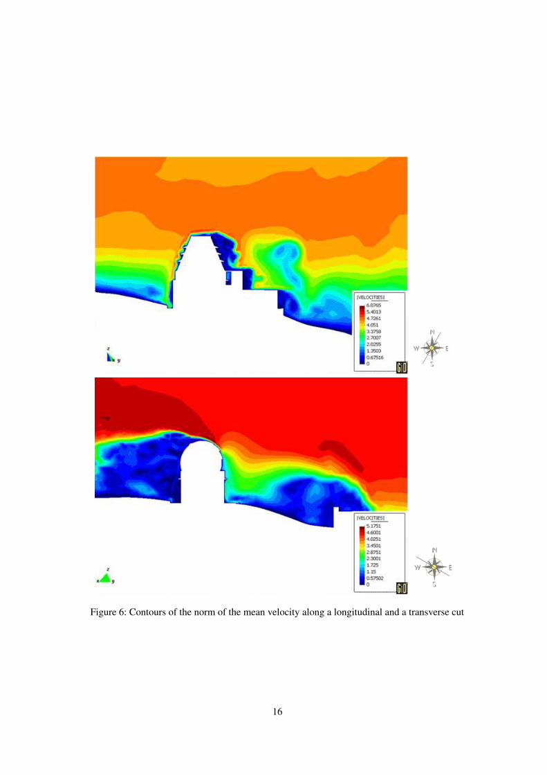
Figure 6: Contours of the norm of the mean velocity along a longitudinal and a transverse cut

16

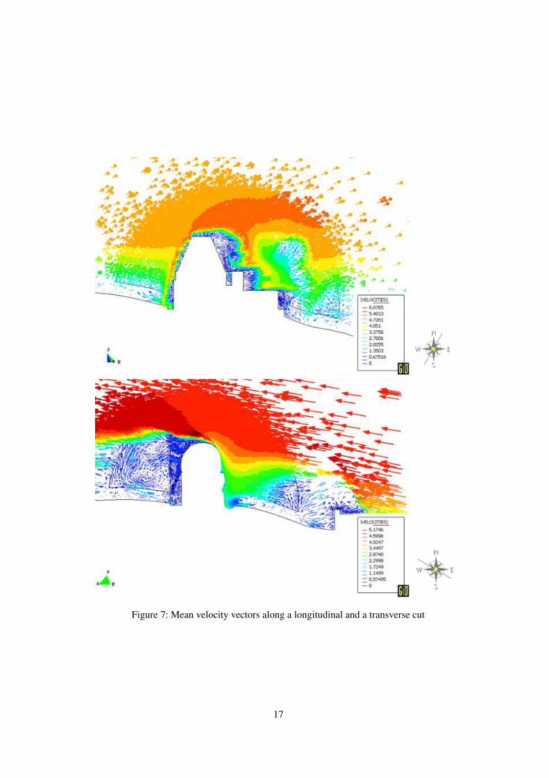
Figure 7: Mean velocity vectors along a longitudinal and a transverse cut

17

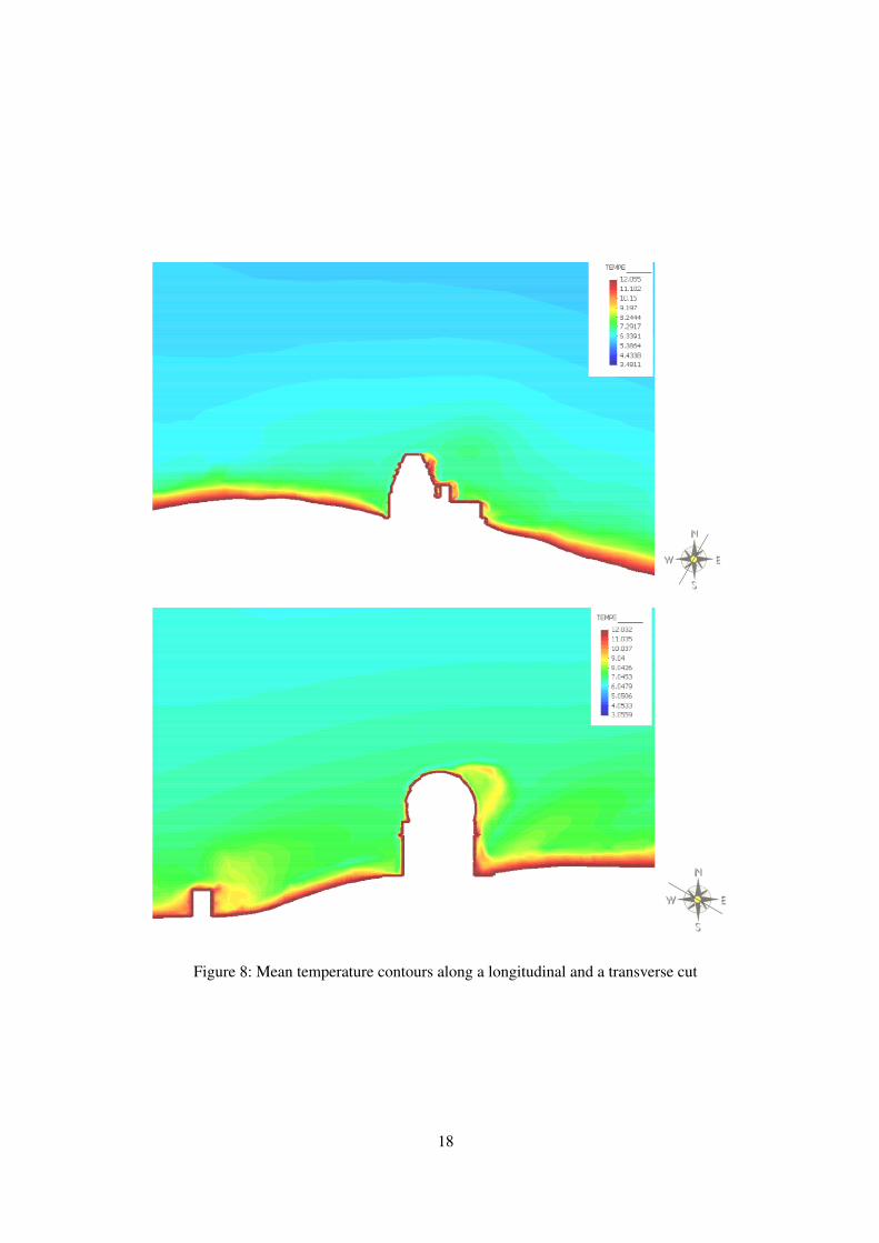
Figure 8: Mean temperature contours along a longitudinal and a transverse cut

18

Figure 9: Contours of C2n along a longitudinal and a transverse cut

19

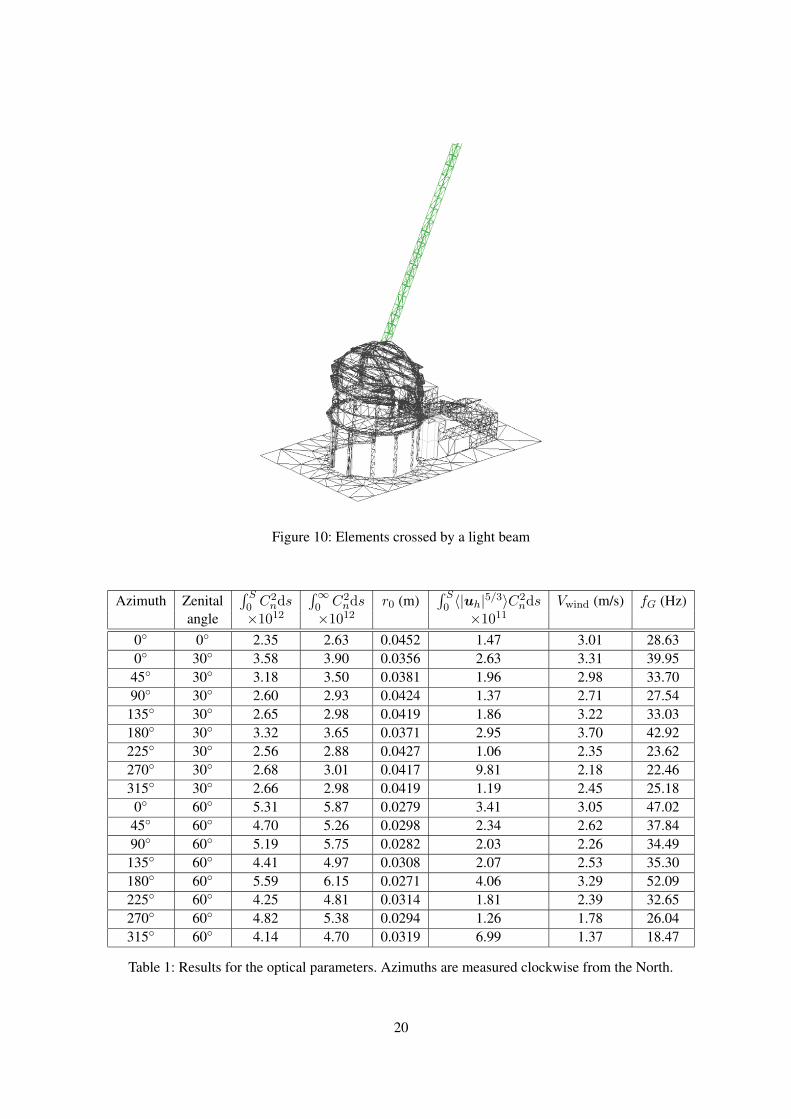
Figure 10: Elements crossed by a light beam

Azimuth Zenital∫ S0C2

nds∫

∞

0C2

nds r0 (m)∫ S0〈|uh|

5/3〉C2nds Vwind (m/s) fG (Hz)

angle ×1012 ×1012 ×1011

0 0 2.35 2.63 0.0452 1.47 3.01 28.630 30 3.58 3.90 0.0356 2.63 3.31 39.9545 30 3.18 3.50 0.0381 1.96 2.98 33.7090 30 2.60 2.93 0.0424 1.37 2.71 27.54135 30 2.65 2.98 0.0419 1.86 3.22 33.03180 30 3.32 3.65 0.0371 2.95 3.70 42.92225 30 2.56 2.88 0.0427 1.06 2.35 23.62270 30 2.68 3.01 0.0417 9.81 2.18 22.46315 30 2.66 2.98 0.0419 1.19 2.45 25.180 60 5.31 5.87 0.0279 3.41 3.05 47.0245 60 4.70 5.26 0.0298 2.34 2.62 37.8490 60 5.19 5.75 0.0282 2.03 2.26 34.49135 60 4.41 4.97 0.0308 2.07 2.53 35.30180 60 5.59 6.15 0.0271 4.06 3.29 52.09225 60 4.25 4.81 0.0314 1.81 2.39 32.65270 60 4.82 5.38 0.0294 1.26 1.78 26.04315 60 4.14 4.70 0.0319 6.99 1.37 18.47

Table 1: Results for the optical parameters. Azimuths are measured clockwise from the North.

20

5 Concluding remarks

The purpose of this paper has been to present a numerical formulation to compute the optical parametersin a turbulent flow. It has not been our intention to show quantitatively correct calculations, but todemonstrate that it is possible to estimate the optical quality of a site by numerical simulation of theaerodynamic field. Both the finite element formulation to compute the flow variables and the numericalstrategy to compute the optical parameters have been described, the latter with some detail since, to ourknowledge, such formulations have not been reported in the numerical literature.

There are of course many issues of our approach that could be debated. The reliability of the numer-ical results is essentially based on the capability of the numerical implementation of the LES model toreally satisfy the design conditions (28) and (29). We have used the standard Smagorinsky LES model,with well known virtues and limitations. What we need in order to compute the structure constant ofthe temperature are the dissipations given by (27), and it is obvious that the numerical dissipation willinteract with the one provided by the LES model. How important is this interaction is a point of discus-sion (see [23, 13]). In any case, changing the expression of the thermal and the mechanical dissipationswould not alter our general approach.

As in most computational fluid dynamics simulations, even if the exact results computed have alimited validity, what is certainly reliable is the qualitative behavior predicted and the use of the nu-merical results for comparison purposes. In particular, we believe that the approach presented here is avaluable tool to compare the optical quality of different sites, for example to choose the location of atelescope facility as in the application we have presented.

Acknowledgments

The authors wish to thank the ATST team for providing the necessary information to simulate the ATSTbuilding at the Observatory of El Roque de los Muchachos, on the island of La Palma. J. Baiges wouldalso like to acknowledge the support received from the Departament d’Universitats, Recerca i Societatde la Informacio of the Generalitat de Catalunya (Catalan Government)

References

[1] ATST telescope: http://atst.nso.edu/.

[2] Y. Bazilevs, V.M. Calo, J.A. Cottrell, T.J.R. Hughes, A. Reali, and G. Scovazzi. Variational mul-tiscale residual-based turbulence modeling for large eddy simulation of incompressible flows.Computer Methods in Applied Mechanics and Engineering, 197:173–201, 2007.

[3] J.M. Beckers. Adaptive optics for astronomy: Principles, Perfomance and Applications. AnnualReviews in Astronomy and Astrophysics, 1993.

[4] M. Cervera, R. Codina, and M. Galindo. On the computational efficiency and implementation ofblock-iterative algorithms for nonlinear coupled problems. Engineering Computations, 13(6):4–30, 1996.

[5] R. Codina. A nodal-based implementation of a stabilized finite element method for incompressibleflow problems. International Journal for Numerical Methods in Fluids, 33:737–766, 2000.

[6] R. Codina. Stabilized finite element approximation of transient incompressible flows using or-thogonal subscales. Computer Methods in Applied Mechanics and Engineering, 191:4295–4321,2002.

21

[7] R. Codina and A. Folch. A stabilized finite element predictor–corrector scheme for the incom-pressible Navier–Stokes equations using a nodal based implementation. International Journal forNumerical Methods in Fluids, 44:483–503, 2004.

[8] R. Codina, J. Principe, O. Guasch, and S. Badia. Time dependent subscales in the stabilizedfinite element approximation of incompressible flow problems. Computer Methods in AppliedMechanics and Engineering, 196:2413–2430, 2007.

[9] C.E. Colosqui and A.A. Oberai. Generalized Smagorinsky model in physical space. Computers& Fluids, 37:207–217, 2008.

[10] ELT project: http://www.eso.org/projects/e-elt/.

[11] L.P. Franca and S.L. Frey. Stabilized finite element methods: II. The incompressible Navier-Stokesequations. Computer Methods in Applied Mechanics and Engineering, 99:209–233, 1992.

[12] GTC telescope: http://www.gtc.iac.es/.

[13] O. Guasch and R. Codina. A heuristic argument for the sole use of numerical stabilization withno physical LES modelling in the simulation of incompressible turbulent flows. Submitted.

[14] R.J. Hill. Structure functions and spectra of scalar quantities in the inertial-convective and viscous-convective ranges of turbulence. Journal of the atmospheric sciences, 46:2245–2251, 1989.

[15] T.J.R. Hughes. Multiscale phenomena: Green’s function, the Dirichlet-to-Neumann formulation,subgrid scale models, bubbles and the origins of stabilized formulations. Computer Methods inApplied Mechanics and Engineering, 127:387–401, 1995.

[16] M.Z. Jacobson. Fundamentals of Atmospheric Modeling. Cambridge University Press, 2005.

[17] D.K. Lilly. The representation of small-scale turbulence theory in numerical simulation experi-ments. In H.H. Goldstine, editor, Proc. IBM Scientific Computing Symp. on Environmental Sci-ences, 1967.

[18] R. Lohner. Applied CFD Techniques. J. Wiley & Sons, 2001.

[19] L.J. Peltier and J.C. Wyngaard. Structure function parameters in the convective boundary layerfrom large eddy simulation. Journal of the atmospheric sciences, 52:3641–3660, 1995.

[20] S.B. Pope. Turbulent Flows. Cambridge University Press, 2000.

[21] C. Roddier and J. Vernin. Relative contribution of upper and lower atmosphere to integratedrefractive-index profiles. Applied optics, 16:2252–2256, 1977.

[22] F. Roddier. Adaptive optics in astronomy. Cambridge University Press, 2004.

[23] P. Sagaut. Large Eddy Simulation for Incompressible Flows. Scientific Computing, Springer,2001.

[24] V.I. Tatarski. Wave propagation in a turbulent medium. Dover Publications, INC, 1961.

[25] T.E. Tezduyar. Finite elements in fluids: Stabilized formulations and moving boundaries andinterfaces. Computers & Fluids, 36:191–206, 2007.

22

[26] P. Venkatakrishnan and S. Chatterjee. On the saturation of the refractive index structure function–I. Enhanced hopes for long baseline optical interferometry. Mon. Not. Royal Astronomical Society,224:265–269, 1987.

[27] L.P. Wang, S. Chen, and J.G. Brasseur. Examination of the hypothesis in the Kolmogorov refinedturbulence theory through high resolution simulations. Part 2. Passive scalar fields. Journal ofFluid Mechanics, 400:163–197, 1999.

23