a numerical investigation of wind speed effects on lake

A N U M E R I C A L I N V E S T I G A T I O N O F W I N D S P E E D E F F E C T S

O N L A K E - E F F E C T S T O R M S

P E T E R J. S O U S O U N I S ~

Penn State University, University Park, PA 16802, U.S.A.

(Received in final form 24 August, 1992)

Abstract. Observations of lake-effect storms that occur over the Great Lakes region during late autumn and winter indicate a high sensitivity to ambient wind speed and direction. In this paper, a two- dimensional version of the Penn State University/National Center for Atmospheric Research (PSU/ NCAR) model is used to investigate the wind speed effects on lake-effect snowstorms that occur over the Great Lakes region.

Theoretical initial conditions for stability, relative humidity, wind velocity, and lake/land temperature distribution are specified. Nine different experiments are performed using wind speeds of U = 0, 2, 4 , . . . , 16 m s -1. The perturbation wind, temperature, and moisture fields for each experiment after 36 h of simulation are compared.

It is determined that moderate (4-6m s -1) wind speeds result in maximum precipitation (snowfall) on the lee shore of the model lake. Weak wind speeds (0 ~< U < 4 m s 1) yield significantly higher snowfall amounts over the lake along with a spatially concentrated and intense response. Strong wind speeds (6 < U ~< 16 m s -1) yield very little, if any, significant snowfall, although significant increases in cloudiness, temperature, and perturbation wind speed occur hundreds of kilometers downwind from the lake.

1. Introduction

Lake-effect snow accounts for over one-half of the annual snowfall total in many lakeshore communities of the Great Lakes. A multitude of factors including local (coastal) geography, wind velocity, atmospheric stability, and lake-air temperature difference, combine to produce intense, small-scale storms that exhibit, at times, blizzard conditions across portions of the Great Lakes region. Remick (1942) described in some detail the development of such a storm near Lake Erie that occurred on October 18-19 1930. The heaviest snowfall, an incredible 48 inches (122 cm) occurred in Orchard Park, NY, which is approximately 24 km south of Buffalo, NY. In the city of Buffalo, only six inches (15 cm) were officially measured. Because that storm occurred in mid-October, the Lake Erie temperature (15 ~ and the prevailing air temperature (0 ~ did not result in an exceptionally large lake-air temperature difference (15 ~ Numerous citings exist in the litera- ture of lake-effect storms that developed from lake-air temperature differences greater than 15 ~ that have produced snowfall totals far less than 122 cm. Also, because most of the snow fell near the Lake Erie shore, orography was apparently not a primary forcing mechanism for that storm. Some other possible factors responsible for the heavy snow may have been the low-level stability, the vertical

1 Present Address: AOSS Department, The University of Michigan, Ann Arbor, MI 48109-2143, USA.

Boundary-Layer Meteorology 64: 261-290, 1993. �9 1993 Kluwer Academic Publishers. Printed in the Netherlands.

2 6 2 p . J . SOUSOUNIS

moisture distribution, and the prevailing wind velocity coupled with the lakeshore geometry. Remick (1942) in fact noted that one of the primary causes for the large snowfall total was the prevailing wind, which was force 5-6 (-12-14 m s -1) from the WSW, which was parallel to the long axis of Lake Erie.

The impact of the prevailing wind on wintertime lake-effect storms over the Great Lakes region has long been recognized. As early as the 1920's (e.g., Mitch- ell, 1921), the importance of the wind direction and thus the fetch was noted. Long feteches usually but not always result in the heaviest snowfalls. Short fetches may also produce significant snowfalls provided the lakeshore geometry enhances radial convergence and the nearby orography enhances lifting (Lavoie, 1972).

The wind direction determines not only which particular region receives the greatest snowfall and how much, but also the morphology of the storms. Kelly (1986) noted that the most frequently occurring storm type over Lake Michigan is that which exhibits multiple snow bands. He determined that when the wind direction was between WSW and NNW, multiple bands can develop 2-20 km apart and align themselves parallel to the wind. Hsu (1987) used both a linear analytic model and a nonlinear numerical model to study the effects of wind direction on lake-effect storms near Lake Michigan. His results indicated that three convergence centers develop near the eastern shore when a westerly wind prevails, two cells or snow bands develop when a northwesterly wind prevails, and a single midlake band develops when a northerly wind prevails.

Passarelli and Braham (1981) discussed the significance of a northerly wind across Lake Michigan for allowing strong, opposing land breezes to force an intense midlake snowband. Because of the shape of Lake Michigan, the north wind simulation away from the south shore is similar to a zero wind simulation during quiescent periods. The results obtained during the Lake Ontario Winter Storms (LOWS) project indicate similar findings (cf. Penc et al., 1991). For Lake Ontario, however, it is a westerly wind that yields a single midlake band, with northwesterly and southwesterly winds producing multiple bands. Recently, Hjelmfelt (1990) numerically simulated lake-effect storms near Lake Michigan for a variety of wind conditions. He was able to produce the four different types that Forbes and Merritt (1984) identified earlier. His study demonstrated the significant effects that atmospheric stability, lake-land surface roughness difference, lake-air temperature difference, wind direction and wind speed have on lake-effect storms. Regarding wind direction, he found that as the wind became more notherly and less westerly, the region(s) of convergence shifted away from the eastern shore of Lake Michigan towards the center of the Lake. His explanation was that the westerly component across the lake weakened so that equally strong land breezes developed to produce a midlake snowband for a northerly wind.

Niziol (1987) noted the importance of the vertical wind structure for determining lake-effect storm morphology near Lake Erie. Specifically, for a prevailing wind parallel to the long axis of the Lake, moderate directional shear (e.g., between 30 ~ and 60 ~ from the surface to 700 mb can cause multiple bands rather than a

W I N D S P E E D E F F E C T S ON L A K E - E F F E C T S T O R M S 263

single band. Stronger shear (e.g., greater than 60 ~ can lead to a breakdown of banded structure and just produce a stratocumulus deck with virtually no precipitation.

The wind direction and its vertical structure have significant effects on lake- effect storms. The wind speed also has significant effects. They were documented early by Rothrock (1969) who examined lake-effect storms in the vicinity of Lake Superior. He determined that a northerly geostrophic wind speed exceeding 5 m s 1 was required for significant lake-effect storms (e.g., >5 cm snow on the south shore within 24 hr) to develop. Lin (1989) examined analytically some of the inertial and frictional effects on airflow from an isolated circular surface-based heat source. He found that an in-phase relationship between heating and vertical motion exists for inviscid quasi-geostrophic (e.g., small Rossby number) flow. For a larger Rossby number flow, the advective effect of the flow dominates to produce a U-shaped response that results from upwardly propagating gravity waves. Sou- sounis and Shirer (1992) demonstrated analytically how the response to localized heating of a stable PBL with a strong inversion during a cold air outbreak situation can change markedly with wind speed. Yuen and Young (1986) also demonstrated analytically using a mixed-layer model how the PBL responds in different ways when thermally forced under strong and weak wind speeds.

The effects of wind velocity on other phenomena that are related dynamically to lake-effect storms have also been studied. Walsh (1974) determined theoretically the offshore wind speed that can prevent the development of a sea breeze. His results showed that strong offshore flows are required to prevent sea breezes when strong sea-land temperature differences exist. His results matched closely those obtained observationally by Briggs and Graves (1962). Arritt (1991) investigated sea breeze frontogenesis as a function of wind speed. He found that the maximum sea breeze perturbation exists when the background flow is slightly offshore (e.g., opposite to the sea breeze). Too strong an opposing offshore flow prevents a sea breeze from ever developing and an onshore background wind weakens the land- sea temperature gradient and hence the perturbation sea breeze.

Hayashi (1976), DeMaria (1985), and Raymond (1986) examined wind speed effects in the context of deep cumulus convection (e.g., latent heating). Raymond (1986) demonstrated analytically that the atmospheric responses to specified heating exhibit vertical motion maxima for a discrete set of wind speeds that are determined by the atmospheric stability and specified heating width (diameter). Bretherton (1988) noted that the transient thermal response of an inviscid fluid of Brunt-VfiisN~ frequency N and speed U confined between two parallel plates separated by a vertical distance H remains finite unless the Froude number NH/U is an integer multiple of ~-. Physick and Tapper (1990) examined the thermal response of the atmosphere to heating from The Salt Lake in Australia. They found the response to be much more localized and more intense for the case of zero background wind than for the case of nonzero background wind.

The above-mentioned studies provide strong evidence that the prevailing wind

264 P.J. sousouMs

plays a major role in the development and morphology of lake-effect storms. Much of that evidence has been derived empirically from observations or numerically from simulations of particular snow events. The studies do not, therefore, provide a sufficiently comprehensive theoretical explanation of how lake-effect storm characteristics depend on the prevailing wind. To develop a more fundamental understanding of how prevailing wind affects lake-effect storms, we have performed an idealized numerical study using analytic initial and boundary conditions based on actual observations. The study focuses specifically on the wind speed sensitivity of lake-effect storms. The knowledge obtained from this study along with that obtained from future idealized studies that will assess the effects resulting from other aspects of the prevailing wind (e.g., wind direction and vertical structure) will be used to assist our interpretations of more complicated and realistic case-study simulations of lake-effect storms to be performed later.

In this study we focus on the numerically simulated response of a theoretically initialized PBL that is heated by a warm, two-dimensional lake. We demonstrate the effects of a uniform background wind on the PBL response by examining the different responses for a series of mean wind speeds.

2. Model Description

We use a two-dimensional version of the Penn State University/National Center for Atmospheric Research (PSU/NCAR) numerical mesoscale model (MM4). This hydrostatic model uses a terrain-following sigma coordinate system. The momentum fields are computed on a grid that is staggered from the one on which all of the other variables are computed (e.g., Arakawa B grid). The finite difference routines are centered in space and in time. Additional model specifics are discussed in Anthes et al. (1987). We note that the two-dimensional version of MM4 is actually not a conventional two-dimensional model but rather a narrow slice of the three-dimensional version of MM4. The five gridpoint-wide slice allows only for diffusion in the cross-domain direction, and the model simulation is

observed on the middle (third) gridpoint of the slice.

2.1. MODEL DOMAIN CHARACTERISTICS

The model domain is oriented in the north-south direction and centered at 43.5 ~ N. A northerly basic state flow is specified. The flow direction and central latitude are both characteristic of lake-effect storms over the Great Lakes (e.g., Lakes Superior and Huron) . Because the Coriolis parameter changes weakly at mid- latitudes, the results from our study can be applied to other lake-effect storms despite the specified N - S orientation of the model. Hence, lake-effect storms that result from flows that are quasi-perpendicular to the long axes (e.g., westerly flow across Lake Michigan, northwesterly flow across Lakes Erie and Ontario, and northerly flow across Lakes Superior and Huron) may be examined with our model

domain.

WIND SPEED EFFECTS ON LAKE-EFFECT STORMS 265

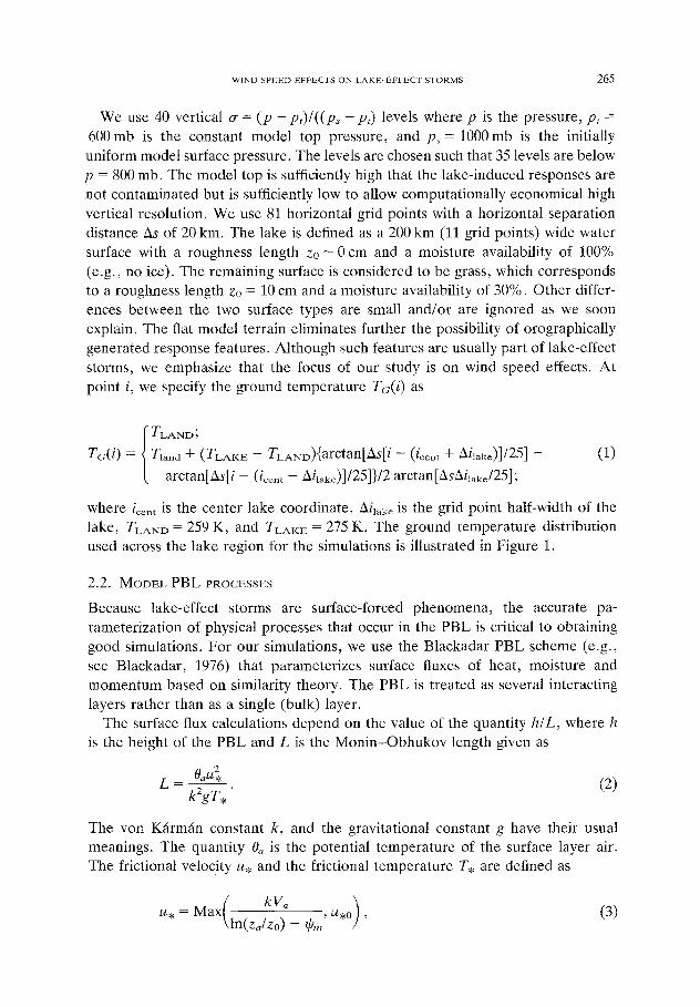
We use 40 vertical cr = ( p - P t ) / ( ( P s - Pt) levels where p is the pressure, Pt = 600rob is the constant model top pressure, and Ps = 1000mb is the initially uniform model surface pressure. The levels are chosen such that 35 levels are below p = 800 mb. The model top is sufficiently high that the lake-induced responses are not contaminated but is sufficiently low to allow computationally economical high vertical resolution. We use 81 horizontal grid points with a horizontal separation distance As of 20 kin. The lake is defined as a 200 km (11 grid points) wide water surface with a roughness length z 0 - 0 cm and a moisture availability of 100% (e.g., no ice). The remaining surface is considered to be grass, which corresponds to a roughness length Zo = 10 cm and a moisture availability of 30%. Other differences between the two surface types are small and/or are ignored as we soon explain. The flat model terrain eliminates further the possibility of orographically generated response features. Although such features are usually part of lake-effect storms, we emphasize that the focus of our study is on wind speed effects. At point i, we specify the ground temperature TG(i) as

f T L A N D ;

T G ( i ) = ~ Tland -~- ( T L A K E -- TLAND){arctan[As[ i - ( /cent d- Ahake)]/25] - [ arctan[As[i - ( / c e n t - - Ai~ak~)]/25]}/2 arctan[AsAi~akJ25];

(1)

w h e r e /cent is the center lake coordinate, A / l a k e is the grid point half-width of the l ake , TLAND = 259 K, and TLAKE = 275 K. The ground temperature distribution used across the lake region for the simulations is illustrated in Figure 1.

2.2. MODEL PBL PROCESSES

Because lake-effect storms are surface-forced phenomena, the accurate parameterization of physical processes that occur in the PBL is critical to obtaining good simulations. For our simulations, we use the Blackadar PBL scheme (e.g., see Blackadar, 1976) that parameterizes surface fluxes of heat, moisture and momentum based on similarity theory. The PBL is treated as several interacting layers rather than as a single (bulk) layer.

The surface flux calculations depend on the value of the quantity h / L , where h is the height of the PBL and L is the Monin -Obhukov length given as

(2) k Z g T , "

The yon Kfirmfin constant k, and the gravitational constant g have their usual meanings. The quantity 0a is the potential temperature of the surface layer air. The frictional velocity u , and the frictional temperature T, are defined as

= Max( k V , , U , o ) , b / , \ l n ( z J z o ) - ~,~ /

(3)

266 e.J. sovsotJNis

259 K

Fig. 1. Lake region, time-invariant ground temperature distribution (black curve) and initial vertical temperature profile (grey curve) used for the model simulations. Region 1, corresponding to the PBL with a value of NpBL = 1.0 • 10 .2 s -1, extends from the surface (1000 mb) to approximately 810 rob. Region 2, corresponding to the inversion with a value of N~Nv = 4.3 x 10 .2 s -l, extends from 810 mb (249 K) to 790mb (259 K). Region 3, corresponding to the troposphere with a value of NTno =

1.9 • 10-2s -1, extends from 790 to 600 mb.

T , = O~- Og , (4) ln(za/zo) - Oh

respect ively. The quant i ty Va is the wind speed in the surface layer; za is the height

of the lowest o-level; z0 is the roughness height; 0g is the potent ia l t e m p e r a t u r e at the ground; and U,o is a b a c k g r o u n d friction velocity. T h e nond imens iona l stabili ty

p a r a m e t e r s 4'm and Oh depend on the value for h / L and on the value of the surface-

layer bulk R icha rdson n u m b e r RiB, where

RiB - gz~ Ov~ - Ovg (5) 0~ v 2

The quant i t ies 0~a and Ovg are the vir tual potent ia l t e m p e r a t u r e s of the surface

layer and of the ground. D e p e n d i n g on the values for RiB and for h / L , the surface layer is classified at

each gr idpoint as e i ther (1) stable, (2) mechanica l ly dr iven turbulent , (3) forced convect ive , or (4) f reely convect ive . The prognos t ic equat ions for the mode l var iables in the P B L depend on whe the r the surface layer is s table to marginal ly uns table (classes 1 -3) or convect ive ly uns table (class 4). The stable (nocturnal) classes exist when RiB > 0, or when RiB < 0 and ]h/L I < 1.5. Fo r the noc turna l reg ime, the poten t ia l t e m p e r a t u r e 0a, the specific humidi ty qa, the nor the r ly wind ua, the wester ly wind va, and the liquid wa te r con ten t qc~ in the surface layer are

c o m p u t e d as

WIND SPEED EFFECTS ON L A K E - E F F E C T STORMS 267

Ot - - - -(H, -H~)/(OaC~Z,), (6a)

O q , _ (E~ - E , ) / ( p , z l ) , (6b) Ot

o u o = ( ~ , _ ~ , ~ ) / ( o o 2 1 ) , (6c) Ot

OVa = ( T l x - - Tsx)/(PaZl) , ( 6 d )

Ot

O q ~ _ C1/(Pazl ) . (6e) Ot

The quantity zl is the height of the lowest model layer; p~ and Cpm are the density of the surface layer air and the specific heat for moist air at constant pressure. The surface fluxes of sensible heat Hs, water vapor E,, and momentum % are given as

11, = - paCp,~ku, T , , (7)

E, = M p J - l ( q , g - qa ) , (8)

=- U 2 P~ * (ua, va) (9) ~'s(x,y) ~ a

The components u a and va correspond to the surface-layer southerly and westerly wind components. The quantity M is the moisture availability fraction; qgs and qa are the saturated specific humidity at the ground and the specific humidity of the surface layer, and

- -1

= k u , / l n | + - Oh (10) L \ K a

The quantity Ka = 2.4 x 10 -5 m 2 s -1 is a background value of molecular diffusivity. The subscript "1" in (6) indicates the fluxes of sensible heat HI, water vapor

E~, momentum ~'1, and condensation C1 at the top of level one. These fluxes are computed from K theory using

K = Ko + Sil 2Rc - Ri (11) Rc

The quantity K0 = 0.1 m 2 s -1 is a background diffusion value, Si is the surface- layer wind shear, Ri is the gradient Richardson number, and Rc is the critical Richardson number. The mixing length l is defined as

,V1/2 / . l = _,~ ~n (12)

268 P.J. SOUSOUN~S

The quantity Sm is a stability factor defined by Yamada (1983) and In is a neutral stability length scale defined as

In = kz[1 + (kz/lo)] -1 (13)

The quantity lo = 60 m is a constant mixing-length scale and z is the height above the surface. Above the surface layer, the prognostic variables are computed using

K theory. When the surface layer is convectively unstable (class 4), the model variables

in the surface layer at time ~-+ 1 are computed by

{FsZl Fs + ~ ) [ e x p ( hrn2xt t - ll+--FsAt (14) cG+i = c~- i + \h~mm hm Z l / h '

where o~ represents any prognostic variable, F1 and F, represent the corresponding fluxes at the top and at the bottom of the surface layer, h is the height of the PBL, and At is the time step. The mixing coefficient m is given by

h --1

m=Hi{paCpm(1 -e ) f [Ow-Ov(z ' )]dz '} , (15) Zl

in which �9 = 0.2 is the entrainment coefficient, and H1 is the sensible heat flux at the top of the surface layer given by the Priestley equation:

H1 = p a C p m Z i ( O v a - - O v l . 5 ) 3/2 X

" 2g " t/2 1 2 Z - 1/3 - 3 / 2

The subscript 1.5 refers to the middle of the second layer. Above the surface layer, the Eulerian time derivatives for the variables at a given model level are based on a mixing coefficient that decreases to zero at the top of the mixed layer and on the differences of the variables between the middle and the bottom of the

layer. Above the mixed layer, the prognostic variables are computed using K theory.

2 . 3 . M O D E L I N I T I A L A N D B O U N D A R Y C O N D I T I O N S

In order to focus on the effects of wind speed, we assume that the initial wind profile is directionally constant at a uniform wind speed U. Even without a lake- air temperature difference, some low-level model wind shear will develop as a result of mechanical mixing in the PBL. By not considering additional environmental shear, the effects of wind speed on the thermal response may be more easily

assessed. Most cold air masses prior to passing over the Great Lakes or other warm

bodies of water are characterized by some low-level marginal stability, a moderately strong cap or inversion at some height, and a moderately stable layer of air


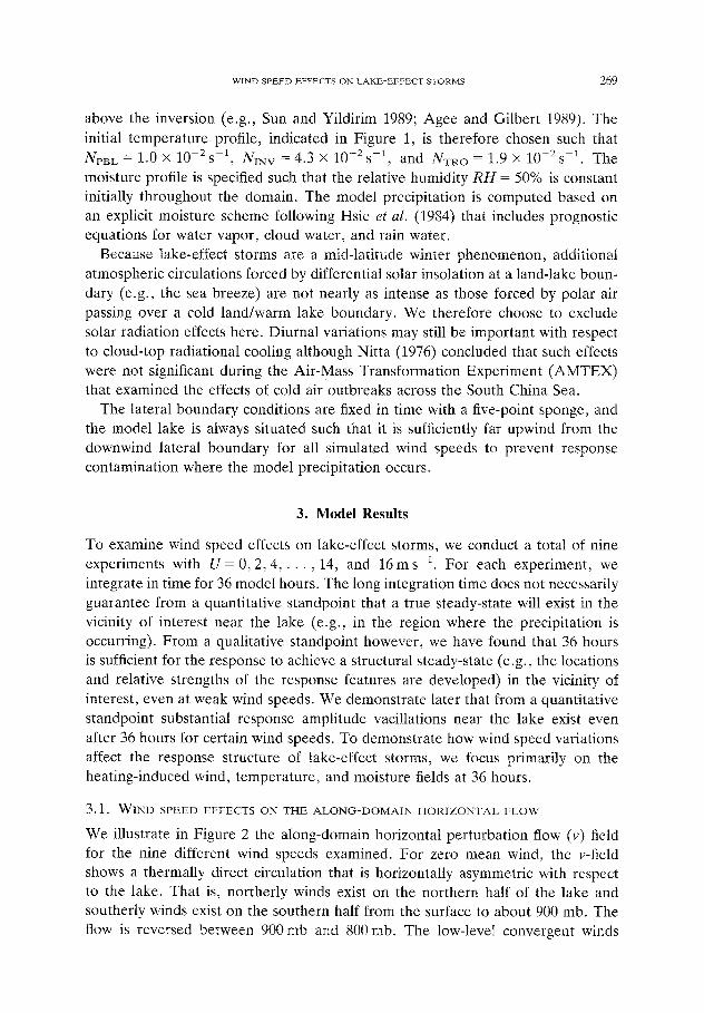
above the inversion (e.g., Sun and Yildirim 1989; Agee and Gilbert 1989). The

initial temperature profile, indicated in Figure 1, is therefore chosen such that NpBL = 1.0 X 10-2S -1, NINV=4.3 • 10-2S - I , and NTRO = 1.9 • 10-2S -1. The

moisture profile is specified such that the relative humidity R H = 50% is constant initially throughout the domain. The model precipitation is computed based on an explicit moisture scheme following Hsie et al. (1984) that includes prognostic equations for water vapor, cloud water, and rain water.

Because lake-effect storms are a mid-latitude winter phenomenon, additional atmospheric circulations forced by differential solar insolation at a land-lake boundary (e.g., the sea breeze) are not nearly as intense as those forced by polar air passing over a cold land/warm lake boundary. We therefore choose to exclude solar radiation effects here. Diurnal variations may still be important with respect to cloud-top radiational cooling although Nitta (1976) concluded that such effects were not significant during the Air-Mass Transformation Experiment (AMTEX) that examined the effects of cold air outbreaks across the South China Sea.

The lateral boundary conditions are fixed in time with a five-point sponge, and the model lake is always situated such that it is sufficiently far upwind from the downwind lateral boundary for all simulated wind speeds to prevent response contamination where the model precipitation occurs.

3. Model Results

To examine wind speed effects on lake-effect storms, we conduct a total of nine experiments with U = 0 , 2 , 4 , . . . , 14, and 1 6 m s -~. For each experiment, we integrate in time for 36 model hours. The long integration time does not necessarily guarantee from a quantitative standpoint that a true steady-state will exist in the vicinity of interest near the lake (e.g., in the region where the precipitation is occurring). From a qualitative standpoint however, we have found that 36 hours is sufficient for the response to achieve a structural steady-state (e.g., the locations and relative strengths of the response features are developed) in the vicinity of interest, even at weak wind speeds. We demonstrate later that from a quantitative standpoint substantial response amplitude vacillations near the lake exist even after 36 hours for certain wind speeds. To demonstrate how wind speed variations affect the response structure of lake-effect storms, we focus primarily on the heating-induced wind, temperature, and moisture fields at 36 hours.

3.1. WIND SPEED EFFECTS ON THE ALONG-DOMAIN HORIZONTAL FLOW

We illustrate in Figure 2 the along-domain horizontal perturbation flow (v) field for the nine different wind speeds examined. For zero mean wind, the v-field shows a thermally direct circulation that is horizontally asymmetric with respect to the lake. That is, northerly winds exist on the northern half of the lake and southerly winds exist on the southern half from the surface to about 900 rob. The flow is reversed between 900 mb and 800 mb. The low-level convergent winds

2 7 0 e. J, SOUSOUNIS

I C.

, > , ~ �9

~ o ~ ro

o

,zn " ~

�9 O , ,o ,.. ~

o . ~

�9 ~ o ~ r

�9 I : : ~ . O


indicate a maximum of nearly 4 m s - t , while the upper-level divergent winds indicate a max imum of nearly 7 m s -1.

For a mean wind speed of U = 2 m s -~, the lake-relative asymmetric pat tern no

longer exists. Additionally, the per turbat ion flow is extremely weak in the lowest 100 mb over the lake. Most of the response for this field is at higher levels. For

example, a northerly-southerly per turbat ion couplet with magnitudes less than 3 and 4 m s -1 respectively exists near 900 mb while a northerly per turbat ion maximum greater than 6 m s-1 exists at 800 rob. The background flow is 2 m s - l , and

so a flow reversal (e.g., a southerly flow component of - 4 m s -1) exists near the 800 mb level.

For the U = 4 m s i case in Figure 2, the v-field indicates that the flow increases

significantly (e.g., f rom 3 to 6 m s -1) near the ups t ream shore as a result of air passing from the cold (rough) land to the warm (smooth) lake. The downwind

half of the lake from the surface to 900 mb is characterized by horizontal convergence. A second divergence-convergence pat tern is present at low levels across

the next 200-300 km downwind. In the region from 900 to 800 rob, the strongest southerly flow speed is less than 4 m s -1 so that no flow reversal occurs; e.g., the wind everywhere has a northerly component . Finally, we note that significant response amplitudes (e.g., >2 m s-1) exist 200 km downwind from the lake.

The v-field for the response when U = 6 m s ~ is similar to that when U = 4 m s -1. An intense narrow band of convergence exists at the downwind shore. A southerly flow exists f rom near the surface to about 900 rob, but because

the magnitude is less than 6 m s -~, no flow reversal occurs. Significant response amplitudes exist 400 km downwind from the lake.

The results f rom the U = 8 through U = 16 m s -1 experiments indicate that the

basic v-field structure is preserved. The wavelength • of the downstream response increases particularly within the upper PBL from A = 500 km at U = 8 m s - t to

A = 900 km at U = 16 m s -1. These values compare well with those obtained using

the inertial oscillation wavelength 2~ i = 2~rU/f, where f is the Coriolis parameter . Along with an increasing wavelength, other notable changes in the v-field with increased wind speed include an increasingly deeper shear layer near the surface and a horizontally diffusing response ampli tude downwind. Significant response amplitudes extend as far as 1000 km from the lake when U = 16 m s -L. Directly

above the lake however, very little change in the basic state flow (e.g., v - 0) is evident.

3.2. WIND SPEED EFFECTS ON THE CROSS-DOMAIN HORIZONTAL FLOW

We illustrate in Figure 3 the cross-domain horizontal per turbat ion flow (u) field for the nine different wind speeds. For zero mean wind, the u-field shows low- level cyclonic flow centered over the lake with two concentric (two-dimensional) vortices of relatively intense (e,g., 4 m s 1 amplitude) winds. The inner vortex has a lateral extent (peak to peak) of approximately 75 km and the outer one has a lateral extent of approximately 400 kin. Above the concentric cyclonic vortices

2 7 2 e . J . SOUSOUNIS

~5.%-J.7 ; ~ _ " _ _ .

>5," 7 ;,~ '/. / IJ) l

!\. i i

\ J

B c~ ,

c~

7 m

o ~

~ o

e g

o ~

.go.=

O

~ 0

c-I

g

0

~q


near 800 mb, a substantially more intense anticyclonic vortex exists with maximum

winds of nearly 17 m s - t. For U = 2 m s -1, the response pat tern is basically the same as for the U = 0

case, except that near the surface only one (asymmetric) cyclonic vortex instead

of two is clearly defined. This surface vortex has a lateral extent of approximately 200 km with stronger cyclonic wind shear near the downwind shore. The anticyclonic vortex centered near 800 mb is also highly asymmetric. The peak westerly

wind greater than 16 m s -~ is directly over the upwind lakeshore while the peak easterly wind less than 11 m s -~ is 400 km farther downwind.

A narrow band of cyclonic wind shear near the surface at the downwind shore characterizes the response near the surface when U = 4 m s L. An upper-level anticyclonic vortex is still discernible although it is displaced downwind. The

westerly component is centered just lakeward of the downwind shore and the easterly component is centered 450 km farther downstream. Unlike the east-west upper level vortex components for the U = 2 m s 1 response, both components

for the U = 4 m s-~ response are almost equal in amplitude. For the U = 6 m s - t response, we see a significant change in the overall struc-

ture. The response at low levels is similar to that of the U = 4 m s -~ response

although it is somewhat more displaced and elongated in the direction of the wind. At upper levels, however, the response is markedly different. The singte anticyclonic (two-dimensional) vortices that were present for the U = 0, 2, and 4 m s -1 cases are now replaced by an oscillating pat tern that begins over the

lake and extends 700 km downwind. Westerly wind maxima are separated by an oscillation wavelength of approximately I = 500 kin.

The responses for the wind speeds U = 8 m s -~ through U = 16 m s -~ are qualitatively similar to that for U = 6 m s - t . The low-level features of these responses extend deeper into the PBL and become stronger as a result of increased mechan-

ical mixing and increased Coriolis forcing with increasing wind speed. Also, the oscillation wavelength increases monotonically and almost doubles from approxi-

m a t e l y A = 5 0 0 k m a t U = S m s ~ t o A = 1 0 0 0 k m a t U = 1 6 m s -~.

3.3. WIND SPEED EFFECTS ON THE TEMPERATURE FIELD

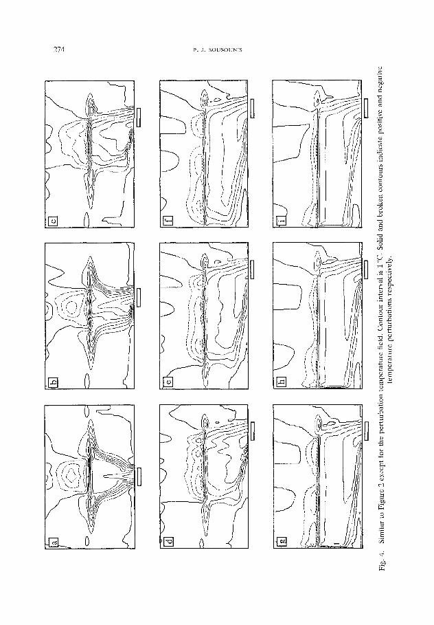
The wind speed effects on the per turbat ion tempera ture (t) field are illustrated in Figure 4. For the U = 0 case, a max imum tempera ture per turbat ion of over 8 ~ exists just above the surface at the center of the lake. Sharp horizontal tempera ture gradients flank the funnel-shaped perturbation. The per turbat ion is confined to the

horizontal extent of the lake at low levels but extends several hundred kilometers in either direction between 900-800 mb. The funnel shape is consistent with the v- field shown in Figure 2a. Low-level inflow concentrates the perturbat ion near the surface while upper-level outflow advects the heat away from the lake near the inversion (800 mb). Because of the specified strength of the inversion and because of the lake-air t empera ture difference for our simulations, the heat input from the lake into the a tmosphere is confined primarily to the lowest 200 mb.

2 7 4 p . J . SOUSOUNIS

',,_._. -,-,-,_

I " ,~i \ t ~,

<,

i' l ; ] ,

' \ \ k

~;i!')t~J~l ~ "'cJ

;7 " ~

rj,j i f

Vlili

X(~I

/ ,

i r \ \

I '

r ,

ii'

__:k

�9


The large negative temperature anomaly above 800 mb is a prominent feature

for all of the wind speed responses and can be explained easily. As the PBL is heated from below, the temperature of the air initially below the inversion increases. However , because of the original inversion strength, the potential temperature of the near-surface heated air is lower than that of the air initially above the inversion. As the heated air rises and lifts the inversion, the air cools adia- batically to a temperature less than that of the air initially above the inversion. The result is net cooling and destabilization of the air initially above the inversion.

For the U = 2 m s 1 case, the temperature perturbation tilts slightly downwind with height. As with the U = 0 m s -~ case, a maximum perturbation exceeding 8 ~ exists. The near-surface horizontal temperature gradient is over four times larger on the downwind lakeshore than it is on the upwind lakeshore. The cause for the stronger gradient downwind is enhanced convergence from opposing background and perturbation v-field flows. Above the lowest 25 rob, the relative magnitudes of the temperature gradients reverse as a result of the reversed along-domain flow.

The thermal response for the U = 4 m s -1 case indicates that the near-surface downwind lakeshore temperature gradient is stronger and the upwind lakeshore temperature gradient is weaker than those in the U = 2 m s - I case. At upper levels, the downwind temperature gradient weakens considerably while the upwind lakeshore temperature gradient remains essentially constant with height. The maximum temperature perturbation is slightly over 7 ~ at the downwind shore.

For the U = 6 m s -~ case shown in Figure 4d, the maximum temperature perturbation is only 6 ~ (for a lake-air temperature difference 2~T = 16 ~ Oscil- lations are quite apparent so that a secondary warming at the surface occurs from adiabatic motions nearly 200 km downwind from the lake (e.g., Figure 5d discussed in section 3.4). The half-length, which is the distance over which the perturbation amplitude drops by a factor of two, is nearly 600 km at 900 mb.

Further increases in wind speed lead to further decreases in the maximum temperature perturbation and increases in the half-length (so that it exceeds the domain width for U > 10 m s-A). The increases also lead to slightly weaker upwind temperature gradients and noticeably weaker downwind temperature gradients. Additionally, for speeds greater than U = 6 m s -~, oscillations are not as apparent as they are for the U = 6 m s 1case.

3.4. WIND SPEED EFFECTS ON THE VERTICAL MOTION FIELD

An important objective of our study is to understand how wind speed impacts the lake-effect storm precipitation distribution. It is therefore important to examine first in Figure 5 the vertical motion (w) field. For the U = 0 case, we see a region of intense (e.g., maximum amplitude of - 1 8 cm s - t ) ascent over the middle third of the lake extending from just above the surface to 800 mb. Above 800 mb, two significantly weaker regions of ascent flank the main ascent branch. Below 800 rob, descent with a maximum amplitude of nearly 3 cm s -1 exists on either side of the

2 7 6 P, J , S O U S O U N I S

C~

J ~ ' - '

<7 ....... >

~ B

D~ 8 r

8

_S

"5

7

.=. ~

o 8

e- �9

o

E ?

e-i

s

W i N D S P E E D E F F E C T S O N L A K E - E F F E C T S T O R M S 277

main ascent branch and extends outward with height from the surface to nearly

100 km on either side,

For a wind speed of U = 2 m s *, the lake-relative symmetry is noticeably

broken. A single region of intense ascent less than 100 km wide exists near the

downwind lakeshore. The maximum amplitude of approximately 7 cm s L is con-

siderably reduced from that of the U = 0 case. Significant descent exists in a

narrow area only on the upwind side of the ascent region. Downwind from the

lake, only very weak vertical motion is present.

A considerably different pattern is present when U = 4 m s -1. The upwind half

of the lake is characterized by descent (2 cm s - t ) while the downwind half of the

lake is characterized by comparably strong (4 cm s - t ) ascent. Beyond the down-

wind lakeshore, an oscillatory pattern is present. Specifically, another significant

(e.g., >2 cm s -~) ascent region exists nearly 200 km downwind from the lake. It

is interesting to note that of the three wind fields discussed, only the w-field

indicates a distinct oscillatory pattern at such a low U = 4 m s J wind speed.

Additionally, significant (e.g., Iw I > 1 cm s-5) perturbations in the vertical motion

field exist as far as 400 km downwind from the lake.

At U = 6 m s -1, we note a similar, but significantly enhanced, version of the

pattern obtained when U = 4 m s -1. Descending motion exists across the upwind

third of the lake. Although ascent exists across the downwind two-thirds of the

lake, a very narrow but intense (>8 cm s ~) region of primary ascent exists near

the lakeshore, An oscillatory pattern is present with a secondary region of signifi-

cant ascent located approximately 100 km farther downwind. The oscillating pat-

term decays much more quickly with distance from the lakeshore for the U =

6 m s- t case than it does for the U = 4 m s- 1 case. Significant response amplitudes

are confined to a 200 km area downwind from the lake.

We have seen thus far that an increase in wind speed has led generally to an

extension downstream of the response pattern. It is therefore interesting to note

that increasing the wind speed from U = 4 m s -~ to U = 6 m s -~ results in a retrac-

tion of the vertical motion response (e.g., the two significant ascent branches are

closer to the lake when U = 6 m s -~ than they are when U = 4 m s- l ) . Addition-

ally, the maximum response amplitude increases rather than decreases. The rea-

sons for such behavior will be discussed in section 4,

Comparing the U = 8 m s -1 pattern with the U = 6 m s -~ one, we see that the

descent is slightly weaker over the lake while the ascent is significantly weaker,

The only significant region of ascent for the U = 8 m s -~ response exists across a

greater horizontal area than does the primary ascent region for U = 6 m s -~. The

oscillatory pattern still exists, and it is considerably more extensive (e.g., the

wavelength for U = 6 m s 1 is approximately 200 km while that for U = 8 m s -~ is approximately 400 km).

Further increases in wind speed yield qualitatively similar response patterns to that obtained when U = 8 m s -1. The descent across the upwind part of the lake

intensifies gradually with increasing wind speed; exceeding 3 cms -1 when U =

2 7 8 p . J . s o u s o e N i s

10 m s -1 and exceeding 4 cm s 1 when U = 16 m s t. Additionally, the extent of the upwind lake descent is relatively independent of wind speed while the extent of the downwind lake ascent gradually extends farther downstream with increasing wind speed. The narrow regions of ascent near the upwind boundaries for the strong U > 8 m s ~ wind speeds are a result of the imposed lateral boundary

conditions but they do not affect the results in the regions of interest. Although we have not yet discussed the t ime-dependency of the responses, we

summarize in Figure 6 the wind speed and temporal dependencies of the maximum upward vertical motion amplitudes. The exact locations of these maxima are not shown, but because they are the strongest upward velocities, it may be understood

rather easily that for the entire 36 hour period they are located either somewhere

over the lake or just inland from the downwind lakeshore. For all but the strongest

wind speeds examined, Figure 6 indicates that peak ascent amplitudes occur 12 to 15 hours into each simulation. The simulations with wind speeds greater than U = 10 m s -1 have peak velocities occurring as early as 3 to 6 hours. Additionally, the

vertical mot ion amplitudes for the strong wind speed simulations (e.g., U/> 8 m s -~) decrease and then remain relatively constant with time after about 18 hours. The simulations for weak wind speeds (e.g., U ~ < 2 m s -~) indicate a sharp decrease in ascent amplitude with time late in the 36 hour period. For the wind speeds U = 4 m s -1 and 6 m -~, significant temporal oscillations of the maxi-

m u m ascent amplitudes occur. To summarize Figure 6, we note that the most intense ascent after 36 model

hours of integration occurs when U = 0 m s -~. The amplitudes then decrease with increasing wind speed between U = 0 and 4 m s -~. A second ascent peak occurs at U = 6 m s ~ before the ascent amplitudes decrease slowly with increasing wind speed. Figure 6 demonstrates how changes in wind speed can change fundament- ally the tempora l aspects of lake-effects storms. Although we do not actually show

the response fields as a function of time, we emphasize that the spatial aspects of the responses (e.g., qualitative aspects) near the lake remain much more constant

in t ime than do the amplitudes of the responses.

3.5. WIND SPEED EFFECTS ON THE MOISTURE FIELD

We now demonstra te how wind speed impacts the moisture distribution in lake- effect storms. We illustrate in Figure 7 the perturbat ion specific humidity (q) field. For a wind speed of U = 0, the greatest changes in specific humidity occur over the middle of the lake near the surface. Values of q > 1.5 g kg -1 exist over the central half and extend just above 900 rob. Less pronounced moistening occurs in the region between 900-800 mb although it extends 100 km past either lakeshore. The strong low-level increases in specific humidity are a result of moisture convergence occurring where values for q are initially relatively high. Far away from the lake, weak drying (e.g., q < 0) occurs because of subsidence. The drying is a result


f

i

/

/

/

/

,

0" <.

Fig. 6.

3o':

/

S

0

(3

S ,<

0 .~

15'

10!

Temporal variation (e.g., every 3 hours) of maximum vertical motion as a function of background wind speed.

of downward motion advecting sub-inversion air of lower specific humidity from

upper levels. The results for U = 2 and 4 m s -1 show a pat tern similar to that for U = 0.

Increasing areas of moistening that extend downwind past the lake along with slightly stronger (1.6 g kg -1) and weaker (1.3 g kg - I ) maximum perturbat ions respectively are notable features. At U = 6 m s 1, we see evidence of an oscillatory response in the q-field. Two areas of max imum moistening exist: one at the downwind lakeshore and one 200 km downwind from the lakeshore. We note that the two areas do not coincide with the two pr imary ascent branches shown in Figure 5d.

The specific humidity changes corresponding to the wind speeds U = 8 through 16 m s -1 indicate a downwind elongated region of moistening. Two maxima are no longer evident. The region of weak drying upwind also becomes less evident with increasing wind speed. At wind speeds above U = 10 m s 1, the q-field is contaminated to within 100 km of the lateral boundary.

2 8 0 P . J . s o u s o u N J s

@

[] 0

D

i -

~ D

[]

Io

,�89

iN

h J

�9 e ~

o

o

o , .o

[ 2 ]

I

i i

I

i i

i

o

0

,.r

r

c~

o

o

t<


3.6. W I N D S P E E D E F F E C T S O N T H E C L O U D F I E L D

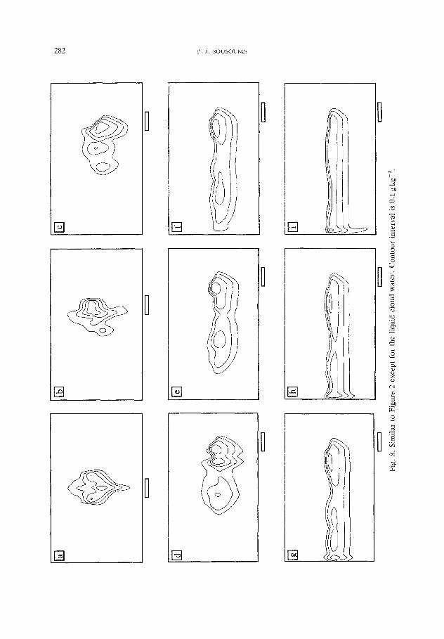
In Figure 8 we illustrate the cloud water (1) field responses for the nine wind

speeds. At U = 0, cloudiness (e.g., l < 0) extends 100 km on either side of the lake. The cloud base over the center of the lake is very low at 950 rob. It rises steeply at first and then more gradually to 800 mb near the edge of the cloudiness.

Peak cloud tops are also over the lake center near 700 rob. At U = 2 m s - I , we see a skewed version of the cloud pat tern for U = 0. A

sharp cloud water gradient exists on the upwind edge that is colocated with the upwind lakeshore. The cloud water maximum is located over the downwind

lakeshore and another weaker maximum is located 200 km farther downstream.

Both maxima are in regions of relatively low cloud base.

At U = 4 m s -1, the cloudiness pat tern is reminiscent of a plume that is generated by the heat and moisture f rom the lake. The cloud edge is about 20 km (e.g., 1 grid point) lakeward of the upwind lakeshore. The cloud base drops sharply f rom 850 nab at the edge to 960 mb over the downwind half of the lake

and rises sharply for a short distance past the lake. Maximum cloud depth occurs over the downwind edge. Three cloud water maxima are evident downwind and spaced approximately 200 km apart. At U = 6 m s - l , three cloud water maxima also exist. One is at the downwind lakeshore, an almost equally strong one is 100 km downwind, and a third weaker one is 500 km farther downwind. For both the

U - - 4 and U = 6 m s -1 fields, the cloud water maxima are co-located with the

ascent maxima indicated in Figs. 5c and d. At U = 8 m s - l , we note a significantly more shallow cloud pattern with maxi-

m u m cloud depths only slightly greater than l k m . (For weaker wind speeds, maximum cloud depths are approximately 2 km.) Two cloud water maxima are present. The pr imary max imum is again over the downwind lake edge while a

second weaker maximum is nearly 600 km farther downwind. The cloud pat terns for the stronger wind speeds are similar to that for U = 8 m s - ~. At U = 16 m s-~, almost the entire upwind half of the lake (4-5 grid points) is cloud-free. These results compare favorably with satellite photographs of land-lake (cf. Figure 1 of

Kelly, 1982) or land-ocean (cf. Figure 1 of Grossman and Betts, 1990) boundaries taken during cold air outbreaks associated with strong winds. The photographs

indicate significantly large clear-air regions in excess of 50 km. The results also compare favorably with those from Sun and Hsu (1988) who simulated numerically a cold air outbreak across the South China Sea. The results f rom their simulations demonstra ted that cloudiness can extend for distances greater than 1000 km from shore, although the much larger extent of an ocean relative to our small lake is a fundamental difference between their study and ours. We note finally that the obvious contaminat ion of the cloud water distribution near the lateral boundary for wind speeds greater than U = 10 m s 1 does not affect our results near the lake.

282 e . J . SOUSOUN[S

[]

[]

[]

[]

[]

[]

[]

[]

I

7

r

�9

�9

B~ �9

-d

B~


Fig. 9.

30 300

2s 2s0

2o 2oo

lS lS0 o

L, 10 100 o

5 50

0

u "100 8 " DiStance from Lake Center WindsPeeCl (~s) (kin)

L a k e - r e l a t i v e snowfa l l to ta l s a f t e r 36 h o u r s as a f u n c t i o n o f w i n d speed . S n o w f a l l to ta l s b a s e d

o n a 20 : 1 so l id : l iquid ra t io .

3.7. WIND SPEED EFFECTS ON THE PRECIPITATION DISTRIBUTION

In F igu re 9 we i l lus t ra te the 36-hour to ta l l ake - r e l a t i ve p rec ip i t a t i on d i s t r ibu t ion

for the var ious wind speeds . F o r all of the m o d e l s imula t ions , all of the prec ip i -

t a t ion falls as snow, a l though the m o d e l ou tpu t is ca lcu la ted as l iquid p rec ip i t a t ion .

Thus , in o r d e r to d i sp lay snowfal l to ta ls , we use a snowfal l : l iquid wa te r ra t io o f

20 :1 that is typica l of l ake-e f fec t snowstorms . In F igure 9, we see tha t the maxi-

m u m snowfal l amoun t s d r o p a lmos t exponen t i a l l y , and tha t the aer ia l cove rage of

the snow t rans la tes d o w n w i n d with increas ing wind speed . W h e n U = 0 m s 1, the

m a x i m u m snowfal l of 270 m m occurs ove r the cen t ra l po r t i on of the lake . No

snowfal l occurs ove r l and on e i the r side of the lake. W h e n U = 2 m s -1, mos t of

the snow occurs ove r the l ake a l though the d o w n w i n d l a k e s h o r e rece ives abou t

6.2 m m of snow. A m a x i m u m snowfal l of 60 m m at the downwind l a k e s h o r e occurs

at U = 4 m s - 1. W h e n U = 6 m s - 1, the l a k e s h o r e rece ives less than 1 m m of snow.

Mos t of the m e a s u r a b l e snow occurs d o w n w i n d f rom the l ake with a m a x i m u m of

17 m m occur r ing 60 km f rom the shore . W h e n U = 8 m s 1, the snowfal l d i s t r ibu-

t ion is such tha t a lmos t no snow has fa l len for a 100 km-w ide reg ion d i rec t ly

2 8 4 P . J . SOUSOUN~S

adjacent to the downwind lakeshore. Finally, for wind speeds U >~ 10 m s t, no measurable snow is produced in the model simulations.

We note that the lack of snowfall at strong wind speeds in our simulations may not be consistent with observations. The study by Remick (1942) discussed earlier, where winds were approximately 12 m s 1 and where snowfall totals were as great as 48 inches (122 cm), is one such observed example. However, we stress that other factors such as orography and lake geometry, which we do not address in our study, are present for actual lake-effect storms. Hjelmfelt (1992) noted recently how the presence of orography enhances the vertical motion (and hence the precipitation rate) in proportion to the mean wind speed and to the slope of the orography. The presence of positive curvature (e.g., the center of lakeshore curvature is upwind) can also act as an atmospheric lens to focus more radially the horizontal flow, increase convergence, and enhance vertical motion and precipitation. It is quite possible that for sufficiently upwardly sloping terrain, snowfall amounts at the downwind lakeshore can increase continuously with increasing wind speed when the flow is parallel to the long axis of an elliptically shaped lake.

4. Discussion

Our analyses of the wind, temperature, moisture and precipitation fields indicate that the most intense responses for each field occur primarily when U = 0. Gen- erally, an increase in wind speed tends to weaken and broaden extensively the responses. Figures 2-5 and Figures 7 -9 demonstrate the large-scale impacts that lake-induced heating can have on the atmosphere during cold air outbreaks associated with strong winds. Despite the fact that snowfall may be limited to distances less than 100km from the downwind lakeshore, significant increases in wind, temperature, humidity, and cloudiness may occur in regions that are several hundred kilometers downwind from a lake. While snowbelt communities such as Erie, PA, Buffalo, NY, and Cleveland, OH can receive considerable lake-effect snows during the winter, the other above-mentioned effects have long been recognized by residents in places such as Harrisburg, PA, Detroit , MI, and other areas that are several hundred kilometers downwind (e.g., south or east) from the nearest Great Lake.

We summarize in Table I how the maximum amplitudes of the perturbation features for each field at 36h change with wind speed. For those wind speeds where the response is either contaminated obviously near the lateral boundaries or where the maximum amplitude feature is very far downwind from the lake, we consider the amplitudes of the near-lake features. Additionally, we have subdiv- ided in Table I several of the fields examined earlier to distinguish northerly from southerly, easterly from westerly, and ascending from descending motions. Table I indicates that, with a few noted exceptions, all fields show a decrease in amplitude with increasing wind speed. The maximum northerly (N) perturbation occurs at U = 16m s - t and it is apparently more a result of mechanical forces such as


TABLE I

Maximum response amplitudes at 36h for northerly perturbation flow (N) in m s -/, southerly perturbation flow (S) in m s 1 westerly perturbation flow (W) in m s ~ easterly perturbation flow (E) in m s -1, ascent (A) in cm s 1, descent (D) in cm s 1, perturbation temperature (T) in ~ perturbation moisture (O) in gkg L cloud water (L) in gkg -1, and total snowfall (P) in ram. Total snowfall is

obtained by summing the amounts at each gridpoint.

U N S W E A D T Q L P

0 6.59 7.19 17.36 1 7 . 4 9 19.33 3.86 9.21 1.69 0.47 516.92 2 6.81 3.83 16.80 10.89 7.98 4.35 9.20 1.70 0.51 363.22 4 3.89 3.60 11.68 9.37 4.88 4.42 8.08 1.41 0.44 191.48 6 4.76 3.34 8.49 8.85 9.72 7.09 6.94 1.27 0.53 61.02 8 4.23 3.62 7.26 8.13 4.31 3.08 6.57 1.02 0.52 9.35

i0 4.57 3.56 5.73 2.55 4.15 3.67 6.13 0.90 0.49 0.00 i2 5.33 3.76 4.92 2.55 3.21 4.26 6.21 0.83 0.46 0.00 i4 6.21 3.92 5.37 2.41 3.58 4.73 6.16 0.78 0.43 0.00 i6 7.00 3.53 6.21 2.20 4.12 4.64 6.18 0.77 0.41 0.00

m o m e n t u m mixing wi thin the P B L than it is a resul t of l ake i nduc e d hea t ing . The

m a x i m u m sou the r ly p e r t u r b a t i o n (S) r ema ins re la t ive ly cons tan t wi th changes in

wind s p e e d af te r w e a k e n i n g m a r k e d l y f rom a m a x i m u m at U = 0 m s -1. The

m a x i m u m wes te r ly (W) and eas te r ly (E) p e r t u r b a t i o n s in Tab le I ind ica te a gene ra l

dec rea se in a m p l i t u d e with increas ing wind speed . I t is in te res t ing to no te tha t

increases in the m a x i m u m wes te r ly p e r t u r b a t i o n occur for inc reases in wind speed

a b o v e U = 12 m s 1. Such increases are r e l a t e d again a p p a r e n t l y to mechan ica l

(e .g . , Cor io l i s forcing) r a the r than to t h e r m a l forcing. A second n o t e w o r t h y fea tu re

is the d is t inct w e a k e n i n g of the m a x i m u m eas te r ly p e r t u r b a t i o n as wind s p e e d

increases f rom U = 8 to U = 10 m s - L F o r the ver t ica l mo t ions , we no te tha t the

mos t in tense descend ing (D) m o t i o n as well as the second mos t in tense ascend ing

(A) m o t i o n occur at U = 6 m s *. Because the mos t in tense descen t occurs at the

upwind l ake sho re , the increases in a m p l i t u d e for the descend ing m o t i o n for in-

c reases in wind speed a b o v e U = 12 m s - I a re once again mos t l ike ly a resul t of

mechan i ca l r a the r than t he rma l forc ing (e .g . , changes in surface roughness ) . The

m a x i m u m t e m p e r a t u r e (T) p e r t u r b a t i o n s and the specific humid i ty (Q) per -

t u rba t i ons dec rea se a lmos t s tead i ly wi th increases in wind speed . T h e m a x i m u m

in l iquid c loud wa te r (L) occurs no t at U = 0 m s -1 bu t at U = 6 m s -1. F ina l ly ,

we no te the a lmos t e x p o n e n t i a l dec l ine of to ta l snowfal l (P) wi th increases in wind

speed .

O u r analyses suggest tha t severa l d i f fe ren t types of l ake-e f fec t s to rms m a y be

poss ib le , d e p e n d i n g on b a c k g r o u n d wind speed . The resul ts ind ica te tha t significant

changes in the gene ra l r e sponse p a t t e r n for l ake-e f fec t s torms m a y occur when

the b a c k g r o u n d wind speed increases pas t a t h r e sho ld va lue . In our s imula t ions ,

such changes occur when wind speed increases f rom U < 4 m s i to U > 6 m s-~.

The weak wind s p e e d (0 m s 1 ~< U ~< 2 m s -1) m o d e l r e sponses are each charac-

t e r i zed by a single in tense ascent m a x i m u m (cf. F igu re 5) and e x t r e m e l y w e a k or

286 e.J. SOUSOUNIS

nonexistent signatures at distances greater than 200 km from the lake. As the wind

speed increases f rom U = 0 to U = 4 m s ~, both the ascent maximum and the precipitation distribution shift downwind, broaden in extent, and decrease in

amplitude. The model responses for strong wind speeds ( 8 m s - l ~ < U < 1 6 m s -1) are

characterized by oscillatory patterns that are significantly less pronounced near the lake than those for U = 4 and 6 m s - i in that only a single region of significant ascent exists. Also, virtually no snowfall occurs for these wind speeds. Because, however, the oscillatory patterns elongate downwind as the wind speed increases f rom U = 8 to U 16 m s - i significant increases in cloudiness, moisture, tempera-

ture, and winds exist hundreds of kilometers downwind from the lake. The model responses at U = 4 and U = 6 m s t appear significantly different

f rom either the weak wind speed or the strong wind speed responses. For example, two very intense ascent maxima develop downwind from the downwind lakeshore

at U = 4 m s -1. One maximum is located just inland from the shore while the other is 200 km farther downwind. Also, the highest snowfall amounts occur

downwind f rom the lake for these two wind speeds. The responses are unique also from a temporal perspective. Recalling Figure 6, we may note the very large temporal oscillations of the magnitudes for the pr imary ascent branches. Neither the weak nor the strong wind speed responses exhibits such large amplitude oscillations. Such large-amplitude temporal oscillations are characteristic of many

dynamical systems that are near resonance. A partial explanation of why such unique behavior occurs for the U = 6 m s -

response can be provided by Sousounis and Shirer (1992). In their linear analytic

study of cold air outbreaks, a Froude number Fr dependence on thermally forced steady-state responses was found to exist for cold PBLs flowing across warm lakes.

Their Froude number Fr was defined in terms of a mean wind speed U, a mean PBL depth H, and a mean Brunt-V~iis~il~i frequency N. Specifically, for Fr = r r U / N H < 1, a non-oscillatory (subcritical) response was found to exist. For Fr > 1, an oscillatory (supercritical) response was found. For Fr = 1, a resonance (critical) type of response was found that was characterized by extremely large

amplitudes and relatively small spatial extent. Heuristically, if we consider that the Froude number is a ratio of mean wind

speed U to gravity wave speed cg = NH/rr , then we see that a Froude number Fr = 1 indicates that U = cg. The gravity wave speed is the speed with which thermally excited waves propagate horizontally both upwind and downwind from the lake. When Fr < 1 and U < %, thermal excitations can propagate in either

direction. When Fr > 1 and U > cg, thermal excitations can propagate only downwind. When Fr = 1 and U = cg, however, thermally excited waves at the downwind lakeshore are prevented from propagating upwind and energy is therefore concentrated in a narrow region near the lakeshore.

For all of our simulations, we have used a thermal stratification within the PBL characterized by a Brunt-Vfiisfil~i frequency of N = 1.00 • 10-2S 1 and a PBL

WIND S P E E D EFFECTS ON L A K E - E F F E C T STORMS 287

depth (measured fl'om the surface to the base of the inversion) of H = 2 km. Using the above definition for Fr, and the above values for N and H, we see that a value of Fr = 1 corresponds to a wind speed of U = 6 .37ms-* . Despite significant differences between our numerical model and their linear analytic model (e.g., lack of a true rigid lid), our response at U = 6 m s -1 may nonetheless be the nonlinear temporal version of their linear steady analytic critical (Fr = 1) response. Our weak and strong wind speed responses may furthermore be evidence of their subcritical and supercritical response types.

A comparison of snowfall totals produced by the model with observed lake- effect snowfall totals may indicate a "dry" bias of the model. As we have previously mentioned, one such explanation could be the intentionally omitted orography from the model. A second possible explanation could be that the model grid spacing was not sufficiently small to represent more capably small-scale cumulus convection. A third possible explanation may be that numerically modeled lake- effect storms may be highly sensitive to the cumulus parameterization scheme used. For our simulations, we have used an explicit moisture scheme. The scheme is suitable for lake-effect precipitation that falls as rain as opposed to snow in terms of parameterized accretion rates and terminal fall speeds for example. We intend to address the sensitivity of our results to changes in grid resolution and convective parameterization schemes in subsequent studies. Because the results compare favorably with those from a linear analytic model, the underlying dyna- mics seem to be substantially linear and so we do not expect to see significant differences in the results from our subsequent studies.

The scientific interest that lake-effect storms generate for meteorologists may be closely motivated by the interest that they generate for the general public residing in many lakeshore communities. The societal impacts of lake-effect storms are more difficult to assess from our study because certain aspects of the weather (e.g., visibility) can not be addressed easily with the model used. Thus, it is rather difficult to determine, for example, which wind speed would produce the poorest visibility and/or the most hazardous driving conditions during a lake-effect storm. We have seen that although weak background winds produce intense responses, much of the snow is over the water and the visibility in nearby lakeshore communities may remain reasonably good. Moderate wind speeds ( 4 - 6 m s -1) produce weaker snowfall rates that are concentrated near the lakeshore although the strongest perturbation winds associated with the response are not co-located with the heaviest snow. Lake-effect storms that develop during wind speeds in excess of 10m s -* may lead to very poor visibility despite lighter snowfall rates and weaker perturbation winds because of the stronger background wind speed.

Factors such as visibility, precipitation type, and snowdrift potential are important aspects of winter storms and they are difficult to assess quantitatively with current numerical weather prediction models. Such factors are even more difficult to assess regarding lake-effect storms because of their intense nature and small size. Our model results can give a good understanding of how wind speed can

288 P. J , S O U S O U N I S

influence certain meteorological aspects of lake-effect storms but they can only suggest how wind speed may influence other aspects of these storms. Such aspects are beyond the scope of our current study and may be more unfortunately beyond the capabilities of current numerical models.

5. Summary and Conclusions

We have used the P S U / N C A R mesoscale model in a two-dimensional mode to examine the effects of wind speed on lake-effect storms. The model lake was parameterized as a 200 km wide water surface of specified temperature distribution. The terrain on either side was flat and approximately 15 ~ cooler than the lake. The initial atmospheric stability within the model domain was specified as a function of the vertical coordinate o" = ( p - P t ) / ( P s - P t ) .

We conducted nine experiments corresponding to U = 0, 2, 4, 6 , . . . , 1 6 m s -1, and then we compared the 36-hour wind, temperature and moisture fields. The results indicated relatively intense and localized responses for all fields for weak wind speeds (0 m s -1 <~ U ~< 4 m s- i ) . The response intensity and lake-relative symmetry of the responses both diminished with wind speed increasing from U = 0 to U = 4 m s -~. For the weak wind speed range, snowfall totals diminished although the amount of snow received at the downwind lakeshore increased.

The response for U = 6 m s -1 appeared significantly different than those for lower wind speeds. Specifically, an oscillatory pattern was evident and the response was fur thermore characterized by two relatively intense regions of ascent downwind from the lake.

The responses at stronger (e.g., U > 6 ms -1) wind speeds were also of an oscillatory nature. Specific differences included a more horizontally elongated and weaker response. Also, only one significant region of ascent centered on the downwind lakeshore was evident for the strong wind speed responses. Significant increases in cloudiness, temperature and winds were evident as far away as 1000 kin.

We conclude that background wind speed plays a significant role in lake-effect storms. Specifically, there exists a wind speed for which snowfall is maximized at the downwind lakeshore. For our particular set of initial conditions, the wind speed for maximum lakeshore snow yields a Froude number very close to unity. The maximization of lakeshore snowfall is a combined result of advecting downwind the entire region where snow can fall and dynamically tuning the thermally induced response to near-resonance. We end our study by noting that the Froude number Fr may be a useful parameter to examine concerning the forecasting of

lake-effect storms.

Acknowledgments

This research was performed while the author satisfied a Post-Doctoral appoint- ment at Penn State University that was supported under Grant ATM 87-22512.

WIND S P E E D EFFECTS ON L A K E - E F F E C T STORMS 289

Computing support for the numerical model simulations was provided by the Scientific Computing Division at the National Center for Atmospheric Research. Support for figure drafting, manuscript writing and publication was provided by research funds from the Atmospheric, Oceanic and Space Science Department at the University of Michigan.

References

Agee, E. M. and Gilbert, S. R.: 1989, 'An Aircraft Investigation of Mesoscale Convection over Lake Michigan During the 10 January 1984 Cold Air Outbreak', J. Atrnos. Sci. 46, 1877-1897.

Anthes, R. A., Hsie, E.-Y. and Kuo, Y.-H.: 1987, 'Description of the Penn State/NCAR Mesoscale Model Version 4 (MM4)', NCAR Technical note NCAR/TN-282+STR, 66 pp.

Arritt, R. W. : 1991, 'A Numerical Study of Sea Breeze Frontogenesis', Fifth Conference on Meteorology and Oceanography of the Coastal Zone, 26-29, Miami, 1991.

Blackadar, A. K.: 1976, 'High Resolution Models of the Planetary Boundary Layer', in Pfafflin and Ziegler (eds), Advances in Environmental Science and Engineering 1, Gordon and Breach, New York, pp. 50-85.

Bretherton, C. S.: 1988, 'Group Velocity and Linear Response of Stratified Fluids to Internal Heat or Mass Sources', J. Atmos. Sci. 45, 81-93.

Briggs, W. G. and Graves, M. E.: i962, 'A Lake Breeze Index', J. Appl. Meteorol 23, 939-949. Danard, M. B. and Rao, G. V.: 1972, 'Numerical Study of the Effects of the Great Lakes on a Winter

Cyclone', Mon. Wea. Rev. 100, 374-382. DeMaria, M.: 1985, 'Linear Response of a Stratified Tropical Atmosphere to Convective Forcing', J.

Atmos. Sci. 42, 1944-1959. Forbes, G. S. and Merritt, J. M.: 1984, 'Mesoscale Vortices over the Great Lakes in Wintertime',

Mon. Wea. Rev. 112, 377-381. Grossman, R. L. and Betts, A. K.: 1990, 'Air-Sea Interaction During an Extreme Cold Air Outbreak

from the Eastern Coast of the United States', Mon. Wea. Rev. 118, 324-342. Hayashi, Y.: 1976, 'Non-Singular Resonance of Equatorial Waves Under the Radiation Condition', J.

Atmos. Sci. 33, 183-201. Hsie, E.-Y., Anthes, R. A. and Keyser, D.: 1984, 'Numerical Simulation of Frontogenesis in a Moist

Atmosphere', J. Atmos. Sci. 41, 2581-2594. Hjelmfelt, M. R.: 1992, 'Orographic Effects in Simulated Lake-Effect Snowstorms Over Lake Michi-

gan', Mon. Wea. Rev. 120, 373-377. Hjelmfelt, M. R.: 1990, 'Numerical Study of the Influence of Environmental Conditions on Lake-

Effect Snowstorms Over Lake Michigan', Mon. Wea. Rev. 118, 138-150. Hsu, H.-M. : 1987, Mesoscale Lake-Effect Snowstorms in the Vicinity of Lake Michigan: Linear Theory

and Numerical Simulations', J. Atmos. Sci. 44, 1019-i040. Huang, C.-Y. and Raman, S.: 1990, 'Numerical Simulations of Cold Air Advections over the Appalach-

ian Mountains and the Gulf Stream', Mon. Wea. Rev. 118, 343-362. Kelly, R. D.: 1986, 'Mesoscale Frequencies and Seasonal Snowfall for Different Types of Lake

Michigan Snowstorms', J. Climate Appl. Meteorol, 25, 308-321. Kelly, R. D.: 1982, 'A Single Doppler Radar Study of Horizontal Roll Convection in a Lake-Effect

Snow Storm', J. Atmos. Sci. 39, 1521-1531. Lavoie, R. L.: 1972, 'A Mesoscale Numerical Model of Lake-Effect Storms', J. Atmos. Sci. 29, 1025-

1040. Lin, Y.-L.: 1989, 'Inertial and Frictional Effects of Stratified Hydrostatic Airflow Past an Isolated Heat

Ssurce', J. Atmos. Sci. 46, 921-936. Mitchell, C. L.: 1921, 'Snow Flurries Along the Eastern Shore of Lake Michigan', Mon. Wea. Rev.

49, 502-503. Nitta, T.: 1976, 'Large-Scale Heat and Moisture Budgets During the Air Mass Transformation Experi-

ment', J. Meteorol. Soc. Japan 54, 1-14. Niziol, T. A.: 1987, 'Operational Forecasting of Lake-Effect Snowfall in Western and Central New

York', Wea. Forecasting 2, 310-321.

290 P . J . S O U S O U N I S

Passarelli, R. E., Jr. and Braham, Jr, R. R.: 1981, 'The Role of the Winter Land Breeze in the Formation of Great Lakes Snowstorms', Bull. Amer. Meteorol. Soc. 82, 482-491.

Penc, R. S., Williams, S. R., Albrecht, B. A. and Caiazza, R.: 1991, 'Wind Profiler Measurements in the Vicinity of Lake-Effect Snowbands: Some Preliminary Findings', Seventh Symposium on Meteorological Observations and Instrumentation Preprints, New Orleans, LA, Amer. Meteorol Soc., pp. 69-72.

Physick, W. L. and Tapper, N. J.: 1990, 'A Numerical Study of Circulations Induced by A Dry Salt Lake', Mon. Wea. Rev. 118, 1029-1042.

Persson, P. O. G. and Warner, T. T.: 1990, 'Model Generation of Spurious Gravity Waves due to Inconsistency of the Vertical and Horizontal Resolution', J. Atmos. Sci. 48, 1-19.

Raymond, D. J.: 1986, 'Prescribed Heating of a Stratified Atmosphere as a Model for Moist Convec- tion', J. Atmos. Sci. 43, 1101-1111.

Remick, Lt. J. T.: 1942, 'The Effect of Lake Erie on the Local Distribution of Precipitation in Winter (II)', Bull. Amer. Meteorol. Soc. 23, 111-116.

Rothrock, H. J.: 1969, 'An Aid in Forecasting Significant Lake Snows', Tech. Memo, WBTM CR-30, National Weather Service, Central Region, Kansas City, 12 pp.

Sousounis, P. J. and Shirer, H. N.: 1992, 'Lake Aggregate Mesoscale Disturbances, Part I: Linear Analysis', J. Atmos. Sci. 48, 80-96.

Sun, W.-Y. and Hsu, W. R.: 1988, 'Numerical Study of a Cold Air Outbreak Over the Ocean', J. Atmos. Sci. 45, 1205-1227.

Sun, W.-Y. and Yildirim, A.: 1989, 'Air Mass Modification over Lake Michigan', Boundary-Layer Meteorol. 26, 101-117.

Walsh, John E.: 1974, 'Sea Breeze Theory and Applications', J. Atmos. Sci. 31, 2012-2026. Warner, T. T. and Seaman, N. L.: 1990, 'A Real-Time Mesoscale Numerical Weather Prediction

System Used for Research, Teaching, and Public Service at the Pennsylvania State University', Bull. Amer. Meteorol. Soc. 71,792-805.

Yamada, T.: 1983, 'Simulations of Nocturnal Drainage Flows by a qal Turbulence Closure Model', J. Atmos. Sci. 40, 91-106.

Yuen, C.-W. and Young, J. A.: 1986, 'Dynamic Adjustment Theory for Boundary Layer Flow in Cold Surges', J. Atmos. Sci. 43, 3089-3108.

a numerical investigation of wind speed effects on lake

Documents