a numeric comparison of variable selection algorithms for

PoS(ACAT08)079

A Numeric Comparison of Variable Selection Algorithms for Supervised Learning

G. Palombo∗

University of Milan - BicoccaE-mail: [email protected]

I. NarskyCalifornia Institute of TechnologyE-mail: [email protected]

Datasets in modern High Energy Physics (HEP) experiments are often described by dozens or

even hundreds of input variables. Reducing a full variable set to a subset that most completely

represents information about data is therefore an important task in analysis of HEP data. We

compare various variable selection algorithms for supervised learning using several datasets such

as, for instance, imaging gamma-ray Cherenkov telescope (MAGIC) data found at the UCI repos-

itory. We use classifiers and variable selection methods implemented in the statistical package

StatPatternRecognition (SPR), a free open-source C++ package developed in the HEP commu-

nity (http://sourceforge.net/projects/statpatrec/). For each dataset, we select a powerful classifier

and estimate its learning accuracy on variable subsets obtained by various variable selection algo-

rithms. When possible, we also estimate the CPU time needed for the variable subset selection.

The results of this analysis are compared with those published previously for these datasets us-

ing other statistical packages such as R and Weka. We show that the most accurate, yet slowest,

method is a wrapper algorithm known as generalized sequential forward selection ("Add N Re-

move R") implemented in SPR.

XII Advanced Computing and Analysis Techniques in Physics ResearchNovember 3-7 2008Erice, Italy

∗Speaker.

c© Copyright owned by the author(s) under the terms of the Creative Commons Attribution-NonCommercial-ShareAlike Licence. http://pos.sissa.it/

mailto:[email protected]

mailto:[email protected]

PoS(ACAT08)079

A Numeric Comparison of Variable Selection G. Palombo

1. Introduction

A crucial task in analysis of High Energy Physics (HEP) data is separationof signal andbackground events [1]. In modern HEP analysis, Supervised MachineLearning (SML) techniquesare often used to classify observed events as signal or background.SML is an inductive processof learning a function from a given set of events typically collected in a training set. Each eventis described by a vector of input variable values (such as momenta, energy, etc.) and a class label(typically signal and background). The task is to derive a classifier thatis able to predict accuratelyclass labels for unseen events [2–5]. The measure of the classifier performance is called Figure-Of-Merit (FOM).

The number of input variables can be very high and the analysis can involve a huge numberof events. Variable Selection (VS) in classification addresses the problemof reducing the variableset to a subset that most completely represents information about the SML problem [2]. VS isusually based on filter, wrapper, or embedded approaches. In the filterapproach, the selection isperformed using only information present in the data, without considering information from theunderlying learning algorithm [6]. It can be seen as a pre-processingstep which involves onlyintrinsic characteristics of the data. In the wrapper approach, VS optimizesdirectly the inductionalgorithm performance to select the best subset of variables [7]. To dothat, many different possiblesubsets of variables are generated and, then, evaluated on an independent test set which is not usedduring the search. Embedded algorithms are specific to a given algorithm too, but, in contrastto wrapper algorithms, they incorporate VS directly into the learning process[6]. They typicallyselect the most important variables according to a variable ranking strategy, where the variable rankdepends on the relevance of this variable in the learning process. Embedded methods are not new:CART decision trees introduced by Breiman et al. [3] in 1984 already havea built-in mechanismto estimate variable importance. Since they evaluate the variable importance during the learningprocess, they are faster than wrappers. Filter algorithms are usually the fastest, however they aretypically outperformed by methods which take into account the induction algorithm [6, 7].

Removing variables irrelevant for the classification problem can considerably reduce the timeneeded by the learning process and gives the chance to interpret and analyze the results more easilyand quickly. Also, some algorithms are not robust with respect to irrelevant or noisy variables andtheir performance degrades when the variable pool is polluted with poor predictors.

In this paper we compare the performance of various VS methods applied to the same sets ofdata. Section II of the paper describes briefly statistical tools used in our study. Section III showsthe performance of various VS algorithms on several datasets. Section IVdraws conclusions fromthis analysis.

2. Statistical Analysis Tools

For the data analysis we use the statistical packages SPR (release 08-00-00) [8], R (release2.6.2) [9], and Weka (release 3.5.7) [10]. We describe briefly the SPR package. For details on SPR,R, and Weka see the references above.

SPR is a C++ package for SML. It implements linear and quadratic discriminantanalysis [11],logistic regression [2], a binary decision split, a bump hunter [12], two flavors of decision trees

2

PoS(ACAT08)079


[3, 4, 13] (one for fast machine optimization and the other for easy interpretation by humans), afeedforward backpropagation neural net with a logistic activation function [14] , several flavorsof boosting [15] including the arc-x4 algorithm [16] , bagging [17] and random forest [18], andan algorithm for combining classifiers trained on subsets of input variables[19]. The algorithmslisted above can only be used for separation of two classes, signal and background. The packagealso includes two multiclass methods [19], one of which is described later in this paper; thesealgorithms reduce a problem with an arbitrary number of classes to a set of two-class problemsand then convert the solutions to these binary problems into an overall multi-category classificationlabel.

In this study, we mainly use tree-based classifiers. Therefore, we briefly review DecisionTrees (DT), Boosted Decision Trees (BDT) and Random Forest (RF). The structure of a single DTis rather simple. At every step, the algorithm considers all possible binary splits on each variableand splits on the variable which improves the FOM most. It continues to split the twodaughternodes into smaller nodes recursively until a stopping criterion is satisfied. Anode which is not splitinto daughter nodes is a leaf. A leaf is labeled as signal if there are more signal events in this nodethan background events. Various measures are used to search for optimal decision splits; for detailslook elsewhere [13].

DT usually offer a weak predictive power. However, ensemble methods can significantlyimprove the accuracy of weak classifiers such as DT by combining and averaging many weakclassifiers. One ensemble method is called boosting. Boosting grows decisiontrees sequentiallyincreasing weights of misclassified events after every tree and growing a new tree on the reweightedtraining data. Classification labels for test data are then computed by taking a weighted average ofall trees grown by the algorithm.

Another ensemble method is RF applied in conjunction with bagging. Many decision trees aregrown on bootstrap replicas of training data, where each bootstrap replica is obtained by samplingN out of N with replacement. In addition, RF selects input variables for eachdecision split andthus introduces even more randomness in the algorithm. Classification labels for test data are thenobtained by taking a majority vote of the grown trees.

The SPR classifiers are implemented in a flexible framework utilizing the full power of object-oriented programming. Because all classifiers inherit from the same abstract interface, one caneasily substitute one classifier for another. This modular approach makes the package scalable forhighly complex applications. For example, SPR is capable of boosting or bagging an arbitrarysequence of classifiers included in the package.

Besides multivariate classifiers, SPR implements tools for computation of data moments in-cluding correlations between variables, bootstrap analysis of data and others. SPR is distributedunder General Public License (GPL) off Sourceforge [20]. Support is provided for two versionsof the package: a standalone version that uses ASCII text for input and output of data, and aROOT-dependent version [21]. The user can choose between the twoversions during installationby setting an appropriate parameter of the configuration script. No graphical tools are offered forthe ASCII version of the package; however, one can go through the full analysis chain using ASCIIoutput from SPR executables, as long as one can tolerate digesting information in the form of texttables instead of plots. The ROOT version of the package allows the user to call SPR routines froman interactive ROOT session and plot output of various SPR methods usingsupplied ROOT scripts

3

PoS(ACAT08)079


for graphical data analysis. Algorithms for variable selection implemented in SPR are discussedbelow.

One of the several VS algorithms for classification implemented in SPR is a quick filter algo-rithm which ranks variables by their correlation with the class label (we will call it “Correlations”in this work). The larger the correlation, the more important is this variable forclassification.

Another method for estimation of variable importance is the “Permutations” algorithm im-plemented in SPR. The idea behind this method is similar to that proposed by Breiman[18] forout-of-bag estimates. A trained classifier is applied to events not included in the data used fortraining and a performance measure such as, e.g., quadratic loss

∆ =1N

N

∑i=1

(yi − f (xi))2, (2.1)

is recorded, whereyi is the true class of eventi, f (xi) is the predicted class of eventi, andN isthe number of events. Then, this classifier is applied to these events with classlabels randomlypermuted across each variable in turn and the change in the performance measure due to this per-mutation for each variable is estimated. The SPR implementation lets the user specifythe numberof permutations across each variable, producing more accurate estimates as this number increases.Unlike Breiman’s method for the out-of-bag estimate, the classifier is applied to independent testdata; furthermore, an ensemble of weak learners such as, e.g., RF is applied to the test events as awhole, without evaluating the out-of-bag performance for each tree. The “Permutations” methodis versatile as it can be used with any classifier, not just ensemble members trained on bootstrapreplicas.

For DT and their ensembles, one can estimate variable importance by adding upchanges inthe optimized FOM such as, e.g., the Gini index due to splits imposed on each variable [3]. Werefer to this popular embedded algorithm as “FOM Importance”.

Another algorithm for VS implemented in SPR sorts input variables by their interaction withthe rest of the variables (“Interactions”). Interaction between two variable subsetsS1 and S2 isdefined as:

ρ =Σi( f (S1i)− f (S1))( f (S2i)− f (S2))

√

Σi( f (S1i)− f (S1))2√

Σi( f (S2i)− f (S2))2, (2.2)

where f (S1) and f (S2) are classifier responses at a given point integrated over all the variables notincluded in subsetsS1 andS2, respectively. f (S1) and f (S2) are the means off (S1) and f (S2).The algorithm sorts variables by their interaction in the descendant order.In a stepwise manner itchooses the variable interacting most with all other variables except those included in the optimalsubset at earlier steps. The order in which the variables are selected gives the variable importancerank. This algorithm needs to compute K*(K-1)/2 interactions, where K is thedimensionality ofthe dataset. For datasets with many variables and a huge number of events, this could be very timeconsuming. To reduce the CPU time needed by the algorithm, the SPR implementation allowsthe user to choose the number of points, picked randomly from the dataset, used to calculate theinteractions.

4

PoS(ACAT08)079


A well-known wrapper VS method is Forward Stepwise Addition (FSA)[22] .This method,once defined a FOM, adds one variable at a time, trains the classifier, computes the FOM, andchooses the variable with the greatest improvement in the FOM. This addition continues as long asit is possible to improve the FOM. A disadvantage of FSA, as implemented in Weka and R, is thatan added variable cannot be removed. For instance, if a variable is partof the best subset with xvariables but is not part of the best subset with x+1 variables, FSA is not able to find the optimalsubset with x+1 variables.

SPR overcomes the disadvantage of FSA by implementing a more flexible generalization ofthe forward stepwise addition method, “Add n Rem r”. At each step the subset with the smallestloss on the test set is selected by adding n and removing r variables, wherethe values of “n” and“r” are chosen by the user.

3. Tests of Variable Selection Methods

We evaluate several methods implemented in the statistical packages SPR, R, and Weka. Thedatasets used in this analysis are taken from the machine learning repositoryof the Universityof California at Irvine (UCI) [23]. We include one astrophysics dataset and 4 datasets related tomedical research. We could have as well performed this study using HEP data. However, HEP dataare proprietary and rarely shared among different HEP experiments. Moreover, well documentedapplications of SML algorithms to HEP data are hard to find. In contrast, datasets at the UCIrepository are publicly available and were thoroughly studied from the SMLperspective. Themethodology described in this study can be applied to HEP data in exactly the sameway.

If a dataset has more than 1000 events, it is split into a training set (2/3 of theevents) and atest set (1/3 of the events). The classifier is optimized using the training set and the performance isevaluated using Receiver Operating Characteristic (ROC) curve for theindependent test set, whereROC is a graphical plot of true signal rate (y-axis) vs. false signal rate(x-axis). The larger isthe area under the ROC, the better is the classifier performance. For datasets with less than 1000events, 10-fold cross-validation is used to train the classifier and estimate its accuracy. That is, ifwe take k as the number of cross-validation folds, the dataset is split into k folds. Then k-1 subsetsare used for training and the remaining one is used for testing. This is done ktimes, with each ofthe k subsets used exactly once as the test set. At the end, the FOM is obtained by averaging theFOMs from all the folds.

To check how sensitive are results obtained by the same algorithm to the number of cross-validation folds, we also run 3-fold cross-validation. For any dataset, results from 3-fold and10-fold cross-validation are consistent within statistical errors. This is why we show only resultsobtained by 10-fold cross-validation. The error on the classification accuracy estimate obtained bycross-validation is computed using:

ε =

√

1N −1

N

∑i=1

(ai −a)2 (3.1)

whereai is the classification accuracy for the test subseti, a is the average accuracy and N is thenumber of folds. This estimate is biased [24], because it does not account for correlations betweenthe splits.

5

PoS(ACAT08)079


Figure 1: Magic telescope dataset: quadratic classification loss as afunction of the best subset dimension-ality. The best 6 variables selected are: Alpha, Length, Size, Width, Dist, and Conc.

For the “Interactions” method, we choose 500 points for integration for datasets with morethan 500 events and all points for datasets with less than 500 events.

For each dataset, we find the best classifier among those available in SPR bycomparing theirpredictive power. If several classifiers show comparable performance, we choose the fastest.

3.1 Magic Gamma-ray Telescope

This simulated dataset involves a binary classification task with 10 variables and 19020 events(12332 signal events and 6688 background events). Performance of several classifiers on these datahas been studied in Ref. [25].

We use a RF classifier with 200 trees, at least 1 event per leaf, and with each split chosenamong 3 variables randomly selected at each node.To find important variables, we run “Add 2 Rem1”, adding 2 and removing 1 variable each time. The best subset with 3 variables is found addingvariables “Size” and “Width” and removing “Length”, a variable that was added at an earlier stepof the forward selection. At all the other steps, the removed variable is oneof two added at thesame step. Quadratic classification loss versus added variables is plotted in Fig. 1.

We conclude that the optimal predictive power can be achieved using only 4variables and use6 to be conservative. The two ROC curves, for 6 and 10 variables, arein statistical agreement.

Figure 2 shows the ROC curves corresponding to the configurations with six and all the tenvariables.

We then test five other VS methods implemented in SPR: “Add 1 Rem 0”, Interactions, Permu-tations, FOM Importance, and Correlations. We take the best six variables from each method. Inthis case “Add 1 Rem 0” selects the same six variables as “Add 2 Rem 1”, whileall the other meth-ods select a different subset with 6 variables. The ROC curves for thebest 6 variable obtained by“Add 2 Rem 1”, by the Interactions method, and by the FOM Importance method(the two methodswith the worst results) are shown in Fig. 3. In this analysis, all methods except FOM Importancegive good results.

6

PoS(ACAT08)079


Figure 2: Magic telescope dataset: ROC distributions for the random forest classifier with 10 and 6 vari-ables. A logarithmic axis is used to magnify the low-acceptance region.

Figure 3: Magic telescope dataset: ROC curves for best 6 out of 10 variables for “Add 2 Rem 1”, Interac-tions, and FOM Importance. The ROC curves for all other methods lie between the curves for Interactionsand “Add 2 Rem 1”. A logarithmic axis is used to show the low-acceptance region in more detail.

R.K. Bock et al. [25] define LOACC as averageSA for BA=0.01, 0.02, and 0.05, HIACC as theaverageSA for BA=0.1 and 0.2, and Q=SA√

BAat SA=0.5; whereSA is the signal acceptance andBA is

the background acceptance. In Table 1, the results obtained by an SPR implementation of RF forthis study are compared with those from Ref. [25] obtained by a FORTRAN program RF [26].

3.2 Cardiac Arrhythmia

The task of this analysis is to classify a patient into one of the 16 classes of cardiac arrhythmia.A slightly modified version of the dataset is used as described in Ref. [27].After removing the 17variables whose values are always zero for each event and removingthe 14th variable which has ahigh incidence of missing values, the final data set has 261 variables, 12 classes (4 classes have noevents in the original dataset), and 420 events. We consider the accuracy of 10-fold cross-validationas a measure of predictive power of the learning algorithm.

7

PoS(ACAT08)079


Table 1: Magic telescope dataset: summary of results in this analysis and in ref. [25].

FOM FORTRAN SPR

LOACC 0.452 0.456±0.006HIACC 0.852 0.837±0.010Q 2.8 2.91±0.18

We use the Allwein-Schapire-Singer algorithm [28], which reduces a multi-class problem to aseries of binary problems. The chosen classifier is a DT with at least 15 events per node. To reducethe multi-class problem to a series of binary problems, the Allwein-Schapire-Singer algorithm usesan indicator matrix of size C*L (C rows and L columns), where C is the number of classes and Lis the number of binary classifiers. The elements of the indicator matrix can takeonly three values:1, -1 and 0. In each column, 1 represents signal, -1 represents background, and 0 means thatthe corresponding class is not considered in that particular binary classification problem. Thereare many ways in which the indicator matrix can be built. In one approach, forinstance, eachclass is compared to all others (One-vs-All). This means that the indicator matrix has C binaryclassifiers. For each binary classifier, one element is equal to 1 and all others are equal to -1. Inanother approach, every binary classifier uses a pair of classes andthe indicator matrix has C*(C-1)/2 columns. Each column has one 1, one -1 and all other elements are zeros. Both, All-vs-Oneand One-vs-One approaches, are implemented in SPR. SPR also lets the user specify an arbitraryindicator matrix.

8

PoS(ACAT08)079


Table 2: Indicator matrix used for the arrhythmia dataset. Rows are classes and columns are binary classi-fiers. Matrix elements can take only three values: -1, 0 and 1,where 1 means that the corresponding classis treated as signal, -1 as background and 0 means that this class does not participate in this binary problem.The last row represents weights given to binary classifiers.

row/col 1 2 3 4 5 6 7 8 9 10 11 12 13 14

1 1 0 -1 1 -1 -1 -1 -1 -1 -1 -1 -1 -1 02 -1 1 1 0 -1 -1 -1 -1 -1 -1 -1 -1 0 03 0 0 0 0 1 -1 -1 -1 -1 -1 -1 -1 -1 04 -1 0 0 0 -1 1 -1 -1 -1 -1 -1 -1 -1 15 -1 0 0 0 -1 -1 1 -1 -1 -1 -1 -1 -1 06 0 0 0 0 -1 -1 -1 1 -1 -1 -1 -1 -1 07 0 0 0 0 -1 -1 -1 -1 1 -1 -1 -1 -1 -18 0 0 0 0 -1 -1 -1 -1 1 -1 -1 -1 -1 09 0 0 0 0 -1 -1 -1 -1 -1 1 -1 -1 -1 010 0 0 0 -1 -1 -1 -1 -1 -1 -1 1 -1 -1 014 -1 0 0 0 -1 -1 -1 -1 -1 -1 -1 1 0 016 -1 -1 0 0 -1 -1 -1 -1 -1 -1 -1 -1 1 0

W 1 7 2 5 1 1 1 1 1 1 1 1 1 5

To classify a test event, we compute quadratic loss for each row of the indicator matrix withweighted contributions from the constructed binary classifiers:

∆c =∑L

l=1 I(Icl 6= 0)wl(Icl − f (xl))2

∑Ll=1 wl

. (3.2)

Each of the L classifiers is used to compute responsef (xl) for a given event, withl=1,2,...,L wherewl is the relative weight for each classifier.Icl is an element of the indicator matrix (c-th row andl-th column). I(Icl 6= 0) is an indicator function equal to 1 if the indicator expression is true and 0otherwise. The loss is evaluated for each row of the indicator matrix and an event is classified asclass c if∆c is the least of loss values computed for all rows.

In this analysis we test all three different approaches: One-vs-All, One-vs-One and user-configured matrix. We obtain the best accuracy by building our own matrix. With the One-vs-Allapproach, the results are 2-3 % worse than those obtained with the user-configured matrix. Withthe One-vs-One approach, the results are about 10% worse. The user-configured matrix shown inTable 2 first separates class “Normal” (the most numerous class) from theclasses that are mostlikely to be misclassified as “Normal” and then separates the remaining classes among themselves.

The 10-fold cross-validation accuracy for the model with all 261 variables is 75.95%. Wethen run the “Add 2 Rem 1” method to search for the optimal subset of variables.

The results of this analysis are shown in Fig. 4. The output of “Add 2 Rem 1” is shown inFig. 5.

9

PoS(ACAT08)079


Figure 4: Arrhythmia dataset: classification error as a function of the best subset dimensionality. The best11 variables selected are: AVFA.Q, AVRW.PDiph, DIIIA.JJ, DIIIW.Defl, HeartRate, V1A.Rapex, V3A.Q,V3A.QRSA, V3A.T, V6A.T, and V6W.R.

Figure 5: Arrhythmia dataset: part of the output of “Add 2 Rem 1” showing which variables are added andremoved at every step.

It displays the order in which the variables are added and removed and thecorrespondingclassification loss at each step. Often, at a given step, two new variablesare added and one variable,which was part of the best subset with lower dimensionality, is removed. That is, for a dataset withmany variables the advantage of a generalized forward addiction selection, which takes into accountthe combined effect of several variables, is more evident.

We use the estimates of the classification error obtained by the Add 2 Rem 1 algorithm andshown in Fig.. 5 to choose the best variable subset. Therefore we cannot use these numbers as

10

PoS(ACAT08)079


unbiased estimates of the classification error. To obtain unbiased estimates, we retrain the classifieron the 3-, 4- and 11-variable subsets using new random seeds for the 10-fold cross-validation.The best accuracy is obtained using 11 variables. The accuracy obtained with 4 variables is notstatistically different at 0.05 level from the model with all 261 variables.

We also analyze the performance of VS algorithms FCBF (Fast Correlation-Based Filter) [29],ReliefF [30], and CFS-SF [29]. As a classifier, we use a C4.5 decision tree [31] with at least 15events per node; same as in our previous analysis with SPR. All these algorithms are used in theWeka environment [10].

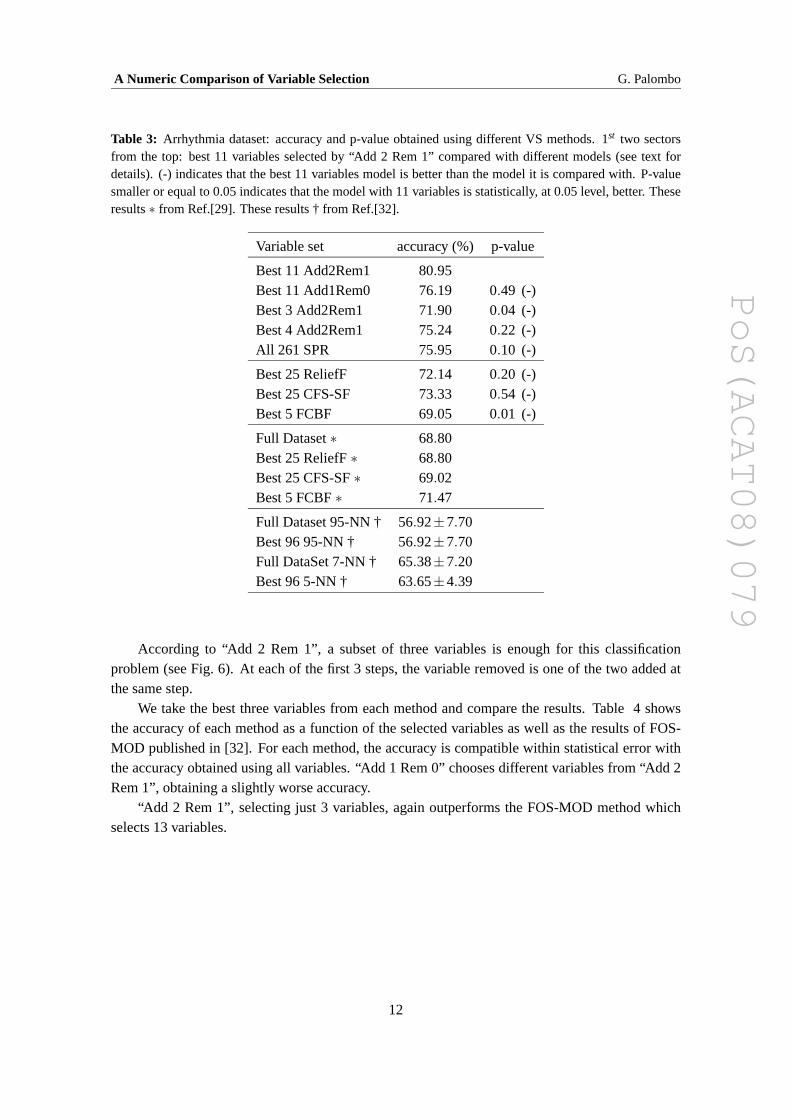
In the top sector of Table 3, the accuracy obtained by using the best 11 variables from “Add 2Rem 1” is compared with the accuracy obtained by using the best 11 variables from “Add 1 Rem 0”and the best 3 and 4 variables from “Add 2 Rem 1”; as well as with the accuracy of the full model.In the 2nd section from the top, results of the S methods implemented in Weka are compared withthe result of the 11-variable subset from “Add 2 Rem 1”. In the 3rd section from the top, we givepublished results [29] obtained with the same dataset, in a similar analysis configuration, and usingthe package Weka. Our results using ReliefF, CFS-SF and FCBF are in good agreement with thepublished results. In the bottom section of the table, we compare our results with those obtainedby the FOS-MOD method with the k-nearest-neighbor (k-NN) algorithm [32].

We use a 10-fold cross-validation paired t test [33] to compare the accuracies obtained byvarious methods. This test is widely used in machine learning applications and has the advantageof giving results independent of the specific splitting used to separate training and test sets. Toperform this test, it is necessary to know not only the average accuracyof 10-fold cross-validation,but also the accuracy of each of ten splits. Since the published results report only the averageaccuracy, we can calculate the p-values only for the results obtained by SPR and Weka.

Results of these tests are shown in table 3. “Add 2 Rem 1” and the multi-class algorithmimplemented in SPR give the best accuracy.

3.3 WDBC

Wisconsin Diagnostic Breast Cancer (WDBC) dataset has 569 events, 30 variables, and in-volves a binary classification task. The goal is to predict whether a tumor is benign or malignant.We use a random forest classifier with 50 trees, at least 2 events per leaf and 23 variables randomlychosen for each DT. The accuracy is evaluated using a 10-fold cross-validation.

VS is carried out using “Add 2 Rem 1“, “Add 1 Rem 0”, Correlations, Interactions, and FOMImportance methods implemented in SPR; as well as with the RuleFit method [34] implemented inR [9].

11

PoS(ACAT08)079


Table 3: Arrhythmia dataset: accuracy and p-value obtained using different VS methods. 1st two sectorsfrom the top: best 11 variables selected by “Add 2 Rem 1” compared with different models (see text fordetails). (-) indicates that the best 11 variables model is better than the model it is compared with. P-valuesmaller or equal to 0.05 indicates that the model with 11 variables is statistically, at 0.05 level, better. Theseresults∗ from Ref.[29]. These results † from Ref.[32].

Variable set accuracy (%) p-value

Best 11 Add2Rem1 80.95Best 11 Add1Rem0 76.19 0.49 (-)Best 3 Add2Rem1 71.90 0.04 (-)Best 4 Add2Rem1 75.24 0.22 (-)All 261 SPR 75.95 0.10 (-)

Best 25 ReliefF 72.14 0.20 (-)Best 25 CFS-SF 73.33 0.54 (-)Best 5 FCBF 69.05 0.01 (-)

Full Dataset∗ 68.80Best 25 ReliefF∗ 68.80Best 25 CFS-SF∗ 69.02Best 5 FCBF∗ 71.47

Full Dataset 95-NN † 56.92±7.70Best 96 95-NN † 56.92±7.70Full DataSet 7-NN † 65.38±7.20Best 96 5-NN † 63.65±4.39

According to “Add 2 Rem 1”, a subset of three variables is enough for this classificationproblem (see Fig. 6). At each of the first 3 steps, the variable removed isone of the two added atthe same step.

We take the best three variables from each method and compare the results.Table 4 showsthe accuracy of each method as a function of the selected variables as wellas the results of FOS-MOD published in [32]. For each method, the accuracy is compatible within statistical error withthe accuracy obtained using all variables. “Add 1 Rem 0” chooses different variables from “Add 2Rem 1”, obtaining a slightly worse accuracy.

“Add 2 Rem 1”, selecting just 3 variables, again outperforms the FOS-MODmethod whichselects 13 variables.

12

PoS(ACAT08)079


Figure 6: WDBC dataset: variation of the classification loss as a function of the best subset dimensionality.The best 3 variables selected are: WorstArea, WorstSmoothness, and WorstConcavity.

Table 4: WDBC dataset: accuracy with different variable sets. Rulefitmethod implemented in R doesn’tshow statistical errors. These results † from Ref. [32].

Variables set accuracy (%)

Full Dataset Random Forest 96.25±3.09Full Dataset RuleFit 95.78Best 3 Add2Rem1 96.07±2.77Best 3 Add1Rem0 94.89±4.29Best 3 Correlations 93.10±2.65Best 3 Permutations 96.21±2.63Best 3 Interactions 93.21±3.65Best 3 RuleFit 93.85Best 3 FOM Importance 91.25±3.20

Full Dataset† 97.94±1.67 (5-NN)13 Variables † 97.04±1.65 (7-NN)

3.4 WBC

Wisconsin Breast Cancer (WBC) dataset is similar to WDBC dataset. It has 699 events (458are benign samples and 241 are malignant) and 9 variables. We use an AdaBoost classifier withbinary splits with 100 cycles. We compare VS methods “Add 2 Rem 1”, “Add 1 Rem 0”, Corre-lations, and Interactions in SPR , RuleFit in R, and FOS-MOD [32]. As shown in Fig. 7, “Add 2Rem 1” selects three variables without loosing predictive power. At eachof the first 3 steps, “Add2 Rem 1” removes 1 of the 2 variables added at the same step. The FOS-MODmethod selects aminimum of four variables in order to not loose predictive power.

We, then, take the best three variables subset from “Add 2 Rem 1”, “Add 1 Rem 0” (same

13

PoS(ACAT08)079


Figure 7: WBC dataset: variation of classification loss as a function ofthe best subset dimensionality. Thebest 3 variables selected are: Uniformity of Cell Shape, Normal Nucleoli, and Bland Chromatin

Table 5: WBC dataset: accuracy with different variable sets. Rulefit method implemented in R does notshow statistical errors. These results † from Ref. [32].

Variables set accuracy (%)

Full Dataset Boosted Decision Split 96.24±2.59Full Dataset RuleFit 95.82Best 3 Add2Rem1 95.77±1.71Best 3 Add1Rem0 95.77±1.71Best 3 Correlations 95.28±2.54Best 3 Permutations 95.72±2.98Best 3 Interactions 94.85±3.03Best 3 RuleFit 95.61

Full Data Set † 98.16±2.03 (5-NN)4 Variables † 97.42±2.16 (15-NN)

variables as “Add 2 Rem 1”), Correlations, Interactions, and RuleFit. For each method, the resultantaccuracy is not statistically different from the one obtained using all 9 variables. In this dataset,which is particularly simple for a binary classification task, all methods give similar results, evenwhen selecting different variables, as shown in Table 5.

3.5 Colic Horse Data

Colic Horse dataset has 368 events, 22 variables and involves a binary classification task. Thetask is to predict whether the lesion is surgical. This dataset has a high number of missing valueswhich are replaced using the median value of the variable. We used a SPR tree classifier with 15as minimum number of events per leaf.

14

PoS(ACAT08)079


The output of “Add 2 Rem 1” (Fig. 8) shows that 2 variables are enoughto achieve an accuracycomparable to the one obtained with all the 22 variables. “Add 2 Rem 1”, at each of the first 2 steps,removes one of the two variables added at the same step.

Figure 8: Colic dataset: variation of classification loss as a function of the best subset dimensionality. The2 variables selected are: Surgery and Abdomal Distension.

We then evaluate the performance of VS methods implemented in SPR taking the 2 mostimportant variable from each method. In this comparison, the minimum number of events per leafof the SPR tree is taken equal to 1. In Table 6 we show the results of this study(top sectionof the table) together with published results obtained using, over the same dataset, different VSmethods and as classifiers ID3 [7] (2nd sector of the table from the top), and C4.5 [35, 36] (3rd andbottom sector of the table). In this analysis we also see a better performanceof “Add 2 Rem 1”compared to the other VS methods, since it selects fewer variables than any other published resultwhile achieving similar accuracy. The variables selected by “Correlations”give a good result too,whilst “FOM Importance” obtains the worst result among the methods implementedin SPR.

3.6 CPU Time

In Table 7 is shown the CPU time required by each method used to select the variables of thebest subset. When we run the wrapper algorithms, we use the option implemented in SPR whichallows to monitor step by step which variables are added (and also removed in case of “Add 2 Rem1”) and the corresponding classification loss at each step. That allows toselect the best subsetwithout waiting that the algorithms find the best subset for each dimensionality.This is particularlyuseful in the case of datasets with hundreds of variables, like arrhythmia dataset. “Add n Rem r”and Interactions in the magic gamma telescope analysis take longer than in any other analysis, thisis why we use a very time consuming classifier, i.e. RF with 200 cycles and 1 minimumevent perleaf, in conjunction with the largest data set (19020 events). All these experiments are conductedon a Intel Dual-Core Xeon 2.8 GHz with 1 GB RAM.

15

PoS(ACAT08)079


Table 6: Colic dataset: method, accuracy(%), and number of selectedvariables. Results on the accuracyof VS methods implemented in SPR compared with published results using different VS methods. “Add 2Rem 1” and “Add 1 Rem 0” select the same variables.

Method accuracy (%) No of sel. feat.

All 85.85±5.25Add2Rem1 85.85±5.25 2Add1Rem0 85.85±5.25 2Correlations 82.05±5.44 2Permutations 78.59±7.33 2Interactions 77.43±4.87 2FOM Importance 61.36±4.21 2

ID3 81.52±2.0 17.4ID3 HC-FSS 83.15±1.1 2.8ID3 BFS-FSS Forward 82.07±1.5 3.4ID3 BFS-FSS Backward 82.61±1.7 7.2

C4.5 GA-Wrapper 82.4 13C4.5 ReliefF-GA-Wrapper 83.8 10C4.5 ReliefF 85.3 20C4.5 All 85.3 22

C4.5-RelFss 85.9 4C4.5-RelFss’ 84.5 12

4. Summary

We have evaluated the performance of five VS methods implemented in the statistical packageStatPatternRecognition using datasets hosted at the UCI repository. We have compared their per-formance with that of other methods present in the literature. From these tests, we found that “Add2 Rem 1” has the best performance. The difference in terms of results between “Add 2 Rem 1” andthe other VS methods considered increases in significance with the complexity of the dataset. Onthe other hand, filter and embedded methods are faster. Noticeably faster ifthe dataset set is hugeand the wrapper algorithm has to interact with a time consuming classifier. In general, filter andembedded methods are often able to achieve good results; however their reliability does not seemto be guaranteed for every kind of analysis.

16

PoS(ACAT08)079


Table 7: CPU elapsed real time in minutes (m) and seconds (s) to selectthe best variables from each datasetfor all the methods used.

Dataset Events Classes Sel. variables/ Tot. variable Program Method Time

Magic 19020 2 6/10 SPR

Add 2 Rem 1 238mAdd 1 Rem 0 97m20sCorrelations 2.53sPermutations 2m58sInteractions 360m

FOM Importance 2m05s

Arrhythmia 420 1211/261 SPR

Add 2 Rem 1 44m30sAdd 1 Rem 0 19m10s

5/261Weka

FCBF 2.11s25/261 ReliefF 9.01s25/261 CFS-SF 2.65s

WDBC 569 2 3/30SPR

Add 2 Rem 1 7m52sAdd 1 Rem 0 4m29sCorrelations 0.250sPermutations 0.637sInteractions 7m20s

FOM Importance 1.02sR Rulefit 2.81s

WBC 699 2 3/9SPR

Add 2 Rem 1 12.7sAdd 1 Rem 0 4.90sCorrelations 0.078sPermutations 2.04sInteractions 23m20s

R Rulefit 2.24s

Colic 368 2 2/22 SPR

Add 2 Rem 1 2.78sAdd 1 Rem 0 1.89sCorrelations 0.142sPermutations 0.171sInteractions 30.86s

FOM Importance 0.071s

17

PoS(ACAT08)079


References

[1] K. Cranmer, Statistics for the LHC: Progress, Challenges, and Future, Proceed. of PhyStat-LHC Workshop, 47-60, Geneva, 27-29 June 2007(http://phystat-lhc.web.cern.ch/phystat-lhc/2008-001.pdf). B. P. Roe et al., Boosted DecisionTree, an Alternative to Artificial Neural Networks, Nucl. Instr. and Meth. A543, 577-584(2005).

[2] T. Hastie, R. Tibshirani and J. Friedman, The elements of Statistical Learning, Springer Seriesin Statistics, 2001; A. Webb, Statistical Pattern Recognition, John Wiley & SonsLtd, 2002.

[3] L. Breiman, J. H. Friedman, R. Olshen, and C. Stone, Classification and Regression Trees,Wadsworth and Brooks, 1984.

[4] J.R. Quinlan, Induction of decision trees, Machine Learning 1, 81-106 (1986).

[5] J. H. Friedman, Recent advances in (machine) learning, J. of Classification 23, 175-197(2006).

[6] I. Guyon et al., An introduction to variable and feature selection, J. ofMachine LearningResearch 3, 1157-1182 (2003).

[7] R. Kohavi and G. H. John, Wrappers for feature subset selection, Artificial Intelligence J.,Special Issue on Relevance 97, 273-324 (1997).

[8] https://sourceforge.net/projects/statpatrec

[9] http://www.r-project.org

[10] http://www.cs.waikato.ac.nz/ml/weka

[11] R.A. Fisher, The use of multiple measurements in taxonomic problems, Annals of Eugenics7, 179-188 (1936).

[12] J. Friedman and N. Fisher, Bump hunting in high dimensional data, Statistics and Computing9, 123-143 (1999).

[13] I. Narsky, StatPatternRecognition: A C++ Package for Statistical Analysis of High EnergyPhysics Data, axXiv:physics/0507143v1, 20 Jul 2005.

[14] S. Haykin, Neural Networks: A comprehensive Foundation, Prentice Hall, 1999.

[15] Y. Freund and R.E. Schapire, A decision theoretic generalization ofon-line learning and anapplication to boosting, Jour. of Computer and System Sciences 55, 119-139 (1997); J. Fried-man, t. Hastie and R. Tibshirani, Additive Logistic Regression: A statistical view of boosting,Annals of Statistics 28(2), 337-407 (2000).

[16] L.Breiman, Arcing Classifiers, The Annals of Statistics 26, 801-849 (1998).

18

PoS(ACAT08)079


[17] L. Breiman, Bagging Predictors, Machine Learning 26, 123-140 (1996); L. Lam and C.Y.Suen, Application of majority vote to pattern recognition: An analysis of its behaviour andperformance, IEEE Transactions on Systems, Man, and Cybernetics 27, 533-568 (1997).

[18] L. Breiman, Random Forests, Machine Learning 45, 5-32 (2001).

[19] See README in the package distribution [8].

[20] http://sf.net

[21] http://root.cern.ch

[22] R.B. Bendel and A.A. Afifi , Comparison of Stopping Rules in Forward“Stepwise” Regres-sion, J. of the American Statistical Association 72, 46-53 (1977).

[23] http://www.ics.uci.edu/~mlearn/MLRepository.htmlAsuncion, A. & Newman, D.J. (2007). UCI Machine Learning Repository, Irvine, CA: Uni-versity of California, School of Information and Computer Science.

[24] Y. Bengio, Y. Grandvalet, No unbiased estimator of the variance of k-fold cross-validation, J.of Machine Learning Research 5, 1089-1105 (2004).

[25] R. K. Bock et al., Methods for multidimensional event classification: a case study usingimages from Cherenkov gamma-ray telescope, A516, 511-528 (2004).

[26] L.Breiman, FORTRAN program Random Forests, Version 3.1, available athttp://oz.berkeley.edu/users/breiman.

[27] S.Perkins et al., Grafting: Fast, incremental feature selection by gradient descent in functionspace, J. of Machine Learning Research 3, 1333-1356 (2003).

[28] E. Allwein, R. E. Schapire and Y. Singer, Reducing Multiclass to binary: a unifying approachfor margin classifiers, J. of Machine Learning Research 1, 113-141 (2000).

[29] L. Yu and H. Liu, Efficient feature selection via analysis of relevance and redundancy, Jour.of Machime Learning Research 5, 1205-1224 (2004).

[30] M. Robnik-Sikonja and I. Kononenko, Theoretical and empirical analysis of ReliefF and RRe-liefF, Machine Learning 53, 23-69 (2003).

[31] J. R. Quinlan, C4.5:Programs for Machine Learnings, Morgan Kaufmann, 1993.

[32] H-L. Wei and S. A. Billings, Feature subset selection and ranking for data dimensionalityreduction, IEEE Trans. Pattern Analysis and Machine Intelligence 29 (1), 162-166 (2007).

[33] T. G. Dietterich, Approximate statistical tests for comparing supervisedclassification learningalgorithms, Neural Computation 10, 1895-1923 (1998).

19

PoS(ACAT08)079


[34] J. H. Friedman and B. E. Popescu,

http://www-stat.stanford.edu/~jhf/ftp/RuleFit.pdf

[35] L-X. Zhang et al., A novel hybrid feature selection algorithm: using ReliefF estimation forGA-Wrapper search, Proceed. of the Second International Conference on Machine Learningand Cybernetics, Xi’an, (2003).

[36] D. A. Bell and H. Wang, A formalism for relevance and its application infeature subsetselection, Machine Learning 41, 175-195 (2000).

20

a numeric comparison of variable selection algorithms for

Documents