This document is downloaded from DR‑NTU (https://dr.ntu.edu.sg)Nanyang Technological University, Singapore.

A novel thermal sensor concept for flow directionand flow velocity

Nguyen, Nam‑Trung

2005

Nguyen, N. T. (2005). A novel thermal sensor concept for flow direction and flow velocity.IEEE Sensors Journal, 5(6), 1224‑1234.

https://hdl.handle.net/10356/93885

https://doi.org/10.1109/JSEN.2005.858924

© 2005 IEEE. Personal use of this material is permitted. Permission from IEEE must beobtained for all other uses, in any current or future media, includingreprinting/republishing this material for advertising or promotional purposes, creating newcollective works, for resale or redistribution to servers or lists, or reuse of any copyrightedcomponent of this work in other works. The published version is available at: DOI:[http://dx.doi.org.ezlibproxy1.ntu.edu.sg/10.1109/JSEN.2005.858924].

Downloaded on 28 Feb 2022 06:10:24 SGT

1

A novel thermal sensor concept for flow directionand flow velocityNam-Trung NguyenMember, IEEE

Abstract— This paper presents an unified theory for differentmeasurement concepts of a thermal flow sensor. Based on thistheory, a new flow sensor concept is derived. The concept allowsmeasuring both direction and velocity of a fluid flow with a heaterand an array of temperature sensors. The paper first analyzesthe two-dimensional forced convection problem with a laminarflow. The two operation modes of a constant heating power andof a constant heater temperature are considered in the analyticalmodel. A novel estimation algorithm was derived for the flowdirection. Different methods for velocity measurement werepresented: hot-wire method, calorimetric method , and the novelaverage-temperature method. The only geometric parameter ofthe sensor, the dimensionless position of the sensor array, isoptimized based on the analytical results. Furthermore, the paperpresents the experimental results of the sensor prototype. Inorder to verify the analytical model, an array of temperaturesensors was used for recording the two-dimensional temperatureprofile around the heater. Temperature values are transferred toa computer by a multiplexer. A program running on a personalcomputer extracts the actual flow velocity and flow direction fromthe measured temperature data. The paper discusses differentevaluation algorithms, which can be used for this sensor. A simpleGaussian estimator was derived for the direction measurement.This estimator provides the same accuracy as the analyticalestimator. Velocity results of both calorimetric concept and thenovel average-temperature concept are also presented.

Index Terms— Thermal sensor, flow sensor, direction sensor,sensor array, heat transfer.

I. I NTRODUCTION

Commercial flow sensors for both direction and velocityare mainly based on a mechanical concept. The velocity andthe direction are measured separately. In wind measurementfor instance, both speed sensor and direction sensor are basedon the drag force. Thus, the sensor design involves movingparts, which have large sizes and require frequent maintenance.Conventional flow sensors such as Pitot probes, hot-films, andhot-wires are only capable to measure point velocity [1]. Flowdirection needs to be measured separately. Optical methodssuch as Laser Doppler Anemometry (LDA) and Particle ImageVelocimetry (PIV) need extensive measurement set-ups, whichare not suitable for rough out-door application.

The importance of thermal flow sensors for measuring thevelocity and direction of a fluid flow has been recognized inexperimental fluid mechanics and aerodynamics. The simplestconfiguration of a thermal flow sensor is an electrically heatedwire or film. This type of sensor is well established and

Manuscript received ...., 2003; revised ...., 2002.N. T. Nguyen is with School of Mechanical and Production Engineering,

Nanyang Technological University, 50 Nanyang Avenue, Singapore 639798.Email: mntnguyen@ntu.edu.sg

often referred to as hot-wire or hot-film sensor. With theemerge of micromachining technologies, micro thermal flowsensors were recently developed [2], [3], [4]. The small sizeof these sensors makes the implementation of the highly sen-sitive calorimetric concept possible [5], [6]. The calorimetricconcept uses the temperature difference between two positionsupstream and downstream of a heater for evaluating the flowvelocity. The calorimetric concept is extremely sensitive forsensors in millimeter range [7]. The major drawback of theabove thermal sensors is that they can not detect flow direction.The common practice for detecting the flow direction is the useof two one-dimensional flow sensors for measuring the twoperpendicular components of the flow velocity. The inversetangent function of the ratio between these two components isthe flow direction [4], [8], [9]. The drawback of this concept isthat the two one-dimensional flow sensors should be calibratedagainst each other, and very complex calibration proceduresare needed.

To the best knowledge of the author there were no unifiedtheory for these different measurement concepts. Furthermore,no previous work identified the direct relation between thesensor sizes and the measured velocity range.

This paper first presents an unified analytical model with alaminar flow for different thermal flow sensor concepts. Basedon this model, a new thermal flow sensor for both directionand velocity can be derived. This novel thermal flow sensorconsists of a single heater and an array of temperature sensors.Instead of measuring a single value, the sensor collects anumber of temperature values. These values are evaluatedby corresponding algorithms to extract the flow direction andvelocity.

Following the analytical model, the paper then presentsthe experimental results of a sensor prototype. The detectionof the flow direction in this concept does not need anycalibration. The measurement of the flow velocity can carriedout either with the calorimetric concept or with the novelaverage-temperature concept. The sensor presented in thispaper operates in the constant heater temperature mode.

II. T WO-DIMENSIONAL SENSOR MODEL

Figure 1 shows the model of the thermal flow sensor. Thesensor consists of a circular heater. The heater can be modelledas a linear source with a heat rate ofq′ (W/m) (Fig. 1a) or witha constant temperatureTh at the heater circumference (Fig.1b). The temperature sensing array is placed on a ring witha radiusRs. For simplification the flow direction is assumedto be θflow = 0. A rotation around z-axis in the Cartesian

2

x

y

v, To

Rh

Rs

q’q

(a)

x

y

Rh Rs

q

(b)

Th

v, To

1 2 1 2

Fig. 1. Model of the thermal flow sensor for direction and velocity:(a) constant heat rate, (b) constant heater temperature.

coordinate system or a translation of the direction angleθ inthe cylindrical coordinate system can yield the solution for theflow with a variable direction angles. The fluid flow is assumedto have a uniform velocity ofv. This model is similar to theRosenthal’s model of a moving heat source in a continuum[10]. This model was used for describing machining processessuch as welding and laser cutting [11]. However, the originalRosenthal’s model only covers a linear point source.

The inlet temperature is the reference ambient temperatureT0. The laminar flow with an uniform velocity can be assumedwith a small Reynolds-numberRe = 2Rhv/ν whereν is thekinematic viscosity of the fluid. Boundary layer effects andhydrodynamic effects behind the heater are neglected in thismodel.

Ignoring the source term for a homogenous form, the two-dimensional governing equation for the temperature field ofthe model in Fig. 1 is:

∂2T

∂x2+

∂2T

∂y2=

v

α

∂T

∂x, (1)

where α, defined by the thermal conductivityk, the heatcapacity at constant pressurecp and the densityρ:

α =k

ρcp, (2)

is the thermal diffusivity of the fluid. Equation (1) can besolved using the Rosenthal’s approach [10], where the tem-perature difference∆T is a product of a velocity-dependentpart and a symmetrical partΨ:

∆T = T − T0 = exp(vx

2α

)Ψ(x, y). (3)

Substitution of:

T = T0 + ∆T = T0 + exp( vx

2α

)Ψ(x, y) (4)

in (1) results to:

∂2Ψ∂x2

+∂2Ψ∂y2

=( v

2α

)Ψ (5)

with the boundary conditions:

∂Ψ∂x

∣∣∣x=±∞

= 0,∂Ψ∂y

∣∣∣y=±∞

= 0.

Considering the radiusr =√

x2 + y2 around the center ofthe system, the boundary condition for a linear heat source is:

∂T

∂r

∣∣∣r=Rh

= − q′

2πRhk.

In case of a constant heater temperature, the boundary condi-tion is:

T∣∣∣r=Rh

= Th.

Since the boundary conditions andΨ are symmetric withrespect tor (r ≥ Rh), equation (5) can be formulated inthe cylindrical coordinate system as:

d2Ψdr2

+1r

dΨdr

−( v

2α

)2

Ψ = 0. (6)

Equation (6) is the well know Bessel-equation [12]. Thesolution of (6) is the modified Bessel functionK0 of thesecond kind and zero order [12]:

Ψ = K0[vr/(2α)]. (7)

In the following analysis the results are non-dimentionalisedby introducing the Peclet numberPe = 2vRh/α with thediameter of the heater2Rh as the characteristic length. Theradial variable is non-dimentionalised byRh: r∗ = r/Rh.

A. Temperature field with a constant heating power

Considering the constant linear heat sourceq′ (in W/m), thesolution for the temperature difference is:

∆T (r, θ) =q′α

πkRhv−1 ×

K0[vr/(2α)]K1[vRh/(2α)]−K0[vRh/(2α)] cos θ

×exp[vr cos θ/(2α)]

exp[vRh cos θ/(2α)]. (8)

whereK1 is the Bessel function of the second kind and firstorder [12]. The asymptotic case ofv = 0 leads to the trivialcase of heat conduction, where the right side of (1) becomes0. If the dimensionless temperature difference is defined as

∆T ∗ =∆T

2q′/(πk)

The dimensionless solution of the temperature field at aconstant heating power is:

∆T ∗(r∗, θ) =K0(Per∗/4)/Pe

K1(Pe/4)−K0(Pe/4) cos θ×

{exp[Pe(r∗ − 1)/4]}cos θ. (9)

Figure 2 shows this temperature field at different Pecletnumber.

The heater temperature is a function ofθ and can beexpressed in the dimensionless form as (Fig. 3):

∆T ∗h (1, θ) =K0(Pe/4)/Pe

K1(Pe/4)−K0(Pe/4) cos θ(10)

If Pe in (10) approaches 0,T ∗h approaches the asymptoteT ∗h =1. The temperature difference∆T ∗s between the two positions

3

-10 -5 0 5 10-10

-5

0

5

10

0.1

0.1

0.1

0.1

0.2

0.2

0.2

0.2

0.3

0.30.3

0.4

0.4

0.5

0.6

-10-5

05

10

-10

0

100

0.5

1

y/Rh

DT

*

x/Rh

y/R

h

x/RhPe=1

Fig. 2. Dimensionless temperature distribution at a constant linearheat rate and Pe=1.

Pe

DT

*h

Pe

DT

*s

(a) (b)

2 4 6 8 10

0.1

0.2

0.3

0.4

0.5

0.6

0.7

0.8

0.9

1

0 2 4 6 8

0.2

0.25

0.3

0.35

0.4

0.45

R* =2s

R* =3s

R* =4s

R* =5s

R* =10s

q=0

q=p/4

q=p/2

q=3p/4

q=p

100

R* =1s

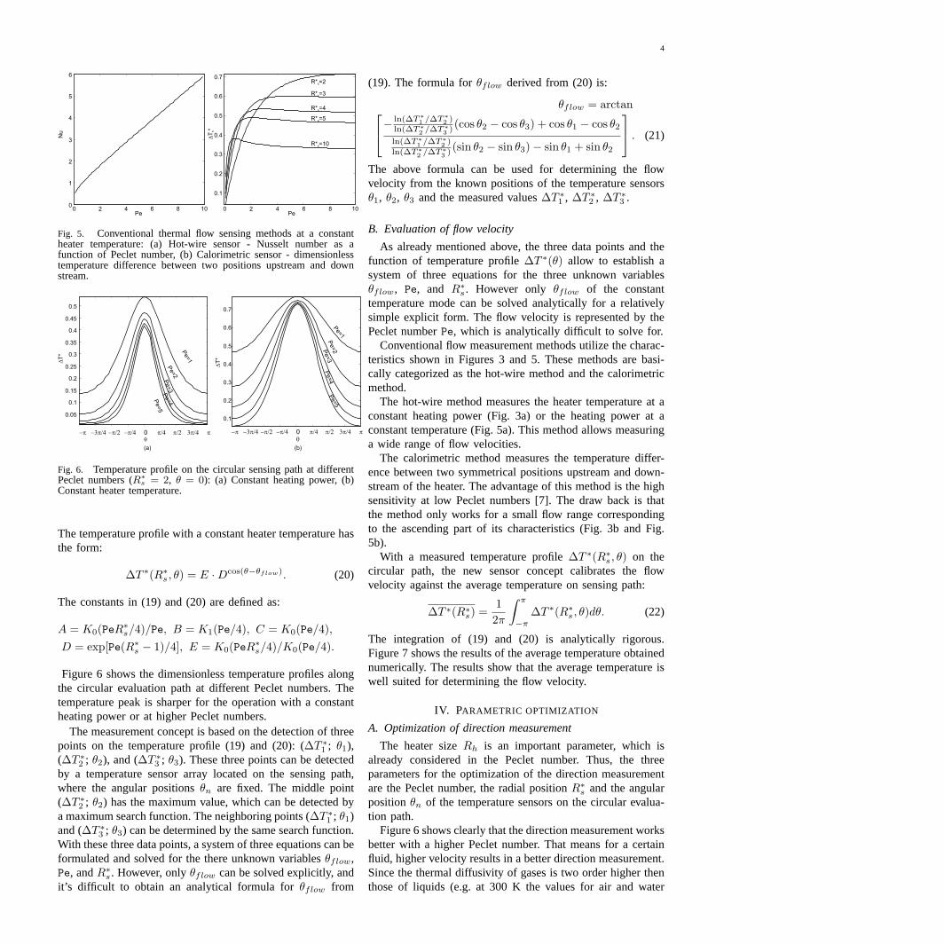
Fig. 3. Conventional thermal flow sensing methods at a constant heat-ing power: (a) Hot-wire sensor - dimensionless heater temperature atdifferent positions as a function of Peclet number, (b) Calorimetricsensor - dimensionless temperature difference between two positionsupstream and down stream.

1 and 2 on the evaluation ring (Fig. 1) across the heater inflow direction is calculated as:

∆T ∗s = ∆T ∗2 −∆T ∗1 =∆T ∗(R∗s , 0)−∆T ∗(R∗s , π) =

=K0(PeR∗s/4)

Pe{ exp[Pe(R∗s − 1)/4]K1(Pe/4)−K0(Pe/4)

− exp[−Pe(R∗s − 1)/4]K1(Pe/4) + K0(Pe/4)

} (11)

whereR∗s = Rs/Rh is the dimensionless position of the tem-perature sensors. Since∆T ∗h and∆T ∗s are functions of Pecletnumbers or the velocities of a given fluid, they can be usedfor measuring the one-dimensional flow. The correspondingmethods are called the hot-wire anemometry and calorimetricanemometry, respectively [6]. The typical characteristics of thetwo methods are shown in Fig. 3

B. Temperature field with a constant heater temperature

Considering the constant temperature boundary condition,the solution for the temperature field is:

∆T (r, θ) = ∆ThK0[vr/(2α)]

K0[vRh/(2α)]exp [vr cos θ/(2α)]

exp [vRh cos θ/(2α)](12)

By introducing the dimensionless temperature difference:

∆T ∗ = ∆T/∆Th,

x/Rh

-10 -5 0 5 10-10

-5

0

5

10

0.1

0.1

0.1

0.1

0.2

0.2

0.2

0.2

0.30.3

0.30.3

0.40.4

0.4

0.4

0.5

0.5

0.5

0.6

0.6

0.7

0.7

0.8

0.9

y/R

h

Pe=1-10

-50

510

-10

0

100

0.5

1

y/Rh

DT

*

x/Rh

Fig. 4. Dimensionless temperature distribution at a constant heatertemperature and Pe=1.

the dimensionless temperature field at a constant heater tem-perature has the form:

∆T ∗(r∗, θ) =K0(Per∗/4)K0(Pe/4)

{exp[Pe(r∗ − 1)/4]}cos θ. (13)

Figure 4 illustrates this result for different Peclet-numbers. Forthe case of the flow sensor presented in this paper, the heatrate can be represented by the dimensionless Nusselt number.Assuming a linear heat sourceq′ and a characteristic lengthof 2Rh, the Nusselt numberNu can be defined as:

Nu = q′/(πk∆Th). (14)

Using the condition at the heater circumference:

q′(θ)2πRhk

= −dT (r, θ)dr

∣∣∣r=Rh

, (15)

the heat rate at the heater circumference is:

q′(θ) =πk∆Th

2

[cos θ − K1(Pe/4)

K0(Pe/4)

](16)

From (14), the average Nusselt number of the heater is:

Nu =1

πk∆Th

12π

∫ π

−π

q′(θ)dθ =12Pe

K1(Pe/4)K0(Pe/4)

, (17)

Figure 5 shows the relation between Nusselt numbers andPeclet numbers graphically.

The temperature difference between two positions upstreamand down stream at a constant heater temperature is:

∆T ∗s =K0(PeR∗s/4)K0(Pe/4)

{exp[Pe(R∗s − 1)/4]−exp[−Pe(R∗s − 1)/4]} (18)

Both (17) and (18) are used in conventional hot-wire sensorsand calorimetric sensors to determine the flow velocity, whichis represented by the Peclet number (Fig. 5).

III. SENSING CONCEPTS AND EVALUATION ALGORITHMS

A. Evaluation of direction

The new sensing concept presented in this paper is basedon the temperature profile∆T ∗(Rs, θ) along the circular pathdefined byRs (Fig. 1). Using the dimensionless radiusR∗s =Rs/Rh of the sensing path and considering an arbitrary flowdirection θflow, the measured temperature profile along thecircular path can be derived from (9) and (13).

For a constant heating power, the temperature profile is:

∆T ∗(R∗s , θ) =A

B − C cos(θ − θflow)Dcos(θ−θflow). (19)

4

0 2 4 6 8

0.1

0.2

0.3

0.4

0.5

0.6

0.7

0 2 4 6 8 100

1

2

3

4

5

6

Pe

Nu

Pe10

R* =2s

R* =3s

R* =4s

R* =5s

R* =10s

DT

*s

Fig. 5. Conventional thermal flow sensing methods at a constantheater temperature: (a) Hot-wire sensor - Nusselt number as afunction of Peclet number, (b) Calorimetric sensor - dimensionlesstemperature difference between two positions upstream and downstream.

0.05

0.1

0.15

0.2

0.25

0.3

0.35

0.4

0.45

0.5

0 p/4 p/2 3p/4 p-p/4-p/2-3p/4-p

q

DT

*

Pe=1

Pe=2

Pe=3

Pe=4

Pe=5

(a) (b)

0.1

0.2

0.3

0.4

0.5

0.6

0.7

0 p/4 p/2 3p/4 p-p/4-p/2-3p/4-p

q

DT

*

Pe=1

Pe=2Pe=3

Pe=4

Pe=5

Fig. 6. Temperature profile on the circular sensing path at differentPeclet numbers (R∗s = 2, θ = 0): (a) Constant heating power, (b)Constant heater temperature.

The temperature profile with a constant heater temperature hasthe form:

∆T ∗(R∗s , θ) = E ·Dcos(θ−θflow). (20)

The constants in (19) and (20) are defined as:

A = K0(PeR∗s/4)/Pe, B = K1(Pe/4), C = K0(Pe/4),D = exp[Pe(R∗s − 1)/4], E = K0(PeR∗s/4)/K0(Pe/4).

Figure 6 shows the dimensionless temperature profiles alongthe circular evaluation path at different Peclet numbers. Thetemperature peak is sharper for the operation with a constantheating power or at higher Peclet numbers.

The measurement concept is based on the detection of threepoints on the temperature profile (19) and (20): (∆T ∗1 ; θ1),(∆T ∗2 ; θ2), and (∆T ∗3 ; θ3). These three points can be detectedby a temperature sensor array located on the sensing path,where the angular positionsθn are fixed. The middle point(∆T ∗2 ; θ2) has the maximum value, which can be detected bya maximum search function. The neighboring points (∆T ∗1 ; θ1)and (∆T ∗3 ; θ3) can be determined by the same search function.With these three data points, a system of three equations can beformulated and solved for the there unknown variablesθflow,Pe, andR∗s . However, onlyθflow can be solved explicitly, andit’s difficult to obtain an analytical formula forθflow from

(19). The formula forθflow derived from (20) is:

θflow = arctan−

ln(∆T∗1 /∆T∗2 )ln(∆T∗2 /∆T∗3 ) (cos θ2 − cos θ3) + cos θ1 − cos θ2

ln(∆T∗1 /∆T∗2 )

ln(∆T∗2 /∆T∗3 ) (sin θ2 − sin θ3)− sin θ1 + sin θ2

. (21)

The above formula can be used for determining the flowvelocity from the known positions of the temperature sensorsθ1, θ2, θ3 and the measured values∆T ∗1 , ∆T ∗2 , ∆T ∗3 .

B. Evaluation of flow velocity

As already mentioned above, the three data points and thefunction of temperature profile∆T ∗(θ) allow to establish asystem of three equations for the three unknown variablesθflow, Pe, and R∗s . However only θflow of the constanttemperature mode can be solved analytically for a relativelysimple explicit form. The flow velocity is represented by thePeclet numberPe, which is analytically difficult to solve for.

Conventional flow measurement methods utilize the charac-teristics shown in Figures 3 and 5. These methods are basi-cally categorized as the hot-wire method and the calorimetricmethod.

The hot-wire method measures the heater temperature at aconstant heating power (Fig. 3a) or the heating power at aconstant temperature (Fig. 5a). This method allows measuringa wide range of flow velocities.

The calorimetric method measures the temperature differ-ence between two symmetrical positions upstream and down-stream of the heater. The advantage of this method is the highsensitivity at low Peclet numbers [7]. The draw back is thatthe method only works for a small flow range correspondingto the ascending part of its characteristics (Fig. 3b and Fig.5b).

With a measured temperature profile∆T ∗(R∗s , θ) on thecircular path, the new sensor concept calibrates the flowvelocity against the average temperature on sensing path:

∆T ∗(R∗s) =12π

∫ π

−π

∆T ∗(R∗s , θ)dθ. (22)

The integration of (19) and (20) is analytically rigorous.Figure 7 shows the results of the average temperature obtainednumerically. The results show that the average temperature iswell suited for determining the flow velocity.

IV. PARAMETRIC OPTIMIZATION

A. Optimization of direction measurement

The heater sizeRh is an important parameter, which isalready considered in the Peclet number. Thus, the threeparameters for the optimization of the direction measurementare the Peclet number, the radial positionR∗s and the angularpositionθn of the temperature sensors on the circular evalua-tion path.

Figure 6 shows clearly that the direction measurement worksbetter with a higher Peclet number. That means for a certainfluid, higher velocity results in a better direction measurement.Since the thermal diffusivity of gases is two order higher thenthose of liquids (e.g. at 300 K the values for air and water

5

Pe(a)

DT

*(R

)* s

0 2 4 6 8 100

0.1

0.2

0.3

0.4

0.5

0.6

R* =1...5s

Pe(b)

2 4 6 8 10

0.2

0.4

0.6

0.8

1

R* =2s

R* =3s

R* =4s

R* =5s

R* =1s

DT

*(R

)* s

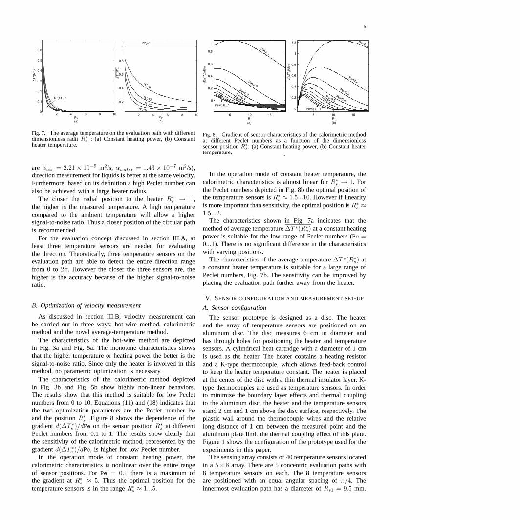
Fig. 7. The average temperature on the evaluation path with differentdimensionless radiiR∗s : (a) Constant heating power, (b) Constantheater temperature.

are αair = 2.21 × 10−5 m2/s, αwater = 1.43 × 10−7 m2/s),direction measurement for liquids is better at the same velocity.Furthermore, based on its definition a high Peclet number canalso be achieved with a large heater radius.

The closer the radial position to the heaterR∗s → 1,the higher is the measured temperature. A high temperaturecompared to the ambient temperature will allow a highersignal-to-noise ratio. Thus a closer position of the circular pathis recommended.

For the evaluation concept discussed in section III.A, atleast three temperature sensors are needed for evaluatingthe direction. Theoretically, three temperature sensors on theevaluation path are able to detect the entire direction rangefrom 0 to 2π. However the closer the three sensors are, thehigher is the accuracy because of the higher signal-to-noiseratio.

B. Optimization of velocity measurement

As discussed in section III.B, velocity measurement canbe carried out in three ways: hot-wire method, calorimetricmethod and the novel average-temperature method.

The characteristics of the hot-wire method are depictedin Fig. 3a and Fig. 5a. The monotone characteristics showsthat the higher temperature or heating power the better is thesignal-to-noise ratio. Since only the heater is involved in thismethod, no parametric optimization is necessary.

The characteristics of the calorimetric method depictedin Fig. 3b and Fig. 5b show highly non-linear behaviors.The results show that this method is suitable for low Pecletnumbers from 0 to 10. Equations (11) and (18) indicates thatthe two optimization parameters are the Peclet numberPeand the positionR∗s . Figure 8 shows the dependence of thegradientd(∆T ∗s )/dPe on the sensor positionR∗s at differentPeclet numbers from 0.1 to 1. The results show clearly thatthe sensitivity of the calorimetric method, represented by thegradientd(∆T ∗s )/dPe, is higher for low Peclet number.

In the operation mode of constant heating power, thecalorimetric characteristics is nonlinear over the entire rangeof sensor positions. ForPe = 0.1 there is a maximum ofthe gradient atR∗s ≈ 5. Thus the optimal position for thetemperature sensors is in the rangeR∗s ≈ 1...5.

5 10 15

0

0.2

0.4

0.6

0.8

5 10 15

0

0.2

0.4

0.6

0.8

1

1.2

R*s R*s

d(

T*

)/d

Ds

Pe

d(

T*

)/d

Ds

Pe

Pe=0.1

Pe=0.2

Pe=0.3Pe=0.4Pe=0.5

Pe=0.6...1

Pe=0.1

Pe=0.2

Pe=0.3Pe=0.4

Pe=0.5Pe=0.6

Pe=0.7...1

(a) (b)

Fig. 8. Gradient of sensor characteristics of the calorimetric methodat different Peclet numbers as a function of the dimensionlesssensor positionR∗s : (a) Constant heating power, (b) Constant heatertemperature. .

In the operation mode of constant heater temperature, thecalorimetric characteristics is almost linear forR∗s → 1. Forthe Peclet numbers depicted in Fig. 8b the optimal position ofthe temperature sensors isR∗s ≈ 1.5...10. However if linearityis more important than sensitivity, the optimal position isR∗s ≈1.5...2.

The characteristics shown in Fig. 7a indicates that themethod of average temperature∆T ∗(R∗s) at a constant heatingpower is suitable for the low range of Peclet numbers (Pe =0...1). There is no significant difference in the characteristicswith varying positions.

The characteristics of the average temperature∆T ∗(R∗s) ata constant heater temperature is suitable for a large range ofPeclet numbers, Fig. 7b. The sensitivity can be improved byplacing the evaluation path further away from the heater.

V. SENSOR CONFIGURATION AND MEASUREMENT SET-UP

A. Sensor configuration

The sensor prototype is designed as a disc. The heaterand the array of temperature sensors are positioned on analuminum disc. The disc measures 6 cm in diameter andhas through holes for positioning the heater and temperaturesensors. A cylindrical heat cartridge with a diameter of 1 cmis used as the heater. The heater contains a heating resistorand a K-type thermocouple, which allows feed-back controlto keep the heater temperature constant. The heater is placedat the center of the disc with a thin thermal insulator layer. K-type thermocouples are used as temperature sensors. In orderto minimize the boundary layer effects and thermal couplingto the aluminum disc, the heater and the temperature sensorsstand 2 cm and 1 cm above the disc surface, respectively. Theplastic wall around the thermocouple wires and the relativelong distance of 1 cm between the measured point and thealuminum plate limit the thermal coupling effect of this plate.Figure 1 shows the configuration of the prototype used for theexperiments in this paper.

The sensing array consists of 40 temperature sensors locatedin a 5× 8 array. There are 5 concentric evaluation paths with8 temperature sensors on each. The 8 temperature sensorsare positioned with an equal angular spacing ofπ/4. Theinnermost evaluation path has a diameter ofRs1 = 9.5 mm.

6

Heater 2R = 10mmH

Thermocouple

60 mm

5 mm

q

r

z

Fig. 9. Sensor prototype with a cylindrical heater and an array oftemperature sensors.

The other evaluation paths are placed radially 5 mm from eachother. This configuration results to five different dimensionlesssensor positionsR∗s = Rs/Rh of 1.9, 2.9, 3.9, 4.9 and 5.9. The40 thermocouples are connected to the multiplexer board of thedata acquisition unit HP 34970A, which is in turn connectedto a personal computer (PC) by the serial interface RS-232.The temperature profile above the disc is scanned and sent tothe PC where the data is processed by programs written inMATLAB.

Before further evaluation, the measured temperatures arenon-dimensionalized against the heater temperature difference∆Th = Th − T0, where Th and T0 are heater temperatureand ambient temperature respectively. The ambient tempera-ture T0 is calculated as the averaged value of all measuredtemperatures of the sensor array at non-heating condition:

T0 = 1/N

5∑

i=1

8∑

j=1

T (i, j)∣∣∣∆Th=0

, (23)

where N = 40 is the total number of temperature sensorsand T (i, j) is the temperature value of the element (i, j) inthe array. The dimensionless temperature values can then becalculated as:

∆T ∗(i, j) = [T (i, j)− T0]/[Th − T0]. (24)

Results derived from∆T ∗(i, j) are used for detecting flowvelocities and flow directions.

B. Measurement set-up

The measurement was carried out for air flow. Because ofthe relatively large size and the many wires connected to theflow sensor, the low-velocity measurement set-up described in[7] could not be used. For the calibration of the flow velocity,a mini wind tunnel was used. The test section of the windtunnel measures 10cm× 20cm. The flow velocity of the windtunnel can be varied between 5 cm/s and 40 cm/s. The flowvelocity was calibrated against a hot wire anemometer (LutronAM-4204). Because of the heater size of2Rh = 1cm, theserelatively low air flow velocities lead to a range of Pecletnumbers between 25 and 176. Thus, this experimental set-up can not characterize the ascending part of the calorimetriccharacteristics (Fig. 3b and Fig. 5b).

Temperaturecontroller

40Data

logger

HP34970AComputer

Hot-wire probe

Lutron

AM

4204

RS

232

Fan

Airflow

Thermal flow sensorLaminator

Fig. 10. Schematic concept of the measurement set-up.

-5

0

5

0

50

100

150

0

0.1

0.2

0.3

0.4

0.5

-5

0

5

0

50

100

150

0

0.1

0.2

0.3

0.4

0.5

DT

*

Pe Pex* x*

DT

*

(a) Measurement (b) Analytical model

Fig. 11. Dimensionless temperature profile across the sensor in flowdirection (experimental results versus analytical results∆T=100 K).

The flow direction was emulated by rotating the flowsensor itself. A special attachment was designed to allow apositioning accuracy of about1◦ or π/180. The measurementswere carried out in an air-conditioned ambient, where the airtemperature is kept constant at23◦C. The schematic and theactual experimental set-up are shown in Fig. 10

VI. EXPERIMENTAL RESULTS

A. Velocity measurement

Since the heater temperature is kept constant at∆Th = 100K, there are two concepts for evaluating the flow velocity:the calorimetric concept for low velocity range and the time-average concept for the high velocity range.

With a heater diameter of 1 cm, the calorimetric concept isexpected to work in the Peclet range less than 10 or for airvelocities less than 1 cm/s. Because of the limitation of theexperimental set-up, which only allows the characterization ofvelocities more then 5 cm/s, only the descending part of thesensor characteristics can be evaluated.

Figure 11 shows the temperature profile across the sensor inflow direction. Besides the slightly lower temperature as men-tioned in the previous section, the measured results agree wellwith the analytical model. Figure 12 shows the characteristicsof the calorimetric concept with five different sensor pairs.As expected, only the descending part of the characteristicscan be captured in the current experiments. The magnitude ofthe measured data is higher with a closer distance between thetemperature sensors and the heater (R∗s → 1). This observationagrees with analytical results depicted in Figures 12b and c.However, the measurement shows a stronger cooling effect.Because of the relatively low Reynolds number on the order

7

0 50 100 150 2000

0.1

0.2

0.3

0.4

0

0.2

0.4

0.6

0 50 100 150 200 0 50 100 150 2000

0.1

0.2

0.3

0.4

Pe Pe Pe

DT*s

R* =1.9s

R* =2.9s

R* =3.9s

R* =4.9sR* =5.9s

R* =1.9s

R* =2.9s

R* =3.9s

R* =4.9s

R* =5.9s

R* =1.9s

R* =2.9s

R* =3.9s

R* =4.9s

R* =5.9s

DT*s DT*s

(a)Measurement

(b)Analytical

constant heater temperature

(c)Analytical

constant heating power

0 0.1 0.2 0.3 0.4

v (m/s)

0 0.1 0.2 0.3 0.4

v (m/s)0 0.1 0.2 0.3 0.4

v (m/s)

Fig. 12. Sensor characteristics in calorimetric mode (experimentalresults versus analytical results,∆T=100 K).

(a)Measurement

(b)Analytical

constant heater temperature

0 50 100 150 2000

0.02

0.04

0.06

0.08

0.1

0

0.02

0.04

0.06

0.08

0.1

0 50 100 150 200Pe

0 0.1 0.2 0.3 0.4

v (m/s)

Pe

0 0.1 0.2 0.3 0.4

v (m/s)

DT

*(R

*)

s

DT

*(R

*)

s

R* =1.9s

R* =2.9s

R* =3.9s

R* =4.9s

R* =5.9s

R* =1.9s

R* =2.9s

R* =3.9s

R* =4.9s

R* =5.9s

Fig. 13. Sensor characteristics of the average-temperature concept(experimental results versus analytical results,∆T=100 K).

of 100, the air flow remains laminar. The discrepancy can onlyexplained with the inhomogeneous heater temperature and theboundary layer effects which are neglected in the analyticalmodel.

The average temperature on each of the five evaluation pathsis calculated as:

∆T ∗(i) =18

8∑

i=1

T ∗(i, j). (25)

The characteristics of the average-temperature concept isshown in Fig. 13. The experimental results (Fig. 13a) showthe expected characteristics of the analytical results (Fig. 13b).Evaluation paths closer to the heater yield a higher magnitude,while the sensitivity of all paths remains in almost the sameorder.

B. Direction measurement

In the direction measurement, the flow directions wereemulated by rotating the sensor relatively to the mean flowof the wind channel. The direction angleθflow was increasedfrom 0 to2π in a π/18-step. Because the innermost evaluationpath (R∗s = 1.9) always has the highest temperature, onlytheir temperature sensors are chosen in this experiment forevaluation of the flow direction.

The general evaluation algorithm starts with a search for thetemperature peak of the eight measured values of the evalu-ation path. After determining the position of the temperaturepeak (θ2,∆T ∗2 ) and its neighboring data points (θ1, ∆T ∗1 ) and(θ3,∆T ∗3 ), the flow direction is determined by the estimator

0 p/2 p 3p/2 2p 5p/2 0 p/2 p 3p/2 2p 5p/2

0

p/2

p

3p/2

2p

5p/2

0

p/2

p

3p/2

2p

5p/2

(a) (b)

qflow qflow

qestim

ate

d

qestim

ate

d

p/2-error

3p/2-error

2p-error 2p-error

Fig. 14. Characteristic of direction measurement (experimentalresults,∆T=100 K): (a) Using the analytical estimator, (b) Usingthe Gaussian estimator.

derived from the analytical model. The exact estimator (21)involves an arctan-function which may have errors atθflow =π/2 or θflow = 3π/2 because at this values the tangentfunction of direction angle approaches infinity (tan(θflow) →∞).

Because of the above mentioned problems atθflow =π/2 and θflow = 3π/2, a simpler fitting function for thetemperature peak can be used. With the direction angleθ,the fitting function∆T ∗(θ) along the circular path can bedescribed as a Gaussian distribution function:

∆T ∗(θ) = ∆T ∗max exp[− (θ − θflow)2

2σ2

], (26)

where∆T ∗max, θflow andσ are the peak value, the correspond-ing direction angle at the peak, and the variance, respectively.With the three known measured points (θ1, ∆T ∗1 ), (θ2, ∆T ∗2 )and (θ3, ∆T ∗3 ), the direction angle at the peak can be estimatedas:

θflow =(θ2

2 − θ21) ln(∆T ∗2 /∆T ∗3 )− (θ2

3 − θ22) ln(∆T ∗1 /∆T ∗2 )

2[(θ2 − θ1) ln(∆T ∗2 /∆T ∗3 )− (θ3 − θ2) ln(∆T ∗1 /∆T ∗2 )].

(27)The varianceσ and subsequently the maximum temperaturedifference∆T ∗max can be estimated as:

σ =

√(θ1 + θ2 − 2θflow)(θ2 − θ1)

2 ln(∆T ∗1 /∆T ∗2 )(28)

∆T ∗max =∆T ∗1

exp[−(θ1−θflow)2

2σ2

] . (29)

Figure 14 shows the measured direction angles with threeset of data recorded at different flow velocities (5 cm/s, 10cm/s, and 16.7 cm/s). The results show that the directionmeasurement is reproducible for different flow velocities. Asexpected the results evaluated with the analytical estimatorshow errors atθflow = π/2 and θflow = 3π/2, Fig. 14a.However, theses errors can be easily corrected by subtractingπ from the evaluated angle. Since no trigonometric function isinvolved in the Gaussian estimator, the errors atθflow = π/2andθflow = 3π/2 don’t exist, Fig. 14b. Both estimators showproblems atθflow = 0 and θflow = 2π because both anglesrepresent the same flow direction. Figure 15 compares thetwo estimators in terms of the relative errors of the directionmeasurements. The relative error (in %) is defined as:

ε = (θflow,m − θflow,a)/(π/4)× 100%, (30)

8

-100

-80

-60

-40

-20

0

20

40

60

80

100

0 p/2 p 3p/2 2p

(a)

qflow

e(%

)

-100

-80

-60

-40

-20

0

20

40

60

80

100

e(%

)

0 p/2 p 3p/2 2p

(b)

qflow

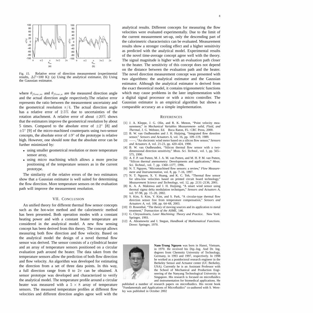
Fig. 15. Relative error of direction measurement (experimentalresults,∆T=100 K): (a) Using the analytical estimator, (b) Usingthe Gaussian estimator.

whereθflow,m and θflow,a are the measured direction angleand the actual direction angle respectively.The relative errorrepresents the ratio between the measurement uncertainty andthe geometrical resolutionπ/4. The actual direction anglehas a relative error of2.5% due to uncertainties of therotation attachment. A relative error of about±20% showsthat the estimators improve the geometrical resolution by about5 times. Compared to the absolute error of±2◦ [8] and±5◦ [9] of the micro-machined counterparts using two-sensorconcepts, the absolute error of±9◦ of the prototype is relativehigh. However, one should note that the absolute error can befurther minimized by:

• using smaller geometrical resolution or more temperaturesensor array,

• using micro machining which allows a more precisepositioning of the temperature sensors as in the currentprototype.

The similarity of the relative errors of the two estimatorsshow that a Gaussian estimator is well suited for determiningthe flow direction. More temperature sensors on the evaluationpath will improve the measurement resolution.

VII. C ONCLUSION

An unified theory for different thermal flow sensor conceptssuch as the hot-wire method and the calorimetric methodhas been presented. Both operation modes with a constantheating power and with a constant heater temperature areconsidered in the analytical model. A new flow sensingconcept has been derived from this theory. The concept allowsmeasuring both flow direction and flow velocity. Based onthe analytical model the design of a novel thermal flowsensor was derived. The sensor consists of a cylindrical heaterand an array of temperature sensors positioned on a circularevaluation path around the heater. The data taken from thetemperature sensors allow the prediction of both flow directionand flow velocity. An algorithm was developed for estimatingthe direction from a set of three data points. In this way,a full direction range from 0 to2π can be obtained. Asensor prototype was developed and characterized to verifythe analytical model. The temperature profile around a circularheater was measured with a5 × 8 array of temperaturesensors. The measured temperature profiles at different flowvelocities and different direction angles agree well with the

analytical results. Different concepts for measuring the flowvelocities were evaluated experimentally. Due to the limit ofthe current measurement set-up, only the descending part ofthe calorimetric characteristics can be evaluated. Measurementresults show a stronger cooling effect and a higher sensitivityas predicted with the analytical model. Experimental resultsof the novel time-average concept agree well with the theory.The signal magnitude is higher with an evaluation path closerto the heater. The sensitivity of this concept does not dependon the distance between the evaluation path and the heater.The novel direction measurement concept was presented withtwo algorithms: the analytical estimator and the Gaussianestimator. Although the analytical estimator is derived fromthe exact theoretical model, it contains trigonometric functionswhich may cause problems in the later implementation witha digital signal processor or with a micro controller. TheGaussian estimator is an empirical algorithm but shows acomparable accuracy an a simple implementation.

REFERENCES

[1] J. A. Kleppe, J. G. Olin, and R. K. Menon, “Point velocity mea-surement,” inMechanical Variables Measurement- solid, Fluid, andThermal, J. G. Webster, Ed. Boca Raton, FL: CRC Press, 2000.

[2] B. W. van Oudheusden and J. H. Huijsing, “Integrated flow directionsensor,”Sensors and Actuators A, vol. 16, pp. 109–119, 1989.

[3] ——, “An electronic wind meter based on a silicon flow sensor,”Sensorsand Actuators A, vol. 21-23, pp. 420–424, 1990.

[4] B. W. van Oudheusden, “Silicon thermal flow sensor with a two-dimensional direction sensitivity,”Meas. Sci. Technol., vol. 1, pp. 565–575, 1990.

[5] A. F. P. van Putten, M. J. A. M. van Putten, and M. H. P. M. van Putten,“Silicon thermal anemometry: Developments and applications,”Meas.Sci. Technol., vol. 7, pp. 1360–1377, 1996.

[6] N. T. Nguyen, “Micromachined flow sensors: a review,”Flow Measure-ment and Instrumentation, vol. 8, pp. 7–16, 1997.

[7] N. T. Nguyen, X. Y. Huang, and K. C. Toh, “Thermal flow sensorfor ultra-low velocities based on printed circuit board technology,”Measurement Science and Technology, vol. 12, pp. 2131–2136, 2001.

[8] K. A. A. Makinwa and J. H. Huijsing, “A smart wind sensor usingthermal sigma delta modulation techniques,”Sensors and Actuators A,vol. 97-98, pp. 15–20, 2002.

[9] S. Kim, S. Kim, Y. Kim, and S. Park, “A circular-type thermal flowdirection sensor free from temperature compensation,”Sensors andActuators A, vol. 108, pp. 64–68, 2003.

[10] D. Rosenthal, “The theory of moving sources and its application to metaltreatment,”Transaction of the ASME, 146.

[11] G. Chryssolouris,Laser Machining: Theory and Practice. New York:Springer, 1993.

[12] A. Abramowitz and I. Stegun,Handbook of Mathematical Functions.Dover: Springer, 1970.

Nam-Trung Nguyen was born in Hanoi, Vietnam,in 1970. He received his Dip.-Ing. And Dr. Ing.degrees from Chemnitz University of Technology,Germany, in 1993 and 1997, respectively. In 1998he worked as a postdoctoral research engineer in theBerkeley Sensor and Actuator center (UC Berkeley,USA). Currently he is an Assistant Professor withthe School of Mechanical and Production Engi-neering of the Nanyang Technological University inSingapore. His research is focused on microfluidicsand instrumentation for biomedical applications. He

published a number of research papers on microfluidics. His recent book”Fundamentals and Applications of Microfluidics” co-authored with S. Were-ley was published in October 2002