a novel multi-objective self-organizing migrating algorithm

804 P. KADLEC, Z. RAIDA, A NOVEL MULTI-OBJECTIVE SELF-ORGANIZING MIGRATING ALGORITHM

A Novel Multi-Objective Self-Organizing Migrating Algorithm

Petr KADLEC, Zbyněk RAIDA

Dept. of Radio Electronics, Brno University of Technology, Purkyňova 118, 612 00 Brno, Czech Republic

[email protected], [email protected]

Abstract. In the paper, a novel stochastic Multi-Objective Self-Organizing Migrating Algorithm (MOSOMA) is intro-duced. For the search of optima, MOSOMA employs a migration technique used in a single-objective Self Orga-nizing Migrating Algorithm (SOMA). In order to obtain a uniform distribution of Pareto optimal solutions, a novel technique considering Euclidian distances among solutions is introduced. MOSOMA performance was tested on benchmark problems and selected electromagnetic struc-tures. MOSOMA performance was compared with the per-formance of the Non-dominated Sorting Genetic Algorithm II (NSGA-II) and the Strength Pareto Evolutionary Algorithm 2 (SPEA2). MOSOMA excels in the uniform distribution of solutions and their completeness.

Keywords Multi-objective optimization, self-organizing migrating algorithm, Pareto front of optimal solutions.

1. Introduction Optimization is a mathematical process which finds

an extreme of an objective function by changing values of state variables of an optimized system. In case of an an-tenna, a main-lobe gain at a given frequency can be an objective to be maximized. Dimensions of antenna elements can play the role of state variables which are changed to maximize the gain.

In engineering, local optimization techniques are usu-ally used to improve the quality of a conventional design. Local optimization techniques can find the closest opti-mum, and therefore, the initial design has to be of a high quality. If the initial design is not in vicinity of a global optimum, local optimization methods fail.

Today’s applications require the development of unconventional solutions more and more frequently. When synthesizing an unconventional structure, basic properties of the designed structure are defined. Then, a global sto-chastic search is applied to go through the definition space of objective functions. The search is expected to reveal regions of the definition space, which obtain optima effi-ciently. For example, such orientations and lengths of seg-

ments of an antenna wire can be computed to reach a maximum gain in a given volume occupied by the an-tenna wire.

Genetic algorithms (GA) [1], particle swarm optimi-zation (PSO) [2] and self-organizing migrating algorithm (SOMA) [3, chapter 7]) belong to the most popular global stochastic optimization algorithms.

Optimization problems can comprise several con-flicting objectives with an equal importance. Then, a trade-off between objectives has to be found. For example, an antenna cannot be required for minimum dimensions and maximum gain at the same time. A solution of a multi-objective optimization leads to a set of state vectors (vectors of the dimensions of antenna elements, e. g.). Some antennas exhibit optimality from the viewpoint of gain, some are optimal from the viewpoint of dimensions.

When mapping optimal state vectors into the space of objective functions, so called Pareto front of optimal solu-tions is formed. In Fig. 1a, optimal state vectors {x1; 0} are depicted in red in the decision space. If the state vectors are mapped into the objective space (objective functions f1 and f2 are evaluated), the Pareto optimal solutions are obtained (the red curve in Fig. 1b).

No objective of the Pareto optimal solution can be improved without worsening another objective (e.g. de-creasing dimensions of the antenna decreases its gain).

Conventional methods transform a multi-objective problem into a single-objective one: partial objectives are multiplied by weighting coefficients and summed. Although this approach is simple, the setting of weights of partial objectives is problematic.

Multi-objective algorithms (MOEA) are based on the concept of the Pareto domination, which compares the mutual domination of two solutions in the objective space. The domination is defined in [4, Ch. 2, p. 28] as follows:

A solution x(1) is said to dominate another solution x(2) if both conditions 1 and 2 are true:

1. The solution x(1) is not worse than x(2) in all objec-tives.

2. The solution x(1) is strictly better than x(2) in one ob-jective at least.

RADIOENGINEERING, VOL. 20, NO. 4, DECEMBER 2011 805

0 0.5 10

0.5

1Objective space

f1 (−)

f 2 (−

)

non−optimal solutionsfeasible space bordersPareto−optimal solutions

0 0.5 1

0

0.5

1

Decision space

x1 (−)

x 2 (−

)

b)

a)

Fig. 1. Mapping from the decision space (a) into the objective

space (b) of the min-min problem.

Such a comparison can result in three cases:

1. The solution x(1) dominates the solution x(1),

2. The solution x(1) is dominated by the solution x(2),

3. The solutions x(1) and x(2) are non-dominated.

The principle of the dominance is illustrated by Fig. 2. The solution 1 dominates the solutions 2 and 3 (both the objectives f1 and f2 are smaller for the solution 1 than for the solutions 2 and 3). The solution 5 is dominated by the solution 4 (both the objectives f1 and f2 are smaller for the solution 4 than for the solution 5). Finally, the solutions 1 and 4 are members of the non-dominated set (the solution 1 excels in f1 and the solution 4 excels in f2).

The non-dominated set can be defined as follows [4, Ch. 2, p. 31]:

The non-dominated set P consists of solutions from Q, which are not dominated by any member of the set Q.

If the set Q covers the entire search space, then P be-comes the Pareto optimal set of solutions P*. Other words, P has to create the Pareto front because all other solutions from Q are dominated.

0 0.2 0.4 0.6 0.8 10

0.2

0.4

0.6

0.8

1

f1 (−)

f 2 (−

)

1

2

3

4

5

Fig. 2. The principle of the dominance.

In the open literature, the reader can find a large num-ber of multi-objective algorithms based on single-objective optimization techniques, which exploit the principle of the domination to achieve the Pareto optimal front. The non-dominated sorting genetic algorithm II (NSGA-II) [5] and the strength Pareto evolutionary algorithm (SPEA2) [6] belong to the most commonly used evolutionary algo-rithms. A comprehensive review of various multi-objective particle swarm optimizers (MOPSO) can be found in [7]. A recent multi-objective PSO-based algorithm was published in [8], which presents a comparative study of MOPSO versus NSGA-II.

In the paper, a novel multi-objective self-organizing migrating algorithm (MOSOMA) is introduced. The self-organizing migrating algorithm (SOMA) was chosen for the multi-objective implementation due to the good robust-ness and fast convergence demonstrated on many problems [3, Ch. 7, p. 189-190].

Next, a novel approach for achieving a uniform distri-bution of the resulting non-dominated set is proposed. The approach is based on the Euclidian distance between the points defining the non-dominated set.

In this paper, basic principles of multi-objective evo-lutionary algorithms (MOEA) implemented in MOSOMA are summarized. Then, section 2 reviews the single-objec-tive SOMA. The description of MOSOMA can be found in section 3. Section 4 summarizes the results obtained by MOSOMA when solving selected test problems. Section 5 proves the functionality of MOSOMA when applied on solving electromagnetic problems. Section 6 concludes the paper, highlights the advantages and disadvantages of MOSOMA and outlines the future work.

2. Single-Objective SOMA SOMA [9], [3, Ch. 7] exploits the population of indi-

viduals (agents). SOMA is based on the cooperation among


them. Although there are no new individuals created by the algorithm, SOMA can be classified as an evolutionary algorithm. The existing individuals move over an N-dimen-sional hyper-plane of the input variables according to knowledge about the researched space shared by the entire group of individuals. The algorithm can be described by the following steps:

1. Control parameters of the algorithm are defined.

2. The initial population of individuals is generated. For each individual, objective functions are evaluated.

3. According to values of the objective functions, indi-viduals are migrated. For individuals in new positions, objective functions are newly evaluated.

4. The termination condition is tested. If the termination condition is not met, the algorithm returns to step 3.

5. Solutions are assigned.

Each individual from the population of Q members is defined by the N-dimensional state vector xq. Individuals from an initial population are defined by the equation:

, min , max minq n n q n n nx x rnd x x (1)

where xq,n denotes the n-th variable of the q-th agent, ⟨xn,min; xnmax denotes the feasible interval for the n-th vari-able and rndq,n is a random number from the interval ⟨0; 1 with the uniform distribution of probability. The values of objective functions fm, where m goes from 1 to M (the number of objectives) are evaluated for each individual. These values of objective functions are shared within the population.

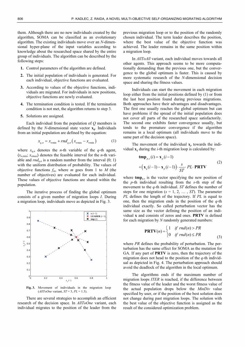
The iterative process of finding the global optimum consists of a given number of migration loops I. During a migration loop, individuals move as depicted in Fig. 3.

0 0.2 0.4 0.6 0.8 10

0.1

0.2

0.3

0.4

0.5

0.6

0.7

0.8

0.9

1

x1 (−)

x 2 (−

)

x (i−1)LEADER (i−1)tmp (i)

Fig. 3. Movement of individuals in the migration loop

(AllToOne variant, ST = 3, PL = 1.3).

There are several strategies to accomplish an efficient research of the decision space. In AllToOne variant, each individual migrates to the position of the leader from the

previous migration loop or to the position of the randomly chosen individual. The term leader describes the position, where the best value of the objective function was achieved. The leader remains in the same position within a migration loop.

In AllToAll variant, each individual moves towards all other agents. This approach seems to be more computa-tionally demanding than the previous one, but the conver-gence to the global optimum is faster. This is caused by more systematic research of the N-dimensional decision space and sharing the fitness values.

Individuals can start the movement in each migration loop either from the initial positions defined by (1) or from the last best position found during previous migrations. Both approaches have their advantages and disadvantages. The first one usually reaches the global optimum but can have problems if the spread of the initial population does not cover all parts of the researched space satisfactorily. The second one exhibits faster convergence usually, but tends to the premature convergence if the algorithm remains in a local optimum (all individuals move to the same part of the decision space).

The movement of the individual xp towards the indi-vidual xq during the i-th migration loop is calculated by:

, ( ) ( 1)

( 1) ( 1)

p s p

q p

i i

si i PL

ST

tmp x

x x PRTV (2)

where tmpp,s is the vector specifying the new position of the p-th individual resulting from the s-th step of the movement to the q-th individual. ST defines the number of steps for one migration (s = 1, 2, … , ST). The parameter PL defines the length of the trajectory. If PL is equal to one, then the migration ends in the position of the q-th individual exactly. So called perturbation vector has the same size as the vector defining the position of an indi-vidual x and consists of zeros and ones. PRTV is defined for each migration by N randomly generated numbers:

1 ( )( )

0 ( )

if rnd n PRn

if rnd n PR

PRTV (3)

where PR defines the probability of perturbation. The per-turbation has the same effect for SOMA as the mutation for GA. If any part of PRTV is zero, then the trajectory of the migration does not head to the position of the q-th individ-ual as depicted in Fig. 4. The perturbation approach should avoid the deadlock of the algorithm in the local optimum.

The algorithms ends if the maximum number of migration loops ITER is reached, if the difference between the fitness value of the leader and the worst fitness value of the actual population drops below the MinDiv value specified by user, or if the position of the best solution does not change during past migration loops. The solution with the best value of the objective function is assigned as the result of the considered optimization problem.


0 0.2 0.4 0.6 0.8 10

0.2

0.4

0.6

0.8

1

x1 (−)

x 2 (−

)

PRTV = [1,1]

PRTV = [1,0]

x (i−1)LEADER (i−1)tmp (i)

Fig. 4. Explanation of influencing migration by perturbation

(AllToOne variant, ST = 3, PL = 1.3).

Parameters controlling the run of the algorithm can be found in [3, Ch. 7, p. 173-174]. The length of the path PL should be chosen from the interval ⟨1.1; 3 . The number of steps ST during one migration loop should be from the interval ⟨3; 20 , the probability of perturbation PR should be in the interval ⟨0.1; 1.0 , the number of agents Q is ex-pected to be from the interval ⟨10; up to user , and the number of migration loops ITER is assumed to be from the interval ⟨10; up to user .

3. Description of MOSOMA MOSOMA chooses the non-dominated set of indi-

viduals from the current population in the N-dimensional decision space. The main idea of the MOSOMA is illus-trated by Fig. 7. The run of the algorithm can be described by the following steps:

1. Control parameters of the algorithm are defined.

2. The initial population of individuals is generated. For each individual, objective functions are evaluated.

3. From the current population, an external archive of non-dominated solutions is built.

4. Individuals of the current generation are migrated. Objective functions of individuals in new positions are evaluated. The external archive is updated.

5. The termination condition is tested. If the termination condition is not met, the algorithm returns to step 4.

6. The final non-dominated set of optimal solutions is chosen from the current external archive.

Since steps 1 and 2 were discussed in the previous chapter, the following subchapters will be focused on the description of steps 3 to 6. The pseudocode of the whole MOSOMA is depicted in Fig. 5.

StartBuilding initial population QEvaluation of objective functionsDetermination of external archive EXTIf |EXT| < Nex

Evaluation of crowding distanceFill in EXT with solutions from advancing fronts

EndWhile i < ITER | FFC < Nf,max | |EXT| < Nex,max

For q = 1 : |Q|q-th agent migration to all members of EXTEvaluation of objective functions

End Determination of external archive EXTIf |EXT| < Nex

Evaluation of crowding distanceFill in EXT with solutions from advancing fronts

Endi++

EndFinal non-dominated set from current EXT determination

End

Fig. 5. Pseudocode of the MOSOMA.

3.1 Choice of the Non-Dominated Set

The MOSOMA exploits an external archive [10]. The external archive EXT stores all meanwhile found members of the non-dominated set P. The searching of the non-dominated set P takes place in the objective space. The MOSOMA uses an approach introduced by Deb et al. in [4, Ch. 2, p. 36-38]. Each solution from the population of size |Q| is checked with the continuously updated P for the domination.

Comparing of all solutions to find all non-dominated solutions from Q is ineffective. Therefore, MOSOMA employs a so called continuously updated approach for the non-dominated sorting of Q defined in [4, Ch. 2, p. 36 - 38]. Each solution from Q is checked for the domination with each member of the current non-dominated set P. The working principle of this approach can be illustrated by a pseudo-code depicted in Fig. 6. Since the non-dominated set is searched in all iteration loops of MOEA, this accel-eration is important for the minimization of time devoted for the whole optimization.

Repeating the described procedure, the entire popula-tion is sorted into the fronts. Within one front, all solutions are non-dominated. Members of the first front dominate the whole rest of the solutions. Members of the second front dominate all solutions except the members of the first two fronts, etc.

The minimal size of EXT is defined by the parameter Nex. If the size of P (members of the first front) drops be-low Nex, the remaining positions are filled with members of following fronts with best values of a so called crowding distance. This metrics estimates the density of solutions


surrounding a particular solution. The crowding distance is derived from the positions of the solutions in the objective space.

StartInsert x(1) from Q to PFor i = 2 : |Q|

insert_flag = 1For j = 1 : |P|

If x(i) dominates x(j)

Remove x(i) from PEndIf x(j) dominates x(i)

insert_flag = 0Break incr. j

EndEndIf insert_flag == 1

Insert x(i) to PEnd

EndEnd

Fig. 6. The pseudo-code of the continuously updated ap-

proach for finding the non-dominated set P from set of solutions Q.

0 0.2 0.4 0.6 0.8 10

0.2

0.4

0.6

0.8

1

cuboidi−1

i

i+1

f1 (−)

f 2 (−

)

Fig. 7. Crowding distance measurement [4, Ch. 4, p. 248].

First of all, the members of one front are sorted ac-cording to all the objectives fm. The vectors of sorted indi-ces Im are found. The crowding distance c for each member of the front can be computed using the following equations [4, Ch. 4, p. 248]:

m m

1

( ) ( )M

mm

c I i c I i

(4)

where

m m

m,max ,min

( 1) ( 1)( ) m m

mm m

f I i f I ic I i

f f

(5)

where Im(i) is the i-th index from the m-th vector of indices, fm,max and fm,min are the maximal and minimal values of the m-th objective in the current front, respectively. The value

cm for these two extreme solutions is set to infinity. The crowding distance is the average side length of the cuboid defined by solutions surrounding a particular solution (see Fig. 6). The less crowded solutions (with a higher value of c) are preferred in the rest of the algorithm.

3.2 Migration of Individuals

Individuals migrate through the N-dimensional hyper-plane of input variables and try to find better solutions. MOSOMA uses the strategy called AllToMany. Each indi-vidual migrates towards all members of the external ar-chive (see Fig. 8). We assume that using equation (3) with the path length parameter PL slightly larger than one should provide new solutions, which are placed closer to the true Pareto front.

Since the size of the external archive grows with each migration loop, the time devoted for consecutive migration loops also increases. Ensuring a more accurate research of the region of current non-dominated set P is an advantage of this strategy.

0 0.2 0.4 0.6 0.8 10

0.2

0.4

0.6

0.8

1

f1 (−)

f 2 (−

)

true Pareto front

x (i−1)EXT (i−1)tmp (i)

Fig. 8. Migration of individuals to members of the external

archive in MOSOMA.

3.3 Stopping Conditions

The setting of appropriate stopping conditions is very important from the CPU time viewpoint, especially. Using the above described AllToMany strategy, the increase in the size of the external archive brings more computations of objective functions, which is usually very CPU time con-suming. In MOSOMA, the ratio of CPU-time devoted for two consecutive migration loops typically reaches high values.

Taking the previously described behavior of the algo-rithm into account, the following three stopping conditions have been formulated:

The total number of migration loops ITER is reached.

The maximal number of solutions in the external archive Nex,max (usually a multiple of the desired number of Pareto solutions Nexf) is achieved.


The maximum number of objective functions computations is performed.

Combination of these three stopping conditions should ensure that the optimization process stops in an estimable time and the sufficient number of members of the Pareto front is found.

3.4 Uniformly Spread Non-Dominated Set

Multi-objective optimizers are requested to find the non-dominated set as close to the true Pareto front as pos-sible. Moreover, optimizers are demanded to maintain the uniform spread of the non-dominated set along the true Pareto front. The difference between uniformly and non-uniformly spread non-dominated sets is shown in Fig. 9.

The crowding strategy provides the second require-ment on MOEA. In order to improve its efficiency, we propose another additional approach based on measuring Euclidian distances among the non-dominated solutions.

This strategy works with all members of the discov-ered non-dominated set P. The strategy assumes that P contains a higher number of non-dominated solutions than Nexf. First of all, the non-dominated set is sorted according to the first objective in the ascending order. Then, the length of the Pareto front e is computed by:

2

2 1

( ) ( 1)P M

m mp m

e f p f p

(6)

where fm(p) is the m-th objective function of the p-th solution, P and M denote the number of non-dominated solutions and the number of objectives, respectively.

0 0.2 0.4 0.6 0.8 10

2

4

6

8

10

f1 (−)

f 2 (−

)

true Pareto front

non−uniform setuniform set

Fig. 9. The difference between well (red) and badly (blue)

distributed non-dominated sets.

After this procedure, the ideal distance between two uniformly spread solutions eu is computed:

1u

exf

ee

N

(7)

where Nexf is the desired number of Pareto solutions. Solu-tions with minimal and maximal values of objective func-

tions are automatically assigned as the first member and the last member of the final non-dominated set Pf (considering the case with two objective functions). The j-th member of the P is that one with the minimal value dlt:

( ) ( 1) ,

2,3,..., 1

j u

exf

dlt j e j e

j N

(8)

where ej is computed using (6) while j replaces p.

This approach has to be extended for problems with more objective functions. If the Pareto front consists of more parts, all the detected discontinuous parts have to be treated separately.

4. Test Problems The proposed MOSOMA algorithm was tested on

several multi-objective test problems. Results of solving six test problems with various types of Pareto fronts are described in this chapter. Four classifiers were chosen to measure the efficiency and accuracy of the algorithm. These results are compared with results provided by commonly used multi-objective algorithms NSGA-II and SPEA2. Both the algorithms were set to provide 50 Pareto optimal solutions and to compute the objective functions 25000-times.

The total number of computation of objective func-tions FFC was the first monitored parameter (this number is not predictable when using MOSOMA). Even starting the algorithm with two identical initial populations can lead to different values of FFC due to the partially random run of the algorithm (e.g. influence of the perturbation).

As the second metric, the hit-rate HR was used [8, p. 371]:

100%

PHR

FFC (9)

where |P| is the total number of members of the non-domi-nated set, and FFC is the total number of evaluations of objective functions. Certainly, the higher values of HR indicate the better efficiency of the algorithm since only the region containing Pareto front members is researched.

The third metric, the generational distance GD was proposed by Veldhuizen in [11, Ch. 6, p. 6-15]. GD follows the line of the first demand on MOEAs, the minimal differ-ence between the members of the searched non-dominated set P and the true Pareto front P*. This metric is computed using the equation:

2

1

P

ii

d

GDP

(10)

where di is the minimal Euclidian distance in the objective space between the i-th solution from the P and any member of the true Pareto set P*:


*

2*

11

min ( ) ( )P M

i m mkm

d f i f k

(11)

where * ( )mf k is the m-th objective function value of the k-th member of P*. Usually, 500 uniformly spread members build P*. Intuitively, an algorithm with a lower value of GD is better.

The fourth metric, the spread Δ introduced by Deb in [5, p. 188] takes care of the extent of the spread among the obtained set of the non-dominated set of solutions P:

1

1 1

1

( 1)

PMem i avg

m iM

em avg

m

d d d

d P d

(12)

where di can be any distance measured between neighbor-ing solutions f(i) and f(i+1) – usually the Euclidian distance, davg denotes the mean value of these distances. Finally, e

md is the distance between the extreme solutions of P and P* corresponding to the m-th objective function. Again, an algorithm with lower value of Δ is better.

The results produced by MOSOMA and quantified by all these four metrics for six various test problems are pre-sented in the following sub-chapters. We have chosen rep-resentatives of test problems with convex, non-convex and discontinuous Pareto front. All problems minimize two objective functions only due to the simple depiction of the results. The controlling parameters for MOSOMA were set to the following values:

Size of the initial population Q = 50.

Minimal size of the external archive Nex = 20.

Size of the final non-dominated set Nexf = 50.

Maximal number of migration loops I = 10.

Maximal number of computations FFC = 25 000.

Maximal size of the external archive 5× Nexf.

Path length PL = 1.3.

The number of steps during a migration loop ST = 3.

Perturbation probability PRT = 0.1.

4.1 Simple Convex Problem

MOSOMA was tuned on a simple convex continuous test problem defined in [4, Ch. 5, p. 176] by equations:

1 1

22

1

1 2

,

1,

0.1 1, 0 5.

f x

xf

x

x x

(13)

The members of true Pareto front P* can be easily found using the equation:

*2 *

1

1.f

f (14)

Fig. 10 shows the objective space after a random run of the algorithm MOSOMA. The values of the measured metrics and their variances after 100 repetitions of the MOSOMA compared with results of NSGA-II and SPEA2 are given in Tab. 1. MOSOMA achieved better spread using less number of FFC and comparable value of GD.

0.1 0.25 0.4 0.55 0.7 0.85 1

10

20

30

40

50

60

f 1 (−)

f 2 (

−)

all researched solutionsnon−dominated setuniform non−dominated set

Fig. 10. Solutions obtained by MOSOMA in the objective

space of the simple convex problem (HR = 44.34 %, FFC = 5 981, GD = 2.79·10-5, Δ = 3.28·10-3).

Algorithm Metric HR (%) FFC (-) GD (-) Δ (-)

Average value 28.30 21317 5.32·10-3 2.08·10-2

MOSOMAVariance 151.55 8.25·108 3.15·10-6 5.74·10-2

Average value - 25000 7.20·10-3 6.53·10-1

NSGA-II Variance - - 1.10·10-5 4.30·10-3

Average value - 25000 4.50·10-3 2.77·10-1

SPEA2 Variance - - 5.90·10-7 2.01·10-4

Tab. 1. Average values of measuring metrics and their variances on simple convex problem for algorithms MOSOMA, NSGA-II and SPEA2.

4.2 Schaffer´s Test Problem

Schaffer´s test problem is probably the most studied single-variable two-objective problem. Schaffer´s test problem minimizes following objective functions:

21

22

,

( 2) ,

5 5.

f x

f x

x

(15)


The convex true Pareto optimal set can be found directly using the equation:

* * 22 1

*

( 2) ,

0 2.

f f

x

(16)

Fig. 11 shows two-dimensional objective space after a random run of the whole algorithm MOSOMA. In Tab. 2, the average values of the measured metrics and their variances after 100 repetitions for all three algorithms are given. Again, MOSOMA achieved comparable results in GD and was significantly better in Δ using less FFC in average.

0 5 10 15 20 250

15

30

45

f1 (−)

f 2 (−

)



space of Schaffer´s test problem (HR = 52.91 %, FFC = 671, GD = 1.46·10-5, Δ = 1.028·10-1).


Average value 53.46 916 7.68·10-3 5.83·10-2

MOSOMA Variance 73.39 1.16·106 2.34·10-4 3.40·10-3

Average value - 25000 3.10·10-3 5.34·10-1

NSGA-II Variance - - 1.06·10-7 1.09·10-2

Average value - 25000 3.20·10-3 1.82·10-1

SPEA2 Variance - - 5.23·10-8 4.02·10-4

Tab. 2. Average values of measuring metrics and their variances on Schaffer´s problem for algorithms MOSOMA, NSGA-II and SPEA2.

4.3 Fonseca´s Test Problem

Fonseca´s two-objective test problem is defined by:

21

1

22

1

11 exp ( ) ,

11 exp ( ) ,

4 4, 1,2,..., .

n

ii

n

ii

i

f xn

f xn

x i n

(17)

This test problem has a non-convex Pareto front given by:

2* *

2 1

*1

1 exp 2 ln(1 ) ,

0 1 exp( 4).

f f

f

(18)

We have used the simplest version with two variables only (n = 2).

0 0.2 0.4 0.6 0.8 10

0.2

0.4

0.6

0.8

1

f 1 (−)

f 2 (

−)



space of Fonseca´s test problem (HR = 11.15 %, FFC = 1961, GD = 5.31·10-6, Δ = 1.016·10-1).

The results obtained by 100 runs of MOSOMA are listed in Tab. 3. One randomly chosen Pareto front ob-tained by MOSOMA is depicted in Fig. 12. MOSOMA outperformed NSGA-II and SPEA2 in all observed metrics.


Average value 12.39 22048 1.29·10-3 9.17·10-2

MOSOMA Variance 11.56 7.89·108 1.69·10-6 6.48·10-3

Average value - 25000 2.07·10-3 5.19·10-1

NSGA-II Variance - - 2.62·10-7 1.30·10-2

Average value - 25000 1.95·10-3 1.59·10-1

SPEA2 Variance - - 1.08·10-7 3.25·10-4

Tab. 3. Average values of measuring metrics and its variances on Fonseca´s problem for algorithms MOSOMA, NSGA-II and SPEA2.

4.4 Poloni´s Test Problem

The difficulty of this problem consists in the fact, that the resulting Pareto front is convex and discontinuous. Pareto front is divided into two parts of various lengths. Unfortunately, there is no equation which could be used to define the true Pareto front. The solutions P* necessary for the computation of the metric generational distance (equa-tions (11) and (12)) were obtained thanks to a very dense sampling of regions, where the true Pareto front is located. Poloni´s test problem is defined as follows:


2 21 1 1 2 2

2 22 1 2

1

2

1 1 1 2 2

2 1 1 2 2

1 2

1 ( ) ( ) ,

( 3) ( 3) ,

0.5sin1 2cos1 sin 2 1.5cos 2,

1.5sin1 cos1 2sin 2 0.5cos 2,

0.5sin 2cos sin 1.5cos ,

1.5sin cos 2sin 0.5cos ,

, .

f A B A B

f x x

A

A

B x x x x

B x x x x

x x

(19)


Average value 23.86 16484 1.49·10-2 2.18·10-1

MOSOMA Variance 62.04 8.84·107 4.00·10-4 8.02·10-2

Average value - 25000 3.33·10-2 5.07·10-1

NSGA-II Variance - - 1.10·10-3 1.11·10-2

Average value - 25000 1.51·10-2 2.43·10-1

SPEA2 Variance - - 1.65·10-4 2.12·10-3

Tab. 4. Average values of measuring metrics and their vari-ances on Poloni´s problem for algorithms MOSOMA, NSGA-II and SPEA2.

0 10 20 30 40 50 600

10

20

30

40

50

f 1 (−)

f 2 (

−)



space of Poloni´s test problem (HR = 10.23 %, FFC = 2105, GD = 2.60·10-3, Δ = 2.30·10-1).

Fig. 13 depicts the objective space of one randomly chosen run of the MOSOMA working on Poloni´s test problem. A nice spread of solutions in both the parts of the Pareto front can be seen here. Statistic results of 100 MOSOMA runs are given in Tab. 4. MOSOMA was only slightly better in all watched metrics than SPEA2.

Solving Poloni´s test problem, an additional metric was evaluated: the number of successful identifications of a part of the Pareto front. Solving Poloni´s test problem 100 times, MOSOMA failed once only to find both parts of the Pareto front.

4.5 ZDT1 Test Problem

Zitzler et al. proposed in their paper [12] a set of six two-objective problems which can be used for the bench-mark tests and comparisons of new algorithms. The first ZDT function having 30 input variables (n = 30) is defined by:

1 1 2

2

11

, ,

9( ) 1 ,

1

( , ) 1 ,

0 1, 1, 2,..., .

N

nn

n

f x f gh

g xn

fh f g

g

x n N

x (20)

The input variables 0 ≤ x1 ≤ 1 and all other xn = 0 define the Pareto optimal region. Fig. 14 and Tab. 5 show that MOSOMA had problems with this MOOP and achieved worse results in all metrics than both algorithms used for the comparison.

0 0.2 0.4 0.6 0.8 10

2

4

6

8

10

f 1 (−)

f 2 (

−)



space of ZDT1 test problem (HR = 9.87 %, FFC = 25000, GD = 1.60·10-2, Δ = 7.27·10-1).


Average value 11.46 25000 8.52·10-2 8.12·10-1

MOSOMA Variance 15.07 - 3.79·10-3 6.37·10-3

Average value - 25000 3.35·10-2 4.72·10-1

NSGA-II Variance - - 4.75·10-3 4.26·10-2

Average value - 25000 1.43·10-2 2.08·10-1

SPEA2 Variance - - 1.48·10-6 1.22·10-3

Tab. 5. Average values of measuring metrics and their vari-ances on ZDT1 problem for algorithms MOSOMA, NSGA-II and SPEA2.


4.6 ZDT2 Test Problem

This test problem results in non-convex Pareto front. The ZDT2 has again 30 variables and its objective functions can be computed using equations:

1 1 2

2

2

11

, ,

9( ) 1 ,

1

( , ) 1 ,

0 1, 1,2,..., .

N

nn

n

f x f g h

g xn

fh f g

g

x n N

x (21)

The Pareto optimal region corresponds to 0 ≤ x1 ≤ 1 and all other xn = 0.

0 0.2 0.4 0.6 0.8 10

2

4

6

8

10

f 1 (−)

f 2 (

−)



space of ZDT2 test problem (HR = 19.23 %, FFC = 25000, GD = 4.31·10-3, Δ = 2.17·10-1).


Average value 29.08 25000 2.87·10-3 1.61·10-1

MOSOMA Variance 74.17 - 4.05·10-6 9.57·10-3

Average value - 25000 7.2410-2 4.31·10-1

NSGA-II Variance - - 3.17·10-3 4.72·10-3

Average value - 25000 1.95·10-3 2.08·10-1

SPEA2 Variance - - 1.48·10-6 1.24·10-3

Tab. 6. Average values of measuring metrics and its variances on ZDT2 problem for algorithms MOSOMA, NSGA-II and SPEA2.

MOSOMA achieved very good values of spread and generational distance in the same range as SPEA2 and better than NSGA-II as can be seen from the results presented in Fig. 15 and Tab. 6.

5. Electromagnetic Problems In this section, MOSOMA is applied to solve two

real-live problems from electromagnetics: the order reduc-

tion of Debye model for dispersive media and the multi-objective design of a waveguide partially filled with a di-electric material. Both the problems can be solved without stochastic global algorithms. The problems were selected to show the validity of a novel algorithm because the objec-tive functions can be evaluated very fast.

5.1 Debye Model Order Reduction

Dispersive materials play an important role in wide range of models. Some problems appear when time domain techniques are used. The dispersive behavior of dielectric materials can be described by the Debye model [13]. Using it, dielectric properties of the modeled material can be described by:

1 1

Nn

rn n

jj

(22)

where r is relative permittivity of the material, j is imagi-nary unit, ω is angular frequency, N is order of the Debye model, is relative permittivity for infinite frequency and n and n are the static permittivity and the relaxation time of the n-th pole respectively.

If a numerical solver considered for the analysis of the dispersive material does not allow the use of the Debye model of higher orders, the order of the model described by (22) has to be reduced. In this paper, the third order Debye model of the dispersive material Eccosorbe LS22 defined by the manufacturer is reduced to the first order model in the frequency range from 0.3 GHz up to 6.0 GHz by exploiting MOSOMA.

Input variables for the optimization are {, 1, 1}. The parameters vary in the following intervals: ∈⟨1; 15 ,1 ∈ ⟨1·10-10; 10·10-10 s and 1 ∈ ⟨1; 30 Two objective functions are defined so that the real and imaginary part of the optimized relative permittivity r,first fit the relative permittivity r,third defined by the third order model:

1 r,first r,third1

2 r,first r,third1

P

p

P

p

f real p p

f imag p p

(23)

where P is the number of frequency steps. Settings of MOSOMA remain the same as in section 4. The achieved results are again compared with commonly used algorithms NSGA-II and SPEA2. All algorithms can compute objec-tive functions at most 25000-times.

The Pareto front of the considered problem is de-picted in Fig. 16. Unfortunately, no metrics as in section 4 can be evaluated because the exact Pareto front is not known. In Fig. 16, the best results are achieved by MOSOMA because the major part of the solutions revealed by NSGA-II and SPEA2 are dominated by solutions re-vealed by MOSOMA. Also, MOSOMA covered the longest part of the Pareto front.


The relative permittivity of the first order displace-ment {3.49, 2.72·10-10, 22.74} of the Debye model chosen from the middle of the resulting Pareto front is depicted in Fig. 17. Both real and imaginary parts of the relative per-mittivity are in a very good agreement with dependencies provided by the LS22 manufacturer.

40 80 120 160 200170

200

230

260

290

320

350

f1 (−)

f 2 (−

)

SPEA2NSGA−IIMOSOMA

Fig. 16. Pareto fronts for the Debye model order reduction

problem obtained by algorithms SPEA2, NSGA-II and MOSOMA.

1 2 3 4 5 6−15

−5

5

15

25

frequency (GHz)

ε r (−

)

real 3rd Debyeimag 3rd Debyereal 1st Debyeimag 1st Debye

Fig. 17. Relative permittivity for the first order Debye model

displacement { = 3.49, 1 = 2.72·10-10, 1 = 22.74}.

5.2 Partially Filled Waveguide Design

The rectangular waveguide can be partially filled with a dielectric material (see Fig. 18) to decrease the cut-off frequency of the dominant mode [14]. Only the modes TEn,0 to z-axis can be determined:

222 2

1 1 1

222 2

2 2 2

2

2

y z

y z

nk k f

a

nk k f

a

(24)

where ky1, ky2 are wave-numbers in y-dimension for the dielectric-filled region (relative permittivity ε1 and perme-ability μ1) and air filled region, respectively. Next, f de-notes the given free-space frequency. The relation between the wave-numbers in both homogeneous parts of the wave-guide is expressed by the following equation:

1 21 1 2 2

1 2

tan tany yy y

k kk d k d

(25)

where d1 denotes the height of the dielectric material loaded into the waveguide and d2 is the height of the air-filled part. The cut-off frequency fc can be obtained from the system of equations (24) and (25), setting the propaga-tion constant kz = 0. The final equation with unknown f is transcendent and can be solved numerically using e.g. well known bisection method.

x

y

ε1, μ

1

ε2, μ

2

a

d1

d2

Fig. 18. Description of the partially filled waveguide.

Since the dielectric materials are rather expensive, we should know the price of cut-off frequency decrease when designing the partially filled waveguide. Therefore, two objective functions were formulated - f1 minimizes the cut-off frequency of the R100 waveguide (a = 22.86 mm, d1 + d2 = 10.16 mm) loaded with a dielectric material (solved from equations (24) and (25)) and f2 minimizes the cost of the dielectric material, assuming that dielectric material can be manufactured with continuous height d1 and relative permittivity 1:

1

1 12

1,max 1,max

cf f

df

d

(26)

Only two parameters are optimized: the relative per-mittivity of the dielectric material 1 ∈ ⟨1; 10 and the height of the material d1 ∈ ⟨0; 10.16 mm. Settings of all used algorithms MOSOMA, NSGA-II and SPEA2 remain the same as in the previous section. The resulting Pareto front is depicted in Fig. 19 and Pareto-optimal solutions highlighted in the decision space are depicted in Fig. 20.


Fig. 19 shows that some results found by NSGA-II are dominated by results achieved with the other algo-rithms. MOSOMA found solutions with the best spread on the Pareto front and succeeded to achieve the extreme so-lutions on the Pareto front ({f1,min; f2,max} and {f1,max; f2,min}).

2 3 4 5 6 70

0.2

0.4

0.6

0.8

1

f1 (GHz)

f 2 (−

)

SPEA2NSGA−IIMOSOMA

Fig. 19. The trade-off between cost of the dielectric material

(f2) and decrease of R100 waveguides cut-off frequency (f1).

0 2 4 6 8 100

2

4

6

8

10

d1 (mm)

ε 1 (−

)

Fig. 20. The decision space with highlighted Pareto-optimal

solutions obtained by MOSOMA.

Obviously, extreme solutions of the Pareto front cor-respond to input vectors {1 = 10; d1 = 10.16 mm} and {1 = 1; d1 = 0 mm} (R100 waveguide with no dielectric material), respectively. The centre part of the Pareto front corresponds to the input vector {1 = 2.36; d1 = 9.47 mm}.

6. Conclusions The novel MOSOMA algorithm applies the migration

strategy used in a single-objective SOMA for the scanning of the N-dimensional solution space, and the principle of dominance. MOSOMA uses an external archive to store meanwhile found non-dominated solutions, which size

changes continuously with the run of the algorithm. The non-dominated solutions are sorted using the crowding method, where less crowded solutions are preferred. A novel technique based on the comparison of Euclidian distances among the solutions constituting the non-domi-nated set is proposed to maintain the uniform spread of solutions on the Pareto front.

The change of the external archive size ensures that the regions containing the non-dominated solution are researched more precisely. Another advantage of the adap-tively changing size of the external archive can be seen in the fact that results obtained by the algorithm seem to be less sensitive on the controlling parameters (e.g. size of the initial population, minimal size of the external archive etc.). On the other hand, this behavior disallows us to know the exact number of computations of objective functions before the run of the algorithm.

MOSOMA was tested on six test problems with vari-ous types of Pareto fronts: convex (simple convex, Schaf-fer´s and ZDT1 test problems), non-convex (Fonseca´s and ZDT2 test problems) and discontinuous (Poloni´s test problem). We can state that the algorithm converges in all cases to the true Pareto front. Generally, MOSOMA achieved significantly better results of spread than SPEA2 and NSGA-II especially on test problems with lower num-ber of variables. The values of GD metric were comparable to the numbers achieved with SPEA2 and NSGA – II.

Functionality of our novel algorithm was successfully shown also on two problems from electromagnetics: Debye model order reduction and the design of the partially filled dielectric waveguide. In both cases MOSOMA achieved better or comparable results as algorithms NSGA-II and SPEA2.

In the future work, we would like to improve the efficiency of the proposed algorithm. Partially employed migration of members of the external archive to each other seems to be very promising. Also adaptive change of parameters controlling the migration of individuals (path length PL and number of steps ST) could speed up the algorithm. Identification of the optimal distribution of the initial population should also improve the efficiency of the algorithm. Thus, a sensitivity study of MOSOMA with respect to its controlling parameters should be performed.

Acknowledgements The research described in the paper has been finan-

cially supported by the Czech Science Foundation under grants no. 102/07/0688 and 102/08/H018. The research is a part of the COST action IC 0803, which is financially supported by the Czech Ministry of Education under grant OC09016. Support of the project CZ.1.07/2.3.00/20.0007 WICOMT, financed from the operational program Educa-tion for competitiveness, is gratefully acknowledged.


References [1] JOHNSON, J. M., RAHMAT-SAMII, V. Genetic algorithms in

engineering electromagnetics. IEEE Antennas and Propagation Magazine, 1997, vol.39, no.4, p.7 - 21.

[2] ROBINSON, J., RAHMAT-SAMII, Y. Particle swarm optimization in electromagnetics. IEEE Transactions on Antennas and Propagation, 2004, vol. 52, no. 2, p. 397 - 407.

[3] ONWUBOLU, G. C., BABU, B. V. New Optimization Techniques in Engineering. Berlin, Germany: Springer, 2004.

[4] DEB, K. Multi-Objective Optimization using Evolutionary Algorithms. Chichester, UK: Wiley, 2001.

[5] DEB, K., PRATAP, A., AGARWAL, S., MEYARIVAN, T. A fast and elitist multiobjective genetic algorithm: NSGA-II. IEEE Transactions on Evolutionary Computation, 2002, vol. 6, no. 2, p. 182 - 197.

[6] ZITZLER, E., LAUMANNS, M., THIELE, L. SPEA2: Improving the strength Pareto evolutionary algorithm. Technical report 103, Zürich, Switzerland: Computer Engineering and Networks Laboratory (TIK), Swiss Federal Institute of technology (ETH), 2001.

[7] REYES-SIERRA, M., COELLO COELLO, C. A. Multi-objective particle swarm optimizers: a survey of the state-of-the-art. International Journal of Computational Intelligence Research, 2006, vol. 2, no. 3, p. 287 - 308.

[8] ŠEDĚNKA, V., RAIDA, Z. Critical comparison of multi-objective optimization methods: genetic algorithms versus swarm intelligence. Radioengineering, 2010, vol. 19, no. 3, p. 369 - 377.

[9] ZELINKA, I., LAMPINEN, J. SOMA – Self organizing migrating algorithm. In Proceedings of 6th MENDEL International Conference on Soft Computing. Brno (Czech Republic), 2000, p. 76 - 83.

[10] FIELDSEND, J. E., EVERSON, R. M., SINGH, S. Using unconstrained elite archives for multiobjective optimization. IEEE Transactions on Evolutionary Computation, 2003, vol. 7, no. 3, p. 305 - 323.

[11] VELDHUIZEN, D. V. Multiobjective evolutionary algorithms: classifications, analyses and new innovations. Ph.D. Thesis, Dayton, OH, Air Force Institute of Technology. Technical report No. AFIT/DS/ENG/99-01, 1999, 270 pp.

[12] ZITZLER, E., DEB, K., THIELE, L. Comparison of multiobjec-tive evolutionary algorithms: Empirical results. Evolutionary Computation Journal, 2000, vol. 8, no. 2, p.125 - 148.

[13] MARADEI, F. A frequency-dependent WETD formulation for dispersive materials. IEEE Transactions on Magnetics, 2001, vol. 37, no. 5, p. 3303 - 3306.

[14] HARRINGTON, R. F. Time-Harmonic Electromagnetic Fields. New York, US: McGraw-Hill, 1961.

About Authors ... Petr KADLEC was born in Brno, Czech Republic on February 9, 1985. He received the B.S. and M.S. degrees in Electronics and Communications from the Brno University of Technology, Brno, Czech Republic, in 2007 and 2009, respectively. He is currently a PhD. student with the Department of Radio Electronics, Faculty of Electrical Engineering and Communication, Brno University of Technology. His current research interests include numerical methods for electro-magnetic field computations and evolutionary algorithms for the optimization of the electro-magnetic components.

Zbyněk RAIDA has graduated at the Brno University of Technology (BUT), Faculty of Electrical Engineering and Communication (FEEC). Since 1993, he has been with the Dept. of Radio Electronics FEEC BUT. In 1996 and 1997, he was with the Laboratoire de Hyperfrequences, Univer-site Catholique de Louvain, Belgium, working on varia-tional methods of numerical analysis of electromagnetic structures. Since 2006, he has been the head of the Dept. of Radio Electronics. Zbynek Raida has been working together with his students and colleagues on numerical modeling and optimization of electromagnetic structures, exploitation of artificial neural networks for solving elec-tromagnetic compatibility issues, and the design of special antennas. Zbynek Raida is a member of IEEE Microwave Theory and Techniques Society.

a novel multi-objective self-organizing migrating algorithm

Documents