a novel fluid-solid coupling framework integrating flip ...qin/research/2017-cgi-fluid-solid... ·...
TRANSCRIPT

A Novel Fluid-solid Coupling Framework Integrating FLIP andShape Matching Methods
Yang GaoState Key Laboratory of Virtual Reality Technology and
Systems, Beihang University, Beijing, China
Shuai Li∗
State Key Laboratory of Virtual Reality Technology and
Systems, Beihang University, Beijing, China
Beihang University Qingdao Research Institute, China
Hong QinDepartment of Computer Science, Stony Brook University,
New York, USA
Aimin HaoState Key Laboratory of Virtual Reality Technology and
Systems, Beihang University, Beijing, China
ABSTRACT
Physically-based fluid animation and solid deformation driven by
numerical simulation have manifested their significance for many
graphics applications during the past two decades. For example, the
fluid implicit particle (FLIP) method and shape matching technique
based on position based dynamics (PBD) have demonstrated their
unique graphics strength in fluid and solid animation, respectively.
We propose a novel integrated approach supporting the seamless
unification of FLIP and shape matching. We devise new algorithms
to tackle existing difficulties when handling new phenomena such
as high-fidelity fluid-solid interaction and solid melting. The key
innovation of this paper is a unified Lagrangian framework that
seamlessly blends FLIP and PBD based shapematching constraint to-
wards the natural yet strong coupling between fluid and deformable
solid. Within our integrated framework, it enables many compli-
cated fluid-solid phenomena with ease. We conduct various kinds
of experiments. All the results demonstrate the advantages of our
unified hybrid approach towards visual fidelity, efficiency, stability,
and versatility.
CCS CONCEPTS
•Computing methodologies →Physical simulation;
KEYWORDS
FLIP, Shape Matching, Position Based Dynamics, Solid Deformation
ACM Reference format:
Yang Gao, Shuai Li, Hong Qin, and Aimin Hao. 2017. A Novel Fluid-solid
Coupling Framework Integrating FLIP and Shape Matching Methods. In
Proceedings of CGI ’17, Yokohama, Japan, June 27-30, 2017, 6 pages.
DOI: 10.1145/3095140.3095151
∗Prof. Li is the corresponding author.
Permission to make digital or hard copies of all or part of this work for personal orclassroom use is granted without fee provided that copies are not made or distributedfor profit or commercial advantage and that copies bear this notice and the full citationon the first page. Copyrights for components of this work owned by others than ACMmust be honored. Abstracting with credit is permitted. To copy otherwise, or republish,to post on servers or to redistribute to lists, requires prior specific permission and/or afee. Request permissions from [email protected].
CGI ’17, Yokohama, Japan
© 2017 ACM. 978-1-4503-5228-4/17/06. . . $15.00DOI: 10.1145/3095140.3095151
1 INTRODUCTION
Physically-based simulations of fluids and deformable solids have
been widely studied in graphics. In particular, some applications
involve many interesting phenomena related to fluid-solid coupling
and interactions, such as solid motion and deformation, fluid cou-
pling with rigid/soft bodies, etc. However, certain difficulties still
prevail and call for novel algorithms and techniques. In this paper,
we mainly focus on the complicated dynamic interactions between
fluids and solids, offering a novel method for the complicated fluid-
solid phenomena that can not be realized by naive combination
of certain methods. We examine the fluid implicit particle (FLIP)
method, which is widely used to simulate high-quality fluid effects
because of its less numerical dissipation and better numerical sta-
bility [20]. Our improved solution is the unification of FLIP and
position-based dynamics (PBD) to streamline fluid-solid coupling
in a single framework.
The state-of-the-art methods for visually-appealing fluid anima-
tion can be roughly categorized into grid-based and particle-based
approaches. Grid-based approaches usually partition the simula-
tion domain into grid cells and calculate the physical properties at
each grid cell, such as the Lattice Boltzmann method. In contrast,
for the capture of sub-grid details, particle-based approaches are
more flexible than grid-based ones. For example, Both PBD [10]
and smoothed particle hydrodynamics (SPH) methods [14] do great
works. In recent years, FLIP becomes a very popular particle-grid
coupling method, which is good at handling incompressible fluid
with complex boundaries [5–7]. Although many great ideas have
been proposed for fluid simulation based on FLIP or FLIP-coupled
methods, FLIP based fluid-solid interactions and two-phase flu-
ids animations have not been studied as widely as SPH and PBD
methods.
In contrast, PBD methods are commonly used for solid simu-
lation with high-level stability. In this paper we will extend and
unify the incompressible FLIP method and PBD method [4, 13] to
uniformly accommodate multiple phases with ease, including de-
formation bodies, fluid-solid coupling and solid melting. Of which,
the distributions of all phases (fluids and solids) are uniformly rep-
resented by FLIP particles. The dynamics of the multi-phase system
are governed by the shape matching constraints, which serve as
constraint conditions of PBD method. Our salient contributions
can be summarized as follows:

CGI ’17, June 27-30, 2017, Yokohama, Japan Yang Gao, Shuai Li, Hong Qin, and Aimin Hao
• We propose a coupled FLIP-shape matching framework,
which enables to simultaneously simulate a much wider
range of fluid-solid phenomena.
• We propose to uniformly model the behaviors of all the
involved materials based on the same set of variables in
FLIP Navier-Stokes equations, which greatly reduce the
computation complexity.
• We propose new boundary handling method for solid and
penetration prevention measurement, which ensure the
stable and robust simulation.
2 RELATEDWORK
Since this paper mainly focuses on fluid-solid interactions, to keep
the review most relevant to our work, we briefly summarize previ-
ous works as follows.
FLIP-based fluid simulation. FLIP method is introduced to
computer graphics by Zhu et al. [20], and then it is extended to
simulate splashing water [7, 8], preserve fluid sheet [2], conduct
fluid-solid coupling [15], combine with particle methods [6], model
multi-scale droplet/spray [19], etc. For example, Ando and Selino
et al. [2, 6] respectively proposed methods to improve the particle
distribution of FLIP method. Boyd and Bridson [5] extended FLIP
method to model two-phase flows, named as MultiFLIP, which
separates velocity fields with a combined divergence formulation
to enforce overall incompressibility.
PBD based simulation. PBD is used to handle position-level
constraints based on iterative Gauss-Seidel solver [4, 12]. Many
works employ PBD for the simulation of deformable objects. For
example, Muller et al. [13] introduced a geometric constraint to
PBD for deformable object simulation, which serves as the basic
framework of our solid simulation. Bender et al. [3] proposed a
continuum-based train-energy formulation to solve the constraint
function. Tournier et al. [17] formulated a compliant constraint to
avoid instabilities due to linearization, which enables the unification
of elasticity and constraints. Meanwhile, PBD is also extended for
fluid simulation. Macklin et al. [10] proposed a set of positional
constraints to enforce constant density, and then they handled the
contact and collision of fluid-solid particles in a unified manner [11],
which is flexible enough to model various materials.
In summary, compared to the aforementioned works, we blend
FLIP and PBD based shape matching constraint towards the strong
coupling between fluid and deformable solid, using FLIP particles
for all materials instead of PBD particles. In contrast to PBD parti-
cles, FLIP particles have communication among themselves, and
the particles solely communicate via the underlying grids [7]. That
is the very reason we wish to introduce FLIP into our unified frame-
work.
3 INTEGRATED FRAMEWORK
Both FLIP and PBD methods can satisfactorily simulate a variety of
scenes, however, for some complicated phenomena such as fluid
and deformable solid interaction, they fail to provide a pleasurable
and convincing result without further improvement. The key of
our approach is a unified Lagrangian framework that blends FLIP
and PBD based shape matching constraint via natural and strong
coupling. At the numerical simulation level, we take advantages
Figure 1: Elastic bodies’ dynamics simulation based on our
method. All the particles are computed by FLIP algorithm
and the shapes are maintained by shape matching of PBD.
Shape matching constraints for
StartAdvect
particles
Mark different materialparticles
FLIP-based solver for
all particles
Deformable body (Sec 3.2)
Melting solid (Sec 4.3)
End
Enforce external forces
Boundary modification& Penetration
Prevention (Sec 4.1&4.2)
Updateparticles
Figure 2: Thepipeline of our integrated framework. Theblue
squares represent the normal FLIP algorithms, and the gray
ones represent our improvements being coupled in FLIP
framework.
of MultiFLIP and shape matching. The dynamics of particles are
solved by MultiFLIP solver, and the deformation of solid is handled
by shape matching constraint. Our hybrid framework consists of
three main components: (1) the uniform solution of all particles in
a FLIP framework; (2) the coupling of FLIP simulation and shape
matching constraint; (3) the correction of particles to ensure the
accuracy and stability of FLIP solver. And the pipeline of our inte-
grated framework is shown in Fig. 2, which illustrates it can support
seamless unification of FLIP and shape matching.
3.1 The Unified Algorithm
Take fluid-solid interaction for example, Algorithm 1 shows the
main process within a time interval Δt . The texts marked in blue
highlight our method’s contributions, which improve the standard
MultiFLIP simulation for hybrid fluid-solid simulation. During
initialization, we mark different materials with different flags (e.g.,
Fsolid ,Ff luid ). FLIP solver provides two positions (x0p and xp) for
each solid particle, which can respectively be used as the original
and predicted position for shape matching constraint. So we can
apply the shape matching constraint to solid particles directly to
simulate solid bodies movements (Fig 1).

A Novel Fluid-solid Coupling Framework Integrating FLIP and Shape Matching Methods CGI ’17, June 27-30, 2017, Yokohama, Japan
Algorithm 1 Implementation of our integrated framework for
fluid-solid simulation.
1: Advect velocities of particles
2: Enforce external forces (gravity)
3: Verify fluid and solid particle flags by Fsolid ,Ff luid4: Map all particles to grid u0g ← u0p, x
0g ← x0p
5: Compute level set Φ and velocity on grid ug6: Project up ← ug, xp ← x0g + ugΔt7: if particle ∈ Fsolid then
8: Project shape matching constraint
9: Compute target position g
10: Update x∗p+=α(g − xp
)11: Update u∗p ← (up, (x
∗p − x0p)/Δt)
12: else Continue
13: Correct boundary conditions
14: Perform mechanism of penetration prevention
15: Update the velocities and positions of all particles
16: Update particles’ flags
3.2 Integrated Formulations
When getting the particle velocity of solid, we compute a predicted
position for this particle via
xp = x0p + upΔt , (1)
and x0p is the initial position, and uд is the projected velocity from
FLIP solver.
The target position is computed via
g = Csm (xp , x0p ) × (x0p − x0cm ) + xcm , (2)
with predicted mass center x0cm , and Csm (xp , x0p ) is the shape
matching constraint related to the initial and predicted positions.
Thus, new particle position is computed as:
x∗p = x∗p + α(g − xp ). (3)
The computations in line 10 and line 11 of Algorithm 1 are the same
as the traditional PBD method, wherein x∗p will be updated toward
the final position of each particle. And we update the new velocity
u∗p by a combination of FLIP-velocity up and displacement-velocity:
u∗p =
(up +
(x∗p − x0p
))/Δt)
2. (4)
With the hybrid framework, we can simulate fluid interactions
with various materials ranging from stiff solids to viscoplastic bod-
ies. However, since the new values are directly computed based on
a PBD constraint, which involves no restrictions related to bound-
aries and FLIP fluid, the fluid particles may penetrate into solid, or
the solid particles may move out of the defined boundary. Thus,
boundary conditions need be added to solid and fluid particles
to guarantee the stability, and the penetration prevention mea-
surement should be introduced to guarantee physical reality and
accuracy.
To track the sharp interface between different materials, we
respectively use two sets of independent matching-cube algorithms
to capture the fluid and solid (or some other materials’) surfaces.
And we use the boundary particles of the solid to sample the surface
(a) (b)
Virtual boundary
Boundary
Figure 3: Illustration of solid boundary conditions. When
a solid particle penetrates into the virtual boundary (dotted
line), we give it an inverse velocity depending on the posi-
tion P and the position of virtual boundary grid P0.
of objects [1], which allows handling different shapes, such as lower-
dimensional rigid bodies. The flag of each particle indicates which
system it belongs to, ensuring the accurate demarcation of different
materials.
4 BOUNDARY HANDLING ANDIMPLEMENTATION DETAILS
With our hybrid framework, we can simulate fluid flows and im-
itate a solid simulator with shape matching constraint. However,
since the naive coupling will suffer from serious numerical and
stability problems [9], we will introduce our novel measurements
into the hybrid framework to realize accurate simulations and rich
applications.
4.1 Boundary Handling for Solid
In our hybrid solver, fluid grid interacting with boundary grid will
rebound in an inverse direction. But for solid, since a set of particles
are clustered together, if we take the same boundary conditions
as fluid, local movements of the particles on boundary grids will
lead to unrealistic global deformation, and affect the simulation
stability. Thus, we define a new boundary condition for solid. For a
set of solid particles, we allow transitory penetration into a virtual
boundary grid to keep the global shape unchanged. The virtual
boundary grid is defined as:{Pmin = Xmin + λh,
Pmax = Xmax − λh.(5)
Here Xmax is the maximum position of the boundary grid, and
Xmin is the minimum position of the boundary grid, Pmin and
Pmax are the virtual boundary locations, and h is the grid size of
FLIP. λ ∈ [0, 1] controls the shrinkage degree of virtual boundary.
When λ = 0, the virtual boundary is equal to real boundary. In
most of our experiments, we set λ = 0.3, which can effectively
avoid penetrating into the real boundary and can handle the solid
interactions well.
As shown in Fig. 3(a), P is the position of solid particle that
penetrates into virtual boundary, and P0 is the position of the
virtual boundary grid. When solid particle moves across the virtual
boundary, we compute its inverse velocity (shown in Figure 3(b))

CGI ’17, June 27-30, 2017, Yokohama, Japan Yang Gao, Shuai Li, Hong Qin, and Aimin Hao
cn cn
relv relv
nrelv
trelv
ipip
Solid cvpv
(a) (b)
Figure 4: Penetration prevention for particles. vnrel
, vtr el
are
the relative velocities along the normal and tangential direc-
tions.
by
u′
=
{u∗ + γ (P0 − P) × N , P < Pmin
u∗ − γ (P − P0) × N , P > Pmin. (6)
Here γ is a bounce parameter that can be taken as the boundary
elasticity, and N is the total number of solid particles. Because solid
particles’ number relates to the mass of the solid body, the more
particles a solid body has the larger inertia it carries.
4.2 Penetration Prevention Measurement
When simulating fluid-solid interactionswith particle-basedmethod,
an indispensable work is to prevent fluid particle from penetrat-
ing into solid particles. Inspired by the position correction idea
used for smooth interface [5], we develop an additional algorithm
to prevent particle penetration. First, after updating the particles’
positions and velocities, we detect collision between solids and
fluid particles. For each fluid particle Pi , we search solid particles
that collide with Pi , and determine the collision positions. Second,
we compute the relative velocity between the fluid and the solid
particle by vr el = vp − vc , as shown in Fig. 4(a). When the relative
velocity points into the solid, i.e., vr el · nc is negative, penetration
occurs. To prevent it we impose a fluid-solid boundary condition
on the velocity of fluid particle vp as:
vnewp = vp − vnrel= vp − (vr el · nc )nc , (7)
where the relative velocity along the normal direction vnrel
is sub-
tracted to make the particle’s velocity equals to the solid’s velocity
in the normal direction.
In fact, the above velocity correction on fluid particle is equiva-
lent to enforcing an impulse on the particle. To conservemomentum
during the collision handling, we compute the collision force and
impose this force on the solid via
f =mp (vr el · nc )nc
Δt. (8)
4.3 Melting Simulation
Each particle is attached by a material flag in order to identify which
material it belongs to, and and the phase change process will be
in charge of the flag updating, which also serves as the criterion
that guides us to design the dynamic algorithm accordingly. So for
Figure 5: Illustration of heat transfer among solids and liq-
uids. The particles are colored according to temperatures
(blue means low and red means high).
Table 1: Performance of experiments.
Scenes Total Grid size Avg. time Rendering time
particles /Timestep(ms) /Frame(s)
Fig. 1 390k 643 79.33 12.95
Fig. 6 80k (fluid) 643 82.06 9.75
Fig. 7 680k 1282 × 64 138.68 17.67
Fig. 8 60k (fluid) 643 71.32 7.37
each particle, we update its temperature in each time step, and then
determine whether its phase needs to be changed or not.
To simulate melting, we initiate all the particles with a tempera-
ture attribute, the temperature update only depends upon the heat
transfer. In each time step, temperature is mapped from particles
to each grid cell with a weighting function:
Tn+1 −Tn
Δt= b(∂2Tn+1
∂x2+∂2Tn+1
∂y2+∂2Tn+1
∂z2), (9)
where Tn is the given temperature field obtained in the last time
step, Tn+1 is the current one we need to update, and b is the
corresponding thermal diffusivity parameter. After updating the
temperature on grid Tn+1д , we map the temperature changes of
the grid to particles, and then update the particle temperature by
Tn+1p = Tnp +ΔTp . When the temperature of a solid particle reaches
to melting point, convert it to a fluid particle and alter it with the
fluid’s attributes, then release it from being confined as solid. Thus,
this particle will become a free fluid particle, while the other solid
particles still hold the integrity of solid constraints. Fig. 5 shows
the heat transfer process.
5 EXPERIMENTS AND EVALUATIONS
We implement our method on a PC with an NVIDIA Geforce GTX
1080 GPU, Intel Core I7 CPU using c++ and CUDA. And we demon-
strate the capabilities of our hybrid framework via several simula-
tion scenarios. Table 1 documents the performance of our exper-
iments, indicating the high efficiency of our CUDA-based imple-
mentation.
5.1 CUDA-based Numerical Computation
We implement the entire modeling framework based on CUDA for
efficiency. For each particle, we invoke a CUDA thread to calculate
which grid cell it belongs to, and then use a CUDA thread for
each grid cell to interpolate its velocity from particles. Table 2
A Novel Fluid-solid Coupling Framework Integrating FLIP and Shape Matching Methods CGI ’17, June 27-30, 2017, Yokohama, Japan
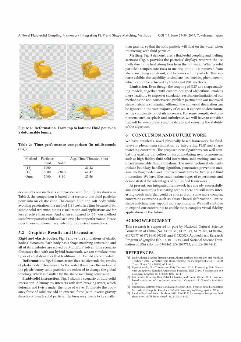
Figure 6: Deformation. From top to bottom: Fluid pours on
a deformable bunny.
Table 2: Time performance comparison (in milliseconds
(ms)).
Method Particles Avg. Time/Timestep (ms)
Fluid Solid
[18] 5000 - 21.32
[16] 5000 23095 62.47
Ours 5000 8199 25.56
documents our method’s comparison with [16, 18]. As shown in
Table 2, the comparison is based on a scenario that fluid particles
pour into an elastic cone. To couple fluid and soft body while
avoiding penetration, the method [18] costs less time because of its
simple solid structure, but its visualization and applications are far
less effective than ours. And when compared to [16], our method
uses fewer particles while still achieving better performance. Please
refer to our supplementary video for more vivid animations.
5.2 Graphics Results and Discussion
Rigid and elastic bodies. Fig. 1 shows the simulations of elastic
bodies’ dynamics. Each body has a shape matching constraint, and
all of its attributes are solved by MultiFLIP solver. This scenario
illustrates that, with our hybrid framework, we can simulate most
types of solid dynamics that traditional PBD could accommodate.
Deformation. Fig. 6 demonstrates the realistic rendering results
of plastic body deformation. As the water flows over the surface of
the plastic bunny, solid particles are enforced to change the global
topology, which is handled by the shape matching constraint.
Fluid-solid interaction. Fig. 7 shows a scenario of fluid-solid
interaction. A bunny toy interacts with dam-breaking water, which
deforms and twists under the force of wave. To imitate the buoy-
ancy force of solid, we add an external force (with inverse gravity
direction) to each solid particle. The buoyancy needs to be smaller
than gravity, so that the solid particle will float on the water when
interacting with fluid particles.
Melting. Fig. 8 demonstrates a fluid-solid coupling and melting
scenario (Fig. 5 provides the particles’ display), wherein the ice
melts due to the heat absorption from the hot water. When a solid
particle’s temperature rises to melting point, it is removed from
shape matching constraint, and becomes a fluid particle. This sce-
nario exhibits the capability to simulate local melting phenomenon,
which cannot be achieved by traditional PBD methods.
Limitation. Even though the coupling of FLIP and shape match-
ing models, together with custom-designed algorithms, enables
more flexibility to empower simulation results, one limitation of our
method is the non-conservation problem pertinent to our improved
shape matching constraint. Although the numerical dissipation can
be ignored in the vast majority of cases, it expects to deteriorate
as the complexity of details increases. For some complicated phe-
nomena such as splash and turbulence, we will have to consider
tradeoff between preserving the details and ensuring the stability
of the algorithm.
6 CONCLUSION AND FUTUREWORK
We have detailed a novel physically-based framework for fluid-
relevant phenomena simulation by integrating FLIP and shape
matching constraint. The proposed new algorithms can well com-
bat the existing difficulties in accommodating new phenomena,
such as high-fidelity fluid-solid interaction, solid melting, and two-
phase immiscible fluid animation. The novel technical elements
include boundary handling algorithm, penetration prevention mea-
sure, melting model, and improved constraints for two-phase fluid
interaction. We have illustrated various types of experiments and
demonstrated the advantages of our unified framework.
At present, our integrated framework has already successfully
simulated numerous fascinating scenes, there are still many inter-
esting constraints that could be chosen from, some more complex
constraint extensions such as cluster-based deformation, lattice
shape matching may support more applications. We shall continue
to expand our constraints to enable more complex visual-fidelity
applications in the future.
ACKNOWLEDGMENT
This research is supported in part by National Natural Science
Foundation of China (No. 61190120, 61190124, 61190125, 61300067,
61672077, 6167214, 61602341 and 61532002), Applied Basic Research
Program of Qingdao (No. 16-10-1-3-xx) and National Science Foun-
dation of USA (No. IIS-0949467, IIS-1047715, and IIS-1049448).
REFERENCES[1] Nadir Akinci, Markus Ihmsen, Gizem Akinci, Barbara Solenthaler, and Matthias
Teschner. 2012. Versatile rigid-fluid coupling for incompressible SPH. ACMTrans. Graph. 31, 4 (2012), 62:1–62:8.
[2] Ryoichi Ando, Nils Thurey, and Reiji Tsuruno. 2012. Preserving Fluid Sheetswith Adaptively Sampled Anisotropic Particles. IEEE Trans. Visualization andComputer Graphics 18, 8 (2012), 1202–1214.
[3] Jan Bender, Koschier Dan, Patrick Charrier, and Daniel Weber. 2014. Position-based simulation of continuous materials. Computers & Graphics 44 (2014),1–10.
[4] Jan Bender, Matthias Muller, and Miles Macklin. 2015. Position-Based SimulationMethods in Computer Graphics. Tutorial Proceedings of Eurographics (2015).
[5] Landon Boyd and Robert Bridson. 2012. MultiFLIP for energetic two-phase fluidsimulation. ACM Trans. Graph. 31, 2 (2012), 1–12.

CGI ’17, June 27-30, 2017, Yokohama, Japan Yang Gao, Shuai Li, Hong Qin, and Aimin Hao
Figure 7: Fluid-solid interaction. From top to bottom: Fluid interacts with a deformable bunny.
Figure 8: Melting simulation. Fluid pours on a meltable
bowl, and the bowl continuously melts.
[6] Jens Cornelis, Markus Ihmsen, Andreas Peer, and Matthias Teschner. 2014. IISPH-FLIP for incompressible fluids. Computer Graphics Forum 33, 2 (2014), 255–262.
[7] Florian Ferstl, Ryoichi Ando, ChrisWojtan, RdigerWestermann, andNilsThuerey.2016. Narrow Band FLIP for Liquid Simulations. International Journal forNumerical Methods in Fluids 35, 2 (2016), 225–232.
[8] Dan Gerszewski and Adam W. Bargteil. 2013. Physics-based Animation ofLarge-scale Splashing Liquids. ACM Trans. Graph. 32, 6 (2013), 1–6.
[9] Markus Huber, Bernhard Eberhardt, and Daniel Weiskopf. 2015. BoundaryHandling at Cloth-Fluid Contact. Computer Graphics Forum 34, 1 (2015), 14–25.
[10] Miles Macklin and Matthias Muller. 2013. Position Based Fluids. ACM Trans.Graph. 32, 4 (2013), 1–12.
[11] Miles Macklin, Matthias Muller, and Nuttapong Chentanez. 2016. XPBD: Position-Based Simulation of Compliant Constrained Dynamics. Motion in Games (2016),491–54.
[12] Matthias Muller, Bruno Heidelberger, Marcus Hennix, and John Ratcliff. 2007. Po-sition based dynamics. Journal of Visual Communication & Image Representation18, 2 (2007), 109–118.
[13] Matthias Muller, Bruno Heidelberger, Matthias Teschner, and Markus Gross.2005. Meshless deformations based on shape matching. ACM Trans. Graph. 24, 3(2005), 471–478.
[14] Andreas Peer and Matthias Teschner. 2016. Prescribed Velocity Gradients forHighly Viscous SPH Fluids with Vorticity Diffusion. IEEE Trans. Visualizationand Computer Graphics PP, 99 (2016), 1–1.
[15] A Selino and MD Jones. 2013. Large and small eddies matter: Animating trees inwind using coarse fluid simulation and synthetic turbulence. Computer GraphicsForum 32, 1 (2013), 75–84.
[16] X. Shao, Z. Zhou, N. MagnenatfiQuThalmann, and W. Wu. 2015. Stable and FastFluid-Solid Coupling for Incompressible SPH. Computer Graphics Forum 34, 1(2015), 191–204.
[17] Maxime Tournier, Matthieu Nesme, and Benjamin Gilles. 2015. Stable constraineddynamics. ACM Trans. Graph. 34, 4 (2015), 1–10.
[18] Lipeng Yang, Shuai Li, Aimin Hao, and Hong Qin. 2012. Realtime Two-WayCoupling of Meshless Fluids and Nonlinear FEM. Computer Graphics Forum 31,7 (2012), 2037–2046.
[19] Lipeng Yang, Shuai Li, Aimin Hao, and Hong Qin. 2014. Hybrid Particle-gridModeling for Multi-scale Droplet/Spray Simulation. Computer Graphics Forum33, 7 (2014), 199–208.
[20] Yongning Zhu and Robert Bridson. 2005. Animating sand as a fluid. ACM Trans.Graph. 24, 3 (2005), 965–972.