Pattern Recognition Letters 41 (2014) 23–33

Contents lists available at ScienceDirect

Pattern Recognition Letters

journal homepage: www.elsevier .com/locate /patrec

A novel associative model for time series data mining q

0167-8655/$ - see front matter � 2013 Elsevier B.V. All rights reserved.http://dx.doi.org/10.1016/j.patrec.2013.11.008

q This paper has been recommended for acceptance by Jesús Ariel CarrascoOchoa.⇑ Corresponding author. Tel.: +52 (55) 57296000x52535.

E-mail addresses: ilopezy@ipn.mx (I. López-Yáñez), sher@imp.mx(L. Sheremetov), cyanez@cic.ipn.mx (C. Yáñez-Márquez).

URL: http://www.alfabeta.org.mx (C. Yáñez-Márquez).

Itzamá López-Yáñez b,⇑, Leonid Sheremetov a, Cornelio Yáñez-Márquez c

a Mexican Petroleum Institute (IMP), Av. Eje Central Lázaro Cárdenas Norte 152, Mexico City, Mexicob Instituto Politécnico Nacional, Centro de Innovación y Desarrollo Tecnológico en Cómputo (CIDETEC – IPN), Av. Instituto Politécnico Nacional 2580, Mexico City, Mexicoc Instituto Politécnico Nacional, Centro de Investigación en Computación (CIC – IPN), Av. Juan de Dios Bátiz s/n Edificio CIC, Mexico City, Mexico

a r t i c l e i n f o a b s t r a c t

Article history:Available online 23 November 2013

Keywords:Time series data miningSupervised classificationAssociative modelsMackey–Glass benchmarkCATS benchmarkOil production time series

The paper describes a novel associative model for time series data mining. The model is based on theGamma classifier, which is inspired on the Alpha–Beta associative memories, which are both supervisedpattern recognition models. The objective is to mine known patterns in the time series in order to forecastunknown values, with the distinctive characteristic that said unknown values may be towards the futureor the past of known samples. The proposed model performance is tested both on time series forecastingbenchmarks and a data set of oil monthly production. Some features of interest in the experimental datasets are spikes, abrupt changes and frequent discontinuities, which considerably decrease the precision oftraditional forecasting methods. As experimental results show, this classifier-based predictor exhibitscompetitive performance. The advantages and limitations of the model, as well as lines of improvement,are discussed.

� 2013 Elsevier B.V. All rights reserved.

1. Introduction

Time series (TS) analysis has become a relevant tool for under-standing the behavior of different processes, both naturally ocur-ring and human caused (Pollock, 1999; Schelter et al., 2006). Oneof the latter kind of processes is the study of oil production throughtime, more specifically in fractured oil reservoirs, given their non-homogenous nature (van Golf-Racht, 1982). One of the tasks in-volved in such TS analysis is the prediction of future values (alsoknown as TS forecasting), which is of particular interest in the con-text of industrial processes. For instance, accurate long-term oilproduction forecasting plays an essential role for the design of anoilfield. Unfortunately, it is difficult to forecast the productionaccurately over a planning period of several years. This fact isdue to the complexity of the natural phenomena resulting in theuncertainty of the forecasting process. This difficulty increasesfor heterogeneous oilfields where different wells can exhibit di-verse behaviors.

Computational Intelligence and Machine Learning have becomea standard tool for the modeling and prediction of industrial pro-cesses in recent years, contributing models related mainly to arti-ficial neural networks (ANN) (Palit and Popovic, 2005; Sheremetov

et al., 2005). On the other hand, more classical approaches, such asBox–Jenkins Auto-Regressive Integrated Moving Average (ARIMA)models, are still widely in use (Pollock, 1999; Schelter et al.,2006). However, time series which exhibit non-linear, complexbehavior tend to pose difficulties to such methods.

Time series data mining (TSDM) techniques permit exploringlarge amounts of TS data in search of consistent patterns and/orinteresting relationships between variables. The goal of data min-ing is the analysis of large observational data sets to find unknownrelationships and to summarize the data in novel ways that areboth understandable and useful for decision making (Hand et al.,2001). The following list contains some traditional TSDM tasks(Agrawal et al., 1995; Cohen and Adams, 2001; Das et al., 1998;Sripada et al., 2002; Sheremetov et al., 2012; Mitra et al., 2002):

� Segmentation: Split a time series into a number of ‘‘mean-ingful’’ segments.

� Clustering: Find natural groupings of time series or timeseries patterns.

� Classification: Assign given time series or time series pat-terns to one of several predefined classes.

� Indexing: Realize efficient execution of queries.� Summarization: Give a short description of a time series

which retains its essential features in considered problem.� Anomaly Detection: Find surprising, unexpected patterns

or behavior.� Motif Discovery: Find frequently occurring patterns.� Forecasting: Forecast time series values based on time ser-

ies history or human expertise.

24 I. López-Yáñez et al. / Pattern Recognition Letters 41 (2014) 23–33

� Discovery of association rules: Find rules relating patternsin time series.

These tasks are mutually related, for example: segmentationmay be used for indexing, clustering, or summarization. PatternRecognition techniques (supervised, such as associative models,and unsupervised, such as clustering methods) have shown to bevery useful for solving some of these tasks, such as segmentation,clustering, classification, and indexing. Nevertheless, they are sel-dom used for forecasting. Thus, despite such advantages of associa-tive models as low complexity, high capacity for non-linearity, orhigh performance, their feasibility as a non-linear tool for univari-ate time series modeling and prediction has not been fully ex-plored yet.

The contribution of the present work is twofold. First, we intro-duce a novel non-linear forecasting technique, which is based onthe Gamma classifier associative model (López-Yáñez et al.,2011), which is a supervised learning pattern classifier of recentemergence, belonging to the associative approach to Pattern Rec-ognition. The second contribution of this paper is the results ofencompassing tests for long-term time horizons performed bothon forecasting benchmarks and a specific data set of oil wellsmonthly production. Our computations show that for the testeddata sets, the Gamma classifier model can be preferable in termsof forecast accuracy compared to the previously reportedtechniques.

The rest of the paper is organized as follows. Section 2 is dedi-cated to describing some related works, while Section 3 presentsthe Gamma classifier, which is the basis for the proposal. Themethod presented here is further discussed in Section 4, while Sec-tion 5 introduces the experiments done, as well as the time seriesused. The experimental results and their discussion are included inSection 6, and the conclusions and future work are included in thefinal section.

2. Related work

This section focuses on discussing several previous works re-lated to TSDM in general, and more particularly to the task ofTS forecasting. In the second subsection, specific methods thathave previously been applied to the benchmark TS are alsoincluded.

2.1. Previous works in time series data mining and forecasting

Generally, long-term TS oil production forecasting methods canbe classified into two broad categories: parametric methods andArtificial Intelligence (AI) based methods. The parametric methodsare based on relating production to its affecting factors by somemathematical model, like material balance and volumetric equa-tions, or estimation of historical data of production TS. The classicalway of long time production forecast in petroleum engineering aredecline curve analysis (DCA) and nodal analysis, which are a kindof graphical (Fetkovich, 1987) and analytical (Sonrexa et al.,1997) methods for production forecast respectively. DCA can beseen as a method of curve fitting to one of three types: exponential,hyperbolic, and harmonic.

Recently several novel AI-based techniques have been reportedfor long-term (multi-step-ahead) prediction (Weiss et al., 2002;Mohaghegh, 2005; Khazaeni and Mohaghegh, 2010). Most of themare based on the identification of patterns which are later used forforecasting.

TS shape patterns usually can be defined by signs of first and sec-ond derivatives (Baldwin et al., 1998). Triangular episodes represen-tation language was formulated in Cheung and Stephanopoulos

(1990) for representation and extraction of temporal patterns.These episodes defined by the signs of the first and second deriva-tives of time dependent function can be linguistically described as‘‘A: Increasing and Concave; B: Decreasing and Concave; C: Decreas-ing and Convex; D: Increasing and Convex; E: Linearly Increasing; F:Linearly Decreasing; G: Constant’’. These episodes are used for cod-ing TS patterns as a sequence of symbols like ABCDAB. Such codedrepresentation of TS is used for dimensionality reduction, indexingand clustering.

Linear trend patterns are frequently used for diagnosis. A ShapeDefinition Language (SDL) was developed in Agrawal et al. (1995)for retrieving objects based on shapes contained in the historiesassociated with these objects. These methods are very useful forsituations when the user cares more about the overall shape butdoes not care about specific details.

Methods of perception-based forecasting are usually used whenhistorical data either are not available or are scarce, for example toforecast sales for a new product (Batyrshin and Sheremetov, 2008).For instance, in predicting sales of a new product, the product lifecycle is usually thought of as consisting of several stages:‘‘growth’’, ‘‘maturity’’ and ‘‘decline’’. Each stage is represented byqualitative patterns of sales, e.g. a ‘‘Growth’’ stage can be givenas follows (Bowerman and O’Connell, 1979): ‘‘Start Slowly, then In-crease Rapidly, and then Continue to Increase at a Slower Rate’’.Such perception-based description is subjectively represented asS-curve, which could then be used to forecast sales during thisstage. As our previous studies showed, to predict time intervalsfor each step of petroleum production can be a very difficult taskfor heterogeneous reservoirs.

Also, diverse techniques such as Multilayer Perceptron Back-propagation Networks, matrix memories and Support Vector Ma-chines have proved their effectiveness in solving dataclassification problems.

Yet the associative memory paradigm is the one that best re-flects the intention of emulating the associative nature of the brain.For this reason, these memories have been widely studied duringthe last years and, although other more expressive paradigms haveemerged lately, in many important application fields these memo-ries show advantages to other methods.

Particularly, associative memories are stronger than other tech-niques in those tasks where data is represented as static vectorsand fast training and testing times are required. One of such areasis pollution forecasting. This particular application is currentlybeing actively developed (López-Yáñez et al., 2011).

When the TS is noisy and the underlying dynamical system isnonlinear, ANN models have frequently outperformed standardlinear techniques, such as the well-known Box–Jenkins models(Box et al., 1994). Additionally, other classification methods haverecently been used for forecasting (Piao et al., 2008).

2.2. Previous works applied to the Mackey–Glass and CATSbenchmarks

Due to the diversity of forecasting methods reported in the lit-erature, to compare the forecasting accuracy of the proposed asso-ciative model a selection of reported models, which have beentested previously on the forecasting benchmarks, is presented here(De Gooijer and Hyndman, 2006). This representative sample in-cludes models such as MLMVN (Aizenberg and Moraga, 2007),NARX (González et al., 2012; Menezes and Barreto, 2008), CNNE(Islam et al., 2003), SuPFuNIS (Paul and Kumar, 2002), GEFREX(Russo, 2000), EPNet (Yao and Liu, 1997), GFPE (Kim and Kim,1997), Classical BP NN (Aizenberg and Moraga, 2007; Kim andKim, 1997), ANFIS (Jang, 1993), Ensemble models (Wichard andOgorzalek, 2004), Fuzzy inductive reasoning (Cellier et al., 1996),and the Kalman smoother (Sarkka et al., 2004).

Table 1

I. López-Yáñez et al. / Pattern Recognition Letters 41 (2014) 23–33 25

Recursive TS methods are very popular in TS analysis and fore-casting. Their theoretical background is usually based on Kalmanfiltering in state space models. In particular, all types of exponen-tial smoothing can be derived using this concept (Sarkka et al.,2004; Cipra and Hanzak, 2011).

The reference set of methods include several representatives ofneural networks: classical backpropagation ANN, Nonlinear Auto-regressive with eXogenous input (NARX) architectures, which havebeen very effective for long-term temporal dependencies (Menezesand Barreto, 2008), cooperative neural-network ensembles (CNNE)(Islam et al., 2003), and a novel type of ANN, Multilayer NeuralNetwork with Multi-Valued Neurons (MLMVN) as a representativeof complex-valued neural networks (Aizenberg and Moraga, 2007).MLMVN is a feedforward neural network with a traditional feed-forward topology. However, MLMVN consists of multi-valued neu-rons, which operate with complex-valued weights: the model hascomplex-valued inputs and outputs. MVN weights can be arbitrarycomplex numbers. The MVN activation function is a function of theargument (phase) of the weighted sum, projecting the weightedsum on the unit circle. Since MLMVN may learn highly nonlinearinput/output mappings, it has been successfully used for a longterm time series prediction based on the learning of a significantamount of the historical data.

The ensemble of forecasts may use different forecast models, ordifferent formulations of a forecast model. For this study we referto the method reported at the CATS competition, which is dividedin two parts: the first sub-method provides the short-term predic-tion and the second sub-method provides the long-term one (Wi-chard and Ogorzalek, 2004).

Several forecasting models based on fuzzy logic have also beenproposed. A fuzzy inductive reasoning (FIR) model is a qualitative,non-parametric, shallow model based on fuzzy logic (Cellier et al.,1996). Such models are usually used for multivariate forecastingand consist of a set of relevant variables and a set of input/outputrelations learnt from the history behavior that are defined as if-then rules. The model can be also used in combination with someother soft computing technique, such as evolutionary algorithm tochoose the inputs to the FIR model. Fuzzy-neural methods includesubsethood-product fuzzy neural inference system (SuPFuNIS), ge-netic-neuro fuzzy rule generator (GEFREX) and genetic fuzzy pre-dictor ensemble (GFPE) applied for the accurate prediction of thefuture in the chaotic or nonstationary time series, among others(Paul and Kumar, 2002; Russo, 2000; Kim and Kim, 1997). Suchmethods are especially useful for the cases of multivariate fore-casting due to their flexibility to handle both numeric and linguis-tic inputs simultaneously. Numeric inputs are fuzzified by inputnodes which act as tunable feature fuzzifiers. Rule based knowl-edge is easily translated directly into a network architecture. Con-nections in the network can be represented by Gaussian fuzzy sets.Though it could be expected that such methods will not be so effi-cient in the case of univariate TS forecasting, they are also includedin the comparison. Another approach based on a combination ofsoft computing technologies is the evolutionary algorithm EPNetused to create ensembles of artificial neural networks to solve arange of forecasting tasks. This approach first applied in the classi-fication field, recently has been studied for forecasting (Landassuri-Moreno and Bullinaria, 2009).

The alpha (a) and beta (b) operators.

a : A� A! B b : B� A! A

x y a x; yð Þ x y b x; yð Þ

0 0 1 0 0 00 1 0 0 1 01 0 2 1 0 01 1 1 1 1 1

2 0 12 1 1

3. Gamma classifier

This supervised learning associative model was originaly de-signed for the task of pattern classification, and borrows its namefrom the operation at its heart: the generalized Gamma operator(López-Yáñez et al., 2011; Acevedo-Mosqueda et al., 2007). Saidoperation takes as input two binary patterns—x and y—and a

non-negative integer h and gives a 1 if both vectors are similar(at most as different as indicated by h) or 0 otherwise. Given thatthe Gamma operator uses some other operations (namely a; b,and ub), they will be presented before. The rest of this section isstrongly based on López-Yáñez et al. (2011) and Acevedo-Mosque-da et al. (2007).

Definition 1 (Alpha and Beta operators). Given the sets A ¼ f0;1gand B ¼ f0;1;2g, the alpha (a) and beta (b) operators are defined ina tabular form as shown in Table 1.

Definition 2 (Alpha operator applied to vectors). Let x; y 2 An withn 2 Zþ be the input column vectors. The output for a x; yð Þ is ann-dimensional vector, whose ith component (i ¼ 1;2; . . . ;n) is com-puted as follows:

a x; yð Þi ¼ a xi; yið Þ ð1Þ

Definition 3 (ub operator). Considering the binary pattern x 2 An

as input, this unary operator gives the following non-negative inte-ger number as output.

ubðxÞ ¼Xn

i¼1

bðxi; xiÞ ð2Þ

Definition 4 (Pruning operator). Let x 2 An and y 2 Am; n; m 2 Zþ

n < m be two binary vectors; then y pruned by x, denoted byykx, is an n-dimensional binary vector whose ith component isdefined as follows:ykxð Þi ¼ yiþm�n ð3Þ

where i ¼ 1;2; . . . ;n. Notice that the first m� n components of y arediscarded when building ykx.

Definition 5 (Gamma operator). The similarity Gamma operatortakes two binary patterns—x 2 An and y 2 Am; n; m 2 Zþ n 6 m—and a non-negative integer h as input, and outputs a binary num-ber, for which there are two cases:

Case 1 If n ¼ m, then the output is computed according to:

cgðx; y; hÞ ¼1 if m� ub aðx; yÞ mod 2½ � 6 h

0 otherwise

�ð4Þ

where mod denotes the usual modulo operation.Case 2 If n < m, then the output is computed using ykx instead

of y, as follows:

cgðx; y; hÞ ¼1 if m� ub a x; ykxð Þ mod 2½ � 6 h

0 otherwise

�ð5Þ

As one of the reviewers rightly noted, it is possible to expressthis definition in terms of the Hamming distance. However, inthe rest of this paper we use both the original Eqs. (4) and (5),based on the a operator.

26 I. López-Yáñez et al. / Pattern Recognition Letters 41 (2014) 23–33

On the other hand, the modified Johnson–Möbius code (Yáñez-Márquez et al., 2006)—proposed by the authors research group,which is a variation on the classical Johnson–Möbius code—allowsus to convert a set of real numbers into binary representations byfollowing these steps:

1. Subtract the minimum (of the set of numbers) from each num-ber, leaving only non-negative real numbers.

2. Scale up the numbers (truncating the remaining decimals ifnecessary) by multiplying all numbers by an appropriate powerof 10, in order to leave only non-negative integer numbers.

3. Concatenate em � ei zeros with ei ones, where em is the greatestnon-negative integer number to be coded, and ei is the currentnon-negative integer number to be coded.

The Gamma classifier makes use of the previous definitions, aswell as that of the Modified Johnson–Möbius code in order to clas-sify a (potentially unknown) test pattern ~x, given a fundamentalset of learning or training patterns ðxl; ylÞf g. To do this, it followsthe algorithm depicted below.

1. Convert the patterns in the fundamental set into binary vec-tors using the Modified Johnson–Möbius code, obtaining avalue em for each component. These em values are calculated

from the original real-valued vectors as: emðjÞ ¼Wpi¼1

xij

� �.

2. Compute the stop parameter q ¼Vnj¼1

emðjÞ½ �.

3. Code the test pattern with the Modified Johnson–Möbiuscode, using the same parameters used for the fundamentalset. If any ej (obtained by offsetting, scaling, and truncatingthe original ~xj) is greater than the corresponding emðjÞ, codeit with the larger number of bits: ej.

4. Transform the index of all fundamental patterns into twoindices, one for their class and another for their position inthe class (e.g. xl which is the xth pattern in class i becomesxix).

5. Initialize h ¼ 0.6. If h ¼ 0, test whether ~x is a fundamental pattern, by doing

cgðxlj ; ~xj;0Þ for l ¼ 1;2; . . . ; p; and then computing the initial

weighted addition c0l for each fundamental pattern, as follows:

c0l ¼

Xn

j¼1

cgðxlj ; ~xj;0Þ for l ¼ 1;2; . . . ;p ð6Þ

If there is a unique maximum, whose value equals n, assignthe class associated to such maximum to the test pattern.

~y ¼ yr such that_pi¼1

c0i ¼ c0

r ¼ n ð7Þ

7. Do cgðxixj ; ~xj; hÞ for each component of the fundamental

patterns.8. Compute a weighted sum ci for each class, according to this

equation:

ci ¼Pki

x¼1

Pnj¼1cgðxix

j ; ~xj; hÞki

ð8Þ

where ki is the cardinality in the fundamental set of class i.9. If there is more than one maximum among the different ci,

increment h by 1 and repeat steps 7 and 8 until there is aunique maximum, or the stop condition h P q is fulfilled.

10. If there is a unique maximum among the ci, assign ~y to theclass corresponding to such maximum.

~y ¼ yj such that_pi¼1

ci ¼ cj ð9Þ

11. Otherwise, assign ~y to the class of the first maximum.

4. Proposed model

The Gamma classifier has been previously applied to forecastatmospheric pollution TS (López-Yáñez et al., 2011), exhibiting aquite promising performance. However, that manner offorecasting had some limitations. In particular, it was able topredict only the following sample, given a known section of theTS.

The current proposal takes the previous work and extends it inorder to predict not only the first unknown sample in a fragment ofa TS, but the whole fragment (of arbitrary length). Also, it is nowpossible to forecast samples located towards the past of a knownfragment (i.e. towards the left of the TS, or previous to the knownsegment), which allows for a more complete reconstruction of theTS. In order to achieve the former objectives, the coding and pat-tern building method introduced in López-Yáñez et al. (2011) isgeneralized in order to consider negative separations between in-put and output patterns, as well as separations greater than onesample away.

Definition 6 (Separation). Given a time series D with samplesd1d2d3 . . ., the separation s between a segment didiþ1 . . . diþn�1 (oflength n) and sample dj is given by:

s ¼� i� jj j if j < ij� ðiþ n� 1Þj j if iþ n� 1 < j

�ð10Þ

Notice that the case where i 6 j 6 iþ n� 1 is not defined; also, it isa remarkable fact that according to this definition, there is no casewhich gives a separation of s ¼ 0.

Example 1 (Separation). Let D be the time series with the follow-ing sample values: D ¼ 10;9;8;7;6;5;4;3;2;1. Considering thesegment D1 of size 3 as D1 ¼ d3d4d5 ¼ 8;7;6 then sample d6 ¼ 5is at a separation s ¼ 1, sample d7 ¼ 4 is at s ¼ 2, sample d10 ¼ 1is at s ¼ 5, and sample d1 ¼ 10 is at s ¼ �2.

Based on this definition and the Gamma classifier, the proposedTS forecasting method follows the algorithm presented below, con-sidering a time series D of length l with a test or prediction seg-ment of length t, and a given length for the patterns of size n.

1. Starting from the time series D, calculate the differencesbetween succesive samples in order to work with valuesrelative to that of the previous sample. The new time seriesD0 has length l� 1:

Dl�1�!D0ðl�1Þ�1 ð11Þ

2. Build a set of associations between time series differencesegments of length n and its corresponding difference withseparation s, for both positive and negative values ofs ¼ 1;2; . . . ; t � 1; t.Thus, there will be 2t sets of associations of the formfal;blg where a 2 Rn and b 2 R, and the ith associationof the sth set is made up by al ¼ didiþ1 . . . diþn�1 and:

bl ¼diþnþs�1 if s P 1diþs if s 6 �1

�ð12Þ

3. Train a different Gamma classifier from each associationset; there will be 2t different classifiers, each with a distinctfundamental set fxl; ylg for its corresponding value of s.

4. Operate each Gamma classifier with all the input segmentsal.

I. López-Yáñez et al. / Pattern Recognition Letters 41 (2014) 23–33 27

5. When multiple classifiers give different output values ~y forthe same data point in the differences time series D0, thereare two prominent alternatives to integrate them into onevalue ~y0:

Fig. 1.pattern

(a) Average the values given by the two classifiers whichpoint to the same data point; this is denoted as the com-bined method. Thus, the value of ~y0k corresponding to thetest data point d0iþk (where d0i is the last known data pointbefore the test segment), is obtained by averaging theoutputs of the two classifiers with separationss ¼ fk;� t þ 1� kj jg.

(b) Average the values given by all available classifiers(t þ 1); this is known as the combined average method.Thus, the value of ~y0k corresponding to the test data pointd0iþk (where d0i is the last known data point before the testsegment), is obtained by averaging the outputs of allclassifiers with separations s ¼ f�t; . . . ;� t � kþ 1ð Þ;k; . . . ; tg, which gave an output.

6. Convert back to absolute values by adding the forecast rel-ative value (~y0) to the original value of the previous sample,taken from D.

~yi ¼ Di�1 þ ~y0i ð13Þ

Fig. 2. General algorithm of the proposed model.

With this method, a time series with no discontinuities will be

reconstructed and predicted in its entirety, except for the first sam-ple. This is due to the differences taken as the first step, which de-creases the length of time series D0 in one with respect to theoriginal series D. An example of how patterns are built from thedifferences TS D0 is shown in Fig. 1, while the general algorithmcan be seen in Fig. 2.

Also, given the guaranteed correct recall of known patternsexhibited by the Gamma classifier (López-Yáñez et al., 2011), it ismost likely that the known segments of the time series will be ex-actly reconstructed (i.e. error of 0). There will be a difference be-tween the original and forecast values only if the same inputpattern (ai ¼ aj) appears more than once, associated to differentoutput values (bi – bj).

9 ai;bi� �

^ aj;bj� �

; i – j such that ai ¼ aj ^ bi – bj ð14Þ

Regarding the two methods proposed to integrate the outputsof several classifiers into one single predicted value, the combinedand combined average methods, let us consider the followingexample.

Example of pattern building, from the differences time series D0 into thes and associations ðxi; yiÞ and ðxiþ1; yiþ1Þ, for n ¼ 10 and s ¼ 1.

Example 2 (Combined and Combined average methods). Let D bethe time series with the following sample values:D ¼ . . . ;14;13;12;11;10;9;8;7;6;5;4;3;2;1; . . . Considering a pat-tern length n ¼ 3 and a test segment D2 of size t ¼ 4 asD2 ¼ d6d7d8d9 ¼ 9;8;7;6, and assuming there are no missingvalues; then eight different classifiers would be built, each with adifferent value of s ¼ f�4;�3;�2;�1;1;2;3;4g.

There are two particular classifiers which were trained on theassociations between the last known input patterns (consideringboth positive and negative separations) and each data point:

� The classifiers with s ¼ f�4;1g for d6.� The classifiers with s ¼ f�3;2g for d7.� The classifiers with s ¼ f�2;3g for d8.� The classifiers with s ¼ f�1;4g for d9.

Thus, these pairs of classifiers are precisely the ones used for thecombined method. Therefore, for any given data point in the testsegment diþk (where di is the last known data point before the testsegment), then the classifiers used by the combined method toobtain the prediction value for that data point are those with sep-arations s ¼ fk;� t þ 1� kj jg.

On the other hand, it is possible that more than the previoustwo classifiers give an output for a particular data point in the testsegment, when input patterns farther away from the test segmentare considered. In this sense, the set of classifiers giving an outputfor each test data point in D2 are:

� The classifiers with s ¼ f�4;1;2;3;4g for d6.� The classifiers with s ¼ f�4;�3;2;3;4g for d7.� The classifiers with s ¼ f�4;�3;�2;3;4g for d8.� The classifiers with s ¼ f�4;�3;�2;�1;4g for d9.

These sets of classifiers are thus used by the combined averagemethod to compute the predicted value for each test data point.Therefore, for a given test data point diþk (where di is the lastknown data point before the test segment), then the classifiers

28 I. López-Yáñez et al. / Pattern Recognition Letters 41 (2014) 23–33

used by the combined average method to obtain the predictionvalue for that data point are those with separationss ¼ f�t; . . . ;� t � kþ 1ð Þ; k; . . . ; tg.

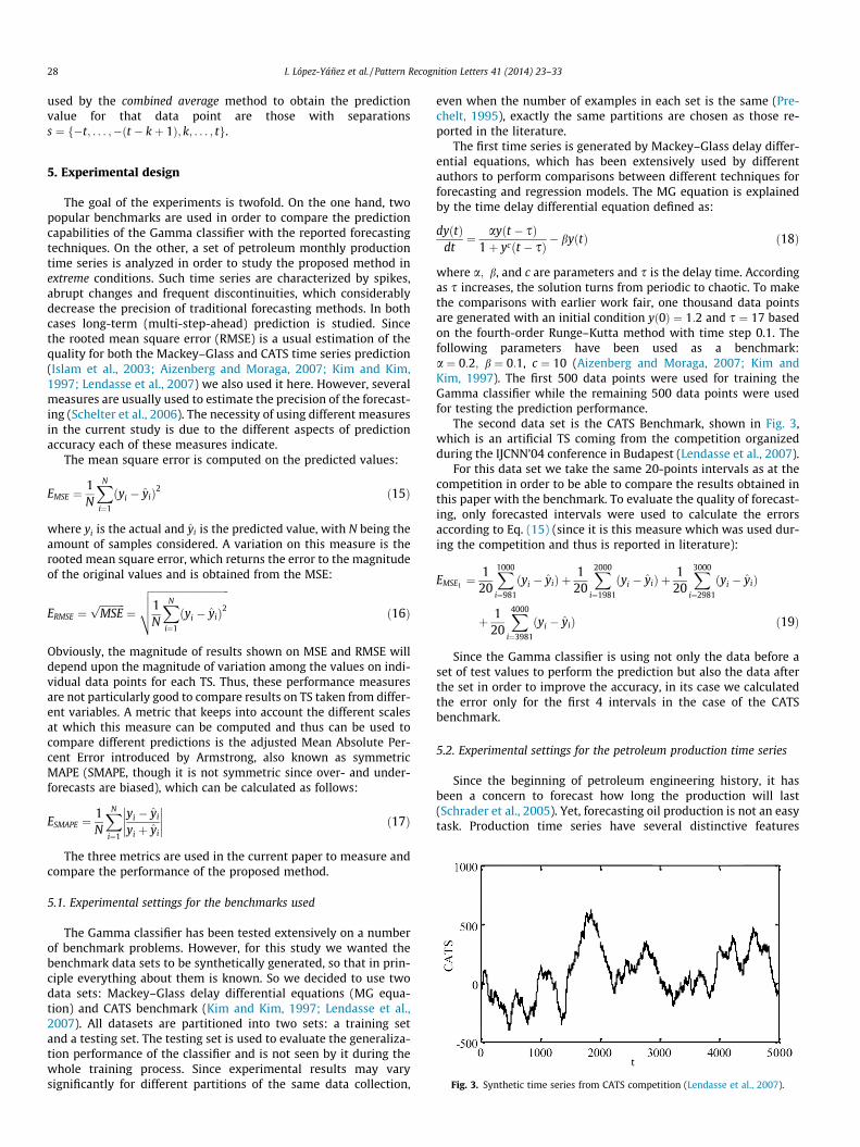
Fig. 3. Synthetic time series from CATS competition (Lendasse et al., 2007).

5. Experimental design

The goal of the experiments is twofold. On the one hand, twopopular benchmarks are used in order to compare the predictioncapabilities of the Gamma classifier with the reported forecastingtechniques. On the other, a set of petroleum monthly productiontime series is analyzed in order to study the proposed method inextreme conditions. Such time series are characterized by spikes,abrupt changes and frequent discontinuities, which considerablydecrease the precision of traditional forecasting methods. In bothcases long-term (multi-step-ahead) prediction is studied. Sincethe rooted mean square error (RMSE) is a usual estimation of thequality for both the Mackey–Glass and CATS time series prediction(Islam et al., 2003; Aizenberg and Moraga, 2007; Kim and Kim,1997; Lendasse et al., 2007) we also used it here. However, severalmeasures are usually used to estimate the precision of the forecast-ing (Schelter et al., 2006). The necessity of using different measuresin the current study is due to the different aspects of predictionaccuracy each of these measures indicate.

The mean square error is computed on the predicted values:

EMSE ¼1N

XN

i¼1

yi � yið Þ2 ð15Þ

where yi is the actual and yi is the predicted value, with N being theamount of samples considered. A variation on this measure is therooted mean square error, which returns the error to the magnitudeof the original values and is obtained from the MSE:

ERMSE ¼ffiffiffiffiffiffiffiffiffiffiMSEp

¼

ffiffiffiffiffiffiffiffiffiffiffiffiffiffiffiffiffiffiffiffiffiffiffiffiffiffiffiffiffiffiffi1N

XN

i¼1

yi � yið Þ2vuut ð16Þ

Obviously, the magnitude of results shown on MSE and RMSE willdepend upon the magnitude of variation among the values on indi-vidual data points for each TS. Thus, these performance measuresare not particularly good to compare results on TS taken from differ-ent variables. A metric that keeps into account the different scalesat which this measure can be computed and thus can be used tocompare different predictions is the adjusted Mean Absolute Per-cent Error introduced by Armstrong, also known as symmetricMAPE (SMAPE, though it is not symmetric since over- and under-forecasts are biased), which can be calculated as follows:

ESMAPE ¼1N

XN

i¼1

yi � yi

yi þ yi

�������� ð17Þ

The three metrics are used in the current paper to measure andcompare the performance of the proposed method.

5.1. Experimental settings for the benchmarks used

The Gamma classifier has been tested extensively on a numberof benchmark problems. However, for this study we wanted thebenchmark data sets to be synthetically generated, so that in prin-ciple everything about them is known. So we decided to use twodata sets: Mackey–Glass delay differential equations (MG equa-tion) and CATS benchmark (Kim and Kim, 1997; Lendasse et al.,2007). All datasets are partitioned into two sets: a training setand a testing set. The testing set is used to evaluate the generaliza-tion performance of the classifier and is not seen by it during thewhole training process. Since experimental results may varysignificantly for different partitions of the same data collection,

even when the number of examples in each set is the same (Pre-chelt, 1995), exactly the same partitions are chosen as those re-ported in the literature.

The first time series is generated by Mackey–Glass delay differ-ential equations, which has been extensively used by differentauthors to perform comparisons between different techniques forforecasting and regression models. The MG equation is explainedby the time delay differential equation defined as:

dyðtÞdt¼ ayðt � sÞ

1þ ycðt � sÞ � byðtÞ ð18Þ

where a; b, and c are parameters and s is the delay time. Accordingas s increases, the solution turns from periodic to chaotic. To makethe comparisons with earlier work fair, one thousand data pointsare generated with an initial condition yð0Þ ¼ 1:2 and s ¼ 17 basedon the fourth-order Runge–Kutta method with time step 0.1. Thefollowing parameters have been used as a benchmark:a ¼ 0:2; b ¼ 0:1, c ¼ 10 (Aizenberg and Moraga, 2007; Kim andKim, 1997). The first 500 data points were used for training theGamma classifier while the remaining 500 data points were usedfor testing the prediction performance.

The second data set is the CATS Benchmark, shown in Fig. 3,which is an artificial TS coming from the competition organizedduring the IJCNN’04 conference in Budapest (Lendasse et al., 2007).

For this data set we take the same 20-points intervals as at thecompetition in order to be able to compare the results obtained inthis paper with the benchmark. To evaluate the quality of forecast-ing, only forecasted intervals were used to calculate the errorsaccording to Eq. (15) (since it is this measure which was used dur-ing the competition and thus is reported in literature):

EMSE1 ¼1

20

X1000

i¼981

yi � yið Þ þ 120

X2000

i¼1981

yi � yið Þ þ 120

X3000

i¼2981

yi � yið Þ

þ 120

X4000

i¼3981

yi � yið Þ ð19Þ

Since the Gamma classifier is using not only the data before aset of test values to perform the prediction but also the data afterthe set in order to improve the accuracy, in its case we calculatedthe error only for the first 4 intervals in the case of the CATSbenchmark.

5.2. Experimental settings for the petroleum production time series

Since the beginning of petroleum engineering history, it hasbeen a concern to forecast how long the production will last(Schrader et al., 2005). Yet, forecasting oil production is not an easytask. Production time series have several distinctive features

Table 2Statistic characteristics of the 6 selected time series.

Characteristic TS 1 TS 2 TS 3

Data points 154 296 126Linear trend �264:52xþ 79625 N/A �84:437xþ 89559

R2 0.27 N/A 0.02

Mean 59,366.91 46,083.38 84,440.67Std. deviation 24,245.14 50,872.73 21,880.89Mode 86,185.58 14,819.24 97,495.00Skewness �0.81 1.11 �0.58Kurtosis �0.34 �0.31 2.64

TS 4 TS 5 TS 6

Data points 131 139 140Linear �0:0927x �645:83x �763:69xtrend +9590.6 +96228 +111875

R2 0.00 0.67 0.43

Mean 6,692.23 58,381.15 55,221.67Std. deviation 2,118.10 29,912.79 45,683.36Mode 6,824.65 81,493.00 72,007.00Skewness 0.57 �0.14 0.68Kurtosis 1.67 �1.07 �0.10

I. López-Yáñez et al. / Pattern Recognition Letters 41 (2014) 23–33 29

regarding their predictability, which separate them from financialTS or physical processes TS, which are usually used for forecastingcompetitions.

On the plot shown in Fig. 4, production TS of two wells are pre-sented for a typical brown oilfield of 25-years history. First,monthly production TS are rather short, the longest one has about300 data points; the rest of the series will be shorter covering onlyseveral years or even months of production, so the data sets mayonly be a few dozens points long. Moreover, many TS are discontin-uous (series 2): there are periods when for some reason the well isshut. Usually, a data set is predictable on the shortest time scales,but has global events that are harder to predict (spikes). Theseevents can be caused by workovers, change of producing intervalsand formations and so on. As a consequence, the data sets havehigh-dimensional dynamics and different trends.

As can be seen, such TS lack typical patterns such as periodicity,seasonality, or cycles. Even though direct measurements are possi-ble, the sampling process for these data is considered noisy. Thus,we are also interested in identifying data that deviates from the ex-pected patterns of the series, which may be caused by eventsknown or unknown a priori. The detection of abrupt changes in sig-nals is a classical problem in signal processing (Pollock, 1999).However, current change detection methods tend to be quitesophisticated in nature (e.g. Bayesian approach which requiresestimates of the a priori probabilities).

For the oil production experiments a data set consisting of 6randomly selected TS was used. Table 2 summarize statistic char-acteristics of the selected TS. Forecasting of the production TS isusually made on a one-year basis. Though the selected data setcovered in all cases more than 10 years periods, discontinuitiesfound almost in all TS (e.g. series 2 in Fig. 4), substantially reducedthe training basis.

Former studies on forecasting oil production (Schrader et al.,2005; González et al., 2012; Menezes and Barreto, 2008) haveproved the feasibility of ANN application. Though NARX architec-tures have been very effective for long-term temporal dependen-cies, on the selected data set the NARX model did not show goodresults, apparently due to the effects of discontinuities in the TS.This issue was a strong motivation to study and further developalternative forecasting techniques.

6. Experimental results

In order to test the proposed prediction model, it was applied tothe Mackey–Glass and CATS benchmarks TS, as well as to severalTS related to oil production, which were previously described.

6.1. Mackey–Glass benchmark

For this experiment, the TS data was generated for s ¼ 17,taking only the segment from time ¼ 124 to time ¼ 1123 into

Fig. 4. Example of monthly well oil production time series: (1) spike, (2) abruptchange, (3) discontinuity and (4) different trend segments.

consideration. From these 1000 samples, the first 500 were usedfor training and the latter 500 points were used for testing.Although a long term prediction under the former conditions isfeasable for the proposed model (thanks to the inclusion of the sep-aration concept), such experimental setting would require a quitelarge number of Gamma classifiers to be trained. Thus, test inputpatterns were built with samples taken both from the trainingand testing portions of the TS, but without learning from the latter.Other important parameters used for this experiment were thelength of the segments used to build the input patterns, n ¼ 10,and the length of the prediction period—which was moved throughthe testing portion of the TS as a sliding window—t ¼ 10. Thus, inorder to compute the predicted value at a specific point, all Gammaclassifiers with varying values for s ¼ 1;2; . . . ; t were prompted andthe resulting values were integrated using the Combined averagescheme.

In order to assess the results obtained, RMSE was used giventhat it is the performance measure of choice for this TS throughthe consulted literature, obtaining a RMSE of 0.0015. Table 3 in-cludes a comparison against other models (Kim and Kim, 1997;Aizenberg and Moraga, 2007).

As can be seen, the proposed model based on the Gamma clas-sifier clearly outperforms the other techniques, giving an RMSEwhich is approximately four times smaller than that of GEFREX(0.0015 against 0.0061), its closest competition.

6.2. CATS benchmark

For this benchmark TS, the testing periods are already defined:there are five segments 20 samples long each, thus having the

Table 3Comparison of performance on the Mackey–Glass benchmark (Aizenberg and Moraga,2007; Kim and Kim, 1997). Items in bold indicate best performances.

Model RMSE

Proposed model 0.0015MLMVN 0.0063CNNE 0.0090SuPFuNIS 0.0140GEFREX 0.0061EPNet 0.0200GFPE 0.0260Classical BP NN 0.0200ANFIS 0.0074

Table 5Experimental results for mean square error in millions (MSE � 1.0E+06) andsymmetric mean absolute percentage error in percentages (SMAPE). Items in boldindicate best performances.

Time series Combined Combined avg.

n ¼ 12 n ¼ 18 n ¼ 24 n ¼ 12 n ¼ 18 n ¼ 24

Mean squared errorTS 1 24.01 27.50 28.82 20.87 20.96 36.08TS 2 33.76 38.11 105.28 48.39 64.32 60.49TS 3 8.71 20.30 35.59 8.71 28.78 36.55TS 4 0.99 3.43 4.06 1.19 2.60 5.62TS 5 297.13 195.10 206.62 297.13 291.22 202.31TS 6 28.05 64.07 4.12 29.48 82.83 15.08

Symmetric mean absolute percentage errorTS 1 3.04% 3.49% 3.23% 3.04% 2.72% 3.66%TS 2 22.52% 31.72% 29.08% 31.62% 31.72% 29.08%TS 3 1.82% 2.48% 2.84% 1.82% 2.64% 3.28%TS 4 5.08% 13.76% 10.46% 4.88% 11.40% 16.09%TS 5 18.58% 13.21% 13.34% 18.58% 16.99% 12.15%TS 6 43.29% 38.93% 7.11% 36.16% 35.74% 15.16%

30 I. López-Yáñez et al. / Pattern Recognition Letters 41 (2014) 23–33

parameter s vary from 1 to t ¼ 20. Also, based on preliminary tests,the length for the input patterns was fixed at n ¼ 10, and the Com-bined average scheme was employed.

This TS was tested with three different models: the proposalpresented here as well as NARX and the classical Box–Jenkins AR-IMA (Box et al., 1994), and later compared to the published resultsof the CATS competition (Lendasse et al., 2007). For the first threemodels, the error measures considered before are used: MSE,RMSE, and SMAPE. In the case of the competition results, SMAPEis not reported and thus is not included in the comparison. The re-sults are shown in Table 4.

Again, the proposed model outperforms previous techniques. Inthe case of ARIMA, the MSE is almost 10 times smaller, while boththe MSE and RMSE for the Gamma classifier predictor are lowerthan the winners of the CATS competition.

An aspect worth notice is that the performance of the NARXmodel was better than that of ARIMA for both MSE (aproximately1=3) and RMSE, yet its corresponding SMAPE is almost three timesthat of ARIMA. Indeed, this behavior where a particular method of-fers good performance on one metric but a lesser one on anothermetric has emerged several times in our experiments. While anin-depth study related to this phenomenon is out of the scope ofthe present paper, this apparently inconsistent performance seemsto be related to how different performance metrics emphasize dif-ferent aspects of the errors. For instance, a particular metric couldgive more weight to large errors than to small ones, while anothermetric could make errors done on large original values more costlythan those corresponding to small original values. As was men-tioned previously, this is the reason why several performance mea-sures are used in this paper.

6.3. Oil production

Three scenarios were considered, with input segments of lengthn ¼ 12; n ¼ 18, and n ¼ 24 samples, in order to find out how thelength of the input patterns affects prediction. On the other hand,both the Combined and Combined average schemes were used, vary-ing s ¼ 1;2; . . . ;12 in order to compute each data point in the pre-diction segment, which is one year long. Performance wasevaluated using MSE and SMAPE. The results are summarized inTable 5, while the resulting predictions are shown in Fig. 5.

As can be seen, the performance of the proposed method variesthroughout the different experiments, as was expected given thedifferences presented by the TS used. TS 1 and 3 show very goodresults on both metrics, while TS 4 has very good MSE and reason-ably good SMAPE. On the other hand, the errors for TS 5 are largefor both metrics.

Now, when we turn to the plots, the reasons for such behaviorsstart to emerge. Both TS 1 and 3 have no discontinuities, while TS 4presents only one. The other three TS, however, are riddled withdiscontinuities; for instance: out of the 296 samples of TS 2, only146 are valid data points grouped in five segments. Under suchconditions, it can only be expected that any predictors will havea hard time giving good results.

Table 4Comparison of performance on the CATS benchmark (Lendasse et al., 2007). Items inbold indicate best performances.

Model MSE RMSE SMAPE

Proposed model 163.9 12.79 4%ARIMA 1473.2 38.38 18%NARX 515.3 22.70 57%Ensemble models 222 14.90 –Fuzzy inductive reasoning 278 16.67 –Kalman smoother 346 18.60 –

It is noteworthy that for all six TS, on both variants (Combinedand Combined average) and both performance metrics, the best re-sults were obtained with test segments of length n ¼ 12. It is awell-known fact in TS forecasting that the farther away from thelearning samples, the greater the uncertainty in the prediction(Pollock, 1999; Schelter et al., 2006). However, given the character-istics and properties of the Gamma classifier—i.e. a segment and asample with arbitrary separation could be associated and learned—the effect of n was previously unknown.

In this sense, it is important to remark that determining theoptimal value of n for a given problem (i.e. a given TS) is still anopen problem. One way to address this circumstance in practice,particularly in the area of ANNs, is to use the autocorreletion toestimate the length of TS segments used as input to the network(variable n, the size of the input patterns, for the Gamma classifier).Although the value found varies from one TS to another, the con-sensus among the six TS used was a segment length of n < 30. Tak-ing into consideration that, in petroleum industry practice, theusual periods are multiples of six months, three length values wereselected to be experimented on, as was mentioned before:n ¼ 12; n ¼ 18, and n ¼ 24. As the experimental results show,n ¼ 12 tends to be a good bet for these six oil production TS.

Another interesting finding is that some TS offer quite good re-sults under some performance metrics, while the results for othermetrics are surprisingly poor. Such is the case of TS 6, whose MSE(1.51E+07 best, 3.73E+07 average) is below the mean of the six TS(6.61E+07), while its SMAPE (29.40% average, 43.29% worst) is con-siderably above the mean (15.02%, respectively).

As mentioned previously, each metric emphasizes different as-pects of the prediction error, thus giving rise to such apparent dis-crepancies. What remains to be found is why such largeinconsistencies in performance arise.

For comparison purposes, two TS were tested using ARIMA: TS 1and TS 2. These results are shown in Table 6, considering that theresults of the proposed method are those when n ¼ 12 and theCombined average scheme were used. As can be seen, the proposedmethod offers better results than ARIMA for both TS and both met-rics, even when the performance for TS 2 is considerably worsethan that for TS 1.

Table 6 also shows a comparison done on another oil produc-tion TS taken from the same oilfield (denoted as TS 7), consideringARIMA, six variants of ANN, and the Gamma classifier model, againwith n ¼ 12 and the Combined average scheme (Sheremetov et al.,2013). Once again, the performance of the proposed model is quitecompetitive: it has the lowest MSE (1.87E+08 against 2.16E+08 by

Fig. 5. Prediction of monthly oil production for six TS: (a) TS 1, (b) TS 2, (c) TS 3, (d) TS 4, (e) TS 5 and (f) TS 6.

I. López-Yáñez et al. / Pattern Recognition Letters 41 (2014) 23–33 31

ARIMA) and the lowest SMAPE, in a tie with ARIMA at 3%. As wasmentioned at the end of Section 5.2, the poor performance exhib-ited by some models of ANN in some of these TS motivated thedevelopment and application of the Gamma classifier to these fore-casting problems.

Another aspect worth mentioning is the concept of negativeseparations. Although using this concept, it is now possible to

predict test data points using future known values to build the cor-responding input patterns, this was not used in the previous exper-iments to predict the test segments. The negative values ofseparation were used only to reconstruct each TS (i.e. predictingthe known portions of each TS), emphazising the ability of theGamma classifier to correctly classify all known associations. Thisis important in the context of missing values and discontinuities,

Table 6Performance comparison for time series TS 1, TS 2, and TS 7 (Sheremetov et al., 2013) (in MSE � 1.0E+06 and SMAPE). Items in bold indicate best performances.

Method TS 7 TS 1 TS 2

MSE SMAPE MSE SMAPE MSE SMAPE

Gamma-based 187 3% 20.87 3.04% 48.39 31.62%model ARIMA 216 3% 131.07 7.81% 174.31 39.59%NARX (Log-Tan multi) 248 6% – – – –NARX (Tan-Lin multi) 1070 10% - - – –NARX (Tan-Tan) 417 7% – - – –NARX (Log-Tan) 377 8% – – – –TDNN (Log-Tan) 904 13% – – – –TDNN (Tan-Lin) 2570 17% – – – –

32 I. López-Yáñez et al. / Pattern Recognition Letters 41 (2014) 23–33

especially considering that most other methods which have beentested on the selected TS have given some error on thisreconstruction.

Again, since the focus of these experiments was the test seg-ments, no comparisons were done on the known segments of eachTS, and thus the effects of negative separations are not evidencedin these experimental results. Also, the task of prediction for oilproduction TS is rather interested on future values, making theuse of negative separations to predict test segment valuesunadvisable.

7. Discussion and conclusions

In this paper the forecasting capabilities of an associative modelare studied. The main result is that a novel non-linear forecastingtechnique based on the Gamma classifier associative model isintroduced. Its performance for long-term time horizons both onforecasting benchmarks and a specific data set of oil wells monthlyproduction was tested. The Gamma classifier model outperformedpreviously reported techniques in terms of forecast accuracy.

This is not an easy achievement, considering that the predictiontask is reformulated as a supervised classification task. Althoughother methods employ supervised learning to solve this problem,none of those against which the Gamma classifier model was com-pared do so from a classification perspective. Also, as mentionedpreviously, several Pattern Recognition, Machine Learning or Com-putational Inteligence models are used for the task of TS classifica-tion, but such methods have seen little application in theforecasting area.

In this sense, the forecasting algorithm used by ANN in the caseof multi-step-ahead or long-term prediction differs substantiallyfrom that of the Gamma classifier. For the former case, the modelsoutput is fed back to the input regressor for a finite number of timesteps. Thus, the components of the input regressor, previouslycomposed of actual sample points of the TS, are gradually replacedby previous predicted values. For very long-term prediction, even-tually, the multi-step-ahead prediction task becomes a dynamicmodeling task, in which the neural network model acts as anautonomous system, trying to recursively emulate the dynamicbehavior of the system that generated the nonlinear TS (Aceve-do-Mosqueda et al., 2007).

On the other hand, a similar strategy of pattern definition asused in this paper, was applied by Zhang and Hutchison (Zhangand Hutchinson, 1994) who also used the differences betweentwo neighboring points. But they were interested in predictingwhich direction a financial TS was headed rather than to attemptto predict the exact value of the TS. Thus these differences werecoded as one of three values: increasing (þ), decreasing (�), orno change (0), depending on whether the differences were positive,negative, or (close to) zero. These coded differences were then usedas inputs to multilayer perceptron networks.

Moreover, the proposed method uses only one variable whenthere are more available, and the phenomena under study are con-sidered to be rather complex. Experiments with the Gamma classi-fier-based predictor under multivariate settings for oil productionforecasting are on-going.

On a different track, the dependencies of forecasting uncer-tainty on separation between predicted data point and known datahave been confirmed, despite the independency offered by the pro-posed model. This indicates a likely dependency in the actual datasampled from the natural phenomenon, which remains to betested. Additionally, the pernicious effects of discontinuities inthe TS data were confirmed for this method, even though it worksunder more extreme conditions than the classical approaches, evenoffering competitive performances.

Additionally, these experimental results and their analysiscould very well serve as precursors for a more extensive character-ization of TS based on the properties and performances obtained bycombinations of the proposed forecasting model and different met-rics. Such efforts are currently under development.

There are two remaining open problems, which were men-tioned in this paper. On one hand, we have the issue of determin-ing the optimal value for n given a specific problem or TS, and theforecasting method to be used. On the other hand, the phenome-non of a method giving good results on one performance metricand bad results on another has not been fully studied. Finally,the relationship between the Gamma operator (and hence theGamma classifier) and the Hamming distance opens a new venuefor research.

Acknowledgments

This research was partially supported by the CONACYT-SENER(project 146515), as well as the Instituto Politécnico Nacional (Sec-retaría Académica, COFAA, SIP, CIDETEC and CIC), CONACyT, andSNI.

References

Acevedo-Mosqueda, M.E., Yáñez-Márquez, C., López-Yáñez, I., 2007. Alpha–betabidirectional associative memories: theory and applications. Neural Process.Lett. 26 (1), 1–40.

Agrawal, R., Psaila, G., Wimmers, E.L., Zait, M., 1995. Querying shapes of histories.In: Proc. VLDB 1995, Zurich, Switzerland, pp. 502–514.

Aizenberg, I., Moraga, C., 2007. Multilayer feedforward neural network based onmulti-valued neurons (MLMVN) and a backpropagation learning algorithm. SoftComput. 11, 169–183.

Baldwin, J.F., Martin, T.P., Rossiter, J.M., 1998. Time series modeling and predictionusing fuzzy trend information. In: Proc. Int. Conf. SC Information/IntelligentSyst., pp. 499–502.

Batyrshin, I., Sheremetov, L., 2008. Perception based approach to time series datamining. J. Appl. Soft Comput. Sci. 8 (3), 1211–1221.

Bowerman, B.L., O’Connell, R.T., 1979. Time Series and Forecasting: An AppliedApproach. Mass Duxbury Press.

Box, G., Jenkins, G.M., Reinsel, G., 1994. Time Series Analysis: Forecasting & Control,third ed. Prentice Hall.

I. López-Yáñez et al. / Pattern Recognition Letters 41 (2014) 23–33 33

Cellier, F., Nebot, A., Mugica, F., De Albornoz, A., 1996. Combined qualitative/quantitative models of continuos-time processes using fuzzy inductivereasoning techniques. Int. J. Gen. Syst. 24, 95–106.

Cheung, J.T., Stephanopoulos, G., 1990. Representation of process trends. Part I: Aformal representation framework. Comput. Chem. Eng. 14, 495–510.

Cipra, T., Hanzak, T., 2011. Exponential smoothing for time series with outliers.Kybernetika 47 (2), 165–178.

Cohen, P., Adams, N., 2001. An algorithm for segmenting categorical time series intomeaningful episodes. In: Proc. Fourth International Symposium on IntelligentData Analysis, Lisbon, Portugal.

Das, G., Lin, K.I., Mannila, H., Renganathan, G., Smyth, P., 1998. Rule discovery fromtime series. In: Proc. KDD98, pp. 16–22.

De Gooijer, J.G., Hyndman, R.J., 2006. 25 Years of time series forecasting. Int. J.Forecast. 22, 443–473.

Fetkovich, M.J., 1987. Decline-curve analysis using type curves-case histories. SPEForm. Eval. 637.

González, A., Vargas, F., Cosultchi, A., 2012. Effect of treatments on oil wellproduction by ANN. In: Sheremetov, L., Haasis, H.-D., Villa-Vargas, L. (Eds.),Operations Research and Data Mining, ORADM 2012, Workshop Proceedings,IPN, pp. 261–269.

Hand, D., Manilla, H., Smyth, P., 2001. Principles of Data Mining. MIT Press,Cambridge.

Islam, M.M., Yao, X., Murase, K., 2003. A constructive algorithm for trainingcooperative neural network ensembles. IEEE Trans. Neural Networks 14 (4).

Jang, J.-S.R., 1993. ANFIS: adaptive-network-based fuzzy inference system. IEEETrans. Syst. Man Cybern. 23, 665–685.

Khazaeni, Y., Mohaghegh, S.D., 2010. Intelligent time successive productionmodeling. In: SPE 132643, Presented at the SPE Western Regional Meetingheld in Anaheim, California, 27–29 May 2010. Society of Petroleum Engineers.

Kim, D., Kim, C., 1997. Forecasting time series with genetic fuzzy predictorensemble. IEEE Trans. Fuzzy Syst. 5 (4), 523–535.

Landassuri-Moreno, V., Bullinaria, J.A., 2009. Neural network ensembles for timeseries forecasting. In: GECCO’09, July 8–12, 2009. ACM, Montral Qubec, Canada.

Lendasse, A., Oja, E., Simula, O., Verleysen, M., 2007. Time series predictioncompetition: the CATS benchmark (editorial). Neurocomputing 70, 2325–2329.

López-Yáñez, I., Argüelles-Cruz, A.J., Camacho-Nieto, O., Yáñez-Márquez, C., 2011.Pollutants time-series prediction using the Gamma classifier. Int. J. Comput.Intell. Syst. 4 (4), 680–711.

Menezes, J.M.P., Barreto, G.A., 2008. Long-term time series prediction with theNARX network: an empirical evaluation. Neurocomputing 71 (16–18), 3335–3343.

Mitra, S., Pal, S.K., Mitra, P., 2002. Data mining in soft computing framework: asurvey. IEEE Trans. Neural Networks 13 (1), 3–14.

Mohaghegh, S.D., 2005. Recent developments in application of artificial intelligencein petroleum engineering. J. Pet. Technol., Distinguished Author Ser., 86–91.

Palit, A.K., Popovic, D., 2005. Computational Intelligence in Time Series Forecasting.Springer-Verlag, London, UK.

Paul, S., Kumar, S., 2002. Subsethood-product fuzzy neural inference system(SuPFuNIS). IEEE Trans. Neural Networks 13 (3), 578–599.

Piao, M., Lee, H.G., Park, J.H., Ryu, K.H., 2008. Application of Classification Methodsfor Forecasting Mid-Term Power Load Patterns. Communications in Computerand Information Science, vol. 15. Springer, pp. 47–54.

Pollock, D.S.G., 1999. A Handbook of Time-Series Analysis, Signal Processing andDynamics. Academic Press, London, UK.

Prechelt, L., 1995. Some notes on neural learning algorithm benchmarking.Neurocomputing 9, 343–347.

Russo, M., 2000. Genetic fuzzy learning. IEEE Trans. Evol. Comput. 4, 259–273.Sarkka, S., Vehtari, A., Lampinen, J., 2004. Time series prediction by Kalman

smoother with cross validated noise density. In: IJCNN 04, Budapest.Schelter, B., Winterhalder, M., Timmer, J. (Eds.), 2006. Handbook of Time Series

Analysis. Wiley, Weinheim, Germany.Schrader, S.M., Balch R.S., Ruan T., 2005. Using neural networks to estimate monthly

production: a case study for the devonian carbonates, In: SPE ProductionOperations Symposium, 16–19 April 2005, SPE 94089, Southeast New Mexico,Oklahoma City, Oklahoma.

Sheremetov, L., Alvarado, M., Bañares-Alcántara, R., Anminzadeh, F., 2005.Intelligent computing in petroleum engineering (editorial). J. Pet. Sci. Eng. 47(1–2), 1–3.

Sheremetov, L., Haasis, H.-D., Villa-Vargas, L. (Eds.), 2012. Operations Research andData Mining, ORADM 2012, Workshop Proceedings, IPN, Mexico-city.

Sheremetov, L.B., González-Sánchez, A., López-Yáñez, I., Ponomarev, A.V., 2013.Time series forecasting: applications to the upstream oil and gas supply chain.In: IFAC MIM 2013, Saint Petersburg.

Sonrexa, K., Kumar, P.S., Al-Ajmi, H., 1997. Analytic technique to forecast productionfor non-declining oil wells in bounded solution-gas-drive reservoirs. SPE.

Sripada, S.G., Reiter, E., Hunter, J., Yu, J., 2002. Segmenting time series for weatherforecasting. In: Proc. ES2002, pp. 193–206.

van Golf-Racht, T.D., 1982. Fundamentals of Fractured Reservoir Engineering.Developments in Petroleum Science, vol. 12. Elsevier, Amsterdam, TheNetherlands.

Weiss, W.W., Balch, R.S., Stubbs, B.A., 2002. How artificial intelligence methods canforecast oil production. In: SPE 75143, presented in SPE/DOE Improved OilRecovery Symposium, Tulsa, Oklahoma 13–17 April 2002.

Wichard, J., Ogorzalek, M., 2004. Time series prediction with ensemble models. In:IJCNN 04, Budapest.

Yáñez-Márquez, C., Felipe-Riverón, E.M., López-Yáñez, I., Flores-Carapia, R., 2006. ANovel Approach to Automatic Color Matching. Lecture Notes in ComputerScience, LNCS, vol. 4225. Springer-Verlag, Berlin, Heidelberg, pp. 529–538.

Yao, X., Liu, Y., 1997. A new evolutionary system for evolving artificial neuralnetworks. IEEE Trans. Neural Networks 8, 694–713.

Zhang, X., Hutchinson, J., 1994. Simple architectures on fast machines: practicalissues in nonlinear time series prediction. In: Time Series Prediction,Forecasting the Future and Understanding the Past. Addison-Wesley, Reading,MA, pp. 1–70.