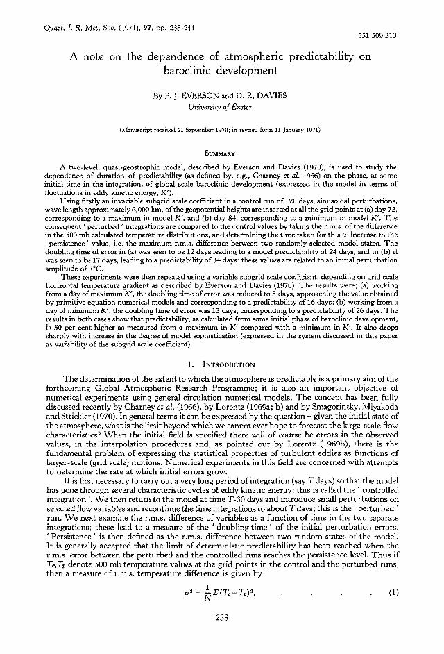
Quart. J . R. Met. SOC. (1971), 97, pp. 238-241 551.509.313

A note on the dependence of atmospheric predictability on baroclinic development

By P. J. EVERSON and D. R. DAVIES University of Exeter

(Manuscript received 21 September 1970; in revised form 11 January 1971)

SUMMARY

A two-level, quasi-geostrophic model, described by Everson and Davies (1970), is used to study the dependence of duration of predictability (as defined by, e.g., Charney et al. 1966) on the phase, at some initial time in the integration, of global scale baroclinic development (expressed in the model in terms of fluctuations in eddy kinetic energy, K').

Using firstly an invariable subgrid scale coefficient in a control run of 120 days, sinusoidal perturbations, wave length approximately 6,000 km, of the geopotential heights are inserted at all the grid points at (a) day 72, corresponding to a maximum in model K', and (b) day 84, corresponding to a minimum in model K'. The consequent ' perturbed ' integrations are compared to the control values by taking the r.m.s. of the difference in the 500 mb calculated temperature distributions, and determining the time taken for this to increase to the ' persistence ' value, i.e. the maximum r.m.s. difference between two randomly selected model states. The doubling time of error in (a) was seen to be 12 days leading to a model predictability of 24 days, and in (b) it was seen to be 17 days, leading to a predictability of 34 days: these values are related to an initial perturbation amplitude of 1°C.

These experiments were then repeated using a variable subgrid scale coefficient, depending on grid scale horizontal temperature gradient as described by Everson and Davies (1970). The results were; (a) working from a day of maximum K', the doubling time of error was reduced to 8 days, approaching the value obtained by primitive equation numerical models and corresponding to a predictability of 16 days; (b) working from a day of minimum K', the doubling time of error was 13 days, corresponding to a predictability of 26 days. The results in both cases show that predictability, as calculated from some initial phase of baroclinic development, is 50 per cent higher as measured from a maximum in K' compared with a minimum in K'. It also drops sharply with increase in the degree of model sophistication (expressed in the system discussed in this paper as variability of the subgrid scale coefficient).

1. INTRODUCTION

The determination of the extent to which the atmosphere is predictable is a primary aim of the forthcoming Global Atmospheric Research Programme; it is also a n important objective of numerical experiments using general circulation numerical models. T h e concept has been fully discussed recently by Charney et al. (1966), by Lorentz (1969a; b ) and by Smagorinsky, Miyakoda and Strickler (1970). In general terms it can be expressed by the question - given the initial state of the atmosphere, what is the limit beyond which we cannot ever hope to forecast the large-scale flow characteristics? When the initial field is specified there will of course be errors in the observed values, in the interpolation procedures and, as pointed out by Lorentz (1969b), there is the fundamental problem of expressing the statistical properties of turbulent eddies as functions of larger-scale (grid scale) motions. Numerical experiments in this field are concerned with attempts t o determine the rate a t which initial errors grow.

It is first necessary to carry out a very long period of integration (say T days) so that the model has gone through several characteristic cycles of eddy kinetic energy; this is called the ' controlled integration I . We then return t o the model at time T-30 days and introduce small perturbations on selected flow variables and recontinue the time integrations to about T days; this is the ' perturbed ' run. W e next examine the r.m.s. difference of variables as a function of time in the two separate integrations; these lead t o a measure of the ' doubling time ' of the initial perturbation errors. ' Persistence ' is then defined as the r.m.s. difference between two random states of the model. It is generally accepted that the limit of deterministic predictability has been reached when the r.m.s. error between the perturbed and the controlled runs reaches the persistence level. Thus if T,,T, denote 500 m b temperature values a t the grid points in t h e control and the perturbed runs, then a measure of r.m.s. temperature difference is given by

(1) 1 N U* = -L'(Tc-Tp)*,

238

SHORTER CONTRIBUTIONS 239

where N is the total number of grid points and the summation is over these. A convenient method of determining persistence is then obtained by replacing Tp by the distribution of initial Tc values.

Early values, using e.g. the Mintz-Arakawa primitive equation model (see Charney et al. 1966), gave a 5 day doubling time and a predictability of 15 days. The possible influence of initial conditions was not considered. However, some numerical experiments by Davies and Davies (1969) clearly demonstrated that the particular functional forms chosen for the initial distribution of disturbing stream function values, as used in many general circulation studies, strongly marked the flow patterns for at least thirty days of baroclinic development, and it was suggested that initial conditions could appreciably influence the calculated predictability. Recent work by Smagorinsky, Miyakoda and Strickler (1970), using their 9-level, primitive equation model, has shown that some surface meteorological variables are not really essential as initial data for the prediction of extra tropical cyclone scale flows for a few days ahead; this result could of course have a crucial bearing on the planning of GARP.

In considering the problem of the effect of initial conditions, practical experience strongly suggests that the limit of predictability depends on the phase of baroclinic development in the real atmosphere at the initial time considered. This suggests that numerical predictability experiments should be carried out with starting points at the maxima and minima of the model eddy kinetic energy curves, these points representing extreme points of model baroclinic development.

2. THE MODEL AND NUMERICAL RESULTS

The model used was that described recently by Everson and Davies (1970). This is a two-level quasi-geostrophic system with an Arakawa type of finite difference scheme; this model, although it is of comparatively simple structure, contains certain primary features of the general circulation. It has enabled us to study the importance of the cycle of global eddy kinetic energy in considerations of blocking anticyclonic systems and to examine the effects of two alternative subgrid scale formulations.

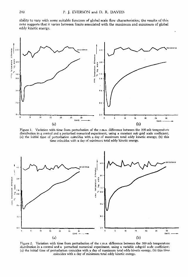
Using firstly a subgrid scale coefficient, which was assumed to be independent of spacial position and of time, a control run of 120 days was carried out. A sinusoidal perturbation in the geopotential heights was then inserted at all the grid points at (a) day 72 of the control run, corresponding to a maximum in the model eddy kinetic energy function, K'(t), and then at (b) day 84, corresponding to a minimum in K': the total disturbing effect was constrained to be equivalent to an initial r.m.s. temperature difference of 1°C. The consequent ' perturbed ' integrations are compared to the control values as a function of time by taking the r.m.s. difference of the 500 mb calculated temperature distributions, using Eq. (I), the value being 1°C at the initial time of perturbation. The value, as in all models, falls rapidly at first, but then after about day 2 it increases, as the baroclinic instabilities increase the initial error. The computed curves (together with the persistence calculation centred at about 4°C) are shown in Fig. l(a) and (b), and a comparison of the error in case (a), maximum K', at day 18 after perturbation with that at day 30 displays a doubling time of error of about 12 days, indicating a predictability period of about 24 days. The corresponding case (b), of minimum K', indicates a doubling time of error of about 17 days, leading to a predictability of about 34 days.

These numerical experiments were then repeated using a variable subgrid-scale coefficient, discussed by Everson and Davies (1970), depending on grid scale horizontal temperature gradient. It was in fact shown by Everson and Davies that, if we represent subgrid scale effects in the equations of motion by terms of the form AVZu, where u is the appropriate horizontal velocity component, and allow the coefficient A to vary with baroclinicity expressed as the mean of the magnitudes of temperature gradient on the grid scale in the meridional and zonal directions, then a more realistically behaved model was produced, The ' predictability ' results are shown in Fig. 2(a) and (b); in Fig. 2(a), working from a day of maximum K , day 87, the doubling time of error was now reduced to 8 days (approaching the value obtained by primitive equation numerical models), corresponding to a predictability of 16 days, and in Fig. 2(b), working from a day of minimum K , day 69, the doubling time of error was 13 days, corresponding to a predictability of 26 days.

The results obtained in both of these cases show that our model predictability, as calculated from some initial phase of baroclinic development, is 50 per cent higher, when measured from a day of minimum in K' compared with the result obtained when measured from a starting point at a maximum in K'. It is also seen that predictability drops sharply with increase in the degree of model sophistication (expressed in the system discussed in this paper as variability of the subgrid scale coefficient). We note finally that we would of course expect the real atmosphere's predict-

210 P. J. EVERSON and D. R. DAVIES

ability to vary with some suitable function of global scale flow characteristics; the results of this note suggests that it varies between limits associated with the maximum and minimum of global eddy kinetic energy.

persistence - Persistence w

0.1 5 10 0 5 10 15 30 20 25 15 20 25 30

DAYS - DAYS - (a) (b)

Figure 1. Variation with time from perturbation of the r.m.s. difference between the 500 mb temperature distribution in a control and a perturbed numerical experiment, using a constant sub grid scale coefficient; (a) the initial time of perturbation coincides with a day of maximum total eddy kinetic energy; (b) this

time coincides with a day of minimum total eddy kinetic energy.

0.1

G 5 1G 15 28 25 30 0 5 10 15 20 25 30 DAYS ____) D*YS -

(a) (b) Figure 2. Variation with time from perturbation of the r.m.s. difference between the 500 mb temperature distribution in a control and a perturbed numerical experiment, using a variable subgrid scale coefficient; (a) the initial time of perturbation coincides with a day of maximum total eddy kinetic energy, (b) this time

coincides with a day of minimum total eddy kinetic energy.

SHORTER CONTRIBUTIONS 241

ACKNOWLEDGMENT

One of the authors (PJE) gratefully acknowledges the award of a research studentship by NERC, enabling him to carry out these investigations.

REFERENCES Charney, J. G. and co-workers 1966 ‘ The feasibility of a global observation and analysis experi-

ment,’ Publication 1290, Nat. Acad. Sci; Nat. Res. Council, Washington, D.C.

‘Some numerical experiments using a two-level general circulation model,’ Quart. J. R. Met. Soc., 95, pp.

Davies, D. J. and Davies, D. R. 1969

148-162. Everson, P. J. and Davies, D. R. 1970 ‘ On the use of a simple two-level model in general circulation

studies,’ Ibid., 96, pp. 404-412.

motion,’ Tellus, 21, pp. 289-307.

Amer. Met. Soc., 50, p. 345-349.

Lorentz, E. N. 1969(a) ‘ The predictability of a flow which possesses many scales of

1969(b) Three approaches to atmospheric predictability,’ Bull.

1970 ‘ The relative importance of variables in initial conditions Strickler, R. F. for dynamical weather prediction,’ Tellus, 22, pp.

Smagorinsky, J., Miyakoda, K. and

141-157.