1

A Nonstochastic Information Theoryfor Communication and State Estimation

Girish N. Nair

Abstract—In communications, unknown variables are usuallymodelled as random variables, and concepts such as indepen-dence, entropy and information are defined in terms of theunderlying probability distributions. In contrast, control theoryoften treats uncertainties and disturbances as bounded unknownshaving no statistical structure. The area of networked controlcombines both fields, raising the question of whether it is possibleto construct meaningful analogues of stochastic concepts suchas independence, Markovness, entropy and information withoutassuming a probability space. This paper introduces a frameworkfor doing so, leading to the construction of a maximin informationfunctional for nonstochastic variables. It is shown that the largestmaximin information rate through a memoryless, error-pronechannel in this framework coincides with the block-coding zero-error capacity of the channel. Maximin information is then usedto derive tight conditions for uniformly estimating the state ofa linear time-invariant system over such a channel, parallelingrecent results of Matveev and Savkin.

Index Terms—Nonprobabilistic information theory, zero-errorcapacity, erroneous channel, state estimation.

I. INTRODUCTIONThis paper has two motivations. The first arises out of the

analysis of networked control systems [2], which combinethe two different disciplines of communications and control.In communications systems, unknown quantities are usuallymodelled as random variables (rv’s), and central conceptssuch as independence, Markovness, entropy and Shannoninformation are defined stochastically. One reason for this isthat they are generally prone to electronic circuit noise, whichobeys physical laws yielding well-defined distributions. Inaddition, communication systems are often used many times,and in everyday applications each phone call and data bytemay not be important. Consequently, the system designer needonly ensure good performance in an average or expected sense- e.g. small bit error rates and large signal-to-noise averagepower ratios.

In contrast, control is often used in safety- or mission-critical applications where performance must be guaranteedevery time a plant is used, not just on average. Furthermore,in plants that contain mechanical and chemical components,the dominant disturbances may not necessarily arise fromcircuit noise, and may not follow a well-defined probabilitydistribution. Consequently, control theory often treats uncer-tainties and disturbances as bounded unknowns or signalswithout statistical structure. Networked control thus raisesnatural questions of whether it is possible to construct useful

Published in IEEE Trans. Automatic Control, vol. 58, no. 6, pp. 1497–1510, 2013. This work was supported by Australian Research Councilgrant DP110102401. A preliminary version appeared in [1]. G.N. Nair iswith the Department of Electrical and Electronic Engineering, Universityof Melbourne, VIC 3010, Australia, tel: +61-3-8344-6701, fax: +61-3-8344-6678, email: gnair@unimelb.edu.au

analogues of the stochastic concepts mentioned above, withoutassuming a probability space.

Such questions are not new and some answers are available.For instance, if an rv has known range but unknown distribu-tion, then its uncertainty may be quantified by the logarithm ofthe cardinality or Lebesgue measure of this range. This leadsto the notions of Hartley entropy H0 [3] for discrete variablesand Renyi differential 0th-order entropy h0 [4] for continuousvariables. A related construction is the ε-entropy, which is thelog-cardinality of the smallest partition of a given metric spacesuch that each partition set has diameter no greater than ε > 0[5], [6], [7]. None of these concepts require any statisticalstructure.

Using these notions, nonstochastic measures of informationcan be constructed. For instance, in [8] the difference betweenthe marginal and worst-case conditional Renyi entropies wastaken to define a nonstochastic, asymmetric information func-tional, and used to study feedback control over errorless digitalchannels. In [9], information transmission was defined sym-metrically as the difference between the sum of the marginaland the joint Hartley entropies of a pair of discrete variables.Continuous variables with convex ranges admitted a similarconstruction, but with H0 replaced by a projection-based,isometry-invariant functional. Although both these definitionspossess many natural properties, their wider operational rele-vance is unclear. This contrasts with Shannon’s theory, whichis intimately connected to quantities of practical significancein engineering, such as the minimum and maximum bit-ratesfor reliable compression and transmission [10].

The second, seemingly unrelated motivation comes from thestudy of zero-error capacity C0 [11], [12] in communications.The zero-error capacity of a stochastic discrete channel is thelargest block-coding rate possible across it that ensures zeroprobability of decoding error. This is a more stringent conceptthan the (ordinary) capacity C [10], defined to be the highestblock-coding rate such that the probability of a decoding erroris arbitrarily small. The famous channel coding theorem [10]states that the capacity of a stochastic, memoryless channelcoincides with the highest rate of Shannon information acrossit, a purely intrinsic quantity. In [13], an analogous identityfor C0 was found in terms of the Shannon entropy of the‘largest’ rv common to the channel input and output. However,it is known that C0 does not depend on the values of thenon-zero transition probabilities in the channel and can bedefined without any reference to a probabilistic framework.This strongly suggests that C0 should be expressible as themaximum rate of a suitably defined nonstochastic informationindex.

This paper has four main contributions. In section II, aformal framework for modelling nonstochastic uncertain vari-

arX

iv:1

112.

3471

v5 [

cs.S

Y]

11

Jan

2014

2

ables (uv’s) is proposed, leading to analogues of probabilisticideas such as independence and Markov chains. In sectionIII, the concept of maximin information I∗ is introduced toquantify how much the uncertainty in one uv can be reducedby observing another. Two characterizations of I∗ are givenhere, and shown to be equivalent. In section IV, the notionof an error-prone, stationary memoryless channel is definedwithin the uv framework, and it is proved in Theorem 4.1that the zero-error capacity C0 of any such channel coincideswith the largest possible rate of maximin information acrossit. Finally, it is shown in section V how I∗ can be used tofind a tight condition (Theorem 5.1) that describes whetheror not the state of a noiseless linear time-invariant (LTI)system can be estimated with specified exponential uniformaccuracy over an erroneous channel. A tight criterion for theachievability of uniformly bounded estimation errors is alsoderived for when uniformly bounded additive disturbancesare present (Theorem 5.2); a similar result was derived in[14], using probability arguments but no information theory.In a nonstochastic setting, maximin information thus serves todelineate the limits of reliable communication and LTI stateestimation over error-prone channels.

II. UNCERTAIN VARIABLES

The key idea in the framework proposed here is to keep theprobabilistic convention of regarding an unknown variable as amapping X from some underlying sample space Ω to a set X ofinterest. For instance, in a dynamic system each sample ω ∈Ω

may be identified with a particular combination of initial statesand exogenous noise signals, and gives rise to a realizationX(ω) denoted by lower-case x ∈ X. Such a mapping X iscalled an uncertain variable (uv). As in probability theory, thedependence on ω is usually suppressed for conciseness, so thata statement such as X ∈K means X(ω) ∈K. However, unlikeprobability theory, the formulation presented here assumesneither a family of measurable subsets of Ω, nor a measureon them.

Given another uv Y taking values in Y, write

JXK := X(ω) : ω ∈Ω, (1)JX |yK := X(ω) : Y (ω) = y,ω ∈Ω , (2)JX ,Y K := (X(ω),Y (ω)) : ω ∈Ω . (3)

Call JXK the marginal range of X , JX |yK its conditional rangegiven (or range conditional on) Y = y, and JX ,Y K, the jointrange of X and Y . With some abuse of notation, denote thefamily of conditional ranges (2) as

JX |Y K := JX |yK : y ∈ JY K , (4)

with empty sets omitted. In the absence of stochastic structure,the uncertainty associated with X given all possible realiza-tions of Y is described by the set-family JX |Y K. Notice that∪B∈JX |YKB = JXK, i.e. JX |Y K is an JXK-cover. In addition,

JX ,Y K =⋃

y∈JYK

JX |yK×y, (5)

i.e. the joint range is fully determined by the conditional andmarginal ranges in a manner that parallels the relationship be-tween joint, conditional and marginal probability distributions.

y y| 'Y x Y⊂

,X Y ,X Y

| 'Y

Y x

=Yy’

y’

| 'X y X⊂

y

x x

| 'X XX

x’ x’

a) X,Y related b) X,Y unrelated| 'X X y=X

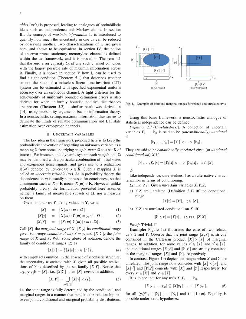
Fig. 1. Examples of joint and marginal ranges for related and unrelated uv’s.

Using this basic framework, a nonstochastic analogue ofstatistical independence can be defined:

Definition 2.1 (Unrelatedness): A collection of uncertainvariables Y1, . . . ,Ym is said to be (unconditionally) unrelatedif

JY1, . . . ,YmK = JY1K×·· ·× JYmK.

They are said to be conditionally unrelated given (or unrelatedconditional on) X if

JY1, . . . ,Ym|xK = JY1|xK×·· ·× JYm|xK, x ∈ JXK.

♦Like independence, unrelatedness has an alternative charac-

terization in terms of conditioning:Lemma 2.1: Given uncertain variables X ,Y,Z,a) Y,Z are unrelated (Definition 2.1) iff the conditional

rangeJY |zK = JY K, z ∈ JZK.

b) Y,Z are unrelated conditional on X iff

JY |z,xK = JY |xK, (z,x) ∈ JZ,XK.

Proof: Trivial. Example: Figure 1a) illustrates the case of two related

uv’s X and Y . Observe that the joint range JX ,Y K is strictlycontained in the Cartesian product JXK× JY K of marginalranges. In addition, for some values x′ ∈ JXK and y′ ∈ JY K,the conditional ranges JX |y′K and JY |x′K are strictly containedin the marginal ranges JXK and JY K, respectively.

In contrast, Figure 1b) depicts the ranges when X and Y areunrelated. The joint range now coincides with JXK× JY K, andJX |y′K and JY |x′K coincide with JXK and JY K respectively, forevery x′ ∈ JXK and y′ ∈ JY K.

It is to see that for any uv’s X ,Y1, . . . ,Ym,

JX |y1, . . . ,ymK⊆ JX |y1K∩·· ·∩ JX |ymK, (6)

for all (yi)mi=1 ∈ JY1K× ·· ·JYmK and i ∈ [1 : m]. Equality is

possible under extra hypotheses:

3

Lemma 2.2: Let X ,Y1, . . . ,Ym be uncertain variables s.t.Y1, . . . ,Ym are unrelated conditional on X (Definition 2.1). Then∀(y1, . . . ,ym) ∈ JY1, . . . ,YmK,

JX |y1, . . . ,ymK = JX |y1K∩·· ·∩ JX |ymK. (7)

Proof: See appendix A. The second item in Lemma 2.1 motivates the following

definition:Definition 2.2 (Markov Uncertainty Chains): The

uncertain variables X , Y and Z are said to form a Markovuncertainty chain X↔Y ↔ Z if X ,Z are unrelated conditionalon Y (Definition 2.1).♦Remarks: By the symmetry of Definition 2.1, Z↔ Y ↔ X

is also a Markov uncertainty chain.Before closing this section, it is noted that the framework

developed above is not equivalent to treating input variableswith known, bounded ranges as uniformly distributed rv’s.Such an approach is still probabilistic, and the output rv’s mayhave nonuniform distributions despite the uniform inputs. Incontrast, in the uv model here, only the ranges are considered,and no distributions are derived at any stage.

For instance, consider an additive bounded noise channelwith output Y = X +N, where the input X and noise N rangeon the interval [−0.5,0.5]. If X and N are taken to be mutuallyindependent, uniform rv’s, then Y has a triangular distributionon [−1,1], with small values of Y more probable than largeones. However, if X and N are treated as unrelated uv’s, thenall that can be inferred about Y is that it has range [−1,1],with all values in this range being equally possible.

Naturally, this lack of statistical structure does not suit allapplications. However, as discussed in section I, such structureis often excess to requirements, e.g. in problems with worst-case objectives and bounded variables as in section V. A uv-based approach is arguably more natural in these settings.

III. MAXIMIN INFORMATION

The framework introduced above is now used to define anonstochastic analogue I∗ of Shannon’s mutual informationfunctional. Two characterizations of I∗ are developed andshown to be equivalent (Definition 3.2 and Corollary 3.1).

Throughout this section, X ,Y are arbitrary uncertain vari-ables (uv’s) with marginal ranges JXK and JY K (1), jointrange JX ,Y K (3), and conditional range family JX |Y K (4). Setcardinality is denoted by | · |, with the value ∞ permitted, andall logarithms are to base 2.

A. Previous WorkIt is useful to first recall the nonprobabilistic formulations of

entropy and information mentioned in section I. Though orig-inally defined in different settings, for the sake of notationalcoherence they are discussed here using the uv framework ofsection II.

In loose terms, the entropy of a variable quantifies theprior uncertainty associated with it. For discrete-valued X , thisuncertainty may be captured by the (marginal) Hartley or 0-entropy

H0[X ] := log |JXK| ∈ [0,∞], (8)

If JXK has Lebesgue measure µ on Rn, then the (marginal)Renyi differential 0-entropy is defined as

h0[X ] := log µJXK ∈ [−∞,∞]. (9)

A related construction is the ε-entropy, which is the log-cardinality of the smallest partition of a given metric spacesuch that each partition set has diameter no greater than ε > 0[5]. None of these concepts require a probability space.

Two distinct notions of information have been proposedbased on the 0-entropies above. In [8], a worst-case approachis taken to first define the (conditional) 0-entropy of X givenY as

H0[X |Y ] := ess supy∈JYK

log |JX |yK| ∈ [0,∞]. (10)

If every set in the family JX |Y K is µ-measurable on Rn, thenthe (conditional) differential 0-entropy of X given Y is

h0[X |Y ] := ess supy∈JYK

log µJX |yK ∈ [−∞,∞]. (11)

Noting that Shannon information can be expressed as thedifference between the marginal and conditional entropies, anonstochastic 0-information functional I0 is then defined in [8]as

I0[X ;Y ] := H0[X ]−H0[X |Y ]≡ ess infy∈JYK

log(|JXK||JX |yK|

)(12)

if X is discrete-valued with H0[X |Y ]< ∞, and as

I0[X ;Y ] := h0[X ]−h0[X |Y ]≡ ess infy∈JYK

log(

µJXKµ (JX |yK)

)(13)

if X is continuous-valued with h0[X ;Y ] < ∞. In other words,the 0-information that can be gained about X from Y is theworst-case log-ratio of the prior to posterior uncertainty setsizes.1

The definition above is inherently asymmetric, i.e. I0[X ;Y ] 6=I0[Y ;X ]. A different and symmetric nonstochastic informationindex had been previously proposed in [9]. In that formulation,a conditional entropy was first defined as the differencebetween the joint and marginal Hartley entropies, in analogywith Shannon’s theory. The information transmission T[X ;Y ]was then defined as the difference between the marginal andconditional entropies, yielding the symmetric formula

T[X ;Y ] := H0[X ]+H0[Y ]−H0[X ,Y ].

Continuous variables with convex ranges admitted a similarconstruction, with H0 replaced not with h0 but a projection-based, isometry-invariant functional.

Though these concepts are intuitively appealing and sharesome desirable properties with Shannon information, theyhave two weaknesses. Firstly, they do not treat continuous-and discrete-valued uv’s in a unified way. In particular, it isunclear how to apply the approach of [9] to mixed pairs of

1Note that in 1965, Kolmogorov had defined log |JX |yK| as a ‘combinatorial’conditional entropy and the log-ratio log(|JXK|/|JX |yK|) as a measure ofinformation gain. However, these quantities have the defect of depending onthe observed value Y = y, and thus are associated with a specific posterioruncertainty set JX |yK. In contrast, (10)–(13) and (16) are functions of thefamily JX |YK of all possible posterior uncertainty sets.

4

variables, e.g. a digital symbol encoding a continuous state,or to continuous variables with nonconvex ranges.

Secondly and more importantly, their operational relevancefor problems involving communication has not been generallyestablished. While the worst-case log-ratio approach of [8] hasbeen used to find minimum bit rates for stabilization over anerrorless digital channel, it is not obvious how to apply it iftransmission errors occur.

For these reasons, an alternative approach is pursued in theremainder of this section.

B. I∗ via the Overlap Partition

The nonstochastic information index I∗ proposed in thissubsection quantifies the information that can be gained aboutX from Y in terms of certain structural properties of thefamily JX |Y K of posterior uncertainty sets. These propertiesare described below:

Definition 3.1 (Overlap Connectedness/Isolation):a) A pair of points x and x′ ∈ JXK is called JX |Y K-overlap

connected, denoted x ! x′, if ∃ a finite sequenceJX |yiKn

i=1 of conditional ranges such that x ∈ JX |y1K,x′ ∈ JX |ynK and each conditional range has nonempty in-tersection with its predecessor, i.e. JX |yiK∩JX |yi−1K 6= /0,for each i ∈ [2, . . . ,n].

b) A set A⊆ JXK is called JX |Y K-overlap connected if everypair of points in A is overlap connected.

c) A pair of sets A,B is called JX |Y K-overlap isolated ifno point in A is overlap connected with any point in B.

d) An JX |Y K-overlap isolated partition (of JXK) is a parti-tion of JXK where every pair of distinct member-sets isoverlap isolated.

e) An JX |Y K-overlap partition is an overlap-isolated parti-tion each member-set of which is overlap connected.

♦Remarks: For conciseness, the qualifier JX |Y K- will often

dropped when there is no risk of confusion about the condi-tional range family of interest. Note that any point or set isautomatically overlap connected with itself. In addition, x′ liesin the same overlap partition set as x iff x′! x.

Symmetry and transitivity guarantee that a unique overlappartition always exists:

Lemma 3.1 (Unique Overlap Partition): There is a uniqueJX |Y K-overlap partition of JXK (Definition 3.1), denotedJX |Y K∗. Every set C ∈ JX |Y K∗ is expressible as

C = x ∈ JXK : x! C=⋃

B∈JX |YK:B!CB. (14)

Furthermore, every JX |Y K-overlap isolated partition P ofJXK satisfies

|P| ≤ |JX |Y K∗|, (15)

with equality iff P = JX |Y K∗.Proof: See appendix B. Remarks: The self-referential identities in (14) are needed

to prove certain key results later. The first equality says thateach element C of the overlap partition coincides with the setof all points that are overlap connected with it. The second

4|X y2|X y

1|X y 5|X y3|X y1| y 5| y

1P 2P

1 2*| ,X Y = P P

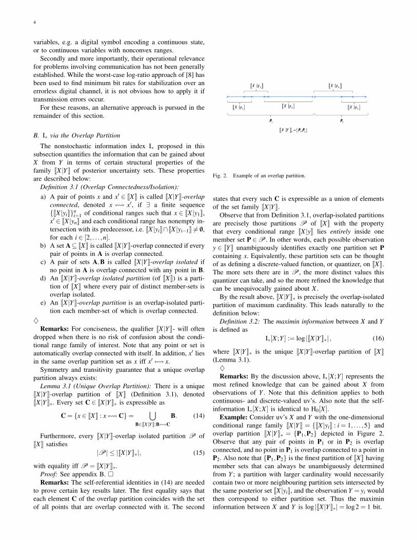
Fig. 2. Example of an overlap partition.

states that every such C is expressible as a union of elementsof the set family JX |Y K.

Observe that from Definition 3.1, overlap-isolated partitionsare precisely those partitions P of JXK with the propertythat every conditional range JX |yK lies entirely inside onemember set P ∈P . In other words, each possible observationy ∈ JY K unambiguously identifies exactly one partition set Pcontaining x. Equivalently, these partition sets can be thoughtof as defining a discrete-valued function, or quantizer, on JXK.The more sets there are in P , the more distinct values thisquantizer can take, and so the more refined the knowledge thatcan be unequivocally gained about X .

By the result above, JX |Y K∗ is precisely the overlap-isolatedpartition of maximum cardinality. This leads naturally to thedefinition below:

Definition 3.2: The maximin information between X and Yis defined as

I∗[X ;Y ] := log |JX |Y K∗| , (16)

where JX |Y K∗ is the unique JX |Y K-overlap partition of JXK(Lemma 3.1).♦Remarks: By the discussion above, I∗[X ;Y ] represents the

most refined knowledge that can be gained about X fromobservations of Y . Note that this definition applies to bothcontinuous- and discrete-valued uv’s. Also note that the self-information I∗[X ;X ] is identical to H0[X ].

Example: Consider uv’s X and Y with the one-dimensionalconditional range family JX |Y K = JX |yiK : i = 1, . . . ,5 andoverlap partition JX |Y K∗ = P1,P2 depicted in Figure 2.Observe that any pair of points in P1 or in P2 is overlapconnected, and no point in P1 is overlap connected to a point inP2. Also note that P1,P2 is the finest partition of JXK havingmember sets that can always be unambiguously determinedfrom Y ; a partition with larger cardinality would necessarilycontain two or more neighbouring partition sets intersected bythe same posterior set JX |yiK, and the observation Y = yi wouldthen correspond to either partition set. Thus the maximininformation between X and Y is log |JX |Y K∗|= log2 = 1 bit.

5

It is easy to verify that I∗ 6= I0.Example: Let X and Z be unrelated uv’s with JXK= 0,1

and JZK = 0,1, and define the uv Y by Y = X if Z = 0and Y = 2 if Z = 1. The family JY |XK consists of thesets JY |0K = 0,2 and JY |1K = 1,2. The overlap partitionJY |XK∗ has only one set, 0,1,2, so I∗[Y ;X ] = log1 = 0.However I0[Y ;X ] = log 3

2 , since the largest cardinality of setsin JY |XK is 2.

Finally, note that I∗[X ;Y ] was originally defined in [1] as

supF∈F JXK

minC∈JX |YK∗

log(|F||F∩C|

),

where F JXK is the family of all finite subsets of JXK; hence thename ‘maximin’ information. This log-ratio characterizationis close in spirit to (12)–(13) and can be shown to beequivalent to (16). However, since it does not have as simplean interpretation as (16) and is not needed for any of the resultshere, there will be no further discussion of it in what follows.

C. I∗ via the Taxicab Partition

The definition of maximin information above is based purelyon the conditional range family JX |Y K. As JY |XK will notgenerally be the same, it may seem that I∗ could be asym-metric in its arguments. However, it turns out that I∗ can bereformulated symmetrically in terms of the joint range JX ,Y K.A few additional concepts are needed in order to present thischaracterization.

Definition 3.3 (Taxicab Connectedness/Isolation):a) A pair of points (x,y) and (x′,y′) ∈ JX ,Y K is called

taxicab connected if there is a taxicab sequence con-necting them, i.e. a finite sequence (xi,yi)n

i=1 of pointsin JX ,Y K such that (x1,y1) = (x,y), (xn,yn) = (x′,y′)and each point differs in at most one coordinate fromits predecessor, i.e. yi = yi−1 and/or xi = xi−1, for eachi ∈ [2, . . . ,n].

b) A set A ⊆ JX ,Y K is called taxicab connected if everypair of points in A is taxicab connected in JX ,Y K.

c) A pair of sets A,B is called taxicab isolated if no pointin A is taxicab connected in JX ,Y K to any point in B.

d) A taxicab-isolated partition (of JX ,Y K) is a cover ofJX ,Y K such that every pair of distinct sets in the coveris taxicab isolated.

e) A taxicab partition (of JX ,Y K) is a taxicab-isolatedpartition of JX ,Y K each member-set of which is taxicabconnected.

♦Remarks: Note that any point or set is automatically

taxicab connected with itself. In addition, taxicab connected-ness/isolation in JX ,Y K is identical to that in JY,XK, with theorder of elements in each pair reversed. Consequently, anytaxicab-isolated partition of JX ,Y K is in one-to-one correspon-dence with one of JY,XK.

Taxicab-isolated partitions have the property that the par-ticular member set T that contains a given point (x,y) isuniquely determined by x and by y alone. The argument isby contradiction: if x is associated with two sets T,T′ in theoverlap-isolated partition, i.e. (x,y) ∈ T and (x,y′) ∈ T′ for

y

([X,Y] = shaded area)

y yy y y

x

a) Two points connected in taxicab

x x

b) Disconnected in taxicab & usual senses c) Ta icab disconnected a) Two points connected in taxicab,

but not usual, sense. & usual senses c) Taxicab disconnected,

but connected in usual sense

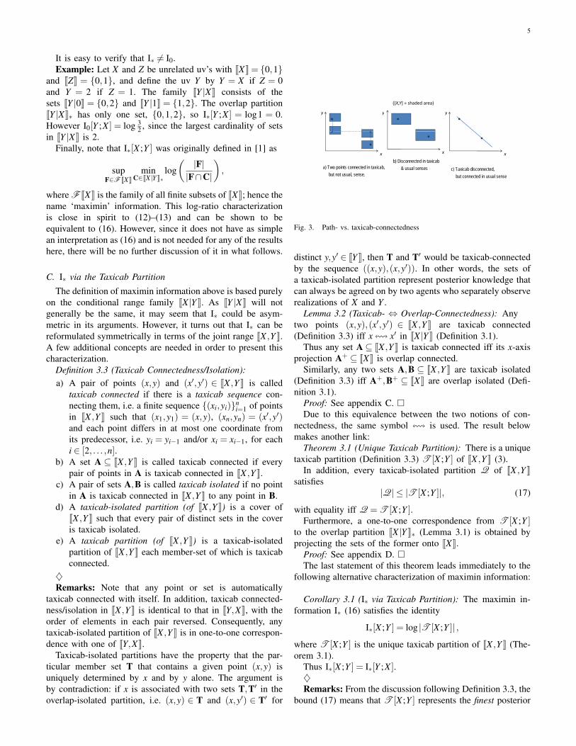
Fig. 3. Path- vs. taxicab-connectedness

distinct y,y′ ∈ JY K, then T and T′ would be taxicab-connectedby the sequence ((x,y),(x,y′)). In other words, the sets ofa taxicab-isolated partition represent posterior knowledge thatcan always be agreed on by two agents who separately observerealizations of X and Y .

Lemma 3.2 (Taxicab- ⇔ Overlap-Connectedness): Anytwo points (x,y),(x′,y′) ∈ JX ,Y K are taxicab connected(Definition 3.3) iff x! x′ in JX |Y K (Definition 3.1).

Thus any set A⊆ JX ,Y K is taxicab connected iff its x-axisprojection A+ ⊆ JXK is overlap connected.

Similarly, any two sets A,B ⊆ JX ,Y K are taxicab isolated(Definition 3.3) iff A+,B+ ⊆ JXK are overlap isolated (Defi-nition 3.1).

Proof: See appendix C. Due to this equivalence between the two notions of con-

nectedness, the same symbol ! is used. The result belowmakes another link:

Theorem 3.1 (Unique Taxicab Partition): There is a uniquetaxicab partition (Definition 3.3) T [X ;Y ] of JX ,Y K (3).

In addition, every taxicab-isolated partition Q of JX ,Y Ksatisfies

|Q| ≤ |T [X ;Y ]|, (17)

with equality iff Q = T [X ;Y ].Furthermore, a one-to-one correspondence from T [X ;Y ]

to the overlap partition JX |Y K∗ (Lemma 3.1) is obtained byprojecting the sets of the former onto JXK.

Proof: See appendix D. The last statement of this theorem leads immediately to the

following alternative characterization of maximin information:

Corollary 3.1 (I∗ via Taxicab Partition): The maximin in-formation I∗ (16) satisfies the identity

I∗[X ;Y ] = log |T [X ;Y ]| ,

where T [X ;Y ] is the unique taxicab partition of JX ,Y K (The-orem 3.1).

Thus I∗[X ;Y ] = I∗[Y ;X ].♦Remarks: From the discussion following Definition 3.3, the

bound (17) means that T [X ;Y ] represents the finest posterior

6

y

1Q

2T

2Q

1T

P P

x

1P 2P

1 2 1 2 1 2* *[ ; ] , , | , , | , .X Y X Y Y X= = =T T P P Q QT

Fig. 4. Taxicab and Overlap Partitions

knowledge that can be agreed on from individually observingX and Y . The log-cardinality of this partition has considerableintuitive appeal as an index of information. Indeed, if X andY are discrete rv’s, then the elements of the taxicab partitioncorrespond to the connected components of the bipartite graphthat describes (x,y) pairs with nonzero joint probability. In[13], the Shannon entropy of these connected components wascalled zero-error information and used to derive an intrinsicbut stochastic characterization of the zero-error capacity C0of discrete memoryless channels. Maximin information cor-responds rather to the Hartley entropy of these connectedcomponents. In section IV, it will be seen to yield an analogousnonstochastic characterization that is valid for discrete- orcontinuous-valued channels.

Example: The shaded regions in Figure 4 depict the jointrange JX ,Y K of uv’s X ,Y having the conditional range familyJX |Y K of Figure 2. The taxicab partition T [X ;Y ] consists ofthe sets T1 and T2; it can be seen that every pair of pointsin each set is taxicab connected, and no point in one set istaxicab-connected with a point in the other. Projecting T1 andT2 onto JXK yields P1 and P2, the sets comprising the overlappartition JX |Y K∗. Similarly, JY |XK∗ consists of the projectionsQ1 and Q2 of T1 and T2 onto JY K.

If two agents observe X and Y separately, then they willalways be able to agree on the index Z ∈ 1,2 of the uniquetaxicab partition set TZ that contains (X ,Y ), since it is alsothe index of the overlap partition sets PZ and QZ that containX and Y respectively. The amount of information they shareis then log |T [X ;Y ]|= log |JX |Y K∗|= log |JY |XK∗|= 1 bit.

D. Properties of Maximin Information

Two important properties of maximin information are nowestablished. These properties are also exhibited by Shannoninformation and will be needed to prove Theorem 5.1.

Lemma 3.3 (More Data Can’t Hurt): The maximin infor-mation I∗ (16) satisfies

I∗[X ;Y ]≤ I∗[X ;Y,Z]. (18)

Proof: By Definition 3.1, every set C ∈ JX |Y,ZK∗ is overlapconnected in JX |Y,ZK. As JX |y,zK ⊆ JX |yK, C is also overlapconnected in JX |Y K. Pick a set C′ ∈ JX |Y K∗ that intersectsC. As C′ is overlap connected in JX |Y K, it also ! C. ThusC ⊆ C′, since by (14) C′ must include all points ! C′.Consequently, there is only one C′ for each C.

Furthermore, since JX |Y,ZK∗ covers JXK, every set of JX |Y K∗must intersect and thus include some of its set(s). Thus the mapC 7→C′ is a surjection from JX |Y,ZK∗→ JX |Y K∗, implying that|JX |Y,ZK∗| ≥ |JX |Y K∗|.

Lemma 3.4 (Data Processing): If X ↔Y ↔ Z is a Markovuncertainty-chain (Definition 2.2), then the maximin informa-tion I∗ (16) satisfies

I∗[X ;Z]≤ I∗[X ;Y ]. (19)

Proof: By Lemma 3.3,

I∗[X ;Z]≤ I∗[X ;Y,Z](16)= log |JX |Y,ZK|∗.

By Definition 2.2, JX |y,zK = JX |yK for every ∀y ∈ JY K andz ∈ JZ|yK, so JX |Y,ZK∗ = JX |Y K∗. Substituting this into theRHS of the equation above and applying (16) again completesthe proof.

Remark: By the symmetry of Markov uncertainty chainsand maximin information, I∗[X ;Z]≤ I∗[Y ;Z].

E. Discussion

Maximin information is a more conservative index thanShannon information I. For instance, Corollary 3.1 impliesthat unrelated uv’s must share 0 maximin information, butthe converse does not hold, unlike the analogous case withShannon information. This is because I∗[X ;Y ] is the largestcardinality of JX ,Y K-partitions such that the unique partitionset containing any realization (x,y) can be determined byobserving either x or y alone. Even if X and Y are related,there may be no way to split the joint range into two or moresets that are each unambiguously identifiable in this way.

Example: Let JX ,Y K = (0,0),(0,1),(1,1). As JX ,Y K 6=JXK×JY K = 0,12, X and Y are related. However, every pairof points in JX ,Y K is taxicab-connected, so T [X ;Y ] has onlyone set, JX ,Y K, and I∗[X ;Y ] Cor. 3.1

= 0. See also Figure 5 forother examples.

This conservatism might suggest that I∗ could be derivedfrom Shannon information via a variational principle, i.e. as

infI[X ;Y ] : X ,Y rv’s with given support JX ,Y K .

However, such an approach would be too conservative, sincethe infimum can be zero even when the maximin informationis strictly positive. A formal proof of this is not given due tospace constraints, but a sketch of the argument follows. Let qbe a (suitably well-behaved) joint probability density function(pdf) that is strictly positive on the Lebesgue measurablesupport JX ,Y K of Figure 3(b) and that has finite Shannoninformation. Pick a point x′,y′ in the interior of the supportand for any ε and sufficiently small r > 0, let X ,Y be rv’s withjoint pdf pX ,Y = (1− ε)ux′,y′,r + εq, where ux′,y′,r is a uniformpdf ux′,y′ on a square of dimension r > 0 centred at (x′,y′).Observe that if (r,ε) = (0,0), the joint pdf becomes a unit

7

y([X,Y] = shaded area)

yy y

x

, related, b t I [ ] 0X Y

X Y

x

, related, X Yx

, unrelated, X Y*but I [ ; ] 0X Y =

* 2I [ ; ] log 2 1X Y = = *I [ ; ] 0X Y =

Fig. 5. Zero I∗ does not imply unrelatedness

delta function centred at (x′,y′), which automatically yieldszero mutual information. As I[X ;Y ] must vary continuouslywith ε,r ≥ 0, it follows that I[X ;Y ]→ 0 as (ε,r)→ (0,0).The nonnegativity of Shannon information then implies thatthe infimum above must be zero, but the maximin informationremains 1.

IV. CHANNELS AND CAPACITY

In this section, a connection is made between maximin in-formation and the problem of transmission over an erroneous,discrete-time channel.

A. Stationary Memoryless Uncertain ChannelsLet X∞ be the space of all X-valued, discrete-time functions

x : Z≥0 → X. An uncertain (discrete-time) signal X is amapping from the sample space Ω to some function spaceX ⊆ X∞ of interest. Confining this mapping to any timet ∈ Z≥0 yields an uncertain variable (uv), denoted X(t). Thesignal segment (X(t))b

t=a is denoted X(a : b). As with uv’s,the dependence on ω ∈ Ω will not usually be indicated: thusthe statements X ∈ A and X(t) = x(t) mean that X(ω) ∈ Aand X(ω)(t) = x(t) respectively. Also note that JXK here is asubset of the function space X .

A nonstochastic parallel of the standard notion of a station-ary memoryless channel in communications can be defined asfollows:

Definition 4.1: Given an input function space X ⊆ X∞

and a set-valued transition function T : X→ 2Y, a stationarymemoryless uncertain channel maps any uncertain input signalX with range JXK⊆X to an uncertain output signal Y so that

JY (0 : t)|x(0 : t)K = T(x(0))×·· ·×T(x(t)),x(0 : t) ∈ JX(0 : t)K, t ∈ Z≥0.(20)

The set-valued reverse transition function R : Y→ 2X of thechannel is

R(y) := x ∈ X : T(x) 3 y, y ∈ Y. (21)

Remarks: The set-valued map T here plays the role of atime-invariant transition probability matrix or kernel in com-munications theory. The input function class X is included

to handle possible constraints such as limited time-averagedtransmission power or input run-lengths, though in the rest ofthis paper X is taken as X∞.

The definition above implicitly assumes no feedback fromthe receiver back to the transmitter. If such feedback is presentthen by arguments similar to Massey’s [15], a more generaldefinition must be used - see [16].

The following lemma shows that the conditional range ofthe input sequence given an output sequence is defined by thereverse transition function and the unconditional input range.

Lemma 4.1: Given a stationary memoryless uncertain chan-nel (Definition 4.1) with reverse transition function R (21),

JX(0 : t)|y(0 : t)K = JX(0 : t)K∩t

∏i=0

R(y(i))︸ ︷︷ ︸=:R(y(0:t))

, y(0 : t) ∈ Yt+1

(22)and for any valid pair X ,Y of uncertain input and outputsignals.

Proof: See appendix E. The largest information rate across a channel is formally

defined as follows:Definition 4.2: The peak maximin information rate of a

stationary memoryless uncertain channel (Definition 4.1) is

R∗ := supt∈Z≥0,X :JXK⊆X

I∗[X(0 : t);Y (0 : t)]t +1

, (23)

where X is the input function space and Y is the uncertainoutput signal yielded by the uncertain input signal X .♦It can be shown that the term under the supremum over

time on the RHS is super-additive. A standard result calledFekete’s lemma then states that the supremum over time onthe RHS of (23) is achieved in the limit as t→ ∞. This leadsimmediately to the following identity:

Lemma 4.2: For any stationary memoryless uncertain chan-nel (Definition 4.1), the peak maximin information rate R∗ (23)satisfies

R∗ = limt→∞

supX :JXK⊆X

I∗[X(0 : t);Y (0 : t)]t +1

, (24)

where X is the input function space and Y is the uncertainoutput signal yielded by X .

∇

B. Zero-Error Capacity

It is next shown how R∗ relates to the concept of zero-error capacity C0 [11], [12], which Shannon introduced afterits more famous sibling the (ordinary) capacity C [10]. Asdescribed in section I, the zero-error capacity of a stochasticchannel is defined as the largest average block-coding bit-rateat which input “messages” can be transmitted while ensuringthat the probability of a decoding error is exactly zero (notjust arbitrarily small, as with the usual capacity). It is wellknown that C0 does not depend on the probabilistic natureof the channel, in the sense that the specific values of thenonzero transition probabilities play no role. This suggests that

8

C0 ought to be defineable using the nonstochastic frameworkof this paper.

To see this, observe that a length-(t + 1) zero-error blockcode may be represented as a finite set F ⊆ Xt+1, whereeach codeword f ∈ A corresponds to a distinct “message”.The average coding rate is thus (log |F|)/(t + 1) bits/sample,under the constraint that any received output sequence y(0 : t)corresponds to at most one possible f . In other words t ∈Z≥0,a set F ⊆ Xt+1 of codewords is valid iff for each possiblechannel output sequence y(0 : t) ∈ Yt+1, |F∩R(y(0 : t))| ≤ 1.Thus the zero-error capacity may be defined operationally as

C0 := supt∈Z≥0,F∈F (Xt+1)

log |F|t +1

= limt→∞

supF∈F (Xt+1)

log |F|t +1

, (25)

where the limit again follows from superadditivity and

F (Xt+1) :=F ∈F (Xt+1) : ∀y(0 : t) ∈ Yt+1, |F∩R(y(0 : t))| ≤ 1

,(26)

with F (Xt+1) the family of all finite subsets of Xt+1 and R,the reverse block transition function (22).

The main result of this section shows that C0 admits anintrinsic characterization in terms of maximin informationtheory:

Theorem 4.1 (C0 via Maximin Information): For any sta-tionary memoryless uncertain channel with input functionspace X =X∞ (Definition 4.1), the peak maximin informationrate R∗ (Definition 4.2) equals the zero-error capacity C0 (25).

Proof: As JX(0 : t)|Y (0 : t)K∗ is a partition of JX(0 : t)K,

|JX(0 : t)|Y (0 : t)K∗|= sup

F∈F JX(0:t)K:∀C∈JX(0:t)|Y (0:t),|F∩C|≤1K∗|F|

(14)≤ sup

F∈F JX(0:t)K:∀B∈JX(0:t)|Y (0:t),|F∩B|≤1K|F|

(22)= sup

F∈F JX(0:t)K:∀y(0:t)∈Yt+1,|F∩R(y(0:t))|≤1|F|

(26)≤ sup

F∈F (Xt+1)

|F|(25)≤ 2C0(t+1). (27)

⇒ R∗(16),(23)≤ C0. (28)

It is next shown that ∀t ∈ Z≥0, ∃ a uv X(0 : t) for which(27) is an equality. For any F ∈ F (Xt+1) (26), let X(0 : t) bea surjection from Ω→ F.2 Then no point in JX(0 : t)K = Fis overlap connected (Definition 3.1) with any other, since atleast one of the conditional ranges JX(0 : t)|y(0 : t)K overlap-connecting them would then have 2 or more distinct points;this is impossible by (22) and (26). Thus the overlap partitionJX(0 : t)|Y (0 : t)K∗ (Lemma 3.1) of JX(0 : t)K is a family of|JX(0 : t)K| = |F| singletons, comprising the individual pointsof JX(0 : t)K = F.

If F (Xt+1) has a set F∗ of maximum cardinality, thenchoosing F = F∗ forces the LHS of (27) to coincide with the

2As in the mutual-information characterization of Shannon capacity, it isimplicit that the underlying sample space Ω is infinite, so that such a surjectionalways exists for each t ∈ Z≥0.

RHS. Otherwise, the RHS of (27) will be infinite and F maybe chosen to have arbitrarily large cardinality, again yieldingequality in (27), by (16). This achieves equality in (28).

Remarks: This result shows that the largest average bit-ratethat can be transmitted across a stationary memoryless uncer-tain channel with errorless decoding coincides with the largestaverage maximin information rate across it. This parallelsShannon’s channel coding theorem for stochastic memorylesschannels and arguably makes I∗ more relevant for problemsinvolving communication than other nonstochastic informationindices.

It must be noted that ensuring exactly zero decoding er-rors is a stringent requirement and is impossible over manycommon channels, such as the the binary symmetric, binaryerasure and additive white Gaussian noise channels, whichhave C0 = 0. However, a number of channels are known topossess nonzero C0, such as the pentagon and additive boundednoise channels. Zero-error capacity is also an object of studyin graph theory, where it is related to the clique number. See[12] for a comprehensive survey of the literature on C0.

V. STATE ESTIMATION OF LINEAR SYSTEMS OVERERRONEOUS CHANNELS

In this section, maximin information is used to study theproblem of estimating the states of a linear time-invariant(LTI) plant via a stationary memoryless uncertain channel(Definition 4.1), without channel feedback. First, some relatedprior work is discussed.

A. Prior Work

In the case where the channel is an errorless digital bit-pipe,the state estimation problem is formally equivalent to feedbackstabilization with control inputs known to both encoder anddecoder. The central result in this scenario is the so-called“data rate theorem”, which states that the estimation error orplant state can be stabilized or taken to zero iff the sum H ofthe log-magnitudes of the unstable eigenvalues of the systemis less than the channel bit-rate. This condition holds in bothdeterministic and probabilistic settings, and under differentnotions of convergence or stability, e.g. uniform, rth momentor almost surely (a.s.) [17], [18], [19], [20], [21], [22], [23].See also [24] for recent work on quantized estimation ofstochastic LTI systems.

However, if transmission errors occur, then the stabilizabil-ity and estimation conditions become highly dependent on thesetting and objective, leading to a variety of different criteria.For instance, given a stochastic discrete memoryless channel(DMC) and a noiseless LTI system with random initial state,a.s. convergence of the state or estimation error to zero ispossible if and (almost) only if the ordinary channel capacityC ≥ H; this was proved for digital packet-drop channels withacknowledgements in [25], and for general DMC’s with orwithout channel feedback in [26]. The same result also holdsfor asymptotic stabilizability via an additive white Gaussiannoise channel [27], with no channel feedback. See also [28]for bounds on mean-square-error convergence rates for stateestimation over stochastic DMC’s, without channel feedback.

9

Suppose next that additive stochastic noise perturbs the plantand the objective is to bound the rth moment of the states orestimation errors. Assuming channel feedback, bounded noiseand scalar states, the achievability of this goal is determinedby the anytime capacity of the channel [29]. Other relatedarticles are [30], [31], [32] - the first two consider momentstabilization over errorless channels with randomly varyingbit-rates known to both transmitter and receiver, and the laststudies mean-square stabilization via DMC’s with no channelfeedback. See also the recent papers [33], [34] for explicitconstructions of error-correcting codes for control.

For the purposes of this section, the most relevant priorwork is [14] (see also [35]), in which the channel is modelledas a stochastic DMC, and the plant is LTI with randominitial state but is perturbed by additive nonstochastic boundeddisturbances. It was shown that if channel feedback is absent,then a.s. uniformly bounded estimation errors are possible iffH <C0, the zero-error capacity [11] of the channel. However,under perfect channel feedback the necessary and sufficientcondition becomes H <C0f, the zero-error feedback capacitydefined in [11]; the same criterion applies if the goal isto stabilize the plant states in the a.s. uniformly boundedsense, with or without channel feedback. As C0 and C0fare (often strictly) less than C, both these conditions aremore restrictive than for plants with stochastic or no processnoise, even if the disturbance bound is arbitrarily small. Inrough terms, the reason for the increased strictness is thatnonstochastic disturbances do not enjoy a law of large numbersthat averages them out in the long run. As a result it becomescrucial for no decoding errors to occur in the channel, notjust for their average probability to be arbitrarily small. Thisimportant result was proved using probability theory, a lawof large numbers and volume-partitioning arguments, but noinformation theory.

The scenarios considered in this section are similar to [14],with the chief difference being that that neither the initialstate nor the erroneous channel are modelled stochasticallyhere. As a consequence, probability and the law of largenumbers cannot be employed in the analysis. Instead, maximininformation is applied to yield necessary conditions that arethen be shown to be tight (Thms. 5.1 and 5.2). Only stateestimation without channel feedback is considered here, sincethe maximin-information theoretic analysis of systems withfeedback is significantly different - see [16] for some prelim-inary results.

In what follows, ‖.‖ denotes either the maximum norm ona finite-dimensional real vector space or the matrix norm itinduces, and Bl(x) denotes the corresponding l-ball y : ‖y−x‖ ≤ l centered at x.

B. Disturbance-Free LTI Systems

Consider an undisturbed linear time-invariant (LTI) system

X(t +1) = AX(t) ∈ Rn, (29)Y (t) = GX(t) ∈ Rp, t ∈ Z≥0, (30)

where the initial state X(0) is an uncertain variable (uv). Theoutput signal Y is causally encoded via an operator γ as

S(t) = γ (t,Y (0 : t)) ∈ S, t ∈ Z≥0. (31)

Each symbol S(t) is then transmitted over a stationary mem-oryless uncertain channel with set-valued transition functionS 7→ 2Q and input function space S∞ (Definition 4.1), yieldinga received symbol Q(t) ∈ Q. Note that the encoder is toldnothing about the values of these received symbols, i.e. thereis no channel feedback. These symbols are used to producea causal prediction X(t +1) of X(t +1) by means of anotheroperator η as

X(t +1)≡ η(t,Q(0 : t)) ∈ Rn, t ∈ Z≥0, X0 = 0. (32)

Let E(t) := X(t)− X(t) denote the prediction error.The pair (γ,η) is called a coder-estimator. Such a pair is

said to yield ρ-exponential uniformly bounded errors if forany uv X(0) with range ⊆ Bl(0),

supt∈Z≥0,ω∈Ω

ρ−t‖E(t)‖ ≡ sup

t∈Z≥0

supq

ρ−t‖E(t)‖

y< ∞, (33)

where l,ρ > 0 are specified parameters. If the stronger prop-erty

limt→∞

supω∈Ω

ρ−t‖E(t)‖ ≡ lim

t→∞sup

qρ−t‖E(t)‖

y= 0 (34)

holds, then ρ-exponential uniform convergence is said to beachieved.

Impose the following assumptions:DF1: The pair (G,A) in (29)–(30) is observable.DF2: For every t ∈ Z≥0, the channel output sequence

Q(0 : t) (Definition 4.1) is conditionally unrelated(Definition 2.1) with initial state X(0), given thechannel input sequence S(0 : t); i.e. X(0) ↔ S(0 :t)↔ Q(0 : t).

DF3: The convergence parameter ρ of (33)–(34) is strictlysmaller than the spectral radius of A.

Remarks: Condition DF1 can be relaxed to requiring theobservability of A on the invariant subspace correspondingto eigenvalues greater than or equal to ρ in magnitude.Assumption DF2 basically states that the channel outputscan depend on the initial state only via the channel inputs.Condition DF3 entails negligible loss of generality, since if ρ

were to exceed the largest plant eigenvalue magnitude |λmax|,then the trivial estimator X(t) = 0 would achieve (34) andcommunication would not be needed.3

The main result of this subsection is given below:Theorem 5.1: Consider the linear time-invariant system

(29)–(30), with plant matrix A ∈ Rn×n, uncertain initial stateX(0) and outputs that are coded and estimated (31)–(32)without channel feedback, via a stationary memoryless uncer-tain channel (Definition 4.1) with zero-error capacity C0 ≥ 0(25). Let λ1, . . . ,λn be the eigenvalues of A and suppose thatAssumptions DF1–DF3 hold.

3The case ρ = |λmax| introduces technicalities that can be handled bymodifying to the arguments below; for the sake of conciseness it is notexplicitly treated here.

10

If there exists a coder-estimator that yields ρ-exponentialuniformly bounded estimation errors (33) with respect to anonempty l-ball Bl(0)⊂ Rn of initial states, then

C0 ≥ ∑i∈[1:n]:|λi|≥ρ

log∣∣∣∣λi

ρ

∣∣∣∣=: Hρ . (35)

Conversely, if the inequality in (35) holds strictly, then acoder-estimator without channel feedback can be constructedto yield ρ-exponential uniform convergence (34) on any initial-state l-ball.

1) Proof of Necessity: The necessity of (35) is establishedfirst. Without loss of generality, let the state coordinates bechosen so that A is in real Jordan canonical form (see e.g.[36], Theorem 3.4.5), i.e. it consists of m square blocks onits diagonal, with the jth block A j ∈ Rn j×n j having eitheridentical real eigenvalues or identical complex eigenvalues andconjugates for each j ∈ [1 : m]. Let the blocks be orderedby descending eigenvalue magnitude. For any j ∈ [1 : m],let X j(t) ∈ Rn j comprise those components of X(t) governedby the jth real Jordan block A j, and let E j(t), X j(t) ∈ Rn j

consist of the corresponding components of E(t) and X(t),respectively.

Let d ∈ [0 : n] denote the number of eigenvalues withmagnitude > ρ , including repeats. Pick arbitrary τ ∈ N and

ε ∈(

0,1− maxi:|λi|>ρ

ρ

|λi|

), (36)

and then divide the interval [−l, l] on the ith axis into

ki :=⌊∣∣∣∣ (1− ε)λi

ρ

∣∣∣∣τ⌋ (37)

equal subintervals of length 2l/ki, for each i ∈ [1 : d]. De-note the midpoints of the subintervals so formed by pi(s),s = 1, . . . ,ki, and inside each subinterval construct an intervalIi(s) centred at pi(s) but of shorter length l/ki. Define ahypercuboid family

H :=

(d

∏i=1

Ii(si)

)× [−l, l]n−d : si ∈ [1 : ki], i ∈ [1 : d]

(38)

and observe that any two hypercuboids ∈H are separated bya distance of l/ki along the ith axis for each i ∈ [1 : d]. Set theinitial state range JX(0)K =

⋃H∈H ⊂ Bl(0).

As JE j(t)K⊇ JE j(t)|q(0 : t−1)K,

diamJE j(t)K≥ diamJE j(t)|q(0 : t−1)K= diam

qAt

jX j(0)−η j (t,q(0 : t−1)) |q(0 : t−1)y

= diamq

AtjX j(0)|q(0 : t−1)

y(39)

≡ supu,v∈JX j(0)|q(0:t−1)K

‖Atj(u− v)‖

≥ supu,v∈JX j(0)|q(0:t−1)K

‖Atj(u− v)‖2√

n

≥ supu,v∈JX j(0)|q(0:t−1)K

σmin(Atj)‖u− v‖2√

n(40)

≥ supu,v∈JX j(0)|q(0:t−1)K

σmin(Atj)‖u− v‖√

n

≡ σmin(Atj)

diamJX j(0)|q(0 : t−1)K√n

,

t ∈ Z≥0, q(0 : t−1) ∈ JQ(0 : t−1)K, (41)

where diam(·) denotes set diameter under the maximum norm;(39) holds since translating a set in a normed space does notchange its diameter; ‖·‖2 denotes Euclidean norm; and σmin(·)denotes smallest singular value.

Now, an asymptotic identity of Yamamoto states that

limt→∞

(σmin(At

j))1/t

= |λmin(A j)|, where λmin(·) denotessmallest-magnitude eigenvalue (see e.g. [37], Thm 3.3.21). Asthere are only finitely many blocks A j, ∃tε ∈ Z≥0 s.t.

σmin(Atj)≥

(1− ε

2

)t|λmin(A j)|t , j ∈ [1 : m], t ≥ tε . (42)

In addition, for any region K in a normed vector space,

diam(K) ≡ supu,v∈K

‖u− v‖ ≤ supu,v∈K

‖u‖+‖v‖

= 2 supu∈K‖u‖. (43)

By (33), there then exists φ > 0 such that

φρt ≥ supJ‖E(t)‖K

≥ supJ‖E j(t)‖K(43)≥ 0.5diamJE j(t)K

(42),(41)≥

∣∣∣(1− ε

2

)λmin(A j)

∣∣∣t diamJX j(0)|q(0 : t−1)K2√

n,

j ∈ [1 : m], t ≥ tε . (44)

For some τ ∈ N, the hypercuboid family H (38) is anJX(0)|Q(0 : τ−1)K-overlap isolated partition (Definition 3.1)of JX(0)K. To see this, suppose in contradiction that ∃H ∈Hthat is overlap connected in JX(0)|Q(0 : τ−1)K with anotherhypercuboid in H . Then there would exist a set JX(0) :q(0 : τ−1)K containing a point u ∈ H and a point v in someH′ ∈H \H. Thus u j,v j ∈ JX j(0)|q(0 : τ−1)K, implying

‖u j− v j‖ ≤ diamJX j(0)|q(0 : τ−1)K(44)≤ 2

√nφρτ∣∣(1− ε/2)λmin(A j)

∣∣τ ,j ∈ [1 : m], τ ≥ tε . (45)

However, by construction any two hypercuboids ∈ H aredisjoint and separated by a distance of at least l/ki along theith axis for each i ∈ [1 : d]. Thus if A j is the real Jordan blockcorresponding to some eigenvalue λi, i ∈ [1 : d], then

‖u j− v j‖ ≥lki

(37)=

l⌊((1− ε)|λi|/ρ)τ

⌋≥ l

((1− ε)|λi|/ρ)τ =lρτ∣∣(1− ε)λmin(A j)

∣∣τ ,since all the eigenvalues of A j have equal magnitudes. TheRHS of this would exceed the RHS of (45) when τ ≥max(tε , t ′) is sufficiently large that

(1−ε/21−ε

)τ

> 2√

nφ/l, yield-ing a contradiction.

11

As H is an JX(0)|Q(0 : τ − 1)K-overlap isolated partitionof JX(0)K for sufficiently large τ ,

2I∗[X(0);Q(0:τ−1)] (16)= |JX(0)|Q(0 : τ−1)K∗|

(15)≥ |H |

=d

∏i=1

ki(37)=

d

∏i=1

⌊∣∣∣∣ (1− ε)λi

ρ

∣∣∣∣τ⌋≥

d

∏i=1

0.5∣∣∣∣ (1− ε)λi

ρ

∣∣∣∣τ (46)

=(1− ε)dτ

∣∣∏di=1 λi

∣∣τ2dρdτ

, (47)

where (46) follows from (36) and the inequality bxc> x/2, forevery x≥ 1. However, since X(0)↔ S(0 : τ−1)↔Q(0 : τ−1)is a Markov uncertainty-chain (Definition 2.2),

I∗[X(0);Q(0 : τ−1)]Lem. 3.4≤ I∗[S(0 : τ−1);Q(0 : τ−1)]

Def. 4.2≤ τR∗

Thm.4.1= τC0.

Substituting this into the LHS of (47), taking logarithms,dividing by τ and then letting τ → ∞ yields

C0 ≥ d log(1− ε)+d

∑i=1

log∣∣∣∣λi

ρ

∣∣∣∣ .As ε may be arbitrarily small, this establishes the necessity of(35).

2) Proof of Sufficiency: The sufficiency of (35) is straight-forward to establish. Define new state and measurement vec-tors X ′(t)= ρ−tX(t) and Y ′(t)= ρ−tY (t), for every t ∈Z≥0. Inthese new coordinates, the system equations (29)–(30) become

X ′(t +1) = (A/ρ)X ′(t) ∈ Rn, (48)Y ′(t) = GX ′(t) ∈ Rp, t ∈ Z≥0. (49)

By (35) and (25), ∀δ ∈ (0,C0−Hρ) ∃tδ > 0 s.t. ∀τ ≥ tδ , ∃ afinite set F⊆ Sτ with maxqτ−1

0 ∈Qτ |F∩R(qτ−10 )|= 1 and

Hρ <C0−δ ≤ (log |F|)/τ. (50)

Down-sample (48)–(49) by τ to obtain the LTI system

X ′ ((k+1)τ) = (A/ρ)τ X ′(kτ) ∈ Rn, (51)Y ′(kτ) = GX ′(kτ) ∈ Rp, k ∈ Z≥0. (52)

Now, |F| distinct codewords can be transmitted over thechannel and decoded without error once every τ samples.

Furthermore log |F|(50)> τHρ = sum of the unstable eigenvalue

log-magnitudes of (A/ρ)τ . By the “data rate theorem” (seee.g. [17]), there then exists a coder-estimator for the LTI down-sampled system (51)–(52) that estimates the states of (51) witherrors ‖X ′(kτ)−X ′k‖ tending uniformly to 0. For every t ∈Z≥0,write t = kτ+r for some k ∈Z≥0 and r ∈ [0 : τ−1], and definean estimator

X(t) := ρkτ+rArX ′k.

Then

ρ−t sup

ω∈Ω

‖X(t)− X(t)‖

= ρ−(kτ+r) sup

ω∈Ω

∥∥∥ρkτ ArX ′(kτ)−ρ

kτ ArX ′k∥∥∥

≤ ρ−r‖Ar‖ sup

ω∈Ω

∥∥X ′(kτ)− X ′k∥∥

≤ maxr∈[1:τ−1]

ρ−r‖Ar‖

supω∈Ω

∥∥X ′(kτ)− X ′k∥∥→ 0

as t, and hence k ≡ bt/τc, tend to ∞.

C. LTI Systems with Disturbances

The results and techniques of the previous subsection can bereadily adapted to analyze systems with disturbances. Supposethat, instead of (29)–(30), the plant state and output equationsare

X(t +1) = AX(t)+V (t) ∈ Rn, (53)Y (t) = GX(t)+W (t) ∈ Rp, t ∈ Z≥0, (54)

where the uncertain signals V and W represent additive processand measurement noise. The objective is uniform boundedness,i.e. (33) with ρ = 1. Make the following assumptions:

D1: The plant dynamics (53) are strictly unstable, i.e. thematrix A has spectral radius strictly larger than 1.

D2: The uncertain noise signals V and W are uniformlybounded, i.e. ∃c > 0 s.t. all possible signal realiza-tions v∈ JV K and w∈ JW K have `∞-norms ‖v‖,‖w‖≤c.

D3: The zero sequence is a possible process and mea-surement noise realization, i.e. 0 ∈ JV K∩ JW K.

D4: The initial state X(0), V and W are mutually unre-lated (Definition 2.1).

D5: For every t ∈ Z≥0, the channel output sequenceQ(0 : t) (Definition 4.1) is conditionally unrelated(Definition 2.1) with (X(0),V (0 : t−1),W (0 : t)),given the channel input sequence S(0 : t), i.e.(X(0),V (0 : t−1),W (0 : t))↔ S(0 : t)↔ Q(0 : t).

The following result holds:Theorem 5.2: Consider a linear time-invariant plant (53)–

(54), with plant matrix A ∈ Rn×n, uncertain initial state X(0),and bounded uncertain signals V and W additively corruptingthe dynamics and outputs respectively. Suppose the plantoutputs are coded and estimated (31)–(32) without feedbackvia a stationary memoryless uncertain channel (Definition 4.1)having zero-error capacity C0 ≥ 0 (25), and assume conditionsDF1 and D1–D5.

If there exists a coder-estimator (31)–(32) yielding uni-formly bounded estimation errors with respect to a nonemptyl-ball Bl(0)⊂ Rn of initial states, then

C0 ≥ ∑i∈[1:n]:|λi|≥1

log |λi|=: H, (55)

where λ1, . . . ,λn are the eigenvalues of A.Conversely, if (55) holds as a strict inequality, then a coder-

estimator can be constructed to yield uniform boundedness forany given l-ball of initial states.

12

Proof: Necessity is straightforward. If a coder-estimatorachieves uniform boundedness, then this uniform bound is notexceeded if the uncertain disturbances are realized as the zerosignal, which by hypothesis is an element of both JV K and JW K.By unrelatedness JX(0)|V = 0,W = 0K= JX(0)K, so the initialstate range is unchanged. Furthermore, condition D5 impliesX(0)↔ S(0 : t)↔ Q(0 : t), i.e. condition DF2. As uniformboundedness is just ρ-exponential uniform boundedness withρ = 1 (33), Theorem 5.1 applies immediately to yield (55).

The sufficiency of (55) is established next. By (55) and (25),∀δ ∈ (0,C0−H) ∃tδ > 0 s.t. ∀τ ≥ tδ , ∃ a finite set F⊆ Sτ withmaxqτ−1

0 ∈Qτ |F∩R(qτ−10 )|= 1 and

H <C0−δ ≤ (log |F|)/τ. (56)

Down-sample (53)–(54) by τ to obtain the LTI system

X ((k+1)τ) = Aτ X ′(kτ)+V ′τ(k) ∈ Rn, (57)Y (kτ) = GX(kτ)+W (kτ) ∈ Rp, k ∈ Z≥0,(58)

where the accumulated noise term V ′r (k) :=∑ri=0 Aτ−1−iV (kτ+

i) can be shown to be uniformly bounded over k ∈ Z≥0for each r ∈ [0 : τ − 1]. Now, |F| distinct codewords canbe transmitted over the channel and decoded without error

once every τ samples. Furthermore log |F|(56)> τH = sum of

the unstable eigenvalue log-magnitudes of Aτ . By the “datarate theorem” for LTI systems with bounded disturbancescontrolled or estimated over errorless channels, (see e.g. [17],[21], [19]), there then exists a coder-estimator for the LTIdown-sampled system (53)–(54) that estimates its states witherrors X(kτ)− Xk uniformly bounded over k ∈ Z≥0.

For every t ∈ Z≥0, write t = kτ + r for some k ∈ Z≥0 andr ∈ [0 : τ−1], and define an estimator

X(t) := ArXk.

Then

supω∈Ω

‖X(t)− X(t)‖

= supω∈Ω

∥∥ArX(kτ)+V ′r (k)−ArXk∥∥

≤ ‖Ar‖ supω∈Ω

∥∥X(kτ)− Xk∥∥+‖V ′r (k)‖

≤ maxr∈[1:τ−1]

‖Ar‖ supω∈Ω

∥∥X(kτ)− Xk∥∥+ max

r∈[1:τ−1]‖V ′r (k)‖.

As the RHS is uniformly bounded over k ∈ Z≥0, the proof iscomplete.

D. Discussion

Like the results of Matveev and Savkin [14] on LTI stateestimation via an erroneous channel without feedback, Thms.5.1 and 5.2 involve the zero-error capacity of the channel.In their formulation, the process and measurement noise aretreated as bounded unknown deterministic signals, but thechannel and initial state are modelled probabilistically. Theestimation objective is to achieve estimation errors that, withprobability (w.p.) 1, are uniformly bounded over all admissibledisturbances, and the necessity part of their result was provedwith the aid of a law of large numbers.

The main aims of this section have been to demonstratefirstly, that statistical assumptions are not necessary to capturethe essence of this problem (modulo zero-probability events);and secondly, that even with no probabilistic structure toexploit, information-theoretic techniques can be successfullyapplied, based on I∗. Although the channel and initial statehere are modelled nonstochastically and, furthermore, theestimation errors are to be bounded uniformly over all samplesω ∈ Ω, not just w.p.1, the achievability criterion (55) ofsubsection V-C essentially recovers the earlier result.4

In addition, unlike [14] and Theorem 5.2, Theorem 5.1assumes no disturbances and concerns performance as mea-sured by a specific convergence rate, not just bounded errors.The criterion (35) agrees with [14] when ρ = 1, but is more(less) stringent when ρ < (>)1. It applies when, for instance,the states of a possibly stable noiseless LTI plant are to beremotely estimated with errors decaying at or faster than aspecified speed ρ t .

VI. CONCLUSION

In this paper a formal framework for modelling non-stochastic variables was proposed, leading to analogues ofprobabilistic ideas such as independence and Markov chains.Using this framework, the concept of maximin informationwas introduced, and it was proved that the zero-error capacityC0 of a stationary memoryless uncertain channel coincideswith the highest rate of maximin information across it. Finally,maximin information was applied to the problem of recon-structing the states of a linear time-invariant (LTI) system viasuch a channel. Tight criteria involving C0 were found forthe achievability of uniformly bounded and uniformly expo-nentially converging estimation errors, without any statisticalassumptions.

An open question is whether maximin information can beused in the presence of feedback. Two challenges presentthemselves. Firstly, the equivalence between the problems ofstate estimation and control in the errorless case is lost ifchannel errors occur, because the encoder does not necessarilyknow what the decoder received. Secondly, from [14], [35] itis known that for both the problems of LTI state estimationwith channel feedback and LTI control, the relevant channelfigure-of-merit for achieving a.s. bounded estimation errorsor states respectively is its zero-error feedback capacity C0f,which can be strictly larger than C0 [11].

These issues suggest that nontrivial modifications of thetechniques presented here may be required to study feedbacksystems. Preliminary results concerning this problem are pre-sented in the conference paper [16].

ACKNOWLEDGEMENTS

The author acknowledges the helpful suggestions of theanonymous reviewers.

4The only difference is that the necessary condition here is not a strictinequality as in the earlier result, because the proof technique here relies onnulling the disturbances. A lengthier analysis that explicitly considers processnoise effects would elicit a strict inequality; due to space constraints this isomitted.

13

REFERENCES

[1] G. N. Nair, “A non-stochastic information theory for communication andstate estimation over erroneous channels,” in Proc. 9th IEEE Int. Conf.Contr. Automation, Santiago, Chile, 2011, pp. 159–64.

[2] P. Antsaklis and J. Baillieul, Eds., Special Issue on Networked ControlSystems, in IEEE Trans. Automat. Contr. IEEE, Sep. 2004, vol. 49.

[3] R. V. L. Hartley, “Transmission of information,” Bell Syst. Tech. Jour.,vol. 7, no. 3, pp. 535–63, 1928.

[4] A. Renyi, “On measures of entropy and information,” in Proc. 4thBerkeley Symp. Maths., Stats. and Prob., Berkeley, USA, 1960, pp. 547–61.

[5] A. N. Kolmogorov and V. M. Tikhomirov, “ε-Entropy and ε-capacity,”Uspekhi Mat., vol. 14, pp. 3–86, 1959, Eng. translation Amer. Math.Soc. Trans., ser. 2, vol. 17, pp. 277–364.

[6] D. Jagerman, “ε-Entropy and approximation of band-limited functions,”SIAM J. App. Maths, vol. 17, no. 2, pp. 362–77, 1969.

[7] D. Donoho, “Counting bits with Kolmogorov and Shannon,” StanfordUni., USA, Tech. Rep. 2000-38, 2000.

[8] H. Shingin and Y. Ohta, “Disturbance rejection with information con-straints: Performance limitations of a scalar system for bounded andGaussian disturbances,” Automatica, vol. 48, no. 6, pp. 1111–1116, 2012.

[9] G. J. Klir, Uncertainty and Information Foundations of GeneralizedInformation Theory. Wiley, 2006, ch. 2.

[10] C. E. Shannon, “A mathematical theory of communication,” Bell Syst.Tech. Jour., vol. 27, pp. 379–423, 623–56, 1948, reprinted in ‘ClaudeElwood Shannon Collected Papers’, IEEE Press, 1993.

[11] ——, “The zero-error capacity of a noisy channel,” IRE Trans. Info.Theory, vol. 2, pp. 8–19, 1956.

[12] J. Korner and A. Orlitsky, “Zero-error information theory,” IEEE Trans.Info. Theory, vol. 44, pp. 2207–29, 1998.

[13] S. Wolf and J. Wullschleger, “Zero-error information and applicationsin cryptography,” in Proc. IEEE Info. Theory Workshop, San Antonio,USA, 2004, pp. 1–6.

[14] A. S. Matveev and A. V. Savkin, “Shannon zero error capacity in theproblems of state estimation and stabilization via noisy communicationchannels,” Int. Jour. Contr., vol. 80, pp. 241–55, 2007.

[15] J. L. Massey, “Causality, feedback and directed information,” in Proc.Int. Symp. Inf. Theory App., Nov. 1990, pp. 1–6, full preprint downloadedfrom http://csc.ucdavis.edu/rgjames/static/pdfs/.

[16] G. N. Nair, “A nonstochastic information theory for feedback,” in Proc.IEEE Conf. Decision and Control, Maui, USA, 2012, pp. 1343–48.

[17] W. S. Wong and R. W. Brockett, “Systems with finite communicationbandwidth constraints I,” IEEE Trans. Autom. Contr., vol. 42, pp. 1294–9, 1997.

[18] ——, “Systems with finite communication bandwidth constraints II:stabilization with limited information feedback,” IEEE Trans. Autom.Contr., vol. 44, pp. 1049–53, 1999.

[19] J. Hespanha, A. Ortega, and L. Vasudevan, “Towards the control oflinear systems with minimum bit-rate,” in Proc. 15th Int. Symp. Math.The. Netw. Sys. (MTNS), U. Notre Dame, USA, Aug 2002.

[20] J. Baillieul, “Feedback designs in information-based control,” inStochastic Theory and Control. Proceedings of a Workshop held inLawrence, Kansas, B. Pasik-Duncan, Ed. Springer, 2002, pp. 35–57.

[21] S. Tatikonda and S. Mitter, “Control under communication constraints,”IEEE Trans. Autom. Contr., vol. 49, no. 7, pp. 1056–68, July 2004.

[22] G. N. Nair and R. J. Evans, “Stabilizability of stochastic linear systemswith finite feedback data rates,” SIAM J. Contr. Optim., vol. 43, no. 2,pp. 413–36, July 2004.

[23] ——, “Exponential stabilisability of finite-dimensional linear systemswith limited data rates,” Automatica, vol. 39, pp. 585–93, Apr. 2003.

[24] K. You and L. Xie, “Quantized Kalman filtering of linear stochasticsystems,” in Kalman Filtering. Nova Publishers, 2011, pp. 269–88.

[25] S. Tatikonda and S. Mitter, “Control over noisy channels,” IEEE Trans.Autom. Contr., vol. 49, no. 7, pp. 1196–201, July 2004.

[26] A. S. Matveev and A. V. Savkin, “An analogue of Shannon informationtheory for detection and stabilization via noisy discrete communicationchannels,” SIAM J. Contr. Optim., vol. 46, no. 4, pp. 1323–67, 2007.

[27] J. H. Braslavsky, R. H. Middleton, and J. S. Freudenberg, “Feedback sta-bilization over signal-to-noise ratio constrained channels,” IEEE Trans.Autom. Contr., vol. 52, no. 8, pp. 1391–403, 2007.

[28] G. Como, F. Fagnani, and S. Zampieri, “Anytime reliable transmission ofreal-valued information through digital noisy channels,” SIAM J. Contr.Optim., vol. 48, no. 6, pp. 3903–24, 2010.

[29] A. Sahai and S. Mitter, “The necessity and sufficiency of anytimecapacity for stabilization of a linear system over a noisy communicationlink part 1: scalar systems,” IEEE Trans. Info. Theory, vol. 52, no. 8,pp. 3369–95, 2006.

[30] N. C. Martins, M. A. Dahleh, and N. Elia, “Feedback stabilization ofuncertain systems in the presence of a direct link,” IEEE Trans. Autom.Contr., vol. 51, no. 3, pp. 438–47, 2006.

[31] P. Minero, M. Franceschetti, S. Dey, and G. N. Nair, “Data rate theoremfor stabilization over time-varying feedback channels,” IEEE Trans.Autom. Contr., vol. 54, no. 2, pp. 243–55, 2009.

[32] S. Yuksel and T. Basar, “Control over noisy forward and reversechannels,” IEEE Trans. Autom. Contr., vol. 56, no. 5, pp. 1014–29, 2011.

[33] R. Ostrovsky, Y. Rabani, and L. J. Schulman, “Error-correcting codesfor automatic control,” IEEE Trans. Info. Theory, vol. 55, no. 7, pp.2931–41, 2009.

[34] R. T. Sukhavasi and B. Hassibi, “Error correcting codes for distributedcontrol,” preprint, available at http://arxiv.org, no. 1112.4236v2, 25 Feb.2012.

[35] A. S. Matveev and A. V. Savkin, Estimation and Control over Commu-nication Networks. Birkhauser, 2008.

[36] R. A. Horn and C. R. Johnson, Matrix Analysis. Cambridge UniversityPress, 1985.

[37] ——, Topics in Matrix Analysis. Cambridge University Press, 1991.

APPENDIX APROOF OF LEMMA 2.2

By (6), it need only be established that the RHS of (7)is contained in its LHS. Pick any realization (y1, . . . ,ym) ∈JY1, . . . ,YmK and consider any element x in the RHS of (7).

Pick any (y1, . . . ,ym) ∈ JY1, . . . ,YmK and any point x ∈ theRHS. For every i ∈ [1, . . . ,n], ∃ωi ∈ Ω s.t. X(ωi) = x andYi(ωi) = yi, so that yi ∈ JYi|xK. By the conditional unrelat-edness of Y1, . . . ,Yi given X , it follows that (y1, . . . ,ym) ∈JY1, . . . ,Ym|XK. That is, ∃ω ∈Ω with X(ω) = x and Yi(ω) = yi,for each i ∈ [1, . . . ,m]. Thus x ∈ JX |y1, . . . ,ymK, implying thatthe the RHS of (7) is contained in the LHS. By (6), the LHSis also contained in the RHS, establishing equality.

APPENDIX BPROOF OF LEMMA 3.1 (UNIQUE OVERLAP PARTITION)

The first step is to establish the existence of an overlappartition. For any x ∈ JXK, let O(x) be the set of all pointsin JXK with which x is overlap connected. Obviously O :=O(x) : x ∈ JXK is an JXK-cover. Any two points in O(x) areoverlap connected, since they are both overlap connected withx. Furthermore, if any two sets O(x) and O(x′) have somepoint w in common, then they must coincide, since x! yand x′! y imply that x! x′. Moreover, if O(x) and O(z)are distinct, hence disjoint, then they are overlap isolated;otherwise some point v would be overlap connected with bothx and z and thus lie in O(x)∩O(z), which is impossible. Thusthe family O is an overlap partition.

To prove that it is unique, let O ′ be any overlap partition.Then every set O′ in O ′ must be contained in O(x), for eachx∈O′. However, O(x) must also be included in O′. Otherwisethere would be a point q outside O′ that is overlap connectedwith x; this q would have to lie in some set Q ∈ O ′ \ O,impossible since Q must be overlap isolated from O′. ThusO′ = O(x) for each x ∈O′, and so O ′ = O(x)= O .

To establish (14), for any C∈O let D := y∈ JY K : JX |yK!C. As each element of O consists of all the points it is overlapconnected with, it follows that JX |yK ⊆ C, for each y ∈ D.

14

Furthermore JX |y′K and C are overlap isolated and thus havenull intersection, for every y′ ∈ JY K\D. Thus

C =⋃

B∈JX |YK

C∩B

=⋃

B∈JX |YK:B!CC∩B =

⋃B∈JX |YK:B!C

B.

To prove (15), observe that every set C ∈ JX |Y K∗ intersectsexactly one set PC ∈P , i.e. PC ⊇C. Otherwise, C would alsooverlap some other set P′ 6= PC in the partition P; since C isoverlap-connected, this would imply that there is a point in PCand one in P′ that are overlap-connected, which is impossiblesince P is an overlap-isolated partition. Furthermore, sinceJX |Y K∗is a cover of JXK, every set in P must intersect someset in it. Thus C 7→ PC is a surjection from JX |Y K∗→P andso |JX |Y K∗| ≥ |P|.

To prove the equality condition, observe that ∀P ∈P ,

P =⋃

C∈JX |YK∗

C∩P =⋃

C∈JX |YK∗:C∩P6= /0

C.

If |JX |Y K∗|= |P|, then C 7→ PC is a bijection from JX |Y K∗→P , and so the union above can only run over one setC. Consequently PC = C, i.e. the bijection C 7→ PC fromJX |Y K∗→P is an identity.

APPENDIX CPROOF OF LEMMA 3.2

With regard to the first statement, note that if (x,y),(x′,y′)∈JX ,Y K are taxicab connected, then there is a taxicab sequence

(x,y1),(x2,y1),(x2,y2),(x3,y2), . . . ,(xn−1,yn−1),(x′,yn−1)

of points in JX ,Y K. This yields a sequence JX |yiKn−1i=1 of

conditional ranges s.t. xi ∈ JX |yiK∩ JX |yi−1K 6= /0 for each i ∈[2, . . . ,n−1], with x ∈ JX |y1K and x′ ∈ JX |yn−1K. Thus x! x′.

To prove the reverse implication, suppose that x ! x′

and pick any y ∈ JY |xK and y′ ∈ JY |x′K. Then ∃ a sequenceJX |yiKn

i=1 of conditional ranges s.t. JX |yiK∩ JX |yi−1K 6= /0,for each i ∈ [2, . . . ,n], where y1 = y and yn = y′. For everyi ∈ [2, . . . ,n] pick an xi ∈ JX |yiK∩ JX |yi−1K. Then the taxicabsequence

(x,y1),(x2,y1),(x2,y2),(x3,y2), . . . ,(xn,yn),(x′,yn)

comprises points in JX ,Y K. Thus (x,y),(x′,y′) are taxicabconnected in JX ,Y K.

To prove the forward implication of the 2nd statement, notethat if any (x,y)∈A is taxicab connected with any (x′,y′)∈A,then x,x′ ∈A+ are overlap connected. Similarly, if every x,x′ ∈A+ are overlap connected then for each y ∈ JY |xK and y′ ∈JY |x′K, (x,y) is taxicab connected with (x′,y′). The statementthen follows by noting that A⊆

⋃y∈JY |xK,x∈A+(x,y).

The 3rd statement ensues similarly. If every (x,y) ∈ A istaxicab disconnected from any (x′,y′) ∈ B, then every x ∈A+

is overlap disconnected from any x′ ∈ B+.Similarly, if every x ∈A+ is overlap disconnected from any

x′ ∈ B+, then ∀y ∈ JY |xK and y′ ∈ JY |x′K, (x,y) is taxicab dis-connected from (x′,y′). The proof is completed by noting thatA⊆

⋃y∈JY |xK,x∈A+(x,y) and B⊆

⋃y′∈JY |x′K,x′∈A+(x′,y′).

APPENDIX DPROOF OF THEOREM 3.1 (UNIQUE TAXICAB PARTITION)

For any set C in the unique overlap partition JX |Y K∗, defineC− :=

⋃y∈JY |xK,x∈C(x,y) ⊆ JX ,Y K and the cover C− :=

C− : C ∈ JX |Y K∗ of JX ,Y K.By Lemma 3.2, the sets of C− are individually taxicab

connected and mutually taxicab isolated, so C− is a taxicabpartition.

To establish uniqueness, note that if P is any taxicabpartition, then by the same token its projection is an overlappartition, which by uniqueness must coincide with JX |Y K∗.Thus ∀P ∈P ,

P⊆⋃

y∈JY |xK,x∈P+

(x,y) ∈ C−

i.e. every set in P is inside a single set in C−. As P and C−

are partitions of JX ,Y K, it follows then that P must coincideexactly with an element of C−.

To prove (17), first observe that every set D ∈ T [X ;Y ]intersects exactly one set QD ∈Q, i.e. QD ⊇D. Otherwise, Dwould also intersect some other set Q′ 6= QD in the partitionQ; since D is taxicab-connected, this would imply that thereis a point in QD and one in Q′ that are taxicab-connected,which is impossible since Q is a taxicab-isolated partition.Furthermore, since T [X ;Y ] is a cover, every set in Q mustintersect some set in it. Thus D 7→ QD is a surjection fromT [X ;Y ]→Q and so |T [X ;Y ]| ≥ |Q|.

APPENDIX EPROOF OF LEMMA 4.1

Pick any y(0 : t) ∈ Yt+1. As JXi|yiK(21)⊆ R(yi) for each

i ∈ [0, . . . , t], it follows that JX(0 : t)|y(0 : t)K ⊆ ∏ti=0JXi|yiK

⊆ ∏ti=0 R(yi). Moreover JX(0 : t)|y(0 : t)K ⊆ JX(0 : t)K, thus

establishing that the LHS of (22) is contained in the RHS.It is now shown that the RHS is contained in the LHS,

proving equality. If the RHS is empty then so is the LHS, bythe preceding argument, yielding the desired equality. If theRHS is not empty, pick an arbitrary element x(0 : t) in it, i.e.x(0 : t)∈ JX(0 : t)K and x(i)∈R(y(i)), for each i∈ [0, . . . , t]. By(21), y(i) ∈ T(x(i)) for each i ∈ [0, . . . , t], or equivalently y(0 :

t) ∈∏ti=0 T(xi)

(20)= JY (0 : t)|x(0 : t)K. Thus ∃ω ∈ Ω s.t. Y (0 :

t)(ω) = y(0 : t) and X(0 : t)(ω) = x(0 : t). This implies thatx(0 : t) ∈ JX(0 : t)|y(0 : t)K. Thus the RHS of (22) is containedin the LHS, completing the proof.