A Nonlocal Homogenization Model for Wave Dispersion in

Dissipative Composite Materials

Tong Hui and Caglar Oskay∗

Department of Civil and Environmental EngineeringVanderbilt UniversityNashville, TN 37235

Abstract

This manuscript presents a nonlocal homogenization model for the analysis of wave disper-

sion and energy dissipation in bimaterial viscoelastic composites subjected to dynamic loading

conditions. The proposed model is derived based on the asymptotic homogenization method

with multiple spatial scales applied in the Laplace domain. Asymptotic expansions of the asso-

ciated response fields up to fourth order are employed to account for wave dispersions induced

by the microscopic heterogeneities. The solution of the nonlocal homogenization approach is

obtained in semi-analytical form in the Laplace domain and discrete inverse Laplace transform

method is employed to approximate the response fields in the time domain. Numerical exam-

inations are carried out to verify the proposed model and assess its capabilities compared to

the standard (i.e., local) homogenization and the analytical solutions of composite beams sub-

jected to dynamic loading conditions. Investigations reveal that the nonlocal model accurately

accounts for wave dispersions and heterogeneity induced attenuation. A parametric analysis

is conducted to identify the relationship between microstructure and heterogeneity induced

attenuation under high-frequency loading.

Keywords: Multiscale modeling; Computational homogenization; Composites; Wave disper-

sion; Energy dissipation.

∗Corresponding author address: VU Station B#351831, 2301 Vanderbilt Place, Nashville, TN 37235. Email:caglar.oskay@vanderbilt.edu

1

1 Introduction

Composites and other heterogeneous materials exhibit complex response patterns when

subjected to dynamic loading conditions due to the intrinsic wave interactions at the inter-

faces between material constituents. The complexity of the dynamic response in heterogeneous

materials also provides tremendous opportunities for devising tailored microstructures with

optimal functional characteristics such as cloaking, impact and blast resistance, health moni-

toring and others. The development of such tailored microstructures for optimal performance

requires a deeper understanding of the pertinent microstructure - property relationships. This

research is aimed at understanding the relationship between the material microstructure and

energy dissipation characteristics of viscoelastic bimaterial composites for impact and blast re-

sponse applications. We particularly focus on modeling energy dissipation and wave dispersion

phenomena in dynamic response of heterogeneous viscoelastic materials.

It is well known that heterogeneous materials exhibit wave dispersion when the character-

istic length of the traveling waves approach the size of the material microstructure (Porubov

et al., 2009; Rubin et al., 1995), altering the shape and velocity of propagating waves. The real-

ization of this phenomena dates back to the classical works of Cosserat and Cosserat (Cosserat

and Cosserat, 1909), Mindlin (Mindlin, 1964), and Eringen (Eringen and Suhubi, 1964). The

effects of micro-inertia and dispersion have been recently modeled using a number of approaches

such as gradient enhancement (Bennett et al., 2007), time-harmonic Bloch expansions (San-

tosa and Symes, 1991), scale bridging through Hamilton’s principle (Wang and Sun, 2002), and

models based on Mindlin’s theory (Engelbrecht et al., 2005; Gonella et al., 2011). These ap-

proaches typically involve incorporation of high order strain and inertia gradient terms to the

macroscopic equations of motion, which has been demonstrated to be effective in the context

of stiff composites undergoing small deformations.

Mathematical homogenization provides an alternative approach for modeling wave disper-

sion in heterogeneous materials. Rooted in the works of Sanchez-Palencia (1980); Bensoussan

et al. (1978); Bakhvalov and Panasenko (1989) and others, mathematical homogenization has

been used to evaluate the mechanical response of heterogeneous materials under static and

2

quasi-static loading, as well as dynamic problems involving long wavelengths compared to the

characteristic size of the heterogeneity (e.g., (Guedes and Kikuchi, 1990; Terada and Kikuchi,

1995; Crouch and Oskay, 2010)). The theory of mathematical homogenization with multiple

spatial and temporal scales has also been employed to devise dispersion models for dynamic

response of linear elastic heterogeneous materials in the context of one-dimensional and multi-

dimensional problems (Chen and Fish, 2001; Fish et al., 2002a; Bakhvalov and Eglit, 2005;

Andrianov et al., 2008). In principle, wave dispersion effects are introduced by considering

high order terms in the asymptotic expansion of the response fields. The models derived

based on the mathematical homogenization theory were shown to accurately account for wave

dispersions.

In contrast to the elastic dispersion models, the literature on modeling the dynamic be-

havior of dispersive viscoelastic composites is relatively scarce. Chin-Teh (1971) investigated

the propagation of transient cylindrical shear waves in functionally graded viscoelastic bodies,

in which the creep function varies along the radial direction. Wave propagation was modeled

using the theory of propagating surfaces of discontinuities. Nayfeh (1974) used a discrete

lattice model to simulate transient response of periodic, semi-infinite, elasto-viscoelastic com-

posites. The dispersive solution was obtained by resolving the characteristic equations for the

lattice model in the Laplace domain and subsequently transforming the solution to the time

domain. Ting (1980) carried out an investigation of a semi-infinite periodic layered compos-

ite where two viscoelastic materials are alternately positioned. The Laplace transform and

asymptotic expansion of the relaxation modulus are used to achieve the dispersive solution.

Mukherjee and Lee (1975) conducted an analysis of the dispersion and mode shapes for free

vibrations in infinite laminated media. The complex modulus formulation was employed to

linearize the governing differential equations. A finite difference discretization and quasi peri-

odic boundary conditions were used to solve the complex eigenvalue problem. More recently,

plane harmonic waves in unbounded periodic viscoelastic composite materials were investi-

gated by Naciri et al. (1994). The complex modulus function based governing equations were

solved using the finite element method to investigate the relationship between damping and

dispersion. Abu-Alshaikh et al. (2001) considered two dimensional transient waves propagat-

3

ing in an N -layer viscoelastic medium idealized by a two-term Prony series. The governing

hyperbolic equations in the Fourier domain were transformed to canonical equations by the

method of characteristics and the solutions were obtained using step-by-step integration. Tsai

and Prakash (2005) investigated the decay in the elastic precursor and late time dispersion

of weak shock waves in layered composites based on the Laplace transform associated with

Floquet’s theorem. Jiangong (2011) idealized the response of shear waves with the Kelvin-

Voigt model in functionally graded viscoelastic plates. The dispersive solution was obtained

by approximating the response fields using a Legendre orthogonal polynomial series.

Despite the seminal contributions on modeling and characterization of the dynamic re-

sponse of viscoelastic heterogeneous materials, modeling the effect of microstructure induced

dispersion on the dissipative characteristics of viscous composites, a key fundamental knowl-

edge for devising tailored microstructures for impact and blast mitigation, remains to be iden-

tified. In this manuscript, we propose a one-dimensional nonlocal homogenization model for

the relationship between microstructure and energy dissipation characteristics of a bimaterial

composite. The present work applies the mathematical homogenization theory with multiple

scales in the Laplace domain to formulate the nonlocal model. To the best of the authors’

knowledge, previous dispersion models based on mathematical homogenization theory have

been only applied to problems defined in the time domain and for elastic material response.

Fourth order asymptotic expansions are used to account for the microscopic dynamics causing

dispersion, and the microscopic spatial coordinate is eliminated in the governing equations

avoiding the expensive computation at multiple spatio-temporal scales. Fourth is the lowest

order in the asymptotic series (hence the simplest and most efficient model within the model

hierarchy) with which, the wave dispersion and the dispersion induced wave attenuation can

be modeled. It is possible to construct higher order homogenization models through the in-

clusion of additional terms in the asymptotic expansions. For instance, Fish and Chen (2001)

investigated fourth and sixth order homogenization models in the context of elastic compos-

ites. While the higher (i.e., sixth) order terms increase accuracy in capturing the dispersion

effects, the fourth order model was shown to be accurate in the range of applicability of the

homogenization approach, which is controlled by the impedance mismatch, ratio between the

4

x yΘ

Ω

Θ(1)

Θ(2)

αî

ũ

t

(1−α)î

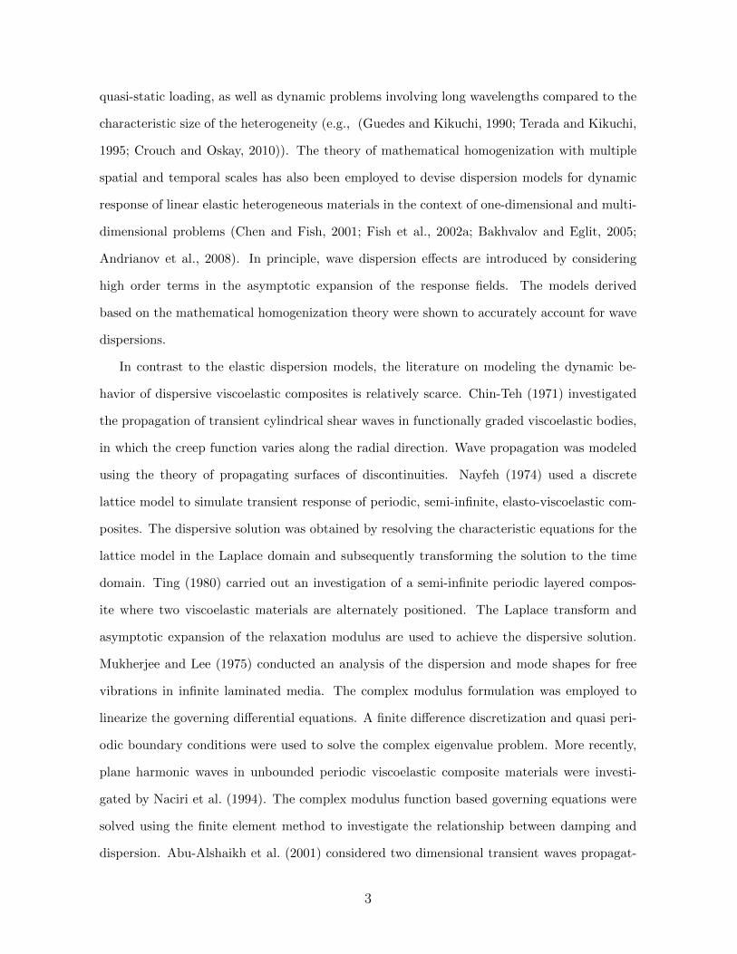
Figure 1: Problems at macroscale and microscale.

micro- and macrostructure size, as well as impulse characteristics. The solution of the nonlocal

homogenization approach is obtained in the semi-analytical form in the Laplace domain and

discrete inverse Laplace transform method is employed to approximate the response fields in

the time domain. The capabilities of the proposed model are verified against the analytical

solution and the classical (local) homogenization model for accuracy and computational cost.

A parametric analysis is conducted to identify the relationship between microstructure and

heterogeneity induced attenuation under high frequency loading.

The remainder of this manuscript is organized as follows: Section 2 presents the description

of the multiscale problem in the time and Laplace domains. Section 3 derives the governing

equations for the nonlocal homogenization model based on the high-order asymptotic expansion

method in the Laplace domain. Section 4 presents the solution methodologies employed to

evaluate the nonlocal and local homogenization models as well as direct analytical evaluation of

the governing equations of motion. This section also provides the implementation of dissipated

energy computation and the discrete inverse Laplace transform method. Section 5 includes

numerical results for heterogeneous beam structures subjected to step and sinusoidal boundary

conditions, and concluding remarks are presented in Section 6.

5

2 Problem Setting

Consider a one-dimensional bimaterial heterogeneous body as illustrated in Fig. 1. The

domain of the body, Ω = [0, L] is formed by the repetition of a locally periodic microstructure,

Θ. The size of the material microstructure is taken to be small compared to the overall size

of the macroscopic domain. Denoting x and y as the position coordinates at the scales of

the macro- and microstructures, respectively, the two scales are related by a small scaling

parameter: y = x/ζ; where, 0 < ζ 1 is the ratio between the characteristic size of the

microstructure and the length of the traveling waves along the heterogeneous body.

Let f ζ(x, t) be an arbitrary response field, which oscillates in space due to fluctuations

induced by the material heterogeneity. We consider the following two scale decomposition of

the original single position coordinate:

f ζ(x, t) = f(x, y(x), t) (1)

where, superscript ζ indicates the dependence of the response field on the microstructural

heterogeneity; and, t denotes time. The spatial derivative of f ζ is computed by the chain rule

as:

f ζ ,x (x, t) = f,x (x, y, t) +1

ζf,y (x, y, t) (2)

where, a subscript followed by a comma denotes differentiation, repeated subscripts denotes

higher order differentiation. The response fields are taken to be spatially periodic throughout

the deformation process:

f(x, y, t) = f(x, y + l, t); ∀x ∈ Ω (3)

in which, l denotes the period of the microstructure in the stretched coordinate system, y

(Fig. 1).

6

2.1 Governing equations in the time domain

In the time domain, the deformation response of the heterogeneous body subjected to

dynamic loading conditions is governed by the momentum balance equation in the form:

σζ,x(x, t) = ρζ(x)uζ,tt(x, t) (4)

in which, σζ and uζ are the stress and displacement fields, respectively; and, ρζ denotes density.

A generalized viscoelastic model described by the Duhamel’s integral is employed to provide

the constitutive response of the material constituents:

σζ(x, t) =

∫ t

0gζ(x, t− τ)εζ,τ (x, τ)dτ (5)

where, gζ is the modulus function; and, εζ denotes the strain field, assuming small strain

kinematics:

εζ(x, t) = uζ,x(x, t) (6)

The dynamic loads are imparted on the heterogeneous body based on prescribed displace-

ments along the boundaries of the domain. We consider the following initial and boundary

conditions:

uζ(x, 0) = u0(x); vζ(x, 0) = v0(x) (7)

uζ(0, t) = 0; uζ(L, t) = u(t) (8)

in which, L is the length of the heterogeneous body; vζ = uζ,t the velocity field; and, u0 , v0

and u are prescribed initial and boundary data.

2.2 Governing equations in the Laplace domain

The particular forms of the generalized viscoelastic constitutive model and the momentum

balance equation permit a simpler description of the governing boundary value problem in the

Laplace domain. In this section, we introduce the key characteristics of the Laplace transform

7

employed in the formulation and recast the governing system of equations in the Laplace

domain.

The Laplace transform of an arbitrary, real valued, time varying function, f ∈ R, is defined

as:

f(s) ≡ L (f(t)) =

∫ ∞0

e−stf(t)dt (9)

where, the Laplace argument, s and the Laplace transform, f , are complex valued (i.e., s ∈ C

and f := C → C). Overbar on a response function indicates the Laplace transform, and the

representation of a function or an equation in the Laplace domain is referred to as associated

function or equation throughout the remainder of this manuscript. The derivative rule for the

Laplace transform is given as:

L (f, tt . . . t︸ ︷︷ ︸n times

(t)) = snf(s)− sn−1f(0)− . . .− f, tt . . . t︸ ︷︷ ︸n−1 times

(0) (10)

and the convolution integral rule is given as:

L

(∫ t

0f1(t− ξ)f2(ξ)dξ

)= L

(∫ t

0f1(ξ)f2(t− ξ)dξ

)= L (f1)L (f2) (11)

Considering a statically undeformed initial condition (i.e., u0(x) = v0(x) = 0), taking the

Laplace transform of the momentum balance equation (Eq. 4) and employing the derivative

rule for the Laplace transform (Eq. 10) yield the associated momentum balance equation:

σζ,x(x, s) = ρζ(x)s2uζ(x, s) (12)

Applying the convolution integral rule (Eq. 11) to the constitutive equation of the vis-

coelastic constituents (Eq. 5) and using Eq. 10 yield the associated constitutive law:

σζ(x, s) = Eζ(x, s)εζ(x, s) (13)

in which, the associated modulus function in the Laplace domain, Eζ , is related to the modulus

8

function, gζ as:

Eζ(x, s) = sL(gζ(x, t)

)(14)

Taking the Laplace transform of the boundary conditions yields the associated boundary

conditions:

uζ(0, s) = 0; uζ(L, s) = u(s) (15)

in which, u is the Laplace transform of the known boundary data, u. The governing equations of

the dynamic response of the heterogeneous body defined in the Laplace domain is summarized

in Box 1.

Given ρζ , Eζ , and u; find uζ ∈ C such that in x ∈ Ω and s ∈ C

Momentum balance: σζ,x(x, s) = ρζ(x)s2uζ(x, s)

Kinematics equation: εζ(x, s) = uζ,x(x, s)

Constitutive equation: σζ(x, s) = Eζ(x, s)uζ,x(x, s); Eζ(x, s) = sL(gζ(x, t)

)Boundary conditions uζ(0, s) = 0; uζ(L, s) = u(s)

Box 1: Governing boundary value problem in the Laplace domain.

The density and modulus are taken to vary as a function of the microscale coordinates

only. For a bimaterial microstructure:

Eζ = E(y, s) =

E1(s) if y ∈ Θ(1)

E2(s) if y ∈ Θ(2)(16)

ρζ = ρ(y) =

ρ1 if y ∈ Θ(1)

ρ2 if y ∈ Θ(2)(17)

where, Θ(1) and Θ(2) are the domains of phases 1 and 2, respectively, such that Θ = Θ(1)∪Θ(2);

and, E1, ρ1 and E2, ρ2 are the material parameters defining the corresponding phases.

9

3 Nonlocal Homogenization

In this section, a nonlocal homogenization model is devised for the dynamic response of

viscoelastic bimaterial composites by applying the mathematical homogenization theory with

multiple spatial scales on the governing equations defined in the Laplace domain. The deriva-

tion follows the procedure originally proposed by Fish et al. (2002b), who devised a nonlocal

homogenization model for linear elastic bimaterial composites by employing the mathematical

homogenization theory in the time domain.

We start by approximating displacement based on the asymptotic expansion of the form:

uζ(x, t) ≡ u(x, y, t) = u0(x, t) + ζu1(x, y, t) + ζ2u2(x, y, t) + ζ3u3(x, y, t) +O(ζ4) (18)

where, u0 denotes the macroscopic displacement field and is independent of the microstructure;

and, ui are spatially oscillatory high-order displacement fields. By linearity of the Laplace

transform, the associated displacement field is also expressed in terms of the asymptotic series:

u(x, y, s) = u0(x, s) + ζu1(x, y, s) + ζ2u2(x, y, s) + ζ3u3(x, y, s) +O(ζ4) (19)

Substituting Eq. 19 into the associated constitutive law (Eq. 13), the stress-strain relation-

ships at any order are obtained as:

O(ζi) : σi (x, y, s) = E(y, s)(ui,x + ui+1,y); i = 0, 1, . . . (20)

Substituting Eq. (19) and the constitutive equations at various orders (Eq. 20) into the

associated momentum balance equation (Eq. 12), the momentum balance equations of orders

10

O(ζ−1) to O(ζ2) are expressed as:

O(ζ−1) : [E(y, s)(u0,x +u1,y )] ,y = 0 (21)

O(1) : ρ(y)u0s2 − [E(y, s)(u0,x +u1,y )] ,x− [E(y, s)(u1,x +u2,y )] ,y = 0 (22)

O(ζ) : ρ(y)u1s2 − [E(y, s)(u1,x +u2,y )] ,x− [E(y, s)(u2,x +u3,y )] ,y = 0 (23)

O(ζ2) : ρ(y)u2s2 − [E(y, s)(u2,x +u3,y )] ,x− [E(y, s)(u3,x +u4,y )] ,y = 0 (24)

Considering the balance equations at the lower two orders (Eqs. 21 and 22) leads to the

classical homogenization model (e.g. Oskay and Fish, 2007). The classical homogenization

model is local in character and valid only when displacement wavelengths are large enough

that the wave reflections along the bimaterial interfaces are negligible. The O(ζ) and O(ζ2)

balance equations introduce high order terms in the resulting homogenized equations, leading

to a nonlocal homogenization model that can account for the dispersion induced by wave

reflections at material microstructure boundaries.

Consider the O(ζ−1) associated boundary value problem (Eq. 21). By linearity, the first

order microscale associated displacement field, u1, is expressed using the following decompo-

sition:

u1(x, y, s) = U1(x, s) +H(y, s)u0,x (x, s) (25)

where, H denotes the first order microscopic influence function providing the oscillatory com-

ponent of u1, whereas U1 denotes the macroscopic contribution of u1. Applying Eq. 25 to

Eq. 21, a linear equilibrium equation for the first order microscopic influence function is ob-

tained:

E(y, s)(1 +H,y),y = 0 (26)

Equation 26 is evaluated by imposing the periodicity, continuity and normality conditions.

The periodicity of the influence function follows from the periodicity of the displacement field:

H(y = 0, s) = H(y = l, s); σ0(x, y = 0, s) = σ0(x, y = l, s) (27)

11

in which, l = l/ζ; and, l is the physical length of the microstructure. The continuity of the

microscale response fields across the bimaterial interfaces are ensured by imposing the following

constraints:

limν→0

H(y = αl + ν+, s)−H(y = αl − ν−, s) = 0 (28)

limν→0

σ0(x, y = αl + ν+, s)− σ0(x, y = αl − ν−, s) = 0 (29)

where, 0 ≤ α ≤ 1 is the volume fraction of phase 1 in the bimaterial microstructure as shown

in Fig. 1. The uniqueness of the influence function is ensured by imposing the normality

condition on the microscale associated displacement field, u1:

〈u1(x, y, s)〉 = U1(x, s)→ 〈H(y, s)〉 = 0 (30)

where, MacCauley brackets, 〈·〉, denote the spatial averaging over the microstructure:

〈f〉 =1

|Θ|

∫Θf(x, y, s)dy (31)

where, |·| is the size of the microstructural domain (i.e., |Θ| = l). Considering the constraints

in Eqs. 27-30, the influence function is evaluated in a closed form as follows,

H(y, s) =

(1− α)(E2(s)− E1(s))

(1− α)E1(s) + αE2(s)

(y − αl

2

); y ∈ Θ(1)

α(E1(s)− E2(s))

(1− α)E1(s) + αE2(s)

(y − (1 + α)l

2

); y ∈ Θ(2)

(32)

The O(1) homogenized equilibrium equation is obtained by applying the averaging operator

(Eq. 31) to the associated balance equation (Eq. 22) . Considering the periodicity of the first

order associated microscopic stress, σ1 yields:

ρ0u0s2 − E0(s)u0,xx = 0 (33)

where, ρ0 and E0(s) denote the homogenized density and homogenized associated modulus

12

function, respectively:

ρ0 ≡ 〈ρ〉 = αρ1 + (1− α)ρ2 (34)

E0(s) = 〈E(y, s)(1 +H,y)〉 =E1(s)E2(s)

(1− α)E1(s) + αE2(s)(35)

Next, we consider the O(1) associated momentum balance equation (Eq. 22). Substituting

Eqs. 25 and 33 into Eq. 22 yields:

E(y, s)(u2,y + U1,x +Hu0,xx)

,y

= (θ(y)− 1)E0 u0,xx (36)

where, θ(y) = ρ(y)/ρ0. By linearity, the second order microscale associated displacement field,

u2 is expressed as:

u2(x, y, s) = U2(x, s) +H(y, s)U1,x(x, s) + P (y, s)u0,xx(x, s) (37)

in which, P (y, s) is the second order microscale influence function. Considering the periodic-

ity, continuity and normality constraints, P is uniquely evaluated by Eq. 36 in closed form.

Employing the closed form expression for the second order microscale influence function and

considering the periodicity of the second order stress field, σ2, the O(ζ) homogenized momen-

tum balance equation is obtained by applying the averaging operator to Eq. 23:

ρ0U1s2 − E0U1,xx = 0 (38)

The third order associated microscale displacement field, u3 is determined using the O(ζ)

momentum balance equation (Eq. 23). Decompositions of the lower order microscale displace-

ment fields (Eqs. 25 and 37) and the homogenized balance equations (Eqs. 33 and 38) at O(1)

and O(ζ) are substituted into Eq. 23 to yield:

E(y, s)(u3,y + U2,x +H(y, s)U1,xx + P (y, s)u0,xxx)

,y

= θ(y)E0(s)H(y, s)− E(y, s)(H + P,y) u0,xxx + (θ(y)− 1)E0(s) U1,xx (39)

13

We consider the following form for the third order associated microscale displacement field:

u3(x, y, s) = U3(x, s) +H(y, s)U2,x +P (y, s)U1,xx +Q(y, s)u0,xxx (40)

where, Q(y, s) is the third order microscale influence function. Analogous to the evaluation of

the lower order influence functions, Q is uniquely determined from the O(ζ) momentum balance

equation provided that the periodicity, continuity and normality conditions are imposed.

The O(ζ2) homogenized momentum balance equation is obtained by applying the averaging

operator to Eq. 24 and utilizing the expressions of P (y, s) and Q(y, s):

ρ0U2s2 − E0U2,xx =

1

ζ2Edu0,xxxx (41)

where,

Ed(s) =[α(1− α)]2(E1ρ1 − E2ρ2)2E0l

2

12ρ20[(1− α)E1 + αE2]2

(42)

Consider the average associated displacement field up to O(ζ3):

U(x, s) = 〈u(x, y, s)〉 = u0(x, s) + ζU1(x, s) + ζ2U2(x, s) +O(ζ3) (43)

Summing the homogenized momentum balance equations at orders O(1), O(ζ), and O(ζ2)

(Eqs. 33, 38 and 41), a governing homogenized balance equation for U is obtained in the

following form:

ρ0s2U − E0U ,xx−EdU ,xxxx = 0 (44)

It is important to note that the dispersive behavior is captured due to the presence of the

last term in Eq. 44. The coefficient Ed introduces a characteristic length term (proportional

to l2). Introducing the dispersive term in the governing equation leads to a fourth order

ordinary differential equation for the evaluation of associated homogenized displacement field,

U(x, s) in the Laplace domain. This is in contrast to the time domain analysis by Fish et al.

(2002b), which leads to a partial differential equation for the evaluation of the homogenized

displacement field in the time domain. Since the governing equation is of the fourth order, the

14

boundary conditions of the original initial boundary value problem provided in Eq. 15 is not

sufficient to uniquely determine U . We therefore consider two additional artificial boundary

conditions:

U,xx(0, s) = 0, U,xxx(L, s) = 0 (45)

The resulting boundary value problem for the homogenized nonlocal response of the hetero-

geneous body subjected to the dynamic loads is summarized in Box 2.

Given ρζ , Eζ , and u; find U ∈ C such that in x ∈ Ω and s ∈ C

Macro-homogenized equilibrium equation: ρ0s2U − E0U ,xx−EdU ,xxxx = 0

Essential boundary conditions: U(0, s) = 0 U(L, s) = u(s)

Additional boundary conditions: U,xx(0, s) = 0 U,xxx(L, s) = 0

Box 2: Governing boundary value problem for the nonlocal homogenization model.

4 Solution Procedures

This section provides the analytical solutions of the nonlocal homogenization model, the

classical homogenization model and the direct single scale boundary value problem. The

computation of the dissipated energy density at a material point in the Laplace domain and

the discrete Laplace transform method employed to describe the computed response fields in

the time domain are presented.

4.1 Homogenization models

The fourth order ordinary differential equation for the nonlocal homogenization model pro-

vided in Box 2 is analytically evaluated by considering the following form for the homogenized

displacement field:

U(x, s) = A(s) sinh(ξx) +B(s) sinh(ηx) (46)

15

in which, the coefficients, A, B, ξ and η are obtained using the boundary conditions as:

A(s) =u(s) η3

(η3 − ξ3) sinh(ξL); B(s) =

u(s) ξ3

(ξ3 − η3) sinh(ηL)(47a)

ξ =

√−E0 +

√E2

0 + 4ρ0Eds2

2Ed; η =

√−E0 −

√E2

0 + 4ρ0Eds2

2Ed(47b)

When homogenization is conducted up to order O(ζ), the formulation described in Section 3

leads to the classical homogenization model governed by the following second order ordinary

differential equation:

ρ0s2u0 − E0u0,xx = 0 (48)

Equation 48 is evaluated analytically using the following form:

u0(x, s) = C(s) sinh(ϕx) (49)

The coefficients C and ϕ are obtained using the boundary conditions as follows:

C(s) =u(s)

sinh (ϕL); ϕ =

sign(Re(s))

V0s; V0 =

√E0

ρ0(50)

where, V0 is the frequency dependent homogenized velocity.

4.2 Original governing equations

Given ρi, Ei and u; find uni ∈ C such that in x ∈ Ω and s ∈ C

Equilibrium equation: Eiuni ,xixi (xi, s) = ρis

2uni (xi, s)

Constitutive equation: σni (xi, s) = Eiuni ,xi (xi, s)

Continuous conditions at interfaces: un1 (αl, s) = un2 (0, s) un2 ((1− α)l, s) = un+11 (0, s)

σn1 (αl, s) = σn2 (0, s) σn2 ((1− α)l, s) = σn+11 (0, s)

Boundary conditions: u11(0, s) = 0 uN2 ((1− α)l, s) = u(s)

Box 3: Summary of the boundary value problem for the nth microstructure

16

In this section, we derive the analytical solution of the original governing boundary value

problem summarized in Box 3. The analytical solution derived in this section is employed

as the reference solution in the numerical simulations that are discussed in the subsequent

sections. The analytical solution is obtained by exploiting the governing equation on each

phase of each microstructure along the heterogeneous body and enforcing continuity across

each bimaterial interface.

We start by numbering microstructures along the beam. At the nth microstructure (n =

1, . . . , N , where N denotes total number of microstructures ). We define two position coor-

dinates x1 and x2 to parameterize the phase domains Ωn1 = [0, αl] and Ωn

2 = [0, (1 − α)l],

respectively. The boundary value problem for each phase of the nth microstructure includ-

ing the continuity conditions for the displacements, uni and stresses, σni at the interfaces are

summarized in Box 3.

The general solution for the equilibrium equation in the boundary value problem is:

uni (x, s) = Ani exp(γix) +Bni exp(−γix) (51)

with,

γi =sign(Re(s))

Vi; Vi =

√Eiρi

(52)

where, Vi is the complex wave velocity of phase i. The displacement and stress fields at the

boundaries of each phase of the nth microstructure read,

un1 (0, s) = An1 +Bn1 , σn1 (0, s) = An1η1 −Bn

1 η1 (53)

un1 (αl, s) = An1ξ1 +Bn1 /ξ1, σn1 (αl, s) = An1η1ξ1 −Bn

1 η1/ξ1 (54)

un2 (0, s) = An2 +Bn2 , σn2 (0, s) = An2η2 −Bn

2 η2 (55)

un2 ((1− α)l, s) = An2ξ2 +Bn2 /ξ2, σn2 ((1− α)l, s) = An2η2ξ2 −Bn

2 η2/ξ2 (56)

17

with,

ξ1 = exp (γ1αl) , ξ2 = exp (γ2(1− α)l) (57)

η1 = E1γ1, η2 = E2γ2 (58)

The boundary and continuity conditions of displacement and stress fields are used to determine

the unknowns Ani and Bni :

Boundary conditions: A11 +B1

1 = 0 (59)

AN2 ξ2 +BN2 /ξ2 = u(s) (60)

Displacement continuities: An1ξ1 +Bn1 /ξ1 = An2 +Bn

2 (61)

An2ξ2 +Bn2 /ξ2 = An+1

1 +Bn+11 (62)

Stress continuities: An1η1ξ1 −Bn1 η1/ξ1 = An2η2 −Bn

2 η2 (63)

An2η2ξ2 −Bn2 η2/ξ2 = An+1

1 η1 −Bn+11 η1 (64)

Equations 59 - 64 are expressed in the following matrix form:

MX = F (65)

18

where,

M(4N×4N) =

1 1

ξ1 1/ξ1 −1 −1 0

η1ξ1 −η1/ξ1 −η2 η2

ξ2 1/ξ2 −1 −1

η2ξ2 −η2/ξ2 −η1 η1

. . .

ξ1 1/ξ1 −1 −1

0 η1ξ1 −η1/ξ1 −η2 η2

ξ2 1/ξ2

(66)

and,

F(4N×1) = [0, 0, . . . , 0, u(s)]T (67)

X(4N×1) =[A1

1, B11 , A

12, B

12 . . . , A

N1 , B

N1 , A

N2 , B

N2

]T(68)

Evaluating Eq. 65 provides the analytical (reference) solution. To compare the homogenized

response computed by the homogenization models described in Section 4.1, we average the

computed displacement field over each microstructure:

Un(s) =1

l

(∫ αl

0un1 (x, s)dx+

∫ (1−α)l

0un2 (x, s)dx

)(69)

Substituting equation 51 into 69:

Un(s) =1

l

[An1 (ξ1 − 1)−Bn

1

(1

ξ1− 1

)]1

γ1+

[An2 (ξ2 − 1)−Bn

2

(1

ξ2− 1

)]1

γ2

(70)

The dimension of the matrix M is 4N × 4N , which indicates that the computational cost

of the reference solution increases as a function of the number of microstructures along the

heterogeneous body. Computational time could therefore prohibit the evaluation of problems

with a large number of microstructures. The analytical solution is only employed for the

19

verification of the nonlocal homogenization model.

4.3 Inverse Laplace transform

Since all the associated fields are derived in the Laplace domain, it is necessary to trans-

form the response fields into the time domain. The numerical inverse Laplace Transform

Method (Brancik, 1999), which is based on Fast Fourier Transform and the ε-error algo-

rithm (Macdonald, 1964) is used for transforming the response fields to the time domain. The

inverse Laplace Transform is defined as,

f(t) =1

2πi

∫ c+i∞

c−i∞F (s)estds (71)

with the assumptions that, |f(t)| ≤ Keβt, where, K is real and positive; t > 0; and Re(s) > β.

The numerical inverse Laplace transform is computed by Nv-term truncation, F(Nv) of the

transformed function values of F (s), with the subscript Nv denoting the dimension of the

vector:

f(Mv) = C(Mv)

2Re[E (FFT(F(Nv)))

]− F0(Mv)

(72)

where, denotes the Hadamard product of matrices, e.g. the element-by-element product;

E (·) represents the ε-error algorithm, and F0(Mv) is a Mv-element constant vector of c which

can be computed as,

c = β − Ω

2πlnEr (73)

Ω = π(1− 1/Mv)/tm (74)

where tm = (Mv − 1)Ts and Mv = Nv/2. Ts is the sampling period in the time domain, Er

the desired relative error, and:

C(Mv)(k) =Ω

2πexp(ckTs) (75)

F(Nv)(n) = F (c− inΩ) n = 0, 1, . . . , Nv − 1 (76)

20

A more detailed description of the inverse Laplace transform method is presented by Brancik

(1999).

4.4 Dissipated energy

The rate of dissipated energy density for the viscoelastic material model using the Duhamel’s

integral takes the following form (Fung, 1965):

Wd(x, y, t) =

∫ t

0

∫ t

0−g(x, y, 2t− τ1 − τ2)ε,τ1(x, y, τ1)ε,τ2(x, y, τ2)dτ1dτ2 (77)

Equation 77 requires the computation of strain field in the time domain. In the Laplace

domain, the associated macroscopic strain, ε is related to the associated displacement field as

follows,

ε(x, y, s) = u,x (78)

Substituting Eq. 19 and the linearizions of u1, u2, and, u3 (i.e. Eqs. 25, 37) and 40, into Eq. 78,

we can simplify the expression for associated strain:

ε(x, y, s) = (1 +H,y)U,x + ζ(H + P,y)U,xx + ζ2(P +Q,y)U,xxx +O(ζ3) (79)

in which, the localization functions, (1 + H,y), (H + P,y) and (P + Q,y) are readily available

through differentiation of the influence functions and provided in Appendix A.

The reference solution provides the associated strain of phase i in microstructure Ωni as:

εni (xi, y, s) = Ani γi exp(γixi)−Bni γi exp(−γixi) i = 1, 2 and n = 1, 2, ..., N (80)

The rate of dissipated energy density is evaluated by inverting the associated strain and sub-

stituting it into the real time domain using the numerical inverse Laplace transform.

21

Table 1: Viscoelastic material parameters for polyurea (Amirkhizi et al., 2006).

k1 [MPa] k2 [MPa] k3 [MPa] k4 [MPa] ke [MPa]37.8918 75.5328 161.0112 194.5216 44.8

q1 [ms] q2 [ms] q3 [ms] q4 [ms] ρ [kg/m3]463.4 0.06407 1.163× 10−4 7.321× 10−7 1070

5 Numerical Examples

A series of simulations have been conducted to assess the validity of the proposed nonlo-

cal homogenization model and investigate the energy dissipation characteristics of bimaterial

composites as a function of microstructural configuration. The capabilities of the model is

verified against the analytical solution of the original single scale boundary value problem and

the classical local homogenization model.

The material moduli function that represents the material properties at the scale of mi-

crostructure is modeled as:

g(y, t) =

E1 if y ∈ Θ(1)

ke +

n∑i=1

kie−t/qi if y ∈ Θ(2)

(81)

where n is number of Prony series. In all cases below, the first phase is taken to be elastic,

whereas the second phase is viscoelastic, modeled by a Prony series approximation. The

viscoelastic material idealizes the response of the polyurea material. The material properties

of polyurea is provided by Amirkhizi et al. (2006) and summarized in Table 1. Applying the

Laplace transform to the modulus function yields:

E(y, s) =

E1 if y ∈ Θ(1)

E2(s) = ke +

n∑i=1

kis

s+ 1qi

if y ∈ Θ(2)(82)

The dissipated energy computations are conducted by taking advantage of the Prony series

22

ũ(t)

step function

t[s]

ũ(t)= M0sin(2πθt)

M0

t[s]

(a) (b)

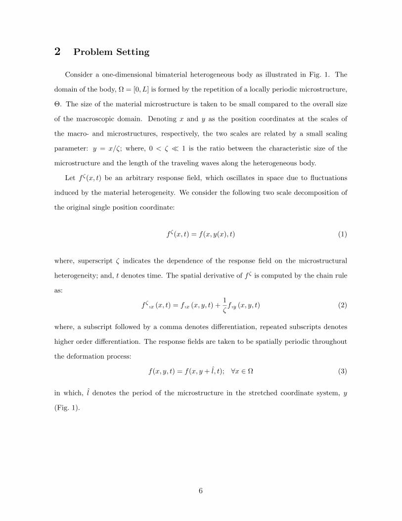
Figure 2: Applied boundary conditions.

approximation. The rate of dissipated energy at the viscoelastic phase is expressed as:

Wd(x, t) =

n∑i=1

kiqiεid(x, t)ε

id(x, t) (83)

where,

εid(x, t) =

∫ t

0exp (−(t− τ)/qi) ε dτ (84)

5.1 Model verification: dispersion and dissipation

In this section, we verify the capability of the nonlocal homogenization model (NHM) in

capturing the energy dissipation and dispersion under dynamic loadings. The response of

NHM is compared to the classical homogenization model (CHM) and the analytical solution

of the reference model (AS). The ratio of the macroscopic and microscopic domain sizes (i.e.,

N) is set as 40. The modulus of the elastic phase (phase 1) is taken as 1 GPa, and the two

phases have equal volume fractions (i.e., α = 0.5).

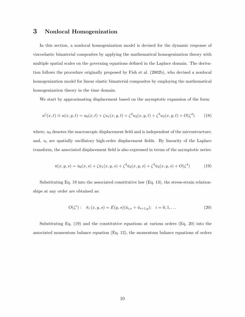
First, we consider the response when the end of the bar is subjected to step loading with

magnitude M0 as illustrated Fig. 2a. We evaluate the response of the bars with four different

density contrast in the microstructure (i.e., φ = ρ1/ρ2 = 1, 2, 5, 10). The normalized displace-

ment histories as a function of the normalized time (i.e., t/T where, T denotes the observation

duration) are shown in Fig. 3 for the four density ratios as computed using NHM, CHM and

the reference solutions. The displacement histories are recorded at 0.82L distance from the

fixed end of the bar. The “cycles” observed in Fig. 3 are due to the repeated reflections of the

wave at the fixed and loaded boundaries of the domain. In Figs. 3a-d, the distance between

23

the displacement peak and trough at each cycle reduces, indicating progressive attenuation

of the wave. At the asymptote of complete attenuation, the normalized displacement at the

control point approaches 0.82. This corresponds to the uniform strain state induced by a

quasi-statically applied unit displacement at the loaded end. At all density ratios, the results

indicate good agreement between the nonlocal homogenization approach and the reference

solution. Figures 3a-d illustrate that the wave dispersion increases with the density ratio in

the microstructure. While the nonlocal model accurately accounts for the wave dispersion at

high density ratios, the classical homogenization model fails to capture the wave dispersions.

Yet, the dissipation patterns are accurately captured by CHM, which indicates that the atten-

uation induced by wave dispersion is relatively small. In other words, the dispersion induced

attenuation can only be captured by taking account of the higher order derivative term in

NHM, however the viscoelastic dissipation resulting from the viscoelastic modulus is included

in both the NHM and CHM.

In the simulations displayed in Fig. 3, the density ratios of (i.e., φ = 1, 2, 5, 10) are set by

increasing the density of the elastic constituent, ρ1, while keeping the density of the viscoelastic

constituent, ρ2, constant. The density of the homogenized constituent, ρ0, in Eq. 34 therefore

increases as φ is increased, leading to lower wave velocity of the homogenized domain and

slower propagation. The effect of dispersion induced internal scattering on the propagation

rate at high density ratios is relatively minor. This is because the CHM model is able to

capture the slower propagation of the wave at high density ratios accurately, despite missing

the dispersion effects.

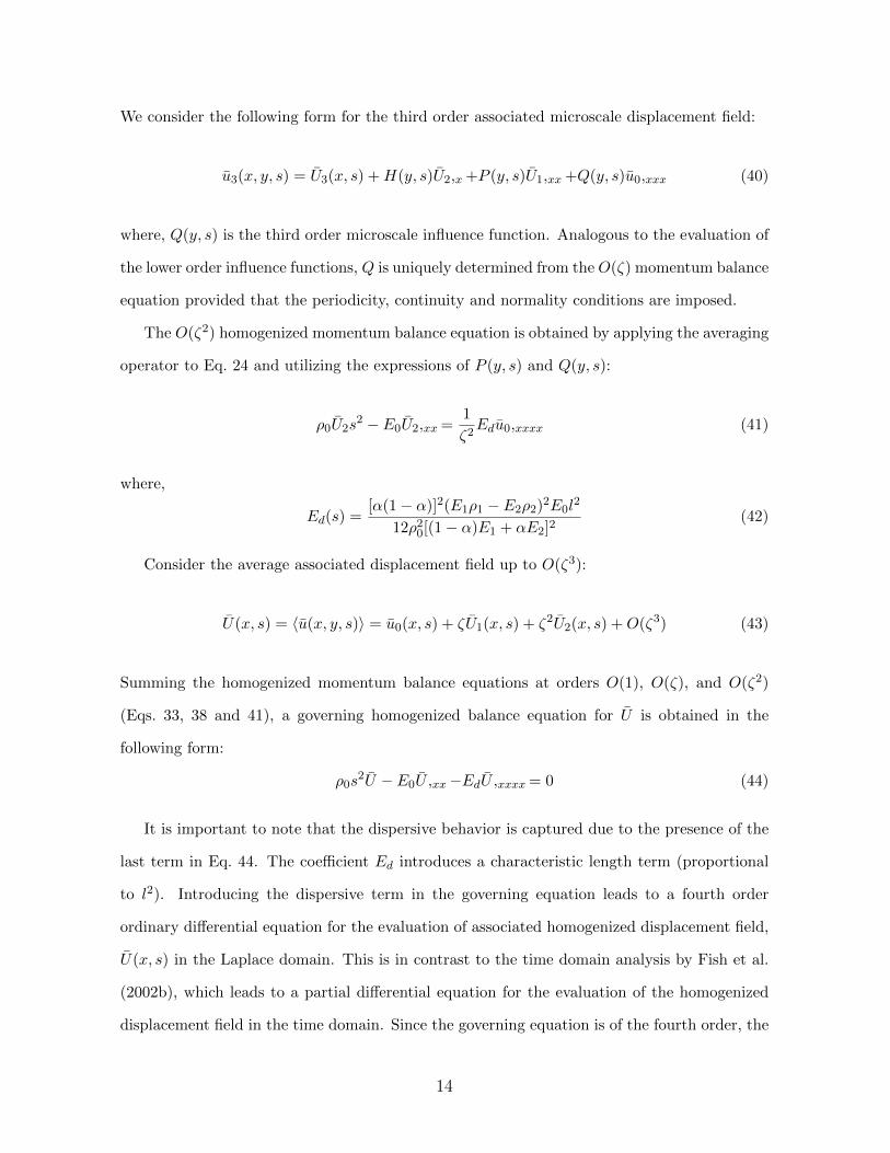
Next, we investigate the response of the bar when subjected to sinusoidal loading as il-

lustrated in Fig. 2b. The applied loadings is parameterized by the magnitude, M0 and the

frequency, θ. The density ratio, φ of the heterogeneous bar is set to 10. Figure 4 shows the

normalized displacement history for identical heterogeneous bars vibrating at four different

frequencies ( θ = 10, 30, 50, and 70 Hz) recorded at 0.82L distance from the fixed end of the

specimen. At relatively low frequency loading (e.g., θ = 10 Hz), the classical and the nonlocal

homogenization models capture the response reasonably accurately, with the exception of the

phase shift and accompanying reduction in the peak amplitude originating from the wave re-

24

0 0.1 0.2 0.3 0.4 0.5 0.6 0.7 0.8 0.9 1-0.2

00.20.40.60.81

1.2U

/M0

0 0.1 0.2 0.3 0.4 0.5 0.6 0.7 0.8 0.9 1-0.2

00.20.40.60.81

1.2

0 0.1 0.2 0.3 0.4 0.5 0.6 0.7 0.8 0.9 1-0.2

00.20.40.60.81

1.2

U/M

0

t/T

ASCHMNHM

0 0.1 0.2 0.3 0.4 0.5 0.6 0.7 0.8 0.9 1-0.2

00.20.40.60.81

1.2

t/T

(a) φ=1 (b) φ=2

(c) φ=5 (d) φ=10

Figure 3: Displacement histories under different density ratios when subjected to steploading.

0 0.2 0.4 0.6 0.8 1-2-1

0

1

2

U/M

0

0 0.2 0.4 0.6 0.8 1-2-1

0

1

2

0 0.2 0.4 0.6 0.8 1-2-1

0

1

2

t/T

U/M

0

0 0.2 0.4 0.6 0.8 1-2-1

0

1

2

t/T

NHMCHMAS

(a) θ=10 (b) θ=30

(c) θ=50 (d) θ=70

Figure 4: Displacement histories under different loading frequencies when subjected tosinusoidal loading.

25

0 0.2 0.4 0.6 0.8 10

250

500

750

1000

0 0.2 0.4 0.6 0.8 10

25

50

75

100W

d /W0

0 0.2 0.4 0.6 0.8 10

1000

2000

3000

t/T0 0.2 0.4 0.6 0.8 1

0

1

2

34

t/T

(a) θ=10 (b) θ=30

(c) θ=50 (d) θ=70

NHMCHMAS

Wd /W

0

Figure 5: Dissipated energy density histories under different loading frequencies.

flections at the fixed end. At higher frequency loading (θ = 30− 50 Hz), the attenuation due

to heterogeneity induced wave dispersions becomes significantly more pronounced since the

shorter wavelength events reflect at the bimaterial interfaces, dissipating energy in the viscous

phase. At the highest considered frequency (i.e., θ = 70 Hz), the wave dissipates within a short

distance from the applied loading. CHM clearly cannot predict such a attenuation phenomena

as apparent in Fig. 4. At high frequency loading, the microscopic dynamics is critical for

accurate modeling of dispersive behavior. These observations are reinforced by the dissipated

energy density comparison computed at the inspection point on the bar (0.82L distance from

the fixed end of the specimen) under sinusoidal loadings as shown in Figure 5. The energy

dissipation prediction by NHM is in reasonable agreement with the reference solution for the

entire applied loading frequency range, whereas CHM is applicable only for low frequency load-

ings. The overprediction of dissipation density by CHM at high frequencies at the inspection

location reflects the presence of spurious high amplitude waves traveling through the material.

The nonlocal model dissipates all high frequency waves prior to reaching the inspection point.

In addition to the favorable accuracy of the nonlocal homogenization model demonstrated

above, it is computationally significantly more efficient compared to the reference simulation.

While NHM employs a single equilibrium equation in the evaluation of the dynamics response,

26

the reference model requires the solution of a 4N × 4N system of equations leading to signifi-

cant computational cost. For instance, when 500 microstructures are included in the problem

(i.e., N = 500), the computational time required to solve the reference problem is three orders

of magnitude larger than the nonlocal model. Such an analysis required approximately two

minutes computation time for the nonlocal homogenization model using a single workstation,

whereas several days were required to complete the same analysis based on the reference solu-

tion. This drawback makes using the analytical solution for simulating responses in structures

having a large number of microstructures intractable, and the nonlocal homogenization is fa-

vorable compared to the CHM and the reference solution by providing accurate predictions at

both scales while maintaining satisfactory time efficiency.

5.2 Effect of microstructure on energy dissipation

In this section, we investigate the dispersive-dissipative wave propagation response for the

effect of microstructure on the energy dissipation characteristics. A steel-polyurea composite

bar is considered. The material properties of the viscoelastic polyurea phase are summarized

in Table 1. The density and modulus of the elastic steel phase are set to ρ1 = 7847 kg/m3

and E1 = 200 GPa, respectively. The bar is subjected to a sinusoidal loading with the loading

frequency of θ = 80 Hz. The ratio of the macroscopic and microscopic domain sizes is set as

N = 20. The dynamics response of the composite is investigated for six microstructural con-

figurations (α = 0.1, 0.25, 0.4, 0.6, 0.75 and 0.9). Nonlocal homogenization model is employed

to predict the responses.

Figure 6 displays the normalized displacement profiles as a function of time and position

for the duration of the dynamic loading. When the microstructure consists largely of the

polyurea or the steel phase (i.e., α = 0.1 and α = 0.9, respectively), wave propagation extends

throughout the length of the bar. The energy dissipation in the polyurea dominated bar (i.e.,

α = 0.1) is observed at further distance from the excited boundary, whereas small amount of

dissipation is observed in the steel dominated bar (i.e., α = 0.9). For intermediate configura-

tions with comparable polyurea and steel volume fractions (i.e., α = 0.25, 0.4, 0.6 and 0.7), the

propagation attenuates within approximately a tenth of the bar, pointing to strong dissipation

27

0.7 0.8 0.9 100.250.50.751

−2−1

012

t/T

U/M

0

x/L

(a) α = 0.1

0.7 0.8 0.9 1

00.250.50.751−2−1

012

U/M

0

x/Lt/T

(b) α = 0.25

0.7 0.8 0.9 100.250.50.751

−2−1

012

t/T

U/M

0

x/L

(c) α = 0.4

0.7 0.8 0.9 100.250.50.751

−2−1

012

U/M

0

x/Lt/T

(d) α = 0.6

0.7 0.8 0.9 1

00.250.50.751−2−1

012

U/M

0

x/Lt/T

(e) α = 0.75

0.7 0.8 0.9 1

00.250.50.751−2−1

012

U/M

0

x/Lt/T

(f) α = 0.9

Figure 6: Macrostructural analysis of the displacements for different microstructures.

28

characteristics activated by the microstructural configuration. The results indicate that the

energy dissipation characteristics of the composite steel-polyurea system with balanced vol-

ume fractions are even more favorable than configurations dominated by the viscous polyurea

phase.

6 Conclusion

This manuscript presented a nonlocal dispersive model for the dynamic response of vis-

coelastic heterogeneous materials. The proposed model is based on the mathematical ho-

mogenization theory with multiple spatial scales applied in the Laplace domain. Asymptotic

expansions of the response fields of up to fourth order are included in the homogenization

formulation to account for the wave dispersions induced by the microstructural heterogeneity.

Numerical verifications indicate that the proposed nonlocal model accurately accounts for the

dispersion and dispersion induced attenuation under a wide range of loading and material

parameters, which cannot be modeled using the classical homogenization models. In addition,

the nonlocal homogenization model provides a high level of computational efficiency by elimi-

nating the temporal and microscopic coordinates. The nonlocal model is used to demonstrate

that the microstructural configuration may have a significant impact on the energy dissipation

characteristics of heterogeneous materials under dynamic loading conditions.

From the modeling point of view, additional challenges remain that will be addressed in the

near future. The model is developed in the context of one-dimensional problems, and will be

generalized to the higher dimensions. Extending the proposed approach to higher dimensions

requires computational methods rather than the analytical solutions derived in this manuscript,

due to the complexity of microstructures. Extending the model to higher dimensions naturally

opens the possibility of exploring a wider parameter space of microstructure design for devising

microstructural configurations with favorable energy dissipation characteristics.

29

Acknowledgments

The financial support of the National Science Foundation, CMMI Hazard Mitigation and

Structural Engineering program (Grant #:0856168) is gratefully acknowledged.

Bibliography

I. Abu-Alshaikh, D. Turhan, and Y. Mengi. Propagation of transient out-of-plane shear waves

in viscoelastic layered media. Int. J. Mech. Sci., 43:2911–2928, 2001.

A. V. Amirkhizi, J. Isaacs, J. McGee, and S. Nemat-Nasser. An experimentally-based viscoelas-

tic constitutive model for polyurea, including pressure and temperature effects. Philos. Mag.,

86:5847–5866, 2006.

I. V. Andrianov, V. I. Bolshakov, V. V. Danishevs’ kyy, and D. Weichert. Higher order

asymptotic homogenization and wave propagation in periodic composite materials. Proc.

R. Soc. Lond. A, 464:1181–1201, 2008.

N. S. Bakhvalov and M. E. Eglit. Equations of higher order of accuracy describing the vibra-

tions of thin plates*. J. Appl. Math. Mech., 69(4):593–610, 2005.

N. S. Bakhvalov and G. Panasenko. Homogenisation: averaging processes in periodic media

(mathematical problems in the mechanics of composite materials). Recherche, 67:02, 1989.

T. Bennett, I. M. Gitman, and H. Askes. Elasticity theories with higher-order gradients of

inertia and stiffness for the modelling of wave dispersion in laminates. Int. J. Fract., 148:

185–193, 2007.

A. Bensoussan, J. L. Lions, and G. Papanicolaou. Asymptotic analysis for periodic structures,

volume 5. North Holland, Amsterdam, 1978.

L. Brancik. Programs for fast numerical inversion of laplace transforms in matlab language

environment. Sbornik 7. Proc. Matlab 99, Prague, pages 27–39, 1999.

30

W. Chen and J. Fish. A dispersive model for wave propagation in periodic heterogeneous

media based on homogenization with multiple spatial and temporal scales. ASME J. Appl.

Mech., 68:153–161, 2001.

S. Chin-Teh. Transient rotary shear waves in nonhomogeneous viscoelastic media. Int. J.

Solids Struct., 7:25–37, 1971.

E. Cosserat and F. Cosserat. Theorie des Corps Deformables. Hermann & Fils, Paris, France.,

1909.

R. Crouch and C. Oskay. Symmetric mesomechanical model for failure analysis of heteroge-

neous materials. Int. J. Multiscale Comput. Eng., 8(5):447–461, 2010.

J. Engelbrecht, A. Berezovski, F. Pastrone, and M. Braun. Waves in microstructured materials

and dispersion. Philos. Mag., 85:4127–4141, 2005.

C. Eringen and E. S. Suhubi. Nonlinear theory of micro-elastic solids II. Int. J. Eng. Sci., 2:

189–203, 1964.

J. Fish and W. Chen. Higher-order homogenization of initial/boundary-value problem. J.

Eng. Mech., 127:1223–1230, 2001.

J. Fish, W. Chen, and G. Nagai. Non-local dispersive model for wave propagation in hetero-

geneous media: multi-dimensional case. Int. J. Numer. Methods Eng., 54:347–363, 2002a.

J. Fish, W. Chen, and G. Nagai. Non-local dispersive model for wave propagation in hetero-

geneous media: one-dimensional case. Int. J. Numer. Methods Eng., 54:331–346, 2002b.

Y. Fung. Foundations of solid mechanics. Prentice Hall, Englewood Cliffs, New Jersey, 1965.

S. Gonella, M. S. Greene, and W.K. Liu. Characterization of heterogeneous solids via wave

methods in computational microelasticity. J. Mech. Phys. Solids, 59:959–974, 2011.

J. M. Guedes and N. Kikuchi. Preprocessing and postprocessing for materials based on the

homogenization method with adaptive finite element methods. Comput. Meth. Appl. Mech.

Eng., 83(2):143–198, 1990.

31

Y. Jiangong. Viscoelastic shear horizontal wave in graded and layered plates. Int. J. Solids

Struct., 48:2361–2372, 2011.

J. R. Macdonald. Accelerated convergence, divergence, iteration, extrapolation, and curve

fitting. J. Appl. Phys., 35:3034–3041, 1964.

R. D. Mindlin. Micro-structure in linear elasticity. Arch. Ration. Mech. Anal., 16:51–78, 1964.

S. Mukherjee and E. H. Lee. Dispersion relations and mode shapes for waves in laminated

viscoelastic composites by finite difference methods. Comput. Struct., 5:279–285, 1975.

T. Naciri, P. Navi, and A. Ehrlacher. Harmonic wave propagation in viscoelastic heterogeneous

materials part i: Dispersion and damping relations. Mech. Mater., 18:313–333, 1994.

A. H. Nayfeh. Discrete lattice simulation of transient motions in elastic and viscoelastic

composites. Int. J. Solids Struct., 10:231–242, 1974.

C. Oskay and J. Fish. Eigendeformation-based reduced order homogenization for failure anal-

ysis of heterogeneous materials. Comput. Meth. Appl. Mech. Eng., 196:1216–1243, 2007.

A. V. Porubov, E. L. Aero, and G. A. Maugin. Two approaches to study essentially nonlinear

and dispersive properties of the internal structure of materials. Phys. Rev. E, 79:046608,

2009.

M. B. Rubin, P. Rosenau, and O. Gottlieb. Continuum model of dispersion caused by an

inherent material characteristic length. J. Appl. Phys., 77:4054–4063, 1995.

E. Sanchez-Palencia. Non-homogeneous media and vibration theory, volume 127. Springer-

Verlag, Berlin, 1980.

F. Santosa and W. W. Symes. A dispersive effective medium for wave propagation in periodic

composites. SIAM J. Appl. Math., 51:984–1005, 1991.

K. Terada and N. Kikuchi. Nonlinear homogenization method for practical applications. In

S. Ghosh and M. Ostoja-Starzewski, editors, Computational Methods in Micromechanics,

volume AMD-212/MD-62, pages 1–16. ASME, 1995.

32

T. C. T. Ting. The effects of dispersion and dissipation on wave propagation in viscoelastic

layered composities. Int. J. Solids Struct., 16:903–911, 1980.

L. Tsai and V. Prakash. Structure of weak shock waves in 2-d layered material systems. Int.

J. Solids Struct., 42:727–750, 2005.

Z.-P. Wang and C. T. Sun. Modeling micro-inertia in heterogeneous materials under dynamic

loading. Wave Motion, 36:473–485, 2002.

A Higher order terms

The localization functions: 1+H,y(y, s), H(y, s)+P,y(y, s) and P (y, s)+Q,y(y, s) in Eq. 79

are derived and shown as follows:

1 +H1,y(y, s) =E0

E1(A.1)

1 +H2,y(y, s) =E0

E2(A.2)

H1(y, s) + P1,y(y, s) =E0(1− α)(ρ1 − ρ2)

2ρ0E1(2y − αl) (A.3)

H2(y, s) + P2,y(y, s) =E0α(ρ1 − ρ2)

2ρ0E2((1 + α)l − 2y) (A.4)

P1(y, s) +Q1,y(y, s) =E2

0(1− α) [E1(−2ρ1 + ρ0) + E2(ρ1 + ρ2 − ρ0)]

2ρ0E12E2

(y2 − αly)− E30(1− α)αl2

12ρ0E13E2

2 ·[((1− α)2E1

2 + α2E22)

(ρ0 − ρ1 − ρ2)− E1E2

((2α3 − 4α2 + α)ρ1 − (2α3 − 2α2 − α+ 1)ρ2

)](A.5)

P2(y, s) +Q2,y(y, s) =E2

0α [E1(ρ0 − ρ1 − ρ2) + E2(2ρ2 − ρ0)]

2ρ0E1E22 ((l + αl)y − y2) +

E30αl

2

12ρ0E12E2

3 ·[(−1− 3α+ 3α2 + α3

)(ρ0 − ρ1 − ρ2)E1

2 + α2((

1 + 4α+ α2)ρ1 −

(6 + 5α+ α2

)ρ2

)E2

2

+E1E2

((α+ 7α2 − 6α3 − 2α4)ρ1 + (−1− 4α+ α2 + 8α3 + 2α4)ρ2

)](A.6)

33