A Newtonian Development of the Mean-Axis Dynamics

with Example and Simulation

A THESISSUBMITTED TO THE FACULTY OF THE GRADUATE SCHOOL

OF THE UNIVERSITY OF MINNESOTABY

Sally Ann Keyes

IN PARTIAL FULFILLMENT OF THE REQUIREMENTSFOR THE DEGREE OFMASTER OF SCIENCE

Peter J. Seiler

May 2017

© Sally Ann Keyes 2017

Acknowledgments

I would like to thank my family and friends for their unwavering support and encourage-ment. My gratitude for them is immeasurable.

I would like to thank my advisor, Peter Seiler Jr., for all the time and effort he has spentteaching me about research and mentoring me. I would also like to thank him for the manyoccasions I came to his office with an idea I had yet to figure out how to explain. Pete wasalways patient, trusted in my ideas and intuition, and never failed to help me come up withan explanation I could share with others.

I would like to thank David Schmidt for his time and expertise as I have explored the fieldof the mean axes. His influence has impacted my research tremendously and helped me tomake meaningful connections to the work of the flight dynamics community.

I would like to thank NASA for the generous funding that has made the Performance Adap-tive Aeroelastic Wing a reality. This work was carried out as a part of that project and wasfunded under NASA NRA, ”Lightweight Adaptive Aeroelastic Wing for Enhanced Perfor-mance Across the Flight Envelope,” NRA NNX14AL36A, with Mr. John Bosworth servingas the Technical Monitor.

I would like to thank the University of Minnesota for the College of Science and Engineer-ing Graduate Fellowship. The fellowship has helped to make my research possible and hasgiven me the opportunity to freely pursue my ideas.

Finally, I would like to acknowledge the Kenneth G. and Rosemary R. Anderson Fellowshipas well as the John A. and Jane Dunning Copper Fellowship. Both of these fellowships haveallowed me extra freedom to commit to my research and academic work.

i

Dedication

To my parents, Jimmy and Cindy, for their endless support.

ii

Abstract

Mean-axis models of flight dynamics for flexible aircraft are being utilized more frequentlyin recent dynamics and controls research. The equations of motion resulting from themean-axis formulation are frequently developed with Lagrangian mechanics. In addition,the models are typically simplified using assumptions regarding the effects of the elasticdeformation. Although widely accepted in the literature, the formulation and assumptionsmay be confusing to a user outside of the flight dynamics field (such as a controls engineer).In this thesis, the equations of motion are derived from first principles utilizing Newtonian,rather than Lagrangian, mechanics. In this framework, the formulation offers a new setof insights into the equations of motion and explanations for the assumptions. A three-lumped-mass idealization of a rolling flexible aircraft is presented as an example of themean-axis equations of motion. The example is also used to investigate the effects ofcommon simplifying assumptions. The equations of motion are also developed without anysuch assumptions, and simulation results allow for a comparison of the exact and simplifieddynamics.

iii

Contents

List of Tables vii

List of Figures viii

Chapter 1 Introduction 1

Chapter 2 The Mean Axes 3

2.1 Notation and Problem Formulation . . . . . . . . . . . . . . . . . . . . . . 3

2.2 Mean-Axis Constraints . . . . . . . . . . . . . . . . . . . . . . . . . . . . 6

2.3 Translation of the Mean Axes . . . . . . . . . . . . . . . . . . . . . . . . . 7

2.4 Rotation of the Mean Axes . . . . . . . . . . . . . . . . . . . . . . . . . . 9

Chapter 3 Linear Deformation and the Mean Axes 13

3.1 Equations of Motion in an Inertial Frame . . . . . . . . . . . . . . . . . . . 13

3.2 Equations of Motion in a Body-Reference Frame . . . . . . . . . . . . . . 16

3.3 Equations of Motion in the Mean-Axis Frame . . . . . . . . . . . . . . . . 19

3.4 Final Equations of Motion . . . . . . . . . . . . . . . . . . . . . . . . . . 25

3.5 Newtonian versus Lagrangian Derivation . . . . . . . . . . . . . . . . . . . 27

iv

Chapter 4 Three Mass Example 29

4.1 Introduction to the Three Mass Example . . . . . . . . . . . . . . . . . . . 29

4.2 The General Equations of Motion . . . . . . . . . . . . . . . . . . . . . . 30

4.3 Equations of Motion in Terms of Vibration Modal Coordinate . . . . . . . 32

4.4 The Decoupled Equations . . . . . . . . . . . . . . . . . . . . . . . . . . . 34

Chapter 5 Three Mass Simulation and Analysis 35

5.1 Simulation Setup . . . . . . . . . . . . . . . . . . . . . . . . . . . . . . . 35

5.2 Trajectory Analysis . . . . . . . . . . . . . . . . . . . . . . . . . . . . . . 36

5.3 Coupling and Forcing Analysis . . . . . . . . . . . . . . . . . . . . . . . . 39

5.4 Insight from the Three Mass Example . . . . . . . . . . . . . . . . . . . . 40

Chapter 6 Conclusions and Future Work 42

Bibliography 44

Appendix A Appendices 46

A.1 Useful Facts of Modal Matrices . . . . . . . . . . . . . . . . . . . . . . . 46

A.2 Simplification of Translational Dynamics in Mean Axes . . . . . . . . . . . 48

A.3 Simplification of Rotational Dynamics in Mean Axes . . . . . . . . . . . . 49

A.4 Internal Angular Momentum and its Derivative in Mean Axes . . . . . . . . 51

A.5 Simplification of Elastic Dynamics in Mean Axes . . . . . . . . . . . . . . 52

A.6 Three Mass Example Supplementary Material . . . . . . . . . . . . . . . . 53

A.6.1 Numerical Values for the Three Mass Structure . . . . . . . . . . . 53

v

A.6.2 Linearized Stiffness . . . . . . . . . . . . . . . . . . . . . . . . . 54

A.6.3 Numerical Values for the Three Mass Aerodynamics . . . . . . . . 55

vi

List of Tables

5.1 RMS Error for Three Mass Example Solutions . . . . . . . . . . . . . . . . 38

5.2 Numerical Comparison of Neglected Terms to Forcing Terms . . . . . . . . 39

A.1 Numerical Values for the Three Mass Structure . . . . . . . . . . . . . . . 54

A.2 Numerical Values for the Three Mass Aerodynamics . . . . . . . . . . . . 55

vii

List of Figures

2.1 Left: Notation for system of particles in an inertial (x, y, z) frame. Right:Notation for system using a body (x′, y′, z′) frame. . . . . . . . . . . . . . 4

3.1 Position of particle i with si and δi denoting the undeformed position anddeformation in an inertial frame. . . . . . . . . . . . . . . . . . . . . . . . 14

3.2 Position of particle i with si and δi denoting the undeformed position anddeformation in an the body-reference frame. . . . . . . . . . . . . . . . . . 17

4.1 Lumped 3 Mass Structure. . . . . . . . . . . . . . . . . . . . . . . . . . . 29

4.2 Variables describing the 3-Body Problem. . . . . . . . . . . . . . . . . . . 30

4.3 Bending and translational deflection. . . . . . . . . . . . . . . . . . . . . . 32

5.1 Control Surface Input to Generate Large but Expected Conditions. . . . . . 37

5.2 Bank and Deflection Trajectories . . . . . . . . . . . . . . . . . . . . . . . 37

5.3 Center of Mass Trajectory . . . . . . . . . . . . . . . . . . . . . . . . . . 38

5.4 Coupling Term Comparison . . . . . . . . . . . . . . . . . . . . . . . . . 40

viii

Chapter 1

Introduction

The objective of this work is to provide insight into the formulation and assumptions ofthe mean-axis equations of motion for flexible aircraft. As engineers seek to design andproduce more fuel efficient aircraft, the resulting trends are of reduced structural massand increased wing aspect ratio. This leads to increasingly flexible aircraft, which presentunique control challenges. Typically, aircraft are designed such that flutter and excessivevibrations will not occur within the flight envelope, and controllers are designed assuminga rigid aircraft. As aircraft become more flexible, however, they will require that controllersprovide integrated rigid body and vibration control. In turn, these controllers require thatmodels are developed which capture the essential dynamics of the system but provide thesimplicity necessary for control design. The simplicity requirement translates into a modelwith a relatively low number of states, on the order of ten rather than thousands as maybe found in high fidelity computational models. The requirement that the model capturethe essential dynamics means that the model must accurately describe both the rigid bodyand the elastic degrees of freedom, as well as critical interactions between them such asbody-freedom flutter.

When modeling the flight dynamics of flexible aircraft, the use of the mean-axis formula-tion of the equations of motion dates back to the early work of Milne in the mid 1960s. [1]The modeling approach has grown more popular with the advent of finite element methodsfor characterizing the free vibrations of the aircraft structure, and mean- axis models havebeen used in a wide variety of applications. Such applications include nonlinear real-timepiloted simulations, [2] flight dynamics and flutter analyses, [3] and control law synthesisfor active flutter suppression. [4] Some of the advantages of using mean-axis models are 1)

1

the state vector is a direct extension of the state vector in rigid aircraft models, 2) the non-linear dynamics of the rigid body degrees of freedom may be modeled, 3) the model may beparameterized using non-dimensional aerodynamic and aeroelastic coefficients, thus mak-ing the model valid over a region of the flight envelope rather than just one flight condition,4) models of low dynamic order may be obtained that are especially attractive when us-ing multivariable control techniques, and 5) the model structure and format is familiar toflight dynamicists. In addition, the validity of mean-axis models has been demonstratedby comparing flutter predictions to those obtained from computational models [3], and bycomparing model-based transient responses with those obtained in flight tests. [5]

Despite their benefits, mean-axis models present several challenges. For new users of themean-axis modeling technique, it can be difficult to gain intuition for the physical mean-ing of the floating reference frame. Furthermore, the validity of the standard assumptionsunder different conditions can be unclear. To gain additional insight into the mean-axistechnique, an alternate Newtonian derivation for a system of particles is presented. Thederivation is typically carried out using Lagrangian methods for a body with distributedmass. The Newtonian derivation may offer new insight as it approaches the dynamicsfrom a momentum perspective, rather than an energy perspective. Moreover, the floatingreference frame introduces additional degrees of freedom, and this derivation attempts toreconcile the treatment of those additional degrees of freedom in a precise and definitivemanner. Furthermore, the simplicity of the system of particles, as opposed to a body withdistributed mass, is meant to allow for additional insight into the derivation and the finalequations of motion.

In addition to the theoretical results, a simple example of a lumped-mass rolling aircraftis presented and analyzed in order to gain understanding of the equations of motion. Theexample also creates the opportunity to investigate how the dynamics differ under variousassumptions and conditions.

2

Chapter 2

The Mean Axes

2.1 Notation and Problem Formulation

Consider a deformable body consisting of n particles with mass mi (i = 1, . . . , n) asshown on the left of Figure 2.1. Each particle is free to translate in three directions, andthe position of particle i in the inertial frame I is denoted by ri. Each particle is actedupon by internal and external forces. The external force on particle i is denoted by F i.The internal force on particle i due to particle j is denoted by F ij . By Newton’s ThirdLaw, the internal forces between particles i and j are assumed to be equal and opposite:F ij = −F ji. Moreover, the internal forces are assumed to act along the line between thetwo particles: F ij = |F ij|(rj − ri). The dynamics for this deformable body are specifiedby Newton’s Second Law:

miri = F i +∑j 6=i

F ij for i = 1, . . . , n

Initial Conditions: ri(0)ni=1 and ri(0)ni=1

(2.1)

These equations of motion consist of n vector, second-order differential equations for theinertial positions ri. The initial conditions specify the position and velocity for each par-ticle at t = 0. These dynamics can be rewritten as 3n scalar, second-order differentialequations in terms of the (x, y, z) components of the various vectors. In this framework,internal forces are those that act only between particles. This implies that the body is unre-

3

xy

z

rj

ri

F ij

F ji

F i

F j

mi

mj

xy

zx′

y′z′

rB

ri

bimi

Figure 2.1: Left: Notation for system of particles in an inertial (x, y, z) frame. Right:Notation for system using a body (x′, y′, z′) frame.

strained, meaning that it is not attached to a fixed point outside of the body. 1 The dynamicequations can be rewritten using a body-reference frame B. The right side of Figure 2.1shows the inertial frame I , denoted (x, y, z), and the body frameB, denoted (x′, y′, z′). Thebody frame has origin at rB and orientation given by an arbitrary Euler angle sequence. Thebody-reference frame moves with the body (in some manner that is not yet specified), butit is not necessarily attached to a particle or material point on the body. Hence, the particlesmay be located arbitrarily with respect to the origin of the reference frame rB. The vectorbi denotes the position of particle i in the body frame. The particle positions specified inthe inertial and body frames are related as follows:

ri = rB + bi for i = 1, . . . , n (2.2)

Expressed using inertial derivatives, the acceleration of the ith particle is simply:

ri = rB + bi for i = 1, . . . , n (2.3)

Assuming that the translation of the reference frame rB is known, substitute for ri inEquation 2.1 to obtain an additional form of the dynamics:

mi

(rB + bi

)= F i +

∑j 6=i

F ij for i = 1, . . . , n

Initial Conditions: bi(0)ni=1 and bi(0)ni=1

(2.4)

1Generally, only unrestrained bodies will be considered here. If connections to a fixed point do exist,however, they would be considered external forces in this framework.

4

Expressing the dynamics with relative derivatives, rather than inertial derivatives, is oftenmore natural when using a reference frame, although some additional work is required. Letω and ω denote the angular velocity and acceleration of frame B. The time derivative of avector bi in the body frame is given by the Transport Theorem [6]:

bi =bi + ω × bi (2.5)

Here bi = ddt

∣∣∣Ibi and

bi = d

dt

∣∣∣Bbi denote time derivatives with respect to the inertial and

body frames, respectively. Note that the Transport Theorem implies that ω =ω, i.e. the

derivative of ω is the same in the inertial and body frames since ω × ω = 0. It followsfrom the Transport Theorem that the first and second derivatives of ri are:

ri = rB +bi + ω × bi (2.6)

ri = rB +b i + ω × bi + ω × (ω × bi) + 2ω ×

bi (2.7)

Substitute for ri in Equation 2.1 to obtain the dynamics expressed using the body frame B:

mi

(rB +

b i + ω × bi + ω × (ω × bi) + 2ω ×

bi

)= F i +

∑j 6=i

F ij for i = 1, . . . , n

Initial Conditions: bi(0)ni=1 and bi(0)ni=1

(2.8)

The motion of the body frame appears in these dynamics due its translational accelerationrB as well as its angular velocity ω and acceleration ω. A specific choice for the bodyframe will be discussed in the subsequent sections. For now, assume the motion of the bodyframe is given. In this case, Equation 2.8 consists of n vector, second-order differentialequations for the positions bi in the body frame. Again, these dynamics can be rewritten as3n scalar, second-order differential equations in terms of the (x′, y′, z′) components of thevarious vectors. The initial conditions for Equation 2.8 are specified in the body frame. Thefollowing equations relate these body frame initial conditions to those given in the inertialframe:

bi(0) = ri(0)− rB(0) (2.9)bi(0) = ri(0)− rB(0)− ω(0)× (ri(0)− rB(0)) (2.10)

5

2.2 Mean-Axis Constraints

The dynamics expressed using a body-reference frame B (Equation 2.8) are valid for ar-bitrary translational and rotational motion of the frame. A particularly useful choice isa frame that satisfies the mean-axis constraints [1, 7, 8]. Specifically, the mean-axis con-straints define a body frame for which there is no internal translational or angular momen-tum. Internal momentum is defined as momentum due to relative position and velocity withrespect to the reference frame. To be precise, the internal translational momentumP int andangular momentumH int in frame B are given by:

P int :=n∑i=1

mi

bi (2.11)

H int :=n∑i=1

mibi ×bi (2.12)

The mean-axis constraints are P int(t) = 0 and H int(t) = 0 for all time t ≥ 0. Theseconstraints implicitly define the motion of the body-reference frame B. However, thereis an ambiguity in the mean axes because these constraints are in terms of the internaltranslational and angular velocity. In particular, the initial position and rotation of the axesare not specified. Hence, the constraintsP int(t) = 0 andH int(t) = 0 only define the meanaxes up to constant translational and rotational offsets. The ambiguity in the translationaloffset is removed by requiring the origin of the mean axes to initially be located at thecenter of mass. This specific translational offset plays a critical role in simplifying theequations of motion using the body-reference frame. To summarize, the mean axes areformally defined below.

Definition 1 (Mean-Axes). The mean axes2 are a body-reference frame B that satisfy thefollowing two conditions:

A) Translational Motion: FrameB has no internal translational momentum, i.e. P int(t) =

0 for all t ≥ 0. Moreover, the origin of B is located at the center of mass at the initialtime, i.e.

∑ni=1mibi(0) = 0.

B) Rotational Motion: Frame B has no internal angular momentum, i.e. H int(t) = 0

2Constant offsets in the angular orientation of the mean axes do not play a critical role in simplifying theequations of motion. Hence this definition allows for any angular orientation of the axes at the initial time.As a result there is a set of mean axes all related by constant rotational offsets. “The” mean axes refers to anyone of these axes.

6

for all t ≥ 0.

As noted above, the mean-axis constraints implicitly define the motion of the mean axes.The next section show that these constraints are equivalent to explicit equations of motionfor the translation and rotation of the frame.

2.3 Translation of the Mean Axes

This section focuses on the translational mean-axis constraint in Definition 1.A. First, de-fine the vector p :=

∑ni=1mibi and the total mass of the body mtot :=

∑ni=1mi. Note that

1mtot

p is the center of mass in the body frame. Moreover, the internal translational momen-tum is P int =

p. Sum the n body-referenced differential equations with inertial derivatives

only (Equation 2.4) to obtain the following differential equation for p:

mtotrB + p = F ext for i = 1, . . . , n

Initial Conditions: p(0) =n∑i=1

mibi(0) and p(0) =n∑i=1

mibi(0)(2.13)

where F ext :=∑n

i=1 F i is the net external force. Note that the internal forces F ij sum tozero since they are assumed to be equal and opposite. Additionally, the Transport Theoremyields a constraint on the solution of equation 2.13. This constraint relates the absolutederivative, p, and the relative derivative,

p:

p =p+ ω × p for i = 1, . . . , n

Initial Conditions: p(0) =n∑i=1

mibi(0) andp(0) =

n∑i=1

mi

bi(0) = P int(0)

(2.14)

Equations 2.13 and 2.14, which govern p, are used in the next theorem to provide an explicitequation of motion corresponding to the translational mean-axis constraint.

Theorem 1. The frame B satisfies the translational mean-axis constraint (Definition 1.A)if and only if rB satisfies the following equation of motion:

mtotrB = F ext

Initial Conditions: rB(0) =1

mtot

n∑i=1

miri(0) and rB(0) =1

mtot

n∑i=1

miri(0)(2.15)

7

Proof. (⇒) Assume the frame B satisfies the translational mean-axis constraint (Defini-tion 1.A). This implies that

p(t) = P int(t) = 0 for all t ≥ 0 and p(0) =

∑ni=1mibi(0) =

0. Equation 2.14 reduces to the following constraint:

p(t) = ω(t)× p(t) (2.16)

The initial condition is p(0) = 0. The unique solution to this differential equation isp(t) = 0 for all t ≥ 0 and for all ω. This further implies p(t) = 0 for all t ≥ 0. In thiscase Equation 2.13 simplifies to mtotrB = F ext. Moreover, it follows from the relationri = rB + bi that:

n∑i=1

miri(0) = mtotrB(0) + p(0) (2.17)

Therefore p(0) = 0 (assumed by the translational mean-axis constraint) implies rB(0) =1

mtot

∑ni=1miri(0). It can similarly be shown that rB(0) = 1

mtot

∑ni=1miri(0).

(⇐) Assume the frame B satisfies the ODE and initial conditions in Equation 2.15. In thiscase Equation 2.13 simplifies to the following unforced ODE:

p(t) = 0 (2.18)

The initial conditions in Equation 2.15 can be rewritten as p(0) = p(0) = 0. Based on theseinitial conditions, the unique solution to the unforced ODE in Equation 2.18 is p(t) = 0 forall t ≥ 0. This implies that p(t) = P int(t) = 0 for all t ≥ 0 and p(0) =

∑ni=1 mibi(0) = 0.

Thus the translational mean-axis constraints are satisfied.

This theorem provides a single vector, second-order differential equation (Equation 2.15)for the translational motion of the mean axes. This corresponds to three scalar, second-order differential equations when expressed in component form. Because p(t) = 0 for allt ≥ 0, rB(t) = 1

mtot

∑ni=1 miri(t) for all t ≥ 0. Therefore, the differential equation and

initial conditions specify that the origin of the mean axes is located at the center of mass ofthe flexible body. This conclusion is reinforced by the fact that the mean-axis translationalequation of motion (Equation 2.15) is identical to the equation of motion for the center ofmass of a system of particles given in standard dynamics references. Furthermore, it is alsoidentical to the equation of motion for the center of mass of a rigid body [6].

8

2.4 Rotation of the Mean Axes

This section focuses on the rotational mean-axis constraint in Definition 1.B. The totalangular momentum about the origin of frame B is:

H tot =n∑i=1

bi ×miri (2.19)

The inertial derivative ofH tot is given by:

H tot =n∑i=1

(bi ×miri + bi ×miri

)(2.20)

To simplify this expression, use the equations of motion for the particles in the inertialframe (Equation 2.1) to substitute for miri. In addition, substitute ri = rB + bi. Thisyields the following form for H tot after some re-arrangement:

H tot =

(n∑i=1

mibi

)× rB +

n∑i=1

mi

(bi × bi

)+

n∑i=1

bi ×

(F i +

∑j 6=i

F ij

)(2.21)

The second term is equal to zero because bi × bi = 0. Moreover, the third term sim-plifies to M ext :=

∑ni=1 bi × F i because the internal forces are assumed to be equal,

opposite, and acting along the line between the particles. The vector M ext is the net mo-ment about the origin of frame B due to the external forces. Finally, the translationalmean-axis condition implies the first term is zero. Specifically,

∑ni=1mibi is equal to

(∑n

i=1mi

bi) + ω × (

∑ni=1mibi) by the Transport theorem. The translational mean-axis

condition implies∑n

i=1mibi = 0 and∑n

i=1 mi

bi = 0 as shown in Theorem 1. Hence

the first term is zero. As a result of these simplifications, the inertial derivative of H tot

simplifies to

H tot = M ext (2.22)

In other words, the rate of change of the total angular momentum about the center of mass isequal to the total moment. This result is consistent with equations from standard dynamicsreferences [6].

Before stating the rotational mean-axis result, it is useful to rewrite the total angular mo-mentum in an alternative form that involves the internal angular momentum H int. First

9

substitute for ri in the definition ofH tot (Equation 2.19) using the expression derived fromthe Transport Theorem (Equation 2.6):

H tot =n∑i=1

bi ×mi

(rB +

bi + (ω × bi)

)(2.23)

=

(n∑i=1

mibi

)× rB +

n∑i=1

mibi ×bi +

n∑i=1

mi (bi × (ω × bi)) (2.24)

The translational mean-axis condition implies∑n

i=1mibi = 0 as shown in Theorem 1.Hence the first term involving rB drops out of the expression. The second term is simplythe internal angular momentum H int as defined in Equation 2.12. The third term can berewritten using the vector triple product identity:

n∑i=1

mi (bi × (ω × bi)) =n∑i=1

mi

(|bi|2ω − (bi · ω)bi

)(2.25)

This term is simply Jω where J is the instantaneous moment of inertia tensor.3 Thisrepresents the angular momentum associated with the rotation of the frame itself. Themoment of inertia tensor J depends on the particle locations bi expressed in the bodyframe B. The vectors bi can vary in time due to deformations and hence J can also varyin time. To summarize, if the translational mean-axis condition holds then the total angularmomentum is:

H tot = Jω +H int (2.27)

Combining Equations 2.22 and 2.27 yields the following dynamic equation:

d

dt

∣∣∣I

(Jω +H int) = M ext (2.28)

This differential equation is used in the next theorem to provide an explicit equation ofmotion corresponding to the rotational mean-axis constraint.

3Let [ωx, ωy, ωz]T and [xi, yi, zi]

T be the components of the vectors ω and bi expressed in the bodyframe. Then the components of the vector

∑ni=1mi

(|bi|2ω − (bi · ω)bi

)are given by:Jxx Jxy Jxz

Jyx Jyy JyzJzx Jzy Jzz

ωx

ωy

ωz

(2.26)

where Jxx =∑n

i=1mi(y2i + z2i ), Jxy = −

∑ni=1mi(xiyi), etc.

10

Theorem 2. Assume the frame B satisfies the translational mean-axis constraint (Defini-tion 1.A). Then B also satisfies the rotational mean-axis constraint (Definition 1.B) if andonly if ω satisfies the following equation of motion:

d

dt

∣∣∣I

(Jω) = M ext

Initial Condition: ω(0) = J−1(0)H tot(0)(2.29)

Proof. (⇒) Assume the frameB satisfies the rotational mean-axis constraint (Definition 1.B),i.e. H int(t) = 0 for all t ≥ 0. Hence H tot = Jω by Equation 2.27. Thus H tot(0) =

J(0)ω(0) and the dynamics in Equation 2.29 follow by simplifying Equation 2.28.

(⇐) Assume the frame B satisfies the ODE and initial conditions in Equation 2.29. ThenEquation 2.22 simplifies to the following unforced ODE:

d

dt

∣∣∣I

(H int) = 0 (2.30)

Moreover, H int(0) = H tot(0) − J(0)ω(0) = 0 by the assumed initial condition for ω.Based on these initial conditions, the solution to the unforced ODE in Equation 2.30 isH int(t) = 0 for all t ≥ 0.

This theorem provides a single vector, second-order differential equation (Equation 2.29)for the rotational motion of the mean axes. This corresponds to three scalar, second-orderdifferential equations when expressed in components. The differential equation for ω canbe expanded using the Transport Theorem:

Jω +J ω + ω × (Jω) = M ext (2.31)

This is similar to the standard rotational equations of motion for a rigid body, except thatJ can vary in time due to deformations of the body. These time variations introduce the

termJω where

J denotes the rate of change of the moment of inertia tensor measured in

the body frame. For small deformations, the changes to the inertia tensor J may become

negligibly small. In this case, it may be assumed thatJ ω is zero and Equation 2.31 reduces

to Jω + ω × (Jω) = M ext. This is identical in form to the standard Newton-Eulerequations for the rotational motion of a rigid body [6]. The ODE in Theorem 2 specifies aninitial condition on the rate ω but not on the initial orientation of the frame. As a result, the

11

mean axes are only unique up to constant offsets in the orientation based on the specifiedinitial conditions.

Several observations may be made about the similarities and differences of the mean-axisframe and rigid body equations of motion. The distinction between a rigid body referenceframe and the mean-axis frame is important for a deformable body. Not only is the bodydeformable, the reference frame B is a body-reference frame but not a body-fixed frame.The reference frame for a rigid body is typically body-fixed, meaning that it is attachedto a material point on the body. As previouly mentioned, the reference frame B is moreabstractly related to the body using momentum constraints, which do not necessarily con-strain the frame to a fixed material point. The mean-axis constraints result in equations ofmotion for the mean axes which are similar in form to a body-fixed frame for a rigid body,but a body-fixed frame for a deformable body may have significantly different equations ofmotion. However, the mean-axis frame becomes indistinguishable from a body-fixed frameif the stiffness increases without bound (i.e. the stiffness of the deformable body increasesuntil it becomes a rigid body). Equivalently stated, the mean-axis reference frame for arigid body is in fact a body-fixed frame.

12

Chapter 3

Linear Deformation and the Mean Axes

This chapter again considers a deformable body consisting of n particles, but with the addi-tional assumption that the internal forces arise due to linear stiffness between the particles.The equations of motion are first derived in an inertial frame. This is mainly to introducenotation including the modal form for the dynamics, as well as important properties of themodal dynamics. This is followed by a derivation of the dynamics in a body-referenceframe undergoing arbitrary motion. Finally, the dynamics in the mean-axis frame are cal-culated using the modal coordinates.

3.1 Equations of Motion in an Inertial Frame

The notation used to define the internal forces in an inertial frame is shown in Figure 3.1.The undeformed position of particle i is denoted by the vector si. The vectors si areassumed to be constant and to satisfy

∑imisi = 0, i.e. the origin of the inertial frame is

the center of mass when the particles are in their undeformed positions. The deformation ofparticle i from its undeformed position is denoted as δi. It is assumed that the internal forcesare proportional to the deformation. Specifically, the force on particle i due to deformationδj is given by −Kijδj . In addition, the body is assumed to be unrestrained so that thelinear stiffness produces zero force due to a rigid body translation or (small) rotation. Theassumption of an unrestrained body implies certain conditions on the stiffness matricesKij

as discussed further below. The inertial position of particle i is given by ri = si +δi. Thusri = δi and ri = δi because si is assumed to be constant. Hence the dynamics for this

13

xy

z

ri

si δimi

Figure 3.1: Position of particle i with si and δi denoting the undeformed position anddeformation in an inertial frame.

deformable body are specified by Newton’s Second Law as:

miδi = F i −n∑j=1

Kijδj for i = 1, . . . , n

Initial Conditions: δi(0)ni=1 and δi(0)ni=1

(3.1)

These equations of motion consist of n vector, second-order differential equations for thedeformations δi. These dynamics can be rewritten as 3n scalar, second-order differentialequations in terms of the (x, y, z) components of the various vectors. The component formis now given as it leads to the modal form for the dynamics. Let δi := [δi,x, δi,y, δi,z]

T ∈ R3

denote the components of the vector δi (i = 1, . . . , n) expressed in the inertial frame.1

Stack these components into a single vector: δ := [δT1 , δT2 , . . . , δ

Tn ]T ∈ R3n. Moreover, de-

fine the block diagonal mass matrix as M := diag(m1I3,m2I3, . . . ,mnI3) ∈ R3n×3n. Theexternal force vector F ∈ R3n and stiffness matrix K ∈ R3n×3n can be defined similarly.The equations of motion, expressed in these stacked inertial components, are given by:

Mδ +Kδ = F

Initial Conditions: δ(0) and δ(0)(3.2)

The remainder of this section summarizes known results related to the modal form of thesystem dynamics [9, 10]. The mass matrix M is symmetric (in fact, diagonal) and positivedefinite. The stiffness matrix K is assumed to be symmetric and positive semidefinite.Thus there exists a set of non-negative generalized eigenvalues λi ∈ R (i = 1, . . . , 3n) andcorresponding eigenvectors Φi ∈ R3n, also called mode shapes, such that KΦi = λiMΦi.The physical significance of these mode shapes is that any deformation may be expressedas a linear combination of the mode shapes (given that the deformation lies within a linear

1Bold font is reserved for true vectors and tensors while unbold font is used for variables with components(vectors and matrices) expressed in a particular frame.

14

regime). This means that the deformation may be written as δ(t) =∑3n

i=1 Φiηi(t) for allt, where ηi(t) are modal coordinates that dynamically scale the mode shapes. Note thatthe actual mode shapes Φi do not vary with time. Under the conditions described here(specifically a lack of damping), the mode shapes may be excited individually, and hencerepresent independent ways in which the body may move or deform. The assumption ofan unrestrained body implies that there are six rigid body mode shapes and 3n − 6 elasticmode shapes. Three of the rigid body mode shapes correspond to translation and can beconcretely expressed as follows:

ΦT,x :=

[

100

]...[100

] , ΦT,y :=

[

010

]...[010

] , ΦT,z :=

[

001

]...[001

] (3.3)

The mode shapes ΦT,x, ΦT,y, and ΦT,z ∈ R3n correspond to a translational deformation ofeach particle along the x, y, and z directions, respectively. For notational simplicity, thesetranslational mode shapes are stacked together in the matrix ΦT = [ΦT,x,ΦT,y,ΦT,z] ∈R3n×3. The other three rigid body mode shapes correspond to (small) rotations about thecoordinate axes. Consider, for example, a small rotation of angle θx about the x axis.This will shift particle i from the undeformed position si to the deformed position si +(θx

[100

])×si. This corresponds to the deformation δi = −si×

(θx

[100

]). This deformation

can be rewritten as a matrix / vector multiplication:

δi = −s×i(θx

[100

])where s×i :=

0 −si,z si,y

si,z 0 −si,x−si,y si,x 0

(3.4)

Here, the superscript in s×i denotes the skew-symmetric cross-product matrix formed fromthe vector si. Thus the three rotational mode shapes can be expressed as follows (normal-izing the rotational angle to θ· = 1):

ΦR,x =

−s×1

[100

]...

−s×n[

100

] , ΦR,y =

−s×1

[010

]...

−s×n[

010

] , ΦR,z =

−s×1

[001

]...

−s×n[

001

] (3.5)

These rotational mode shapes are also combined as ΦR = [ΦR,x,ΦR,y,ΦR,z] ∈ R3n×3. The

15

remaining 3n − 6 elastic mode shapes are combined and denoted as ΦE ∈ R3n×(3n−6).These are assumed, by convention, to be normalized as ‖ΦE,i‖ = 1 (i = 1, . . . , 3n − 6).All modes 3n shapes are stacked together as Φ := [ΦT ,ΦR,ΦE] ∈ R3n×3n.

The mode shapes diagonalize the mass and stiffness matrices. Specifically, the generalizedmass matrixM := ΦTMΦ and generalized stiffness matrix K := ΦTKΦ are both diago-nal. Moreover, no restoring forces arise due to rigid body motions of an unrestrained body,i.e. KΦT = KΦR = 0. These properties can be used to express the dynamics in modalform. Define a change of coordinates δ(t) := Φη(t) where η(t) ∈ R3n is a vector of themodal coordinates. Substituting Φη for δ in Equation 3.2 and left multiplying by ΦT yieldsthe following modal form for the dynamics in an inertial frame:

Mη +Kη = F

Initial Conditions: η(0) = Φ−1δ(0) and η(0) = Φ−1δ(0)(3.6)

where F := ΦTF is the modal forcing. These dynamics consist of 3n scalar, second-orderdifferential equations in modal coordinates η. The left side of the equations is decoupledbecause bothM and K are diagonal matrices, although coupling may appear on the rightside if the external forces depend on η or η.

3.2 Equations of Motion in a Body-Reference Frame

This section derives the equations of motion in a body-reference frame using the nota-tion shown in Figure 3.2. The undeformed position of particle i, relative to the refer-ence frame B, is denoted by the vector si. This vector is assumed to be constant in thebody-referenced frame, i.e.

si = 0. The deformation of particle i from its undeformed

position in the reference frame is denoted as δi. These vectors can also be written in com-ponent form. In this case, all vectors will be expressed in terms of their body-referenced(x′, y′, z′) components. Let δi := [δi,x, δi,y, δi,z]

T ∈ R3 now denote the components of δi(i = 1, . . . , n) expressed in the body frame B. Again stack these components into a singlevector: δ := [δT1 , δ

T2 , . . . , δ

Tn ]T ∈ R3n. The vectors si, bi and F i are similarly expressed in

terms of body frame components and stacked as s, b, and F . As in the previous subsection,it is assumed that the body is unrestrained with internal forces given by −Kijδj . Note thatany translations or small rotations of the frame correspond to rigid body translations androtations, and therefore will not generate any internal forces. Deformation in this framewill simply appear superimposed on some combination of rigid body modes. The inertial

16

xy

zx′

y′z′

rB

ri

bi

si

δimi

Figure 3.2: Position of particle i with si and δi denoting the undeformed position anddeformation in an the body-reference frame.

position of particle i is given by ri = rB + bi where bi = si + δi is the position of the

particle in the body-referenced frame. Note thatbi =

δi and

b i =

δ i because si is as-

sumed to be constant in the body frame. Hence the dynamics expressed using the bodyframe B (simplifying the equations previously given in Equation 2.8 for particle dynamicsin a relative frame) are given below. To simplify notation, some terms are expressed usingbi rather than si + δi.

mi

(rB +

δ i + ω × bi + ω × (ω × bi) + 2ω ×

δi

)= F i −

n∑j=1

Kijδj for i = 1, . . . , n

Initial Conditions: δi(0)ni=1 and δi(0)ni=1

(3.7)

Moreover, let rB := [rB,x, rB,y, rB,z]T and ω := [ωx, ωy, ωz]

T denote the componentsof rB and ω expressed in frame B.2 The mass matrix is defined, as before, as M :=

diag(m1I3,m2I3, . . . ,mnI3) ∈ R3n×3n. Finally, the matrices Ω× := diag(ω×, . . . , ω×) ∈R3n×3n and Ω× := diag(ω×, . . . , ω×) ∈ R3n×3n are used for cross-product terms. With thisnotation the equations of motion can be expressed in these body-referenced components asfollows:

M(

ΦT rB + δ + Ω×(s+ δ) + Ω×Ω×(s+ δ) + 2Ω×δ)

+Kδ = F

Initial Conditions: δ(0) and δ(0)(3.8)

2Note that the components of rB must be rotated from frame B to frame I before integrating to obtain thevelocity and position in terms of the inertial frame components.

17

In this equation ddt

is simply the time derivative of the components and there is no need todistinguish between d

dt|I and d

dt|B. Hence the simple overdot, e.g. δ, is used to represent all

time derivatives. Also note that ΦT := [I3, . . . , I3]T by definition of the translational modeshapes (Equation 3.3). Hence ΦT rB is simply rB stacked on itself: [rTB, . . . r

TB]T ∈ R3n.

A related modal form can be derived for these body-referenced equations of motion. Themodal form will first be derived for a body-referenced frame undergoing arbitrary motion(not necessarily the mean axes). Recall that the rotational mode shapes defined in Equa-tion 3.5 are given by:

ΦR(s) :=

−s×1

...−s×n

(3.9)

Here the dependence on the undeformed positions si is made explicit in the notation ΦR(s).The modal form previously derived in the inertial frame (Equation 3.6) involved the changeof coordinates δ = Φ(s)η and left multiplication of the dynamic equations by Φ(s)T .The matrix Φ(s) := [ΦT ,ΦR(s),ΦE] is used in both steps. The derivation in the body-referenced frame relies on one minor but important distinction. The change of coordinatesδ = Φ(s)η will again be used. However, Equation 3.8 will instead be left multiplied byΦ(b)T := [ΦT ,ΦR(b),ΦE]T . In other words, the deformed positions b will be used ratherthan the undeformed positions s in this left multiplication. This yields an equivalent andvalid set of dynamic equations as long as Φ(b) ∈ R3n×3n is non-singular at each point intime (which will be assumed). This leads to the following modal form for the equations ofmotion:

ΦTT (Ma+KΦ(s)η) = ΦT

TF (3.10a)

ΦR(b)T (Ma+KΦ(s)η) = ΦR(b)TF (3.10b)

ΦTE (Ma+KΦ(s)η) = ΦT

EF (3.10c)

Initial Conditions: η(0) = Φ(s)−1δ(0) and η(0) = Φ(s)−1δ(0) (3.10d)

where the vector of particle accelerations a ∈ R3n is defined to simplify the notation:

a := ΦT rB + Φ(s)η + Ω×(s+ Φ(s)η) + Ω×Ω×(s+ Φ(s)η) + 2Ω×Φ(s)η (3.11)

The three block equations in Equations 3.10a, 3.10b, and 3.10c will be referred to as the

18

modal translational, rotational, and elastic dynamics, respectively. These equations aresignificantly more complicated than the ones derived in an inertial frame. However, theequations simplify when expressed in the mean-axis frame as shown in the next section.

3.3 Equations of Motion in the Mean-Axis Frame

Equation 3.10 describes the modal dynamics for the system of n particles in a body-reference frame. The system has 3n degrees of freedom and there are exactly 3n differ-ential equations to describe their motion. The 3n degrees of freedom can be expanded inmodal form as follows:

δ = Φη = ΦTηT + ΦR(s)ηR + ΦEηE (3.12)

The vectors ηT ∈ R3, ηR ∈ R3, and ηE ∈ R3n−6 represent the modal coordinates forthe translational, (small) rotational, and elastic motion. The motion of the body frameadds another 6 degrees of freedom. These additional translational and rotational degrees offreedom are redundant, and hence the motion of the body frame can be chosen arbitrarily.This section considers the specific case of the mean-axis body frame. It is assumed that thevectors si describe particle positions relative to the center of mass of the undeformed shape,implying that

∑misi = 0 for all time.3 By Theorems 1 and 2, the mean-axis constraints

are equivalent to the following dynamics for the translation and rotation of the body frameexpressed in component form:

mtotrB = Fext (3.13a)

Jω + Jω + ω × (Jω) = Mext (3.13b)

where mtot :=∑n

i=1mi is the total mass and J :=∑n

i=1mi(bTi biI3 − bibTi ) is the instan-

taneous moment of inertia. Moreover, Fext :=∑n

i=1 Fi and Mext :=∑n

i=1 bi × Fi are thetotal external force and moment, respectively.

It is typical when using the mean axes to discard the modal rigid body degrees of free-dom ηT and ηR. The corresponding modal translational and rotational dynamics (Equa-tions 3.10a and 3.10b) are then replaced by the equations of motion for the mean-axis frameB (Equation 3.13a and 3.13b). However, discarding the rigid body degrees of freedom ηT

3This assumption is necessary for the mean-axis reference frame because the origin must always co-incide with the center of mass, including conditions under which the body is not deformed. Specifically,∑

imibi(t) =∑

imisi +∑

imiδi(t) = 0 and hence∑

imisi = 0 since∑

imiδi(t) = 0 when δi = 0.

19

and ηR must be done with some care. In particular, it is not possible to both arbitrarilyassign the motion of the body frame and set ηT = ηR = 0. This would only leave the re-maining 3n− 6 elastic degrees of freedom ηE to satisfy the 3n modal equations of motionin Equation 3.10, i.e. it would overconstrain the solution. The remainder of the sectionworks through the details of this derivation.

First consider the modal translational dynamics in Equation 3.10a. These dynamics sim-plify to the following form after some straightforward but lengthy algebra (given in Ap-pendix A.2):

mtot

(rB + ηT + ω×ηT + ω×ω×ηT + 2ω×ηT

)= Fext (3.14)

This is the component form of the analogous vector dynamics given in Equation 2.13 ex-pressed with components in a relative frame. This differential equation is used in the nexttheorem.

Theorem 3. If the frame B satisfies the translational mean-axis constraint (Definition 1.A)then the modal translational dynamics in Equation 3.10a simplify to the following unforcedODE:

mtot

(ηT + ω×ηT + ω×ω×ηT + 2ω×ηT

)= 0

Initial Conditions: ηT (0) = 0 and ηT (0) = 0(3.15)

Moreover, the solution of this unforced ODE is ηT (t) = 0 for all t ≥ 0.

Proof. By Theorem 1, if frameB satsfies the translational mean-axis constraint thenmtotrB

= Fext. Thus the simplified modal translational dynamics (Equation 3.14) reduce to thosegiven in Equation 3.15. The initial conditions ηT (0) = 0 and ηT (0) = 0 also follow fromTheorem 1. In particular, the translational mean-axis constraint implies

∑ni=1mibi(0) = 0

and∑m

i=1mi

bi(0) = 0. Note that these initial conditions can be expressed in com-

ponent form as ΦTTMb(0) = 0 and ΦT

TMb(0) = 0. Furthermore, the assumption that∑ni=1misi = 0 (or in component form ΦT

TMs = 0) reduces these initial conditions toΦTTMΦη(0) = 0 and ΦT

TMΦη(0) = 0. Thus mtotηT (0) = 0 and mtotηT (0) = 0 by orthog-onality of the mode shapes and the form of ΦT . Thus, ηT (t) = 0 follows from equation 3.15and the corresponding initial conditions.

20

Theorem 3 justifies setting ηT ≡ 0 and replacing the modal translational dynamics inEquation 3.10a by the mean-axis translational dynamics in Equation 3.13a. In particular,the theorem shows that the modal translational dynamics are trivially satisfied by ηT (t) = 0

when the body frame satisfies the translational mean-axis conditions. Hence the modalcoordinate ηT and its associated dynamics can be discarded. This result is not surprising,given that Theorem 1 implies that the origin of the mean-axis frame is coincident with thecenter of mass for all time. This may be stated as ΦT

TMΦη(t) = 0 and ΦTTMΦη(t) = 0,

which imply that η(t) = 0 and η(t) = 0 as shown in the proof of Theorem 3.

Next consider the rotational dynamics in Equation 3.10b. Assume that frame B satisfiesthe translational mean-axis constraint and hence ηT ≡ 0 by Theorem 3. Then the rotationaldynamics simplify to the following form after some straightforward but lengthy algebra(given in Appendix A.3): (

Jω + Jω + ω × (Jω))

+ (JrigηR + ω × (JrigηR))

+

(n∑i=1

δi (ηR, ηE)×miδi (ηR, ηE) + ω ×n∑i=1

(δi (ηR, ηE)×miδi (ηR, ηE)

))= Mext +Mint

(3.16)

where J is the instantaneous moment of inertia (as defined earlier), Jrig :=∑ni=1mi(s

Ti siI3 − sisTi ) is the moment of inertia in the undeformed (rigid body) position,

and δi (ηR, ηE) is displacement in the reference frame due to (small) modal rotations andelastic deformation. Equation 3.16 is the component form of the analogous vector dynam-ics given in Equation 2.22.

The first three terms of the first line of Equation 3.16, grouped in parentheses, representthe change in angular momentum associated with the rotation of the body frame and theinstantaneous inertia tensor, J , which varies with deformation. The remaining terms on thefirst and second line are exactly the rate of change of internal angular momentum, Hint, asshown in Appendix A.4 (recall that the total angular momentum is Htot = Jω+Hint). Thesecond grouping of terms of the first line, specifically (JrigηR + ω × (JrigηR)), representsthe rate of change of the internal angular momentum from first-order effects. These effectsare associated with (small) modal rotations only, not elastic deformation.

The remaining terms, grouped together on the second line, represent the rate of changeof the internal angular momentum due to second-order effects. The terms affected by

21

both elastic and rotational displacement are expressed in terms of δi and its derivativesto highlight that this is changing internal angular momentum due to a nonlinear, second-order effect. Specifically, Theorem 3 says that ηT = 0, and hence translational motion willnot affect these deformation terms but they may be the result of both small rotations andsmall elastic deformation. Also note that the moment on the right hand side of this equationis the summation of the total external moment Mext as well as the total internal momentMint. If the model is perfect, there will be no internal moment since all forces are equaland opposite. In general, however, there may be modeling errors, e.g. due to the use of(linearized) stiffness matrices, which lead to non-zero internal moments. Thus, this term isretained here for clarity.

The second-order terms are a source of difficulty in the derivation and simplification of theequations in the mean-axis frame. In some cases, it is appropriate to assume that the elasticdeformation occurs primarily in one direction within the body frame. This implies that theelastic deflection is collinear. If the deflection is collinear, it follows that its derivativesare also collinear to the deflection. Hence δE,i × miδE,i = δE,i × miδE,i = 0 where thesubscript E indicates that the deformation is due to elastic motion only. This assumptionof collinearity is typically valid for beam and plate-like structures, e.g. aircraft [3, 8], andit will be used to simplify the equations of motion that follow.

Theorem 4. Assume the following: (1) frame B satisfies the translational mean-axis con-straint (Definition 1.A), (2) the net internal moment Mint is zero, (3) the elastic deforma-tion is collinear, and (4) the initial condition ηR(0) = 0 holds. If the frame B also satisfiesthe rotational mean-axis constraint (Definition 1.B), then the modal rotational dynamics inEquation 3.10b simplify to the following ODE:

JrigηR + ω × JrigηR +n∑i=1

(δi (ηR, ηE)×miδi (ηR, ηE)

)+

ω ×n∑i=1

(δi (ηR, ηE)×miδi (ηR, ηE)

)= 0

Initial Conditions: ηR(0) = 0 and ηR(0) = 0

(3.17)

Moreover, the solution of this ODE is ηR(t) = 0 for all t ≥ 0.

Proof. By Theorem 2, if frame B satisfies the rotational mean-axis constraint then Jω +

Jω+ω× (Jω) = Mext. In this case, Equation 3.16 simplifies to Equation 3.17 (recall thatMint = 0 by assumption). The initial condition ηR(0) = 0 also follows from Theorem 2.

22

In particular, the rotational mean-axis constraint implies∑n

i=1 bi(0) ×mi

bi(0) = 0. Note

that this initial condition can be expressed in component form as∑n

i=1 bi(0)×miδi(0) = 0,which simplifies to

∑ni=1 si ×miδi(0) = 0 under the assumption of collinearity. This can

be expressed in terms of mode shapes as ΦR(s)TMΦη(0) = 0. By orthogonality of modeshapes, this equation reduces to ΦR(s)TMΦR(s)ηR(0) = JrigηR(0) = 0.

Equation 3.17 can be written in an alternate form for simplification. The displacementδi (ηR, ηE) is a function of both elastic deformation and displacement due to (small) modalrotations. Specifically, the total displacement is a linear combination of these contributions:δi (ηR, ηE) = δE,i + δR,i (where δE,i is displacement due to elastic deformation and δR,i isdisplacement due to modal rotations). By the collinearity assumption, any cross productsbetween elastic deformation and elastic deformation rates (δE,i × δE,i and δE,i × δE,i) arezero. Using these facts, Equation 3.17 can be expanded and written as follows:

JrigηR + ω × JrigηR +n∑i=1

(δE,i ×miδR,i + δR,i ×miδR,i + δR,i ×miδE,i

)+

ω ×n∑i=1

(δE,i ×miδR,i + δR,i ×miδR,i + δR,i ×miδE,i

)= 0

Initial Conditions: ηR(0) = 0 and ηR(0) = 0

(3.18)

The displacement has been decomposed into contributions from elastic motion δE,i and(small) modal rotations δR,i. All cross products between elastic deformation terms becomezero, leaving a set of cross products between terms depending on the rotational motion ofthe body. Given that δR = ΦR(s)ηR and δR = ΦR(s)ηR, the initial conditions imply thatδR,i(0) = δR,i(0) = 0 in addition to ηR(0) = ηR(0) = 0. With these initial conditions, thesolution to the ODE in Equation 3.18 is ηR(t) = 0, which implies also that δR,i(t) = 0.

This theorem justifies setting ηR ≡ 0 and replacing the modal rotational dynamics in Equa-tion 3.10b by the mean-axis rotational dynamics in Equation 3.13b. As discussed previ-ously, the mean axes (Definition 1) specify a constraint on rotational angular velocities.This leads to constant offsets in the angular orientation. However, to eliminate rotationalmotion within the mean-axis frame and therefore replace the modal rotational dynamicsby the mean-axis rotational dynamics, Theorem 4 states that the rotational modal coordi-nates must always be equal to zero. Thus, if the initial orientation satisfies ηR(0) = 0 then

23

ηR(t) = 0 for all t ≥ 0 and the ambiguity in rotational orientation is eliminated.

As previously mentioned, the rotational equation for the mean-axis reference frameB (The-orem 2) is Jω + Jω + ω × (Jω) = Mext. By Theorems 3 and 4, ηT = ηR ≡ 0, whichimplies that any change in the inertia tensor J is due to elastic motion ηE . Therefore, anyterms in the rotational equation involving J couple the rotational motion of the mean-axisframe with the elastic deformation of the body. If it is assumed that changes in the inertiatensor are negligible, the rotational motion becomes decoupled from the elastic motion asJ becomes a constant that only depends on the undeformed positions of the particles si.

Theorem 4 requires the additional collinearity assumption and this limits its applicability tocertain types of flexible structures. If the structure does not satisfy the collinearity assump-tion, then it is possible that an internal moment is present from linearization errors and themodal rotational dynamics in Equation 3.16 simplify to (assuming the body frame satisfiesthe mean-axis constraints):

JrigηR + ω × JrigηR +n∑i=1

δi (ηR, ηE)×miδi (ηR, ηE)

+ω ×n∑i=1

(δi (ηR, ηE)×miδi (ηR, ηE)

)= Mint

(3.19)

This equation is simply a statement that the rate of change of internal angular momentum inthe body frameB is equal to the net internal moment when the frame satisfies the equationsof motion from Theorem 2 (which was derived under the assumption that the net internalmoment Mint is zero). The nonlinear relationship given in Equation 3.19 specifies thedynamics of the modal rotational degrees of freedom. If the modal rotations and elasticdeformations are small, then terms that are second-order in displacement δi (ηR, ηE) maybe neglected. Furthermore, if the net internal moment is negligible, as would be expectedfor a linear approximation, then Equation 3.19 simplifies to JrigηR + ω × JrigηR ≈ 0. Ina similar statement to Theorem 4, ηR(t) ≈ 0 if ηR(0) = ηR(0) = 0. This approximationis called the practical mean-axis or linearized mean-axis condition because the internalangular momentum constraint is only approximately satisfied [3, 7–9]. In other words,neglecting the second order elastic deformation terms is equivalent to:

Hint :=n∑i=1

mibi × bi ≈n∑i−1

misi × bi (3.20)

24

The practical mean-axis constraint refers to the approximation Hint ≈∑n

i−1misi × bi =

0 rather than the nonlinear constraint Hint = 0. For linear deformation in a mean-axisframe, it is shown in Appendix A.4 that

∑ni−1misi × bi = JrigηR, which agrees with the

simplification of Equation 3.19. The effect of this approximation is a topic of ongoingconsideration, though it is widely accepted as a reasonable approximation throughout themean-axis literature. [2, 3, 8, 9, 11, 12]

Finally, consider the elastic dynamics in Equation 3.10c. Continue to assume that frameB satisfies the translational and rotational mean-axis constraints. In addition, assume thestructure satisfies the collinearity assumption. Hence ηT = ηR ≡ 0 by Theorems 3 and4. Then the elastic dynamics simplify to the following form after some straightforward butlengthy algebra (given in Appendix A.5):

ME ηE +KEηE + ΦTEMΩ×Ω× (s+ ΦEηE) = FE (3.21)

where ME := ΦTEMΦE and KE := ΦT

EKΦE , are the elastic modal mass and stiffnessmatrices. Recal that the modal mass and stiffness matrices are diagonal. Moreover, FE :=

ΦTEF is the elastic modal forcing due to external forces. This equation is similar to the

standard vibrational equations of motion with the exception of the last term on the left side,which couples the deformation with the rotational rate of the body frame.

3.4 Final Equations of Motion

The final 3n equations of motion may be collected to fully specify the dynamics of thedeformable body. The mean-axis translation, rotation, and modal coordinate displacement(Equations 3.13a, 3.13b, and 3.21 respectively) are now described in one system of equa-tions:

mtotrB = Fext

Jω + Jω + ω × (Jω) = Mext

ME ηE +KEηE + ΦTEMΩ×Ω× (s+ ΦEηE) = FE

(3.22)

Comparing Equation 3.22 to the modal dynamics for an arbitrary reference frame (Equa-tions 3.10), it is clear that using the mean-axis frame has greatly simplified the equationsof motion. Additionally, various assumptions can be made to further simplify the sys-tem. These assumptions revolve around additional decoupling of the rotational motion ofthe mean axes and the elastic deformation of the body. One such assumption is that theinstantaneous inertia tensor is equivalent to the undeformed, or rigid body, inertia tensor

25

J ≈ Jrig. In the context of aircraft, where the inertia tensor is typically large and the defor-mation is such that the change in the inertia tensor is usually small, it is commonly assumedthat the change in the inertia tensor is negligible in comparison to the inertia tensor of theundeformed body.

There are several arguments about how the assumption that J ≈ Jrig affects the remainingcoupling terms. The most common argument in the mean-axis literature suggests that if theinertia tensor is assumed constant, it may be assumed that all derivatives of the inertia tensorare zero [3]. This assumption will decouple the left hand side of the rotational equation ofmotion (second line) from Equation 3.22 by eliminating the term Jω. Moreover, it willalso decouple the equations of motion for the elastic modal coordinates (third line). Itmay be shown that ΦT

EMΩ×Ω× (s+ ΦEηE) is related to the change in the inertia tensor.Specifically, this term is related to the partial derivatives of 1

2ωT (J − Jrig)ω with respect to

the elastic modal coordinates. The term 12ωT (J − Jrig)ω may be recognized as the kinetic

energy associated with rotation of the body reference frame and a change in the inertiatensor. This alternate form of ΦT

EMΩ×Ω× (s+ ΦEηE) is used in [3], and it is neglectedaccordingly. Hence, if all derivatives of the inertia tensor are assumed to be zero, thenthe equations of motion are fully inertially decoupled. Specifically, coupling arising fromthe acceleration terms has been removed and the only coupling that remains is throughthe aerodynamic forces and moments (which depend on translation, rotation, and elasticdeformation).

Alternatively, it may be assumed that although the change in the inertia tensor is negligiblysmall, it is not constant and the rates of change may be significant. Therefore, J wouldbe replaced by Jrig, but J would remain in the equations. In this case, the elastic equationwould be unchanged and the rotational equation would become Jrigω+ Jω+ω×(Jrigω) =

Mext. It can be observed that the rotational and elastic coupling terms (specifically Jω andΦTEMΩ×Ω× (s+ ΦEηE)) depend explicitly on the rotation rate ω. Therefore, in straight

and level flight, or flight with only gentle maneuvers, these coupling terms will be verysmall due to the small value of ω. When the rotation rate is not negligibly small, however,it is unclear when the coupling terms may be neglected. If the coupling terms are consideredas apparent moments and modal forces, it can be hypothesized that they will be very smallcompared to the aerodynamic moments and forces. Even as the coupling terms grow larger,the maneuvers will be more aggressive and the deflection more pronounced, which will inturn increase the aerodynamic forces and moments. When the instantaneous inertia tensoris replaced by the undeformed inertia tensor and the coupling terms are neglected, the form

26

of the equations is greatly simplified.

mtotrB = Fext

Jrigω + ω × (Jrigω) = Mext

ME ηE +KEηE = FE

(3.23)

As previously mentioned, this simplified version of the equations of motion is inertiallydecoupled, though coupling will enter the system through the aerodynamic forces and mo-ments, which depend on the motion of the mean axes as well as the deflection of the struc-ture. In this simplified form, the reference frame translational and rotational equations ofmotion appear identical to those of a rigid body. Additionally, the equations of motion forthe elastic coordinates appear identical to classic vibrational equations [10]. Due to thediagonal form ofME and KE , the decoupling extends to the elastic modal coordinates. Itshould be noted that the aerodynamic force calculation is critical to the equations of mo-tion. Aerodynamics are the dominant source of coupling, determining how the elastic stateswill interact with the mean axes. Although this topic is important, it is beyond the scopeof this work and will not be discussed outside of the context of the example presented inChapter 4.

3.5 Newtonian versus Lagrangian Derivation

The equations of motion presented here are fully derived with Newton’s Laws, as op-posed to the more commonly used Lagrangian method for the mean-axis equations of mo-tion. [2, 3, 8, 12] It should be noted that the final equations of motion are consistent acrossboth methods. Although the final equations are identical, the Newtonian derivation pro-vides an approach that may be more natural for some readers. Furthermore, the mean-axisconstraints are momentum-based, and appear more explicitly in the Newtonian derivationthan in the energy-based Lagrangian derivation. In this way, it may be more obvious howthe constraints enter in a simplifying manner.

It should also be noted that the rotational equations are completely derived without spec-ifying a particular Euler angle rotation sequence. Although this is possible with the La-grangian method, it requires an advanced technique using quasi-coordinates that is de-scribed in [13]. Thus, the Newtonian approach allows for a high level of abstractionthroughout the derivation while only relying on basic first-principles. This level of abstrac-tion is preferred so that the equations and assumptions can be stated in the most general

27

form.

In the derivation presented, assumptions are made about the nature of the deformation (lin-ear elastic deformation that satisfies collinearity), but no further assumptions are made untilthe equations are fully developed. This allows individual coupling terms to be included orneglected as desired. If the assumptions are made early on in the derivation, however, theLagrangian approach has advantages over the Newtonian approach . If simplifying assump-tions are made at the energy level, the kinetic energy decouples and the remainder of thederivation is straightforward and relatively simple [8]. By contrast, simplifications at themomentum level offer no clear advantage in the Newtonian approach to determining theequations of motion for the elastic coordinates, which is particularly laborious.

28

Chapter 4

Three Mass Example

4.1 Introduction to the Three Mass Example

As an illustrative example, a highly simplified aircraft is modeled as 3 lumped masses, orparticles, and is shown in Figure 4.1. Particle b represents the fuselage with a mass of mf ,while particles a and c represent the wings with masses mw. The masses are connectedby rigid and massless elements of lengths l. Bending of the structure through an angleθ is resisted by a torsional spring with linear stiffness k. The aircraft is modeled to be

Figure 4.1: Lumped 3 Mass Structure.

representative of the Mini-MUTT, which is an unmanned testbed aircraft utilized by thePerformance Adaptive Aeroelastic Wing (PAAW) project. The Mini-MUTT has a 10 ft.wing span and weighs 14.7 lbs. It is described in greater detail in [14]. The spring stiff-ness of the three-mass example is chosen such that the natural frequency of the linearizedvibration is approximately 35 rad/s, which is near that of the first bending mode of theMini-MUTT. [3] Specific numerical values are given in Appendix A.6.1.

29

In this example, the aircraft is restricted to planar motion in the inertial y-z plane, whilemaintaining a constant velocity in the forward x-direction. Figure 4.2 describes the vari-ables used to specify the system. The position of the center of mass, given by the two-dimensional vector rB (expressed in component form as rB), denotes the origin of thereference frame, the angle φ denotes the orientation of the reference frame, and θ denotesthe total angle of elastic deformation (as seen in Figure 4.1).

Figure 4.2: Variables describing the 3-Body Problem.

Because the body has planar motion and only three particles, the deformation consistsof only one symmetric bending motion. The origin of the reference frame is located atthe center of mass, which satisfies the translational mean-axis constraint (Definition 1.A)as shown by Theorem 1. The orientation is then chosen such that the y′-axis is alignedsymmetrically between the wing masses a and c. In this way, the relative motion of thewing masses and the corresponding moment arms with respect to the center of mass aresymmetric, preventing the generation of any net internal angular momentum and satisfyingthe nonlinear rotational mean-axis constraint (Definition 1.B).

4.2 The General Equations of Motion

For comparison with simplified equations, the general equations of motion for the threemass example were found (including the nonlinear effects of bending). Because the coor-dinates for the example were chosen to be consistent with the mean axes, they are moreabstract than actual particle locations. For this reason, Lagrange’s equations of motion forgeneralized coordinates were used, rather than Newtonian mechanics. The generalized co-ordinates are the previously defined rB, φ, and θ. It can be shown that the general equations

30

of motion for the three mass example are:

mtotrB = QB[Jrig cos

2

(θ

2

)+Mvib sin

2

(θ

2

)]φ+

(Mvib − Jrig

)cos

(θ

2

)sin

(θ

2

)θφ = Qφ

1

4

[Jrig sin

2

(θ

2

)+Mvib cos

2

(θ

2

)]θ +

(Jrig −Mvib

)cos

(θ

2

)sin

(θ

2

)(1

2φ2 +

1

8θ2

)+ kθ

= Qθ(4.1)

where the Q terms are the generalized forces for the coordinates indicated.1 Additionally,mtot = 2mw+mf , Jrig = 2mwl

2, andMvib = (2mwmf l2)/(2mw+mf ). QB can be shown

to be the sum of all forces acting on the body. The internal forces cancel and thereforeQB = Fext. Additionally, Qφ can be shown to be the sum of all moments on the bodyabout the center of mass (Mext + Mint). In this example, all internal moments cancel andtherefore Qφ = Mext. All quantities in equation 4.1 are scalar, with the exception of thevector translational equation of motion. Note that Fext is two-dimensional (it only accountfor forces in the y and z directions) and Mext is scalar (it only accounts for the momentabout the x axis). The translational equation may be decomposed and written as two scalarequations, but it is left in vector form here for compactness.

The form of the generalized forceQθ corresponding to the generalized coordinate θ is morecomplex. Following the method of virtual work to find the generalized forces, as is oftendone with Lagrange’s equations of motion [6], it can be shown that:

Qθ =l

2

[sin(θ2

) mf2mw+mf

cos(θ2

)0 − 2mw

mf+2mwcos(θ2

)− sin

(θ2

) mf2mw+mf

cos(θ2

)]F

(4.2)where F is the vector comprised of the force components acting on the particles in the body

frame. Specifically, F =[Fy′,a Fz′,a ... Fy′,c Fz′,c

]T.

If the elastic deformation is restricted to be small, then the small angle approximation for

1The nonlinear equations of motion were calculated with Lagrange’s Equations, as outlined in standarddynamics references [6].

31

θ can be applied (sin θ ≈ θ and cos θ ≈ 1) and the equations become:

mtotrB = Fext(Jrig +

1

4Mvibθ

2

)φ+

1

2(Mvib − Jrig) θθφ = Mext(

1

4Mvib +

1

16Jrigθ

2

)θ +

1

2(Jrig −Mvib)

(1

8θ2 +

1

2φ2

)θ + kθ = Qθ

(4.3)

In addition to the small angle approximation, the deformation may be assumed sufficientlysmall that terms quadratic in θ are negligible. Furthermore, if θ and φ are also sufficientlysmall, products of these terms may be assumed negligible in comparison to Mext and Qθ.Under these stronger assumptions, the equations become inertially decoupled:

mtotrB = Fext

Jrigφ = Mext

1

4Mvibθ + kθ = Qθ

(4.4)

4.3 Equations of Motion in Terms of Vibration Modal Coordinate

In order to analyze the three mass problem in the standard mean-axis framework, the linearvibration problem must first be solved. Considering the notation and mean axes defined inFigures 4.1 and 4.2, a relationship can be derived between the bending angle θ and the z′

component of elastic deformation in the mean-axis frame. It can be shown that θ can bewritten as θ = θab + θbc, where θab and θbc are shown in Figure 4.3.

Figure 4.3: Bending and translational deflection.

From Figure 4.3 (and recalling that the wing length is l), it can be shown that θab =

sin−1(z′a−z′bl

)and θbc = sin−1

(z′c−z′bl

). From this relationship, the total deflection θ can

be written as:θ = sin−1

(z′a − z′b

l

)+ sin−1

(z′c − z′bl

)(4.5)

32

The small angle assumption may be made to linearly relate θ to each particle’s deflectionin the mean-axis z′-direction:

θ ≈ z′a − 2z′b + z′cl

(4.6)

After some algebraic manipulations, the equations of motion for the linear vibration prob-lem are as shown in Equation 4.7. It is assumed that the deformation occurs primarily in themean-axis z′-direction and that any deformation in the mean-axis y′-direction is negligible.The linearized stiffness matrix can be found as shown in Appendix A.6.2, and the linearequations of motion for the particles in the local z′ direction can be written as:mw

mf

mw

z′az′bz′c

+k

l2

1 −2 1

−2 4 −2

1 −2 1

z′a

z′bz′c

=

0

0

0

(4.7)

The mode shapes and natural frequencies of the modes are then found by solving the gen-eralized eigenvalue problem. The single vibration mode shape can be expressed as

Φe =

mf

−2mw

mf

α (4.8)

where α is an arbitrary scale factor.2

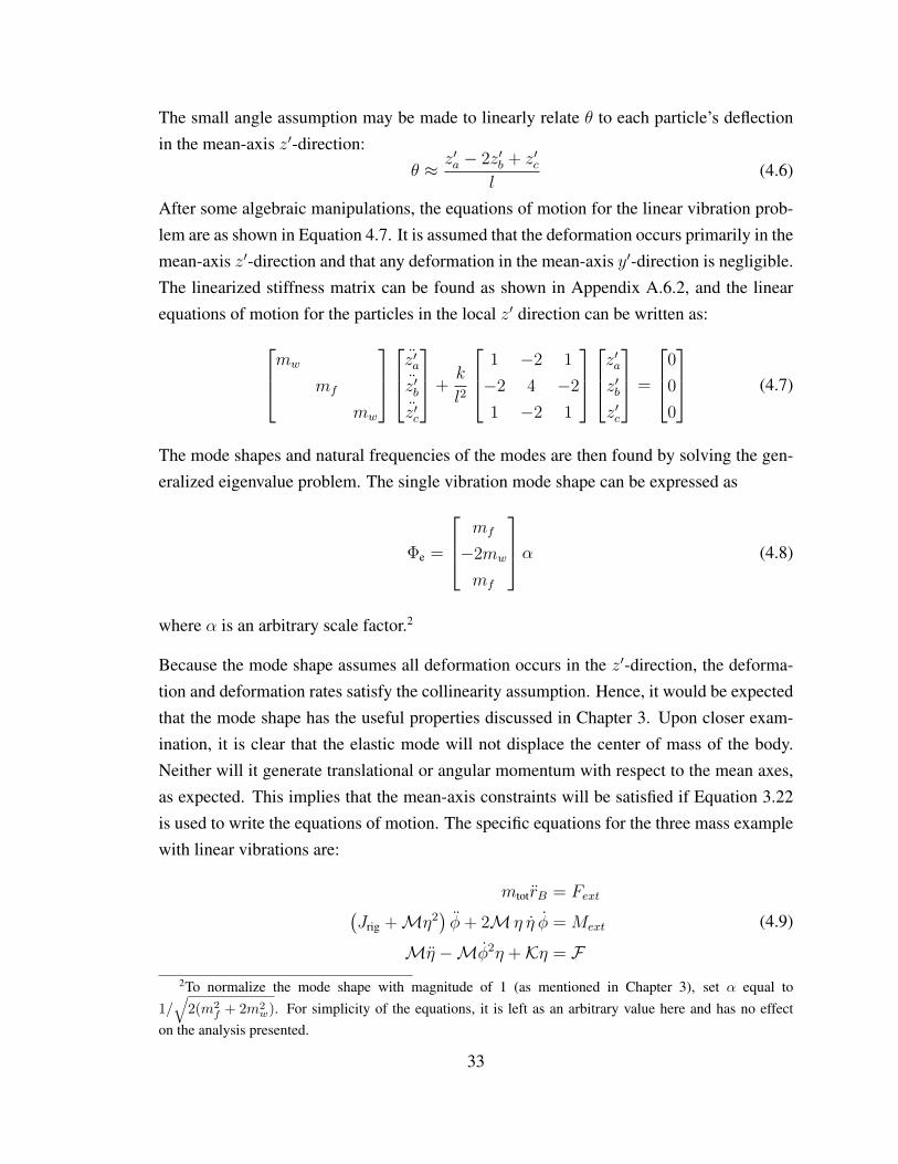
Because the mode shape assumes all deformation occurs in the z′-direction, the deforma-tion and deformation rates satisfy the collinearity assumption. Hence, it would be expectedthat the mode shape has the useful properties discussed in Chapter 3. Upon closer exam-ination, it is clear that the elastic mode will not displace the center of mass of the body.Neither will it generate translational or angular momentum with respect to the mean axes,as expected. This implies that the mean-axis constraints will be satisfied if Equation 3.22is used to write the equations of motion. The specific equations for the three mass examplewith linear vibrations are:

mtotrB = Fext(Jrig +Mη2

)φ+ 2M η η φ = Mext

Mη −Mφ2η +Kη = F

(4.9)

2To normalize the mode shape with magnitude of 1 (as mentioned in Chapter 3), set α equal to1/√2(m2

f + 2m2w). For simplicity of the equations, it is left as an arbitrary value here and has no effect

on the analysis presented.

33

whereM = 2mwmf (2mw +mf )α2 and K = 4k(2mw +mf )

2α2/l2. In comparison to thegeneral equations of motion in Equation 3.22, the number of equations are reduced due tothe planar motion and restricted motion of the particles in the local z′-direction only. Thevector rB is two-dimensional rather than three-dimensional, and the angular orientation isgiven by a scalar, rather than a three-dimensional vector. Furthermore, there is only oneelastic modal coordinate since Equation 4.7 yields two rigid body mode shapes and onlyone elastic mode shape. Additionally, planar motion also implies that the cross productterm ω × (Jω) is zero.

Although the equations for the three mass example are simpler than the most general case,the coupling terms of interest are preserved. From here, many similarities can be observedbetween the structure and content of the full equations with linearized vibrations (Equa-tion 4.9) and the small angle approximation of the nonlinear dynamics in Equation 4.3.Several differences may also be noted, however, which implies that the formulations are infact distinct. Specifically, in Equation 4.1, the equation for the nonlinear bending with an-gle θ has several unique terms which depend on variable combinations such as θ2θ and θ2θ.Equation 4.9, with linear deformation, does not have analagous terms for these quantities.

4.4 The Decoupled Equations

As previously mentioned, it is common to neglect the inertial coupling terms. In this case,if the terms that are second-order in η or involve products of η, η, or φ are assumed to besufficiently small, the equations simplify to:

mtotrB = Fext

Jrigφ = Mext

Mη +Kη = F

(4.10)

Equation 4.10 may also be calculated directly from the simplified general equations ofmotion (Equation 3.23). At this point, the simplified linear vibration equations of motion(Equation 4.10) may be compared to the nonlinear vibration equations of motion whichassume small deformation and small angular rates (Equation 4.4). The translational androtation equations are identical, with θ and η being the same except for some amplification.With the proper scaling of the mode shapes and modal coordinates, θ and η take on thesame values and the equations of motion are equivalent.

34

Chapter 5

Three Mass Simulation and Analysis

5.1 Simulation Setup

Through simulation, the validity of the linear solution and the simplifying assumptions areexplored. The simulation provides a time history of the states, the coupling terms, and theaerodynamic forces and moments. This allows for a detailed comparison of the nonlinearand linear results, as well as insight into how the coupling terms may affect those results.In order to provide meaningful simulations and assumption analysis, a simple aerodynamicforce model was first created. Only lift acting on the wing masses (a and c) is consideredin the model. Each wing mass has a control surface which may be deflected to generatelift. The surfaces are identical, and are assigned a lift coefficient and wing reference areaconsistent with the Mini-MUTT [14]. The model considers a constant forward velocity,and the control surfaces are trimmed accordingly. It is assumed that the lift always actsperpendicular to the wing, represented by the line connecting the fuselage mass and thewing mass in Figure 4.2. The angle of attack is a function of the wing mass velocityrelative to the wing orientation and the control deflection.

La =1

2ρ∞V

2∞Sw

2CLααa Lc =

1

2ρ∞V

2∞Sw

2CLααc (5.1)

αa = tan−1(Vw,a

V∞) + ξ0 + ξa αc = tan−1(

Vw,c

V∞) + ξ0 + ξc (5.2)

35

where

L = lift on wing masses

ρ∞ = freestream air density

V∞ = freestream air velocity

Sw = wing reference area for the entire span

CLα = coefficient of lift due to angle of attack

α = angle of attack

Vw = component of the masses’ inertial velocity perpendicular to the wing

ξ0 = trim control deflection

ξ = control deflection relative to the trim

Specific numerical values for the aerodynamics are given in Appendix A.6.3.

The control surface input is selected in order to excite both the elastic deflection and themean-axis rotation, which contribute to the neglected coupling terms and nonlinearities.The input consists of an asymmetric sinusoid superimposed on a higher frequency symmet-ric sinusoid. The asymmetric sinusoid excites the mean-axis rotation, and has a frequencyof 6 rad/s, which was selected to achieve large angular rates without exceeding reasonablebank limits. The high frequency sinusoid excites the vibration mode, and has a frequencyequal to the natural frequency of the bending mode, about 35 rad/s. Alternate control in-puts, such as symmetric and asymmetric doublets were considered. The responses to mostcontrol inputs, however, did not manage to excite both the rotational and vibration degreesof freedom enough to produce interesting results.

5.2 Trajectory Analysis

A worst-case scenario of rotation and elastic coupling is generated for the simulation re-sults. Using flight test data for the Mini-MUTT, upper bounds were estimated on the ex-pected rotation rates and deflection. The upper bound on the rotation rates was determinedto be around ±290°/s. The upper bound on the deflection corresponded to a bending an-gle of approximately ±20°. The largest coupling terms appear when the rotation rates anddeformation achieve these upper limits simultaneously. In order to generate these condi-tions, the symmetric sinusoid is assigned an amplitude of 7.7°and the asymmetric sinusoidis assigned an amplitude of 11°. A short window of the resulting control inputs is given in

36

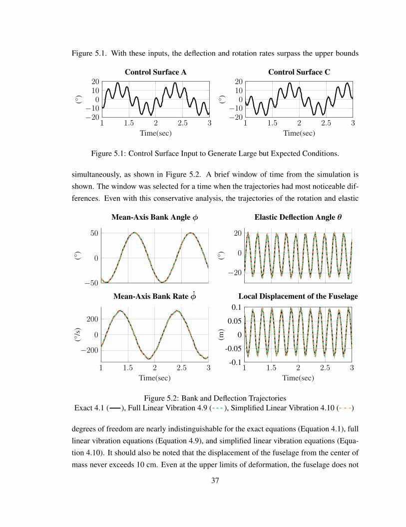
Figure 5.1. With these inputs, the deflection and rotation rates surpass the upper bounds

1 1.5 2 2.5 3−20−10

01020

Time(sec)

(°)

Control Surface A

1 1.5 2 2.5 3−20−10

01020

Time(sec)

(°)

Control Surface C

Figure 5.1: Control Surface Input to Generate Large but Expected Conditions.

simultaneously, as shown in Figure 5.2. A brief window of time from the simulation isshown. The window was selected for a time when the trajectories had most noticeable dif-ferences. Even with this conservative analysis, the trajectories of the rotation and elastic

−50

0

50

(°)

Mean-Axis Bank Angle φ

1 1.5 2 2.5 3

−200

0

200

Time(sec)

(°/s

)

Mean-Axis Bank Rate φ

−20

0

20

(°)

Elastic Deflection Angle θ

1 1.5 2 2.5 3-0.1

-0.05

0

0.05

0.1

Time(sec)

(m)

Local Displacement of the Fuselage

Figure 5.2: Bank and Deflection TrajectoriesExact 4.1 ( ), Full Linear Vibration 4.9 ( ), Simplified Linear Vibration 4.10 ( )

degrees of freedom are nearly indistinguishable for the exact equations (Equation 4.1), fulllinear vibration equations (Equation 4.9), and simplified linear vibration equations (Equa-tion 4.10). It should also be noted that the displacement of the fuselage from the center ofmass never exceeds 10 cm. Even at the upper limits of deformation, the fuselage does not

37

deform significantly relative to the mean-axis frame. Before drawing a conclusion about theeffects of the coupling terms, the trajectory of the center of mass is presented in Figure 5.3.Upon an examination of the center of mass location, differences are more noticeable. The Y

−0.6

−0.4

−0.2

0

Time (sec)

(m)

Y Position of Center of Mass rB,y

1 1.5 2 2.5 30.2

0.4

0.6

0.8

1

1.2

Time(sec)

(m)

Z Position of Center of Mass rB,z

Figure 5.3: Center of Mass TrajectoryExact 4.1 ( ), Full Linear Vibration 4.9 ( ), Simplified Linear Vibration 4.10 ( )

component of the center of mass position has the most noticeable discrepancy, but it is stillvery small. Furthermore, the linear vibration solution with and without the coupling terms,Equations 4.9 and 4.10 respectively, appear identical. This would suggest that linearizingthe vibrations has a small yet noticeable effect, but dropping the coupling terms producesnegligible differences. As compared to the exact equations of motion (Equation 4.1), theroot mean square of the error for selected quantities was averaged over the given time win-dow for the full linear vibration solution (Equation 4.9) and the linear vibration solutionwithout the coupling terms (Equation 4.10). The results are given in Table 5.1 .

Quantity Full Linear Solution 4.9 Simplified Linear Solution 4.10

φ RMS Error 0.40° 0.38°φ RMS Error 3.42°/s 2.31°/sθ RMS Error 0.37° 0.53°rB,y RMS Error 3.73 cm 3.91 cmrB,z RMS Error 1.26 cm 1.36 cm

Table 5.1: RMS Error for Three Mass Example Solutions

38

5.3 Coupling and Forcing Analysis

In order to understand why the solutions have such similar trajectories under the worst-caseconditions simulated, the coupling terms are compared to other terms of interest. In orderto clarify the analysis of the coupling terms, the equations of motion for the three massexample are rewritten (originally Equation 4.9) as:

mtotrB = Fext

(Jrig + ∆J) φ+ Ω1 = Mext

Mη + Ω2 +Kη = F

(5.3)

where ∆J = Mη2, Ω1 = 2M η η φ, and Ω2 = −Mφ2η. The coupling terms Ω1 andΩ2 are compared to the aerodynamic forces and moments. Additionally, the inertia tensorchange ∆J is compared to the rigid body inertia tensor. Finally, because the coupling termΩ2 is linear in η, it suugests that it may be viewed as a stiffening/softening term. Hence,Ω2/η may be compared to the generalized stiffness K. Because the ratios of these termsspan such large values, they are displayed on a logarithmic plot. Figure 5.4 provides vali-dation for the reasoning behind the simplifying assumptions. The aerodynamic forces andmoments are almost always much larger than the apparent forces and moments from thecoupling terms. Although the coupling terms do become comparable with the aerodynam-ics at several times, these instances are brief and their effects appear to be negligible basedon Figures 5.2 and 5.3. Additionally, the ratios of Ω2/η to K and ∆J to Jrig appear quitesmall. To more explicitly quantify these ratios, the terms are averaged over the given timewindow and then the ratio of the averages is calculated. This calculation is presented inTable 5.2.

Ω1 / Aero Moment 0.070Ω2 / Aero Modal Force 0.058

Ω2 / Stiffness Force 0.010∆J / Jrig 0.010

Ω2

η/ K 0.010

Table 5.2: Numerical Comparison of Neglected Terms to Forcing Terms

39

10−3

100

103

(Nm

)

Moments

Aero Ω1

10−4

100

104

(N)

Modal Forces

Aero Stiffness Ω2

1 1.5 2 2.5 310−5

10−2

101

Time(sec)

(kg

m2)

Inertia Tensor

Jrig ∆J

1 1.5 2 2.5 310−4

100

104

Time(sec)(N

/m)

Generalized Stiffness

Kgen Ω2/η

Figure 5.4: Coupling Term Comparison

5.4 Insight from the Three Mass Example

The simplicity of the three mass example allows for insight into a concept that can bechallenging in general. One important point that the three mass example highlights is thatthe mean axes do not only apply to a body with linear vibration modes. The conceptof the mean axes is very general, and its dynamics can be identified using equations 2.15and 2.29, even if the body is deforming in some nonlinear manner. In general, the challengeis explicitly identifying the mean axes, visualizing it, and describing the elastic motion ofthe body with respect to the mean axes. A special property of the three mass example isthat the mean axes can be explicitly identified and the elastic motion described without theuse of linear vibration modes. The mean axes can be visualized as in figure 4.2 and thedynamics can be fully specified according to equation 4.1. A similar example of a bodywith nonlinear deformation that can be described using the mean axes is presented in [7].

Because the mean axes may be explicitly identified for the nonlinear elastic deformation ofthe three mass example, it offers an opportunity to compare the effects of linearizing the

40

elastic deformation in this framework. In the context of the Mini-MUTT, the simulation re-sults showed little difference between the nonlinear and linear deformation models. For anapplication with larger expected deflection, however, this type of example may be modifiedto approximate the deflection ranges for which the linear deformation model is sufficientlyaccurate.

Furthermore, this example is sufficiently simple to examine the coupling effects commonlyneglected in the mean-axis approach. These assumptions are more difficult to validate forthe full model created with finite element mode shapes and more complex aerodynamics.When the example is tailored to represent the more complicated system, it can offer somevalidation of the assumptions that the inertia tensor is constant and that the coupling termsare negligible.

41

Chapter 6

Conclusions and Future Work

A Newtonian derivation of the mean-axis equations of motion has been presented. Theseequations are consistent with the equations produced from Lagrangian derivations, but mayoffer new insight into the formulation of the mean-axis dynamics. The additional degreesof freedom resulting from the mean-axis frame were handled precisely, and simplifyingassumptions with regard to the inertia tensor and additional coupling between rotation anddeformation were discussed. Finally, an illustrative example of a highly simplified aircraftwith lumped-mass and rolling motion was presented, and the assumptions were analyzedin the framework of this simple example. A time history of the simulated vehicle dynamicsrevealed that the solutions vary only slightly under conditions with aggressive maneuveringand large deformation. The simulation also allowed for a comparison of the coupling termsto the aerodynamic moments and generalized modal forcing. It was shown that it is reason-able to neglect the coupling terms for this example, even during extreme maneuvers anddeflection. Furthermore, it was shown that use of the linearized vibration modes providesvery close results to the equations of motion constructed with nonlinear deformation.

Some of the key assumptions made throughout this derivation of the mean-axis equations ofmotion are collinearity and a zero net internal moment of system. When these assumptionsare invalid, several unanswered questions remain. Particularly, how should a non-zerointernal moment be dealt with? Should it be ignored as a modeling or linearization error,or should it be incorporated into the flight dynamics model. In this case, what are theeffects on conservation of angular momentum and conservation of energy? A model withdeformation in multiple dimensions and more than one elastic mode shape will be requiredto investigate these effects. It may also be hypothesized that any of these errors are only

42

significant if the model is being used outside of the range of validty for linearization, inwhich case these effects may be ignored. Future work in this area will require additionalinsight into structural modeling and the effects of linearization. Ultimately, this topic mayprovide more information on when it is valid to use the mean-axis modeling technique.

43

Bibliography

[1] Milne, R. D., “Dynamics of the Deformable Aeroplane,” Aeronautical Research

Council Reports and Memoranda, , No. 3345, 1964.

[2] Buttrill, C. S., Zeiler, T. A., and Arbuckle, P. D., “Nonlinear Simulation fo a FlexibleAircraft in Maneuvering Flight,” Flight Simulation Technologies Conference, Guid-

ance, Navigation, and Control and Co-located Conferences, 1987.

[3] Schmidt, D. K., Zhao, W., and Kapania, R. K., “Flight-Dynamics and Flutter Mod-eling and Analysis of a Flexible Flying-Wing Drone,” AIAA Atmospheric Flight Me-

chanics Conference, AIAA SciTech Forum, 2016.

[4] Theis, J., Pfifer, H., and Seiler, P., “Robust Control Design for Active Flutter Supres-sion,” AIAA Atmospheric Flight Mechanics Conference, AIAA SciTech Forum, 2016.

[5] H.Pfifer, B. D., “System Identification of a Small Flexible Aircraft,” AIAA Atmo-

spheric Flight Mechanics Conference, AIAA SciTech Forum, 2016.

[6] Greenwood, D. T., Principles of Dynamics, Prentice-Hall, 1988.

[7] Canavin, J. and Likins, P., “Floating Reference Frames for Flexible Spacecraft,” Jour-

nal of Spacecraft, Vol. 14, No. 12, 1977, pp. 724–732.

[8] Waszak, M. R. and Schmidt, D. K., “Flight Dynamics of Aeroelastic Vehicles,” Jour-

nal of Aircraft, Vol. 25, No. 6, 1988, pp. 563–571.

[9] Schmidt, D. K., Modern Flight Dynamics, McGraw-Hill, 2012, ISBN9780073398112.

[10] Meirovitch, L., Elements of Vibration Analysis, McGraw-Hill, 1986.

44

[11] Agrawal, O. and Shabana, A., “Application of Deformable-Body Mean Axis to Flex-ible Multibody System Dynamics,” Computer Methods in Applied Mechanics and

Engineering, Vol. 56, 1986, pp. 217–245.

[12] Neto, A. B. G., Silva, R. G. A., Paglione, P., and Silvestre, F. J., “Formulation ofthe Flight Dynamics of Flexible Aircraft Using General Body Axes,” AIAA Journal,Vol. 54, No. 11, 2016, pp. 3516–3534.

[13] Meirovitch, L., “Hybrid State Equations of Motion for Flexible Bodies in Terms ofQuasi-Coordinates,” Journal of Guidance, Control, and Dynamics, Vol. 14, No. 5,1991, pp. 1008–1013.

[14] Regan, C. D. and Taylor, B. R., “mAEWing1: Design, Build, Test,” AIAA Atmo-

spheric Flight Mechanics Conference, AIAA SciTechForum, 2016.

45

Appendix A

Appendices

A.1 Useful Facts of Modal Matrices

Some useful facts regarding properties of the modal matrix are presented here for usethroughout the Appendix.

1. ΦTTMΦT = mtotI3:

Recall that M = diag(m1I3, . . . ,mnI3) and ΦT := [I3, . . . , I3]T by definition of thetranslational mode shapes (Equation 3.3). Hence ΦT

TMΦT =∑n

i=1 miI3 := mtotI3.

2. ΦTTMΦ(s)η = mtotηT :

It follows from modal orthogonality that ΦTTMΦ(s)η = ΦT

TMΦTηT (only the termscorresponding to the translational coordinates ηT remain). By Fact 1, ΦT

TMΦTηT =

mtotηT . This is also true for derivatives of ηT . Hence, ΦTTMΦ(s)η = mtotηT and

ΦTTMΦ(s)η = mtotηT .

3. ΦTTMb = 0 and ΦT

TMs = 0:Note that ΦT

TMb =∑n

i=1 mibi. This term is zero because the center of mass isassumed to be at the origin for all possible deformations. Equivalently stated, themean-axis translational constraint (Definition A.2.A) implies that

∑ni=1 mibi = 0 by

Theorem 1. Similarly, ΦTTMs =

∑ni=1misi. This term is zero because the center

of mass is assumed to be at the origin when the particles are in their undeformedpositions.

46

4. s+ Φ(s)η = s+ δ = b:The deformation δ is described using a modal matrix computed with the undeformedshapes, Φ(s). Therefore, δ = Φ(s)η. Recall that s+ δ = b and hence s+ Φ(s)η = b.

5. ΦR(b) = ΦR(s) + ΦR(δ):Recall that ΦR(b)T := [b×1 , . . . , b

×n ]T by definition of the rotational mode shapes

(Equation 3.5). Moreover, bi = si + δi and [b×1 , . . . , b×n ]T = [(s1 + δ1)×1 , . . . , (sn +

δn)×]T = [s×1 , . . . , s×n ]T + [δ×1 , . . . , δ

×n ]T . Hence ΦR(b) = ΦR(s) + ΦR(δ).

6. Jω =∑n

i=1 mibi × (ω × bi) = ΦR(b)TMΦR(b)ω

J =∑n

i=1mi(bTi biI3 − bibTi ) = ΦR(b)TMΦR(b):

Recall that the inertia tensor can be written in several ways. Let [xi, yi, zi]T be the

components of the vector bi expressed in the body frame. The inertia tensor is definedas

J =

Jxx Jxy Jxz

Jyx Jyy Jyz

Jzx Jzy Jzz

(A.1)

where Jxx =∑n

i=1mi(y2i + z2

i ), Jxy = −∑n

i=1mi(xiyi), etc. This can be writtenmore concretely as J =

∑ni=1 mi(b

Ti biI3 − bibTi ).

The inertia tensor J can be multiplied by the angular velocity ω to write Jω =∑ni=1mi (|bi|2ω − (bi · ω)bi). It follows from the vector triple product identity that

this can equivalently written as Jω =∑n

i=1 mibi × (ω × bi). Finally, this term canbe written in matrix form. Using the cross product property that (a× b) = −(b× a),it can be seen that

∑ni=1 mibi × (ω × bi) = −

∑ni=1mibi × (bi × ω). This form for

Jω can be written using the modal matrices as follows:

Jω = [−b×1 , . . . ,−b×n ]

m1I3

. . .

mnI3

[b×1 ω, . . . , b×nω] (A.2)

Thus it follows from Fact 5 that Jω = ΦR(b)TMΦR(b)ω. From the form of thisterm, it can be concluded that an additional form for the inertia tensor is J =

ΦR(b)TMΦR(b).

Similarly, Jω =∑n

i=1 mi (|bi|2ω − (bi · ω)bi) =∑n

i=1 mibi × (ω × bi).

47

7. Jrig = ΦR(s)TMΦR(s):From the matrix form of J given in the explanation of Fact 6, it can be concludedthat substituting s for b in J = ΦR(b)TMΦR(b) will yield Jrig = ΦR(s)TMΦR(s),where Jrig is the rigid body (or undeformed) inertia tensor.

8. JrigηR = ΦR(s)TMΦ(s)η =∑n

i=1misi × δi =∑n

i=1misi × δR,i:Written in summation form, ΦR(s)TMΦ(s)η =

∑ni=1misi × δi. It follows from

modal orthogonality that ΦR(s)TMΦ(s)η = ΦR(s)TMΦR(s)ηR. By Fact 7, thisterm is JrigηR. Similarly, ΦR(s)TMΦ(s)η = JrigηR.

Additionally,∑n

i=1misi × δR,i = ΦTR(s)MΦR(s)ηR. By Fact 7, this can be recog-

nized as JrigηR.

9. Jω =∑n

i=1 mibi × (ω × δi) +∑n

i=1 miδi × (ω × bi):From Fact 6, the inertia tensor J can be written as J = ΦR(b)TMΦR(b). Takingthe derivative of this expression results in J = ΦR(b)TMΦR(δ) + ΦR(δ)TMΦR(b).By the explanation for Fact 6, it can be seen that Jω =

∑ni=1mibi × (ω × δi) +∑n

i=1miδi × (ω × bi).

A.2 Simplification of Translational Dynamics in Mean Axes

The body-referenced equations associated with multiplication by ΦTT are given Equation 3.10a

and repeated below:

ΦTT (Ma+KΦ(s)η) = ΦT

TF (3.10a)

where a is given by:

a := ΦT rB + Φ(s)η + Ω×(s+ Φ(s)η) + Ω×Ω×(s+ Φ(s)η) + 2Ω×Φ(s)η (A.3)

The various terms in this ODE can be simplified as follows:

1. ΦTTMΦT rB = mtotrB: This is true by Fact 1.

2. ΦTTMΦ(s)η = mtotηT : This is true by Fact 2.

3. ΦTTMΩ×(s + Φ(s)η) = mtotω

×ηT : Recall that Ω× := diag(ω×, . . . , ω×). ThusΦTTMΩ× can be equivalently written as ω×ΦT

TM . Next, ΦTTMs = 0 by Fact 3.

48

Moreover, ΦTTMΦ(s)η = mtotηT by Fact 2. Combining these facts yields the desired

simplification for this term.

4. ΦTTMΩ×Ω×(s + Φ(s)η) = mtotω

×ω×ηT : Similar to the simplification of Term 3,this term can be rewritten and simplified usings Facts 2 and 3.

5. 2ΦTTMΩ×Φ(s)η = 2mtotω

×ηT : This involves similar steps to those given for thesimplification of Term 3, using Facts 2 and 3.

6. ΦTTKΦ(s)η = 0: This term first simplifies to ΦT

TKΦTηT by the modal orthogonality(similar to Fact 2). Then use the fact that rigid body translations yield no restoringforce to conclude that KΦT = 0 and this term must be zero.

7. ΦTTF =

∑ni=1 Fi := Fext: This follows from the structure of ΦT = [I3, . . . , I3]T .

Combining these simplifications finally yields the following form for the translational dy-namics:

mtot

(rB + ηT + ω×ηT + ω×ω×ηT + 2ω×ηT

)= Fext (A.4)

A.3 Simplification of Rotational Dynamics in Mean Axes

The body-referenced equations associated with multiplication by ΦR(b)T are given Equa-tion 3.10b and repeated below:

ΦR(b)T (Ma+KΦ(s)η) = ΦR(b)TF (3.10b)

where a is again given by:

a := ΦT rB + Φ(s)η + Ω×(s+ Φ(s)η) + Ω×Ω×(s+ Φ(s)η) + 2Ω×Φ(s)η (A.5)

The various terms in this ODE can be simplified as follows:

1. ΦR(b)TMΦT rB = 0: Recall that M = diag(m1I3, . . . ,mnI3) and ΦR(b)T :=

[b×1 , . . . , b×n ]T by definition of the rotational mode shapes (Equation 3.5). Hence

ΦR(b)TMΦT rB =∑n

i=1 mibi × rB. This can be rewritten as −rB ×∑n

i=1mibi,which is zero by Fact 3.

49

2. ΦR(b)TMΦ(s)η = JrigηR+∑n

i=1 miδi× δi: By Fact 5, this term may be rewritten asΦR(s)TMΦ(s)η + ΦR(δ)TMΦ(s)η. By Fact 8, ΦR(s)TMΦ(s)η = JrigηR. Finally,ΦR(δ)TMΦ(s)η can be rewritten as

∑ni=1miδi × δi.

3. ΦR(b)TMΩ×(s+Φ(s)η) = Jω: By Fact 4, this term can be written as ΦR(b)TMΩ×b.By the form of Ω×, this can be written as

∑ni=1mibi × (ω× bi). By Fact 6, this term

is equal to Jω.

4. ΦR(b)TMΩ×Ω×(s + Φ(s)η) = ω × (Jω): This term can be written as the summa-tion

∑ni=1 mibi × (ω × (ω × bi)), which can be rewritten using the Jacobi identity1

to yield∑n

i=1 mi [(ω × bi)× (ω × bi) + ω × (bi × (ω × bi))]. The first term in thesummation is zero since a vector cross product with itself is zero. The expressionmay now be rewritten as ω ×

∑ni=1mi (bi × (ω × bi)) which, by Fact 6, is known to

be ω × (Jω).

5. 2ΦR(b)TMΩ×Φ(s)η = Jω+ω× (JrigηR) +ω×∑n

i=1mi

(δi × δi

): This term can

be written in summation form to show that 2ΦR(b)TMΩ×Φ(s)η = 2∑n

i=1mibi ×(ω × δi). This term can be split into two identical terms, and then one of the termsmay be rewritten using the Jacobi Identity (defined previously) to yield

∑ni=1mibi×

(ω × δi) +∑n

i=1mibi × (ω × δi) =∑n

i=1 mibi × (ω × δi) +∑n

i=1 miδi × (ω ×bi) + ω ×

∑ni=1mi(bi × δi). Substituting si + δi for bi in the last additive term, this

expression can be written as∑n

i=1 mibi × (ω × δi) +∑n

i=1 miδi × (ω × bi) + ω ×∑ni=1mi(si × δi) + ω ×

∑ni=1 mi(δi × δi). By Facts 8 and 9, this expression can be

further rewritten as Jω + ω × JrigηR + ω ×∑n

i=1mi(δi × δi).

6. ΦR(b)TKΦ(s)η = 0: This term represents the moment due to internal forces in thebody. This term can be separated into two terms as ΦR(s)TKΦ(s)η+ΦR(δ)TKΦ(s)η.The first term simplifies to ΦR(s)TKΦR(s)ηR by modal orthogonality. Becausethe rigid body rotation yields no restoring force, KΦR = 0 and this term mustbe zero. Note that the second term may be written as

∑ni=1

(δi ×

∑nj=1Kijδj

)=∑n

i=1

∑nj=1Kij (δi × δj). If the collinearity assumption is satisfied, this expression

becomes∑n

i=1

∑nj 6=iKij (δi × δj). Moreover, because Kij = Kji and (δi × δj) =

− (δj × δi), this expression simplifies to zero and hence ΦR(b)TKΦ(s)η = 0.

Regardless of collinearity, it can be noted that the internal moment Mint should bezero according to first principles. As discussed prior to the presentation of Equa-tion 2.1, the internal force on particle i due to particle j is denoted by F ij . By

1The Jacobi identity states that a× (b× c) = c× (b× a) + b× (a× c).

50

Newton’s Third Law, the internal forces between particles i and j are assumed tobe equal and opposite: F ij = −F ji. Moreover, the internal forces are assumed toact along the line between the two particles: F ij = |F ij|(rj − ri). Because theforces have equal magnitude and opposite direction, as well as collinearity, the mo-ment created by F ij will be exactly opposite to that created by F ji. Therefore, ifthe model is reasonably accurate and captures this fundamental property that followsfrom Newton’s Third Law, the net internal moment Mint will be zero.

Conversely, if the model results in a non-zero net internal moment, i.e. Mint 6= 0,then conservation of angular momentum will be violated. A non-zero internal mo-ment will result in a non-zero rate of change of angular momentum, even if no mo-ment is generated by outside forces. Hence the system will not satisfy conservationof angular momentum.

In reality, however, if collinearity is not satisfied then a non-zero internal momentmay exist due to modeling errors. For completeness, therefore, a non-zero net in-ternal moment may be considered in the form of ΦR(δ)TKΦ(s)η = −Mint. If theinternal moment is retained, it must be added to the forcing of the mean-axis rota-tional dynamics in Equation 2.29.

7. ΦR(b)TF =∑n

i=1Mi := Mext: This follows from the structure of ΦR(b)T :=[b×1 , . . . , b

×n

]. Note that Mext is the total moment due to external forces and does

not account for any net internal moment. Hence ΦR(b)TF =∑

i bi × Fi and thisterm is equal to Mext :=

∑iMi as claimed.

A.4 Internal Angular Momentum and its Derivative in Mean Axes

In component form, the internal angular momentum in the mean-axis reference frame is:

Hint =n∑i=1

mibi × δi (A.6)

Using Fact 4 and 8, the expression for internal angular momentum in the mean axes be-comes:

Hint = JrigηR +n∑i=1

miδi × δi (A.7)

51

Applying the transport theorem, the rate of change of the internal angular momentum is:

Hint = JrigηR + ω × (JrigηR) +n∑i=1

δi ×miδi + ω ×n∑i=1

(δi ×miδi

)(A.8)

A.5 Simplification of Elastic Dynamics in Mean Axes

The body-referenced equations associated with multiplication by ΦTE are given Equation 3.10c

and repeated below:

ΦTE (Ma+KΦ(s)η) = ΦT

EF (3.10c)

where a is again given by:

a := ΦT rB + Φ(s)η + Ω×(s+ Φ(s)η) + Ω×Ω×(s+ Φ(s)η) + 2Ω×Φ(s)η (A.9)

Before simplifying the terms of the elastic dynamics, a useful property that follows fromcollinearity of elastic deformation will be derived. Recall that collinearity implies∑n

i=1miδE,i × δE,i = 0. To proceed the following new notation is needed:

δ×E(ηE) =

−δ×E,1

...−δ×E,n

(A.10)

where the superscript × indicates the skew symmetric matrix corresponding to the crossproduct. (ηE) is included here to emphasize that δ×E is a function of the elastic modalcoordinates, but it will subsequently be dropped. Now the collinearity expression can berewritten in modal form as δ×TE (ηE)MΦE ηE = 0. This equality must hold for all possiblesolutions ηE(t) and ηE(t). In particular, it must hold for all possible initial conditionsηE(0) and ηE(0). These initial conditions can be specified independently and hence it mustbe true that:

δ×TE MΦE = 0 (A.11)

It can similarly be shown thatδ×TE MΦE = 0 (A.12)

The various terms in the ODE 3.10c can now be simplified as follows:

52

1. ΦTEMΦT rB = 0: Recall that the mode shapes are orthogonal through the mass ma-

trix. By definition, this means that ΦTEMΦT = 0.

2. ΦTEMΦ(s)η = ME ηE: Modal orthogonality through the mass matrix implies that

ΦTEMΦ(s)η = ΦT

EMΦE ηE . Moreover, ΦTEMΦE :=ME whereME is the general-

ized mass matrix associated with the elastic modal coordinates.

3. ΦTEMΩ×(s+ Φ(s)η) = 0: This expression can be rewritten as ΦT

EMΩ×s+

ΦTEMΩ×Φ(s)η. Due to the form of Ω×, the first term can be written as

ΦTEM

[s×1 . . . s

×n

]Tω = ΦT

EMΦR(s)ω. From modal orthogonality, ΦTEMΦR(s) = 0,

and hence the first time is eliminated. The second term is simplified if collinearity isassumed and ηR = 0 (which requires the additional assumption that Mint = 0 as de-scribed in Theorem 4). Under the assumption that ηR = 0, the second term becomesΦTEMΩ×ΦEηE . This can be written as ΦT

EMδ×E ω. It follows from equation A.11 thatΦTEMδ×E ω = δ×TE MΦE = 0, and hence the second term is also eliminated.

4. ΦTEMΩ×Ω×(s + Φ(s)η) = ΦT

EMΩ×Ω×(s + ΦEηE): This term simplifies slightlyunder the assumption that ηR = 0. Φ(s)η becomes ΦEηE .

5. 2ΦTEMΩ×Φ(s)η = 0: Under the assumption that ηR = 0, the expression becomes

2ΦTEMΩ×ΦE ηE . Due to the form of Ω×, the expression can be written as 2ΦT

EMδ×Eω.From equation A.12, ΦT

EMδ×E = 0 and the term is eliminated.

6. ΦTEKΦ(s)η = KEηE: This term represents the restoring modal forces due to the

stiffness in the body. Due to modal orthogonality, ΦTEKΦ(s)η = ΦT

EKΦEηE . More-over, ΦT

EKΦE := KE where KE is the generalized stiffness matrix associated withthe elastic modal coordinates.

7. ΦTEF := FE: This term is defined as the elastic modal forcing FE .

A.6 Three Mass Example Supplementary Material

A.6.1 Numerical Values for the Three Mass Structure

Specific numerical values for the structure that makes up the simplified aircraft in the threemass example are:

53

mf 5 kgmw 2 kgl 1 mk 692.9 Nm/rad

Table A.1: Numerical Values for the Three Mass Structure

A.6.2 Linearized Stiffness

In order to use linear equations to describe the deformation of the three mass example,the stiffness matrix must be calculated. The textbook technique involves taking partialderivatives of the elastic potential energy with respect to the motion of each particle, butan alternate approach is given here. Recall from Equation 4.6 that θ ≈ z′a−2z′b+z

′c

l. This

equation can be used to write theta in matrix form as:

θ ≈ 1

l

[1 −2 1

]z′ (A.13)

where z′ =[z′a z′b z′c

]T. Note also that the potential energy due to deformation may be

written as:V = θTkθ ≈ (z′)TKz′ (A.14)

where V is the potential energy, k is the bending stiffness, and K is the linearized stiff-ness matrix. Note that θ is unaffected by the transpose since it is a scalar. SubstitutingEquation A.13 for θ in Equation A.14, it can be shown that:

(z′)Tk

l2

1

−2

1

[1 −2 1]z′ = (z′)TKz′ (A.15)

From this equation, it can be concluded that:

K =k

l2

1

−2

1

[1 −2 1]

=k

l2

1 −2 1

−2 4 −2

1 −2 1

(A.16)

54

A.6.3 Numerical Values for the Three Mass Aerodynamics

Specific numerical values for the structure that makes up the simplified aircraft in the threemass example are:

ρ∞ 1.2266 kg/m2

V∞ 27.432 m/sSW 1.068 m2

CLα 4.5

ξ02g(2mw+mf)ρ∞V 2

∞SWCLα

Table A.2: Numerical Values for the Three Mass Aerodynamics

55