Rowan University Rowan University

Rowan Digital Works Rowan Digital Works

Theses and Dissertations

1-14-2014

A new software tool to environmentally and economically A new software tool to environmentally and economically

evaluate solvent recovery in the pharmaceutical industry evaluate solvent recovery in the pharmaceutical industry

Eduardo Cavanagh

Follow this and additional works at: https://rdw.rowan.edu/etd

Part of the Chemical Engineering Commons

Recommended Citation Recommended Citation Cavanagh, Eduardo, "A new software tool to environmentally and economically evaluate solvent recovery in the pharmaceutical industry" (2014). Theses and Dissertations. 295. https://rdw.rowan.edu/etd/295

This Thesis is brought to you for free and open access by Rowan Digital Works. It has been accepted for inclusion in Theses and Dissertations by an authorized administrator of Rowan Digital Works. For more information, please contact graduateresearch@rowan.edu.

A NEW SOFTWARE TOOL TO ENVIRONMENTALLY AND

ECONOMICALLY EVALUATE SOLVENT RECOVERY IN THE

PHARMACEUTICAL INDUSTRY

by

Eduardo Juan Cavanagh

A Thesis

Submitted to the

Department of Chemical Engineering

College of Engineering

In partial fulfillment of the requirement

For the degree of

Master of Science in Engineering

at

Rowan University

November, 14, 2013

Thesis Chairs: Mariano Savelski, Ph.D., C. Stewart Slater, Ph.D

© 2013 Eduardo Juan Cavanagh

Dedication

To my family Eduardo Cavanagh, Elena Martinez Vivot, Glubi Cavanah, Lola Cavanagh

and Helena Cavanagh. To Esther Cornejo Butler. To Lucas Mendos, Nicolás Ferretti,

Juan Pablo Kunz, Ignacio Espinosa, Diego Filpo, Patricio Barciela, Juan Simonelli,

Carolina Olascoaga, Diego Rhode, Paula Bruni, Mariela Pistasoli, Silvina Fernandez

Vidal, Alejandro Corizzo, Maria Schoendfel and Francisco Ferretti.

iv

Acknowledgments

To my advisors Dr. Mariano Savelski and Dr. C. Stewart Slater. To Frank

Urbanski and Carlos Junco from Pfizer, Inc. To Leland Vane and Nora Lopez from U.S.

EPA. To Harold Wandke from Sulzer. To former and current Rowan University students

Mike Raymond, Dave Hitchcock, Molly Russell, Stephen Montgomery, Mihika Padia,

Matt Bucchanan and Bill Hoffman.

v

Abstract

Eduardo Juan Cavanagh

A NEW SOFTWARE TOOL TO ENVIRONMENTALLY AND ECONOMICALLY

EVALUATE SOLVENT RECOVERY IN THE PHARMACEUTICAL INDUSTRY

2012/13

Mariano Savelski, Ph.D., C. Stewart Slater, Ph.D.

Master of Science in Chemical Engineering

The environmental impact reduction and operating costs savings associated with

the purification and recuse of solvent waste in the manufacture of active pharmaceutical

ingredients (API’s) were investigated. A software toolbox has been developed that

combines Aspen Plus® process simulation with SimaPro® and Ecosolvent life cycle

assessment (LCA) databases. The feasibility of a relatively small flexible skid capable of

recovering multiple solvent waste streams was evaluated. Fractional distillation and

pervaporation were considered to separate binary solvent waste mixtures. Optimum

distillation reflux ratio and feed stage were determined to maximize the environmental

impact reductions and operating cost savings. The optimum reflux ratio was significantly

higher than suggested by traditional heuristics. The emissions and cost reductions

obtained were as much as 43 % and 59 % higher, respectively, as compared to using the

conventional optimum reflux ratio. A comprehensive cash flow analysis showed that the

recovery of low volume solvent waste streams can be economically feasible, despite

traditional thinking. It has been demonstrated that the flexibility of a skid to recover

solvent waste streams of different thermodynamic nature and volume is a key issue to

increase profitability. Four case studies from Pfizer are presented to show how our

software tool can aid in green engineering decision making.

vi

Table of Contents

Abstract ............................................................................................................................... v

List of Figures .................................................................................................................... ix

List of Tables ................................................................................................................... xiii

Chapter 1: Introduction ....................................................................................................... 1

Life Cycle Assessment of Organic Solvents Recovery in the Pharmaceutical Industry 9

Life Cycle Emissions Avoided in Solvent Recovery. ............................................... 12

Solvent Recovery Economics. .................................................................................. 15

Solvent Recovery Barriers ............................................................................................ 17

Recovery Technologies Analysis .................................................................................. 18

Fractional Distillation ............................................................................................... 18

Fractional Crystallization .......................................................................................... 19

Extraction .................................................................................................................. 20

Extractive Distillation (or Azeotropic Homogeneous Distillation) .......................... 21

Pervaporation ............................................................................................................ 22

Chapter 2: Solvent Recovery Assessment Software Toolbox: R.SWEET ....................... 25

Recovery Process Selection Guide ............................................................................... 28

Process Simulation ........................................................................................................ 30

How it Works ............................................................................................................ 30

How to Use it ............................................................................................................ 38

Cash Flow Analysis ...................................................................................................... 41

Comparison with Other Tools ....................................................................................... 42

Chapter 3: Case Studies .................................................................................................... 44

The Skid ........................................................................................................................ 45

Skid Economics ........................................................................................................ 47

General Considerations ................................................................................................. 48

Selamectin Case: Acetone and Acetonitrile .................................................................. 49

Overview ................................................................................................................... 49

Thermodynamic Evaluation and Recovery Process Design ..................................... 53

Life Cycle Assessment .............................................................................................. 55

vii

Nelfinavir Case: IPA and THF ..................................................................................... 56

Overview ................................................................................................................... 56

Thermodynamic Evaluation and IPA Recovery Process Design .............................. 58

Life Cycle Assessment .............................................................................................. 60

Hydrocortisone Case: Toluene and Acetone ................................................................. 61

Overview ................................................................................................................... 61

Thermodynamic Evaluation and Recovery Process Design ..................................... 63

Life Cycle Inventory ................................................................................................. 65

Celecoxib Case: IPA and Water ................................................................................... 65

Overview. .................................................................................................................. 65

Thermodynamic Analysis and Recovery Process Design ........................................ 66

Life Cycle Analysis. ................................................................................................. 68

Chapter 4: Results and Discussion .................................................................................... 70

Conventional vs. R.SWEET’s Optimum Reflux Ratio ................................................. 87

Pervaporation Membranes Comparison with R.SWEET .............................................. 92

Chapter 5: A Heterogeneous Case Study .......................................................................... 93

Chapter 6: Green Solvents ................................................................................................ 98

Chapter 7: Conclusions ................................................................................................... 114

Acknowledgments........................................................................................................... 115

List of References ........................................................................................................... 116

Appendix A: Organic Solvents available in R.SWEET .................................................. 122

Appendix B: Detailed Recovery Process Selection Guide Functioning ......................... 123

Appendix C: UNIQUAC Thermodynamic Behavior Prediction vs. Experimental Data 140

Appendix D: Pervaporation Membrane Coefficients, Standard Temperature and Energy

of Activation ................................................................................................................... 145

Appendix E: Diagram representation of pervaporation calculations .............................. 146

Appendix F: Detailed Organic Solvents LCI .................................................................. 147

Appendix G: Utilities LCI .............................................................................................. 151

Appendix H: LCA Results of Case Studies .................................................................... 156

Appendix I: Detailed Economic Results of Case Studies ............................................... 166

Appendix J: Skid Investment Cost Calculation .............................................................. 168

viii

Appendix K: Underwood Minimum Reflux Ratio Calculation ...................................... 170

Appendix L: List of Acronyms and Abbreviations......................................................... 172

ix

List of Figures

Figure Page

Figure 1. Mass of organic solvents not recovered (incinerated or released) in the

pharmaceutical industry in the United States, EPA’s TRI, 2010 Data5. Not all solvents are

included in the TRI, such as acetone or tetrahydrofuran. ................................................... 3

Figure 2. Solvent Waste Management in the United States, EPA’s TRI, 2010 Data5. ....... 4

Figure 3. Annual waste from the pharmaceutical sector in the United States, as reported

by the TRI5 ......................................................................................................................... 6

Figure 4. Illustrative process diagram of a multistep API manufacturing process and

solvent waste generation. .................................................................................................... 7

Figure 5. EPA’s Waste Management Hierarchy. Adapted from EPA’s website. ............... 8

Figure 6. Life cycle carbon footprint and cumulative energy demand of the production of

organic solvents and conventional fuels. .......................................................................... 10

Figure 7. Life cycle flow diagram of organic solvent use in the pharmaceutical industry.

........................................................................................................................................... 11

Figure 8. The impact of solvent recovery in the life cycle in the pharmaceutical industry.

........................................................................................................................................... 12

Figure 9. Integration of pervaporation with distillation for solvent recovery from

azeotropic aqueous-solvent waste system. A: Distillation Column, B: Pervaporation Unit.

........................................................................................................................................... 24

Figure 10. Differential elements (area segments) in a pervaporation membrane. R:

Retentate, P: Permeate, F: Feed, T: Retentate temperature. A: differential elements area

(A1 = A2 = A3 = … = AN = A). ......................................................................................... 35

Figure 11. IPA flux across Sulzer’s PERVAP 2201 pervaporation membrane as a

function of IPA mass fraction in the feed. Adapted from Qiao et al.. .............................. 38

Figure 12. Procedure for solvent recovery optimization .................................................. 41

Figure 13. Simple PFD for waste recovery of acetonitrile/acetone. The green square

highlights the location of the proposed recovery in the API manufacturing process. ...... 51

Figure 14. Vapor-liquid equilibrium T-x-y diagram for acetone and acetonitrile at P = 1.0

atm. Generated in Aspen Plus®

with UNIQUAC. ............................................................ 54

x

Figure 15. Vapor-liquid equilibrium x-y diagram for acetone and acetonitrile at P = 1.0

atm. Generated in Aspen Plus®

with thermodynamic property method UNIQUAC. ....... 54

Figure 16. Acetonitrile and acetone recovery scheme in the selamectin case. ................. 55

Figure 17. Vapor-liquid equilibrium T-x-y diagram for the IPA and THF at P = 1 atm,

generated in Aspen Plus®

with thermodynamic property method UNIQUAC. ............... 59

Figure 18. Vapor-liquid equilibrium x-y diagram for IPA and THF at P = 1 atm,

generated in Aspen Plus®

with thermodynamic property method UNIQUAC. ............... 59

Figure 19. IPA recovery scheme in the nelfinavir case. ................................................... 60

Figure 21. Vapor-liquid equilibrium T-x-y diagram for acetone and toluene at P = 1 atm.

........................................................................................................................................... 64

Figure 22. Vapor-liquid equilibrium x-y diagram for acetone and toluene at P = 1 atm. . 64

Figure 23. Toluene and acetone recovery scheme in the hydrocortisone case. ................ 65

Figure 24. Vapor-Liquid Equilibrium T-x-y diagram for IPA and water at P = 1 atm ..... 67

Figure 25. Vapor-Liquid Equilibrium x-y diagram for IPA and water at P = 1 atm. ........ 68

Figure 26. IPA recovery scheme in the celecoxib case. ................................................... 68

Figure 27. Sensitivity analysis of the LCEA, OCS and recovery with the reflux ratio as

the independent variable, for the acetonitrile recovery (first distillation) in the selamectin

case study. The feed stage remains constant at the optimum value of 4. ......................... 73

Figure 28. Sensitivity analysis of the LCEA, OCS and recovery with the feed stage as the

independent variable, for acetonitrile recovery (first distillation) in the selamectin case

study. The reflux ratio remains constant at the optimum value of 9. ................................ 73

Figure 29. Sensitivity analysis of the manufacture and incineration LCEA, recovery

process emissions generated, and recovery with the reflux ratio as the independent

variable, for the selamectin case study. The feed stage remains constant at the optimum

value of 4........................................................................................................................... 74

Figure 30. Sensitivity analysis of the LCEA, OCS and recovery with the reflux ratio as

the independent variable, for the acetone recovery (second distillation) in the selamectin

case study. The feed stage remains constant at the optimum value of 6. ......................... 75

Figure 31. LCEA, OCS and recovery sensitivity analysis with the feed stage as the

independent variable, for the acetone recovery (second distillation) in the selamectin case

study. The reflux ratio remains constant at the optimum value of 9. ................................ 75

xi

Figure 32. LCEA, OCS and recovery sensitivity analysis with the reflux ratio as the

independent variable, for the nelfinavir case study. The feed stage remains constant at the

optimum value of 5. .......................................................................................................... 76

Figure 33. Sensitivity analysis of the LCEA, OCS and recovery with the feed stage as the

independent variable, for the nelfinavir case study. The reflux ratio remains constant at

the optimum value of 14. .................................................................................................. 77

Figure 34. Sensitivity analysis of the LCEA, OCS and recovery with the reflux ratio as

the independent variable, for the hydrocortisone case study. The feed stage remains

constant at the optimum value of 6. .................................................................................. 78

Figure 35. LCEA, OCS and recovery sensitivity analysis with the feed stage as the

independent variable, for the hydrocortisone case study. The reflux ratio remains constant

at the optimum value of 5. ................................................................................................ 79

Figure 36. Sensitivity analysis of the LCEA, OCS and recovery with the reflux ratio as

the independent variable, for the celecoxib case study. The feed stage remains constant at

the optimum value of 6. .................................................................................................... 80

Figure 37. Sensitivity analysis of the LCEA, OCS and recovery with the feed stage as the

independent variable, for the celecoxib case study. The reflux ratio remains constant at

the optimum value of 2. .................................................................................................... 81

Figure 38. Life cycle emissions comparison between base case and recovery case in the

selamectin case study. ....................................................................................................... 82

Figure 39. Life cycle emissions comparison between base case and recovery case in the

nelfinavir case study. ........................................................................................................ 83

Figure 40. Life cycle emissions comparison between base case and recovery case in the

hydrocortisone case study. ................................................................................................ 83

Figure 41. Life cycle emissions comparison between base case and recovery case in the

celecoxib case study. ......................................................................................................... 84

Figure 42. Operating costs comparison between base case and recovery case in the

selamectin case study. ....................................................................................................... 84

Figure 43. Operating costs comparison between base case and recovery case in the

nelfinavir case study. ........................................................................................................ 85

Figure 44. Operating costs comparison between base case and recovery case in the

hydrocortisone case study. ................................................................................................ 85

Figure 45. Operating costs comparison between base case and recovery case in the

celecoxib case study. ......................................................................................................... 86

xii

Figure 46. Conventional optimum reflux ratio analysis. Adapted from Seader et al (1997).

........................................................................................................................................... 91

Figure 47. Information output of the RPSG for the hypothetical case study of MEK and

water. ................................................................................................................................. 93

Figure 48. MEK dehydration process for the heterogeneous case study. ......................... 94

Figure 49. Sensitivity analysis of the LCEA, OCS with the reflux ratio as the independent

variable, for the heterogeneous case study. The feed stage remains constant at the

optimum value of 5. .......................................................................................................... 96

Figure 50. Sensitivity analysis of the LCEA, OCS with the feed stage as the independent

variable, for the heterogeneous case study. The reflux ratio remains constant at the

optimum value of 2. .......................................................................................................... 96

Figure 51. Alternative process to dehydrate MEK and increase its recovery. D1 and D2:

distillation columns. .......................................................................................................... 97

Figure 52. MeTHF and water vapor-liquid equilibrium. An azeotrope occurs at a mole

fraction of 0.88 at atmospheric pressure. ........................................................................ 101

Figure 53. MeTHF and water T-x-y equilibrium diagram, including liquid-liquid

equilibrium. Liquid 1 is rich in water, and Liquid 2 is rich in MeTHF. ......................... 102

Figure 54. Pseudobinary diagram at 30 % entrainer to feed ratio (P = 1 atm), adapted

from Gomez et al.29

......................................................................................................... 106

Figure 55. Block flow diagram for the extractive distillation of THF from water using

glycerol as an entrainer. .................................................................................................. 107

Figure 56. Dehydration of THF integrating distillation and pervaporation. ................... 108

Figure 57. MeTHF recovery process. LS: Light Phase Stream (high concentrations of

MeTHF), HS: Heavy Phase Stream (high concentrations of water) ............................... 109

Figure 58. Total emission generated in the recovery cases ............................................ 111

xiii

List of Tables

Table Page

Table 1. Aquatic toxicity of organic solvents typically used in the pharmaceutical

industry,. .............................................................................................................................. 4

Table 2. Solvents melting points at 1 atm ......................................................................... 20

Table 3. Equations used in the required pervaporation membrane area calculation

procedure........................................................................................................................... 35

Table 4. Main inputs and results of the simulation tool .................................................... 39

Table 5. Solvent waste case studies summary .................................................................. 45

Table 6. Selamectin case waste stream characterization .................................................. 52

Table 7. Acetonitrile and acetone toxicity and environmental exposure limits ................ 53

Table 8. Physical and chemical properties ........................................................................ 53

Table 9. Nelfinavir waste stream characterization ............................................................ 57

Table 10. IPA and THF environmental exposure limits and toxicity information ........... 58

Table 11. IPA and THF physical and chemical properties ............................................... 58

Table 12. Hydrocortisone solvent waste stream characterization ..................................... 62

Table 13.Environmental exposure limits for solvents from 5C waste stream .................. 62

Table 14. Physical and chemical properties for hydrocortisone’s case waste stream66

.... 63

Table 15. Environmental and economic case studies results ............................................ 72

Table 16. LCEA and OCS obtained with our tools optimum reflux ratio and with

conventional optimum reflux ratio .................................................................................... 91

Table 17. LCI from SimaPro®

for 1kg of Glycerol, 1 kg of chemical THF, 1 kg of

ecoTHFTM

and 1 kg of ecoMeTHFTM

............................................................................. 103

Table 18. Base case economic analysis .......................................................................... 112

Table 19. THF extractive distillation recovery case economic analysis ......................... 112

xiv

Table 20. THF distillation + pervaporation recovery case economic analysis ............... 113

Table 21. MeTHF recovery case economic analysis ...................................................... 113

1

Chapter 1

Introduction

The manufacture of active pharmaceutical ingredients (API’s) has an E-factor

(mass of waste per mass of product) usually between 25 and 1001. Although waste

composition varies and is not homogeneous throughout the pharmaceutical industry, an

average organic solvent composition of around 58% has been reported, while the rest is

composed of water (30%), reactants (5%) and other byproducts (7%)2,3

. Solvent recovery

and reuse has been an economic drive for pharmaceutical companies since their

inception. However, the toxicity and large quantities of API manufacturing waste,

combined with social, political, and economic pressure to move towards a sustainable

existence, has led pharmaceutical companies to pursue pollution prevention (P2) and

waste reduction strategies in a greater extent. This project is the result of Rowan

University’s efforts to partner with pharmaceutical and fine chemical companies, and the

United States Environmental Protection Agency (EPA), to develop green engineering

solutions for the current state of API manufacturing.

The majority of drug substances made through organic synthesis routes require

many sequential reaction steps, large quantities and multiple organic solvents (with

varying degrees of toxicity), and are typically made in batch processes4. Solvents are

used to facilitate reaction, separation, and purification steps of the API manufacturing

process. Because they, for the most part, do not become part of the final product, they are

removed in further separation, extraction, crystallization, purification, and drying steps

and the spent solvent is finally collected as waste (Figure 4). Other processes that

2

generate liquid waste streams containing organic solvents are solid washing and

equipment cleaning processes, as well as byproducts from reactions inefficiencies. The

multistep chemistry and batch nature of a typical API manufacturing process is the reason

multiple solvent waste streams are generated.

In 2010, the pharmaceutical industry sector (NAICS codes 325411 and 325412)

reported the generation of approximately 168 million pounds of waste to EPA’s Toxic

Release Inventory (TRI)5. Figure 1 shows the mass of typical solvents not recovered in

2010 in the US, as reported by the TRI. However, some solvents widely used in the

pharmaceutical industry are not included in the TRI, such as acetone, isopropyl alcohol

(IPA) and tetrahydrofuran (THF).

Figure 2 shows the percentage of solvent waste management methods used in the

United States in 2010, based on data from the Toxic Release Inventory (TRI) of the

USEPA. The most typical waste management practices implemented by pharmaceutical

companies are incineration for energy recovery to produce steam, electricity or heat, and

incineration for destruction. The least common practice is the direct release to surface or

underground waters; although this poses an environmental concern since organic solvents

used in pharmaceutical manufacturing have varying degrees of toxicity6. Some are known

or possible carcinogens. Toluene and dichloromethane have been designated as priority

pollutants by the United States Environmental Protection Agency (EPA)7. Table 1 shows

the toxicity to aquatic life of typical organic solvents used in API manufacturing. They

also can produce undesired environmental impacts as air, water and soil pollutants.

Furthermore, these compounds have varying degrees of biodegradability thereby

requiring approaches to reduce their release.

3

Organic solvents also result in wastes released into the environment through the

life cycle of their production and disposal which extend beyond the pharmaceutical plant

boundaries but significantly impact the environment in a negative way.

Figure 1. Mass of organic solvents not recovered (incinerated or released) in the

pharmaceutical industry in the United States, EPA’s TRI, 2010 Data5. Not all solvents are

included in the TRI, such as acetone or tetrahydrofuran.

22.820 MT/yr

5.311 MT/yr

5.496 MT/yr

2.291 MT/yr

2.601 MT/yr

4.774 MT/yr

Methanol

Toluene

Others

N,N-Dimethylformamide

Acetonitrile

Dichloromethane

4

Figure 2. Solvent Waste Management in the United States, EPA’s TRI, 2010 Data5.

Table 1. Aquatic toxicity of organic solvents typically used in the pharmaceutical

industry8,9

.

Organic solvent

Toxicity in Fish

Fish Test Concentration

(mg/L)

Toluene

Goldfish

Zebra Fish

Fathead minnow

24h-LC50

48h-LC50

32d-EC50

58

60

6

Methanol Fathead minnow 96h-LC50:

96h-EC50:

29,400

28,900

Tetrahydrofuran

(THF) Fathead minnow 96h-LC50 2,816

Isopropanol (IPA) Fathead minnow 96h-LC50 11,130

Dichloromethane Bluegill sunfish

Fathead minnow 96h-LC50:

220

193

Acetone

Rainbow trout,:

Fathead minnow,

Bluegill sunfish

96h-EC50

24h-LC50:

96h-LC50

5.54-6.10

5,000

8,300

N-methyl-2-

pyrrolidone Fathead minnow

96h-LC50

96h-LC100

1,072

5,000

Acetonitrile Fathead minnow

Bluegill sunfish 96h-LC50

1,000

1,850 *LC50: Lethal concentration for 50% of the organisms exposed, EC50: Concentration necessary for 50% of

aquatic species to show abnormal behavior or visible injury.

23.234 MT/yr

25.922 MT/yr

19.692 MT/yr

366 MT/yr

Energy Recovery(Incineration)

Recycled

Destruction(Incineration)

Direct Releases toEnvironment

5

Approaches to reduce organic solvents usage and environmental impact in API

manufacturing, and thus the E-factor, are:

1) solid phase manufacturing, which produces almost no waste2;

2) biosynthetic production routes, which consists of using enzymes as biocatalysis,

producing thus little to no solvent waste2;

3) telescoping, which reduces the number of steps and therefore solvent use2,4

;

4) switching to a continuous production mode, which is known to be more mass

efficient2;

5) “Greener” chemical synthetic routes and/or operating conditions, which result is

avoiding large and/or toxic wastes or intermediates (e.g.: Using more efficient

catalysts that reduce solvent use. Other examples can be found in Butters et al.4);

6) using water as a solvent, since water is the least toxic solvent10

; and

7) recycling organics solvent waste2.

Since green engineering in the pharmaceutical industry gains more attention each

year, these approaches are increasingly implemented, and are one of the reasons total

waste managed in United States industry sectors NAICS 325411 (Medicinal and

Botanical Manufacturing) and 325412 (Pharmaceutical Preparation Manufacturing) has

decreased 67.4 % from 2001 to 2010, as shown in Figure 4. An additional reason for this

descent is the moving of API manufacturing to off-shore sites11

.

In many cases, the listed measures are not possible to implement and new

developments would be required. Our study focuses on the 7th approach, solvent

recycling.

6

Figure 3. Annual waste from the pharmaceutical sector in the United States, as reported

by the TRI5

From a mass balance point of view, it is easy to see that the mass of virgin solvent

purchased by a pharmaceutical facility is essentially the same as the solvent waste mass,

since solvents are not normally consumed in the process or contained in the final API.

Therefore, the recovery of solvent waste comes as an opportunity to reduce the operating

costs associated with its purchase and waste management; although these costs have to be

weighed against the capital, material, labor, and energy costs associated with the recovery

of spent solvents. In this paper, the term “recovery” is defined as “recovery and reuse”:

the extraction and purification of a solvent from a solvent waste stream to be reused for

its original purpose. Another common term for “recovery and reuse” is “recycling”,

although the latter usually means turning waste into valuable resources for new products.

0

50,000

100,000

150,000

200,000

250,000

2001 2002 2003 2004 2005 2006 2007 2008 2009 2010 2011

Tota

l Was

te (

Met

ric

Ton

s)

7

Figure 4. Illustrative process diagram of a multistep API manufacturing process and

solvent waste generation.

United States EPA’s pollution prevention act determines source reduction as the

most desired waste management practice, followed by recycling, energy recovery,

destruction or treatment, and disposal or other releases (Figure 5)12

. Other environmental

organizations also suggest source reduction as the priority spent solvent management

method13

. Source reduction and recycling are considered two different approaches to

reduce waste when the system boundaries are set around a single equipment or process,

such as a reactor. However, when solvent are recovered and reused for its original

purpose, this distinction blur when the boundaries are set around a manufacturing plant.

Source reduction means to reduce the mass entering the reactor to achieve the same mass

of product, therefore reducing the mass of waste exiting it. Recycling does not change the

API

Reactants

ReactantsIntermediate

Intermediate

Reaction Crystallization Filtration

Distillation

Reaction(Re)CrystallizationFiltration

Reaction CrystallizationWash

SolventSolvent

Solvent

Solvent

Solvent

SolventWaste

8

reactor’s mass input or output, but it takes the waste and reintroduces it back into the

reactor as an input. If the boundaries of the system were set around the manufacturing

plant, the raw materials entering the plant would be reduced if recycling was applied.

With these boundary settings, recycling could be considered a source reduction measure.

Figure 5. EPA’s Waste Management Hierarchy. Adapted from EPA’s website12

.

Solvent recovery and reuse complies with principles # 2: prevention of waste

instead of treatment, and # 4: maximize mass and energy efficiency, of the American

Chemical Society’s (ACS) 12 principles of Green Engineering14

. In 2007, representatives

of pharmaceutical companies came together in the Pharmaceutical Roundtable of the

ACS and did a brainstorming to list key green engineering research areas. Solvent

recycling was on the top 5 of this list15

. Based on these principles, solvent recycling is a

worth endeavor to pursue. The “2009-2014 EPA Strategic Plan Change Document” asks

Source Reduction

Recycling

Energy Recovery

Treatment

Disposal or Other

Releases

9

for industries to reduce hazardous materials, carbon dioxide (CO2) emissions, and water

use16

.

Life Cycle Assessment of Organic Solvents Recovery in the Pharmaceutical Industry

The virgin solvents’ life cycle corresponds to raw material extraction, raw

material transportation, and solvent production and transportation to the API

manufacturing plant. When solvents are recovered, less virgin solvent is purchased;

therefore, less solvent life cycle emissions are generated. At the same time, waste

disposal emissions are reduced, as well as the associated waste transportation emissions.

However, the recovery process generates emissions from the utilities used such as steam,

electricity, and cooling water.

From an environmental point of view, solvent recovery can significantly reduce

the emissions associated with the waste management and the life cycle of solvents17,18

. In

this paper, the term “emissions” is referred to any compound released to the environment

(water, soil, and air) by an anthropogenic activity. Organic solvents have significant

cradle to gate life cycle emissions, most of which are CO2 emissions. The production

carbon footprint of tetrahydrofuran, acetonitrile, dichloromethane, acetone, isopropanol

(IPA), toluene and methanol is 5.51, 2.86, 2.81, 1.98, 1.71, 1.32 and 0.68 kg of CO2eq

per kg, respectively; while the production carbon footprint of natural gas, light fuel oil,

heavy fuel oil and hard coal is 0.47, 0.33, 0.29 and 0.12 kg of CO2eq per kg, respectively

(Pre Consultants, 2012). Organic solvent manufacture has also significant Cumulative

Energy Demand (CED). (Figure 6). Therefore, solvent recovery reduces the carbon

footprint of the pharmaceutical industry by avoiding the manufacture of virgin solvents.

The higher emissions associated with the production of organic solvents as compared to

10

those of fuel indicates that burning solvent waste for energy recovery may have a net

negative environmental impact. Since incineration is the most frequent solvent waste

management method, its emissions are also avoided when solvents are recovered and

reused. Not all recycled solvents are used back in the process that generated it, some are

not purified enough and are used for other industrial purposes of lower value.

Furthermore, solvent waste incineration sometimes requires ancillaries such as

hydrochloric acid and sodium hydroxide, whose life cycle emissions contribute to the

total waste disposal emissions. For example, the incineration of 1 kg of dichloromethane

uses 2.42 kg of sodium hydroxide as an ancillary to neutralize acidic combustion

byproducts19

. In a net balance, the production and incineration avoided emissions should

be weighed against those associated with utility used (i.e. steam and electricity) when

operating the recovery process.

Figure 6. Life cycle carbon footprint and cumulative energy demand of the production of

organic solvents and conventional fuels20

.

0

20

40

60

80

100

120

140

0

1

2

3

4

5

6

Cu

mu

lati

ve E

ner

gy D

eman

d (

MJ/

kg p

rod

uct

)

Car

bo

n f

oo

tpri

nt

(kgC

O2

eq/k

g p

rod

uct

) Carbon Footprint

CumulativeEnergy Demand

11

A diagram of the LCA of the use of solvents in the pharmaceutical industry is

presented in Figure 7. Similar LCA flow charts for solvent use can be found elsewhere10

.

The diagram shows four waste disposal methods: energy recovery (by incineration),

destruction (by incineration), direct release to the environment, and recycling. The waste

management emissions may include the waste transportation emissions in cases where

solvent waste is incinerated off site. The recycling waste process avoids the emissions of

the raw materials extraction, raw materials transportation, and organic solvent production

and transportation processes, as well as the emissions of the waste management method.

Additionally, waste energy recovery avoids steam, electricity or heat emissions that

would be generated otherwise using conventional fuels.

Figure 7. Life cycle flow diagram of organic solvent use in the pharmaceutical industry.

Raw Materials Extraction

Raw Materials Transportation

Organic Solvents

Production

Organic Solvents Transportation

API Manufacturing

Energy Recovery

Destruction (Incineration)

Recovery and Reuse

Direct Release to

Environment

Emissions Emissions Emissions Emissions Emissions

Emissions

Emissions

Emissions

Emissions

12

The impact of solvent recovery in the life cycle of solvent use in the

pharmaceutical industry is shown in Figure 8. Solvent recovery is the only waste

management method that reduces the production of virgin solvent. It also reduces the

emissions of the other waste management methods, such as incineration or direct release

to the environment of solvent waste. On the other hand, solvent recovery requires energy

to run the recovery process. It will be later shown in the results chapter that a small

increase in the recovery process emissions reduces the overall life cycle emissions of

solvent usage significantly. In the same way, a small increase in the steam and electricity

cost generates important operating cost savings.

Figure 8. The impact of solvent recovery in the life cycle in the pharmaceutical industry.

Life Cycle Emissions Avoided in Solvent Recovery. Life cycle emissions

avoided in solvent recovery are determined by comparing the base case life cycle

Virgin Solvents Life Cycle

API Manufacturing

Energy Recovery

Destruction (Incineration)

Recovery and Reuse

Direct Release to

Environment

Emissions Emissions

Emissions

Emissions

Emissions

Emissions

+

-

-

-

-

13

emissions with the recovery case life cycle emissions. The objective is to measure the

environmental impact (positive or negative) of solvent recovery, using a LCA.

The base case corresponds to the current situation in which solvent are not

recovered, but otherwise incinerated, in most cases. The base case life cycle emissions

are composed of the manufacture and incineration life cycle emissions of the solvents

present in the solvent waste, as shown in Equation 1. M1 and M2 are the mass of the

solvents in the binary mixture waste, LCIm1 and LCIm2 are the manufacture life cycle

inventories (LCI’s) of the solvents, LCIi1 and LCIi2 are the incineration LCI of the

solvents; is the distance the waste is transported; and is the LCI of the

transportation method.

Equation 1:

( ) ( ) ( )

A LCI corresponds to the unitary life cycle emission of a product or process, and

its units depend on the type of product or process. For example, the units of a solvent or

steam LCI are “mass of emissions/mass of solvent”, while the units of waste

transportation LCI are “mass of emissions/mass transported/distance”. The manufacture

LCI takes into account all of the raw materials and chemicals used for production,

including the emissions from raw material extraction to the transport of materials to the

API manufacturing plant. LCI’s are usually normalized to a unit of mass, e.g.: 1 kg.

The incineration of solvents after use is the most common waste management

practice in the pharmaceutical industry. When solvents are recovered and reused, the

manufacture of virgin solvents is avoided, as well as the incineration of used solvent. The

14

recovery process LC emissions are composed of the manufacture and incineration LC

emissions of the solvent not recovered, minus the manufacture LC emissions of the steam

and electricity used in the recovery process; as shown in Equation 2, where R1 and R2 are

the mass of the solvents recovered in the recovery process; S and E are the mass of steam

and quantity of electricity used in the recovery process, respectively; and LCIS and LCIE

are the manufacture LCI of steam and electricity, respectively. The units of electricity

LCI are “mass of emissions/energy”.

Equation 2:

( ) ( ) ( ) ( ) (

)

The life cycle emissions avoided are the difference between the base case and

recovery case life cycle emissions, as shown in Equation 3.

Equation 3:

( ) ( ) ( )

Manufacture life cycle emissions avoided alone are:

Incineration life cycle emissions alone are:

( )

15

If only one solvent in a binary mixture is recovered, the incineration life cycle

emissions become:

[ ( )

]

where is the mass composition of the solvent in the stream recovered.

The recovery process life cycle emissions are:

The emissions due to the use of cooling media are included in electricity used in process

cooling (cooling tower, chillers, etc.) and pumping to storage tanks and heat exchangers.

The life cycle emissions of a recovery process using a fractional distillation column will

include the LC emissions used to generate the steam for the reboiler, and the electricity

used for the condenser cooling water.

Solvent Recovery Economics. The monetary value of solvents not recovered in

2010 as reported by the TRI (Figure 2) is more than US$90 million, which indicates that

significant operating cost savings can be generated with solvent recovery projects. The

solvent prices were obtained from ICIS pricing21

. Recovering solvents also decreases the

dependency on solvents’ price instability. Most organic solvents are derived from crude

oil, of which price volatility has been high in recent decades22

, therefore directly

impacting organic solvents’ prices.

Recovering solvents from high volume waste streams (HVWS) may require large

dedicated equipment and, therefore, large capital expenditures. Previous studies showed

that the application of fractional distillation combined with membrane systems could

significantly improve recovery and reuse opportunities in HVWS and produce significant

cost savings despite the upfront capital investment. These studies proved that design

16

strategies of solvent reuse not only carried a significant reduction in greenhouse gases

emissions, water, and energy use but made financial sense as well.

In the case of low volume waste streams (LVWS), the problem of investing in

solvent recovery systems is usually related to the impossibility of full utilization of such

equipment because of the on-off nature of campaign production cycles. A campaign is

defined as a fixed mass or volume production of a certain API, thus related to batch

production. Equipment dedicated to a campaign (or even multiple campaigns generating

small streams) may result in too onerous investments.

In summary, the problem of solvent recovery being not profitable often arises by

the fact that solvent wastes streams are have too little mass or the solvent purchase cost is

too low to justify the capital or operating costs of recovery processes. This capital cost

problem could be overcome if the recovery equipment was used for solvent wastes of

higher monetary value as well, in which case the capital cost was justified. Therefore, a

recovery unit flexible enough to accommodate LVWS from many campaigns and/or

products would be desirable to minimize idle time, rendering such investment profitable

and environmentally sound. The operating costs could be overcome by optimizing the

recovery process, or developing a more efficient process.

As with life cycle emissions avoided, operating cost savings (OCS) are the

difference between the operating costs of the base case and the operating costs of the

recovery case. Equation 4 is used to calculate the OCS. It should be noted that the OCS

could be negative, if the operating costs are too high and/or the solvent purchase cost is

too low, in which case the “savings” would be an additional cost to the industrial plant.

17

Equation 4:

( )

where , , , and are the unitary costs of solvent, waste management, steam,

cooling media and electricity, respectively. R1, R2, S and E were previously defined,

while Mcm is the mass of cooling media used.

The goal of these calculations is to determine if the savings from buying less

virgin solvent and the reduction in costs of incinerating the solvents will be greater than

the costs generated from recovering the solvents.

Solvent Recovery Barriers

Based on these findings, one might ask “Why aren’t solvents more frequently

recovered?” The answer to this question may vary across industrial plants. Raymond et

al.18

suggest the analyst’s lack of knowledge on the environmental and economic

beneficial impact of solvent recovery and reuse as a possible cause. A LVWS may be

perceived as not cost-effective and less environmentally friendly waste management

options are prioritized. Also, solvent waste mixtures may require very complex

separation processes that make them economically unfeasible to recover. Other reasons

may be the lack of consistency with existing facilities, lack of recovery techniques

“know-how”13, and/or “fear of change”

2. Furthermore, and industrial plant with a limited

budget may decide to use the capital to install a recovery equipment for a better financial

end.

Furthermore, there is a lack of tools to allow for easy or simple pre-screening and

evaluation of P2 opportunities within manufacturing facilities. This shortcoming becomes

18

more apparent when dealing with LVWS and the perception that P2 initiatives in such

streams are not cost-effective. The lack of P2 evaluation tools prevents companies from

considering those streams as feasible candidates for purification and reuse of the solvents.

Without the proper tools, solvent recovery assessment can be a very time-consuming task

that does not fit pharmaceutical companies’ priorities and may deter form investigating

novel P2 strategies.

As an answer to these solvent recovery barriers, we have developed a software

toolbox to assess the recoverability of solvents in binary mixtures from an environmental

and economic standpoint. The main objective of our tool is to enable decision makers to

rapidly and easily assess the implementation of green engineering practices. This tool is

described in Chapter 3.

Recovery Technologies Analysis

In this section, several separation and purification techniques are analyzed for the

purpose of recovery and reuse of solvent waste.

Fractional Distillation. Fractional distillation (from this point forward referred to

as just “distillation”) is a unit operation in which the components of a mixture are

separated based on a difference in the volatility of the components. The mixture enters

the column at a specific feed location along the height of the tower, based on the

conditions of the stream. The mixture is separated because the component with the higher

volatility, or light key (LK), is vaporized at a higher rate than the heavy key (HK), and

travels vertically through the column. Once the distillate vapor, rich in the LK, leaves

through the top of the column, it is condensed and a portion of the distillate is returned to

the column as reflux. The returned liquid reflux increases the efficiency of the distillation

19

column by enriching the rising vapors.23

Separation of components by distillation is

limited, as condensers for distillate and reboilers for the reflux run continuously, causing

the process to be highly energy intensive. Distillation is also limited by the difference in

component boiling points and the presence of azeotropes, which occur in many solvent

mixtures.24

Even with the limitations associated with distillation, it is currently applied in

95% of all solvent separations2. Distillation can be found in waste solvent treatment and

recovery both on-site and off-site. Multiple variations of distillation make it a viable

solution to a wide range of solvent recovery situations. Distillation is an established and

well-knowned techonology, is usually available at industrial facilities. Despite being

energy intensive, its use may be justified in many solvent recovery processes because of

the resulting virgin solvent cost savings and virgin solvent’s life cycle emissions avoided.

Fractional Crystallization. Crystallization is the formation of a pure solid phase

from a gas or liquid solution. Separation by crystallization is important in manufacturing

because of the high demand for materials marketed as solids. When a crystal is formed

within an impure mixture, the crystal will consist almost entirely of a pure component

unless mixing of crystals occurs. Mixing of crystals occurs when temperatures lower than

the melting points of multiple components are achieved simultaneously. Crystallization

may be applied for solvent separation provided difference in the freezing points of the

solvents is significant. This becomes useful when separating solvents with similar

structures, but widely varied physical properties, such as isomers. One application of this

process is the separation of para-xylene from ortho-xylene and meta-xylene. Para-xylene

freezes at 13.3 °C, while ortho-xylene and meta-xylene freeze at -25.2 °C and -47.9 °C,

20

respectively. By cooling the mixture below 13.3 °C but maintaining a temperature above

-25.2 °C, the para isomer will crystallize and may be physically separated from the other

isomers. A competing operation for separating isomers of xylene involves the use of a

molecular sieve which has a pore size that allows adsorption of para-xylene but not the

other isomers.25

Fractional crystallization is generally used on a small scale to separate

components with melting points greater than 0 °C. When a component has a melting

point lower than this, the cost to provide cooling and perform crystallization outweighs

the cost saved by the separation.26

The most common organic solvents used in the pharmaceutical industry have

melting points lower than 0°C, as shown in Table 2. Hence, this separation technique was

considered unfeasible for solvent recovery.

Table 2. Solvents melting points at 1 atm

Solvent Melting Point (°C)

Acetone ~ -94

Acetonitrile -46

Isopropanol (IPA) -89

Tetrahydrofuran (THF) -108

Toluene -95

Water 0

Extraction. Extraction separates a homogenous feed mixture by adding an

extraction solvent to partition the mixture into two distinct phases by utilizing differences

in the relative solubility of the components. The two phases are chemically different,

resulting in separation of the components according to chemical and physical properties.

Some applications that frequently use solvent extraction are the separation of acetic acid

21

from water, high-molecular-weight fatty acids from vegetable oil, and the separation of

penicillin from complex fermentation mixtures.27

In this process, a third solvent that is miscible with one of the components in the

feed is contacted with the feed solution. The target component is extracted from the feed

and exits the unit with the extraction solvent, thereby reducing the target component’s

concentration in the original mixture. As a result, the feed mixture exits the unit with

significantly less of the target component.28

The additional solvent in extraction has associated economic and environmental

costs. Essentially, it becomes another component that must be recycled to achieve

economic and environmental benefits. Thus the total process proves to be more complex

and expensive than single distillation. It is also considered not “green” as the solvent used

for extraction must be manufactured and, after its use, it usually becomes a toxic waste.

Solutions with components that have different chemical structures – but relatively close

boiling points – are ideal for extraction26

.

Extractive Distillation (or Azeotropic Homogeneous Distillation). Extractive

distillation is a process by which an entrainer (solvent) is added to a mixture to increase

the relative volatilities of the key components of the feed.29

It is usually employed to

separate mixtures with close boiling points or with an azeotrope presence, which cannot

be separated with fractional distillation alone30

. Extractive distillation requires the

selection of an optimal entrainer to effectively increase the relative volatilities of the key

components of the feed. The entrainer selected must have some or all of the

characteristics listed below:31,32,33,34

22

ability to change the relative volatility between the key components of the feed

low volatility to exit the bottom of the distillation column

thermally stable

non-reactive with the components of the feed

economically

non-corrosive

relatively low toxicity

easily separated from the other bottoms product

completely miscible with key components of the feed

Extractive distillation has the same drawbacks as an extraction technology due to the

additional cost and environmental burden of the entrainer.

Pervaporation. In recent years, pervaporation has gained popularity as an

alternative to azeotropic distillation and pressure swing distillation for separating

azeotropic mixtures, because it is less energy intensive, more cost-effective and

environmentally friendlier35

. In pervaporation, the separation is not based on the relative

volatility of the components in the mixture as it is in distillation; hence it is not limited by

vapor-liquid equilibrium but only depends on the relative permeability of the components

in the membrane. This membrane process can be used following distillation to take

advantage of the benefits of each technology. A dehydration pervaporation system is

more economically used to remove the minor component of a feed mixture. Therefore,

distillation would normally precede pervaporation when dehydrating organic solvents

with relatively small water concentration at the azeotrope. Often, these hybrid processes

23

are seen to reduce energy and eliminate the use of chemical entrainers, both leading to

economic and environmental savings.

A vacuum is kept on the permeate side of the membrane while the feed side of the

membrane is kept at atmospheric or elevated pressure. Therefore, a pressure difference is

created over the membrane which is the driving force for the pervaporation process. The

component(s) that preferentially permeates through the membrane evaporates while

passing through the membrane because the partial pressure of the permeating

component(s) is kept lower than the equilibrium vapor pressure. A sweep gas can also be

used to keep a low vapor pressure of the permeating component. The driving force is due

to the fact that on the feed side, the chemical potential is higher than on the permeate

side, similar to what is found in gas separation membranes. The gradient in chemical

potential is maximized by using high feed temperatures and low pressures on the

permeate side.

Pervaporation is a separation process in which a compound of a mixture

selectively permeates through a membrane and is evaporated on the other side. The

concentration of the compound must be low on the permeate side to promote mas

transfer, so a vacuum or a sweep gas are used on the permeate side. Pervaporation is very

commonly used in the dehydration of organic solvents, especially because organic

solvents and water almost always form azeotropes and cannot be purified with distillation

alone. For example, it is used in the production of ethanol.

Furthermore, it is considered a greener technology and more cost effective than

traditional schemes used to separate these complex mixtures, such as azeotropic

distillation36,37,38,39,40

.

24

Figure 9. Integration of pervaporation with distillation for solvent recovery from

azeotropic aqueous-solvent waste system. A: Distillation Column, B: Pervaporation Unit.

Organic Solvent + Water

Waste Water

Waste Water

Dehydrated Organic Solvent

Azeotrope

Vacuum Pump

Pervaporation Unit

Distillation Column

25

Chapter 2

Solvent Recovery Assessment Software Toolbox: R.SWEET

As mentioned earlier, a software toolbox was developed to environmentally and

economically assess solvent recovery. The toolbox was named R-SWEET (Recovery of

Solvent Waste Environmental and Economic Toolbox). R-SWEET combines process

simulation, LCIs, and economic information to become an environmental and economic

evaluation tool.

The main idea for the development of this tool was to enable the pharmaceutical

industry to overcome two solvent recovery barriers: a steep learning curve to understand

its implementation and the potential preconception that solvent recovery is not cost-

effective. Therefore, R.SWEET was provided with the following capabilities:

Identification of suitable recovery processes based on solvent binary mixture

thermodynamics.

Simulation of solvent waste separation processes.

Calculation of life cycle emissions avoided.

Calculation of operating cost savings.

Determination of the optimum distillation reflux ratio and feed stage that

maximizes life cycle emissions avoided and operating cost savings.

Cash flow analysis.

Additional objectives for the development of R.SWEET were to:

assist pharmaceutical industries in source reduction, pollution prevention, design

for the environment, and green manufacturing;

26

providing a ready-to-use design tools to facilitate the understanding and

implementation of cost-effective pollution prevention strategies in the

pharmaceutical industry;

assist process engineers, manufacturing engineers, EHS personnel, and decision

makers, with the need for pre-screening and evaluation of pollution prevention

opportunities within manufacturing facilities;

evaluate solvent recovery feasibility and readily obtain environmental impact

determination;

provide the industry and other NGOs with a design tool to help them determine

and evaluate source reduction opportunities with minimum effort;

make possible for pharmaceutical companies and Non-Government Organizations

(NGOs) to design greener processes and retrofit existing ones using LCA as

primary driving force;

assist industry with “adopting more efficient, sustainable practices and

technologies”;

show that recovery and reuse of solvents in LVWS could be cost effective and

that the associated environmental footprint reductions are significant;

make possible the development of new “green solvent recovery”;

make possible for pharmaceutical plants to design P2 strategies for multiple

manufacturing campaigns, thereby reducing design cost and improving process

flexibility; and

guide decision making to reduce process waste as well as to reduce emissions

from the life cycle, as less fresh solvent will be needed.

27

A total of 31 typical solvents present in pharmaceutical industry’s solvent waste

streams are included in our tool, as observed in Appendix A. To allow for environmental

determinations, the toolbox contains life cycle inventories (LCIs) of virgin solvents,

transportation, and utilities (steam, electricity, and cooling water), obtained from

SimaPro®’s database. Solvent incineration emissions were calculates using the

Ecosolvent tool (Ecosolvent). The LCI’s can be modified by the user.

R.SWEET combines a non-traditional separation technique, pervaporation, with the

more traditional separation methods, decanting and distillation, which are naturally

supported by commercial process simulator. Pervaporation is a membrane-based

separation process typically used to efficiently separate azeotropic and close boiling point

mixtures, commonly present in solvent waste. The ability to simulate continuous

distillation, decanting, and pervaporation, gives the user the flexibility to evaluate

homogeneous, heterogeneous, zeotropic, and azeotropic systems purification.

Process simulators are extensively used in industry, universities, and other NGOs,

making our development easier to implement and increasing its transferability. Process

simulators also offer comprehensive chemical data banks for the necessary solvent

properties.

R.SWEET’s interface is Microsoft Excel®

(Excel). Distillation and decanting are

modeled with Aspen Plus®

. Excel add-in Aspen Simulation WorkbookTM

(ASW) is used

to communicate Aspen Plus®

simulation with Excel. Through sensitivity analyses,

distillation operating variables (reflux ratio and feed stage) can be optimized to maximize

operating cost savings and minimize life cycle emissions. A model to simulate

pervaporation was developed and included in Excel.

28

R.SWEET software requirements are Aspen Plus®

Version 8.0 or earlier, and

Microsoft Excel 2010 or earlier.

Recovery Process Selection Guide

Waste solvent commonly show thermodynamic non-ideal behavior and the

formation of azeotropes, which may difficult the design of solvent recovery. Vapor-liquid

equilibrium data may be unavailable or expensive to obtain. To overcome these

problems, this guide uses the thermodynamic information of a binary mixture to find the

most suitable recovery process. Three things need to be defined: 1) the solvents present in

the mixture, 2) which one is the primary or desired solvent, and 3) what is the

composition of the mixture.

Solvent mixtures in pharmaceutical processing can have complex thermodynamic

interactions, which can play a large role in the complexity of the separation process

required to recover the solvents. Depending on the components present; the mixtures can

be homogeneous or heterogeneous, and zeotropic or azeotropic. When purifying a

mixture, it is desirable to obtain a final solvent mass fraction close to 1. There are

different ways to achieve the final purity, which depend on the system thermodynamics

and the initial composition of the system. For this reason, the first step in the solvent

recovery assessment is to analyze the thermodynamic behavior of the mixture, since it

will define the separation. The user must input the mixture composition and the tool will

detect the presence of azeotropes at 1 atm and heterogeneity at 1 atm and 25 °C. Based on

the results, a separation process is suggested.

As solvent binary mixtures can be homogeneous or heterogeneous, and zeotropic

or azeotropic, a Recovery Process Selection Guide is included to guide the design of the

29

separation train. The user must input the mixture composition and the Recovery Process

Selection Guide detects the presence of azeotropes at 1 atm and liquid heterogeneity at 1

atm and 25 °C. Based on the results, the separation process is defined. As an example, to

recover isopropanol from a 50-50 %wt. mixture of isopropanol (IPA) and water, the tool

recommends an azeotropic distillation or distillation followed by pervaporation. This is

because this mixture presents an azeotrope at 87.8 % wt. IPA. If, however, the

isopropanol composition were 90 % wt., the recommended process would only indicate

distillation since it is past the azeotrope. Another example is the recovery of methyl

acetate from water at equal mass compositions. At 1 atm and 25 °C, the system is

heterogeneous with aqueous and organic phases containing 23 % wt. and 91 % wt. of

methyl acetate, respectively. Additionally, the mixture forms an azeotrope at an organic

composition of 98.9 % wt. which calls for a decanter followed by azeotropic distillation

or pervaporation. If the original methyl acetate composition were 92 % wt., the

recommended recovery train would be azeotropic distillation or pervaporation. If it were

less than 23 % wt., the separation process would be distillation followed by decanting and

further azeotropic distillation or pervaporation.

The Recovery Process Selection Guide uses a decision tree that can be seen in

Appendix B. The application of this decision tree to more solvent mixtures, with the aid

of vapor-liquid-liquid equilibrium diagrams, is also explained in Appendix B.

Prior to simulate the recovery process, the Recovery Process Selection Guide should be

consulted, more so if the thermodynamic behavior of the solvent binary mixture is

unknown.

30

The azeotropes’ temperature and composition, and the phase mass composition in

heterogeneous mixtures were obtained from Aspen Plus® using the property method

UNIQUAC. When possible, this information was corroborated with VLE and LLE

experimental data available on scientific literature. A comparison between UNIQUAC

thermodynamic behavior prediction and experimental data for some mixtures of solvents

widely used in the pharmaceutical industry can be seen in Appendix C. The user can

modify the azeotrope and heterogeneous information.

Process Simulation

How it Works. The tool uses an excel interface, but it communicates with

commercial simulator ASPEN Plus in real time, which provides the simulation

capabilities for distillation and decanting. This communication is possible with an excel

add-in called Aspen Simulation Workbook®

(ASW). However, we also have to simulate

PV, and because is not simulated by Aspen Plus®

, we created a model in excel to

simulate PV.

In Aspen Plus®

, the rigorous distillation calculation method RadFrac is used. The

distillation column design specifications in Aspen Plus®

are used to achieve the desired

purity of the separation. The thermodynamic property method UNIQUAC was selected,

as recommended by Carlson et al.41

. The accuracy of UNIQUAC to predict

thermodynamic behavior was tested for selected binary mixtures formed by the solvents

most used in the pharmaceutical industry.

Currently, R.SWEET models the dehydration of THF, IPA, n-butanol, tert-

butanol, and 2-butanol using different hydrophilic membranes. Only hydrophilic

31

membranes are considered because pervaporation is more efficient when the component

to permeate has the lower concentration in the feed, which in solvent waste mixture is

usually water. Hydrophobic membranes are used to remove volatile organic compounds

(VOC’s) from water stream.

PV is not modeled by commercial simulators because the flux through the

membrane is highly dependent on the membrane materials and internal structure,

therefore is difficult to create a unified model. The complexity to model pervaporation

has been highlighted by Cséfalvay et al.42

and Verhoef et al.43

. Dr. Leland Vane

commented that the performance of the separation medium changes from one vendor to

another, from one solvent to another, and with temperature/concentration44

. However, we

developed our pervaporation simulator using experimental data from different

membranes.

Previous studies modeled pervaporation with a user block in Aspen Plus®

or

ChemCAD®42,45,46,47,48

, in which specific membrane parameters need to be changed

manually to accurately model different membranes and solvents. R.SWEET, on the other

hand, contains a membrane parameter database; the pervaporation model automatically

changes these parameters when different membranes and solvents are selected.

Equation 3 and Equation 4 are used by R.SWEET to calculate the life cycle emissions

avoided and the operating cost savings, respectively.

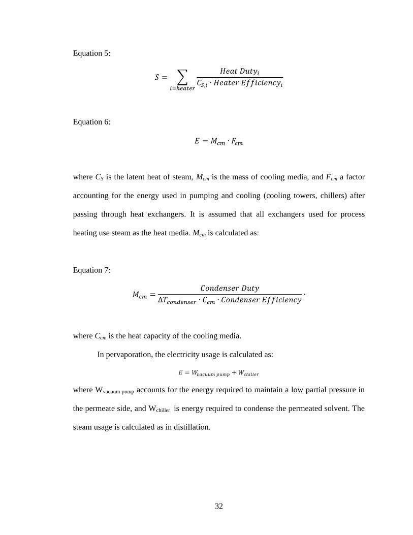
Recovery Process Utilities. Distillation steam, cooling media, and electricity

usage are determined with the resulting heat duties from Aspen Plus®

. The mass of steam

and electricity used in the recovery process is calculated as:

32

Equation 5:

∑

Equation 6:

where CS is the latent heat of steam, Mcm is the mass of cooling media, and Fcm a factor

accounting for the energy used in pumping and cooling (cooling towers, chillers) after

passing through heat exchangers. It is assumed that all exchangers used for process

heating use steam as the heat media. Mcm is calculated as:

Equation 7:

where Ccm is the heat capacity of the cooling media.

In pervaporation, the electricity usage is calculated as:

where Wvacuum pump accounts for the energy required to maintain a low partial pressure in

the permeate side, and Wchiller is energy required to condense the permeated solvent. The

steam usage is calculated as in distillation.

33

Pervaporation Modeling. The transport equation used to calculate the flux of a

component (Ji) across a pervaporation membrane is:

Equation 8

( ) [ ( ⁄ ) ( ⁄ ⁄ )]

This equation accounts for the effect of feed concentration and temperature, where f(xs)

accounts for the effect of organic solvent feed mass composition, Ei is the activation

energy of component i, R’ is the universal gas constant, TO is the reference temperature at

which the function f(xs) is derived, and TF is the feed temperature. The exponential

function represents the Arrhenius nature dependence of flux with temperature at a given

feed composition49,50

. f(xs) is a polynomial function of the feed mass fraction of the

organic solvent, since the flux of a component i as a function of the organic solvent feed

mass composition at a constant temperature can be well represented by a polynomial

equation. The polynomial coefficients of f(xs) were developed using experimental data on

commercially available membranes from the literature. These coefficients are membrane

and compound specific. The energy of activation of a component (Ei) is also dependent

on the membrane and on the other components present in the mixture and was derived

from experimental data as well.

Previous pervaporation models are based on the solution-diffusion

theory42,45,46,47,48

. Our model relies primarily on experimental data. The use of empirical

approaches over mass transfer models is not uncommon in chemical engineering, such as

in the rules of thumb used for the determination of height equivalent to theoretical plate

(HETP) in packed towers used for distillation51

.

34

Along a pervaporation unit, the temperature and mass composition in the liquid side

change since the temperature decreases due to water evaporation and the solvent gets

more concentrated as the water is continuously permeated. Accordingly, the flux across

the membranes changes as well, as suggested by Equation 8. To account for these

changes, the pervaporation membrane is divided into differential elements which

physically represent small segments of equal area, as seen in Figure 10. Pervaporation is

modeled in a cascade mode, in which the retentate of each area segment is sent to the

next area segment as the new feed. The permeate streams, on the other side, are collected.

To model an entire pervaporation unit, a mass and energy balance must be solved in each

subsequent area segment, until the desired purity of the retentate, concentrated in organic

solvent, is achieved. The procedure used to calculate the required membrane area to

achieve a desired purity is shown next. The equations referenced in this procedure are

included in Table 3.

1. As the starting point, the feed flow rate (F), temperature (T1), mass composition

(xs,1) must be defined. The compound properties and the area of the differential

segments (A) are already defined in the PV Simulator.

2. T1 and xs,1 are used in equations 9 and 10 to calculate the solvent and water flux,

Js,1 and Jw,1.

3. The total flux, J1, and permeate, P1, are calculated with Equation 11.

4. Equation 12 is used to calculate the retentate, R1.

5. Equation 13 is used to calculate the solvent mass fraction of the retentate, xs,2.

6. The solvent and water properties are used in Equation 14 to calculate T2.

35

7. At this stage, the data needed to calculate the mass and energy balance of the next

area segment are available: T2, xs,2, A, R1 and the solvent and water properties.

8. These steps are repeated as needed to achieve the desired purity, xs,T, being T the

total number of area block required.

A diagram representation of this procedure can be seen in Appendix E.

Equation 14 was adapted from Ho & Sirkar52

and Noble & Stern53

. This procedure to

design an industrial pervaporation unit as a continuous flow cascade process agrees with

Noble & Stern53

, Lipnizki et al.46

and Csefalvay et al.42

.

A1 A2 A3 ... AN

P1 P2 P3 ... PN

F,T1R1,T2 R2,T3 R3,T4 ... RN,TN+1

Figure 10. Differential elements (area segments) in a pervaporation membrane. R:

Retentate, P: Permeate, F: Feed, T: Retentate temperature. A: differential elements area

(A1 = A2 = A3 = … = AN = A).

Table 3. Equations used in the required pervaporation membrane area calculation

procedure

Equation Equation #

( ) [ ( ⁄ ) ( ⁄ ⁄ )]a 9

( ) [ ( ⁄ ) ( ⁄ ⁄ )]a 10

11

12

( ) ⁄ 13

36

(

) (

) ( )

a

14

a. Notation previously not defined:

and : heat of vaporization of the organic solvent

and water, respectively, at temperature TN; and

: heat capacity of the organic solvent and

water, respectively, at temperature TN.

Industrial pervaporation units contain modules with an already defined membrane

area. Therefore, the total area of the pervaporation unit will not be the summation of the T

number of area segments, but rather the minimum multiple of the industrial membrane

modules area that contains this summation. For example, if the total area required to

achieve certain purity is 51 m2 and the modules have an area of 35 m

2, two modules

would be required and the total area of the pervaporation unit would be 70 m2. The final

retentate flow rate and mass composition will be that of the last area segment of the

pervaporation unit.

Pervaporation energy requirements are to maintain a low partial pressure of the

permeating component in the permeate side, and heating the retentate to prevent a

drastically reduction in flux. In our model, pervaporation is induced by vacuum on the

permeate side generated with a vacuum pump. Because of the temperature decrease of the

retentate and the consequent reduction in flux, heating is typically used between

membrane modules38,50

. The tool assumes the use of inter-module heaters, being the

outlet temperature the same as the feed temperature.

The effect of concentration polarization has not been considered in the PV

Simulator, although its effect in pervaporation has been reported to be small40,53

. The

effect of swelling is assumed to be already considered in the experimental data. The

effect of neither permeate nor retentate pressure is considered. Our pervaporation model

37

was used within the experimental mass composition ranges. As for boundary conditions,

the flux of water and organic solvents approaches zero when the organic solvent mass

fraction in the retentate side approaches one.

When deriving the polynomial coefficients of the polynomial function f(xs), three

boundary conditions need to be considered: water and solvent flux is zero when solvent

mass composition in the feed/retentate is 1, and solvent flux is zero when solvent mass

composition in the feed/retentate is 0. The following procedure ensured that these

boundary conditions were fulfilled in the fitting curve:

1. A preliminary polynomial fitting curve was developed with all experimental

points.

2. A number of points equal to the power of the polynomial equations plus one were

selected, ensuring that the lower and higher solvent mass composition (the higher

being 1) points were selected.

3. A new fitting curve with the experimental points selected in step 2 was developed.

4. The coefficient of determination was calculated to indicate how well the new

curve fitted all the experimental points.

5. If the coefficient of determination was acceptable (>0.9), the fitting curve was

accepted, otherwise, the process went back to step 2.

Figure 11 shows an example of an original and revised fitting curve of the IPA flux

through a Sulzer’s membrane PERVAP 2201 in the dehydration of IPA.

38

Figure 11. IPA flux across Sulzer’s PERVAP 2201 pervaporation membrane as a

function of IPA mass fraction in the feed. Adapted from Qiao et al.54

.

Furthermore, the PV simulator does not model pervaporation below the

experimental range of solvent mass composition. When the experimental range did not

approached a solvent mass composition close to 1 (as in the case of IPA in membrane

PERVAP 2201), an artificial point of zero flux was included for both water and solvent at

a solvent mass composition of 1.

How to Use it. The steps for designing and optimizing a solvent recovery process

are: 1) define base case, 2) define recovery process, 3) simulate separation and optimize

distillation (if distillation is part of the recovery process), and 4) obtain final results. The

main inputs and results of each step are shown in Table 4.

0

0.001

0.002

0.003

0.004

0.005

0.006

0.8 0.82 0.84 0.86 0.88 0.9 0.92 0.94 0.96 0.98 1

IPA

Flu

x (k

g/m

2 h)

XIPA

Selected experimental points

All experimental points

Revised Fitting Curve

Original Fitting Curve

R2original = 0.988

R2revised = 0.982

39

Table 4. Main inputs and results of the simulation tool

Inputs

1) Define Base Case 2) Define Recovery Process

Waste and Costs Utilities Distillation Pervaporation

binary mixture

components

mass

composition

waste

management

method

waste

transportation

distance

transportation

type

total waste

(yearly basis)

solvents cost

utilities cost

Steam

characteristics

(pressure,

temperature,

saturation? etc.)

Cooling media

characteristics

(cooling media

energy factor,

heat capacity,

etc.)

desired purity

number of stages

feed stage

reflux ratio

feed flow rate

feed pressure

feed temperature

heat exchangers

efficiency and

heat integration

solvent to

dehydrate

mass

composition

flow rate

feed temperature

membrane type

module area

adiabatic or

isothermal

process

desired purity

heat exchangers

efficiency and

heat integration

Results

General Distillation Pervaporation

steam use

electricity use

purity achieved

stream mass flow rates

stream temperatures

life cycle emissions

avoided

operating cost

savings

Column

diameter

membrane

area required

By defining the base case we define all the information necessary to define the

LCIs that will be used to calculate the life cycle emissions avoided (Equation 3), and the

cost information that will be used to determine the operating cost savings (Equation 4).

Then, R.SWEET requires information of distillation and pervaporation to define how the

recovery process will be simulated. Finally, the results of the simulation are the missing

data to calculate the life cycle emissions avoided (Equation 3) and the operating cost

savings (Equation 4).

40

Once we obtain the results of our first simulation, we ask ourselves: “How do we

know that we have selected the best feed stage or reflux ratio?” To answer this question,

sensitivity analysis are available to maximize the operating cost savings and the life cycle

emissions avoided.

The ASW can be used to run multiple scenarios simultaneously to perform a

sensitivity analysis with the feed stage and reflux ratio as the independent variables. The

life cycle emissions avoided and operating cost savings are calculated for each scenario.

Then, R.SWEET highlights the optimum reflux ratio and feed stage that maximizes the

life cycle emissions avoided and operating cost savings. By selecting these parameters,

different recovery scenarios can be examined. Distillation optimization is valuable since

it is the most common solvent recovery process in the chemical industry55

. The sequence

for distillation optimization is shown in Figure 12.

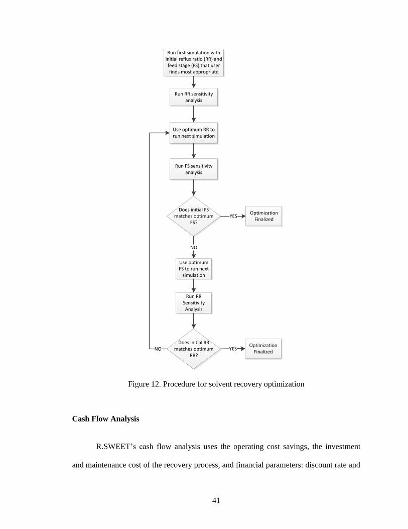
41

Figure 12. Procedure for solvent recovery optimization

Cash Flow Analysis

R.SWEET’s cash flow analysis uses the operating cost savings, the investment

and maintenance cost of the recovery process, and financial parameters: discount rate and

Run RR sensitivity analysis

Use optimum RR to run next simulation

Run first simulation with initial reflux ratio (RR) and feed stage (FS) that user finds most appropriate

Run FS sensitivity analysis

Does initial FS matches optimum

FS?YES

NO

Optimization Finalized

Use optimum FS to run next

simulation

Run RR Sensitivity Analysis

Does initial RR matches optimum

RR?YES

Optimization Finalized

NO

42

income tax, to returns three parameters used to financially evaluate projects: net present

value (NPV), internal rate of return (IRR) and payback period.

Comparison with Other Tools

Both Ecosolvent and our toolbox are used to environmentally assess the recovery of

solvents in waste mixtures by comparing the recovery scenarios to other waste disposal

methods, following a life cycle approach. However, the main differences reside in the

following additional capabilities of our toolbox:

Recommends recovery processes;

Simulate recovery processes;

Includes pervaporation;

Performs economic analyses.

Ecosolvent’s environmental analysis on distillation is performed with information

provided by the user, such as steam and electricity use, or, if this information is missing,

uses representative data; but does not run active simulations. Furthermore, our simulation

tools have the option to customize the type of steam and electricity used, in order to

generate a more representative LCI of a specific chemical plant. Nevertheless, Ecosolvent

offers greater detail regarding waste management methods other than waste recovery,

such as incineration. Therefore, our toolbox contains incineration LCI’s that were

obtained from Ecosolvent.

FIZ CHEMIE Berlin, provider of online database products for organic and industrial

chemists, developed a software tool that, given a binary mixture, recommends separation

processes and finds a suitable entrainer in the case azeotropic distillation is needed56

. This

43

software is comparable to our Recovery Process Selection Guide tool; however, it does

not include pervaporation as an alternative separation process. Furthermore, it does not

consider the mass composition of the components in the mixture, which has an impact on

recovery process design. Nevertheless, we acknowledge that an entrainer selection guide

is very useful tool when pervaporation is not applicable.

44

Chapter 3

Case Studies

Four solvent waste case studies were provided by Pfizer: 1) a mixture of acetone

and acetonitrile from the manufacture of selamectin, the API of the drug Revolution®

; 2)

an IPA and THF system derived from the production of API Nelfinavir, for the drug

Viracept®

3) the production of API hydrocortisone, for the drug TriOptic-S®

, generated a

toluene and acetone waste solution; and 4) a waste mixture of IPA and water from the

API celecoxib of the drug Celebrex®

. These cases were environmentally and

economically analyzed with our toolbox. More detail on the case studies is provided in

Table 4. As mentioned earlier, the adequate recovery process depends on the

thermodynamics behavior of the binary mixture. The acetone and acetonitrile

(selamectin), IPA and THF (nelfinavir), and toluene and acetone (hydrocortisone)

mixtures are homogeneous and do not form an azeotrope; therefore, distillation will

suffice as a separation process. IPA and water (celecoxib) forms a homogeneous liquid

mixture as well, but it presents an azeotrope at an IPA mass composition of 87.8 % wt.,

making distillation alone unable to purify IPA. Therefore, a pervaporation unit after

distillation was added for the fourth case study. These cases were selected to show the

flexibility of the proposed skid and of the simulation tool since they are representative of

high and low volume waste streams with different thermodynamic behavior. All the case

studies contain solvents that are widely used in the pharmaceutical industry. Therefore,

their evaluation sets a good basis for other manufacturing plants.

45

Table 5. Solvent waste case studies summary

Case Studya Selamectin Nelfinavir Hydrocortisone Celecoxib

Binary

Composition

(%wt.)

Acetonitrile (72)

& Acetone (28)

IPA (86) &

THF (14)

Toluene (91) &

Acetone (9)

IPA (50) &

Water (50)

Drug Revolution®

Viracept®

TriOptic-S®

Celebrex®

Mass of Solvent

Waste (kg/yr) 84,500 (LVWS)

78,700

(LVWS)

257,600

(LVWS)

5,470,000

(HVWS)

Solvent Cost

(US$/kg)

Acetone: 1.03

Acetonitrile:

4.07

IPA: 1.49

THF: 2.97

Toluene: 0.92

Acetone: 1.03

IPA: 0.92

Water: NA

Desired Recovery

Acetonitrile,

Acetone

(98 wt. %)

IPA

(98 % wt.)

Toluene

(99.8 wt. %),

Acetone

(98 wt. %)

IPA

(99.5 wt. %)

Waste

Management Cost

(US$/kg)

0.129 0.129 0.129 0.5

Utilities Cost

(US$/kg,

*US$/kWh)

Steam: 0.02

Electricity: 0.1

Steam: 0.02

Electricity:

0.1

Steam: 0.02

Electricity: 0.1

Steam: 0.04

Electricity:

0.127

Base Case Waste

Management

Method

Incineration for

Energy Recovery

Incineration

for Energy

Recovery

Incineration for

Energy

Recovery

Incineration

for Energy

Recovery

Recovery Process Distillation Distillation Distillation Distillation +

Pervaporation

Recovery Skid

Investment (US$)

1,500,000 1,500,000 1,500,000 2,960,000

Combined: 1,500,000

All cases combined: 2,960,000 a: Case studies are named after the API manufactured from which the solvent waste is generated.

The Skid

The ultimate goal was to design a skid of relatively low capital investment cost,

small footprint, and be versatile enough so that it can be used to treat different solvent

streams. Such a system would allow for the recovery and reuse of multiple organic

solvent streams, making the original capital investment viable. This concept fits very well

46

with the batch-and nature of the manufacturing process in pharmaceutical companies.

This skid would then be used as the equipment for solvent recovery simulation in all the

case studies. Such recovery unit would be flexible enough to purify all solvent waste case

studies, minimizing idle time. Finally, the skid would break the solvent recovery barrier:

plant not fit for solvent recovery.

The design of this skid resulted in the following characteristics:

A structured packed distillation column of 20 ft. of height and 1.5 ft of diameter.

Assuming a maximum HETP of 2 ft.57

, this column would contain at least 10

theoretical stages

The type of packing selected in Aspen Plus®

was MellapakPlusTM

252.Y from

Sulzer Chemtech. A packed column was selected for distillation because it is

recommended for the diameter and operating pressure considered. Furthermore,

as compared to trayed and randomly packed columns, structured packed towers

usually have less residence time, which minimizes thermal degradation and

pressure drop and allow for less height since they are more efficient58

.

As for pervaporation, a unit using Sulzer’s PERVAP®

2510 membranes with an

area of 210 m2 was considered which accounts for 6 modules of 35 m

2 each. We

based this design on the commercially available Sulzer plate and frame system,

because this type of pervaporation equipment is available at a Pfizer plant in

Barceloneta, where one of the solvent waste case studies was generated. The

membrane is composed of a polyvinyl alcohol polymer.

The estimate dimensions for the skid including auxiliary equipment (pumps,

pipes, tanks, and heat exchangers) are 15 ft. x 15 ft. x 35 ft. in W x D x H. These

47

approximate dimensions where obtained from distillation tower vendor quotations

and from similar existing pervaporation units at chemical plants. Furthermore, the

skid would address the problem mentioned in the introduction regarding the

difficulty to implement solvent recovery due to the lack of consistency with

existing facilities. - Can be used indoor.

Skid Economics. The economic feasibility of using the recovery skid in each case

was investigated with a cash flow analysis. The equipment cost estimation for the

distillation system was obtained as the average of three vendor quotations. The

installation costs were assumed to be 100 % of the capital cost, resulting in a total

investment cost for each selamectin, nelfinavir and hydrocortisone case of US$

1,500,000. If the same recovery skid was used for the three cases, the cost would be the

same as the individual value. It should be noted that these three case studies occurred at

the same manufacturing plant. The equipment and installation cost of a pervaporation

unit with a membrane area of 210 m2 was determined to be US$ 1,460,000. Therefore,

the investment cost for the Celecoxib case skid would be US$ 2,960,000. A membrane

lifetime of 3 years was obtained from Van Hoof et al.35, as well as a polymeric

membrane cost of US$740/m2, which would account for US$ 155,400 in our

pervaporation unit. All pervaporation costs were obtained from Van Hoof et al.35, and

adjusted based on the actual size of the equipment in our model. All the costs were

updated to current date with the average inflation rate from the date of the reference to

the date of the paper submission, obtained from Trading Economics59

. If a recovery skid

48

would be used for the four cases, the investment cost would be that of the celecoxib case.

A detailed calculation of the recovery skid can be seen in Appendix J.

It is interesting to note that idle equipment suitable for solvent recovery could be

available at an API manufacturing plant, in which case the investment cost could be

lower.

General Considerations

The following procedures, assumptions and conditions were applied to all of the case

studies evaluation.

All the cases were provided by Pfizer.

The base case waste management method is incineration for energy recovery in a

cement kiln, as all the cases analyzed in this research used a similar method.

All the cases were evaluated with R.SWEET. R.SWEET was used to simulate the

distillation recovery process, calculate the life cycle emissions reduction and the

operating cost savings.

The distillation column reflux ratio and feed stage that maximized the life cycle

emissions avoided was selected using R.SWEET.

The feed temperature to the distillation column is 35 °C.

The life cycle emissions (LCE) of the reflux pump energy and for the

manufacture of the recovery process equipment were not considered.

Heat exchangers have an efficiency of 90 % and heat integration was not

considered.

Waste transport emissions are zero.

49

Cooling water was the cooling media. In Equation 7 average cooling water temperature

temperature change of 5 °C, and the heat capacity of water is 4.184 kJ/(kg·°C). In

Equation 6 the cooling water electricity factor (Fcm) is 1.71 kWh per ton of

cooling water;

In the distillation column, an atmospheric operating pressure was selected to

minimize thermal degradation and operating costs.

In a conservative approach, 8 theoretical stages were used in all case studies, even

though 10 stages are available.

The flow rate to the distillation column was selected to obtain a column diameter

of 1.5 ft, which is the skid’s distillation column diameter.

For the cash flow analysis, the annual maintenance costs of the skid were assumed

to be 2.5 % of the total capital cost. The internal rate of return (IRR) was

determined for a period of 10 years. An income tax rate of 35 % was considered

for the cash flow analysis.

Selamectin Case: Acetone and Acetonitrile

Overview. The first homogenous binary solvent system investigated was an

acetonitrile and acetone waste mixture. This case study has been provided by Pfizer, Inc.

from their Kalamazoo, Michigan plant. This mixture is a waste stream from the

production of selamectin (the active ingredient in the drug Revolution®

) that contains 72

% wt. acetonitrile in acetone. Selamectin is the API in the drug Revolution®

; a topical

monthly parasite treatment for both cats and dogs. The final drug formulation is

composed of isopropyl alcohol, dipropylene glycol methyl ether, and selamectin which

50

makes up between 7-14% of the total composition of the drug.60

Revolution®

is effective

in killing a number of different parasites, such as fleas and a variety of worms. The drug

also controls ear mite, sarcoptic mange, and tick infestations. The drug is applied

topically, absorbed through the skin, and is distributed throughout the body by means of

the bloodstream.61

Selamectin has a molecular weight of 770 g/mol and formula C43H63NO1162

.

According to the current patent, the process for preparing selamectin is comprised of four

major steps. The first step is the catalytic hydrogenation of doramectin in acetone. This

intermediate step yields 25-cyclohexyl-22,23-dihydroavermectin. This product is isolated

by filtration and separated from the acetone. Step two involves oxidation of this product

in the presence of manganese dioxide in an organic solvent to yield 25-cyclohexyl-22,23-

dihydro-5-ovoavermectin. This product may or may not be crystallized depending on the

process and the key intermediate. Step three is the reaction of this product with

hydroxylamine hydrochloride. This produces the final product. Step four consists of

purifying the product by crystallization from toluene. The product is then dried to a

powder under a vacuum. The final product is 25-cyclohexyl-22,23-dihydro-5-

hydroyimino-avermectin, or selamectin. The yields are based on the activity of the

doramectin starting product and whether or not the product from step two is cystallized.63

In recent years, Pfizer has on a global basis recovered approximately 60 % of

solvents used, and incinerated approximately 40%. A significant portion of this 40 % is

not typically recovered because the individual stream volumes are between 10,000 to

20,000 gallons, which is too small for existing solvent recovery systems. The acetone-

acetonitrile waste stream was selected for this conceptual study because it had the most

51

economic value and the highest potential for both economic and environmental savings,

from a list of such smaller volume waste streams being generated at the time.

Two process waste streams, resulting from a step in the production of an

intermediate (called SEL), contain recoverable acetonitrile and acetone that must be

separated before reuse. Both streams are distillate waste streams, and are combined to

form a stream containing 28 % wt. acetone and 72 % wt. acetonitrile at ambient

conditions. Figure 13 shows the output of step 1 for making the API and the waste stream

specific to the production of selamectin. Table 6 contains the process specifications,

which are based on the combined waste stream to be processed by the recovery system in

Figure 13.

Figure 13. Simple PFD for waste recovery of acetonitrile/acetone. The green square

highlights the location of the proposed recovery in the API manufacturing process.

Materials fromPrior processing

Processing of SEL Intermediate

Distillation

Proposed Recovery System

Distillation

Additional processing

(Washing, Drying, Filtering)

SELacetone

Acetonitrile

acetone

To recycleAcetonitrile-pure

stream

Acetone-purestream

Acetone

To offsiterhodium recovery

To offsitecold storage

AcetonitrileAcetoneN2 gas

52

Table 6. Selamectin case waste stream characterization

Acetone Acetonitrile

Mass Fraction 0.28 0.72

Mole Fraction 0.22 0.78

Volume Fraction 0.28 0.72

Purchase Cost (US$/kg) 1.03 4.07

Incineration Cost (US$/kg) 0.129 Total

Mass (kg/yr) 23,660 60,840 84,500

Cost (US$/yr) 24,370 247,619 271,989

Acetonitrile is a commonly used solvent in many organic and inorganic syntheses.

According to the 2010 TRI, acetonitrile ranks fourth for chemical wastes generated by the

pharmaceutical and medicinal sectors. Acetone is another common solvent used in the

pharmaceutical industry. Acetonitrile is usually acquired as a by-product of the propylene

ammoxidation process for acrylonitrile production.64

This solvent has favorable

properties for many chemical reactions. Some of these properties of acetonitrile are low

acidity, low boiling point, low viscosity, and low chemical reactivity.65

Beginning in fall of 2008, a worldwide shortage of acetonitrile developed. The

shortage caused prices for acetonitrile to rise drastically. One of the largest factors

affecting the acetonitrile shortage is the current state of the economy. Acrylonitrile is

used in manufacturing non-essentials, such as automobiles, carpets, acrylic and carbon

fibers, luggage, small appliances, telephones, computer housings, and other products.

Since the demand for these commodities has decreased, so has the production of

acrylonitrile and thus acetonitrile65

.

Table 7 shows different environmental indicators of acetonitrile and acetone. The

physical and chemical properties of acetone and acetonitrile are listed in Table 8.

Acetonitrile and acetone are fully miscible in each other and in water.

53

Table 7. Acetonitrile and acetone toxicity and environmental exposure limits

Solvent TLVa

PELb

LC50c

LD50d

Carcinogenicity

Acetonitrile 20 ppm

40 ppm 7.551 g/m

3

8 hours (Rat)

50 mg/kg

(Rabbit)

EPA Group D (Inadequate

evidence for human cancer)66

Acetone 500 ppm 1000 ppm 44 g/m

3

4 hours (Mouse)

5340 mg/kg

(Rabbit)

EPA Group D (Inadequate

evidence for human cancer)67

a The Threshold Limit Value (TLV) is the amount of a substance that an individual can be exposed to for 8

hours a day and 5 days a week, without adverse health effects. b The Permissible Exposure Limit (PEL) is the legal limit in the United States for the exposure of an

individual to a substance. c The discharge limits are given in LC50, which is the lethal concentration of a chemical in the air that kills

half of the population. d The LD50 is the lethal dose of a substance that is required to cause death to half of the tested population.

Table 8. Physical and chemical properties

Solvent Molecular

Weight

Density at

25°C

Solubility in

water (g/100g)

Boiling Point

at 1 atm

Acetonitrile 41.05 g/mole 0.781 g/mL Miscible 81.6°C

Acetone 58.08 g/mole 0.786 g/mL Miscible 56.5°C

Thermodynamic Evaluation and Recovery Process Design. A T-x-y and x-y

equilibrium diagrams for the acetone-acetonitrile system is provided in Figure 14 and

Figure 1568

. These diagrams show the absence of an azeotrope, therefore distillation is a

viable separation option. The required purity for reuse is 98 wt. % for both solvents.

Because the conceptual skid has only one distillation column, the recovery of acetone and

acetonitrile cannot be performed simultaneously. It was tried to accomplish but the 8

stages of the skids distillation column were not sufficient. The recovery of acetonitrile

through the bottoms of the distillation was simulated first because it is the target solvent.

Distillation bottoms products usually contain more impurities than distillates, but it

should be reminded that both acetone and acetonitrile streams that compose the final

waste mixture come from distillates. The distillate of the first recovery was used later to

54

recover acetone in the same column. The proposed recovery scheme is presented in

Figure 16.

Figure 14. Vapor-liquid equilibrium T-x-y diagram for acetone and acetonitrile at P = 1.0

atm. Generated in Aspen Plus®

with UNIQUAC.

Figure 15. Vapor-liquid equilibrium x-y diagram for acetone and acetonitrile at P = 1.0

atm. Generated in Aspen Plus®

with thermodynamic property method UNIQUAC.

55

60

65

70

75

80

85

0 0.1 0.2 0.3 0.4 0.5 0.6 0.7 0.8 0.9 1

Tem

per

ature

( C

)

Acetone Mass Fraction

Vapor

Liquid

0

0.1

0.2

0.3

0.4

0.5

0.6

0.7

0.8

0.9

1

0 0.1 0.2 0.3 0.4 0.5 0.6 0.7 0.8 0.9 1

Ace

tone

vap

or

mas

s fr

acti

on (

y)

Acetone Mass Fraction in Liquid (x)

55

Figure 16. Acetonitrile and acetone recovery scheme in the selamectin case.

Life Cycle Assessment. LCIs for the production and incineration of both

acetonitrile and acetone were obtained from SimaPro®

and Ecosolvent, respectively.

Detailed information regarding acetone and acetonitrile manufacture and incineration

LCI’s is included in Appendix F. The total emissions for the production of the solvent

were opened up in three categories; emissions to air, soil, and water. Major pollutants in

each category are shown. Emissions to air include CO2, carbon monoxide (CO), nitrogen

oxides (NOx), non-methane volatile organic compounds (NMVOCs), particulates, and

sulfur dioxide (SO2). Specified emissions to water are volatile organic compounds

(VOCs).

The total emissions to the environment for the production of 1 kg of acetone are

1.86 kg. This value is driven by air emissions, which total 1.83 kg. CO2 constitutes 98 %

of the air emissions with other gases, mostly methane, a greenhouse gas, comprising the

remaining 2 %. The total emissions from the manufacture of acetonitrile are 2.12 kg per

kg of acetonitrile, comparatively larger than the 1.86 kg of emissions from the

manufacture of 1 kg of acetone. Similar to the LCI for acetone, 93% of the total

Waste

Mixture:

Acetone

(28 wt. %)

Acetonitrile

(72 wt. %)

A B

Acetonitrile

(98 wt. %)

Acetone

(98 wt. %)

A: First

Distillation

B: Second

Distillation

Solvent

Waste

56

emissions are released to air. 1.95 kg of the 1.97 kg of total air emissions are attributed to

CO2. The other 0.2 kg is made up of a variety of gases, mostly greenhouse gases. The

process that is used in the SimaPro®

calculation for the emissions of acetonitrile is the

SOHIO process, where acetonitrile is actually a by-product of the production of

acrylonitrile. Nearly all of the acrylonitrile produced in the world today is produced using

the SOHIO process. The primary by-products of the process are hydrogen cyanide,

acetonitrile, and carbon oxides.69

Both manufacturing processes have high Cumulative Energy Demand (CED). The

CED includes energy from both renewable resources such as water, wind or solar, and

biomass, and non-renewable energy such as nuclear or fossil fuels. To make 1 kg of

acetone and 1 kg of acetonitrile, 64.8 MJ-Eq and 58.6 MJ-Eq of energy are required,

respectively.

LCIs were developed for the utilities used by the Kalamazoo plant in SimaPro®

.

These utilities LCIs will be included in R.SWEET to model recovery processes in the

Kalamazoo plant: Selamectin Case, Nelfinavir Case and Hydrocortisone Case. The

detailed LCI for the Kalamazoo utilities can be seen in Appendix G.

Nelfinavir Case: IPA and THF

Overview. Nelfinavir Mesylate (Nelfinavir) is the API in the drug Viracept®

.

Viracept®

is an antiretroviral protease inhibitor that is used in the treatment of the human

immunodeficiency virus (HIV). The final drug formulation is composed of calcium

silicate, colloidal silicon dioxide, magnesium stearate, and Nelfinavir which makes up

between 47-61% of the total composition of the drug.

57

Nelfinavir has a molecular weight of 568 g/mol and formula C32H45N3O4S. 70,71

According to the chemical’s MSDS, as of 2009 the environmental effects of Nelfinavir

have yet to be determined. It is suggested that any releases to the environment should be

avoided.71

The nelfinavir waste stream studied was composed of 86 % wt. isopropyl alcohol

(IPA) and 14 % wt. tetrahydrofuran (THF). The IPA in this waste stream must be

recovered at 98 % wt. purity to be reused. Table 9 contains the solvent waste

specifications.

Table 9. Nelfinavir waste stream characterization

IPA THF

Mass Fraction 0.86 0.14

Purchase Cost(US$/kg) 1.49 2.97

Incineration Cost (US$/kg) 0.129 Total

Mass (kg/yr) 67,682 11,018 78,700

Cost (US$/yr) 100,846 32,723 133,569

THF is a common solvent used in the pharmaceutical industry. IPA has favorable

properties for many chemical reactions, including the ability to quickly dissolve non-

polar compounds, low toxicity, and quick evaporation capability.72

Table 10 shows

different environmental indicators for IPA and THF. Physical and chemical properties of

IPA and THF are listed in Table 11. IPA and THF are fully miscible.

58

Table 10. IPA and THF environmental exposure limits and toxicity information

Solvent TLVa

PELb

LC-50c

LD-50d

Carcinogenicity

IPA73

400 ppm 500 ppm

16000 mg/kg

8 hours (Rat)

3600 mg/kg

(Mouse)

IARC Group 3 (Not

cancerous to humans)

THF74

250 ppm 250 ppm 24 g/m

3

4 hours (Mouse)

1650 mg/kg

(Rat)

Group D (Inadequate

evidence for human cancer) a The Threshold Limit Value (TLV) is the amount of a substance that an individual can be exposed to for 8

hours a day and 5 days a week, without adverse health effects. b The Permissible Exposure Limit (PEL) is the legal limit in the United States for the exposure of an

individual to a substance. c The discharge limits are given in LC50, which is the lethal concentration of a chemical in the air that kills

half of the population. d The LD50 is the lethal dose of a substance that is required to cause death to half of the tested population.

Table 11. IPA and THF physical and chemical properties

Solvent Molecular

Weight

Density at

25°C

Solubility in

water (g/100g)

Boiling Point at

1 atm

IPA 60.1 g/mole 0.79 g/mL Miscible 82.5°C

THF 72.11 g/mole 0.89 g/mL Miscible 66.1°C

Thermodynamic Evaluation and IPA Recovery Process Design. A T-x-y and

x-y equilibrium diagrams for the IPA-THF system are provided in Figure 17 and Figure

18, respectively68

. As can be seen, the solution forms a homogeneous non-azeotropic

mixture. At the vicinity of a THF mass fraction of 1, the relative volatility of both

components is close to 1, making the vapor and liquid equilibrium lines to be very close

to each other. This suggests that distillation is not a viable separation option for obtaining

high purity THF. The vapor-liquid equilibrium close to an IPA mass fraction of 1 is

favorable for distillation, which means that high purity IPA can be obtained with this

separation technique. The separation scheme for the nelfinavir case is shown in Figure

19.

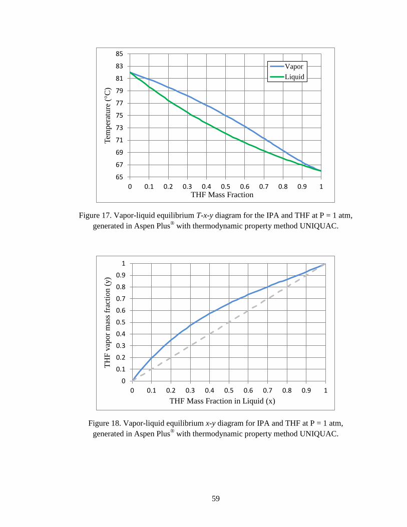
59

Figure 17. Vapor-liquid equilibrium T-x-y diagram for the IPA and THF at P = 1 atm,

generated in Aspen Plus®

with thermodynamic property method UNIQUAC.

Figure 18. Vapor-liquid equilibrium x-y diagram for IPA and THF at P = 1 atm,

generated in Aspen Plus®

with thermodynamic property method UNIQUAC.

65

67

69

71

73

75

77

79

81

83

85

0 0.1 0.2 0.3 0.4 0.5 0.6 0.7 0.8 0.9 1

Tem

per

atu

re ( C

)

THF Mass Fraction

Vapor

Liquid

0

0.1

0.2

0.3

0.4

0.5

0.6

0.7

0.8

0.9

1

0 0.1 0.2 0.3 0.4 0.5 0.6 0.7 0.8 0.9 1

TH

F v

apor

mas

s fr

acti

on (

y)

THF Mass Fraction in Liquid (x)

60

Figure 19. IPA recovery scheme in the nelfinavir case.

Life Cycle Assessment. The total emissions to the environment are 2.20 kg per 1

kg of IPA manufactured. Air emissions make up 1.66 kg of the total emissions with 1.63

kg of emissions from carbon dioxide. The total emissions from the manufacture of 1 kg

of THF are 5.65 kg. The majority of the emissions are released to the air. Air emissions

attributed to CO2 are 5.46 kg of the 5.52 kg of total air emissions. The remaining 0.06 kg

is made up of a variety of greenhouse gases and other pollutants. Both manufacturing

processes have a high CED. The manufacture of 1 kg of IPA and 1 kg of THF require

60.1 MJ-Eq and 128 MJ-Eq, respectively. For both THF and IPA, the majority of this

energy is supplied by non-renewable fossil fuels as seen in Appendix G.

The process that is used in the SimaPro®

calculation for the emissions of THF is

the manufacture of THF from 1,4-butanediol in Europe, while IPA is a readily available

organic solvent that is produced from the synthesis of water and propene. The detailed

LCIs for THF and IPA can be seen in Appendix F. The LCA for the base process is

detailed in Appendix H.

Waste

Mixture:

THF (14 wt. %)

IPA (86 wt. %)

Solvent Waste

(THF + IPA)

Distillation

Column

IPA

(98 wt. %)

61

Hydrocortisone Case: Toluene and Acetone

Overview. Hydrocortisone acetate is a topical, oral, or intravenous corticosteroid

which works to prevent inflammation. Inflammation or swelling is prevented by lowering

the formation, release, and activity of different cells and chemicals in the body.

Hydrocortisone is typically used for allergic reactions and skin conditions including

eczema, psoriases, and rashes. Hydrocortisone acetate has a molecular weight of 404.5

g/mol and a formula of C23H32O675

. Hydrocortisone acetate is an API in the drug TriOptic

S®

. TriOptic S®

is a treatment for bacterial infections in the eyelid and conjunctiva in

dogs and cats. The medication is administered 3-4 times daily in a thin film over the

cornea. The final drug formula is composed of bacitracin, neomycin, polymyxin, and

hydrocortisone acetate which makes up approximately 1% of the total composition of the

drug.76

TriOptic S is effective in bactericidal action against both gram negative and gram

positive bacteria which may infect the eye. TriOptic S®

combines the APIs found in

Trioptic P along with hydrocortisone acetate, which is an anti-inflammatory agent.

TriOptic S allows for bactericidal action and prevention of inflammation in the anterior

of the eye.

The process waste stream from the Kalamazoo plant production of hydrocortisone

acetate contains toluene and acetone which must be separated before reuse. The solvent

waste stream is composed of 79.3 % wt. toluene, 8.0 % wt. acetone, 10.0 % wt. water,

and 2.7 % wt. branched octane with trace cyanide at 30 ppm. Branched octane is a term

used by Pfizer which refers to an Exxon Mobile product called IsoparTM

C. Table 12

62

shows the process specifications for the solvents of interest in the process waste stream:

toluene and acetone.

Toluene is an organic solvent which is used in pharmaceutical syntheses because

of its solubility with APIs and intermediates. According to the TRI from 2010, toluene

ranks second for chemical wastes generated by the pharmaceutical and medicinal sectors

at 5,310,000 kg/year. Toluene is acquired as a byproduct of the production of fuels such

as gasoline and coke.

Environmental indicators for acetone and toluene are shown in Table 13.

Table 12. Hydrocortisone solvent waste stream characterization

Toluene Acetone

Mass Fraction 0.79 0.08

Mole Fraction 0.535 0.085

Volume Fraction 0.763 0.085

Purchase Cost (US$/kg) 0.92 1.03

Incineration Cost (US$//kg) 0.129 Total

Mass (kg/yr) 233,913 23,687 257,600

Cost (US$/yr) 215,200 24,398 239,598

Table 13.Environmental exposure limits for solvents from 5C waste stream

Solvent TLVa

PELb

LC50c

LD50d

Carcinogenicity

Acetone 500 ppm 1000 ppm 44 g/m

3

4 hours (Rat)

5340 mg/kg

(Mouse)

EPA group D (Inadequate

Evidence for human cancer)

Toluene 50 ppm 300 ppm 49 g/m

3

4 hours (Rat)

636 mg/kg

(Rat)

Group A4 (Not classifiable for

human) a The Threshold Limit Value (TLV) is the amount of a substance that an individual can be exposed to for 8

hours a day and 5 days a week, without adverse health effects. b The Permissible Exposure Limit (PEL) is the legal limit in the United States for the exposure of an

individual to a substance. c The discharge limits are given in LC50, which is the lethal concentration of a chemical in the air that kills

half of the population. d The LD50 is the lethal dose of a substance that is required to cause death to half of the tested population.

63

Physical and chemical properties of acetone and toluene are listed in Table 14.

Only acetone is fully miscible in water; however toluene and acetone are miscible in each

other.

Table 14. Physical and chemical properties for hydrocortisone’s case waste stream66

Molecular

Weight

Density at

25°C

Solubility

in water

(g/100g)

Boiling Point at

P = 1 atm

Acetone 58.08 g/mole 0.786 g/mL Miscible 56.5°C

Toluene 92.14 g/mole 0.86 g/mL 0.561 110.6°C

Thermodynamic Evaluation and Recovery Process Design. Water and

branched octane can be almost fully removed from the mixture by decanting. Additional

tanks and a decanter are required. After decanting, the waste stream contains only 0.8 %

wt. branched octane and 0.06 % wt. water. These small amounts allow for separation of

toluene and acetone by distillation. Therefore, the mixture was assumed to be binary for

the purpose of being evaluated with R.SWEET. For the toluene to be recycled back to the

process, the contaminants can only make up 0.02 wt. % of the recycled stream. On the

other hand, acetone’s mass purity specification for recycling is 98 wt. %. A T-x-y and x-y

equilibrium diagrams for the acetone-toluene system are provided in Figure 20 and

Figure 21. The absence of an azeotrope and the high relative volatility suggests that both

pure acetone and acetonitrile can be recovered through distillation. The recovery scheme

is shown Figure 22. As can be seen, one distillation suffices to recover both solvents. The

analysis performed to reach this conclusion is detailed in Chapter 4.

64

Figure 20. Vapor-liquid equilibrium T-x-y diagram for acetone and toluene at P = 1 atm.

Generated in Aspen Plus®

with thermodynamic property method UNIQUAC.

Figure 21. Vapor-liquid equilibrium x-y diagram for acetone and toluene at P = 1 atm.

Generated in Aspen Plus®

with thermodynamic property method UNIQUAC.

50

60

70

80

90

100

110

120

0 0.1 0.2 0.3 0.4 0.5 0.6 0.7 0.8 0.9 1

Tem

per

atu

re ( C

)

Acetone Mass Fraction

Vapor

Liquid

0

0.1

0.2

0.3

0.4

0.5

0.6

0.7

0.8

0.9

1

0 0.1 0.2 0.3 0.4 0.5 0.6 0.7 0.8 0.9 1

Ace

tone

vap

or

mas

s fr

acti

on (

y)

Acetone Mass Fraction in Liquid (x)

65

Figure 22: Toluene and acetone recovery scheme in the hydrocortisone case.

Life Cycle Inventory. The detailed LCIs for toluene and acetone are included in

Appendix F. The total emissions to the environment are 1.21 kg per 1 kg of toluene

manufactured. Air emissions make up almost all of the total emissions, with 1.19 kg of

emissions from CO2. Toluene manufacture requires 61.9 MJ-Eq of energy per kg. The

majority of this energy is supplied by fossil fuels as seen in Appendix G. The LCA for

the base process can be seen in Appendix H.

Celecoxib Case: IPA and Water

Overview. A solvent waste stream composed of isopropanol (IPA) and water is

produced from the manufacture of the Celecoxib, the API of the drug Celebrex®

. This

API is made at Puerto Rico and Singapore plants. In 2007, the Barceloneta plant in

Puerto Rico generated 5.5 kilotons of waste per year, containing mainly IPA, at 46.8 wt.

%, and water.

This solvent waste is generated from multiple waste streams, with varying

compositions of isopropanol, ethanol, methanol, water and dissolved solids. Because the

Waste

Mixture:

Acetone (9 wt. %)

Toluene (91 wt. %)

Toluene

(99.8 wt. %)

Distillation

Column

Acetone

(98 wt. %)

66

presence of lower alcohols was in small concentrations, for the purpose of this study, the

waste was simplified to an IPA and water binary system.

Thermodynamic Analysis and Recovery Process Design. Conventional

distillation is limited in obtaining pure IPA from the waste, since water forms an

azeotrope with IPA at 87.8 % wt. The azeotrope is not pressure sensitive, which limits the

use of pressure-swing distillation. The T-x-y and x-y vapor liquid equilibrium diagram

for IPA and water is provided in Figure 23 and Figure 24.

In 2008, a design case study has been performed by Rowan University with Pfizer

through a prior EPA grant, “Advancing P2 in Pharmaceutical Manufacturing”77

. The

manufacturing operation at their plant in Barceloneta, Puerto Rico, was evaluated and

several green engineering alternatives for the purification and recovery of isopropanol

from waste streams proposed. A conceptual study of distillation, extraction, reactive

distillation, adsorption, and membrane-based processes was performed. Several green

design approaches were evaluated using distillation combined with either molecular sieve

adsorption or membrane pervaporation. These process schemes appear to have the most

promise to effectively purify and recover isopropanol. In addition, the dehydration of

isopropanol has been extensively covered in scientific literature and a combination of

distillation and pervaporation units has been suggested for solvent recovery.35,54,78,

Distillation to the azeotrope was proposed as the first step in a sequential

separations train followed with a more advanced separation operation. Pervaporation is

one of several unit operations that can be used in combination with distillation in the

separation of azeotropic solvent mixtures. The recovery of isopropanol using distillation

followed by pervaporation was simulated and optimized using R.SWEET. The distillation

67

column was set to obtain a distillate with an IPA mass purity of 85 % wt., which was sent

to a pervaporation unit, set to obtain a mass purity of 99 % wt. The feed to the

pervaporation unit was heated from the distillate temperature of around 80 °C to 95 °C, in

order to increase mass transfer through the membrane. The inter-module heaters outlet

temperature was 95 °C as well. The flow rate to the pervaporation unit was determined as

the distillate flow rate in the celecoxib case, to ensure a continuous operation (the IPA

and water azeotrope is obtained in the distillate while water is obtained in the bottoms).

The recovery scheme of the celecoxib case is provided in Figure 25. A distillate

containing a composition of IPA 85 % wt. was obtained in the distillation column and

sent to the pervaporation unit to dehydrate the stream and achieve a 99.5 % wt. purity.

Figure 23. Vapor-Liquid Equilibrium T-x-y diagram for IPA and water at P = 1 atm

Generated in Aspen Plus®

with UNIQUAC

75

80

85

90

95

100

105

0 0,1 0,2 0,3 0,4 0,5 0,6 0,7 0,8 0,9 1

Tem

per

ature

( C

)

IPA Mass Fraction (x,y)

Vapor

Liquid

68

Figure 24. Vapor-Liquid Equilibrium x-y diagram for IPA and water at P = 1 atm.

Generated in Aspen Plus®

with thermodynamic property method UNIQUAC.

Figure 25. IPA recovery scheme in the celecoxib case.

Life Cycle Analysis. The manufacture and incineration LCIs of isopropanol and

ultrapure water are presented in Appendix F. The emissions due to the production of

isopropanol were estimated through the direct and indirect hydration of propylene.

The LCI of steam and electricity used at the Puerto Rico plant has already been

developed in the document “Advancing P2 in Pharmaceutical Manufacturing”. The LCI

0

0,1

0,2

0,3

0,4

0,5

0,6

0,7

0,8

0,9

1

0 0,1 0,2 0,3 0,4 0,5 0,6 0,7 0,8 0,9 1

IPA

vap

or

mas

s fr

acti

on (

y)

IPA Mass Fraction in Liquid (x)

Waste Mixture:

IPA (50 wt. %)

Water (50 wt. %)A

Water

IPA (retentate)

(99.5 wt. %)

A: Distillation

B: Pervaporation

Water

(permeate)

B

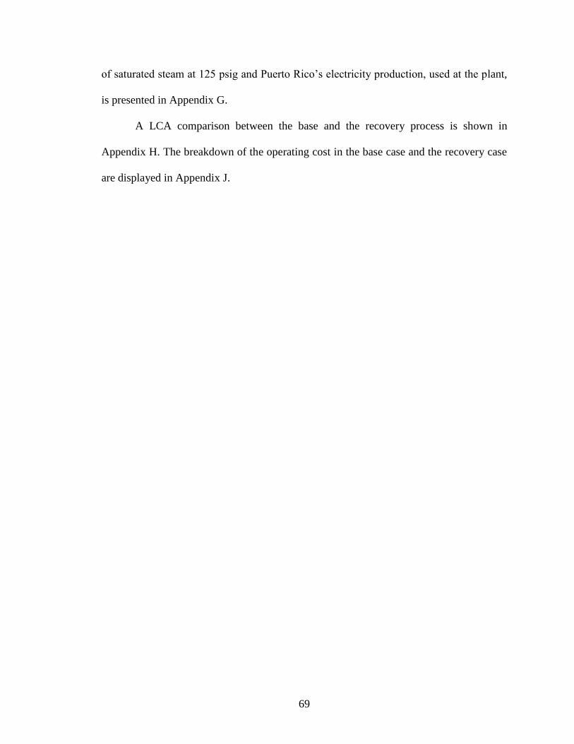
69

of saturated steam at 125 psig and Puerto Rico’s electricity production, used at the plant,

is presented in Appendix G.

A LCA comparison between the base and the recovery process is shown in

Appendix H. The breakdown of the operating cost in the base case and the recovery case

are displayed in Appendix J.

70

Chapter 4

Results and Discussion

The environmental and economic results of the case studies are summarized in

Table 15. Life cycle emissions avoided are calculated as the difference between the base

case and the recovery case life cycle emissions. Detailed results of the base case and

recovery case life cycle emissions and operating cost savings can be seen in Appendix H

and I, respectively. The graphical results of the distillation reflux ratio sensitivity

analyses (RRSA) are shown in Figure 26 to Figure 35, while the feed stage sensitivity

analyses are presented in Figure 27 to Figure 36. For the purpose of this study, a reflux

ratio increment of 1 was used in the RRSA, but shorter increments can be used in

R.SWEET to further refine the optimization.

In the selamectin case, the first distillation RRSA for the acetonitrile recovery

(Figure 26) shows a maximum LCE avoided (LCEA) at a reflux ratio of 9 and a

maximum operating cost savings (OCS) at a reflux ratio of 28. Albeit this difference, at

the maximum LCEA, the OCS are 95.1 % of the maximum OCS. In Table 15, the

optimum reflux ratio for all the cases corresponds to the one that maximizes LCEA.

However, both LCEA and OCS are positive at either maximum; therefore, the recovery

system can be operated between these reflux ratio ranges according to the pharmaceutical

company’s priorities. The meaning of the LCEA maximum is that as the reflux ratio

increases up to the maximum, the manufacture and waste incineration LCEA increase at a

higher rate than the recovery process emissions. After the maximum, the contrary occurs,

which is the reason of the maximum occurrence. This can be seen in Figure 28, in which

71

the slope of the manufacture and incineration LCEA curve is higher than the slope of the

recovery process emissions curve at a reflux ratio lower than 9, and lower at a reflux ratio

higher than 9. This means that the difference between the manufacture and incineration

LCEA and the recovery process emissions generated (Equation 3) are higher at a reflux

ratio of 9. The manufacture and incineration LCEA are directly proportional to the

recovery, since as more solvent is recovered, more LCE are avoided. This is the reason

why in Figure 28 the slope of the recovery curve and the manufacture and incineration

LCEA curve are the same. On the other hand, the steam and electricity use are directly

proportional to the reflux ratio, which is depicted in the linear increase of the recovery

process emissions as the reflux ratio increases.

Using the LCEA optimum reflux ratio, an 84.1 % recovery of acetonitrile is

accomplished, which means that, in the recovery case, 9,671 kg of virgin acetonitrile

needs to be purchased for the production of selamectin, reduced from 60,840 kg. It

should be noted that at the LCEA optimum reflux ratio, the recovery is not maximum,

since the ultimate objective is not to recover the highest amount of solvent, but to

minimize the environmental impact. The feed stage sensitivity analysis (Figure 27) shows

that the optimum feed stage is 4 for both the LCEA and the OCS.

72

Table 15. Environmental and economic case studies results

Case Study Selamectin Nelfinavir Hydrocortisone Celecoxib

Emissions

Avoided

(kg/yr)

Totala

253,600 63,900 1,145,000 11,769,000

to air 246,200 52,760 1,144,000 10,291,000

CO2b

243,900 52,400 1,140,000 10,205,000

to water 7,450 11,160 1,200 1,476,000

to soil 19 -3 -6 728

Carbon footprint

reduction (kgCO2eq/yr) 253,300 253,259 1,145,000 10,755,000

Operating Cost Savings

(US$/yr) 236,800 98,500 293,300 4,235,000

IRR (%) 2.3 -10.2 6.2 80.9

Combined: 25.3

All cases combined: 94.2

Payback Period (yr) 8,9 - 7.3 1.2

Combined: 3.5

All cases combined: 1.1

Optimum Distillation

Parameters

Acetonitrile

recovery

Acetone

recovery FSc: 3

RRd: 4

FSc: 5

RRd: 5

FSc: 6

RRd: 2 FS

c: 4

RRd: 9

FSc: 5

RRd: 6

Minimum Reflux Ratio

(Rm)e 0.99 0.94 - 1.07 -

RRd/Rm 9.1 9.6 - 4.7 -

Mass flow rate (kg/h)f 454 509 511 1,748 1,112

Total operating time

(days) 7.8 2.7 6.4 6.1 205

aTotal emissions is the sum of emissions to air, water and soil.

bCO2 emissions are included in the air

emissions cFS: Feed Stage.

dRR: Reflux Ratio.

eCalculated with the Underwood equation.

fThis mass flow

rate is the highest allowable to prevent flooding in the distillation column using the optimum distillation

parameters

73

Figure 26. Sensitivity analysis of the LCEA, OCS and recovery with the reflux ratio as

the independent variable, for the acetonitrile recovery (first distillation) in the selamectin

case study. The feed stage remains constant at the optimum value of 4.

Figure 27. Sensitivity analysis of the LCEA, OCS and recovery with the feed stage as the

independent variable, for acetonitrile recovery (first distillation) in the selamectin case

study. The reflux ratio remains constant at the optimum value of 9.

0

0.1

0.2

0.3

0.4

0.5

0.6

0.7

0.8

0.9

1

-

50,000

100,000

150,000

200,000

250,000

0 2 4 6 8 10 12 14 16 18 20 22

Re

cove

ry

LCEA

(kg

/yr)

, OC

S ($

/yr)

Reflux Ratio

LCEA (kg/yr)

OCS (US$/yr)

Recovery

0

0.1

0.2

0.3

0.4

0.5

0.6

0.7

0.8

0.9

-

50,000

100,000

150,000

200,000

250,000

1 2 3 4 5 6 7 8

Rec

ove

ry

LCEA

(kg

/yr)

, OC

S ($

/yr)

Feed Stage

LCEA (kg/yr)

OCS ($/yr)

Recovery

74

Figure 28. Sensitivity analysis of the manufacture and incineration LCEA, recovery

process emissions generated, and recovery with the reflux ratio as the independent

variable, for the selamectin case study. The feed stage remains constant at the optimum

value of 4.

The second distillation RRSA for the acetone recovery in the selamectin case

(Figure 29) shows a maximum LCEA at a reflux ratio of 5 and a maximum operating cost

savings (OCS) at a reflux ratio of 8. At the maximum LCEA, the OCS are 98.2 % of the

maximum OCS. Again, both LCEA and OCS are positive at either maximum. The feed

stage sensitivity analysis (Figure 27) shows that the optimum feed stage is 6 for both the

LCEA and the OCS. Using the LCEA optimum reflux ratio, an 85.0 % recovery of

acetone is achieved, resulting in the need to purchase 3,385 kg of virgin acetone from an

original mass of 23,660 kg.

0

0.1

0.2

0.3

0.4

0.5

0.6

0.7

0.8

0.9

1

-

50,000

100,000

150,000

200,000

250,000

0 2 4 6 8 10 12 14 16 18 20 22

Rec

ove

ry

Emis

sio

ns

(kg/

yr)

Reflux Ratio

Manufacture +IncinerationLCEA (kg/yr)

RecoveryProcessEmissions (kg/yr)

LCEA (kg/yr)

Recovery

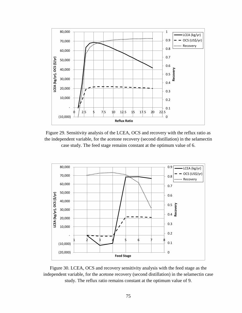
75

Figure 29. Sensitivity analysis of the LCEA, OCS and recovery with the reflux ratio as

the independent variable, for the acetone recovery (second distillation) in the selamectin

case study. The feed stage remains constant at the optimum value of 6.

Figure 30. LCEA, OCS and recovery sensitivity analysis with the feed stage as the

independent variable, for the acetone recovery (second distillation) in the selamectin case

study. The reflux ratio remains constant at the optimum value of 9.

0

0.1

0.2

0.3

0.4

0.5

0.6

0.7

0.8

0.9

1

(10,000)

-

10,000

20,000

30,000

40,000

50,000

60,000

70,000

80,000

0 2.5 5 7.5 10 12.5 15 17.5 20 22.5

Rec

ove

ry

LCEA

(kg

/yr)

, OC

S ($

/yr)

Reflux Ratio

LCEA (kg/yr)

OCS (US$/yr)

Recovery

0

0.1

0.2

0.3

0.4

0.5

0.6

0.7

0.8

0.9

(20,000)

(10,000)

-

10,000

20,000

30,000

40,000

50,000

60,000

70,000

80,000

1 2 3 4 5 6 7 8

Re

cove

ry

LCEA

(kg

/yr)

, OC

S ($

/yr)

Feed Stage

LCEA (kg/yr)

OCS (US$/yr)

Recovery

76

The nelfinavir case RRSA (Figure 31) shows a maximum LCEA at a reflux ratio

of 14 and a maximum OCS at a reflux ratio of 28. As in the selamectin case, both LCEA

and OCS are positive at either maximum. At the LCEA optimum reflux ratio, the OCS

are 98.8 % that of the maximum OCS. The optimum feed stage, for both OCS and LCEA,

as 5. At the LCEA optimum reflux ratio, the purchase of virgin IPA for the process is

reduced from 67,700 kg/yr to 6,400 kg/yr, being the IPA recovery 90.5 %.

Figure 31. LCEA, OCS and recovery sensitivity analysis with the reflux ratio as the

independent variable, for the nelfinavir case study. The feed stage remains constant at the

optimum value of 5.

0

0.1

0.2

0.3

0.4

0.5

0.6

0.7

0.8

0.9

1

-

50,000

100,000

150,000

200,000

250,000

300,000

2 4 6 8 10 12 14 16 18 20 22 24 26 28

Rec

ove

ry

LCEA

(kg

/yr)

, OC

S ($

/yr)

Reflux Ratio

LCEA (kg/yr)

OCS (US$/yr)

Recovery

77

Figure 32. Sensitivity analysis of the LCEA, OCS and recovery with the feed stage as the

independent variable, for the nelfinavir case study. The reflux ratio remains constant at

the optimum value of 14.

The hydrocortisone case RRSA is shown in Figure 33. This graph shows that both

LCEA and OCS curves have a spike at a reflux ratio of 5. The spike occurs because

secondary component, acetone, is also being recovered. Below a reflux ratio of 5, the

system only targets toluene recovery, but at a reflux ratio of 5 and above, the mass

composition of acetone in the distillate is equal or higher than the acetone required purity,

justifying its recovery as well. The feed stage sensitivity analysis of this case (Figure 34)

shows also a spike, for the same reason, at a feed stage of 5. Although in both sensitivity

analyses, the OCS spike looks smaller than the LCEA one, it represents a 24,500 US$/yr

increase. In this case, a 100 % recovery is achieved, since both the distillate (acetone) and

the bottoms (toluene) streams are recovered. The feed stage sensitivity analysis also

shows a spike at a feed stage of 6. From feed stages 2 to 5, only toluene is recovered,

0.82

0.84

0.86

0.88

0.9

0.92

0.94

0.96

0.98

1

-

50,000

100,000

150,000

200,000

250,000

300,000

1 2 3 4 5 6 7 8

Rec

ove

ry

LCEA

(kg

/yr)

, OC

S ($

/yr)

Feed Stage

LCEA (kg/yr)

OCS (US$/yr)

Recovery

78

while at a feed stage of 6 and 7, acetone can be recovered as well. In this case the

emissions in the recovery process are only the ones from the steam and electricity needed

to run the distillation column, since both solvents are recovered and their manufacture

and incineration avoided.

Figure 33. Sensitivity analysis of the LCEA, OCS and recovery with the reflux ratio as

the independent variable, for the hydrocortisone case study. The feed stage remains

constant at the optimum value of 6.

0.86

0.88

0.9

0.92

0.94

0.96

0.98

1

-

200,000

400,000

600,000

800,000

1,000,000

1,200,000

1,400,000

0 2.5 5 7.5 10 12.5 15 17.5 20 22.5R

eco

very

LCEA

(kg

/yr)

, OC

S ($

/yr)

Reflux Ratio

LCEA (kg/yr)

OCS ($/yr)

Recovery

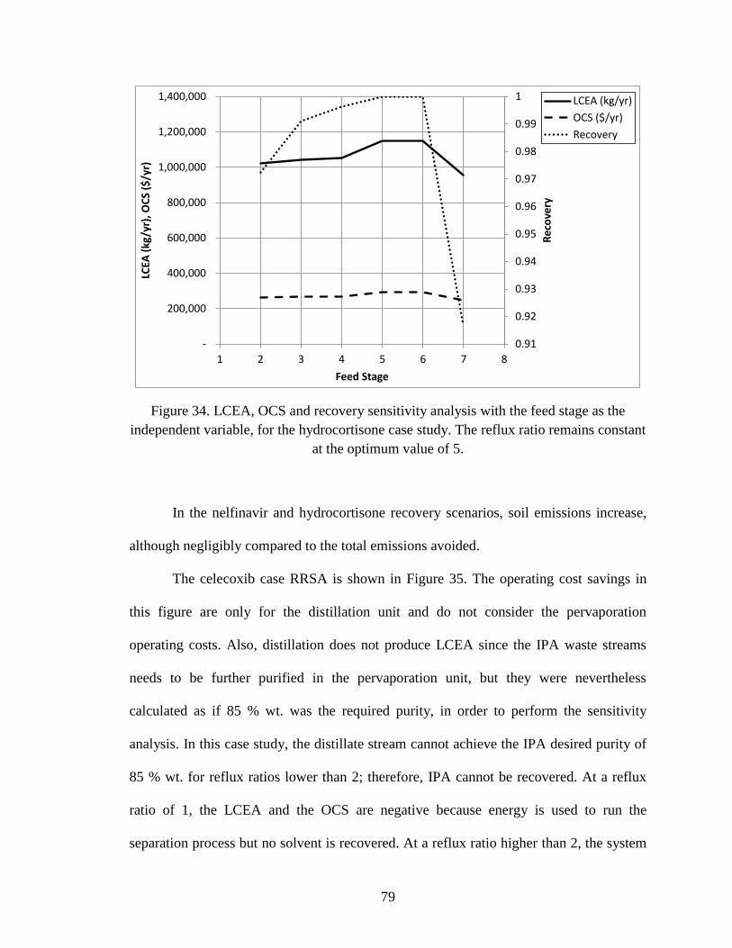
79

Figure 34. LCEA, OCS and recovery sensitivity analysis with the feed stage as the

independent variable, for the hydrocortisone case study. The reflux ratio remains constant

at the optimum value of 5.

In the nelfinavir and hydrocortisone recovery scenarios, soil emissions increase,

although negligibly compared to the total emissions avoided.

The celecoxib case RRSA is shown in Figure 35. The operating cost savings in

this figure are only for the distillation unit and do not consider the pervaporation

operating costs. Also, distillation does not produce LCEA since the IPA waste streams

needs to be further purified in the pervaporation unit, but they were nevertheless

calculated as if 85 % wt. was the required purity, in order to perform the sensitivity

analysis. In this case study, the distillate stream cannot achieve the IPA desired purity of

85 % wt. for reflux ratios lower than 2; therefore, IPA cannot be recovered. At a reflux

ratio of 1, the LCEA and the OCS are negative because energy is used to run the

separation process but no solvent is recovered. At a reflux ratio higher than 2, the system

0.91

0.92

0.93

0.94

0.95

0.96

0.97

0.98

0.99

1

-

200,000

400,000

600,000

800,000

1,000,000

1,200,000

1,400,000

1 2 3 4 5 6 7 8

Rec

ove

ry

LCEA

(kg

/yr)

, OC

S ($

/yr)

Feed Stage

LCEA (kg/yr)

OCS ($/yr)

Recovery

80

is able to recover IPA at a mass composition equal to its required purity. The optimum

reflux ratio in this case study is approximately 2 for both the LCEA and OCS. The feed

stage sensitivity analysis of this case (Figure 36) shows the same behavior: at a feed stage

lower than 6, the LCEA and OCS are negative because IPA is not recovered, while

energy is utilized.

In the celecoxib case, 2,548,407 kg/yr of IPA are avoided to manufacture,

representing a recovery rate of 99.5%. This case study demonstrates that the recovery of

solvents from more difficult to separate azeotropic mixtures can still achieve carbon

footprint reductions and operating cost savings.

Figure 35. Sensitivity analysis of the LCEA, OCS and recovery with the reflux ratio as

the independent variable, for the celecoxib case study. The feed stage remains constant at

the optimum value of 6.

0

0.1

0.2

0.3

0.4

0.5

0.6

0.7

0.8

0.9

1

(4,000,000)

(2,000,000)

-

2,000,000

4,000,000

6,000,000

8,000,000

10,000,000

12,000,000

14,000,000

0 2 4 6 8 10 12 14 16 18 20 22

Rec

ove

ry

LCEA

(kg

/yr)

, OC

S ($

/yr)

Reflux Ratio

LCEA (kg/yr)

OCS ($/yr)

Recovery

81

Figure 36. Sensitivity analysis of the LCEA, OCS and recovery with the feed stage as the

independent variable, for the celecoxib case study. The reflux ratio remains constant at

the optimum value of 2.

The selection of the optimum feed stage determined by our tool can also provide

significant emissions and cost savings, as seen in Figure 27, Figure 32, Figure 34, and

Figure 36. The feed stage sensitivity analysis would not be useful when rating an existing

column that already has a feed plate that cannot be rearranged. In this case, the feed stage

sensitivity analysis should be run with the existing feed stage as a constant. It may occur,

however, that a distillation column has more than one feed location from which to

choose. In this case, our tool can run sensitivity analyses with these existing feed

locations as the independent variables to obtain the optimum available feed location. In

our recovery skid, we have imagined that the distillation column has multiple feed stages

and that the internals can be rearranged to modify the feed stage.

0

0.1

0.2

0.3

0.4

0.5

0.6

0.7

0.8

0.9

1

(4,000,000)

(2,000,000)

-

2,000,000

4,000,000

6,000,000

8,000,000

10,000,000

12,000,000

14,000,000

1 2 3 4 5 6 7 8

Rec

ove

ry

LCEA

(kg

/yr)

, OC

S ($

/yr)

Feed Stage

LCEA (kg/yr)

OCS ($/yr)

Recovery

82

A comparison between the life cycle emissions of the base case and the recovery

case, for each case study is shown from Figure 37 to Figure 40. A small increase in the

recovery process emissions generates significant life cycle emissions reduction.

Conversely, small recovery process costs generate significant monetary savings in the

purchase of virgin solvents and waste treatment (i.e.: incineration) of solvent waste, as

shown in Figure 41 through Figure 44. In the hydrocortisone case study, life cycle

emissions and operating costs in the recovery case are zero because both solvents

(acetone and toluene) are recovered. In the celecoxib case study, the raw materials life

cycle emissions and operating costs in the recovery case are negligible because the

remaining component in the solvent waste is water, which has very little cost and low life

cycle emissions.

Figure 37. Life cycle emissions comparison between base case and recovery case in the

selamectin case study.

0

50,000

100,000

150,000

200,000

250,000

300,000

350,000

400,000

Base Case Recovery Case

Life

Cyc

le E

mis

sio

ns

(kg/

yr) Recovery Process

Incineration

Raw Materials

83

Figure 38. Life cycle emissions comparison between base case and recovery case in the

nelfinavir case study.

Figure 39. Life cycle emissions comparison between base case and recovery case in the

hydrocortisone case study.

0

50,000

100,000

150,000

200,000

250,000

300,000

350,000

400,000

450,000

Base Case Recovery Case

Life

Cyc

le E

mis

sio

ns

(kg/

yr)

Recovery Process

Incineration

Raw Materials

0

200,000

400,000

600,000

800,000

1,000,000

1,200,000

1,400,000

Base Case Recovery Case

Life

Cyc

le E

mis

sio

ns

(kg/

yr)

Recovery Process

Incineration

Raw Materials

84

Figure 40. Life cycle emissions comparison between base case and recovery case in the

celecoxib case study.

Figure 41. Operating costs comparison between base case and recovery case in the

selamectin case study.

0

5,000,000

10,000,000

15,000,000

20,000,000

25,000,000

Base Case Recovery Case

Life

Cyc

le E

mis

sio

ns

(kg/

yr)

Recovery Process

Incineration

Raw Materials

0

50,000

100,000

150,000

200,000

250,000

300,000

350,000

Base Case Recovery Case

Op

erat

ing

Co

sts

(US$

/yr)

Recovery Process

Incineration

Raw Materials

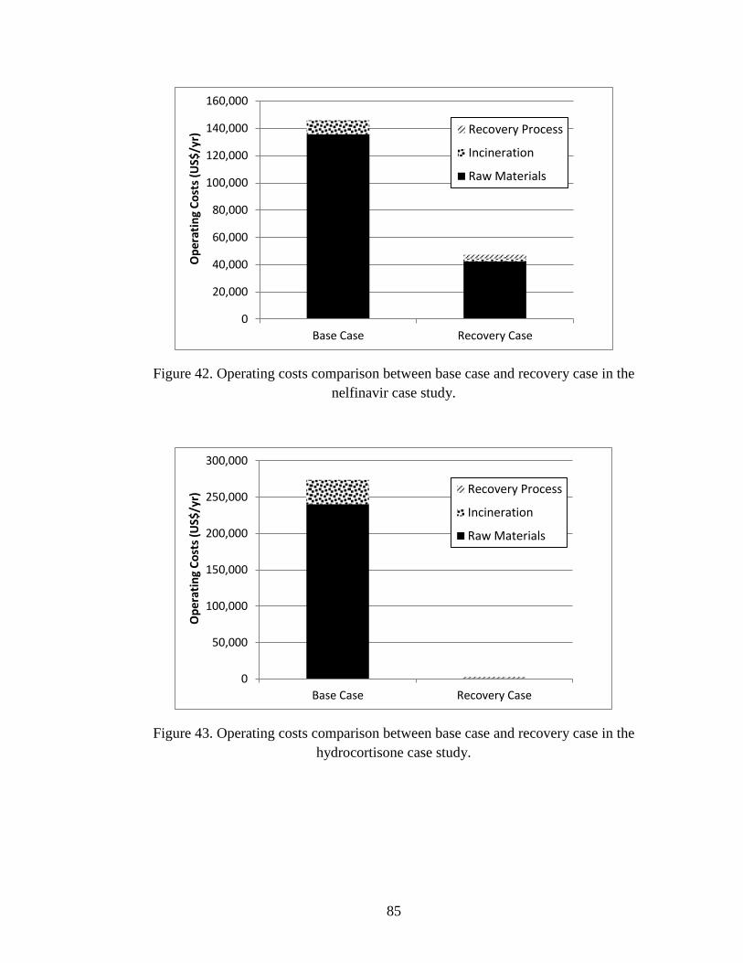
85

Figure 42. Operating costs comparison between base case and recovery case in the

nelfinavir case study.

Figure 43. Operating costs comparison between base case and recovery case in the

hydrocortisone case study.

0

20,000

40,000

60,000

80,000

100,000

120,000

140,000

160,000

Base Case Recovery Case

Op

erat

ing

Co

sts

(US$

/yr)

Recovery Process

Incineration

Raw Materials

0

50,000

100,000

150,000

200,000

250,000

300,000

Base Case Recovery Case

Op

erat

ing

Co

sts

(US$

/yr)

Recovery Process

Incineration

Raw Materials

86

Figure 44. Operating costs comparison between base case and recovery case in the

celecoxib case study.

The IRR for all case studies but nelfinavir’s are positive. The skid could be used

to recover all four solvent waste streams provided proper scheduling, since the

summation of the recoveries operating time, shown in Table 15, is 228 days, i.e., less

than one year. A cash flow analysis for this situation includes the cost savings of the four

recovery projects and the investment cost of one skid, making the economic analysis

results even more attractive. In cases where separation equipment already exist and

remains idle during certain period of time, the investment cost could be smaller or zero,

making the recovery projects more profitable. The selamectin, nelfinavir, and

hydrocortisone processes occur at the same manufacturing plant; therefore, a cash flow

analysis considering the investment cost of one distillation system skid and the savings of

the three cases yielded a higher profitability than the individual cases.

Solvent mixture volatilities are also analyzed as they have a direct impact in

utility consumption. Greenness scoring methods for organic solvents exist that use the

0

1,000,000

2,000,000

3,000,000

4,000,000

5,000,000

6,000,000

Base Case Recovery Case

Op

erat

ing

Co

sts

(US$

/yr)

Recovery Process

Incineration

Raw Materials

87

vapor pressure to determine how easily a solvent mixture can be separated2. However,

relative volatility information alone does not suffice to analyze the complexity of a

mixture separation. Therefore, the Recovery Process Selection Guide can be used as a

screening tool to select solvents for API manufacturing that are easier to separate, making

the process greener. As an example, the company PennAKem®

proposes 2-MeTHF as a

green replacement for THF since it is more easily separated from water because it forms

a heterogeneous mixture, as opposed to the homogeneous and azeotropic mixture formed

by THF and water79

. An evaluation of 2-MeTHF as a green solvent is further presented in

Chapter 6. Equation 3 shows that the higher the LCI of the organic solvent being

recovered, the higher the environmental positive impact of the recovery will be.

Therefore, solvents with high LCI should be prioritized to recover or to be replaced with

green solvents with low LCI.

Conventional vs. R.SWEET’s Optimum Reflux Ratio

Chemical engineering handbooks recommend an economic optimum reflux ratio

between 1.1 and 1.5 times the minimum reflux ratio (Rm). At this range, the combined

capital cost and operating cost is minimized80,81

, as seen in Figure 45. R.SWEET’s

optimum reflux ratios of the selamectin and hydrocortisone cases are significantly higher

than what these conventional values recommend. In more agreement with R.SWEET’s

results, McCormick et al.82

suggest that the minimum reflux ratio multiplier may be 10 or

more, depending on the system and equipment. Very small refluxes, close to the

minimum reflux ratio, may prevent packed towers from being thoroughly wetted; an

undesired situation. McCabe et al.83

explains that most plants are operated at reflux ratios

88

somewhat above the conventional optimum, because the total costs (fixed costs +

operating costs) are not very sensitive to the reflux ratio at a range close to the optimum

(although the upper limit of this range are not specified) and better operating flexibility

can be obtained with reflux ratios greater than the optimum.

The minimum reflux ratio concept is used when the separation between two

components is specified and the number of stages is not specified, since the reflux ratio

defines the number of stages. As the reflux ratio increases, the operating costs increase

due to higher heat duties in the reboiler and condenser, but the number of required

theoretical stages decreases, lowering the height if the column and consequently the fixed

costs. A compromise situation must be met, as shown in Figure 45. The fixed costs reach

a minimum until higher reflux ratios demand for higher column diameters, and they

increase again.

In our situation, the number of stages (or packing height) and column diameter is

already defined. A change in the reflux ratio does not modify the column dimensions.

The minimum reflux design approach is not useful in our case because the recovery skid

has to be flexible to deal with different solvent waste streams, as opposed to a specific

stream. However, to operate the distillation column of the skid one might be tempted to

select the conventional optimum reflux ratio and bypass a deeper analysis, since this may

be time consuming. The minimum reflux ratio could be calculated with the desired

separation specifications. In our case, where the column dimensions are defined, when

the reflux ratio is modified the feed flow could be adjusted to avoid flooding point and

ensure proper mass transfer. Therefore, it is important to highlight that R.SWEET’s

89

optimum reflux ratios do not follow conventional rules of thumb, but an optimum

operation can be achieved without compromising hydraulics performance.

However, R.SWEET model has its limitations, which are explained next. In

R.SWEET's model, increasing the reflux ratio increases the cost of steam and electricity

(to pump more cooling media), but not the cost of the skid. Therefore, it is assumed that

the size of the reboiler and condenser is fixed and can handle the variations in heat duties

that increasing the reflux ratio demands; or that the reboiler and condenser size does not

affect significantly the skid cost. In other words, the cost of the skid doesn't change with

the reflux ratio variation. In R.SWEET model, the demand for greater heat duties when

increasing the reflux ratio is satisfied with an increase in the cooling media and steam

flow rates in the condenser and reboiler, respectively. This higher flow rates increase the

cost of steam and electricity, used for pumping the cooling media. In reality, a heat duty

increase may require an increase in the condenser or reboiler size, increasing the skid

cost, or by using a higher pressure steam or cooling media with lower inlet temperature.

Therefore, R.SWEET assumes that:

The skid cost increase demanded by the condenser or reboiler size increase is not

significant, and/or

The cost increase of using a different heat transfer medium is not significant.

Note that, in R.SWEET’s model, the distillation column itself does not change its

dimensions, since the feed flow rate is adjusted at R.SWEET's optimum reflux ratio to

avoid flooding.

With these assumptions, solvent recovery analyses can be enriched with an

environmental life cycle and economic approach to provide not only green engineering,

90

but smart engineering as well. R.SWEET analysis can be applied to existing distillation

columns or to the design of flexible solvent recovery skids. In R.SWEET, the results of a

RRSA include the reboiler heat duty, which can be used to limit the reflux ratio increase.

The reflux ratio cannot be higher than that which results in a reboiler and/or condenser

heat duty that exceeds its maximum allowable, whether the reboiler and/or condenser

already exists or are in the design phase.

As shown in Table 16, when using R.SWEET’s optimum reflux ratio, the

emissions and cost savings are as much as 49.7 % and 59.9 % higher, respectively, than if

the traditional optimal values for reflux ratio were used. In the acetonitrile recovery of the

selamectin case, the reflux ratio that maximized the LCEA was considered the optimum,

because the reflux ratio that maximized the OCS was 28, which seems impractical, and

because the reflux ratio that maximizes LCEA generates OCS that are 95.1% the

maximum OCS. The conventional optimum reflux ratio for the acetone recovery in the

selamectin case study did not achieve the desired purity of acetone, and therefore it was

not considered in this analysis.

The ability to determine an optimum reflux ratio is a key advantage to operators

and engineers that use R.SWEET. In the nelfinavir and celecoxib cases, the Underwood

minimum reflux ratio was not calculated because both IPA and THF, and IPA and water

mixture are strongly non ideal, in which the Underwood equation is not applied. The IPA

and THF mixture shows a tangent pinch, as shown in Figure 18, while the IPA and water

mixture contains an azeotrope. On the contrary, the acetone and acetonitrile mixture

(selamectin case), and toluene and acetone mixture (hydrocortisone case), show ideal

91

thermodynamic behavior, as seen in Figure 15 and Figure 21, respectively. A detailed

calculation of the Underwood minimum reflux ratio is provided in Appendix K.

Figure 45. Conventional optimum reflux ratio analysis. Adapted from Seader et al

(1997)80

.

Table 16. LCEA and OCS obtained with our tools optimum reflux ratio and with

conventional optimum reflux ratio

Case Study Selamectin -

Acetonitrile Recovery Hydrocortisone

LCEA

(kg/yr)

with conventional optimum

reflux ratio 123,301 946,587

with R.SWEET’s OCS optimum

reflux ratio 184,635 1,148,713

Improvement (%) 49.7 21.4

OCS

(US$/yr)

with conventional optimum

reflux ratio 134,529 241,598

with R.SWEET’s OCS optimum

reflux ratio 215,139 293,286

Improvement (%) 59.9 21.4

An

nu

al C

ost

($

)/ye

ar

Reflux Ratio

Total Cost

Operating Cost

Capital Cost

Rmin Ropt

Optimum Reflux Ratio

92

Pervaporation Membranes Comparison with R.SWEET

In the celecoxib case, the performance of two polymeric membranes, PERVAP®

2510 and PERVAP®

2201 from Sulzer Chemtech, and a ceramic membrane from Mitsui

& Co. were compared using the PV Simulator. The results show that membrane

PERVAP®

2201 could not be used for the celecoxib case, since its minimum required

area (245 m2) is higher than the available area (210 m

2). The Mitsui membrane showed

very promising results, requiring the lowest membrane area of 50 m2. However, the

pervaporation unit design was based on Sulzer’s flat sheet membranes, so Mitsui tubular

membranes would have been incompatible with the skid; therefore, only Sulzer’s

membranes were considered. The PERVAP®

2510 showed that it can achieve the desired

recovery in the celecoxib case in a continuous mode combined with distillation.

Furthermore, its feed and inter-module heater outlet temperature could be reduced to 84

°C, from the original estimate of 95 °C, while still using the available membrane area of

210 m2 and achieving the desired separation, which would reduce the heat requirements

by 10.6 %. These results aided in the pervaporation membrane selection for the skid. This

analysis shows that the PV simulator can be used to easily assess the performance of

different type of membranes for a given recovery project. The experimental data to model

these membranes were obtained from Qiao et al.54

and Van Hoof, et al.35

.

93

Chapter 5

A Heterogeneous Case

To show how R.SWEET is used to separate heterogeneous mixtures, a

hypothetical case study was analyzed. The selected waste was a mixture of methyl ethyl

ketone (MEK) and water, with equal mass composition. The target solvent was MEK at a

mass composition of 99 wt. %. A waste mass of 100,000 kg per year was assumed. The

RPSG tells us that this mixture is heterogeneous at this composition and at 25 °C. The

MEK composition in the heavy phase is 12 wt. %, while the light phase contains 93 wt.

%. Furthermore, an azeotrope is present at a composition of 87.5 wt. %, with a boiling

point of 73.5 °C. Figure 46, shows how this information is presented by the RPSG. At the

bottom of Figure 46, the recommended process can also be seen.

Figure 46. Information output of the RPSG for the hypothetical case study of MEK and

water.

94

R.SWEET uses this information to simulate the distillation of the light phase, in

which MEK is recovered in the bottoms at 99 wt. %, since its boiling point is higher than

the azeotrope’s boiling point. The separation process is depicted in Figure 47. To solve

the decanter mass balance, R.SWEET uses the lever rule. A distillation column with the

characteristics of the skid described in Chapter 3 was used.

Figure 47. MEK dehydration process for the heterogeneous case study.

The recovery of the decanter was 87.3 %, and in the distillation 50.2 %, resulting

in an overall recovery of 43.8 %. Even at this relatively low recovery, LCEA and OCS

are obtained. The distillation RRSA (Figure 48) and feed stage sensitivity analysis

(Figure 49) shows that both LCEA and OCS are maximized at a reflux ratio of 2 and feed

stage of 5.

These results could be improved by increasing the recovery. The problem with this

separation is that two streams that contain MEK are not being recovered: the heavy phase

of the decanter, containing 12 wt. % of MEK and the distillate of the distillation, with 88

Waste Mixture:

MEK (50 wt. %)

Water (50 wt. %)

100,000 kg/yr

B

Water (88 wt. %)

53,086 kg/yr

MEK (93 wt. %)

46,914 kg/yr

A: Decanting

B: Distillation

MEK (99 wt. %)

22,137 kg/yr

A

Light Phase

Heavy Phase

Azeotrope

MEK 88 wt. %)

24,777 kg/yr

95

wt. %, which is almost the azeotropic composition. To increase the recovery, there are

two possibilities:

1) to design a process such as shown in Figure 50, or

2) to sequentially use the process in Figure 47 to separate MEK from the both

streams previously mentioned, i.e., to re-introduce the azeotrope from the

distillate to the decanter.

Nevertheless, these options may not always be possible to implement due to equipment

availability. It is interesting to note, however, that a simple scheme (Figure 47) showed

promising results.

Currently, R.SWEET does not contain the degree of process ramification required

to recommend a wide variety of separation process from which to select, which could

result, for example, in the Figure 50 process. Further programming would be required.

96

Figure 48. Sensitivity analysis of the LCEA, OCS with the reflux ratio as the independent

variable, for the heterogeneous case study. The feed stage remains constant at the

optimum value of 5.

Figure 49. Sensitivity analysis of the LCEA, OCS with the feed stage as the independent

variable, for the heterogeneous case study. The reflux ratio remains constant at the

optimum value of 2.

-

20,000

40,000

60,000

80,000

100,000

120,000

140,000

160,000

180,000

0 1 2 3 4 5 6 7

LCEA

(kg

/yr)

, OC

S ($

/yr)

Reflux Ratio

LCEA (kg/yr)

OCS (US$/yr)

-

20,000

40,000

60,000

80,000

100,000

120,000

140,000

160,000

180,000

1 2 3 4 5 6 7 8

LCEA

(kg

/yr)

, OC

S ($

/yr)

Feed Stage

LCEA (kg/yr)

OCS (US$/yr)

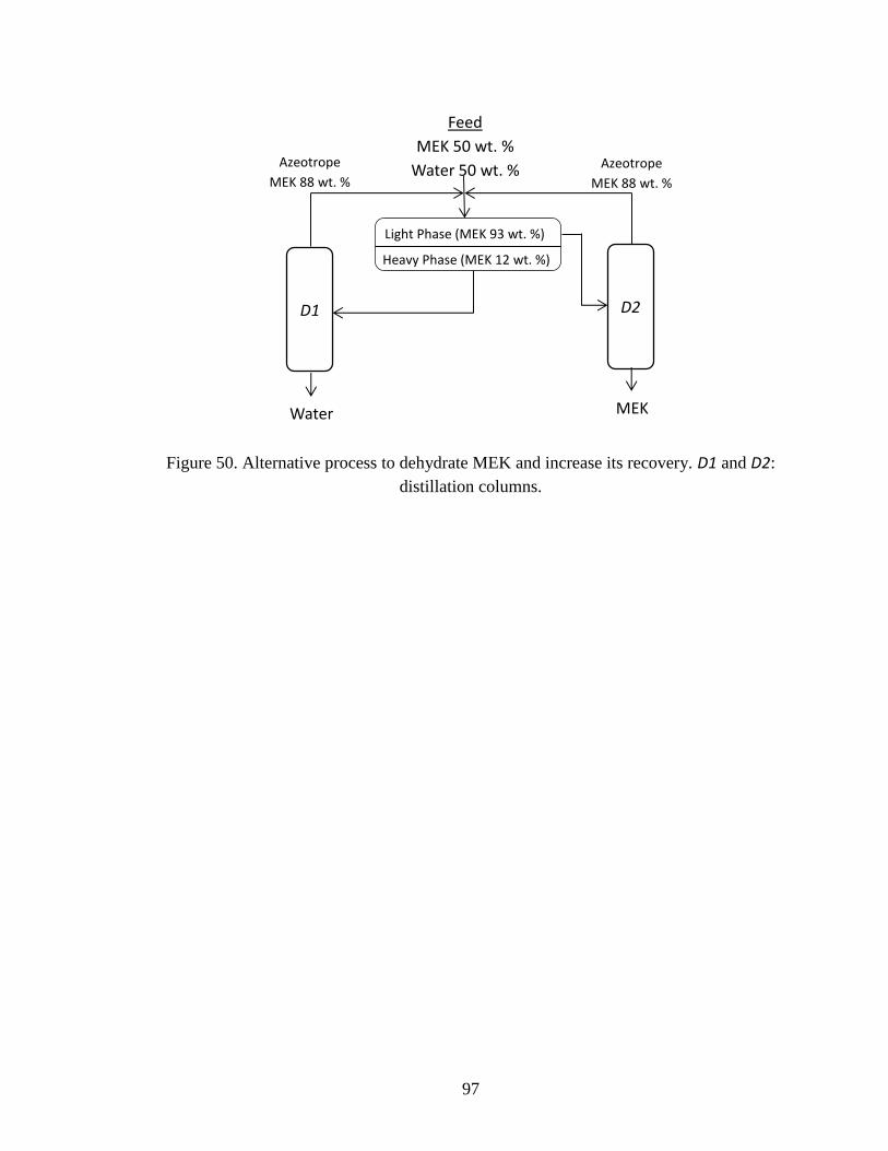
97

Figure 50. Alternative process to dehydrate MEK and increase its recovery. D1 and D2:

distillation columns.

Feed

MEK 50 wt. %

Water 50 wt. %

Light Phase (MEK 93 wt. %)

D2D1

Water MEK

Azeotrope

MEK 88 wt. %

Azeotrope

MEK 88 wt. %

Heavy Phase (MEK 12 wt. %)

98

Chapter 6

Green Solvents

Another way of reducing the environmental impact of organic solvent use in the

pharmaceutical industry is by using green solvents. Green solvent may have one or more

of these characteristics, as compared to conventional solvent: 1) lower LCI, 2) lower

toxicity and 3) easily recovered for recycle. Organic solvents with lower LCI are usually

derived from renewable sources such as bio-waste or agricultural by-products. The

second characteristic is usually associated with low volatility, resulting in a less

probability to be inhaled by humans, creating thus a safer work environment, or to be

released to the environment due to fugitive emissions. The ability to form biphasic

systems is an attractive property of organic solvents because it allows for less energy

intensive and more efficient separation and recovery10

. These characteristics are present

in 2-methyl tetrahydrofuran (MeTHF), produced by PennAKem and marketed as

ecoMeTHFTM

.

MeTHF is produced by PennAKem and sold as a potential replacement for THF,

which is widely used in pharmaceutical syntheses. The use of MeTHF as a solvent in the

pharmaceutical industry has increased steadily from 2005 to 2008 and is expected to keep

increasing. In 2010, the global demand of THF was 525 million kg per year84

and it is

expected to exceed 800 million kg per year in 201785

. PennAKem markets MeTHF as

one of their carbon neutral solvents. This is claimed because the starting material,

furfural, is produced from agricultural by-products. Therefore, PennAKem calls its

product ecoMeTHFTM

. This method of furfural production does not impact the world’s

99

food supply and also keeps PennAKem’s material supply and prices from fluctuating as

highly as they would with a petroleum based chemical. PennAKem claims that

ecoMeTHFTM

is a better solvent choice than THF because it can be recovered from water

more easily, leading to lower costs in both utility and solvent purchasing for the

consumer. Several pharmaceutical companies have already expressed interest in pursuing

this chemical as an alternative to THF.

MeTHF has some unique properties that make it a green solvent. In solvent

polarity and Lewis base strength, MeTHF is between THF and diethyl ether. It is also

useful as a solvent in low-temperature lithiation, lithium aluminum hydride reductions,

metal catalyzed coupling reaction, and the Reformatsky reaction. It can also replace

dichloromethane in biphasic reaction. Due to its low solubility in water at high

temperatures, 6.6% at 60°C, it is easier to separate it from water, as compared to THF.86

THF is miscible in water and forms an azeotrope at atmospheric pressure at a mole

fraction of 0.78. MeTHF forms an azeotrope at atmospheric pressure at a mole fraction of

0.88. A Txy vapor-liquid-liquid and xy vapor-liquid equilibrium curve of MeTHF and

water is shown in Figure 52. NRTL binary interaction coefficients for MeTHF and water

were provided by PennAKem, in order to obtain in Aspen Plus® the previously

mentioned curves.

Aycock proposes that MeTHF can be dehydrated by a decanter followed by batch

distillation with an overhead liquid-liquid phase separator operated at 60°C. The MeTHF

from the separator is refluxed into the column to increase the mass fraction beyond that

of the azeotrope. Dry MeTHF is recovered from the reboiler. The overhead separator is

operated at 60°C because MeTHF is 6.6% soluble in water, but water is only 4.6%

100

soluble in MeTHF86

. This recovery process can serve as the basis for a continuous

distillation solvent recovery simulation. The process scheme used to recover MeTHF and

THF from aqueous waste mixtures was analyzed to evaluate the “greenness” of MeTHF.

The objective of this section is to analyze the environmental impact of

ecoMeTHFTM

versus THF in the production and use in the pharmaceutical industry. In

order to do this, the LCI of ecoMeTHFTM

and THF were generated and the recovery

process for both solvents was modeled. The “chemical” route (conversion of 1,4-

butanediol to THF) and the “biomass” route (conversion of corn to furfural to THF) were

analyzed for the production of THF. In the latter case, the product will be called

ecoTHFTM

. The biogenic carbon approach (BCA) was used when calculating the LCI of

MeTHF and ecoTHFTM

. This approach considers that CO2 emissions are zero when they

are generated from biomass (e.g., incineration of biomass) because the released CO2

originally came from the atmosphere.

MeTHF has the potential to be substituted for THF in organometallic reaction

steps in various API syntheses. Companies Pfizer and Johnson & Johnson has indicated

that they would likely use MeTHF in a replacement ratio of 1:187,88

. This means that for

every kg of THF used, 1 kg of MeTHF could be potentially used as substitute.

The base case corresponds to a waste stream containing a 50-50 % wt. mixture of

chemical THF and water, and the incineration of this waste for energy recovery. This

base case was compared with more environmentally favorable cases involving THF

replacement and waste recovery techniques:

1) the substitution of chemical THF with ecoTHFTM

and the recovery and re-use of

ecoTHFTM

with extractive distillation, using glycol as entrainer;

101

2) the substitution of chemical THF with ecoTHFTM

and the recovery and re-use of

ecoTHFTM

with continuous distillation followed by pervaporation; and

3) the substitution of chemical THF with ecoMeTHFTM

, and the recovery of the

ecoMeTHFTM

waste with a decanter-distillation system.

The comparison of the two ecoTHFTM

recovery processes had the additional objective

of analyzing the greenness of pervaporation89

.

Figure 51. MeTHF and water vapor-liquid equilibrium. An azeotrope occurs at a mole

fraction of 0.88 at atmospheric pressure.

0

0.1

0.2

0.3

0.4

0.5

0.6

0.7

0.8

0.9

1

0 0.1 0.2 0.3 0.4 0.5 0.6 0.7 0.8 0.9 1

MeT

HF

vap

or

mo

le f

ract

ion

(y)

MeTHF Mole Fraction in Liquid (x)

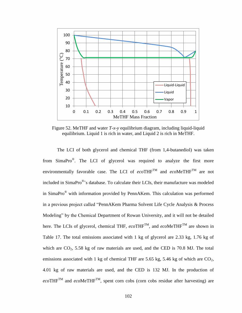
102

Figure 52. MeTHF and water T-x-y equilibrium diagram, including liquid-liquid

equilibrium. Liquid 1 is rich in water, and Liquid 2 is rich in MeTHF.

The LCI of both glycerol and chemical THF (from 1,4-butanediol) was taken

from SimaPro®

. The LCI of glycerol was required to analyze the first more

environmentally favorable case. The LCI of ecoTHFTM

and ecoMeTHFTM

are not

included in SimaPro®’s database. To calculate their LCIs, their manufacture was modeled

in SimaPro®

with information provided by PennAKem. This calculation was performed

in a previous project called “PennAKem Pharma Solvent Life Cycle Analysis & Process

Modeling” by the Chemical Department of Rowan University, and it will not be detailed

here. The LCIs of glycerol, chemical THF, ecoTHFTM

, and ecoMeTHFTM

are shown in

Table 17. The total emissions associated with 1 kg of glycerol are 2.33 kg, 1.76 kg of

which are CO2, 5.58 kg of raw materials are used, and the CED is 70.8 MJ. The total

emissions associated with 1 kg of chemical THF are 5.65 kg, 5.46 kg of which are CO2,

4.01 kg of raw materials are used, and the CED is 132 MJ. In the production of

ecoTHFTM

and ecoMeTHFTM

, spent corn cobs (corn cobs residue after harvesting) are

10

20

30

40

50

60

70

80

90

100

0 0.1 0.2 0.3 0.4 0.5 0.6 0.7 0.8 0.9 1

Tem

per

ature

( C

)

MeTHF Mass Fraction

Liquid-Liquid

Liquid

Vapor

103

used to make furfural, which is then used to create furan to produce ecoTHFTM

, and

methyl furan to produce ecoMeTHFTM

.

Table 17. LCI from SimaPro®

for 1kg of Glycerol, 1 kg of chemical THF, 1 kg of

ecoTHFTM

and 1 kg of ecoMeTHFTM

THF

Manufacture

Glycerol

Manufacture

ecoTHFTM

ecoMeTHFTM

Total Raw Materials

Used, kg 4.01E+00 5.58E+00 5.33E+02 1.21E+02

Total CED, MJ-Eq 1.28E+02 7.08E+01 6.15E+00 -2.00E+01

Total Air Emissions, kg 5.52E+00 1.79E+00 1.45E+00 1.62E-01

CO2, kg 5.46E+00 1.76E+00 1.39E+00 1.50E-01

CO, kg 4.82E-03 1.14E-02 7.32E-03 6.63E-03

Methane, kg 1.45E-02 4.46E-03 2.72E-03 -9.38E-04

NOX, kg 8.67E-03 4.79E-03 3.26E-02 1.38E-02

NMVOC, kg 3.25E-03 8.03E-04 2.94E-03 2.46E-03

Particulates, kg 3.57E-03 2.36E-03 9.74E-04 1.26E-03

SO2, kg 1.15E-02 3.91E-03 1.77E-02 -4.55E-03

Total Water Emissions,

kg 1.26E-01 5.34E-01 3.41E-02 2.73E-02

VOCs, kg 7.93E-06 2.73E-06 5.82E-06 5.56E-06

Total Soil Emissions, kg 2.31E-03 1.77E-03 2.08E-03 1.94E-03

Total Emissions, kg 5.65E+00 2.33E+00 1.49E+00 1.91E-01

The production of 1 kg of ecoTHFTM generates 1.49 kg of emissions, most of

which are released to the air. The CO2 emissions are 1.39 kg, and the CED is 6.15 MJ-

Eq/kg. The production of ecoMeTHFTM

generates 0.191 kg of total life cycle emissions

per kg of ecoMeTHFTM

produced. A total of 0.162 kg of air emissions, including 0.150

kg of CO2, are created in the production of ecoMeTHFTM

. The process also avoids 20 MJ-

Eq/kg of CED. The production of ecoMeTHFTM

is greener than both chemical THF and

ecoTHFTM

. Manufacturing 1 kg of ecoMeTHFTM

instead of 1 kg of THF would reduce

104

5.46 kg of emissions (97 % reduction), while the manufacture of ecoTHFTM

would avoid

4.16 kg of emissions (74 % reduction). This information is useful to the pharmaceutical

sector in guiding decision makers with solvent substitution strategies for greener API

syntheses. Therefore, ecoMeTHFTM

has the potential to make a significant impact on the

sustainability of the pharmaceutical and fine chemical sector. However, this provides

only a cradle to gate analysis because the disposal of the solvent is not being considered.

In a cradle to grave LCA, the LC emissions of the recovery need to be calculated

as well. The boundaries for this analysis include solvent cradle to solvent grave and

therefore solvent waste recovery is evaluated. The objective is to answer: which is a

better alternative to chemical THF: ecoTHFTM

or ecoMeTHFTM

? The recovery of

ecoTHFTM

and ecoMeTHFTM

from water has an impact in the answer of this question, as

less energetic recoveries are environmentally friendlier. Note that chemical THF and

ecoTHFTM

are the same chemical, but the ecoTHFTM

manufacture process is more

environmentally friendly as ecoTHFTM

is produced from furfural (a bio-based raw

material, manufactured from corn cobs), which is reflected in the LCI difference.

The recovery of ecoTHFTM

from a 50-50 % wt. mixture was modeled as an

extractive distillation process and as a distillation followed by a pervaporation unit. The

dehydration of MeTHF using the same composition was performed with a decantation

followed by two subsequent distillations. The purity specification for both solvents was

assumed to be 99.5 %wt. Aspen Plus®

was utilized to model the separation of the

ecoTHFTM

and water mixture by extractive distillation. Our software tool was used to

simulate the decanting, distillation and pervaporation processes, and to calculate the life

cycle emissions, operating cost savings and cash-flow.

105

The chemical THF incineration LCI is presented in Appendix F. It was assumed

that the fraction of ecoTHFTM

not recovered in both the extractive distillation process and

the distillation and pervaporation process is incinerated. However, its incineration CO2

emissions are zero because ecoTHFTM

is composed of biogenic carbon. The ecoTHFTM

incineration LCI is available in Appendix F. The steam and electricity LCIs used in all

the recovery cases were steam from an average chemical plant and electricity from

United States' production mix, respectively, obtained from SimaPro®

and included in

Appendix G. The reason for this selection is that the facility where the recoveries take

place cannot be specified.

The selection of an entrainer for the dehydration of THF was based upon the

selectivity of the entrainer, the relative volatility change between THF and water, the

miscibility of water and THF, the distillate and residue products, and the azeotrope

formation with the azeotropic THF and water feed. These criteria were studied for five

potential entrainers and the ideal entrainer selected was glycerol. The effect of the five

entrainers of the relative volatility of the mixture can be seen in Figure 53. From this

graph it can be seen that the addition of glycerol increases the relative volatility of THF

and water to the point where the azeotrope no longer exists.

106

Figure 53. Pseudobinary diagram at 30 % entrainer to feed ratio (P = 1 atm), adapted

from Gomez et al.29

An additional consideration is the cost of the entrainer selected. Of the five

potential entrainers, ethylene glycol is cheapest, followed by glycerol. Even though

ethylene glycol has the lowest price and is a suitable candidate, glycerol was chosen

because of the lower toxicity and smaller volumes required29

.

The simulation of the recovery of ecoTHFTM

with glycerol as an entrainer yielded

an ecoTHFTM

recovery of 99.53%. This means that if a pharmaceutical manufacturing

process uses this recovery process, it would need to make up 0.0047 kg of ecoTHFTM

per

kg of ecoTHFTM

used in the process. A mass ratio of 1:1 of glycerol and solvent waste

was used, and the recovery of the glycerol to recycle was 99.95%. Therefore, 0.0010116

kg of glycerol was used per kg of THF fed to the recovery process. The extractive

distillation recovery process diagram can be seen in Figure 54. The steam and electricity

0

0.1

0.2

0.3

0.4

0.5

0.6

0.7

0.8

0.9

1

0 0.1 0.2 0.3 0.4 0.5 0.6 0.7 0.8 0.9 1

TH

F v

apor

mole

fra

ctio

n (

y)

THF Mole Fraction in Liquid (x)

Binary

Butanediol

Hexanediol

Propanediol

Glycerol

107

used per kg of ecoTHFTM

fed to the recovery system was 3.5 kg and 0.52 kWh,

respectively.

Figure 54. Block flow diagram for the extractive distillation of THF from water using

glycerol as an entrainer.

The ecoTHFTM

extractive distillation recovery case life cycle emissions are shown

in Appendix H. A sensitivity analysis was performed to determine the optimal feed stage

and reflux ratio for the two distillation columns given that each column was composed of

8 theoretical trays.

Feed50-50 % wt. THF/Water

Glycerol and Water

THF 99.5 % wt.

Glycerol make-up

Glycerol

Water99.4 % wt.

Entrainer (Glycerol) Recycle

108

Figure 55. Dehydration of THF integrating distillation and pervaporation.

The simulation of the recovery of ecoTHFTM

using distillation and pervaporation

yielded a recovery of 99.25%. The process diagram is shown in Figure 55. The steam and

electricity used per kg of THF used was 0.66 kg and 0.094 kWh, respectively. This

recovery case life cycle emissions are shown in Appendix H. A sensitivity analysis was

used to select the optimum reflux ratio and feed stage for the distillation column, using

R.SWEET. As with the previous cases, a column with 8 theoretical stages was used.

The recovery of ecoMeTHFTM

process diagram is shown Figure 56. The recovery

achieved was 99 %. The reflux ratio and feed stage that maximized the emissions avoided

were selected for both columns. In this case, the theoretical stages for columns # 1 and #

2 were 4 and 5 respectively. The steam and electricity used per kg of ecoMeTHFTM

used

was 0.49 kg and 0.058 kWh, respectively. Comparing these values with those of the THF

recovery, we can see that the energy requirement for the ecoMeTHFTM

recovery is lower.

Feed50-50 % wt. THF/Water

Water

Water

THF 99.5 % wt.

AzeotropeTHF 93 % wt.

Vacuum Pump

109

It was assumed that the fraction of ecoMeTHFTM

not recovered is incinerated. As

with ecoTHFTM

, ecoMeTHFTM

incineration CO2 emissions are zero because it is

composed of biogenic carbon. Since ecoMeTHFTM

is not available in Ecosolvent®

, it was

assumed that the incineration LCI is the same as ecoTHFTM

because both solvents are

chemically similar. The ecoMeTHFTM

recovery case LC emissions are presented in

Appendix H. A comparison between the environmentally favorable cases shows that the

ecoMeTHFTM

case is the greenest alternative. corresponding reductions.

Figure 56. MeTHF recovery process. LS: Light Phase Stream (high concentrations of

MeTHF), HS: Heavy Phase Stream (high concentrations of water)

The emissions in the recovery cases are lower than in the base case because less

solvent is manufactured and incinerated; therefore, the LC emissions associated to this

Water

aqueous phase(heavy phase)MeTHF 10 % wt.

organic phase(light phase)MeTHF 94 % wt.

Decanter

MeTHF99.5 % wt.

Feed50-50 % wt. MeTHF/Water

Recycle

Recycle

110

processes are lower as well. In the ecoMeTHFTM

recovery case, the reduction of both

total and CO2 emissions is 98 %. The results of the total emissions produced in the three

recovery cases analyzed are shown in Figure 57. It can be seen that the emissions are

lower in the ecoMeTHFTM

recovery case. This study verifies that ecoMeTHFTM

is a green

solvent replacement for THF, as suggested by PennAKem. Note that the raw material

emissions are negligible when compared to the recovery process emissions, which

correspond to the steam and electricity emissions. Therefore, this analysis shows that the

steam and electricity use in the ecoMeTHFTM

recovery case is the lowest, which means it

is easier to recover MeTHF than THF, as claimed by PennAKem. This result indicates

that when the recovery is included in the LCA, the higher ease of recovery of MeTHF as

compared to THF has a significant impact in the “greenness” of the API manufacturing.

The total life cycle emissions of the THF use when recovering THF with

distillation followed by pervaporation are 81% lower than when recovering THF with

extractive distillation. This result fulfills the second objective of this chapter, which was

to prove that pervaporation is a greener recovery process than extractive distillation.

111

Figure 57. Total emission generated in the recovery cases

The cost of THF, US$3.28/kg, was obtained through ICIS Pricing21

. The cost of

MeTHF was neither provided nor available at ICIS Pricing. Its bulk price was, however,

estimated with the price of smaller volumes of the same chemical available at the

laboratory providers Spectrum90

and Sigma-Aldrich91

websites. A MeTHF to THF price

ratio (using a price for the same container volume, for comparison consistency) from the

two providers was calculated and averaged. The averaged ratio was then multiplied by

the known THF bulk price. The algebraic expression is as follows:

(

)

The resulting MeTHF price was determined to be US$8.71/kg. The cost of steam,

electricity and waste management was assumed to be the same as in the Kalamazoo plant

in Michigan (Selamectin case), since it is reasonable that this plant is representative of a

0,00E+00

2,00E-01

4,00E-01

6,00E-01

8,00E-01

1,00E+00

1,20E+00

1,40E+00

ecoTHF (Extractive Distillation) ecoTHF (Dist+PV) ecoMeTHF

kg t

ota

l lif

e c

ycle

em

issi

on

s

Recovery

Raw Materials andIncineration

112

typical pharmaceutical plant in the United States. The cost of glycerol, US$2.28/kg, for

the extractive distillation recovery case was also obtained from ICIS Pricing21

. The

incineration cost was assumed to be the same as in the Kalamazoo plant.

The economic analysis of the base case and of the THF and MeTHF recovery

cases is shown in Table 18, Table 19, Table 20 and Table 21. The savings are calculated

as the base case cost minus the recovery case cost.

Table 18. Base case economic analysis

Quantity

(kg/kg THF

use)

Unitary Price

(US$/kg)

Cost

(US$/year)

THF 1 3.28 3.28

Waste Management 1 0.129 0.129

Total = 3.41

Table 19. THF extractive distillation recovery case economic analysis

Quantity

(kg/kg THF use,

*kWh/kg THF use)

Unitary Price

(US$/kg, *US$/kWh)

Cost

(US$/kg

THF use)

THF 0.0047 3.28 0.0154

Glycerol 0.00102 2.28 0.00232

Waste Management 0.0047 0.129 0.000131

Steam 3.46 0.02 0.0692

Electricity* 0.521 0.1 0.0521

Total = 0.124

Savings = 3.29

113

Table 20. THF distillation + pervaporation recovery case economic analysis

Quantity

(kg/kg THF use,

*kWh/kg THF use)

Unitary Price

(US$/kg, *US$/kWh)

Cost

(US$/kg

THF use)

THF 0.00748 3.28 0.0245

Waste Management 0.00748 0.129 0.000964

Steam 0.660 0.02 0.0132

Electricity* 0.0941 0.1 0.00941

Total = 0.0481

Savings = 3.36

Table 21. MeTHF recovery case economic analysis

Quantity

(kg/kg MeTHF use,

*kWh/kg MeTHF use)

Unitary Price

(US$/kg, *US$/kWh)

Cost

(US$/kg

MeTHF use)

ecoMeTHFTM

Purchase 0.0100 8.71 0.0873

Waste Management 0.0100 0.129 0.00129

Steam 0.49 0.02 0.00974

Electricity* 0.058 0.1 0.00577

Total = 0.104

Savings = 3.31

The economic analysis results show that, even though MeTHF costs more than

twice than THF, the operating costs in the MeTHF recovery case are lower than in the

THF extractive distillation recovery case. This occurs mostly because the quantity of

steam and electricity used in the extractive distillation process are 7 and 9 times,

respectively, the quantities used in the MeTHF case, which reflects the ease of separation

of MeTHF. The THF distillation followed by pervaporation recovery case cost is the

lowest, however, the operating cost savings are almost the same as those of the MeTHF

recovery case, being 98.5 % and 97.1 % of the base case costs, respectively.

114

Chapter 7

Conclusions

An environmental and economic analysis of solvent recovery in the manufacture

of API’s was performed. A software toolbox that combines process simulation with

environmental and economic impact determination was developed. The results of using

our tool in four different solvent waste case studies show that the environmental impact

and the operating cost of API manufacturing can be reduced with solvent recovery.

Our tool was used to determine the near optimum distillation operating parameters that

maximized LCEA and OCS. The reflux ratio sensitivity analysis performed with the tool

showed that conventional heuristics for selecting the optimum reflux ratio do not always

apply to solvent recovery. The tool was also used to aid in the selection of pervaporation

dehydration membranes.

The feasibility of using the same process skid to recover binary solvent mixtures

from LVWS’s and HVWS’s, and with different thermodynamic properties was evaluated

with the R.SWEET tool. All the cases showed positive environmental and economic

results. It was shown that using a single recovery skid to purify solvent waste streams

with different thermodynamic behavior increases the profitability of the recovery project.

The design of a skid flexible enough to treat different waste streams is a key factor to

achieve this profitability.

A “green technology” such as pervaporation was included in the skid to evaluate

its performances and “greenness”. The simulation and economic evaluation results were

satisfactory.

115

The majority of the emissions avoided correspond to the solvent manufacture and

incineration LCE that occur outside the boundaries of the pharmaceutical plant, which is

consistent with results obtained in previous studies and shows the importance of the

LCA. Therefore, green solvents with low LCI should also be used when possible to

reduce the manufacture life cycle emissions. Furthermore, green solvent with easy

recoverability reduce the incineration life cycle emissions.

Currently, the R.SWEET tool has the flexibility to simulate the recovery of

homogeneous azeotropic and non-homogeneous solvent waste mixtures. Future work will

expand the tool capabilities to include

decanting simulation and design;

three-component separation simulation; and

handling of solids.

Although our initial efforts have been focused on the pharmaceutical industry, this

tool has the potential to be applied to other commercial sectors.

Acknowledgments

Support for this project was provided by the United States Environmental

Protection Agency through grant 97212311-0. Special thanks to Rowan students Molly

Russell and Stephen Montgomery, and Pfizer staff Frank Urbanski, Carlos Junco, and

Peter Dunn for their invaluable collaboration.

116

List of References

1 Sheldon, R.A. (1997). Catalysis and pollution prevention. Chem. Ind.,1, 12-15.

2 Slater, C. S., Savelski, M. J., Carole, W. & Constable D. (2010), Solvent Use and Waste Issues. In P.

Dunn, A. Wells, M. Williams (Eds). Green Chemistry in the Pharmaceutical Industry (pp. 2,4, 42-54).

Germany: Wiley-VCH.

3 Jimenez-Gonzalez, C., Ponder, C.S., Broxterman, Q.B. & Manley, J.B. (2011). Using the Right Green

Yardstick: Why Process Mass Intensity is Used in the Pharmaceutical Industry to Drive More Sustainable

Processes. Org. Process Res. Dev.,15, 912–917.

4 Butters, M., Catterick, D., Craig, A., Curzons, A., Dale, D. , Gillmore, A., … White, W. (2006). Critical

Assessment of Pharmaceutical Processes-A Rationale for Changing the Synthetic Route. Chemical

Reviews, 106(7), 3002-27.

5 United States Environmental Protection Agency, Office of Environmental Information, Toxic Release

Inventory Program, TRI-NET (2010) [Database Software]. Retrieved from: http://www2.epa.gov/toxics-

release-inventory-tri-program/download-trinet

6 Slater, C. S. & Savelski, M. J. (2007). A method to characterize the greenness of solvents used in

pharmaceutical industry. Journal in Environmental Science and Health Part A, 42, 1595-1605.

7 United States Environmental Protection Agency (2013, June). Priority Pollutants. Retrieved from

http://water.epa.gov/scitech/methods/cwa/pollutants.cfm/.

8 Verschueren, K. (2001). Handbook of Environmental Data on Organic Chemicals. John Wiley & Sons,

Inc.

9 Montgomery, J.H. (2000). Groundwater Chemicals. Desk Reference (third ed.). Boca Raton, FL, USA:

CRC Press LLC.

10 Clark, J.H. & Tavener, S.J. (2007). Alternative Solvents: Shades of Green. Organic Process Research &

Development, 11, 149-155

11 Boring, A. (2012). Offshoring Production and Intra-industry Trade. ETSG 2012 Leuven, Fourteenth

Annual Conference, 13-15 September 2012. Retrieved from the European Trade Study Group website:

http://www.etsg.org/ETSG2012/Programme/Papers/471.pdf.

12 United States Environmental Protection Agency (2013, September). Solid Waste Management

Hierarchy. Retrieved from the United States Environmental Protection Agency website:

http://www.epa.gov/wastes/nonhaz/municipal/hierarchy.htm

13 Michigan Department of Environmental Quality. Environmental Assistance Division (1998).

Considerations in Selecting a Commercial (Off-Site) Solvent Recycling Service. Fact Sheet.

14 Anastas, P. T. & Zimmerman, J. B. (2003). Design through the Twelve Principles of Green Engineering.

Env. Sci. and Tech., 37(5), 94A-101A.

15 Jimenez-Gonzalez, C., Poechlauer, P., Broxterman, Q. B., Yang, B., Ende, D., Baird, J.,…, Manley, J.

(2011). Key Green Engineering Areas for Sustainable Manufacturing: A Perspective from Pharmaceutical

and Fine Chemicals Manufacturers. Organic Process Research & Development, 15, 900-911.

117

16 United States Environmental Protection Agency (2008). 2009-2014 EPA Strategic Plan Change

Document, Goal 5, Strategic Measure 5.2.1 “Prevent Pollution and Promote Environmental Stewardship”,

Washington, DC.

17 Slater, C.S. & Savelski, M.J. (2009). Towards a Greener Manufacturing Environment. Innovations in

Pharmaceutical Technology, 29, 78-83.

18 Raymond, M. J., Slater, C. S. & Savelski, M. J. (2010). LCA approach to the analysis of solvent waste

issues in the pharmaceutical industry. Green Chem., 12, 1826-1834.

19 ETH Zurich, Safety & Environmental Technology Group (2006). The Ecosolvent Tool (Version 1.0.1)

[Computer Software]. Retrieved from ETH Zurich website: http://www.sust-chem.ethz.ch/tools/ecosolvent/

20 Pre Consultants (2012). SimaPro [Computer LCA Software]. Retrieved from Pre Consultants website:

http://www.pre.nl/simapro/

21 ICIS Pricing (2013, February). Indicative Chemical Prices A-Z. (Editor: Joseph Chang) Retrieved from

ICIS Pricing website http://www.icis.com/chemicals/channel-info-chemicals-a-z/

22 Institute for 21st Century Energy. An Affiliate of the U.S. Chamber of Commerce (2012, May). Crude

oil price volatility. Metric of the month. A deeper look into interesting trends in energy security data.

Retrieved from the Institute for 21st Century Energy website:

http://www.energyxxi.org/sites/default/files/file-tool/MetricoftheMonth-

MAY12CrudeOilPriceVolatility.pdf

23 Rosseau, R. W. (1987). Handbook of Separation Process Technology. Wiley and Sons.

24 The University of Edinburgh, Data Source for Azeotropes. Retrieved from University of Edinburgh

website: http://www.chemeng.ed.ac.uk/people/jack/azeotrope/access.html

25 Felder, R. M. & Rousseau, R. W. (2005), Elementary principles of chemical processes 3rd edition,

Hoboken, NJ: John Wiley & Sons, Inc.

26 Smallwood, I. (2002). Solvent Recovery Handbook (2nd ed., pp. 112). Boca Raton, FL, USA: Blackwell

Science.

27 Geankoplis, C. J. (2003), Transport processes and separation process principles (4th ed.). Upper Saddle

River, NJ, USA: Prentice Hall.

28 Seader, J. D., Henley, E. J. (2006). Separation Process Principles (2nd ed., pp. 12). John Wiley & Sons.

29 Gomez, P. & Gil, I. (2009). Simulation of the Tetrahydrofuran Dehydration Process by Extractive

Distillation in Aspen Plus. Latin American Applied Research, 39, 275-284.

30 Pierotti, G. J. (1948). Extractive Distillation Process. United States Patent 2,455,803.

31 Van Winkle, M. (1968). Distillation. USA: McGraw Hill.

32 Seader, J. D. (2006). Separation Process Principles (2nd. ed., pp 756). NY: John Wiley and Sons.

33 Pham, H. & Doherty, M. (1990). Design and Synthesis of Heterogeneous Azeotropic Distillation II –

Residue Curve Maps. Chemical Engineering Science, 45(7), 1837-1843.

118

34 Bieker, T. & Simmrock, K. H. (1994). Knowledge integrating system for the selection of solvents for

extractive and azeotropic distillation. Computers & Chemical Engineering, 18(Supplement 1), S25-S29.

35 Van Hoof, V., Van den Abeele, L., Buekenhoudt, A., Dotremont, C. & Leysen, R. (2004). Economic

comparison between azeotropic distillation and different hybrid systems combining distillation with

pervaporation for the dehydration of isopropanol. Separation and Purification Technology, 37, 33-49.

36 Slater, C. S., Savelski, M. J., Moroz, T. M. & Raymond, M. J. (2012). Pervaporation as a green drying

process for tetrahydrofuran recovery in pharmaceutical synthesis. Green Chemistry Letters and

Reviews,5(1), 55-64

37 Wynn, N. (2001, October). Pervaporation Comes of Age (October Issue, pp. 66-72). CEP Magazine,

AIChE.

38 Baker, R. W. (2004). Membrane Technology and Applications. West Sussex, UK: John Wiley & Sons

Ltd.

39 Seader, J. D. & Henley, E. J. (1998). Separation Process Principles. John Wiley and Sons, Inc.

40 Mulder, M. (1997). Basic Principles of Membrane Technology. Dordecht: Kluwer Academic Publishers.

41 Carlson, E. (1996). Don’t Gamble with Physical Properties For Simulations (October Issue, pp. 35-46).

CEP Magazine, AIChE.

42 Csefalvay, E., Szitkai, Z., Mizsey, P. & Fonyo Z. (2008). Experimental data based modeling and

simulation of isopropanol dehydration by pervaporation. Desalination, 229, 94-108.

43 Verhoef, A., Degreve, J., Huybrechs, B., Veen, H. V., Pex, P. & Van der Bruggen, B. (2008).

Simulation of a hybrid pervaporation-distillation process. Computers & Chemical Engineering, 32, 1135-

1146.

44 Vane, L. (personal communication, July 1, 2013)

45 Lipnizki, F. & Field, R. W. (1999). Simulation and process design of pervaporation plate-and-frame

modules to recover organic compounds from waste water. Trans IChemE, 77, 231-240.

46 Lipnizki, F., Olsson, J., & Tragardh, G. (2002). Scale-up pervaporation for the recovery of natural

aroma compounds in the food industry. Part 1: simulation and performance. Journal of Food Engineering,

54, 183-195.

47 Lovasz, A., Farkas, T. & Mizsey, P. (2009). Methodology for modeling of pervaporation: step from

binary to ternary mixtures. Desalination, 241, 188-196.

48 Naidu, Y. & Malik, R. K. (2011). A generalized methodology for optimal configurations of hybrid

distillation-pervaporation processes. Chemical Engineering Research and Design, 89, 1348-1361.

49 Feng, X. & Huang R. Y. M. (1996). Estimation of activation energy for permeation in pervaporation

processes. J. Membrane. Sci., 118, 127-131.

50 Nath, K. (2008). Membrane Separation Processes. New Delhi: Prentice Hall of India Private Limited.

51 Schweitzer, P.A. (1996). Handbook of Separation Techniques for Chemical Processes (third ed.). New

York: McGraw-Hill.

119

52 Ho, W. S. & Sirkar, K. K. (1992). Membrane Handbook. New York, USA: Chapman & Hall.

53 Noble, R.D. & Stern, S.A. (1995). Membrane separations technology. Principles and applications.

Amsterdam: Elsevier Science B.V.

54 Qiao, X., Chung, T. S., Fen Guo, W., Matsuura, T. & Teoh, M. M. (2005). Dehydration of isopropanol

and its comparison with dehydration of butanol isomers from thermodynamic and molecular aspects.

Journal of Membrane Science, 252, 37–49.

55 Ramzan, N., Degenkolbe, S. & Witt, W. (2008). Evaluating and improving environmental performance

of HC’s recovery system. Chem Eng J., 140, 201–213

56 FIZ CHEMIE Berlin (2013). Entrainer Selection software. Calculation of Additives and Separation

Methods. Retrieved from FIZ CHEMIE Berlin website: http://www.chemistry.de/

57 McCabe, W. L., Smith, J. C. & Harriot P. (1993). Unit Operations of Chemical Engineering (fifth ed.).

McGraw-Hill.

58 Pilling, M. & Holden, B. S. (2009, September). Choosing Trays and Packings for Distillation

(September Issue, pp. 44-50). CEP Magazine, AIChE.

59 Trading Economics (2013, June). United States Inflation Rate. Retrieved from the Trending Economics

website: http://www.tradingeconomics.com/united-states/inflation-cpi/

60 Revolution; MSDS (2004, May). Retrieved from Pfizer Inc. website:

http://www.pfizerah.com/PAHimages/msds_us/RV.pdf

61 Client Information About Revolution, Pfizer Animal Health (2005). Retrieved from Pfizer Inc. website:

http://www.pfizerfrank.com/PDF/PfizerFrank/revolution_en_co_ois.pdf

62 Selamectin. CAS Registry Number 220119-17-5. Retrieved from SciFinder Scholar website:

https://scifinder.cas.org/scifinder/view/substance/substanceList

63 Walshe, N. D. & Cambers, S. J. (2005). Patent No. 6906184. US.

64 Rojas, E., Guerrero- Pérez, M. O. & Bañares, M. A. (2009). Direct ammoxidation of ethane: An

approach to tackle the worldwide shortage of acetonitrile. Catalysis Communications, 10(11), 1555-1557.

65 Majors, R. E. The continuing acetonitrile shortage: how to combat it or live with it. LCGC North

America 2009, 27, 6.

66 New Jersey Department of Environmental Protection (2011). Ground Water Quality Standard for

Acetonitrile”.. www.nj.gov/dep/wms/bwqsa.

67 Acetone: Health Information Summary. New Hampshire Department of Environmental Services.

Concord, NH. Retrieved from www.des.nh.gov

68 Aspen Plus® (2011) [Computer Chemical Processes Simulator Software]. AspenTech.

69 Wilkinsin, G. R. (1976) The Manufacture and Use of Selected Inorganic Cyanides. Kansas

City: Midwest Research Institute (for the U.S.EPA).

120

70 Nelfinavir, MSDS (2009, September). Retrieved from website:

http://www.viivhealthcare.com/en/products/~/media/Files/G/GlaxoSmithKline-

Plc/Attachments/pdfs/products/Viracept-Tablets-EN.pdf

71 Nelfinavir (2011). CAS Registry Number 159989-64-7. Retrieved from SciFinder Scholar website:

https://scifinder.cas.org/scifinder/view/substance/substanceList.

72 Logsdon, J. E. & Loke R. A. (2000). Isopropyl Alcohol. Kirk-Othmer Encyclopedia of Chemical

Technology. John Wiley & Sons, Inc. Retrieved from

http://onlinelibrary.wiley.com/doi/10.1002/0471238961.0919151612150719.a01/abstract

73 Isopropyl Alcohol. MSDS (2011). Retrieved from ScienceLab website: www.sciencelab.com.

74 Tetrahydrofuran. MSDS (2011). Retrieved from ScienceLab website: www.sciencelab.com.

75 Hydrocortisone Acetate (2011). Cas Registry Number 50-03-3. Retrieved from SciFinder Scholar

website: https://ezproxy.rowan.edu:2360/scifinder/view/scifinder/scifinderExplore.jsf.

76 TriOptic-S, MSDS (2011). Retrieved from Pfizer Inc. website:

http://www.pfizerah.com/PAHimages/compliance_pdfs/US_EN_TS_compliance.pdf..

77 Slater, C. S., Savelski, M., Hounsell, G., Pilipauskas, D. & Urbanski , F. (2008). Analysis of Separation

Methods for Isopropanol Recovery in the Celecoxib Process. Proceedings of the 2008 Meeting of the

American Institute of Chemical Engineers, Philadelphia, PA.

78 Urtiaga, A, Casado, C., Asaeda, M. & Da Ortiz, I. (2006). Comparison of SiO2-ZrO2-50% and

commercial SiO2 membranes on the pervaporative dehydration of organic solvents. Desalination, 193, 97–

102.

79 Aul, R., Comanita, B. (2007). A green alternative to THF. Manufacturing chemist, May 2007, 33-34.

80 Seader, J. D., Siirola, J. J. & Barnicki, S. D. (1997). Section 13: Distillation. In R. Perry, D. Green, J.

Maloney (Eds.), Perry’s Chemical Engineers Handbook (7th edition, pp. 13-32,13-34).

81 Fair, J. R., (1997). Distillation. In D. Ruthven (Ed.), Encyclopedia of Separation Technology (Volume 1,

pp. 603). New York: John Wiley & Sons, Inc.

82 McCormick, J. E., & Roche E. C. (1997). Section 1.1. Continuous Distillation: Separation of Binary

Mixtures. In P. Schweitzer (Ed.), Handbook of Separation Techniques for Chemical Engineers (3rd

edition,

pp. 1-38). New York: McGraw-Hill.

83 McCabe, W. L., Smith J. C., Harriott, P. (2005). Unit Operations of Chemical Engineering (7th

Edition,

pp. 692). New York: McGraw-Hill.

84 Campos, D., Knopf, J., Majumdar, S. & Nemser, S (2011, June). THF Dehydration by Pervaporation

with Perflurinated Composite Membrane. NAMS 2011, June 4-8, Las Vegas, NV, USA.

85 Global Industry Analysts, Inc. (2011, April). Global Tetrahydrofuran Market to Exceed 800 Thousand

Tons by 2017, According to a New Report by Global Industry Analysts, Inc.. Retrieved from PRWeb

website: http://www.prweb.com/releases/tetrahydrofuran/PTMEG_solvents/prweb8281771.htm..

86 Aycock, D. F. (2007). Solvent application of 2-methyltetrahydrofuran in organometallic and biphasic

reaction. Organic Process Research & Development,11, 156-159

121

87 Dunn, P. (2012). Personal Communication.

88 Lee-Jeffs, A (2012). Personal Communication.

89 Chapman, P. D., Tan, X., Livingston A. G., Li, K. & Oliveira, T. (2006). Dehydration of tetrahydrofuran

by pervaporation using a composite membrane. Journal of Membrane Sciences, 268, 13-19.

90 Spectrum Laboratory Products, Inc. (2013, March). Retrieved from Spectrum Laboratory Products, Inc

website:

https://www.spectrumchemical.com/OA_HTML/index.jsp?minisite=10020&respid=22372&language=US

91 Sigma-Aldrich® (2013, March). Retrieved from Sigma-Aldrich

® website:

http://www.sigmaaldrich.com/united-states.html

122

Appendix A

Organic Solvents available in R.SWEET

Table A 1. List of solvents included in R.SWEET

methyl tert butyl ether

(MTBE)

formic acid 1,2-dimethoxyethane

n,n-dimethylformamide isobutyl acetate 1-propanol

n-butanol isopentyl acetate 2-butanol

n-butyl acetate isopropyl acetate acetic acid

n-heptane isopropyl alcohol (IPA) acetone

n-hexane Methanol acetonitrile

n-methyl 2-pyrrolidone methyl acetate chlorobenzene

tetrahydrofuran (THF) methylcyclohexane cyclohexane

toluene methyl ethyl ketone (MEK)

dichloromethane

(DCM)

water

methyl isobutyl ketone

(MIK)

ethanol

ethyl acetate

123

Appendix B

Detailed Recovery Process Selection Guide Functioning

Figure A 1. Recovery Process Selection Guide decision tree. xs: Mass fraction of the

solvent to recover; x1: Solvent mass fraction in the liquid phase with low concentration of

the desired solvent, in the heterogeneous mixture; x2: Solvent mass fraction in the liquid

phase with high concentration of the desired solvent, in the heterogeneous mixture; xaz:

Mass fraction in the azeotrope; PV: Pervaporation; AD: Azeotropic Distillation.

Solvent Waste Mixture

Homogeneous

Zeotropic Distillation

Azeotropic

xS < xAZ Distillation +

PV or AD

xS > xaz Distillation

Heterogeneous

Zeotropic

x1 < xS < x2 Decanting + Distillation

xS < x1 and

xS > x2 Distillation

Azeotropic

xS > x2

xS > xaz Distillation

xS < xaz Distillation +

PV or AD

x1 < xS < x2

x1 < xaz < x2

Decanter + Distillation or

PV

xaz > x2 Decanter +

Distillation + PV or AD

If xS < x1

xS > xaz Distillation

x1 < xaz < x2 Distillation + Decanter + Distillation

xaz > x2 Distillation +

PV or AD

124

To demonstrate how the Recovery Process Selection Guide works, five binary solvent

mixtures were selected to show the 5 different possible separation techniques that can be

suggested by the tool:

distillation,

distillation, then pervaporation (PV) or azeotropic distillation (AD),

decanting, then distillation,

decanting, then distillation, then PV or AD, and lastly,

distillation then decanting then distillation.

A binary mixture of methanol and water is homogeneous and zeotropic as shown by

the vapor-liquid equilibrium diagram in Figure A 2, created using Aspen Plus®

Binary

Analysis.

Figure A 2. Vapor-liquid equilibrium diagram for a binary mixture of methanol and water

at 1 atm created using Aspen Plus® Binary Analysis.

20

30

40

50

60

70

80

90

100

110

0 0.1 0.2 0.3 0.4 0.5 0.6 0.7 0.8 0.9 1

Tem

pe

ratu

re (

°C)

Methanol Mass Fraction

Liquid

Vapor

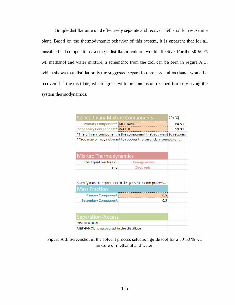
125

Simple distillation would effectively separate and recover methanol for re-use in a

plant. Based on the thermodynamic behavior of this system, it is apparent that for all

possible feed compositions, a single distillation column would effective. For the 50-50 %

wt. methanol and water mixture, a screenshot from the tool can be seen in Figure A 3,

which shows that distillation is the suggested separation process and methanol would be

recovered in the distillate, which agrees with the conclusion reached from observing the

system thermodynamics.

Figure A 3. Screenshot of the solvent process selection guide tool for a 50-50 % wt.

mixture of methanol and water.

126

Not all mixtures that require only simple distillation as the separation process

have the same thermodynamic behavior. In the 1,2-dimethoxyethane/water system in

Figure A 5, the n-hexane/n-methyl-2-pyrrolidone systems in Figure A 6 and Figure A 7,

the desired solvent can effectively be purified with distillation, even though these

mixtures have different thermodynamic behavior.

Figure A 4. Illustration of a purification process for a 50-50% mixture of water and

methanol to obtain methanol by distillation.

20

30

40

50

60

70

80

90

100

110

0 0.1 0.2 0.3 0.4 0.5 0.6 0.7 0.8 0.9 1

Tem

pe

ratu

re (

°C)

Methanol Mass Fraction

Liquid

Vapor

127

Figure A 5. Illustration of a purification process for a 95 % wt. mixture of 1,2-

dimethoxyethane in water to obtain 1,2-dimethoxyethane by distillation.

Figure A 6. Illustration of a purification process for a 10 % wt. mixture of n-hexane in n-

methyl-2-pyrrolidone to obtain n-hexane by distillation.

20

30

40

50

60

70

80

90

100

110

0 0.1 0.2 0.3 0.4 0.5 0.6 0.7 0.8 0.9 1

Tem

pe

ratu

re (

°C)

1,2 dimethoxyethane Mass Fraction

Vapor

Liquid

20

40

60

80

100

120

140

160

180

200

0 0.1 0.2 0.3 0.4 0.5 0.6 0.7 0.8 0.9 1

Tem

pe

ratu

re (

°C)

N-hexane Mass Fraction

Vapor

Liquid

Liquid-Liquid

128

Figure A 7. Illustration of a purification process for a 90 % wt. mixture of n-hexane in n-

methyl-2-pyrrolidone to obtain n-hexane by distillation.

The second separation process that can be suggested by the tool is distillation

followed by either a pervaporation or azeotropic distillation. Such is the case of a 25 %

wt. mixture of 1,2-dimethoxyethane in water as seen in the vapor-liquid equilibrium

diagram of Figure A 8.

20

40

60

80

100

120

140

160

180

200

0 0.1 0.2 0.3 0.4 0.5 0.6 0.7 0.8 0.9 1

Tem

pe

ratu

re (

°C)

N-hexane Mass Fraction

Vapor

Liquid

Liquid-Liquid

129

Figure A 8. Illustration of a purification process for a 25 % wt. mixture of 1,2-

dimethoxyethane in water to obtain 1,2-dimethoxyethane by distillation to the azeotrope

and then either pervaporation or azeotropic distillation to the purity desired.

A representative block flow diagram for the purification process of the 25 % wt.

mixture of 1,2-dimethoxyethane can be seen in Figure A 9. The case assumes a 25 % wt.

mixture of 1,2-dimethoxyethane is fed to a distillation column, which produces a water

bottoms product and an approximately 90 % wt. azeotropic mixture of 1,2-

dimethoxyethane. This azeotropic mixture can then be fed either to a pervaporation

system or an azeotropic distillation process to dehydrate the mixture and obtain 1,2-

dimethoxyethane product to be recycled back to the pharmaceutical process.

20

30

40

50

60

70

80

90

100

110

0 0.1 0.2 0.3 0.4 0.5 0.6 0.7 0.8 0.9 1

Tem

pe

ratu

re (

°C)

1,2 dimethoxyethane Mass Fraction

Vapor

Liquid

130

Figure A 9. Process flow diagram for a 25 % wt. mixture of 1,2-dimethoxyethane in

water. Mass fractions shown are mass fractions of 1,2-dimethoxyethane in the mixture.

Concentrations shown are for illustrative purposes.

When using the solvent recovery selection guide tool, the user will input the two

solvents, 1,2-dimethoxyethane and water, and a mass fraction of 0.25 for 1,2-

dimethoxyethane. This results in the screenshot seen in Figure A 10. The suggested

separation process from the solvent recovery selection guide matches the process

determined by studying the system thermodynamics (Figure A 8).

FeedX = 0.25

Water

Water

1,2-dimethoxyethane

AzeotropeX = 0.55

Vacuum Pump

Pervaporation Unit

Azeotropic Distillation Option

Distillation Column

131

Figure A 10. Screenshot of the recovery process selection guide for a 25 % wt. mixture of

1,2-dimethoxyethane in water. Cells that require user input are highlighter in orange.

A binary mixture of 2-methyltetrahydrofuran (2-MeTHF) and water, is

heterogeneous between 10 to 94 % wt. of 2-MeTHF at 25 °C (Figure A 11). If the feed

mixture is within this heterogeneous range, the first step in the separation process would

use a decanter to separate the two liquid phases.

132

Figure A 11. A vapor-liquid equilibrium diagram for the water and n-butanol binary

mixture at 1 atm created using Aspen Plus® Binary Analysis.

For a 50-50% mixture of 2-MeTHF and water, it can be seen from Figure A 12

that the mixture is heterogeneous which is indicated by the fact that the liquid equilibrium

line is horizontal from approximately 10-94 % wt. 2-MeTHF. From this, the ideal first

step in the separation process would use a decanter to separate the two liquid phases.

Exiting the decanter will be an aqueous stream containing approximately 10 % wt. 2-

MeTHF and an organic stream containing approximately 94 % wt. 2-MeTHF. The

organic stream would then need to be further purified with distillation in order to be

recycled. A representative block diagram for this process can be seen in Figure A 13.

20

30

40

50

60

70

80

90

100

110

0 0.1 0.2 0.3 0.4 0.5 0.6 0.7 0.8 0.9 1

Tem

per

atu

re (

°C)

2-MeTHF Mass Fraction

Vapor

Liquid

Liquid-Liquid

133

Figure A 12. Illustration of a purification process for a 50-50 % wt. mixture of water and

2-MeTHF to obtain 2-MeTHF by decanting and then distillation.

Figure A 13. Separation Process for a 50-50 % wt. mixture of 2-MeTHF and water. Mass

fractions (X) shown are the mass fractions of 2-MeTHF in the mixture. Concentrations

shown are for illustrative purposes.

20

30

40

50

60

70

80

90

100

110

0 0.1 0.2 0.3 0.4 0.5 0.6 0.7 0.8 0.9 1

Tem

per

atu

re (

°C)

2-MeTHF Mass Fraction

Vapor

Liquid

Liquid-Liquid

FeedX = 0.5

MeTHF

AzeotropeX = 0.9

Aqueous phase(heavy phase)X = 0.1

organic phase(light phase)X = 0.94

DecanterDistillationColumn

134

Figure A 14. User interface for the recovery process selection guide. Shown is a 50-50 %

wt. feed mixture of 2-MeTHF and water. Cells that require user input are highlighted in

orange.

As seen in Figure A 14 the suggested separation process for this case is a decanter

followed by distillation.

The fourth separation process that the recovery process selection guide provides is

a decanter, followed by a distillation column, followed by either a pervaporation unit or

an azeotropic distillation unit. One example mixture that would require this recovery

process is a 50-50 % wt. mixture of 1-propanol and water. From the vapor-liquid

equilibrium diagram in Figure A 15 it is clear that the thermodynamics for this mixture

are more complex than previous mixtures mentioned due to the location of the azeotrope

outside of the heterogeneous range. Figure A 16 shows the recovery process for this

BP (°C)

2-MeTHF 80.3

WATER 99.99

*The primary component is the component that you want to recover.

**You may or may not want to recover the secondary component.

The liquid mixture is Heterogeneous between X1 = 0.104 and X2 = 0.9416 at 25 °C and 1 atm, where "X" is the mass fraction of the primary component.

and Azeotropic at X = 0.908 and T = 71.65 °C at P = 1 atm, where "X" is the mass fraction of the primary component.

Specify mass composition to design separation process…

Mass Fraction0.5

0.5

DECANTER + DISTILLATION or PERVAPORATION

The light phase of the decanter is sent to distillation where 2-MeTHF is recovered in the bottoms

Select Binary Mixture Components

Mixture Thermodynamics

Separation Process

Primary Component*

Secondary Component**

Primary Component

Secondary Component

135

mixture. A decanter would first be used to split the two liquid phases that are formed,

producing an organic phase with approximately 65 % wt. 1-propanol. After the decanter,

a distillation column could be used to get to the azeotrope (~70 % wt. 1-propanol), and

lastly a pervaporation unit or an azeotropic distillation system could be used to get past

the azeotrope and reach the desired purity. A block flow diagram for this process can be

seen in Figure A 17. The suggested recovery process by the recovery selection process

guide agrees with this thermodynamic analysis, as seen in Figure A 18.

Figure A 15. Vapor-liquid equilibrium diagram for a binary mixture of 1-propanol and

water created using Aspen Plus®

.

20

30

40

50

60

70

80

90

100

110

0 0.1 0.2 0.3 0.4 0.5 0.6 0.7 0.8 0.9 1

Tem

pe

ratu

re (

°C)

1-propanol Mass Fraction

Vapor

Liquid

Liquid-Liquid

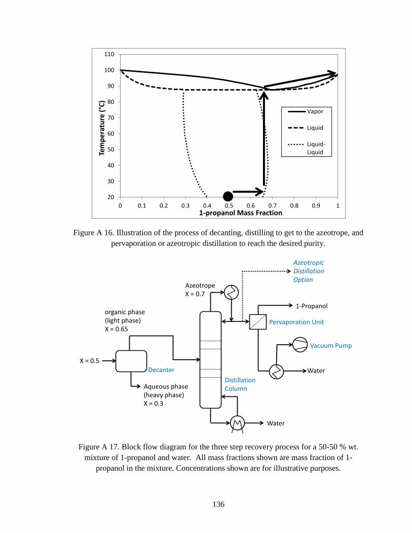
136

Figure A 16. Illustration of the process of decanting, distilling to get to the azeotrope, and

pervaporation or azeotropic distillation to reach the desired purity.

Figure A 17. Block flow diagram for the three step recovery process for a 50-50 % wt.

mixture of 1-propanol and water. All mass fractions shown are mass fraction of 1-

propanol in the mixture. Concentrations shown are for illustrative purposes.

20

30

40

50

60

70

80

90

100

110

0 0.1 0.2 0.3 0.4 0.5 0.6 0.7 0.8 0.9 1

Tem

pe

ratu

re (

°C)

1-propanol Mass Fraction

Vapor

Liquid

Liquid-Liquid

X = 0.5

Water

Azeotrope X = 0.7

Aqueous phase(heavy phase)X = 0.3

organic phase(light phase)X = 0.65

Decanter Water

1-Propanol

Vacuum Pump

Pervaporation Unit

Azeotropic Distillation Option

DistillationColumn

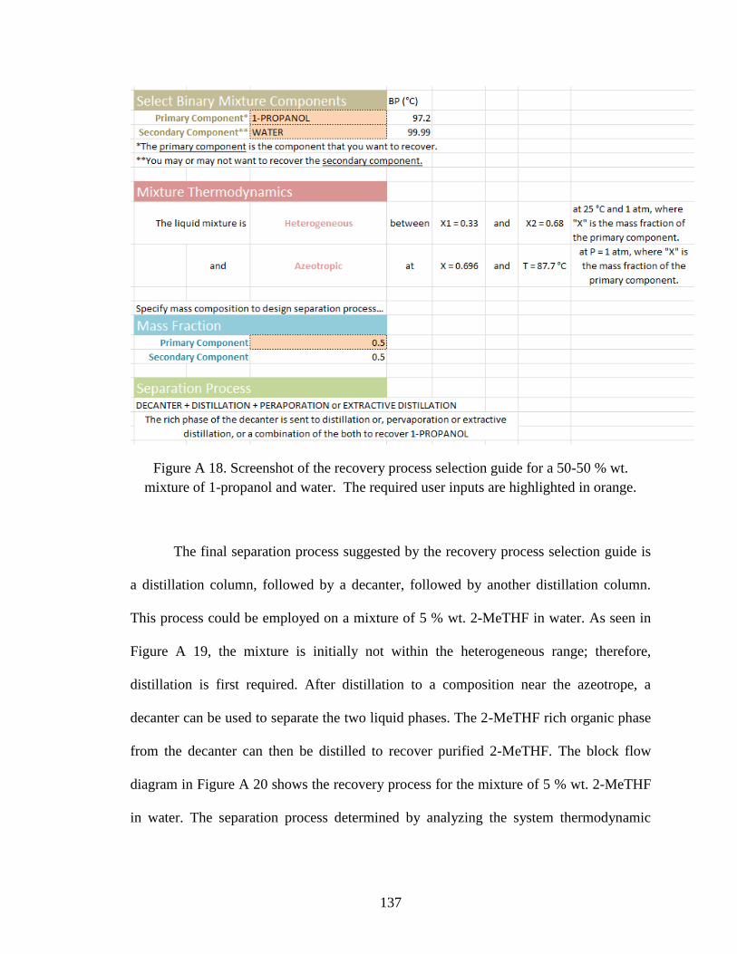
137

Figure A 18. Screenshot of the recovery process selection guide for a 50-50 % wt.

mixture of 1-propanol and water. The required user inputs are highlighted in orange.

The final separation process suggested by the recovery process selection guide is

a distillation column, followed by a decanter, followed by another distillation column.

This process could be employed on a mixture of 5 % wt. 2-MeTHF in water. As seen in

Figure A 19, the mixture is initially not within the heterogeneous range; therefore,

distillation is first required. After distillation to a composition near the azeotrope, a

decanter can be used to separate the two liquid phases. The 2-MeTHF rich organic phase

from the decanter can then be distilled to recover purified 2-MeTHF. The block flow

diagram in Figure A 20 shows the recovery process for the mixture of 5 % wt. 2-MeTHF

in water. The separation process determined by analyzing the system thermodynamic

138

behavior matches the suggested separation by the Recovery Process Selection Guide in

Figure A 21.

Figure A 19. Illustration of a purification process for a 5 % wt. mixture of 2-MeTHF in

water. (1) Distillation from 5 % wt. 2-MeTHF to ~90 % wt. (2) Decanter to separate two

liquid phases of the heterogeneous mixture. (3) Distillation to achieve purified 2-MeTHF.

Figure A 20. Separation process for a 5 wt. % mixture of 2-MeTHF in water. Mass

fractions shown are the mass fractions of 2-MeTHF in the mixture. Concentrations shown

are for illustrative purposes.

20

30

40

50

60

70

80

90

100

110

0 0.1 0.2 0.3 0.4 0.5 0.6 0.7 0.8 0.9 1

Tem

per

atu

re (

°C)

2-MeTHF Mass Fraction

Vapor

Liquid

Liquid-Liquid

FeedX = 0.05

MeTHF

AzeotropeX = 0.9

aqueous phase(heavy phase)X = 0.1

organic phase(light phase)X = 0.94

Decanter

Water

AzeotropeX = 0.9

DistillationColumn

DistillationColumn

139

Figure A 21. User interface for the recovery process selection guide. Shown is a 5 % wt.

feed mixture of 2-MeTHF in water. Cells that require user input are highlighted in

orange.

BP (°C)

2-MeTHF 80.3

WATER 99.99

*The primary component is the component that you want to recover.

**You may or may not want to recover the secondary component.

The liquid mixture is Heterogeneous between X1 = 0.104 and X2 = 0.9416 at 25 °C and 1 atm, where "X" is the mass fraction of the primary component.

and Azeotropic at X = 0.908 and T = 71.65 °C at P = 1 atm, where "X" is the mass fraction of the primary component.

Specify mass composition to design separation process…

Mass Fraction0.05

0.95

DISTILLATION 1 + DECANTER + DISTILLATION 2

The first distillation produces a distillate heterogeneous stream that is decanted. The light phase is further distilled and

2-MeTHF is recovered in the bottoms

Select Binary Mixture Components

Mixture Thermodynamics

Separation Process

Primary Component*

Secondary Component**

Primary Component

Secondary Component

140

Appendix C

UNIQUAC Thermodynamic Behavior Prediction vs. Experimental Data

In the following figures, the vapor liquid equilibrium prediction using UNIQUAC as the

thermodynamic property method is compared with experimental data. The letter “x”

refers to the mole fraction in the liquid, and “y” refers to the mole fraction in the gas. The

experimental data references are shown at the bottom of the figures.

Acetone-Acetonitrile

Figure A 22. P-x-y vapor-liquid equilibrium diagram for acetone and acetonitrile at a

constant temperature of 45 °C. Experimental data reference: Brown I., Smith F.: Austr. J.

Chem. 13, 30 (1960).

200

250

300

350

400

450

500

550

0 0,1 0,2 0,3 0,4 0,5 0,6 0,7 0,8 0,9 1

P (

mm

Hg)

x ,y (mole fraction, acetone)

(T = 45 °C)

x (experimental)

y (experimental)

x (UNIQUAC)

y (UNIQUAC)

141

Figure A 23. x-y vapor-liquid equilibrium diagram for acetone and acetonitrile at a

constant temperature of 45 °C. Experimental data reference: Brown I., Smith F.: Austr. J.

Chem. 13, 30 (1960).

IPA-THF

Figure A 24. T-x-y vapor-liquid equilibrium diagram for IPA and THF at a constant

pressure of 1 atm. Experimental data reference: Sheblom T.V.: Liquid-Vapor Equilibrium

in the System Tetrahydrofuran-Isopropyl Alcohol. Zh.Prikl.Khim. 42 (1969) 2389-2390.

0

0,1

0,2

0,3

0,4

0,5

0,6

0,7

0,8

0,9

1

0 0,1 0,2 0,3 0,4 0,5 0,6 0,7 0,8 0,9 1

y (v

apo

r m

ole

fra

ctio

n, a

ceto

ne

)

x (liquid mole fraction, acetone)

T = 45 °C

Experimental

UNIQUAC

65

67

69

71

73

75

77

79

81

83

85

0 0,1 0,2 0,3 0,4 0,5 0,6 0,7 0,8 0,9 1

T (°

C)

x,y (mole fraction, THF)

P = 1 atm

x (experimental)

y (experimental)

x (UNIQUAC)

y (UNIQUAC)

142

Figure A 25. x-y vapor-liquid equilibrium diagram for IPA and THF at a constant

pressure of 1 atm. Experimental data reference: Sheblom T.V.: Liquid-Vapor Equilibrium

in the System Tetrahydrofuran-Isopropyl Alcohol. Zh.Prikl.Khim. 42 (1969) 2389-2390.

Acetone-Toluene

Figure A 26. P-x-y vapor-liquid equilibrium diagram for acetone and toluene at a constant

temperature of 30 °C. Experimental data reference: Hopkins,J.A., V.R.Bhethanabotla and

S.W.Campbell, J.Chem.Eng.Data, 39, 488 (1994).

0

0,1

0,2

0,3

0,4

0,5

0,6

0,7

0,8

0,9

1

0 0,1 0,2 0,3 0,4 0,5 0,6 0,7 0,8 0,9 1

y (m

ole

fra

ctio

n in

vap

or,

TH

F)

x (mole fraction in liquid, THF)

P = 1 atm

Experimental

UNIQUAC

0

5

10

15

20

25

30

35

40

0 0,1 0,2 0,3 0,4 0,5 0,6 0,7 0,8 0,9 1

P (

kPa)

x,y (mole fraction, acetone)

T = 30 °C

x (experimental)

y (experimental)

x (UNIQUAC)

y (UNIQUAC)

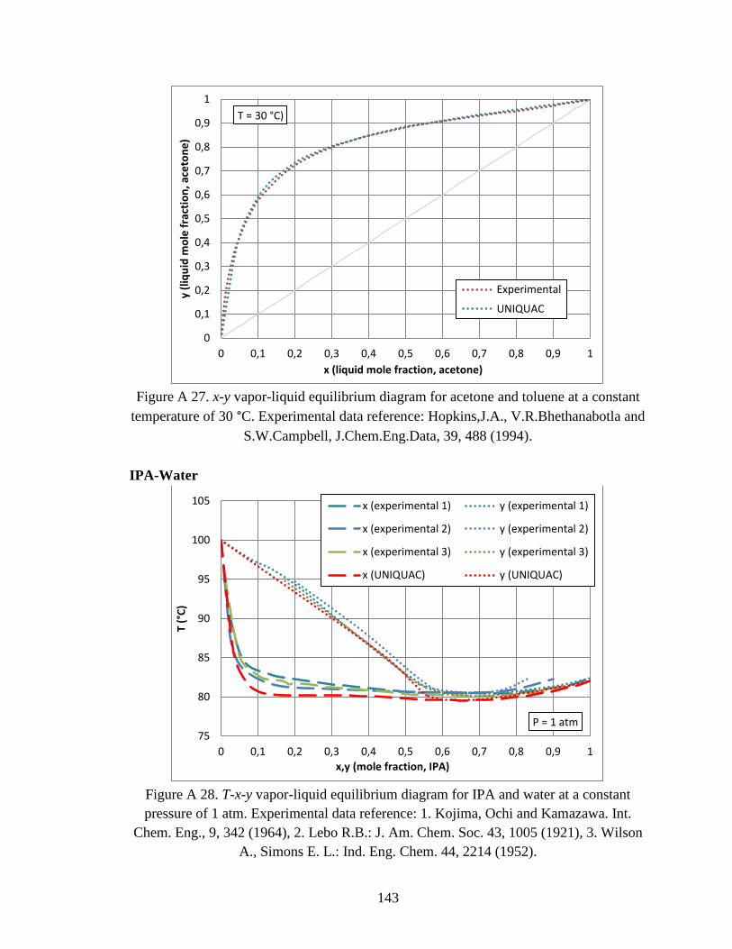
143

Figure A 27. x-y vapor-liquid equilibrium diagram for acetone and toluene at a constant

temperature of 30 °C. Experimental data reference: Hopkins,J.A., V.R.Bhethanabotla and

S.W.Campbell, J.Chem.Eng.Data, 39, 488 (1994).

IPA-Water

Figure A 28. T-x-y vapor-liquid equilibrium diagram for IPA and water at a constant

pressure of 1 atm. Experimental data reference: 1. Kojima, Ochi and Kamazawa. Int.

Chem. Eng., 9, 342 (1964), 2. Lebo R.B.: J. Am. Chem. Soc. 43, 1005 (1921), 3. Wilson

A., Simons E. L.: Ind. Eng. Chem. 44, 2214 (1952).

0

0,1

0,2

0,3

0,4

0,5

0,6

0,7

0,8

0,9

1

0 0,1 0,2 0,3 0,4 0,5 0,6 0,7 0,8 0,9 1

y (l

iqu

id m

ole

fra

ctio

n, a

ceto

ne

)

x (liquid mole fraction, acetone)

T = 30 °C)

Experimental

UNIQUAC

75

80

85

90

95

100

105

0 0,1 0,2 0,3 0,4 0,5 0,6 0,7 0,8 0,9 1

T (°

C)

x,y (mole fraction, IPA)

P = 1 atm

x (experimental 1) y (experimental 1)

x (experimental 2) y (experimental 2)

x (experimental 3) y (experimental 3)

x (UNIQUAC) y (UNIQUAC)

144

Figure A 29. x-y vapor-liquid equilibrium diagram for IPA and water at a constant

pressure of 1 atm. Experimental data reference: 1. Kojima, Ochi and Kamazawa. Int.

Chem. Eng., 9, 342 (1964), 2. Lebo R.B.: J. Am. Chem. Soc. 43, 1005 (1921), 3. Wilson

A., Simons E. L.: Ind. Eng. Chem. 44, 2214 (1952).

0

0,1

0,2

0,3

0,4

0,5

0,6

0,7

0,8

0,9

1

0 0,1 0,2 0,3 0,4 0,5 0,6 0,7 0,8 0,9 1

y (v

apo

r m

ole

fra

ctio

n, I

PA

)

x (liquid mole fraction, IPA)

P = 1 atm

Experimental 1

Experimental 2

Experimental 3

UNIQUAC

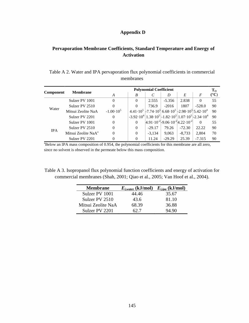
145

Appendix D

Pervaporation Membrane Coefficients, Standard Temperature and Energy of

Activation

Table A 2. Water and IPA pervaporation flux polynomial coefficients in commercial

membranes

Component Membrane Polynomial Coefficient TO

(°C) A B C D E F

Water

Sulzer PV 1001 0 0 2.555 -5.356 2.838 0 55

Sulzer PV 2510 0 0 736.9 -2016 1807 -528.0 90

Mitsui Zeolite NaA -1.00·105 4.41·10

5 -7.74·10

5 6.68·10

5 -2.98·10

5 5.42·10

4 90

Sulzer PV 2201 0 -3.92·104

1.38·105 -1.82·10

5 1.07·10

5 -2.34·10

4 90

IPA

Sulzer PV 1001 0 0 4.91·10-2

-9.06·10-2

4.22·10-2

0 55

Sulzer PV 2510 0 0 -29.17 79.26 -72.30 22.22 90

Mitsui Zeolite NaAa

0 0 -3,134 9,063 -8,733 2,804 70

Sulzer PV 2201 0 0 11.24 -29.29

25.39

-7.315

90 aBelow an IPA mass composition of 0.954, the polynomial coefficients for this membrane are all zero,

since no solvent is observed in the permeate below this mass composition.

Table A 3. Isopropanol flux polynomial function coefficients and energy of activation for

commercial membranes (Shah, 2001; Qiao et al., 2005; Van Hoof et al., 2004).

Membrane Ei,water (kJ/mol) Ei,ipa (kJ/mol)

Sulzer PV 1001 44.46 35.67

Sulzer PV 2510 43.6 81.10

Mitsui Zeolite NaA 68.39 36.88

Sulzer PV 2201 62.7 94.90

146

Appendix E

Diagram representation of pervaporation calculations

Figure A 30. Diagram representation of pervaporation membrane area, mass balance and

energy balance calculation procedure

T1 xs,1A F

Components Properties

Js,1, Jw,1

P1

R1xs,2 AComponents Properties

J1

ys,1

T2

Area

Block 1

Area

Block 2

.

.

.

Area

Block N

(1)

(7)

(7)(14)

(15) (4)

RN-1xs,N AComponents Properties

TN

(16)

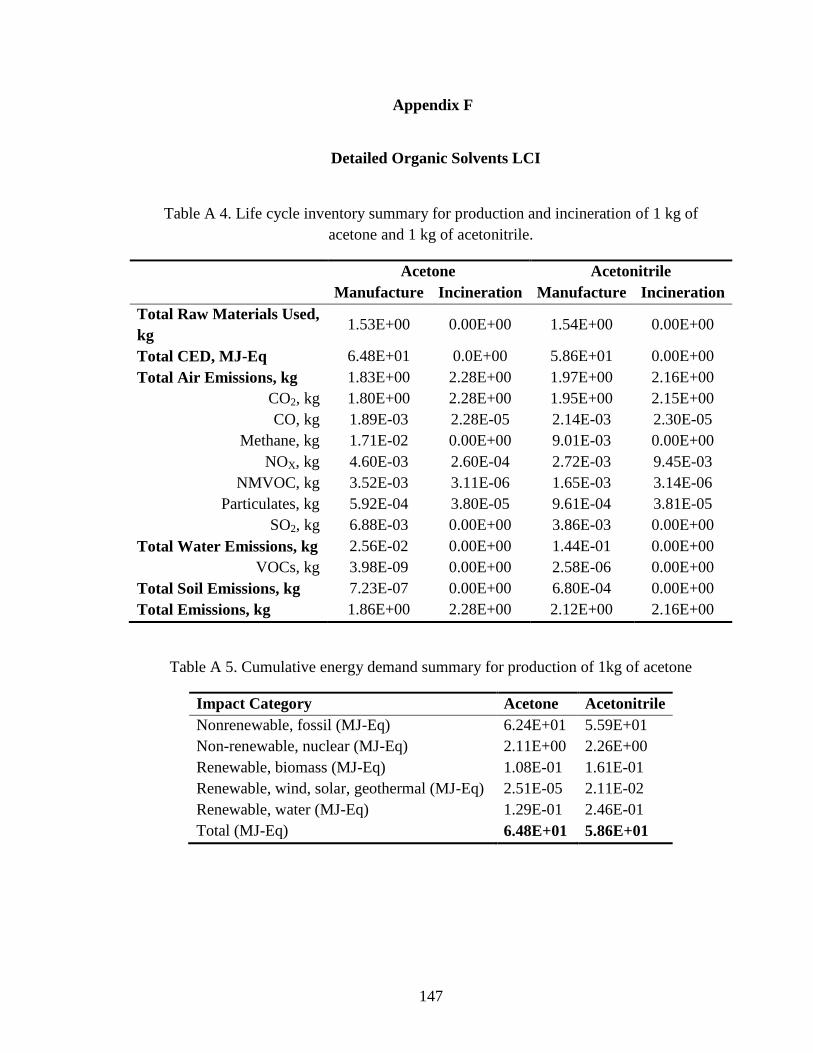
147

Appendix F

Detailed Organic Solvents LCI

Table A 4. Life cycle inventory summary for production and incineration of 1 kg of

acetone and 1 kg of acetonitrile.

Acetone Acetonitrile

Manufacture Incineration Manufacture Incineration

Total Raw Materials Used,

kg 1.53E+00 0.00E+00 1.54E+00 0.00E+00

Total CED, MJ-Eq 6.48E+01 0.0E+00 5.86E+01 0.00E+00

Total Air Emissions, kg 1.83E+00 2.28E+00 1.97E+00 2.16E+00

CO2, kg 1.80E+00 2.28E+00 1.95E+00 2.15E+00

CO, kg 1.89E-03 2.28E-05 2.14E-03 2.30E-05

Methane, kg 1.71E-02 0.00E+00 9.01E-03 0.00E+00

NOX, kg 4.60E-03 2.60E-04 2.72E-03 9.45E-03

NMVOC, kg 3.52E-03 3.11E-06 1.65E-03 3.14E-06

Particulates, kg 5.92E-04 3.80E-05 9.61E-04 3.81E-05

SO2, kg 6.88E-03 0.00E+00 3.86E-03 0.00E+00

Total Water Emissions, kg 2.56E-02 0.00E+00 1.44E-01 0.00E+00

VOCs, kg 3.98E-09 0.00E+00 2.58E-06 0.00E+00

Total Soil Emissions, kg 7.23E-07 0.00E+00 6.80E-04 0.00E+00

Total Emissions, kg 1.86E+00 2.28E+00 2.12E+00 2.16E+00

Table A 5. Cumulative energy demand summary for production of 1kg of acetone

Impact Category Acetone Acetonitrile

Nonrenewable, fossil (MJ-Eq) 6.24E+01 5.59E+01

Non-renewable, nuclear (MJ-Eq) 2.11E+00 2.26E+00

Renewable, biomass (MJ-Eq) 1.08E-01 1.61E-01

Renewable, wind, solar, geothermal (MJ-Eq) 2.51E-05 2.11E-02

Renewable, water (MJ-Eq) 1.29E-01 2.46E-01

Total (MJ-Eq) 6.48E+01 5.86E+01

148

Table A 6. Life cycle inventory for the manufacture and incineration of 1 kg IPA and 1kg

of THF.

IPA THF

Manufacture Incineration Manufacture Incineration

Total Raw Materials Used, kg 1.55E+00 0.00E+00 4.01E+00 0.00E+00

Total CED, MJ-Eq 6.01E+01 0.00E+00 1.28E+02 0.00E+00

Total Air Emissions, kg 1.66E+00 2.21E+00 5.52E+00 2.45E+00

CO2, kg 1.63E+00 2.20E+00 5.46E+00 2.44E+00

CO, kg 2.25E-03 2.26E-05 4.82E-03 2.33E-05

Methane, kg 9.72E-03 0.00E+00 1.45E-02 0.00E+00

NOX, kg 2.67E-03 2.59E-04 8.67E-03 2.62E-04

NMVOC, kg 1.75E-03 3.09E-06 3.25E-03 3.18E-06

Particulates, kg 8.40E-04 3.78E-05 3.57E-03 3.84E-05

SO2, kg 5.36E-03 0.00E+00 1.15E-02 0.00E+00

Total Water Emissions, kg 5.42E-01 0.00E+00 1.26E-01 0.00E+00

VOCs, kg 1.08E-06 0.00E+00 7.93E-06 0.00E+00

Total Soil Emissions, kg 3.18E-04 0.00E+00 2.31E-03 0.00E+00

Total Emissions, kg 2.20E+00 2.21E+00 5.65E+00 2.45E+00

Table A 7. Cumulative energy demand summary for the manufacture of 1kg of IPA and 1

kg of THF

Impact category IPA THF

Nonrenewable, fossil (MJ-Eq) 5.73E+01 1.11E+02

Non-renewable, nuclear (MJ-Eq) 2.38E+00 1.31E+01

Renewable, biomass (MJ-Eq) 1.75E-01 6.02E-01

Renewable, wind, solar, geothermal (MJ-Eq) 2.24E-02 2.10E-01

Renewable, water (MJ-Eq) 2.31E-01 2.04E+00

Total (MJ-Eq) 6.01E+01 1.28E+02

149

Table A 8. Life cycle inventory summary for the manufacture and incineration of 1 kg

toluene

Manufacture Incineration

Total Raw Materials Used, kg 1.36E+00 0.00E+00

Total CED, MJ-Eq 6.19E+01 0.00E+00

Total Air Emissions, kg 1.21E+00 3.36E+00

CO2, kg 1.19E+00 3.35E+00

CO, kg 2.05E-03 2.28E-05

Methane, kg 1.23E-02 0.00E+00

NOX, kg 2.06E-03 2.59E-04

NMVOC, kg 1.88E-03 3.11E-06

Particulates, kg 3.97E-04 3.79E-05

SO2, kg 2.28E-03 0.00E+00

Total Water Emissions, kg 3.87E-03 0.00E+00

VOCs, kg 1.95E-09 0.00E+00

Total Soil Emissions, kg 3.46E-07 0.00E+00

Total Emissions, kg 1.21E+00 3.36E+00

Table A 9. Cumulative energy demand summary for the manufacture of 1kg of toluene

Impact category Total

Nonrenewable, fossil (MJ-Eq) 6.05E+01

Non-renewable, nuclear (MJ-Eq) 1.29E+00

Renewable, biomass (MJ-Eq) 8.50E-02

Renewable, wind, solar, geothermal (MJ-Eq) 1.16E-05

Renewable, water (MJ-Eq) 5.34E-02

Total (MJ-Eq) 6.19E+01

150

Table A 10. ecoTHFTM

and ecoMeTHFTM

Incineration LCI

Total Raw Materials Used, kg 1.39E-03

Total CED, MJ-Eq -6.50E-01

Total Air Emissions, kg 8.15E-03

CO2, kg 0.00E+00

CO, kg 2.32E-05

Methane, kg 0.00E+00

NOX, kg 2.61E-04

NMVOC, kg 3.16E-06

Particulates, kg 3.83E-05

SO2, kg 0.00E+00

Total Water Emissions, kg 0.00E+00

VOCs, kg 0.00E+00

Total Soil Emissions, kg 0.00E+00

Total Emissions, kg 8.15E-03

151

Appendix G

Utilities LCI

Kalamazoo Plant Utilities: Selamectin, Nelfinavir and Hydrocortisone Cases.

The method used in SimaPro®

to calculate the electricity LCI was Eco-indicator

99 “H” (hierarchical). The power generating station that supplies electricity for the

Kalamazoo plant uses a mixed fuel. SimaPro®

has a method which was selected to

calculate emissions based on mixed fuels. The electricity from fuel was calculated based

on current US technologies. No technology description is provided because the dataset

only describes the power plant generation portfolio of the country using current average

technology per energy carrier. The process for the production of electricity does not

include transformation or transportation as specified by the program. The total emissions,

total raw materials used, and the energy used for the production of electricity can be seen

in Table A 11.

152

Table A 11. Life cycle inventory for 1 kWh of electricity at Kalamazoo plant (US

production mix)

Total Raw Materials Used, kg 3.98E-01

Total CED, MJ-Eq 3.60E+00

Total Air Emissions, kg 7.36E-01

CO2, kg 7.27E-01

CO, kg 2.89E-04

Methane, kg 1.35E-03

NOX, kg 1.43E-03

NMVOC, kg 1.06E-04

Particulates, kg 6.65E-04

SO2, kg 3.94E-03

Total Water Emissions, kg 2.63E-02

VOCs, kg 3.59E-07

Total Soil Emissions, kg 9.05E-05

Total Emissions, kg 7.62E-01

The simulation was run on a basis of 1 kWh of electricity generated. The majority

of emissions, a total of 96%, are to the air with emissions to water and soil making up the

final 4%. Of the 0.736 kg of air emissions, 0.727 kg of air emissions are attributed to CO2

with a variety of greenhouse gases and other components making up the remaining 0.009

kg. The total energy used for the process is 3.6 MJ-Eq and a summary of the sources of

this energy can be seen in Table A 12. This electricity LCI was used for all Pfizer case

studies presented.

A life cycle inventory was also completed for the production of 1 kg of steam

from coal. The steam for the Kalamazoo plant is obtained from coal and is produced on-

site. To produce 1 kg of steam at 170 psig, 0.0952 kg of coal is used. This is the basis that

is used for the LCI. This LCI was also completed using SimaPro®

by method of Eco-

indicator 99 “H”. Coal is used in industrial boilers to make steam. The technologies used

for the simulation are not specified but it is stated that current average US technology

153

data are used. The data are for the cradle-to-gate resource requirements and emissions for

the combustion of coal. As stated earlier, the simulation was run on a 0.0952 kg basis for

coal and this can be seen in Table A 13.

Table A 12. Cumulative energy demand for 1 kWh electricity

Impact Category Total

Nonrenewable, fossil (MJ-Eq) 2.50E+00

Non-renewable, nuclear (MJ-Eq) 9.10E-01

Renewable, biomass (MJ-Eq) 3.67E-02

Renewable, wind, solar, geothermal (MJ-Eq) 4.11E-03

Renewable, water (MJ-Eq) 7.65E-02

Total (MJ-Eq) 3.60E+00

Table A 13. Life cycle inventory for production of 1 kg of steam at 170 psig from coal

Total Raw Materials Used, kg 1.02E-01

Total CED, MJ-Eq 2.57E+00

Total Air Emissions, kg 2.32E-01

CO2, kg 2.29E-01

CO, kg 8.95E-05

Methane, kg 4.54E-04

NOX, kg 5.36E-04

NMVOC, kg 1.44E-05

Particulates, kg 3.02E-04

Total Water Emissions, kg 1.88E-04

Total Soil Emissions, kg 9.63E-05

Total Emissions, kg 2.32E-01

The total raw materials needed to make 0.0952 kg of coal is 0.102 kg. The total

emissions to the air come to 0.232 kg. This is to combust only 0.0952 kg of coal. This

process produces approximately two and a half times more emissions than the amount of

coal used. CO2 makes up 0.229 kg of the total air emissions. The large proportion of air

emissions causes the emissions to water and soil to become negligible in terms of the

154

total emissions. The total energy used to combust the coal is 2.57 MJ-Eq and a summary

of the energy can be seen in Table A 14. This analysis includes the combustion of coal to

make steam, which is included in the LCI. In addition, Table A 14 shows that no energy

for the process is produced from a renewable source. All of the energy supplied is from

non-renewable fossil fuels and nuclear energy.

Table A 14. Cumulative energy demand for the combustion of 0.0952 kg of coal

Impact Category Total

Non-renewable, fossil (MJ-Eq) 2.56E+00

Non-renewable, nuclear (MJ-Eq) 5.23E-03

Renewable, biomass (MJ-Eq) 0.00E+00

Renewable, wind, solar, geothermal (MJ-Eq) 0.00E+00

Renewable, water (MJ-Eq) 0.00E+00

Total (MJ-Eq) 2.57E+00

Barceloneta Plant Utilities: Celecoxib Case

Table A 15. Life Cycle Inventory for 1 kg of Saturated Steam at 125 psig and 1 kWh of

electricity at the Barceloneta Plant

Saturated Steam at 125 psig 1 kWh of electricity

Total Raw Materials, kg 8.00E-02 3.47E-01

Total CED, MJ-Eq 3.40E+00 3.56E+00

Total Air Emissions, kg 2.57E-01 8.86E-01

CO2, kg 2.49E-01 8.76E-01

CO, kg 1.37E-03 2.67E-03

Methane, kg 3.03E-04 1.54E-03

NOX, kg 4.48E-03 1.66E-03

NMVOC, kg 1.55E-03 4.08E-04

Particulates, kg 1.03E-04 3.01E-04

SO2, kg 3.75E-04 1.96E-03

Total Water Emissions, kg 3.99E-03 9.64E-02

VOCs - 3.20E-08

Total Soil Emissions, kg 1.73E-04 1.20E-05

Total Emissions, kg 2.61E-01 9.83E-01

155

Average Chemical Plant Utilities: ecoTHFTM

and ecoMeTHFTM

recoveries

Table A 16. Life Cycle Inventory for 1 kg of Saturated Steam at 125 psig and 1 kWh of

electricity at the Barceloneta Plant

Total Raw Materials Used, kg 9.02E-02

Total CED, MJ-Eq 3.92E+00

Total Air Emissions, kg 2.24E-01

CO2 2.23E-01

CO 5.84E-05

Methane 4.51E-04

NOx 2.00E-04

NMVOC 6.04E-05

Particulates 4.61E-05

SO2 3.82E-04

Total Water Emissions, kg 2.31E-03

VOCs 3.91E-07

Total Soil Emissions, kg 9.63E-05

Total Emissions, kg 2.26E-01

156

Appendix H

LCA Results of Case Studies

Table A 17. Base process selamectin process LCA

Manufacture

Acetonitrile

Manufacture

Acetone

Incineration

Acetonitrile

Incineration

Acetone Total

Amount Used, kg 60,840 23,660 60,840 23,660 -

Total Raw Materials Used,

kg 9.35E+04 3.61E+04 * * 1.30E+05

Total CED, MJ-Eq 3.57E+06 1.53E+06 0.00E+00 0.00E+00 5.10E+06

Total Air Emissions, kg 1.20E+05 4.33E+04 1.32E+05 5.40E+04 3.49E+05

CO2, kg 1.18E+05 4.25E+04 1.31E+05 5.39E+04 3.45E+05

CO, kg 1.30E+02 4.47E+01 1.40E+00 5.40E-01 1.77E+02

Methane, kg 5.48E+02 4.05E+02 0.00E+00 0.00E+00 9.53E+02

NOX, kg 1.66E+02 1.09E+02 5.75E+02 6.15E+00 8.56E+02

NMVOC, kg 1.00E+02 8.34E+01 1.91E-01 7.36E-02 1.84E+02

Particulates, kg 5.84E+01 1.40E+01 2.32E+00 8.98E-01 7.57E+01

SO2, kg 2.35E+02 1.63E+02 0.00E+00 0.00E+00 3.98E+02

Total Water Emissions, kg 8.79E+03 6.05E+02 0.00E+00 0.00E+00 9.39E+03

VOCs, kg 1.57E-01 9.41E-05 0.00E+00 0.00E+00 1.57E-01

Total Soil Emissions, kg 4.14E+01 1.71E-02 0.00E+00 0.00E+00 4.14E+01

Total Emissions, kg 1.29E+05 4.39E+04 1.32E+05 5.40E+04 3.59E+05

*Air is used in incineration; however the amount cannot be quantified

157

Table A 18. Acetonitrile recovery process LCA

Manufacture Incineration Saturated

Steam @

170 psig

Electricity Total Acetonitrile Acetone Acetonitrile Acetone

Amount Used, kg

or *kWh 9,671 23,660 9,671 23,660 105,350 *16,301 -

Total Raw

Materials Used, kg 1.48E+04 3.60E+04 0.00E+00 0.00E+00 1.07E+04 6.49E+03 6.80E+04

Total CED, MJ-Eq 5.66E+05 1.53E+06 0.00E+00 0.00E+00 2.71E+05 5.87E+04 2.44E+06

Total Air

Emissions, kg 1.89E+04 4.32E+04 2.08E+04 5.40E+04 2.44E+04 1.20E+04 1.73E+05

CO2, kg 1.87E+04 4.24E+04 2.06E+04 5.39E+04 2.41E+04 1.19E+04 1.71E+05

CO, kg 2.06E+01 4.46E+01 2.21E-01 5.40E-01 9.43E+00 4.71E+00 8.01E+01

Methane, kg 8.66E+01 4.04E+02 0.00E+00 0.00E+00 4.78E+01 2.20E+01 5.60E+02

NOX, kg 2.62E+01 1.09E+02 9.09E+01 6.15E+00 5.65E+01 2.33E+01 3.12E+02

NMVOC, kg 1.59E+01 8.32E+01 3.02E-02 7.36E-02 1.52E+00 1.73E+00 1.02E+02

Particulates, kg 9.24E+00 1.40E+01 3.67E-01 8.98E-01 3.18E+01 1.08E+01 6.71E+01

SO2, kg 3.71E+01 1.62E+02 0.00E+00 0.00E+00 0.00E+00 6.42E+01 2.63E+02

Total Water

Emissions, kg 1.39E+03 6.03E+02 0.00E+00 0.00E+00 1.98E+01 4.29E+02 2.44E+03

VOCs, kg 2.48E-02 9.38E-05 0.00E+00 0.00E+00 0.00E+00 5.85E-03 3.07E-02

Total Soil

Emissions, kg 6.54E+00 1.71E-02 0.00E+00 0.00E+00 9.53E+00 1.48E+00 1.76E+01

Total Emissions, kg 2.03E+04 4.38E+04 2.08E+04 5.40E+04 2.45E+04 1.24E+04 1.76E+05

158

Table A 19. Base process vs. acetonitrile recovery LCA

Base Process Recovery Process Reduction* % Reduction

Total Raw Materials Used, kg 1.30E+05 6.80E+04 6.20E+04 47.69%

Total CED, MJ-Eq 5.10E+06 2.44E+06 2.66E+06 52.15%

Total Air Emissions, kg 3.49E+05 1.73E+05 1.76E+05 50.43%

CO2, kg 3.45E+05 1.71E+05 1.74E+05 50.43%

CO, kg 1.77E+02 8.01E+01 9.69E+01 54.75%

Methane, kg 9.53E+02 5.60E+02 3.93E+02 41.24%

NOX, kg 8.56E+02 3.12E+02 5.44E+02 63.55%

NMVOC, kg 1.84E+02 1.02E+02 8.20E+01 44.57%

Particulates, kg 7.57E+01 6.71E+01 8.60E+00 11.36%

SO2, kg 3.98E+02 2.63E+02 1.35E+02 33.92%

Total Water Emissions, kg 9.39E+03 2.44E+03 6.95E+03 74.01%

VOCs, kg 1.57E-01 3.07E-02 1.26E-01 80.45%

Total Soil Emissions, kg 4.14E+01 1.76E+01 2.38E+01 57.49%

Total Emissions, kg 3.59E+05 1.76E+05 1.83E+05 50.97%

*The reduction column contains the avoided emissions.

Table A 20. Acetone recovery LCA

Manufacture

Acetone

Incineration

Acetone

Sat'd Steam

@ 170 psig Electricity Total

Amount Used, kg or

*kWh 3,101 3,101 33,249 *5,181 -

Total Raw Materials

Used, kg 4.73E+03 0.00E+00 3.39E+03 2.06E+03 1.02E+04

Total CED, MJ-Eq 2.01E+05 0.00E+00 8.54E+04 1.87E+04 3.05E+05

Total Air Emissions, kg 5.67E+03 7.08E+03 7.71E+03 3.81E+03 2.43E+04

CO2, kg 5.57E+03 7.06E+03 7.61E+03 3.77E+03 2.40E+04

CO, kg 5.86E+00 7.07E-02 2.98E+00 1.50E+00 1.04E+01

Methane, kg 5.30E+01 0.00E+00 1.51E+01 6.99E+00 7.51E+01

NOX, kg 1.43E+01 8.06E-01 1.78E+01 7.41E+00 4.03E+01

NMVOC, kg 1.09E+01 9.64E-03 4.79E-01 5.49E-01 1.20E+01

Particulates, kg 1.84E+00 1.18E-01 1.00E+01 3.45E+00 1.54E+01

SO2, kg 2.13E+01 0.00E+00 0.00E+00 2.04E+01 4.17E+01

Total Water Emissions,

kg 7.92E+01 0.00E+00 6.25E+00 1.36E+02 2.22E+02

VOCs, kg 1.23E-05 0.00E+00 0.00E+00 1.86E-03 1.87E-03

Total Soil Emissions, kg 2.24E-03 0.00E+00 3.01E+00 4.69E-01 3.48E+00

Total Emissions, kg 5.75E+03 7.08E+03 7.72E+03 3.95E+03 2.45E+04

159

Table A 21. Acetonitrile and acetone recovery process LCA

Manufacture Incineration Saturated

Steam @

170 psig

Electricity Total Acetonitrile Acetone Acetonitrile Acetone

Amount Used, kg

or *kWh 9,671 3,101 9,671 3,101 138,599 *21,482 -

Total Raw

Materials Used, kg 1.48E+04 4.73E+03 0.00E+00 0.00E+00 1.41E+04 8.55E+03 4.22E+04

Total CED, MJ-Eq 5.66E+05 2.01E+05 0.00E+00 0.00E+00 3.56E+05 7.74E+04 1.20E+06

Total Air

Emissions, kg 1.89E+04 5.67E+03 2.08E+04 7.08E+03 3.21E+04 1.58E+04 1.00E+05

CO2, kg 1.87E+04 5.57E+03 2.06E+04 7.06E+03 3.17E+04 1.57E+04 9.93E+04

CO, kg 2.06E+01 5.86E+00 2.21E-01 7.07E-02 1.24E+01 6.21E+00 4.54E+01

Methane, kg 8.66E+01 5.30E+01 0.00E+00 0.00E+00 6.29E+01 2.90E+01 2.31E+02

NOX, kg 2.62E+01 1.43E+01 9.09E+01 8.06E-01 7.43E+01 3.07E+01 2.37E+02

NMVOC, kg 1.59E+01 1.09E+01 3.02E-02 9.64E-03 2.00E+00 2.28E+00 3.11E+01

Particulates, kg 9.24E+00 1.84E+00 3.67E-01 1.18E-01 4.18E+01 1.43E+01 6.76E+01

SO2, kg 3.71E+01 2.13E+01 0.00E+00 0.00E+00 0.00E+00 8.46E+01 1.43E+02

Total Water

Emissions, kg 1.39E+03 7.92E+01 0.00E+00 0.00E+00 2.61E+01 5.65E+02 2.06E+03

VOCs, kg 2.48E-02 1.23E-05 0.00E+00 0.00E+00 0.00E+00 7.71E-03 3.25E-02

Total Soil

Emissions, kg 6.54E+00 2.24E-03 0.00E+00 0.00E+00 1.25E+01 1.95E+00 2.10E+01

Total Emissions, kg 2.03E+04 5.75E+03 2.08E+04 7.08E+03 3.22E+04 1.64E+04 1.03E+05

Table A 22. Base process and recovery process LCA comparison

Base Process Recovery Process Reduction % Reduction

Total Raw Materials Used, kg 1.30E+05 4.22E+04 8.78E+04 67.54%

Total CED, MJ-Eq 5.10E+06 1.20E+06 3.90E+06 76.47%

Total Air Emissions, kg 3.49E+05 1.00E+05 2.49E+05 71.35%

CO2, kg 3.45E+05 9.93E+04 2.46E+05 71.22%

CO, kg 1.77E+02 4.54E+01 1.32E+02 74.35%

Methane, kg 9.53E+02 2.31E+02 7.22E+02 75.76%

NOX, kg 8.56E+02 2.37E+02 6.19E+02 72.31%

NMVOC, kg 1.84E+02 3.11E+01 1.53E+02 83.10%

Particulates, kg 7.57E+01 6.76E+01 8.10E+00 10.70%

SO2, kg 3.98E+02 1.43E+02 2.55E+02 64.07%

Total Water Emissions, kg 9.39E+03 2.06E+03 7.33E+03 78.06%

VOCs, kg 1.57E-01 3.25E-02 1.24E-01 79.30%

Total Soil Emissions, kg 4.14E+01 2.10E+01 2.04E+01 49.28%

Total Emissions, kg 3.59E+05 1.03E+05 2.56E+05 71.31%

160

Table A 23. Nelfinavir case, base process LCA

Manufacture

IPA

Incineration

IPA

Manufacture

THF

Incineration

THF Total

Amount Used, kg 67,682 67,682 11,018 11,018 -

Total Raw Materials Used,

kg 1.05E+05 * 4.42E+04 * 1.49E+05

Total CED, MJ-Eq 4.07E+06 0.00E+00 1.41E+06 0.00E+00 5.48E+06

Total Air Emissions, kg 1.12E+05 1.49E+05 6.08E+04 2.70E+04 3.49E+05

CO2, kg 1.10E+05 1.49E+05 6.02E+04 2.69E+04 3.46E+05

CO, kg 1.53E+02 1.53E+00 5.32E+01 2.57E-01 2.07E+02

Methane, kg 6.58E+02 0.00E+00 1.60E+02 0.00E+00 8.18E+02

NOX, kg 1.81E+02 1.75E+01 9.56E+01 2.88E+00 2.97E+02

NMVOC, kg 1.18E+02 2.09E-01 3.58E+01 3.50E-02 1.54E+02

Particulates, kg 5.69E+01 2.56E+00 3.93E+01 4.23E-01 9.92E+01

SO2, kg 3.63E+02 0.00E+00 1.27E+02 0.00E+00 4.90E+02

Total Water Emissions, kg 3.67E+04 0.00E+00 1.39E+03 0.00E+00 3.81E+04

VOCs, kg 7.29E-02 0.00E+00 8.74E-02 0.00E+00 1.60E-01

Total Soil Emissions, kg 2.16E+01 0.00E+00 2.54E+01 0.00E+00 4.70E+01

Total Emissions, kg 1.49E+05 1.49E+05 6.22E+04 2.70E+04 3.88E+05

* Air is used in incineration; however the amount cannot be quantified

Table A 24. Nelfinavir case, IPA recovery process LCA

Manufacture Incineration Sat'd Steam

@ 170 psig Electricity Total

IPA THF IPA THF

Amount, kg or *kWh 5,148 11,018 5,148 11,018 73,505 *10,953 -

Total Raw Materials Used,

kg 7.97E+03 4.42E+04 0.00E+00 0.00E+00 7.50E+03 4.36E+03 6.40E+04

Total CED, MJ-Eq 3.10E+05 1.41E+06 0.00E+00 0.00E+00 1.89E+05 3.94E+04 1.95E+06

Total Air Emissions, kg 8.53E+03 6.08E+04 1.14E+04 2.70E+04 1.71E+04 8.06E+03 1.33E+05

CO2, kg 8.39E+03 6.02E+04 1.13E+04 2.69E+04 1.68E+04 7.96E+03 1.32E+05

CO, kg 1.16E+01 5.32E+01 1.17E-01 2.57E-01 6.58E+00 3.17E+00 7.49E+01

Methane, kg 5.01E+01 1.60E+02 0.00E+00 0.00E+00 3.34E+01 1.48E+01 2.58E+02

NOX, kg 1.38E+01 9.56E+01 1.33E+00 2.88E+00 3.94E+01 1.57E+01 1.69E+02

NMVOC, kg 9.00E+00 3.58E+01 1.59E-02 3.50E-02 1.06E+00 1.16E+00 4.70E+01

Particulates, kg 4.32E+00 3.93E+01 1.94E-01 4.23E-01 2.22E+01 7.28E+00 7.38E+01

SO2, kg 2.76E+01 1.27E+02 0.00E+00 0.00E+00 0.00E+00 4.32E+01 1.98E+02

Total Water Emissions, kg 2.79E+03 1.39E+03 0.00E+00 0.00E+00 1.38E+01 2.88E+02 4.48E+03

VOCs, kg 5.54E-03 8.74E-02 0.00E+00 0.00E+00 0.00E+00 3.93E-03 9.68E-02

Total Soil Emissions, kg 1.64E+00 2.54E+01 0.00E+00 0.00E+00 7.08E+00 9.91E-01 3.51E+01

Total Emissions, kg 1.13E+04 6.22E+04 1.14E+04 2.70E+04 1.71E+04 8.35E+03 1.37E+05

161

Table A 25. Hydrocortisone case base process LCA

Manufacture

Toluene

Manufacture

Acetone

Incineration

Toluene

Incineration

Acetone Total

Amount Used, kg 233,913 23,687 233,913 23,687

Total Raw Materials Used,

kg 3.17E+05 3.62E+04 * * 3.54E+05

Total CED, MJ-Eq 1.45E+07 1.54E+06 0.00E+00 0.00E+00 1.60E+07

Total Air Emissions, kg 2.83E+05 4.34E+04 7.85E+05 5.41E+04 1.17E+06

CO2, kg 2.78E+05 4.25E+04 7.83E+05 5.39E+04 1.16E+06

CO, kg 4.79E+02 4.47E+01 5.33E+00 5.40E-01 5.30E+02

Methane, kg 2.88E+03 4.05E+02 0.00E+00 0.00E+00 3.28E+03

NOX, kg 4.83E+02 1.09E+02 6.07E+01 6.15E+00 6.58E+02

NMVOC, kg 4.39E+02 8.35E+01 7.27E-01 7.37E-02 5.23E+02

Particulates, kg 9.30E+01 1.40E+01 8.86E+00 8.99E-01 1.17E+02

SO2, kg 5.33E+02 1.63E+02 0.00E+00 0.00E+00 6.96E+02

Total Water Emissions, kg 9.04E+02 6.05E+02 0.00E+00 0.00E+00 1.51E+03

VOCs, kg 4.56E-04 9.42E-05 0.00E+00 0.00E+00 5.50E-04

Total Soil Emissions, kg 8.09E-02 1.71E-02 0.00E+00 0.00E+00 9.81E-02

Total Emissions, kg 2.84E+05 4.40E+04 7.85E+05 5.41E+04 1.17E+06

* Air is used in incineration; however the amount cannot be quantified

Table A 26. Total LCA for toluene and acetone recovery in Hydrocortisone case

Sat'd Steam @

170 psig Electricity Total

Amount Used, kg or *kWh

Total Raw Materials Used, kg 5.78E+03 2.47E+03 8.25E+03

Total CED, MJ-Eq 1.46E+05 2.23E+04 1.68E+05

Total Air Emissions, kg 1.32E+04 4.57E+03 1.77E+04

CO2, kg 1.30E+04 4.51E+03 1.75E+04

CO, kg 5.07E+00 1.79E+00 6.87E+00

Methane, kg 2.57E+01 8.38E+00 3.41E+01

NOX, kg 3.04E+01 8.87E+00 3.93E+01

NMVOC, kg 8.16E-01 6.58E-01 1.47E+00

Particulates, kg 1.71E+01 4.13E+00 2.12E+01

SO2, kg 0.00E+00 2.44E+01 2.44E+01

Total Water Emissions, kg 1.07E+01 1.63E+02 1.74E+02

VOCs, kg 0.00E+00 2.23E-03 2.23E-03

Total Soil Emissions, kg 5.46E+00 5.62E-01 6.02E+00

Total Emissions, kg 1.32E+04 4.73E+03 1.79E+04

162

Table A 27. Hydrocortisone case base process toluene and acetone recovery LCA

Base

Process

Recovery

Process Reduction % Reduction

Total Raw Materials Used, kg 3.54E+05 8.25E+03 3.45E+05 97.67%

Total CED, MJ-Eq 1.60E+07 1.68E+05 1.58E+07 98.95%

Total Air Emissions, kg 1.17E+06 1.77E+04 1.15E+06 98.48%

CO2, kg 1.16E+06 1.75E+04 1.14E+06 98.49%

CO, kg 5.30E+02 6.87E+00 5.23E+02 98.70%

Methane, kg 3.28E+03 3.41E+01 3.25E+03 98.96%

NOX, kg 6.58E+02 3.93E+01 6.19E+02 94.04%

NMVOC, kg 5.23E+02 1.47E+00 5.22E+02 99.72%

Particulates, kg 1.17E+02 2.12E+01 9.55E+01 81.80%

SO2, kg 6.96E+02 2.44E+01 6.71E+02 96.49%

Total Water Emissions, kg 1.51E+03 1.74E+02 1.34E+03 88.48%

VOCs, kg 5.50E-04 2.23E-03 -1.68E-03 -304.76%

Total Soil Emissions, kg 9.81E-02 6.02E+00 -5.92E+00 -6034.66%

Total Emissions, kg 1.17E+06 1.79E+04 1.15E+06 98.47%

Table A 28. Base process LCA for IPA-Water

Manufacture

IPA

Manufacture

Water

Incineration

IPA

Incineration

Water Total

Amount Used, kg 2,560,845 2,905,539 2,560,845 2,905,539

Total Raw Materials Used, kg 3.97E+06 2.58E+03 * * 3.97E+06

Total CED, MJ-Eq 1.54E+08 3.50E+04 0.00E+00 0.00E+00 1.54E+08

Total Air Emissions, kg 4.24E+06 1.99E+03 5.66E+06 9.88E+06 1.98E+07

CO2, kg 4.18E+06 1.97E+03 5.63E+06 9.86E+06 1.97E+07

CO, kg 5.77E+03 3.83E+00 5.80E+01 6.59E+01 5.90E+03

Methane, kg 2.49E+04 3.36E+00 0.00E+00 0.00E+00 2.49E+04

NOX, kg 6.84E+03 3.13E+00 6.63E+02 7.53E+02 8.26E+03

NMVOC, kg 4.48E+03 3.04E-01 7.91E+00 8.98E+00 4.49E+03

Particulates, kg 2.15E+03 1.93E+00 9.67E+01 1.10E+02 2.36E+03

SO2, kg 1.37E+04 5.15E+00 0.00E+00 0.00E+00 1.37E+04

Total Water Emissions, kg 1.39E+06 1.40E+03 0.00E+00 0.00E+00 1.39E+06

VOCs, kg 2.76E+00 1.52E-03 0.00E+00 0.00E+00 2.76E+00

Total Soil Emissions, kg 8.15E+02 3.48E-01 0.00E+00 0.00E+00 8.16E+02

Total Emissions, kg 5.63E+06 3.39E+03 5.66E+06 9.88E+06 2.12E+07

* Air is used in incineration; however the amount cannot be quantified

163

Table A 29. LCA for IPA recovery process

Manufacture Incineration Sat'd Steam

@ 125 psig Electricity Total

IPA Water IPA Water

Amount Used, kg or

*kWh 12,438 2,905,539 12,438 2,905,539 5,112,607 *811,348

Total Raw Materials

Used, kg 1.93E+04 2.58E+03 * * 4.09E+05 2.82E+05 7.12E+05

Total CED, MJ-Eq 7.48E+05 3.50E+04 0.00E+00 0.00E+00 1.74E+07 2.89E+06 2.11E+07

Total Air Emissions, kg 2.06E+04 1.99E+03 2.75E+04 9.88E+06 1.31E+06 7.19E+05 1.20E+07

CO2, kg 2.03E+04 1.97E+03 2.74E+04 9.86E+06 1.27E+06 7.11E+05 1.19E+07

CO, kg 2.80E+01 3.83E+00 2.82E-01 6.59E+01 7.00E+03 2.17E+03 9.27E+03

Methane, kg 1.21E+02 3.36E+00 0.00E+00 0.00E+00 1.55E+03 1.25E+03 2.92E+03

NOX, kg 3.32E+01 3.13E+00 3.22E+00 7.53E+02 2.29E+04 1.35E+03 2.50E+04

NMVOC, kg 2.17E+01 3.04E-01 3.84E-02 8.98E+00 7.92E+03 3.31E+02 8.29E+03

Particulates, kg 1.04E+01 1.93E+00 4.70E-01 1.10E+02 5.27E+02 2.44E+02 8.93E+02

SO2, kg 6.67E+01 5.15E+00 0.00E+00 0.00E+00 1.92E+03 1.59E+03 3.58E+03

Total Water Emissions,

kg 6.74E+03 1.40E+03 0.00E+00 0.00E+00 2.04E+04 7.82E+04 1.07E+05

VOCs, kg 1.34E-02 1.52E-03 0.00E+00 0.00E+00 0.00E+00 2.60E-02 4.09E-02

Total Soil Emissions, kg 3.96E+00 3.48E-01 0.00E+00 0.00E+00 8.84E+02 9.74E+00 8.99E+02

Total Emissions, kg 2.74E+04 3.39E+03 2.75E+04 9.88E+06 1.33E+06 7.98E+05 1.21E+07

Table A 30. IPA-water base process and recovery process comparison

Base

Process

Recovery

Process Reduction % Reduction

Total Raw Materials Used, kg 3.97E+06 7.12E+05 3.26E+06 82.06%

Total CED, MJ-Eq 1.54E+08 2.11E+07 1.33E+08 86.36%

Total Air Emissions, kg 1.98E+07 1.20E+07 7.84E+06 39.59%

CO2, kg 1.97E+07 1.19E+07 7.81E+06 39.65%

CO, kg 5.90E+03 9.27E+03 -3.37E+03 -57.09%

Methane, kg 2.49E+04 2.92E+03 2.20E+04 88.26%

NOX, kg 8.26E+03 2.50E+04 -1.68E+04 -203.19%

NMVOC, kg 4.49E+03 8.29E+03 -3.80E+03 -84.56%

Particulates, kg 2.36E+03 8.93E+02 1.47E+03 62.14%

SO2, kg 1.37E+04 3.58E+03 1.01E+04 73.87%

Total Water Emissions, kg 1.39E+06 1.07E+05 1.28E+06 92.32%

VOCs, kg 2.76E+00 4.09E-02 2.72E+00 98.52%

Total Soil Emissions, kg 8.16E+02 8.99E+02 -8.25E+01 -10.11%

Total Emissions, kg 2.12E+07 1.21E+07 9.13E+06 43.07%

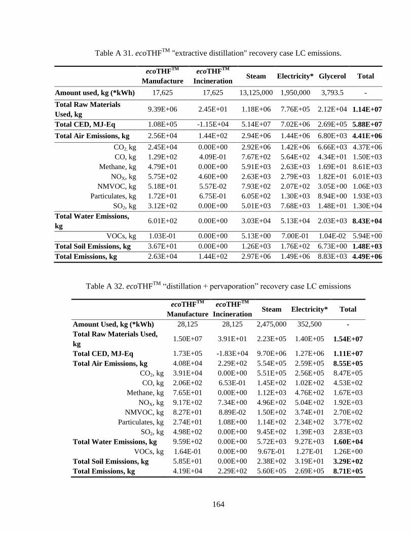
164

Table A 31. ecoTHFTM

"extractive distillation" recovery case LC emissions.

ecoTHF

TM

Manufacture

ecoTHFTM

Incineration Steam Electricity* Glycerol Total

Amount used, kg (*kWh) 17,625 17,625 13,125,000 1,950,000 3,793.5 -

Total Raw Materials

Used, kg 9.39E+06 2.45E+01 1.18E+06 7.76E+05 2.12E+04 1.14E+07

Total CED, MJ-Eq 1.08E+05 -1.15E+04 5.14E+07 7.02E+06 2.69E+05 5.88E+07

Total Air Emissions, kg 2.56E+04 1.44E+02 2.94E+06 1.44E+06 6.80E+03 4.41E+06

CO2, kg 2.45E+04 0.00E+00 2.92E+06 1.42E+06 6.66E+03 4.37E+06

CO, kg 1.29E+02 4.09E-01 7.67E+02 5.64E+02 4.34E+01 1.50E+03

Methane, kg 4.79E+01 0.00E+00 5.91E+03 2.63E+03 1.69E+01 8.61E+03

NOX, kg 5.75E+02 4.60E+00 2.63E+03 2.79E+03 1.82E+01 6.01E+03

NMVOC, kg 5.18E+01 5.57E-02 7.93E+02 2.07E+02 3.05E+00 1.06E+03

Particulates, kg 1.72E+01 6.75E-01 6.05E+02 1.30E+03 8.94E+00 1.93E+03

SO2, kg 3.12E+02 0.00E+00 5.01E+03 7.68E+03 1.48E+01 1.30E+04

Total Water Emissions,

kg 6.01E+02 0.00E+00 3.03E+04 5.13E+04 2.03E+03 8.43E+04

VOCs, kg 1.03E-01 0.00E+00 5.13E+00 7.00E-01 1.04E-02 5.94E+00

Total Soil Emissions, kg 3.67E+01 0.00E+00 1.26E+03 1.76E+02 6.73E+00 1.48E+03

Total Emissions, kg 2.63E+04 1.44E+02 2.97E+06 1.49E+06 8.83E+03 4.49E+06

Table A 32. ecoTHFTM

“distillation + pervaporation” recovery case LC emissions

ecoTHFTM

Manufacture

ecoTHFTM

Incineration Steam Electricity* Total

Amount Used, kg (*kWh) 28,125 28,125 2,475,000 352,500 -

Total Raw Materials Used,

kg 1.50E+07 3.91E+01 2.23E+05 1.40E+05 1.54E+07

Total CED, MJ-Eq 1.73E+05 -1.83E+04 9.70E+06 1.27E+06 1.11E+07

Total Air Emissions, kg 4.08E+04 2.29E+02 5.54E+05 2.59E+05 8.55E+05

CO2, kg 3.91E+04 0.00E+00 5.51E+05 2.56E+05 8.47E+05

CO, kg 2.06E+02 6.53E-01 1.45E+02 1.02E+02 4.53E+02

Methane, kg 7.65E+01 0.00E+00 1.12E+03 4.76E+02 1.67E+03

NOX, kg 9.17E+02 7.34E+00 4.96E+02 5.04E+02 1.92E+03

NMVOC, kg 8.27E+01 8.89E-02 1.50E+02 3.74E+01 2.70E+02

Particulates, kg 2.74E+01 1.08E+00 1.14E+02 2.34E+02 3.77E+02

SO2, kg 4.98E+02 0.00E+00 9.45E+02 1.39E+03 2.83E+03

Total Water Emissions, kg 9.59E+02 0.00E+00 5.72E+03 9.27E+03 1.60E+04

VOCs, kg 1.64E-01 0.00E+00 9.67E-01 1.27E-01 1.26E+00

Total Soil Emissions, kg 5.85E+01 0.00E+00 2.38E+02 3.19E+01 3.29E+02

Total Emissions, kg 4.19E+04 2.29E+02 5.60E+05 2.69E+05 8.71E+05

165

Table A 33. ecoMeTHFTM

recovery LC emissions

ecoMeTHFTM

Manufacture

ecoMeTHFTM

Incineration Steam Electricity* Total

Amount used, kg (*kWh) 37,500 37,500 1,837,500 217,500 -

Total Raw Materials Used,

kg 4.54E+06 5.21E+01 1.66E+05 8.66E+04 4.79E+06

Total CED, MJ-Eq -7.50E+05 -2.44E+04 7.20E+06 7.83E+05 7.21E+06

Total Air Emissions, kg 6.08E+03 3.06E+02 4.12E+05 1.60E+05 5.78E+05

CO2, kg 5.63E+03 0.00E+00 4.09E+05 1.58E+05 5.73E+05

CO, kg 2.49E+02 8.70E-01 1.07E+02 6.29E+01 4.20E+02

Methane, kg -3.52E+01 0.00E+00 8.28E+02 2.94E+02 1.09E+03

NOX, kg 5.18E+02 9.79E+00 3.68E+02 3.11E+02 1.21E+03

NMVOC, kg 9.23E+01 1.19E-01 1.11E+02 2.31E+01 2.26E+02

Particulates, kg 4.73E+01 1.44E+00 8.46E+01 1.45E+02 2.78E+02

SO2, kg -1.71E+02 0.00E+00 7.02E+02 8.57E+02 1.39E+03

Total Water Emissions, kg 1.02E+03 0.00E+00 4.25E+03 5.72E+03 1.10E+04

VOCs, kg 2.09E-01 0.00E+00 7.18E-01 7.81E-02 1.00E+00

Total Soil Emissions, kg 7.28E+01 0.00E+00 1.77E+02 1.97E+01 2.69E+02

Total Emissions, kg 7.16E+03 3.06E+02 4.16E+05 1.66E+05 5.89E+05

Table A 34. ecoMeTHFTM

recovery LC emissions comparison.

Chemical THF

Base Case

ecoMeTHFTM

Recovery Case

Emissions

Reduction

Total Raw Materials Used, kg 1.50E+07 4.79E+06 1.02E+07

Total CED, MJ-Eq 4.93E+08 7.21E+06 4.86E+08

Total Air Emissions, kg 2.99E+07 5.78E+05 2.93E+07

CO2, kg 2.96E+07 5.73E+05 2.90E+07

CO, kg 1.82E+04 4.20E+02 1.78E+04

Methane, kg 5.44E+04 1.09E+03 5.33E+04

NOX, kg 3.35E+04 1.21E+03 3.23E+04

NMVOC, kg 1.22E+04 2.26E+02 1.20E+04

Particulates, kg 1.35E+04 2.78E+02 1.32E+04

SO2, kg 4.31E+04 1.39E+03 4.17E+04

Total Water Emissions, kg 4.73E+05 1.10E+04 4.62E+05

VOCs, kg 2.97E+01 1.00E+00 2.87E+01

Total Soil Emissions, kg 8.66E+03 2.69E+02 8.39E+03

Total Emissions, kg 3.04E+07 5.89E+05 2.98E+07

166

Appendix I

Detailed Economic Results of Case Studies

Table A 35. Economic analysis of acetonitrile recovery in the selamectin process based

on annual operating costs

Base Process Recovery Process Savings

Acetone Purchased ($/year) 24,370 24,370 0

Acetonitrile Purchased ($/year) 247,619 39,361 208,258

Incineration ($/year) 10,901 4,300 6,601

Distillation Utilities ($/year) -- 3,737 -3,737

Total ($/year) 282,890 71,768 211,122

Table A 36. Economic analysis of acetone recovery in the selamectin process based on

annual operating costs

Base Process Recovery Process Savings

Acetone Purchased ($/year) 24,370 3,194 21,176

Incineration ($/year) 3,052 400 2,652

Distillation Utilities ($/year) -- 1,183 -1,183

Total ($/year) 27,422 4,777 22,645

Table A 37. Economic analysis of acetonitrile and acetone recovery in the selamectin

process based on annual operating costs

Base Process Recovery Process Savings

Acetone Purchased ($/year) 24,370 3,194 21,176

Acetonitrile Purchased ($/year) 247,619 39,361 208,258

Incineration ($/year) 10,901 1,648 9,253

Distillation Utilities ($/year) -- 4,920 -4,920

Total ($/year) 282,890 49,123 233,767

167

Table A 38. Economic analysis of toluene recovery in Hydrocortisone case based on

annual operating costs

Base Process Recovery Process Savings

Acetone Purchased ($/year) 24,398 - 24,398

Toluene Purchased ($/year) 215,200 - 215,200

Incineration ($/year) 33,230 - 33,230

Distillation Utilities ($/year) -- 1,754 -1,754

Total ($/year) 272,828 1,754 271,074

Table A 39. Economic analysis of IPA recovered based on annual operating costs

Base Process Recovery Process Savings

Isopropanol Purchased ($/year) 2,361,099 11,468 2,349,631

Incineration ($/year) 2,733,192 1,458,989 1,274,203

Distillation Utilities ($/year) -- 307,545 -307,545

Total ($/year) 5,094,291 1,778,002 3,316,289

168

Appendix J

Skid Investment Cost Calculation

Three distillation column vendor quotations, including the corresponding column

dimensions and characteristics, are presented in Table A 40. Given the column

dimensions and characteristics, it was assumed that the quotations could be used to

estimate a packed column of 20 ft. in height and 1.5 ft. in diameter, including auxiliary

equipment. These quotations were provided in February 2010. Assuming an inflation of

2.5 %a, the average cost of these quotations in 2013 would be:

* ( )

+ (

)

( )

If we assume that the shipment and installation cost is 100% of the capital cost, then the

final cost would be US$ 1,507,647.

Table A 40. Distillation column vendor quotations

Company Quote

a

(US$)

Estimation

Range

Diam.

(ft.)

Height

(ft.)

Reboiler

(ft2)

Condenser

(ft2)

Preheater

(ft2)

Other

ARTISANb 400,000 +/-30% 1 25 50 50 20 packed

APVc

875,000 - 2 19 NSd

NSd

NAe

trays

KMPSf

825,000 +/-20% 1 27 25 35 NAc

packed

aAll quotations are F.O.B. and include bottoms and distillate/reflux pumps, and other auxiliary equipment

such as instruments, valves, piping, relief valves, etc. bIncludes a feed pump, a 20 ft

2 preheater and a distillate accumulator.

cSize: 10x12x35 ft., in WxLxH. Includes a reflux pump, besides the distillate.

d Not Specified

e Not Available

f Includes a 35 gallon reflux drum and a 10 ft

2 preheater. The approximate height is 35 ft.

In January 2003, the cost of Sulzer type pervaporation units containing PERVAP®

2510 type membranes, with a membrane area of 70 m2 and 140 m

2 was 390,000 and

480,000 euros, respectively. The equipment size cost exponent is therefore:

(

)

( )

a http://www.tradingeconomics.com/united-states/inflation-cpi, June 2013.

169

In January 2003, the cost of the euro was 1.05 dollarsb. Therefore, a 140 m

2

pervaporation unit costed, in 2003, US$ 504,000. Accounting for an inflation of 2.5 %,

the cost in 2013 would be:

(

)

( )

A pervaporation unit with 210 m2 of membrane area would have a cost of:

(

)

Assuming a shipment and installation cost of 100 % the capital cost, the final

pervaporation unit cost would be US$ 1,456,965.

Therefore, a skid containing a distillation and pervaporation unit as described

above would cost:

b http://www.oanda.com/currency/historical-rates/

170

Appendix K

Underwood Minimum Reflux Ratio Calculation

The following Underwood minimum-reflux equations were used:

∑

and

∑

were:

is the relative volatility of component i to the reference component, and is

calculated as:

o , were N is the number of stages, and

o

, were r is the reference component.

is the distillate molar fraction of component i,

is calculated using the second Underwood equation,

is the minimum reflux ratio,

is the molar fraction in the feed of component i,

and q is defined as:

171

o

, were is the feed enthalpy at the

saturated vapor state, is the feed enthalpy at the saturated liquid

state, and is the real feed enthalpy.

Table A 41 shows the calculation of the Rm for the selamectin and hydrocortisone

cases, with the equations shown above. The distillate molar fractions and the feed

enthalpies were obtained from Aspen Plus®

. For the hydrocortisone case, xD is defined as

the specification acetone purity, but in the hydrocortisone case, xD is the result of

obtaining the required acetonitrile purity in the bottoms. The value of was guessed to

satisfy the second Underwood equation until the difference between both sides of the

equation was smaller than a magnitude of 10-7

. The difference is shown as the Dif. value.

Table A 41. Minimum reflux ratio (Rm) calculation for the selamectin and

hydrocortisone cases

Selamectin Case Hydrocortisone Case

Acetone

Acetonitrile

(reference

component)

Acetone

Toluene

(reference

component)

0.7 0.3 0.98 0.02

2.29 1 5.76 1

0.28 0.72 0.09 0.91

-8635.096 BTU/lbmol -9149.672 BTU/lbmol

6324.976 BTU/lbmol 10074.27 BTU/lbmol

-6750.69 BTU/lbmol -5252.085 BTU/lbmol

q 1.144115489

1.254306193

1-q -0.14411549

-0.254306193

1.6389135

3.0445282

∑

-0.1441154

-0.254306198

Dif. -9.1862E-08

4.7634E-09

Rm 0.987447155

1.067646436

172

Appendix L

List of Acronyms and Abbreviations

ACS: American Chemical Society

atm: Atmosphere (unit of pressure)

CED: Cumulative Energy Demand

CO: Carbon Monoxide

CO2: Carbon Dioxide

CO2eq: Carbon Dioxide Equivalent

ecoMeTHFTM

: Biobased 2-methyl tetrahydrofuran produced by PennAKem

ecoTHFTM

: Biobased tetrahydrofuran produced by PennAKem

EPA: United States Environmental Protection Agency

ft.: Feet (unit of length)

g: Grams (unit of mass)

HETP: Height Equivalent to Theoretical Plate

HK: Heavy Key

HVWS: High Volume Waste Stream

IPA: Isopropanol or (also known as isopropyl alcohol)

IRR: Internal Rate of Return

kg: Kilogram (unit of mass)

kWh: Kilowatt-hour (unit of energy)

LCA: Life Cycle Assessment

LCE: Life Cycle Emissions

LCEA: Life Cycle Emissions Avoided

LCI: Life Cycle Inventory

173

LK: Light Key

LVWS: Low Volume Waste Stream

m2: Square Meter/s (unit of area)

m3: Cubic Meter/s (unit of volume)

MeTHF: 2-methyl tetrahydrofuran

MJ: Megajoules (unit of energy)

MM: Million

NAICS: North American Industry Classification System

NMVOCs: Non-methane volatile organic compounds

NOx: Nitrogen Oxides

NPV: Net Present Value

OCS: Operating Cost Savings

P: Pressure

P2: Pollution Prevention

RRSA: Reflux Ratio Sensitivity Analysis

SO2: Sulfur Dioxide

THF: Tetrahydrofuran

TRI: Toxic Release Inventory (from the EPA)

US$: United States Dollars

VOCs: Volatile Organic Compounds

wt.: weight

yr: year/s (unit of time)