A new regret insertion heuristic for solving large-scale dial-a-ride problems with time

windows

Marco Diana

Dipartimento di Idraulica, Trasporti e Infrastrutture Civili

Politecnico di Torino

Corso Duca degli Abruzzi, 24

Torino, Italy I-10129

Tel. +39 011 564 5605 – Fax +39 011 564 5699

E-mail diana@polito.it

Maged M. Dessouky**

Department of Industrial and Systems Engineering

University of Southern California

3715 McClintock Avenue

Los Angeles, CA 90089-0193, USA

Tel. +1 213 740 4891 – Fax +1 213 740 1120

E-mail maged@usc.edu

** Corresponding Author

2

Abstract

In this paper we present a parallel regret insertion heuristic to solve a dial-a-ride problem with

time windows. A new route initialization procedure is implemented, that keeps into account both

the spatial and the temporal aspects of the problem, and a regret insertion is then performed to

serve the remaining requests. The considered operating scenario is representative of a large-scale

dial-a-ride program in Los Angeles County. The proposed algorithm was tested on data sets of

500 and 1000 requests built from data of paratransit service in this area. The computational

results show the effectiveness of this approach in terms of trading-off solution quality and

computational times. The latter measure being especially important in large-scale systems where

numerous daily requests need to be processed.

Keywords

Public transportation; Paratransit services; Dial-a-ride problem; Heuristics

3

1. Introduction

Historically, dial-a-ride services were large-scale systems designed in the seventies to serve the

general population of large urban metropolitan areas. These system soon met with financial

problems and were either dismissed or radically transformed (Lave et al., 1996). Recently, they

are almost exclusively used in particular situations, for example for services in rural areas or for

users with particular needs. In the United States, due to the passage of the American with

Disabilities Act, most of the existing services are for disabled and elder citizens; however there is

also a flourishing market for feeder services to airports (Cervero, 1997). In Europe there is

growing interest in implementing technologically advanced systems, and pilot studies such as

SAMPO and SAMPLUS investigated their feasibility under various operating scenarios.

There is a significant body of work in the literature on scheduling and routing dial-a-ride systems.

The Dial-a-Ride Problem is similar to the Pickup and Delivery Problem with the added constraint

of restricting the maximum passenger ride time. These constraints are added to limit the

inconvenience to the passengers. Desaulniers et al. (2000) and Savelsbergh and Sol (1995)

provide a detailed review of the Pickup and Delivery Problem and its related problems. We

briefly summarize the work in this area.

Pioneer research on the Dial-a-Ride Problem dates back to the seventies. Theoretical studies for

the single-vehicle case include the work by Psaraftis (1980, 1983a), Sexton and Bodin (1985a,

1985b), Sexton and Choi (1986), Desrosiers et al. (1986) for exact algorithms and the work of

Psaraftis (1983b, 1983c) for heuristic approaches. Stein (1978a, 1978b) developed a probabilistic

analysis of the problem, and Daganzo (1978) presented a model to evaluate the performance of a

dial-a-ride system. Heuristics to solve multi-vehicle problems have been then proposed by

Psaraftis (1986), Jaw et al. (1986), Bodin and Sexton (1986) and Desrosiers et al. (1988). Min

(1989) considers a vehicle routing problem with simultaneous pickup and deliveries, that

involves the definition of a capacity constraint.

Dumas et al. (1991) present a column generation scheme for optimally solving the Pickup and

Delivery Problem with time windows. Madsen et al. (1995), Ioachim et al. (1995), Toth and Vigo

4

(1997) and Borndörfer et al. (1999) propose heuristics to solve a transportation problem of

handicapped persons. Savelsbergh and Sol (1995, 1998) study a general version of the Pickup

and Delivery Problem in which each request can have more than one delivery point. Local search

procedures are reported in Van Der Bruggen et al. (1993) and Healy and Moll (1995). A tabu

search technique has been applied by Nanry and Barnes (2000), whereas Teodorovich and

Radivojevic (2000) use a fuzzy logic approach. Exact procedures to solve small problems can be

found in Ruland and Rodin (1997) and Lu and Dessouky (2003).

Recent papers focus on the design of dial-a-ride services on a technologically advanced basis.

Dial (1995) proposes the implementation of a decentralized control strategy for a fleet of

vehicles. Horn (2002b) develops an algorithm for the scheduling and routing of a fleet of vehicles

that is embedded in a modelling framework for the assessment of the performance of a general

public transport system, with the latter being presented in Horn (2002a). A simulation model for

paratransit services can also be found in Fu (2002).

From this short review, the previously developed algorithms can be classified primarily in three

areas: exact, insertion heuristics, and local neighbourhood search techniques. The exact

approaches provide theoretical insight to the problem. The insertion heuristics, which includes

the work of Jaw et al. (1986) and Madsen et al. (1995), are computationally fast. However, they

may not provide as good of a solution as local search techniques such as the tabu method. On the

other hand, local search techniques may not be computationally feasible when a large number of

requests need to be scheduled in a dynamic environment, and they generally require extensive

computational tests to set up a number of parameters that are highly case-sensitive.

Developing fast robust scheduling algorithms is becoming of increasing importance to this

industry due to the diffusion of low cost information technologies. For example, Access Services

Inc, ASI, the agency responsible for coordinating paratransit services in Los Angeles County is

equipping most of their fleet with global positioning systems (GPS) and mobile data terminals.

With the introduction of these technologies it is possible to track the vehicles in real-time with

capabilities to schedule the requests in a real-time dynamic mode. In ASI, 50% of the customers

make their reservations on the same day of the requested pickup time and in some cases the

5

requests are made only hours before the desired pickup time. Furthermore, the average daily

volume ranges from around 250 to 2000 requests per day depending on the region within Los

Angeles County.

With this high volume and the requirement to find solutions quickly, there is a need to develop

algorithms with the computational efficiency of the insertion heuristics but with the solution

quality of the local search techniques. In this paper we present a parallel regret insertion heuristic

to solve a dial-a-ride problem with time windows. A new route initialization procedure is

implemented, that keeps into account both the spatial and the temporal aspects of the problem,

and a regret insertion is then performed to serve the remaining requests. As opposed to the

insertion heuristics whose computational complexity is of O(n2) where n is the number of

requests, the computational complexity of the regret insertion heuristic is of O(n3). Thus, it is

slower than the classical insertion heuristics. However, on sample data sets representative of

paratransit operations in Los Angeles County consisting of 500 and 1000 daily requests, we show

that the regret insertion heuristic can provide significantly superior solutions in terms of total

vehicle miles and fleet size. Although computationally slower than the insertion heuristics, the

regret insertion heuristic is computationally faster than the local search procedures. Furthermore,

its computational CPU solution time is much more predictable than the local search procedures

where the solution times are extremely dependent on the structure of the data sets. This can be an

important characteristic to transportation planners who may need to know how long it takes to

obtain a solution, especially when operating in a dynamic mode.

The remainder of the paper is organized as follows. A detailed description of the studied problem

is given in section 2. The proposed solution methodology is described in section 3. In section 4

we present the computational results obtained on various large sized data sets representative of

dial-a-ride operations in Los Angeles County. Finally, some concluding remarks and directions

for future research are contained in section 5.

2. Modeling the operation of a paratransit system

2.1. Service features and related constraints

6

As previously stated, our effort is directed at studying a problem that could realistically model the

operation of a paratransit system. In the following we will partially adopt the operating scenario

described by Jaw et al. (1986). When making a reservation, the customer has to specify the origin

and the destination of the trip, as well as the number of passengers. He can also specify either the

pickup or the delivery time; on the other hand, the operator fixes (or negotiates) the maximum

ride time and the maximum wait time WT at the pickup point (for customers that specify the

pickup time) or the maximum advance time AT at the delivery point (for customers that specify

the delivery time). The maximum ride time for each customer k (MRTk) is usually set as an

increasing function of its direct ride time DRTk. We use the following definition for MRTk, where

a and b are two parameters that are specified by the scheduler:

++++

=imedelivery t specified with requestsfor AT) DRT b, (a·DRTmax

timepickup specified with requestsfor WT) DRT b, (a·DRTmax MRT

kk

kkk

It is convenient to merge these constraints, related to the quality of the service to be provided,

into the definition of the time windows for all the pickup and delivery nodes. Let EPTk be the

earliest pickup time for customer k if specified or LDTk be the latest delivery time for customer k

if specified. Then, let (EPTk , LPTk) and (EDTk , LDTk) be the time windows associated with the

pickup and delivery times for customer k, respectively. When EPTk is specified by the user, the

time windows are computed as follows.

When the customer specifies LDTk, the time windows are computed in the following manner.

WTEPTLPT kk +=

kkk DRTEPTEDT +=

kkk MRTEPTLDT +=

kkk MRTLDTEPT −=

kkk DRTLDTLPT −=

ATLDTEDT kk −=

7

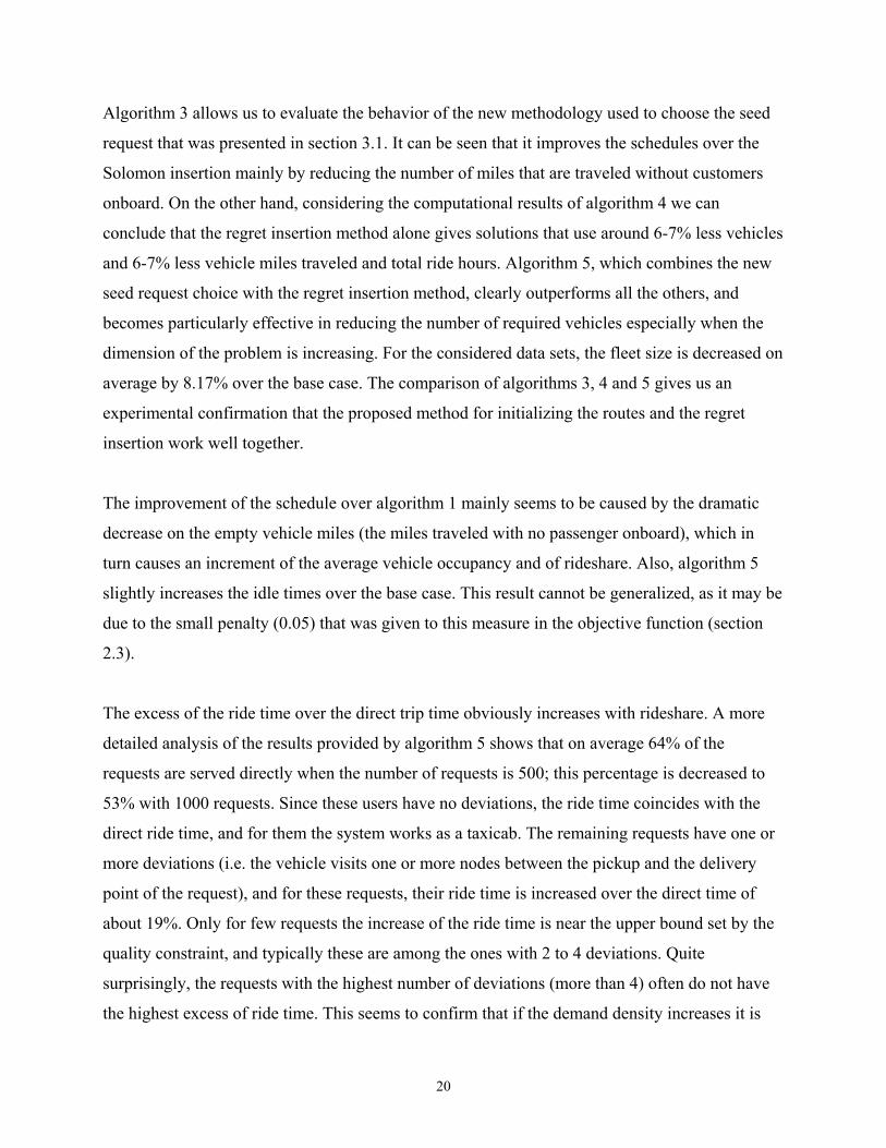
In figure 1, we illustrate how this computation is performed for both kinds of requests. Using this

definition for time windows, the number of tentative insertions that must be performed is

dramatically reduced by a priori discarding those that would be infeasible as regards to some of

these constraints. Unlike the definition proposed by Jaw et al. (1986), it can be seen that our time

windows also imply the respect of the maximum ride time. The most serious drawback is that the

time window related to the delivery point (for pickup-time specified requests) or to the pickup

point (for delivery-time specified requests) is to some extent unnecessarily narrowed, and this

could in turn make it more difficult to identify a feasible solution. On the other hand, narrowing

these time windows leads to solutions of high quality for the traveler. This aspect will be

investigated when we present the results of the computational tests.

Fig. 1.

In addition, we associate with each request k a service time sk both at the pickup and at the

delivery node. This service feature is usually considered only in the case of the design of a

paratransit system for disabled persons. In fact, when modeling a high quality service, in which

the temporal constraints are very tight, the length of operations such as boarding and paying the

fare cannot be overlooked.

2.2. Idle times within the schedule

As previously mentioned, we are dealing with a highly constrained problem. In order to enlarge

the solution space without affecting the quality of the service, the vehicles are allowed to stop and

idle at any pickup location, waiting to serve the following request, if only no passengers are

onboard. This modification of the standard dial-a-ride problem increases the possibility of

inserting new requests, especially when the time windows are narrow and the number of requests

per unit of time is low. Furthermore, on an operational point of view, the presence of these pauses

could greatly simplify the crew roster design, as a multitude of points in which a driver turnover

is possible, is created. On the other hand, the implementation of this possibility drives to a more

8

complicated algorithm design, as the insertion of new requests across an idle time might cause a

passenger to be onboard while the vehicle is idling.

The easiest method to avoid this drawback is to prevent the algorithm from performing insertions

of requests across one or more pauses. This limitation is somewhat arbitrary, as there could be the

possibility of operating a shift in the schedule in such a manner that the included idle times are

eliminated, thus making the insertion possible. Our algorithm performs this check, and in our

computational tests we measured to what extent this added capability improves the quality of the

solution (see section 4).

2.3. Objective function

When operating a public transport service there are always two conflicting points of view to be

considered. The service provider is interested in the economic efficiency of the system, whereas

the customer looks at the service quality. The objective function to minimize is a weighted sum

of three elements that represent these different points of view: (1) the total distance traveled by

all the vehicles, (2) the excess ride time over the direct time for all the customers and (3) the total

length of the idle times within the schedule. The latter can also not be considered if it is stated

that a vehicle can idle without passengers onboard at no cost. In our simulation we used 0.45,

0.55 and 0.05 as weights for the three components, not considering the scaling factors.

The number of vehicles to be used is not minimized during the optimization process; but it is an

input of the algorithm. To test the performance of the proposed heuristic, in our computational

tests we iteratively run each scenario to determine the minimum number of vehicles required to

service all the requests. In order to do this, we performed the first run of the algorithm with a very

high number of vehicles, and we progressively lowered this number in the successive runs until

some requests could not be scheduled.

3. The proposed regret insertion heuristic

9

From the discussion presented in the previous section we can conclude that the studied problem

is an extremely constrained problem, and therefore the feasibility region can be very limited,

even compared to the classical pickup and delivery problem with time windows. On the other

hand, from the point of view of the professional scheduler of a paratransit system, the quality of

the solution in terms of the minimization of the objective function might not be the only desired

feature. In an operative context, even if real-time requests are not allowed, there are always some

elements that make the problem dynamic (no shows, vehicle breakdowns…). Thus, it is also

useful to have a solution that allows some degree of flexibility. In other words, operating changes

in the current schedule, such as adding or removing requests or changing the travel times of some

arcs, should not always cause the schedule to become infeasible.

These considerations led us to develop a heuristic primarily focusing on the “maximization of the

feasibility” of the solution found. On the other hand, a considerable amount of past research

(Solomon, 1987) has shown that the insertion methods perform best when we face a routing

problem with time windows. Furthermore, Liu and Shen (1999) for example show that parallel

insertion procedures outperform sequential approaches. Our proposal is to adopt a parallel

insertion heuristic with an appropriate metric, aimed at improving the myopic behavior that is

often the drawback of such methods. The metric we use in our algorithm is the generalized regret

measure, a technique that has been already employed with interesting results for the study of the

standard vehicle routing problem with time windows (Potvin and Rousseau, 1993; Liu and Shen,

1999). The regret metric is particularly useful in finding feasible solutions for highly constrained

problems.

3.1. The seed request choice

Assuming there are m vehicles, the initial request to be serviced for each of the m tours needs to

be determined. Previous research has shown the sensitivity and the importance of the

initialization of the m tours of a parallel construction heuristic in order to obtain good solutions.

One of the simplest and most intuitive ways to initialize the routes is to choose the m requests

with the earliest pickup time. This initialization rule however does not keep into account the

routing aspect of the problem, and could perform poorly when solving instances in which the

10

requests are spread over the territory. In fact, it has been pointed out that in this situation the

farthest requests tend to be inserted last, and this behavior clearly worsens the final solution.

One way to overcome this flaw is to keep into account the spatial position of the requests when

making the choice of the seeds, trying to consider the ones that are more decentralized, as well as

the ones with the earliest pickup time. The underlying idea of this initialization strategy is

consistent with that of the regret insertion method that we will introduce later, since in both cases

we try to anticipate the insertion of a request that would be hard or not convenient to consider

later.

Different proposals can be found in the literature on the Vehicle Routing Problem for efficiently

choosing the seed requests. From the routing aspect, the most popular approaches are variants of

the one originally proposed by Fisher and Jaikumar (1981) that partitions the plane in m cones,

whose vertex are the central depot, and chooses the seed customers on the basis of their distance

from it. This idea is also used by many authors to determine in which order the request must be

inserted (Russell, 1995; Caseau and Laburthe, 1999), but in our case this is irrelevant, since the

insertion order is determined by the regret heuristic. For mixed routing and scheduling problems,

usually a ranking index is defined on the basis of two aspects. Russell (1995) takes into account

the temporal location and the length of the time windows along with the distance from the depot,

whereas Toth and Vigo (1997) propose a more elaborate methodology that considers the loading

and unloading times of the customers and the travel times from the pickup and delivery points of

the request under consideration to all the other nodes.

As our primary concern is to provide a high quality service, in our case the time windows are

quite narrow. Furthermore, we study the feasibility of paratransit systems in an urban

environment, where the density of requests could be relatively high. The combination of these

two factors makes the scheduling aspect of the problem preponderant on the routing, far beyond

the cases addressed in the cited studies. Hence, we basically keep the idea of ranking the requests

in ascending pickup time order, but we operate two major modifications. We try to avoid to

initialize a route with a request that can be easily inserted after a previously chosen seed, and we

11

allow some swaps in the ranking order to give preference to the requests that could be difficult to

insert later, due to their spatial position.

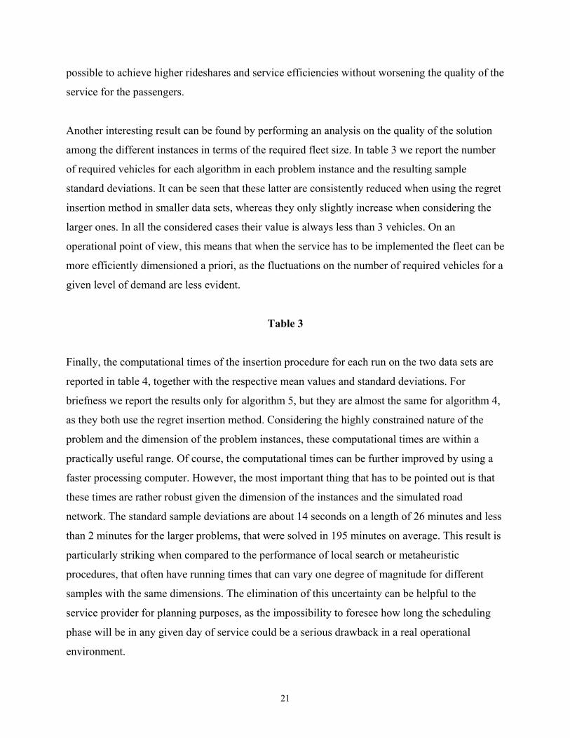
We illustrate our procedure through an example. In figure 2, we represent on a time line the

pickup (p) and delivery (d) points associated to the earliest five requests of a set; we omit to

represent the associated time windows for simplicity. We want to choose three seed requests

among these since we assume there are three vehicles, and again for simplicity we suppose that

the distance between any pair of nodes associated to these five requests is the same. According to

the earliest pickup time ranking, requests 1, 2, and 3 should be the initial requests. It can however

be seen that these three are much more spaced in terms of pickup and delivery times (and so a

vehicle could easily service all of them), whereas requests 3, 4 and 5 are so close in their pickup

and delivery times that they cannot be served by the same vehicle. As a consequence, it would be

more efficient to consider for example requests 1, 4 and 5 as seed candidates, as shown in the

figure. To take these cases into account, we consider each pair of consecutive requests k and k+1.

If the kth request has already been chosen as seed and if the following inequality is verified

1k1)P(kD(k),k EPTTTLDT ++ ≤+

then the (k+1)th request is not taken as seed, and we consider the kth and the (k+2)th requests. The

quantity TTD(k),P(k+1) is the travel time between the delivery point of request k and the pickup point

of the following, whereas LDTk is the latest delivery time of request k and EPTk+1 is the earliest

pickup time of request k+1, as defined by the associated time windows.

Fig. 2

We also try to consider the spatial aspect of the problem. To do this, we compute for each request

k a decentralization index (Dk) given by the following expression, in which TD represents the

travel distance between the specified pair of nodes and n is the total number of requests:

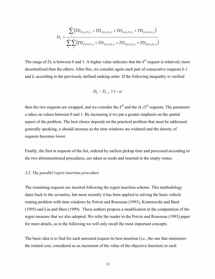
12

( )

( )∑∑

∑

+++

+++= n

k

n

jjDkDjPkDjDkPjPkP

n

jjDkDjPkDjDkPjPkP

k

TDTDTDTD

TDTDTDTDD

)(),()(),()(),()(),(

)(),()(),()(),()(),(

The range of Dk is between 0 and 1. A higher value indicates that the kth request is relatively more

decentralized than the others. After this, we consider again each pair of consecutive requests k-1

and k, according to the previously defined ranking order. If the following inequality is verified

α−≥− − 11kk DD

then the two requests are swapped, and we consider the kth and the (k-2)th requests. The parameter

α takes on values between 0 and 1. By increasing it we put a greater emphasis on the spatial

aspect of the problem. The best choice depends on the practical problem that must be addressed:

generally speaking, α should increase as the time windows are widened and the density of

requests becomes lower.

Finally, the first m requests of the list, ordered by earliest pickup time and processed according to

the two aforementioned procedures, are taken as seeds and inserted in the empty routes.

3.2. The parallel regret insertion procedure

The remaining requests are inserted following the regret insertion scheme. This methodology

dates back to the seventies, but more recently it has been applied to solving the basic vehicle

routing problem with time windows by Potvin and Rousseau (1993), Kontoravdis and Bard

(1995) and Liu and Shen (1999). These authors propose a modification in the computation of the

regret measure that we also adopted. We refer the reader to the Potvin and Rousseau (1993) paper

for more details, as in the following we will only recall the most important concepts.

The basic idea is to find for each unrouted request its best insertion (i.e., the one that minimizes

the related cost, considered as an increment of the value of the objective function) in each

13

itinerary. In this manner, we build an incremental cost matrix in which the rows represent the

requests and the columns the routes. If a request has no feasible insertion in a route, the

corresponding incremental cost is set to an arbitrarily large value. After that, we compute for each

request its regret, given by the sum of the differences between all the elements of the

corresponding row and the minimum one. The request with the largest regret will be inserted in

the previously computed position. These steps are iterated until all the requests are inserted or

until all the regret costs are zero. In the latter case, the corresponding requests cannot be inserted

in any of the existing routes.

The regret cost is a measure of the potential price that could be paid if a given request were not

immediately inserted. As it can be seen, whenever a request cannot be inserted in a route, the

related regret cost is greatly incremented. This feature is particularly useful for highly constrained

problems, as it drives the algorithm towards the search of feasible solutions. The main focus is to

limit as much as possible the myopic behavior of the classical insertion procedures, which for

mixed scheduling and routing problems with additional constraints is particularly harmful. In

summary, both the initialization and the insertion procedures have been designed to consistently

pursue the same goals.

3.3. Quickly checking the feasibility of an insertion

The regret insertion algorithm requires at each step to tentatively check the insertion of each

unrouted request (that is, both the pickup and the delivery point) in every feasible position of all

the vehicles. Its computational complexity is of O(n3). For this, it is even more important than for

classical insertion heuristics, whose computational complexity is usually O(n2), to develop

methods for rapidly checking the feasibility of the insertion of a request in a predetermined

position. The most difficult part is to control the deviation from the original route that is needed

to serve a customer without causing a violation of the time windows of any previously inserted

requests. Of course this is not a sufficient condition to have a feasible insertion, but it is the most

difficult one to check, and perhaps also the most important, as when modeling the problem we

incorporated in the time window definition the constraints related to both the scheduling of the

14

request and to the quality of the service. In the following we will not discuss the more trivial

checks related to the respect of the capacity and of the coupling constraints.

Jaw et al. (1986) perform the time windows control by decomposing each route in different

schedule blocks, defined by the corresponding time intervals in which the vehicle is serving

requests without idling. They then develop a procedure to check if the insertion of a request in a

schedule would cause a violation of the time windows of any previously inserted request within

the schedule block. To accomplish this task, four quantities are computed for each node i of the

schedule sequence: BUPi, BDOWNi, AUPi and ADOWNi, representing the maximum time interval

by which the nodes in the schedule block preceding and following i (i is included) can be pushed

backward and forward. If the additional time required to reach a point is larger than BUPi +

ADOWNi+1, then the insertion of this point between i and i+1 is not feasible, as it would cause

the violation of some time windows of the nodes in the schedule. We remark that associated with

each request k are two nodes, one representing the pickup point and the other representing the

delivery point.

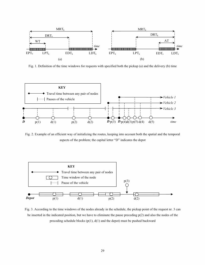
It can be seen that this procedure focuses only on the single schedule block. During the insertion

process, as more requests are inserted, the pauses between schedule blocks decrease. To prevent

two or more schedule blocks from overlapping, the above four measures are defined so that the

feasible shifts are bounded by the length of the idle times within them. This is an additional

constraint not required by the original problem, that could be removed if the shifts needed to

serve a request could propagate across different blocks. For example, in figure 3 we can see that

the pickup point of the request number 3 can be inserted between p(2) and d(2) only if we

eliminate the pause between the two blocks and allow the whole schedule to be pushed backward.

Fig. 3

Generally speaking, it would be nice to check the feasibility of the insertion of a node only on the

basis of the time windows of the entire route, automatically creating and merging the different

schedule blocks. This improvement is of great importance when we look for solutions of good

quality for the customers, as the average number of pauses per route grows when the time

15

windows are narrowed. Using the above mentioned technique would lead to a great difficulty in

inserting new requests, given by our feasibility check method and not implied in the problem

itself. In order to avoid this problem, in our algorithm we use different statistics, so that it is

possible to check in one step if the insertion of a pickup or delivery point causes some time

window violation over the entire schedule of the vehicle. For each node i we define four

quantities: BTOPi and BBOTTOMi (the maximum time interval by which i and all the preceding

nodes in the vehicle schedule can be pushed backward and forward, respectively), ATOPi and

ABOTTOMi (the maximum time interval by which i and all the following nodes in the vehicle

schedule can be pushed backward and forward, respectively). To understand how can we

mathematically define these statistics, let us focus our attention on a generic node i of a schedule

block h delimited by the idle times dsh and dsh+1.

If we consider the quantity BBOTTOMi, it is evident that it is not influenced by the time windows

of the nodes preceding dsh, as a forward shift of the nodes between dsh and i can simply be

compensated by increasing dsh of the corresponding quantity. The same happens with ATOPi.

The time windows only within the same schedule blocks must be considered. In summary, the

definition of BBOTTOMi and ATOPi is the same as the one for BDOWNi and AUPi as proposed

by Jaw et al. (1986). We report it in the following recursive form.

In the preceding equations we indicated with ATi the leaving time currently scheduled for the

node i after that the service has been exploited, whereas ETi and LTi are the earliest and latest

scheduled time given by the associated time window and si is the needed service time.

Let us now consider BTOPi. It is evident that this quantity is influenced by the time windows of

all the preceding nodes of the schedule, as well by all the preceding pauses. In the same manner,

−−−−

=+ otherwise)ETsAT,(ATOPmin

block scheduleeach of nodefirst for the ETsAT ATOP

iii1i

iiii

−−

=− otherwise)ATLT,(BBOTTOMmin

block scheduleeach of nodelast for the ATLTBBOTTOM

ii1i

iii

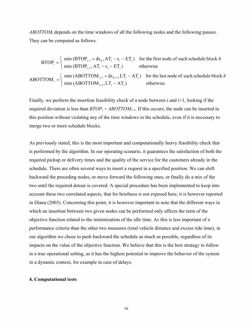
16

ABOTTOMi depends on the time windows of all the following nodes and the following pauses.

They can be computed as follows.

Finally, we perform the insertion feasibility check of a node between i and i+1, looking if the

required deviation is less than BTOPi + ABOTTOMi+1. If this occurs, the node can be inserted in

this position without violating any of the time windows in the schedule, even if it is necessary to

merge two or more schedule blocks.

As previously stated, this is the most important and computationally heavy feasibility check that

is performed by the algorithm. In our operating scenario, it guarantees the satisfaction of both the

required pickup or delivery times and the quality of the service for the customers already in the

schedule. There are often several ways to insert a request in a specified position. We can shift

backward the preceding nodes, or move forward the following ones, or finally do a mix of the

two until the required detour is covered. A special procedure has been implemented to keep into

account these two correlated aspects, that for briefness is not exposed here; it is however reported

in Diana (2003). Concerning this point, it is however important to note that the different ways in

which an insertion between two given nodes can be performed only affects the term of the

objective function related to the minimization of the idle time. As this is less important of a

performance criteria than the other two measures (total vehicle distance and excess ride time), in

our algorithm we chose to push backward the schedule as much as possible, regardless of its

impacts on the value of the objective function. We believe that this is the best strategy to follow

in a true operational setting, as it has the highest potential to improve the behavior of the system

in a dynamic context, for example in case of delays.

4. Computational tests

−−−−+

=−

−

otherwise)ETsAT,(BTOPmin block scheduleeach of nodefirst for the)ETsAT,ds(BTOPmin

BTOPii1i

iih1ii

i

i h

−−+

=+

++

otherwise)ATLT,(ABOTTOMmin block scheduleeach of nodelast for the)ATLT,ds(ABOTTOMmin

ABOTTOMi1i

ii1h1ii

i

h

17

4.1. Generating random samples

The algorithm presented in section 3 has been tested simulating a realistic dial-a-ride system with

data provided by Access Services, Inc. (ASI). ASI is the transit agency designated to coordinate

paratransit services for elderly and disabled persons within Los Angeles County. About 6000

requests, spread on a territory of more than 10,500 square kilometers, are served each weekday

through various providers, each one operating in a different region of the County. The average

daily number of requests serviced by each provider depends on the region and varies from 250 to

2000 requests per day. By performing a statistical analysis of the data provided by ASI over a

three-day period of service operation, Dessouky and Adam (1998) suggest techniques for

generating random samples that are representative of the possible service requests both in spatial

and in temporal terms; the interested reader is referred to that work for more details, as in the

following we will only recall the main steps. We determined the coordinates (x,y) of the pickup

location of each request by dividing the service area in 15 bins of 10x10 miles giving a total

service area of 150x150 miles. In order to represent clusters that are exhibited in the actual data,

the probability a request is within each bin is not uniform. The distribution of the requests in the

different bins was statistically induced from the real data, and then samples were drawn to

determine in which bin each pickup point is located. After determining the bin, two samples were

drawn from a uniform (-5,5) distribution to determine the coordinates (x,y). The delivery point

was selected by adding to the pickup point the travel length, which was sampled from the

distribution of the travel lengths. The direction of addition to determine the delivery point was

sampled from a uniform (0, 2π) distribution.

The distribution from which the pickup times of the samples were drawn were based on the

empirical distributions derived from Los Angeles County (see Dessouky and Adam, 1998). After

that, the delivery times were determined on the basis of the travel distance assuming a constant

speed of travel (20 mph).

The service times at the nodes, expressed in minutes, were drawn from a uniform (1,3)

distribution for passengers with wheelchair and were fixed to 30 seconds for the other requests.

The probability to serve a passenger with a wheelchair was set to 0.20, and the number of

18

accompanying passengers was obtained as a sample of the following cumulative distribution: 0-

0.40; 1-0.99; 2-1.00. For requests without passengers on a wheelchair, the probability of having

two people to transport was 0.175. The remaining requests travel alone. All these assumptions are

based on the analysis of the ASI data reported by Dessouky and Adam (1998).

We generated two distinct sets of problem instances, each one having five random samples. In the

first set all the samples contain 500 requests, in the second 1000 requests. For each scenario, we

simulate 24 hours of provided service. These parameters represent a fairly large-scale instance of

this kind of system.

4.2. Implementation of the algorithm and computational results

According to the problem definition that we introduced in section 2, we need to specify some

parameters that assure an acceptable quality of service for all the customers. As our final aim is to

check if dial-a-ride services can be feasible also for the general public, we were particularly

restrictive in the selection of the parameters related to the quality of the service. For this, we fixed

the time window span to 10 minutes, in order to make the average waiting time similar to a

typical transit line, and we imposed that the maximum ride time for each request must not exceed

1.3 times the direct ride time plus 10 minutes. Note that within these time windows the above

defined service times must be comprised, so that, for example, a service time of 2 minutes in a

time window of 10 reduces the feasible shift of the schedule to 8 minutes. In section 4.3 we will

present the results of a sensitivity analysis on the tightness of the scheduling constraints.

In order to realize if our methodology performs better than other possible approaches, we

implemented five different variants and we tested them on the same problem instances. In

algorithm 1 the seed requests are chosen exclusively on the basis of the pickup time and a parallel

version of the classical Solomon sequential insertion is performed (Solomon, 1987). Thus, the

request to be inserted is the one that causes the least increment of the value of the objective

function. Algorithm 2 is very similar to algorithm 1, but the insertion of a request across different

schedule blocks is also allowed, according to the description in section 3.3. As mentioned in Jaw

et al. (1986), whose heuristic does not provide for this capability, from a conceptual point of view

19

this should allow for a better exploration of the feasibility region of the problem, thus, improving

the quality of the solution found. Algorithm 3 uses the seed request choice procedure described in

section 3.1, but performs the Solomon insertion. Algorithm 4 initializes the routes like algorithms

1 and 2, but the regret insertion is performed. Finally, algorithm 5 represents our proposal, as it

uses both the new seed request choice and the regret insertion. All these algorithms were coded in

C++ and executed on a Personal Computer with a Pentium® III processor.

The implementation of all these variants allows us to see the effective behavior of each

alternative, compared to the classical base case represented by algorithm 1. The computational

results for the sets of 500 requests and of 1000 requests are shown in tables 1 and 2, respectively.

The reported numbers refer to the mean values obtained from independent runs on five different

random samples, as earlier described. Each table reports the following information: the first

column indicates the used algorithm and the second the minimum number of vehicles needed to

serve all the requests. After that, the overall number of miles that are covered and the miles that

are traveled with no passengers onboard (excluding the trips to and from the depot) are shown.

The fifth and the sixth columns contain the total length of the schedule, i.e. the sum of the time

intervals from leaving to returning to the depot of all the vehicles, and the total length of all the

idle times. Finally, we report a rideshare measure, i.e. the ratio between the number of served

requests and the number of trips started with no passengers onboard, and the average increase of

the ride time as regards to the direct ride time.

Tables 1 and 2

Several comments are possible on the basis of these data. Algorithms 1 and 2 perform almost the

same when solving problems with 500 requests, whereas there is an improvement of the latter for

the bigger instances, moreover if we consider the number of vehicles needed. In those cases

algorithm 2 has a slightly better performance, although on an intuitive point of view the

possibility of inserting requests across different schedule blocks should have had a much deeper

impact. A possible explanation is that it is likely that eliminating the pauses leads to a less

flexible schedule, that in turn worsens the quality of the insertion for the later requests.

20

Algorithm 3 allows us to evaluate the behavior of the new methodology used to choose the seed

request that was presented in section 3.1. It can be seen that it improves the schedules over the

Solomon insertion mainly by reducing the number of miles that are traveled without customers

onboard. On the other hand, considering the computational results of algorithm 4 we can

conclude that the regret insertion method alone gives solutions that use around 6-7% less vehicles

and 6-7% less vehicle miles traveled and total ride hours. Algorithm 5, which combines the new

seed request choice with the regret insertion method, clearly outperforms all the others, and

becomes particularly effective in reducing the number of required vehicles especially when the

dimension of the problem is increasing. For the considered data sets, the fleet size is decreased on

average by 8.17% over the base case. The comparison of algorithms 3, 4 and 5 gives us an

experimental confirmation that the proposed method for initializing the routes and the regret

insertion work well together.

The improvement of the schedule over algorithm 1 mainly seems to be caused by the dramatic

decrease on the empty vehicle miles (the miles traveled with no passenger onboard), which in

turn causes an increment of the average vehicle occupancy and of rideshare. Also, algorithm 5

slightly increases the idle times over the base case. This result cannot be generalized, as it may be

due to the small penalty (0.05) that was given to this measure in the objective function (section

2.3).

The excess of the ride time over the direct trip time obviously increases with rideshare. A more

detailed analysis of the results provided by algorithm 5 shows that on average 64% of the

requests are served directly when the number of requests is 500; this percentage is decreased to

53% with 1000 requests. Since these users have no deviations, the ride time coincides with the

direct ride time, and for them the system works as a taxicab. The remaining requests have one or

more deviations (i.e. the vehicle visits one or more nodes between the pickup and the delivery

point of the request), and for these requests, their ride time is increased over the direct time of

about 19%. Only for few requests the increase of the ride time is near the upper bound set by the

quality constraint, and typically these are among the ones with 2 to 4 deviations. Quite

surprisingly, the requests with the highest number of deviations (more than 4) often do not have

the highest excess of ride time. This seems to confirm that if the demand density increases it is

21

possible to achieve higher rideshares and service efficiencies without worsening the quality of the

service for the passengers.

Another interesting result can be found by performing an analysis on the quality of the solution

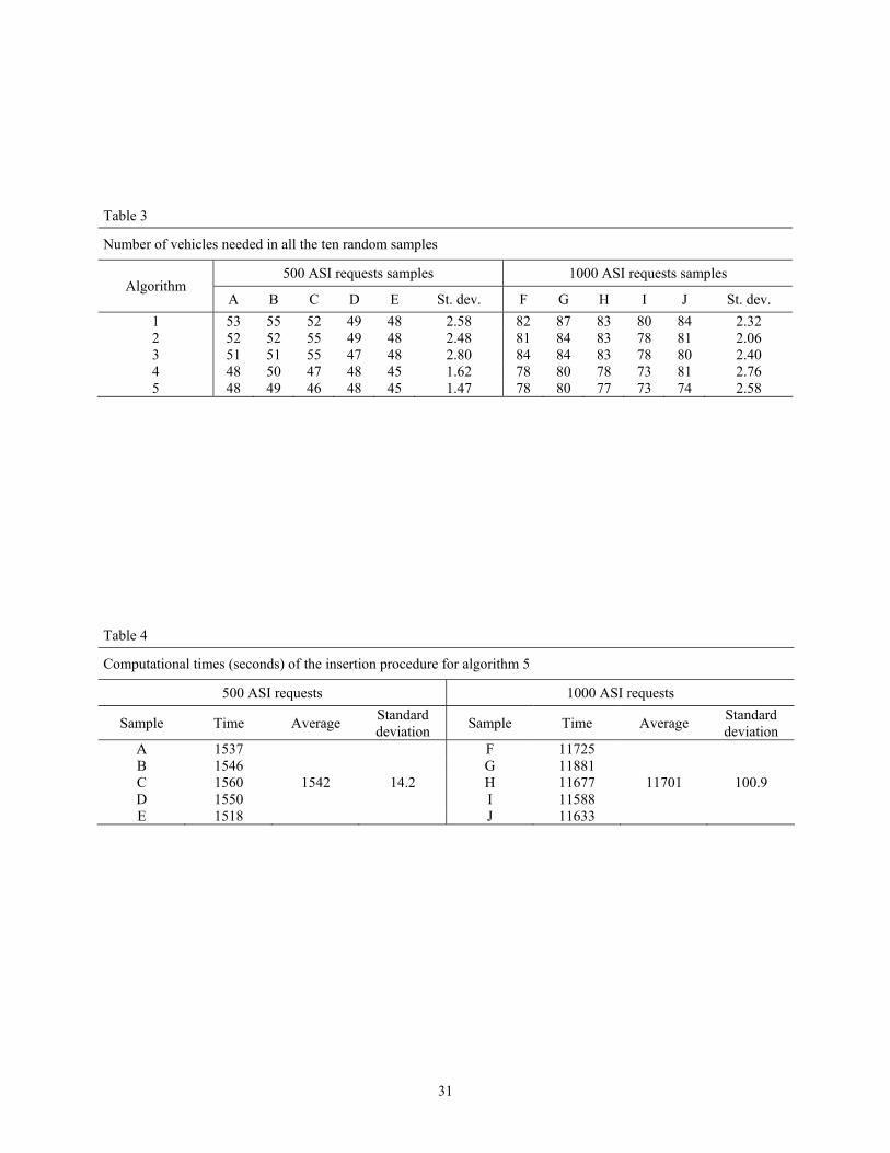
among the different instances in terms of the required fleet size. In table 3 we report the number

of required vehicles for each algorithm in each problem instance and the resulting sample

standard deviations. It can be seen that these latter are consistently reduced when using the regret

insertion method in smaller data sets, whereas they only slightly increase when considering the

larger ones. In all the considered cases their value is always less than 3 vehicles. On an

operational point of view, this means that when the service has to be implemented the fleet can be

more efficiently dimensioned a priori, as the fluctuations on the number of required vehicles for a

given level of demand are less evident.

Table 3

Finally, the computational times of the insertion procedure for each run on the two data sets are

reported in table 4, together with the respective mean values and standard deviations. For

briefness we report the results only for algorithm 5, but they are almost the same for algorithm 4,

as they both use the regret insertion method. Considering the highly constrained nature of the

problem and the dimension of the problem instances, these computational times are within a

practically useful range. Of course, the computational times can be further improved by using a

faster processing computer. However, the most important thing that has to be pointed out is that

these times are rather robust given the dimension of the instances and the simulated road

network. The standard sample deviations are about 14 seconds on a length of 26 minutes and less

than 2 minutes for the larger problems, that were solved in 195 minutes on average. This result is

particularly striking when compared to the performance of local search or metaheuristic

procedures, that often have running times that can vary one degree of magnitude for different

samples with the same dimensions. The elimination of this uncertainty can be helpful to the

service provider for planning purposes, as the impossibility to foresee how long the scheduling

phase will be in any given day of service could be a serious drawback in a real operational

environment.

22

Table 4

4.3. Sensitivity analysis on the tightness of the scheduling constraints

As we mentioned in section 2.3, in a DRT system the interests of the customers and of the service

provider are contrasting. Hence, it is essential for its success to find the right balance between

these opposing points of view. This can be done by investigating the relationship between the

increase of the service quality and the corresponding increase of operating costs. Thus, it is

interesting to evaluate the behavior of the proposed heuristic also under different operating

scenarios.

In order to do this, we solved again the five larger problems, involving 1000 requests, under

different conditions. We defined three scenarios beyond the one studied in the preceding section,

each of these being characterized by a certain minimum time window span and maximum ride

time. We report in table 5 the settings that have been used. Scenario “L” has characteristics that

are similar to a typical paratransit service for disabled people, whereas the quality of scenario

“H” can be comparable to that of a taxicab, except for the possibility of ridesharing.

Table 5

We focus our attention on variants 1 and 5 of our algorithm, representing respectively the

standard solution method and our new proposal. For these, the mean computational results over

the five samples for the defined scenarios are reported in table 6. It can be seen that algorithm 5

improves over algorithm 1 in all the considered scenarios. However, the regret insertion

algorithm performs best against the classical insertion heuristic under medium to small time

window constraints. When the time window is large, the benefit of the regret procedure is

reduced. When the time window is very small (scenario “H”), the gap between the regret

insertion and algorithm 1 also narrows since in this case the number of feasible alternatives is

rather small. Thus, there are few feasible insertion scheduling alternatives to consider.

23

Table 6

5. Conclusions

In this paper we presented a new heuristic designed to solve large problem instances of a realistic

formulation of the dial-a-ride problem with time windows. The heuristic was tested on a series of

instances that were built from data concerning three days of paratransit operation in Los Angeles

County. The results of these experiments showed that the quality of the solution is consistently

improved with respect to a classical insertion heuristic.

Our efforts were directed at finding a good balance between the need of developing a tool that

could be used in practice, the quality of the solution and the associated computational burden of

the heuristic. The regret insertion scheme furthermore does not have parameters to be set, which

is in contrast to local search and metaheuristic procedures. Our heuristic can manage instances of

big dimensions for the studied problem. If we compare the outputs for the two data sets, it is

evident that bigger instances are harder to solve, but in turn the proposed heuristic considerably

outperforms the classical insertion heuristic for the large problem instances. On the other hand,

preliminary experiments with only 100 requests showed no significant differences between the

two approaches in terms of the quality of the solution.

The feasibility of the implementation of a demand-responsive transit system for the general

population is currently under consideration in the city of Turin (Italy), as an advanced Intelligent

Transport System is already in use both for traffic management and for the operation of the

public transport lines. Research work is in progress on the topic, but the need of a reliable

algorithm for the operation of the service is one of the primary concerns. The next phase of our

research will be targeted at adapting the scheduling capabilities of the presented algorithm to this

transit environment, including the possibility of inserting real-time requests.

Acknowledgements

24

This research was made possible by a grant from the Turin Transit Agency ATM (Azienda

Torinese per la Mobilità), Italy. Dr. Dessouky’s time was supported by the National Science

Foundation under grant DMI-9732878. Thanks are also due to Access Services, Inc. for

providing the data upon which the problem instances were built. We also wish to acknowledge

the comments of an anonymous referee that were helpful in improving the quality of this paper.

References

Bodin, L. and Sexton, T. (1986) The multi-vehicle subscriber dial-a-ride problem. TIMS Studies

in the Management Sciences, 22, 73-86.

Borndörfer, R., Grötschel, M., Klosteimer, F. and Küttner, C. (1999) Telebus Berlin: vehicle

scheduling in a dial-a-ride system. Lecture Notes in Economics and Mathematical Systems

471: Computer-Aided Transit Scheduling. Springer-Verlag, Berlin, 391-422.

Caseau, Y. and Laburthe, F. (1999) Heuristics for large constrained vehicle routing problems.

Journal of Heuristics, 5, 281-303.

Cervero, R. (1997) Paratransit in America – Redefining mass transportation. Praeger, Westport.

Daganzo, C. (1978) An approximate analytic model of many-to-many demand responsive

transportation systems. Transportation Research, 12, 325-333.

Desaulniers, G., Desrosiers, J., Erdmann, A., Solomon, M.M. and Soumis, F. (2000) The VRP

with pickup and delivery. Cahiers du GERAD G-2000-25, Ecole des Hautes Etudes

Commerciales, Montréal.

Desrosiers, J., Dumas, Y. and Soumis, F. (1986) A dynamic programming solution of the large-

scale single-vehicle dial-a-ride problem with time windows. American Journal of

Mathematical and Management Sciences, 6, 301-325.

Desrosiers, J., Dumas, Y. and Soumis, F. (1988) The multiple dial-a-ride problem. Lecture Notes

in Economics and Mathematical Systems 308: Computer-Aided Transit Scheduling. Springer,

Berlin.

Dessouky, M. and Adam, S. (1998) Real-time scheduling of demand responsive transit service -

Final report. University of Southern California, Department of Industrial and Systems

Engineering, Los Angeles.

25

Dial, R.B. (1995) Autonomous Dial-a-Ride Transit: introductory overview. Transportation

Research C, 3C, 261-275.

Diana, M. (2003) Methodologies for the tactical and strategic design of large-scale advance-

request and real-time demand responsive transit services, Ph.D. Dissertation, Politecnico di

Torino, Dipartimento di Idraulica, Trasporti e Infrastrutture Civili, Torino, Italy.

Dumas, Y., Desrosiers, J. and Soumis, F. (1991) The pickup and delivery problem with time

windows. European Journal of Operational Research, 54, 7-22.

Fisher, M.L. and Jaikumar, R. (1981) A generalized assignment heuristic for vehicle routing.

Networks, 11, 109-124.

Fu, L. (2002) A simulation model for evaluating advanced dial-a-ride paratransit systems.

Transportation Research A, 36A, 291-307.

Healy, P. and Moll, R. (1995) A new extension of local search applied to the dial-a-ride problem.

European Journal of Operational Research, 83, 83-104

Horn, M.E.T. (2002a) Multi-modal and demand-responsive passenger transport systems: a

modelling framework with embedded control systems. Transportation Research A, 36A, 167-

188.

Horn, M.E.T. (2002b) Fleet scheduling and dispatching for demand-responsive passenger

services. Transportation Research C, 10C, 35-63.

Ioachim, I., Desrosiers, J., Dumas, Y., Solomon, M.M. and Villeneuve, D. (1995) A request

clustering algorithm for door-to-door handicapped transportation. Transportation Science, 29,

63-78.

Jaw, J.J., Odoni, A.R., Psaraftis, H.N. and Wilson, N.H.M. (1986) A heuristic algorithm for the

multi-vehicle many-to-many advance request dial-a-ride problem. Transportation Research B,

20B, 243-257.

Kontoravdis, G. and Bard, J.F. (1995) A GRASP for the vehicle routing and scheduling problem

with time windows. ORSA Journal of Computing, 7, 10-23.

Lave, R.E., Teal, R. and Piras, P. (1996) A handbook for acquiring demand-responsive transit

software, Transit Cooperative Research Program Report #18, Transportation Research Board,

Washington, D. C.

Liu, F.H. and Shen, S.Y. (1999) A route-neighborhood-based metaheuristic for vehicle routing

problem with time windows. European Journal of Operational Research, 118, 485-504.

26

Lu, Q. and Dessouky, M. (2003) An exact algorithm for the multiple vehicle pickup and delivery

problem. Transportation Science, forthcoming.

Madsen, O.B.G., Raven, H.F. and Rygaard, J.M. (1995) A heuristic algorithm for a dial-a-ride

problem with time windows, multiple capacities, and multiple objectives. Annals of

Operations Research, 60, 193-208.

Min, H. (1989) The multiple vehicle routing problem with simultaneous delivery and pick-up

points. Transportation Research A, 23A, 377-386.

Nanry, W.P. and Barnes, J.W. (2000) Solving the pickup and delivery problem with time

windows using reactive tabu search. Transportation Research B, 34B, 107-121.

Potvin, J.Y. and Rousseau, J.M. (1993) A parallel route building algorithm for the vehicle routing

and scheduling problem with time windows. European Journal of Operational Research, 66,

1993, 331-340.

Psaraftis, H.N. (1980) A dynamic programming solution to the single vehicle many-to-many

immediate request dial-a-ride problem. Transportation Science, 14, 130-154.

Psaraftis, H.N. (1983a) An exact algorithm for the single vehicle many-to-many dial-a-ride

problem with time windows. Transportation Science, 17, 351-357.

Psaraftis, H.N. (1983b) k-interchange procedures for local search in a precedence-constrained

routing problem. European Journal of Operational Research, 13, 391-402.

Psaraftis, H.N. (1983c) Analysis of an O(N2) heuristic for the single vehicle many-to-many

euclidean dial-a-ride problem. Transportation Research B, 17B, 133-145.

Psaraftis, H.N. (1986) Scheduling large-scale advance-request dial-a-ride systems. American

Journal of Mathematical and Management Sciences, 6, 327-367.

Ruland, K.S. and Rodin, E.Y. (1997) The pickup and delivery problem: faces and branch-and-cut

algorithm. Computers and Mathematics with Applications, 33, 1-13.

Russell, R.A. (1995) Hybrid heuristics for the vehicle routing problem with time windows.

Transportation Science, 29, 156-166.

Savelsbergh, M.W.P. and Sol, M. (1995) The general pickup and delivery problem.

Transportation Science, 29, 17-29.

Savelsbergh, M.W.P. and Sol, M. (1998) DRIVE: dynamic routing of independent vehicles.

Operations Research, 46, 474-490.

27

Sexton, T.R. and Bodin, L.D. (1985a) Optimizing single vehicle many-to-many operations with

desired delivery times: 1. Scheduling. Transportation Science, 19, 378-410.

Sexton, T.R. and Bodin, L.D. (1985b) Optimizing single vehicle many-to-many operations with

desired delivery times: 2. Routing. Transportation Science, 19, 411-435.

Sexton, T.R. and Choi, Y. (1986) Pickup and delivery of partial loads with soft time windows.

American Journal of Mathematical and Management Sciences, 6, 369-398.

Solomon, M.M. (1987) Algorithms for the vehicle routing and scheduling problems with time

windows constraints. Operations Research, 35, 254-265.

Stein, D.M. (1978a) Scheduling dial-a-ride transportation problems. Transportation Science, 12,

232-249.

Stein, D.M. (1978b) An asymptotic probabilistic analysis of a routing problem. Mathematics of

Operations Research, 3, 89-101.

Teodorovich, D. and Radivojevic, G. (2000) A fuzzy logic approach to dynamic dial-a-ride

problem. Fuzzy Sets and Systems, 116, 23-33.

Toth, P. and Vigo, D. (1997) Heuristic algorithms for the Handicapped Persons Transportation

Problem. Transportation Science, 31, 60-71.

Van Der Bruggen, L.J.J., Lenstra, J.K. and Schuur, P.C. (1993) Variable-depth search for the

single-vehicle pickup and delivery problem with time windows. Transportation Science, 27,

298-311.

28

List of figures

Fig. 1. Definition of the time windows for requests with specified both the pickup (a) and the

delivery (b) time

Fig. 2. Example of an efficient way of initializing the routes, keeping into account both the

spatial and the temporal aspects of the problem; the capital letter “D” indicates the depot

Fig. 3. According to the time windows of the nodes already in the schedule, the pickup point of

the request nr. 3 can be inserted in the indicated position, but we have to eliminate the pause

preceding p(2) and also the nodes of the preceding schedule blocks (p(1), d(1) and the depot)

must be pushed backward

List of tables

Table 1. Computational results for the five algorithms, 500 ASI requests, average values on five

random samples

Table 2. Computational results for the five algorithms, 1000 ASI requests, average values on five

random samples

Table 3. Number of vehicles needed in all the ten random samples

Table 4. Computational times in seconds for algorithm 5

Table 5. Parameters settings for the studied scenarios

Table 6. Computational results of algorithms 1 and 5 for the three scenarios, 1000 ASI requests,

average values on five random samples

29

Fig. 1. Definition of the time windows for requests with specified both the pickup (a) and the delivery (b) time

Fig. 2. Example of an efficient way of initializing the routes, keeping into account both the spatial and the temporal

aspects of the problem; the capital letter “D” indicates the depot

Fig. 3. According to the time windows of the nodes already in the schedule, the pickup point of the request nr. 3 can

be inserted in the indicated position, but we have to eliminate the pause preceding p(2) and also the nodes of the

preceding schedule blocks (p(1), d(1) and the depot) must be pushed backward

p(1) d(1) p(3) p(2) p(4) d(4) p(5) d(5) d(2) time

Travel time between any pair of nodes Vehicle 1 Vehicle 2

Vehicle 3

DD D d(3)

Pauses of the vehicle

KEY

(a)

WT time

MRTk

DRTk

(b)

AT time

MRTk

DRTk

EPTk LPTk EDTk LDTk EPTk LPTk EDTk LDTk

p(1) d(1) p(2) d(2)

Time window of the node

Depot

p(3)Pause of the vehicle

Travel time between any pair of nodes

KEY

30

Table 1

Computational results for the five algorithms, 500 ASI requests, average values on five random samples

Algorithm Vehicles Total Miles Empty miles Ride hours Idle hours Rideshare Increase of ride time

1 51.4 10575 2985 739.75 263.28 1.223 6.89% 2 51.2

(-0.39%) 10496

(-0.75%) 2928

(-1.91%) 734.25

(-0.74%) 263.37

(+0.03%) 1.370

(+0.147) 9.31%

(+2.42%) 3 50.4

(-1.95%) 10492

(+0.78%) 2753

(-7.77%) 733.86

(-0.82%) 270.35

(+2.69%) 1.368

(+0.145) 9.29%

(+2.40%) 4 47.6

(-7.39%) 9840

(-6.95%) 2414

(-19.13%) 690.22

(-6.70%) 264.52

(+0.47%) 1.356

(+0.133) 9.13%

(+2.24%) 5 47.2

(-8.17%) 10027

(-5.18%) 2371

(-20.57%) 702.78

(-5.00%) 264.31

(+0.39%) 1.365

(+0.142) 9.37%

(+2.48%)

Table 2

Computational results for the five algorithms, 1000 ASI requests, average values on five random samples

Algorithm Vehicles Total Miles Empty miles Ride hours Idle hours Rideshare Increase of ride time

1 83.2 17818 4716 1254.17 401.21 1.373 9.64% 2 81.4

(-2.16%) 17661

(-0.88%) 4652

(-1.36%) 1242.88 (-0.90%)

391.75 (-2.36%)

1.583 (+0.210)

11.83% (+2.19%)

3 81.8 (-1.68%)

17748 (-0.39%)

4531 (-3.92%)

1248.79 (-0.43%)

407.49 (+1.57%)

1.585 (+0.212)

11.73% (+2.39%)

4 78.0 (-6.25%)

16642 (-6.60%)

3759 (-20.29%)

1174.18 (-6.38%)

405.38 (+1.04%)

1.570 (+0.197)

11.85% (+2.21%)

5 76.4 (-8.17%)

16643 (-6.59%)

3557 (-24.58%)

1178.82 (-6.01%)

414.41 (+3.29%)

1.583 (+0.210)

12.02% (+2.38%)

31

Table 3

Number of vehicles needed in all the ten random samples

500 ASI requests samples 1000 ASI requests samples Algorithm

A B C D E St. dev. F G H I J St. dev. 1 53 55 52 49 48 2.58 82 87 83 80 84 2.32 2 52 52 55 49 48 2.48 81 84 83 78 81 2.06 3 51 51 55 47 48 2.80 84 84 83 78 80 2.40 4 48 50 47 48 45 1.62 78 80 78 73 81 2.76 5 48 49 46 48 45 1.47 78 80 77 73 74 2.58

Table 4

Computational times (seconds) of the insertion procedure for algorithm 5

500 ASI requests 1000 ASI requests

Sample Time Average Standard deviation Sample Time Average Standard

deviation A 1537 F 11725 B 1546 G 11881 C 1560 1542 14.2 H 11677 11701 100.9 D 1550 I 11588 E 1518 J 11633

32

Table 5.

Parameters settings for the studied scenarios

Scenario Base (Section 4.2)

L (Low quality)

M (Medium quality)

H (High quality)

Slope of the linear equation for MRT

1.3 2.0 1.5 1.2

Constant term intercept of the linear equation

for MRT

10 20 10 5

Minimum time windows span 10 30 15 5

Table 6.

Computational results of algorithms 1 and 5 for the three scenarios, 1000 ASI requests, average values on five random samples

Scenario L M H1

Algorithm 1 5 1 5 1 5 Vehicles 63.2 58.4

(-7.59%) 77.2 70.0

(-9.33%) 92.8 87.2

(-6.03%) Total Miles 14712 13877

(-5.68%) 16663 15554

(-6.66%) 19152 18107

(-5.46%) Empty miles 3341 2153

(-35.56%) 4238 3061

(-27.77%) 5175 4122

(-20.35%) Ride hours 1044.85 987.63

(-5.48%) 1177.19 1101.82

(-6.40%) 1344.26 1273.77

(-5.24%) Idle hours 288.07 301.17

(+4.55%) 350.17 373.65

(+6.71%) 463.97 485.24

(+4.58%) Rideshare 2.305 3.037

(+0.732) 1.609 1.883

(+0.274) 1.152 1.225

(+0.073) Increase of ride time

39.54% 47.62% (+8.08%)

17.29% 20.38% (+3.09%)

3.43% 4.24% (+0.81%)

1 In one of the five samples there are two requests that cannot be scheduled with such tight constraints, since the sum of the direct ride time and of the service times at nodes exceeds their respective maximum ride time. Hence, they have not been considered.