a new probabilistic approach in rank regression with optimal

Journal of Machine Learning Research 8 (2007) 2727-2754 Submitted 1/07; Revised 7/07; Published 12/07

A New Probabilistic Approach in Rank Regression with OptimalBayesian Partitioning

Carine Hue [email protected]

Marc Boulle [email protected]

France Telecom R&D2, avenue Pierre Marzin22307 Lannion cedex, France

Editors: Isabelle Guyon and Amir Saffari

Abstract

In this paper, we consider the supervised learning task which consists in predicting the normalizedrank of a numerical variable. We introduce a novel probabilistic approach to estimate the posteriordistribution of the target rank conditionally to the predictors. We turn this learning task into a modelselection problem. For that, we define a 2D partitioning family obtained by discretizing numericalvariables and grouping categorical ones and we derive an analytical criterion to select the partitionwith the highest posterior probability. We show how these partitions can be used to build univariatepredictors and multivariate ones under a naive Bayes assumption.

We also propose a new evaluation criterion for probabilistic rank estimators. Based on thelogarithmic score, we show that such criterion presents the advantage to be minored, which is notthe case of the logarithmic score computed for probabilistic value estimator.

A first set of experimentations on synthetic data shows the good properties of the proposedcriterion and of our partitioning approach. A second set of experimentations on real data showscompetitive performance of the univariate and selective naive Bayes rank estimators projected onthe value range compared to methods submitted to a recent challenge on probabilistic metric re-gression tasks.

Our approach is applicable for all regression problems with categorical or numerical predictors.It is particularly interesting for those with a high number of predictors as it automatically detectsthe variables which contain predictive information. It builds pertinent predictors of the normalizedrank of the numerical target from one or several predictors. As the criteria selection is regularizedby the presence of a prior and a posterior term, it does not suffer from overfitting.

Keywords: rank regression, probabilistic approach, 2D partitioning, non parametric estimation,Bayesian model selection

1. Introduction

In this introduction, we precise the supervised learning task we address in this paper, that is the rankregression. We then show the interest of probabilistic learning approaches compared to deterministicones. Finally, we outline our contribution which aims at selecting a probabilistic predictive modelfor the rank of a numerical target with a nonparametric Bayesian approach.

c©2007 Carine Hue and Marc Boulle.

HUE AND BOULLE

1.1 Value, Ordinal and Rank Regression

In supervised learning, classification tasks, where the target variable is categorical, are usually dis-tinguished from regression tasks, where it is numerical. A less known task is the case where thetarget variable is ordinal, usually called ordinal regression (see Chu and Ghahramani, 2005, for astate of the art). In this case, there is a total order between the target values but no distance infor-mation. The practical problems studied in the machine learning community consider a low numberof distinct integer ranks, roughly 5 or 10, fixed before the learning. The aim is then to predict theright quintile or decile an example belongs to. The algorithms are generally evaluated with the meanzero-one error or with the mean absolute error obtained by considering the ordinal scales as consec-utive integers. Among the proposed methods, the principle of empirical risk minimization with aloss function measuring the probability of misclassification is applied by Herbrich et al. (2000), anonline algorithm based on the perceptron algorithm is proposed in the work of Crammer and Singer(2001), support vector machines are used by Shashua and Levin (2002) and Chu and Keerthi (2005)and Gaussian processes by Chu and Ghahramani (2005).

The choice of a low number of distinct ranks is generally motivated by simplicity reasons.However, this predefined target discretization can separate values which form a pertinent predictioninterval.

In this paper, we address rank regression tasks. More precisely, for a given numerical targetvariable, we aim at computing an estimator of its rank. During the estimation procedure we nevertake into account the distance between instances but only their order. Several reasons have guidedthat choice. First, considering ranks rather than values is a classical way to obtain models morerobust to outliers and to heteroscedasticity. In linear regression for example, an estimator based onthe centered ranks in the minimization of the least squared equation is proposed in the approachof Hettmansperger and McKean (1998). Secondly in some applications, predicting the rank of atarget variable is more interesting than predicting its intrinsic value. For instance in informationretrieval, some search engines use numerical scores to rank web pages but the score value has noother usefulness.

1.2 Deterministic and Probabilistic Regression

Whatever the learning task, the simpler approach is determinist in so far as its outputs is determin-istic: the majority class in classification, the mean rank in ordinal regression and the conditionalmean in metric regression. These punctual predictors turn out to be inefficient as soon as confidenceintervals or prediction of extreme values are needed. In this context, quantile regression or densityestimation aims at estimating the predictive density more accurately. Such a probabilistic approachis very useful as soon as the predictive model is used for decision-making. For instance, mod-elling predictive uncertainty is still an active research domain and has been the subject of two recentchallenges: the evaluating predictive uncertainty challenge supported by the PASCAL network ofexcellence in 2004-2005 and the predictive uncertainty in environmental modelling competition(organized by Cawley et al., 2006).

Quantile regression consists in estimating some quantiles of the predictive law. For a real αin [0,1], the conditional quantile qα(x) is defined as the lowest real value such that the conditionalcumulative distribution is higher than α. Quantile regression can be formulated as a minimiza-tion problem. Starting from that, different methods have been proposed according to the formassumed for the quantile function: the minimization problem is solved with splines in the approach

2728

PROBABILISTIC RANK REGRESSION WITH BAYESIAN PARTITIONING

of Koenker (2005), with kernel functions in the work of Takeuchi et al. (2006) and neural networksin the work of White (1991). The approach proposed by Chaudhuri et al. (1994); Chaudhuri andLoh (2002) mixes a tree partitioning of the predictors space and a local polynomial assumption.Random forests have been extended to conditional quantile estimation in the work of Meinshausen(2006). For all these approaches, the reals α are known in advance and usually in a small number,and the estimation of each quantile is done and evaluated independently from the others.

Conditional density estimation aims at giving for any couple (x,y) an estimator of the predictivedensity p(y|x). The parametric approaches assume that the predictive density belongs to a fixedparametric family and then reduce the density estimation problem to the estimation of a parametervector. The non parametric approaches do not assume any fixed parametric form for the predictivedensity and are generally based on two ingredients: first, the estimator is computed on each pointby using data contained in a point neighbourhood; then, an assumption is done on the local formof the estimator. Very popular, kernel methods weight the contribution of the data by convolut-ing the empirical law with a kernel density. The form and the width of the kernel remain tuningparameters. Once a neighbourhood is defined, methods differ on the estimator form: the local poly-nomial approach includes constant, linear and polynomial estimator (see Fan et al., 1996). Splinescan also be used. Such a probabilistic approach has already been proposed in ordinal regression inthe parametric context of the Gaussian processes with a Bayesian approach (see Chu and Keerthi,2005).

1.3 Our Contribution

In this paper, we consider regression tasks, where the unknown target variable is numerical. Insteadof looking for an estimator of the value of the target variable, we aim at building an estimator of thenormalized rank (between 0 and 1) of this variable. Our second objective is to propose an evaluationcriterion for these rank probabilistic estimators.

First, we propose a non parametric Bayesian method to build a probabilistic estimator speci-fied by a set of quantiles of the rank cumulative distribution function. Unlike quantile regressionapproach, the choice of the quantiles is not made before the learning but is determined during thisstep. Moreover, in the case of several predictor variables, the multivariate estimator is obtained asa combination of univariate estimators under a naive Bayes assumption. Each univariate estimatoris obtained from a 2D partition of the space (predictor, target) assuming that the rank density isconstant on each cell of the partition. The optimal 2D partition is searched according to a modelselection approach.

Secondly, we propose and evaluate a new criterion to evaluate probabilistic regression methodsby comparing the rank predictive density and the true insertion rank of all test instances.

This paper is organized as follows: in the second section, we first describe the 2D-partitioningfor numerical predictors. Compared to our previous work introduced in a conference paper (seeBoulle and Hue, 2006), the approach is much more detailed, the selection criteria is completelyexplicited and we propose an estimator of the rank predictive density. We also propose the 2D-partitioning for categorical predictors that has never been published before.

In the third section we first expose how we can build a univariate estimator of the rank predictivedensity from each 2D partition. Using the naive Bayes assumption of conditional independence ofthe predictors, we then describe how to obtain multivariate predictors, with and without variableselection.

2729

HUE AND BOULLE

The fourth section focuses on the important topic of the evaluation of such rank regressionmodels. We first give a brief overview of classical scores used in supervised learning. We thenpropose to use one of them, the logarithmic score, for rank probabilistic estimators without theshortcomings noted for probabilistic estimators based on values.

The last section is devoted to experimental evaluation. We begin with experiments on syntheticdata to demonstrate on the one hand the relevance of the proposed evaluation criterion and on theother hand the performance of the 2D partitionings. We pursue with experimentations on real datasets to show the performance of the univariate and multivariate predictors. We end by a comparisonof our approach with alternative methods proposed in a recent challenge dedicated to probabilisticmetric regression.

2. A 2D-Partitioning Method for Probabilistic Regression

The 2D-partitioning method we present here comes from the extension of the so-called MODLapproach to regression tasks. This approach has first been proposed for classification tasks in thework of Boulle (2005) and Boulle (2006).

For regression tasks, we present in the sequel two 2D partitioning methods depending on whetherthe considered predictor is numerical or categorical.

For numerical predictors, the 2D partition is the grid resulting from the discretization of bothtarget and predictor. For categorical predictors, the 2D partition is the grid resulting from the dis-cretization of the numerical target and from the grouping of the categorical predictor.

2.1 The 2D Discretization for Probabilistic Regression with Numerical Predictor

1 2 3 4 5 6 7

4.5

5.5

6.5

7.5

Petal Length

Sep

al L

engt

h

Figure 1: Scatter-plot of the iris data set of Fisher (1936) considered for a regression problem withthe petal length variable as predictor and the sepal length variable as target.

In order to illustrate the regression problem with numerical predictor, we present in Figure 1 thescatter-plot of the iris data set considered for a regression problem with the petal length variable aspredictor and the sepal length variable as target. The figure shows that iris plants with petal lengthbelow 2 cm always have a sepal length below 6 cm. We propose to exhibit the predictive informationof the petal length variable by discretizing both the predictor and the target variables. For instance,the grid with six cells presented on the left of Figure 2 indicates that:

2730


1 2 3 4 5 6 7

4.5

5.5

6.5

7.5

Petal Length

Sep

al L

engt

h

1 2 3 4 5 6 7

4.5

5.5

6.5

7.5

Petal Length

Sep

al L

engt

h

Figure 2: Two discretization grids with 6 or 96 cells, describing the correlation between the petallength and sepal length variables of the Iris data set.

- for a petal length lower than 3 cm, 100% of the training instances have a petal length higherthan 6 cm;

- for a petal length between 3 and 5 cm, the two sepal length intervals are equiprobable (53%and 47%);

- for a petal length higher than 5 cm, 90% of the instances have a sepal length higher than 6 cm.The 96 cells grid presented on the right of Figure 2 seems more accurate but may be less robust.

These two examples illustrate that a compromise has to be found between the quality of the corre-lation information and the generalization ability, on the basis of the grain level of the discretizationgrid.

The issue is to describe the predictive distribution of the rank of the target value given the rankof the predictor value.

Let us now formalize this approach using a Bayesian model selection approach.

Definition 1 A regression 2D discretization model is defined by:

1. a number of intervals for the target and predictor variables;

2. a partition of the predictor variable specified on the ranks of the predictor values;

3. for each predictor interval, the repartition of the instances among the target intervals specifiedby the instance counts locally to each predictor interval.

Notations

N : the number of training instances

I : the number of predictor intervals

J : the number of target intervals

Ni. : the number of instances in the predictor interval i

N. j : the number of instances in the target interval j

2731

HUE AND BOULLE

Ni j : the number of instances in the grid cell associated to predictor interval i and the targetinterval j.

A regression 2D discretization model is then entirely characterized by the parameters{

I,J,{Ni.}1≤i≤I ,{

Ni j}

1≤i≤I,1≤ j≤J

}

. The number of instances N. j can be deduced by adding the

Ni j for each predictor interval, according to N. j = ∑Ii=1 Ni j.

We now want to select the best model M given the available data, that is the most likely modelgiven the data. Adopting a Bayesian approach, it comes to maximize :

p(M|D) =p(M)p(D|M)

p(D).

The data distribution p(D) being constant whatever the model M, it comes to maximize p(M)p(D|M)which can be written:

p(M)p(D|M) = p(I,J)p({Ni.}|I,J)p({Ni j}|I,J,{Ni.})p(D|M).

We then add the restriction that the searched model is such that the conditional target distributionsare independent. This assumption is first consistent with the objective to obtain a partition thatdiscriminates distinct conditional distributions. Moreover, mathematically speaking, it enables towrite the last factors in the precedent equation as products over the predictor intervals. It alsoreduces the complexity of the associated optimization algorithm.

Denoting by Di the subset of D restricted to the interval i, one obtains:

p(M)p(D|M) = p(I,J)p({Ni.}|I,J)I

∏i=1

p({Ni j}|I,J,{Ni.})I

∏i=1

p(Di|M).

To be able to evaluate a given model, we have to choose a prior distribution for the model param-eters and a likelihood function. In Definition 2, we formalize our choices by using the assumptionindependence and proposing a uniform distribution at each stage of the prior parameter structureand of the likelihood function.

Definition 2 The prior for the parameters of a regression 2D discretization model and the likelihoodfunction of the data given a model are chosen hierarchically and uniformly at each level:

1. the numbers of intervals I and J are independent from each other, and uniformly distributedbetween 1 and N,

2. for a given number of predictor intervals I, every set of intervals is equiprobable,

3. for a given predictor interval, every distribution of the instances on the target intervals isequiprobable,

4. the distributions of the target intervals on each predictor interval are independent from eachother,

5. for a given target interval, every distribution of the rank of the target values is equiprobable.

Taking the negative log of the probabilities, this provides the evaluation criterion given in the fol-lowing theorem:

2732


Theorem 3 A 2D-discretization model distributed according to a uniform hierarchical prior isBayes optimal if its evaluation according to the following the criteria is minimal

c(M) =− log(p(M))− log(p(D/M))

= 2logN + log

(

N + I−1I−1

)

+I

∑i=1

log

(

Ni. + J−1J−1

)

+I

∑i=1

logNi.!

Ni1!Ni2! . . .NiJ!+

J

∑j=1

logN. j!.

(1)

The first hypothesis introduced in Definition 2 gives that p(I,J) = p(I)p(J) = 1N

1N .

The second hypothesis is that all the divisions into I intervals are equiprobable for a given I.Computing the probability of one set of intervals turns into the combinatorial evaluation of thenumber of possible interval sets. Dividing the predictor values into I intervals is equivalent todecompose the number N as the sum of the Ni. frequencies of the intervals. Using combinatorics,we can prove that this number of choices is equal to

(N+I−1I−1

)

. Using the equiprobability assumption,one finally obtains:

P({Ni.}|I) =1

(N+I−1I−1

) .

The third hypothesis assumes that, for a given interval i of size Ni., every distribution of theinstances on the J target intervals are equiprobable. It remains to specify the parameters of a multi-nomial distribution of Ni. instance over J values. Using combinatorics again, one obtains

P(

{Ni j}|I,{Ni.})

=1

(Ni.+J−1J−1

) .

The prior terms being explicited, it remains to evaluate the likelihood on each predictor interval,that is the probability to observe the data restricted to each interval knowing the multinomial distri-bution model on each interval. The number of ways to observe Ni. instances distributed according tosuch multinomial law is given by Ni.!

Ni1!Ni2!...NiJ! . To finish, according to the last hypothesis, for a giventarget interval, every distribution of the ranks of the target values are equiprobable which leads tothe last terms.

By taking negative logarithms, one obtains the above Formula (1).�To provide a first intuition, we can compute that for I = J = 1 the criterion value is 2 log(N)+

log(N!) (about 615 for N = 150) and for I = J = N it gives 2 log(N)+ log

(

2N−1N−1

)

+N log(N)

(about 966 for N = 150). This means that a discretization with one cell is always more likely that a2D discretization with N2 elementary cells.

We adopt a simple heuristic to optimize this criterion. We start with an initial random modeland alternate the optimization on the predictor and target variables. For a given target distributionwith fixed J <

√

(N) and N. j, we optimize the discretization of the predictor variable to determinethe values of I, Ni and Ni j. Then, for this predictor discretization, we optimize the discretization ofthe target variable to determine new values of J, N. j and Ni j. The process is iterated until conver-gence, which usually takes between two and three steps in practice. The univariate discretizationoptimizations are performed using the MODL discretization algorithm. This process is repeated

2733

HUE AND BOULLE

several times, starting from different random initial solutions. The best solution is returned by thealgorithm as described in Algorithm 1.

Each 1D-discretization is implemented according to a bottom-up greedy heuristic followed bya post-optimisation whose time complexity is in N log(N) times the size of the fixed partition. Thisalgorithm complexity is mainly obtained by using the criteria additivity for 1D discretization (seeBoulle, 2006). Imposing a maximum iteration number P = 10 for instance, the worst case complex-ity is bounded by PN

√

(N)log(N) without decreasing the quality of the search algorithm. Despite

Algorithm 1 Optimization of a MODL 2D-discretization for regression tasksEnsure: M∗;c(M∗)≤ c(M) {Final solution with minimal cost}

1: for m = 1, . . . ,10 do2: {Initialize with a random partition}3: M← a random partition of size

√

(N)4: while improved do5: {Univariate optimal 1D-discretization of predictor variable X :}6: freeze the univariate partition of target variable Y7: M← call univariate optimal 1D-discretization (M) for predictor variable X8: {Univariate optimal 1D-discretization of target variable Y :}9: freeze the univariate partition of predictor variable X

10: M← call univariate optimal 1D-discretization (M) for target variable Y11: end while12: if c(M)≤ c(M∗) then13: M∗←M14: end if15: end for

the fact that this optimization algorithm discretizes alternatively the predictor and target variables,it is important to notice that the criterion in (1) is not symmetrical in I and J. In other words, fora given target discretization, the criterion to minimize is not identical to the criterion to minimizegiven a predictor discretization.

The evaluation criterion c(M) given in Formula (1) is related to the probability that a regression2D discretization model M explains the target variable. In previous work (see Boulle and Hue,2006), we propose to use it to build a relevance criterion for the predictor variables in a regressionproblem. The predictor variables can be sorted by decreasing probability of explaining the targetvariable. In order to provide a normalized indicator, we consider the following transformation of c:

g(M) = 1−c(M)

c(M /0), (2)

where M /0 is the null model with only one interval for the predictor and target variables. This canbe interpreted as a compression gain, since negative log of probabilities are no other than codinglengths (see Shannon, 1948). The compression gain g(M) holds its values between 0 and 1, sincethe null model is always considered in our optimization algorithm. It has value 0 for the null modeland is maximal when the best possible explanation of the target ranks conditionally to the predictorranks is achieved.

Our method is non parametric both in the statistical and algorithmic sense: no statistical hypoth-esis needs to be done on the data distribution (like Gaussianity for instance) and, as the criterion is

2734


regularized, there is no parameter to tune before minimizing it. This strong point enables to considerlarge data sets.

To our knowledge, few other works address the problem of discretization for regression prob-lems. Nevertheless, we can cite a three-step approach proposed in the approach of Ludl and Widmer(2000): they first propose an equal width pre-discretization of the continuous predictors. These pre-discretizations are next projected onto the target values. A postprocessing consists in merging thesplit points found according to an algorithm inspired by edge detection concepts. The drawbacks ofsuch an algorithm are the unsupervised way the predictor pre-discretizations are led and the tuningof the merging parameter needed in the postprocessing step.

2.2 The 2D Discretization-Grouping for Probabilistic Regression with Categorical Predictor

age

freq

uenc

y

Federal−gov

20 40 60 80

050

100

150

200

age

freq

uenc

y

20 40 60 80

010

020

030

040

050

0

Local−gov

age

freq

uenc

y

16 18 20 22 24 26 28 30

01

23

45

6

Never−worked

age

freq

uenc

y

20 40 60 80

010

0020

0030

0040

0050

00

Private

age

freq

uenc

y

20 30 40 50 60 70 80

050

100

150

200

250

Self−emp−inc

age

freq

uenc

y

20 40 60 80

010

020

030

040

050

0

Self−emp−not−inc

age

freq

uenc

y

20 30 40 50 60 70 80

050

100

150

200

250

300

State−gov

age

freq

uenc

y

10 20 30 40 50 60 70 80

01

23

45

67

Without−pay

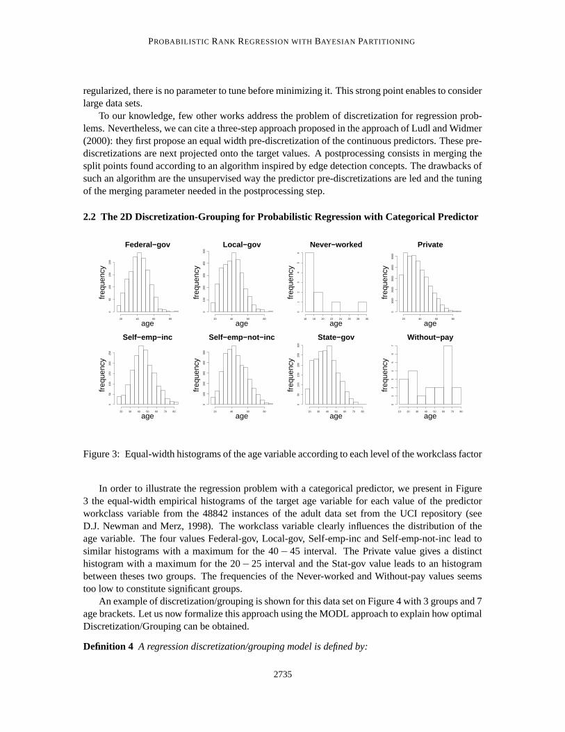
Figure 3: Equal-width histograms of the age variable according to each level of the workclass factor

In order to illustrate the regression problem with a categorical predictor, we present in Figure3 the equal-width empirical histograms of the target age variable for each value of the predictorworkclass variable from the 48842 instances of the adult data set from the UCI repository (seeD.J. Newman and Merz, 1998). The workclass variable clearly influences the distribution of theage variable. The four values Federal-gov, Local-gov, Self-emp-inc and Self-emp-not-inc lead tosimilar histograms with a maximum for the 40− 45 interval. The Private value gives a distincthistogram with a maximum for the 20− 25 interval and the Stat-gov value leads to an histogrambetween theses two groups. The frequencies of the Never-worked and Without-pay values seemstoo low to constitute significant groups.

An example of discretization/grouping is shown for this data set on Figure 4 with 3 groups and 7age brackets. Let us now formalize this approach using the MODL approach to explain how optimalDiscretization/Grouping can be obtained.

Definition 4 A regression discretization/grouping model is defined by:

2735

HUE AND BOULLE

dens

ity

17 31.5 53.5 900.00

00.

010

0.02

00.

030

Never−worked/Private

dens

ity

17 31.5 53.5 900.00

00.

010

0.02

0

Fed−gov/Loc−gov/State−gov

dens

ity

17 31.5 53.5 900.00

00.

010

0.02

0

S−e−l/S−e−n−i/Without−pay

Figure 4: Histograms of the age variable for three groups of the workclass factor

1. a number of intervals for the target variable and a number of groups for the predictor vari-able;

2. a partition of the predictor variable in a finite number of groups;

3. for each predictor group, the repartition of the instances among the target intervals specifiedby the instance counts locally to each predictor group.

Notations

N : the number of training instances

V : the number of predictor values

I : the number of predictor groups

J : the number of target intervals

ι(ν) : the group index the ν value belongs to

Ni. : the number of instances in the predictor group i

N. j : the number of instances in the target interval j

Ni j : the number of instances in the grid cell associated to predictor group i and the targetinterval j.

A regression discretization/grouping model is then entirely characterized by the parameters{

I,J,{ι(ν)}1≤i≤V ,{

Ni j}

1≤i≤I,1≤ j≤J

}

. The number of instances N. j can be deduced by adding the

Ni j for each predictor group.We adopt the following uniform hierarchical prior for the parameters of regression discretiza-

tion/grouping models:

Definition 5 The prior for the parameters of a regression discretization/grouping model is chosenhierarchically and uniformly at each level:

2736


1. the number of groups I is uniformly distributed between 1 and V ,

2. the numbers of intervals J is independent from the number of groups, and uniformly dis-tributed between 1 and N,

3. for a given number of groups I, every partition of the predictor values into I groups isequiprobable,

4. for a given predictor group, every distribution of the instances on the target intervals isequiprobable,

5. the distributions of the target intervals on each predictor group are independent from eachother,

6. for a given target interval, every distribution of the rank of the target values is equiprobable.

The definition of the regression discretization/grouping model space and its prior distribution leadsto the evaluation criterion given in Formula (3) for a discretization/grouping model M:

c(M) = log(V )+ log(N)+ logB(V, I)+I

∑i=1

log

(

Ni. + J−1J−1

)

+I

∑i=1

logNi.!

Ni,1!Ni,2! . . .Ni,J!+

J

∑j=1

logN. j!,

(3)

where B(V, I) is the number of ways to partition V values into I groups (possibly empty). For I = V ,B(V, I) corresponds to the Bell number. In general, B(V, I) can be written as a sum of Stirlingnumbers of the second kind S(V, i) (number of ways to partition a set of V values into i nonemptysubsets) (see Abramowitz and Stegun, 1970):

B(V, I) =I

∑i=1

S(V, i).

This criterion can be deduced from the grouping criterion in classification (see Boulle, 2005) andthe 2D discretization criterion in regression presented in the previous section.

3. From 2D Partitioning to Rank Predictive Cumulative Distribution Estimate

In this section we expose how we can build a univariate estimator of the rank predictive densityfrom each 2D partition and how to obtain multivariate predictors under the naive Bayes assumption.

3.1 From Values to Normalized Training Ranks and Vice-Versa

As seen in the precedent section, the MODL partitions are defined only with the ranks of the traininginstances and not with their values. Given NT numerical training values DT = (yT

1 , . . . ,yTNT

), the NT

ranked values are noted yT(1), . . . ,y

T(NT ) once the training values have been sorted.

A partition of the NT ranked instances defined by J numbers N1, . . . ,NJ such that ∑Jj=1 N j = NT

is associated to a partition of the values as follows: we define J−1 boundaries b1, . . . ,bJ−1 by b j =

2737

HUE AND BOULLE

6 6

y(1) y(NT )y(N1)

b1 =y(N1)+y(N1)+1

2 bJ−1

N1 NJ

−∞ +∞

Figure 5: Value partition from the partition frequencies: for example, the upper bound of the firstinterval containing N1 instances is the mean of the last value of this interval and of thefirst value of the second interval.

yT(β j)

+yT(β j+1)

2 where β j = ∑ jl=1 Nl and the J value partition intervals are ]−∞,b1[, [b1,b2[, . . . , [bJ−1,+∞[.

For a numerical value, its rank interval index is equal to its value interval index. This value partitionfrom the partition frequencies is illustrated in Fig 5.

As presented in the introduction, ordinal regression aims at predicting an ordinal variable whichtakes a finite number of ordered values, most of the time already known in advance. In our case, weaim at giving a finer grain prediction by considering the set of the NT possible ranks of a training dataset of size NT . In order to manipulate normalized values in [0,1], we consider the NT elementaryequal-width rank intervals of [0,1] denoted by Ten for n = 1, . . . ,NT and equal to Te1 = [0, 1

NT[,Te2 =

[ 1NT

, 2NT

[, . . . ,TeNT = [NT−1NT

,1]. These intervals are centered on the normalized ranks RDT (yT(n)) =

12NT

+ nNT

of the training instances obtained by projection on [0,1] of the rank of yT(n) among DT .

This normalization is illustrated in Fig 6.

6 6 6

y(NT )

• •• •

12NT

+ 1NT

12NT

+ 2NT

NT−1NT

0 11NT

y(1) y(2)

Figure 6: From sorted values to normalized ranks: for example, the normalized rank related to thefirst value yT

(1) is RDT (yT(1)) = 1

2NT+ 1

NT, which is the center of the first elementary interval

Te1 = [0, 1NT

[.

In practice, there may be equal values in DT . In this case, we affect the averaged rank to theconcerned instances. For a new value y unseen during training, we define its rank RDT (y) as theaverage of the normalized ranks of yT

(n1)and yT

(n2)such that yT

(n1)≤ y < yT

(n2). The integers n1 and

n2 may not be consecutive if one of them is associated with several equal values. In the rest of thepaper, we use either ranks or values depending on the context.

2738


We now detail how to build an estimate of the predictive cumulative distribution function ofthe target standardized rank from a univariate MODL 2D discretization in a first section and frommultiple univariate partitionings in a second section.

3.2 Univariate Case

We illustrate the construction of the univariate estimator from the 2D partitioning on a syntheticdata set proposed during the recent predictive uncertainty in environmental modelling competition(see Cawley et al., 2006). This data set, called synthetic, contains NT = 384 training instances andone numerical predictor. The scatter plot and the optimal MODL partition are presented in Figure 7.The optimal MODL rank intervals are denoted Pi for i = 1, . . . ,7 for predictor and Tj, j = 1, . . . ,5 forthe target. The first and the last rank intervals are of the form [0, k f /NT [ and [kl/NT , 1] respectivelyand the other intervals are of the form [k1/NT , k2/NT [. The value interval bounds x1, . . . ,x6 andy1, . . . ,y4 are obtained by projecting the frequencies partition on the value partition as described in3.1. For the predictor component x of a new instance whose rank range is Pi(x), the number of

-3

-2

-1

0

1

2

3

0 0.5 1 1.5 2 2.5 3 3.5

X

Y

x1 x2 x3 x4 x5x6

y1

y2

y3

y4

P1 P2 P3 P4 P5 P6 P7 TotalT5 1 0 0 6 5 0 0 12T4 4 68 5 2 9 0 0 88T3 38 5 26 32 24 0 0 125T2 9 0 6 33 15 21 0 84T1 0 0 0 34 4 9 28 75

Total 52 73 37 107 57 30 28 384

Figure 7: Scatter plot, 2D partitioning and numbers of the MODL grid for the synthetic data set.

examples in each grid cell give us an estimator of the probability that the target standardized rankbelongs to a given range Tj:

PModl (RDT (y) ∈ Tj | RDT (x) ∈ Pi(x)) =Ni j

Ni..

Assuming that the conditional rank density is constant over each rank interval, the probabilities ofthe elementary intervals Ten for n = 1, . . . ,NT are given by:

PModl (RDT (y) ∈ Ten | RDT (x) ∈ Pi(x)) =Ni j

Ni.N. jfor j such that Ten ⊂ Tj. (4)

We obtain an estimate of the nth NT -quantile n/NT of the conditional cumulative distribution forn = 1, . . . ,NT by summing these elementary probabilities.

The MODL estimators are plotted for each of the seven rank predictor ranges on Figure 8 for thesynthetic data set. The marks on the x−axis correspond to the normalized target ranks of the bound-aries training instances exhibited by the target partition: 75

384 ≈ 0.19, 75+84384 ≈ 0.41, 75+84+125

384 ≈ 0.74and 75+84+125+88

384 ≈ 0.97 which correspond to the projection of the value bounds y1, y2, y3 and y4

2739

HUE AND BOULLE

rg(y)0.00 0.41 0.740.

00.

40.

8

estimated F(rg(y)|x<x1)

rg(y)0.00 0.41 0.740.

00.

40.

8


rg(y)0.00 0.41 0.740.

00.

40.

8


rg(y)0.00 0.41 0.740.

00.

40.

8


rg(y)0.00 0.41 0.740.

00.

40.

8


rg(y)0.00 0.41 0.740.

00.

40.

8


rg(y)0.00 0.41 0.740.

00.

40.

8


Figure 8: MODL estimators of the conditional univariate standardized rank cumulative distributionfor the seven predictor rank ranges.

on the normalized ranks. The shape differences illustrate the seven distinct zones characterized bythe MODL optimal partition.

In the case of categorical predictors, the rank predictive cumulative distribution estimator canbe obtained in the same way by replacing the predictor intervals by predictor groups.

3.3 Multivariate Case

In the case of several predictors (K with K > 1), a first approach is to build an estimator under thenaive Bayesian assumption that the predictors are independent given the target. Let x = (x1, . . . ,xK)be the coordinates of a new instance in the predictors space and Pk

ik(x) the discretization interval(or group of values) to which belongs each component xk and Rk

DT (x) its rank. Under the naiveBayesian assumption, the elementary probability can be written :

P(

RDT (y) ∈ Ten | (R1DT (x), . . . ,RK

DT (x)) ∈ (P1i1(x), . . . ,P

KiK (x))

)

∝ P(RDT (y) ∈ Ten)K

∏k=1

P(

RkDT (x) ∈ Pk

ik(x)|RDT (y) ∈ Ten

)

= P(RDT (y) ∈ Ten)K

∏k=1

P(RDT (y) ∈ Ten|RkDT (x) ∈ Pk

ik(x))P(RkDT (x) ∈ Pk

ik(x))

P(RDT (y) ∈ Ten).

(5)

This last expression can be estimated with the instance numbers in the 2D grid cells. The first factorP(RDT (y)∈ Ten) can be estimated by the empirical probability 1/NT . Each factor of the product canbe computed from the numbers of the 2D partitioning of the target and of the kth predictor, denoted(Ik,Jk,Nk

ik.,Nkik jk) :

P(RDT (y) ∈ Ten|RkDT (x) ∈ Pk

ik(x)) =Nk

ik jk

Nkik.

Nk. jk

according to (4).

2740


P(RkDT (x) ∈ Pk

ik(x)) =Nk

ik.

NTand P(RDT (y) ∈ Ten) =

1NT

.

Each factor reduces to the fractionNk

ik jk

Nk. jk

and the elementary probabilities in Formula 5 reduce to

1NT

∏Kk=1

Nkik jk

Nk. jk

.

However, the independence hypothesis assumed in the naive Bayes predictor is usually violatedfor real data sets. In this case, estimates of the conditional probabilities are deteriorated as alreadynoticed in the work of Frank et al. (1998). For classification tasks, variable selection has beenemployed to build selective naive Bayes classifiers. This procedure reduces the strong bias of thenaive independence assumption. The objective is to search among all the subsets of variables,in order to find the best possible classifier, compliant with the naive Bayes assumption. Severalselection criteria have been tested, such as the accuracy criterion (see Langley and Sage, 1994), thearea under receiver operating characteristic (ROC) curve (see Provost et al., 1998) or the posteriorprobability of the model given the data proposed in the work of Boulle (2007). In this last case, theposterior probability is written as the sum of the prior probability of the model and of the likelihoodof the data given the model. The prior is chosen such that each specific small subset of variableshas a greater probability than each specific large subset of variables in order to favour small models.For a given subset of variables, the likelihood is computed using the naive Bayes assumption.

We propose here to build selective naive Bayes rank predictors using a MAP approach as inBoulle (2007). The extension to rank regression tasks is straightforward: the prior law remainsunchanged and, for a given subset of variables, the likelihood of the ranks of the instances arecomputed assuming the naive Bayes assumption according to (5).

To summarize this section, we have exposed how the 2D partitionings give us estimators ofquantiles of the univariate or multivariate rank cdf. The choice of the estimated quantiles are givenby the univariate partitionings. Let us see, in the next section, on which criterion such probabilisticrank models can be evaluated.

4. Performance Evaluation for Probabilistic Rank Regression

For deterministic predictive models, performance evaluation consists in evaluating the distance be-tween the predicted class or value and the true class or value. Depending on the metric used, severalperformance measures can be used such as the mean absolute error or the mean squared error.

For probabilistic predictive models, performance evaluation consists in comparing the true valueor class with an estimate of its conditional cumulative distribution function (cdf) or an estimate ofits conditional probability density function (pdf). It is measured through a score function which canbe negatively oriented (large values imply poor performance) or positively oriented (large valuesimply high performance). A score function is said to be proper if its expectation is maximized (orminimized) for the true predictive distribution. It is said strictly proper if this optimum is unique.

Among the strictly proper scoring functions, the two more commonly used are the logarithmicand the quadratic scores (see Gneiting and Raftery, 2004). They take different forms depending onthe learning task. In the sequel, we first describe the quadratic and the logarithmic scores and theiruse in classification and regression. We then present an interesting way to build the logarithmicscore function from ranks rather than from values.

2741

HUE AND BOULLE

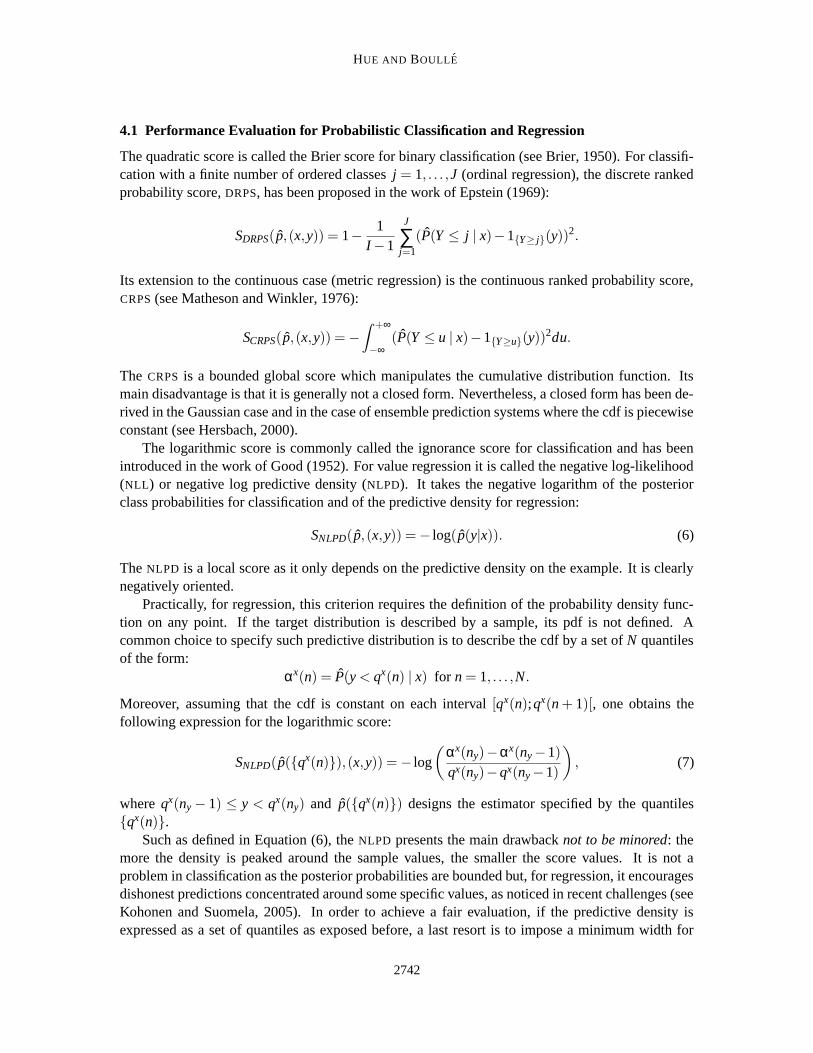
4.1 Performance Evaluation for Probabilistic Classification and Regression

The quadratic score is called the Brier score for binary classification (see Brier, 1950). For classifi-cation with a finite number of ordered classes j = 1, . . . ,J (ordinal regression), the discrete rankedprobability score, DRPS, has been proposed in the work of Epstein (1969):

SDRPS(p,(x,y)) = 1−1

I−1

J

∑j=1

(P(Y ≤ j | x)−1{Y≥ j}(y))2.

Its extension to the continuous case (metric regression) is the continuous ranked probability score,CRPS (see Matheson and Winkler, 1976):

SCRPS(p,(x,y)) =−Z +∞

−∞(P(Y ≤ u | x)−1{Y≥u}(y))

2du.

The CRPS is a bounded global score which manipulates the cumulative distribution function. Itsmain disadvantage is that it is generally not a closed form. Nevertheless, a closed form has been de-rived in the Gaussian case and in the case of ensemble prediction systems where the cdf is piecewiseconstant (see Hersbach, 2000).

The logarithmic score is commonly called the ignorance score for classification and has beenintroduced in the work of Good (1952). For value regression it is called the negative log-likelihood(NLL) or negative log predictive density (NLPD). It takes the negative logarithm of the posteriorclass probabilities for classification and of the predictive density for regression:

SNLPD(p,(x,y)) =− log(p(y|x)). (6)

The NLPD is a local score as it only depends on the predictive density on the example. It is clearlynegatively oriented.

Practically, for regression, this criterion requires the definition of the probability density func-tion on any point. If the target distribution is described by a sample, its pdf is not defined. Acommon choice to specify such predictive distribution is to describe the cdf by a set of N quantilesof the form:

αx(n) = P(y < qx(n) | x) for n = 1, . . . ,N.

Moreover, assuming that the cdf is constant on each interval [qx(n);qx(n + 1)[, one obtains thefollowing expression for the logarithmic score:

SNLPD(p({qx(n)}),(x,y)) =− log

(

αx(ny)−αx(ny−1)

qx(ny)−qx(ny−1)

)

, (7)

where qx(ny − 1) ≤ y < qx(ny) and p({qx(n)}) designs the estimator specified by the quantiles{qx(n)}.

Such as defined in Equation (6), the NLPD presents the main drawback not to be minored: themore the density is peaked around the sample values, the smaller the score values. It is not aproblem in classification as the posterior probabilities are bounded but, for regression, it encouragesdishonest predictions concentrated around some specific values, as noticed in recent challenges (seeKohonen and Suomela, 2005). In order to achieve a fair evaluation, if the predictive density isexpressed as a set of quantiles as exposed before, a last resort is to impose a minimum width for

2742


scoring rule quadratic score logarithmic scorebinary classification Brier score Ignorance scoreordinal regression DRPSvalue regression CRPS NLPD

Table 1: Quadratic and logarithmic scores for performance evaluation of probabilistic predictivemodels

the intervals [qx(n−1);qx(n)[. Anyway, such a score function contributes to confusing performanceprediction since arbitrary small values can be obtained fortunately.

The two scores mentioned above are presented in Table 1.Let now study what happens if we compute the logarithmic score for the rank predictive density

rather than for the value predictive density.

4.2 A Robust Logarithmic Score Defined on the Rank Predictive Density

Given a training data set set DT = (xTn ,yT

n )n=1,...,NT , we assume that we have at our disposal arank probabilistic estimator specified for any given x by the NT estimated quantiles αx(n) forn = 1, . . . ,NT of the standardized rank cumulative distribution function:

αx(n) = P(RDT (y) <n

NT|x) for n = 1, . . . ,NT .

We can immediately see that this assumption is not restrictive: knowing the values associated to theranks, each value estimator gives us an estimator of the cdf on the NT target normalized ranks of thetraining data set. If we denote by y(n) the nth target value of DT , we have :


NT|x) = P(y <

y(n) + y(n+1)

2|x). (8)

By appropriate integration of the cdf, each value estimator specified by N given quantiles gives usthe NT quantiles estimates defined in (8).

Let us come back to the evaluation of such a rank probabilistic estimator with the logarith-mic score function. It consists in comparing it with the standardized insertion rank RDT (y) of thetrue value y among the training data set DT . We propose to estimate the predictive density on theinsertion rank by the ratio:

p(RDT (y)|x)≈P(RDT (y) ∈ Teny | x)

1/NT,

where Teny is the elementary interval to which the insertion rank RDT (y) belongs.This approximation enables us to define the Negative Log Rank Predictive Density as follows:

Definition 6 Let a training data set set DT = (xTn ,yT

n )n=1,...,NT and αx(n) for n = 1, . . . ,NT someestimates of the NT quantiles of the standardized rank cumulative distribution function:


NT|x) for n = 1, . . . ,NT .

2743

HUE AND BOULLE

Rank predictive distribution specification: Let DT = (xTn ,yT

n )n=1,...,NT be a training dataset with Y a numerical target and X = (X 1, . . . ,XK) K numerical or categorical predictors.For any given x, the rank predictive distribution is specified by the NT quantiles of therank cdf:


NT| x) for n = 1, . . . ,NT .

Rank predictive distribution evaluation: Let DV = (xVn ,yV

n )n=1,...,NV be a validation dataset. Compute the logarithmic score of the rank predictive distribution on data set DV as

NLRPD =−1

NV

NV

∑n=1

logαxV

n (ny)−αxVn (ny−1)

1/NT,

where RDT (yv), the standardized insertion rank of the true value yVn among the training

data set DT , is included in the elementary interval Teny .

Table 2: Summary of the proposed approach for probabilistic standardized rank regression and itsevaluation.

The score function for the negative log rank predictive density is then defined by:

SNLRPD(P(NT ),(x,y)) =− logP(RDT (y) ∈ Teny | x)

1/NT

=− log(αx(ny)−αx(ny−1))− log(NT ),

(9)

where P(NT ) is the rank predictive density estimator specified by the quantiles { nNT}. We now

present two interesting properties of the NLRPD.

Theorem 7 In absence of predictive information the NLRPD is equal to zero.

Without any predictive information, the probability that the insertion rank of a new instance belongsto a given interval is simply equal to 1/NT . By construction, we have then for the uniform predictorPuni f (NT ):

SNLRPD(Puni f (NT ),(x,y)) =− log1 = 0.

�

Moreover, unlike the NLPD score, this score function on ranks has the great advantage to beminored as it is precised in the following property:

Theorem 8 Given a training data set set DT of size NT , the NLRPD score function is minored by− log(NT ).

This bound is directly obtained by considering that the difference αx(ny)−αx(ny− 1) belongs to]0;1].�

By construction, the proposed NLRPD score is then bounded. However, it depends on thetraining data set through its size. We will see in next section its relative insensitivity to this size.

2744


Let us now examine the link between the score function on ranks and the score function onvalues. Using the expression (7) with the NT −1 quantiles b1 =

y(1)+y(2)

2 , b2 =y(2)+y(3)

2 , . . ., bNT−1 =y(NT−1)+y(NT )

2 , we obtain the relation :

SNLRPD(P(NT ),(x,y)) = SNLPD(p({bny}),(x,y))− log(NT )− log(bny−bny−1).

As precised at the beginning of the section, the NLRPD score function can be used by convertingany value predictive density estimator to rank predictive density estimator specified or using theabove relation between NLRPD and NLPD score functions.

The framework of our approach is summarized in Table 2.

5. Experimental Evaluation

We first present experiments about the criteria proposed in the precedent section. Then, we focuson the quality of the 2D-partitioning with experiments on synthetic data. We finish by experimentswith the univariate and multivariate predictors presented on five real data sets.

5.1 Experiments on the NLRPD

We focus here on the properties of the proposed criterion, the NLRPD. We consider the data gener-ated according to the following heteroscedastic model (used for the synthetic data set of the predic-tive uncertainty in environmental modeling competition):

{

xn ∼U[0π]

yn ∼N(

sin(

5x2

)

sin(

3x2

)

, 1100 + 1

4

(

1− sin(

5x2

))2)

This data set has been used in Section 3 to describe the building of the rank conditional densities.Knowing the true cdf of the synthetic data set, we can compute the true NLRPD by using the trueprobabilities instead of their estimates in (9).

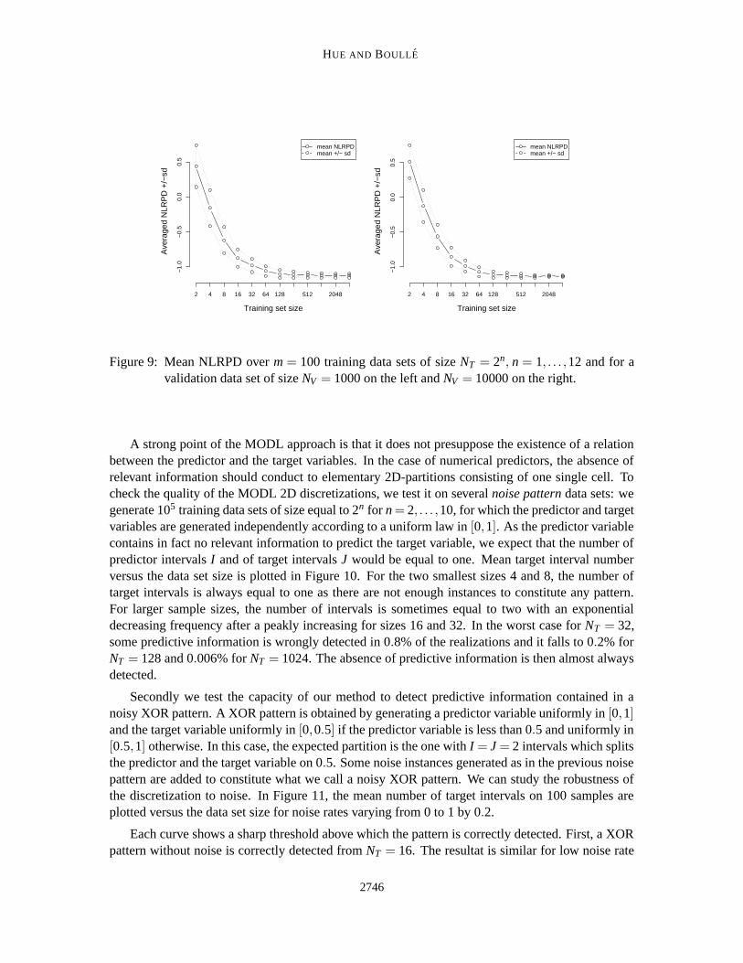
The contentious aspect of the NLRPD is that it depends on the training data set size. Theobjective of this experiment is then to study the sensitivity of the NLRPD with respect to the trainingsize in a first time and to the validation data set size in a second time. For that, we have generatedm = 100 training data sets of size NT = 2n for n = 1, . . . ,12. The true NLRPD has been computedgiven each of the m ∗ 12 training quantile vectors for a test data set of size NV = 1000 and anotherone of size NV = 10000. The mean NLRPD over the m training data sets is plotted versus thetraining data set size NT on left of Figure 9 for NV = 1000 and on right for NV = 10000.

First, this plot shows a threshold around a training data set size of NT = 100 instances. Belowthis threshold, the true NLRPD decreases when the training set size increases. Above this threshold,the optimal NLRPD seems insensitive to the training set size. Secondly, we can notice that bothcurves for NV = 1000 and NV = 10000 are very similar. This allows us to think the NLRPD is notvery sensitive to the test data set size. To confirm this fact, we have fixed a training data set of size384 and we have computed the true NLRPD for m = 100 test data sets of size NV = 1024. Thestandard-deviation obtained is around 3%. Our criterion looks robust with respect to the trainingand validation data set size.

5.2 Experiments on the 2D-Partitioning

In this section, we focus on the quality of the 2D-partitioning with three experiments.

2745

HUE AND BOULLE

Training set size

Ave

rage

d N

LRP

D +

/−sd

2 4 8 16 32 64 128 512 2048

−1.

0−

0.5

0.0

0.5

●

●

mean NLRPDmean +/− sd

Training set size

Ave

rage

d N

LRP

D +

/−sd

2 4 8 16 32 64 128 512 2048

−1.

0−

0.5

0.0

0.5

●

●

mean NLRPDmean +/− sd

Figure 9: Mean NLRPD over m = 100 training data sets of size NT = 2n, n = 1, . . . ,12 and for avalidation data set of size NV = 1000 on the left and NV = 10000 on the right.

A strong point of the MODL approach is that it does not presuppose the existence of a relationbetween the predictor and the target variables. In the case of numerical predictors, the absence ofrelevant information should conduct to elementary 2D-partitions consisting of one single cell. Tocheck the quality of the MODL 2D discretizations, we test it on several noise pattern data sets: wegenerate 105 training data sets of size equal to 2n for n = 2, . . . ,10, for which the predictor and targetvariables are generated independently according to a uniform law in [0,1]. As the predictor variablecontains in fact no relevant information to predict the target variable, we expect that the number ofpredictor intervals I and of target intervals J would be equal to one. Mean target interval numberversus the data set size is plotted in Figure 10. For the two smallest sizes 4 and 8, the number oftarget intervals is always equal to one as there are not enough instances to constitute any pattern.For larger sample sizes, the number of intervals is sometimes equal to two with an exponentialdecreasing frequency after a peakly increasing for sizes 16 and 32. In the worst case for NT = 32,some predictive information is wrongly detected in 0.8% of the realizations and it falls to 0.2% forNT = 128 and 0.006% for NT = 1024. The absence of predictive information is then almost alwaysdetected.

Secondly we test the capacity of our method to detect predictive information contained in anoisy XOR pattern. A XOR pattern is obtained by generating a predictor variable uniformly in [0,1]and the target variable uniformly in [0,0.5] if the predictor variable is less than 0.5 and uniformly in[0.5,1] otherwise. In this case, the expected partition is the one with I = J = 2 intervals which splitsthe predictor and the target variable on 0.5. Some noise instances generated as in the previous noisepattern are added to constitute what we call a noisy XOR pattern. We can study the robustness ofthe discretization to noise. In Figure 11, the mean number of target intervals on 100 samples areplotted versus the data set size for noise rates varying from 0 to 1 by 0.2.

Each curve shows a sharp threshold above which the pattern is correctly detected. First, a XORpattern without noise is correctly detected from NT = 16. The resultat is similar for low noise rate

2746


5 10 20 50 100 200 500 1000

1.00

01.

002

1.00

41.

006

1.00

8

Dataset size

Ave

rage

d in

terv

al n

umbe

r

IJ

Figure 10: Mean target and predictor interval numbers for 100000 noise pattern data sets of size 4to 1024

5 10 50 100 500 5000

1.0

1.2

1.4

1.6

1.8

2.0

Sample size

Ave

rage

d ta

rget

inte

rval

num

ber

00.20.40.60.81

Figure 11: Mean target interval number for 100 noisy XOR pattern data sets of size 4 to 5096 fornoise rate = 0,0.2,0.4,0.6,0.8,1.

equal to 0.2. This threshold increases with the noise rate and reachs respectively 128, 256 and 1024for a rate equal to 0.4, 0.6 and 0.8. Our discretization is then robust to noise rate.

2747

HUE AND BOULLE

−1.0 −0.5 0.0 0.5 1.0

−1.

0−

0.5

0.0

0.5

1.0

x

y

Figure 12: Optimal MODL 2D-partition for data on a noisy circle.

Thirdly, we test the capacity of our method to detect multimodality. For that we generate 300instances on a noisy circle as showed in Figure 12. The density of y conditionally to x is bimodal formost values of x. As there is no assumption in the MODL approach about the form of the conditionaldistribution, the 2D-partitioning can produce multimodal conditional densities. For the noisy circledata set, the optimal MODL 2D-partition plotted in Figure 12 clearly shows the two modes of thelaw.

5.3 Experiments on Real Data Sets

In this section, we test the estimators proposed in Section 3 on real data . We have chosen thefollowing five regression data sets, detailed in Table 3:

• SO2, precip and temp, available from the predictive uncertainty competition website(http://theoval.cmp.uea.ac.uk/competition/).

• Adult and housing (Boston), available from the UCI machine learning repository(http://www.ics.uci.edu/ mlearn/MLSummary.html);

Data Set SO2 Precip Temp Adult HousingNumerical predictors 27 106 106 6 13Categorical predictors 0 0 0 7 0Number of patterns 22956 10546 10675 48842 506

Table 3: Summary of the dimensions of five data sets chosen to evaluate the probabilistic rankpredictive density estimators.

For each data set, we have performed a five-fold cross validation for the three following estimators:

2748


SO2 Level I J Precip Level I J Temp Level I JV7 0.01467 9 7 V3 0.01986 5 6 V102 0.1234 13 14V25 0.00993 7 6 V35 0.01858 5 6 V104 0.1095 12 13V27 0.009658 7 7 V4 0.01823 5 6 V101 0.1069 13 12V2 0.009483 6 28 V81 0.01729 4 6 V103 0.1039 12 13V26 0.008302 6 7 V69 0.01716 4 7 V100 0.06891 9 12V1 0.003991 5 127 V36 0.01674 4 7 V98 0.06288 9 10V11 0.001366 5 5 V82 0.01653 4 6 V106 0.05691 8 8V8 0.0009511 3 4 V70 0.01633 4 6 V99 0.05614 8 9V12 0.0008027 4 3 V57 0.01632 4 6 V97 0.05566 9 10V18 0.0007759 3 4 V45 0.01629 4 6 V6 0.03347 7 7

Adult Level I J Housing Level I Jmarital-status 0.0244 11 6 LSTAT 0.0945 5 5relationship 0.01936 12 5 RM 0.06378 5 5hours-per-week 0.009682 10 6 NOX 0.04466 5 5education 0.009164 10 9 INDUS 0.04350 3 5education-num 0.009016 9 9 PTRATIO 0.03779 5 4class 0.006555 10 2 CRIM 0.03451 4 5occupation 0.003556 7 7 TAX 0.03352 4 5workclass 0.002672 6 5 AGE 0.03208 4 3capital-gain 0.002257 4 18 DIS 0.02929 5 3sex 0.0007349 3 2 RAD 0.01977 3 2

Table 4: Compression gains (levels) and size (I,J) of the 2D partitions for the ten most informativevariables of the 1-fold of the five data sets.

• the univariate estimator built with the most MODL informative variable;

• the multivariate estimator built under the naive Bayes assumption with all the predictor vari-ables (NB);

• the multivariate estimator built under the naive Bayes assumption with the best selected subsetof predictor variables (SNB).

For each fold, the estimators are built from the optimal MODL 2D-discretizations for each couple(predictor,target). The compression gain (or level) defined in (2) enables us to rank the predic-tors. For illustration, Table 4 presents the level and the size (I,J) of the 2D partitions for the bestpredictors, for the first training set of each data set.

Each estimator is evaluated with the NLRPD criteria proposed in the previous section. Table 5presents the mean and standard-deviation of the NLRPD for each data set and each estimator.

First, we can see the poor performance of the naive Bayes estimator which exploits all the uni-variate predictors: for all data sets except for the adult data set, the NLRPD for the NB estimatoris positive that is to say it performs not as good as the predictor built without any predictive infor-mation. This phenomenon is due to the violation of the naive Bayes assumption. For example, in

2749

HUE AND BOULLE

Univariate SNB NBSO2 -0.136 +/- 0.003 -0.162 +/- 0.0076 0.24 +/- 0.036Precip -0.165 +/- 0.005 -0.220 +/- 0.023 9.0 +/- 1.36Temp -1.018 +/- 0.012 -1.046 +/- 0.0173 5.46 +/- 0.99Adult -0.237+/- 0.0048 -0.378+/- 0.03 -0.287 +/- 0.029Housing -0.393+/- 0.128 -0.26 +/- 0.26 0.849+/- 0.49

Table 5: Mean and standard-deviation of the NLRPD for the 3 predictors and the five real data sets.

the case of the temp data set, Figure 13 presents the scatter plot of the two most informative vari-ables. The very high linear correlation clearly deteriorates the naive Bayes predictor based on thesevariables.

−4 −3 −2 −1 0 1 2 3

−3

−2

−1

01

23

V102

V10

4

Figure 13: Scatter plot of the two most informative variables for the temp data set.

The second point from these results is the relative good performance of the univariate predictor.For the SO2, precip and temp data sets, it performs nearly as well as the SNB, which selects aroundfive predictors, even if the NLRPD mean for the SNB is significantly lower than for the univariatepredictor according to a Student’s t-test. These three data sets seem a bit specific in the sense thatthe most informative variable contains a lot of the predictive information. The good 2D partitioningquality enables to build a very performant univariate predictor. For the adult data set, the SNB,which selects around 9 predictors, performs better than the NB which performs better than theUnivariate predictor. The predictive information is shared by several variables and the selectionprocedure enables to eliminate redundant predictors like education and education-num, or marital-status and relationship. For the housing data set, the univariate predictor performs as well as theSNB which selects around five predictors. The variance of the results is important which certainlyexplains that the equality hypothesis of the means is not rejected according to a Student t-test. It

2750


NLPD on test set SO2 Precip TempOrganizer’s method 4.25 (1st) -0.509 (1st) 0.053 (2nd)Best submitted method 4.37 (3th) -0.279 (3th) 0.034 (1st)MODL SNB 4.31 (2nd) -0.437 (2nd) 0.259 (8th)MODL Univariate 4.33 (2nd) -0.361 (2nd) 0.284 (8th)Reference method 4.5 (4th) -0.177 (4th) 1.30 (9th)

Table 6: NLPD values for each test data set for the univariate estimator using the best MODLpredictor (MODL univariate), the selective naive Bayes predictor (MODL SNB), the bestmethod in competition, the organizer’s submission and the reference method. The rankingof each method is between brackets after each NLPD value.

may seem surprising that the univariate sometimes performs better than the SNB. The reason maybe that the selection procedure in the SNB assumes that the univariate predictors are perfect andfocuses on the choice of the number of variables. In other words, the uncertainty of the univariatepredictive model is not taken into account at this stage. It also suggests that the SNB predictorcould be improved. Contrary to the classification case, the target partition is different for eachpredictor considered. This aspect could be taken into account in the selection of the predictors.Model averaging could also improve our multivariate predictors.

The objective of our last experiment is to compare our approach with other regression methods.To our knowledge, there is no alternative rank regression method available in the literature. Wetherefore compare it to value predictive density estimators. Such estimators being still an activesubject of research, we decide to compare our approach to the methods proposed very recentlyin the predictive uncertainty in environmental modelling competition organized in 2006 by GavinCawley. Since these methods are hard to re-implement and tune, we project our rank estimator to avalue estimator and we compare them with the NLPD criteria. Knowing the values associated to theranks, each rank estimator gives us an estimator of the cdf on the NT target values of the trainingdata set using (8). To compute the predictive pdf on any point from the conditional quantiles, weadopt the same assumptions as those used in the challenge, that is that the pdf is assumed uniformbetween two successive values and that the distribution tails are exponential.1

As our approach is implicitly regularized and needs no tuning parameter, we use the training andvalidation data sets to compute the optimal 2D partitionings. Given the poor performance of the NBin the previous experiments, we only train the univariate and the SNB predictors. Table 6 indicatesthe NLPD on the test data set for these two MODL estimators, the best method in competitionand the reference method which computes the empirical estimator of the marginal law p(y). Forthe three data sets, the MODL estimators are better than the reference method, that is far frombeing the case for all submitted methods. Secondly, we observe good performance for the MODLestimators, in particular for the SO2 and Precip data sets where the SNB estimator is at the frontafter the organizer’s method. The good performance of the univariate predictor demonstrates the2D partitioning quality despite the use of the ranks and not of the values for this step. Moreover, theSNB estimator is always better than the univariate estimator. This proves the presence of additionalinformation and the interest of the selection procedure.

1. For that we affect an ε = 1/2N probability mass at each tail.

2751

HUE AND BOULLE

6. Conclusion

We have first proposed a non parametric Bayesian approach for the estimation of the conditionaldistribution of the normalized rank of a numerical target. Our approach is based on an optimal2D partitioning of each couple (target, predictor). These partitionings are used to build univariateestimators and multivariate ones under the naive Bayesian assumption of predictors conditionalindependence, with and without variable selection.

Our approach is applicable for all regression problems with categorical or numerical predictors.It is particularly interesting for those with a high number of predictors as it automatically detectsthe variables which contain predictive information. As the criteria selection is regularized by thepresence of a prior and a posterior term, it does not suffer from overfitting.

Secondly we have proposed a new criterion to evaluate a probabilistic estimator of the rankpredictive density. It uses the logarithmic score and presents the main advantage to be minoredcontrary to the logarithmic score computed for probabilistic estimators of the target value. As avalue estimator can be projected on a rank estimator, this criterion provides a reliable evaluationcriterion for all probabilistic regression estimators on values or on ranks.

Experiments on synthetic data sets show the validity of the proposed evaluation criterion andthe quality of the 2D partitioning. Experiments on real data sets show the failure of the naive Bayesbut the potential of the selective naive Bayes estimator. A comparison with methods proposed ina recent challenge dedicated to probabilistic metric regression methods evaluates the competitivityof our approach after the projection of our rank estimators on the value range. The very goodperformance of our best univariate and selective naive Bayes estimators encourages us to work inthe future to improve the SNB approach and to evaluate the potential benefit of model averaging.

Acknowledgments

We are grateful to the editor and the anonymous reviewers for their useful comments.

References

M. Abramowitz and I. Stegun. Handbook of Mathematical Functions. Dover Publications Inc.,New York, 1970.

M. Boulle. A Bayes optimal approach for partitioning the values of categorical attributes. Journalof Machine Learning Research, 2005.

M. Boulle. MODL: A Bayes optimal discretization method for continuous attributes. MachineLearning, 65(1):131–165, 2006.

M. Boulle. Compression-based averaging of selective naive Bayes classifiers. Journal of MachineLearning Research, To appear, 2007.

M. Boulle and C. Hue. Optimal Bayesian 2d-discretization for variable ranking in regression. InNinth International Conference on Discovery Science (DS 2006), 2006.

G. W. Brier. Verification of forecasts expressed in terms of probability. Monthly Weather Review,78(1):1–3, 1950.

2752


G.C. Cawley, M.R. Haylock, and S.R. Dorling. Predictive uncertainty in environmental modelling.In 2006 International Joint Conference on Neural Networks, pages 11096–11103, 2006.

P. Chaudhuri and W.-Y. Loh. Nonparametric estimation of conditional quantiles using quantileregression trees. Bernouilli, 8, 2002.

P. Chaudhuri, M.-C. Huang, W.-Y. Loh, and R. Yao. Piecewise-polynomial regression trees. Statis-tica Sinica, 4, 1994.

W. Chu and Z. Ghahramani. Gaussian processes for ordinal regression. Journal of Machine Learn-ing Research, 6:1019–1041, 2005.

W. Chu and S. Keerthi. New approaches to support vector ordinal regression. In ICML ’05: Pro-ceedings of the 22nd international conference on Machine Learning, 2005.

K. Crammer and Y. Singer. Pranking with ranking. In Proceedings of the Fourteenth AnnualConference on Neural Information Processing Systems (NIPS), 2001.

C.L. Blake D.J. Newman, S. Hettich and C.J. Merz. UCI repository of machine learning databases,1998. URL http://www.ics.uci.edu/∼mlearn/MLRepository.html.

E. S. Epstein. A scoring system for probability forecasts of ranked categories. Journal of AppliedMeteorology, 8:985–987, December 1969.

J. Fan, Q. Yao, and H. Tong. Estimation of conditional densities and sensitivity measures in nonlin-ear dynamical systems. Biometrika, 83:189–196, 1996.

R.A. Fisher. The use of multiple measurements in taxonomic problems. Annual Eugenics, 7, 1936.

E. Frank, L. Trigg, G. Holmes, and I. Witten. Naive Bayes for regression, 1998. URLciteseer.ist.psu.edu/article/frank98naive.html. Working Paper 98/15. Hamilton,NZ: Waikato University, Department of Computer Science.

T. Gneiting and A. Raftery. Strictly proper scoring rules, prediction and estimation. Technicalreport, Department of Statistics, University of Washington, 2004.

I. Good. Rational decisions. Journal of the Royal Statistical Society, 14(1):107–114, 1952.

R. Herbrich, T. Graepel, and K. Obermayer. Large margin rank boundaries for ordinal regression,chapter 7, pages 115–132. 2000.

H. Hersbach. Decomposition of the Continuous Ranked Probability Score for ensemble predictionsystems. Weather and Forecasting, 15(5):559–570, 2000.

T. P. Hettmansperger and J. W. McKean. Robust Nonparametric Statistical Methods. Arnold,London, 1998.

R. Koenker. Quantile Regression. Econometric Society Monograph Series. Cambridge UniversityPress, 2005.

2753

HUE AND BOULLE

J. Kohonen and J. Suomela. Lessons learned in the challenge: making predictions and scoringthem. In Revised Selected Papers of the 1st PASCAL Machine Learning Challenges Workshop(MLCW, Southampton, UK, April 2005), Lecture Notes in Artificial Intelligence 3944, pages 95–116, 2005.

P. Langley and S. Sage. Induction of selective Bayesian classifiers. In In Proceedings ofthe Tenth Conference on Uncertainty in Artificial Intelligence, pages 399–406, 1994. URLciteseer.ist.psu.edu/langley94induction.html.

M.-C. Ludl and G. Widmer. Relative unsupervised discretization for regression problems. InEleventh European Conference on Machine Learning (ECML-2000), pages 246–254, 2000.

J. Matheson and R. Winkler. Scoring rules for continuous probability distributions. ManagementSci., 22:1087–1096, 1976.

N. Meinshausen. Quantile regression forests. Journal of Machine Learning Research, 7:983–999,2006.

F. Provost, T. Fawcett, and R. Kohavi. The case against accuracy estimation for comparing inductionalgorithms. In In Proc. Fifteenth Intl. Conf. Machine Learning, pages 445–453, 1998. URLciteseer.ist.psu.edu/provost97case.html.

C.E. Shannon. A mathematical theory of communication. Bell Systems Technical Journal, 1948.

A. Shashua and A. Levin. Ranking with large margin principles : two approaches. In Proceedingsof the Fiveteenth Annual Conference on Neural Information Processing Systems (NIPS), 2002.

I. Takeuchi, Q.V. Le, T.D. Sears, and Smola A.J. Nonparametric quantile estimation. Journal ofMachine Learning Research, 7:1231–1264, 2006.

H White. Nonparametric estimation of conditional quantiles using neural networks. In Proceedingsof the 1991 Interface Conference, 1991.

2754

a new probabilistic approach in rank regression with optimal

Documents