a new model to predict the energy generated by a photovoltaic system connected to the grid in low...

Available online at www.sciencedirect.com

www.elsevier.com/locate/solener

ScienceDirect

Solar Energy 107 (2014) 423–442

A new model to predict the energy generated by a photovoltaicsystem connected to the grid in low latitude countries

Luis Fernando Mulcue-Nieto a,b,⇑, Llanos Mora-Lopez b,c

a GIDTA Group, Research Group in Environmental and Technological Developments, Universidad Catolica de Manizales, Carrera 23 No. 60 – 63,

Manizales, Colombiab Universidad Internacional de Andalucıa, Calle Severo Ochoa 16, 29590 Malaga, Spain

c Department of Computer Languages and Sciences, ETSI Informatica, Universidad de Malaga, Campus de Teatinos, 29071 Malaga, Spain

Received 24 February 2014; received in revised form 21 April 2014; accepted 22 April 2014

Communicated by: Associate Editor Nicola Romeo

Abstract

The use of photovoltaic solar energy is a growing reality worldwide and its main objective is to meet electricity demand in a sustain-able manner. The so-called Grid-Connected Photovoltaic Power Systems (GCPS) prevail in urban zones, together with Building-inte-grated Photovoltaics (BIPV); whose performance and energy efficiency depends on different factors. The main aspects include thoserelated to the solar radiation available in the geographical location of the facility, the climate, the orientation and tilt of the used surfaces,the appropriate design of the system and the quality of the components. Therefore, several methods have been proposed to try to predictthe influence of the aforementioned variables on the amount of electricity produced. However, the majority are very tedious to implementor do not take the specific characteristics of the system into account.

This paper proposes a simple and reliable expression, which can be used in low latitude countries. The case study is likewise performedfor Colombia, with a comparative analysis for different cities of the angular losses and due to dirt, the losses due to temperature, the DC–AC conversion losses and the Performance Ratio of the system (PR).� 2014 Elsevier Ltd. All rights reserved.

Keywords: Building-integrated Photovoltaics (BIPV); Performance Ratio (PR); Energy produced by a photovoltaic system; Performance of a photov-oltaic system

1. Introduction

Photovoltaic solar energy is an excellent option to meetthe energy demands of the world population, by means ofgenerating electricity in a distributed manner (Pearce,

http://dx.doi.org/10.1016/j.solener.2014.04.030

0038-092X/� 2014 Elsevier Ltd. All rights reserved.

⇑ Corresponding author at: GIDTA Group, Research Group in Envi-ronmental and Technological Developments, Universidad Catolica deManizales, Carrera 23 No. 60 – 63, Manizales, Colombia. Tel.: +5768782900x3300; fax: +57 68782937.

E-mail addresses: [email protected] (L.F. Mulcue-Nieto),[email protected] (L. Mora-Lopez).

2002). Thousands of electricity generators have thereforebeen installed using this process around the world. Theso-called Grid-Connected Photovoltaic Power Systems(GCPS) prevail in urban zones and they meet the energyneeds of the building or housing unit, while the surpluselectricity produced is injected into the grid.

On the other hand, installing photovoltaic panels on thesurfaces of the buildings has become necessary due to thespatial and economic restrictions. This has led to a highlyimportant and developed sector, Building-integratedPhotovoltaics (BIPV), where different construction elements


mailto:[email protected]

mailto:[email protected]


http://crossmark.crossref.org/dialog/?doi=10.1016/j.solener.2014.04.030&domain=pdf

424 L.F. Mulcue-Nieto, L. Mora-Lopez / Solar Energy 107 (2014) 423–442

such as roofs, frontages or windows are replaced by photo-voltaic modules.

One of the main goals in the field of BIPV is to achieveoptimum aesthetic, economic and technical solutions, thusmaking sure that all the new constructions will be “ZeroEnergy Buildings” (ZEB) (Kanters and Horvat, 2012). Inorder to achieve this, it is vital to forecast the amount ofelectricity produced by the facility, so the net energy bal-ance can be calculated. This calculation must be carriedout in one of the design stages of the system.

In 1998, the International Electrotechnical Commission

(IEC) published the IEC 61724 International Standard.This standard describes the recommendation for analysingthe electrical performance of the photovoltaic systems. Oneof the characteristic parameters is the annual energy pro-duced, which can be calculated using the following equa-tion for Grid-Connected Photovoltaic Power Systems(The International Electrotechnical Commission (IEC),1998):

EPV ¼Gaðb; aÞ � P peak � PR

GSTCð1Þ

where Ga(b,a) is the annual solar radiation on the generatorsurface, Ppeak is the installed photovoltaic peak power, PRthe annual yield of the facility known as the “PerformanceRatio” and GST the solar irradiance under standard mea-surement conditions, equal to 1 kW/m2.

The Ga(b,a) value can be easily obtained by means ofgraphs of the so-called Irradiation Factor (FI) (Thomas,2012; Roberts and Guariento, 2009). Therefore, the prob-lem of calculating the electricity produced is mainlyreduced to determining the PR value. Yet this task is noteasy, as the performance depends on several factors suchas the solar radiation available in the geographical locationof the facility, the climate, the orientation and tilt of theused surfaces, the appropriate design of the system andthe quality of the components, among others.

In order to solve the above problem, different methodshave been put forward to predict the influence of differentvariables on the amount of electricity generated. Some ofthem are analytical, for example, those used byOsterwald (1986), Araujo et al. (1982) or Green (1998);which allow the temperature losses to be calculated. Otherprocedures have likewise been proposed that include morevariables, based on artificial neuronal networks(Almonacid et al., 2009; Rodrigo et al., 2012). However,the majority of them are very tedious to implement, whileothers do not take into account the specific characteristicsof the system.

Another way that has been proposed to solve the prob-lem is to use a standard performance of PR = 0.75 for anyphotovoltaic system (Markvart and Castaner, 2003), whichis not appropriate as the specific variables of the place mustbe taken into account. For example, studies of PR in 8countries have been reported, obtaining values between0.42 and 0.81 (Mondol et al., 2006). This is coherent, asthe performance of the photovoltaic modules depends on

the ambient temperature of the place. Latitude likewiseplays an important role, as its effect on solar irradiationmeans that the power supplied to the entrance of the inver-ter may be very low within certain time periods, thus reduc-ing the DC–AC conversion efficiency.

Another important factor that prevents a generalisedPR being used for BIPV applications are the energy lossescaused by the tilt and orientation of the generator plane.Their origin lies in the fact that sun light is reflected morewhen the incidence angle is small with respect to the sur-face. The losses due to dust and dirt also depend on thisvariable. Thus, the PR is expected to vary for a singlebuilding, due to the large amount of surfaces available tobe used on roofs and frontages.

According to what has been discussed, the large amountof factors present makes it very difficult to forecast theperformance of the photovoltaic facility. It is therefore nec-essary to implement a simple method that can be used byarchitects and engineers. This is very important as manycountries need to expand photovoltaic solar energy. InColombia, for example, non-grid connected zones, thatis, places that are not connected to electricity by meansof the Sistema de Interconexion Nacional [Colombianpower grid] account for nearly 52% of national territory(Senado de la Republica de Colombia, 2003). Further-more, it is recommended to implement BIPV within thecities in order to obtain economic and environmentalbenefits.

This paper proposes a simple and reliable expression,which can be used in low latitude countries. The case studyis likewise performed for Colombia, with a comparativeanalysis for different cities of the angular losses and dueto dirt, the losses due to temperature, the losses of DC–AC conversion and the Performance Ratio of the system(PR). When carrying out this study, it is not only essentialto correctly predict the energy produced by the futurephotovoltaic system, but it also provides a benchmarkparameter to compare data from the monitoring systemto be implemented with the estimated data in the designstage.

2. Loss factors in a grid-connected photovoltaic system

2.1. Losses due to dust and dirt

These are mainly due to the dust particles deposited onthe glass surface of the photovoltaic module, which reducelight transmission to the solar cells. Generally, its impact isquantified in terms of the reduction in normal transmit-tance T(0), with respect to what would have been obtainedif the modules were completely clean. The typical values areset out in Table 1 (Luque and Hegedus, 2011), whereTdirt(0) represents the transmittance of the normal inci-dence light when the surface is dirty, while Tclean(0) impliesthat it is completely clean.

In keeping with the above, the losses from dirt can becalculated as:

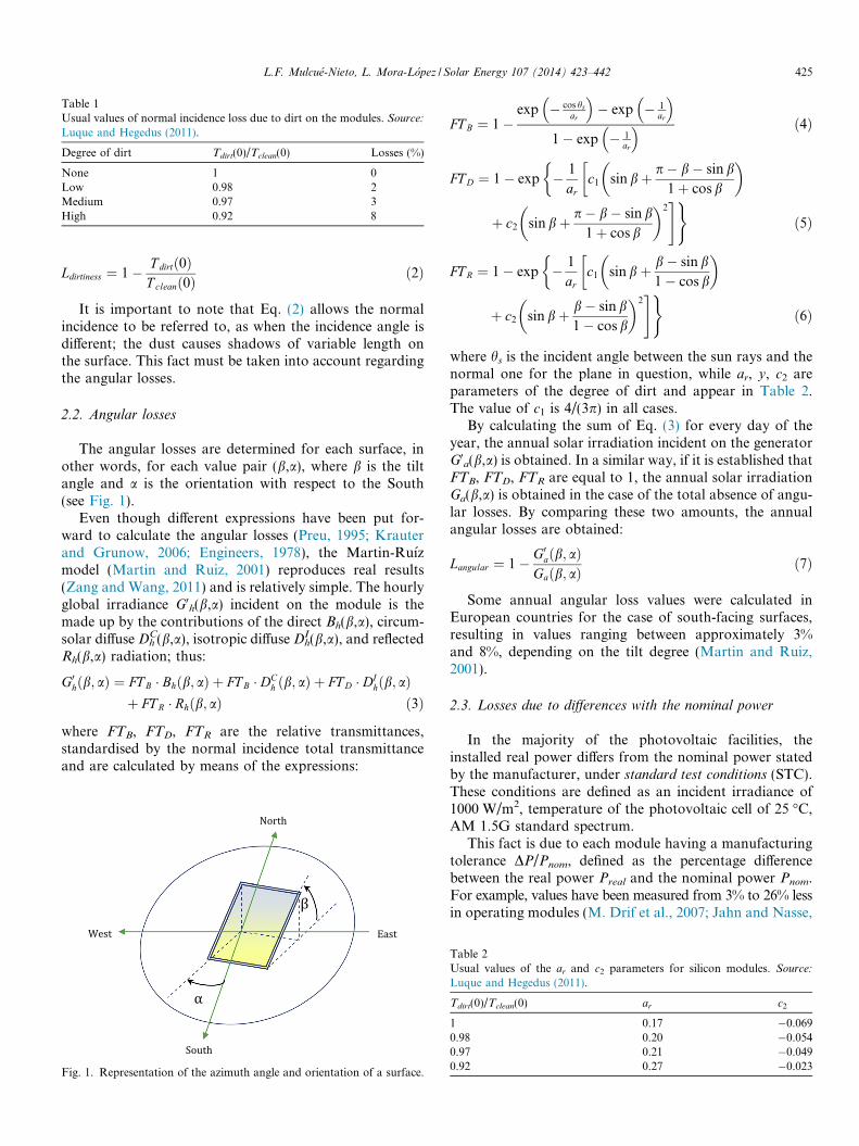
Table 1Usual values of normal incidence loss due to dirt on the modules. Source:

Luque and Hegedus (2011).

Degree of dirt Tdirt(0)/Tclean(0) Losses (%)

None 1 0Low 0.98 2Medium 0.97 3High 0.92 8

L.F. Mulcue-Nieto, L. Mora-Lopez / Solar Energy 107 (2014) 423–442 425

Ldirtiness ¼ 1� T dirtð0ÞT cleanð0Þ

ð2Þ

It is important to note that Eq. (2) allows the normalincidence to be referred to, as when the incidence angle isdifferent; the dust causes shadows of variable length onthe surface. This fact must be taken into account regardingthe angular losses.

2.2. Angular losses

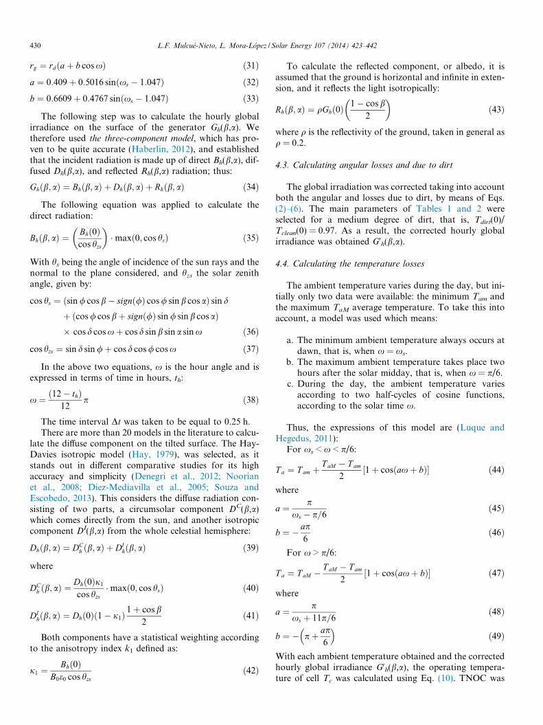
The angular losses are determined for each surface, inother words, for each value pair (b,a), where b is the tiltangle and a is the orientation with respect to the South(see Fig. 1).

Even though different expressions have been put for-ward to calculate the angular losses (Preu, 1995; Krauterand Grunow, 2006; Engineers, 1978), the Martin-Ruızmodel (Martin and Ruiz, 2001) reproduces real results(Zang and Wang, 2011) and is relatively simple. The hourlyglobal irradiance G0h(b,a) incident on the module is themade up by the contributions of the direct Bh(b,a), circum-solar diffuse DC

h (b,a), isotropic diffuse DIh(b,a), and reflected

Rh(b,a) radiation; thus:

G0hðb; aÞ ¼ FT B � Bhðb; aÞ þ FT B � DCh ðb; aÞ þ FT D � DI

hðb; aÞþ FT R � Rhðb; aÞ ð3Þ

where FTB, FTD, FTR are the relative transmittances,standardised by the normal incidence total transmittanceand are calculated by means of the expressions:

Fig. 1. Representation of the azimuth angle and orientation of a surface.

FT B ¼ 1�exp � cos hs

ar

� �� exp � 1

ar

� �1� exp � 1

ar

� � ð4Þ

FT D ¼ 1� exp � 1

arc1 sin bþ p� b� sin b

1þ cos b

� ��

þ c2 sin bþ p� b� sin b1þ cos b

� �2#)

ð5Þ

FT R ¼ 1� exp � 1

arc1 sin bþ b� sin b

1� cos b

� ��

þ c2 sin bþ b� sin b1� cos b

� �2#)

ð6Þ

where hs is the incident angle between the sun rays and thenormal one for the plane in question, while ar, y, c2 areparameters of the degree of dirt and appear in Table 2.The value of c1 is 4/(3p) in all cases.

By calculating the sum of Eq. (3) for every day of theyear, the annual solar irradiation incident on the generatorG0a(b,a) is obtained. In a similar way, if it is established thatFTB, FTD, FTR are equal to 1, the annual solar irradiationGa(b,a) is obtained in the case of the total absence of angu-lar losses. By comparing these two amounts, the annualangular losses are obtained:

Langular ¼ 1� G0aðb; aÞGaðb; aÞ

ð7Þ

Some annual angular loss values were calculated inEuropean countries for the case of south-facing surfaces,resulting in values ranging between approximately 3%and 8%, depending on the tilt degree (Martin and Ruiz,2001).

2.3. Losses due to differences with the nominal power

In the majority of the photovoltaic facilities, theinstalled real power differs from the nominal power statedby the manufacturer, under standard test conditions (STC).These conditions are defined as an incident irradiance of1000 W/m2, temperature of the photovoltaic cell of 25 �C,AM 1.5G standard spectrum.

This fact is due to each module having a manufacturingtolerance DP/Pnom, defined as the percentage differencebetween the real power Preal and the nominal power Pnom.For example, values have been measured from 3% to 26% lessin operating modules (M. Drif et al., 2007; Jahn and Nasse,

Table 2Usual values of the ar and c2 parameters for silicon modules. Source:

Luque and Hegedus (2011).

Tdirt(0)/Tclean(0) ar c2

1 0.17 �0.0690.98 0.20 �0.0540.97 0.21 �0.0490.92 0.27 �0.023


2004; Poissant and CanmetENERGY, 2009; Atmaramet al., 2008; Detrick et al., 2005; Carr and Pryor, 2004).Table 3 summarises some research showing the great dis-persion of this parameter.

The high percentages reported may result in system per-formances of under 60% (Jahn and Nasse, 2004). However,recent studies have concluded that manufacturers areincreasingly more responsible for this situation. Proof ofthis is the research carried out by Solar America Board

for Codes and Standards (“Solar America Board forCodes and Standards (Solar ABCs),” 2013), where 9422modules were reviewed, concluding that less than 0.7% ofthe total presented power under 97% of the nominal power(TamizhMani, 2011).

For a generator consisting of n modules equal to nomi-nal power Pnom, losses due to differences with the nominalpower Lrating are determined by:

Lrating ¼ 1� 1

n

Xn

i¼1

P real;i

P nomð8Þ

where real Preal,i represents the real power of the ithmodule.

If the modules are well selected, the losses due to differ-ences with the nominal power can be estimated as beingequal to 5% as a maximum (Almonacid et al., 2011).

2.4. Mismatch losses

When performing photovoltaic module parallel or serialconnections, experience has shown that the total power ofthe system is not equal to the sum of the individual power.This energy deficit is attributed to the so-called mismatchlosses, which are mainly caused by the partial shading ofthe generator and the dispersion of the electricity proper-ties of the modules (Chouder and Silvestre, 2009).

The electric characteristics of each unit of the generatormay vary due to the manufacturer’s tolerance or degrada-tion processes. The latter includes the degradation of theanti-reflective coating, the discoloration of the housingmaterial, the degradation caused by light, hot points, andthe mechanical breaking of the cell structure (Picaultet al., 2010).

Due to the great many factors intervening in this aspect,there is no simple expression to predict this type of loss.However, there is research that has detected values up to6% due to this concept (Baltus et al., 1997), while other

Table 3Absolute percentage differences between the nominal power issued by the man

Country |DP/Pnom|min (%) |DP/Pnom

Spain 9 11Germany 5 26Canada 6.5 23USA 0 19.7Australia 0.7 25.1

research indicates that they are between 2% and 4%(Almonacid et al., 2011).

2.5. Temperature losses

In the case of monocrystalline silicon modules, the out-put power drops by around 4% for each 10 �C increase intemperature (Luque and Hegedus, 2011). This is mainlydue to the effect of the heating on the open circuit voltageof the photovoltaic cells.

The most common expression to calculate the maximumpower that each module can deliver is the one proposed byOsterwald (1986), as it produces satisfactory results(Almonacid et al., 2011), despite its simplicity. This modeluses the STC conditions as the benchmark:

P max ¼ P max;STCG0ðb; aÞ

GSTC½1þ cðT c � 25Þ� ð9Þ

where Pmax is the maximum power in W, G0(b,a) the inci-dent irradiance on the surface in W/m2, Pmax,STC is themaximum power of the module in STC conditions in W,GSTC = 1000 W/m2, c is the variation coefficient of thepower peak with the temperature, and Tc the instantaneoustemperature of the photovoltaic cells. The latter is given by:

T c ¼ T a þ G0ðb; aÞ TONC � 20

800ð10Þ

where Ta is the ambient temperature and TONC is thenominal operating temperature of the cell, in other words,the one reached in normal incidence conditions under anirradiance equal to 800 W/m2 and ambient temperatureof 20 �C.

Pursuant to the above, the instantaneous temperaturelosses would be given by the difference between the realpower Pmax and the hypothetical power produced if thecells were working at 25 �C, resulting in:

Ltemperature;ins ¼ �cðT c � 25Þ ð11Þ

It can be seen that these losses depend on the tempera-ture of the cells, in other words, of the ambient temperatureand of the incident irradiance on the generator plane. In asimilar way, they are determined for a time period by theexpression proposed Caamano Martın (1998):

Ltemperature ¼ �cðTOE � 25Þ ð12Þ

where TOE is the Equivalent Operating Temperature of thegenerator in the period in question, weighted by the inci-dent irradiance:

ufacturer and the real operating power of the modules.

|max (%) Reference

Drif et al. (2007)Jahn and Nasse (2004)Poissant and CanmetENERGY (2009)Atmaram et al. (2008), Detrick et al. (2005)Carr and Pryor (2004)


TOE ¼R

s T c � G0ðb; aÞ � dtRs G0ðb; aÞ � dt

ð13Þ

It can be seen that these losses are complex to evaluatefor each system in particular, as they depend on the tiltand orientation of the generator, the incident irradianceon the plane of the generator (and therefore also on theangular losses) and the ambient temperature of the place.Typical values range between 5% and 15% (Almonacidet al., 2011).

2.6. Losses due to monitoring errors of the power maximum

peak (PMP)

When the inverter cannot locate the optimal workingpoint of the generator in the current curve–voltage, lossesoccur due to power being generated that is lower thanexpected. These losses depend on external and internal fac-tors to the inverter, including (Jantsch, 1997):

� The PMP monitoring mechanism.� The electrical characteristics of the generator.� The incident irradiance and its irregularities.� The ambient temperature.

Research conducted in 100 residential photovoltaicinstallations in Japan, by the Japanese monitoring pro-gramme, concludes that the average losses due to monitor-ing errors of the power maximum peak LSPMP are of theorder of 6% (Sugiura et al., 2003). This is consistent withdata reported by the Spanish Centre for Technological,Environmental and Energy Research (CIEMAT) (“Centrode Investigaciones Energeticas, Medioambientales yTecnologicas de Espana (CIEMAT),” 2013), with respectto which the standard values range between 4% and 6%for clear days and partially clouded days, respectively(Alonso-Abella and Chenlo, 2004).

2.7. Losses in the inverter due to DC–AC conversion

The DC–AC conversion efficiency of the inverters is thefunction, mainly, of the input power. However, it alsoaffects the value of the input voltage and working temper-ature to a lesser extent. A frequently used model to describethis behaviour is the one proposed by Schmidt, accordingto which the instantaneous efficiency of the inverter is cal-culated by means of the equation (Jantsch et al., 1992):

ginverter ¼P output

P input¼ pout

pout þ k0 þ k1 � pout þ k2 � p2out

ð14Þ

where

pout ¼P output

P nominalð15Þ

Pinput is the instantaneous power at the input of the inverterin W, Poutput is the instantaneous power at the output of theinverter in W, Pnominal is the output nominal power of the

inverter at W, k0 is the self-consumption loss coefficient,k1 is the coefficient of losses proportional to the powerand k2 is the coefficient of losses proportional to the squareof the power. Those parameters can be obtained of the effi-ciency curve of the inverter, provided by the manufacturer.

For simulation purposes, it is better to use an equivalentexpression, but in terms of the input power:

ginverter ¼P output

P input¼ pin � ðb0 þ b1 � pin þ b2 � p2

inÞpin

ð16Þ

where

pin ¼P input

P nominalð17Þ

The values of the normally used coefficients areb0 = 0.02, b1 = 0.02, b2 = 0.07; and are characteristics ofthe inverter type. These values match those of the Schmidtmodel k0 = 0.02, k1 = 0.025, k2 = 0.08; and were calculatedby choosing a representative sample of inverters existing onthe markers (Jantsch et al., 1992).

The aforementioned expression enables the losses in theinverter to be calculated over a period of time s:

Linverter ¼ 1� EAC

EDC¼ 1�

Rs ginverter � P max � dtR

s P maxdtð18Þ

where EAC is the energy generated at the output of theinverter, EDC is the energy generated by the photovoltaicgenerator, and Pmax is given by the Osterwald model(Osterwald, 1986), described above.

In a similar way to the temperature losses, the losses in theinverter depend on the tilt and orientation of the generator,the incident irradiance on the plane of the generator (andtherefore also of the angular losses), the ambient temperatureof the place, and of the inverter type. Therefore, they are verycomplex to assess as they are characteristics of the facility.

Conversion losses have been reported in a wide range.For example, some studies place them at around 13%(Mondol et al., 2006), 9.6–17.5% (Baltus et al., 1997),6.3–16.8% (Alonso-Abella and Chenlo, 2004). However,they can be taken to be equal to 5% for very good inverters(Luque and Hegedus, 2011).

2.8. Ohmic losses in the cabling

The ohmic losses can be calculated approximately for atime period s, by means of the expression:

Lohmic ¼

Xn

i¼1

Rs I i � R2

i � dtRs P maxdt

ð19Þ

where n represents the number of cables, Ii is the current thatcirculates in the i-th cable of electric resistance Ri, and Pmax isgiven by the Osterwald model (Osterwald, 1986).

Usually, these losses fluctuate between 0.5% and 1.5%(Almonacid et al., 2011; Baltus et al., 1997), with 1% beingan acceptable average value to be used.


2.9. Losses due to shading

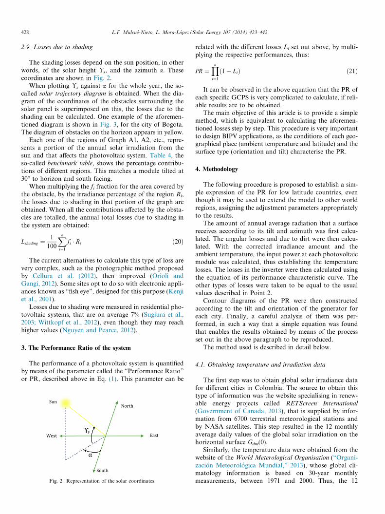
The shading losses depend on the sun position, in otherwords, of the solar height !s, and the azimuth a. Thesecoordinates are shown in Fig. 2.

When plotting !s against a for the whole year, the so-called solar trajectory diagram is obtained. When the dia-gram of the coordinates of the obstacles surrounding thesolar panel is superimposed on this, the losses due to theshading can be calculated. One example of the aforemen-tioned diagram is shown in Fig. 3, for the city of Bogota.The diagram of obstacles on the horizon appears in yellow.

Each one of the regions of Graph A1, A2, etc., repre-sents a portion of the annual solar irradiation from thesun and that affects the photovoltaic system. Table 4, theso-called benchmark table, shows the percentage contribu-tions of different regions. This matches a module tilted at30� to horizon and south facing.

When multiplying the fi fraction for the area covered bythe obstacle, by the irradiance percentage of the region Ri,the losses due to shading in that portion of the graph areobtained. When all the contributions affected by the obsta-cles are totalled, the annual total losses due to shading inthe system are obtained:

Lshading ¼1

100

Xn

i¼1

fi � Ri ð20Þ

The current alternatives to calculate this type of loss arevery complex, such as the photographic method proposedby Cellura et al. (2012), then improved (Orioli andGangi, 2012). Some sites opt to do so with electronic appli-ances known as “fish eye”, designed for this purpose (Kenjiet al., 2001).

Losses due to shading were measured in residential pho-tovoltaic systems, that are on average 7% (Sugiura et al.,2003; Wittkopf et al., 2012), even though they may reachhigher values (Nguyen and Pearce, 2012).

3. The Performance Ratio of the system

The performance of a photovoltaic system is quantifiedby means of the parameter called the “Performance Ratio”

or PR, described above in Eq. (1). This parameter can be

Fig. 2. Representation of the solar coordinates.

related with the different losses Li set out above, by multi-plying the respective performances, thus:

PR ¼Yn

i¼1

ð1� LiÞ ð21Þ

It can be observed in the above equation that the PR ofeach specific GCPS is very complicated to calculate, if reli-able results are to be obtained.

The main objective of this article is to provide a simplemethod, which is equivalent to calculating the aforemen-tioned losses step by step. This procedure is very importantto design BIPV applications, as the conditions of each geo-graphical place (ambient temperature and latitude) and thesurface type (orientation and tilt) characterise the PR.

4. Methodology

The following procedure is proposed to establish a sim-ple expression of the PR for low latitude countries, eventhough it may be used to extend the model to other worldregions, assigning the adjustment parameters appropriatelyto the results.

The amount of annual average radiation that a surfacereceives according to its tilt and azimuth was first calcu-lated. The angular losses and due to dirt were then calcu-lated. With the corrected irradiance amount and theambient temperature, the input power at each photovoltaicmodule was calculated, thus establishing the temperaturelosses. The losses in the inverter were then calculated usingthe equation of its performance characteristic curve. Theother types of losses were taken to be equal to the usualvalues described in Point 2.

Contour diagrams of the PR were then constructedaccording to the tilt and orientation of the generator foreach city. Finally, a careful analysis of them was per-formed, in such a way that a simple equation was foundthat enables the results obtained by means of the processset out in the above paragraph to be reproduced.

The method used is described in detail below.

4.1. Obtaining temperature and irradiation data

The first step was to obtain global solar irradiance datafor different cities in Colombia. The source to obtain thistype of information was the website specialising in renew-able energy projects called RETScreen International(Government of Canada, 2013), that is supplied by infor-mation from 6700 terrestrial meteorological stations andby NASA satellites. This step resulted in the 12 monthlyaverage daily values of the global solar irradiation on thehorizontal surface Gdm(0).

Similarly, the temperature data were obtained from thewebsite of the World Meterological Organisation (“Organi-zacion Meteorologica Mundial,” 2013), whose global cli-matology information is based on 30-year monthlymeasurements, between 1971 and 2000. Thus, the 12

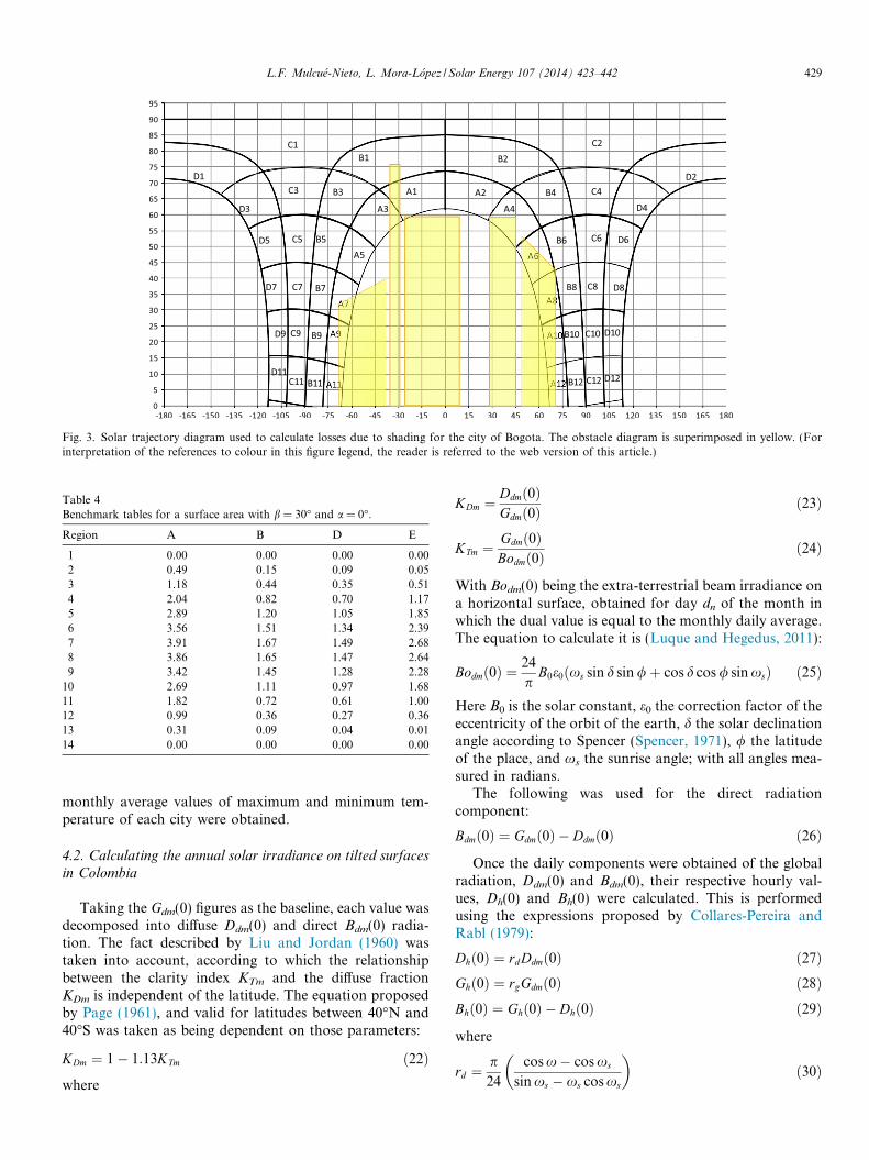
Fig. 3. Solar trajectory diagram used to calculate losses due to shading for the city of Bogota. The obstacle diagram is superimposed in yellow. (Forinterpretation of the references to colour in this figure legend, the reader is referred to the web version of this article.)

Table 4Benchmark tables for a surface area with b = 30� and a = 0�.

Region A B D E

1 0.00 0.00 0.00 0.002 0.49 0.15 0.09 0.053 1.18 0.44 0.35 0.514 2.04 0.82 0.70 1.175 2.89 1.20 1.05 1.856 3.56 1.51 1.34 2.397 3.91 1.67 1.49 2.688 3.86 1.65 1.47 2.649 3.42 1.45 1.28 2.28

10 2.69 1.11 0.97 1.6811 1.82 0.72 0.61 1.0012 0.99 0.36 0.27 0.3613 0.31 0.09 0.04 0.0114 0.00 0.00 0.00 0.00


monthly average values of maximum and minimum tem-perature of each city were obtained.

4.2. Calculating the annual solar irradiance on tilted surfaces

in Colombia

Taking the Gdm(0) figures as the baseline, each value wasdecomposed into diffuse Ddm(0) and direct Bdm(0) radia-tion. The fact described by Liu and Jordan (1960) wastaken into account, according to which the relationshipbetween the clarity index KTm and the diffuse fractionKDm is independent of the latitude. The equation proposedby Page (1961), and valid for latitudes between 40�N and40�S was taken as being dependent on those parameters:

KDm ¼ 1� 1:13KTm ð22Þ

where

KDm ¼Ddmð0ÞGdmð0Þ

ð23Þ

KTm ¼Gdmð0ÞBodmð0Þ

ð24Þ

With Bodm(0) being the extra-terrestrial beam irradiance ona horizontal surface, obtained for day dn of the month inwhich the dual value is equal to the monthly daily average.The equation to calculate it is (Luque and Hegedus, 2011):

Bodmð0Þ ¼24

pB0e0ðxs sin d sin /þ cos d cos / sin xsÞ ð25Þ

Here B0 is the solar constant, e0 the correction factor of theeccentricity of the orbit of the earth, d the solar declinationangle according to Spencer (Spencer, 1971), / the latitudeof the place, and xs the sunrise angle; with all angles mea-sured in radians.

The following was used for the direct radiationcomponent:

Bdmð0Þ ¼ Gdmð0Þ � Ddmð0Þ ð26Þ

Once the daily components were obtained of the globalradiation, Ddm(0) and Bdm(0), their respective hourly val-ues, Dh(0) and Bh(0) were calculated. This is performedusing the expressions proposed by Collares-Pereira andRabl (1979):

Dhð0Þ ¼ rdDdmð0Þ ð27ÞGhð0Þ ¼ rgGdmð0Þ ð28ÞBhð0Þ ¼ Ghð0Þ � Dhð0Þ ð29Þ

where

rd ¼p24

cos x� cos xs

sin xs � xs cos xs

� �ð30Þ


rg ¼ rdðaþ b cos xÞ ð31Þ

a ¼ 0:409þ 0:5016 sinðxs � 1:047Þ ð32Þ

b ¼ 0:6609þ 0:4767 sinðxs � 1:047Þ ð33Þ

The following step was to calculate the hourly globalirradiance on the surface of the generator Gh(b,a). Wetherefore used the three-component model, which has pro-ven to be quite accurate (Haberlin, 2012), and establishedthat the incident radiation is made up of direct Bh(b,a), dif-fused Dh(b,a), and reflected Rh(b,a) radiation; thus:

Ghðb; aÞ ¼ Bhðb; aÞ þ Dhðb; aÞ þ Rhðb; aÞ ð34Þ

The following equation was applied to calculate thedirect radiation:

Bhðb; aÞ ¼Bhð0Þcos hzs

� ��maxð0; cos hsÞ ð35Þ

With hs being the angle of incidence of the sun rays and thenormal to the plane considered, and hzs the solar zenithangle, given by:

cos hs ¼ ðsin / cos b� signð/Þ cos / sin b cos aÞ sin d

þ ðcos / cos bþ signð/Þ sin / sin b cos aÞ� cos d cos xþ cos d sin b sin a sin x ð36Þ

cos hzs ¼ sin d sin /þ cos d cos / cos x ð37Þ

In the above two equations, x is the hour angle and isexpressed in terms of time in hours, th:

x ¼ ð12� thÞ12

p ð38Þ

The time interval Dt was taken to be equal to 0.25 h.There are more than 20 models in the literature to calcu-

late the diffuse component on the tilted surface. The Hay-Davies isotropic model (Hay, 1979), was selected, as itstands out in different comparative studies for its highaccuracy and simplicity (Denegri et al., 2012; Noorianet al., 2008; Diez-Mediavilla et al., 2005; Souza andEscobedo, 2013). This considers the diffuse radiation con-sisting of two parts, a circumsolar component DC(b,a)which comes directly from the sun, and another isotropiccomponent DI(b,a) from the whole celestial hemisphere:

Dhðb; aÞ ¼ DCh ðb; aÞ þ DI

hðb; aÞ ð39Þ

where

DCh ðb; aÞ ¼

Dhð0Þj1

cos hzs�maxð0; cos hsÞ ð40Þ

DIhðb; aÞ ¼ Dhð0Þð1� j1Þ

1þ cos b2

ð41Þ

Both components have a statistical weighting accordingto the anisotropy index k1 defined as:

j1 ¼Bhð0Þ

B0e0 cos hzsð42Þ

To calculate the reflected component, or albedo, it isassumed that the ground is horizontal and infinite in exten-sion, and it reflects the light isotropically:

Rhðb; aÞ ¼ qGhð0Þ1� cos b

2

� �ð43Þ

where q is the reflectivity of the ground, taken in general asq = 0.2.

4.3. Calculating angular losses and due to dirt

The global irradiation was corrected taking into accountboth the angular and losses due to dirt, by means of Eqs.(2)–(6). The main parameters of Tables 1 and 2 wereselected for a medium degree of dirt, that is, Tdirt(0)/Tclean(0) = 0.97. As a result, the corrected hourly globalirradiance was obtained G0h(b,a).

4.4. Calculating the temperature losses

The ambient temperature varies during the day, but ini-tially only two data were available: the minimum Tam andthe maximum TaM average temperature. To take this intoaccount, a model was used which means:

a. The minimum ambient temperature always occurs atdawn, that is, when x = xs.

b. The maximum ambient temperature takes place twohours after the solar midday, that is, when x = p/6.

c. During the day, the ambient temperature variesaccording to two half-cycles of cosine functions,according to the solar time x.

Thus, the expressions of this model are (Luque andHegedus, 2011):

For xs < x < p/6:

T a ¼ T am þT aM � T am

2½1þ cosðaxþ bÞ� ð44Þ

where

a ¼ pxs � p=6

ð45Þ

b ¼ � ap6

ð46Þ

For x > p/6:

T a ¼ T aM �T aM � T am

2½1þ cosðaxþ bÞ� ð47Þ

where

a ¼ pxs þ 11p=6

ð48Þ

b ¼ � pþ ap6

� �ð49Þ

With each ambient temperature obtained and the correctedhourly global irradiance G0h(b,a), the operating tempera-ture of cell Tc was calculated using Eq. (10). TNOC was


taken to be equal to 46 �C, a typical value issued by themodule manufacturers. With this value, and Eq. (9),the output maximum power Pmax was calculated. Thus,the temperature instantaneous losses were established byEq. (11).

4.5. Calculating the losses due to the DC–AC conversion

With the power established in the above point and Eq.(16), the instantaneous efficiency of the inverter was calcu-lated. To discover pin, the nominal Pnominal power of theinverter is assumed to be equal to the peak power of thegenerator Pmax,STC. The output instantaneous power wasthen obtained. The total losses of the DC–AC conversionwere thus calculated using Eq. (18).

4.6. Determining the other types of losses

With respect to the types of remaining losses, they weretaken to be equal to the average values reported in the lit-erature, as set out in Point 2 of this article: Lrating = 0.05,Lmismatch = 0.03, LSPMP = 0.06, Lohmic = 0.01, Lshading =0.07.

Table 5Results obtained for the angular losses.

City Latitude u (�) Langular min (%) Langular max (%)

Leticia �4.2 5 12Pasto 1.2 5 11Tumaco 1.8 4 12Popayan 2.5 5 12Neiva 3 5 12Cali 3.6 5 12Villavicencio 4.2 5 11Bogota 4.7 4 13Manizales 5.1 5 12Medellın 6.2 5 12Barrancabermeja 0.5 4 14Cucuta 7.9 4 13Monterıa 8.8 4 13Valledupar 10.5 4 14Barranquilla 10.9 4 14San Andres 12.6 4 15

4.7. Calculating the PR

The final Performance Ratio was calculated using Eq.(1). Therefore, the annual irradiation Ga(b,a) was givenby means of the average of the monthly average daily val-ues Gdm(b,a), multiplied by 365:

Gaðb; aÞ ¼ 365 � 1

12

X12

n¼1

Gdmðb; aÞ ð50Þ

where the monthly average daily irradiation Gdm(b,a) wasobtained by adding up the hourly components of thehourly global irradiation, during the representative day:

Gdmðb; aÞ ¼Xday

Ghðb; aÞ � Dt ð51Þ

On the other hand, the photovoltaic energy was givenby:

EPV ¼ EACð1� LratingÞð1� LmismatchÞð1� LSPMP Þ� ð1� LohmicÞð1� LshadingÞ ð52Þ

where EAC was calculated to a similar way to Ga(b,a), usingthe equations:

EAC ¼ 365 � 1

12

X12

n¼1

EAC;dm ð53Þ

EAC;dm ¼Xday

ginverter � P max � Dt ð54Þ

The procedure described in points 4.2–4.7 was repeatedcyclically, so that the PR value was obtained for each pairof coordinates (b,a), for the city in question. Tilt b varied

between 0� and 90�, taking Db = 5�; and tilt a between�180� and 180�, taking Da = 5�. All the possible configura-tions could thus be covered.

Finally, the process was repeated for 16 cities of Colom-bia located between latitudes of �4�S and 12�N. Severalother cities in Central America were also taken intoaccount.

5. Results and discussion

5.1. Angular losses and due to dirt

The results of the angular losses for the 16 cities ofColombia are set out in Table 5. It can there be seen thatthe minimum values of this variable range between 4%and 5%, while the maximums are between 11% and 15%.

This behaviour differs slightly from the one reported forsome cities of Europe (Martin and Ruiz, 2001), accordingto which the maximum losses were 8%, for 90� tilt. Thiscan be explained by the fact that the south-facing frontagesin equatorial countries receive less irradiation than thoselocated in high latitudes.

It can also be seen from Table 5 that there is an approx-imate trend of a 1% increase in the maximum losses foreach 3� of latitude. This is logical, as this type of lossescan occur for north-facing vertical surfaces, which receiveless irradiation as the latitude increases.

Fig. 4 was prepared to better understand the behaviourof the south-facing surface angular losses, according totheir tilt angle.

It can be seen from Fig. 4 that the angular lossesincrease with the tilt. However, each curve really presentsa minimum, which is given for the optimum angle thatmaximises the annual global irradiation. This trend canbe better appreciated the greater the latitude of the place.In this case, it is San Andres, whose minimum is approxi-mately for 15�.

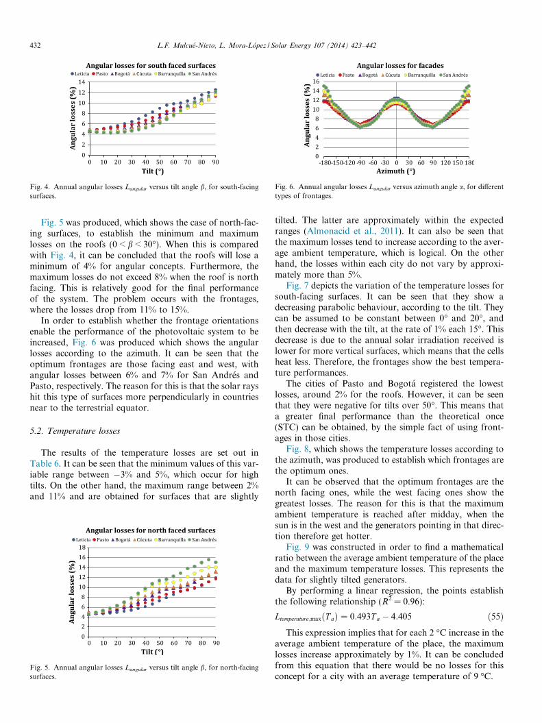
Fig. 4. Annual angular losses Langular versus tilt angle b, for south-facingsurfaces.

Fig. 6. Annual angular losses Langular versus azimuth angle a, for differenttypes of frontages.


Fig. 5 was produced, which shows the case of north-fac-ing surfaces, to establish the minimum and maximumlosses on the roofs (0 < b < 30�). When this is comparedwith Fig. 4, it can be concluded that the roofs will lose aminimum of 4% for angular concepts. Furthermore, themaximum losses do not exceed 8% when the roof is northfacing. This is relatively good for the final performanceof the system. The problem occurs with the frontages,where the losses drop from 11% to 15%.

In order to establish whether the frontage orientationsenable the performance of the photovoltaic system to beincreased, Fig. 6 was produced which shows the angularlosses according to the azimuth. It can be seen that theoptimum frontages are those facing east and west, withangular losses between 6% and 7% for San Andres andPasto, respectively. The reason for this is that the solar rayshit this type of surfaces more perpendicularly in countriesnear to the terrestrial equator.

5.2. Temperature losses

The results of the temperature losses are set out inTable 6. It can be seen that the minimum values of this var-iable range between �3% and 5%, which occur for hightilts. On the other hand, the maximum range between 2%and 11% and are obtained for surfaces that are slightly

Fig. 5. Annual angular losses Langular versus tilt angle b, for north-facingsurfaces.

tilted. The latter are approximately within the expectedranges (Almonacid et al., 2011). It can also be seen thatthe maximum losses tend to increase according to the aver-age ambient temperature, which is logical. On the otherhand, the losses within each city do not vary by approxi-mately more than 5%.

Fig. 7 depicts the variation of the temperature losses forsouth-facing surfaces. It can be seen that they show adecreasing parabolic behaviour, according to the tilt. Theycan be assumed to be constant between 0� and 20�, andthen decrease with the tilt, at the rate of 1% each 15�. Thisdecrease is due to the annual solar irradiation received islower for more vertical surfaces, which means that the cellsheat less. Therefore, the frontages show the best tempera-ture performances.

The cities of Pasto and Bogota registered the lowestlosses, around 2% for the roofs. However, it can be seenthat they were negative for tilts over 50�. This means thata greater final performance than the theoretical once(STC) can be obtained, by the simple fact of using front-ages in those cities.

Fig. 8, which shows the temperature losses according tothe azimuth, was produced to establish which frontages arethe optimum ones.

It can be observed that the optimum frontages are thenorth facing ones, while the west facing ones show thegreatest losses. The reason for this is that the maximumambient temperature is reached after midday, when thesun is in the west and the generators pointing in that direc-tion therefore get hotter.

Fig. 9 was constructed in order to find a mathematicalratio between the average ambient temperature of the placeand the maximum temperature losses. This represents thedata for slightly tilted generators.

By performing a linear regression, the points establishthe following relationship (R2 = 0.96):

Ltemperature;maxðT aÞ ¼ 0:493T a � 4:405 ð55ÞThis expression implies that for each 2 �C increase in the

average ambient temperature of the place, the maximumlosses increase approximately by 1%. It can be concludedfrom this equation that there would be no losses for thisconcept for a city with an average temperature of 9 �C.

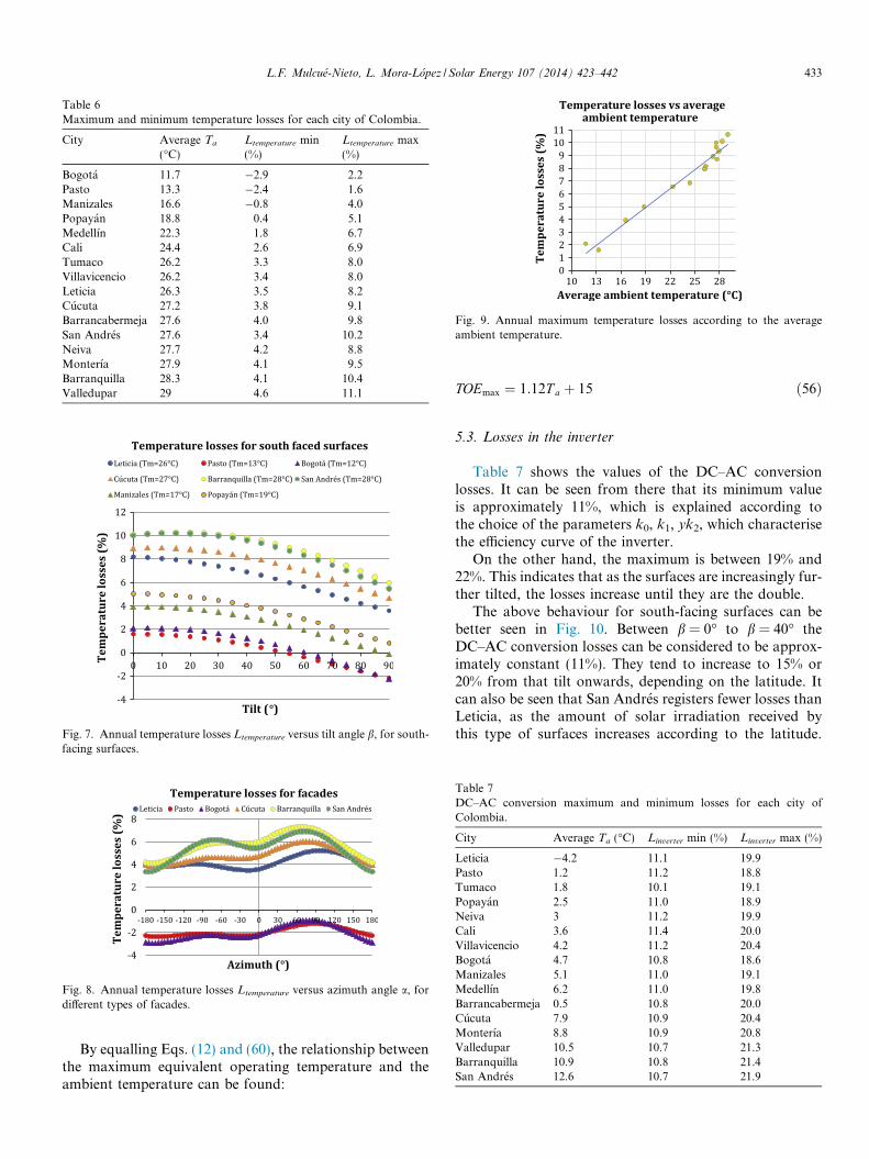
Table 6Maximum and minimum temperature losses for each city of Colombia.

City Average Ta

(�C)Ltemperature min(%)

Ltemperature max(%)

Bogota 11.7 �2.9 2.2Pasto 13.3 �2.4 1.6Manizales 16.6 �0.8 4.0Popayan 18.8 0.4 5.1Medellın 22.3 1.8 6.7Cali 24.4 2.6 6.9Tumaco 26.2 3.3 8.0Villavicencio 26.2 3.4 8.0Leticia 26.3 3.5 8.2Cucuta 27.2 3.8 9.1Barrancabermeja 27.6 4.0 9.8San Andres 27.6 3.4 10.2Neiva 27.7 4.2 8.8Monterıa 27.9 4.1 9.5Barranquilla 28.3 4.1 10.4Valledupar 29 4.6 11.1

Fig. 7. Annual temperature losses Ltemperature versus tilt angle b, for south-facing surfaces.

Fig. 8. Annual temperature losses Ltemperature versus azimuth angle a, fordifferent types of facades.

Fig. 9. Annual maximum temperature losses according to the averageambient temperature.

Table 7DC–AC conversion maximum and minimum losses for each city ofColombia.

City Average Ta (�C) Linverter min (%) Linverter max (%)

Leticia �4.2 11.1 19.9Pasto 1.2 11.2 18.8Tumaco 1.8 10.1 19.1Popayan 2.5 11.0 18.9Neiva 3 11.2 19.9Cali 3.6 11.4 20.0Villavicencio 4.2 11.2 20.4Bogota 4.7 10.8 18.6Manizales 5.1 11.0 19.1Medellın 6.2 11.0 19.8Barrancabermeja 0.5 10.8 20.0Cucuta 7.9 10.9 20.4Monterıa 8.8 10.9 20.8Valledupar 10.5 10.7 21.3Barranquilla 10.9 10.8 21.4San Andres 12.6 10.7 21.9


By equalling Eqs. (12) and (60), the relationship betweenthe maximum equivalent operating temperature and theambient temperature can be found:

TOEmax ¼ 1:12T a þ 15 ð56Þ

5.3. Losses in the inverter

Table 7 shows the values of the DC–AC conversionlosses. It can be seen from there that its minimum valueis approximately 11%, which is explained according tothe choice of the parameters k0, k1, yk2, which characterisethe efficiency curve of the inverter.

On the other hand, the maximum is between 19% and22%. This indicates that as the surfaces are increasingly fur-ther tilted, the losses increase until they are the double.

The above behaviour for south-facing surfaces can bebetter seen in Fig. 10. Between b = 0� to b = 40� theDC–AC conversion losses can be considered to be approx-imately constant (11%). They tend to increase to 15% or20% from that tilt onwards, depending on the latitude. Itcan also be seen that San Andres registers fewer losses thanLeticia, as the amount of solar irradiation received bythis type of surfaces increases according to the latitude.

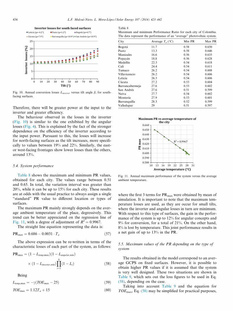
Fig. 10. Annual conversion losses Linverter versus tilt angle b, for south-facing surfaces.

Table 8Maximum and minimum Performance Ratio for each city of Colombia.The data represent the performance of an “average” photovoltaic system.

City Average Ta (�C) Min PR Max PR

Bogota 11.7 0.58 0.650Pasto 13.3 0.58 0.646Manizales 16.6 0.56 0.635Popayan 18.8 0.56 0.628Medellın 22.3 0.54 0.618Cali 24.4 0.54 0.611Tumaco 26.2 0.54 0.608Villavicencio 26.2 0.54 0.606Leticia 26.3 0.54 0.606Cucuta 27.2 0.53 0.604Barrancabermeja 27.6 0.53 0.602San Andres 27.6 0.51 0.599Neiva 27.7 0.54 0.602Monterıa 27.9 0.53 0.601Barranquilla 28.3 0.52 0.599Valledupar 29 0.51 0.597


Therefore, there will be greater power at the input to theinverter and greater efficiency.

The behaviour observed in the losses in the inverter(Fig. 10) is similar to the one exhibited by the angularlosses (Fig. 4). This is explained by the fact of the strongerdependence on the efficiency of the inverter according tothe input power. Pursuant to this, the losses will increasefor north-facing surfaces as the tilt increases, more specifi-cally to values between 19% and 22%. Similarly, the east-or west-facing frontages show lower losses than the others,around 13%.

Fig. 11. Annual maximum performance of the system versus the averageambient temperature.

5.4. System performance

Table 8 shows the maximum and minimum PR values,obtained for each city. The values range between 0.51and 0.65. In total, the variation interval was greater than20%, while it can be up to 15% for each city. These resultsare at odds with the usual practice to always assign a single“standard” PR value to different location or types ofsurfaces.

The maximum PR mainly strongly depends on the aver-age ambient temperature of the place, degressively. Thistrend can be better appreciated on the regression line ofFig. 11, with a degree of adjustment of R2 = 0.9967.

The straight line equation representing the data is:

PRmax ¼ 0:686� 0:0031 � T a ð57Þ

The above expression can be re-written in terms of thecharacteristic losses of each part of the system, as follows:

PRmax ¼ ð1� Ltemp;maxÞð1� Langular;minÞ

� ð1� Linverter;minÞY6

i¼1

ð1� LiÞ ð58Þ

Being

Ltemp;max ¼ �cðTOEmax � 25Þ ð59Þ

TOEmax ¼ 1:12T a þ 15 ð60Þ

where the first 3 terms for PRmax were obtained by mean ofsimulation. It is important to note that the maximum tem-perature losses are used, as they are occur for small tilts,where the inverter and angular losses in turn are minimum.With respect to this type of surfaces, the gain in the perfor-mance of the system is up to 12% for angular concepts and9% for conversion, for a total of 21%. On the other hand,8% is lost by temperature. This joint performance results ina net gain of up to 13% in the PR.

5.5. Maximum values of the PR depending on the type ofsystem

The results obtained in the model correspond to an aver-age GCPS on fixed surfaces. However, it is possible toobtain higher PR values if it is assumed that the systemis very well designed. These two situations are shown inTable 9, which sets out the loss figures to be used in Eq.(58), depending on the case.

Taking into account Table 9 and the equation forTOEmax, Eq. (58) may be simplified for practical purposes,

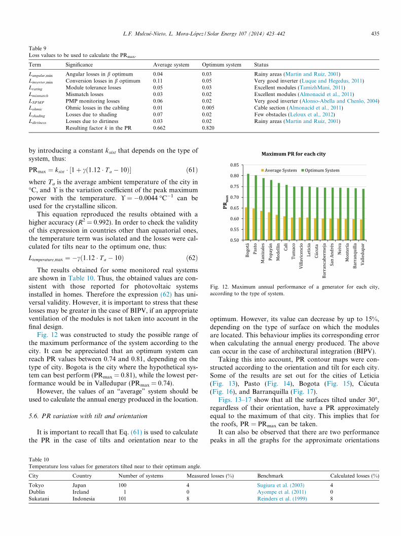
Table 9Loss values to be used to calculate the PRmax.

Term Significance Average system Optimum system Status

Langular,min Angular losses in b optimum 0.04 0.03 Rainy areas (Martin and Ruiz, 2001)Linverter,min Conversion losses in b optimum 0.11 0.05 Very good inverter (Luque and Hegedus, 2011)Lrating Module tolerance losses 0.05 0.03 Excellent modules (TamizhMani, 2011)Lmismatch Mismatch losses 0.03 0.02 Excellent modules (Almonacid et al., 2011)LSPMP PMP monitoring losses 0.06 0.02 Very good inverter (Alonso-Abella and Chenlo, 2004)Lohmic Ohmic losses in the cabling 0.01 0.005 Cable section (Almonacid et al., 2011)Lshading Losses due to shading 0.07 0.02 Few obstacles (Leloux et al., 2012)Ldirtiness Losses due to dirtiness 0.03 0.02 Rainy areas (Martin and Ruiz, 2001)

Resulting factor k in the PR 0.662 0.820

Fig. 12. Maximum annual performance of a generator for each city,according to the type of system.


by introducing a constant ksist that depends on the type ofsystem, thus:

PRmax ¼ ksist � ½1þ cð1:12 � T a � 10Þ� ð61Þ

where Ta is the average ambient temperature of the city in�C, and ! is the variation coefficient of the peak maximumpower with the temperature. ! = �0.0044 �C�1 can beused for the crystalline silicon.

This equation reproduced the results obtained with ahigher accuracy (R2 = 0.992). In order to check the validityof this expression in countries other than equatorial ones,the temperature term was isolated and the losses were cal-culated for tilts near to the optimum one, thus:

Ltemperature;max ¼ �cð1:12 � T a � 10Þ ð62Þ

The results obtained for some monitored real systemsare shown in Table 10. Thus, the obtained values are con-sistent with those reported for photovoltaic systemsinstalled in homes. Therefore the expression (62) has uni-versal validity. However, it is important to stress that theselosses may be greater in the case of BIPV, if an appropriateventilation of the modules is not taken into account in thefinal design.

Fig. 12 was constructed to study the possible range ofthe maximum performance of the system according to thecity. It can be appreciated that an optimum system canreach PR values between 0.74 and 0.81, depending on thetype of city. Bogota is the city where the hypothetical sys-tem can best perform (PRmax = 0.81), while the lowest per-formance would be in Valledupar (PRmax = 0.74).

However, the values of an “average” system should beused to calculate the annual energy produced in the location.

5.6. PR variation with tilt and orientation

It is important to recall that Eq. (61) is used to calculatethe PR in the case of tilts and orientation near to the

Table 10Temperature loss values for generators tilted near to their optimum angle.

City Country Number of systems Measured

Tokyo Japan 100 4Dublin Ireland 1 0Sukatani Indonesia 101 8

optimum. However, its value can decrease by up to 15%,depending on the type of surface on which the modulesare located. This behaviour implies its corresponding errorwhen calculating the annual energy produced. The abovecan occur in the case of architectural integration (BIPV).

Taking this into account, PR contour maps were con-structed according to the orientation and tilt for each city.Some of the results are set out for the cities of Leticia(Fig. 13), Pasto (Fig. 14), Bogota (Fig. 15), Cucuta(Fig. 16), and Barranquilla (Fig. 17).

Figs. 13–17 show that all the surfaces tilted under 30�,regardless of their orientation, have a PR approximatelyequal to the maximum of that city. This implies that forthe roofs, PR = PRmax can be taken.

It can also be observed that there are two performancepeaks in all the graphs for the approximate orientations

losses (%) Benchmark Calculated losses (%)

Sugiura et al. (2003) 4Ayompe et al. (2011) 0Reinders et al. (1999) 8

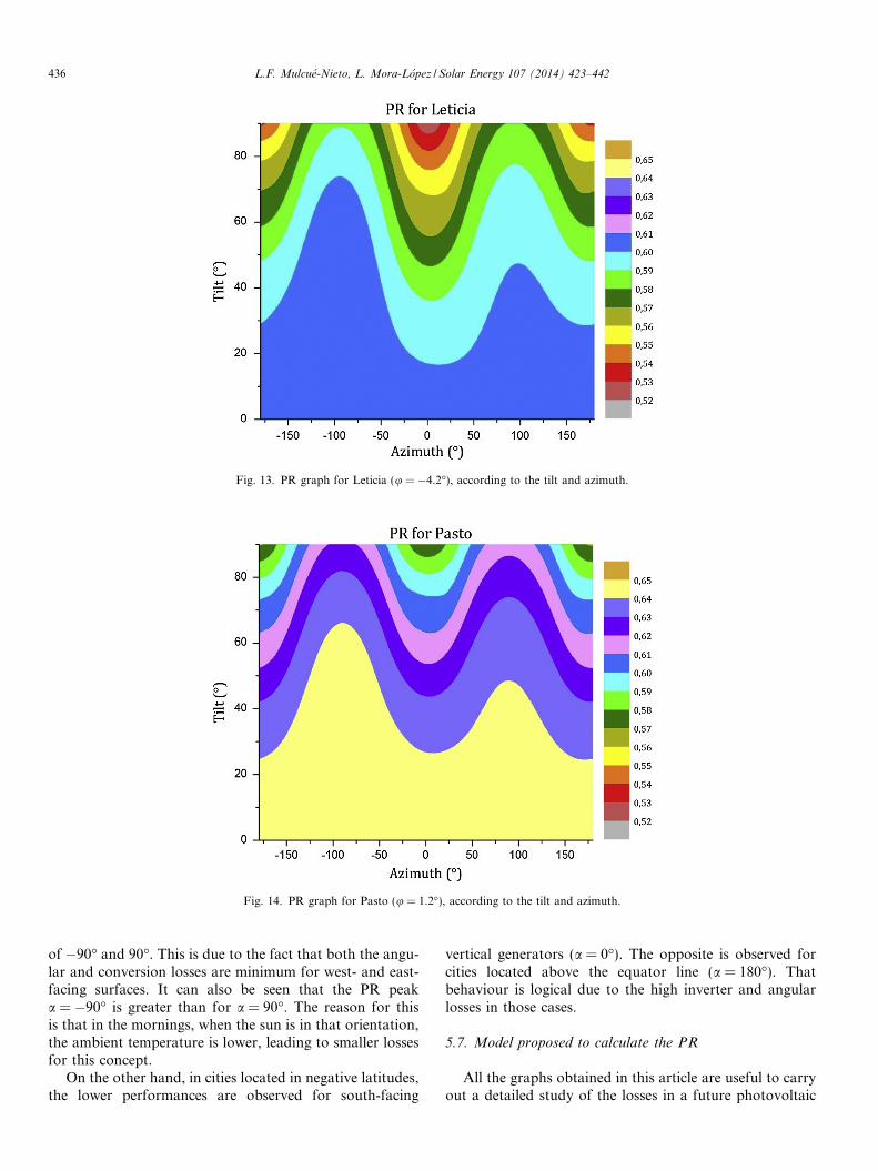
Fig. 13. PR graph for Leticia (u = �4.2�), according to the tilt and azimuth.

Fig. 14. PR graph for Pasto (u = 1.2�), according to the tilt and azimuth.


of �90� and 90�. This is due to the fact that both the angu-lar and conversion losses are minimum for west- and east-facing surfaces. It can also be seen that the PR peaka = �90� is greater than for a = 90�. The reason for thisis that in the mornings, when the sun is in that orientation,the ambient temperature is lower, leading to smaller lossesfor this concept.

On the other hand, in cities located in negative latitudes,the lower performances are observed for south-facing

vertical generators (a = 0�). The opposite is observed forcities located above the equator line (a = 180�). Thatbehaviour is logical due to the high inverter and angularlosses in those cases.

5.7. Model proposed to calculate the PR

All the graphs obtained in this article are useful to carryout a detailed study of the losses in a future photovoltaic

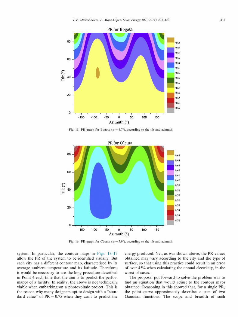
Fig. 15. PR graph for Bogota (u = 4.7�), according to the tilt and azimuth.

Fig. 16. PR graph for Cucuta (u = 7.9�), according to the tilt and azimuth.


system. In particular, the contour maps in Figs. 13–17allow the PR of the system to be identified visually. Buteach city has a different contour map, characterised by itsaverage ambient temperature and its latitude. Therefore,it would be necessary to use the long procedure describedin Point 4 each time that the aim is to predict the perfor-mance of a facility. In reality, the above is not technicallyviable when embarking on a photovoltaic project. This isthe reason why many designers opt to design with a “stan-dard value” of PR = 0.75 when they want to predict the

energy produced. Yet, as was shown above, the PR valuesobtained may vary according to the city and the type ofsurface, so that using this practice could result in an errorof over 45% when calculating the annual electricity, in theworst of cases.

The proposal put forward to solve the problem was tofind an equation that would adjust to the contour mapsobtained. Reasoning in this showed that, for a single PR,the point curve approximately describes a sum of twoGaussian functions. The scope and breadth of such

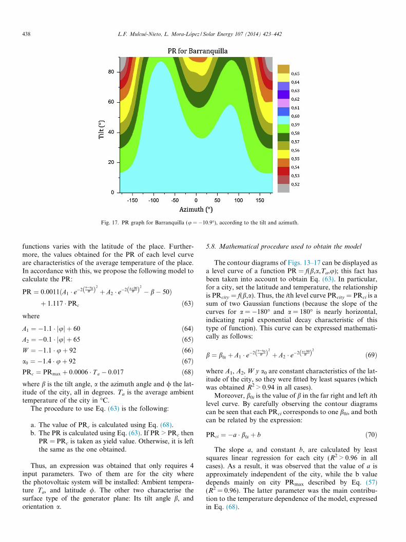
Fig. 17. PR graph for Barranquilla (u = �10.9�), according to the tilt and azimuth.


functions varies with the latitude of the place. Further-more, the values obtained for the PR of each level curveare characteristics of the average temperature of the place.In accordance with this, we propose the following model tocalculate the PR:

PR ¼ 0:0011ðA1 � e�2a�a0

Wð Þ2 þ A2 � e�2 aþ90Wð Þ2 � b� 50Þ

þ 1:117 � PRc ð63Þ

where

A1 ¼ �1:1 � juj þ 60 ð64ÞA2 ¼ �0:1 � juj þ 65 ð65ÞW ¼ �1:1 � uþ 92 ð66Þa0 ¼ �1:4 � uþ 92 ð67ÞPRc ¼ PRmax þ 0:0006 � T a � 0:017 ð68Þwhere b is the tilt angle, a the azimuth angle and / the lat-itude of the city, all in degrees. Ta is the average ambienttemperature of the city in �C.

The procedure to use Eq. (63) is the following:

a. The value of PRc is calculated using Eq. (68).b. The PR is calculated using Eq. (63). If PR > PRc then

PR = PRc is taken as yield value. Otherwise, it is leftthe same as the one obtained.

Thus, an expression was obtained that only requires 4input parameters. Two of them are for the city wherethe photovoltaic system will be installed: Ambient tempera-ture Ta, and latitude /. The other two characterise thesurface type of the generator plane: Its tilt angle b, andorientation a.

5.8. Mathematical procedure used to obtain the model

The contour diagrams of Figs. 13–17 can be displayed asa level curve of a function PR = f(b,a,Ta,u); this fact hasbeen taken into account to obtain Eq. (63). In particular,for a city, set the latitude and temperature, the relationshipis PRcity = f(b,a). Thus, the ith level curve PRcity = PRci is asum of two Gaussian functions (because the slope of thecurves for a = �180� and a = 180� is nearly horizontal,indicating rapid exponential decay characteristic of thistype of function). This curve can be expressed mathemati-cally as follows:

b ¼ b0i þ A1 � e�2a�a0

Wð Þ2 þ A2 � e�2 aþ90Wð Þ2 ð69Þ

where A1, A2, W y a0 are constant characteristics of the lat-itude of the city, so they were fitted by least squares (whichwas obtained R2 > 0.94 in all cases).

Moreover, b0i is the value of b in the far right and left ithlevel curve. By carefully observing the contour diagramscan be seen that each PRci corresponds to one b0i, and bothcan be related by the expression:

PRci ¼ �a � b0i þ b ð70Þ

The slope a, and constant b, are calculated by leastsquares linear regression for each city (R2 > 0.96 in allcases). As a result, it was observed that the value of a isapproximately independent of the city, while the b valuedepends mainly on city PRmax described by Eq. (57)(R2 = 0.96). The latter parameter was the main contribu-tion to the temperature dependence of the model, expressedin Eq. (68).


5.9. Degree of accuracy of the model

Fig. 18 was constructed in order to verify the degree ofaccuracy of the model. This graph shows two PR contourdiagrams, one was produced using the long and tediousprocess described in Point 4, and the other was calculatedusing the proposed equation, both for the city of Bogota.

Likewise, Fig. 19 shows the error percentage at eachpoint of the graph. It can be seen how the error made is under1%. This error increases slightly with the temperatureand latitude. For example, for Tegucigalpa–Guatemala

Fig. 18. Contours of the PR for Bogota, calculated by full simu

Fig. 19. Error percentage in the mod

(u = 14.1�); the error in the majority of the point is 3% or less.These results indicate the excellent degree of accuracy of theproposed model, despite its simplicity.

Finally, the following is described to have an idea of thework saved by using Eq. (63) to calculate PR: To establisheach point of the contour diagram of the left part ofFig. 18, it was necessary to use over 40 equations, in a com-puter algorithm that performed over 20,000 operations. Onthe contrary, only two equations were used at each point ofthe graph in the right of the same figure: that of PRmax,Eq. (61), and the one proposed in our model, Eq. (63).

lation (Left) and by means of the proposed model (Right).

el proposed for the Bogota PR.


6. Conclusions

This paper analyses in detail the possible energy lossesthat impacted the performance of a photovoltaic systemconnected to the grid, placed in an equatorial country.The procedure was carried out for 16 cities of Colombia,for all the possible tilts and orientations of the generatorplane.

The results showed that the angular losses were between4% and 15%. It was also seen that there is an approximatetrend of a 1% increase in the maximum losses for each 3� oflatitude.

Maximum and minimum angular losses on the roofswere calculated, where it was found that they were between4% and 8%. The optimum frontages are those facing eastand west, with angular losses between 6% and 7% forSan Andres and Pasto, respectively.

With respect to the temperature losses, they werebetween �3% and 11%. However, they did not vary byover 5%, approximately, within each city. The maximumlosses occurred for low tilts. It was also seen that the max-imum losses tend to increase by 1% for each 2� in the aver-age ambient temperature of the place. It was found thatthere are no losses for this concept for cities with averagetemperature of 9 �C. On the other hand, they were approx-imately constant on the roofs, and then decreased with theslope, on the basis of 1% each 15�, approximately. There-fore, the frontages provided better performances bytemperature.

The cities of Pasto and Bogota registered the lowestlosses by temperature, around 2% on the rooftops. Therewere negative for tilts over 50�, which means a final perfor-mance greater than the theoretical one can be obtained,simply by using frontages in those cities. It was alsoobserved that that the optimum frontages were east facing.

It was found that the maximum equivalent operatingtemperature of the cells is nearly 15� higher than the ambi-ent temperature. Furthermore an equation was proposedto calculate the maximum temperature losses in any coun-try of the world. This was confirmed using monitored sys-tem data.

DC–AC conversion losses were between 11% and 22%.For south facing generators, they remained approximatelyconstant between b = 0� and b = 40� (11%), to then increaseto 15% or 20%, depending on the latitude. San Andres reg-istered fewer losses than Leticia, as the amount of solar irra-diation received by this type of surfaces increases accordingto the latitude. The behaviour observed in the losses in theinverter was similar to the one exhibited by the angularlosses. Therefore, the east- or west-facing frontages showedlower losses than the others, around 13%.

On the other hand, the performance of an “average sys-tem” in each city was estimated, with PR values of between0.51 and 0.65 being found. Thus, the variation was over20%, while it was up to 15% in each city. These resultsare at odds with the usual practice to assign a single “stan-dard” PR value to different location or types of surfaces.

The maximum PR was mainly found for low tilts, anddepends on the average ambient temperature of the place,degressively. This fact also allowed a highly accurate equa-tion to be found that relate both variables, along with thelosses of each element of the photovoltaic system. Thisequation allows an average GCPS to be distinguished fromanother very well-designed one, by introducing a constantknown as ksist. The result was that an optimum system inColombia can reach PR values between 0.74 and 0.81,depending on the type of city.

All the surfaces tilted under 30�, regardless of their ori-entation, have a PR approximately equal to the maximumof that city. This implies that for the roofs, PR = PRmax

can be taken. Furthermore, the greatest performances ofthe frontages were for west- and east-facing surfaces.

Finally, a simple expression was proposed that allowedthe PR to be estimated with just 4 input parameters: Theaverage ambient temperature of the city, the latitude andthe orientation and tilt angles of the plane of the photovol-taic generator. This model has a high degree of accuracy,and is equivalent to performing a complex simulation,according to the one seen in the methodology.

7. Future research

The proposed model can be extended to high latitudecountries, but the parameters of the equation would needto be adjusted. Future researches in this field could includethe analysis of the influence of ground conditions on theBIPV’s surface temperature of PV cells.

We expect the results obtained in this study to be highlyuseful for architects and engineers involved in designingphotovoltaic systems for BIPV in low latitude countries.

Acknowledgements

This research was carried out thanks to the supportreceived by means of a grant from the Universidad Inter-nacional de Andalucıa for studies on the Official Master’sin Technology of the Photovoltaic Solar Energy Systems.Also to the Faculty of Engineering and Architecture ofthe Universidad Catolica de Manizales.

References

Almonacid, F., Rus, C., Perez, P.J., Hontoria, L., 2009. Estimation of theenergy of a PV generator using artificial neural network. Renew.Energy 34, 2743–2750.

Almonacid, F., Rus, C., Perez-Higueras, P., Hontoria, L., 2011. Calcu-lation of the energy provided by a PV generator. Comparative study:conventional methods vs. artificial neural networks. Energy 36, 375–384.

Alonso-Abella, M., Chenlo, F., 2004. A model for energy productionestimation of PV grid connected systems based on energetic losses andexperimental data on site diagnosis. In: 19th European PhotovoltaicSolar Energy Conference, Paris, pp. 2447–2450.

Araujo, G.L., Sanchez, E., Martı, M., 1982. Determination of the two-exponential solar cell equation parameters from empirical data. Sol.Cells 5, 199–204.

http://refhub.elsevier.com/S0038-092X(14)00226-6/h0005











Atmaram, G.H., TamizhMani, G., Ventre, G.G., 2008. Need for uniformphotvoltaic module performance testing and ratings. In: 33rd IEEEPhotovoltaic Specialists Conference, 2008. PVSC ’08. Presented at the33rd IEEE Photovoltaic Specialists Conference, 2008. PVSC ’08, pp.1–6.

Ayompe, L.M., Duffy, A., McCormack, S.J., Conlon, M., 2011. Measuredperformance of a 1.72 kW rooftop grid connected photovoltaic systemin Ireland. Energy Convers. Manage. 52, 816–825.

Baltus, C.W.A., Eikelboom, J.A., Zolingen, R.J.C.V., 1997. Analyticalmonitoring of losses in PV systems. In: 14th European PhotovoltaicSolar Energy Conference. Barcelona.

Caamano Martın, E., 1998. Edificios fotovoltaicos conectados a la redelectrica: caracterizacion y analisis (PhD). E.T.S.I. Telecomunicacion(UPM).

Carr, A., Pryor, T., 2004. A comparison of the performance of differentPV module types in temperate climates. Sol. Energy 76, 285–294.

Cellura, M., Di Gangi, A., Orioli, A., 2012. A photographic method toestimate the shading effect of obstructions. Sol. Energy 86, 886–902.

Centro de Investigaciones Energeticas, Medioambientales y Tecnologicasde Espana (CIEMAT), 2013. [WWW Document]. <http://www.cie-mat.es/>.

Chouder, A., Silvestre, S., 2009. Analysis model of mismatch power lossesin PV systems. J. Sol. Energy Eng. 131, 024504–024504.

Collares-Pereira, M., Rabl, A., 1979. The average distribution of solarradiation-correlations between diffuse and hemispherical and betweendaily and hourly insolation values. Sol. Energy 22, 155–164.

Denegri, M.J., Raichijk, C., Gallegos, H.G., 2012. Evaluacion dediferentes modelos utilizados para la estimacion de la radiacionfotosinteticamente activa en planos inclinados. Av. En Energ. Renov.Medio Ambiente 16, 9–15.

Detrick, A., Kimber, A., Mitchell, L., 2005. Performance evaluationstandards for photovoltaic modules and systems. In: ConferenceRecord of the Thirty-First IEEE Photovoltaic Specialists Conference,2005. Presented at the Conference Record of the Thirty-first IEEEPhotovoltaic Specialists Conference, 2005, pp. 1581–1586.

Diez-Mediavilla, M., de Miguel, A., Bilbao, J., 2005. Measurement andcomparison of diffuse solar irradiance models on inclined surfaces inValladolid (Spain). Energy Convers. Manage. 46, 2075–2092.

Engineers, A.S. of H., 1978. Refrigerating and Air-Conditioning, ASH-RAE Standard Methods of Testing to Determine the ThermalPerformance of Solar Collectors. ASHRAE.

Government of Canada, 2013. N.R.C., RETScreen International. [WWWDocument]. <http://www.retscreen.net/ (accessed 24.08.13).

Green, M.A., 1998. Solar Cells: Operating Principles, Technology andSystem Applications. University of New South Wales.

Haberlin, H., 2012. Photovoltaics: System Design and Practice. JohnWiley & Sons, United Kingdom.

Hay, J.E., 1979. Study of Shortwave Radiation on Non-horizontalSurfaces. Atmospheric Environ. Serv. Report No. 79–12.

Jahn, U., Nasse, W., 2004. Operational performance of grid-connected PVsystems on buildings in Germany. Prog. Photovolt. Res. Appl. 12, 441–448.

Jantsch, M., Schmidt, H., Schmid, 1992. Results on the concerted actionon power conditioning and control. In: 11th European PhotovoltaicSolar Energy Conference. Montreux, pp. 1589–1592.

Jantsch, M., Real, M., Haberlin, H., Whitaker, K., Blasser, G., Kremer,P., Verhoeve, C.W.G., 1997. Measurement of PV maximum powerpoint tracking performance. In: Technical Committee 82: Photo-voltaics. International Electrotechnical Commission, Barcelona.

Kanters, J., Horvat, M., 2012. Solar energy as a design parameter in urbanplanning. Energy Procedia 30, 1143–1152.

Kenji, O., Koichi, S., Kazuhiko, K., 2001. Shading loss analysis of PVsystems using fisheye photography. Pap. Tech. Meet. Front. Technol.Eng. IEE Jpn. FTE-01, 23–28.

Krauter, S., Grunow, P., 2006. Optical modelling and simulation of PVmodule encapsulation to improve structure and material properties formaximum energy yield. In: Conference Record of the 2006 IEEE 4thWorld Conference on Photovoltaic Energy Conversion. Presented at

the Conference Record of the 2006 IEEE 4th World Conference onPhotovoltaic, Energy Conversion, pp. 2133–2137.

Leloux, J., Narvarte, L., Trebosc, D., 2012. Review of the performance ofresidential PV systems in France. Renew. Sustain. Energy Rev. 16,1369–1376.

Liu, B.Y.H., Jordan, R.C., 1960. The interrelationship and characteristicdistribution of direct, diffuse and total solar radiation. Sol. Energy 4,1–19.

Luque, A., Hegedus, S., 2011. Handbook of Photovoltaic Science andEngineering, second ed. Wiley, United Kingdom.

M. Drif, P.J.P., Aguilera, J., Almonacid, G., Gomez, P., de la Casa, J.,Aguilar, J.D., 2007. Univer Project. A grid connected photovoltaicsystem of 200 kW p at Jaen University. Overview and performanceanalysis. Sol. Energy Mater. Sol. Cells 91, 670–683.

Markvart, T., Castaner, L., 2003. Practical Handbook of Photovoltaics:Fundamentals and Applications. Elsevier.

Martin, N., Ruiz, J.M., 2001. Calculation of the PV modules angularlosses under field conditions by means of an analytical model. Sol.Energy Mater. Sol. Cells 70, 25–38.

Mondol, J.D., Yohanis, Y., Smyth, M., Norton, B., 2006. Long termperformance analysis of a grid connected photovoltaic system inNorthern Ireland. Energy Convers. Manage. 47, 2925–2947.

Nguyen, H.T., Pearce, J.M., 2012. Incorporating shading losses in solarphotovoltaic potential assessment at the municipal scale. Sol. Energy86, 1245–1260.

Noorian, A.M., Moradi, I., Kamali, G.A., 2008. Evaluation of 12 modelsto estimate hourly diffuse irradiation on inclined surfaces. Renew.Energy 33, 1406–1412.

Organizacion Meteorologica Mundial, 2013. [WWW Document]. <http://wwis.aemet.es/>.

Orioli, A., Gangi, A.D., 2012. An improved photographic methodto estimate the shading effect of obstructions. Sol. Energy 86, 3470–3488.

Osterwald, C.R., 1986. Translation of device performance measurementsto reference conditions. Sol. Cells 18, 269–279.

Page, J., 1961. The estimation of monthly ea values of daily total shortwave radiation on vertical and inclined surfaces from sunshine recordsfor latitudes 40�N–40�S. In: Proc. UN Conf. New Sources Energy, vol.4, pp. 378–390.

Pearce, J.M., 2002. Photovoltaics—a path to sustainable futures. Futures34, 663–674.

Picault, D., Raison, B., Bacha, S., de la Casa, J., Aguilera, J., 2010.Forecasting photovoltaic array power production subject to mismatchlosses. Sol. Energy 84, 1301–1309.

Poissant, Y., CanmetENERGY, 2009. Field Assessment of novel PVmodule technologies in Canada. In: Presented at the Proc. 4thCanadian Solar Buildings Conference, Proc. 4th Canadian SolarBuildings Conference.

Preu, R., 1995. PV-module reflection losses: measurement, simulation andinfluence on energy yield and performance ratio. In: ThirteenthEuropean Photovoltaic Solar Energy Conference 1995. Proceedings,vol. 2. pp. 1465–1468.

Reinders, A.H.M.E., Pramusito, Sudradjat, A., van Dijk, V.A.P., Muly-adi, R., Turkenburg, W.C., 1999. Sukatani revisited: on the perfor-mance of nine-year-old solar home systems and street lighting systemsin Indonesia. Renew. Sustain. Energy Rev. 3, 1–47.

Roberts, S., Guariento, N., 2009. Building Integrated Photovoltaics: AHandbook. Springer, Switzerland.

Rodrigo, P., Rus, C., Almonacid, F., Perez-Higueras, P.J., Almonacid, G.,2012. A new method for estimating angular, spectral and lowirradiance losses in photovoltaic systems using an artificial neuralnetwork model in combination with the Osterwald model. Sol. EnergyMater. Sol. Cells 96, 186–194.

Senado de la Republica de Colombia, 2003. Ley 855 de 2003. Definicionde Zonas No Interconectadas al SIN.

Solar America Board for Codes and Standards (Solar ABCs) [WWWDocument], 2013. <http://www.solarabcs.org/>.









http://www.ciemat.es/

http://www.ciemat.es/













http://www.retscreen.net/



































http://wwis.aemet.es/

http://wwis.aemet.es/






















http://www.solarabcs.org/


de Souza, A.P., Escobedo, J.F., 2013. Estimates of hourly diffuse radiationon tilted surfaces in Southeast of Brazil. Int. J. Renew. Energy Res.IJRER 3, 207–221.

Spencer, J.W., 1971. Fourier series representation of the position of thesun. Search 2 (5), 172.

Sugiura, T., Yamada, T., Nakamura, H., Umeya, M., Sakuta, K.,Kurokawa, K., 2003. Measurements, analyses and evaluation ofresidential PV systems by Japanese monitoring program. Sol. EnergyMater. Sol. Cells 75, 767–779.

TamizhMani, G., 2011. Solar ABCs Policy Recommendation: ModulePower Rating Requirements.

The International Electrotechnical Commission (IEC), 1998. IEC 61724–1998, Photovoltaic system performance monitoring – Guidelines formeasurement, data exchange and analysis.

Thomas, R., 2012. Photovoltaics and Architecture. Taylor & Francis,London.

Wittkopf, S., Valliappan, S., Liu, L., Ang, K.S., Cheng, S.C.J., 2012.Analytical performance monitoring of a 142.5 kWp grid-connectedrooftop BIPV system in Singapore. Renew. Energy 47, 9–20.

Zang, J., Wang, Y., 2011. Analysis of computation model of particledeposition on transmittance for photovoltaic panels. Energy Procedia12, 554–559.



















a new model to predict the energy generated by a photovoltaic system connected to the grid in low...

Documents