A new metric for evaluating semantic segmentation:leveraging global and contour accuracy

Eduardo Fernandez-Moral1, Renato Martins1, Denis Wolf2, and Patrick Rives1

Abstract— Semantic segmentation of images is an importantproblem for mobile robotics and autonomous driving becauseit offers basic information which can be used for complexreasoning and safe navigation. Different solutions have beenproposed for this problem along the last two decades, and arelevant increment on accuracy has been achieved recently withthe application of deep neural networks for image segmentation.One of the main issues when comparing different neuralnetworks architectures is how to select an appropriate metricto evaluate their accuracy. Furthermore, commonly employedevaluation metrics can display divergent outcomes, and thusit is not clear how to rank different image segmentationsolutions. This paper proposes a new metric which accountsfor both global and contour accuracy in a simple formulationto overcome the weaknesses of previous metrics. We show withseveral examples the suitability of our approach and presenta comparative analysis of several commonly used metrics forsemantic segmentation together with a statistical analysis oftheir correlation. Several network segmentation models areused for validation with virtual and real benchmark imagesequences, showing that our metric captures information of themost commonly used metrics in a single scalar value.

I. INTRODUCTION

The problem of semantic segmentation consists of associ-ating a class label to each pixel of a given image, resulting inanother image of semantic labels, as shown in figs. 1a and 1b.This problem of image understanding is highly relevant inthe context of mobile robotics and autonomous vehicles, forwhich accurate information of the objects in the scene maybe applied for decision making or safe and robust navigationamong others [1].

Semantic segmentation has seen a rapid progress over thepast decade. Recent advances achieved by training differenttypes of Convolutional Neural Networks (CNN) have im-proved notably the accuracy of state-of-the-art techniques[2], [3], [4], [5], [6], [7], [8]. Among the many CNN architec-tures available, convolutional encoder-decoder networks areparticularly well adapted to the problem of pixel labeling.The encoder part of the network creates a rich feature maprepresenting the image content and the decoder transformsthe feature map into a map of class probabilities for everypixel of the input image. Such operation takes into accountthe pooling indices to upsample low resolution features intothe original image resolution. The advantages of this class ofnetwork were presented in [5], [6]. The approach in [6] waslater extended to a Bayesian framework in [7] to provide the

1Lagadic team. INRIA Sophia Antipolis - Mediterranee.2004 Route des Lucioles - BP 93, 06902 Sohpia Antipolis,France. Email: eduardo.fernandez-moral@inria.fr,renato-jose.martins@inria.fr, patrick.rives@inria.fr

2 University of Sao Paulo - ICMC/USP, Brazil. denis@icmc.usp.br

(a) Colour image

(b) Annotated image of classes

(c) Image of class borders (θ = 5)

Fig. 1: Extraction of class borders from an annotated imageof labels from the Virtual KITTI dataset [12].

probabilities associated to the pixel labels. Apart from end-to-end CNNs, Conditional Random Fields (CRFs) have alsobeen used for scene semantic segmentation [9], [3], [10].In [11], a CNN model is used to extract features which arefeed to a Support Vector Machine-based CRF to increase theaccuracy of image segmentation.

The recent availability of 3D range sensors and RGB-Dcameras has also been exploited for semantic segmentation[13], [2], [14], [8]. An initial exploration of adding geometricinformation besides color (e.g., depth images) was addressedin [13], but the global accuracy improvement was marginal.Later, [2] presented an approach where depth information isencoded into images containing horizontal disparity, heightabove the ground and angle with gravity, which outperformsprevious solutions using raw depth for indoor scenes. Adifferent strategy for the same problem is presented in [8],which proposes to fuse depth features and color features inthe encoder part of an encoder-decoder network. AnotherCNN-based approach for joint pixel-wise prediction of se-mantic labels, depth and surface normals was presented in[15].

The appearance of public datasets and benchmarks forsemantic segmentation, both from virtual and real scenarios

[16], [12], [17], facilitates the comparison of solutions, andpromotes the standardization of comparison metrics. Still, thechoice of the most appropriate metrics to evaluate semanticsegmentation is a problem itself, which gains relevance withthe increase of performance and complexity of semanticsegmentation techniques.

A. Contribution

In this paper, we investigate the problem of finding asingle accuracy metric that accounts for both global pixelclassification and good contour segmentation. We proposea new metric based on [18] and [19] which makes use ofthe Jaccard index to account for boundary points with acandidate match belonging to the same class in the targetimage. As we show in our experiments, this metric blendsthe characteristics of the Jaccard index (which is the de factostandard in semantic segmentation) and the border metric BFin a simple formulation, thus allowing to compare easily theoutputs of different segmentation solutions.

B. Outline

The reminder of the paper is organized as follows. SectionII-A reviews related works. In section II-B, we introduce thetraditionally used segmentation evaluation metrics and theirlimitations. Section III describes our proposed metric. Wepresent the different CNN architectures and the experimentalresults in section IV, considering simulated and real bench-mark image sequences, such as the virtual KITTI and KITTI.Finally, in section VI, we draw conclusions and highlightfuture improvements and perspectives.

II. SEMANTIC SEGMENTATION METRICS

In this section, we review some recent related works andthe background on commonly used evaluation metrics forsemantic segmentation.

A. Related works

Comparing the accuracy of different semantic segmenta-tion approaches is commonly carried out through differentglobal and class-wise statistics, such as, global precision,class-wise precision, confusion matrix, F-measure or theJaccard index (also called “intersection over union”). Thesemetrics are described in more detail in section II-B. Globalmetrics like the precision may be a good indicator to evaluatedifferent solutions when the different semantic categorieshave a similar relevance (both in terms of frequency ofappearance and practical importance). But this is not thecase in most applications, where objects which have fewerpixels may be significantly more relevant than others (e.g.,“traffic light” or “cyclist” classes versus the “sky” in thecontext of autonomous vehicles). On the other hand, class-wise metrics (e.g., [6], [8]) avoid the previous limitation,but computing accuracies for each class individually meansthat we cannot compare different segmentation solutionsdirectly (without specifying quantitatively the relevance ofeach class). An alternative metric is to average the chosenclass-wise metric m according to the total number of classes

n (e.g., m = ∑ni=1 mi/n). This class-wise average is less

affected by imbalanced class frequencies than global metrics.Another relevant aspect when evaluating segmentation ap-

proaches is to measure the quality of the segmentation aroundclass contours. [20] proposes to measure the ratio betweencorrect and wrong classified pixels in a region surroundingthe class boundaries, instead of considering all image pixels.Other contour-based metrics include the Berkeley contourmatching score [18], the boundary-based evaluation [21] andthe contour-based score [19]. All these measures are basedon the matching between the class boundaries in the groundtruth and the segmented images. [21] computes the meanand standard deviation of a boundary distance distributionbetween pairs of boundary images. [18] computes the F1-measure from precision and recall values using a distanceerror tolerance θ to decide whether a boundary point has amatch or not. [19] proposes an adaptation of [18] to multi-class segmentation, where the score (BF) is computed asthe average of F1 scores over the classes present in thesegmented image.

The trade-off between global and contour segmentation isan important issue since both: a high rate of correctly labeledpixels and a good contour segmentation are desirable. Forinstance, in the context of autonomous navigation, we areinterested in segmenting accurately the borders of the roadand sidewalk in order to delimit the navigable space for eachagent. In [19], the authors suggest to use both the Jaccardindex and BF as accuracy metrics to capture different aspectsof the segmentation quality (global and contour). However,when the problem consists in ranking different segmentationapproaches based on their results, it is required to rely ona single measure so that different solutions can be directlycompared. This problem is highly relevant, for instance,while using CNNs for semantic segmentation, because we areoften interested in finding the set of hyperparameters whichproduce the best accuracy. This requires the comparison ofmultiple models using a single score. Besides, accuracy met-rics which are also influenced by the quality of boundariesare interesting as loss functions to train the segmentationmodels.

B. Standard accuracy metrics

This section describes the most common metrics used forsemantic segmentation. For reference, a general analysis ofaccuracy metrics for classification tasks can be found in [22].

The “accuracy”, or the ratio of the correctly classifiedelements over all available elements can be calculated asfollows:

Accuracy =TP+TN

TP+TN+FP+FN, (1)

whose notation is detailed in table I.The “precision”, or positive predictive value (PPV), is the

relation between true positives and all elements classified aspositives:

Precision =TP

TP+FP. (2)

TABLE I: Class confusion matrix and notation.

Predicted classPositive Negative

True class Positive True Positive (TP) False Negative (FN)Negative False Positive (FP) True Negative (TN)

The “Recall”, or true positive value (TPV), is the relationbetween true positives and all positive elements:

Recall =TP

TP+FN. (3)

The F-measure [23] is a widely used metric to evaluateclassification results, which consists of the harmonic meanof precision (2) and recall (3) metrics:

Fβ =(β 2 +1)TP

(β 2 +1)TP+β 2FN+FP(4)

where β is scaling between the precision and recall. Consid-ering β = 1, leads to the widely used F1-measure:

F1 =2TP

2TP+FN+FP. (5)

Another common metric to evaluate the results of classi-fication is the Jaccard index (JI):

JI =TP

TP+FN+FP. (6)

Global accuracy metrics are not appropriate evaluationmeasures when class frequencies are unbalanced, which isthe case in most scenarios both in real indoor and outdoorscenes, since they are biased by the dominant classes. Toavoid this, the metrics above are usually evaluated per-class,and their result is averaged over the total amount of classes.

The confusion matrix (C), is a squared matrix where eachcolumn represents the instances in a predicted class whileeach row represents the instances in an actual class. Thus,a value Ci j represents the elements of the class i which areclassified as the class j:

Ci j = |Sigt ◦S j

ps| (7)

where Sigt and S j

ps are the binarized maps of the ground truthclass i and predicted class j respectively, (◦) represents theelement-wise product and (| · |) is the L1 norm. Note that theconfusion matrix is also useful to compute the above metricsin a class-wise manner, e.g.:

JIk =Ckk

∑ni=1 Cik +∑

nj=1 Ck j−Ckk

. (8)

III. A NEW METRIC FOR SUPERVISEDSEGMENTATION

This section describes a new metric for supervised seg-mentation which measures jointly the quality of the seg-mented regions and their boundaries. Our metric is inspiredby the BF score presented in [19], which is defined asfollows. Let’s call Bc

gt the boundary of the binary map ofthe Sc

gt of class c in the ground truth and likewise, Bcps for

its predicted segmentation. For a given distance threshold θ ,the precision for class c is defined as:

Pc =1|Bc

ps|∑

x∈Bcps

[[d(x,Bcgt)< θ ]] (9)

and the recall

Rc =1|Bc

gt |∑

x∈Bcgt

[[d(x,Bcps)< θ ]] (10)

with [[·]] the Iversons bracket notation, where [[z]] = 1 ifz=true and 0 otherwise, and d(·) the Euclidean distancemeasured in pixels. The Fc

1 measure for class c is given by:

BFc = Fc1 =

2 ·Pc ·Rc

Pc +Rc . (11)

The BF in (11) has two main drawbacks. Firstly, it disre-gards the content of the segmentation beyond the thresholddistance θ under which boundaries are matched. Secondly,the results of this metric depends on a discrete filteringof the distribution of boundary distances, so that the samescore is obtained for different segmentations (with differentperceptual quality) as far as the same amount of boundarypixels are within the distance θ . This is shown in tableII, which shows different infra and over-segmentations withtheir corresponding scores.

In order to handle these shortcomings, we compute thedistances from the boundary binary map to the binary mapof the predicted segmentation Bc

gt → Scps for a given class

c to obtain the amount of true positives (TPcBgt

) and falsenegatives (FNc). Similarly, we compute the distance from theboundary of the predicted segmentation to the binary map ofthe ground truth Bc

ps→ Scgt for class c to obtain the amount

of true positives (TPcBps

) and false positives (FPc). The totalnumber of true positives is defined as (TPc = TPc

Bgt+TPc

Bps).

Note that while the BF measure is based on boundary-to-boundary matches, our proposed BJ score is boundary-to-object. To avoid the second shortcoming, we propose tomeasure the values above with a continuous measure of theboundary distances, so that the following values are defined:

TPcBgt = ∑

x∈Bcgt

z with z=

{1− (d(x,Sc

ps)/θ)2 if d(x,Scps)< θ

0 otherwise.(12)

FNc = |Bcgt |−TPc

Bgt (13)

TPcBps = ∑

x∈Bcps

z with z=

{1− (d(x,Sc

gt)/θ)2 if d(x,Scgt)< θ

0 otherwise.(14)

FPc = |Bcps|−TPc

Bps (15)

Then, the score for class c, which we call Boundary Jaccard(BJc) is defined according to the Jaccard index:

BJc =TPc

TPc +FPc +FNc . (16)

This new score is not zero when the ground truth andthe predicted segmentation for a given class have some

TABLE II: Examples of infra-segmentation and over-segmentation of a pedestrian from the Cityscapes dataset. The groundtruth corresponds to figure in the center.

0 .12 .45 .64 .86 ← JI → .88 .77 .66 .54 .300 0 0 0 .99 ← BF → .99 0 0 0 00 .20 .46 .47 .77 ← BJ → .79 .64 .50 .50 .48

Fig. 2: Per-class scores of the segmented circle (top-right) fordifferent levels of infra/over segmentation. The parameter θ

is set to 4 pixels for both BF and BJ, which corresponds to0.0075 of the image diagonal.

overlapping (|Scgt ∪ Sc

gt | > 0 ⇒ BJc > 0). This behavior issimilar for the metric JIc but not for BFc. On the other hand,the BJc score increases when the boundaries of ground truthand predicted segmentation get closer, like for BFc, but witha more continuous behavior than the latter. Figure 2 shows anexample to illustrate the behavior of the metrics BJc, BFc andJIc for different levels of infra/over segmentation, as showedin table II.

Finally, in order to compute the per-image BJ score, weaverage the BJc scores over all the classes present either inthe ground truth or in the predicted segmentation. The scorefor a given image sequence is obtained as the average ofper-image BJ’s over the number of images contained in thesequence. It is worth to mention that per-image scores aremore interesting than scores obtained over the full dataset(i.e., where a single BJc score is computed) for severalreasons, as discussed in [19]. To mention some of these: i)per-image scores reduce the bias wrt. very large objects, andii) they allow the statistical analysis about the performanceof different segmentation frameworks in different parts of thedataset.

IV. EXPERIMENTAL ANALYSIS OF ACCURACYMETRICS

This section presents a number of qualitative and quan-titative results showing the accuracy of different types ofCNN trained and tested on the Virtual KITTI [12] and KITTI[17] datasets and the comparison of the different evaluationmetrics. The results confirm that measuring accuracy inthe neighborhood of class borders is useful to comparedifferent solutions without the need to provide class weights.Furthermore, the proposed metric BJ is correlated with bothJI and BF, i.e., it captures the performance of these twoscores. Note that in the following experiments, we focusour attention to the point of evaluating different accuracymetrics as it’s the aim of this paper, rather than evaluating thesuitability of different network architectures to the problemof semantic segmentation in urban scenes.

A. CNN architectures for semantic segmentation from RGB-D data

Using color and depth information has proven to be usefulfor semantic segmentation [2], [14], [8]. However, it’s notclear yet how these two types of data should be fed intothe CNN, and which network architecture is optimal forthe problem. Without trying to solve this problem, we justdescribe here several solutions in order to compare laterthe suitability of different accuracy statistics. The networkmodels analyzed in the next section are FuseNet [8], SegNet[6], and some modified versions of the latter that we describehere.

We introduce a modification of the VGG16 topology [24]employed by SegNet (see fig. 3a) to obtain a more compactnetwork which we call Compact Encoder Decoder Convolu-tional Neural Network (CEDCNN), which is illustrated in fig.3b. This network model increases the number of parametersof the filters in each resolution to produce higher dimen-sional feature maps, and reduces the number of consecutiveconvolution filters (convolution+batch normalization+ReLU)to reduce the complexity and non-linearity of the model. Wealso employ a modification of SegNet which is similar to[14], called SegNet2, with two separate networks for colorand geometric information, whose result is concatenatedand filtered by an additional convolution layer as shownin figure 3c. In the same way as for SegNet2, we alsomodify our model CEDCNN to obtain a new network, called

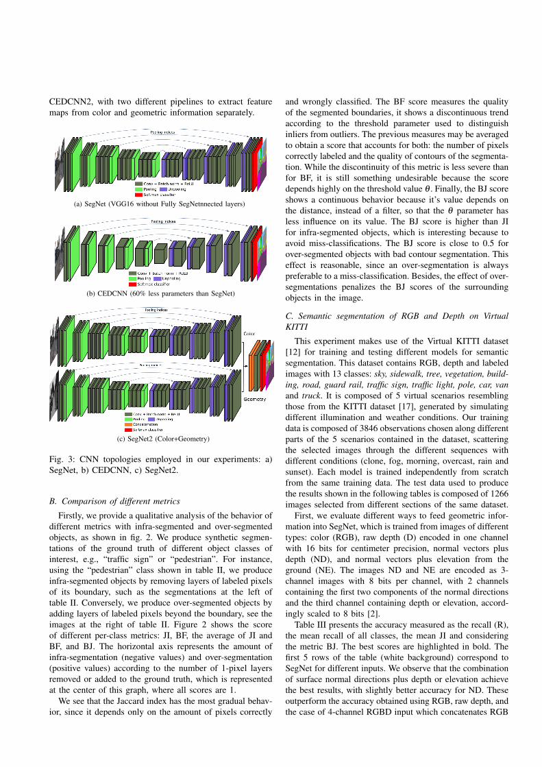
CEDCNN2, with two different pipelines to extract featuremaps from color and geometric information separately.

(a) SegNet (VGG16 without Fully SegNetnnected layers)

(b) CEDCNN (60% less parameters than SegNet)

(c) SegNet2 (Color+Geometry)

Fig. 3: CNN topologies employed in our experiments: a)SegNet, b) CEDCNN, c) SegNet2.

B. Comparison of different metrics

Firstly, we provide a qualitative analysis of the behavior ofdifferent metrics with infra-segmented and over-segmentedobjects, as shown in fig. 2. We produce synthetic segmen-tations of the ground truth of different object classes ofinterest, e.g., “traffic sign” or “pedestrian”. For instance,using the “pedestrian” class shown in table II, we produceinfra-segmented objects by removing layers of labeled pixelsof its boundary, such as the segmentations at the left oftable II. Conversely, we produce over-segmented objects byadding layers of labeled pixels beyond the boundary, see theimages at the right of table II. Figure 2 shows the scoreof different per-class metrics: JI, BF, the average of JI andBF, and BJ. The horizontal axis represents the amount ofinfra-segmentation (negative values) and over-segmentation(positive values) according to the number of 1-pixel layersremoved or added to the ground truth, which is representedat the center of this graph, where all scores are 1.

We see that the Jaccard index has the most gradual behav-ior, since it depends only on the amount of pixels correctly

and wrongly classified. The BF score measures the qualityof the segmented boundaries, it shows a discontinuous trendaccording to the threshold parameter used to distinguishinliers from outliers. The previous measures may be averagedto obtain a score that accounts for both: the number of pixelscorrectly labeled and the quality of contours of the segmenta-tion. While the discontinuity of this metric is less severe thanfor BF, it is still something undesirable because the scoredepends highly on the threshold value θ . Finally, the BJ scoreshows a continuous behavior because it’s value depends onthe distance, instead of a filter, so that the θ parameter hasless influence on its value. The BJ score is higher than JIfor infra-segmented objects, which is interesting because toavoid miss-classifications. The BJ score is close to 0.5 forover-segmented objects with bad contour segmentation. Thiseffect is reasonable, since an over-segmentation is alwayspreferable to a miss-classification. Besides, the effect of over-segmentations penalizes the BJ scores of the surroundingobjects in the image.

C. Semantic segmentation of RGB and Depth on VirtualKITTI

This experiment makes use of the Virtual KITTI dataset[12] for training and testing different models for semanticsegmentation. This dataset contains RGB, depth and labeledimages with 13 classes: sky, sidewalk, tree, vegetation, build-ing, road, guard rail, traffic sign, traffic light, pole, car, vanand truck. It is composed of 5 virtual scenarios resemblingthose from the KITTI dataset [17], generated by simulatingdifferent illumination and weather conditions. Our trainingdata is composed of 3846 observations chosen along differentparts of the 5 scenarios contained in the dataset, scatteringthe selected images through the different sequences withdifferent conditions (clone, fog, morning, overcast, rain andsunset). Each model is trained independently from scratchfrom the same training data. The test data used to producethe results shown in the following tables is composed of 1266images selected from different sections of the same dataset.

First, we evaluate different ways to feed geometric infor-mation into SegNet, which is trained from images of differenttypes: color (RGB), raw depth (D) encoded in one channelwith 16 bits for centimeter precision, normal vectors plusdepth (ND), and normal vectors plus elevation from theground (NE). The images ND and NE are encoded as 3-channel images with 8 bits per channel, with 2 channelscontaining the first two components of the normal directionsand the third channel containing depth or elevation, accord-ingly scaled to 8 bits [2].

Table III presents the accuracy measured as the recall (R),the mean recall of all classes, the mean JI and consideringthe metric BJ. The best scores are highlighted in bold. Thefirst 5 rows of the table (white background) correspond toSegNet for different inputs. We observe that the combinationof surface normal directions plus depth or elevation achievethe best results, with slightly better accuracy for ND. Theseoutperform the accuracy obtained using RGB, raw depth, andthe case of 4-channel RGBD input which concatenates RGB

with raw depth (with 8 bits for each color channel and 16 bitsfor depth) 1. Regarding the accuracy of the model SegNet2(see fig. 3c), the use of input data from RGB-ND achievesthe best results, for which all the global accuracy metricsindicate that it is the best model. Note that recall measuredon the class borders are very close to the mean recall. In fact,both measures are quite similar because computing the recallonly on class borders leverages the effect of unbalancedfrequencies of the different classes, while being more stableto the presence of low-frequency (“rare”) classes with lowerclass-wise accuracy.

TABLE III: Semantic segmentation accuracy of SegNet andSegNet2 using color and geometric information (in %).

Model \ Metric recall m. R m. JI BJSegNet (RGB) 81.7 61.9 41.2 61.7SegNet (D) 85.8 65.2 47.0 67.1SegNet (ND) 88.6 70.2 51.1 69.8SegNet (NE) 88.5 71.5 48.9 69.5SegNet (RGBD) 78.1 64.1 41.8 60.7SegNet2 (RGB-D) 88.5 71.0 49.4 70.5SegNet2 (RGB-ND) 90.3 71.8 52.9 71.7

We analyze next other network architectures like FuseNet[8], together with the network topologies introduced insection IV-A: SegNet2, CEDCNN and CEDCNN2. Table IVshows the accuracy measured with the same global statisticsof the previous table. For easier reference, this table alsoshows the results of SegNet for RGB and SegNet2 for RGB-ND in the two first rows. The results show that FuseNet,which was designed for semantic segmentation of indoor im-ages from RGB-D data, achieves a performance comparablewith SegNet. The authors of FuseNet argued in [8] that therelevant geometric features can be learned from raw depthby the CNN without the need of previous transformations.However, we observe a relevant improvement by comparingthe results of FuseNet using RGB-D vs. RGB-ND, for whichthe surface directions contribute to improve the accuracy.For this case, the images are “virtually” acquired from aforward facing camera mounted in a car. Therefore, thesurface directions have some invariants, such as the anglewith gravity, that constitute a relevant source of information.

TABLE IV: Global accuracy of different types of networksusing color and geometric information (in %).

Model \ Metric recall m. R m. JI BJSegNet (RGB) 81.7 61.9 41.2 61.7SegNet2 (RGB-ND) 88.6 70.2 51.1 69.8FuseNet (RGB-D) 85.2 65.9 45.8 64.9FuseNet (RGB-ND) 88.1 64.6 47.2 68.9CEDCNN (RGB) 88.8 72.8 48.6 70.5CEDCNN2 (RGB-D) 90.1 79.7 60.0 77.5CEDCNN2 (RGB-ND) 92.6 81.7 64.7 80.0

We remark that the different models achieve the bestsemantic segmentation depending on the class, while the best

1Note that the virtual dataset has “perfect” geometry, which explains thehigh accuracy rates using only geometric information.

model overall (according to BJ) is CEDCNN2 with RGB-ND, which has a considerable better performance segmentingclasses with lower frequencies, such as “traffic light” or“truck”, while the scores of large frequency classes like“sky”, “tree” or “road” are generally more stable across thedifferent models. This fact is depicted in fig. 4 with confusionmatrices for three different architectures. Note that if we needto choose between one of the FuseNet models, we need toconsider the metric for all classes. Having unbalanced classfrequencies has a great influence on the final score, becausemulti-resolution CNN are well suited by design to segmentlarge homogeneous classes, but they are harder to train inorder to achieve similar scores on low frequency classes,which sometimes are more important for many practicalapplications like for the case of autonomous driving.

Regarding the different accuracy metrics, we observe thatthe mean recall and the mean JI are less stable acrossthe different experiments. This occurs because the accuracyof low frequency classes have a large variability even forsimilar models, and this variability is also reflected in theirmean values. This effect is also observed in the normalizedconfusion matrices, see fig. 4, where the diagonal elementscorrespond to recall of each class, and where the JI for thei-th class is related to the values contained the i-th row andi-th column. On the other hand, BJ presents a more stablebehavior for similar models, where even little changes on itsvalue seem to be a good indicator to choose the best modelaccording to the visualization of the predicted segmentation.

V. CORRELATION OF DIFFERENT METRICS

This section measures the correlation of the differentmetrics evaluated in the previous experiment. We computethe per-image score on the segmented test sequence of Vir-tual KITTI (RGB-ND) obtained with the model CEDCNN2,and measure the correlation of the different metrics forranking the quality of each segmented image. We employthe Spearmans rank correlation (ρ), which is a nonparametricmeasure of rank correlation, defined as the Pearson correla-tion coefficient between the ranked variables. It is used hereto measure the statistical dependence between the ranking ofdifferent accuracy metrics. For a sample of size n, with the nraw scores Xi,Yi, the Spearman’s rank correlation is definedas

ρ =cov(rgX ,rgY )

σrgX σrgY

(17)

where rgX ,rgY are the ranks of the score distributions X ,Y .Since we choose integer values for the rank, the formula issimplified to

ρ = 1− 6∑ni=1(rgXi − rgYi)

2

n(n2−1)(18)

Table V shows the ranking correlations among metrics,where we can see that the BJ score is correlated to both JI andBF, showing that they capture similar information. Noticethat the correlations with BJ are higher than the correlationsamong other pairs of scores.

(a) SegNet (RGB) (b) FuseNet (RGB-D) (c) CEDCNN2 (RGB-ND)

Fig. 4: Normalized confusion matrices (in %) of semantic segmentation in the real KITTI dataset with: a) SegNet (RGB),b) FuseNet (RGB-D) and c) CEDCNN2 (RGB-ND).

TABLE V: Spearmans rank correlation of different segmen-tation scores.

metric JI BF (JI+BF)/2 BJJI - 0.48 0.59 0.63

BF - - 0.68 0.65(JI+BF)/2 - - - 0.73

VI. CONCLUSIONS

This paper addresses the problem of measuring the ac-curacy of semantic segmentation of images, which is anessential aspect when comparing different segmentation ap-proaches. The global recall, mean recall and mean JI statis-tics have been traditionally employed to evaluate differentimage segmentation results, however, these metrics are notsatisfactory enough when the classes frequencies are veryunbalanced. We present a simple and efficient strategy tocompute the recall on border regions of the different classeswhich leverages unbalanced frequencies, and is a goodindicator to measure class segmentation. Our proposed metricencodes jointly the rate of correctly labeled pixels andhow homeomorphic is the segmentation to the real objectboundaries. We also present results for several different CNNarchitectures using two state-of-the-art benchmark datasets.Though we address this problem in the context of urbanimages segmentation, our results can also be extended toother contexts, like for indoor scenarios.

The research in this paper was partly motivated by theneed of segmentation solutions with better segmentation ofcontours, for which traditional metrics were not suitable. Inour future research, we plan to study how to give moreimportance to the segmentation of such contours duringthe training phase of the CNN and on obtaining optimalCNN designs for semantic segmentation of complex dynamicoutdoor scenes.

REFERENCES

[1] R. Drouilly, P. Rives, and B. Morisset, “Semantic representation fornavigation in large-scale environments,” in Robotics and Automation(ICRA), 2015 IEEE International Conference on. IEEE, 2015, pp.1106–1111.

[2] S. Gupta, R. Girshick, P. Arbelaez, and J. Malik, “Learning richfeatures from rgb-d images for object detection and segmentation,”in European Conference on Computer Vision. Springer, 2014, pp.345–360.

[3] L.-C. Chen, G. Papandreou, I. Kokkinos, K. Murphy, and A. L. Yuille,“Semantic image segmentation with deep convolutional nets and fullyconnected crfs,” arXiv preprint arXiv:1412.7062, 2014.

[4] J. Long, E. Shelhamer, and T. Darrell, “Fully convolutional networksfor semantic segmentation,” in Proceedings of the IEEE Conferenceon Computer Vision and Pattern Recognition, 2015, pp. 3431–3440.

[5] H. Noh, S. Hong, and B. Han, “Learning deconvolution network forsemantic segmentation,” in Proceedings of the IEEE InternationalConference on Computer Vision, 2015, pp. 1520–1528.

[6] V. Badrinarayanan, A. Kendall, and R. Cipolla, “Segnet: A deepconvolutional encoder-decoder architecture for image segmentation,”arXiv preprint arXiv:1511.00561, 2015.

[7] A. Kendall, V. Badrinarayanan, and R. Cipolla, “Bayesian segnet:Model uncertainty in deep convolutional encoder-decoder architecturesfor scene understanding,” arXiv preprint arXiv:1511.02680, 2015.

[8] C. Hazirbas, L. Ma, C. Domokos, and D. Cremers, “Fusenet: In-corporating depth into semantic segmentation via fusion-based cnnarchitecture,” in Proc. ACCV, vol. 2, 2016.

[9] L. Ladicky, P. Sturgess, K. Alahari, C. Russell, and P. H. Torr,“What, where and how many? combining object detectors and crfs,”in European conference on computer vision. Springer, 2010, pp.424–437.

[10] S. Zheng, S. Jayasumana, B. Romera-Paredes, V. Vineet, Z. Su, D. Du,C. Huang, and P. H. Torr, “Conditional random fields as recurrentneural networks,” in Proceedings of the IEEE International Conferenceon Computer Vision, 2015, pp. 1529–1537.

[11] F. Liu, G. Lin, and C. Shen, “Crf learning with cnn features for imagesegmentation,” Pattern Recognition, vol. 48, no. 10, pp. 2983–2992,2015.

[12] A. Gaidon, Q. Wang, Y. Cabon, and E. Vig, “Virtual worlds asproxy for multi-object tracking analysis,” in Proceedings of the IEEEConference on Computer Vision and Pattern Recognition, 2016, pp.4340–4349.

[13] C. Couprie, C. Farabet, L. Najman, and Y. LeCun, “Indoorsemantic segmentation using depth information,” arXiv preprintarXiv:1301.3572, 2013.

[14] A. Eitel, J. T. Springenberg, L. Spinello, M. Riedmiller, and W. Bur-gard, “Multimodal deep learning for robust rgb-d object recognition,”in Intelligent Robots and Systems (IROS), 2015 IEEE/RSJ Interna-tional Conference on. IEEE, 2015, pp. 681–687.

[15] D. Eigen and R. Fergus, “Predicting depth, surface normals and se-mantic labels with a common multi-scale convolutional architecture,”in Proceedings of the IEEE International Conference on ComputerVision, 2015, pp. 2650–2658.

[16] M. Cordts, M. Omran, S. Ramos, T. Rehfeld, M. Enzweiler, R. Be-nenson, U. Franke, S. Roth, and B. Schiele, “The cityscapes datasetfor semantic urban scene understanding,” in Proceedings of the IEEEConference on Computer Vision and Pattern Recognition, 2016, pp.3213–3223.

Fig. 5: Semantic segmentation produced by the different models. The first 2 columns correspond to test images from VirtualKITTI, while and the last 2 columns correspond to images from our KITTI test. The first row shows the input RGB image,followed by depth, groundtruth labels. Rows 4th to 7th show the segmentation produced by: CEDCNN2 (RGB-D), CEDCNN(RGB), SegNet2 (RGB-D) and SegNet (RGB) respectively. The 8th row shows the border regions from the ground truth,which are used to evaluate border recall and our metric in eq. (16). The 9th row shows the border precision of CEDCNN2(RGB-D).

[17] A. Geiger, P. Lenz, C. Stiller, and R. Urtasun, “Vision meets robotics:The kitti dataset,” The International Journal of Robotics Research,vol. 32, no. 11, pp. 1231–1237, 2013.

[18] D. R. Martin, C. C. Fowlkes, and J. Malik, “Learning to detect naturalimage boundaries using local brightness, color, and texture cues,” IEEEtransactions on pattern analysis and machine intelligence, vol. 26,no. 5, pp. 530–549, 2004.

[19] G. Csurka, D. Larlus, F. Perronnin, and F. Meylan, “What is a goodevaluation measure for semantic segmentation?.” in BMVC, vol. 27,2013, p. 2013.

[20] P. Kohli, L. Ladicky, and P. H. Torr, “Robust higher order potentialsfor enforcing label consistency,” in Computer Vision and PatternRecognition, 2008. CVPR 2008. IEEE Conference on. IEEE, 2008,pp. 1–8.

[21] J. Freixenet, X. Munoz, D. Raba, J. Martı, and X. Cufı, “Yet anothersurvey on image segmentation: Region and boundary informationintegration,” Computer VisionECCV 2002, pp. 21–25, 2002.

[22] M. Sokolova and G. Lapalme, “A systematic analysis of performancemeasures for classification tasks,” Information Processing & Manage-ment, vol. 45, no. 4, pp. 427–437, 2009.

[23] C. J. Van Rijsbergen, Information Retrieval. Butterworths, 1979.[24] K. Simonyan and A. Zisserman, “Very deep convolutional networks

for large-scale image recognition,” arXiv preprint arXiv:1409.1556,2014.