a new look at the big five factor structure through ... 2010-pa-a new.pdf · ular, an important...

A New Look at the Big Five Factor Structure Through ExploratoryStructural Equation Modeling

Herbert W. MarshUniversity of Oxford

Oliver LudtkeUniversity of Tubingen, Tubingen, Germany, and Max Planck

Institute for Human Development, Berlin, Germany

Bengt MuthenUniversity of California, Los Angeles

Tihomir AsparouhovMuthen & Muthen, Los Angeles, California

Alexandre J. S. MorinUniversity of Sherbrooke

Ulrich TrautweinUniversity of Tubingen, Tubingen, Germany, and Max Planck

Institute for Human Development, Berlin, Germany

Benjamin NagengastUniversity of Oxford

NEO instruments are widely used to assess Big Five personality factors, but confirmatory factor analyses(CFAs) conducted at the item level do not support their a priori structure due, in part, to the overlyrestrictive CFA assumptions. We demonstrate that exploratory structural equation modeling (ESEM), anintegration of CFA and exploratory factor analysis (EFA), overcomes these problems with responses(N � 3,390) to the 60-item NEO–Five-Factor Inventory: (a) ESEM fits the data better and results insubstantially more differentiated (less correlated) factors than does CFA; (b) tests of gender invariancewith the 13-model ESEM taxonomy of full measurement invariance of factor loadings, factor variances–covariances, item uniquenesses, correlated uniquenesses, item intercepts, differential item functioning,and latent means show that women score higher on all NEO Big Five factors; (c) longitudinal analysessupport measurement invariance over time and the maturity principle (decreases in Neuroticism andincreases in Agreeableness, Openness, and Conscientiousness). Using ESEM, we addressed substantivelyimportant questions with broad applicability to personality research that could not be appropriatelyaddressed with the traditional approaches of either EFA or CFA.

Keywords: exploratory structural equation modeling, factorial and measurement invariance, Big Fivepersonality structure, differential item functioning

Supplemental materials: http://dx.doi.org/10.1037/a0019227.supp

Arguably, the most important advance in personality psychol-ogy in the past half century has been the emerging consensus thatindividual differences in adults’ personality characteristics can be

organized in terms of five broad trait domains: Extraversion,Agreeableness, Conscientiousness, Neuroticism, and Openness.These Big Five factors now serve as a common language in thefield, facilitating communication and collaboration. Althoughthere are several Big Five instruments (e.g., Benet-Martinez &John, 1998; Caprara & Perugini, 1994; Goldberg, 1990; Gosling,Rentfrow, & Swann, 2003; John & Srivastava, 1999; Paunonen,2003; Paunonen & Ashton, 2001; Saucier, 1998), the family ofNEO instruments—including the 60-item NEO–Five-Factor In-ventory (NEO-FFI; Costa & McCrae, 1992; McCrae & Costa,2004) considered here—appear to be the most widely used instru-ments and to have received the most attention over recent years(Boyle, 2008).

Factor analysis has been at the heart of these exciting break-throughs. Exploratory factor analyses (EFAs) have consistentlyidentified the Big Five factors, and an impressive body of empir-ical research supports their stability and predictive validity (seeMcCrae & Costa, 1997). However, confirmatory factor analyses

Herbert W. Marsh and Benjamin Nagengast, Department of Education,University of Oxford, Oxford, England; Oliver Ludtke and Ulrich Trautwein,University of Tubingen, Tubingen, Germany, and Center for EducationalResearch, Max Planck Institute for Human Development, Berlin, Germany;Bengt Muthen, Graduate School of Education and Information Studies, Uni-versity of California, Los Angeles; Tihomir Asparouhov, Muthen & Muthen,Los Angeles, California; Alexandre J. S. Morin, Department of Psychology,University of Sherbrooke, Sherbrooke, Quebec, Canada.

This research was supported in part by a grant to Herbert W. Marsh fromthe United Kingdom’s Economic and Social Research Council.

Correspondence concerning this article should be addressed to HerbertW. Marsh, Department of Education, University of Oxford, 15 NorhamGardens, Oxford OX2 6PY, United Kingdom. E-mail: [email protected]

Psychological Assessment © 2010 American Psychological Association2010, Vol. 22, No. 3, 471–491 1040-3590/10/$12.00 DOI: 10.1037/a0019227

471

(CFAs) have failed to provide clear support for the five-factormodel on the basis of standard measures such as the NEO instru-ments. For example, in a particularly relevant study comparingEFA and CFA factor structures based on NEO–Personality Inven-tory (NEO-PI) responses, Vassend and Skrondal (1997) reportedhighly discrepant findings, leading them to conclude

(i) that the original NEO-PI model as well as later EFA-based revi-sions are false or at least unsatisfactory, and (ii) that at present we donot know how the NEO-PI scales should be modeled with the aim ofobtaining a common, acceptable NEO-PI version. (p. 157)

Problematic results based on CFAs have led some researchers toquestion the appropriateness of CFA for Big Five research (seeBorkenau & Ostendorf, 1990; Church & Burke, 1994; McCrae,Zonderman, Costa, Bond, & Paunonen, 1996; Parker, Bagby, &Summerfeldt, 1993; Vassend & Skrondal, 1997). However, manyof the methodological and statistical advances in quantitative psy-chology in the last 2 decades are associated with latent-variableapproaches such as CFA and structural equation models (SEMs).Hence, failure to embrace these new and evolving methodologies(throwing the baby out with the bathwater) would have direconsequences—particularly for a field of research so fundamen-tally based on factor analysis. Indeed, assumptions of factorial andmeasurement invariance (in relation to multiple groups, time,covariates, and outcomes) that underpin nearly all Big Five studiescannot be appropriately evaluated with traditional approaches toEFA and thus have been largely ignored in Big Five EFA research.Here we outline a new approach to factor analysis—an integrationof EFA and CFA—that has the potential to resolve this dilemmaand has wide applicability to all disciplines of psychology that arebased on the measurement of latent constructs. Thus, our study isa substantive-methodological synergy (Marsh & Hau, 2007), dem-onstrating the importance of applying new and evolving method-ological approaches to substantively important issues.

Methodological Focus: Exploratory StructuralEquation Modeling (ESEM)

EFA Versus CFA

Many measurement instruments used in psychological assess-ment apparently have well-defined EFA structures but are notsupported by CFAs (Marsh et al., 2009). This concern led McCraeet al. (1996) to conclude:

In actual analyses of personality data from Borkenau and Ostendorf(1990) to Holden and Fekken (1994), structures that are known to bereliable showed poor fits when evaluated by CFA techniques. Webelieve this points to serious problems with CFA itself when used toexamine personality structure. (p. 568; also see Costa & McCrae,1992, 1995; McCrae & Costa, 1997)

Church and Burke (1994) similarly concluded on the basis of theirempirical research that

Poor fits of a priori models highlighted not only the limited specificityof personality structure theory, but also the limitations of confirmatoryfactor analysis for testing personality structure models. (p. 93)

They argued that the independent clusters model (ICM) used inCFA studies, which requires each indicator to load on only onefactor, is too restrictive for personality research, because indicatorsare likely to have secondary loadings unless researchers resort tousing a small number of near-synonyms to infer each factor.

Marsh et al. (2009) claimed that, consistent with these concerns,many ad hoc strategies used to compensate for the inappropriate-ness of CFA in psychological research more generally are dubious,counterproductive, misleading, or simply wrong. Of particularrelevance to the present investigation, the inappropriate impositionof zero factor loadings usually leads to distorted factors withpositively biased factor correlations that might lead to biasedestimates in SEMs incorporating other constructs (also see Marshet al., 2009). In a similar vein, Marsh (2007; Marsh, Hau, &Grayson, 2005) concluded that many psychological instrumentsused in applied research do not even meet minimum criteria ofacceptable fit according to current standards.

Apparently, many applied researchers persist with inappropriateICM-CFA models because they believe that EFA approaches areoutdated and that methodological advances associated with CFAsare not applicable to EFAs. Here we demonstrate how it is possibleto apply EFA rigorously in a way that allows researchers to definemore appropriately the underlying factor structure and to stillapply the advanced statistical methods typically associated withCFAs and SEMs. This is accomplished with the ESEM procedurerecently implemented in the Mplus statistical package (Version5.2, Muthen & Muthen, 2008). Within the ESEM framework, theapplied personality researcher has access to typical SEM parame-ter estimates, standard errors, goodness-of-fit statistics, and statis-tical advances normally associated with CFA and SEMs (seeAsparouhov & Muthen, 2009; Marsh et al., 2009). Here we applyESEM to NEO-FFI responses.

Tests of Factorial and Measurement Invariance

We know of no CFAs carried out at the item level—particularlyfor research based on the NEO-FFI instrument used to measure theBig Five personality factors—that provide acceptable support forthe a priori Big Five factor structure. This is remarkable, given thewidespread acceptance of the Big Five factor structure and theNEO-FFI. Hence, it is not surprising that research into the BigFive factor structure on responses to individual items continues tobe based almost entirely on EFA (for exceptions, see Benet-Martinez & John, 1998; Dolan, Oort, Stoel, & Wichterts, 2009;Gustavsson, Eriksson, Hilding, Gunnarsson, & Ostensson, 2008;also see Reise, Smith, & Furr, 2001). We suggest that this failureto apply CFA models in Big Five research is due in large part tothe inappropriateness of the typical ICM-CFA structure. Althoughidentification of the appropriate factor structure is important in itsown right, there are many other important advantages to the use ofCFA that cannot be easily incorporated into EFA and thus havebeen largely ignored in Big Five personality research. Thus, forexample, studies that use Big Five scale scores (or factor scoresbased on EFAs) are not corrected for measurement error. Althoughit is possible to correct for a simple form of measurement error(i.e., the typical correction for attenuation based on reliabilityestimates), in many applications the error structure is more com-plex (e.g., longitudinal studies as considered here), so the typicalcorrection for attenuation is not sufficient.

472 MARSH ET AL.

A particularly important application of CFA techniques is to testthe assumptions about the invariance of the Big Five factor struc-ture over multiple groups or over time (Gustavsson et al., 2008;Nye, Roberts, Saucier, & Zhou, 2008; Reise et al., 2001). Unlessthe underlying factors are measuring the same construct in thesame way and the measurements themselves are operating in thesame way (across groups or over time), mean differences and othercomparisons are likely to be invalid. Although some aspects offactor similarity can be addressed in part with EFA approaches(e.g., the similarity of the factor loadings), most cannot. In partic-ular, an important assumption in the comparison of Big Fivefactors over different groups (e.g., men and women) or over timeis the invariance of item intercepts. More specifically, it is impor-tant to ascertain that mean differences based on latent constructs(Big Five factors) are reflected in each of the individual items usedto infer the latent constructs. For example, if the apparent level ofgender differences in Extraversion varies substantially from itemto item for different items used to infer this construct, then thegender differences based on the corresponding latent construct areidiosyncratic to the particular items used to infer Extraversion.Similarly, if responses to individual Extraversion items differsystematically with age (for different respondents) or over time(for the same respondents), then findings based on comparisons ofscale scores might be invalid. In each case, these results wouldsuggest that conclusions about differences in Extraversion do notgeneralize over even the set of items used in the instrument—letalone the population of items that could have been used. Hence,conclusions about differences in Extraversion might be idiosyn-cratic to the particular set of items and not be generalizable. Fromthis perspective, it is important to evaluate the invariance ofdifferent aspects of the factor structure at the level of the individualitem. Although issues of noninvariance of item intercepts (hereaf-ter referred to as differential item functioning) are well known inevaluating the appropriateness of standardized achievement tests,these issues have been largely ignored in Big Five research (butsee Jackson et al., 2009; Nye et al., 2008; Reise et al., 2001).

Substantive Focus on Big Five Personality Factorsand the NEO-FFI

Gender Differences in Personality Traits

There is a long history of the search for gender differences inpersonality research (e.g., Feingold, 1994; Hall, 1984; Maccoby &Jacklin, 1974). Noting that Feingold (1994) had organized hisreview in part on the basis of the five broad factors and 30 facetsof the NEO-PI, Costa, Terracciano, and McCrae (2001) greatlyexpanded the research based on the 30 facets measured by theNEO-PI-R for responses from 26 countries (N � 23,031). Inter-estingly, they found that gender differences within the set of sixfacets comprising each of the Big Five factors were not entirelyconsistent. Women had consistently higher scores across six facetsrepresenting Neuroticism and Agreeableness, whereas gender dif-ferences were consistently small for Conscientiousness. However,gender differences were less consistent for Extraversion and Open-ness; for each of these Big Five factors at least two (of six) facetsfavored women and at least two favored men. Hence, the size andeven the direction of gender differences would differ depending onwhich facet (or mix of facets) was considered. Thus, even at the

facet level there is apparently differential item (facet) functioningfor some of the Big Five factors that compromises conclusionsbased on Big Five measures that are aggregated across facets.Logically, this implies that there is also likely to be differentialitem functioning at the level of individual items in relation togender differences for NEO-FFI responses considered here.

Although there is considerable study-to-study variation in ob-served gender differences that may be a function of age, nation-ality, and the particular instrument considered, there is clear sup-port for the conclusions that women tend to score higher than menin relation to Neuroticism and Agreeableness. Although less con-sistent, there is also evidence that women score higher on Consci-entiousness and Extraversion but no clear support for evidence ofgender differences in Openness. There is no evidence that menscore higher than women on any of the Big Five factors asmeasured and labeled on the NEO-FFI (although women’s higherscores on Neuroticism are sometimes summarized as lower scoreson emotional stability). Particularly relevant to the current study(based on late-adolescent responses by Germans), Schmitt, Realo,Voracek, and Allik (2008) reported that for their German sample(N � 790), women scored higher than men did on all Big Fivefactors: Neuroticism (d � 0.48), Extraversion (d � 0.12), Agree-ableness (d � 0.09), Conscientiousness (d � 0.23), and Openness(d � 0.11). Similarly, Donnellan and Lucas (2008) found that forthe late-adolescent sample (ages 16–19 years) most relevant to thepresent investigation, German women consistently scored higherthan German men did: Neuroticism (d � 0.47), Extraversion (d �0.24), Agreeableness (d � 0.31), Conscientiousness (d � 0.34),and Openness (d � 0.36).

Longitudinal Invariance: Stability and Change inPersonality Traits

The literature on personality development distinguishes severaltypes of personality change and continuity (Caspi & Shiner, 2006;Ludtke, Trautwein, & Husemann, 2009). Here we distinguishbetween correlational (rank-order), mean-level, and structural sta-bility over time.

For correlational stability, cross-sectional and longitudinal re-search (Roberts & DelVecchio, 2000; see also Fraley & Roberts,2005; Klimstra, Hale, Raaijmakers, Branje, & Meeus, 2009;Ludtke et al., 2009) shows that correlational stability increaseswith age, particularly for the middle-to-late adolescent period thatis the focus of the present investigation.

Studies of mean-level change with respect to life-span changesin Big Five traits show that most people become more dominant,agreeable, conscientious, and emotionally stable. Caspi, Roberts,and Shiner (2005) coined the term maturity principle to describethese findings of increasing psychological maturity from adoles-cence to middle age. In their meta-analysis of longitudinal studies,Roberts, Walton, and Viechtbauer (2006) also found substantialincreases in Openness. For the 18–22 age group most relevant tothe present investigation, Robins, Fraley, Roberts, and Trz-esniewski (2001) found that, over a 4-year period, Agreeableness(d � 0.44), Conscientiousness (d � 0.27), and Openness (d �0.22) increased and Neuroticism (d � –0.49) decreased. No sta-tistically significant change was found for Extraversion. In sum-mary, although results from these studies are not entirely consis-tent, there is general support for the maturity principle of increases

473NEW LOOK AT BIG FIVE FACTOR STRUCTURE

in all Big Five factors (or decreases in Neuroticism instead ofincreases in Emotional Stability) except, perhaps, for Extraversion.

Structural stability assesses the extent to which the same factorsare being assessed in different groups or over time. At least somelevel of structural invariance is a prerequisite for assessing eithermean differences between groups or stability over time. If thenature of the factors changes so that factors are qualitativelydifferent, then interpretations of stability over time are question-able. It is most appropriate to evaluate factorial and measurementinvariance on the basis of responses to individual items. However,personality researchers have been remarkably unsuccessful in ob-taining acceptable levels of goodness of fit for the a priori Big Fivefactor CFA structure when analysis of the structure is based onresponses to individual items in studies of the NEO-FFI instrumentconsidered here. Indeed, this might be considered the major lim-itation in Big Five personality research, particularly in relation totesting assumptions underpinning the valid assessment of stabilityover time as well as the valid comparison of latent means acrossgroups. For this reason some studies have sought to formally test fullmeasurement invariance based on mean responses averaged acrossdifferent items, facet scores (e.g., Gignac, 2009; McCrae et al., 1996;Saucier, 1998; Small, Hertzog, Hultsch, & Dixon, 2003), parcelscores (Allemand, Zimprich, & Hendriks, 2008; Allemand, Zimprich,& Hertzog, 2007; Ludtke et al., 2009; Marsh, Trautwein, Ludtke,Koller, & Baumert, 2006), or scale scores (e.g., Mroczek & Spiro,2003). Although these analyses are potentially useful, they haveimportant limitations when conducted without prior verification ofmeasurement invariance at the item level—an assumption underlyingtests of mean differences (over time or across groups) and differentialitem functioning that could compromise the validity of interpretationsbased on analyses of aggregated scores (see later discussion forfurther elaboration). In the present investigation, we address theseconcerns, introducing a new ESEM approach that integrates the logicof the EFA approach typically used in Big Five personality researchand the CFA approach widely argued to be inappropriate to Big Fiveresearch.

The Present Investigation:A Substantive-Methodological Synergy

Our study is a substantive-methodological synergy, demonstrat-ing the power and flexibility of ESEM methods that integrate CFAand EFA (on the basis of the Mplus statistical package; Muthen &Muthen, 2008) to address substantively important issues about theBig Five factor structure on the basis of responses to the 60-itemNEO-FFI instrument. We begin by comparing CFA and ESEMapproaches, testing the assumption that ESEM models fit betterthan corresponding CFA models. For both CFA and ESEM mod-els, we include both freely estimated uniquenesses (reflecting acombination of measurement-error-specific variances) and a prioricorrelated uniquenesses (CUs; covariances between the specificvariance components associated with two different items from thesame Big Five facet). Big Five theory posits that the Big Fivefactors should be reasonably orthogonal, but constraining all (non-target) cross-loadings to be zero in the ICM-CFA model is positedto systematically inflate and bias estimates of the factor correla-tions. Hence, support for the prediction that Big Five factors arereasonably orthogonal is hypothesized to be stronger in ESEMmodels than in CFA models.

We then extend ESEM to test a 13-model taxonomy of mea-surement invariance, testing invariance of factor loadings, factorvariances–covariances, item uniquenesses, CUs, item intercepts,and latent means—with a specific focus on gender differences inthe latent means of the Big Five factors. Of particular interest aretests of the invariance of item intercepts that are an implicitassumption in the comparison of latent (or manifest) group meansbut are largely ignored in previous Big Five research (but seeJackson et al., 2009; Nye et al., 2008; Reise et al., 2001). Weexpect, on the basis of previous research, systematic differences,mostly reflecting higher means for women (particularly for thelate-adolescent German sample considered here). We also predictthat, consistent with previous research, there is differential itemfunctioning in NEO-FFI responses (noninvariance of item inter-cepts) that would compromise the interpretation of latent meancomparisons, but we explore alternatives to circumvent this prob-lem.

Finally, we apply ESEM to test–retest data, testing a set ofmodels of measurement invariance over time with the inclusion ofCUs relating responses to the same item on multiple occasions.Although these (within-group) tests of longitudinal invariancelargely parallel those based on (between-group) tests over gender,the substantive implications are quite different. Indeed, given thatparticipants are tested in their final year of high school at Time 1(T1) and are tested 2 years after graduation at Time 2 (T2), it isreasonable that there might be systematic changes in Big Fivelatent means. We expect to see, based on the maturity principle,decreases in Neuroticism and increases in Agreeableness, Open-ness, and Conscientiousness.

Previous research has suggested a problem with the evaluationof stability over time for NEO-FFI responses that is especiallyrelevant to the present investigation. NEO-FFI responses consis-tently have high levels of short-term test–retest stability (.86–.90;McCrae & Costa, 2004; Robins et al., 2001) and internal consis-tency (.68–.86; Costa & McCrae, 1992). However, this researchsuggests problems associated with a complex error structure in thattest–retest correlations are larger than internal consistency mea-sures of reliability. In particular, test–retest correlations would begreater than 1.0 if corrected for (internal consistency) unreliability.This suggests that observed test–retest correlations are more pos-itively biased by CUs associated with specific variances of thesame items administered on different occasions than negativelybiased by the failure to control for measurement error in thefactors. Traditional EFA approaches are unable to appropriatelydistinguish between measurement error on each occasion, CUsover time, and true stability of latent traits over time, but theseissues can be addressed by ESEM, as demonstrated in the presentinvestigation.

Method

Participants

The data come from a large, ongoing German study (Transfor-mation of the Secondary School System and Academic Careers[TOSCA]; see Koller, Watermann, Trautwein, & Ludtke, 2004;also see Ludtke et al., 2009; Marsh, Trautwein, et al., 2006). Arandom sample of 149 upper secondary schools in a single Germanstate was selected to be representative of the traditional and voca-

474 MARSH ET AL.

tional gymnasium school types attended by the college-boundstudent population. At T1, the students (N � 3,390; 45% men,55% women) were in their final year of upper secondary schooling(M age � 19.51, SD � 0.77). Two trained research assistantsadministered materials in each school, and students participatedvoluntarily, without any financial incentive. At T1, all studentswere asked to provide written consent to be contacted again laterfor a second wave of data collection. At T2, 2 years after gradu-ation from high school, participants completed an extensive ques-tionnaire taking about 2 hr in exchange for a financial reward of 10euros (US$13).

For evaluation of longitudinal stability, our analyses are re-stricted to the responses by the 1,570 (39% men, 61% women)students who completed the NEO-FFI at both T1 and T2. To testfor attrition effects, we compared continuers, who participated atboth time points, to dropouts, who participated in only the firstwave. Continuers had slightly lower grade point averages (M �2.3 vs. 2.5) and were more likely to be female. Selectivity effectsexceeding d � 0.10 were found for two of the Big Five scalescores; continuers had higher Conscientiousness and Agreeable-ness scores. Although dropouts and continuers differed statisticallysignificantly in some domains, the magnitude of these differenceswas small and indicative of only small selectivity effects. We alsocompare, as part of the analysis, factor structures based on allstudents at T1 as well as those who completed instruments at bothT1 and T2.

Measures: Big Five Dimensions

The 60-item NEO-FFI (Costa & McCrae, 1992) provides a shortmeasure of the Big Five personality factors (Costa & McCrae,1989). For each factor, McCrae and Costa (1989) selected 12 itemsfrom the 180 items of the longer NEO-PI (and the full 240-itemNEO-PI-R), based primarily on correlations between each NEO-PIitem and factor scores (McCrae & Costa, 1989). We measured theBig Five factors using the German version (Borkenau & Osten-dorf, 1993) of the NEO-FFI, whose responses have high reliability,validity, and comparability with responses to the original English-language version (e.g., Borkenau & Ostendorf, 1993). In our study,items were rated on a 4-point scale ranging from 1 (stronglydisagree) to 4 (strongly agree). Psychometric analyses of the4-point response format show that this format has some advantagesover a 5-point scale (Ludtke, Trautwein, Nagy, & Koller, 2004).Coefficient alpha reliabilities at T1 and T2, respectively, were .78and .80 (Extraversion), .72 and .73 (Agreeableness), .83 and .84(Conscientiousness), .83 and .87 (Neuroticism), and .73 and .74(Openness). Hence, consistent with previous research (e.g., Church& Burke, 1994; McCrae et al., 1996), there are small increases inreliability with increased age during this late-adolescent period.

Statistical Analyses

Analyses were conducted with Mplus (Version 5.2; Muthen &Muthen, 2008). Preliminary analyses consisted of a traditionalCFA based on the Mplus robust maximum likelihood estimator(MLR), with standard errors and tests of fit that are robust inrelation to nonnormality and nonindependence of observations(Muthen & Muthen, 2008). The main focus is on the application ofESEM to responses to the 60-item NEO Big Five personality

instrument. The ESEM approach differs from the typical CFAapproach in that all factor loadings are estimated, subject to con-straints so that the model can be identified (for further details ofthe ESEM approach and identification issues, see technical appen-dix, Appendix 1 in the online supplemental materials; also seeAsparouhov & Muthen, 2009). Here we used an oblique geominrotation (the default in the Mplus) with an epsilon value of .5 andthe MLR estimation. A critical advantage of the ESEM approachis the ability to test full measurement invariance for an EFAsolution in relation to multiple groups or occasions.

Factorial and measurement invariance. Marsh et al. (2009)proposed a 13-model taxonomy of invariance tests that integratedfactor analysis (e.g., Joreskog & Sörbom, 1988; Marsh, 1994,2007) and measurement invariance (e.g., Meredith, 1964, 1993;Meredith & Teresi, 2006) traditions to testing invariance overmultiple groups or occasions. Following the measurement invari-ance tradition, we use terminology proposed by Meredith (1964,1993) that has achieved broad acceptance. Although tests of in-variance are frequently based on covariance matrices emergingfrom the factor analysis tradition, tests of full measurement invari-ance begin with raw data (or mean augmented covariance matri-ces) and should be done at the item level to evaluate item func-tioning.

In the Meredith (1964, 1993) tradition, the sequence of invari-ance testing generally begins with a model with no invariance ofany parameter estimates (i.e., all parameters are freely estimated)such that only similarity of the overall pattern of parameters isevaluated (configural invariance). Technically, this model mightnot be an invariance model in that it does not require any estimatedparameters to be the same. However, it does provide both a test ofthe ability of the a priori model to fit the data in each group (oroccasion) without invariance constraints and a baseline for com-paring other models that do impose equality constraints on theparameter estimates across groups or over time. Configural invari-ance models are followed by tests of weak measurement invari-ance that are satisfied if factor loadings are invariant over groupsor occasions, although Byrne, Shavelson, and Muthen (1989) alsoargued for the usefulness of a less demanding test of partialinvariance in which some parameter estimates are not constrainedto be invariant. Strong measurement invariance is satisfied if theindicator means (i.e., the intercepts of responses to individualitems) and factor loadings are invariant over groups. If factorloadings and item intercepts are invariant over groups, thenchanges in the latent factor means can reasonably be interpreted aschanges in the latent constructs. Strict measurement invariance issatisfied if factor loadings, item intercepts, and item uniquenessesare all invariant across groups or over time. Strict measurementinvariance is required in order to compare Big Five (manifest)scale scores (or factor scores) over time or across different groups.As comparisons based on latent constructs are corrected for mea-surement error, they require only strong measurement invariance.

The taxonomy of 13 partially nested models (Marsh et al., 2009)expand this measurement invariance tradition; models vary fromthe least restrictive model of configural invariance with no invari-ance constraints to a model of complete invariance that posits strictinvariance as well as the invariance of the latent means and of thefactor variance–covariance matrix (see Table 1; for a more ex-tended discussion of these issues, see also Marsh et al., 2009). Allmodels except the configural invariance model (Model 1) assume


the invariance of factor loadings, but it is possible to test, forexample, the invariance of indicator uniquenesses with or withoutthe invariance of item intercepts. However, models with freelyestimated indicator intercepts and freely estimated latent means arenot identified. So in models with freely estimated intercepts, thelatent means are fixed to be zero. Then, when the intercepts areconstrained to equality across groups (or occasions), the latentmeans are constrained to be zero in one group (or occasion) andfreely estimated in the second group (or occasion). In this manner,the latent means in the second group (or occasion) and theirstatistical significance reflect the differences between the twogroups (or occasions).

Here we demonstrate the application of tests of measurementinvariance over gender and across time on the basis of our taxon-omy of invariance tests (see Table 1). Such tests have typicallyused SEM/CFA. Related multiple-group methods have been pro-posed for EFA (e.g., Cliff, 1966; Meredith, 1964), but they mainlyfocus on the similarity of factor patterns rather than formal tests ofinvariance (but also see Dolan et al., 2009). However, the ESEMmodel can be extended to multiple groups or longitudinal analysessuch that the ESEM solution is estimated separately for each groupor occasion and parameters can be constrained to be invariantacross groups or over time (Marsh et al., 2009; also see technicalappendix, Appendix 1 in the supplemental materials).

CUs. In general, the use of ex post facto CUs should beavoided (e.g., Marsh, 2007), but there are some circumstances inwhich a priori CUs should be included. When the same items areused on multiple occasions, there are likely to be correlationsbetween the unique components of the same item administered onthe different occasions that cannot be explained in terms of cor-relations between the factors. Indeed, Marsh and Hau (1996;Marsh, 2007), Joreskog (1979), and others have argued that thefailure to include these CUs is likely to systematically bias param-eter estimates such that test–retest correlations among matchinglatent factors are systematically inflated, which can then system-atically bias other parameter estimates (especially in SEMs). In theextreme, test–retest correlations might be so substantially inflatedthat the failure to include appropriate CUs can result in impropersolutions such as a nonpositive definite factor variance–covariancematrix or estimated test–retest correlations that are greater than 1.0(e.g., Marsh, Martin, & Debus, 2001; Marsh, Martin, & Hau,2006). Previous research showed that short-term test–retest corre-lations for NEO-FFI factors are systematically larger than internalconsistency estimates of reliability so that disattenuated test–retestcorrelations would be greater than 1.0 (see earlier discussion). Thissuggests that there are likely to be substantial CUs test–retest dataconsidered here. For this reason, Marsh and Hau argued that CUsrelating responses to the same items on different occasions shouldalways be included in the a priori model, but it is easy to evaluatethe extent to which the exclusion of these a priori CUs affects thefit of the model and the nature of parameter estimates (particularlytest–retest stability coefficients) by constraining them to be zero.Importantly, it is difficult to either test or correct complex struc-tures of measurement error with EFAs and scale scores typicallyused in Big Five research.

As described in more detail by McCrae and Costa (2004), in theNEO-PI-R (with 240 items), each of the Big Five factors wasrepresented by six facets, and each facet was represented bymultiple items. However, in the construction of the (short)NEO-FFI, items were selected to best represent each of the BigFive factors without reference to the facets. More specifically,each Big Five factor was represented by a factor score (based onan EFA with varimax rotation), and items were selected that weremost highly correlated with this factor score. Hence, some facetsare overrepresented (relative to the design of the full NEO-PI-R),whereas other facets are represented by a single item or notrepresented at all. We posited that items that came from the samefacet of a specific Big Five factor would have higher correlationsthan would items that came from different facets of the same BigFive factor—beyond correlations that could be explained in termsof the common Big Five factor that they represented. Here wemodeled these potentially inflated correlations due to facets asCUs relating each pair of items from the same facet. Based on themapping of NEO-FFI items onto the NEO-PI-R facets (R. McCrae,personal communication, December 1, 2008; also see Appendix 2of the supplemental materials), this resulted in an a priori set of 57CUs inherent to the design of the NEO-FFI. Although we arguethat this set of a priori CUs should be included in all factoranalyses of NEO-FFI responses, we systematically evaluate mod-els with and without these CUs as well as the invariance of theseCUs over multiple (gender) groups and over time.

Goodness of fit. CFA/SEM research typically focuses on theability of a priori models to fit the data as summarized by sample

Table 1Taxonomy of Invariance Tests for Evaluating MeasurementInvariance of Big Five Responses Across Multiple Groups orOver Multiple Occasions

Model Parameters constrained to be invariant

1 None (configural invariance)2 FL [1] (weak factorial/measurement invariance)3 FL, Uniq [1, 2]4 FL, FVCV [1, 2]5 FL, Inter [1, 2] (strong factorial/measurement invariance)6 FL, Uniq, FVCV [1–4]7 FL, Uniq, Inter [1–3, 5] (strict factorial/measurement

invariance)8 FL, FVCV, Inter [1, 2, 4, 5]9 FL, Uniq, FVCV, Inter [1–8]

10 FL, Inter, LFMn [1, 2, 5] (latent mean invariance)11 FL, Uniq, Inter, LFMn [1–3, 5, 7, 10] (manifest mean

invariance)12 FL, FVCV, Inter, LFMn [1, 2, 4–6, 8, 10]13 FL, Uniq, FVCV, Inter, LFMn [1–12] (complete factorial

invariance)

Note. Models with freely estimated LFMn constrain intercepts to beinvariant across groups, whereas models in which intercepts are free implythat mean differences are a function of intercept differences. Values inbrackets represent nesting relations in which the estimated parameters ofthe less general model are a subset of the parameters estimated in the moregeneral model under which it is nested. All models are nested under Model1 (with no invariance constraints), whereas Model 13 (complete invari-ance) is nested under all other models. FL � factor loadings; Uniq � itemuniquenesses; FVCV � factor variances–covariances; Inter � item inter-cepts; LFMn � latent factor means. Parts of this table were adapted from“Exploratory Structural Equation Modeling, Integrating CFA and EFA:Application to Students’ Evaluations of University Teaching,” by H. W.Marsh, B. Muthen, T. Asparouhov, O. Ludtke, A. Robitzsch, A. J. S.Morin, and U. Trautwein, 2009, Structural Equation Modeling, 16, p. 443,Table 1. Copyright 2009 by Taylor & Francis.

476 MARSH ET AL.

size independent indices of fit (e.g., Marsh, 2007; Marsh, Balla, &Hau, 1996; Marsh, Balla, & McDonald, 1988; Marsh et al., 2005).Here we consider the root-mean-square error of approximation(RMSEA), the Tucker–Lewis index (TLI), and the comparative fitindex (CFI), as operationalized in Mplus in association with theMLR estimator (Muthen & Muthen, 2008). We also considered therobust chi-square test statistic and evaluation of parameter esti-mates. For both the TLI and CFI, values greater than .90 and .95,respectively, typically reflect acceptable and excellent fit to thedata. For the RMSEA, values less than .05 and .08 reflect a closefit and a reasonable fit to the data, respectively (Marsh, Hau, &Wen, 2004). However, we emphasize that these cutoff valuesconstitute only rough guidelines; there is considerable evidencethat realistically large factor structures (e.g., instruments with atleast 50 items and at least five factors) are typically unable tosatisfy even the minimally acceptable standards of fit (Marsh,2007; Marsh et al., 2005; also see Marsh, Hau, Balla, & Grayson,1998). However, because there are few applications of ESEM—and none that fully evaluate the appropriateness of the traditionalCFA indices of fit—it is unclear how relevant these CFA indicesand proposed cutoff values are for ESEM studies (Marsh et al.,2009).

In CFA studies it is typically more useful to compare the relativefit of a taxonomy of nested (or partially nested) models designeda priori to evaluate particular aspects of interest than to comparethat of single models (Marsh, 2007; Marsh et al., 2009). Any twomodels are nested so long as the set of parameters estimated in themore restrictive model is a subset of the parameters estimated inthe less restrictive model. This comparison can be based on achi-square difference test, but this test suffers the same problemsas the chi-square test used to test goodness of fit that led to thedevelopment of fit indices (see Marsh et al., 1998). For this reason,researchers have posited a variety of ad hoc guidelines to evaluatewhen differences in fit are sufficiently large to reject a moreparsimonious model (i.e., the more highly constrained model withfewer estimated parameters) in favor of a more complex model. Ithas been suggested that support for the more parsimonious modelrequires a change in CFI of less than .01 (Chen, 2007; Cheung &Rensvold, 2001) or a change in RMSEA of less than .015 (Chen,2007). Marsh (2007) noted that some indices (e.g., TLI andRMSEA) incorporate a penalty for parsimony so that the moreparsimonious model can fit the data better than a less parsimoniousmodel can (i.e., the gain in parsimony is greater than the loss infit). Hence, a more conservative guideline is that the more parsi-

monious model is supported if the TLI or RMSEA is as good as orbetter than that for the more complex model. Nevertheless, allthese proposals should be considered as rough guidelines or rulesof thumb.

Especially in relation to the taxonomy of invariance tests, sup-port for the invariance of a set of parameters should be based inpart on the similarity of parameters in models that do not imposeinvariance constraints as well as on the goodness of fit in modelsthat do. Here we focus on both the similarity of the patterns ofparameters and the levels of the parameter estimates. For example,here we evaluate the similarity of factor loadings on the basis ofvarious CFA and ESEM models—whether the same item has arelatively high or low factor loading across different groups (oroccasions)—with a profile similarity index (PSI). To compute thePSI, we simply construct a column that contains all the factorloadings for one group and a second column of correspondingfactor loadings for the second group and then correlate the valuesfrom the two columns. Hence the PSI is merely the correlationbetween the two sets of factor loadings. To evaluate levels of theparameter estimates, we compare descriptive statistics for the setof coefficients in each group. Ultimately, however, an evaluationof goodness of fit must be based upon a subjective integration ofmany sources of information, including fit indices, a detailedevaluation of parameter estimates in relation to a priori hypotheses,previous research, and common sense.

Results

Big Five Factor Structure: ESEM Versus CFA

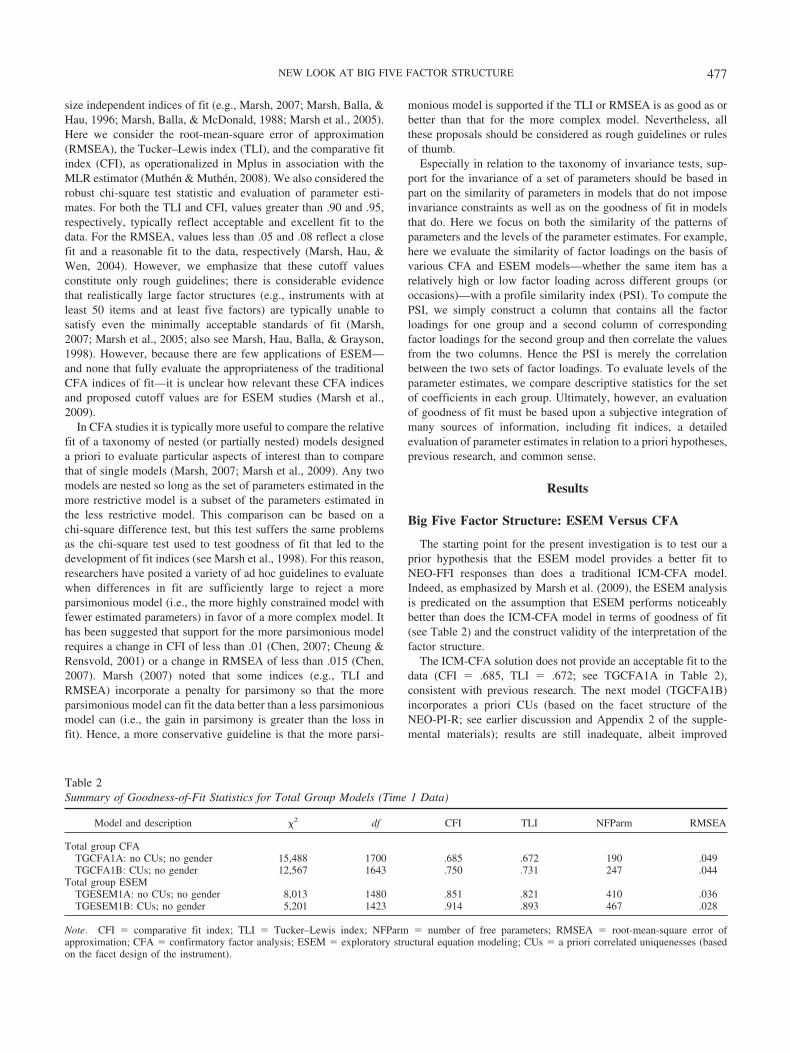
The starting point for the present investigation is to test our aprior hypothesis that the ESEM model provides a better fit toNEO-FFI responses than does a traditional ICM-CFA model.Indeed, as emphasized by Marsh et al. (2009), the ESEM analysisis predicated on the assumption that ESEM performs noticeablybetter than does the ICM-CFA model in terms of goodness of fit(see Table 2) and the construct validity of the interpretation of thefactor structure.

The ICM-CFA solution does not provide an acceptable fit to thedata (CFI � .685, TLI � .672; see TGCFA1A in Table 2),consistent with previous research. The next model (TGCFA1B)incorporates a priori CUs (based on the facet structure of theNEO-PI-R; see earlier discussion and Appendix 2 of the supple-mental materials); results are still inadequate, albeit improved

Table 2Summary of Goodness-of-Fit Statistics for Total Group Models (Time 1 Data)

Model and description �2 df CFI TLI NFParm RMSEA

Total group CFATGCFA1A: no CUs; no gender 15,488 1700 .685 .672 190 .049TGCFA1B: CUs; no gender 12,567 1643 .750 .731 247 .044

Total group ESEMTGESEM1A: no CUs; no gender 8,013 1480 .851 .821 410 .036TGESEM1B: CUs; no gender 5,201 1423 .914 .893 467 .028

Note. CFI � comparative fit index; TLI � Tucker–Lewis index; NFParm � number of free parameters; RMSEA � root-mean-square error ofapproximation; CFA � confirmatory factor analysis; ESEM � exploratory structural equation modeling; CUs � a priori correlated uniquenesses (basedon the facet design of the instrument).


(CFI � .750, TLI � .731). The corresponding ESEM solutions fitthe data much better. Although the fit of the total group with no apriori CUs is still not acceptable (TGESEM1A: CFI � .851,TLI � .821; see Table 2), the inclusion of CUs results in amarginally acceptable fit to the data (TGESEM1B: CFI � .914,TLI � .893, RMSEA � .028).

It is also instructive to compare parameter estimates based onthe ICM-CFA and ESEM solutions (see Appendix 3 of the sup-plemental materials). In both types of models, the factor loadingstend to be modest, with few factor loadings greater than .70 andsome factor loadings less than .30. Although CFA factor loadings(Mdn � .47) are slightly higher than those for the ESEM model(Mdn � .46), the differences are typically small and the pattern offactor loadings is similar for the CFA and ESEM solutions. Toquantify this subjective evaluation, we computed a PSI in whichthe vector of 60 CFA factor loadings was related to the corre-sponding vector of 60 EFA target loadings. The PSI (r � .87)demonstrated that ESEM and CFA factor loadings were highlyrelated. Consistent with McCrae and Costa (2004), the 14 itemsthat they noted as potentially weak also had lower factor loadingsthan the remaining 56 items did for both ICM-CFA (M � .38 vs..49, respectively) and ESEM (M � .32 vs. .48, respectively)solutions. Although a few of these 14 items performed well here,we note that these same items also did well in the original McCraeand Costa study. Importantly, almost all 60 items load morepositively on the ESEM factor that each was designed to measureand less positively on all other factors.

A detailed evaluation of the factor correlations among the BigFive factors demonstrates a critical advantage of the ESEM ap-proach over the ICM-CFA approach. Although patterns of corre-lations are similar, the CFA factor correlations (–.502 to �.400;Mdn absolute value � .197) tend to be systematically larger thanthe ESEM factor correlations (–.205 to �.140; Mdn absolutevalue � .064). Thus, for example, the negative correlation betweenNeuroticism and Extraversion is –.502 on the basis of the CFAsolution but only –.205 for the ESEM solution. Similarly, thecorrelation between Extraversion and Conscientiousness is �.400for the CFA results but only �.104 for the ESEM results. In thisrespect, the ESEM solution is more consistent with a priori pre-dictions that the Big Five personality factors are reasonably or-thogonal.

Clearly the ESEM solution is superior to the CFA solution, interms of both fit and distinctiveness of the factors that are consis-tent with Big Five theory. The comparison of results from thesetwo models provides the initial and most important test for theappropriateness of the ESEM model—at least relative to the CFAmodel. It is also important to emphasize that the goodness of fit forthe ESEM model is apparently far better than what has ever beenachieved in previous research with the NEO-FFI on the basis offactor analyses conducted at the item level.

Invariance Over Gender

How stable is the NEO-FFI factor structure over gender? Are theresystematic gender differences in latent means, and are the underlyingassumptions that are needed to justify interpretations of these resultsmet? To address these questions, we applied our taxonomy of 13ESEM models (see Table 1). The basic strategy is to apply the set of13 models designed to test different levels of factorial and measure-

ment invariance, ranging from the least demanding model, whichimposes no invariance constraints (configural invariance), to the mostdemanding model, which posits complete gender invariance in rela-tion to the Big Five factor structure, latent means, and item intercepts.However, application of this taxonomy of models is complicated bytwo features that are partially idiosyncratic to this application: the apriori CUs and tests of partial invariance of item intercepts (Byrne etal., 1989). The results already presented on the basis of the totalsample indicate that a priori CUs are necessary to achieve even aminimally acceptable fit to the data. However, it is also important todetermine the extent to which these a priori CUs are invariant overgender and how these influence the behavior of the various models.

For all 13 models we begin by evaluating the 57 a priori CUs.Hence, we first test models with no CUs (e.g., MG1 in Table 3corresponds to the first model in the invariance taxonomy in Table1). We then test two additional variations: one in which the a prioriCUs are allowed to vary for men and women (submodels labeledA in the Description column of Table 3, as in MG1A) and anotherin which the CUs are constrained to be invariant over responses bymen and women (submodels labeled B in Table 3, as in MG1B).Hence, within this set of three submodels there is a systematicnesting to evaluate the a priori CUs and their invariance overgender in relation to each of the 13 invariance models described inTable 1.

For the models that posit gender differences in latent means forthe Big Five factors, we also test several models to evaluate partialinvariance. Submodels labeled C posit partial invariance (i.e., itemintercepts identified in preliminary analyses are freely estimatedand not constrained to be invariant over gender—see subsequentdiscussion) but with no CUs. In submodels labeled D the set of57 a priori CUs is added, and in submodels labeled E these a prioriCUs are constrained to be equal over gender. Hence, within this setof five submodels there is a systematic nesting that allows evalu-ation of the CUs and their invariance over gender, partial invari-ance, and combinations of these constraints.

Model MG1 (see Table 3), with no invariance constraints, doesnot provide an acceptable fit to the data (TLI � .823, CFI � .852).Indeed, these fit statistics are approximately the same as thosebased on the total group ESEM model (see TGESEM in Table 2)with twice the degrees of freedom (2960 vs. 1480) and twice thenumber of estimated parameters (820 vs. 410). However, consis-tent with earlier results, the inclusion of the set of a priori CUssubstantially improves the fit to a marginally acceptable level(TLI � .891, CFI � .912; see MG1A in Table 3). Importantly,constraining these a priori CUs to be invariant over gender (seeMG1B in Table 3) resulted in almost no change in fit. For fitindices that control for parsimony, the fit is essentially unchangedor slightly better for MG1B than for MG1A, respectively (.891 to.892 for TLI; .028 to .028 for RMSEA). For the CFI that ismonotonic with parsimony, the change (.912 to .911) is clearly lessthan the .01 value typically used to support invariance constraints.These results are substantively important, demonstrating that thesizes of the 57 a priori CUs are reasonably invariant over gender.For each of the 13 models used to test the factorial invariance ofthe full mean structure (see Table 1), the inclusion of this set of apriori CUs substantially improves the goodness of fit to a similardegree. Furthermore, for each of these tests comparing freelyestimated CUs and constraining CUs to be invariant over gender,there is support for the invariance of the CUs. The consistency of

478 MARSH ET AL.

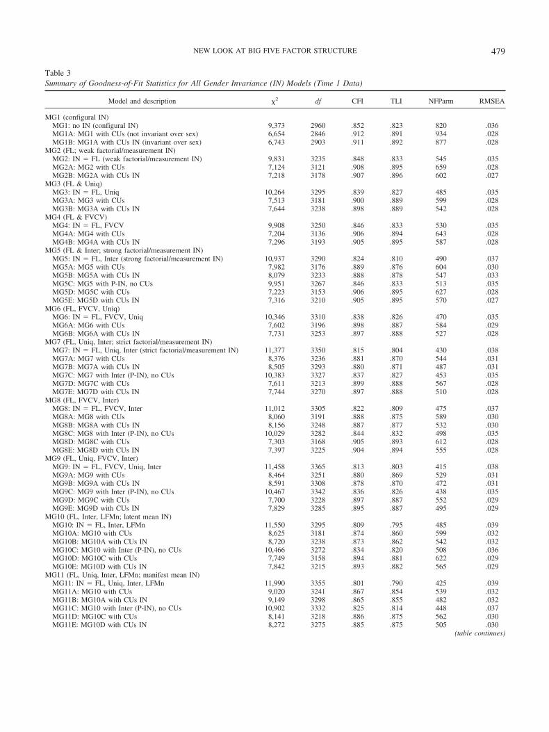
Table 3Summary of Goodness-of-Fit Statistics for All Gender Invariance (IN) Models (Time 1 Data)


MG1 (configural IN)MG1: no IN (configural IN) 9,373 2960 .852 .823 820 .036MG1A: MG1 with CUs (not invariant over sex) 6,654 2846 .912 .891 934 .028MG1B: MG1A with CUs IN (invariant over sex) 6,743 2903 .911 .892 877 .028

MG2 (FL; weak factorial/measurement IN)MG2: IN � FL (weak factorial/measurement IN) 9,831 3235 .848 .833 545 .035MG2A: MG2 with CUs 7,124 3121 .908 .895 659 .028MG2B: MG2A with CUs IN 7,218 3178 .907 .896 602 .027

MG3 (FL & Uniq)MG3: IN � FL, Uniq 10,264 3295 .839 .827 485 .035MG3A: MG3 with CUs 7,513 3181 .900 .889 599 .028MG3B: MG3A with CUs IN 7,644 3238 .898 .889 542 .028

MG4 (FL & FVCV)MG4: IN � FL, FVCV 9,908 3250 .846 .833 530 .035MG4A: MG4 with CUs 7,204 3136 .906 .894 643 .028MG4B: MG4A with CUs IN 7,296 3193 .905 .895 587 .028

MG5 (FL & Inter; strong factorial/measurement IN)MG5: IN � FL, Inter (strong factorial/measurement IN) 10,937 3290 .824 .810 490 .037MG5A: MG5 with CUs 7,982 3176 .889 .876 604 .030MG5B: MG5A with CUs IN 8,079 3233 .888 .878 547 .033MG5C: MG5 with P-IN, no CUs 9,951 3267 .846 .833 513 .035MG5D: MG5C with CUs 7,223 3153 .906 .895 627 .028MG5E: MG5D with CUs IN 7,316 3210 .905 .895 570 .027

MG6 (FL, FVCV, Uniq)MG6: IN � FL, FVCV, Uniq 10,346 3310 .838 .826 470 .035MG6A: MG6 with CUs 7,602 3196 .898 .887 584 .029MG6B: MG6A with CUs IN 7,731 3253 .897 .888 527 .028

MG7 (FL, Uniq, Inter; strict factorial/measurement IN)MG7: IN � FL, Uniq, Inter (strict factorial/measurement IN) 11,377 3350 .815 .804 430 .038MG7A: MG7 with CUs 8,376 3236 .881 .870 544 .031MG7B: MG7A with CUs IN 8,505 3293 .880 .871 487 .031MG7C: MG7 with Inter (P-IN), no CUs 10,383 3327 .837 .827 453 .035MG7D: MG7C with CUs 7,611 3213 .899 .888 567 .028MG7E: MG7D with CUs IN 7,744 3270 .897 .888 510 .028

MG8 (FL, FVCV, Inter)MG8: IN � FL, FVCV, Inter 11,012 3305 .822 .809 475 .037MG8A: MG8 with CUs 8,060 3191 .888 .875 589 .030MG8B: MG8A with CUs IN 8,156 3248 .887 .877 532 .030MG8C: MG8 with Inter (P-IN), no CUs 10,029 3282 .844 .832 498 .035MG8D: MG8C with CUs 7,303 3168 .905 .893 612 .028MG8E: MG8D with CUs IN 7,397 3225 .904 .894 555 .028

MG9 (FL, Uniq, FVCV, Inter)MG9: IN � FL, FVCV, Uniq, Inter 11,458 3365 .813 .803 415 .038MG9A: MG9 with CUs 8,464 3251 .880 .869 529 .031MG9B: MG9A with CUs IN 8,591 3308 .878 .870 472 .031MG9C: MG9 with Inter (P-IN), no CUs 10,467 3342 .836 .826 438 .035MG9D: MG9C with CUs 7,700 3228 .897 .887 552 .029MG9E: MG9D with CUs IN 7,829 3285 .895 .887 495 .029

MG10 (FL, Inter, LFMn; latent mean IN)MG10: IN � FL, Inter, LFMn 11,550 3295 .809 .795 485 .039MG10A: MG10 with CUs 8,625 3181 .874 .860 599 .032MG10B: MG10A with CUs IN 8,720 3238 .873 .862 542 .032MG10C: MG10 with Inter (P-IN), no CUs 10,466 3272 .834 .820 508 .036MG10D: MG10C with CUs 7,749 3158 .894 .881 622 .029MG10E: MG10D with CUs IN 7,842 3215 .893 .882 565 .029

MG11 (FL, Uniq, Inter, LFMn; manifest mean IN)MG11: IN � FL, Uniq, Inter, LFMn 11,990 3355 .801 .790 425 .039MG11A: MG10 with CUs 9,020 3241 .867 .854 539 .032MG11B: MG10A with CUs IN 9,149 3298 .865 .855 482 .032MG11C: MG10 with Inter (P-IN), no CUs 10,902 3332 .825 .814 448 .037MG11D: MG10C with CUs 8,141 3218 .886 .875 562 .030MG11E: MG10D with CUs IN 8,272 3275 .885 .875 505 .030

(table continues)


this pattern of results over the wide variety of different models isimpressive and provides clear support for the inclusion of these apriori CUs based on the design of the NEO-FFI. However, in orderto facilitate communication of the results, we will focus primarilyon models in which CUs are included and constrained to beinvariant over gender (e.g., Model MG1B for Model 1).

Descriptive similarity of solutions for men and women. Be-fore formally testing the invariance of different parameters overgender, it is useful to evaluate the similarity of solutions whenthese parameters are freely estimated for men and women (seeAppendix 4 of the supplemental materials). Of particular impor-tance are the factor loadings. First we evaluate how similar thepattern of factor loadings is for men and women based on a PSI(i.e., the relation between the 300 factor loadings based on re-sponses by men and those based on responses by women). Theextremely high PSI (r � .97) indicates that the pattern of factorloadings is similar. Furthermore, the actual values of the factorloadings are similar across the two groups. Nontarget loadings areconsistently small for both groups (Men: –.33 to �.32, Mdn �–.01; Women: –.38 to �.32, Mdn � –.01), whereas target loadingswere consistently higher (Men: .05 to .74, Mdn � .46; Women: .10to .73, Mdn � .46). Although there are apparently a few weakitems, even these items are typically weak across both groups. Thepattern of factor correlations for the two groups is also similar(PSI � .93), whereas the absolute values of the correlations areconsistently small (Men: .01 to .20, Mdn � .06; Women: .00 to.25, Mdn � .06). Item uniquenesses are also similar for the twogroups (PSI � .91), as are the values for the two groups (Men: .43to .99, Mdn � .72; Women: .47 to .99, Mdn � .73).

The invariance of item intercepts is especially important forsubsequent tests of measurement invariance. The pattern of itemintercepts is similar for the two groups (PSI � .94), but interceptsare somewhat higher for women (2.49 to 6.32, Mdn � 3.46) thanfor men (3.52 to 5.95, Mdn � 3.42). A nominal test of thesignificance of this difference was statistically significant (M formen � 3.52, M for women � 3.83), t(59) � 7.15, p � .001(similar tests of significance on each of the other sets of parameterswere nonsignificant). These differences in intercepts are consistent

with higher mean ratings by women, but more appropriate tests ofthis observation require more formal tests of mean structure in-variance pursued in the next section.

In summary, descriptive summaries of parameter estimates inAppendix 4 of the supplemental materials suggest that the factorsolutions—with the possible exception of item intercepts—aresimilar for the two groups. We now pursue formal tests of thisinvariance in relation to the taxonomy of invariance models pre-sented in Table 1.

Tests of invariance over gender. Weak factorial/measure-ment invariance tests whether the factor loadings are the samefor men and women. Model MG2B (along with MG2 andMG2A) tests the invariance of factor loadings over gender. Thecritical comparison between the more parsimonious MG2B(with factor loadings invariant) and less parsimonious MG1B(with no factor loading invariance) supports the invariance offactor loadings over gender. Fit indices that control for modelparsimony are as good or better for the more parsimoniousMG2B (TLI � .896 vs. .892; RMSEA � .027 vs. .028), whereasthe difference in CFI (.907 vs. .911) is less than the value of .01typically used to reject the more parsimonious model.

Strong measurement invariance requires that item inter-cepts—as well as factor loadings—be invariant over groups. Thecritical comparison is thus between Models MG2B and MG5B andtests whether differences in the 60 intercepts can be explained interms of five latent means (i.e., a complete absence of differentialfunctioning). The change in df � 55 represents the 60 new con-straints on item intercepts minus the five latent factor means thatare now freely estimated. However, the fit of MG5B (CFI � .888,TLI � .878) is not acceptable and is worse than the fit of thecorresponding model MG2B (CFI � .907, TLI � .896). Hence,gender differences at the level of item means cannot be explainedin terms of the factor means, and there is differential item func-tioning between gender groups.

Because there is strong evidence that item intercepts are notcompletely invariant and invariance of item intercepts is so centralto the evaluation of latent mean differences, we pursued alternativetests of partial invariance of item intercepts (see Models MG5C–

Table 3 (continued)


MG12 (FL, FVCV, Inter, LFMn)MG12: IN � FL, FVCV, Inter, LFMn 11,638 3310 .808 .794 470 .039MG12A: MG12 with CUs 8,717 3196 .873 .859 584 .032MG12B: MG12A with CUs IN 8,812 3253 .872 .860 527 .032MG12C: MG12 with Inter (P-IN), no CUs 10,552 3287 .832 .819 493 .036MG12D: MG12C with CUs 7,838 3173 .892 .888 607 .029MG12E: MG12D with CUs IN 7,931 3230 .892 .881 550 .029

MG13 (FL, Uniq, FVCV, Inter, LFMn; complete factorial IN)MG13: IN � FL, Inter, Uniq, FVCV, LFMn 12,084 3370 .799 .789 410 .039MG13A: MG13 with CUs 9,121 3256 .865 .853 524 .033MG13B: MG13A with CUs IN 9,249 3313 .863 .854 467 .033MG13C: MG13 Inter (P-IN), no CUs 10,994 3347 .824 .813 433 .037MG13D: MG13C with CUs 8,240 3233 .884 .873 547 .030MG13E: MG13D with CUs IN 8,368 3290 .883 .873 490 .030

Note. For multiple-group (MG) IN models, IN refers to the sets of parameters constrained to be invariant across the multiple groups. CFI � comparativefit index; TLI � Tucker–Lewis index; NFParm � number of free parameters; RMSEA � root-mean-square error of approximation; CUs � correlateduniquenesses; FL � factor loadings; Uniq � item uniquenesses; FVCV � factor variances–covariances; Inter � item intercepts; P-IN � partial IN;LFMn � latent factor means.

480 MARSH ET AL.

MG5E in Table 3). We identified, on the basis of (ex post facto)modification indices in which we freed parameters one at a time,23 (of 60) item intercepts that contributed most to the misfitassociated with the complete invariance of item intercepts (seeAppendix 2 of the supplemental materials). The results supportpartial invariance of item intercepts. For example, fit indices thatcontrol for parsimony are nearly the same for MG5E comparedwith MG2B (.895 vs. .896 for TLI; .027 vs. .027 for RMSEA),whereas the difference in CFIs (.905 vs. .907) is less than the .01value that would lead to the rejection of constraints imposed inMG5E. However, the interpretation of these results is cautioned byex post facto modifications (see subsequent discussion about par-tial invariance).

Strict measurement invariance requires that item uniquenesses,item intercepts, and factors loadings all be invariant over thegroups. Here, the critical comparison is between Models MG5 andMG7; the change in df � 60 represents the 60 new constraints foritem uniquenesses. Although Model MG7B does not provide anadequate goodness of fit to the data, the addition of the ex postfacto partial-invariance strategy for the intercepts substantiallyimproves the fit. However, the fit of MG7E (CFI � .897, TLI �.888) is only marginally acceptable and is apparently worse thanthe fit of the corresponding model MG5E (CFI � .905, TLI �.895). However, comparison of all the various pairs of models thattest this invariance of the uniquenesses (MG3B vs. MG2B; MG6Bvs. MG4B; MG7B vs. MG5B; MG7E vs. MG5E; MG9B vs.MG8B; MG9E vs. MG8E; MG11B vs. MG10B; MG13B vs.MG12B; MG13E vs. MG12E) consistently results in a change inCFIs that is slightly less than the .01 value typically used tosupport the more parsimonious model with uniquenesses invariant.Although it would be possible to pursue a strategy of partialinvariance of uniquenesses, we did not do so because the evalua-tion of latent mean differences that is our main focus does notdepend on the invariance of uniquenesses.

Factor variance–covariance invariance is typically not a focusof measurement invariance, but it is frequently an important focusof studies of the invariance of covariance structures—particularlystudies of the discriminant validity of multidimensional constructsthat might subsequently be extended to include relations with otherconstructs. Although the comparison of correlations among BigFive factors across groups is common, these are typically based onmanifest scores that do not control for measurement error andmake implicit invariance assumptions that are rarely tested. Here,the most basic comparison is between Models MG2 (factor load-ings invariant) and MG4 (factor loadings and factor variance–covariance invariant). The change in df � 15 represents the 10factor covariances and five factor variances. The results providereasonable support for the additional invariance constraints, bothin terms of the values for the fit indices and their comparison withMG2. For example, fit indices that control for parsimony arenearly the same for MG4B compared with MG2B (.895 vs. .896for TLI; .028 vs. .027 for RMSEA), whereas the difference in CFIs(.905 vs. .907) is less than the .01 cutoff value that would lead tothe rejection of constraints imposed in MG4B.

Tests of the invariance of the latent factor variance–covariancematrix, as is the case with other comparisons, could be based onany pair of the six models in Table 3 that differ only in relation towhether the factor variance–covariance matrix is free or not.Although each of these pairs of models differs by df � 15,

corresponding to the parameters in the variance–covariance ma-trix, they are not equivalent; support for the invariance of thevariance–covariance matrix could be found in some of thosecomparisons but not in others. Although we suggest that thecomparison between Models MG4 and MG2 is the most basiccomparison, valuable information can also be obtained from theother comparisons as well. Especially if there are systematic,substantively important differences in the interpretations on thebasis of these different comparisons, further scrutiny would bewarranted in that true differences in the factor variance–covariance matrix might be “absorbed” into differences in otherparameters that are not constrained to be invariant. Fortunately,this complication is not evident in the present investigation, be-cause support for the invariance of factor variance–covariancematrix is consistent across each of these alternative comparisons.

Finally, we are now in a position to address the issue of theinvariance of the factor means across the two groups. The finalfour models (see MG10–MG13 in Table 3) in the taxonomy allconstrain mean differences between men and women to bezero—in combination with the invariance of other parameters.Again, there are several models that could be used to test gendermean invariance; they include (a) MG5 versus MG10, (b) MG7versus MG11, (c) MG8 versus MG12, and (d) MG9 versus MG13.However, our earlier inspection of item intercepts suggests thatthere are systematic gender differences in latent means. Hence, itis not surprising that Models 10–13 are also rejected. These resultsimply that latent means representing the Big Five factors differsystematically for men and women. Consistent with a priori pre-dictions, latent means are systematically higher for women on allBig Five latent means, although the largest differences are forNeuroticism and Conscientiousness.

An alternative, pragmatic approach to the comparison of themeans for the different models is to evaluate the extent to whichthe pattern of latent mean gender differences vary as a function ofthe models considered. Hence, in Table 4 we summarize genderdifferences on the basis of each of the 24 models that provideestimates of gender differences. The set of 276 PSIs among allpossible pairs of the 24 profiles varied from .852 to .999 (mean r �.957). Therefore, the pattern of gender differences was similaracross the different models. This suggests, at least in this applica-tion, that gender differences are reasonably robust in relation toviolations of underlying assumptions of gender invariance in thevarious models.

Invariance Over Time

With some adaptation, it is possible to apply the same set of 13models to test the invariance of the Big Five factor structure overtime using the ESEM approach with test–retest data. As with thetests of invariance over gender, we hypothesized that the same setof 57 a priori CUs (based on the design of the NEO instrument) arerequired. Because there are parallel CUs for T1 and T2 responses,we can also test the invariance of these CUs over time. However,we also posit a second a priori set of 60 CUs to account for theresidual associations between matching items at T1 and T2 (seeearlier discussion). Here we distinguish within-wave CUs(WWCUs) and cross-wave CUs (CWCUs). The WWCUs consistof 57 WWCUs that are specific to the design of the NEO-FFIalready considered in previous analyses. In the longitudinal models


considered here, we also posit that the same set of WWCUs affectresponses at T1 and T2, and we test their invariance over time.CWCUs are the set of 60 CWCUs relating uniquenesses associatedwith matching items at T1 and T2. In these longitudinal models,we evaluate the effect of their inclusion on goodness of fit and onother parameter estimates in the model—particularly latent test–retest correlations of the same construct over time.

Longitudinal factor structure of NEO-FFI responses. Con-figural invariance refers to tests of whether the a priori model fitsthe data when no invariance constraints are imposed (see LIM1 inTable 5). In LIM1, no CUs are posited (neither WWCUs norCWCUs) and the fit of LIM1 is poor (CFI � .737, TLI � .712).In LIM1A, the inclusion of the 60 CWCUs improves the fitsubstantially (CFI � .886, TLI � .874,) but is still not acceptable.In LIM1B, the two sets of 57 WWCUs (but not CWCUs) are addedto Model LIM1 and then constrained to be invariant over time inLIM1C. Based on goodness of fit, there is a modest increase in fitassociated with the addition of WWCUs and little or no decrementin fit associated with holding them invariant over the two waves ofdata. However, both of these models are technically improper inthat the factor variance–covariance matrix is not positive definite(suggesting that some single latent variable or combination oflatent variables is a linear combination of some other variable orsome different combination of variables). Clearly this dictatescaution in the interpretation of the results or, perhaps, that this

model should simply be rejected as misspecified. Although theseproblems support our contention that CWCUs should be included,we return to this issue shortly.

In Model LIM1D, all the a priori CUs are included (the twosets of WWCUs and the one set of CWCUs). Then, in LIM1E,the two sets of WWCUs are constrained to be invariant overtime. Unlike in the previous two longitudinal models, solutionsbased on these models are fully proper, represent a substantialimprovement in goodness of fit over previous models, and areat least marginally acceptable in terms of goodness of fit (TLIsand CFIs are greater than .90). Furthermore, Model LIM1Eprovides good support for the invariance of the WWCUs overtime (T1 and T2).

It is also instructive to compare the parameter estimates basedon T1 and T2 ESEM solutions (see Appendix 4 of the supplemen-tal materials). The sizes of the factor loadings tend to be modest,with few factor loadings greater than .70 and some target factorloadings less than .30. However, the pattern of loadings is similaracross the two waves (PSI � .98). Although T2 target loadings(.10 to .72, Mdn � .50) are slightly higher than the T1 targetloadings (.05 to .72, Mdn � .48), the differences are small. Forboth waves of data, the average nontarget loading is close to zerobut quite variable (T1: –.43 to .27, Mdn � .00; T2: –.41 to .26,Mdn � .00). Also, the pattern of correlations among the 10 T1factor correlations is similar to the matching T2 factor correlations

Table 4Patterns of Gender Differences on Big Five Latent Mean Factors

Model and description NEUR EXTR OPEN AGRE CONC

MG5 (strong factorial/measurement IN)MG5: IN � FL, Inter .622 .317 .378 .173 .597MG5A: MG5 with CUs .647 .330 .363 .156 .660MG5B: MG5A with CUs IN .646 .330 .361 .157 .660MG5C: MG5 with P-IN, no CUs .524 .436 .362 .289 .571MG5D: MG5C with CUs .553 .429 .333 .306 .598MG5E: MG5D with CUs IN .552 .430 .334 .307 .596

MG7 (strict factorial/measurement IN)MG7: IN � FL, Uniq, Inter .621 .322 .381 .176 .600MG7A: MG7 with CUs .642 .338 .365 .159 .667MG7B: MG7A with CUs IN .643 .337 .364 .158 .667MG7C: MG7 with P-IN, no CUs .525 .443 .365 .294 .576MG7D: MG7C with CUs .551 .439 .335 .312 .605MG7E: MG7D with CUs IN .551 .437 .335 .311 .603

MG8MG8: IN � FL, FVCV, Inter .680 .285 .374 .163 .579MG8A: MG8 with CUs .706 .294 .361 .156 .641MG8B: MG8A with CUs IN .708 .292 .358 .156 .641MG8C: MG8 with P-IN, no CUs .586 .405 .359 .281 .552MG8D: MG8C with CUs .614 .398 .332 .302 .577MG8E: MG8D with CUs IN .614 .398 .332 .302 .576

MG9MG9: IN � FL, FVCV, Uniq, Inter .680 .287 .374 .164 .577MG9A: MG9 with CUs .706 .297 .358 .156 .639MG9B: MG9A with CUs IN .707 .295 .357 .155 .641MG9C: MG9 with P-IN, no CUs .588 .408 .359 .283 .553MG9D: MG9C with CUs .615 .401 .331 .305 .578MG9E: MG9D with CUs IN .614 .400 .330 .304 .578

Note. See Tables 1 and 2 for a description of the models. Each of the 28 models provides estimates of gender differences in the Big Five factors underdifferent assumptions. The pattern of gender differences across the 28 models is similar, with the correlation varying from .848 to .999 (mean r � .959).NEUR � Neuroticism; EXTR � Extraversion; OPEN � Openness; AGRE � Agreeableness; CONC � Conscientiousness; MG � multiple group; IN �invariance (for multiple-group IN models, IN refers to the sets of parameters constrained to be invariant across the MGs); FL � factor loadings; Inter �item intercepts; CUs � correlated uniquenesses; P-IN � partial IN; Uniq � item uniquenesses.

482 MARSH ET AL.

(PSI � .954). In each case, the absolute value of correlations ismodest (T1: Mdn r � .096; T2: Mdn r � .088). Finally, the patternof intercepts is also similar (PSI � .966), although T1 interceptsare consistently somewhat lower than those at T2 (T1: Mdn �3.56, M � 3.75; T2: Mdn � 3.61, M � 3.83). Particularly results forT1 responses are similar to those considered earlier (see Table 2), butthis is hardly surprising, because the T1 responses considered here area subset of the data considered earlier. What is important, however, isthat the factor solution for T1 is highly similar to that based on T2responses by the same students. Next we pursue more formal tests ofthese observations for ESEM models of longitudinal invariance. Onthe basis of our initial analyses, primarily submodel E, which includesCWCUs and invariant WWCUs, is considered.

Invariance of NEO-FFI factor structure over time. Weakfactorial/measurement invariance tests the invariance of factorloadings over time. Because model LIM2E (with factor loadingsinvariant over time) is so much more parsimonious than is LIM1E(factor loadings free), it is not surprising that the CFI is marginallybetter for LIM1E (.912) than for LIM2E (.907; see Table 5).However, this difference is less than the .01 difference typicallytaken as support for the less parsimonious model. Furthermore,indices that take into account parsimony (TLI and RMSEA) arenearly identical for the two models. Consistent with this observa-tion, factor loadings for T1 and T2 when invariance constraintswere not imposed were very similar (see earlier discussion).

Strong measurement invariance requires that item inter-cepts—as well as factor loadings—be invariant over time, and thecritical comparison is between Models LIM2E (factor loadingsinvariance) and LIM5E (factor loadings and item intercepts invari-ant). The CFI for LIM5E (.899) is marginally lower than those forLIM2E (�CFI � .008) and particularly LIM1E (�CFI � .013),and these differences approach or exceed the nominal .01 cutoff.This difference is also evident in differences in TLIs that controlfor parsimony (.893 vs. .901 and .902 for LIM5E, LIM2E, andLIM1E, respectively). These results indicate that there is onlymodest support for invariance of item intercepts and suggest thatthere might be differential item functioning over time. Further-more, this pattern of results is replicated in the comparison of othermodels that differ only in terms of intercept invariance (e.g.,LIM8E vs. LIM4E, LIM9E vs. LIM6E). Because the invariance ofitem intercepts is so central to the evaluation of latent meandifferences, we pursued alternative tests of partial invariance ofitem intercepts. We identified, on the basis of (ex post facto)modification indices, 11 (of 60) item intercepts that contributedmost to the misfit associated with the complete invariance ofitem intercepts. We conclude, on the basis of submodel LIM5Ep(the p indicating partial invariance; CFI � .904, TLI � .898),that there is at least reasonable support for the partial invarianceof item intercepts. Although the improved fit of this submodel(LIM5Ep) over the corresponding submodel of full interceptinvariance (LIM5E) is not large, for now we focus on models ofpartial intercept invariance (based on freeing these 11 itemintercepts) rather than complete intercept invariance (but returnto this issue in subsequent discussion).

Strict measurement invariance requires that item uniquenesses,as well as item intercepts and factor loadings, be invariant overtime. The critical submodel LIM7Ep tests the invariance of factorloadings and item uniquenesses and partial invariance of itemintercepts (CFI � .899, TLI � .894). Consistent with interpreta-

tions of previous models, comparison of this submodel LIM7Epwith model LIM5Ep suggests modest support for the invariance ofitem uniquenesses (�CFI � .005, �TLI � .004). Additional com-parisons of models differing only by the inclusion of invariantitems’ uniquenesses support this conclusion. Although it would bepossible to pursue tests of partial invariance of uniquenesses, wedid not do so as the evaluation of latent mean differences does notdepend on the invariance of uniquenesses.

Tests of the invariance of the latent factor variance–covariancematrix, as is the case with other comparisons, could be based onany pair of models in Table 5 that differ only in relation to whetherthe factor variance–covariance matrix is free or not. The mostbasic comparison (LIM4E vs. LIM2E) suggests good support forthe invariance of the factor variance–covariance matrix (�CFI �.000, �TLI � .000). Other pairs of models in Table 5 that differonly in relation to whether the factor variance–covariance matrixis free or not also show good support for the invariance of thefactor variance–covariance matrix over time (also see relatedtest–retest correlations in Table 6).

Finally, we are now in a position to address the issue of theinvariance of the latent factor means over time. SubmodelsLIM10Ep–LIM13Ep each test the invariance of latent mean dif-ferences in combination with the invariance of other parameterestimates. Because there are only five latent mean differences, theadditional parsimony associated with these models is not substan-tial in comparison with the corresponding models that do notconstrain latent mean differences to be invariant. In each case, thefit of models positing no latent mean differences is at least mar-ginally poorer than the corresponding models in which latent meandifferences are freely estimated: Differences in CFI (.005 to .006)and TLI (.006 to .007) are based on comparisons of submodelsLIM10E and LIM5E, LIM11E and LIM7E, LIM12E and LIM8E,and LIM13E and LIM9E. However, support for systematic differ-ences in latent means is only marginal.

Because evaluation of latent means is a central, a priori featureof these models, we present mean differences for each of the 28models that result in mean differences (see Table 7) rather thanrely exclusively on indices of fit—especially given that the resultsbased on the fit indices do not seem conclusive. There is aremarkably similar pattern to the mean differences. The set of 378PSIs between all possible pairs of profiles vary from .993 to over.999 (mean PSI � .998). There are, however, small but systematicdifferences in the size of means based on complete and partialinvariance constraints. In each case the absolute value of meandifferences based on complete invariance models is slightly largerthan that based on partial invariance. Thus, for example, thestandardized mean values for Neuroticism decline about .23 overtime for models of complete invariance but only about .20 formodels with partial invariance. For Agreeableness, there is anincrease of about .30 for models of complete invariance but in-creases of only about .26 for models of partial invariance. Thereare smaller increases in Openness and Conscientiousness that arealso slightly larger for models with complete invariance. Only formeasures of Extraversion are the standardized mean differencesconsistently close to zero (statistically nonsignificant).

The changes in these latent mean differences over time—especially the decrease in Neuroticism and the increases in Agree-ableness, Openness, and Conscientiousness—are consistent withthe maturity principle (Caspi et al., 2005) discussed earlier. Indeed,


Table 5Summary of Goodness-of-Fit Statistics for All Longitudinal Invariance (IN) Models (Time 1/Time 2 Data)


LIM1 (configural IN)LIM1: no IN (configural IN) 22,586 6535 .737 .712 845 .040LIM1A: LIM1 with 60 CWCUs 13,439 6475 .886 .874 905 .026LIM1B: LIM1 with 57 WWCUs (free)a 19,608 6421 .784 .760 959 .036LIM1C: LIM1 with 57 WWCUs (IN)a 19,689 6478 .783 .761 902 .036LIM1D: LIM1 with 60 CWCUs & 57 WWCUs (free) 11,700 6361 .912 .902 1019 .023LIM1E: LIM1 with 60 CWCUs & 57 WWCUs (IN) 11,775 6418 .912 .902 962 .023

LIM2 (FL; weak factorial/measurement IN)LIM2: IN � FL (weak factorial/measurement IN) 23,310 6810 .729 .716 570 .039LIM2A: LIM2 with 60 CWCUs 14,031 6750 .881 .874 630 .026LIM2B: LIM2 with 57 WWCUs (free)a 20,277 6696 .777 .763 684 .036LIM2C: LIM2 with 57 WWCUs (IN)a 20,373 6753 .777 .764 627 .036LIM2D: LIM2 with 60 CWCUs & 57 WWCUs (free) 12,269 6636 .908 .901 744 .023LIM2E: LIM2 with 60 CWCUs & 57 WWCUs (IN) 12,363 6693 .907 .901 687 .023

LIM3 (FL & Uniq)LIM3: IN � FL, Uniq 23,618 6870 .725 .715 510 .039LIM3A: LIM3 with 60 CWCUs 14,341 6810 .877 .871 570 .027LIM3B: LIM3 with 57 WWCUs (free)a 20,544 6756 .774 .761 624 .036LIM3C: LIM3 with 57 WWCUs (IN)a 20,707 6713 .772 .761 567 .036LIM3D: LIM3 with 60 CWCUs & 57 WWCUs (free) 12,543 6696 .904 .898 684 .024LIM3E: LIM3 with 60 CWCUs & 57 WWCUs (IN) 12,695 6753 .903 .897 627 .024

LIM4 (FL & FVCV)LIM4: IN � FL, FVCV 23,351 6825 .729 .717 555 .039LIM4A: LIM4 with 60 CWCUs 14,069 6765 .880 .874 615 .026LIM4B: LIM4 with 57 WWCUs (free)a 20,309 6711 .777 .763 684 .036LIM4C: LIM4 with 57 WWCUs (IN)a 20,407 6768 .776 .764 612 .036LIM4D: LIM4 with 60 CWCUs & 57 WWCUs (free) 12,298 6651 .907 .901 729 .023LIM4E: LIM4 with 60 CWCUs & 57 WWCUs (IN) 12,393 6708 .907 .901 672 .023

LIM5 (FL & Inter; strong factorial/measurement IN)LIM5D: IN � FL, Inter, with 60 CWCUs & 57 WWCUs (free) 12,796 6691 .900 .893 689 .024LIM5E: LIM5D with 60 CWCUs & 57 WWCUs (IN) 12,888 6748 .899 .893 632 .024LIM5Dp: LIM5D with Inter (P-IN), 60 CWCUs & 57 WWCUs (free) 12,524 6680 .904 .898 700 .024LIM5Ep: LIM5D with Inter (P-IN), with 60 CWCUs & 57 WWCUs

(IN) 12,619 6737 .904 .898 643 .024LIM6 (FL, FVCV, Uniq)

LIM6D: IN � FL, FVCV, Uniq, with 60 CWCUs & 57 WWCUs (free) 12,578 6711 .904 .898 669 .024LIM6E: LIM6D with 60 CWCUs & 57 WWCUs (IN) 12,729 6768 .901 .897 612 .024

LIM7 (FL, Uniq, Inter; strict factorial/measurement IN)LIM7D: IN � FL, Uniq, Inter, with 60 CWCUs & 57 WWCUs (free) 13,070 6751 .896 .890 629 .024LIM7E: LIM7D with 60 CWCUs & 57 WWCUs (IN) 13,222 6808 .895 .890 572 .024LIM7Dp: LIM7D with Inter (P-IN), with 60 CWCUs & 57 WWCUs

(free) 12,799 6740 .901 .895 640 .024LIM7Ep: LIM7D with Inter (P-IN), with 60 CWCUs & 57 WWCUs

(IN) 12,950 6797 .899 .894 583 .024LIM8 (FL, FVCV, Inter)

LIM8D: IN � FL, FVCV, Inter, with 60 CWCUs & 57 WWCUs (free) 12,826 6706 .900 .893 674 .024LIM8E: LIM8D with 60 CWCUs & 57 WWCUs (IN) 12,919 6763 .899 .893 617 .024LIM8Dp: LIM8D with Inter (P-IN), with 60 CWCUs & 57 WWCUs


(IN) 12,649 6752 .903 .898 628 .024LIM9 (FL, Uniq, FVCV, Inter)

LIM9D: IN � FL, FVCV, Uniq, Inter, with 60 CWCUs & 57 WWCUs(free) 13,106 6766 .896 .890 614 .024

LIM9E: LIM9D with 60 CWCUs & 57 WWCUs (IN) 13,257 6823 .894 .890 557 .025LIM9Dp: LIM9D with Inter (P-IN), with 60 CWCUs & 57 WWCUs


(IN) 12,985 6812 .899 .894 568 .024LIM10 (FL, Inter, LFMn; latent mean IN)

LIM10D: IN � FL, Inter, LFMn, with 60 CWCUs & 57 WWCUs(free) 13,166 6696 .894 .887 684 .025

LIM10E: LIM10D with 60 CWCUs & 57 WWCUs (IN) 13,258 6753 .893 .887 627 .025

484 MARSH ET AL.

given the relatively short interval between the two measures, itmight be surprising that the differences are as large as they are.However, it is also important to note that these results are based onresponses by the same students in their final year of high schooland again several years later, a period during which changes inmaturity might be expected to be significant.

Discussion

Summary and Implications

The a priori Big Five factors are clearly identified by bothESEM and ICM-CFA. The pattern and even the sizes of factorloadings are similar for the two approaches. However, the ESEMsolution fits the data much better than does the ICM-CFA solutionand resulted in substantially less correlated factors (Mdn absoluter � .06 vs. .20) that are consistent with Big Five theory.

Subsequent ESEM analyses support measurement invarianceover gender and over time—analyses that could not have beendone appropriately with traditional EFA approaches (or ICM-CFAmodels that were not able to fit the data). The gender invarianceanalysis showed that women scored higher on all five NEO-FFIfactors, whereas the analysis of test–retest data was supportive ofthe maturity principle (Caspi et al., 2005). Although consistentwith previous research based on manifest variables, this is appar-ently the first research to even pursue these issues in relation tolatent Big Five factors and appropriate tests of full measurementand structural invariance in relation to a detailed taxonomy ofinvariance models (e.g., see Table 1). This is critical in that

measurement invariance assumptions are prerequisite to makingvalid mean comparisons—particularly the assumption of strongmeasurement invariance with full or at least partial invariance ofitem intercepts. Whereas we focused on mean differences acrossgender and over time, strong measurement invariance require-ments are equally relevant to all Big Five studies of mean differ-ences for other groups or relations with other constructs. Moregenerally, we recommend that subsequent CFA studies routinelyconsider ESEM solutions as a viable alternative, even when the fitof CFA solutions is apparently acceptable.

Strengths, Limitations, and Directions for FurtherResearch

The size of factor correlations. Big Five factors are positedto be relatively uncorrelated. This was a key issue in the McCraeet al. (1996; also see Parker et al., 1993) criticism of CFA, becausethey suggested that forcing an ICM-CFA structure would lead toinflated correlations among the Big Five factors. Our results sup-port this contention. In an ICM-CFA solution, the relation betweena specific item and a nontarget factor that would be accounted forby a cross-loading can be represented only through the factorcorrelation between the two factors. If there are at least moderatecross-loadings in the true population model and these are con-strained to be zero as in the ICM-CFA model, then estimated factorcorrelations are likely to be inflated and the differences can besubstantial (e.g., .34 vs. .72; Marsh et al., 2009). This issue is alsorelevant to research based on simple scale scores and EFA factorscores. Correlations based on (a) ICM-CFA latent factors are likely

Table 5 (continued)


LIM10Dp: LIM10D with Inter (P-IN), with 60 CWCUs & 57 WWCUs(free) 12,765 6685 .900 .894 695 .024

LIM10Ep: LIM10D with Inter (P-IN), 60 CWCUs & 57 WWCUs (IN) 12,859 6742 .900 .894 638 .024LIM11 (FL, Uniq, Inter, LFMn; manifest mean IN)

LIM11D: IN � FL, Uniq, Inter, LFMn, with 60 CWCUs & 57WWCUs (free) 13,440 6756 .890 .884 624 .025

LIM11E: LIM11D with 60 CWCUs & 57 WWCUs (IN) 13,593 6813 .889 .883 567 .025LIM11Dp: LIM11D with Inter (P-IN), 60 CWCUs & 57 WWCUs

(free) 13,039 6745 .897 .891 635 .024LIM11Ep: LIM11D with Inter (P-IN), 60 CWCUs & 57 WWCUs (IN) 13,191 6802 .895 .890 578 .024

LIM12 (FL, FVCV, Inter, LFMn)LIM12D: IN � FL, FVCV, Inter, LFMn, with 60 CWCUs & 57

WWCUs (free) 13,196 6711 .894 .887 669 .025LIM12E: LIM12D with 60 CWCUs & 57 WWCUs (IN) 13,289 6768 .893 .887 612 .025LIM12Dp: LIM12D with Inter (P-IN), 60 CWCUs & 57 WWCUs


LIM13 (FL, Uniq, FVCV, Inter, LFMn; complete factorial IN)LIM13D: IN � FL, Uniq, FVCV, Inter, LFMn, with 60 CWCUs & 57

WWCUs (free) 13,476 6771 .890 .884 609 .025LIM13E: LIM13D with 60 CWCUs & 57 WWCUs (IN) 13,628 6828 .889 .883 552 .025LIM13Dp: LIM13D with Inter (P-IN), 60 CWCUs & 57 WWCUs


Note. For multiple-group IN models, IN refers to the sets of parameters constrained to be invariant across the multiple groups. The p in model names (e.g.,LIM5Dp) indicates partial IN (P-IN). CFI � comparative fit index; TLI � Tucker–Lewis index; NFParm � number of free parameters; RMSEA �root-mean-square error of approximation; LIM � longitudinal IN model; CWCUs � cross-wave correlated uniquenesses (CUs); WWCUs � within-waveCUs; FL � factor loadings; Uniq � item uniquenesses; FVCV � factor variances–covariances; Inter � item intercepts; LFMn � latent factor means.a Model results in improper solutions and should be interpreted cautiously (or ignored).


to be inflated as shown here; (b) EFA factor scores are likely to beattenuated (because they do not correct for unreliability); and (c)manifest scale scores are likely to be both inflated and attenuated(although it would be difficult to determine the relative sizes ofthese counterbalancing biases). In all ICM-CFA applications, fac-tor correlations will be at least somewhat inflated unless all non-target loadings are close to zero. This results in multicollinearityand undermines discriminant validity in relation to predicting otheroutcomes and providing distinct profiles of personality.

Complex measurement error structures. Big Five researchhas largely ignored fundamental issues related to complex struc-tures of measurement error. Although Big Five researchers rou-tinely report coefficient alpha estimates of reliability, the “state ofthe art” has moved well beyond these historically acceptablemeasures. Coefficient alpha estimates of reliability provide anindex of one aspect of measurement error, but they largely ignoreother aspects of unreliability and do not correct parameter esti-mates for unreliability (also see Sijtsma, 2009). Particularly in pathmodels with many different constructs, the failure to control formeasurement error can have unanticipated results (see discussionof the phantom effect by Marsh et al., 2010).

For test–retest correlations, there are at least two crucial com-ponents of measurement error that are typically off-setting at leastto an extent. Measurement error for constructs at each time con-sidered separately attenuates the sizes of correlations. However,

responses to the same items on two occasions are typically morepositively correlated than can be explained in terms of correlationsbetween the factors that they represent, and this inflates the cor-relations. Indeed, typical short-term test–retest correlations in BigFive studies (.86–.90; McCrae & Costa, 2004) corrected for typ-ical internal consistency reliability estimates (.68–.86; Costa &McCrae, 1992) would result in test–retest correlations greater than1.0. In the present investigation, estimated test–retest correlationswere based on a longer time interval but still approached 1.0 andresulted in improper solutions. Problems such as these led Marshand Hau (1996) to recommend that CUs always be incorporatedinto evaluations of test–retest correlations. Here we demonstratedhow this can be done in ESEM models.

In the present investigation, we also evaluated an additionalsource of measurement error that is idiosyncratic to the design ofthe NEO-FFI. More specifically, we posited that items from thesame facet of the long form of the NEO would be more highlycorrelated than would items designed to measure the same factorbut from different facets. There was strong support for this addi-tional source of measurement error; inclusion of WWCUs contrib-uted substantially to goodness of fit, and they were reasonablyinvariant over responses by men and women and over time forresponses by the same individuals. Although these WWCUs wereidiosyncratic to the design of the NEO-FFI, there are many othermethod effects that also distort findings if not controlled. Indeed,

Table 6Test–Retest Correlations Between Matching Big Five Factors at T1 and T2

ModelT2 NEUR with

T1 NEURT2 EXTR with

T1 EXTRT2 OPEN with

T1 OPENT2 AGRE with

T1 AGRET2 CONC with

T1 CONC

1LIM1 .777 .888 .915 .812 .899LIM1A .749 .812 .849 .767 .810LIM1Ba .793 .917 .953 .831 .931LIM1Ca .794 .917 .953 .830 .932LIM1D .760 .841 .873 .784 .833LIM1E .760 .842 .874 .783 .835




Note. For a description of the models tested (e.g., LIM1, LIM1A) and their fit to the data, see Table 5. T1 � Time 1; T2 � Time 2; NEUR � Neuroticism;EXTR � Extraversion; OPEN � Openness; AGRE � Agreeableness; CONC � Conscientiousness; LIM � longitudinal invariance model.a These models result in improper solutions and should be interpreted cautiously (or ignored).

486 MARSH ET AL.

the logic underlying these WWCUs is similar to that based on theCWCUs that are routinely incorporated into longitudinal models.

Taxonomy of measurement invariance models. In psycho-logical assessment research, there has been an unfortunate schismbetween factor analysts, who focus on the invariance of factorstructures over groups or over time, and measurement invarianceresearchers, who focus on differential item functioning and as-sumptions underlying the appropriate comparison of latent ormanifest mean test scores. The taxonomy of invariance modelsproposed here (also see Marsh et al., 2009) brings together thesetwo approaches. The actual models would be equally appropriatefor either ESEM or CFA approaches, although not for traditionalapproaches to EFA. Although the taxonomy incorporates a richerselection of models, it is not meant to be exhaustive. Indeed, herewe expanded the basic taxonomy to include diverse variations ofthe models to incorporate a priori CUs and ex post facto partialinvariance. Furthermore, researchers might choose to focus onsome models rather than others in a specific application.

Our taxonomy is more comprehensive than traditional ap-proaches to measurement invariance, allowing us to integrateconcerns typically not considered in studies of measurement in-variance. Tests of measurement invariance typically follow a par-ticular sequence of tests in which the fulfillment of invariance ateach step is dependent upon fulfillment of invariance on theprevious step. However, there is no reason why an applied re-searcher, for example, should not evaluate the invariance of itemuniquenesses even if there is not support for the invariance of itemintercepts. Indeed, this is routine practice in tests from the factoranalysis perspective that typically do not even consider item-intercept invariance. Furthermore, tests of measurement invariance

typically do not consider the invariance of variance–covariancematrices, so that it is unclear where they would fit into a measure-ment invariance sequence. In addition, tests of measurement in-variance base critical decisions (e.g., invariance of item intercepts)on the comparison of one pair of models. In contrast, our approachprovides tests of the invariance of the same set of parameterestimates based on many different pairs of models. Although thisfeature of our taxonomy appears to be potentially valuable, moreresearch is needed to evaluate this difference. Finally, it is impor-tant to emphasize that we use terms such as configural invariance,weak invariance, strong invariance, and strict invariance in pre-cisely the same way as these terms are traditionally used in tests ofmeasurement invariance and that we use the same models as usedin tests of measurement invariance.

In summary, we suggest that this taxonomy makes two maincontributions. First, it provides a concrete set of models thatincorporates all or most of the specific models considered by bothfactor analysts and measurement invariance researchers and thenidentifies an apparent limitation in much personality research.Second, the application of this taxonomy demonstrates the flexi-bility of the ESEM approach, which integrates many of the bestfeatures of traditional CFA and EFA approaches.

Goodness of fit. Quantitative psychologists are constantlyseeking universal “golden rules”—guidelines that allow them tomake objective interpretations of their data rather than beingforced to defend subjective interpretations (Marsh et al., 2004).Marsh et al. (2004) likened this to pursuit of the mythical GoldenFleece, the Fountain of Youth, and absolute truth and beauty—appealing, but unlikely to ever be realized. Over time a plethora ofdifferent indices have been proposed; most were substantially

Table 7Patterns of Mean Differences Over Time for Big Five Factors

Model and description NEUR EXTR OPEN AGRE CONC

LIM5 (FL & Inter; strong factorial/measurement IN)LIM5D: IN � FL, Inter, with 60 CWCUs & 57 WWCUs (free) �.228 .015 .176 .332 .227LIM5E: LIM5D with 60 CWCUs & 57 WWCUs (IN) �.226 .016 .175 .331 .226LIM5Dp: LIM5D with Inter (P-IN), with 60 CWCUs & 57 WWCUs (free) �.202 .032 .127 .260 .194LIM5Ep: LIM5D with Inter (P-IN), with 60 CWCUs & 57 WWCUs (IN) �.200 .033 .127 .259 .193

LIM7 (FL, Uniq, Inter; strict factorial/measurement IN)LIM7D: IN � FL, Uniq, Inter, with 60 CWCUs & 57 WWCUs (free) �.227 .015 .178 .336 .226LIM7E: LIM7D with 60 CWCUs & 57 WWCUs (IN) �.227 .015 .178 .334 .226LIM7Dp: LIM7D with Inter (P-IN), with 60 CWCUs & 57 WWCUs (free) �.203 .032 .129 .262 .193LIM7Ep: LIM7D with Inter (P-IN), with 60 CWCUs & 57 WWCUs (IN) �.201 .032 .128 .261 .193

LIM8 (FL, FVCV, Inter)LIM8D: IN � FL, FVCV, Inter, with 60 CWCUs & 57 WWCUs (free) �.235 .014 .171 .336 .227LIM8E: LIM8D with 60 CWCUs & 57 WWCUs (IN) �.235 .014 .171 .336 .227LIM8Dp: LIM8D with Inter (P-IN), with 60 CWCUs & 57 WWCUs (free) �.209 .032 .123 .255 .195LIM8Ep: LIM8D with Inter (P-IN), with 60 CWCUs & 57 WWCUs (IN) �.208 .032 .123 .255 .195

LIM9 (FL, Uniq, FVCV, Inter)LIM9D: IN � FL, FVCV, Uniq, Inter, with 60 CWCUs & 57 WWCUs (free) �.234 .014 .171 .337 .226LIM9E: LIM9D with 60 CWCUs & 57 WWCUs (IN) �.235 .014 .171 .326 .227LIM9Dp: LIM9D with Inter (P-IN), with 60 CWCUs & 57 WWCUs (free) �.220 .031 .123 .255 .194LIM9Ep: LIM9D with Inter (P-IN), with 60 CWCUs & 57 WWCUs (IN) �.209 .031 .123 .255 .194

Note. See Tables 1 and 5 for a description of the models. Each of the 16 models provides estimates of latent mean differences over time for the Big Fivefactors under different assumptions. The pattern of differences across the 16 models is very similar, with correlations varying from .993 to .999 (mean r �.9975). The p in model names (e.g., LIM5Dp) indicates partial IN (P-IN). NEUR � Neuroticism; EXTR � Extraversion; OPEN � Openness; AGRE �Agreeableness; CONC � Conscientiousness; LIM � longitudinal IN model; FL � factor loadings; Inter � item intercepts; IN � invariance (formultiple-group IN models, IN refers to the sets of parameters constrained to be invariant across the multiple groups); CWCUs � cross-wave correlateduniquenesses (CUs); WWCUs � within-wave CUs; Uniq � item uniquenesses; FVCV � factor variances–covariances.


related but had somewhat different properties (e.g., Marsh et al.,1988). However, there is even less consensus today than in the pastas to what constitutes an acceptable fit; some still treat the indicesand recommended cutoffs as golden rules, others argue that fitindices should be discarded altogether, a few argue that we shoulddispense with multiple indicators altogether and rely solely onchi-square goodness-of-fit indices, and many (like us) argue thatthey should be treated as rough guidelines to be interpreted cau-tiously in combination with other features of the data (see thespecial issue of Personality and Individual Differences [Vernon &Eysenck, 2007], in which different authors advocate each of thesepositions). These problems are not resolved by comparing the fit ofalternative models, because applied researchers are still left withthe task of deciding whether differences in model fit are suffi-ciently large to be substantively meaningful. Nevertheless, thereare important advantages in using an a priori taxonomy of modelsthat facilitates communication and allows the researchers to pin-point sources of misfit.

Given the lack of consensus about the appropriate use of fitindices, it is not surprising that there is also ambiguity in theirapplication in ESEM and to the new issues that ESEM raises. Forexample, because the number of factor loadings alone in ESEMapplications is the product of the number of items times thenumber of factors, the total number of parameter estimates inESEM applications can be massively more than in the typical CFAapplication. This feature might make problematic any index thatdoes not control for model parsimony (due to capitalization onchance) and calls into question the appropriateness of controls forparsimony in those indices that do. In the present investigation(with 60 items and five factors) interpretations based on CFI andTLI in relation to existing standards were reasonably interpretable,whereas almost all the models considered here were “excellent” inrelation to an RMSEA cutoff of .05. Although changes in RMSEAvalues for nested models behaved more reasonably, even herethere was not good differentiation between models for which thefit was apparently relatively good and those for which it wasrelatively poor.

In summary, the introduction of ESEM provides no panacea toevaluating goodness of fit. Clearly there is need for more re-search—particularly in relation to applied practice for whichESEM is likely to be most beneficial. However, given the currentthinking about goodness of fit in CFA applications, unambiguouscutoff values of acceptable fit—or even differences in fit fornested models—seem unlikely. In the meantime, we suggest thatapplied researchers use an eclectic approach based on a subjectiveintegration of a variety of different indices, detailed evaluations ofthe actual parameter estimates in relation to theory, a priori pre-dictions, common sense, and a comparison of viable alternativemodels specifically designed to evaluate goodness of fit in relationto key issues. This is consistent with the approach we used here(and incorporates an emphasis on the careful consideration ofparameter estimates that constitutes best practice in personalityresearch based on EFAs). In particular, we recommend that cutoffvalues for goodness-of-fit indices be interpreted cautiously and notused mindlessly.

Other alternative approaches based on item aggregates.Other researchers have used a variety of different strategies thatallowed them to apply CFA approaches to NEO responses (orother Big Five measures). However, most of these Big Five studies

were not based on analyses at the item level, instead using one ofa variety of aggregate scores based on the mean response todifferent items; for example, facet scores (e.g., McCrae et al.,1996; Saucier, 1998; Small et al., 2003), parcel scores (e.g.,Allemand et al., 2008, 2007; Ludtke et al., 2009; Marsh,Trautwein, et al., 2006), or scale scores (e.g., Mroczek & Spiro,2003). Although potentially appropriate and useful for some spe-cific purposes, aggregate scores have important limitations to theiruse. Thus, for example, the use of item aggregates instead ofindividual items would not allow researchers to evaluate (at thelevel of the individual item) differential item functioning, itemswith low target factor loadings, or items with substantial nontargetcross-loadings (or modification indices that are indicative of cross-loadings). Analyses of item aggregates also mask potential methodeffects that are idiosyncratic to specific items.

Particularly when there are substantial cross-loadings at theindividual item level, analyses based on item aggregates that maskthese effects are likely to result in inflated factor correlations inmuch the same way as the ICM-CFA models resulted in inflatedfactor correlations compared with those calculated with the ESEMapproach. Also, results based on analyses of item aggregateswould not provide unambiguous information on how existinginstruments should be improved by identifying potentially weakitems. Furthermore, it is well known (see Marsh, 2007) that the useof item parcels typically results in systematically inflated factorloadings, lower indicator uniquenesses, and inflated goodness-of-fit indices relative to corresponding analyses at the individual itemlevel. Thus, results about the quality of the factor solution based onitem aggregates are not comparable to those based on individualitems. Of particular relevance to the present investigation, it isunlikely that tests of measurement invariance based on our taxon-omy of invariance models would be valid unless they are based onresponses to individual items.

Although a detailed discussion of the rationale for using itemaggregates is beyond the scope of the present investigation (seeLittle, Cunningham, Shahar, & Widaman, 2002; Marsh, 2007),most of these rationales are based at least implicitly on the as-sumption that the a priori model tested at the item level providesa good fit to the data. However, it is difficult to support thisargument unless analyses are actually done at the item level.Nevertheless, the controversial literature on the appropriate use ofitem aggregates does suggest some special cases in which the useof item aggregates might be justified (e.g., when the sample size issmall or the number of items is large). Our position is not thatanalyses based on item aggregates are inherently bad but merelythat results should be interpreted appropriately and with due cau-tion. We suspect that some analyses based on item aggregates wereconducted because of problems associated with application of theICM-CFA approach at the item level so that the ESEM approachdemonstrated here provides a viable alternative. Hence, we rec-ommend that applied researchers who choose to do CFA analysesat the item-aggregate level evaluate the appropriateness of theESEM approach for analyses at the individual item level andcompare results on the basis of the two approaches.

Partial invariance based on ex post facto modification indi-ces. In the earlier discussion we indicated that this was an area ofconcern, a limitation in the present investigation, and a directionfor further research. In the present investigation, support for thefull invariance of item intercepts in relation to time was marginal

488 MARSH ET AL.

and was clearly lacking in relation to gender. We had a choice, asis likely to be the case in many applied studies. We could haveadopted a purist perspective and simply not pursued any furtheranalyses. Instead we took a pragmatic perspective and soughtsupport for partial invariance. Although clearly ex post facto, thereare several justifications for our decision. First, the sample sizewas sufficiently large that capitalization on chance was not a majorconcern. Second, there were 12 items for each Big Five factor, soat least five or six items per factor had invariant intercepts in ourtests of gender invariance (and even more for tests of invarianceover time). This is very different from many applications, whichare based on only a few items per factor such that there may beonly one or two items with invariant intercepts after introducingpartial invariance. Third, these ex post facto modifications werereasonably invariant over gender and over time, supporting theirgeneralizability and stability. Finally, the patterns of gender dif-ferences and latent mean differences over time were similar for thefully and partially invariant solutions. A stronger approach mightbe to posit a priori those item intercepts for which invariance islikely to fail or, perhaps, to evaluate the ex post facto reasonable-ness of item intercepts that were not invariant (e.g., Roberts et al.,2006). However, we had no a priori basis for knowing which itemintercepts would fail and suspect that this is likely to be the casefor most applied studies. Also, we have always been a bit suspectof the reasonableness of ex post facto explanations (if they are soreasonable, then why was the explanation not an a priori hypoth-esis). Furthermore, such ex post facto scrutiny is likely to be morevaluable when constructing an instrument—the stage when appliedresearchers are selecting the best items from a large pool ofitems—than when evaluating one of the most widely used instru-ments in personality research. Nevertheless, we readily concedethat this issue is a limitation in our study and one that needs furtherresearch and consideration in the context of ESEM and measure-ment invariance more generally.

Conclusions

Why have Big Five researchers not taken more advantage of thetremendous advances in statistical methodology that appear to behighly relevant to important substantive concerns such as thoseconsidered here? Many of these advances are based substantiallyon CFA and related statistical techniques. We argued here that thetraditional ICM-CFA model is not appropriate for the NEO-FFIand suspect that this would also be the case for many personalitymeasures. Indeed, this is commonly expressed by Big Five re-searchers (e.g., McCrae et al., 1996) and is consistent with thefailure of Big Five CFAs based on item-level responses for NEOinstruments to achieve acceptable levels of fit (but see Benet-Martinez & John, 1998). However, personality researchers pro-claiming the inappropriateness of CFA are also forced to forgo themany methodological advances that are associated with CFA, anironic situation in a discipline that has made such extensive use offactor analysis. We suspect that the failure to incorporate theseimportant advances can be overcome—at least to some extent—through application of the ESEM approach, as demonstrated here.

Importantly, the analytical strategies demonstrated here couldalso be applied in traditional ICM-CFA studies. In this respect, wepresent the ESEM model as a viable alternative to the ICM-CFAmodel but do not argue that the ESEM approach should replace the

corresponding CFA approach. Indeed, when the more parsimoni-ous ICM-CFA model fits the data as well as the ESEM modeldoes, then the ICM-CFA should be used. However, when theICM-CFA model is unable to fit the data whereas the ESEM modelis able to do so, we suggest that advanced statistical strategies suchas those demonstrated here are more appropriately conducted withESEM models than with ICM-CFA models. From this perspective,our results provide clear evidence that an ESEM approach is moreappropriate than a traditional ICM-CFA approach for Big Fiveresponses to the NEO-FFI. Although ESEM is not a panacea andmay not be appropriate in some applications, it provides appliedpersonality researchers with considerable flexibility in addressingissues such as those raised here when the traditional ICM-CFAapproach is not appropriate. Because ESEM is a new statisticaltool, best practice will have to evolve with experience. Neverthe-less, results of the present investigation (also see Marsh et al.,2009) provide considerable promise for the application of ESEMin Big Five studies and in psychological assessment research moregenerally.

References

Allemand, M., Zimprich, D., & Hendriks, A. A. J. (2008). Age differencesin five personality domains across the life span. Developmental Psychol-ogy, 44, 758–770.

Allemand, M., Zimprich, D., & Hertzog, C. (2007). Cross-sectional agedifferences and longitudinal age changes of personality in middle adult-hood and old age. Journal of Personality, 75, 323–358.

Asparouhov, T., & Muthen, B. (2009). Exploratory structural equationmodeling. Structural Equation Modeling, 16, 397–438.

Benet-Martinez, V., & John, O. P. (1998). Los Cinco Grandes acrosscultures and ethnic groups: Multitrait-multimethod analyses of the BigFive in Spanish and English. Journal of Personality and Social Psychol-ogy, 75, 729–750.

Borkenau, P., & Ostendorf, F. (1990). Comparing exploratory and confir-matory factor analysis: A study on the 5-factor model of personality.Personality and Individual Differences, 11, 515–524.

Borkenau, P., & Ostendorf, F. (1993). NEO-Funf-Faktoren Inventar nachCosta und McCrae. [NEO Five Factor Inventory after Costa and Mc-Crae]. Göttingen, Germany: Hogrefe.

Boyle, G. J. (2008). Critique of the five-factor model of personality. InG. J. Boyle, G. Matthews, & D. H. Saklofske (Eds.), The SAGE Hand-book of Personality Theory and Assessment: Vol. 1. Personality theoriesand models (pp. 295–312). Thousand Oaks, CA: Sage.

Byrne, B. M., Shavelson, R. J., & Muthen, B. (1989). Testing for theequivalence of factor covariance and mean structures: The issue ofpartial measurement invariance. Psychological Bulletin, 105, 456–466.

Caprara, G. V., & Perugini, M. (1994). Personality described by adjectives:The generalizability of the Big Five to the Italian lexical context.European Journal of Personality, 8, 357–369.

Caspi, A., Roberts, B. W., & Shiner, R. L. (2005). Personality develop-ment: Stability and change. Annual Review of Psychology, 56, 453–484.

Caspi, A., & Shiner, R. L. (2006). Personality development. In N. Eisen-berg, W. Damon, & R. M. Lerner (Eds.), Handbook of Child Psychol-ogy: Vol. 3. Social, emotional, and personality development (6th ed., pp.300–365). Hoboken, NJ: Wiley.

Chen, F. F. (2007). Sensitivity of goodness of fit indexes to lack ofmeasurement invariance. Structural Equation Modeling, 14, 464–504.

Cheung, G. W., & Rensvold, R. B. (2001). The effects of model parsimonyand sampling error on the fit of structural equation models. Organiza-tional Research Methods, 4, 236–264.

Church, A. T., & Burke, P. J. (1994). Exploratory and confirmatory tests of


the Big Five and Tellegen’s three- and 4-dimensional models. Journal ofPersonality and Social Psychology, 66, 93–114.

Cliff, N. (1966). Orthogonal rotation to congruence. Psychometrika, 31,33–42.

Costa, P. T., Jr., & McCrae, R. R. (1989). The NEO-PI/NEO-FFI manualsupplement. Odessa, FL: Psychological Assessment Resources.

Costa, P. T., Jr., & McCrae, R. R. (1992). Revised NEO PersonalityInventory (NEO-PI-R) and NEO Five-Factor Inventory (NEO-FFI):Professional manual. Odessa, FL: Psychological Assessment Resources.

Costa, P. T., Jr., & McCrae, R. R. (1995). Domains and facets: Hierarchicalpersonality assessment using the Revised NEO Personality Inventory.Journal of Personality Assessment, 64, 21–50.

Costa, P. T., Jr., Terracciano, A., & McCrae, R. R. (2001). Genderdifferences in personality traits across cultures: Robust and surprisingfindings. Journal of Personality and Social Psychology, 81, 322–331.

Dolan, C. V., Oort, F. J., Stoel, R. D., & Wichterts, J. M. (2009). Testingmeasurement invariance in the target rotated multigroup exploratoryfactor model. Structural Equation Modeling, 16, 295–314.

Donnellan, M. B., & Lucas, R. E. (2008). Age differences in the Big Fiveacross the life span: Evidence from two national samples. Psychologyand Aging, 23, 558–566.

Feingold, A. (1994). Gender differences in personality: A meta-analysis.Psychological Bulletin, 116, 429–456.

Fraley, R., & Roberts, B. W. (2005). Patterns of continuity: A dynamicmodel for conceptualizing the stability of individual differences inpsychological constructs across the life course. Psychological Review,112, 60–74.

Gignac, G. E. (2009). Partial confirmatory factor analysis: Described andillustrated on the NEO–PI–R. Journal of Personality Assessment, 91,40–47.

Goldberg, L. R. (1990). An alternative “description of personality”: TheBig Five factor structure. Journal of Personality and Social Psychology,59, 1216–1229.

Gosling, S. D., Rentfrow, P. J., & Swann, W. B., Jr. (2003). A very briefmeasure of the Big Five personality domains. Journal of Research inPersonality, 37, 504–528.

Gustavsson, J. P., Eriksson, A. K., Hilding, A., Gunnarsson, M., &Ostensson, C. G. (2008). Measurement invariance of personality traitsfrom a five-factor model perspective: Multi-group confirmatory factoranalyses of the HP5 inventory. Scandinavian Journal of Psychology, 49,459–467.

Hall, J. A. (1984). Nonverbal sex differences: Communication accuracyand expressive style. Baltimore, MD: Johns Hopkins University Press.

Holden, R. R., & Fekken, G. C. (1994). The NEO Five-Factor Inventory ina Canadian context: Psychometric properties for a sample of universitywomen. Personality and Individual Differences, 17, 441–444.

Jackson, J. J., Bogg, T., Walton, K., Wood, D., Harms, P. D., Lodi-Smith,J. L., & Roberts, B. W. (2009). Not all conscientiousness scales changealike: A multimethod, multisample study of age differences in the facetsof conscientiousness. Journal of Personality and Social Psychology, 96,446–459.

John, O. P., & Srivastava, S. (1999). The Big Five trait taxonomy: History,measurement, and theoretical perspectives. In L. A. Pervin & O. P. John(Eds.), Handbook of personality: Theory and research (Vol. 2, pp.102–138). New York, NY: Guilford Press.

Jöreskog, K. G. (1979). Statistical estimation of structural models inlongitudinal investigations. In J. R. Nesselroade & B. Baltes (Eds.),Longitudinal research in the study of behavior and development (pp.303–351). New York, NY: Academic Press.

Jöreskog, K. G., & Sörbom, D. (1988). LISREL 7: A guide to the programand applications (2nd ed.). Chicago, IL: SPSS.

Klimstra, T. A., Hale, W. W., III, Raaijmakers, Q. A. W., Branje, S. J. T.,& Meeus, W. H. J. (2009). Maturation of personality in adolescence.Journal of Personality and Social Psychology, 96, 898–912.

Köller, O., Watermann, R., Trautwein, U., & Ludtke, O. (Eds.). (2004).Wege zur Hochschulreife in Baden-Wurttemberg. TOSCA—Eine Unter-suchung an allgemein bildenden und beruflichen Gymnasien [Educa-tional pathways to college in Baden-Wurttemberg: TOSCA—a study oftraditional and vocational gymnasium schools]. Opladen, Germany:Leske & Budrich.

Little, T. D., Cunningham, W. A., Shahar, G., & Widaman, K. F. (2002).To parcel or not to parcel: Exploring the question, weighing the merits.Structural Equation Modeling, 9, 151–173.

Ludtke, O., Trautwein, U., & Husemann, N. (2009). Goal and personalitytrait development in a transitional period: Assessing change and stabilityin personality development. Personality and Social Psychology Bulletin,35, 428–441.

Ludtke, O., Trautwein, U., Nagy, G., & Köller, O. (2004). Eine Vali-dierungsstudie zum NEO-FFI in einer Stichprobe junger Erwachsener:Effekte des Itemformats, faktorielle Validitat und Zusammenhange mitSchulleistungsindikatoren [A validation of the NEO-FFI in a sample ofyoung adults: Effects of the response format, factorial validity, andrelations with indicators of academic achievement]. Diagnostica, 50,134–144.

Maccoby, E. E., & Jacklin, C. N. (1974). The psychology of sex differences.Stanford, CA: Stanford University Press.

Marsh, H. W. (1994). Confirmatory factor analysis models of factorialinvariance: A multifaceted approach. Structural Equation Modeling, 1,5–34.

Marsh, H. W. (2007). Application of confirmatory factor analysis andstructural equation modeling in sport/exercise psychology. In G. Tenen-baum & R. C. Eklund (Eds.), Handbook of sport psychology (3rd ed., pp.774–798). Hoboken, NJ: Wiley.

Marsh, H. W., Balla, J. R., & Hau, K. T. (1996). An evaluation ofincremental fit indices: A clarification of mathematical and empiricalprocesses. In G. A. Marcoulides & R. E. Schumacker (Eds.), Advancedstructural equation modeling techniques (pp. 315–353). Hillsdale, NJ:Erlbaum.

Marsh, H. W., Balla, J. R., & McDonald, R. P. (1988). Goodness-of-fitindexes in confirmatory factor analysis: The effect of sample size.Psychological Bulletin, 103, 391–410.

Marsh, H. W., & Hau, K.-T. (1996). Assessing goodness of fit: Is parsi-mony always desirable? Journal of Experimental Education, 64, 364–390.

Marsh, H. W., & Hau, K.-T. (2007). Applications of latent-variable modelsin educational psychology: The need for methodological-substantivesynergies. Contemporary Educational Psychology, 32, 151–171.

Marsh, H. W., Hau, K.-T., Balla, J. R., & Grayson, D. (1998). Is more evertoo much? The number of indicators per factor in confirmatory factoranalysis. Multivariate Behavioral Research, 33, 181–220.

Marsh, H. W., Hau, K.-T., & Grayson, D. (2005). Goodness of fit evalu-ation in structural equation modeling. In A. Maydeu-Olivares & J.McCardle (Eds.), Psychometrics: A festschrift to Roderick P. McDonald(225–340). Hillsdale, NJ: Erlbaum.

Marsh, H. W., Hau, K. T., & Wen, Z. (2004). In search of golden rules:Comment on hypothesis testing approaches to setting cutoff values forfit indexes and dangers in overgeneralising Hu & Bentler’s (1999)findings. Structural Equation Modeling, 11, 320–341.

Marsh, H. W., Martin, A., & Debus, R. (2001). Individual differences inverbal and math self-perceptions: One factor, two factors, or does itdepend on the construct? In R. Riding & S. Rayner (Eds.), Self-perception: International perspectives on individual differences (pp.149–170). Westport, CT: Ablex.

Marsh, H. W., Martin, A. J., & Hau, K.-T. (2006). A multiple methodperspective on self-concept research in educational psychology: A con-struct validity approach. In M. Eid & E. Diener (Eds.), Handbook ofmultimethod measurement in psychology (pp. 441–456). Washington,DC: American Psychological Association.

490 MARSH ET AL.

Marsh, H. W., Muthen, B., Asparouhov, T., Ludtke, O., Robitzsch, A.,Morin, A. J. S., & Trautwein, U. (2009). Exploratory structural equationmodeling, integrating CFA and EFA: Application to students’ evalua-tions of university teaching. Structural Equation Modeling, 16, 439–476.

Marsh, H. W., Seaton, M., Kuyper, H., Dumas, F., Huguet, P., Regner, I.,. . . Gibbons, F. X. (2010). Phantom behavioral assimilation effects:Systematic biases in social comparison choice studies. Journal of Per-sonality, 78, 671–710.

Marsh, H. W., Trautwein, U., Ludtke, O., Köller, O., & Baumert, J. (2006).Integration of multidimensional self-concept and core personality con-structs: Construct validation and relations to well-being and achieve-ment. Journal of Personality, 74, 403–455.

McCrae, R. R., & Costa, P. T., Jr. (1989). Rotation to maximize theconstruct validity of factors in the NEO Personality Inventory. Multi-variate Behavioral Research, 24, 107–124.

McCrae, R. R., & Costa, P. T., Jr. (1997). Personality trait structure as ahuman universal. American Psychologist, 52, 509–516.

McCrae, R. R., & Costa, P. T., Jr. (2004). A contemplated revision of theNEO Five-Factor Inventory. Personality and Individual Differences, 36,587–596.

McCrae, R. R., Zonderman, A. B., Costa, P. T., Jr., Bond, M. H., &Paunonen, S. (1996). Evaluating the replicability of factors in the Re-vised NEO Personality Inventory: Confirmatory factor analysis versusprocrustes rotation. Journal of Personality and Social Psychology, 70,552–566.

Meredith, W. (1964). Rotation to achieve factorial invariance. Psy-chometrika, 29, 187–206.

Meredith, W. (1993). Measurement invariance, factor analysis and factorialinvariance. Psychometrika, 58, 525–543.

Meredith, W., & Teresi, J. (2006). An essay on measurement and factorialinvariance. Medical Care, 44(Suppl. 3), S69–S77.

Mroczek, D. K., & Spiro, A., III. (2003). Modeling intraindividual changein personality traits: Findings from the normative aging study. Journal ofGerontology: Psychological Sciences, 58B, 153–165.

Muthen, L. K., & Muthen, B. (2008). Mplus user’s guide. Los Angeles CA:Muthen & Muthen.

Nye, C., Roberts, B. W., Saucier, G., & Zhou, X. (2008). Testing themeasurement equivalence of personality adjective items across cultures.Journal of Research in Personality, 42, 1524–1536.

Parker, J. D. A., Bagby, R. M., & Summerfeldt, L. J. (1993). Confirmatory

factor analysis of the Revised Neo-Personality Inventory. Personalityand Individual Differences, 15, 463–466.

Paunonen, S. V. (2003). Big Five factors of personality and replicatedpredictions of behavior. Journal of Personality and Social Psychology,84, 411–422.

Paunonen, S. V., & Ashton, M. C. (2001). Big Five factors and facets andthe prediction of behavior. Journal of Personality and Social Psychol-ogy, 81, 524–539.

Reise, S. P., Smith, L. R., & Furr, M. (2001). Invariance on the NEO PI-RNeuroticism Scale. Multivariate Behavioral Research, 36, 83–110.

Roberts, B. W., & DelVecchio, W. F. (2000). The rank-order consistencyof personality traits from childhood to old age: A quantitative review oflongitudinal studies. Psychological Bulletin, 126, 5–25.

Roberts, B. W., Walton, K. E., & Viechtbauer, W. (2006). Patterns ofmean-level change in personality traits across the life course: A meta-analysis of longitudinal studies. Psychological Bulletin, 132, 1–25.

Robins, R. W., Fraley, R. C., Roberts, B. W., & Trzesniewski, K. H.(2001). A longitudinal study of personality change in young adulthood.Journal of Personality, 69, 617–640.

Saucier, G. (1998). Replicable item-cluster subcomponents in the NEOFive-Factor Inventory. Journal of Personality Assessment, 70, 263–276.

Schmitt, D. P., Realo, A., Voracek, M., & Allik, J. (2008). Why can’t aman be more like a woman? Sex differences in Big Five personalitytraits across 55 cultures. Journal of Personality and Social Psychology,94, 168–182.

Sijtsma, K. (2009). Reliability beyond theory and into practice. Psy-chometrika, 74, 169–173.

Small, B. J., Hertzog, C., Hultsch, D. F., & Dixon, R. A. (2003). Stabilityand change in adult personality over 6 years: Findings from the Victorialongitudinal study. Journal of Gerontology: Psychological Sciences,58B, 166–176.

Vassend, O., & Skrondal, A. (1997). Validation of the NEO PersonalityInventory and the five-factor model: Can findings from exploratory andconfirmatory factor analysis be reconciled? European Journal of Per-sonality, 11, 147–166.

Vernon, T., & Eysenck, S. (Eds.). (2007). Special issue on structuralequation modeling. Personality and Individual Differences, 42(5).

Received August 14, 2009Revision received January 7, 2010

Accepted January 7, 2010 �


a new look at the big five factor structure through ... 2010-pa-a new.pdf · ular, an important...

Documents