a new look at modeling surface heterogeneity: extending

810 VOLUME 4J O U R N A L O F H Y D R O M E T E O R O L O G Y

q 2003 American Meteorological Society

A New Look at Modeling Surface Heterogeneity: Extending Its Influencein the Vertical

ANDREA MOLOD*

Department of Earth and Planetary Sciences, The Johns Hopkins University, Baltimore, Maryland

HAYDEE SALMUN

Department of Geography, Hunter College of the City University of New York, New York, New York

DARRYN W. WAUGH

Department of Earth and Planetary Sciences, The Johns Hopkins University, Baltimore, Maryland

(Manuscript received 21 June 2002, in final form 4 February 2003)

ABSTRACT

Heterogeneities in the land surface exist on a wide range of spatial scales and make the coupling betweenthe land surface and the overlying boundary layer complex. This study investigates the vertical extent to whichthe surface heterogeneities affect the boundary layer turbulence. A technique called ‘‘extended mosaic’’ ispresented. It models the coupling between the heterogeneous land surface and the atmosphere by allowing theimpact of the subgrid-scale variability to extend throughout the vertical extent of the planetary boundary layer.Simulations with extended mosaic show that there is a GCM level at which the distinct character of the turbulenceover different land scene types is homogenized, which the authors call the model blending height. The behaviorof the model blending height is an indicator of the mechanism by which the surface heterogeneities extend theirdirect influence upward into the boundary layer and exert their influence on the climate system. Results arepresented that show the behavior of the model blending height and the relationships to atmospheric and surfaceconditions. The model blending height is generally one-third to one-half of the planetary boundary layer height,although the exact ratio varies with local conditions and the distribution of the underlying vegetation. The modelblending height also increases with canopy temperature and sensible heat flux and is influenced by the amountof variability in the surface vegetation and the presence of deciduous trees.

1. Introduction

In order to understand and predict the behavior of theearth’s climate system it is important to understand howenergy, water, carbon, and nitrogen are exchanged be-tween the atmosphere and the terrestrial biosphere. Theeffects of these exchanges may extend beyond the re-gions in which they are initiated by inducing modifi-cations of the large-scale circulation. In order to ac-curately predict climate and climate change it is there-fore neccessary to realistically calculate the land sur-face–atmosphere exchanges in global climate models.These calculations are further complicated by the factthat the character of the land surface is highly variable,due, for example, to the variability of vegetation cover,

* Additional affiliation: Data Assimilation Office, Goddard SpaceFlight Center, Greenbelt, Maryland.

Corresponding author address: Andrea Molod, Dept. of Earth andPlanetary Sciences, The Johns Hopkins University, 3400 N. CharlesSt., Baltimore, MD 20218.E-mail: [email protected]

the types of terrain, soil texture and wetness, the amountof cloud cover and precipitation, and the extent of urbanareas. These heterogeneities will determine in part theimpact on climate of land use changes such as defor-estation, urbanization, and desertification. The scale ofthese heterogeneities may be smaller, and in some casesmuch more so, than the characteristic grid scale in mostcurrent general circulation models (GCMs) used in cli-mate studies.

The influence of the surface heterogeneities extendsvertically in the atmosphere up to some level, generallyabove the surface layer and within the planetary bound-ary layer, as indicated by observational and modelingstudies (Claussen 1995; Mahrt 2000 and papers citedtherein). These studies characterize the vertical influencein terms of the blending height—defined as the levelinside the planetary boundary layer above which the flowbecomes horizontally homogeneous in the absence ofother influences (Wieringa 1986). Using field measure-ments and scaling arguments, it has been established thatthis blending height is variable, depends mostly on thenature of the surface roughness elements, the bouyancy,

OCTOBER 2003 811M O L O D E T A L .

and the horizontal scale of heterogeneity (Parlange andKatul 1995; Brutsaert 1998; Mason 1988). A compre-hensive survey of different blending height estimates un-der different atmospheric conditions was presented byMahrt (1996), where he reported that the blending heightcan be as high as the height of the planetary boundarylayer, or even higher for an unstable atmosphere underthe influence of strong surface heating.

The effects of land surface heterogeneities can becharacterized as ‘‘aggregation’’ effects and ‘‘dynami-cal’’ effects, the first arising directly from spatial het-erogeneity in the land surface and the second associatedwith the small-scale (micro- and mesoscale) circulationsinduced by heterogeneous surfaces (Giorgi and Avissar1997). Aggregation effects may arise, for instance, overa terrain that is partially covered by vegetation, or par-tially irrigated, resulting in a patch with higher latentheat fluxes than the surrounding terrain. For example,Cotton and Pielke (1992) discussed observations thatclearly showed the marked difference in potential tem-perature and moisture mixing ratio between an irrigatedand a dry terrain. Based on these observations, calcu-lations showed that the energy for deep convection washigher over the wetter terrain due to the higher equiv-alent potential temperature. The occurrence of deep con-vection over the wetter areas of the domain is consideredan aggregation effect of spatial heterogeneity, and main-taining the integrity of these types of heterogeneitiesthroughout the depth of the boundary layer and not‘‘averaging them out’’ is important to properly modelingaggregation effects.

Dynamical effects may arise under certain synopticconditions, when the patches in the terrain are largerthan about 5–10 km in size, and the surface fluxes areorganized into mesoscale patterns (see, e.g., Avissar andSchmidt 1998). These organized mesoscale circulationsare induced by mesoscale-sized contrasts in sensibleheat flux, due to heterogeneities in vegetation, soil, ter-rain elevation, or irrigation practices, for example.These circulations can affect the vertical structure of theplanetary boundary layer, the turbulent fluxes, and mayinduce localized areas of shallow convection (Chen andAvissar 1994).

Both effects of heterogeneity are important in mod-eling land surface processes and interactions within cli-mate models. However, it is only the aggregation effectsthat are captured in almost all present-day GCMs. SomeGCM parameterizations of dynamical effects have beendeveloped (Avissar and Chen 1993), but are not in cur-rent use. One of the existing techniques employed inGCMs to capture the aggregation effects is the ‘‘com-posite’’ technique, which accounts for the subgrid-scalevariability by specifying soil and vegetation parametersthat represent a homogeneous composite vegetated sur-face (e.g., Viterbo and Beljaars 1995). This modelingof each GCM grid square as having homogeneous, albeitcomposite vegetation and soil characteristics does notallow for the direct propagation of the independent char-

acteristics of each vegetation type into the atmosphereat all. Another commonly used technique is the ‘‘mo-saic’’ technique, which calculates separate heat andmoisture balance equations for each vegetation typecontained within a GCM grid square (e.g., Koster andSuarez 1992b). Mosaic does not account for the verticalinfluence of the land surface heterogeneities beyond theheight of the surface layer. Other techniques for han-dling land surface heterogeneities include the ‘‘domi-nant’’ technique (e.g., Dickinson et al. 1986), combi-nations of composite and mosaic (e.g., Hess andMcAvaney 1998), a ‘‘mixture’’ technique (Sellers et al.1986), and a statistical–dynamical approach (e.g., En-tekhabi and Eagleson 1989). In all of these techniques,however, the direct vertical influence of surface hetero-geneities is confined to the surface layer or below.

As discussed earlier in this paper, scaling argumentsand observations suggest that the effects of the hetero-geneities are felt well into the planetary boundary layer.Hence, the limits on the vertical influence of surfaceheterogeneities imposed by the previous techniques maywell constitute an important limitation to capturing theeffectiveness of the communication between the landsurface heterogeneity and the atmosphere (Mahrt 2000).In this paper we present a technique called extendedmosaic, which overcomes this restriction and allows theimpact of aggregation effects of subgrid-scale variabil-ity to extend throughout the vertical extent of the plan-etary boundary layer.

In the next section we describe the extended mosaictechnique, followed by a section defining the modelblending height. In section 4 we present and examinethe variability of the model blending height and therelationship with other atmospheric quantities using aGCM simulation with extended mosaic, and the studyis summarized in the final section, where we presentearly results from comparisons between extended mo-saic and the standard mosaic technique.

2. The extended mosaic technique

Extended mosaic (EM) is a new technique that fol-lows the mosaic approach and extends the direct influ-ence of surface heterogeneities upward throughout theentire depth of the turbulent atmospheric boundary lay-er. The EM technique is used to couple the land surfacemodel to the turbulent atmospheric boundary layer. Theessence of this technique is the interplay between pro-cesses that occur in grid space and processes that occurin tile space, and the extension of that interplay through-out the depth of the turbulent layer. The EM techniquewas originally developed for use in the Goddard EarthObserving System (GEOS)-Terra GCM (Molod 1999),which includes a parameterization of turbulent fluxes ofmomentum, heat, water vapor, and turbulent kinetic en-ergy at the surface and at each GCM level, as describedin detail by Helfand and Labraga (1988) and Helfandand Schubert (1995). The GEOS-Terra GCM also in-


cludes the Koster–Suarez land surface model (Kosterand Suarez 1992b), which is a soil–vegetation–atmo-sphere–transfer model based on the Simple BiosphereModel of Sellers et al. (1986).

In both the standard and extended mosaic approaches,the subgrid-scale variability of the surface is modeledby viewing each GCM grid cell as a mosaic of inde-pendent vegetation stands, using linear aggregation (dis-aggregation) formulas for links to the GCM grid. Thevegetation stands, or tiles, interact only through the cou-pling to the GCM atmosphere, so there is no directinteraction between the different tiles. This modelingassumption is valid when the horizontal fluxes of heatand moisture are small compared to the vertical fluxes(Avissar and Pielke 1989; Koster and Suarez 1992a).The description of the surface in this approach is pre-sented schematically in the lowest level of Fig. 1, wherea hypothetical GCM grid square containing the tiles thatdescribe the mix of surface scene types is shown. Inthis grid square, all of the bare soil portions of the gridbox are treated as though they are juxtaposed, as are allof the deciduous trees, evergreen trees, and shrubs. Eachof these types is assigned a fraction of areal coverage,and the grid-box averaged quantities are computed usingan area-weighted linear aggregation.

In the EM approach, the tiles are extended verticallythroughout the depth of the model atmosphere. The directinfluence of the surface heterogeneity is extended up-wards due to the differences in the characteristics of theturbulent boundary layer above each tile. This is illus-trated schematically in Fig. 1, where the heterogeneityat each GCM model level (LM, LM-1, etc.) is concep-tualized in terms of the same tiles that characterize thesurface. The airmass properties may become homoge-

nized at any height up to or above the boundary layerheight, and each individual tile retains its separate char-acter up to that level. The underlying modeling assump-tion here, as an extension of the assumption neccessaryat the surface layer, is that throughout the atmosphericcolumn the tiles ‘‘feel each other’’ only through the in-teraction with the surrounding mean flow. This assump-tion is valid when the horizontal turbulent fluxes through-out the depth of the boundary layer are small comparedto the vertical fluxes. There is some observational jus-tification for this assumption (Yamada 1977).

The key element to understanding the homogeniza-tion of turbulent air properties in an EM approach isthe interplay between the grid-resolved processes andthe tile-resolved processes. The grid-resolved processesare horizontal and vertical advection, radiative heatingand cumulus convection, and the tile-resolved processis turbulent mixing. The tile space tendency due to dif-fusion impacts the grid space variables, and the grid-scale tendencies impact the tile space variables, thusestablishing the interplay.

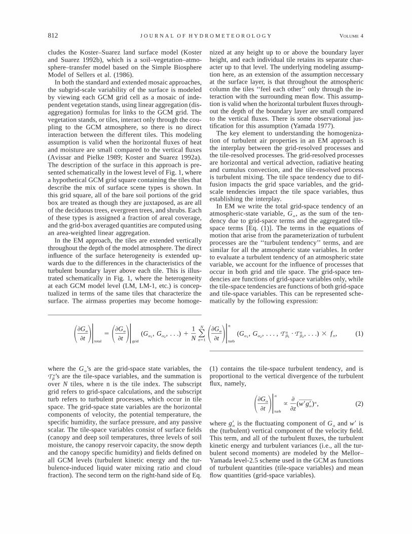
In EM we write the total grid-space tendency of anatmospheric-state variable, Ga, as the sum of the ten-dency due to grid-space terms and the aggregated tile-space terms [Eq. (1)]. The terms in the equations ofmotion that arise from the parameterization of turbulentprocesses are the ‘‘turbulent tendency’’ terms, and aresimilar for all the atmospheric state variables. In orderto evaluate a turbulent tendency of an atmospheric statevariable, we account for the influence of processes thatoccur in both grid and tile space. The grid-space ten-dencies are functions of grid-space variables only, whilethe tile-space tendencies are functions of both grid-spaceand tile-space variables. This can be represented sche-matically by the following expression:

nN]G ]G 1 ]Ga a a n n5 (G , G , . . .) 1 (G , G , . . . , T · T , . . .) 3 f , (1)Oa a a a b b n1 2 1 2 1 21 2) 1 2) 1 2)]t ]t N ]tn51total grid turb

where the Ga’s are the grid-space state variables, the’s are the tile-space variables, and the summation isnT b

over N tiles, where n is the tile index. The subscriptgrid refers to grid-space calculations, and the subscriptturb refers to turbulent processes, which occur in tilespace. The grid-space state variables are the horizontalcomponents of velocity, the potential temperature, thespecific humidity, the surface pressure, and any passivescalar. The tile-space variables consist of surface fields(canopy and deep soil temperatures, three levels of soilmoisture, the canopy reservoir capacity, the snow depthand the canopy specific humidity) and fields defined onall GCM levels (turbulent kinetic energy and the tur-bulence-induced liquid water mixing ratio and cloudfraction). The second term on the right-hand side of Eq.

(1) contains the tile-space turbulent tendency, and isproportional to the vertical divergence of the turbulentflux, namely,

n]G ]a n} (w9g9 ) , (2)a1 2)]t ]zturb

where is the fluctuating component of Ga and w9 isg9athe (turbulent) vertical component of the velocity field.This term, and all of the turbulent fluxes, the turbulentkinetic energy and turbulent variances (i.e., all the tur-bulent second moments) are modeled by the Mellor–Yamada level-2.5 scheme used in the GCM as functionsof turbulent quantities (tile-space variables) and meanflow quantities (grid-space variables).


FIG. 1. Schematic of the extended mosaic technique. The verticalaxis indicates the GCM model levels, where LM is the lowest leveland the level number increases as we ascend in the column.

In addition to the vertical extent of tile space, thereis another fundamental difference between the originalmosaic approach and EM. This difference is in the han-dling of the tile-space surface fluxes into the bottommodel layer. In EM it is the divergence of turbulentfluxes, or the turbulent tendency itself, which is com-puted in tile space and aggregated for use by the GCM,whereas in mosaic the surface fluxes are aggregated,and a grid-space divergence is computed.

In a full implementation of EM the atmospheric-statevariables would be retained at both tile space to computeturbulent diffusion and grid space to compute grid-spaceprocesses. The implementation of EM described above,however, does not retain the full set of atmospheric-state variables in tile space from one time step to thenext, rather the tile space boundary layer structure is

retained in the predicted turbulent second moments.This simplification may provide an additional homog-enizing influence. To the extent that the tile space struc-ture of the overlying boundary layer is preserved by theturbulent moments, EM as presently implemented willappropriately account for the vertical influence of sur-face heterogeneities.

3. The model blending height

In an analogy to the blending height concept, we de-fine here the model blending height (MBH) as the modellevel above the heterogeneous land surface at which itis assumed that the turbulent mixing has homogenizedthe airmass properties. This is the level above whichthe flow over the different tiles begins to appear uni-form. Each of the aggregation techniques describedabove implies a different extent of the vertical influenceof surface heterogeneity in the GCM. We can view thecomposite methodology as setting an MBH at theground and the mosaic approach as setting an MBH atthe top of the surface layer. The EM approach is theonly approach that has a variable MBH. The extensionof the concept of a blending height to larger scales wasbriefly mentioned in Bringfelt et al. (1999), where it isexplicitly stated that mosaic assumes that the blendingheight is at the surface layer, and that this might not bean adequate representation of the impact of surface het-erogeneity. The recognition that mosaic cannot accountfor the extended vertical influence of the land surfacevariability was noted earlier by Koster and Suarez(1992a). The limitations of mosaic in this regard wassuggested by the results of a study by Molders et al.(1996). They compared mosaic to an explicit subgrid-scale model, and reported that the differences are smallin the middle to upper troposphere and that these dif-ferences increase with proximity to the surface startinginside the atmospheric boundary layer. The extendedmosaic technique attempts to address these limitationsof mosaic discussed here.

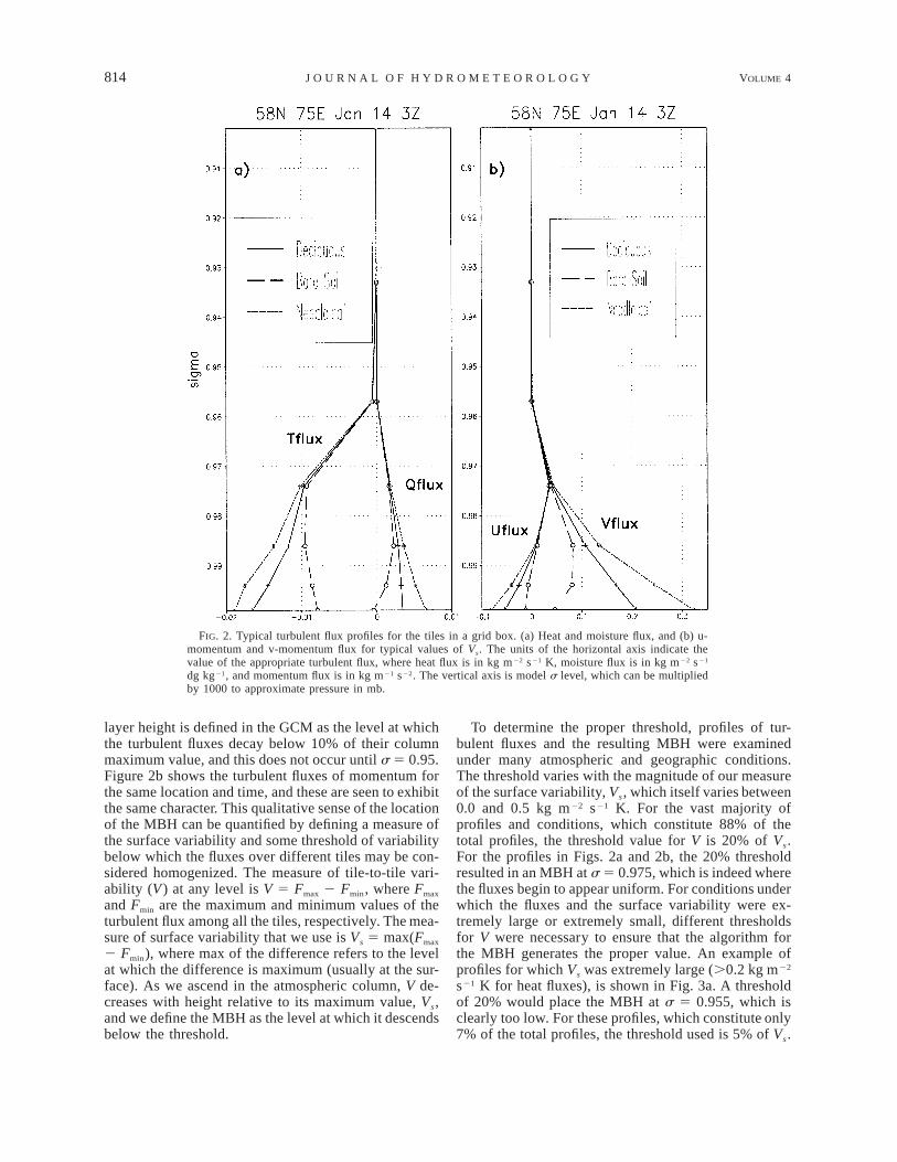
To define a measure of the MBH we examined theresults of a year-long GCM simulation using EM (seesection 4 for details). Typical profiles of the turbulentfluxes of temperature, momentum, and humidity overeach tile in a grid box are shown in Fig. 2. Figure 2ashows the profiles of and at 0300 UTC overw9u9 w9q9a grid point located in the northern steppes (588N, 758E).This particular grid box has three tiles, a broadleaf de-ciduous trees tile, a bare soil tile, and a needleaf treestile. The values of the flux emanating from the surfacelayer (those at the bottom s-level) are very differentfrom tile to tile. We also see that the differences in theturbulent fluxes between the tiles have been propagatedupward, as the fluxes are still distinct aloft. At higherlevels, values of approach each other until ap-w9u9proximately s 5 0.975 where the fluxes are almost in-distinguishable. At this ‘‘homogenized’’ level, however,the fluxes are still significant. The turbulent boundary


FIG. 2. Typical turbulent flux profiles for the tiles in a grid box. (a) Heat and moisture flux, and (b) u-momentum and v-momentum flux for typical values of Vs. The units of the horizontal axis indicate thevalue of the appropriate turbulent flux, where heat flux is in kg m22 s21 K, moisture flux is in kg m22 s21

dg kg21, and momentum flux is in kg m21 s22. The vertical axis is model s level, which can be multipliedby 1000 to approximate pressure in mb.

layer height is defined in the GCM as the level at whichthe turbulent fluxes decay below 10% of their columnmaximum value, and this does not occur until s 5 0.95.Figure 2b shows the turbulent fluxes of momentum forthe same location and time, and these are seen to exhibitthe same character. This qualitative sense of the locationof the MBH can be quantified by defining a measure ofthe surface variability and some threshold of variabilitybelow which the fluxes over different tiles may be con-sidered homogenized. The measure of tile-to-tile vari-ability (V) at any level is V 5 Fmax 2 Fmin, where Fmax

and Fmin are the maximum and minimum values of theturbulent flux among all the tiles, respectively. The mea-sure of surface variability that we use is Vs 5 max(Fmax

2 Fmin), where max of the difference refers to the levelat which the difference is maximum (usually at the sur-face). As we ascend in the atmospheric column, V de-creases with height relative to its maximum value, Vs,and we define the MBH as the level at which it descendsbelow the threshold.

To determine the proper threshold, profiles of tur-bulent fluxes and the resulting MBH were examinedunder many atmospheric and geographic conditions.The threshold varies with the magnitude of our measureof the surface variability, Vs, which itself varies between0.0 and 0.5 kg m22 s21 K. For the vast majority ofprofiles and conditions, which constitute 88% of thetotal profiles, the threshold value for V is 20% of Vs.For the profiles in Figs. 2a and 2b, the 20% thresholdresulted in an MBH at s 5 0.975, which is indeed wherethe fluxes begin to appear uniform. For conditions underwhich the fluxes and the surface variability were ex-tremely large or extremely small, different thresholdsfor V were necessary to ensure that the algorithm forthe MBH generates the proper value. An example ofprofiles for which Vs was extremely large (.0.2 kg m22

s21 K for heat fluxes), is shown in Fig. 3a. A thresholdof 20% would place the MBH at s 5 0.955, which isclearly too low. For these profiles, which constitute only7% of the total profiles, the threshold used is 5% of Vs.


FIG. 3. Turbulent flux profiles neccessitating extreme threshold values. (a) Heat and momentum flux fora case in which Vs is large, and (b) heat flux for a case in which Vs is small. The units of the horizontalaxis indicate the value of the appropriate turbulent flux, where heat flux is in kg m22 s21 K, and momentumflux is in kg m21 s22. The vertical axis is model s level, which can be multiplied by 1000 to approximatepressure in mb.

TABLE 1. Range of surface variability Vs calculated with turbulentheat fluxes in units of kg m22.

Vs Threshold %Percent of cases

included

Vs , 0.0010.001 , Vs , 0.0060.006 , Vs , 0.2

0.2 , Vs

806520

5

14

887

An example of profiles for which the fluxes and thesurface variability were extremely small (,0.006 kgm22 s21 K), is shown in Fig. 3b. The 20% thresholdwould set the MBH at s 5 0.935, which is clearly toofar above the level at which the fluxes merge. For theseprofiles, which constitute roughly 4% of the total pro-files, the threshold used is 65% of Vs, and the MBH isat s 5 0.985. Finally, another threshold of 80% of Vs

was needed for a very small number of profiles, roughly1% of the cases, in which Vs is near zero (,0.001 kg

m22 s21 K). The thresholds for each range of Vs arelisted in Table 1. With this choice of thresholds, alongwith our choice of Vs as the measure of surface vari-ability, we chose to define the MBH based on heat fluxesalone. Calculations of the MBH were also performedbased on the moisture and momentum fluxes, and theresulting values were almost indistinguishable fromthose based on the heat fluxes.

Our algorithm to estimate the MBH is consistent withthe ideas used to estimate the blending height (Mahrt2000). These different approaches to assessing a mea-sure of the level of the blending height all involve somemeasure of the surface variability and the level at whichit decays below some threshold. One such measure in-volves a threshold value for the variance of the skintemperature normalized by some reference potentialtemperature, /Q0. Another measure involves the var-sTs

iance of some turbulent flux divided by the flux, sF/F.In the context of our GCM study using the variance asthe measure of surface variability is not suitable for a


TABLE 2. GEOS-Terra GCM surface type designation.

Type Vegetation designation

12345

Broadleaf evergreen treesBroadleaf deciduous treesNeedleleaf treesGround coverBroadleaf shrubs

6789

10100

Dwarf trees (tundra)Bare soilDesert (bright)GlacierDesert (dark)Ocean

mosaic scheme involving three to four tiles in a gridbox. Just like our measure of the surface variability,these measures of surface variability do not depend ex-clusively on the vegetation characteristics themselves.The physical characteristics of the land surface, such asthe surface roughness and the soil hydraulic conductiv-ity, are constant in time or vary on monthly timescales.The measures defined earlier in this paper depend onthe local conditions as well, which may vary on manyshorter and longer timescales. For example, under ex-treme cold atmospheric conditions the surface fluxes areminimal, and under wet conditions the evaporation pro-ceeds at its potential rate. Either of these conditions willresult in the suppression of any differences in physicalcharacteristics and a reduced surface variability.

4. Characterization of the MBH

We now examine the spatial and temporal variabilityof the MBH and the relationship with other quantitiesusing a year-long segment of a 27-month simulationperformed with the EM technique as implemented inthe GEOS-Terra GCM. The simulation is from Decem-ber 1997 to March 2000 and is forced with observedweekly varying sea surface temperatures. The surfacetypes used in this experiment are listed in Table 2. Thedata for percent of the grid cell occupied by any surfacetype were derived from the surface classification of De-fries and Townshend (1994), and information about thelocation of permanent ice was obtained from the clas-sifications of Dorman and Sellers (1989). The resultingvegetation map can be found Molod and Salmun (2002;their Fig. 2). In general, most grid boxes are charac-terized by approximately four different scene types(tiles). Several of the vegetation characteristics—name-ly, the leaf area index, greenness fraction, and surfaceroughness length—vary from month to month, whilethe others are constant throughout the year. The simu-lation results of 1998, for which an extensive diagnosticoutput in tile space was generated, were used to examinethe EM technique by analyzing the behavior of theMBH. We focus on the relationships between the MBHand other relevant physical parameters, such as the plan-etary boundary layer (PBL) height, the surface tem-

perature and fluxes, and the type and distribution ofunderlying vegetation. To illustrate these relationships,we will present monthly averages of global fields andannual time series for representative points around theglobe.

December–January–February (DJF) seasonal meanvalues of MBH, PBL, and the ratio MBH/PBL, givenin pressure thickness above the surface, are shown inFig. 4. The PBL height in the GCM is the level at whichthe turbulent kinetic energy decays below 10% of itsmaximum value in the air column, and there is thereforeno a priori relationship between the MBH and the PBLheight. The plots in Fig. 4 show that the MBH is var-iable, is above the surface layer, and is related to thePBL height but does not follow it exactly. The valuesof MBH range from 10 to near 40 mb (100–400 m,approximately). The geographic locations where theMBH is low, which are indicated by the blue areas ofFig. 4a, are the Tibetan Plateau, the Rocky Mountains,the Amazon basin, central Africa, and Siberia. The lowMBH corresponds to low PBL values (the light blueregions in Fig. 4b) in all of these regions except for theAmazon, where the low MBH is associated with a rel-atively homogeneous terrain. Over the regions totallysnow-covered in wintertime, the low MBH values mayalso be due to the potentially homogenizing effect ofthe snow. Regions where the MBH is high during DJFare the Southern Hemisphere midlatitude areas, whereit is summertime, and where the PBL values are alsohigh. There is another band of high MBH values atapproximately 458N latitude across the North American,European, and Asian continents. There is some indi-cation of a local maximum in PBL height at these lo-cations, as well as a transition of vegetation types atthat latitude. There is also a local maximum in MBHin the Sahel region of Africa, related to the behavior ofthe PBL.

The ratio of MBH to PBL is always less than 1 (Fig.4c), ranging from 0.05 to greater than 0.9, indicatingthat the MBH is always below the PBL. The global meanratio is approximately 0.2–0.3. There is a monotonicdecrease in the ratio of MBH to PBL in the NorthernHemisphere from high latitudes (ratio near 0.9) to lowlatitudes (ratio near 0.15), except in the eastern UnitedStates. The large change in ratio is the result of a PBLthickness, which increases more rapidly than the MBHfrom north to south across these regions. In general, theratio is low in the Southern Hemisphere, due to the highsummertime PBL values. There is a local minimum inthe ratio over the eastern United States, which corre-sponds to the local maximum in the PBL height (witha similar contour shape). In addition, there is a localminimum in the ratio over Sahel, where the PBL heightis very high (greater than 300 mb). The ratio increasesnorth of Sahel, due to the more rapid dropoff of thePBL height than the MBH.

The corresponding plots for June–July–August (JJA)are shown in Fig. 5. These plots also show that the MBH


FIG. 4. Dec–Jan–Feb averaged model blending height and planetary boundary layer depth. (a)Model blending height in mb, (b) planetary boundary layer depth, also in mb, and (c) ratio ofMBH to PBL (dimensionless). The contour levels are indicated in the color bar to the right.

is variable, and lies above the surface layer and insidethe PBL. Some of the areas where the MBH is highcorrespond to high PBL values, such as the deserts ofSahara, Gobi, Saudi Arabia, and the southwestern Unit-ed States, and regions in southern Africa and just southof the Amazon. An additional band of high MBH valuesexists at approximately 358–408N latitude, stretchingacross Canada, Europe, and Asia. These high MBH val-ues do not correspond to local maxima in the PBLheight, rather they correspond in the shape of the con-tour to areas where there is a change in the nature ofthe vegetation (see Molod and Salmun 2002, their Fig.2). In these regions the vegetation changes from a com-bination of bare soil and dwarf trees to predominantlyneedleleaf trees. The geographical locations where the

MBH is low are the Amazon, where the variability ofthe vegetation is small, and the Andes and the TibetanPlateau, where the altitude and the cold temperatureslimit the height of the PBL. There is also a local min-imum in MBH in the southern tip of Africa, and anotherin central South America, just south of the local max-imum. The ratio of MBH to PBL values is generallylower than in the Northern Hemisphere wintertime, withthe lowest values (less than 20%) corresponding to thehighest values of PBL height. Except for southern Af-rica, the ratios are higher in the Southern Hemisphere(winter hemisphere) than in the summer hemisphere.

In general the MBH values differ more from the PBLheight values in JJA than in DJF. The evolution of thesefields throughout the year (not shown) indicates that the


FIG. 5. The same as in Fig. 4 except for Jun–Jul–Aug.

latitude of maximum MBH in the Northern Hemispheretraverses poleward in the wintertime and equatorwardin summertime. This can be seen in the DJF and JJAMBH fields, where, for example, over Asia, the locationof high MBH values (shaded orange in Fig. 4, 30–35mb) is near 608N latitude in DJF, and moves south tonear 408N in JJA (Fig. 5). The same summer–wintertraverse can be seen in Africa and South America fromDJF to JJA, but in the Southern Hemisphere the pole-ward shift occurs in the summertime (December).

To gain some further insight into the relationship be-tween the MBH and the PBL, we examine scatterplotsof seasonal mean MBH versus PBL for all land points.Figure 6 shows this plot for JJA. In general, the MBHincreases with PBL height, except for high (greater than200 mb) PBL values, where there is a leveling off of

the MBH. These high PBL values occur over desertareas, where the variability of the surface vegetation issmall (90% desert and 10% broadleaf shrubs), and in asmall area in the Amazon, the behavior of which isexamined later in this paper. Although there is a lineartrend between MBH and PBL for the lower PBL values,the spread about the representative line is greater thantwo standard deviations. This spread indicates that theMBH does not depend simply on PBL height, but is theresult of a more complex interplay among differentphysical processes. Similar behavior was observed inDJF (not shown).

We examined the involvement of the other physicalprocesses in determining the MBH by examining similarscatterplots for other variables. Figure 7 shows the scat-terplot of JJA MBH against Tc. It shows that the MBH


FIG. 6. MBH vs PBL scatterplot (mb) for Jun, Jul, and Augmonthly mean values over all land points.

FIG. 7. MBH (mb) vs canopy temperature (K) scatterplot for Jun,Jul, and Aug monthly mean values over all land points. Points overtropical rain forests are colored red.

increases with Tc, with MBH values ranging from near10 to near 45 mb over a temperature range of 260 to310 K. The exception to this behavior is a small groupof points, colored in red, at relatively warm canopytemperatures (just below 300 K), for which the MBHvalues are near 10–15 mb, rather than closer to 30 mb,as the global trend would have dictated. These pointsare all characterized as tropical rain forest, and the re-lationship between MBH and Tc over this type of dense-ly forested terrain is markedly different from the rela-tionship over other types of soil and vegetation. Forthese points, the MBH varies much more rapidly withtemperature and ranges from 13 to 42 mb over a Tc

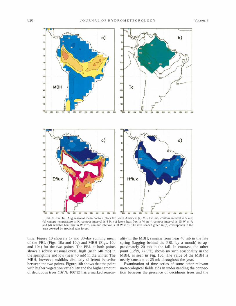
range of 295 to 300 K. In the tropical rain forests, thelow MBH (and lower Tc) points are characterized byvery high levels of evaporation, and the high MBH (andhigher Tc) points have almost no evaporation. We il-lustrate this behavior with contour plots of MBH, Tc,and turbulent surface fluxes over the Amazon region,Figs. 8a–d, where we see that the areas of high MBH(Fig. 8a) correspond to the areas of low evaporation(Fig. 8c). At the lower temperatures, the evaporationlevels suppress the sensible heat flux (available energyat the surface is released through evaporation, primarilythrough evapotranspiration) and the MBH is lower. Incontrast, at the higher temperatures (beyond the model-specified threshold), the evaporation is suppressed toconserve leaf and plant moisture, the sensible heat fluxis increased, and the MBH is higher. This correspon-dence to the sensible heat flux is seen in Fig. 8d.

Similar scatterplots of MBH versus sensible heat flux(not shown) show that the global relationship betweenthe MBH and the sensible heat flux is linear in character,with MBH increasing with sensible heat. This is as ex-

pected, given that the sensible heat flux is the majorcontributor to the boundary layer bouyancy and tur-bulence that determines the PBL height. This relation-ship between MBH and sensible heat flux is independentof the choice of surface variability used to define theMBH. The linear relationship holds even when the MBHis defined based on the variability of surface latent heatflux or momentum flux.

In addition to a relationship between the MBH andthe local characteristics of the turbulence, the behaviorof the MBH also depends on the type and variability ofsurface vegetation. We demonstrate this relationshipwith a year-long time series of the MBH and PBL attwo characteristic points in the region of the Indian–Asian monsoon. These points and their vegetation char-acteristics are indicated in Fig. 9, which shows a shadedmap of the fractional area covered by vegetation typesother than the dominant type. This is a measure of thevariability of vegetation in the grid box. The first pointis in southern Asia (168N, 1008E) and is characterizedby 60.0% ground cover, 14.8% broadleaf evergreentrees, 14.3% broadleaf deciduous trees, 8.9% bare soil,and 2.0% dwarf trees. This point has the higher off-dominant percent of coverage of the two points, and isalso differentiated from the other point by the presenceof the deciduous trees. The second point is on the Indiansubcontinent (128N, 77.58E) and is characterized by80.5% ground cover, 9.8% bare soil, 4.7% dwarf trees,3.1% broadleaf deciduous trees, and 1.9% broadleaf ev-ergreen trees. This point has the lower off-dominantfraction and almost no deciduous trees. Both of thesepoints are in climatologically similar regimes, governedby a monsoonal flow and relatively dry in the winter-


FIG. 8. Jun, Jul, Aug seasonal mean contour plots for South America. (a) MBH in mb, contour interval is 5 mb;(b) canopy temperature in K, contour interval is 4 K; (c) latent heat flux in W m22, contour interval is 15 W m22;and (d) sensible heat flux in W m22, contour interval is 30 W m22. The area shaded green in (b) corresponds to thearea covered by tropical rain forest.

time. Figure 10 shows a 1- and 30-day running meanof the PBL (Figs. 10a and 10c) and MBH (Figs. 10band 10d) for the two points. The PBL at both pointsshows a robust seasonal cycle, high (near 140 mb) inthe springtime and low (near 40 mb) in the winter. TheMBH, however, exhibits distinctly different behaviorbetween the two points. Figure 10b shows that the pointwith higher vegetation variability and the higher amountof deciduous trees (168N, 1008E) has a marked season-

ality in the MBH, ranging from near 40 mb in the latespring (lagging behind the PBL by a month) to ap-proximately 20 mb in the fall. In contrast, the otherpoint (128N, 77.58E) shows no such seasonality in theMBH, as seen in Fig. 10d. The value of the MBH isnearly constant at 25 mb throughout the year.

Examination of time series of some other relevantmeteorological fields aids in understanding the connec-tion between the presence of deciduous trees and the


FIG. 9. Percent of grid box covered by nondominant vegetation for southern Asia. The two illustrated gridpoints are indicated by the blue and red boxes and by the description of vegetation characteristics.

MBH seasonality. Figure 11 shows the 1- and 30-dayrunning means of the latent heat flux (Figs. 11a,b), can-opy temperature (Figs. 11c,d), precipitation (Figs.11e,f), and sensible heat flux (Figs. 11g,h) for bothpoints. The similarity of the precipitation patterns (Figs.11e,f) and canopy temperature patterns (Figs. 11c,d) atboth points demonstrates that they are in the same cli-mate regime. Figures 11a,b show that the latent heatflux over the point with deciduous trees is almost com-pletely suppressed during the months when the treeshave no leaves. This results in a sharper increase inlatent flux during the springtime. In contrast, at 128N,77.58E (the point with no deciduous trees and low sur-face variability) the latent flux is small in wintertimebut is not completely suppressed, and the contrast be-

tween winter and springtime levels is not as marked.Consistent with the behavior of the latent heat flux, Figs.11g,h show that the sensible heat flux at 168N, 1008Eis higher in wintertime than the sensible heat at 128N,77.58E.

Examination of other points in this climatological re-gime revealed that the presence of deciduous trees aloneis insufficient to generate a high seasonality in the MBH.High surface variability is necessary as well. For ex-ample, the grid box at 108N, 77.58E has deciduous treesbut low surface variability, is characterized by 80.0%ground cover, 9.0% broadleaf deciduous trees, 10.0%bare soil, and 1.0% dwarf trees, and shows no season-ality in the MBH, despite a marked seasonality in thePBL. In other words, the variability and the presence


FIG. 10. Time series of PBL and MBH height in mb for 1008E, 168N, (a) and (b), respectively,and for 77.58E, 128N, (c) and (d), respectively. Each panel contains 1- and 30-day running means.

of deciduous trees is needed for the MBH to exhibit astrong seasonal cycle.

5. Summary and conclusions

The study of the extended mosaic (EM) techniquepresented here is aimed at developing a better tool tosimulate and understand the direct (aggregation) effectsof the interactions between a heterogeneous land surfaceand the climate. This technique allows the influence ofthe surface heterogeneities to extend upward into the

turbulent boundary layer by assuming that the concep-tualization of surface heterogeneity as a mosaic of in-dependent vegetation stands is applicable throughout theatmospheric column. The additional degree of freedomof the system, that of allowing the vertical extent of theinfluence of surface heterogeneities to be determinedinternally, has the potential to afford a better charac-terization of the land–atmosphere interactions.

Simulations with this technique revealed that the pro-files of turbulent fluxes over each tile in a grid box differnear the ground and become homogenized at some level


FIG. 11. Time series of meteorological fields for 77.58E, 128N and 1008E, 168N. (a), (c), (e), (g) Latent heat flux in W m22, canopytemperature in K, precipitation in mm day21, and sensible heat flux in W m22, respectively, for 77.58E, 128N. (b), (d), (f ), (h) The correspondingplots for 1008E, 168N. Each panel contains 1- and 30-day running means.

aloft. This behavior allows the definition of a modelblending height (MBH) as the level where the homog-enization takes place. We emphasize that the EM al-gorithm does not require that the turbulent fluxes be-come homogenized, hence the blending is a result ofthe simulations with EM. The MBH varies between 50and 500 m, and is generally about one-third of the PBLheight. The exact ratio depends on meteorological con-ditions, location, and the amount of variability in theland scene type.

Examination of the relationship among the MBH andother meteorological variables shows that seasonal meanvalues of the MBH and PBL height exhibit similar spa-tial patterns in warm and dry regions, and differ morein the Northern Hemisphere wintertime and over rela-tively homogeneous terrain. The MBH increases grad-ually with PBL height, sensible heat flux, and canopytemperature through moderate to warm values, althoughthe spread of values about these trends is substantial.This spread is indicative of the complexity of the de-

pendence of the MBH on local conditions, and severalexamples of this complexity were presented.

The dependence of the MBH on the canopy temper-ature increases dramatically for temperatures near 300K. This is related to the behavior of the latent heat flux,which is high for temperatures just below 300 K, andis suppressed (infinite stomatal resistance) when the can-opy temperature exceeds a vegetation-dependent thresh-old (usually near 300 K). When the evaporation is high,the MBH is low, and when the available surface energyis released as sensible rather than latent heat flux, theMBH is elevated. This results in the sharp increase ofMBH with canopy temperature in regions where evap-oration dominates the surface energy balance.

The MBH was also found to depend on the variabilityand types of underlying vegetation. The presence ofdeciduous trees in the mix of tiles, in addition to highlevels of variability in scene type, was shown to beassociated with in an increased seasonality of the MBH.An example of this behavior was presented by exam-


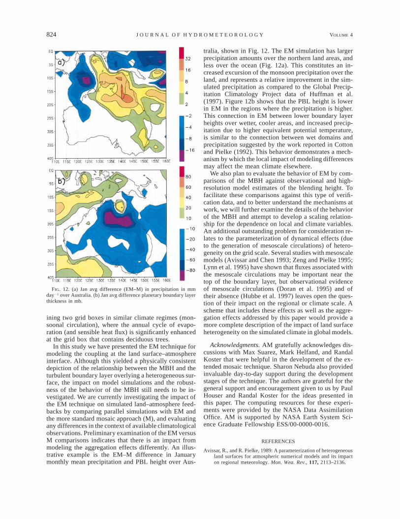
FIG. 12. (a) Jan avg difference (EM–M) in precipitation in mmday21 over Australia. (b) Jan avg difference planetary boundary layerthickness in mb.

ining two grid boxes in similar climate regimes (mon-soonal circulation), where the annual cycle of evapo-ration (and sensible heat flux) is significantly enhancedat the grid box that contains deciduous trees.

In this study we have presented the EM technique formodeling the coupling at the land surface–atmosphereinterface. Although this yielded a physically consistentdepiction of the relationship between the MBH and theturbulent boundary layer overlying a heterogeneous sur-face, the impact on model simulations and the robust-ness of the behavior of the MBH still needs to be in-vestigated. We are currently investigating the impact ofthe EM technique on simulated land–atmosphere feed-backs by comparing parallel simulations with EM andthe more standard mosaic approach (M), and evaluatingany differences in the context of available climatologicalobservations. Preliminary examination of the EM versusM comparisons indicates that there is an impact frommodeling the aggregation effects differently. An illus-trative example is the EM–M difference in Januarymonthly mean precipitation and PBL height over Aus-

tralia, shown in Fig. 12. The EM simulation has largerprecipitation amounts over the northern land areas, andless over the ocean (Fig. 12a). This constitutes an in-creased excursion of the monsoon precipitation over theland, and represents a relative improvement in the sim-ulated precipitation as compared to the Global Precip-itation Climatology Project data of Huffman et al.(1997). Figure 12b shows that the PBL height is lowerin EM in the regions where the precipitation is higher.This connection in EM between lower boundary layerheights over wetter, cooler areas, and increased precip-itation due to higher equivalent potential temperature,is similar to the connection between wet domains andprecipitation suggested by the work reported in Cottonand Pielke (1992). This behavior demonstrates a mech-anism by which the local impact of modeling differencesmay affect the mean climate elsewhere.

We also plan to evaluate the behavior of EM by com-parisons of the MBH against observational and high-resolution model estimates of the blending height. Tofacilitate these comparisons against this type of verifi-cation data, and to better understand the mechanisms atwork, we will further examine the details of the behaviorof the MBH and attempt to develop a scaling relation-ship for the dependence on local and climate variables.An additional outstanding problem for consideration re-lates to the parameterization of dynamical effects (dueto the generation of mesoscale circulations) of hetero-geneity on the grid scale. Several studies with mesoscalemodels (Avissar and Chen 1993; Zeng and Pielke 1995;Lynn et al. 1995) have shown that fluxes associated withthe mesoscale circulations may be important near thetop of the boundary layer, but observational evidenceof mesoscale circulations (Doran et al. 1995) and oftheir absence (Hubbe et al. 1997) leaves open the ques-tion of their impact on the regional or climate scale. Ascheme that includes these effects as well as the aggre-gation effects addressed by this paper would provide amore complete description of the impact of land surfaceheterogeneity on the simulated climate in global models.

Acknowledgments. AM gratefully acknowledges dis-cussions with Max Suarez, Mark Helfand, and RandalKoster that were helpful in the development of the ex-tended mosaic technique. Sharon Nebuda also providedinvaluable day-to-day support during the developmentstages of the technique. The authors are grateful for thegeneral support and encouragement given to us by PaulHouser and Randal Koster for the ideas presented inthis paper. The computing resources for these experi-ments were provided by the NASA Data AssimilationOffice. AM is supported by NASA Earth System Sci-ence Graduate Fellowship ESS/00-0000-0016.

REFERENCES

Avissar, R., and R. Pielke, 1989: A parameterization of heterogeneousland surfaces for atmospheric numerical models and its impacton regional meteorology. Mon. Wea. Rev., 117, 2113–2136.


——, and F. Chen, 1993: Development and analysis of prognosticequations for mesoscale kinetic energy and mesoscale (subgridscale) fluxes for large-scale atmospheric models. J. Atmos. Sci.,50, 3751–3774.

——, and T. Schmidt, 1998: An evaluation of the scale at whichground-surface heat flux patchiness affects the convectiveboundary layer using large-eddy simulations. J. Atmos. Sci., 55,2666–2689.

Bringfelt, B., M. Heikimheimo, N. Gustafsson, V. Perov, and A. Lind-roth, 1999: A new land-surface treatment for HIRLAM—Com-parisons with NOPEX measurements. Agric. For. Meteor., 98–9, 239–256.

Brutsaert, W., 1998: Land-surface water vapor and sensible heat flux:Spatial variability, homogeneity, and measurement scales. WaterResour. Res., 34, 2233–2442.

Chen, F., and R. Avissar, 1994: Impact of land-surface moisture var-iability on local shallow convective cumulus and precipitationin large-scale models. J. Appl. Meteor., 33, 1382–1401.

Claussen, M., 1995: Flux aggregation at large scales: On the limitsof validity of the concept of blending height. J. Hydrol., 166,371–382.

Cotton, W. R., and R. A. Pielke, 1992: Human Impacts on Weatherand Climate. Cambridge University Press, 288 pp.

DeFries, R. S., and J. R. G. Townshend, 1994: NDVI-derived landcover classification at global scales. Int. J. Remote Sens., 15,3567–3586.

Dickinson, R., A. Henderson-Sellers, P. Kennedy, and M. Wilson,1986: Biosphere–Atmosphere Transfer Scheme (BATS) forNCAR Community Climate Model. Tech. Note TN 2751STR,National Center for Atmospheric Research, Boulder, CO, 69 pp.

Doran, J. C., W. J. Shaw, and J. M. Hubbe, 1995: Boundary layercharacteristics over areas of inhomogeneous surface fluxes. J.Appl. Meteor., 34, 559–571.

Dorman, J. L., and P. J. Sellers, 1989: A global climatology of albedo,roughness length and stomatal resistance for atmospheric generalcirculation models as represented by the Simple Biosphere Mod-el (SiB). J. Appl. Meteor., 28, 833–855.

Entekhabi, D., and P. S. Eagleson, 1989: Land surface hydrologyparameterization for atmospheric general circulation models in-cluding subgrid scale spatial variability. J. Climate, 2, 816–831.

Giorgi, F., and R. Avissar, 1997: Representation of heterogeneityeffects in earth system modeling: Experience from land surfacemodeling. Rev. Geophys., 35, 413–438.

Helfand, H. M., and J. C. Labraga, 1988: Design of a non-singularlevel 2.5 second-order closure model for the prediction of at-mospheric turbulence. J. Atmos. Sci., 45, 113–132.

——, and S. D. Schubert, 1995: Climatology of the simulated GreatPlains low-level jet and its contribution to the continental mois-ture budget of the United States. J. Climate, 8, 784–806.

Hess, G. D., and B. J. McAvaney, 1998: Realisability constraints forland surface schemes. Global Planet. Change, 19, 241–245.

Hubbe, J. M., J. C. Doran, J. C. Liljegren, and W. J. Shaw, 1997:Observations of spatial variations of boundary layer structureover the Southern Great Plains Cloud and Radiation Testbed. J.Appl. Meteor., 36, 1221–1231.

Huffman, G. J., and Coauthors, 1997: The Global Precipitation Cli-matology Project (GPCP) Combined Precipitation Dataset. Bull.Amer. Meteor. Soc., 78, 5–20.

Koster, R. D., and M. J. Suarez, 1992a: A comparitive analysis oftwo land surface heterogeneity representations. J. Climate, 5,1379–1390.

——, and ——, 1992b: Modeling the land surface boundary in cli-mate models as a composite of independant vegetation stands.J. Geophys. Res., 97, 2697–2715.

Lynn, B. H., F. Abramopoulos, and R. Avissar, 1995: Using similaritytheory to parameterize mesoscale heat fluxes generated by land-scape discontinuities in GCMs. J. Climate, 8, 932–951.

Mahrt, L., 1996: The bulk aerodynamic formulation over heteroge-neous surfaces. Bound.-Layer Meteor., 78, 87–119.

——, 2000: Surface heterogeneity and vertical structure of the bound-ary layer. Bound.-Layer Meteor., 96, 33–62.

Mason, P. J., 1988: The formation of areally-averaged roughnesslength. Quart. J. Roy. Meteor., Soc., 114, 399–420.

Molders, N., A. Raabe, and G. Tetzlaff, 1996: A comparison of twostrategies on land surface heterogeneity used in a mesoscale bmeteorological model. Tellus, 48A, 733–749.

Molod, A., 1999: The land surface component in GEOS: Model for-mulation. DAO Office Note 1999-03, Office Note Series onGlobal Modeling and Data Assimilation, Goddard Space FlightCenter, Greenbelt, MD, 21 pp.

——, and H. Salmun, 2002: A Global assessment of the mosaicapproach to modeling land surface heterogeneity. J. Geophys.Res., 107, 4217, doi:10.1029/2001JD000588.

Parlange, M. B., and G. Katul, 1995: Watershed scale shear stressfrom tethersonde wind profile measurements under near neutraland unstable atmospheric stability. Water Resour. Res., 31, 961–968.

Sellers, P. J., Y. Mintz, Y. C. Sud, and A. Dalcher, 1986: A SimpleBiosphere Model (SiB) for use within general circulation models.J. Atmos. Sci., 43, 505–531.

Viterbo, P., and A. C. M. Beljaars, 1995: An improved land surfaceparameterization scheme in the ECMWF Model and its vali-dation. J. Climate, 8, 2716–2748.

Wieringa, J., 1986: Roughness-dependent geographical interpolationof surface wind speed averages. Quart. J. Roy. Meteor. Soc.,112, 867–889.

Yamada, T., 1977: A numerical simulation of pollutant dispersion ina horizontally-homogeneous atmospheric boundary layer. Atmos.Environ., 11, 1015–1024.

Zeng, X., and R. A. Pielke, 1995: Landscape-induced atmosphericflow and its parameterization in large-scale numerical models.J. Climate, 8, 1156–1177.

a new look at modeling surface heterogeneity: extending

Documents