a new duality based approach for the problem of locating a
TRANSCRIPT

A new Duality Based Approach
for the Problem of Locating a
Semi-Obnoxious Facility
Dissertation
zur Erlangung des akademischen Grades
doctor rerum naturalium (Dr. rer. nat.)
der
Naturwissenschaftlichen Fakultat II
Chemie, Physik und Mathematik
der Martin-Luther-Universitat
Halle-Wittenberg,
vorgelegt von
Frau Dipl. Math. Andrea Wagner
geboren am 29. Juli 1983 in Wolmirstedt
Halle (Saale), 06. August 2014

Gutachter:
1. Prof. Dr. Christiane Tammer
2. Prof. Dr. Juan-Enrique Martınez-Legaz
3. Prof. Dr. Kathrin Klamroth
Tag der Verteidigung: 23. Januar 2015

Contents
1 Introduction 1
2 Literature Overview and Classification 5
3 Formulation of the Location Problem 11
4 Preliminaries 13
4.1 Convex Sets and Cones . . . . . . . . . . . . . . . . . . . . . . . . . . . . . . . . 13
4.2 Convex Functions . . . . . . . . . . . . . . . . . . . . . . . . . . . . . . . . . . . . 16
4.3 Elementary Convex Sets . . . . . . . . . . . . . . . . . . . . . . . . . . . . . . . . 25
4.4 D.C. Programming Problems and Toland-Singer Duality . . . . . . . . . . . . . . 27
5 Duality Assertions for Location Problems with Obnoxious Facilities 31
5.1 Existence of Finite Optimal Solutions . . . . . . . . . . . . . . . . . . . . . . . . 32
5.2 Geometrical Properties, Duality Statements and Optimality Conditions . . . . . 34
5.3 Discretization Results . . . . . . . . . . . . . . . . . . . . . . . . . . . . . . . . . 41
6 An Assignment between Primal and Dual Elements 43
7 An Application of Benson’s Algorithm 47
8 Consideration of Polyhedral Constraints 55
8.1 Geometrical Properties . . . . . . . . . . . . . . . . . . . . . . . . . . . . . . . . . 57
8.2 Existence of Finite Optimal Solutions . . . . . . . . . . . . . . . . . . . . . . . . 59
8.3 Optimality Conditions and Discretization Results . . . . . . . . . . . . . . . . . . 60
8.4 Example . . . . . . . . . . . . . . . . . . . . . . . . . . . . . . . . . . . . . . . . . 62
9 An Algorithm for Location Problems with Obnoxious Facilities 65
9.1 Determination of Grid Points w.r.t. Attraction . . . . . . . . . . . . . . . . . . . 65
9.2 Determination of Grid Points w.r.t. Repulsion . . . . . . . . . . . . . . . . . . . . 66
9.3 Solving the Location Problem with Obnoxious Facilities . . . . . . . . . . . . . . 71
9.4 Example . . . . . . . . . . . . . . . . . . . . . . . . . . . . . . . . . . . . . . . . . 74

iv Contents
9.5 The Special Case of no Repulsion . . . . . . . . . . . . . . . . . . . . . . . . . . . 79
9.6 An Algorithm for Solving the Constrained Problem with Obnoxious Facilities . . 79
10 A Matlab Implementation for the 2-Dimensional Case 83
10.1 Input Arguments . . . . . . . . . . . . . . . . . . . . . . . . . . . . . . . . . . . . 84
10.2 Output Arguments . . . . . . . . . . . . . . . . . . . . . . . . . . . . . . . . . . . 87
10.3 Subroutines of the Matlab Implementation . . . . . . . . . . . . . . . . . . . . . . 88
10.4 Examples . . . . . . . . . . . . . . . . . . . . . . . . . . . . . . . . . . . . . . . . 95
11 Conclusion 107
Index 108
Bibliography 111


List of Figures
4.1 Dual normal cones and cones generated by primal exposed faces . . . . . . . . . 26
4.2 Primal Construction Grid for Example 4.18 . . . . . . . . . . . . . . . . . . . . . 27
5.1 Dual construction grids for different choices of weights. . . . . . . . . . . . . . . . 39
6.1 Assignment between primal and dual elements . . . . . . . . . . . . . . . . . . . 46
8.1 Primal and dual grids w.r.t. attraction in case of polyhedral constraints. . . . . . 64
9.1 Primal and dual grid w.r.t. repulsion in case of Manhattan distances. . . . . . . . 70
9.2 Example for the primal algorithm . . . . . . . . . . . . . . . . . . . . . . . . . . . 77
9.3 Example for the dual algorithm . . . . . . . . . . . . . . . . . . . . . . . . . . . . 78
10.1 Primal and dual plot for Example 10.4. . . . . . . . . . . . . . . . . . . . . . . . 96
10.2 Primal and dual plot for Example 10.5. . . . . . . . . . . . . . . . . . . . . . . . 98
10.3 Primal and dual plot for Example 10.6. . . . . . . . . . . . . . . . . . . . . . . . 100
10.4 Primal and dual plot for Example 10.7. . . . . . . . . . . . . . . . . . . . . . . . 102
10.5 Primal and dual plot for Example 10.9. . . . . . . . . . . . . . . . . . . . . . . . 105

Notation
Rn+ {x ∈ Rn| x ≥ 0}
a1, . . . , aM ∈ Rn Attracting facilities
w1, . . . , wM > 0 Weights of attracting facilities
B1, . . . , BM ⊆ Rn Unit balls assigned to the attracting facilities
B∗1, . . . , B
∗M ⊆ Rn Dual unit balls of B1, . . . , BM
g : Rn → R Weighted sum of distances to attracting facilities
gH : Rn → R ∪ {+∞} Weighted sum of distances to attracting facilities considering a
constraints set H
a1, . . . , aM ∈ Rn Repulsive facilities
w1, . . . , wM > 0 Weights of repulsive facilities
B1, . . . , BM ⊆ Rn Unit balls assigned to the repulsive facilities
B∗1, . . . , B∗M ⊆ Rn Dual unit balls of B1, . . . , BM
h : Rn → R Weighted sum of distances to repulsive facilities
(P ) Unconstrained location problem with obnoxious facilities
I Primal grid points w.r.t. attraction
I Primal grid points w.r.t. repulsion
G Primal grid w.r.t. attraction
G Primal grid w.r.t. repulsion
X Set of optimal points of (P)
(D) Toland-Singer-dual problem of (P)
ID Dual grid points w.r.t. attraction
ID Dual grid points w.r.t. repulsion
GD Dual grid w.r.t. attraction
GD Dual grid w.r.t. repulsion
Y Set of optimal points of (D)
H Convex polyhedral constraints set
(PH) Constrained location problem with obnoxious facilities
IH Primal constrained grid points w.r.t. attraction
GH
Primal constrained grid w.r.t. attraction
XH Set of optimal points of (PH)
(DH) Toland-Singer-dual problem of (PH)
IHD Dual constrained grid points w.r.t. attraction
GHD Dual constrained grid w.r.t. attraction
YH Set of optimal points of (DH)
(LV OP ) Primal linear vector optimization problem
(LV OD) Dual linear vector optimization problem
(LV OP ) Primal linear vector optimization problem related to attraction
(LV OD) Dual linear vector optimization problem related to attraction
(LV OP ) Primal linear vector optimization problem related to repulsion
(LV OD) Dual linear vector optimization problem related to repulsion

(W ) Classical Fermat-Weber Problem
intB Interior of a set B ⊆ Rn
riB Relative interior of a set B ⊆ Rn
bdB Boundary of a set B ⊆ Rn
ext(B) Set of extreme points of a set B ⊆ Rn
∂f(x) Subdifferential of function f at a point x
f∗ Conjugate function of f
σB Support function of a set B ⊆ Rn
γB(·) Gauge distance associated with unit Ball B ⊆ Rn
IB Indicator function of a set B ⊆ Rn
dom f Effective domain of function f
epi f Epigraph of function f
f1 � f2 Infimal convolution of the functions f1 and f2
NB(x) Normal cone to a convex set B ⊆ Rn at x ∈ Rn
B1 +B2 Minkowski sum of two sets B1, B2 ⊆ Rn
0+B Recession cone of the set B ⊆ Rn
〈·, ·〉 The usual inner product
2B Power set of a set B ⊆ Rn
|B| Cardinal number of a set B ⊆ Rn


Chapter 1Introduction
The mathematical field of facility location has gained interest of many researchers who have
focused on formulations, geometrical properties and algorithms in a variety of discrete and
continuous settings. The goal of facility location problems is to locate a set of new facilities (re-
sources) such that distances, costs or time for satisfying some set of demands (of the customers)
with respect to some set of constraints is minimized.
The history of locational analysis can be traced back to the early 17th century, when Fermat
proposed the quest to find a point in the plane such that the sum of its distances to three given
points with weights equal to one is a minimum. Mathematicians such as Torricelli, Cavalieri,
and others took up the challenge to work on this problem.
Later on, in 1909, Weber considered the problem how to locate a single warehouse such that the
total distance between the warehouse and several customers is minimized [126]. In 1964, location
science attracted researchers interest with a publication by Hakimi (1964) [44], who wanted to
locate switching centers in a communications network and police stations in a highway system.
Further information about the history of location modeling can be found in the studies by
Drezner, Klamroth, Schobel and Wesolowsky (2002) [31], Eiselt and Marianov (2011) [38] and
Wesolowsky (1993) [127].
Meanwhile, the problem of locating desirable facilities such as schools, hospitals, fire stations
or post offices has been extensively studied. A large overview on this question can be found
amongst others in the books by Drezner (1995) [29], Drezner and Hamacher (2002) [30], Eiselt
and Sandbloom (2004) [39], Hamacher (1995) [45], Love, Morris and Wesolowsky (1988) [78],
Nickel (2005) [97] and Zanjirani Farahani and Hekmatfa (2009) [130].
In many location models the criteria for finding an optimal location of one or more new facilities
have economical issues. The goal is to establish a desirable facility, for instance a new warehouse,
service center, post-office, supermarket or fire station, such that travel time or travel costs to a
certain amount of given customers are minimized. However, with people getting more and more
concerned about their living environment and its impact on health and safety, the undesirable
effects of certain types of facilities cannot be left aside. Examples for facilities that provide,
to some extent, a disservice to individuals and environment nearby are factories, hazardous

2 1. Introduction
facilities, (nuclear) power plants, chemical factories, dump sites, military installations, prisons,
airports or train stations, radio or wireless stations, alarm sirens and so on. Although such
facilities may obviously be necessary for certain aspects of social life, they may adversely affect
the quality of life of people or animals in the surrounding area caused by noise, traffic, stench,
pollution or even risk and serious danger. At the same time one cannot afford to select certain
sites too far away from the population areas.
In the literature those facilities are called (semi)-obnoxious; (semi)-desirable; push–pull (to use
the expressive terminology introduced by Eiselt and Laporte in [37]); or NIMBY (not in my
backyard) facilities. Although the history of location theory goes back to the 17th century,
the first attempts considering also undesirable facilities in location modeling appeared in the
1970’s by Goldman and Dearing (1975) in [43], by Church and Garfinkel (1978) in [27] and by
Dasarathy and White (1980) in [28].
A real world example referring to undesirable facilities is cited by Erkut and Neuman (1989) in
[42]: ”Although cost of power transmission and loss of power during transmission are important
issues, Hansen, Peeters and Thisse (1981) [53] point out that the French government chose to
locate half of the country’s nuclear power plants along the Atlantic coastline, and the Belgian
and German borders, at great distances from the large population centers.”
The conflicting objectives of locating a facility close to certain demand points and far from
others lead to consider models, which combine attracting and repulsive forces. A lot of models
have been studied in a great variety of aspects like solution space, distance measures or type of
objective. The general goal is to minimize the distances to attracting facilities and to maximize
the distances to repulsive ones.
In this thesis we consider a non-convex single-facility location problem in the Euclidean
space (Rn) with a single push–pull objective function.
We apply the duality theory by Toland (1978) [121] and Singer (1979) [112] for d.c. optimization
problems in order to obtain geometrical properties and duality results for location problems with
attraction and repulsion points. Using the special structure of the location problem, we further
give statements concerning the existence and attainment of finite optimal solutions as well as
a duality based algorithm for determining exact solutions of location problems with obnoxious
facilities.
To our best knowledge the duality theory by Toland and Singer seems to be never applied to
this kind of non-convex optimization problems in earlier published works.
This study is organized as follows: After proposing a brief overview of literature on location
problems with obnoxious facilities in Chapter 2 we introduce the considered location model (P)
in detail in Chapter 3. Subsequently, in Chapter 4 we provide basic definitions and properties
concerning distance functions (in particular gauge distances (Minkowski, 1911)), as well as
foundations from convex analysis [59, 60, 107] and d.c. optimization [2, 55, 57, 61, 80, 81, 82, 83]
including the duality theory by Toland (1978) [121] and Singer (1979) [112]. Afterwards, those
preliminaries are applied in Chapter 5 in order to formulate a dual problem (D) to the primal

3
problem (P), and to give a necessary and sufficient condition for the existence and attainment of
finite optimal solutions as well as geometrical properties and duality statements. As known for
the classical location problem [36], we introduce the terms elementary convex sets and grids with
respect to attraction and to repulsion for both, the primal and the dual problem (P) and (D).
In Chapter 6, we apply results from the theory of geometric duality [56] in order to show how
primal and dual elementary convex sets are related to each other. Although, we are considering
a scalar optimization problem, we show in Chapter 7 that methods from the field of linear vector
optimization [5, 76, 51] can be applied in order to determine the primal and dual grid points
with respect to attraction and to repulsion. In Chapter 8 we extend our research such that
convex polyhedral constraints are considered. Based on the developed duality assertions and
the relationship between primal and dual elements we present a primal and a dual algorithm in
Chapter 9, which determine exact solutions of the dual pair of optimization problems (P) and
(D) by leading back the non-convex problems to a finite number of convex problems. Remarks
on the implementation of these algorithms in MATLAB are stated in Chapter 10. Finally, in
Chapter 11, a conclusion with remarks on possible future researches completes this thesis.

Chapter 2A Brief Literature Overview and
Classification
Facility location models can differ in their objective function, the distance functions, the number
and size of facilities which are to be located, and several other decision indices. A great amount of
different kinds of location problems has been discussed in the literature during the last decades,
which makes it worth to classify them according to their main properties. Such a classification
scheme was introduced by Hamacher (1995) in [45] and by Hamacher and Nickel (1998) in [49]
(see also Hamacher, Nickel and Schneider (1996) [50]). The main properties can be specified by
pos 1/pos 2/pos 3/pos 4/pos 5
where
pos 1 declares the number of facilities to be located (single or multi facility location
problem);
pos 2 describes the solution space, e.g. a continuous space, a discrete space or a network;
pos 3 leaves room for special assumptions and constraints like equal weights, forbidden
regions or barriers;
pos 4 defines the type of distance function, for instance Manhattan distances, Euclidean
distances, mixed distances, lp–distances, gauge distances or barrier distances;
pos 5 announces the type of objective function, for instance single- or multi-objective,
median or center objective.
Some examples from the literature are given below to indicate the ability of the 5-position
classification scheme to describe various kinds of location models:
� The Fermat–Weber problem in the plane with forbidden regions as discussed by Nickel
(1995) in [96], Hamacher and Nickel (1995) in [48] can be classified by 1/P/R/lp/Σ.
6 2. Literature Overview and Classification
� The classification schemes 1/R2/B/dB/Σ and 1/R2/B/dB/max belong to the Fermat–
Weber problem and the center problem with barriers as discussed by Klamroth (2002)
in [70].
� The Fermat–Weber problem in the continuous space Rn with some negative weights, as it
is discussed in this study, is classified by 1/Rn/wm <> 0/·/Σ.
A collection of efficient algorithms for solving different classes of facility location problems is
LoLA (Library of Location Algorithms, see Hamacher, Klamroth, Nickel and Schobel (1996)
[46]). This Software package is based on the classification scheme by Hamacher and Nickel [49].
An overview on classification schemes and facility location software referring to different settings
is given in Tafazzoli and Mozafari (2009) [116].
Classification schemes that refer especially to the problem of locating an undesirable facility
contain the following aspects, see Erkut and Neuman (1989) [42], Eiselt and Laporte (1995)
[37]:
� the number of facilities to be located;
� the solution space;
� the feasible region (discrete, continuous - convex polygon, non-convex polygon, etc.);
� the number of existing facilities (fixed or variable);
� the distance measure;
� the existence of distance constraints (upper bounds to keep undesirable facilities in reach
or lower bounds to ensure a minimal distance to the customers);
� the weights (different or equal weights);
� the location of customers (distributed uniformly or located at specific points; in case of
multi-facility location problems customers may be assigned to facilities or may be free to
choose);
� interactions (only distances between customers and facilities, only distances between fa-
cilities or both kinds of distances are to be considered);
� the type of objective (single- or multi–objective; push-, pull- or push–pull objective; median
or center objective).
Modeling the optimal location in such situations is surveyed in general by Carrizosa and Plastria
in [20] and in a discrete setting by Krarup, Pisinger and Plastria in [71]. Erkut and Neuman
(1989) provided in [42] an elaborate classification and a survey with respect to undesirable
facilities. Further surveys on location problems with obnoxious facilities are given by Plastria
(1996) in [104], by Cappanera (1999) in [16], by Eiselt and Laporte (1995) in [37] and by Moon
and Chaudhry (1984) in [94].

7
In the following we want to give a brief overview on references with respect to some main
classification aspects: the number of facilities to be located, the solution space and the
objective. We do not make a claim to be complete, instead we focus mainly on frequently cited
references.
Concerning the number of facilities to be located we distinguish between single- and multi-
facility location problems. References referring to single-facility location problems are
Berman, Drezner and Wesolowsky (1996) [7], Buchanan and Wesolowsky (1993) [15], Carrizosa
and Plastria (1998) [19], Church and Garfinkel (1978) [27], Dasarathy and White (1980) [28],
Drezner and Wesolowsky (1980, 1983, 1991) [32, 33, 35], Hansen, Peeters, Richard and Thisse
(1985) [52], Hansen, Peeters and Thisse (1981) [53], Kaiser and Morin (1993) [64], Karkazis
and Karagiorgis (1987) [67], Labbe (1990) [74], Mehrez, Sinunany-Stern and Stulman (1985,
1986) [84, 85], Melachrinoudis (1985, 1988) [86, 87], Melachrinoudis and Cullinane (1985, 1986)
[89, 90, 91], Minieka (1983) [93], Nickel and Dudenhofer (1997) [98], Plastria (1992) [103], Plas-
tria, Gordillo and Carrizosa (2013) [106], Romero-Morales, Carrizosa and Conde (1997) [109]
and Ting (1984) [119].
Multi-facility location problems are discussed by Chandrasekaran and Daughety (1981) in
[22], by Chaudhry, McCormick and Moon (1986) in [23], by Drezner and Wesolowsky (1985) in
[34], by Erkut (1990) in [40], by Erkut, Baptie and v. Hohenbalken (1990) in [41], by Hansen,
Peeters and Thisse (1981) in [53], by Kalcsics (2011) in [65], by Karkazis and Papadimitriou
(1992) in [68], by Katz, Kedem and Segal (2002) in [69], by Kuby (1987) in [73], by Moon and
Chaudhry (1984) in [94], by Shier (1977) in [111], by Suzuki and Drezner (2013) in [115], by
Tamir (1991) in [117] and by Ting (1988) in [120].
The continuous space Rn (frequently the plane R2) and networks are considered as solution
spaces. References with regard to the continuous space are Buchanan and Wesolowsky
(1993) [15], Dasarathy and White (1980) [28], Drezner and Wesolowsky (1983, 1985, 1991, 1980)
[33, 34, 35, 32], Hansen, Peeters, Richard and Thisse (1985) [52], Hansen, Peeters, Thisse (1981)
[53], Jourani, Michelot and Ndiaye (2009) [63], Kaiser and Morin (1993) [64], Karkazis and
Karagiorgis (1987) [67], Krebs and Nickel (2010) [72], Mehrez, Sinunany-Stern and Stulman
(1986) [85], Melachrinoudis (1985, 1988) [86, 87], Melachrinoudis and Cullinane (1985, 1986,
1986) [89, 90, 91], Nickel and Dudenhofer (1997) [98], Plastria (1992) [103], Plastria, Gordillo
and Carrizosa (2013) [106] and Romero-Morales, Carrizosa and Conde (1997) [109].
Networks are considered by Berman and Drezner (2000) in [6], by Berman, Drezner and
Wesolowsky (1996) in [7], by Berman and Wang (2006, 2008) in [8, 9], by Carrizosa and Conde
(2002) in [17], by Carrizosa and Plastria (1998) in [19], by Chandrasekaran and Daughety (1981)
in [22], by Chaudhry, McCormick and Moon (1986) in [23], by Church and Garfinkel (1978) in
[27], by Erkut (1990) in [40], by Hamacher et al. (2002) in [47], by Kuby (1987) in [73], by Labbe
(1990) in [74], by Minieka (1983) in [93], by Moon and Chaudhry (1984) in [94], by Shier (1977)
in [111], by Tamir (1991) in [117] and by Ting (1984, 1988) in [119] and [120].
There are various types of objective functions. On the one hand we may distinguish the
number of objectives. The authors dealt with single objectives in the papers by Brimberg and
8 2. Literature Overview and Classification
Juel (1998) [14], by Chen, Hansen, Jaumard and Tuy (1992) [25], by Drezner and Wesolowsky
(1991) [35], by Hansen, Peeters and Thisse (1981) [53], by Maranas and Floudas (1994) [79],
by Melachrinoudis and Culllinane (1985) [89], by Melachrinoudis and Xanthopulus (2003) [92],
by Munos-Perez and Saameno-Rodrıguez (1999) [95], by Nickel and Dudenhofer (1997) [98], by
Plastria and Carrizosa (1999) [105], by Plastria (1991) [102], by Rodrıguez, Garcıa, Munoz-Perez
and Casermeiro (2006) [108], by Romero-Morales et al. (1997) [109] and by Tamir (2006) [118];
whereas models with vector-valued objective functions are considered by Alzorba, Gunther
and Popovici (2013) in [3], by Blanquero and Carrizosa (2002) in [11], by Brimberg and Juel
(1998) in [13], by Carrizosa, Conde and Romero-Morales (1997) in [18], by Carrizosa and Plastria
(2000) in [21], by Hamacher, Labbe, Nickel and Skriver (2002) in [47], by Hansen and Thisse
(1981) in [54], by Jourani, Michelot, and Ndiaye (2009) in [63], by Karasakal and Nadirler (2008)
in [66], by Melachrinoudis (1999) in [88], by Ohsawa (2000) in [99], by Ohsawa, Plastria and
Tamura (2006) in [100], by Ohsawa and Tamura (2003) in [101], by Skriver and Andersen (2003)
in [114], by Yapicioglu, Dozier and Smith (2004) in [128] and by Yapicioglu, Smith and Dozier
(2007) in [129].
On the other hand we may distinguish between push-, pull- and push–pull objectives. Delivering
goods or offer services (medical, social, emergency etc.) to customers, make it natural to ”pull”
a facility as close as possible towards the customer, as known from the classical problem of
locating a desirable facility. In case of semi-desirable facilities lower bounds may be used to
ensure a certain minimal distance in order to avoid annoying effects of the facility. Hence, the
goal of a pull objective is to minimize the distances between the new facility and the customers
such that the facility is located ”as close as possible, but not too close”. Vice versa, it seems to
be natural to ”push” away an undesirable facility as far as possible. In order to avoid pushing
the facility towards infinity the facility must be located inside an allowable set, or an upper
bound is to be considered as a constraint, e.g. [33]. Hence, the goal of a push objective is
to maximize the distances between the new facility and the customers such that the facility is
located ”far away, but within reach”.
Drezner and Wesolowsky (1985) consider both in [34], the location problem with pull objective
and lower bounds as well as the push objective with upper bounds.
References with push objective in which the authors deal with the maximization of the weighted
sum of distances (maxisum) are Buchanan and Wesolowsky (1993) [15], Hansen, Peeters,
Richard and Thisse (1985) [52], Hansen, Peeters, Thisse (1981) [53], Kaiser and Morin (1993)
[64], Plastria (1992) [103], Romero-Morales, Carrizosa and Conde (1997) [109]; whereas the max-
imization of the shortest distance (maximin) is considered in Dasarathy and White (1980) [28],
Drezner and Wesolowsky (1980, 1983) [32, 33], Karkazis and Karagiorgis (1987) [67], Mehrez,
Sinunany-Stern and Stulman (1986) [85], Melachrinoudis (1985, 1988) [86, 87] and Melachri-
noudis and Cullinane (1985, 1986) [89, 90, 91].
Locating facilities, which have some desirable and some undesirable features as well, means to
find a compromise solution for instance by aggregation into a single push–pull objective:
Customers may either try to attract (pull) desirable facilities closer to them, or repel (push)

9
undesirable facilities away from them. Since the need to locate facilities far away from certain
points can be quantified through the use of negative weights the objective function constitutes
as a d.c. function (difference of two convex functions).
Maranas and Floudas (1994) [79] solve this kind of location problem by developing a branch and
bound method using rectangular subdivision.
Romero-Morales, Carrizosa and Conde (1997) [109] propose a Big Square Small Square method
with a new bounding scheme, which exploits the structure of the problem.
Tuy, Al-Khayyal and Zhou (1995) [124] apply a triangular branch and bound method, where
branching follows a normal triangular subdivision scheme. By additionally considering repelling
points their paper generalizes the non-convex location problem discussed in Idrissi, Loridan and
Michelot (1988) [62], where the goal is to find a location, which maximizes the whole population
attracted by the new facility. The further the new facility is established from a customer the
less attractive it is (caused by travel time and travel costs). The authors again generalize their
study in Al-Khayyal, Tuy, and Zhou (2002) [1].
Tuy (1996) [122] presents a general approach to location problems based on d.c. optimization
methods. A branch and bound method is proposed where branching is performed by simplicial
subdivision of Rn and bounds are computed by solving certain linear programs.
Drezner and Wesolowsky (1991) [35] determine exact solutions when distances are rectilinear or
squared Euclidean. Further they present heuristic algorithms for the case of squared Euclidean
distances. They also formulate conditions for the attainment of finite solutions in case of uniform
distance functions.
Nickel and Dudenhofer (1997) [98] present polynomial algorithms and structural properties based
on combinatorial geometrical methods. They use computational geometry and discretization of
continuous problems. Their work is heavily based on the structure of level sets.
Chen, Hansen, Jaumard and Tuy (1992) [25] solve the problem by converting the d.c. problem
into a concave minimization problem and solve this one by outer approximation. A generalization
of this work to multi-source Weber problems, conditional multi-source Weber problems and
facilities location problems with limited distances is presented in Chen, Hansen, Jaumard and
Tuy (1998) [26].
In this thesis we apply results from the field of d.c. optimization, but in contrast to earlier works
we exploit the duality theory by Toland (1978) [121] and Singer (1979) [112] in order to develop
duality statements, geometrical properties and an algorithm for determining exact solutions
of the non-convex single-facility location problem with obnoxious facilities in the Euclidean
space (Rn) with a single push–pull objective function.


Chapter 3Formulation of the Location Problem with
Obnoxious Facilities
The goal, when locating a semi-desirable facility, is to minimize the weighted sum of distances to
the attracting facilities and to maximize the weighted sum of distances to the repulsive ones. In
this study, distances are measured by mixed gauges. Distances induced by gauges, are defined
by the well known Minkowski functional1 with respect to a special set B ⊆ Rn [36]:
Definition 3.1. (Minkowski 1911) Let B be a closed bounded convex set in Rn containing the
origin in its interior. Then the gauge γB : Rn → R associated with B is a function defined by
γB(x) := min {λ ≥ 0|x ∈ λB} .
The gauge distance from a point a ∈ Rn to x ∈ Rn is defined as γB(x− a). A distance measure
function d : Rn × Rn → R, specified by a gauge, is given by
d(a, x) := γB(x− a).
Vice versa, the set B is called the unit ball associated with γB and is defined by
B := {x ∈ Rn| γB(x) ≤ 1} .
We introduce gauge distances more detailed in Section 4.2.
Note that the distance functions, assigned to the repulsion points, may depend on the kind of
aversion. For example noises and stench do not need to pass streets. Instead, the application
of the Euclidean distance, see (4.4), seems to be reasonable. Meanwhile the distance to other
1 Note that the Minkowski functional can be defined more general for an arbitrary convex set on a topologicalspace. Concerning the goal of solving location problems in Rn or especially in the plane (n = 2), where gaugesare used to measure distances, it is reasonable to define a gauge γB on Rn with the additional demands onthe set B as given in Definition 3.1.
12 3. Formulation of the Location Problem
obnoxious places may be measured by a distance function given by the course of the roads (e.g.,
the Manhattan distance, see (4.3)). Hence, we consider a median location problem with mixed
distances.
In order to formulate the location problem with obnoxious facilities, we consider M ≥ 1 attrac-
tion points a1, . . . , aM ∈ Rn with weights w1, . . . , wM > 0 as well as M ≥ 1 repulsion points
a1, . . . , aM ∈ Rn, with weights w1, . . . , wM > 0. The gauge distances, assigned to a1, . . . , aM
and a1, . . . , aM , are defined by their associated unit balls B1, . . . , BM and B1, . . . , BM .
In this thesis we focus on polyhedral gauges (see Section 4.2), although several results also hold
for gauges in general.
Throughout the entire thesis we study the location problem with obnoxious facilities given by
α := infx∈Rn
{g(x)− h(x)} , (P)
with functions g, h : Rn → R+ defined as
g(x) :=M∑m=1
φm(x), φm(x) := wmγBm(x− am), (m = 1, . . . ,M), (3.1)
h(x) :=
M∑m=1
φm
(x), φm
(x) := wmγBm(x− am), (m = 1, . . . ,M). (3.2)
Thus, g(x) is the weighted sum of distances between the new location x and the attraction
points a1, . . . , aM , and h(x) is the weighted sum of distances between x and the repulsion points
a1, . . . , aM . Since the distances to repulsive facilities shall be maximized, the function h obtains
a negative sign in (P). One could also consider the repulsion points as facilities with negative
weights instead of giving h a negative sign.
Note that the objective function g − h : Rn → R as a difference of two convex functions g and
h is a d.c. function (difference of convex functions, see Definition 4.19). In this study we apply
the duality theory by Toland [121] and Singer [112] in order to develop geometrical properties,
conditions for the existence of a finite optimal solution, duality statements, a description of the
relationship between primal and dual elements and a duality based algorithm for determining
exact solutions of location problems of type (P) by leading back the non-convex problems to a
finite number of convex problems.
Although, in general, the objective function g − h is non-convex, it is possible to exploit the
properties of the two convex functions g and h by applying the Toland-Singer-duality.
The notation introduced for formulating the location problem (P), based on the functions g and
h as defined in (3.1) and (3.2), are used throughout the entire thesis.

Chapter 4Preliminaries
In this chapter we provide elementary definitions and properties concerning convex sets and
functions in Sections 4.1 and 4.2. We briefly recall the classical Fermat-Weber problem and
introduce the concept of elementary convex sets w.r.t. attraction and w.r.t. repulsion in Section
4.3. Finally, in Section 4.4, a short introduction to d.c. optimization problems, including the
duality theory by Toland (1978) and Singer (1979), is given.
Instead of providing an extensive overview on these fields, we focus on the main fundamentals,
which play a role for this work at hand. Most of the definitions and results presented in Sections
4.1 and 4.2 can be found in the standard literature on convex analysis [59, 60, 107] and references
therein. Classical results on gauge distances and locational analysis are presented amongst
others in [10, 29, 30, 36, 78, 125, 126], and for frequently cited references with respect to d.c.
optimization techniques and the duality theory by Toland and Singer the reader is referred to
[2, 55, 57, 61, 80, 81, 82, 83, 112, 121, 123] and references therein.
4.1 Convex Sets and Cones
A set C ⊆ Rn is called convex, if for any pair of distinct points x1, x2 ∈ C the closed line segment
{λx1 + (1− λ)x2| λ ∈ [0, 1]
}is contained in C. If for any pair of distinct points x1, x2 ∈ C the entire line
{λx1 + (1− λ)x2
∣∣λ ∈ R}
through x1 and x2 is contained in C, then the set C is called affine.
Let γB be a gauge distance in Rn associated with a unit ball B, see Definition 3.1. Then the
interior of a set C ⊆ Rn is given by
intC := {x ∈ Rn| ∃ε > 0 : x+ εB ⊆ C} ,
whereas the relative interior of a convex set C ⊆ Rn is the interior of C with respect to the

14 4. Preliminaries
affine hull aff C (the smallest affine set containing C), i.e.,
riC = {x ∈ aff C| ∃ε > 0 : (x+ εB) ∩ (aff C) ⊆ C} .
As an example consider the square defined by
C :={x = (x1, x2, x3)
T ∈ R3| x1, x3 ∈ [0, 1], x2 = 0},
whose interior is empty, i.e., intC = ∅, whereas its relative interior is given by
riC ={x = (x1, x2, x3)
T ∈ R3| x1, x3 ∈ (0, 1), x2 = 0}6= ∅.
A well known relationship between the interior and the relative interior of a convex set is given
in the following remark.
Remark 4.1. The interior of a convex set coincides with its relative interior whenever the
interior is non-empty.
We call a set C ⊆ Rn closed if bdC ⊆ C, where bdC denotes the boundary of C and is given
by bdC = Rn\ (intC ∪ intRn\C).
Polyhedral Sets
Let q ∈ Rn\ {0} and c ∈ R. Then the set H = {x ∈ Rn| 〈q, x〉 ≤ c}, where 〈·, ·〉 denotes the
standard inner product in Rn, is called a closed half-space in Rn. The intersection of a finite
number of half-spaces is called a convex polyhedral set and can be written as
S = {x ∈ Rn| Ax ≤ b} ,
with suitable A ∈ Rm×n and b ∈ Rm. If a convex polyhedral set is bounded, then it is called a
convex polytope.
The following definition plays a role for describing geometric properties of the location problem
(P) and its Toland-Singer dual problem (D), which is formulated in Chapter 5.
Definition 4.2. Let S 6= ∅ be a convex polyhedral set in Rn.
1. A subset F ⊆ S is called an exposed face of S if there are q ∈ Rn\ {0} and c ∈ R such that
S ⊆ {x ∈ Rn| 〈x, q〉 ≤ c} and F = {x ∈ Rn| 〈x, q〉 = c} ∩ S.
2. The exposed face F is called proper if F 6= ∅ and F 6= S. Then dim(F ) < dim(S).
3. A facet is an exposed face F of S with dimension dim(F) = dim(S)− 1.
4. An edge is an exposed face of dimension one.
5. An exposed face of dimension zero is called an extreme point.

4.1 Convex Sets and Cones 15
Note that x ∈ S is an extreme point if and only if S\ {x} is convex. This is the case if x is no
relative interior point of any closed line segment in S.
Cones
A set K ⊆ Rn is called a cone if for all x ∈ K and λ ≥ 0 it holds λx ∈ K. Let C ⊆ Rn be a
convex set. Then the set
K := {λx|λ ≥ 0, x ∈ C}
is called the convex cone generated by C. If a polyhedral convex set S ⊆ Rn contains the origin,
then the convex cone generated by S is polyhedral, too.
The normal cone to a convex set B ⊆ Rn at a point x ∈ Rn is defined as
NB(x) =
{y ∈ Rn| ∀z ∈ B : 〈y, z − x〉 ≤ 0} if x ∈ B,
∅ if x /∈ B.(4.1)
The elements y ∈ NB(x) are said to be normal to the setB at the point x. Note thatNB(x) = {0}for all x ∈ intB [36].
In Chapter 7 recession cones play a role for applying results from the field of linear vector
optimization.
Definition 4.3. [107] The recession cone of a convex set C(6= ∅) ⊆ Rn is defined by the set
0+C := {y ∈ Rn|C + R+y ⊆ C} .
The elements of 0+C are called receding directions or directions of recession of C.
Note that 0+C is a convex cone containing the origin and it follows directly from the definition
that
C + 0+C ⊆ C. (4.2)
Obviously, a closed set C ⊆ Rn is bounded if and only if 0+C = {0} [107]. We give some
standard examples for convex sets and their recession cones [107]:
C1 : ={x ∈ R2
∣∣x2 ≥ x21} , 0+C1 = {0} × R+,
C2 : ={x ∈ R2
∣∣x21 + x22 ≤ 1}, 0+C2 =
{(0, 0)T
},
C3 : ={x ∈ R2
∣∣x1 > 0, x2 > 0}∪{
(0, 0)T}, 0+C3 = C3,
C4 : =
{x ∈ R2
∣∣∣∣x1 > 0, x2 ≥1
x1
}, 0+C4 = R2
+.

16 4. Preliminaries
Proposition 4.4. [107] The recession cone of a polyhedral set S = {x ∈ Rn|Ax ≤ b} , with
A ∈ Rm×n and b ∈ Rm, is determined as
0+S = {x ∈ Rn|Ax ≤ 0} .
4.2 Convex Functions
As usual we define the effective domain and the epigraph of a function f : Rn → R ∪ {+∞} by
dom f := {x ∈ Rn| f(x) < +∞},
epi f := {(x, r) ∈ Rn × R| r ≥ f(x)} .
Note that dom f is the projection of epi f on Rn. A function f : Rn → R ∪ {+∞} is called
proper, if dom f 6= ∅. If the epigraph of a function f : Rn → R ∪ {+∞} is polyhedral then f
is called a polyhedral function [12]. A function f : Rn → R ∪ {+∞} is said to be closed if its
epigraph epi f is closed. Further, we call f : Rn → R∪{+∞} a convex function on Rn if epi f is
a convex subset of Rn+1. It holds that f is convex if and only if for all x1, x2 ∈ Rn and λ ∈ [0, 1]:
f(λx1 + (1− λ)x2) ≤ λf(x1) + (1− λ)f(x2).
A frequently used example for convex functions is the indicator function IB : Rn → {0,+∞}with respect to a set B ⊆ Rn given by
IB(x) :=
0 if x ∈ B,
+∞ otherwise.
The ”cross-section” of its epigraph is B. Hence, the indicator function IB is convex, if and only
if the set B is convex.
Another well known example for convex functions is the Minkowski functional (see Footnote 1
on Page 11).
A function f : Rn → R ∪ {+∞} is called positively homogeneous if for every x ∈ Rn and λ ≥ 0
one has
f(λx) = λf(x).
Hence, the positive homogeneity of f is equivalent to epi f being a cone in Rn+1. A function
f : Rn → R ∪ {+∞} is called subadditive, if for all x, y ∈ Rn it holds
f(x+ y) ≤ f(x) + f(y).
If a function is positively homogeneous and subadditive, then the function is called sublinear .

4.2 Convex Functions 17
Proposition 4.5. [107, Theorem 4.7] A positively homogeneous function f : Rn → R ∪ {+∞}is convex if and only if f is sublinear.
A function f : Rn → R is called affine if both, f and −f , are convex.
Remark 4.6. [12] A polyhedral function f is closed and convex and can be decomposed as the
pointwise maximum of a finite set of affine functions f1, . . . , fI and the indicator function of a
non-empty polyhedral set P ⊆ Rn, such that
f = maxi=1,...,I
fi + IP .
The support function σA : Rn → R ∪ {+∞} of an arbitrary set A(6= ∅) ⊆ Rn is defined by
σA(y) = supx∈A〈y, x〉 .
Note that the support function is closed and sublinear [59, Prop. 2.1.2]. Moreover, the support
function σA of a non-empty set A ⊆ Rn is finite everywhere if and only if A is bounded [59].
Remark 4.7. Let B(6= ∅) ⊆ Rn be a closed convex set. Then we have
NB(x) = {y ∈ Rn|σB(y) = 〈x, y〉} .
Proof. For each x ∈ B we obtain by (4.1)
NB(x) = {y ∈ Rn| ∀z ∈ B : 〈y, z − x〉 ≤ 0}
= {y ∈ Rn| ∀z ∈ B : 〈y, z〉 ≤ 〈y, x〉}
= {y ∈ Rn|σB(y) = 〈y, x〉} .
Gauge Distances
In the following we provide some general properties concerning gauges and their corresponding
dual gauge distances. An overview on the main properties of gauge distances and their dual
functions is given in [110].
Due to the convexity assumption on the set B, some well known properties of the Minkowski
functional (see Footnote 1 on Page 11) are non-negativity, subadditivity (or triangle inequality),
positive homogeneity, and consequently convexity, see Proposition 4.5. Hence, a gauge distance
measure d(a, x) := γB(x− a), as introduced in Definition 3.1, is also convex and satisfies for all
x, y, z ∈ Rn and r ≥ 0:

18 4. Preliminaries
1. d(x, y) = γB(y − x) ≥ 0, (non-negativity)2. d(x, y) ≤ d(x, z) + d(z, y), (triangle inequality)3. d(rx, ry) = rd(x, y). (positive homogeneity)
We also find the following properties [59]:
1. Definiteness: For all x 6= 0 it holds γB(x) > 0 since B is assumed to be closed and bounded
by Definition 3.1.
2. Finiteness: For all x ∈ Rn there exists λ ≥ 0 such that x ∈ λB, since the origin is
contained in the interior of B, as assumed in Definition 3.1.
If the set B is strictly convex, i.e.,
{λx1 + (1− λ)x2
∣∣λ ∈ (0, 1)}⊆ intB
for any pair of distinct points x1, x2 ∈ B, then the associated gauge γB is also strictly convex,
i.e., epi γB is a strictly convex subset of Rn+1, and γB is said to be a round gauge. If the set B is
a convex polytope, then the associated gauge γB is called a polyhedral gauge [36]. In case that
the unit ball B ⊆ Rn is symmetric with respect to the origin, i.e., x ∈ B if and only if −x ∈ Bfor all x ∈ Rn, the gauge γB defines a norm in Rn and we have d(a, x) = d(x, a) or, equivalently,
γB(x − a) = γB(a − x) for all x, a ∈ Rn [107]. The most frequently applied distances are the
following norms:
� Manhattan or rectilinear distances with polyhedral unit ball
BManhattan :=
{x ∈ Rn
∣∣∣∣∣n∑i=1
|xi| ≤ 1
}, (4.3)
� Euclidean distances with strictly convex unit ball
BEuclidean :=
x ∈ Rn∣∣∣∣∣∣(
n∑i=1
x2i
)1/2
≤ 1
, (4.4)
� Tchebychev distances with polyhedral unit ball
BTchebychev := {x ∈ Rn|max {|x1| , . . . , |xn|} ≤ 1} . (4.5)
As usual, we define the dual gauge of γB as the gauge associated with the polar set
B∗ := {y ∈ Rn| ∀x ∈ B : 〈x, y〉 ≤ 1} , (4.6)
i.e., B∗ is the dual unit ball of B. The dual unit ball B∗ is also a closed bounded convex set
in Rn, which contains the origin in its interior [107]. It follows directly from Definition 3.1 and

4.2 Convex Functions 19
(4.6) that
γB∗(y) = maxx∈B〈x, y〉 , (4.7)
i.e., a gauge γB∗ associated with a dual unit ball B∗ coincides with the support function σB of
the unit ball B, cf. [123, Proposition 1.23].
Gauges and their dual functions are strongly related to each other, as the following properties
demonstrate:
1. The polar set B∗∗ := (B∗)∗ of the polar set B∗ is the set B itself [107], i.e., γB = γB∗∗ .
Hence, by (4.7), a gauge can also be written as
γB(x) = maxy∈B∗
〈x, y〉 , (4.8)
and in case of a weighted polyhedral gauge distance γB with weight w > 0 we have
wγB(x) = w maxy∈B∗
〈x, y〉 = maxy∈B∗
〈x,wy〉 = maxy∈wB∗
〈x, y〉 = maxy∈ext(wB∗)
〈x, y〉 . (4.9)
2. If B is polyhedral then its polar B∗ is polyhedral, too (and hence if γB is a polyhedral
gauge then so is the dual gauge γB∗). In R2, both polyhedra have the same number
of extreme points; in general this property does not hold in Rn [10, 125]. For instance
consider the l1-norm in R3 and its dual l∞-norm.
3. If B is symmetric with respect to the origin then its polar B∗ is symmetric, too (and hence
if γB is a norm then so is the dual gauge γB∗) [107].
In this thesis we focus on polyhedral gauges, although several results also hold for gauges in
general.
Subdifferentials
Since polyhedral gauges are not differentiable we need a more general definition of the commonly
used derivatives. This leads to the definition of subdifferentials:
Definition 4.8. Let f : Rn → R ∪ {+∞} be a convex function, x ∈ dom f . A vector y ∈ Rn is
called a subgradient of f at x if for each z ∈ Rn the inequality
f(z)− f(x) ≥ 〈y, z − x〉
is satisfied. The set of all subgradients of f at x is called the subdifferential of f at x and is
denoted by ∂f(x).
Note that in the case that ∂f(x) is a singleton, the derivative of f exists at x and coincides with
∂f(x).

20 4. Preliminaries
Theorem 4.9. (Sum Rule for Subdifferentials) [107]
Let f1, . . . , fM : Rn → R∪{+∞} be proper and convex functions on Rn. Then, for every x ∈ Rn
the inclusion
∂
(M∑m=1
fm(x)
)⊇
M∑m=1
∂fm(x)
holds. If there exists an element x ∈ ∩Mm=1 dom fm, where every function fm, except at most
one, is continuous, then the above inclusion is in fact an equality for every x ∈ Rn.
Remark 4.10. (Subdifferentiability of polyhedral functions) [12, Proposition 5.1.1]
Let f : Rn → R ∪ {+∞} be a polyhedral function. Then ∂f(x) 6= ∅ whenever x ∈ dom f .
Throughout this work, especially in Chapters 5 and 8, we have to determine several subdif-
ferentials of convex functions. Therefore we briefly provide some basic but important calculus
properties below.
Calculus Rules for Subdifferentials [60]
Let u, v : Rn → R ∪ {+∞} be proper functions, t ∈ R, a ∈ Rn. Then we have for all x ∈ Rn:
(A) Let v(x) := u(x) + t, then
∂v(x) = {y ∈ Rn| ∀z ∈ Rn : (u(z) + t)− (u(x) + t) ≥ 〈y, z − x〉} = ∂u(x).
(B) Let v(x) := tu(x), t > 0, then
∂v(x) = {y ∈ Rn| ∀z ∈ Rn : tu(z)− tu(x) ≥ 〈y, z − x〉}
={y ∈ Rn
∣∣∣ ∀z ∈ Rn : u(z)− u(x) ≥⟨yt, z − x
⟩}= {ty ∈ Rn| ∀z ∈ Rn : u(z)− u(x) ≥ 〈y, z − x〉} = t · ∂u(x).
(C) Let v(x) := u(tx), t 6= 0, then
∂v(x) = {y ∈ Rn| ∀z ∈ Rn : u(tz)− u(tx) ≥ 〈y, z − x〉}
={y ∈ Rn
∣∣∣ ∀z ∈ Rn : u(tz)− u(tx) ≥⟨yt, tz − tx
⟩}= {ty ∈ Rn| ∀z ∈ Rn : u(tz)− u(tx) ≥ 〈y, tz − tx〉} = t · ∂u(tx).
(D) Let v(x) := u(x− a), then ∂v(x+ a) = ∂u(x).
4.2 Convex Functions 21
(E) Let v(x) := 〈x, a〉 , then
∂v(x) = {y ∈ Rn| ∀z ∈ Rn : 〈z, a〉 − 〈x, a〉 ≥ 〈y, z − x〉}
= {y ∈ Rn| ∀z ∈ Rn : 0 ≥ 〈y − a, z − x〉} = {a} .
(F) Let v(x) := u(x) + 〈a, x〉 , then by Theorem 4.9 and by (E) we have
∂v(x) = ∂u(x) + {a} .
(G) Let v1 ≤ v2, v1(x) = v2(x), then
∂v1(x) ⊆ ∂v2(x),
since for every y ∈ ∂v1(x) and z ∈ Rn we have
v2(z)− v2(x) ≥ v1(z)− v2(x) = v1(z)− v1(x) ≥ 〈y, z − x〉 .
(H) The subdifferential of the support function σB of a set B ⊆ Rn is
∂σB(x) = {y ∈ B| σB(x) = 〈x, y〉} .
(I) The subdifferential of a gauge γB associated with its unit ball B ⊆ Rn is given by
∂γB(x) = {y ∈ B∗| γB(x) = 〈x, y〉} ,
where B∗ denotes the dual unit ball of B.
(J) The subdifferential of the indicator function IB with respect to a convex set B( 6= ∅) ⊆ Rn
at a point x ∈ Rn coincides with the normal cone NB(x) to B at x, i.e.,
∂IB(x) = NB(x) =
{y ∈ Rn| ∀z ∈ B : 〈y, z − x〉 ≤ 0} , if x ∈ B,
∅, if x /∈ B.
Proof. Let x ∈ B. Then
∂IB(x) = {y ∈ Rn| ∀z ∈ Rn : IB(z)− IB(x) ≥ 〈y, z − x〉}
= {y ∈ Rn| ∀z ∈ Rn : IB(z) ≥ 〈y, z − x〉}
= {y ∈ Rn| ∀z ∈ B : 0 ≥ 〈y, z − x〉} = NB(x).
Let otherwise x /∈ B, i.e., IB(x) = +∞. Since B 6= ∅, for all y ∈ Rn there exists z ∈ Rn
such that IB(z)− IB(x) < 〈y, z − x〉 . Hence, ∂IB(x) = ∅.

22 4. Preliminaries
Conjugate Functions and Infimal Convolution
The duality theory by Toland [121] and Singer [112], which we apply later in Chapters 5 and 8,
is based on conjugacy. That is why we next introduce the concept of conjugate functions and
some basic but important calculus properties.
Definition 4.11. Given an arbitrary function f : Rn → R ∪ {+∞}, the function f∗ : Rn →R ∪ {+∞}, defined by
f∗(y) = supx∈dom f
{〈y, x〉 − f(x)}
is called the (Fenchel-) conjugate function of f .
Note that f∗ is a convex and closed function for any proper function f : Rn → R ∪ {+∞} [60].
In the case that f is a polyhedral convex function, the conjugate f∗ is polyhedral, too [107]. The
biconjugate of a function f : Rn → R∪ {+∞} is the function f∗∗ : Rn → R∪ {+∞} defined by
f∗∗(x) := (f∗)∗(x) = supy∈dom f∗
{〈y, x〉 − f∗(y)} .
An immediate consequence of Definition 4.11 is the so called Fenchel-Young inequality
f∗(y) + f(x) ≥ 〈y, x〉 , (4.10)
that holds for all (x, y) ∈ dom f × Rn. Obviously it is also true if x /∈ dom f .
Fenchel biconjugation [12]: Let f : Rn → R ∪ {+∞} be a proper function. As a direct
consequence of the Fenchel-Young inequality (4.10) it holds for all x ∈ Rn that
f(x) ≥ supy∈dom f∗
{〈x, y〉 − f∗(y)} = f∗∗(x). (4.11)
Further, the following equivalence holds [12, Theorem 4.2.1]:
f∗∗ = f ⇔ f is convex and closed. (4.12)
If f : Rn → R ∪ {+∞} is a proper convex function, then f∗∗ = clf [12]. Another important
property is presented in the following proposition.
Proposition 4.12. [59] Let f : Rn → R∪{+∞} be a convex closed function, ∂f(x) 6= ∅. Then
y ∈ ∂f(x) ⇔ f(x) + f∗(y) = 〈x, y〉 ⇔ x ∈ ∂f∗(y).
Proof. By Definition 4.8 of subdifferentials and Definition 4.11 of conjugates it holds for a convex

4.2 Convex Functions 23
function f : Rn → R ∪ {+∞} that
∂f(x) = {y ∈ Rn| ∀z ∈ Rn : f(z)− f(x) ≥ 〈y, z − x〉}
= {y ∈ Rn| ∀z ∈ Rn : 〈y, x〉 ≥ 〈y, z〉 − f(z) + f(x)}
=
{y ∈ Rn
∣∣∣∣ 〈y, x〉 ≥ supz∈Rn
{〈y, z〉 − f(z)}+ f(x) = f∗(y) + f(x)
}.
With use of the Fenchel-Young inequality (4.10) we obtain
∂f(x) = {y ∈ Rn| 〈y, x〉 = f∗(y) + f(x)} . (4.13)
Analogously, the subdifferential of the conjugate f∗ can be written as
∂f∗(y) = {x ∈ Rn| 〈y, x〉 = f∗∗(x) + f∗(y)} .
Since we assumed the function f to be convex and closed, the assertion follows directly by
equivalence (4.12).
We provide a brief overview on calculus rules for conjugate functions, which are applied in
Chapters 5 and 8.
Calculus Rules for Conjugate Functions [60]
Let u, v : Rn → R ∪ {+∞} be proper functions, t ∈ R, a ∈ Rn. Then it holds for all x, y ∈ Rn:
(a) Let v(x) := u(x) + t, then
v∗(y) = supx∈dom v
{〈y, x〉 − v(x)} = supx∈domu
{〈y, x〉 − u(x)} − t = u∗(y)− t.
(b) Let v(x) := tu(x), (t > 0), then
v∗(y) = supx∈domu
{〈x, y〉 − tu(x)} = t supx∈domu
{⟨x,y
t
⟩− u(x)
}= tu∗
(yt
).
(c) Let v(x) := u(tx), (t 6= 0), then
v∗(y) = suptx∈domu
{〈x, y〉 − u(tx)} = suptx∈domu
{⟨tx,
y
t
⟩− u(tx)
}= u∗
(yt
).
(d) Let v(x) := u(x− a), then
v∗(y) = supx−a∈domu
{〈x, y〉 − u(x− a)}
= supx−a∈domu
{〈x− a, y〉 − u(x− a)}+ 〈a, y〉 = u∗(y) + 〈a, y〉 .

24 4. Preliminaries
(e) Let v(x) := u(x) + 〈x, a〉, then
v∗(y) = supx∈domu
{〈x, y〉 − u(x)− 〈x, a〉} = supx∈domu
{〈x, y − a〉 − u(x)} = u∗(y − a).
(f) Let v(x) := 〈x, a〉, then
v∗(y) = supx∈Rn
{〈x, y〉 − 〈x, a〉} = supx∈Rn
〈x, y − a〉 = I{a}(y).
(g) Let u1 ≤ u2, then
u∗1(y) = supx∈Rn
{〈y, x〉 − u1(x)} ≥ supx∈Rn
{〈y, x〉 − u2(x)} = u∗2(y).
(h) Let IB be the indicator function of a non-empty set B ⊆ Rn. Then
I∗B(y) = supx∈Rn{〈x, y〉 − IB(x)} = sup
x∈B{〈x, y〉} = σB(y)
is the support function of B.
(i) Let σB be the support function of a non-empty convex set B ⊆ Rn. Then
σ∗B(y) = supx∈Rn{〈x, y〉 − σB(x)} = IclB(y)
is the indicator function of clB.
Proof. The assertion follows by (h) and (4.12).
(j) Let γB be a gauge associated with the unit ball B. Then γ∗B = IB∗ where B∗ is the
corresponding dual unit ball.
Proof. The assertion follows by property (i) since γB = σB∗ , see (4.8).
Additionally to the calculus rules above the following Definition 4.13 of an infimal convolution
and Theorem 4.15 can be used for determining the conjugate function of a sum of convex
functions.
Definition 4.13. [60] Let f1, . . . , fM : Rn → R ∪ {+∞} be convex functions. Their infimal
convolution is the function f : Rn → R ∪ {±∞} defined by
f(x) := (f1 � · · · � fM )(x) := inf
{M∑m=1
fm(xm)
∣∣∣∣∣M∑m=1
xm = x
}.
The infimal convolution is called exact at x =∑M
m=1 xm when the infimum is attained at
(x1, . . . , xM ), where (x1, . . . , xM ) is not necessarily unique with this property.

4.3 Elementary Convex Sets 25
Within this thesis the following results on infimal convolutions are applied.
Remark 4.14. It is well known that dom(f1 � f2) = dom f1 + dom f2 [107] and epi(f1 � f2) =
epi f1 + epi f2 [58]. Note further that the infimal convolution f1 � · · · � fM of convex functions
f1, . . . , fM : Rn → R is convex, too [12].
Theorem 4.15. [107, Theorem 16.4] Let f1, . . . , fM : Rn → R ∪ {+∞} be convex functions
and assume that⋂Mm=1 ri(dom fm) 6= ∅. Then
(f1 + . . .+ fM )∗ = f∗1 � . . . � f∗M
and, for every y ∈ dom(f1 + . . .+ fM )∗, there exist y1, . . . , yM such that the infimal convolution
f∗1 � . . . � f∗M is exact at y = y1 + . . .+ yM .
Recall that the interior of a convex set coincides with its relative interior whenever the interior
is non-empty (see Remark 4.1).
Theorem 4.16. [60, Proposition 3.4.2] Let f1, f2 : Rn → R ∪ {+∞} and let f := f1 � f2 and
y1 ∈ dom f1, y2 ∈ dom f2, y := y1 + y2 ∈ dom f . If ∂f1(y
1) ∩ ∂f2(y2) 6= ∅, then f is exact at
y = y1 + y2. If f is exact at y = y1 + y2, then
∂f1(y1) ∩ ∂f2(y2) = ∂f(y).
4.3 Elementary Convex Sets
The general classical Fermat-Weber problem [126] is to minimize the weighted sum of distances
to each element of a given set of existing facilities A ={a1, . . . , aM
}⊆ R2, i.e.,
minx∈R2
M∑m=1
wmγBm(x− am), (W )
with weights w1, . . . , wM > 0 and gauge distances γB1 , . . . , γBMdefined by the associated unit
balls B1, . . . , BM ⊆ R2.
Consider a unit ball B ⊆ Rn and a weight w > 0. Then the normal cone to the weighted dual
ball wB∗ at y ∈ bdwB∗ is the convex cone NwB∗(y) = {λx|x ∈ F (y), λ ≥ 0} generated by an
exposed face of B, see Definition 4.2, which is defined by F (y) := {x ∈ B| 〈y, x〉 = w}, see [36,
Section 2].
For the classical Fermat-Weber problem (W ) the definition of elementary convex sets was in-
troduced in [36]. In Definition 4.17 we analogously introduce the concept of elementary convex
sets w.r.t. attraction and w.r.t. repulsion for the location problem (P) with obnoxious facilities.

26 4. Preliminaries
Figure 4.1: A unit ball B and its weighted dual ball wB∗, (w > 0), with extreme points ym andcorresponding normal cones NwB∗(ym) which coincide with the convex cones generated bythe exposed faces F (ym) of B, for m = 1, 2, 3.
Definition 4.17. Consider the location problem (P).
We call a non-empty polyhedral set C ⊆ Rn an elementary convex set w.r.t. attraction, if there
exists a tuple π ={y1, . . . , yM
}∈ w1B
∗1 × . . .× wMB
∗M , such that
C =
M⋂m=1
[am +NwmB
∗m
(ym)].
We call a non-empty polyhedral set C ⊆ Rn an elementary convex set w.r.t. repulsion, if there
exists a tuple π ={y1, . . . , yM
}∈ w1B
∗1 × . . .× wMB∗M , such that
C =
M⋂m=1
[am +NwmB
∗m
(ym)].
The half-lines am + R+e, for e ∈ ext(Bm), m = 1, . . . ,M , and am + R+e, for e ∈ ext(Bm),
m = 1, . . . ,M , are called fundamental directions. Moreover, we call the sets
G :=
M⋃m=1
⋃e∈ext(Bm)
am + R+e and G :=
M⋃m=1
⋃e∈ext(Bm)
am + R+e
the (construction) grids w.r.t. attraction and w.r.t. repulsion, respectively. A point x ∈ Rn is
called grid point (also intersection point) w.r.t. attraction (repulsion), if x is an extreme point
of an elementary convex set C w.r.t. attraction (resp. repulsion). We denote by I and I the sets
of all grid points w.r.t. attraction and w.r.t. repulsion, respectively.
The following example is considered in different settings within this thesis.

4.4 D.C. Programming Problems and Toland-Singer Duality 27
Example 4.18. We consider a location problem with two attracting facilities and one repulsive
facility with assigned unit balls, given by their extreme points:
a1 = (2, 2)T , ext(B1) = {(1, 1), (1,−1), (−1, 1), (−1,−1)} ,
a2 = (9, 4)T , ext(B2) = {(1, 0), (0, 1), (−1, 0), (0,−1)} ,
a1 = (7, 1)T , ext(B1) = {(0, 1), (−1, 0), (1,−1)} .
The corresponding construction grids G and G are illustrated in Figure 4.2.
Figure 4.2: Construction grid G with respect to attraction points a1 = (2, 2)T and a2 = (9, 4)T and theirassigned unit balls B1, B2 (green) as well as construction grid G with respect to repulsionpoint a1 = (7, 1)T and its assigned unit ball B1 (red).
4.4 D.C. Programming Problems and Toland-Singer Duality
Throughout this entire work we follow the notational convention that
(+∞)− (+∞) = (+∞). (4.14)
This convention is reasonable as we will see in Section 5.1.
Definition 4.19. The difference g− h of two convex functions g, h : Rn → R∪ {+∞} is called
d.c. function and the minimization problem
infx∈Rn{g(x)− h(x)},
is called d.c. programming problem.
Note that, taking into account Definition 4.19, the location problem (P), as defined in Chapter
3, obviously is a d.c. programming problem.

28 4. Preliminaries
Proposition 4.20. [113, Proposition 8.1] For any pair of functions g, h : Rn → R ∪ {+∞} we
have
infx∈Rn
{g(x)− h∗∗(x)} = infy∈Rn
{h∗(y)− g∗(y)} ,
infx∈Rn
{g(x)− h(x)} ≤ infy∈Rn
{h∗(y)− g∗(y)} ,
where g∗ and h∗ are the conjugates of g and h.
Proof. Due to the definition of conjugate functions, see Definition (4.11), we have
infx∈Rn{g(x)− h∗∗(x)} = inf
x∈Rn{g(x)− sup
y∈Rn{〈x, y〉 − h∗(y)}}
= infy∈Rn
infx∈Rn{g(x)− 〈x, y〉+ h∗(y)}
= infy∈Rn{h∗(y)− sup
x∈Rn{〈x, y〉 − g(x)}}
= infy∈Rn{h∗(y)− g∗(y)}.
The second assertion follows since h∗∗ ≤ h, as we know from (4.11).
From the duality theory by Toland [121] and Singer [112] we obtain the following theorem, which
provides a dual d.c. optimization problem for a given primal d.c. program, see also [61, 123].
Theorem 4.21. (Toland-Singer Duality, 1978/1979)
[112, 121] Let g : Rn → R ∪ {+∞} be proper and h : Rn → R ∪ {+∞} be proper, convex and
closed. Then
α := infx∈Rn{g(x)− h(x)} = inf
y∈Rn{h∗(y)− g∗(y)} =: β.
Proof. The assertion follows by Proposition 4.20 since h is supposed to be convex and closed,
i.e., we can substitute h by h∗∗, see (4.12):
infx∈Rn
{g(x)− h(x)} = infx∈Rn
{g(x)− h∗∗(x)} = infy∈Rn
{h∗(y)− g∗(y)} .
Note that in Theorem 4.21 the minimization problem on the left hand side is considered as
primal problem and the one on the right hand side as the corresponding dual problem.
Compared to the classical duality theory of convex analysis, see for instance [131], we do not
have a minimization and a maximization problem as well, such that they provide upper and
lower bounds for each other. Thus, there does not exist a weak duality result as it is known
from the classical Lagrange theory. Nevertheless, this theory by Toland and Singer turns out to

4.4 D.C. Programming Problems and Toland-Singer Duality 29
be useful in order to solve the given location problem (P). An advantage is that we do not need
any special assumptions, such as constraint qualification, on the objective or the constraints of
(P), except the convexity of g and h and closedness of h, in order to apply the duality results
by Toland and Singer.
The following theorem provides necessary optimality conditions for a primal and a dual d.c.
programming problem using the subdifferentials of g and h or h∗ and g∗, respectively.
Theorem 4.22. [61, 123] (Necessary Optimality Conditions)
Let g, h : Rn → R ∪ {+∞} be proper, convex and closed functions. If x ∈ dom g ∩ domh is a
global minimizer of g − h on Rn, then ∂h(x) ⊆ ∂g(x).
Vice versa, if y ∈ domh∗ ∩dom g∗ is a global minimizer of h∗− g∗ on Rn, then ∂g∗(y) ⊆ ∂h∗(y).
Proof. Let x ∈ dom g ∩ domh be a global minimizer of g − h, i.e.,
g(x)− h(x) ≤ g(x)− h(x) (4.15)
for all x ∈ Rn. Let y ∈ ∂h(x). Then we have by (4.15)
〈y, x− x〉) ≤ h(x)− h(x) ≤ g(x)− g(x)
for all x ∈ Rn, i.e., y ∈ ∂g(x). The second inclusion follows analogously.
An important duality based relationship concerning the sets of optimal solutions of dual pairs
of d.c. programming problems is the following theorem:
Theorem 4.23. (Sufficient Optimality Conditions)
[61, 123] Let g, h : Rn → R ∪ {+∞} be proper, convex and closed functions and let X be the
set of (primal) minimizers of g − h on Rn and Y the set of (dual) minimizers of h∗ − g∗ on Rn.
Then the following inclusions hold:
X ⊇⋃y∈Y
∂g∗(y), Y ⊇⋃x∈X
∂h(x),
i.e., if x ∈ Rn is a (primal) minimizer of g − h on Rn, then any y ∈ ∂h(x) is a minimizer of
h∗ − g∗ on Rn. Vice versa, if y ∈ Rn is a minimizer of h∗ − g∗ on Rn, then any x ∈ ∂g∗(y) is a
(primal) minimizer of g − h on Rn.
Proof. Let y ∈ Y be an optimal solution of infy∈Rn{h∗(y)−g∗(y)}. From Theorem 4.21 we have
infx∈Rn{g(x)− h(x)} = h∗(y)− g∗(y).
Let x ∈ ∂g∗(y). Then we know from Theorem 4.22 that x ∈ ∂h∗(y) and by Proposition 4.12
g∗(y) + g(x) = 〈y, x〉 , h∗(y) + h(x) = 〈y, x〉 .

30 4. Preliminaries
Hence, we obtain
h∗(y)− g∗(y) = −h(x) + g(x),
and the first inclusion is true. The second inclusion follows analogously.
Chapter 5Duality Assertions for Location Problems
with Obnoxious Facilities
In this chapter we formulate a dual problem (D) to the primal problem (P), introduced in
Chapter 3, according to the duality theory by Toland [121] and Singer [112], see Theorem 4.21.
We give a necessary and sufficient condition for the existence and attainment of finite optimal
solutions of the dual pair of optimization problems (P) and (D) in Section 5.1, and geometrical
properties and duality statements in Section 5.2. Moreover, we introduce the terms elementary
convex sets and grids with respect to attraction and to repulsion for the dual problem (D).
Finally, we present discretization results for both problems in Section 5.3.
In order to formulate the Toland-Singer dual problem (D) we determine the conjugate functions
g∗ and h∗ of the functions g and h, as given by (3.1) and (3.2) in the location problem (P):
g(x) :=
M∑m=1
φm(x), φm(x) := wmγBm(x− am), (m = 1, . . . ,M),
h(x) :=
M∑m=1
φm
(x), φm
(x) := wmγBm(x− am), (m = 1, . . . ,M).
By Theorem 4.15 the conjugates g∗ and h∗ are given by the infimal convolutions
g∗ = φ∗1 � · · · � φ
∗M h∗ = φ∗
1� · · · � φ∗
M.
Define vm : Rn → R ∪ {+∞} such that vm(x) := γBm(x − am), for all m = 1, . . . ,M . From
properties (d) and property (j) in Section 4.2 we have
v∗m(ym) = γB∗m(x) + 〈am, ym〉 = IB∗m(ym) + 〈am, ym〉 .
By property (b) we obtain
φ∗m(ym) = wmv
∗m
(ym
wm
)= wm
[⟨am,
ym
wm
⟩+ IB∗m
(ym
wm
)]= 〈ym, am〉+ IwmB
∗m
(ym).
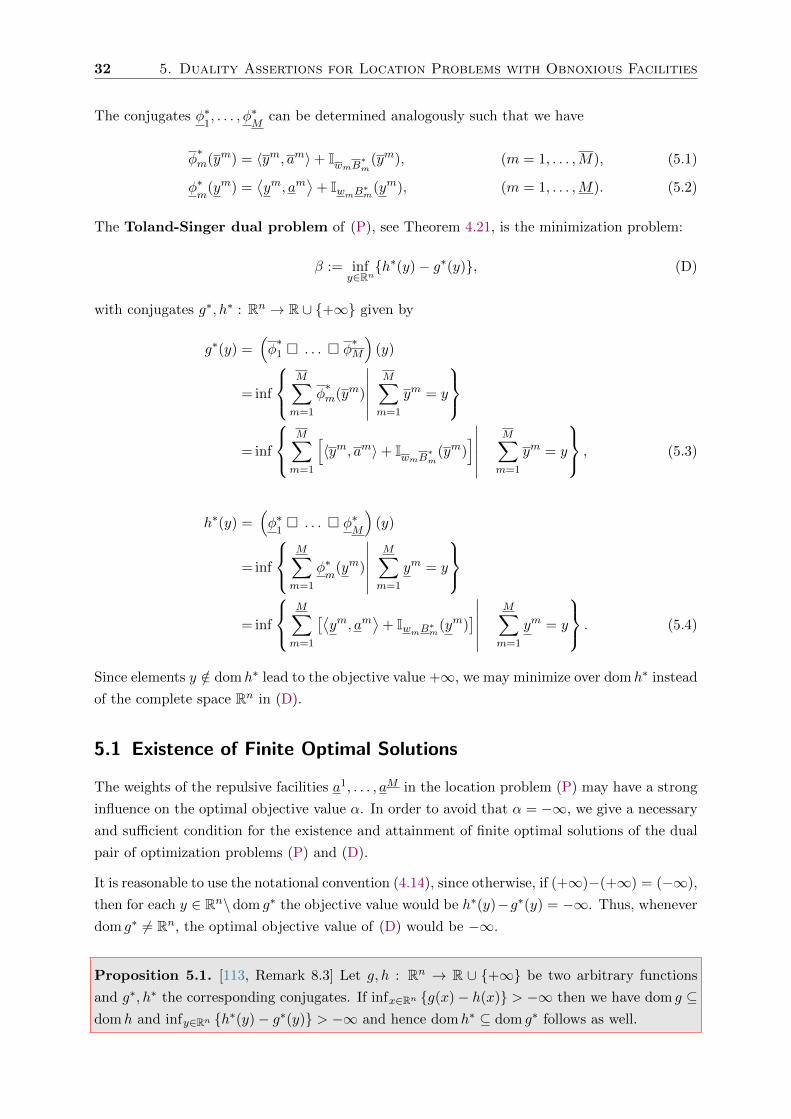
32 5. Duality Assertions for Location Problems with Obnoxious Facilities
The conjugates φ∗1, . . . , φ∗
Mcan be determined analogously such that we have
φ∗m(ym) = 〈ym, am〉+ IwmB
∗m
(ym), (m = 1, . . . ,M), (5.1)
φ∗m
(ym) =⟨ym, am
⟩+ IwmB
∗m
(ym), (m = 1, . . . ,M). (5.2)
The Toland-Singer dual problem of (P), see Theorem 4.21, is the minimization problem:
β := infy∈Rn{h∗(y)− g∗(y)}, (D)
with conjugates g∗, h∗ : Rn → R ∪ {+∞} given by
g∗(y) =(φ∗1 � . . . � φ
∗M
)(y)
= inf
M∑m=1
φ∗m(ym)
∣∣∣∣∣∣M∑m=1
ym = y
= inf
M∑m=1
[〈ym, am〉+ IwmB
∗m
(ym)]∣∣∣∣∣∣
M∑m=1
ym = y
, (5.3)
h∗(y) =(φ∗1� . . . � φ∗
M
)(y)
= inf
M∑m=1
φ∗m
(ym)
∣∣∣∣∣∣M∑m=1
ym = y
= inf
M∑m=1
[⟨ym, am
⟩+ IwmB
∗m
(ym)]∣∣∣∣∣∣
M∑m=1
ym = y
. (5.4)
Since elements y /∈ domh∗ lead to the objective value +∞, we may minimize over domh∗ instead
of the complete space Rn in (D).
5.1 Existence of Finite Optimal Solutions
The weights of the repulsive facilities a1, . . . , aM in the location problem (P) may have a strong
influence on the optimal objective value α. In order to avoid that α = −∞, we give a necessary
and sufficient condition for the existence and attainment of finite optimal solutions of the dual
pair of optimization problems (P) and (D).
It is reasonable to use the notational convention (4.14), since otherwise, if (+∞)−(+∞) = (−∞),
then for each y ∈ Rn\dom g∗ the objective value would be h∗(y)−g∗(y) = −∞. Thus, whenever
dom g∗ 6= Rn, the optimal objective value of (D) would be −∞.
Proposition 5.1. [113, Remark 8.3] Let g, h : Rn → R ∪ {+∞} be two arbitrary functions
and g∗, h∗ the corresponding conjugates. If infx∈Rn {g(x)− h(x)} > −∞ then we have dom g ⊆domh and infy∈Rn {h∗(y)− g∗(y)} > −∞ and hence domh∗ ⊆ dom g∗ follows as well.

5.1 Existence of Finite Optimal Solutions 33
By applying Proposition 5.1 we obtain the following necessary and sufficient condition for the
finiteness of the optimal objective values of the dual pair of optimization problems (P) and (D).
Theorem 5.2. (Finiteness Criterion)
The optimal objective value of the dual pair of optimization problems (P) and (D) is finite, i.e.,
infy∈Rn{h∗(y)− g∗(y)} = infx∈Rn {g(x)− h(x)} ∈ R, if and only if
M∑m=1
wmB∗m ⊆
M∑m=1
wmB∗m.
Proof. The function g∗, as given in (5.3), attains a finite objective value if and only if there
exists a tuple(y1, . . . , yM
)such that
∑Mm=1 y
m = y and ym ∈ wmB∗m for all m = 1, . . . ,M , i.e.,
g∗(y) ∈ R ⇔ y ∈M∑m=1
wmB∗m.
An analogous statement holds for h∗. Hence, the effective domains of h∗ and g∗ are given as
domh∗ =
M∑m=1
wmB∗m( 6= ∅) and dom g∗ =
M∑m=1
wmB∗m(6= ∅). (5.5)
From Proposition 5.1 we directly obtain
infy∈Rn{h∗(y)− g∗(y)} ∈ R ⇒
M∑m=1
wmB∗m ⊆
M∑m=1
wmB∗m.
Further, the objective value h∗(y)− g∗(y) is finite for all y ∈ domh∗ ∩ dom g∗. For y /∈ domh∗
we have by (4.14) that h∗(y)−g∗(y) = +∞, i.e., y does not contribute to the infimum of h∗−g∗
since domh∗ 6= ∅. Hence, we have
infy∈Rn{h∗(y)− g∗(y)} ∈ R ⇐
M∑m=1
wmB∗m ⊆
M∑m=1
wmB∗m
and the assertion holds.
By Theorem 5.2 we have found a necessary and sufficient condition for the finiteness of the
optimal objective values of the dual pair of optimization problems (P) and (D).
The effective domain of h∗, as the weighted sum of a finite number of convex, closed and bounded
balls B∗1, . . . , B∗M , is bounded and closed itself.
The function g∗, as the conjugate of the polyhedral function g, is polyhedral, too, and can be
decomposed as the sum of a piece-wise affine function g and the indicator function Idom g∗ , such
that g∗ = g + Idom g∗ , see Remark 4.6. Hence, we know from the Theorem by Weierstrass that

34 5. Duality Assertions for Location Problems with Obnoxious Facilities
g∗ attains a minimum and a maximum in dom g∗. Analogously, h∗ attains a minimum and a
maximum in domh∗.
Consequently, the objective function h∗ − g∗ (and hence the dual optimization problem (D))
attains a minimum in domh∗ ∩ dom g∗ and thus in domh∗ when domh∗ ⊆ dom g∗. Then also
the primal problem (P) does and we can substitute infimum by minimum in both problems.
Remark 5.3. In case that B1 = . . . = BM = B1 = . . . = BM in Theorem 5.2, the finite-
ness criterion for the dual pair of optimization problems (P) and (D) simplifies as follows:
infx∈Rn {g(x)− h(x)} = infy∈Rn{h∗(y)− g∗(y)} ∈ R, if and only if
M∑m=1
wm ≤M∑m=1
wm.
Hence, Theorem 5.2 is a generalization of Theorem 1 in [35] (see also [98, Theorem 2.3]).
In case that the optimal objective value is −∞ the problem (P) is already solved - the optimal
location of the new facility is infinitely far away. Since this is not applicable for practical
issues, one might either change some parameters (for instance the weights) or, alternatively,
some constraints might be considered, see Chapter 8. For example it seems to be reasonable to
require the new facility to be established within a given city or country.
Remark 5.4. Note that the dual feasible set domh∗ is bounded, whereas the primal feasible
set is unbounded. In Chapter 8 we will see that the boundedness into any direction of the primal
feasible set induces unboundedness into this direction within the dual feasible set.
5.2 Geometrical Properties, Duality Statements and Optimality
Conditions
In this section we present geometrical properties, duality results and optimality conditions for
the dual pair of optimization problems (P) and (D).
Proposition 5.5. For φ∗1, . . . , φ
∗M : Rn → R as given in (5.1), and φ∗
1, . . . , φ∗
M: Rn → R as
defined in (5.2) we have
∂φ∗m(ym) = am +NwmB
∗m
(ym), (m = 1, . . . ,M),
∂φ∗m
(ym) = am +NwmB∗m
(ym), (m = 1, . . . ,M).
Proof. From (5.1) we obtain for all m = 1, . . . ,M that
∂φ∗m(ym) = ∂
[〈ym, am〉+ IwmB
∗m
(ym)]. (5.6)

5.2 Geometrical Properties, Duality Statements and Optimality Conditions 35
Since the inner product 〈·, am〉 is continuous and convex on Rn and the indicator function IwmB∗m
is convex on Rn, we know from Theorem 4.9 that
∂[〈ym, am〉+ IwmB
∗m
(ym)]
= ∂ 〈ym, am〉+ ∂IwmB∗m
(ym). (5.7)
Further, by properties (E) and (J) in Section 4.2, it holds ∂ 〈ym, am〉 = {am} and
∂IwmB∗m
(ym) = NwmB∗m
(ym).
Thus, by (5.6) and (5.7), we have for all m = 1, . . . ,M
∂φ∗m(ym) = am +NwmB
∗m
(ym).
The second equality follows analogously, by taking into account (5.2).
Proposition 5.6. The subdifferentials ∂g∗(y) and ∂h∗(y) are non-empty for all y ∈ dom g∗ and
y ∈ domh∗, respectively.
Proof. The function g∗, as the conjugate of the polyhedral function g, is polyhedral, too, and can
be decomposed as the sum of a piece-wise affine function g and the indicator function Idom g∗ ,
such that g∗ = g + Idom g∗ , see Remark 4.6. By applying the sum rule for subdifferentials, see
Theorem 4.9, and property (J) in Section 4.2 we obtain for all y ∈ dom g∗
∂g∗(y) ⊇ ∂g(y) + ∂Idom g∗(y) = ∂g(y) +Ndom g∗(y),
which, obviously, is a non-empty set for all y ∈ dom g∗. Analogously, we obtain ∂h∗(y) 6= ∅ for
all y ∈ domh∗.
Theorem 5.7. For each tuple π = (y1, . . . , yM ) ∈ w1B∗1×· · ·×wMB
∗M the following statements
are equivalent:
1.⋂Mm=1
[am +NwmBm
(ym)]6= ∅,
2. g∗ is exact at y :=∑M
m=1 ym, i.e., g∗(y) =
∑Mm=1 〈am, ym〉,
3.⋂Mm=1
[am +NwmBm
(ym)]
= ∂g∗(∑M
m=1 ym).
Moreover, for each feasible y ∈ dom g∗ there exists a tuple π such that these statements hold.
Analogously, for each tuple π = (y1, . . . , yM ) ∈ w1B∗1 × · · · × wMB∗M the following statements
are equivalent:
1.⋂Mm=1
[am +NwmBm
(ym)]6= ∅,
2. h∗ is exact at y :=∑M
m=1 ym, i.e., h∗(y) =
∑Mm=1
⟨am, ym
⟩,

36 5. Duality Assertions for Location Problems with Obnoxious Facilities
3.⋂Mm=1
[am +NwmBm
(ym)]
= ∂h∗(∑M
m=1 ym)
.
Moreover, for each feasible y ∈ domh∗ there exists a tuple π such that these statements hold.
Proof. We prove the above statements only concerning the function g∗. The second part follows
analogously.
1. ⇒ 2. ⇒ 3.: By Proposition 5.5 we have
M⋂m=1
[am +NwmB
∗m
(ym)]
=M⋂m=1
∂φ∗m(ym)
and by (5.3) we have g∗ = φ1 � · · · � φM . The assertions follow directly from Theorem 4.16.
3. ⇒ 1.: For (y1, . . . , yM ) ∈ w1B∗1 × · · · × wMB
∗M it obviously follows from (5.5) that
y :=
M∑m=1
ym ∈M∑m=1
wmB∗m = dom g∗.
The assertion follows since ∂g∗(y) 6= ∅ for all y ∈ dom g∗, see Proposition 5.6.
The existence of such a tuple (y1, . . . , yM ) ∈ w1B∗1×· · ·×wMB
∗M follows from Theorem 4.15.
Proposition 5.8. For each x ∈ Rn the subdifferentials of g and h are given by
∂g(x) =
M∑m=1
argmaxy∈wmB
∗m
〈x− am, y〉 , ∂h(x) =
M∑m=1
argmaxy∈wmB
∗m
〈x− am, y〉 .
Proof. It holds by (3.1) and the sum rule for subdifferentials, see Theorem 4.9, that
∂g(x) = ∂M∑m=1
φm(x) =M∑m=1
∂φm(x)
for all x ∈ Rn. We show that
∂φm(x) = argmaxy∈wmB
∗m
〈x− am, y〉 , (m = 1, . . . ,M).

5.2 Geometrical Properties, Duality Statements and Optimality Conditions 37
Let x ∈ Rn. Then for all m = 1, . . . ,M we obtain the equivalences
ym ∈ ∂φm(x)⇔ x ∈ ∂φ∗m(ym) (5.8)
⇔ x ∈ am +NwmB∗m
(ym) (5.9)
⇔ x− am ∈ NwmB∗m
(ym)
⇔ ∀y ∈ wmB∗m : 〈x− am, y − ym〉 ≤ 0 and ym ∈ wmB
∗m (5.10)
⇔ ∀y ∈ wmB∗m : 〈x− am, y〉 ≤ 〈x− am, ym〉 and ym ∈ wmB
∗m
⇔ ym ∈ argmaxy∈wmB
∗m
〈x− am, y〉 .
Equivalence (5.8) holds by Proposition 4.12, and (5.9) holds by Proposition 5.5. Further, equiv-
alence (5.10) holds by definition of the normal cone, see (4.1); ym ∈ wmB∗m since otherwise
NwmB∗m
(ym) = ∅ in contradiction to x − am ∈ NwmB∗m
(ym). The proof of the second assertion
follows analogously.
Corollary 5.9. For x ∈ Rn and ym ∈ wmB∗m, m ∈
{1, . . . ,M
}, the following equivalence holds:
x ∈ am +NwmB∗m
(ym) ⇔ ym ∈ argmaxy∈wmB
∗m
〈x− am, y〉 ,
and analogously, for x ∈ Rn and ym ∈ wmB∗m, m ∈ {1, . . . ,M}, we have
x ∈ am +NwmB∗m
(ym) ⇔ ym ∈ argmaxy∈wmB
∗m
〈x− am, y〉 .
Proof. From Proposition 5.5 and Proposition 5.8 we have
∂φ∗m(ym) = am +NwmB
∗m
(ym), ∂φm(x) = argmaxy∈wmB
∗m
〈x− am, y〉 .
The assertion follows by Proposition 4.12.
From Theorem 5.7 and Definition 4.17 we know that the elementary convex sets for the primal
problem (P) coincide with the subdifferentials of the conjugate functions g∗ and h∗. Analogously,
we define dual elementary convex sets using the subdifferentials of the functions g and h:
Definition 5.10. Consider the dual problem (D). For x ∈ Rn we call the sets
∂g(x) =M∑m=1
argmaxy∈wmB
∗m
〈x− am, y〉 and ∂h(x) =
M∑m=1
argmaxy∈wmB
∗m
〈x− am, y〉
dual elementary convex set w.r.t. attraction and w.r.t. repulsion, respectively.

38 5. Duality Assertions for Location Problems with Obnoxious Facilities
The corresponding dual (construction) grids are given by
GD :=⋃
{x∈Rn| dim ∂g(x)=1}
∂g(x) and GD :=⋃
{x∈Rn| dim ∂h(x)=1}
∂h(x).
A point y ∈ Rn is called dual grid point (also dual intersection point) w.r.t. attraction (repulsion),
if y is an extreme point of an elementary convex set w.r.t. attraction (resp. repulsion). We denote
by ID and ID the sets of all grid points w.r.t. attraction and w.r.t. repulsion, respectively.
Remark 5.11. Obviously, the definition of the sets of dual grid points w.r.t. attraction and
w.r.t. repulsion, as given in Definition 5.10, is equivalent to the following:
ID :=⋃
{x∈Rn|dim ∂g(x)=0}
∂g(x) = {y ∈ dom g∗| ∃x ∈ Rn : {y} = ∂g(x)} ,
ID :=⋃
{x∈Rn| dim ∂h(x)=0}
∂h(x) = {y ∈ domh∗| ∃x ∈ Rn : {y} = ∂h(x)} .
Figure 5.1 illustrates for Example 4.18 the effective domains dom g∗ and domh∗ as well as the
dual construction grids GD with respect to attraction (green grids) and GD with respect to
repulsion (red grids) for different choices of attraction and repulsion weights. The shape of the
dual elementary convex sets is similar in each picture and differs only depending on the weights.
In Figures 5.1c and 5.1i the finiteness criterion, given in Theorem (5.2), is not satisfied since,
obviously, domh∗ 6⊆ dom g∗.
In Figure 5.1d it holds that ∂h(x) ⊆ g(x) is true, if and only if x = a2, where
ext(∂g(a2)
)={
(−1,−2)T , (3,−2)T , (−1, 2)T , (3, 2)T}.
Hence, by Theorem 4.22, the only primal element that may be optimal for (P) is x = a2.
The relationship between primal and dual elementary convex sets is further described by an
inclusion-reversion one-to-one map in Chapter 6.

5.2 Geometrical Properties, Duality Statements and Optimality Conditions 39
(a) w1 = w2 = 1; w1 = 0.5 (b) w1 = w2 = 1 (c) w1 = w2 = 1; w1 = 1.5
(d) w1 = 1; w2 = 2; w1 = 0.5 (e) w1 = 1; w2 = 2; w1 = 1 (f) w1 = 1; w2 = 2; w1 = 1.5
(g) w1 = 2; w2 = 1; w1 = 0.5 (h) w1 = 2; w2 = 1; w1 = 1 (i) w1 = 2; w2 = 1; w1 = 1.5
Figure 5.1: The effective domains of g∗ and h∗ as well as the dual construction grids GD with respectto attraction (green grids) and GD with respect to repulsion (red grids) for different choicesof weights.
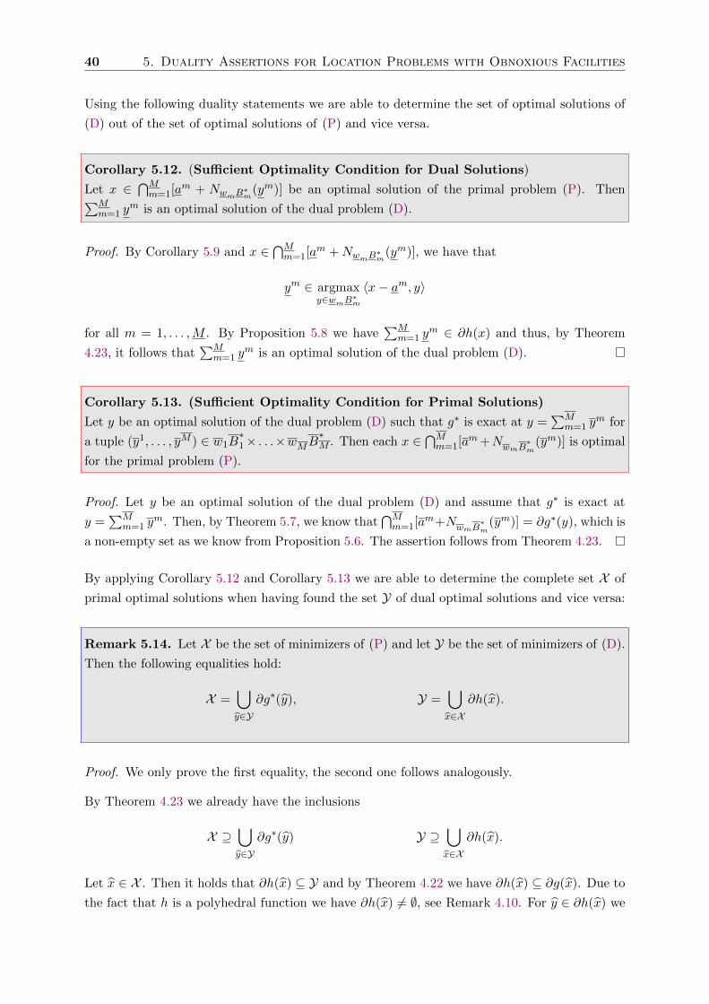
40 5. Duality Assertions for Location Problems with Obnoxious Facilities
Using the following duality statements we are able to determine the set of optimal solutions of
(D) out of the set of optimal solutions of (P) and vice versa.
Corollary 5.12. (Sufficient Optimality Condition for Dual Solutions)
Let x ∈⋂Mm=1[a
m + NwmB∗m
(ym)] be an optimal solution of the primal problem (P). Then∑Mm=1 y
m is an optimal solution of the dual problem (D).
Proof. By Corollary 5.9 and x ∈⋂Mm=1[a
m +NwmB∗m
(ym)], we have that
ym ∈ argmaxy∈wmB
∗m
〈x− am, y〉
for all m = 1, . . . ,M . By Proposition 5.8 we have∑M
m=1 ym ∈ ∂h(x) and thus, by Theorem
4.23, it follows that∑M
m=1 ym is an optimal solution of the dual problem (D).
Corollary 5.13. (Sufficient Optimality Condition for Primal Solutions)
Let y be an optimal solution of the dual problem (D) such that g∗ is exact at y =∑M
m=1 ym for
a tuple (y1, . . . , yM ) ∈ w1B∗1× . . .×wMB
∗M . Then each x ∈
⋂Mm=1[a
m+NwmB∗m
(ym)] is optimal
for the primal problem (P).
Proof. Let y be an optimal solution of the dual problem (D) and assume that g∗ is exact at
y =∑M
m=1 ym. Then, by Theorem 5.7, we know that
⋂Mm=1[a
m+NwmB∗m
(ym)] = ∂g∗(y), which is
a non-empty set as we know from Proposition 5.6. The assertion follows from Theorem 4.23.
By applying Corollary 5.12 and Corollary 5.13 we are able to determine the complete set X of
primal optimal solutions when having found the set Y of dual optimal solutions and vice versa:
Remark 5.14. Let X be the set of minimizers of (P) and let Y be the set of minimizers of (D).
Then the following equalities hold:
X =⋃y∈Y
∂g∗(y), Y =⋃x∈X
∂h(x).
Proof. We only prove the first equality, the second one follows analogously.
By Theorem 4.23 we already have the inclusions
X ⊇⋃y∈Y
∂g∗(y) Y ⊇⋃x∈X
∂h(x).
Let x ∈ X . Then it holds that ∂h(x) ⊆ Y and by Theorem 4.22 we have ∂h(x) ⊆ ∂g(x). Due to
the fact that h is a polyhedral function we have ∂h(x) 6= ∅, see Remark 4.10. For y ∈ ∂h(x) we
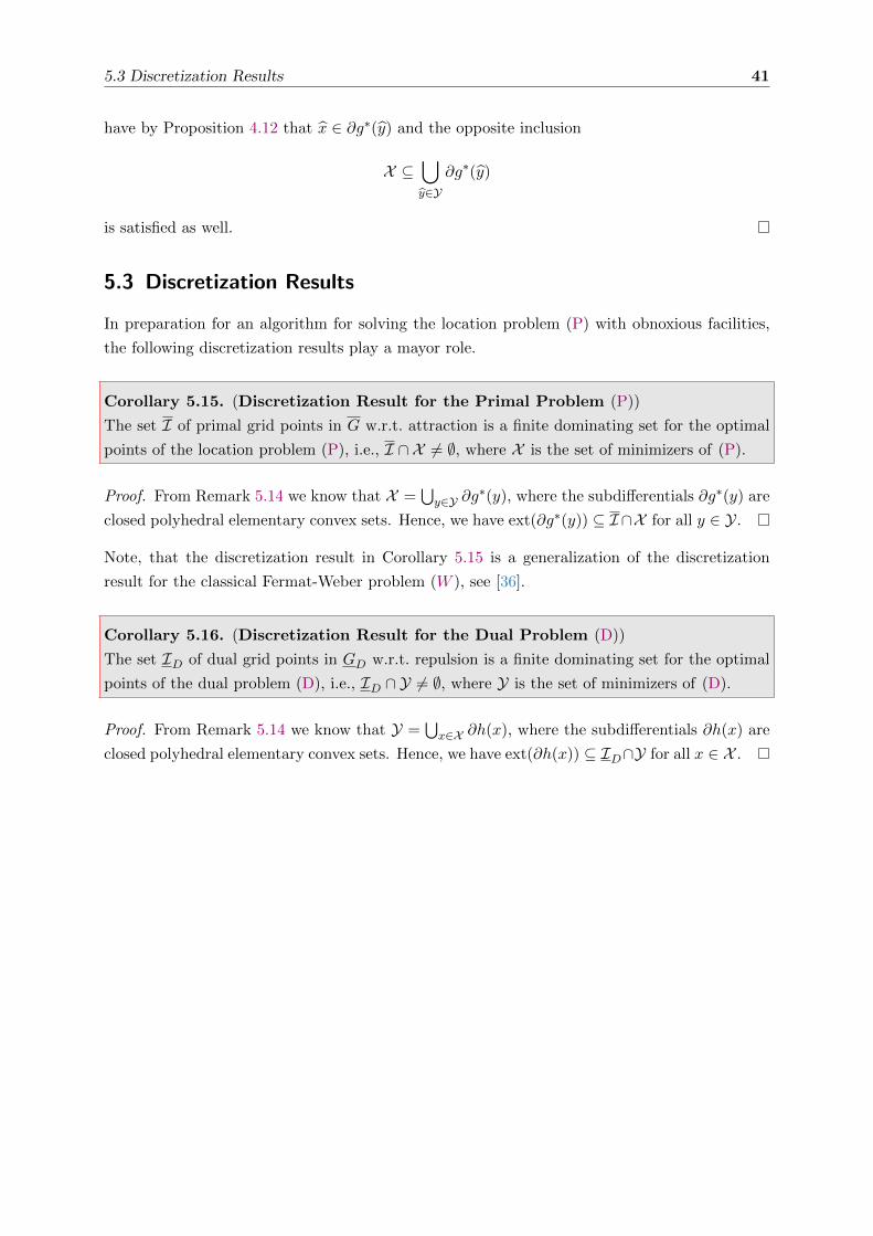
5.3 Discretization Results 41
have by Proposition 4.12 that x ∈ ∂g∗(y) and the opposite inclusion
X ⊆⋃y∈Y
∂g∗(y)
is satisfied as well.
5.3 Discretization Results
In preparation for an algorithm for solving the location problem (P) with obnoxious facilities,
the following discretization results play a mayor role.
Corollary 5.15. (Discretization Result for the Primal Problem (P))
The set I of primal grid points in G w.r.t. attraction is a finite dominating set for the optimal
points of the location problem (P), i.e., I ∩ X 6= ∅, where X is the set of minimizers of (P).
Proof. From Remark 5.14 we know that X =⋃y∈Y ∂g
∗(y), where the subdifferentials ∂g∗(y) are
closed polyhedral elementary convex sets. Hence, we have ext(∂g∗(y)) ⊆ I∩X for all y ∈ Y.
Note, that the discretization result in Corollary 5.15 is a generalization of the discretization
result for the classical Fermat-Weber problem (W ), see [36].
Corollary 5.16. (Discretization Result for the Dual Problem (D))
The set ID of dual grid points in GD w.r.t. repulsion is a finite dominating set for the optimal
points of the dual problem (D), i.e., ID ∩ Y 6= ∅, where Y is the set of minimizers of (D).
Proof. From Remark 5.14 we know that Y =⋃x∈X ∂h(x), where the subdifferentials ∂h(x) are
closed polyhedral elementary convex sets. Hence, we have ext(∂h(x)) ⊆ ID∩Y for all x ∈ X .


Chapter 6An Assignment between Primal and Dual
Elements Based on Geometric Duality
In this chapter, we apply results from the theory of geometric duality [56] in order to describe the
assignment between primal and dual elementary convex sets by an inclusion reversing one-to-one
mapping.
Consider the cone
K := {(x, r) ∈ Rn × R|x = 0, r ≥ 0} , (6.1)
and the epigraph of a proper closed convex function f : Rn → R∪ {+∞}. A proper face F , see
Definition 4.2, of epi f is called K-minimal if all of its points are minimal with respect to K,
i.e.,
∀y ∈ F : (y −K\(−K)) ∩ epi f = ∅. (6.2)
Proposition 6.1. [56, Proposition 3.2] A subset F ⊆ epi f is a K-minimal exposed face, see
Definition 4.2, of epi f if and only if there exists y ∈ dom f∗ with ∂f∗(y) 6= ∅ such that
F ={
(x, f(x)) ∈ Rn+1| y ∈ ∂f(x)}.
Further, a subset F ∗ ⊆ epi f∗ is a K-minimal exposed face of epi f∗ if and only if there exists
x ∈ dom f with ∂f(x) 6= ∅ such that
F ∗ ={
(y, f∗(y)) ∈ Rn+1| y ∈ ∂f(x)}.
The following theorem describes an assignment between K-minimal exposed faces F of epi f
and K-minimal exposed faces F ∗ of epi f∗.

44 6. An Assignment between Primal and Dual Elements
Theorem 6.2. (Geometric Duality Map for Epigraphs )
[56, Theorem 3.3] The mapping ψ : 2Rn+1 → 2R
n+1defined by
ψ(F ∗) :=⋂
(y,f∗(y))∈F ∗
{(x, f(x)) ∈ Rn+1| y ∈ ∂f(x)
}is an inclusion reversing one-to-one mapping (F ∗1 ⊆ F ∗2 if and only if ψ(F ∗1 ) ⊇ ψ(F ∗2 )) between
K-minimal exposed faces of epi f∗ and K-minimal exposed faces of epi f . Its inverse mapping
is given by
ψ∗(F ) :=⋂
(x,f(x))∈F
{(y, f∗(y)) ∈ Rn+1| y ∈ ∂f(x)
}.
Subsection 4.2 in [56] also provides the result
dimF ∗ + dimψ(F ∗) = n (6.3)
concerning the mapping ψ in Theorem 6.2.
Geometric Duality Map for Elementary Convex Sets
Since the function g, as given by (3.1) in the location problem (P), and its conjugate g∗, see
(5.3) in the dual problem (D), are polyhedral and convex, the epigraphs epi g ⊆ Rn+1 and
epi g∗ ⊆ Rn+1 are polyhedral and convex sets.
According to Proposition 6.1 each exposed K-minimal face F of epi g is given by a suitable
y ∈ dom g∗ as
F = {(x, g(x))| x ∈ ∂g∗(y)} =: F y
and each exposed K-minimal face F∗
of epi g∗ is given by a suitable x ∈ dom g as
F∗
= {(y, g∗(y))| y ∈ ∂g(x)} =: F∗x.
According to Theorem 6.2 and Equation (6.3) the map ψ∗
: 2Rn+1 → 2R
n+1defined by
ψ∗(F ) =
⋂(x,g(x))∈F
F∗x
provides an inclusion-reversing one-to-one map between the K-minimal faces of epi g and epi g∗
such that
dimF + dimψ∗(F ) = n.

45
Remark 6.3. The projection of an exposed face F y = {(x, g(x))| x ∈ ∂g∗(y)} ⊆ epi g onto Rn
obviously coincides with the elementary convex set ∂g∗(y), and the projection of an exposed face
F∗x = {(y, g∗(y))| y ∈ ∂g(x)} ⊆ epi g∗ onto Rn coincides with the elementary convex set ∂g(x).
On the other hand, the elementary convex sets ∂g∗(y) and ∂g(x) generate the exposed faces
F y = {(x, g(x))| x ∈ ∂g∗(y)} and F∗x = {(y, g∗(y))| y ∈ ∂g(x)} ,
i.e., there is a one-to-one relationship between the K-minimal faces F y of epi g and F∗x of epi g∗
and the elementary convex sets ∂g∗(y) and ∂g(x), respectively, such that
(x, g(x)) ∈ F y ⇔ x ∈ ∂g∗(y), dimF y = dim ∂g∗(y),
(y, g∗(y)) ∈ F ∗x ⇔ y ∈ ∂g(x), dimF∗x = dim ∂g(x).
Consequently the following duality result holds:
Theorem 6.4. (Assignment between Primal and Dual Elementary Convex Sets)
Let C := {∂g∗(y)| y ∈ dom g∗} ⊆ 2Rn
and D := {∂g(x)|x ∈ Rn} ⊆ 2Rn. The function Ψ
∗: C→
D, defined by
Ψ∗(∂g∗(y)) :=
⋂x∈∂g∗(y)
∂g(x),
provides an inclusion-reversing one-to-one map between the primal and dual elementary convex
sets, such that
dim ∂g∗(y) + dim Ψ∗(∂g∗(y)) = n.
Note that the results of this chapter hold analogously for the epigraphs of h and h∗ and the
corresponding primal and dual elementary convex sets w.r.t. repulsion.
Example
The assignment between primal and dual elementary convex sets in case of the 2-dimensional
space R2 is illustrated in Figure 6.1. The figure refers to the attracting points of Example 4.18
with weights w1 = 2 and w2 = 1 and illustrates the primal and the dual construction grids G
and GD w.r.t. attraction. The sum of the dimensions of each dual pair of assigned elementary
convex sets is dim ∂g∗(y) + dim Ψ(∂g∗(y)) = 2.
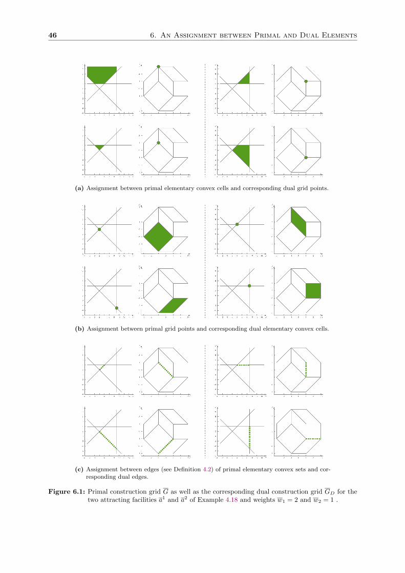
46 6. An Assignment between Primal and Dual Elements
(a) Assignment between primal elementary convex cells and corresponding dual grid points.
(b) Assignment between primal grid points and corresponding dual elementary convex cells.
(c) Assignment between edges (see Definition 4.2) of primal elementary convex sets and cor-responding dual edges.
Figure 6.1: Primal construction grid G as well as the corresponding dual construction grid GD for thetwo attracting facilities a1 and a2 of Example 4.18 and weights w1 = 2 and w2 = 1 .
Chapter 7An Application of Benson’s Algorithm for
Solving the Scalar Location Problem (P)
Although, we are considering a scalar optimization problem, we show in this chapter that meth-
ods from the field of linear vector optimization, in particular the well known Benson algorithm
[5, 76, 51], can be applied in order to determine the primal and dual grid points with respect to
attraction and to repulsion, as introduced in Definitions 4.17 and 5.10. Based on the discretiza-
tion results presented in Section 5.3, those grid points play a role in Chapter 9 for deriving an
algorithm for solving the location problem (P) with obnoxious facilities.
Let C ⊆ Rq be a polyhedral cone with non-empty interior, which does not contain any line.
Consider the linear vector optimization problem
C −minPx, P ∈ Rq×n, (LVOP)
subject to the set S := {x ∈ Rn|Bx ≥ b}, B ∈ Rm×n, b ∈ Rm. The set P := P [S] + C is called
upper image of (LVOP). A point x ∈ S is called a minimizer of (LVOP), if
P [S] ∩ (Px− C\ {0}) = ∅.
The geometric dual problem [51] is
K −maxD∗(u, η), (LVOD)
with respect to the cone K, given in (6.1), the linear objective function D∗ : Rm × Rq → Rq
defined by
D∗(u, η) := (η1, . . . , ηq−1, 〈b, u〉),
and the feasible set
T :={
(u, η) ∈ Rm+ × Rq∣∣BTu = P T η, 〈c, η〉 = 1, Y T η ≥ 0
}, (7.1)
48 7. An Application of Benson’s Algorithm
where Y is a matrix whose columns are generators of the ordering cone C and c ∈ Rq is a vector
contained in the interior of C with positive last entry. The set D∗ := D∗[T ]−K is called lower
image of (LVOD). A pair (u, η) ∈ T is called a maximizer of (LVOD), if
D∗[T ] ∩ (D∗(u, η) +K\ {0}) = ∅.
To solve such a linear vector optimization problem (LVOP) one can use the well known Benson
algorithm [5]. The extended version of Benson’s algorithm, presented in [51], solves the linear
vector optimization problem (LVOP) and its geometric dual problem (LVOD) by determining an
inequality representation as well as the extreme points and extreme directions of the polyhedral
sets P [S] + C and D∗[T ]−K with P , S, C and D∗, T , K as given above.
A Primal Linear Vector Optimization Problem Related to Repulsion
In order to apply Benson’s method, we show in the following, that the epigraph of h, where
h(x) =∑M
m=1wmγBm(x − am), as defined by (3.2) in the location problem (P), coincides with
the upper image of a linear vector optimization problem related to repulsion.
We use a ”primal” representation of the epigraph of h, ”primal” in the sense that this represen-
tation is based on the primal unit balls B1, . . . BM :
epih
=
(x, t) ∈ Rn+1
∣∣∣∣∣∣ t ≥ h(x) =
M∑m=1
wmγBm(x− am)
=
(x, t) ∈ Rn+1
∣∣∣∣∣∣ t ≥M∑m=1
wm min {λ ≥ 0| (x− am) ∈ λBm}
=
(x, t) ∈ Rn+1
∣∣∣∣∣∣ ∃λ1, . . . , λM ≥ 0 : ∀m = 1, . . . ,M : (x− am) ∈ λmBm, t ≥M∑m=1
wmλm,
.
Further, we define the feasible set
S :={(x, (λ1, . . . , λM ), t
)∈ Rn × RM × R
∣∣λ1, . . . , λM ≥ 0, ∀m = 1, . . . ,M : (x− am) ∈ λmBm, t ≥
M∑m=1
wmλm,
. (7.2)
In the following we denote by En the identity matrix in Rn and by 0n,M , 0n,1, 01,M , 01,n the
zero matrices in the dimensions defined by their indices. Writing the unit balls B1, . . . , BM as
Bm = {x ∈ Rn| Amx ≤ bm} , Am ∈ Rrm×n, bm ∈ Rrm , (m = 1, . . . ,M), (7.3)
49
and the constraints of the feasible set S in (7.2) into a common system of inequalities, we obtain
S ={z =
(x, (λ1, . . . , λM ), t
)∈ Rn × RM × R
∣∣Bz ≥ b}with
B :=
01,n 1 0 0...
. . ....
01,n 0 1 0
01,n −w1 · · · −wM 1
−A1 b1 0 0...
. . ....
−AM 0 bM 0
, b :=
0...
0
0
−A1 · a1...
−AM · aM
. (7.4)
The linear vector optimization problem related to repulsion can be formulated as
C −minx∈S
Px, (LVOP)
with suitable matrix P : Rn+M+1 → Rn+1 defined as
P :=
(En 0n,M 0n,1
01,n 01,M 1
),
and ordering cone C, which is chosen as the recession cone of the epigraph of h, i.e., C := 0+ epih.
Hence, by (4.2) and due to 0 ∈ 0+ epih, we obtain for the upper image of (LVOP)
P [S] + C = epih+ 0+ epih = epih.
The recession cone C = 0+ epih is determined below.
Analogously, for the function g, as defined by (3.1) in the location problem (P), we can define
a linear vector optimization problem related to attraction
C −minx∈S
Px, (LV OP )
with suitable matrix P ∈ R(n+1)×(n+M+1), feasible set S ⊆ Rn+M+1 and ordering cone C :=
0+ epi g, such that P [S] + C = epi g.
Determination of the Cones C and C
In order to determine the recession cone C = 0+ epih, we use a ”dual” representation of the
epigraph, ”dual” in the sense that this representation is based on the dual unit balls B∗1, . . . , B∗M .

50 7. An Application of Benson’s Algorithm
By (4.9) it holds
epih
=
(x, t) ∈ Rn+1
∣∣∣∣∣∣ t ≥ h(x) =
M∑m=1
wmγBm(x− am) =
M∑m=1
maxym∈ext(wmB
∗m)
⟨x− am, ym
⟩=
(x, t) ∈ Rn+1
∣∣∣∣∣∣ ∀(y1, . . . , yM ) ∈ ext(w1B∗1)× · · · × ext(wMB
∗M ) :
M∑m=1
⟨am, ym
⟩≥
M∑m=1
⟨x, ym
⟩− t
.
By applying Proposition 4.4 we obtain for the recession cone
C = 0+ epih
=
(x, t) ∈ Rn+1
∣∣∣∣∣∣∀(y1, . . . , yM ) ∈ ext(w1B∗1)× · · · × ext(wMB
∗M ) : 0 ≥
M∑m=1
⟨x, ym
⟩− t
=
(x, t) ∈ Rn+1
∣∣∣∣∣∣ t ≥M∑m=1
maxym∈wmB
∗m
⟨x, ym
⟩=
(x, t) ∈ Rn+1
∣∣∣∣∣∣ t ≥M∑m=1
wmγBm(x)
. (7.5)
The matrix Y , whose columns are the generators of the ordering cone C, contains as columns
the vectors d, M∑m=1
wmγBm(d)
∈ Rn+1,
for which d is a fundamental direction of at least one of the unit balls B1, . . . , BM .
Analogously, the recession cone C = O+ epi g can be written as
C = 0+ epi g =
(x, t) ∈ Rn+1
∣∣∣∣∣∣ t ≥M∑m=1
wmγBm(x)
,
and the matrix Y , whose columns are the generators of C, contains as columns the vectorsd, M∑m=1
wmγBm(d)
∈ Rn+1,
for which d is a fundamental direction of at least one of the unit balls B1, . . . , BM .

51
A Dual Linear Vector Optimization Problem Related to Repulsion
In the following we show that the epigraph of the function h∗ corresponds to the lower image of
the dual linear vector optimization problem related to repulsion.
Taking into account B, b, P , C, S, as defined in the primal linear vector optimization problem
(LVOP), as well as the cone K, as defined in (6.1), a geometric dual vector optimization
problem related to repulsion is given by
K − max(u,η)∈T
D∗(u, η), (LVOD)
with objective function
D∗(u, η) : = (η1, . . . , ηn, 〈b, u〉) (7.6)
and feasible set
T := {(u, η)| (i)-(vi) are satisfied} , (7.7)
where
(i) u = (u1, . . . , uM , v, z1, . . . , zM ) with (u1, . . . , uM ) ∈ RM+ , v ∈ R+ and zm ∈ Rrm+ for
m = 1, . . . ,M , where rm is the number of constraints, which define the unit ball Bm, see
(7.3),
η ∈ Rn+1, y := −(η1, . . . , ηn),
(ii) ηn+1 = 1,
(iii) v = 1,
(iv) y =∑M
m=1ATmz
m,
(v) um = wm − 〈bm, zm〉 for all m = 1, . . . ,M ,
(vi) For all (x, t) ∈ C it holds 〈x, y〉 ≤ t.
Proposition 7.1. Set c := (0, . . . , 0, 1) ∈ Rn+1. Then the set T has the structure as given in
(7.1), i.e., the following equivalences hold:
1. (ii) is equivalent to 〈c, η〉 = 1.
2. (iii), (iv) and (v) are equivalent to BTu = P T η.
3. (vi) holds if and only if Y T η ≥ 0, where Y is a matrix, whose columns generate the ordering
cone C.
52 7. An Application of Benson’s Algorithm
Proof.
1. For c := (0, . . . , 0, 1) ∈ Rn+1 we obtain 〈c, η〉 = 1 if and only if ηn+1 = 1, which coincides
with property (ii).
2. We further have equivalence between properties (iii), (iv) and (v) and BTu = P T η:
BTu =
−M∑m=1
ATmzm
u1 − w1 +⟨b1, z1
⟩...
uM − wM +⟨bM , zM
⟩1
=
−y0...
0
1
= P T η.
3. Let Y be a matrix, whose columns generate the ordering cone C. Then it holds Y T η ≥ 0
if and only if⟨(xt
), η⟩≥ 0 for all (x, t) ∈ C, where⟨(
x
t
), η
⟩=
⟨(x
t
),
(−y1
)⟩= −〈x, y〉+ t ≥ 0 ⇔ 〈x, y〉 ≤ t,
such that property (vi) is equivalent to Y T η ≥ 0.
Proposition 7.2. Let the properties (i) and (v) be satisfied, i.e., 〈bm, zm〉 ≤ wm and zm ≥ 0
for all m = 1, . . . ,M . Then it holds ATmzm ∈ wmB∗m for all m = 1, . . . ,M .
Proof. For all x ∈ Bm = {x ∈ Rn|Amx ≤ bm} we obtain
⟨x, ATmz
m⟩
= 〈Amx, zm〉 ≤ 〈bm, zm〉 ≤ wm.
The assertion follows since wmB∗m = {y ∈ Rn| ∀x ∈ Bm : 〈x, y〉 ≤ wm}, see (4.6).
Proposition 7.3. The properties (i), (iv) and (v) imply the property (vi).
Proof. Let (x, t) ∈ C and assume that z1, . . . , zM and y are given such that they satisfy the
properties (i), (iv) and (v). Then we obtain by (7.5), (4.9) and Proposition 7.2
t ≥M∑m=1
wmγBm(x) =
M∑m=1
maxym∈wmB
∗m
⟨x, ym
⟩≥
M∑m=1
⟨x,ATmz
m⟩
=
⟨x,
M∑m=1
ATmzm
⟩= 〈x, y〉 .

53
Proposition 7.4. For the lower image of the dual problem (LVOD) and the epigraph of h∗ it
holds
− (D∗[T ]−K) = epih∗.
Proof. For the dual objective function, as given in (7.6), we have by property (i) and by (7.4)
D∗(u, η) = (η1, . . . , ηn, 〈b, u〉) = −
y, M∑m=1
〈Amam, zm〉
= −
y, M∑m=1
⟨am, ATmz
m⟩ .
Taking into account the definition of the set T , see (7.7), and Proposition 7.3 we obtain
−D∗[T ] ={
(y, t) ∈ Rn+1∣∣∃z1, . . . , zM ≥ 0 :
∀m = 1, . . . ,M : 〈bm, zm〉 ≤ wm, y =
M∑m=1
ATmzm, t =
M∑m=1
⟨am, ATmz
m⟩ .
By definition of the ordering cone K, in (6.1), and Proposition 7.2 it follows
− (D∗[T ]−K)
=
(y, t) ∈ Rn+1
∣∣∣∣∣∣ ∃ (y1, . . . , yM) ∈ w1B∗1 × . . .× wMB∗M : y =
M∑m=1
ym, t ≥M∑m=1
⟨am, ym
⟩=
(y, t) ∈ Rn+1
∣∣∣∣∣∣ t ≥ inf
M∑m=1
⟨am, ym
⟩+ IwmB
∗m
(ym)
∣∣∣∣∣∣ y =
M∑m=1
ym
= h∗(y)
= epih∗,
and the assertion holds.
Analogously, we can define a geometric dual vector optimization problem related to
attraction
K − max(u,η)∈T
D∗(u, η), (LV OD)
with objective function D∗, dual feasible set T and ordering cone K, as given in (6.1), such that
epi g∗ = −(D∗[T ]−K
).

54 7. An Application of Benson’s Algorithm
Conclusion
We constructed a dual pair of linear vector optimization problems (LVOP) and (LVOD) such that
we obtain for the upper image P [S] +C = epih and for the lower image D∗[T ]−K = − epih∗.
Finding the exposed faces, see Definition 4.2, of epih and epih∗ means to minimize the linear
vector optimization problem (LVOP) and to maximize its geometric dual problem (LVOD). This
can be done by applying Benson’s algorithm. A numerical implementation of the primal and
dual variant of Benson’s algorithm, as presented in [51], is bensolve-1.2.1
The projections of the extreme points of epih and epih∗ onto Rn coincide with the primal and
dual grid points x ∈ I and y ∈ ID, w.r.t. repulsion, see Remark 6.3.
Based on the discretization results, presented in Section 5.3, those grid points play a role in
Chapter 9 for deriving an algorithm for solving the location problem (P) with obnoxious facilities.
Analogous results hold for the function g and its conjugate g∗.
1http://ito.mathematik.uni-halle.de/~loehne

Chapter 8Locating an Obnoxious Facility under
Consideration of Polyhedral Constraints
In practical applications it is reasonable to establish the new facility within a given area, a city
or a country for instance. Throughout this chapter we extend our research such that convex
polyhedral constraints are considered. We formulate a dual problem to the constrained location
problem, based on the duality theory by Toland [121] and Singer [112], see Theorem 4.21. In
Section 8.1 we provide some geometrical properties and duality statements. In Section 8.2 we
state a criterion for the finiteness of the objective value of such a constrained location problem.
In Section 8.3 we give optimality conditions and discretization results for both problems. Finally,
we illustrate the results of this chapter by some examples in Section 8.4.
Let H ⊆ Rn be given by the intersection of I closed half-spaces such that
H :=I⋂i=1
Hi, Hi :={x ∈ Rn|
⟨x, qi
⟩≤ ci
}, (i = 1, . . . , I), (8.1)
with qi ∈ Rn\ {0} and ci ∈ R, for i = 1, . . . , I. We assume that the half-spaces H1, . . . ,HI are
given such that their intersection H has non-empty interior and none of them is redundant, i.e.,
none of them can be omitted without changing the structure of H.
We consider the location problem with obnoxious facilities and convex constraints
minx∈H{g(x)− h(x)} , (8.2)
with
g(x) =
M∑m=1
wmγm(x− am), h(x) =
M∑m=1
wmγm(x− am).
as given by (3.1) and (3.2) in the location problem (P). Formulating (8.2) as an unconstrained

56 8. Consideration of Polyhedral Constraints
d.c. problem by using the indicator function, we obtain
αH : = minx∈Rn{gH(x)− h(x)}, (PH)
where gH(x) := g(x) + IH(x). Obviously, the constraints set H does not affect the function h.
Formulation of the Dual Problem
In order to formulate a Toland-Singer dual problem (DH) we determine the conjugate function
g∗H of the function gH.
Proposition 8.1. Let H( 6= ∅) ⊆ Rn be a convex set. Then the conjugate g∗H : Rn → R∪{+∞}is given by
g∗H(y) = infy0∈Rn
{g∗(y − y0) + σH(y0)
}= inf
M∑m=1
[〈am, ym〉+ IwmB
∗m
(ym)]
+ σH(y0)
∣∣∣∣∣∣M∑m=0
ym = y
.
with g∗ : Rn → R ∪ {+∞}, as given by (5.3) in (D).
Proof. The intersection int dom g ∩ int dom IH is non-empty since dom g = Rn and intH ⊆ Rn
is supposed to be non-empty. Further, the functions g and IH are convex. Hence, the assertion
follows by Theorem 4.15 and property (h) in Section 4.2:
g∗H(y) = (g + IH)∗(y) = (g∗ � I∗H) (y) = (g∗ � σH) (y) = infy0∈Rn
{g∗(y − y0) + σH(y0)
}.
Taking into account the structure of g∗, as given by (5.3) in (D), we obtain the more specific
formulation
g∗H(y) = (g + IH)∗(y)
=(φ1 + . . .+ φM + IH
)∗(y)
=(φ∗1 � . . . � φ
∗M � σH
)(y)
= inf
M∑m=1
[〈am, ym〉+ IwmB
∗m
(ym)]
+ σH(y0)
∣∣∣∣∣∣M∑m=0
ym = y
,
with φ1, . . . , φM as given by (3.1) in the location problem (P) and their conjugates φ∗1, . . . , φ
∗M
as given by (5.1) in the dual problem (D).
The Toland-Singer dual problem of (PH), see Theorem 4.21, is defined by
βH := infy∈Rn{h∗(y)− g∗H(y)} (DH)

8.1 Geometrical Properties 57
with conjugates h∗ : Rn → R ∪ {+∞}, as given by (5.4) in (D), and g∗H : Rn → R ∪ {+∞}, as
given by Proposition 8.1.
8.1 Geometrical Properties
In this section we provide some geometrical properties and duality statements of the dual pair
of optimization problems (PH) and (DH).
Proposition 8.2. Let H =⋂Ii=1Hi, Hi =
{x ∈ Rn|
⟨x, qi
⟩≤ ci
}with qi, ci, for i = 1, . . . , I, as
defined in (8.1). Moreover, define for x ∈ H the index set Jx :={i ∈ {1, . . . , I}
∣∣ ⟨x, qi⟩ = ci}
.
Then we have
∂gH(x) = ∂g(x) +NH(x), (8.3)
where
NH(x) =
∑i∈Jx
R+qi, if x ∈ bdH,
{0} , if x ∈ intH,
∅, if x /∈ H,
and ∂g(x) is given in Proposition 5.8.
Proof. Equation (8.3) follows from Theorem 4.9 and property (J) in Section 4.2:
∂gH(x) = ∂(g + IH)(x) = ∂g(x) + ∂IH(x) = ∂g(x) +NH(x).
From Theorem 4.9 and property (J) in Section 4.2 we obtain for x ∈ H
NH(x) = ∂IH(x) = ∂I∑i=1
IHi(x) =I∑i=1
∂IHi(x) =I∑i=1
NHi(x) =
∑
i∈Jx R+qi, x ∈ bdH,
{0} , x ∈ intH.
The last equation holds since NHi(x) = {0} for x ∈ intHi, i.e., whenever i /∈ Ix, and NHi(x) =
R+qi for x ∈ bdHi, i.e., whenever i ∈ Ix.
Proposition 8.3. The subdifferentials ∂g∗H(y), ∂gH(x) and ∂σH(y) are non-empty for all y ∈dom g∗H, x ∈ dom gH = H and y ∈ domσH, respectively.
Proof. The function IH is polyhedral, whenever H is a polyhedral set. Hence, the function
gH = g + IH and the conjugates I∗H = σH and g∗H are polyhedral, too. The assertions follow by
Remark 4.10.

58 8. Consideration of Polyhedral Constraints
Proposition 8.4. For H =⋂Ii=1Hi, Hi =
{x ∈ Rn|
⟨x, qi
⟩= ci
}with qi, ci (i = 1, . . . , I) as
defined in (8.1) the effective domain of σH is
domσH =I∑i=1
R+qi.
Proof. Let y ∈ domσH. Then by Proposition 8.3 and property (h) in Section 4.2 it holds
∂σH(y) = {x ∈ H|σH(y) = 〈x, y〉} 6= ∅.
By Proposition 4.12, properties (i) and (J) in Section 4.2 and Proposition 8.2 we have
x ∈ ∂σH(y) ⇔ y ∈ ∂σ∗H(x) = ∂IH(x) = NH(x) ⊆I∑i=1
R+qi.
Let y ∈∑I
i=1R+qi. Then there exist λ1, . . . , λI ≥ 0 such that y =
∑Ii=1 λiq
i. Hence, we obtain
σH(y) = supx∈H〈x, y〉 = sup
x∈H
⟨x,
I∑i=1
λiqi
⟩= sup
x∈H
I∑i=1
λi⟨x, qi
⟩≤
I∑i=1
λici < +∞,
i.e., y ∈ domσH.
Proposition 8.5. Let H =⋂Ii=1Hi, Hi =
{x ∈ Rn|
⟨x, qi
⟩≤ ci
}with qi, ci, for i = 1, . . . , I, as
defined in (8.1). Moreover, define for x ∈ H the index set Jx :={i ∈ {1, . . . , I}
∣∣ ⟨x, qi⟩ = ci}
.
Then for (y, y0) ∈ dom g∗H × domσH with y − y0 ∈ dom g∗ we have
∂g∗H(y) ⊇ ∂g∗(y − y0) ∩ ∂σH(y0), (8.4)
where
∂σH(y0) =
{x ∈ bdH
∣∣∣∣∣ y0 ∈∑i∈Ix
R+qi
}, if y0 ∈ domσH\ {0} ,
H, if y0 = 0,
∅, if y0 /∈ domσH,
and ∂g∗(y − y0) as given in Section 5.2.
Proof. Let (y, y0) ∈ dom g∗H×domσH such that y−y0 ∈ dom g∗ and ∂g∗(y−y0)∩∂σH(y0) 6= ∅.Then inclusion (8.4) holds by Theorem 4.16 and Proposition 8.1.
Let y0 = 0. Then, by property (H) in Section 4.2, it holds
∂σH(y0) ={x ∈ H
∣∣σH(y0) =⟨x, y0
⟩}= H.

8.2 Existence of Finite Optimal Solutions 59
Let y0 ∈ domσH\ {0}. By Remark 4.7, property (H) in Section 4.2 and Proposition 8.2 it follows
∂σH(y0) ={x ∈ H
∣∣σH(y0) =⟨x, y0
⟩}={x ∈ H
∣∣ y0 ∈ NH(x)}
=
{x ∈ bdH
∣∣∣∣∣ y0 ∈∑i∈Ix
R+qi
}.
Let y0 /∈ domσH, then ∂σH(y0) = ∅.
Theorem 8.6. For each pair (y, y0) ∈ dom g∗H × domσH with y − y0 ∈ dom g∗ the following
statements are equivalent:
1. ∂g∗(y − y0) ∩ ∂σH(y0) 6= ∅,
2. g∗H is exact at y := (y − y0) + y0,
3. ∂g∗(y − y0) ∩ ∂σH(y0) = ∂g∗H(y).
Moreover, for each feasible y ∈ dom g∗H there exists y0 ∈ domσH such that these statements
hold.
Proof. 1. ⇒ 2. ⇒ 3. Those implications follow directly by Theorem 4.16.
3. ⇒ 1. The assertion follows since ∂g∗H(y) 6= ∅ for all y ∈ dom g∗H, see Proposition 8.3.
The existence of such a pair (y, y0) ∈ dom g∗H × domσH follows from Theorem 4.15.
Corollary 8.7. If ∂g∗(y) ∩H 6= ∅, then it holds ∂g∗H(y) = ∂g∗(y) ∩H.
8.2 Existence of Finite Optimal Solutions
In general, constraints influence the finiteness of the optimal objective value of the location
problem. A necessary and sufficient criterion for the finiteness of the optimal objective value of
the dual pair of optimization problems (PH) and (DH), under consideration of the polyhedral
constraints as given in (8.1), is the following:
Theorem 8.8. (Finiteness Criterion)
The optimal objective value of the dual pair of optimization problems (PH) and (DH) is finite,
i.e., infx∈Rn {gH(x)− h(x)} = infy∈Rn {h∗(y)− g∗H(y)} ∈ R, if and only if
M∑m=1
wmB∗m ⊆
M∑m=1
wmB∗m +
I∑i=1
R+qi.
Proof. By Remark 4.14 and Proposition 8.1 we have dom g∗H = dom g∗ + domσH (6= ∅). Taking
into account the domains of g∗, h∗ and σH, as given in (5.5) and Proposition 8.4, the assertion
follows from Proposition 5.1 analogously as in Theorem 5.2.

60 8. Consideration of Polyhedral Constraints
Remark 8.9. In case of one half-space constraint, i.e., for H ={x ∈ Rn|
⟨x, q1
⟩= c1
}with
q1, c1 as defined in (8.1) it holds: If domh∗ and dom g∗ are symmetric with respect to the origin
then
domh∗ ⊆ dom g∗H ⇔ domh∗ ⊆ dom g∗.
If the number I of half-space constraints is greater than one, then the assertion may be wrong.
Proof. Let domh∗ ⊆ dom g∗H and y ∈ domh∗. Since domh∗ is symmetric we also have −y ∈domh∗ and y,−y ∈ dom g∗H.
Since dom g∗H = dom g∗ + domR+q1, there exist λ1, λ2 ≥ 0 such that
y − λ1q1 ∈ dom g∗, −y − λ2q1 ∈ dom g∗.
Due to the symmetry of dom g∗ we have
−y + λ1q1 ∈ dom g∗, y + λ2q
1 ∈ dom g∗.
Hence, the line segment [y−λ1q1, y+λ2q1] is a subset of the convex set dom g∗, and y ∈ dom g∗.
Let domh∗ ⊆ dom g∗. By 0 ∈ R+q1 it follows that dom g∗ ⊆ dom g∗H and the assertion holds.
If H is a bounded set the finiteness is even assured since then domσH = Rn and hence domh∗ ⊆dom g∗H = dom g∗ + domσH = Rn. An example is illustrated in Figure 8.1d in Section 8.4.
Moreover, the constraints Hi ={x ∈ Rn|
⟨qi, x
⟩≤ ci
}, for i = 1, . . . , I, in the constrained
location problem (PH), provoke into each direction q ∈∑I
i=1R+qi the boundedness of dom gH
and the unboundedness of dom g∗H.
8.3 Optimality Conditions and Discretization Results
Using the following duality statements we are able to determine the set of optimal solutions of
(DH) out of the set of optimal solutions of (PH) and vice versa.
Corollary 8.10. (Sufficient Optimality Condition for Dual Solutions)
Let x ∈⋂Mm=1[a
m + NwmB∗m
(ym)] be an optimal solution of the primal problem (PH). Then∑Mm=1 y
m is an optimal solution of the dual problem (DH).
Proof. This result follows analogously to Corollary 5.12, since the function h and its conjugate
h∗ are not influenced by the constraints H.
Corollary 8.11. (Sufficient Optimality Condition for Primal Solutions)
Let y be an optimal solution of the dual problem (DH) such that g∗H is exact at y = (y−y0)+y0,
(y− y0, y0) ∈ dom g∗ × domσH. Then each x ∈ ∂g∗(y− y0)∩ ∂σH(y0) is optimal for the primal
problem (PH).

8.3 Optimality Conditions and Discretization Results 61
Proof. Let y be an optimal solution of the dual problem (DH) and assume that g∗ is exact at
y = (y − y0) + y0. Then, by Theorem 8.6, we know that
∂g∗(y − y0) ∩ ∂σH(y0) = ∂g∗H(y),
which is a non-empty set by Proposition 8.3. The assertion follows by Remark 5.14.
By applying Remark 5.14, Corollary 8.10 and Corollary 8.11 we are able to determine the
complete set XH of primal optimal solutions when having found the set YH of dual optimal
solutions and vice versa.
Definition 8.12. For x ∈ H and y ∈ dom g∗H we call the subdifferentials ∂gH(x) and ∂g∗H(y)
primal and dual constrained elementary convex sets w.r.t. attraction. The primal and dual
constrained (construction) grids are defined by
GH
:=⋃
{y∈dom g∗H| dim ∂g∗H(y)=1}∂g∗H(y), G
HD :=
⋃{x∈H| dim ∂gH(x)=1}
∂gH(x).
A point x ∈ Rn is called primal constrained grid point w.r.t. attraction, if x is an extreme point
of a primal constrained elementary convex set w.r.t. attraction. We denote by IH the set of all
primal constrained grid points w.r.t. attraction.
A point y ∈ Rn is called dual constrained grid point w.r.t. attraction, if y is an extreme point of
a dual constrained elementary convex set w.r.t. attraction. We denote by IHD the set of all dual
constrained grid points w.r.t. attraction.
Note that primal and dual elementary convex sets w.r.t. repulsion in case of convex polyhedral
constraints coincide with the subdifferentials ∂h(x) and ∂h∗(y), as given in Section 5.2, since
the functions h and h∗ are not influenced by the constraints.
Theorem 8.13. (Geometric Duality Map for the Constrained Case))
Let CH := {∂g∗H(y)| y ∈ dom g∗H} ⊆ 2Rn
and DH := {∂gH(x)|x ∈ dom gH} ⊆ 2Rn. The function
Φ∗H : CH → DH defined by
Φ∗H(∂g∗H(y)) :=
⋂x∈∂g∗H(y)
∂gH(x)
provides an inclusion-reversing one-to-one map between the primal and dual elementary convex
sets such that
dim ∂g∗H(y) + dim Φ∗H(∂g∗H(y)) = n.
Proof. The assertion follows analogously as for Theorem 6.4 since gH : Rn → R is a polyhedral
convex function.

62 8. Consideration of Polyhedral Constraints
An example in R2 is illustrated in Figure 8.1, where dim ∂gH(x) + dim ∂g∗H(y) = 2 for each pair
of assigned elementary convex sets.
The discretization results for an unconstrained location problem (P) with obnoxious facilities,
given in Corollaries 5.15 and 5.16, can analogously be formulated for the more general case of a
constrained location problem (PH) with obnoxious facilities.
Corollary 8.14. (Discretization Result for the Primal Problem (PH))
The set IH of primal grid points in GH
w.r.t. attraction is a finite dominating set for the optimal
points of the location problem (PH), i.e., IH ∩ XH 6= ∅, where XH is the set of minimizers of
(PH).
Proof. By Remark 5.14 we have XH =⋃y∈YH ∂g
∗H(y), where the subdifferentials ∂g∗H(y) are
closed polyhedral elementary convex sets. Hence, we have ext(∂g∗H(y)) ⊆ IH ∩ XH for all
y ∈ YH.
Corollary 8.15. (Discretization Result for the Dual Problem (DH))
The set ID of all dual grid points in GD w.r.t. repulsion is a finite dominating set for the optimal
points of the dual problem (DH), i.e., ID ∩ YH 6= ∅, where YH is the set of minimizers of (D).
Proof. By Remark 5.14 we have YH =⋃x∈XH ∂h(x), where the subdifferentials ∂h(x) are closed
polyhedral elementary convex sets. Hence, we have ext(∂h(x)) ⊆ I ∩ YH for all x ∈ XH.
8.4 Example
In order to illustrate the influence of linear constraints we give some examples in R2. In Figure
8.1 we marked for Example 4.18 the different kinds of primal and dual elementary convex sets
∂g∗H(y) and ∂gH(x) by different colors and line styles. We distinguish the following categories
of elementary convex sets:
1. ∂g∗(y) ∩H 6= ∅, i.e., ∂g∗H(y) = ∂g∗(y) ∩H
a) If ∂g∗(y) ⊆ H, then the primal elementary convex set ∂g∗H(y) is not influenced by the
constraints set H, i.e., ∂g∗H(y) = ∂g∗(y).
i. dim ∂g∗(y) = 0 (green)
ii. dim ∂g∗(y) = 1 (some continuous lines)
iii. dim ∂g∗(y) = 2 (red).
b) If ∂g∗(y) 6⊆ H, then the primal elementary convex set ∂g∗H(y) is influenced by the
constraints set H, i.e., ∂g∗H(y) = ∂g∗(y) ∩H 6= ∂g∗(y).
i. dim ∂g∗(y) = 1 (some continuous lines)
ii. dim ∂g∗(y) = 2 (blue).

8.4 Example 63
2. ∂g∗(y) ∩H = ∅
a) dim ∂g∗H(y) = 0
i. ∂g∗H(y) ⊆ bdH ∩G (purple)
ii. ∂g∗H(y) ⊆ ext(H) (orange).
b) dim ∂g∗H(y) = 1
∂g∗H(y) ⊆ bdH (dashed lines).
The assigned dual elementary convex sets, see Theorem 8.13, are identified in the same manner
as their respective primal elementary convex sets.
.

64 8. Consideration of Polyhedral Constraints
(a) One single half-space constraint.
(b) Two parallel half-space constraints.
(c) Three half-space constraints.
(d) Bounded closed polyhedral constraints.
Figure 8.1: Primal and dual grids w.r.t. attraction forExample 4.18 under consideration of differ-ent polyhedral constraints.
H1 ={x ∈ Rn
∣∣∣ ⟨(−2, 5)T , x⟩ ≤ −4} ,domσH = R+
{(−2, 5)T
}.
H1 ={x ∈ R2
∣∣∣ ⟨(1, 0)T , x⟩ ≤ 5},
H2 ={x ∈ R2
∣∣∣ ⟨(−1, 0)T , x⟩ ≤ 1},
domσH = R× {0}.
H1 ={x ∈ R2
∣∣∣ ⟨(−3, 10)T , x⟩ ≤ −11} ,H2 =
{x ∈ R2
∣∣∣ ⟨(2, 4)T , x⟩ ≤ 18},
H3 ={x ∈ R2
∣∣∣ ⟨(3, 1)T , x⟩ ≤ 32},
domσH =
R+
{(−3, 10)T
}+ R+
{(2, 4)T
}+ R+
{(3, 1)T
}.
H1 ={x ∈ R2
∣∣∣ ⟨(−4, 7)T , x⟩ ≤ −10} ,H2 =
{x ∈ R2
∣∣∣ ⟨(0, 1)T , x⟩ ≤ 2},
H3 ={x ∈ R2
∣∣∣ ⟨(2, 1)T , x⟩ ≤ 24},
H4 ={x ∈ R2
∣∣∣ ⟨(1,−1)T , x⟩ ≤ 15},
H5 ={x ∈ R2
∣∣∣ ⟨(0,−1)T , x⟩ ≤ 4},
H6 ={x ∈ R2
∣∣∣ ⟨(−3,−1)T , x⟩ ≤ −2} ,domσH = R2.

Chapter 9An Algorithm for Solving Location Problems
with Obnoxious Facilities
In this chapter we formulate a primal and a dual algorithm for solving the problem of locating
an obnoxious facility.
In Sections 9.1 and 9.2 we present different methods for determining the sets I and ID of primal
grid points w.r.t. attraction and dual grid points w.r.t. repulsion. Based on the Corollaries 5.15
and 5.16, we use those grid points in Section 9.3 in order to formulate a primal and a dual
algorithm for solving the dual pair of optimization problems (P) and (D). The algorithms are
illustrated by an example in Section 9.4. Moreover, the special case of no repulsion is shortly
discussed in Section 9.5. Finally, algorithms for the more general case of the constrained location
problem (PH) and its dual problem (DH) are presented in Section 9.6.
9.1 Determination of Grid Points w.r.t. Attraction
In this section we present different methods for determining the set I of primal grid points
w.r.t. attraction. These grid points are determined in step 2 and used in in step 3 of the primal
Algorithm 9.2 for solving the optimization problem (P).
Application of Benson’s Algorithm for Determining I and ID
Although we are considering a scalar optimization problem it is possible to apply methods from
the field of linear vector optimization in order to determine the primal and dual grid points w.r.t.
attraction. In particular, we apply the well known Benson algorithm [5, 51, 76]. We consider the
objectives P ,D∗, feasible sets S, T and ordering cones C,K as introduced in Chapter 7. Then
the epigraphs of the functions g and g∗, as given by (3.1) and (5.3) in the location problem (P)
and its dual problem (D), can be written as
epi g = P [S] + C and epi g∗ = −(D∗[T ]−K
),

66 9. An Algorithm for Location Problems with Obnoxious Facilities
i.e., the upper and the lower image of the dual pair of linear vector optimization problems
C−minP [S], (LV OP )
K−maxD∗[T ]. (LV OD)
Minimizing the linear vector optimization problem (LV OP ) and maximizing its geometric dual
problem (LV OD) means to find the exposed faces, see Definition 4.2, and the extreme points
of epi g and epi g∗. The grid points x ∈ I and y ∈ ID then are given as the projections of those
extreme points onto Rn, see Remark 6.3, such that
I : ={x ∈ Rn
∣∣ (x, g(x)) ∈ ext(P [S] + C
)},
ID : ={y ∈ dom g∗
∣∣∣ (y, g∗(y)) ∈ ext(−(D
∗[T ]−K)
)}.
Note that the set of primal and dual grid points w.r.t. repulsion may be determined completely
analogously.
Determining I by Intersection of Fundamental Directions
The half-lines am +R+e for all e ∈ ext(Bm), m ∈{
1, . . . ,M}
, are called fundamental directions
and generate the primal grid w.r.t. attraction. The set I of grid points coincides with the set of
intersection points of all fundamental directions, such that
I :=⋃
(m1,m2)∈{1,...,M}2
{(am1 + R+e
1)∩(am2 + R+e
2)∣∣
(e1, e2) ∈ ext(Bm1)× ext(Bm2), e2 /∈ R+e1}.
Determining I in the Special Case of Manhattan Distances
In the special case that the assigned distance function for each attracting facility in the location
problem (P) is the Manhattan norm (4.3), i.e.,
B1 = . . . = BM = BManhattan =
{x ∈ Rn
∣∣∣∣∣n∑i=1
|xi| ≤ 1
},
we directly obtain the set I of primal grid points w.r.t. attraction as
I :={a11, . . . , a
M1
}× · · · ×
{a1n, . . . , a
Mn
}.
9.2 Determination of Grid Points w.r.t. Repulsion
In this section we present different methods for determining the dual grid points w.r.t. repulsion.
These grid points are determined in step 2 and used in in step 3 of the dual Algorithm 9.3 for
solving the dual pair of optimization problems (P) and (D).

9.2 Determination of Grid Points w.r.t. Repulsion 67
Application of Benson’s Algorithm for Determining I and ID
Consider the objectives P ,D∗, feasible sets S, T and ordering cones C,K as introduced in
Chapter 7. The epigraphs of the functions h and h∗, as given by (3.2) and (5.4) in the location
problem (P) and its dual problem (D), can be written as
epih = P [S] + C and epih∗ = − (D∗[T ]−K) ,
i.e., the upper and the lower image of a dual pair of linear vector optimization problems
C−minP [S], (LVOP)
K−maxD∗[T ]. (LVOD)
Minimizing the linear vector optimization problem (LVOP) and maximizing its geometric dual
problem LVOD means to find the exposed faces and the extreme points of epih and epih∗. The
grid points x ∈ I and y ∈ ID then are given as the projections of those extreme points onto Rn,
see Remark 6.3, such that
I : = {x ∈ Rn| (x, h(x)) ∈ ext (P [S] + C)} ,
ID : = {y ∈ domh∗| (y, h∗(y)) ∈ ext (−(D∗[T ]−K))} .
Determining ID in the Special Case of Manhattan Distances
Consider the special case that the corresponding distance function for each repulsive facility in
the location problem (P) is the Manhattan norm (4.3), i.e.,
B1 = . . . = BM = BManhattan =
{x ∈ Rn
∣∣∣∣∣n∑i=1
|xi| ≤ 1
}.
By Remark 5.11 the set ID of dual grid points w.r.t. repulsion is given by
ID = {y ∈ domh∗| ∃x ∈ Rn : {y} = ∂h(x)} .
Those dual elementary convex sets are defined (see Definition 5.10) by the subdifferentials
∂h(x) =
M∑m=1
argmaxym∈wmB
∗m
⟨x− am, ym
⟩.
In case of Manhattan distances the weighted dual unit balls wmB∗m can be written as
wmB∗m = [−wm, wm]× . . .× [−wm, wm] ⊆ Rn,
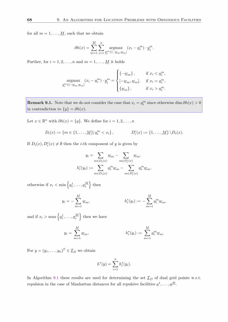
68 9. An Algorithm for Location Problems with Obnoxious Facilities
for all m = 1, . . . ,M , such that we obtain
∂h(x) =
M∑m=1
n∑i=1
argmaxymi∈[−wm,wm]
(xi − ami ) · ymi.
Further, for i = 1, 2, . . . , n and m = 1, . . . ,M it holds
argmaxymi∈[−wm,wm]
(xi − ami ) · ymi
=
{−wm} , if xi < ami ,
[−wm, wm], if xi = ami ,
{wm} , if xi > ami .
Remark 9.1. Note that we do not consider the case that xi = ami since otherwise dim ∂h(x) > 0
in contradiction to {y} = ∂h(x).
Let x ∈ Rn with ∂h(x) = {y}. We define for i = 1, 2, . . . , n
Di(x) := {m ∈ {1, . . . ,M}| ami < xi} , Dci (x) := {1, . . . ,M} \Di(x).
If Di(x), Dci (x) 6= ∅ then the i-th component of y is given by
yi =∑
m∈Di(x)
wm −∑
m∈Dci (x)
wm,
h∗i (yi) :=∑
m∈Di(x)
ami wm −∑
m∈Dci (x)
ami wm,
otherwise if xi < min{a1i , . . . , a
Mi
}then
yi = −M∑m=1
wm, h∗i (yi) := −M∑m=1
ami wm,
and if xi > max{a1i , . . . , a
Mi
}then we have
yi =
M∑m=1
wm, h∗i (yi) :=
M∑m=1
ami wm.
For y = (y1, . . . , yn)T ∈ ID we obtain
h∗(y) =n∑i=1
h∗i (yi).
In Algorithm 9.1 these results are used for determining the set ID of dual grid points w.r.t.
repulsion in the case of Manhattan distances for all repulsive facilities a1, . . . , aM .

9.2 Determination of Grid Points w.r.t. Repulsion 69
Algorithm 9.1 (Determination of dual set ID of grid points w.r.t. repulsion in Case of Man-
hattan Norm).
Input: am, wm, (m = 1, . . . ,M).
Output: ID, h∗[ID].
1. For i = 1, 2, . . . , n and m = 1, . . . ,M determine
Di(m) : ={m ∈ {1, . . . ,M}
∣∣∣ ami ≤ ami } , Dci (m) := {1, . . . ,M} \Di(m),
yi(0) : = −M∑m=1
wm,
yi(m) : =
∑m∈Di(m)
wm −∑
m∈Dci (m)
wm, if Dci (m) 6= ∅,
M∑m=1
wm, if Dci (m) = ∅,
h∗i (0) : = −M∑m=1
ami wm,
h∗i (m) : =
∑m∈Di(m)
ami wm −∑
m∈Dci (m)
ami wm, if Di(m), Dci (m) 6= ∅,
M∑m=1
ami wm, if Dci (m) = ∅.
2. Determine
ID =
M⋃m=0
{y1(m)} × . . .×M⋃m=0
{yn(m)} ⊆ Rn.
3. For each y := (y1(m1), . . . , yn(mn)) ∈ ID, with m1, . . . , mn ∈ {0, . . . ,M}, set
h∗(y) =n∑i=1
h∗i (mi).

70 9. An Algorithm for Location Problems with Obnoxious Facilities
Example 9.2. Suppose that we have given the repulsion points a1 = (1, 1), a2 = (2, 3), a3 =
(3, 2) and a4 = (2, 0) with corresponding weights w1 = 2, w2 = 1, w3 = 2 and w4 = 3. We
obtain
D1(1) = {1} , D2(1) = {1, 4} ,
D1(2) = {1, 2, 4} , D2(2) = {1, 2, 3, 4} ,
D1(3) = {1, 2, 3, 4} , D2(3) = {1, 3, 4} ,
D1(4) = {1, 2, 4} , D2(4) = {4} ,
y1(0) = −(w1 + w2 + w3 + w4) = −8, y2(0) = −(w1 + w2 + w3 + w4) = −8,
y1(1) = w1 − (w2 + w3 + w4) = −4, y2(1) = (w1 + w4)− (w2 + w3) = 2,
y1(2) = (w1 + w2 + w4)− w3 = 4, y2(2) = w1 + w2 + w3 + w4 = 8,
y1(3) = w1 + w2 + w3 + w4 = 8, y2(3) = (w1 + w3 + w4)− w2 = 6,
y1(4) = (w1 + w2 + w4)− w3 = 4, y2(4) = w4 − (w1 + w2 + w3) = −2,
and hence ID = {−8,−4, 4, 8} × {−8,−2, 2, 6, 8}.
Figure 9.1: Primal and dual grid w.r.t. repulsion in case of Manhattan distances.

9.3 Solving the Location Problem with Obnoxious Facilities 71
9.3 Solving the Location Problem with Obnoxious Facilities
Before starting the solving procedure, we apply Theorem 5.2 in step 1 of both, the primal
Algorithm 9.2 and the dual Algorithm 9.3, in order to check the finiteness of the optimal objective
value of the dual pair of optimization problems (P) and (D). In case of an infinite optimal
objective value, i.e., α = β := −∞, the algorithm quits. The primal set of optimal solutions is
X = ∅ and the dual set of optimal solutions is Y := domh∗\ dom g∗.
The Primal Algorithm
In case of a finite optimal objective value, one of the methods, presented in Section 9.1, is applied
in step 2 of Algorithm 9.2 for determining the set I of primal grid points w.r.t. attraction as
well as g[I]. In step 3, for each x ∈ I, the objective value h(x) is determined. Finally, in step
4, the primal minimal objective value
α := minx∈I{g(x− h(x)} ,
the primal set of optimal grid points
X := argminx∈I
{g(x)− h(x)} ,
and the dual set of optimal points
Y :=⋃x∈X
∂h(x) =⋃x∈X
M∑m=1
argmaxym∈ext(wmB
∗m)
⟨x− am, ym
⟩are determined, based on Corollary 5.12 and Proposition 5.8. By Theorem 4.21 the dual optimal
objective value β coincides with the primal one α.
The Dual Algorithm
In case of a finite optimal objective value, one of the methods presented in Section 9.2, is applied
in step 2 of Algorithm 9.3 for determining the set ID of dual grid points w.r.t. repulsion. In step
3, for each y ∈ ID the objective value g∗(y) is determined by solving the linear optimization
problem
g∗(y) = inf
M∑m=1
[〈am, ym〉+ IwmB
∗M
(ym)]∣∣∣∣∣∣
M∑m=1
ym = y
.
The tuples(y1, . . . , yM
), for which the infimum is attained, are used in step 4, where the dual
minimal objective value
β := miny∈ID
{h∗(y)− g∗(y)} ,

72 9. An Algorithm for Location Problems with Obnoxious Facilities
the dual set of optimal grid points
Y := argminy∈ID
{h∗(y)− g∗(y)} ,
and the primal set of optimal points
X :=⋃y∈Y
∂g∗(y) =⋃y∈Y
⋂m=1,...,M
[am +NwmB
∗m
(ym)],
are determined, based on Corollary 5.13 and Theorem 5.7. By Theorem 4.21 the primal optimal
objective value α coincides with the dual one β.
Algorithm 9.2 (Primal Algorithm for Solving the Location Problem (P)).
Input: am, wm, B∗m, (m = 1, . . . ,M); am, wm, B
∗m, (m = 1, . . . ,M).
Output: The sets X and Y of optimal grid points of (P) and (D); optimal objective value α.
1. Check finiteness of the optimal objective value using the condition
domh∗ =
M∑m=1
wmB∗m ⊆
M∑m=1
wmB∗m = dom g∗
given in Theorem 5.2. If the condition is satisfied go on with 2. Otherwise set α := −∞,
Y := domh∗\ dom g∗ and X := ∅ and STOP.
2. Determine the set I as well as g[I] by using one of the methods presented in Section 9.1.
3. For all x ∈ I determine h(x) :=∑M
m=1wmγBm(x− am).
4. Determine the optimal objective value
α := minx∈I{g(x)− h(x)} ,
the primal set of optimal grid points
X := argminx∈I
{g(x)− h(x)} ,
and the dual set of optimal points
Y :=⋃x∈X
∂h(x) =⋃x∈X
M∑m=1
argmaxym∈ext(wmB
∗m)
⟨x− am, ym
⟩.

9.3 Solving the Location Problem with Obnoxious Facilities 73
Algorithm 9.3 (Dual Algorithm for Solving the Location Problem (P)).
Input: am, wm, B∗m, (m = 1, . . . ,M); am, wm, B
∗m, (m = 1, . . . ,M).
Output: The sets X and Y of optimal grid points of (P) and (D); optimal objective value β.
1. Check finiteness of the optimal objective value using the condition
domh∗ =
M∑m=1
wmB∗m ⊆
M∑m=1
wmB∗m = dom g∗
given in Theorem 5.2. If the condition is satisfied go on with 2. Otherwise set β := −∞,
Y := domh∗\ dom g∗ and X := ∅ and STOP.
2. Determine the set ID and h∗[ID] by using one of the methods presented in Section 9.2.
3. For all y ∈ ID determine the objective value g∗(y) by solving the linear optimization
problem
g∗(y) = inf
M∑m=1
[〈am, ym〉+ IwmB
∗M
(ym)]∣∣∣∣∣∣
M∑m=1
ym = y
and determine the set Y of tuple (y1, . . . , yM ) for which the infimum is attained.
4. Determine the optimal objective value
β := miny∈ID
{h∗(y)− g∗(y)} ,
the dual set of optimal grid points
Y := argminy∈ID
{h∗(y)− g∗(y)} ,
and the primal set of optimal points
X :=⋃y∈Y
∂g∗(y) =⋃y∈Y
⋂m=1,...,M
[am +NwmB
∗m
(ym)].
Obviously, the time complexity of Algorithm 9.2 strongly depends on the number of primal
grid points w.r.t. attraction. The time complexity of Algorithm 9.3 strongly depends on the
number of dual grid points w.r.t. repulsion. For each grid point, a linear optimization problem
is to be solved in Algorithm 9.3. The complexity of each sub-problem depends on the number
of attraction points. In Section 10.4 we present some examples in order to demonstrate the
influence of the number of facilities (and hence grid points) on the running times.
Further considerations on duality based algorithms for practical usage, including results con-
cerning complexity and efficiency, will be presented in forthcoming studies.

74 9. An Algorithm for Location Problems with Obnoxious Facilities
9.4 Example
We consider again the location problem introduced in Example 4.18, i.e., we have two attraction
points a1 = (2, 2)T and a2 = (9, 4)T and one repulsion point a1 = (7, 1)T with assigned primal
and dual unit balls given by
ext(B1) ={±(1, 1)T ,±(1,−1)T
}, ext(B
∗1) =
{±(1, 0)T ,±(0, 1)T
},
ext(B2) ={±(1, 0)T ,±(0, 1)T
}, ext(B
∗2) =
{±(1, 1)T ,±(1,−1)T
},
ext(B1) ={
(−1, 0)T , (0, 1)T , (1,−1)T}, ext(B∗1) =
{(−1, 1)T , (−1,−2)T , (2, 1)T
}.
Moreover, we choose the weights such that w1 = w2 = w1 = 1.
Application of the Primal Algorithm
1. The finiteness criteria domh∗ ⊆ dom g∗ is satisfied since the effective domains of h∗ and
g∗ are given by
ext(domh∗) = ext
M∑m=1
wmB∗m
={
(−1, 1)T , (−1,−2)T , (2, 1)T},
ext(dom g∗) = ext
M∑m=1
wmB∗m
= [{−1, 1} × {−2, 2}] ∪ [{−2, 2} × {−1, 1}].
2. The primal grid points x ∈ I w.r.t. attraction and the corresponding objective values g(x)
are given by
x ∈ I (0, 4)T (2, 2)T (4, 4)T (9,−5)T (9, 4)T (9, 9)T
g(x) 11 9 7 16 7 12
where by (4.3) and (4.5)
g(x) = max{∣∣x1 − a11∣∣ , ∣∣x2 − a12∣∣}+
∣∣x1 − a21∣∣+∣∣x2 − a22∣∣ .
3. For each grid point x ∈ I we determine the corresponding objective value h(x) such that
x ∈ I (0, 4)T (2, 2)T (4, 4)T (9,−5)T (9, 4)T (9, 9)T
h(x) 10 6 6 10 7 12
where by (4.9)
h(x) = maxy∈B∗1
⟨x− a1, y
⟩.
The corresponding primal elementary convex sets ∂h(x) are illustrated in Figure 9.2.
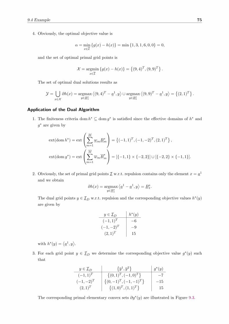
9.4 Example 75
4. Obviously, the optimal objective value is
α = minx∈I{g(x)− h(x)} = min {1, 3, 1, 6, 0, 0} = 0,
and the set of optimal primal grid points is
X = argminx∈I
{g(x)− h(x)} ={
(9, 4)T , (9, 9)T}.
The set of optimal dual solutions results as
Y =⋃x∈X
∂h(x) = argmaxy∈B∗1
⟨(9, 4)T − a1, y
⟩∪ argmax
y∈B∗1
⟨(9, 9)T − a1, y
⟩={
(2, 1)T}.
Application of the Dual Algorithm
1. The finiteness criteria domh∗ ⊆ dom g∗ is satisfied since the effective domains of h∗ and
g∗ are given by
ext(domh∗) = ext
M∑m=1
wmB∗m
={
(−1, 1)T , (−1,−2)T , (2, 1)T},
ext(dom g∗) = ext
M∑m=1
wmB∗m
= [{−1, 1} × {−2, 2}] ∪ [{−2, 2} × {−1, 1}].
2. Obviously, the set of primal grid points I w.r.t. repulsion contains only the element x = a1
and we obtain
∂h(x) = argmaxy∈B∗1
⟨a1 − a1, y
⟩= B∗1.
The dual grid points y ∈ ID w.r.t. repulsion and the corresponding objective values h∗(y)
are given by
y ∈ ID h∗(y)
(−1, 1)T −6
(−1,−2)T −9
(2, 1)T 15
with h∗(y) =⟨a1, y
⟩.
3. For each grid point y ∈ ID we determine the corresponding objective value g∗(y) such
that
y ∈ ID{y1, y2
}g∗(y)
(−1, 1)T{
(0, 1)T , (−1, 0)T}
−7
(−1,−2)T{
(0,−1)T , (−1,−1)T}
−15
(2, 1)T{
(1, 0)T , (1, 1)T}
15
The corresponding primal elementary convex sets ∂g∗(y) are illustrated in Figure 9.3.

76 9. An Algorithm for Location Problems with Obnoxious Facilities
4. Obviously, the optimal objective value is
α = miny∈ID
{h∗(y)− g∗(y)} = min {1, 6, 0} = 0,
and the set of optimal dual grid points is
Y = argminy∈ID
{h∗(y)− g∗(y)} ={
(2, 1)T}.
The set of optimal primal solutions results as
X =⋃y∈Y
∂g∗(y) = ∂g∗((2, 1)T ) = [a1 +NB∗1((1, 0)T )] ∩ [a2 +NB
∗2((1, 1)T )]
= [a1 + R+(1, 1)T + R+(1,−1)T ] ∩ [a2 + R2+].
Remark 9.3. Without solving the location problem, it is easy to see in Figure 9.2c that the
dual grid point y = (−1,−2)T can not be optimal for the dual problem (D), since the necessary
optimality condition ∂g∗(y) ⊆ ∂h∗(y), in Theorem 4.22, is not satisfied:
∂g∗((−1,−2)T ) = [a1 + R+(−1,−1)T + R+(1,−1)T ] ∩ [a2 − R2+],
∂h∗((−1,−2)T ) = [a1 + R+(−1, 0)T + R+(1,−1)T ].
Analogously, it is easy to see in Figure 9.2 that the primal grid point y = (2, 2)T can not be
optimal for the primal problem (P), since the necessary optimality condition ∂h(x) ⊆ ∂g(x), in
Theorem 4.22, is not satisfied:
ext(∂g((2, 2)T )) ={
(−2,−1)T ; (−1,−2)T ; (−1, 0)T ; (0,−1)T},
∂h((2, 2)T ) ={
(−1, 1)T}.

9.4 Example 77
(a) Primal and dual construction grids.
(b) x = (0, 4)T , x = (2, 2)T , x = (4, 4)T ; corresponding dual elementaryconvex set ∂h((0, 4)T ) = ∂h((2, 2)T ) = ∂h((4, 4)T ) =
{(−1, 1)T
}.
(c) x = (9,−5)T ; corresponding dual elementary convex set ∂h((9,−5)T ) ={(−1,−2)T
}.
(d) x = (9, 4)T , x = (9, 9)T ; corresponding dual elementary convex set∂h((9, 4)T ) = ∂h((9, 9)T ) =
{(2, 1)T
}.
Figure 9.2: Primal grid points x ∈ I (green) and the assigned dual elementary convex sets ∂h(x) (red)for the example in Section 9.4.

78 9. An Algorithm for Location Problems with Obnoxious Facilities
(a) Dual and primal construction grids.
(b) y = (−1, 1)T ; corresponding primal elementary convex set∂g∗((−1, 1)T ).
(c) y = (−1,−2)T ; corresponding primal elementary convex set∂g∗((−1,−2)T ).
(d) y = (2, 1)T ; corresponding primal elementary convex set ∂g∗((2, 1)T ).
Figure 9.3: Dual grid points y ∈ ID (red) and the assigned primal elementary convex sets ∂g∗(y) (green)for the example in Section 9.4.

9.5 The Special Case of no Repulsion 79
9.5 The Special Case of no Repulsion
For the classical Fermat-Weber problem (W ), as given in Section 4.3, the number of repulsion
points is equal to zero, i.e., M = 0. In this case the function h(x) does not contribute to the
objective function g(x)− h(x) in (P), in particular h ≡ 0. The conjugate h∗ then is given by
h∗(y) = supx∈Rn
{〈x, y〉 − 0} = I{0}(y)
and thus the effective domain results as domh∗ = {0} = ID = Y. Hence, the dual set of optimal
solutions is Y = {0}. The primal set of optimal points is given by X := ∂g∗(0), and the optimal
objective value α is finite. The dual problem (D) simplifies to
−g∗(0) = −min
M∑m=1
[〈am, ym〉+ IwmB
∗m
(ym)]∣∣∣∣∣∣
M∑m=1
ym = 0
,
and the dual algorithm reduces as follows:
Algorithm 9.4 (Dual algorithm in case of M = 0).
Input: am, wm, B∗m, (m = 1, . . . ,M).
Output: The set X of optimal grid points of of (PH); optimal objective value α.
Determine
α : = −min
M∑m=1
[〈am, ym〉+ IwmB
∗m
(ym)]∣∣∣∣∣∣
M∑m=1
ym = 0
,
X : =M⋂m=1
[am +NwmBm
(ym)].
In [36, Lemma 3.1] the authors give a statement on the existence of such a tuple of elements
y1, . . . , yM and a sufficient condition for a tuple to provide optimal solutions for this special case
of no repulsion. Nevertheless, we do not know from Lemma 3.1 in [36] how to determine such
a tuple. Using the duality based results of our study, we are able to determine such a tuple on
the one hand and also to generalize the assertion of Lemma 3.1 in [36] such, that an arbitrary
number of repulsion points may be considered, on the other hand.
9.6 An Algorithm for Solving the Constrained Problem with
Obnoxious Facilities
The Algorithms 9.2 and 9.3 can be generalized to the constrained case by substituting the
unconstrained function g and its conjugate g∗ by the constrained function gH and its conjugate

80 9. An Algorithm for Location Problems with Obnoxious Facilities
g∗H; and by taking into account the primal constrained set of grid points IH, see Definition
8.12. Note that the generalized Benson algorithm, as presented in [51], is not applicable for
determining the grid points x ∈ IH and y ∈ IHD, as described in Chapter 7 and Section 9.1.
In case of constraints the recession cone C := 0+ epi gH may have empty interior such that
the assumption c ∈ intC, see (7.1) in Chapter 7, is not satisfiable. A further generalization
of the algorithms is necessary to be able to deal with epigraphs of arbitrary polyhedral convex
functions, the development is in progress, see [77].
Algorithm 9.5 (Primal Algorithm for Solving the Constrained Location Problem (PH)).
Input: am, wm, B∗m, (m = 1, . . . ,M); am, wm, B
∗m, (m = 1, . . . ,M); H.
Output: The sets XH and YH of optimal grid points of (PH) and (DH), the optimal objective
value αH.
1. Check finiteness of the optimal objective value using the condition
domh∗ =
M∑m=1
wmB∗m ⊆
M∑m=1
wmB∗m +
I∑i=1
R+qi = dom g∗H
given in Theorem 8.8. If the condition is satisfied go on with 2. Otherwise set αH := −∞,
YH := domh∗\ dom g∗H and XH := ∅ and STOP.
2. Determine the set IH as well as g[IH].
3. For all x ∈ IH determine h(x) :=∑M
m=1wmγBm(x− am).
4. Determine the optimal objective value
αH := minx∈IH
{gH(x)− h(x)} ,
the primal set of optimal grid points
XH := argminx∈IH
{gH(x)− h(x)} ,
and the dual set of optimal grid points
YH :=⋃x∈X
∂h(x) =⋃
x∈XH
M∑m=1
argmaxym∈ext(wmB
∗m)
⟨x− am, ym
⟩.

9.6 An Algorithm for Solving the Constrained Problem with Obnoxious Facilities 81
Algorithm 9.6 (Dual Algorithm for Solving the Constrained Location Problem (PH)).
Input: am, wm, B∗m, (m = 1, . . . ,M); am, wm, B
∗m, (m = 1, . . . ,M); H.
Output: The sets XH and YH of optimal grid points of (PH) and (DH), the optimal objective
value βH.
1. Check finiteness of the optimal objective value using the condition
domh∗ =
M∑m=1
wmB∗m ⊆
M∑m=1
wmB∗m +
I∑i=1
R+qi = dom g∗H
given in Theorem 8.8. If the condition is satisfied go on with 2. Otherwise set βH := −∞,
YH := domh∗\ dom g∗H and XH := ∅ and STOP.
2. Determine the set ID and h∗[ID] by using one of the methods presented in Section 9.2.
3. For all y ∈ ID determine the objective value g∗H(y) by solving the linear optimization
problem
g∗H(y) = infy0∈Rn
{g∗(y − y0) + σH(y0)
}= inf
M∑m=1
[〈am, ym〉+ IwmB
∗m
(ym)]
+ σH(y0)
∣∣∣∣∣∣M∑m=0
ym = y
.
and determine the set Y of tuple (y0, . . . , yM ) for which the infimum is attained.
4. Determine the optimal objective value
βH := miny∈ID
{h∗(y)− g∗H(y)} ,
the dual set of optimal grid points
YH := argminy∈ID
{h∗(y)− g∗H(y)} ,
and the primal set of optimal grid points
XH :=⋃y∈YH
∂g∗H(y) =⋃y∈YH
∂σH(y0) ∩⋂
m=1,...,M
[am +NwmB
∗m
(ym)] .


Chapter 10A Matlab Implementation for the
2-Dimensional Case
Based on the duality and discretization results given in Chapter 5 we implemented in Matlab
the Algorithms 9.2 and 9.3 for solving the location problem (P) with obnoxious facilities in the
plane. The aim of this chapter is to give some advice on the implementation. In Sections
10.1 and 10.2 we give some remarks on the required input and the resulting output arguments.
A choice of subroutines is described in detail and an overview on the program structure is
given in Section 10.3. Finally, in Section 10.4, we demonstrate some examples solved by the
implementation.
Throughout this chapter we use the following notation: Consider all (pairwise different) unit
balls B1, . . . , BJ ⊆ R2, (J ≤ M + M), that are assigned to an attracting or a repulsive facility
in the location problem (P), defined in Chapter 3. We define for j = 1, . . . , J the sets
T j : ={m ∈
{1, . . . ,M
}∣∣Bm = Bj}, T j : = {m ∈ {1, . . . ,M}|Bm = Bj} , (10.1)
and the index sets
J : ={j ∈ {1, . . . , J}
∣∣T j 6= ∅} , J : ={j ∈ {1, . . . , J}
∣∣T j 6= ∅} ,Further, we define vectors u ∈ RM and u ∈ RM , such that
u(m) = j ⇔ m ∈ T j (m = 1, . . . ,M), (10.2)
u(m) = j ⇔ m ∈ T j (m = 1, . . . ,M), (10.3)
which is justified since by (10.1) there exists for all m = 1, . . . ,M exactly one j ∈ {1, . . . , J}such that m ∈ T j and analogously there exists for all m = 1, . . . ,M exactly one j ∈ {1, . . . , J}such that m ∈ T j .

84 10. A Matlab Implementation for the 2-Dimensional Case
Remark 10.1. Let B ={x ∈ Rn
∣∣∣ Ax ≤ b}, A ∈ Rr×n, b ∈ Rr, be a constraint representation
of the unit ball B ⊆ Rn. Since by Definition 3.1 the origin is assumed to belong to the interior
of B, it holds: b > 0. Hence, there exists a representation B = {x ∈ Rn|Ax ≤ 1}, A ∈ Rr×n.
This remark leads to the following definition:
Definition 10.2. A matrix A ∈ Rr×n is called associated with the unit ball B ⊆ Rn if
B = {x ∈ Rn|Ax ≤ 1} .
10.1 Input Arguments
To start the calculations one has to call the function
ObnoxiousSolve(ap,ar,up,ur,B,Options,BenOptions),
where ap,ar,up,ur,B are required input arguments and Options and BenOptions are optional
arguments.
Required Input Arguments
We explain the mandatory arguments with help of the following example:
Example 10.3. Consider the location problem (P) with six attracting and three repulsive
facilities:
a1 = (1, 10)T , w1 = 12, a1 = (6, 7)T , w1 = 6,
a2 = (5, 5)T , w2 = 7, a2 = (3, 4)T , w2 = 5,
a3 = (4, 6)T , w3 = 8, a3 = (3, 9)T , w3 = 2.
a4 = (9, 8)T , w4 = 10,
a5 = (4, 9)T , w5 = 8,
a6 = (4, 10)T , w6 = 14,
We assign the following unit balls to these facilities:
Bj = {x ∈ Rn|Ajx ≤ 1} , (j = 1, . . . , 4),
where the associated matrices are given as
A1 :=
1 1
−1 1
−1 −1
1 −1
, A2 :=
1 0
0 1
−1 0
0 −1
, A3 :=
−1 1
2 1
−1 −2
, A4 :=
0 1
−1 0
1 −1
.
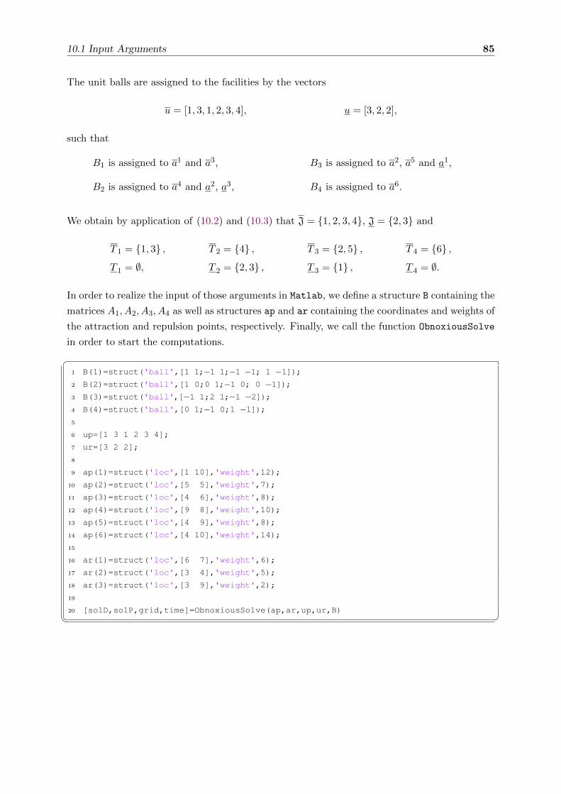
10.1 Input Arguments 85
The unit balls are assigned to the facilities by the vectors
u = [1, 3, 1, 2, 3, 4], u = [3, 2, 2],
such that
B1 is assigned to a1 and a3,
B2 is assigned to a4 and a2, a3,
B3 is assigned to a2, a5 and a1,
B4 is assigned to a6.
We obtain by application of (10.2) and (10.3) that J = {1, 2, 3, 4}, J = {2, 3} and
T 1 = {1, 3} , T 2 = {4} , T 3 = {2, 5} , T 4 = {6} ,
T 1 = ∅, T 2 = {2, 3} , T 3 = {1} , T 4 = ∅.
In order to realize the input of those arguments in Matlab, we define a structure B containing the
matrices A1, A2, A3, A4 as well as structures ap and ar containing the coordinates and weights of
the attraction and repulsion points, respectively. Finally, we call the function ObnoxiousSolve
in order to start the computations.�1 B(1)=struct('ball',[1 1;−1 1;−1 −1; 1 −1]);2 B(2)=struct('ball',[1 0;0 1;−1 0; 0 −1]);3 B(3)=struct('ball',[−1 1;2 1;−1 −2]);4 B(4)=struct('ball',[0 1;−1 0;1 −1]);5
6 up=[1 3 1 2 3 4];
7 ur=[3 2 2];
8
9 ap(1)=struct('loc',[1 10],'weight',12);
10 ap(2)=struct('loc',[5 5],'weight',7);
11 ap(3)=struct('loc',[4 6],'weight',8);
12 ap(4)=struct('loc',[9 8],'weight',10);
13 ap(5)=struct('loc',[4 9],'weight',8);
14 ap(6)=struct('loc',[4 10],'weight',14);
15
16 ar(1)=struct('loc',[6 7],'weight',6);
17 ar(2)=struct('loc',[3 4],'weight',5);
18 ar(3)=struct('loc',[3 9],'weight',2);
19
20 [solD,solP,grid,time]=ObnoxiousSolve(ap,ar,up,ur,B)� �
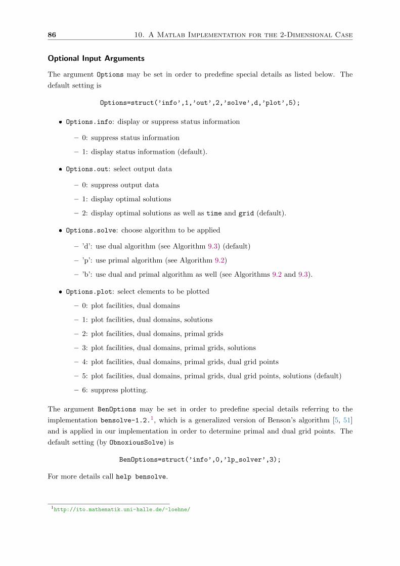
86 10. A Matlab Implementation for the 2-Dimensional Case
Optional Input Arguments
The argument Options may be set in order to predefine special details as listed below. The
default setting is
Options=struct(’info’,1,’out’,2,’solve’,d,’plot’,5);
� Options.info: display or suppress status information
– 0: suppress status information
– 1: display status information (default).
� Options.out: select output data
– 0: suppress output data
– 1: display optimal solutions
– 2: display optimal solutions as well as time and grid (default).
� Options.solve: choose algorithm to be applied
– ’d’: use dual algorithm (see Algorithm 9.3) (default)
– ’p’: use primal algorithm (see Algorithm 9.2)
– ’b’: use dual and primal algorithm as well (see Algorithms 9.2 and 9.3).
� Options.plot: select elements to be plotted
– 0: plot facilities, dual domains
– 1: plot facilities, dual domains, solutions
– 2: plot facilities, dual domains, primal grids
– 3: plot facilities, dual domains, primal grids, solutions
– 4: plot facilities, dual domains, primal grids, dual grid points
– 5: plot facilities, dual domains, primal grids, dual grid points, solutions (default)
– 6: suppress plotting.
The argument BenOptions may be set in order to predefine special details referring to the
implementation bensolve-1.2.1, which is a generalized version of Benson’s algorithm [5, 51]
and is applied in our implementation in order to determine primal and dual grid points. The
default setting (by ObnoxiousSolve) is
BenOptions=struct(’info’,0,’lp_solver’,3);
For more details call help bensolve.
1http://ito.mathematik.uni-halle.de/~loehne/

10.2 Output Arguments 87
� BenOptions.info: display information for bensolve
– 0: suppress display information for bensolve (default)
– 1: display information for bensolve
– 2: display more information for bensolve.
� BenOptions.lp_solver: select LP solver for bensolve
– 0: MATLAB linprog
– 1: cdd with criss-cross-method
– 2: cdd with simplex
– 3: glpk (revised simplex) (default).
10.2 Output Arguments
Depending on the chosen output option, the function ObnoxiousSolve returns the following
arguments (as far as they were determined):
1. When Options.out>0, then the calculated primal and dual solutions are displayed.
The structures solP and solD contain
� the optimal primal grid points x ∈ I ∩ X ,
� the optimal dual grid points y ∈ ID ∩ Y,
� the optimal objective value α,
obtained by executing the primal Algorithm 9.2 and the dual Algorithm 9.3, respectively.
2. If Options.out=2 then, additionally, the output arguments grid and time are displayed.
The fields of the structure grid contain
� the primal attraction grid points x ∈ I,
� the primal repulsion grid points x ∈ I,
� the dual attraction grid points y ∈ ID,
� the dual repulsion grid points y ∈ ID.
The fields of the structure time contain the running times for
� determining the primal and dual grid w.r.t. attraction,
� determining the primal and dual grid w.r.t. repulsion,
� solving the location problem (P) by executing the primal Algorithm 9.2,
� solving the location problem (P) by executing the dual Algorithm 9.3.

88 10. A Matlab Implementation for the 2-Dimensional Case
10.3 Subroutines of the Matlab Implementation
In this section we present some of the subroutines of the function ObnoxiousSolve.
1. For a matrix A associated with the unit ball B ={x ∈ R2
∣∣Ax ≤ 1}, the subroutine
DualBall determines a matrix D, whose rows contain the extreme points of B. The
matrix D represents equivalently the matrix associated with the dual unit ball B∗ ={x ∈ R2
∣∣Dx ≤ 1}.�1 function [D]=DualBall(A)
2 A=unique(A,'rows');
3 k = convhull(A(:,1),A(:,2));
4 Q=A(k,1:2);
5 D=zeros(size(Q,1)−1,2);6 for i=1:size(Q,1)−17 x=linsolve([Q(i,:);Q(i+1,:)],[1;1]);
8 D(i,:)=x';
9 end� �Amongst others, this subroutine is used for determining the matrices associated with
the dual unit balls B∗1 , . . . , B∗J , which then are stored in the field B(j).dualBall for all
j = 1, . . . , J .
2. The subroutine Domain determines the extreme points of dom g∗ and domh∗.
By defining vectors w ∈ R|J|+ and w ∈ R|J|+ such that
w(j) : =∑m∈T j
wm, ∀j ∈ J,
w(j) : =∑m∈T j
wm, ∀j ∈ J,
the domains of g∗ and h∗ can be determined by
dom g∗ =∑j∈J
B∗j · w(j), domh∗ =∑j∈J
B∗j · w(j).
Compared to (5.5) the number of unit balls, which are to be summed up, reduces from M
to∣∣J∣∣ and from M to
∣∣J∣∣, since each ball is taken into account only once. Especially in
the case that J = 1, see Remark 5.3, we have
dom g∗ = B∗ ·M∑m=1
wm, domh∗ = B∗ ·M∑m=1
wm.

10.3 Subroutines of the Matlab Implementation 89
�1 function [Bp,Br,B]=Domain(ap,ar,B,up,ur)
2 Bp=[0 0]; Br=[0 0];
3 Mp=length(up); Mr=length(ur);
4 for m=1:Mp
5 for i=1:size(B,2)
6 if up(m)==i
7 B(i).pweight=B(i).pweight+ap(m).weight;
8 end
9 end
10 end
11 for i=1:size(B,2)
12 Bp=minksum(Bp,B(i).pweight*B(i).ball);
13 end
14 for m=1:Mr
15 for i=1:size(B,2)
16 if ur(m)==i
17 B(i).rweight=B(i).rweight+ar(m).weight;
18 end
19 end
20 end
21 for i=1:size(B,2)
22 Br=minksum(Br,B(i).rweight*B(i).ball);
23 end� �3. Taking into account the matrices Bp and Br, whose rows contain the extreme points of
dom g∗ and domh∗, respectively, the subroutine Finite evaluates the condition for the
existence of a finite optimal solution of the location problem (P), based on Theorem 5.2.
Let Bcon be the matrix associated with dom g∗, i.e., dom g∗ ={y ∈ R2
∣∣Bcony ≤ 1}
. Then
it holds
domh∗ ⊆ dom g∗ ⇔ ∀y ∈ ext(domh∗) : Bcony ≤ 1.
The subroutine Finite returns a decision variable L which is defined as
L :=
1, if domh∗ ⊆ dom g∗,
0, if otherwise.
�1 function[L]=Finite(Bp,Br)
2 k = convhull(Bp(:,1),Bp(:,2));
3 Bp=[Bp(k,1),Bp(k,2)];
4 Bp con=dual ball(Bp);
5 if Bp con*Br'<=ones(size(Bp con,1),size(Br,1))
6 L=0;
7 else
8 L=1;
9 end� �

90 10. A Matlab Implementation for the 2-Dimensional Case
4. Based on equation (4.9), the subroutine Gauge determines the gauge distance, associated
with the unit ball B ={x ∈ R2
∣∣Ax ≤ 1}, A ∈ Rr×2, between a point x and the origin:
γB(x) = maxy∈B∗
〈x, y〉 = maxy∈ext(B∗)
〈x, y〉 = maxi=1,...,r
[Ax]i.
�1 function [gaugedist]=Gauge(A,x)
2 gaugedist=max(A*x);� �5. Based on Corollary 5.13, the function GetPrimal determines for each optimal dual grid
point y ∈ ID the corresponding primal solutions, given by the elementary convex set
∂g∗(y). We obtain
x ∈ ∂g∗(y) =
M⋂m=1
[am +NwmB
∗m
(ym)],
where for all m = 1, . . . ,M
(x− am) ∈ NwmB∗m
(ym)⇔ ∀y ∈ wmB∗m : 〈x− am, y − ym〉 ≤ 0
⇔ ∀y ∈ ext(wmB∗m) : 〈x, y − ym〉 ≤ 〈am, y − ym〉 .
Since the rows of the matrix Am, associated with the unit ball Bm, contain the extreme
points of the dual unit ball B∗m, we obtain
∂g∗(y) ={x ∈ R2
∣∣ ∀m = 1, . . . ,M ; ∀i = 1, . . . , rm :⟨x,wm[Am]i − ym
⟩≤⟨am, wm[Am]i − ym
⟩}.
�1 function [B,b]=GetPrimal(yp,ap,Mp)
2 B=[];b=[];
3 for m=1:Mp
4 Bm=ap(m).weight*ap(m).ball;
5 for i=1:size(Bm,1)
6 By=Bm(i,:)−yp(m,:);7 B=[B;By];
8 b=[b;By*(ap(m).loc)'];
9 end
10 end� �The determination of the corresponding extreme points can be realized by vertex enumer-
ation [4, 24, 51].
6. Based on Proposition 5.8 and Corollary 5.12, the function GetDual determines for each
optimal primal grid point x ∈ I the corresponding dual solutions, given by the elementary
convex set ∂h(x). Since the extreme points of the dual balls B∗1, . . . , B∗M coincide with the

10.3 Subroutines of the Matlab Implementation 91
rows of the matrices A1, . . . , AM associated with the respective primal balls B1, . . . , BM ,
we obtain
∂h(x) =
M∑m=1
argmaxym∈wmB
∗m
⟨x− am, ym
⟩where
ext(wmB∗m) =
{wm[Am]1, . . . , wm[Am]rm
}.
�1 function Y=GetDual(x,ar,Mr)
2 Y=[0 0];
3 for m=1:Mr
4 Ym=[];
5 u=ar(m).weight*ar(m).ball;
6 d=u*(x−ar(m).loc)';7 z=max(d);
8 ind=find(d>z−0.0001);9 for i=1:length(ind)
10 Ym=[Ym;u(ind(i),:)];
11 end
12 Y=minksum(Y,Ym);
13 end� �Overview on the Program Structure
The function ObnoxiousSolve is organized as follows:
0. The subroutine SetDefault sets the default options for the function ObnoxiousSolve.
1. For a matrix A, associated with the unit ball B ={x ∈ R2
∣∣Ax ≤ 1}, the subroutine
DualBall determines a matrix D, whose rows contain the extreme points of B. The matrix
D represents equivalently the matrix associated with the dual ballB∗ ={x ∈ R2
∣∣Dx ≤ 1}.
2. The function Domain determines the extreme points of dom g∗ and domh∗.
3. The function Finite evaluates the finiteness condition domh∗ ⊆ dom g∗ (see Theorem 5.2
and step 1 in the Algorithms 9.2 and 9.3). If the condition is not satisfied, the program
displays ”Solution is INFINITE.” before quitting. Otherwise, if the finiteness condition
is true, the program displays ”Solution is finite.” and starts the determination of
optimal solutions.
4. SolvePrimal executes the steps 2, 3 and 4 in the primal Algorithm 9.2 in order to deter-
mine the optimal primal and dual grid points for the dual pair of optimization problems
(P) and (D).

92 10. A Matlab Implementation for the 2-Dimensional Case
a) The subroutine Gauge is applied in order to calculate the objective values h(x) for all
x ∈ I (step 3 in Algorithm 9.2) and for determining the matrix Y , whose columns
generate the recession cone 0+ epi g, see Section 7.
b) The function bensolve determines the primal and the dual grid points x ∈ I and
y ∈ ID as well as the objective values g(x) and g∗(y), see step 2 in Algorithm 9.2.
The subroutine is called by bensolve(P,B,b,Y,[],c,ben_opt). The required input
arguments P,B,b,Y,c can be chosen as they are presented in Chapter 7.
c) Based on Proposition 5.8 and Corollary 5.12, the function GetDual determines for
each optimal primal grid point x ∈ I the corresponding dual solutions, given by the
elementary convex set ∂h(x), see step 4 in Algorithm 9.2.
5. SolveDual executes the steps 2, 3 and 4 in the dual Algorithm 9.3, in order to determine
the optimal primal and dual grid points for the dual pair of optimization problems (P)
and (D).
a) The subroutine Gauge is applied in order to determine the matrix Y , whose columns
generate the recession cone 0+ epih, see Section 7.
b) The function bensolve determines the primal and dual grid points x ∈ I and y ∈ IDas well as the objective values values h(x) and h∗(y), see step 2 in Algorithm 9.3.
c) Based on Corollary 5.13, the function GetPrimal determines for the optimal dual grid
points y ∈ ID the corresponding primal solutions given by the elementary convex set
∂g∗(y), see step 4 in Algorithm 9.3.
6. ObnoxiousPlot illustrates (depending on the predefined plot options) the existing facilities,
the primal grids w.r.t. attraction and repulsion, the dual domains w.r.t. attraction and
repulsion and the optimal primal and dual grid points.

10.3 Subroutines of the Matlab Implementation 93
Matlab Code of the Main Routine
�1 function [solD,solP,grid,time]=ObnoxiousSolve(ap,ar,up,ur,B,Options,BenOptions)
2
3 display('*******************************')
4 display('* ObnoxiousSolve *')
5 display('*******************************')
6
7 solP=[];
8 solD=[];
9 grid=[];
10 time=[];
11
12 Mp=length(up);
13 Mr=length(ur);
14
15 %%%%%%%%%%%%%%%%%%%%%%%%%%%%%%%%%%%%%
16 % 0. set (default) options
17 %%%%%%%%%%%%%%%%%%%%%%%%%%%%%%%%%%%%%
18 [Options,BenOptions]=SetDefault(Options,BenOptions);
19
20 %%%%%%%%%%%%%%%%%%%%%%%%%%%%%%%%%%%%%
21 % 1. determine dual balls and initialize
22 %%%%%%%%%%%%%%%%%%%%%%%%%%%%%%%%%%%%%
23 if Options.info>0
24 display('DETERMINING DUAL BALLS')
25 end
26 for i=1:size(B,2)
27 B(i).pweight=0;
28 B(i).rweight=0;
29 B(i).dualBall=DualBall(B(i).ball);
30 end
31 for m=1:Mp
32 ap(m).ball=B(up(m)).ball;
33 ap(m).dualBall=B(up(m)).dualBall;
34 end
35 for m=1:Mr
36 ar(m).ball=B(ur(m)).ball;
37 ar(m).dualBall=B(ur(m)).dualBall;
38 end
39 if Options.info>0
40 display('done.')
41 end
42
43 %%%%%%%%%%%%%%%%%%%%%%%%%%%%%%%%%%%%%
44 % 2. determine domain g* and domain h*45 %%%%%%%%%%%%%%%%%%%%%%%%%%%%%%%%%%%%%
46 if Options.info>0
47 display('DETERMINING DOMAINS OF g* AND h*...')
48 end

94 10. A Matlab Implementation for the 2-Dimensional Case
49 [Bp,Br,B]=Domain(ap,ar,B,up,ur);
50 if Options.info>0
51 display('done.')
52 end
53
54 %%%%%%%%%%%%%%%%%%%%%%%%%%%%%%%%%%%%%
55 % 3. check if dom h* subset of dom g*56 %%%%%%%%%%%%%%%%%%%%%%%%%%%%%%%%%%%%%
57 if Options.info>0
58 display('CHECKING FINITENESS...')
59 end
60 L=Finite(Bp,Br);
61 if L>0
62 display('Solution is INFINITE.')
63 else
64 if Options.info>0
65 display('Solution is finite.')
66 end
67
68 %%%%%%%%%%%%%%%%%%%%%%%%%%%%%%%%%%%%%
69 % 4./5. solve primal and/or dual problem
70 %%%%%%%%%%%%%%%%%%%%%%%%%%%%%%%%%%%%%
71 if options.solve=='p'
72 [solP,grid.primal att,grid.dual att,time.att grid,...
73 time.primal solve]=SolvePrimal(ap,ar,Options,BenOptions);
74 elseif options.solve=='d'
75 [solD,grid.primal rep,grid.dual rep,time.rep grid,...
76 time.dual solve]=SolveDual(ap,ar,Mp,Mr,Options,BenOptions);
77 elseif options.solve=='b'
78 [solP,grid.primal att,grid.dual att,time.att grid,...
79 time.primal solve]=SolvePrimal(ap,ar,Options,BenOptions);
80 [solD,grid.primal rep,grid.dual rep,time.rep grid,...
81 time.dual solve]=SolveDual(ap,ar,Mp,Mr,Options,BenOptions);
82 else
83 error('Invalid entry in Option.solve chosen.')
84 end
85 end
86
87 %%%%%%%%%%%%%%%%%%%%%%%%%%%%%%%%%%%%%
88 % 6. plot
89 %%%%%%%%%%%%%%%%%%%%%%%%%%%%%%%%%%%%%
90 ObnoxiousPlot(ap,ar,solP,solD,grid,Bp,Br,Options)� �

10.4 Examples 95
10.4 Examples
In this section we illustrate some examples solved by ObnoxiousSolve. The first Example 10.4
serves as a general explanation concerning the interpretation of the output arguments. The
Examples 10.5, 10.6, 10.7 and 10.8 demonstrate the difference between the primal Algorithm 9.2
and the dual Algorithm 9.3 concerning time complexity. The case that no finite solution exists
is illustrated in Example 10.9.
Example 10.4. For the data of Example 10.3 the implementation ObnoxiousSolve returns the
following output:�1 time =
2 att grid: 1.4920
3 primal solve: 0.0112
4 rep grid: 0.1548
5 dual solve: 0.1650
6
7 grid =
8 primal att: [3x33 double]
9 dual att: [3x45 double]
10 primal rep: [3x9 double]
11 dual rep: [3x16 double]
12
13 solP.primal =
14 4.0000 10.0000
15
16 solP.dual =
17 −16 43
18 −4 31
19
20 solP.obj val =
21 −14.000022
23 solD.primal =
24 4 10
25
26 solD.dual =
27 −16.0000 43.0000
28 −4 31
29
30 solD.obj val =
31 −14� �Both, the primal Algorithm 9.2 as well as the dual Algorithm 9.3, lead to the optimal primal
grid point x = (4, 10)T , the optimal dual grid points y = (−16, 43)T and y = (−4, 31)T and the
optimal objective value α = −14.
Moreover, the primal Algorithm 9.2 returns the sets I and ID of 33 primal and 45 dual grid
points w.r.t. attraction, where each x ∈ I and y ∈ ID has three entries: its coordinates in
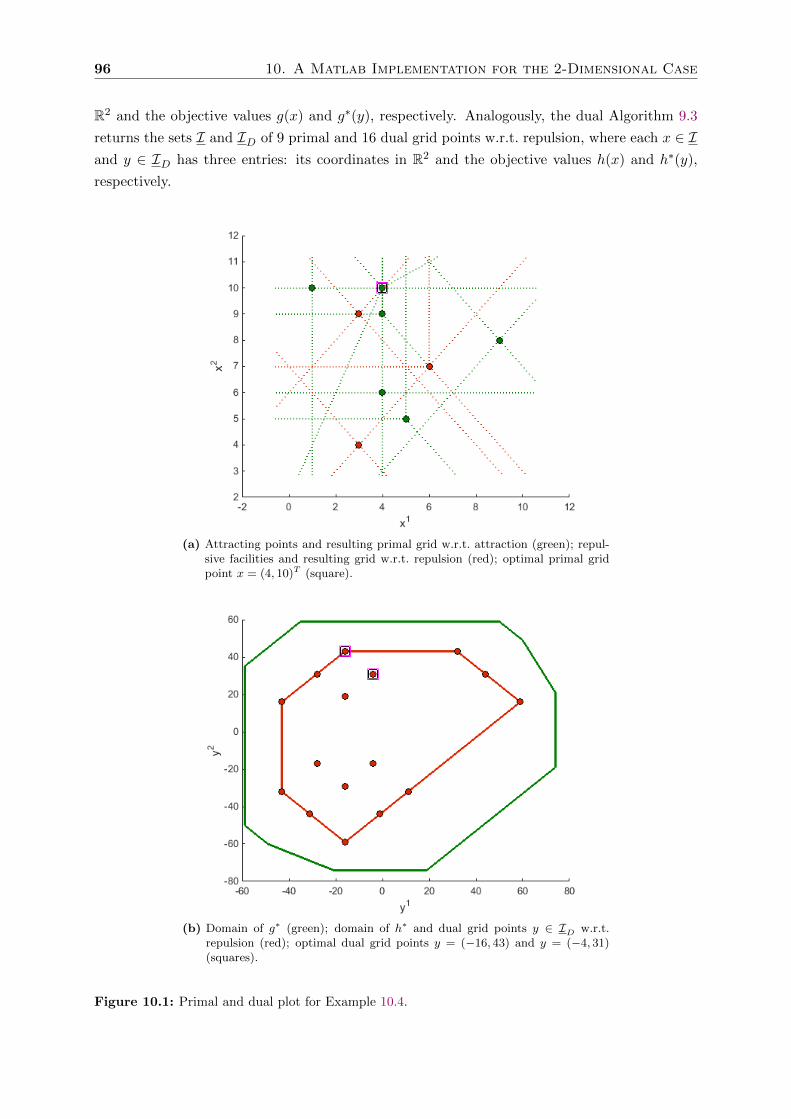
96 10. A Matlab Implementation for the 2-Dimensional Case
R2 and the objective values g(x) and g∗(y), respectively. Analogously, the dual Algorithm 9.3
returns the sets I and ID of 9 primal and 16 dual grid points w.r.t. repulsion, where each x ∈ Iand y ∈ ID has three entries: its coordinates in R2 and the objective values h(x) and h∗(y),
respectively.
(a) Attracting points and resulting primal grid w.r.t. attraction (green); repul-sive facilities and resulting grid w.r.t. repulsion (red); optimal primal gridpoint x = (4, 10)T (square).
(b) Domain of g∗ (green); domain of h∗ and dual grid points y ∈ ID w.r.t.repulsion (red); optimal dual grid points y = (−16, 43) and y = (−4, 31)(squares).
Figure 10.1: Primal and dual plot for Example 10.4.

10.4 Examples 97
Example 10.5. Consider the location problem (P) with ten attracting and two repulsive facil-
ities as follows:�1 B(1)=struct('ball',[1 1;−1 1;−1 −1; 1 −1]);2 B(2)=struct('ball',[1 0;0 1;−1 0; 0 −1]);3 B(3)=struct('ball',[−1 1;2 1;−1 −2]);4 B(4)=struct('ball',[0 1;−1 0;1 −1]);5
6 up=[4 2 4 3 1 1 4 2 2 4];
7 ur=[3 1];
8
9 ap(1) =struct('loc',[8 4],'weight',2);
10 ap(2) =struct('loc',[4 3],'weight',2);
11 ap(3) =struct('loc',[7 12],'weight',3);
12 ap(4) =struct('loc',[2 1],'weight',1);
13 ap(5) =struct('loc',[12 9],'weight',1);
14 ap(6) =struct('loc',[12 2],'weight',2);
15 ap(7) =struct('loc',[5 6],'weight',1);
16 ap(8) =struct('loc',[4 4],'weight',1);
17 ap(9) =struct('loc',[12 1],'weight',3);
18 ap(10)=struct('loc',[5 8],'weight',3);
19
20 ar(1) =struct('loc',[2 9],'weight',3);
21 ar(2) =struct('loc',[2 6],'weight',3);
22
23 [solD,solP,grid,time]=ObnoxiousSolve(ap,ar,up,ur,B,struct('solve','b'),[]);� �We obtain the following results:�1 time =
2 att grid: 5.3228
3 primal solve: 0.0051
4 rep grid: 0.0619
5 dual solve: 0.0257
6
7 grid =
8 primal att: [3x80 double]
9 dual att: [3x10² double]
10 primal rep: [3x3 double]
11 dual rep: [3x7 double]� �Obviously, the time complexity is mainly influenced by the number of grid points w.r.t. attrac-
tion. We have 80 primal and 102 dual grid points w.r.t. attraction (computed by executing the
primal Algorithm 9.2) and only 3 primal and 7 dual grid points w.r.t. repulsion (computed by
executing the dual Algorithm 9.3). Hence, for this example it seems to be advantageous to apply
the dual algorithm.
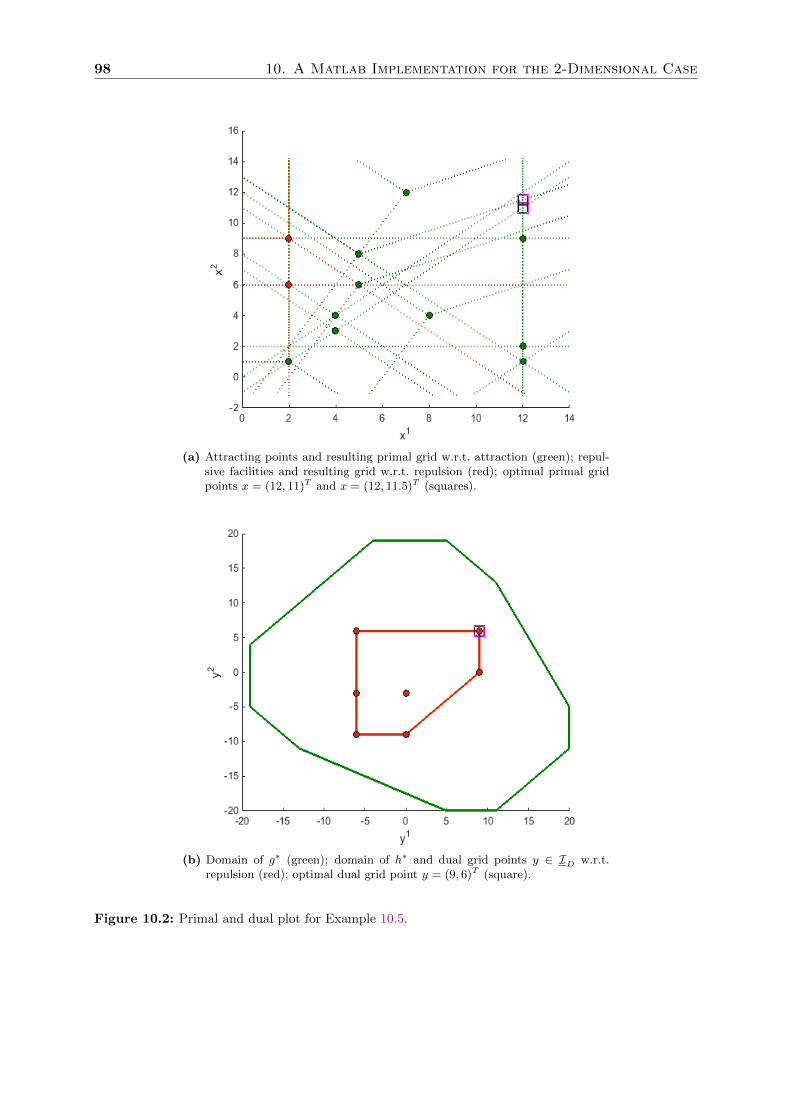
98 10. A Matlab Implementation for the 2-Dimensional Case
(a) Attracting points and resulting primal grid w.r.t. attraction (green); repul-sive facilities and resulting grid w.r.t. repulsion (red); optimal primal gridpoints x = (12, 11)T and x = (12, 11.5)T (squares).
(b) Domain of g∗ (green); domain of h∗ and dual grid points y ∈ ID w.r.t.repulsion (red); optimal dual grid point y = (9, 6)T (square).
Figure 10.2: Primal and dual plot for Example 10.5.

10.4 Examples 99
Example 10.6. Consider the location problem (P) with three attracting and ten repulsive
facilities as follows:�1 B(1)=struct('ball',[1 1;−1 1;−1 −1; 1 −1]);2 B(2)=struct('ball',[1 0;0 1;−1 0; 0 −1]);3 B(3)=struct('ball',[−1 1;2 1;−1 −2]);4 B(4)=struct('ball',[0 1;−1 0;1 −1]);5
6 up=[2 3 4];
7 ur=[2 1 4 4 4 2 3 3 1 2];
8
9 ap(1) =struct('loc',[4 11],'weight',10);
10 ap(2) =struct('loc',[5 6],'weight',8);
11 ap(3) =struct('loc',[8 3],'weight',4);
12
13 ar(1) =struct('loc',[11 8],'weight',1);
14 ar(2) =struct('loc',[4 6],'weight',2);
15 ar(3) =struct('loc',[11 9],'weight',1);
16 ar(4) =struct('loc',[9 6],'weight',1);
17 ar(5) =struct('loc',[2 10],'weight',1);
18 ar(6) =struct('loc',[3 5],'weight',1);
19 ar(7) =struct('loc',[7 7],'weight',1);
20 ar(8) =struct('loc',[5 7],'weight',1);
21 ar(9) =struct('loc',[12 9],'weight',1);
22 ar(10)=struct('loc',[10 2],'weight',1);
23
24 [solD,solP,grid,time]=ObnoxiousSolve(ap,ar,up,ur,B,struct('solve','b'),[]);� �We obtain the following results:�1 time =
2 att grid: 0.0489
3 primal solve: 0.0013
4 rep grid: 2.2252
5 dual solve: 0.0424
6
7 grid =
8 primal att: [3x8 double]
9 dual att: [3x14 double]
10 primal rep: [3x88 double]
11 dual rep: [3x113 double]� �Obviously, the time complexity is mainly influenced by the number of grid points w.r.t. repulsion.
We have 8 primal and 14 dual grid points w.r.t. attraction (computed by executing the primal
Algorithm 9.2) but 88 primal and 113 dual grid points w.r.t. repulsion (computed by executing
the dual Algorithm 9.3). Hence, for this example it seems to be advantageous to apply the
primal algorithm.

100 10. A Matlab Implementation for the 2-Dimensional Case
(a) Attracting points and resulting primal grid w.r.t. attraction (green); repul-sive facilities and resulting grid w.r.t. repulsion (red); optimal primal gridpoint x = (5, 10)T (square).
(b) Domain of g∗ (green); domain of h∗ and dual grid points y ∈ ID w.r.t.repulsion (red); optimal dual grid points y = (−3, 6)T , y = (−2, 7)T , y =(0, 6)T , y = (1, 7)T (squares).
Figure 10.3: Primal and dual plot for Example 10.6.

10.4 Examples 101
Example 10.7. Consider the location problem (P) with ten attracting and ten repulsive facil-
ities as follows:�1 B(1)=struct('ball',[1 1;−1 1;−1 −1; 1 −1]);2 B(2)=struct('ball',[1 0;0 1;−1 0; 0 −1]);3 B(3)=struct('ball',[−1 1;2 1;−1 −2]);4 B(4)=struct('ball',[0 1;−1 0;1 −1]);5
6 up=[1 3 2 1 1 4 3 2 4 1];
7 ur=[3 4 2 2 2 4 4 1 1 2];
8
9 ap(1) =struct('loc',[15 15],'weight',7);
10 ap(2) =struct('loc',[4 12],'weight',4);
11 ap(3) =struct('loc',[3 5],'weight',10);
12 ap(4) =struct('loc',[2 5],'weight',1);
13 ap(5) =struct('loc',[9 1],'weight',10);
14 ap(6) =struct('loc',[4 2],'weight',4);
15 ap(7) =struct('loc',[10 3],'weight',11);
16 ap(8) =struct('loc',[7 6],'weight',1);
17 ap(9) =struct('loc',[6 1],'weight',6);
18 ap(10)=struct('loc',[16 13],'weight',1);
19
20 ar(1) =struct('loc',[2 16],'weight',5);
21 ar(2) =struct('loc',[11 3],'weight',5);
22 ar(3) =struct('loc',[7 6],'weight',5);
23 ar(4) =struct('loc',[1 1],'weight',4);
24 ar(5) =struct('loc',[13 11],'weight',5);
25 ar(6) =struct('loc',[15 16],'weight',2);
26 ar(7) =struct('loc',[14 12],'weight',3);
27 ar(8) =struct('loc',[2 16],'weight',2);
28 ar(9) =struct('loc',[13 15],'weight',1);
29 ar(10)=struct('loc',[3 11],'weight',3);
30
31 [solD,solP,grid,time]=ObnoxiousSolve(ap,ar,up,ur,B,struct('solve','b'),[]);� �We obtain the following results:�1 time =
2 att grid: 6.5522
3 primal solve: 0.0165
4 rep grid: 4.1830
5 dual solve: 0.0607
6
7 grid =
8 primal att: [3x10⁶ double]
9 dual att: [3x129 double]
10 primal rep: [3x94 double]
11 dual rep: [3x121 double]� �Obviously, the time complexity is mainly influenced by both, the number of grid points w.r.t.

102 10. A Matlab Implementation for the 2-Dimensional Case
attraction and the number of grid points w.r.t. repulsion. We have 106 primal and 129 dual grid
points w.r.t. attraction (computed by executing the primal Algorithm 9.2) and 94 primal and
121 dual grid points w.r.t. repulsion (computed by executing the dual Algorithm 9.3). Hence,
both algorithms seem to be comparable concerning running times for this example.
(a) Attracting points and resulting primal grid w.r.t. attraction (green); repul-sive facilities and resulting grid w.r.t. repulsion (red); optimal primal gridpoints x = (9, 3)T and x = (9, 2.5)T (squares).
(b) Domain of g∗ (green); domain of h∗ and dual grid points y ∈ ID w.r.t.repulsion (red); optimal dual grid point y = (−6,−28)T (square).
Figure 10.4: Primal and dual plot for Example 10.7.
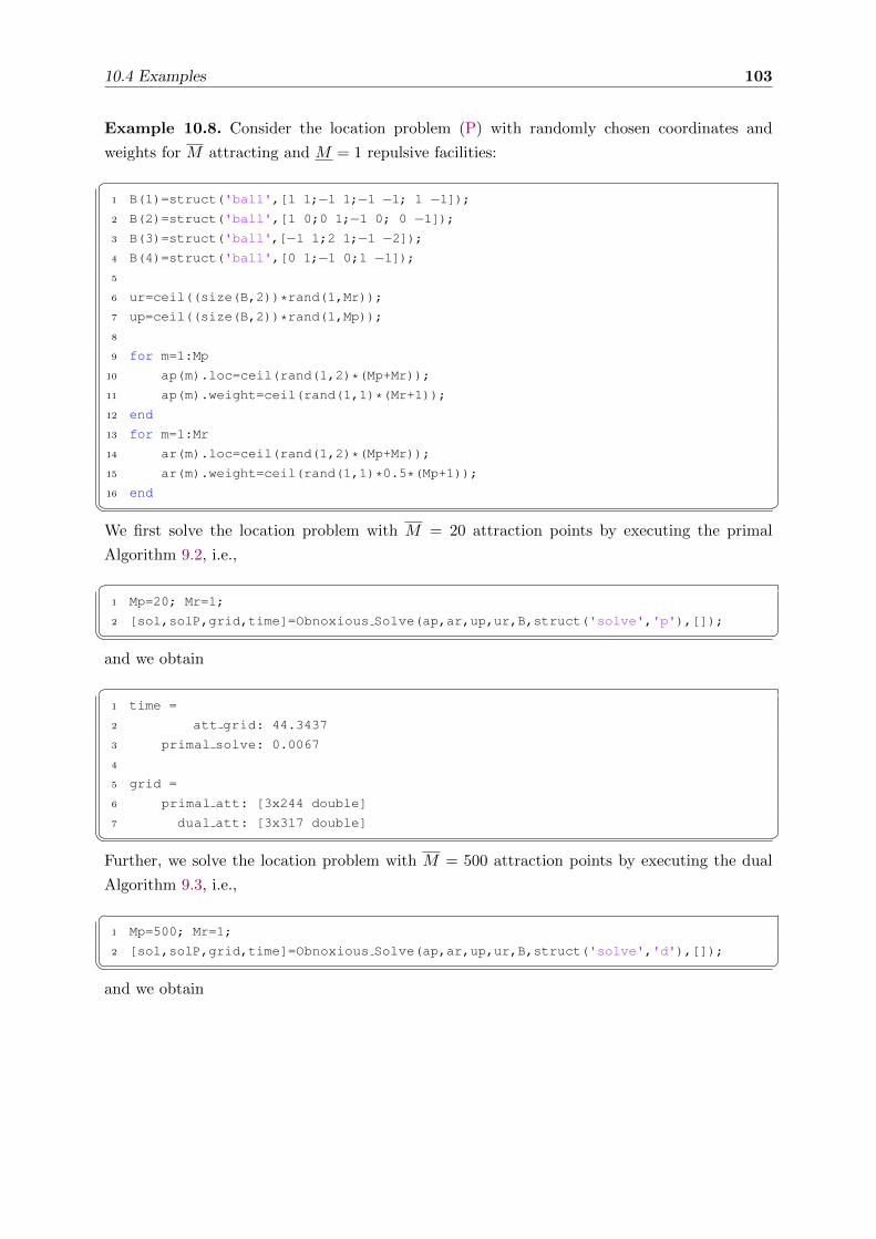
10.4 Examples 103
Example 10.8. Consider the location problem (P) with randomly chosen coordinates and
weights for M attracting and M = 1 repulsive facilities:�1 B(1)=struct('ball',[1 1;−1 1;−1 −1; 1 −1]);2 B(2)=struct('ball',[1 0;0 1;−1 0; 0 −1]);3 B(3)=struct('ball',[−1 1;2 1;−1 −2]);4 B(4)=struct('ball',[0 1;−1 0;1 −1]);5
6 ur=ceil((size(B,2))*rand(1,Mr));
7 up=ceil((size(B,2))*rand(1,Mp));
8
9 for m=1:Mp
10 ap(m).loc=ceil(rand(1,2)*(Mp+Mr));
11 ap(m).weight=ceil(rand(1,1)*(Mr+1));
12 end
13 for m=1:Mr
14 ar(m).loc=ceil(rand(1,2)*(Mp+Mr));
15 ar(m).weight=ceil(rand(1,1)*0.5*(Mp+1));
16 end� �We first solve the location problem with M = 20 attraction points by executing the primal
Algorithm 9.2, i.e.,�1 Mp=20; Mr=1;
2 [sol,solP,grid,time]=Obnoxious Solve(ap,ar,up,ur,B,struct('solve','p'),[]);� �and we obtain�1 time =
2 att grid: 44.3437
3 primal solve: 0.0067
4
5 grid =
6 primal att: [3x244 double]
7 dual att: [3x317 double]� �Further, we solve the location problem with M = 500 attraction points by executing the dual
Algorithm 9.3, i.e.,�1 Mp=500; Mr=1;
2 [sol,solP,grid,time]=Obnoxious Solve(ap,ar,up,ur,B,struct('solve','d'),[]);� �and we obtain

104 10. A Matlab Implementation for the 2-Dimensional Case
�1 time =
2 rep grid: 0.0153
3 dual solve: 17.3229
4
5 grid =
6 primal rep: [3x1 double]
7 dual rep: [3x3 double]� �When solving the location problem (P) with 20 attraction points by executing the primal Algo-
rithm 9.2, the time complexity consists mainly of determining the 244 primal and 317 dual grid
points w.r.t. attraction. When solving the location problem (P) with a much greater amount of
500 attraction points by executing the dual Algorithm 9.3, the time complexity consists mainly
of determining the optimal solutions. There are only one primal and three dual grid points.
For each grid point, a linear optimization problem is to be solved in step 3 of Algorithm 9.3,
where the running time for each sub-problem depends on the number of attraction points, see
also Section 9.3.
As we can see, solving the problem with M = 20 attraction points by executing the primal
algorithm needs more than twice the time for solving the problem with M = 500 attraction
points by executing the dual algorithm. Hence, when there is a large number of attracting
facilities and a small number of repulsive ones, then it is beneficial to apply the dual Algorithm
instead of the primal one.
Example 10.9. Consider the location problem (P) with five attracting and five repulsive facil-
ities as follows:�1 B(1)=struct('ball',[1 1;−1 1;−1 −1; 1 −1]);2 B(2)=struct('ball',[1 0;0 1;−1 0; 0 −1]);3 B(3)=struct('ball',[−1 1;2 1;−1 −2]);4 B(4)=struct('ball',[0 1;−1 0;1 −1]);5
6 up=[2 3 2 3 3];
7 ur=[1 2 4 4 1];
8
9 ap(1)=struct('loc',[3 5],'weight',1);
10 ap(2)=struct('loc',[10 2],'weight',1);
11 ap(3)=struct('loc',[4 2],'weight',3);
12 ap(4)=struct('loc',[4 10],'weight',6);
13 ap(5)=struct('loc',[1 8],'weight',2);
14
15 ar(1)=struct('loc',[5 6],'weight',3);
16 ar(2)=struct('loc',[5 10],'weight',1);
17 ar(3)=struct('loc',[8 7],'weight',2);
18 ar(4)=struct('loc',[7 7],'weight',1);
19 ar(5)=struct('loc',[2 10],'weight',1);
20
21 [sol,solP,grid,time]=ObnoxiousSolve(ap,ar,up,ur,B,struct('solve','b'),[]);� �
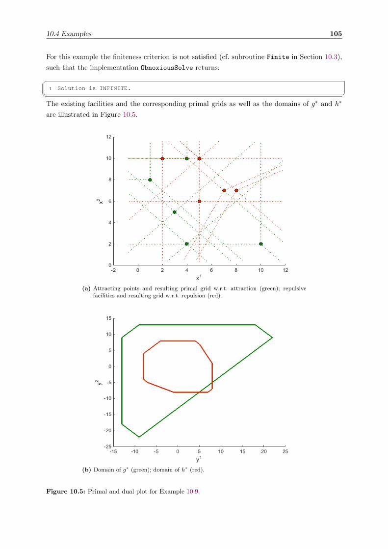
10.4 Examples 105
For this example the finiteness criterion is not satisfied (cf. subroutine Finite in Section 10.3),
such that the implementation ObnoxiousSolve returns:�1 Solution is INFINITE.� �
The existing facilities and the corresponding primal grids as well as the domains of g∗ and h∗
are illustrated in Figure 10.5.
(a) Attracting points and resulting primal grid w.r.t. attraction (green); repulsivefacilities and resulting grid w.r.t. repulsion (red).
(b) Domain of g∗ (green); domain of h∗ (red).
Figure 10.5: Primal and dual plot for Example 10.9.


Chapter 11Conclusion
In this thesis we present a new approach for solving the non-convex location problem (P) with
obnoxious facilities. This approach is based on the special structure of (P) and the fact that the
objective function can be written as a d.c. function. By applying the duality theory by Toland
[121] and Singer [112] we obtain a suitable dual problem (D).
We introduce the concepts of primal and dual elementary convex sets with respect to attraction
and to repulsion, as well as corresponding grids and grid points.
Although, we consider a scalar optimization problem, we show the remarkable fact, that methods
from the field of linear vector optimization can be applied in order to determine those grid points
with respect to attraction and to repulsion.
The relationship between primal and dual elementary convex sets is described, based on results
from the field of geometric duality [56], by an inclusion reversing one-to-one mapping.
Moreover, we present properties of primal and dual elementary convex sets and state duality
assertions and discretization results based on the duality theory by Toland and Singer.
The obtained results are applied in order to formulate a dual and a primal algorithm, which
determine exact solutions by leading back the non-convex optimization problems to a finite
number of convex problems.
The developed algorithms are implemented as Matlab functions. It turns out that, in case
of few attraction points with a small amount of fundamental directions, the primal algorithm
is beneficial. Whereas, in case of few repulsive facilities with a small amount of fundamental
directions the dual algorithm is advantageous.
In this thesis we also consider the more general case of a constrained location problem (PH)
by introducing an indicator function. Analogously to the unconstrained case, we define a dual
problem (DH) as well as primal and dual elementary convex sets with respect to attraction and
to repulsion, taking into account the constraints. We show that most of the results obtained for
the unconstrained location problem can be generalized for the constrained case.
For future research, further improvements of the presented algorithms might be possible. Fur-
thermore, the case of round gauges may be studied in more detail. Many results obtained in

108 11. Conclusion
this research can in fact also be formulated for this case, but are not applicable for an algorithm
from the present point of view. Moreover, it seems to be suitable to consider further constraints,
such as barriers, which may influence travel time and travel costs, or forbidden regions for the
obnoxious facility. Also the problem of locating multiple obnoxious facilities may be discussed.
Another interesting future research may focus on the question, how the duality theory by Toland
and Singer may also be applied for different kinds of location problems with obnoxious facilities,
such as network problems or problems with center objective function.

Index
bensolve-1.2., 54, 86
Benson algorithm, 47, 54, 65, 67, 86
cone
generated, 15, 25
normal cone, 15, 21, 25, 37
recession, 15, 16, 49
d.c. problem, 27–29, 56
discretization, 41, 62
distance
Euclidean, 18
Manhattan, 18, 66–70
Tchebychev, 18
edge, 14
effective domain, 16, 25, 33, 38, 39, 58, 60,
74, 75, 79, 88
elementary convex set, 26, 37, 41, 44–46, 61–
64, 67, 74, 75, 77, 78, 90–92
epigraph, 16, 25, 43–45, 48, 49, 51, 53, 65,
67
extreme point, 14, 19, 26, 27, 38, 48, 54, 61,
66, 67
face
K-minimal, 43
exposed, 14, 25, 43–45, 54, 66, 67
proper, 14
facet, 14
Fenchel-Young inequality, 22
Fermat-Weber problem, 25, 41, 79
finiteness criterion, 33, 59, 60, 71–75, 80, 81,
91, 105
function
affine, 17, 33, 35
biconjugate, 22
closed, 16, 22
conjugate, 22–25, 32, 56
convex, 16
d.c., 12, 27
indicator function, 16, 17, 21, 24, 33, 35,
56
polyhedral, 16, 17, 20, 22, 33, 35, 41, 44,
57, 61
positively homogeneous, 16–18
proper, 16
subadditive, 16, 17
sublinear, 16, 17
support, 17, 19, 21, 24, 56–60
fundamental directions, 26, 50, 66
gauge
dual, 17–19
polyhedral, 12, 18, 19
round, 18
geometric duality, 43–45, 61
grid, 26, 38, 39, 45, 46, 61, 64, 77, 78
grid points, 26, 38, 41, 46, 54, 61, 62, 65–67,
69–76, 78–81, 91, 92
half-space, 14, 55, 60, 64

110 Index
infimal convolution, 24, 25, 31
lower image, 48, 51, 53, 54, 65–67
Minkowski functional, 11, 16, 17
optimality condition, 29, 40, 60
polytope, 14, 18
set
affine, 13, 14
boundary, 14
closed, 14
convex, 13
interior, 13
polar, 18, 19
polyhedral, 14–19, 26, 41, 44, 47, 48, 55,
62
relative interior, 13
subdifferentiabilityl, 20
subdifferential, 19–21, 23, 35, 57
subgradient, 19
sum rule for subdifferentials, 20
Toland-Singer dual problem, 32, 56
Toland-Singer duality, 28
triangle inequality, 17, 18
upper image, 47–49, 54, 65–67
vector optimization problem, 47–49, 51–54,
65–67
Bibliography
[1] F. Al-Khayyal, H. Tuy, and F. Zhou. Large-scale single facility continuous location by d.c.
optimization. Optimization, 51(2):271–292, 2002.
[2] A. D. Aleksandrov. On the surfaces representable as difference of convex functions. Siberian
Electronic Mathematical Reports, 9:360–376, 2012.
[3] S. Alzorba, C. Gunther, and N. Popovici. A special class of extended multicriteria location
problems, Optimization, 2013.
[4] C. B. Barber, D. P. Dobkin, and H. Huhdanpaa. The quickhull algorithm for convex hulls.
ACM Transactions on Mathematical Software, 22(4):469–483, 1996.
[5] H. P. Benson. An outer approximation algorithm for generating all efficient extreme points
in the outcome set of a multiple objective linear programming problem. Journal of Global
Optimization, 13(1):1–24, 1998.
[6] O. Berman and Z. Drezner. A note on the location of an obnoxious facility on a network.
European Journal of Operational Research, 120(1):215–217, 2000.
[7] O. Berman, Z. Drezner, and G. O. Wesolowsky. Minimum covering criterion for obnoxious
facility location on a network. Networks, 28(1):1–5, 1996.
[8] O. Berman and Q. Wang. Locating a semi-obnoxious facility with expropriation: minisum
criterion. Journal of the Operational Research Society, 58(3):378–390, 2006.
[9] O. Berman and Q. Wang. Locating a semi-obnoxious facility with expropriation. Comput-
ers & Operations Research, 35(2):392–403, 2008. Part Special Issue: Location Modeling
Dedicated to the memory of Charles S. ReVelle.
[10] M. Bischoff. Location of Connection Facilities. Shaker Verlag, 2008.
[11] R. Blanquero and E. Carrizosa. A D.C. biobjective location model. Journal of Global
Optimization, 23(2):139–154, 2002.
[12] J. Borwein and A. Lewis. Convex Analysis and Nonlinear Optimization. Springer, second
edition, 2006.

112 Bibliography
[13] J. Brimberg and H. Juel. A bicriteria model for locating a semi-desirable facility in the
plane. European Journal of Operational Research, 106(1):144–151, 1998.
[14] J. Brimberg and H. Juel. On locating a semi-desirable facility on the continuous plane.
International Transactions in Operational Research, 5:5966, 1998.
[15] D. J. Buchanan and G. O. Wesolowsky. Locating a noxious facility with respect to several
polygonal regions using asymmetric distances. IIE Transactions, 25:77–88, 1993.
[16] P. Cappanera. A survey on obnoxious facility location problems. Technical report, Uni-
versity of Pisa, 1999.
[17] E. Carrizosa and E. Conde. A fractional model for locating semi-desirable facilities on
networks. European Journal of Operational Research, 136(1):67–80, 2002.
[18] E. Carrizosa, E. Conde, and D. Romero-Morales. Location of a semiobnoxious facility.
A biobjective approach. In Rafael Caballero, Francisco Ruiz, and Ralph Steuer, editors,
Advances in Multiple Objective and Goal Programming, volume 455 of Lecture Notes in
Economics and Mathematical Systems, pages 338–346. Springer Berlin Heidelberg, 1997.
[19] E. Carrizosa and F. Plastria. Locating an undesirable facility by generalized cutting planes.
Mathematics of Operations Research, 23(3):680–694, 1998.
[20] E. Carrizosa and F. Plastria. Location of semi-obnoxious facilities. Studies in Locational
Analysis, 12:1–27, 1999.
[21] E. Carrizosa and F. Plastria. Dominators for multiple-objective quasiconvex maximization
problems. Journal of Global Optimization, 18(1):35–58, 2000.
[22] R. Chandrasekaran and A. Daughety. Location on tree networks: p-centre and n-dispersion
problems. Mathematics of Operations Research, 6(1):50–57, 1981.
[23] S. S. Chaudhry, S. T. McCormick, and I. D. Moon. Locating independent facilities with
maximum weight: Greedy heuristics. Omega, 14(5):383–389, 1986.
[24] P. C. Chen, P. Hansen, and B. Jaumard. On-line and off-line vertex enumeration by
adjacency lists. Operations Research Letters, 10(7):403–409, 1991.
[25] P. C. Chen, P. Hansen, B. Jaumard, and H. Tuy. Webers problem with attraction and
repulsion. Journal of Regional Science, 32:467–486, 1992.
[26] P. C. Chen, P. Hansen, B. Jaumard, and H. Tuy. Solution of the multisource weber and
conditional weber problems by d.-c. programming. Operations Research, 46(4):548–562,
1998.
[27] R. L. Church and R. S. Garfinkel. Locating an obnoxious facility on a network. Trans-
portation Science, 12(2):107–118, 1978.

Bibliography 113
[28] B. Dasarathy and L. J. White. A maxmin location problem. Operations Research,
28(6):1385–1401, 1980.
[29] Z. Drezner, editor. Facility location: A Survey of Applications and Methods. Springer
Series in Operations Research. Springer-Verlag, New York, 1995. A survey of applications
and methods.
[30] Z. Drezner and H. W. Hamacher, editors. Facility Location: Application and Theory.
Contributions to Management Science. Physica Verlag Heidelberg, 2002.
[31] Z. Drezner, K. Klamroth, A. Schobel, and G. O. Wesolowsky. The weber problem.
In Z. Drezner and H. Hamacher, editors, Facility Location - Applications and Theory.
Springer-Verlag, 2002.
[32] Z. Drezner and G. O. Wesolowsky. A maximin location problem with maximum distance
constraints. A I I E Transactions, 12(3):249–252, 1980.
[33] Z. Drezner and G. O. Wesolowsky. The location of an obnoxious facility with rectangular
distances. Journal of Regional Science, 23:241–248, 1983.
[34] Z. Drezner and G. O. Wesolowsky. Location of multiple obnoxious facilities. Transportation
Science, 19:193–202, 1985.
[35] Z. Drezner and G. O. Wesolowsky. The Weber problem on the plane with some negative
weights. INFOR, 29(2):87–99, 1991.
[36] R. Durier and Chr. Michelot. Geometrical properties of the Fermat-Weber problem.
European Journal of Operational Research, 20(3):332–343, 1985.
[37] H. A. Eiselt and G. Laporte. Objectives in location problems. In Z. Drezner, editor,
Facility Location, a Survey of Applications and Methods, Springer Series in Operations
Research. Springer, 1995.
[38] H. A. Eiselt and V. Marianov. Foundations of Location Analysis. Springer-Verlag, 2011.
[39] H. A. Eiselt and C.L. Sandbloom. Decision Analysis, Location Models, and Scheduling
Problems. Springer-Verlag, 2004.
[40] E. Erkut. The discrete p-dispersion problem. European Journal of Operational Research,
46:48–60, 1990.
[41] E. Erkut, T. Baptie, and B. v. Hohenbalken. The discrete p-maxian location problem.
Computers & Operations Research, 17(1):51–61, 1990.
[42] E. Erkut and S. Neuman. Analytical models for locating undesirable facilities. European
Journal of Operational Research, 40(3):275–291, 1989.
[43] A. J. Goldman and P. M. Dearing. Concepts of optimal location for partially noxious
facilities. Bulletin of the Operations Research Society of America, 23(1):B–31, 1975.

114 Bibliography
[44] S. L. Hakimi. Optimum distribution of switching centers in a communication network and
some related graph theoretic problems. Operations Research, 13(3):462–475, 1965.
[45] H. W. Hamacher. Mathematische Losungsverfahren fur planare Standortprobleme. Vieweg,
1995.
[46] H. W. Hamacher, S. Klamroth, K. Nickel, and A. Schobel. Library of location algorithms.
[47] H. W. Hamacher, M. Labb, S. Nickel, and A. J. V. Skriver. Multicriteria semi-obnoxious
network location problems (msnlp) with sum and center objectives. Annals of Operations
Research, 110(1-4):33–53, 2002.
[48] H. W. Hamacher and S. Nickel. Restricted planar location problems and applications.
Naval Research Logistics, 42:967–992, 1995.
[49] H. W. Hamacher and S. Nickel. Classification of location models. Location Science,
6(14):229–242, 1998.
[50] H. W. Hamacher, S. Nickel, and A. Schneider. Classification of location problems. Tech-
nical report, Location Science, 1996.
[51] A. Hamel, A. Lohne, and B. Rudloff. Benson type algorithms for linear vector optimization
and applications. Journal of Global Optimization, 59(4):811–836, 2013.
[52] P. Hansen, D. Peeters, D. Richard, and J.-F. Thisse. The minisum and minimax location
problems revisited. Operations Research, 33:1251–1265, 1985.
[53] P. Hansen, D. Peeters, and J. F. Thisse. On the location of an obnoxious facility. Sistemi
Urbani, 3:299–317, 1981.
[54] P. Hansen and J. F. Thisse. The generalized weber-rawls problem. In J. L. Brans, editor,
Operational Research 81 (Hamburg, 1981), pages 569–577. North-Holland, Amsterdam,
1981.
[55] P. Hartman. On functions representable as a difference of convex functions. Pacific Journal
of Mathematics, 9(3):707–713, 1959.
[56] F. Heyde. Geometric duality for convex vector optimization problems. Journal of Convex
Analysis, 20(3):813–832, 2013.
[57] J.-B. Hiriart-Urruty. From convex optimization to nonconvex optimization. Necessary
and sufficient conditions for global optimality. In F. H. Clarke, V. F. Demyanov, and
F. Giannessi, editors, Nonsmooth Optimization and Related Topics, volume 43 of Ettore
Majorana International Science Series, pages 219–239. Springer US, 1989.
[58] J.-B. Hiriart-Urruty. The deconvolution operation in convex analysis: an introduction.
Kibernetika i Sistemnyi Analiz, 30(4):97–104, 190, 1994.

Bibliography 115
[59] J.-B. Hiriart-Urruty and C. Lemarechal. Convex analysis and minimization algorithms I.
Fundamentals, volume 305 of Grundlehren der Mathematischen Wissenschaften [Funda-
mental Principles of Mathematical Sciences]. Springer-Verlag, Berlin, 1993.
[60] J.-B. Hiriart-Urruty and C. Lemarechal. Convex analysis and minimization algorithms
II. Advanced theory and bundle methods, volume 306 of Grundlehren der Mathematis-
chen Wissenschaften [Fundamental Principles of Mathematical Sciences]. Springer-Verlag,
Berlin, 1993.
[61] R. Horst and N. V. Thoai. DC programming: overview. Journal of Optimization Theory
and Applications, 103(1):1–43, 1999.
[62] H. Idrissi, P. Loridan, and C. Michelot. Approximation of solutions for location problems.
Journal of Optimization Theory and Applications, 56(1):127–143, 1988.
[63] A. Jourani, C. Michelot, and M. Ndiaye. Efficiency for continuous facility location problems
with attraction and repulsion. Annals of Operations Research, 167(1):43–60, 2009.
[64] M. J. Kaiser and T. L. Morin. Center points, equilibrium positions, and the obnoxious
location problem. Journal of Regional Science, 33:237–249, 1993.
[65] J. Kalcsics. The multi-facility median problem with Pos/Neg weights on general graphs.
Computers & Operations Research, 38(3):674–682, 2011.
[66] E. Karasakal and D. Nadirler. An interactive solution approach for a bi-objective semi-
desirable location problem. Journal of Global Optimization, 42(2):177–199, 2008.
[67] J. Karkazis and P. Karagiorgis. The general problem of locating obnoxious facilities in the
plane. In Proceedings of the 11th IFORS Conference, Buenos Aires, Brazil, 1987.
[68] J. Karkazis and C. Papadimitriou. A branch-and-bound algorithm for the location of facil-
ities causing atmospheric pollution. European Journal of Operational Research, 58(3):363–
373, 1992.
[69] M. J. Katz, K. Kedem, and M. Segal. Improved algorithms for placing undesirable facilities.
Computers & Operations Research, 29(13):1859–1872, 2002.
[70] K. Klamroth. Single-facility location problems with barriers. Springer Series in Operations
Research. Springer-Verlag, New York, 2002.
[71] J. Krarup, D. Pisinger, and F. Plastria. Discrete location problems with push–pull objec-
tives. Discrete Applied Mathematics, 123(13):363–378, 2002.
[72] J. Krebs and S. Nickel. Extensions to the continuous ordered median problem. Mathe-
matical Methods of Operations Research, 71(2):283–306, 2010.
[73] M. J. Kuby. Programming models for facility dispersion: The p-dispersion and maxisum
dispersion problems. Geographical Analysis, 19:315–329, 1987.

116 Bibliography
[74] M. Labbe. Location of an obnoxious facility on a network: A voting approach. Networks,
20(2):197–207, 1990.
[75] A. Lohne. Bensolve – MOLP solver, v. 1.2. http://ito.mathematik.uni-halle.de/˜loehne.
[76] A. Lohne. Vector optimization with infimum and supremum. Vector Optimization.
Springer, Berlin, 2011.
[77] A. Lohne. Projection of polyhedral cones and linear vector optimization. Submitted, 2014.
[78] R. F. Love, J. G. Morris, and G. O. Wesolowsky, editors. Facility locations: Models and
Methods. Amsterdam: North-Holland, 1988.
[79] C. D. Maranas and C. Floudas. A global optimization method for webers problem with
attraction and repulsion. In W. W. Hager, D. W. Hearn, and P. M. Pardalos, editors,
Large Scale Optimization, pages 259–285. Springer US, 1994.
[80] J. E. Martınez-Legaz. Generalized conjugation and related topics. In Generalized convexity
and fractional programming with economic applications (Pisa, 1988), volume 345 of Lecture
Notes in Economics and Mathematical Systems, pages 168–197. Springer, Berlin, 1990.
[81] J. E. Martınez-Legaz and A. Seeger. A formula on the approximate subdifferential of the
difference of convex functions. Bulletin of the Australian Mathematical Society, 45(1):37–
41, 1992.
[82] J. E. Martınez-Legaz and I. Singer. An extension of d. c. duality theory, with an appendix
on ∗-subdifferentials. Optimization, 42(1):9–37, 1997.
[83] J. E. Martınez-Legaz and M. Volle. Duality in D.C. programming: the case of several D.C.
constraints. Journal of Mathematical Analysis and Applications, 237(2):657–671, 1999.
[84] A. Mehrez, Z. Sinuany-Stern, and A. Stulman. A single facility location problem with
a weighted maximin-minimax rectilinear distance. Computers & Operations Research,
12(1):51–60, 1985.
[85] A. Mehrez, Z. Sinuany-Stern, and A. Stulman. An enhancement of the Drezner-
Wesolowsky algorithm for single-facility location with maximin of rectilinear distance.
Journal of the Operational Research Society, 37:971–977, 1986.
[86] E. Melachrinoudis. Determining an optimum location for an undesirable facility in a
workroom environment. Applied Mathematical Modelling, 9:365–369, 1985.
[87] E. Melachrinoudis. An efficient computational procedure for the rectilinear maximin lo-
cation problem. Transportation Science, 22(3):217–223, 1988.
[88] E. Melachrinoudis. Bicriteria location of a semi-obnoxious facility. Computers & Industrial
Engineering, 37(3):581–593, 1999.

Bibliography 117
[89] E. Melachrinoudis and T. P. Cullinane. Locating an undesirable facility within a geo-
graphical region using the maximin criterion. Journal of Regional Science, 25:115–127,
1985.
[90] E. Melachrinoudis and T. P. Cullinane. Locating an obnoxious facility within a polygonal
region. Annals of Operations Research, 6:137–145, 1986.
[91] E. Melachrinoudis and T. P. Cullinane. Locating an undesirable facility with a minimax
criterion. European Journal of Operational Research, 24:239–246, 1986.
[92] E. Melachrinoudis and Z. Xanthopulos. Semi-obnoxious single facility location in Euclidean
space. Computers & Operations Research, 30(14):2191–2209, 2003.
[93] E. Minieka. Anticenters and antimedians of a network. Networks, 13:359–364, 1983.
[94] I. D. Moon and S. S. Chaudhry. An analysis of network location problems with distance
constraints. Management Science, 30:290–307, 1984.
[95] J. Munoz-Perez and J. J. Saameno-Rodrıguez. Location of an undesirable facility in
a polygonal region with forbidden zones. European Journal of Operational Research,
114(2):372–379, 1999.
[96] S. Nickel. Discretization of Planar Location Problems. Shaker Verlag Aachen, 1995.
[97] S. Nickel. Location Theory: A Unified Approach. Springer-Verlag, 2005.
[98] S. Nickel and E.-M. Dudenhoffer. Weber’s problem with attraction and repulsion under
polyhedral gauges. Journal of Global Optimization, 11(4):409–432, 1997.
[99] Y. Ohsawa. Bicriteria Euclidean location associated with maximin and minimax criteria.
Naval Research Logistics, 47(7):581–592, 2000.
[100] Y. Ohsawa, F. Plastria, and K. Tamura. Euclidean push–pull partial covering problems.
Computers & Operations Research, 33(12):3566–3582, 2006.
[101] Y. Ohsawa and K. Tamura. Efficient location for a semi-obnoxious facility. Annals of
Operations Research, 123:173–188, 2003.
[102] F. Plastria. The effects of majority in Fermat-Weber problems with attraction and re-
pulsion in a pseudometric space. Yugoslav Journal of Operations Research, 1(2):141–146,
1991.
[103] F. Plastria. GBSSS: The generalized big square small square method for planar single-
facility location. European Journal of Operational Research, 62(2):163–174, 1992.
[104] F. Plastria. Optimal location of undesirable facilities: A selective overview. Belgian
Journal of Operations Research, Statistics and Computer Science, 36(2-3):109–127, 1996.
118 Bibliography
[105] F. Plastria and E. Carrizosa. Undesirable facility location with minimal covering objec-
tives. European Journal of Operational Research, 119(1):158–180, 1999.
[106] F. Plastria, J. Gordillo, and E. Carrizosa. Locating a semi-obnoxious covering facility with
repelling polygonal regions. Discrete Applied Mathematics, 161(16-17):2604–2623, 2013.
[107] R. T. Rockafellar. Convex analysis. Princeton Landmarks in Mathematics. Princeton
University Press, Princeton, NJ, 1997. Reprint of the 1970 original, Princeton Paperbacks.
[108] J. J. S. Rodrıguez, C. G. Garcıa, J. Munoz-Perez, and E. M. Casermeiro. A general
model for the undesirable single facility location problem. Operations Research Letters,
34(4):427–436, 2006.
[109] D. Romero-Morales, E. Carrizosa, and E. Conde. Semi-obnoxious location models: A
global optimization approach. European Journal of Operational Research, 102(2):295–301,
1997.
[110] B. Schandl. On some properties of gauges. Technical report, Department of Mathematical
Sciences, Clemson University, Clemson, South Carolina, 1998.
[111] D. R. Shier. A min-max theorem for p-center problems on a tree. Transportation Science,
11(3):243–252, 1977.
[112] I. Singer. A Fenchel-Rockafellar type duality theorem for maximization. Bulletin of the
Australian Mathematical Society, 20(2):193–198, 1979.
[113] I. Singer. Duality for nonconvex approximation and optimization. CMS Books in Mathe-
matics/Ouvrages de Mathematiques de la SMC, 24. Springer, New York, 2006.
[114] A. J. V. Skriver and K. A. Andersen. The bicriterion semi-obnoxious location (BSL) prob-
lem solved by an ε-approximation. European Journal of Operational Research, 146(3):517–
528, 2003.
[115] A. Suzuki and Z. Drezner. Solving constrained two-facility location problems. Journal of
the Operations Research Society of Japan, 56(3):157–165, 2013.
[116] S. Tafazzoli and M. Mozafari. Classification of location models and location softwares. In
R. Zanjirani Farahani and M. Hekmatfar, editors, Facility Location: Concepts, Models,
Algorithms and Case Studies, Contributions to Management Science, chapter 21, pages
505–521. Physica Verlag Heidelberg, 2009.
[117] A. Tamir. Obnoxious facility location on graphs. SIAM Journal on Discrete Mathematics,
4:550–567, 1991.
[118] A. Tamir. Locating two obnoxious facilities using the weighted maximin criterion. Oper-
ations Research Letters, 34(1):97–105, 2006.
Bibliography 119
[119] S. S. Ting. A linear-time algorithm for maxisum facility location on tree networks. Trans-
portation Science, 18(1):76–84, 1984.
[120] S. S. Ting. Obnoxious facility location problems on networks. PhD thesis, The Johns
Hopkins University, 1988.
[121] J. F. Toland. Duality in nonconvex optimization. Journal of Mathematical Analysis and
Applications, 66(2):399–415, 1978.
[122] H. Tuy. A general d.c. approach to location problems. In C.A. Floudas and P.M. Pardalos,
editors, State of the art in global optimization: computational methods and applications.
Papers of the conference, Princeton, NJ, USA, April 28–30, 1995, volume 7 of Nonconvex
Optimization and Its Applications, pages 413–432. Dordrecht: Kluwer Academic Publish-
ers, 1996.
[123] H. Tuy. Convex analysis and global optimization, volume 22 of Nonconvex Optimization
and its Applications. Kluwer Academic Publishers, Dordrecht, 1998.
[124] H. Tuy, F. Al-Khayyal, and F. Zhou. A d.c. optimization method for single facility location
problems. Journal of Global Optimization, 7(2):209–227, 1995.
[125] J. E. Ward and R. E. Wendell. Using block norms for location modeling. Operations
Research, 33(5):1074–1090, 1985.
[126] A. Weber. Uber den Standort der Industrien, 1. Teil: Reine Theorie des Standortes.
J. C. B. Mohr, Tubingen, 1909.
[127] G. O. Wesolowsky. The weber problem: its history and perspectives. Location Science,
01:5–23, 1993.
[128] H. Yapicioglu, G. Dozier, and A. E. Smith. Bi-criteria model for locating a semi-desirable
facility on a plane using particle swarm optimization. Proceedings of the 2004 Congress
on Evolutionary Computation, 2004:328–2334, 2004.
[129] H. Yapicioglu, A. E. Smith, and G. Dozier. Solving the semi-desirable facility location
problem using bi-objective particle swarm. European Journal of Operational Research,
177:733–749, 2007.
[130] R. Zanjirani Farahani and M. Hekmatfar, editors. Facility Location: Concepts, Models,
Algorithms and Case Studies. Contributions to Management Science. Physica Verlag Hei-
delberg, 2009.
[131] E. Zeidler. Nonlinear Functional Analysis and its Applications III, Variational Methods
and Optimization. Springer, 1985.


Eidesstattliche Erklarung
Hiermit erklare ich an Eides statt, dass ich die vorliegende Arbeit
A new Duality Based Approach for the Problem of
Locating a Semi-Obnoxious Facility
selbstandig und ohne fremde Hilfe verfasst, keine anderen als die von mir angegebenen Quellen
und Hilfsmittel benutzt und die den benutzten Werken wortlich oder inhaltlich entnommenen
Stellen als solche kenntlich gemacht habe.
Die Arbeit wurde in gleicher oder ahnlicher Form weder einer anderen Fakultat vorgelegt noch
veroffentlicht.
Halle (Saale), 06. August 2014
(Andrea Wagner)


Danksagung
An dieser Stelle mochte ich all denen danken, die zum Gelingen dieser Arbeit beigetragen haben.
Als erstes danke ich meiner Betreuerin Frau Prof. Dr. Christiane Tammer fur ihre Unterstutzung,
die freundliche Arbeitsatmosphare sowie fur den Freiraum in der Gestaltung der Forschung und
Arbeit.
Ich danke dem gesamten Institut und insbesondere der Arbeitsgruppe Optimierung und Stochastik
fur das angenehme Arbeitsklima und die interessanten Arbeitsgruppensitzungen. Ich danke An-
dreas Lohne und Frank Heyde fur die fachlichen Diskussionen und Anregungen sowie Christian
Gunther fur sein Engagement und seine Motivation beim Korrekturlesen dieser Arbeit.
Besonderer Dank gilt dem Allgemeinen Stiftungsfonds Theoretische Physik und Mathematik,
welcher mir durch das Reisestipendium nicht nur die Finanzierung der Promotionszeit sondern
daruber hinaus auch die Teilnahme an verschiedenen Konferenzen im In- und Ausland sowie
diverse Forschungsaufenthalte an anderen Universitaten ermoglicht hat. In diesem Zusammen-
hang richte ich auch ein großes Dankeschon fur die entgegengebrachte Gastfreundlichkeit und
die fachlichen Diskussionen an Frau Prof. Dr. Kathrin Klamroth und die gesamte Arbeitsgruppe
Optimierung und Approximation der Bergischen Universitat Wuppertal, sowie Herrn Prof. Juan-
Enrique Martınez-Legaz der Universitat Autonoma de Barcelona.
Weiterhin mochte ich meiner Familie fur ihre Unterstutzung wahrend der letzten Jahre danken.
Insbesondere der unermudliche Elan und die Lebensfreude meiner Oma war und ist mir stets
ein Vorbild.
Zum Schluss danke ich vor allem meinem Freund Jorg fur einfach fast alles!


LebenslaufAndrea Wagner
Persönliche Angaben
E-Mail [email protected]
Geboren 29.07.1983 in Wolmirstedt
Geschlecht weiblich
Nationalität deutsch
Schulbildung
1990–1994 Grundschule, Wolmirstedt.
1994–2003 Kurfürst-Joachim-Friedrich Gymnasium, Wolmirstedt.
Akademische Ausbildung
10/2003–03/2010
Studium Diplom-Mathematik,Martin-Luther-Universität Halle-Wittenberg,Studienschwerpunkt: Optimierung,Diplom-Thema: „Standortprobleme mit linearen Barrieren“.
10/2010 Förderpreis 2010 der Ebert Beratung und Innovation GmbH.
seit 10/2010 Promotionsstudium Mathematik,Martin-Luther-Universität Halle-Wittenberg,Arbeitsgruppe Optimierung und Stochastik,Promotions-Thema: „A new duality based approach for solving the pro-blem of locating a semi-obnoxious facility“.
10/2010-01/2014
Reisestipendium des Allgemeinen Stiftungsfonds
Theoretische Physik und Mathematik,Martin-Luther-Universität Halle-Wittenberg.
Interessen
Klettern, Sprachen, Fotographie
Halle/Saale, 06. August 2014
(Andrea Wagner)


Vorträge und Publikationen
Vorträge
2013 LEUCOREA Wittenberg,„Geometrical properties to the problem of locating an obnoxious facili-ty“,(Workshop: Vector and set valued optimization).
EURO in Rom, Italien,„Location problems with obnoxious facilities“,(Konferenz für Operations Research).
UNED Madrid, Spanien,„Location problems with attraction and repulsion points“,(eingeladener Vortrag).
Universitat Autònoma de Barcelona, Spanien,„Duality statements for location problems with attraction and repulsionpoints“.
EWGLA in Ankara, Türkei,„Location problems with attraction and repulsion points“,(Konferenz zur Standortoptimierung).
2012 LEUCOREA Wittenberg,„Geometrical properties of location problems with attraction and repul-sion points“,(Workshop: Vector and set valued optimization).
ISOLDE in Nagoya/Kyoto, Japan,„Location problems with future facilities“,(Konferenz zur Standortoptimierung).
EURO in Vilnius, Litauen,„Location problems with future facilities“,(Konferenz für Operations Research).
TU Bergakademie Freiberg,„Bedingungen für endliche Lösungswerte bei Standortproblemen mit ne-gativen Gewichten“.
Bergische Universität Wuppertal,„Standortprobleme mit variablen Anlagen“.
Martin-Luther-Universität Halle-Wittenberg,„An Introduction to DC Programming Problems“.

2011 LEUCOREA Wittenberg,„Location problems with variable facilities“,(Workshop: Vector and set valued optimization).
Bergische Universität Wuppertal,„Standortprobleme mit linearen Barrieren und gemischtenAbstandsfunktionen“.
Universidad de la Habana, Kuba,„Location problems with (line) barriers“.
2010 Martin-Luther-Universität Halle-Wittenberg,„Location problems with barriers“,(Workshop: Deterministic and stochastic variation principles andapplications).
LEUCOREA Wittenberg,„Multicriteria location problems with line barriers“,(Workshop: Vector and set valued optimization).
Publikationen
„Locating a semi-obnoxious facility - A Toland-Singer-duality based
approach“, mit Juan-Enrique Martínez-Legaz und Christiane Tammer,in Vorbereitung.