A New Benchmark for DynamicMean-Variance Portfolio Allocations∗

Hugues LangloisHEC Paris

April 21st, 2020

Abstract

We propose a new methodology to implement unconditionally optimal dynamic mean-

variance portfolios. We model portfolio allocations using an auto-regressive process in

which the shock to the portfolio allocation is the gradient of the investor’s realized cer-

tainty equivalent with respect to the allocation. Our methodology can accommodate

transaction costs, short-selling and leverage constraints, and a large number of assets.

In out-of-sample tests using equity portfolios, long-short factors, government bonds,

and commodities, we find that its risk-adjusted performance, net of transaction costs,

is on average more than double that of other benchmark allocations.

JEL Classification: G11, C58

Keywords: Portfolio choice, mean-variance, asset allocation, estimation risk.

∗I am thankful for helpful comments from Bruno Biais, Jean-Edouard Colliard, Nicolae Gârleanu, De-nis Gromb, Augustin Landier, Abraham Lioui, Daniel Schmidt, Ioanid Rosu, Olivier Scaillet, and seminarparticipants at HEC Paris. I gratefully acknowledge the support of the ”Quantitative Management Re-search Initiative” (QMI) under the aegis of the Fondation du Risque, a joint initiative by Université Paris-Dauphine, ENSAE ParisTech, Addstones-GFI, and La Française Investment Solutions. I am also gratefulfor financial support from the Investissements d’Avenir Labex (ANR-11-IDEX-0003/Labex Ecodec/ANR-11-LABX-0047). Please address correspondence to langlois@hec.fr.

1 Introduction

Dynamic mean-variance portfolio choice plays a crucial role in financial economics and asset

management. In a first step, portfolio choice involves deriving an investor’s optimal alloca-

tion accounting for his long-term investment objective, the cost of intermediate trading, his

allocation constraints, etc. Then, implementing this allocation further requires estimating

parameters such as expected returns.

However, deriving and implementing dynamic mean-variance portfolios is notoriously

difficult. Even in the case of a myopic—one-period—mean-variance investor with no frictions,

many methodologies proposed in the literature do not outperform a naive equal-weighted

allocation out-of-sample, see DeMiguel, Garlappi, and Uppal (2009b). This problem is even

more severe in the case of an investor with a long-term investment objective and facing

frictions. Consequently, Cochrane (2014) points out that:

“dynamic incomplete-market portfolio theory is widely ignored in practice, though

it has been around for half a century. Even highly sophisticated hedge funds typi-

cally form portfolios with one-period mean-variance optimizers—despite the fact

that mean-variance optimization for a long-run investor assumes i.i.d. returns,

while the funds’ strategies are based on complex models of time-varying expected

returns, variances, and correlations.”

In this paper, we consider the problem of an investor who maximizes a long-run mean-

variance objective while exploiting predictability in expected returns, variances, and cor-

relations. We have in mind a mutual fund or a hedge fund using different signals about

assets’ risk/return profiles, and whose performance is evaluated by its unconditional (i.e.,

long-run) mean-variance tradeoff.1 The optimal dynamic allocation in this context is known1The literature on intertemporal portfolio choice often considers investors with preference over their wealth

at a predetermined investment horizon. For example, Basak and Chabakauri (2010) solve for the time-consistent intertemporal portfolio solution of an investor with mean-variance preference over his terminalwealth. However, the investment horizon for some investors, such as mutual funds or hedge funds, is difficultto determine. We focus on investors with preference over the unconditional risk-adjusted performance ofone-period portfolio returns instead of multi-periodic returns over a fixed investment horizon.

1

from Ferson and Siegel (2001) (FS).

Although the FS allocation differs from the standard one-period mean-variance allocation

of Markowitz (1952), it too faces several implementation challenges. First, it requires a

model of the dynamics of expected returns, variances, and correlations. While measuring

these moments at any point in time is difficult, especially when the number of assets is

large, modeling their dynamics is harder still. Second, deriving a closed-form solution to

this problem becomes unwieldy once transaction costs and allocation constraints such as no

short-selling are taken into account.2 This paper provides a methodology for implementing

unconditionally optimal dynamic mean-variance portfolio allocations with possibly a large

number of assets, transaction costs, and allocation constraints.

1.1 Methodology overview

The large literature on implementation techniques for mean-variance portfolios, which we

survey in a following section, can be organized around two key modeling decisions. The

traditional approach derives analytically the portfolio allocations as a function of expected

returns and the covariance matrix, and then substitute estimates of these return moments to

obtain allocations. The first decision concerns the information used to measure these return

moments.

One approach is to estimate the return moments using historical returns and plug these

sample estimates into the optimal mean-variance weight function (see Brandt, 2010, for a

review). DeMiguel et al. (2009b) (hereafter DGU) offer a sobering account of the effectiveness

of these techniques which, by and large, fail to outperform an equal-weighted allocation out-

of-sample.3

Another approach is to build models to predict each return moment using a broader

information set such as firm characteristics and macroeconomic variables (see, for example,2Assuming constant variances and correlations, Gârleanu and Pedersen (2013) derive the optimal alloca-

tion with predictable expected returns and quadratic transaction costs.3However, there is evidence that estimates of the conditional covariance matrix can be used to improve

portfolio performance, see for example Fleming, Kirby, and Ostdiek (2001, 2003).

2

Ferson and Siegel, 2009; Marquering and Verbeek, 2004). A major impediment to this

approach is the proliferation of parameters to estimate as the number of assets, and hence

the number of return moments, grows.

Whether one uses past returns or other variables to model return moments, making sure

that good return moment predictions translate into quality portfolio allocations is challeng-

ing. Consider for example the one-period Markowitz portfolio allocation that is proportional

to Σ−1µ where Σ is the covariance matrix of asset returns and µ is the vector of expected

returns in excess of the risk-free rate. As the covariance matrix is inverted and then multi-

plied by the expected returns, the compounding of measurement errors made on each return

moment is complex, and it is not reasonable to assume that these errors cancel out. This

problem remains even for state-of-the-art models for predicting expected returns (e.g., Gu,

Kelly, and Xiu, 2019) or the covariance matrix (see, for example, Bollerslev, Hood, Huss,

and Pedersen, 2018; Engle, Ledoit, and Wolf, 2019; Lucas, Schwaab, and Zhang, 2014).

The second key modeling decision that distinguishes techniques is whether one uses the

two-step process described above or instead directly models portfolio allocations as a function

of instruments (i.e., firm characteristics and macroeconomic variables). Brandt, Santa-Clara,

and Valkanov (2009) relate instruments to an investor’s optimal allocation to a large cross-

section of stocks. They avoid the intermediary step in which return moment estimates are

translated into portfolio allocations, and directly model the latter as a function of instru-

ments.

The drawback of this approach is that it requires identifying common instruments that

correlate with optimal allocations across all assets, and second a large cross-section of assets

to estimate these correlations. Therefore, this approach can hardly be applied when an

investor allocates to a few risk factors or broad asset classes. Furthermore, the handling of

transaction costs and allocation constraints has to be done by constraining the numerical

optimization. This brute-force approach is impractical given that all investors face trading

costs and most have allocation constraints (e.g., mutual funds are usually prohibited from

3

short-selling).

This paper introduces a new approach to modeling portfolio allocations when either

there are no common instruments, the cross-section of assets is small, or both. The method-

ology can additionally accommodate transaction costs and allocation constraints. We model

portfolio allocations using a mean-reverting dynamic. Each period, the optimal portfolio al-

locations are a weighted average of three components: the long-run allocations which capture

the investor’s strategic asset allocation, the portfolio allocations from the previous period,

and a shock to portfolio allocations. The second and third components capture the in-

vestor’s temporary deviations from his long-run allocation (i.e., his tactical asset allocation).

The weights used to compute the weighted average of the three components are parameters

estimated using past returns by maximizing the investor’s unconditional mean-variance cri-

terion. The estimated parameters of the dynamic indicate the extent to which deviating from

the long-run asset allocation, and hence engaging in tactical asset allocation, is beneficial.

The main difficulty in using such a time-series modeling approach for portfolio allocations

is to find appropriate shocks to allocations. The key contribution of our methodology is our

characterization of such shocks; we use the gradient of the unconditional mean-variance

criterion with respect to the current period allocation as the optimal shock to portfolio

allocation next period.

The intuition for this choice of allocation shock is the following. At time t, the gradient

indicates the direction in which to change the allocation to improve the unconditional mean-

variance criterion. Unfortunately, computing the gradient requires the asset returns realized

at time t and, therefore, cannot be used in real-time for portfolio allocation at the beginning

of period t as they are not known yet. However, if expected returns and covariances are time-

persistent, past gradients can be used to optimize the current allocation. In our methodology,

the estimated weight parameters for the auto-regressive (i.e., the previous period allocation)

and shock components accomplish this task. We refer to this approach as auto-regressive

portfolio allocations (ARPA).

4

Our methodology offers several advantages. The gradient can easily be computed for

mean-variance preferences, is a non-linear function of past returns, complements firm char-

acteristics used in other studies, and can be used when the cross-section of assets is small

or other instruments are not easily identifiable. Also, our methodology accommodates al-

location constraints such as no short-selling and allocations summing to one. Finally, our

methodology implicitly accounts for transaction costs because the parameters are estimated

on realized returns net of transaction costs. The extent to which the estimated parame-

ters allow for temporary deviations from long-run allocations reflects how the methodology

optimally weighs the performance benefits versus the increase in portfolio turnover.

1.2 Findings

In empirical tests of our approach, we use different sets of assets that include equity factors,

equity portfolios, government bonds, and commodities. For each week, we estimate the

parameters of the ARPA model using past returns and compute the realized (i.e., out-of-

sample) return on the optimal allocation. We also compute the realized performance of two

other allocations to benchmark our results. The first is the equal-weighted portfolio (EW),

which we use to measure the benefit of optimized allocations based on our approach versus

a naive allocation. The second is the sample-based mean-variance portfolio (SMV) based on

estimates of the expected returns and covariance matrix using all past returns. While we

confirm DGU’s findings that the SMV does not consistently outperform the EW portfolio,

we use the SMV portfolio to assess the benefits of dynamic rebalancing implied by the ARPA

method in the few cases where SMV outperforms EW.

On average across all sets of assets and risk aversion levels, the ARPA portfolio more

than doubles the realized mean-variance criterion of the EW portfolio. This average increase

is significant, with a t-ratio larger than four. The ARPA portfolio also outperforms the

SMV portfolio in cases where the latter outperforms the EW portfolio, suggesting that

dynamic rebalancing adds values. However, there are important differences across sets of

5

assets and risk aversion levels. To gain a better understanding of the benefits of the ARPA

methodology, we run panel regressions to explain the weekly performance contributions of

the ARPA portfolio relative to those of the EW portfolio.

We empirically investigate the role of several determinants of outperformance. First,

DGU analytically show that there are three conditions under which the SMV portfolio is

expected to outperform an equal-weighted allocation: (i) a long sample to estimate param-

eters, (ii) a small number of assets, and (iii) a large difference in expected squared Sharpe

ratios between the two portfolios. They demonstrate that the minimum requirement on the

sample size implied by these three conditions is so strict that it makes the SMV portfolio

infeasible in a realistic setting.

The outperformance of the ARPA portfolio is positively related to the length of the

estimation sample. The ARPA portfolio, just as the SMV, performs better when a long

estimation sample is available. Next, we find a positive coefficient for the number of assets,

which is the opposite of what condition (ii) for the SMV portfolio implies. Therefore, the

ARPA methodology is not afflicted by the curse of dimensionality.

Although we find that the outperformance is not related to the expected difference in

Sharpe ratios, it is positively associated with the mean absolute difference in portfolio al-

locations. This result is intuitive: if the optimal allocation is close to the equal-weighted

allocation and we face estimation risk, then adopting the equal-weighted allocation is prefer-

able. On the other hand, when the ARPA portfolio differs from the EW portfolio, it generates

significant outperformance.

We then examine the dynamic allocations over time. We find that the generated outper-

formance comes from persistent leverage, especially for low risk aversion levels, and small

but persistent short positions. These results are important for unconstrained investors, such

as hedge funds, who follow leveraged dynamic long-short strategies.

Next, we examine the performances of the dynamic allocations for investors constrained

to be fully invested in risky assets and to only take long positions. This case is typical of

6

mutual funds. We find that, for the sets of assets for which ARPA delivers outperformance

in the unconstrained case, it does so too in the constrained case for low risk aversion levels.

However, the outperformance is smaller than in the unconstrained case. Across all sets of

assets and risk aversion levels, the increase in realized mean-variance criterion is 25% relative

to the EW portfolio. This average increase is significant, with a t-ratio of 2.71.

Our results are important because imposing allocation constraints usually improves the

performance of optimized allocations, (see, for example, Jagannathan and Ma, 2003; DeMiguel,

Garlappi, Nogales, and Uppal, 2009a). In our case, we instead find better out-of-sample per-

formance for unconstrained portfolios, suggesting that the ARPA model is less affected by

estimation errors than other methodologies.

1.3 Related literature

Our paper contributes to the literature on parametric portfolio rules. Brandt (1999) and Ait-

Sahalia and Brandt (2001) use a kernel estimator to relate instruments to optimal portfolio

allocations. The non-parametric nature of their methodology renders difficult its application

to a large number of assets, whereas our methodology can be applied in high-dimensional

contexts.

Brandt et al. (2009) generalize this approach using a parametric function that relates

instruments for a large number of assets to their portfolio allocations. This parametric

portfolio rule has been successfully applied by Ghysels, Plazzi, and Valkanov (2016) to

allocate across emerging market stocks, by Barroso and Santa-Clara (2015) to form currency

portfolios, and Bredendiek, Ottonello, and Valkanov (2019) to form bond portfolios. More

recently, DeMiguel, Utrera, Nogales, and Uppal (2019) combine this methodology with a

LASSO penalty to select among a large number of instruments. Their approach handles

both a large number of stocks and a large number of instruments, offering a genuinely

big data approach to portfolio management. First, our methodology complements these

studies because the allocation shock (i.e., the gradient of the realized mean-variance criterion)

7

represents a new instrument based solely on past returns. But in addition, our methodology

can be applied when either instruments are not shared across assets or the cross-section is

not large enough to estimate the relation between instrument values and optimal allocations.

Brandt and Santa-Clara (2006) augment a set of assets by creating many managed port-

folios (assets scaled by an instrument) to transform a complicated dynamic portfolio choice

problem in a simpler static one. Our methodology is similar to theirs in the sense that

both focus on a parametric rule for portfolio allocations that maximizes an unconditional

mean-variance criterion and therefore offer a practical way of implementing the FS portfolio.

However, we differ from their approach in that we do not use instruments to parameterize

portfolio allocations, or said differently, we propose a new instrument for portfolio alloca-

tions based only on past returns. In addition, their focus is on the in-sample significance

of different instruments whereas ours is a wide empirical investigation of the out-of-sample

performance of our methodology accounting for transaction costs and allocation constraints.

The findings of DeMiguel et al. (2009b) have prompted several to propose new methods

to implement the one-period optimal mean-variance portfolio. Kirby and Ostdiek (2012a)

identify turnover as the main culprit for the poor performance of mean-variance portfolios

and propose two low-turnover strategies. In our methodology, the estimated parameters

explicitly weigh the tradeoff between higher performance and turnover through the impact

of transaction costs on performance. Building on Kan and Zhou (2007), Tu and Zhou (2011)

show how to combine solutions to the one-period Markowitz portfolio rule with the equal-

weighted allocation. Our methodology allows incorporating allocation constraints and the

impact of transaction costs. Anderson and Cheng (2016) provide a Bayesian-averaging ap-

proach to combine estimates of the expected returns and covariance matrix obtained from

different lookback periods. Similarly, the parameters of our methodology determine the

optimal weight to put on past observations. Kirby and Ostdiek (2012b) estimate expected

returns and the covariance matrix using a weighted moving average calibrated to maximize

an unconditional mean-variance criterion. Our methodology instead directly models port-

8

folio allocations and sidesteps the estimation of return moments. Ao, Li, and Zheng (2019)

propose a penalized regression-based approach to form optimal static mean-variance portfo-

lios with a large number of assets. Whereas their approach allows for a risk constraint, our

methodology also allows for allocation constraints such as no short-selling. Using the exten-

sion of the APT from Uppal, Zaffaroni, and Zviadadze (2020), Raponi, Uppal, and Zaffaroni

(2020) form misspecification-robust mean-variance portfolios with a large number of assets.

Our methodology can be applied to a small number of assets, and therefore complements

the methodologies of Ao et al. (2019) and Raponi et al. (2020).

Finally, our approach is also related to auto-regressive score models used in risk manage-

ment. Creal, Koopman, and Lucas (2011) model time-variations in the covariance matrix

of returns using the gradient of the log-likelihood function. See also Lucas et al. (2014) for

an application to modeling risk in euro area sovereign debt. In our portfolio management

context, we instead use the gradient of the unconditional mean-variance criterion to model

time-variations in allocations.

The paper proceeds as follows. Section 2 compares different mean-variance portfolios and

presents our methodology. Section 3 presents our empirical results. Section 4 concludes.

2 Optimal mean-variance portfolio allocations

We consider an investor maximizing his unconditional mean-variance criterion (UMVC) as,

maxwt

E[rp,t]−γ

2V ar (rp,t) , (1)

where γ is his risk aversion, the N -by-one vector of portfolio allocations wt can vary each

period, rp,t = rf + w′trt is the portfolio return at time t, and rt is the N -by-one vector of

excess returns at time t. We refer to this objective as unconditional because we use the

unconditional expected portfolio return, E[rp,t], and portfolio variance, V ar (rp,t). In this

section, we contrast different portfolio rules one can use to obtain wt.

9

In the myopic approach, the investor implements each period the one-period optimal

mean-variance portfolio as,

wMarkowitzt =

Σ−1t µt

γ, (2)

where Σt and µt are the covariance matrix and expected value of the vector rt conditional on

information at time t− 1, with typical element Σt,i,j = Covt−1(rt,i, rt,j) and µt,i = Et−1[rt,i].

Implementing portfolio rule wMarkowitzt requires to plug estimates of Σt and µt into Equa-

tion (2). Implementation techniques for this approach mainly differ by their choice of esti-

mators for Σt and µt, as in the case of shrinkage estimators for example. See DGU for a

review of existing methods and their relative performance.

However, using portfolio rule (2) each period does not necessarily maximize the objective

(1). The rule wMarkowitzt maximizes the conditional mean-variance criterion Et−1[rp,t] −

γ2V art−1 (rp,t) and therefore would maximize over T periods the sum of the conditional

criteria as,

maxwt

1

T

T∑t=1

Et−1[rp,t]−γ

2V art−1 (rp,t) . (3)

In this equation, we have divided by T to highlight the difference with the unconditional

mean-variance criterion (1). Since E[Et−1[rp,t]] = E[rp,t], the average conditional expected

portfolio return, 1T

∑Tt=1Et−1[rp,t], converges to the unconditional expected portfolio return,

E[rp,t], as T grows. However, the law of total variance, V ar (rp,t) = E[V art−1 (rp,t)] +

V ar(Et−1[rp,t]), implies that the average conditional portfolio return variance,1T

∑Tt=1 V art−1 (rp,t), does not converge to the unconditional variance, V ar (rp,t), unless con-

ditional expected portfolio returns do not vary.

This issue is related to the problem of time-consistency in intertemporal portfolio choice.

In that context, the investor expects at time t the variance of his wealth at the end of his

investment horizon to be higher than the variance expected at a future date. Consequently,

the investor has an incentive to deviate at a later date from the optimal investment policy he

had chosen at time t. Basak and Chabakauri (2010) provide the time-consistent investment

10

policy from which the investor has no incentive to deviate. In the context of the myopic

Markowitz allocation, the problem stems from using a series of conditionally optimal allo-

cations to maximize an unconditional criterion that differs from the expected value of the

conditional criteria.

Ferson and Siegel (2001) derive the solution that maximizes (1) when the investor uses

conditioning information as

wFSt =

1

γ (1− ζ)

((µtµ

′t + Σt)

−1µt

). (4)

where ζ = E[µ′t (µtµ

′t + Σt)

−1 µt

]. The main difference between the Markowitz rule (2) and

the FS rule comes from the presence of µtµ′t in the denominator of the rightmost term of

Equation (4) that makes the optimal allocation a non-linear function of µt.

The allocations wMarkowitzt and wFS

t share some implementation difficulties. They require

(i) to measure Σt and µt and (ii) to invert Σt, and both steps complicate the implementation

of these optimal portfolio allocations. They also have their own disadvantages. To obtain the

allocation wFSt , we need to model the joint dynamics of µt and Σt to estimate the expected

value E[µ′t (µtµ

′t + Σt)

−1 µt

]. While the allocation wMarkowitz

t does not depend on such an

unconditional moment, it only maximizes the UMVC up to an approximation as stated

above.

A third approach proposed by Brandt et al. (2009) (BSV) is to bypass steps (i) and (ii)

and directly model portfolio allocations as a parametric function of instruments,

wBSVt = wBenchmark

t +Xtθ, (5)

where Xt = (xt,i, ..., xt,N)′ is a N -by-K matrix of K instruments for N assets and θ is a

K-by-one vector of parameters to be estimated.4 Instruments can include firm character-4For simplicity, we consider the case in which the number of assets N is the same every period. Otherwise,

BSV normalize the second term by Nt to ensure the weight deviations are not impacted by number of assetsavailable each period.

11

istics, macroeconomic variables, and their interactions. The parameters θ determine how

the allocation for asset i, wBSVt,i , deviates from its benchmark allocation, wBenchmark

t,i , as a

function of instruments xt,i. The benchmark portfolio usually is the value- or equal-weighted

portfolio that includes all N assets. Finally, the parameters θ are estimated by maximizing

the sample estimator of the UMVC using past data.5

The BSV methodology is especially suited when the investment universe contains assets

whose risk/return profiles depend on the same set of instruments and the cross-section N is

large enough to estimate the parameters θ. In the next section, we propose a new methodol-

ogy to model portfolio allocations that can be applied when the number of assets N is small

or there are no common instruments available.

2.1 A parametric approach using historical returns

In the section, we propose our new methodology. Our objective is to develop a methodology

that can be used with only past returns, can be applied in cases where the number of assets

is small or large, and allows for allocation constraints.

In our approach, we explicitly account for allocation constraints such as no short-selling.

To do so, we parameterize portfolio allocations as a function of a N -by-one vector of latent

variables, ft, as wt = W (ft). For example, when short-sales are precluded we use the expo-

nential function W (ft) = eft and when the portfolio is further restricted to be fully invested

we use the function W (ft) = eft/∑N

j=1 eft,j . In the case with no allocation constraints, we

set W (ft) = ft. The no-short-sales and fully invested case is akin to a mutual fund whereas

the unconstrained case is closer to a hedge fund. While we focus on these two cases in the

main text, Appendix A contains other examples of portfolio weight constraints handled by

our methodology.5While we focus on a mean-variance criterion, the BSV approach can also be applied with other utility

functions because the portfolio allocations are not derived from the investor’s objective.

12

We model the latent variables ft using an auto-regressive process as,

ft+1 = (1− β) f + βft + αst. (6)

In this equation, the N -by-one vector f captures the long-run average values of ft, the N -by-

one vector st are lagged shocks to portfolio allocations, and α and β are scalar parameters.

The parameter β is constrained to be between 0 and 1.

The main difficulty in using a time-series modeling approach for portfolio allocations is

to find the appropriate shock st. The key point of our methodology is the characterization

of st. We use the gradient of the investor’s UMVC in Equation (1) with respect to ft as,

st =∂UMVC

∂ft,

=

(∂wt

∂ft

)′∂UMVC

∂wt

,

=1

T

(∂wt

∂ft

)′

(rt − γ (rp,t − rp) rt) , (7)

where we have used the chain rule to obtain the second equality,(

∂wt

∂ft

)i,j

=∂wt,i

∂ft,jis a N -by-N

matrix of partial derivatives, the sample estimator of the UMVC is used to obtain the last

equality, and rp =1T

∑Tt=1 rp,t is the average portfolio return.6

We can use the following intuition to see why Equation (7) is the appropriate allocation

shock to use. The gradient of the UMVC with respect to ft tells us in which direction to

change the allocations at time t to improve the UMVC. Computing the gradient requires

knowing the returns realized at time t and therefore, cannot be used at the beginning of

period t when we allocate the portfolio. However, if the expected returns and covariance

matrix exhibit persistence over time, then the time-t gradient can be used to improve the

portfolio allocations for period t+1. The parameters α and β in the dynamic process for ft

in Equation (6) indicate the extent to which past gradients can be used to optimally change6The optimal parameter values of α and β are such that we have E[st] = 0. Therefore, with our choice

of dynamic in Equation (6) we obtain that the vector f = E[ft] is the unconditional expected value of ft.

13

the current allocation.

The form of the portfolio allocation shock st is intuitive. Consider first the case of an

unconstrained investor with wt = ft. The matrix of partial derivative, ∂wt

∂ft= IN , is the

identify matrix of size N and the shock to the allocation of asset i becomes

st,i =1

T(rt,i − γ (rp,t − rp) rt,i) , i = 1, ..., N. (8)

If the estimated parameter α is positive, then the first element, rt,i, increases the allocation

to asset i at time t + 1 because high past returns are indicative of higher future expected

returns. In contrast, high past values of (rp,t − rp) rt,i will lower the allocation at time t+1,

all else equal, because they signal a higher covariance between asset i and the investor’s

portfolio p. The tradeoff between these two effects is captured by the investor’s risk aversion

γ.

In cases where the allocation is constrained, the matrix of partial derivatives ∂wt

∂ftaccounts

for the transformation between the variables ft and portfolio allocations wt. In the empirical

application, we consider both an unconstrained investor and an investor who cannot short-

sell, wt,i ≥ 0, and is fully invested in risky asset,∑N

i=1 wt,i = 1. We use the function

W (ft) =eft∑N

j=1 eft,j

and obtain

∂wt

∂ft= diag(W (ft))−W (ft)W (ft)

′. (9)

To interpret the impact of the partial derivatives of allocations, consider the case with two

assets. The shock to the allocation of the first asset is

st,1 =1

TW1(ft)(1−W1(ft)) [(rt,1 − γ (rp,t − rp) rt,1)− (rt,2 − γ (rp,t − rp) rt,2)] , (10)

where we have used the fact that W2(ft) = 1 − W1(ft) in the two asset case. Therefore,

when the allocation to the first asset gets close to either 0 or 1, then W1(ft)(1 − W1(ft))

14

approaches 0 and the randomness in the first asset’s allocation is shut down as st,1 is close

to 0. In such case, ft+1,1 reverts back up or down to f1 because of the term βft,1 in Equation

(6). When the allocation to the first asset is not 0 or 1 and α is positive, then the allocation

increases with the term rt,1−γ (rp,t − rp) rt,1 as in the unconstrained case, but decreases with

rt,2−γ (rp,t − rp) rt,2 because positive values indicate that the second asset has become more

attractive in mean-variance terms.

As in the BSV approach, the parameters f , α, and β are estimated by numerically

maximizing the UMVC over all past returns. The time-variations in portfolio allocations

depend on the shocks st in Equation (7) which themselves depend on portfolio allocations

through the average portfolio return rp. To operationalize this approach, each iteration of the

numerical optimization goes through two steps. First, we compute portfolio returns using

Equations (6) and (7) with rp = 0. Then, we rerun the computations using the average

portfolio return from the first step.

Finally, in our empirical tests, we remove the factor 1/T to allow a comparison of the

estimated α parameters across different sample sizes. Removing this term has no incidence on

the methodology. We refer to our approach as auto-regressive portfolio allocations (ARPA).

Next, we empirically evaluate its out-of-sample performance.

3 Empirical application

To empirically measure the benefit of ARPA, we conduct out-of-sample portfolio tests on

different sets of assets. We start by describing the sets of assets and the benchmark portfolio

allocations. Then, we detail how we implement the out-of-sample tests.

3.1 Data

We use weekly returns on different sets of assets that include equity portfolios, equity factors,

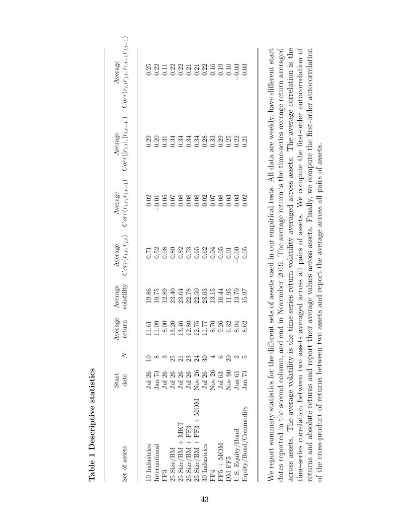
government bonds, and commodities. Table 1 presents descriptive statistics for each set of

15

assets. We report the start dates, the number of assets, the average across assets of the aver-

age returns, volatilities, and cross-correlations. Given that the ARPA methodology aims to

benefit from persistence in return moments, we also compute the first-order autocorrelation

coefficients of returns, absolute returns, and cross-products of returns. We average the first

two measures across all assets and the last across all pairs of assets. The first measure cap-

tures the persistence in the means, the second is a measure of the persistence in variances,

and the third measures persistence in covariances. All data are weekly, in USD, and end in

November 2019.

The first six sets of assets are those of DGU. The other sets contain either other equity risk

factors that have been proposed in the past decade or other asset classes. First, we consider

a set that contains ten value-weighted portfolios of U.S. stocks sorted by major industries.

The next set includes eight developed market equity indices: Canada, France, Germany,

Italy, Japan, Switzerland, U.K., and U.S. The next set includes the U.S. equity factors in

the Fama-French three-factor model (Fama and French, 1993); the value-weighted market

portfolio (MKT), the small-minus-big market capitalization factor (SMB), and the high-

minus-low book-to-market ratio factor (HML). The final sets of assets from DGU include

different combinations of 25 market capitalization and book-to-market ratio sorted value-

weighted U.S. stock portfolios with the previous three factors as well as the high-minus-low

previous 12-month return (skipping month t− 1) momentum factor (MOM, Jegadeesh and

Titman, 1993; Carhart, 1997). As in DGU, we remove from the sets 25 Size/BM + MKT,

25 Size/BM + FF3, and 25 Size/BM + FF3 + MOM the five portfolios with the largest

market capitalizations to prevent cases where assets would be too highly correlated.

The set 30 Industries contains 30 portfolios of U.S. stocks sorted by industry. We use

this set to measure the performance of the ARPA methodology when N is large, but the

portfolio sorting is not based on variables known to be related to expected returns like size

and book-to-market ratio. Next, we consider other sets of equity risk factors beyond the

Fama-French three-factor model. We first augment MKT, SMB, and HML with MOM.

16

Second, we use the Fama-French five-factor model with MKT, SMB, HML, a robust-minus-

weak profitability factor (RMW), a conservative-minus-aggressive investment factor (CMA)

that we augment with MOM. We also include a set DM FF5 that contains MKT, SMB,

RMW, CMA, and MOM for four regions (North America, Developed Europe, Japan, and

Asia Pacific).

Finally, we use two sets of assets that contain multiple asset classes. First, we combine

MKT and the 10-year U.S. government bond. Second, we use MKT, the 10-year U.S. gov-

ernment bond, the Datastream Developed Market ex North America index for international

stocks, the total return on the S&P Goldman Sachs Commodity Index, and the price of

gold. All U.S. equity data are obtained from Kenneth French’s website, the government

bond index from CRSP, and international stocks and commodity data from Datastream.

Our choice of sets of assets covers different investment styles. An investor may be in-

terested in the 10 Industries or 30 Industries set to try to generate outperformance by

rotating across defensive and aggressive industries during the business cycle. The different

combinations of market capitalization and book-to-market ratio sorted portfolios are used

by investors to benefit from the return predictability of these characteristics. The choice be-

tween using the 25 value-weighted portfolios or the long-short equity factors depends on the

investor’s ability to short-sell stocks. The set U.S. Equity/Bond considers the classic asset

allocation problem of how to optimally split a portfolio between stock market investments

and safer government bonds. Finally, the International and Equity/Bond/Commodity sets

represent other potential investment opportunity sets for both individual and institutional

investors.

U.S. equity data start in 1926 except for RMW and CMA, which start in 1963. The

U.S. government bond data start in 1961, the international equity indexes start in 1973, and

the developed market factor data start in 1990. Our sets cover both the case in which the

number of assets is small, for example, two for U.S. Equity/Bond and three for FF3, and as

large as 30 in the 30 Industries set. Recall that the parametric portfolio rule methodology of

17

Brandt et al. (2009) is difficult to implement in the former cases when the number of assets

is too small.

We next report the average returns and volatilities averaged across all assets in each

set. Sets with equity factors or bonds have lower returns and volatilities than sets with

equity portfolios. Portfolio diversification benefits are largely determined by correlations

between assets. We report in the sixth column the cross-correlation averaged across all pairs

of assets in each set. Cross-correlation for sets with equity factors and bonds range from

-0.05 to 0.08. Given these low correlations, simple combinations of these assets are bound

to generate substantial portfolio diversification benefits. In contrast, the other sets exhibit

higher than 0.52 average correlations. In such cases, optimally combining these assets into

portfolios is more challenging.

Average return autocorrelations are positive but small. None are higher than 0.08. In con-

trast, returns exhibit higher autocorrelations in absolute returns and return cross-products,

ranging from 0.21 to 0.34 and from -0.03 to 0.25, respectively. These averages suggest that

temporary deviations in portfolio allocations are more likely to be driven by time-variations

in the covariance matrix than in expected returns.

Overall, we consider sets of assets that mainly vary according to the number of assets and

their average cross-correlation. We next describe the two alternative portfolio allocations we

use to benchmark the ARPA portfolios.

3.2 Benchmark allocations

We use two portfolio rules to benchmark the ARPA. First, we follow DGU and use the

equal-weighted allocation as

wEWt,i (s, γ) =

1

N(s)∀i ∈ {1, ..., N(s)}.

18

where s is the set of assets. Note that this allocation does not depend on the risk aversion

γ and depends on s only through the number of assets N(s).

Second, we use the sample mean-variance estimator of wMarkowitzt as

wSMVt (s, γ) =

Σ−1t µt

γ

where Σt and µt are sample estimators of the covariance matrix and average excess returns,

respectively, using all past data (i.e., using returns from time 1 to t−1). In the next section,

we describe how we implement the out-of-sample portfolio allocation tests.

3.3 Out-of-sample tests

For each set of assets s and each risk aversion level γ, we determine a start date, TStart(s),

which corresponds to a quarter of the sample size (TStart(s) = ⌈T (s)/4⌉) or 10 years

(TStart(s) = 10 × 52), whichever is the largest. Then, each month t = TStart(s), TStart(s) +

1, ..., T (s) we follow these steps:

1. We estimate parameters using all past observations from the start of the sample period

to t − 1. We estimate Σt and µt to compute wSMVt (s, γ) and f , α, and β to obtain

wARPAt (s, γ).7 For the ARPA methodology, we re-estimate the parameters once a

year. While the parameter estimates are updated annually, the allocations are updated

weekly.

2. Following Ao et al. (2019), we compute the net of transaction cost performance for the

different portfolio rules as

rjp,t(s, γ) =

(1−

N∑i=1

ct,i|wjt,i(s, γ)− wj

t−,i(s, γ)|

)(1 + rf,t +

(wj

t (s, γ))′rt

)− 1,

where j = EW,SMV,ARPA and ct,i is a cost level that measures the transaction cost7We omit the dependence of Σt and µt on s and of f , α, and β on s and γ to lighten the notation.

19

per dollar traded for trading asset i and wjt−,i(s, γ) is the portfolio weight for asset i at

the beginning of period t before rebalancing. For simplicity, we set ct,i = 0.5% for all

t and i. Transaction costs affect the realized performance of all strategies. But most

importantly, they affect the estimation of the ARPA model. Indeed, the numerical

optimization of the UMVC to estimate f , α, and β takes into account transaction

costs when computing the UMVC. For example, a higher α value is chosen only if it

brings enough performance benefits to counteract the increased turnover.

At the end of November 2019, we compute the realized UMVCs as

UMV Cj(s, γ) = E[rjp,t(s, γ)]−γ

2V ar[rjp,t(s, γ)] (11)

where the sample average return E and sample return variance V ar are computed using

portfolio j’s returns from t = TStart(s) to t = T (s). Finally, we consider investors with

different levels of risk aversion γ ∈ {1, 3, 5, 10} and with different allocation constraints

(unconstrained or with no short-selling and full-investment constraints). We present the out-

of-sample results for the unconstrained investor in the next section and analyze contrained

allocations in Section 3.7.

3.4 Out-of-sample performance for unconstrained portfolios

We first focus on unconstrained investors. This case is usually challenging because the

Markowitz portfolio rule is known to maximize estimation errors, see Michaud (1989). There-

fore, unconstrained optimized portfolio allocations typically result in large infeasible weights

and poor out-of-sample performances.

Table 2 contains our main results. We report the realized unconditional mean-variance

criteria in percent per year for the EW, SMV, and ARPA portfolios for all risk aversion

levels. We bootstrap the realized time series of portfolio returns to assess the significance of

the difference in UMVCs between the SMV and the EW portfolios and between the ARPA

20

and the EW portfolios.8

First, the UMVCs across risk aversion levels for the SMV portfolios are more often than

not lower than the UMVCs for the EW portfolio. Even worse, they are, in some cases,

negative; the SMV portfolio destroys value on a risk-adjusted basis. These results echo the

findings of DGU. They are more often negative for the most risk-seeking investor with γ = 1.

In sharp contrast, the ARPA portfolio outperforms the EW portfolio for all but two

sets containing equity factors or size and book-to-market ratio sorted portfolio: FF3, 25

Size/BM, 25 Size/BM + MKT, 25 Size/BM + FF3, 25 Size/BM + FF3 + MOM, FF4, FF5

+ MOM, DM FF5. The outperformances are statistically significant, except in a few cases

when risk aversion is high. The outperformances for the set DM FF5 are not significant,

despite their economic magnitude, because of the short sample period.

The industry portfolios and international equity portfolios significantly outperform when

risk aversion is high. The performance for multi-asset class sets is lower than for the EW

portfolio. Finally, in all cases, when the SMV significantly outperforms the EW portfolio,

we find that the ARPA portfolio further outperforms. This result indicates the benefit of

the dynamic portfolio rebalancing modeled in the ARPA methodology.

On average across all sets of assets and risk aversion levels, the proportional increase in

realized UMVCs going from the EW to the ARPA portfolio is more than 100% (unreported).

However, there are important differences across sets of assets and risk aversion levels. There-

fore, to gain a better perspective on these differences, we further explore the determinants

of outperformance in the next section.

3.5 Under which conditions does ARPA outperform?

In this section, we run panel regressions to better understand under which conditions do

ARPA portfolios outperform the EW benchmark. Precisely, we investigate the determinants

of the contribution to performance for each week t, each asset set s, and each risk aversion8We create 10,000 bootstrap samples. We also used the block bootstrap of Politis and Romano (1994)

and find similar results.

21

γ defined as,

UMV CARPAt (s, γ) = rARPA

p,t (s, γ)− γ

2

(rARPAp,t (s, γ)− E[rARPA

p,t (s, γ)])2

. (12)

In this equation, rARPAp,t (s, γ) is the return at time t for the ARPA portfolio for asset set s

and risk aversion level γ. The realized mean-variance criteria, UMV CARPA(s, γ), defined in

Equation (11) and reported in Table 2 are the time-series averages of UMV CARPAt (s, γ).

We similarly compute the performance contributions, UMV CEWt (s, γ), for the EW port-

folios. Then, we compute the relative difference as

∆UMV CARPA−EWt (s, γ) =

UMV CARPAt (s, γ)− UMV CEW

t (s, γ)

|UMV CEW (s, γ)|. (13)

In this equation, we compute the difference in performance contribution between the ARPA

and EW portfolio at time t, and standardize it by the realized UMVC of the EW portfolio,

UMV CEW (s, γ). We use the absolute value of the denominator to preserve the direction of

the outperformance in the one case where the UMV CEW (s, γ) is negative.

We use the analysis of DGU to guide our empirical investigation of the determinants

of ARPA’s outperformance relative to EW. They analytically show that the sample-based

optimal mean-variance allocation (i.e., the SMV portfolio) is expected to outperform the

equal-weighted allocation if three conditions are met: (i) the estimation sample is long

enough, (ii) the number of assets is small enough, and (iii) the ex ante squared Sharpe

ratio of the optimized portfolio is substantially higher than the one for the EW portfolio.

Condition (i) is explained by the need to have a large enough sample of returns to estimate

return moments and condition (ii) implies that the number of return moments to estimate

should not be too large relative to the sample size. Condition (iii) states that there should

be a benefit for optimizing allocations relative to using an equally weighted allocation.

We run the following panel regression for the performance contribution of the ARPA

22

portfolio relative to the EW portfolio on different explanatory variables,

∆UMV CARPA−EWt (s, γ) = κ+Xt,s,γβ + ϵt,s,γ, (14)

where κ is a constant, Xt,s,γ is a vector of explanatory variables, β is a vector of coefficients,

and ϵt,s,γ are error terms. All regressors are demeaned and standardized by their respective

range such that the estimated constant is the average relative outperformance across all

asset sets and risk aversion levels. We combine observations for all weeks, asset sets, and

risk aversion levels, resulting in 153, 524 observations. We cluster standard errors by asset

set.

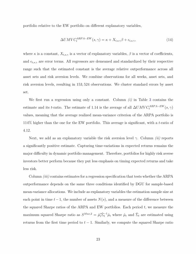
We first run a regression using only a constant. Column (i) in Table 3 contains the

estimate and its t-ratio. The estimate of 1.14 is the average of all ∆UMV CARPA−EWt (s, γ)

values, meaning that the average realized mean-variance criterion of the ARPA portfolio is

114% higher than the one for the EW portfolio. This average is significant, with a t-ratio of

4.12.

Next, we add as an explanatory variable the risk aversion level γ. Column (ii) reports

a significantly positive estimate. Capturing time-variations in expected returns remains the

major difficulty in dynamic portfolio management. Therefore, portfolios for highly risk averse

investors better perform because they put less emphasis on timing expected returns and take

less risk.

Column (iii) contains estimates for a regression specification that tests whether the ARPA

outperformance depends on the same three conditions identified by DGU for sample-based

mean-variance allocations. We include as explanatory variables the estimation sample size at

each point in time t− 1, the number of assets N(s), and a measure of the difference between

the squared Sharpe ratios of the ARPA and EW portfolios. Each period t, we measure the

maximum squared Sharpe ratio as SMax,2 = µ′tΣ

−1t µt where µt and Σt are estimated using

returns from the first time period to t− 1. Similarly, we compute the squared Sharpe ratio

23

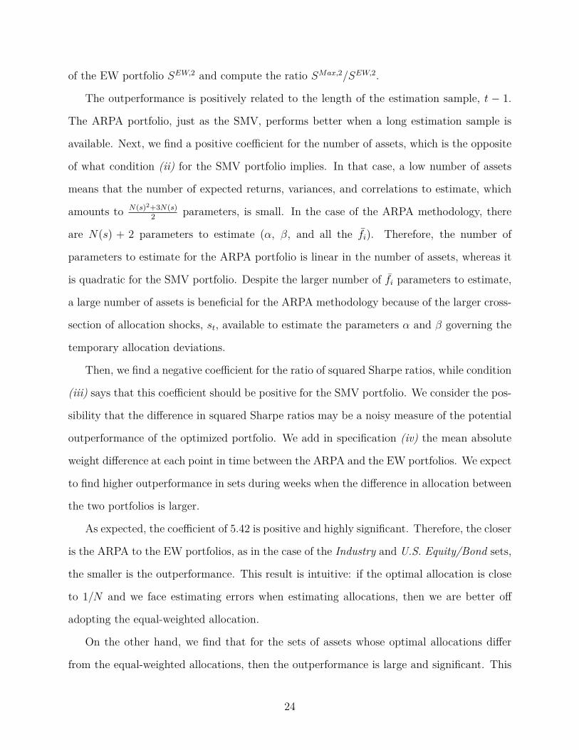
of the EW portfolio SEW,2 and compute the ratio SMax,2/SEW,2.

The outperformance is positively related to the length of the estimation sample, t − 1.

The ARPA portfolio, just as the SMV, performs better when a long estimation sample is

available. Next, we find a positive coefficient for the number of assets, which is the opposite

of what condition (ii) for the SMV portfolio implies. In that case, a low number of assets

means that the number of expected returns, variances, and correlations to estimate, which

amounts to N(s)2+3N(s)2

parameters, is small. In the case of the ARPA methodology, there

are N(s) + 2 parameters to estimate (α, β, and all the fi). Therefore, the number of

parameters to estimate for the ARPA portfolio is linear in the number of assets, whereas it

is quadratic for the SMV portfolio. Despite the larger number of fi parameters to estimate,

a large number of assets is beneficial for the ARPA methodology because of the larger cross-

section of allocation shocks, st, available to estimate the parameters α and β governing the

temporary allocation deviations.

Then, we find a negative coefficient for the ratio of squared Sharpe ratios, while condition

(iii) says that this coefficient should be positive for the SMV portfolio. We consider the pos-

sibility that the difference in squared Sharpe ratios may be a noisy measure of the potential

outperformance of the optimized portfolio. We add in specification (iv) the mean absolute

weight difference at each point in time between the ARPA and the EW portfolios. We expect

to find higher outperformance in sets during weeks when the difference in allocation between

the two portfolios is larger.

As expected, the coefficient of 5.42 is positive and highly significant. Therefore, the closer

is the ARPA to the EW portfolios, as in the case of the Industry and U.S. Equity/Bond sets,

the smaller is the outperformance. This result is intuitive: if the optimal allocation is close

to 1/N and we face estimating errors when estimating allocations, then we are better off

adopting the equal-weighted allocation.

On the other hand, we find that for the sets of assets whose optimal allocations differ

from the equal-weighted allocations, then the outperformance is large and significant. This

24

result is not mechanical; we could have obtained different portfolio allocations and poorer

performance, as in the case of the SMV portfolio.

The definition of the performance contribution UMV CARPAt (s, γ) in Equation (12) uses

the sample average portfolio return computed using all returns in the contribution to realized

portfolio variance. To ensure that this use of forward-looking information does not impact

our results, we also run the panel regressions with UMV CARPAt (s, γ) computed with the

average portfolio return up to time t− 1. All the results are virtually unchanged.

Overall, we find that the ARPA methodology provides benefits in out-of-sample portfolio

performances, especially when optimal allocations differ from the equal-weighted portfolio.

In the next section, we examine the dynamics of the estimated ARPA parameters and allo-

cations.

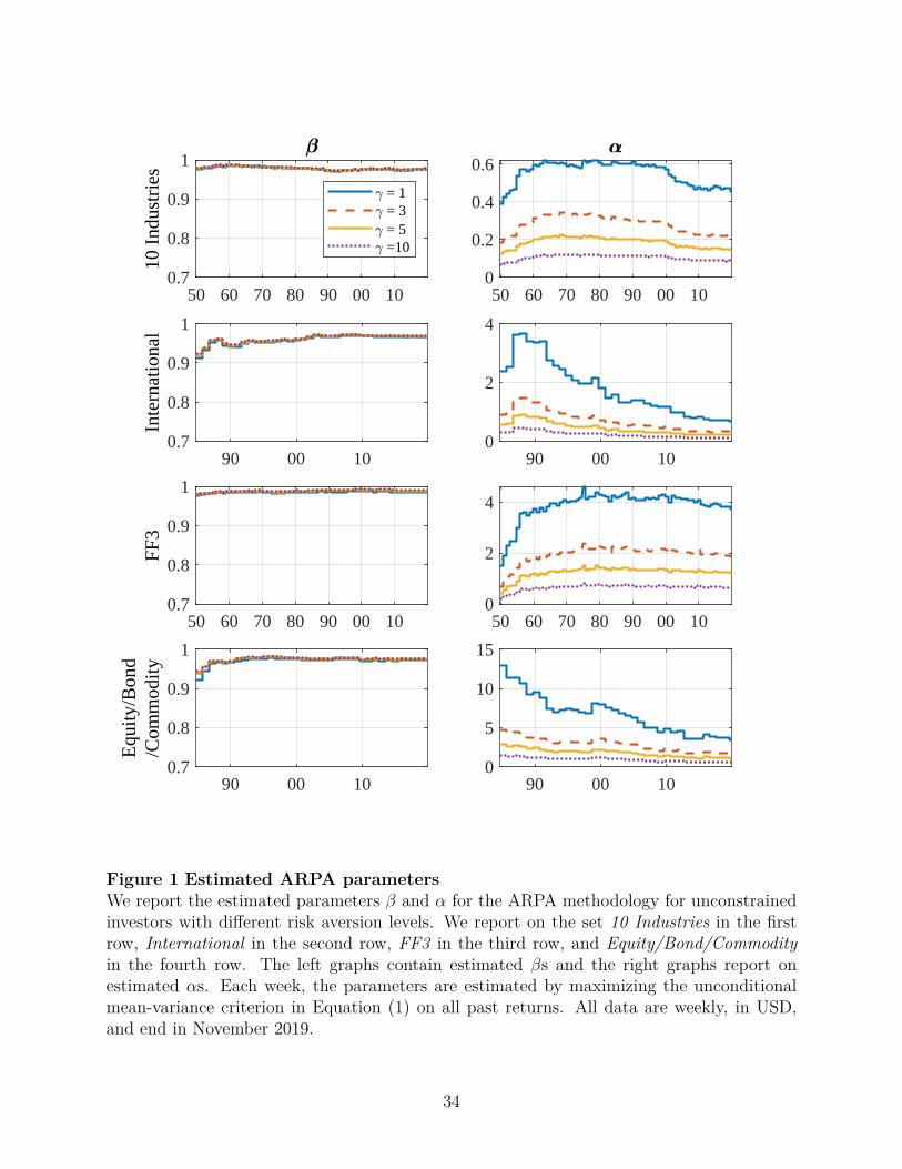
3.6 How do β and α vary?

To gain more intuition on the ARPA results, we examine in this section the dynamics of the

estimated parameters and the dynamic portfolio allocations.

To save space, we focus our discussion on four representative sets of assets: 10 Indus-

tries, International, FF3, and Equity/Bond/Commodity.9 Figure 1 reports the time-series of

estimated α and β parameters for all risk aversion levels. Recall that these parameters are

estimated each week using all past returns.

The β parameters are all above 0.9 and they do not differ across risk aversion levels.

These high values indicate that deviations from the strategic asset allocations are highly

persistent.

Differently, the α parameters reported in the right graphs vary between sets of assets.

They go up to 0.6 for 10 Industries, up to 4 for International and FF3, and up to 15 for

Equity/Bond/Commodity. The αs also consistently vary across risk aversion levels. The

lower the risk aversion, the higher is the estimated α. However, these higher α values do not9All results are available from the author.

25

necessarily imply that the risk tolerant investor trades more. Instead, they are indicative of

the larger scales of the latent variables, ft, and allocation shocks, st, for investors with low

risk aversion.

To see this point more clearly, Figures 2 to 5 respectively report for each set of assets

the dynamic allocations over time. First, we see in Figures 4 for the set FF3 the sources of

outperformance of the ARPA versus the EW portfolio. All investors, except the most risk

averse one, take on leverage to generate outperformance. Further, they allocate consistently

to the MKT and HML factors, and very little to the SMB factors, whereas the EW portfolio

is constantly invested in the SMB factor with a 33.33% allocation.

All dynamic allocations show a small number of short positions and persistent allocations

to some assets. Across all sets, we unsurprisingly find that portfolio leverage decreases as

risk aversion increases.

In summary, we obtain better out-of-sample performance for unconstrained portfolios

using the ARPA methodology. The generated outperformance is obtained by adopting per-

sistent leveraged long and small short positions. In the next section, we consider the case of

a constrained investor who cannot short sell and is fully invested in risky assets, constraints

similar to those of a mutual fund.

3.7 Out-of-sample performance for constrained portfolios

We report in Table 4 the realized unconditional mean-variance criterion for the ARPA port-

folios in which we constrain allocations to be non-negative and to sum to one. We compare

their performance to the EW and constrained SMV portfolios. The constrained SMV port-

folio is found by numerically optimizing the historical mean-variance criterion using constant

non-negative allocations that sum to one.

We find that the ARPA portfolio outperforms the EW portfolio for the same sets of

assets as for the unconstrained investors, but less so when risk aversion is high. Unsurpris-

ingly, the magnitude of the outperformance is smaller for constrained allocations than for

26

unconstrained allocations in Table 2.

The constrained SMV portfolio performs better than the unconstrained SMV portfolio,

in line with the findings of Jagannathan and Ma (2003). In several cases, the ARPA does

not outperform the constrained SMV portfolio. Therefore, the ARPA methodology is more

effective at delivering outperformance when the portfolio allocations are not constrained.

To gain a better perspective on these results, we estimate the panel regression in Equation

(14) using the performance contributions of the constrained portfolios as the left-hand-side

variable. The results are presented in Table 5.

The average outperformance across all asset sets and risk aversion levels is 0.25 and is

always significant at the 1% level. Therefore, even in the case with allocation constraints,

the ARPA methodology significantly increases the realized UMVC compared to the EW

portfolio. While the improvement was more than 100% in the unconstrained case, it is 25%

in the constrained case.

We find as in the unconstrained case that outperformance is positively related to the risk

aversion level, the length of the estimation sample, the number of assets, and the weekly

average allocation difference between the ARPA and EW portfolios, although the last two

coefficients are not significant.

In contrast to the unconstrained case, we find that outperformance of the constrained

portfolio is positively related to the squared Sharpe ratio difference. This result is in line

with DGU’s condition (iii) for the outperformance of the SMV versus the EW portfolio.

Overall, the results in Table 5 are consistent with those in Table 3. The notable excep-

tion is that the unconstrained outperformance is significantly related to average allocation

difference, whereas the constrained outperformance is significantly related to the ratio of

squared Sharpe ratios.

Finally, Figures 6-9 present the allocations over time for the sets 10 Industries, Inter-

national, FF3, and Equity/Bond/Commodity.Allocations significantly vary over time and

across risk aversion levels. Consider the set FF3 for example, the investor with a low risk

27

aversion (γ = 1) is almost always invested in the market portfolio to achieve higher average

return and risk, whereas the investor with a high risk aversion (γ = 10) adopts a more

balanced allocation across MKT, SMB, and HML.

4 Conclusion

We provide a new methodology to model dynamic mean-variance portfolio allocations to op-

timize an unconditional mean-variance criterion. We parameterize portfolio allocations using

an auto-regressive process in which the shock is the gradient of the investor’s realized mean-

variance criterion with respect to portfolio allocation. Our methodology handles transaction

costs, allocation constraints, and can be used even if there are no instruments available

to model time-variations in portfolio allocations. Given these features, our methodology

significantly contributes to the literature on parametric portfolio rules.

We run empirical tests using equity portfolios, equity long-short factors, government

bonds, and commodities. We find that our methodology outperforms benchmark portfolio

rules.

The time-series approach we use to model portfolio allocations makes it possible to extend

our methodology in different directions. In Equation (6), α and β are scalar parameters.

Hence, we restrict the persistence in ft to be the same for all assets and preclude cross-asset

effects in which the lagged shock for one asset could impact the current weight for another

asset. We can generalize the auto-regressive process for portfolio allocations to use more

general parameter matrices to account for asset-specific weight persistence and cross-asset

effects.

Also, we can include a set of characteristics Xt on the right-hand side of the allocation

dynamic to nest the BSV approach and empirically evaluate the value of our allocation shock

compared to other instruments used in the literature. We leave these points for further

research.

28

A Allocation constraints and associated gradients

We considered in our main results, an unconstrained investor and an investor constrained to

have positive allocations and be fully invested in risky assets. In this appendix, we provide

the portfolio allocation shocks for other allocation constraints: the case with only a no

short-selling constraint and the case with only the constraint that allocations sum to one.

A.1 No short-sales

We use the function W (ft) = eft to prevent short-sales. The portfolio allocation shocks are

then

st =1

Tdiag(eft) (rt − γ (rp,t − rp) rt) . (15)

The effect of the adjustment eft is the following. If ft,i is a small number, then eft,i is close

to zero. In such case, there is no shock to the allocation of asset i and ft+1,i reverts back up

to fi because of the term βft,i in Equation (6). Therefore, randomness is shut down when

the allocation of an asset gets close to 0.

A.2 Fully invested in risky assets

We use the function W (ft) =ft∑N

j=1 ft,jto ensure weights sum to 1. The portfolio allocation

shocks are then

st =1

T

(IN −W (ft)ι

′N∑N

j=1 ft,j

)′

(rt − γ (rp,t − rp) rt) , (16)

where ιN is a N -by-ones vector of ones.

29

References

Ait-Sahalia, Y., and M. W. Brandt. 2001. Variable selection for portfolio choice. Journal of

Finance 56:1297–1351.

Anderson, E. W., and A.-R. Cheng. 2016. Robust bayesian portfolio choices. Review of

Financial Studies 29:1330–1375.

Ao, M., Y. Li, and X. Zheng. 2019. Approaching mean-variance efficiency for large portfolios.

Review of Financial Studies 32:2890–2919.

Barroso, P., and P. Santa-Clara. 2015. Beyond the carry trade: optimal currency portfolios.

Journal of Financial and Quantitative Analysis 50:1037–1056.

Basak, S., and G. Chabakauri. 2010. Dynamic mean-variance asset allocation. Review of

Financial Studies 23:2970–3016.

Bollerslev, T., B. Hood, J. Huss, and L. H. Pedersen. 2018. Risk everywhere: modeling and

managing volatility. Review of Financial Studies 31:2729–2773.

Brandt, M. W. 1999. Estimating portfolio and consumption choice: a conditional Euler

equations approach. Journal of Finance 54:1609–1645.

Brandt, M. W. 2010. Handbook of Financial Econometrics, vol. Volume 1: Tools and Tech-

niques, chap. Portfolio Choice Problems. North Holland.

Brandt, M. W., and P. Santa-Clara. 2006. Dynamic portfolio selection by augmenting the

asset space. Journal of Finance 61:2187–2218.

Brandt, M. W., P. Santa-Clara, and R. Valkanov. 2009. Parametric portfolio policies: ex-

ploiting characteristics in the cross-section of equity returns. Review of Financial Studies

22:3411–3447.

30

Bredendiek, M., G. Ottonello, and R. Valkanov. 2019. Corporate Bond Portfolios and Asset-

Specific Information. Working paper, UCSD .

Carhart, M. M. 1997. On Persistence in Mutual Fund Performance. Journal of Finance

52:57–82.

Cochrane, J. H. 2014. A mean-variance benchmark for intertemporal portfolio theory. Jour-

nal of Finance 69:1–49.

Creal, D., S. J. Koopman, and A. Lucas. 2011. A dynamic multivariate heavy-tailed model

for time-varying volatilities and correlations. Journal of Business & Economic Statistics

29:552–563.

DeMiguel, V., L. Garlappi, F. J. Nogales, and R. Uppal. 2009a. A generalized approach to

portfolio optimization: Improving performance by constraining portfolio norms. Manage-

ment Science 55:798–812.

DeMiguel, V., L. Garlappi, and R. Uppal. 2009b. Optimal versus naive diversification: how

inefficient is the 1/N portfolio strategy? Review of Financial Studies 22:1915–1953.

DeMiguel, V., A. M. Utrera, F. J. Nogales, and R. Uppal. 2019. A portfolio perspective on

the multitude of firm characteristics. Forthcoming in the Review of Financial Studies .

Engle, R. F., O. Ledoit, and M. Wolf. 2019. Large dynamic covariance matrices. Journal of

Business & Economic Statistics 37:363–375.

Fama, E. F., and K. R. French. 1993. Common risk factors in the returns on stocks and

bonds. Journal of Financial Economics 33:3–56.

Ferson, W. E., and A. F. Siegel. 2001. The efficient use of conditioning information in

portfolios. Journal of Finance 56:967–982.

Ferson, W. E., and A. F. Siegel. 2009. Testing portfolio efficiency with conditioning infor-

mation. Review of Financial Studies 22:2535–2558.

31

Fleming, J., C. Kirby, and B. Ostdiek. 2001. The economic value of volatility timing. Journal

of Finance 56:329–352.

Fleming, J., C. Kirby, and B. Ostdiek. 2003. The economic value of volatility timing using

”realized” volatility. Journal of Financial Economics 67:473–509.

Gârleanu, N., and L. H. Pedersen. 2013. Dynamic trading with predictable returns and

transaction costs. Journal of Finance 68:2309–2340.

Ghysels, E., A. Plazzi, and R. Valkanov. 2016. Why invest in emerging markets? The role

of conditional return asymmetry. Journal of Finance 71:2145–2192.

Gu, S., B. T. Kelly, and D. Xiu. 2019. Empirical asset pricing via machine learning. Forth-

coming in the Review of Financial Studies .

Jagannathan, R., and T. Ma. 2003. Risk reduction in large portfolios: why imposing the

wrong constraints helps. Journal of Finance 58:1651–1683.

Jegadeesh, N., and S. Titman. 1993. Returns to Buying Winners and Selling Losers: Impli-

cations for Stock Market Efficiency. Journal of Finance 48:65–91.

Kan, R., and G. Zhou. 2007. Optimal portfolio choice with parameter uncertainty. Journal

of Financial and Quantitative Analysis 42:621–656.

Kirby, C., and B. Ostdiek. 2012a. It’s all in the timing: simple active portfolio strategies

that outperform naıve diversification. Journal of Financial and Quantitative Analysis

47:437–467.

Kirby, C., and B. Ostdiek. 2012b. Optimizing the performance of sample mean-variance

efficient portfolios. Working paper, UNC and Rice University .

Lucas, A., B. Schwaab, and X. Zhang. 2014. Conditional Euro Area Sovereign Default Risk.

Journal of Business & Economic Statistics 32:271–284.

32

Markowitz, H. M. 1952. Portfolio selection. Journal of Finance 7:77–91.

Marquering, W., and M. Verbeek. 2004. The economic value of predicting stock index returns

and volatility. Journal of Financial and Quantitative Analysis 39:407–429.

Michaud, R. O. 1989. The Markowitz optimization enigma: is ”optimized” optimal? Finan-

cial Analyst Journal 45:31–42.

Politis, D. N., and J. P. Romano. 1994. The stationary bootstrap. Journal of the American

Statistical Association 89:1303–1313.

Raponi, V., R. Uppal, and P. Zaffaroni. 2020. Robust portfolio choice. Working paper,

EDHEC .

Tu, J., and G. Zhou. 2011. Markowitz meets Talmud: A combination of sophisticated and

naive diversification strategies. Journal of Financial Economics 99:204–215.

Uppal, R., P. Zaffaroni, and I. Zviadadze. 2020. Correcting misspecified stochastic discount

factors. Working paper, EDHEC .

33

50 60 70 80 90 00 100

0.2

0.4

0.6

50 60 70 80 90 00 100.7

0.8

0.9

110

Ind

ustr

ies

= 1 = 3 = 5 =10

90 00 100

2

4

90 00 100.7

0.8

0.9

1

Inte

rnat

iona

l

50 60 70 80 90 00 100

2

4

50 60 70 80 90 00 100.7

0.8

0.9

1

FF3

90 00 100

5

10

15

90 00 100.7

0.8

0.9

1

Equ

ity/B

ond

/Com

mod

ity

Figure 1 Estimated ARPA parametersWe report the estimated parameters β and α for the ARPA methodology for unconstrainedinvestors with different risk aversion levels. We report on the set 10 Industries in the firstrow, International in the second row, FF3 in the third row, and Equity/Bond/Commodityin the fourth row. The left graphs contain estimated βs and the right graphs report onestimated αs. Each week, the parameters are estimated by maximizing the unconditionalmean-variance criterion in Equation (1) on all past returns. All data are weekly, in USD,and end in November 2019.

34

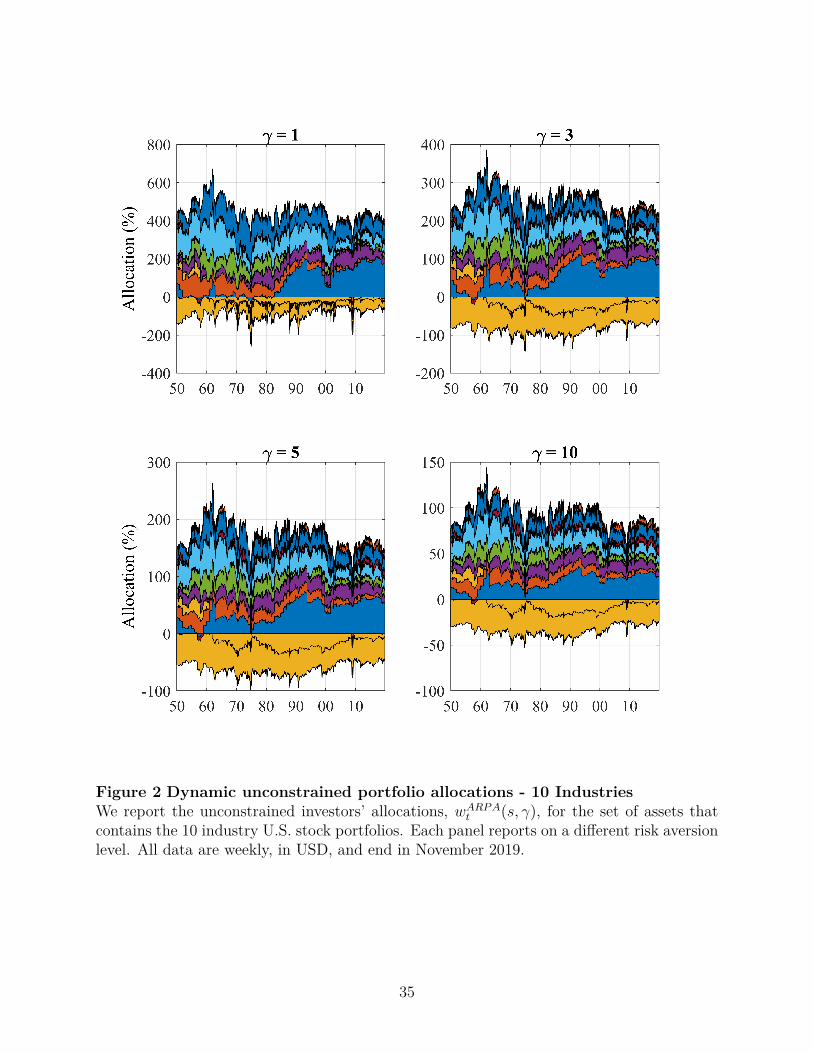
Figure 2 Dynamic unconstrained portfolio allocations - 10 IndustriesWe report the unconstrained investors’ allocations, wARPA

t (s, γ), for the set of assets thatcontains the 10 industry U.S. stock portfolios. Each panel reports on a different risk aversionlevel. All data are weekly, in USD, and end in November 2019.

35

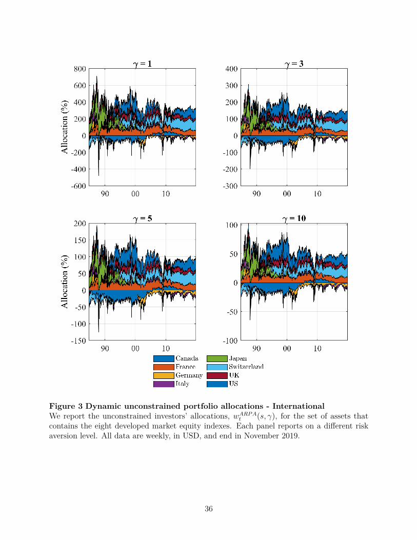
Figure 3 Dynamic unconstrained portfolio allocations - InternationalWe report the unconstrained investors’ allocations, wARPA

t (s, γ), for the set of assets thatcontains the eight developed market equity indexes. Each panel reports on a different riskaversion level. All data are weekly, in USD, and end in November 2019.

36

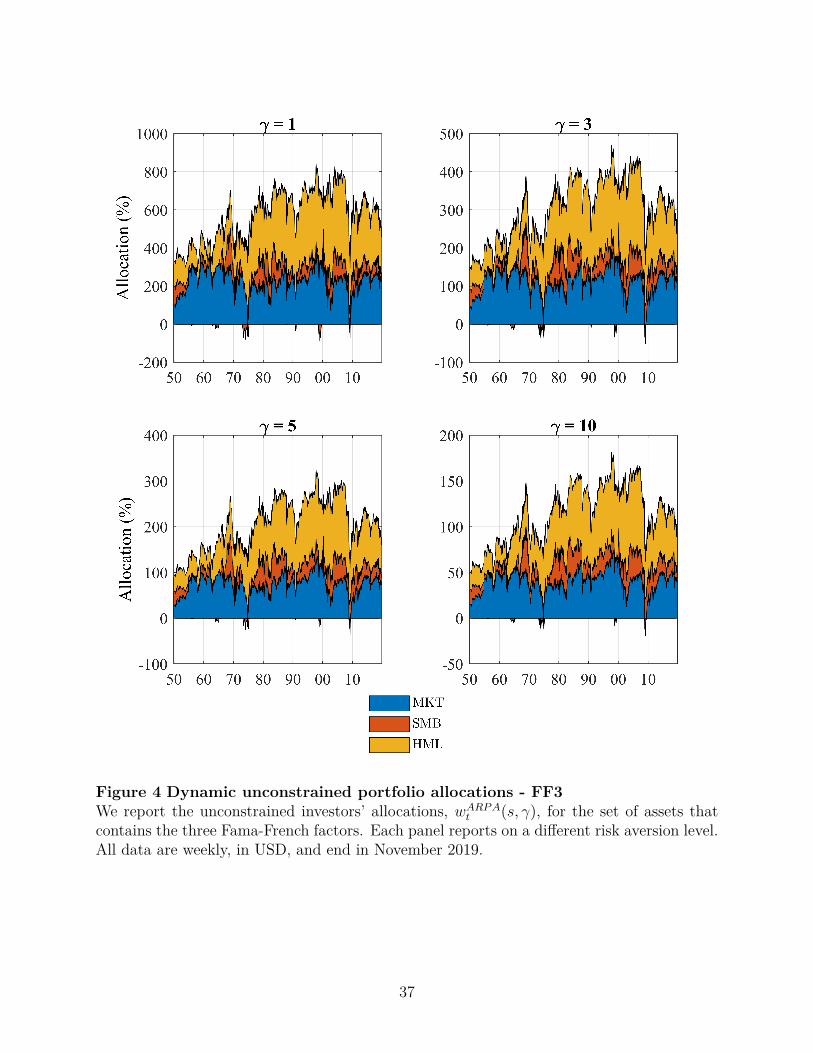
Figure 4 Dynamic unconstrained portfolio allocations - FF3We report the unconstrained investors’ allocations, wARPA

t (s, γ), for the set of assets thatcontains the three Fama-French factors. Each panel reports on a different risk aversion level.All data are weekly, in USD, and end in November 2019.

37

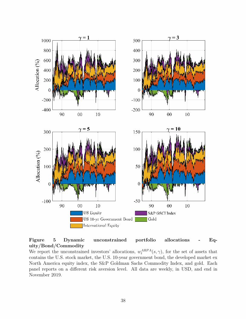
Figure 5 Dynamic unconstrained portfolio allocations - Eq-uity/Bond/CommodityWe report the unconstrained investors’ allocations, wARPA

t (s, γ), for the set of assets thatcontains the U.S. stock market, the U.S. 10-year government bond, the developed market exNorth America equity index, the S&P Goldman Sachs Commodity Index, and gold. Eachpanel reports on a different risk aversion level. All data are weekly, in USD, and end inNovember 2019.

38

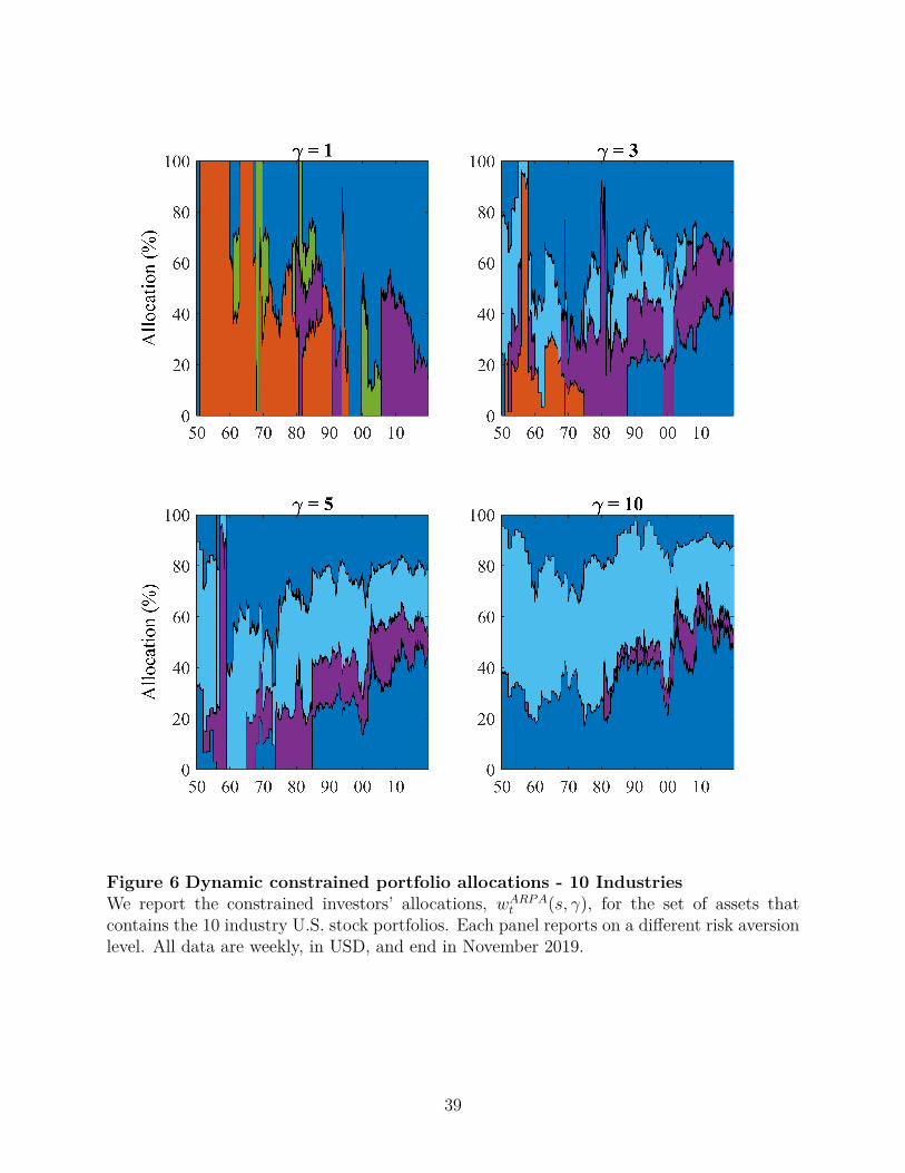
Figure 6 Dynamic constrained portfolio allocations - 10 IndustriesWe report the constrained investors’ allocations, wARPA

t (s, γ), for the set of assets thatcontains the 10 industry U.S. stock portfolios. Each panel reports on a different risk aversionlevel. All data are weekly, in USD, and end in November 2019.

39

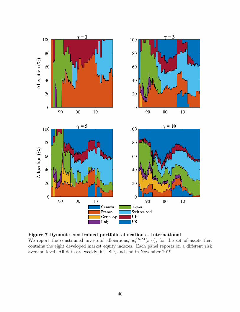
Figure 7 Dynamic constrained portfolio allocations - InternationalWe report the constrained investors’ allocations, wARPA

t (s, γ), for the set of assets thatcontains the eight developed market equity indexes. Each panel reports on a different riskaversion level. All data are weekly, in USD, and end in November 2019.

40

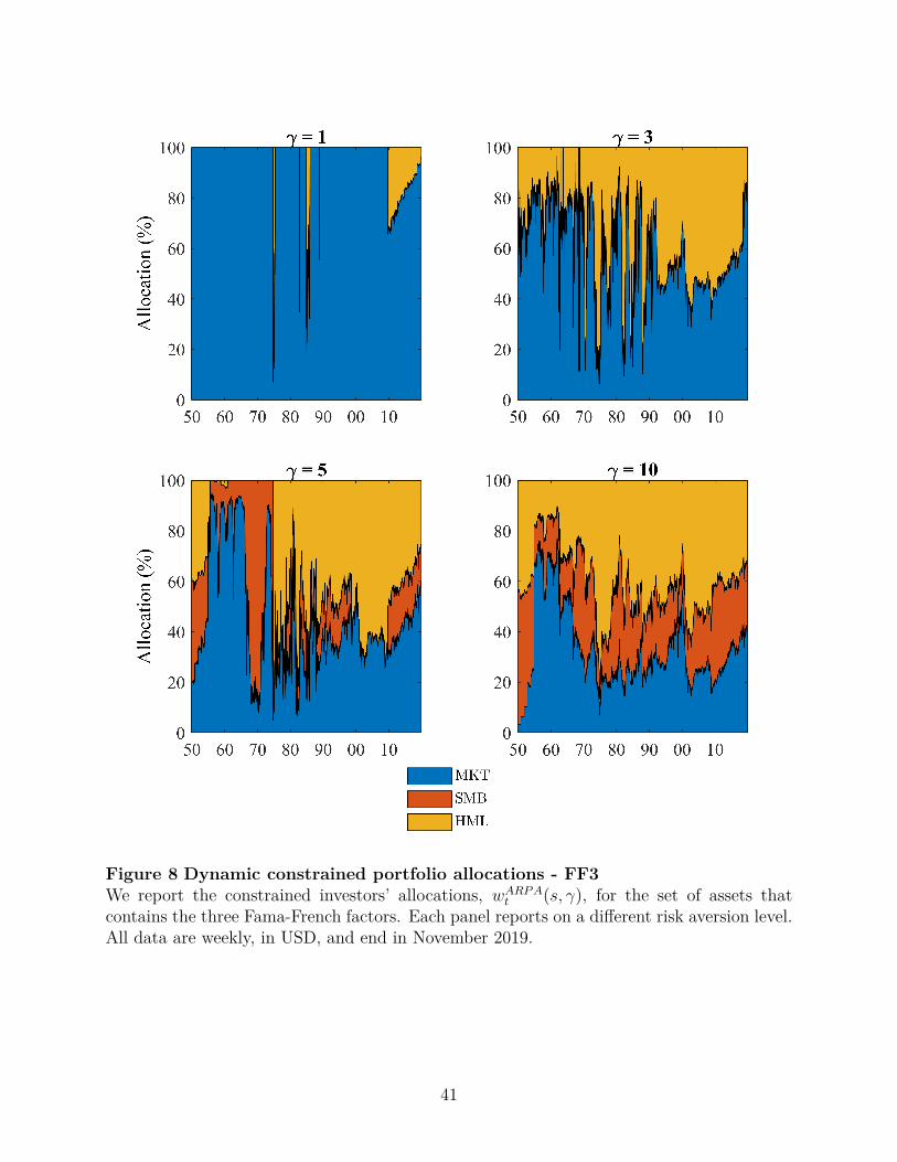
Figure 8 Dynamic constrained portfolio allocations - FF3We report the constrained investors’ allocations, wARPA

t (s, γ), for the set of assets thatcontains the three Fama-French factors. Each panel reports on a different risk aversion level.All data are weekly, in USD, and end in November 2019.

41

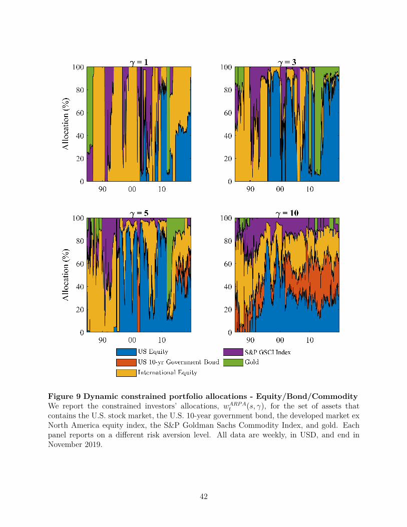
Figure 9 Dynamic constrained portfolio allocations - Equity/Bond/CommodityWe report the constrained investors’ allocations, wARPA

t (s, γ), for the set of assets thatcontains the U.S. stock market, the U.S. 10-year government bond, the developed market exNorth America equity index, the S&P Goldman Sachs Commodity Index, and gold. Eachpanel reports on a different risk aversion level. All data are weekly, in USD, and end inNovember 2019.

42

Tabl

e1

Des

crip

tive

stat

isti

cs

Star

tAv

erag

eAv

erag

eAv

erag

eAv

erag

eAv

erag

eAv

erag

eSe

tof

asse

tsda

teN

retu

rnvo

latil

ityCorr(r i

,t,r

j,t)

Corr(r i

,t,r

i,t−

1)

Corr(|r

i,t|,|r

i,t−

1|)

Corr(r i

,tr j

,t,r

i,t−

1r j

,t−1)

10In

dust

ries

Jul2

610

11.61

19.86

0.71

0.02

0.29

0.25

Inte

rnat

iona

lJa

n73

811

.09

19.75

0.52

−0.01

0.20

0.22

FF3

Jul2

63

8.00

12.89

0.08

0.05

0.31

0.11

25Si

ze/B

MJu

l26

2513

.20

23.40

0.80

0.07

0.34

0.22

25Si

ze/B

M+

MK

TJu

l26

2113

.46

23.64

0.82

0.08

0.34

0.22

25Si

ze/B

M+

FF3

Jul2

623

12.80

22.78

0.73

0.08

0.34

0.21

25Si

ze/B

M+

FF3

+M

OM

Nov

2624

12.75

22.50

0.65

0.08

0.34

0.21

30In

dust

ries

Jul2

630

11.77

23.03

0.62

0.02

0.28

0.22

FF4

Nov

264

8.70

13.15

−0.04

0.07

0.33

0.16

FF5

+M

OM

Jul6

36

9.26

10.44

−0.05

0.08

0.29

0.19

DM

FF5

Nov

9020

6.32

11.95

0.01

0.03

0.25

0.10

U.S

.Equ

ity/B

ond

Jun

612

8.04

13.70

−0.00

0.03

0.22

−0.03

Equi

ty/B

ond/

Com

mod

ityJa

n73

58.62

15.97

0.05

0.02

0.21

0.03

We

repo

rtsu

mm

ary

stat

istic

sfor

the

diffe

rent

sets

ofas

sets

used

inou

rem

piric

alte

sts.

All

data

are

week

ly,h

ave

diffe

rent

star

tda

tesr

epor

ted

inth

ese

cond

colu

mn,

and

end

inN

ovem

ber2

019.

The

aver

age

retu

rnis

the

time-

serie

save

rage

retu

rnav

erag

edac

ross

asse

ts.

The

aver

age

vola

tility

isth

etim

e-se

ries

retu

rnvo

latil

ityav

erag

edac

ross

asse

ts.

The

aver

age

corr

elat

ion

isth

etim

e-se

ries

corr

elat

ion

betw

een

two

asse

tsav

erag

edac

ross

allp

airs

ofas

sets

.W

eco

mpu

teth

efir

st-o

rder

auto

corr

elat

ion

ofre

turn

san

dab

solu

tere

turn

san

dre

port

thei

rav

erag

eva

lues

acro

ssas

sets

.Fi

nally

,we

com

pute

the

first

-ord

erau

toco

rrel

atio

nof

the

cros

s-pr

oduc

tof

retu

rns

betw

een

two

asse

tsan

dre

port

the

aver

age

acro

ssal

lpai

rsof

asse

ts.

43

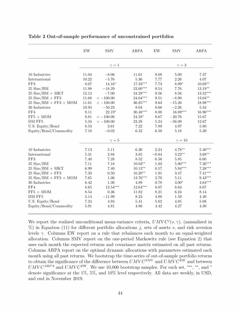
Table 2 Out-of-sample performance of unconstrained portfolios

EW SMV ARPA EW SMV ARPA

γ = 1 γ = 3

10 Industries 11.04 −8.06 11.61 9.08 5.00 7.37International 10.22 −5.76 5.36 7.77 2.26 4.07FF3 8.07 14.16∗ 17.33∗∗∗ 7.73 8.99∗ 10.69∗∗

25 Size/BM 11.98 −18.29 23.00∗∗∗ 9.54 7.76 13.19∗∗

25 Size/BM + MKT 12.12 −7.00 24.28∗∗∗ 9.56 8.56 13.52∗∗∗

25 Size/BM + FF3 11.68 < −100.00 24.04∗∗∗ 9.51 −8.90 13.04∗∗

25 Size/BM + FF3 + MOM 11.61 < −100.00 36.85∗∗∗ 9.63 −15.26 18.98∗∗∗

30 Industries 10.94 −50.23 8.04 8.68 −2.26 5.34FF4 9.11 22.19∗ 30.48∗∗∗ 8.88 16.89∗∗∗ 16.96∗∗∗

FF5 + MOM 8.81 < −100.00 24.58∗ 8.67 −20.76 15.67DM FF5 5.34 < −100.00 23.28 5.24 −56.09 12.67U.S. Equity/Bond 8.53 3.61 7.22 7.89 4.97 5.80Equity/Bond/Commodity 7.10 −0.02 6.32 6.50 5.18 5.39

γ = 5 γ = 10

10 Industries 7.13 5.11 6.30 2.24 4.78∗∗ 5.40∗∗∗

International 5.31 2.88 3.85 −0.84 3.22∗∗ 3.68∗∗

FF3 7.40 7.28 8.52 6.56 5.85 6.6025 Size/BM 7.11 7.18 10.03∗∗ 1.03 5.90∗∗∗ 7.26∗∗∗

25 Size/BM + MKT 6.99 7.40 10.13∗∗ 0.57 5.94∗∗∗ 7.28∗∗∗

25 Size/BM + FF3 7.33 0.50 10.20∗∗ 1.91 3.47 7.41∗∗∗

25 Size/BM + FF3 + MOM 7.65 1.06 13.76∗∗∗ 2.70 5.11 9.43∗∗∗

30 Industries 6.42 1.30 4.89 0.78 3.00∗ 4.64∗∗∗

FF4 8.65 12.54∗∗∗ 12.64∗∗∗ 8.07 8.64 8.67FF5 + MOM 8.54 0.36 11.82 8.21 6.24 8.14DM FF5 5.14 −11.99 8.23 4.88 1.59 4.40U.S. Equity/Bond 7.24 4.94 5.41 5.62 4.85 5.08Equity/Bond/Commodity 5.91 4.81 4.86 4.42 4.27 4.30

We report the realized unconditional mean-variance criteria, UMV Cj(s, γ), (annualized in%) in Equation (11) for different portfolio allocations j, sets of assets s, and risk aversionlevels γ. Columns EW report on a rule that rebalances each month to an equal-weightedallocation. Columns SMV report on the one-period Markowitz rule (see Equation 2) thatuses each month the expected returns and covariance matrix estimated on all past returns.Columns ARPA report on the optimal dynamic allocations with parameters estimated eachmonth using all past returns. We bootstrap the time-series of out-of-sample portfolio returnsto obtain the significance of the difference between UMV CSMV and UMV CEW and betweenUMV CARPA and UMV CEW . We use 10,000 bootstrap samples. For each set, ∗∗∗, ∗∗, and ∗

denote significance at the 1%, 5%, and 10% level respectively. All data are weekly, in USD,and end in November 2019.

44

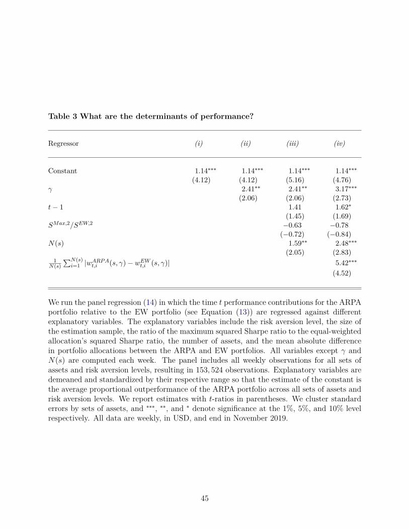
Table 3 What are the determinants of performance?

Regressor (i) (ii) (iii) (iv)

Constant 1.14∗∗∗ 1.14∗∗∗ 1.14∗∗∗ 1.14∗∗∗

(4.12) (4.12) (5.16) (4.76)γ 2.41∗∗ 2.41∗∗ 3.17∗∗∗

(2.06) (2.06) (2.73)t− 1 1.41 1.62∗

(1.45) (1.69)SMax,2/SEW,2 −0.63 −0.78

(−0.72) (−0.84)N(s) 1.59∗∗ 2.48∗∗∗

(2.05) (2.83)1

N(s)

∑N(s)i=1 |wARPA

t,i (s, γ)− wEWt,i (s, γ)| 5.42∗∗∗

(4.52)

We run the panel regression (14) in which the time t performance contributions for the ARPAportfolio relative to the EW portfolio (see Equation (13)) are regressed against differentexplanatory variables. The explanatory variables include the risk aversion level, the size ofthe estimation sample, the ratio of the maximum squared Sharpe ratio to the equal-weightedallocation’s squared Sharpe ratio, the number of assets, and the mean absolute differencein portfolio allocations between the ARPA and EW portfolios. All variables except γ andN(s) are computed each week. The panel includes all weekly observations for all sets ofassets and risk aversion levels, resulting in 153, 524 observations. Explanatory variables aredemeaned and standardized by their respective range so that the estimate of the constant isthe average proportional outperformance of the ARPA portfolio across all sets of assets andrisk aversion levels. We report estimates with t-ratios in parentheses. We cluster standarderrors by sets of assets, and ∗∗∗, ∗∗, and ∗ denote significance at the 1%, 5%, and 10% levelrespectively. All data are weekly, in USD, and end in November 2019.

45

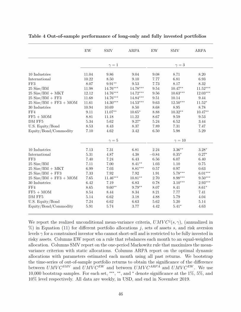
Table 4 Out-of-sample performance of long-only and fully invested portfolios

EW SMV ARPA EW SMV ARPA

γ = 1 γ = 3

10 Industries 11.04 9.86 9.04 9.08 8.71 8.20International 10.22 8.50 9.10 7.77 6.81 6.93FF3 8.07 9.91∗∗ 9.53 7.73 8.17 8.3225 Size/BM 11.98 14.76∗∗∗ 14.78∗∗∗ 9.54 10.47∗∗ 11.52∗∗∗

25 Size/BM + MKT 12.12 14.76∗∗∗ 14.72∗∗∗ 9.56 10.63∗∗∗ 12.03∗∗∗

25 Size/BM + FF3 11.68 14.76∗∗∗ 14.84∗∗∗ 9.51 10.14 9.4425 Size/BM + FF3 + MOM 11.61 14.30∗∗∗ 14.53∗∗∗ 9.63 12.50∗∗∗ 11.52∗

30 Industries 10.94 10.69 8.50 8.68 8.95 8.78FF4 9.11 11.07∗∗ 10.65∗ 8.88 10.32∗∗ 10.47∗∗

FF5 + MOM 8.81 11.18 11.22 8.67 9.59 9.53DM FF5 5.34 5.62 9.27∗ 5.24 6.52 3.44U.S. Equity/Bond 8.53 8.43 8.37 7.89 7.31 7.47Equity/Bond/Commodity 7.10 4.62 3.42 6.50 5.98 5.29

γ = 5 γ = 10

10 Industries 7.13 7.31 6.81 2.24 3.36∗∗ 3.28∗

International 5.31 4.87 4.38 −0.84 0.35∗ 0.27∗

FF3 7.40 7.24 6.43 6.56 6.07 6.4025 Size/BM 7.11 7.00 8.41∗∗ 1.03 1.10 0.7525 Size/BM + MKT 6.99 7.03 8.81∗∗∗ 0.57 0.97 0.6325 Size/BM + FF3 7.33 7.92 7.92 1.91 5.78∗∗∗ 6.01∗∗∗

25 Size/BM + FF3 + MOM 7.65 11.46∗∗∗ 10.81∗∗ 2.70 8.98∗∗∗ 9.50∗∗∗

30 Industries 6.42 7.19 6.83 0.78 3.10∗∗∗ 2.93∗∗∗

FF4 8.65 9.60∗∗ 9.79∗∗ 8.07 8.41 8.61∗

FF5 + MOM 8.54 8.44 8.34 8.21 7.77 7.41DM FF5 5.14 6.62 3.18 4.88 5.79 4.04U.S. Equity/Bond 7.24 6.62 6.63 5.62 5.20 5.14Equity/Bond/Commodity 5.91 5.74 3.77 4.42 5.41∗ 4.63

We report the realized unconditional mean-variance criteria, UMV Cj(s, γ), (annualized in%) in Equation (11) for different portfolio allocations j, sets of assets s, and risk aversionlevels γ for a constrained investor who cannot short-sell and is restricted to be fully invested inrisky assets. Columns EW report on a rule that rebalances each month to an equal-weightedallocation. Columns SMV report on the one-period Markowitz rule that maximizes the mean-variance criterion with static allocations. Columns ARPA report on the optimal dynamicallocations with parameters estimated each month using all past returns. We bootstrapthe time-series of out-of-sample portfolio returns to obtain the significance of the differencebetween UMV CSMV and UMV CEW and between UMV CARPA and UMV CEW . We use10,000 bootstrap samples. For each set, ∗∗∗, ∗∗, and ∗ denote significance at the 1%, 5%, and10% level respectively. All data are weekly, in USD, and end in November 2019.

46

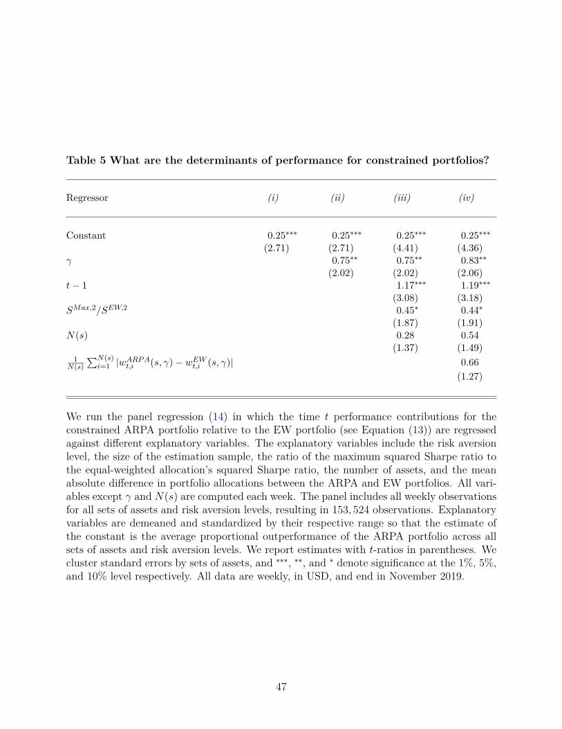
Table 5 What are the determinants of performance for constrained portfolios?

Regressor (i) (ii) (iii) (iv)

Constant 0.25∗∗∗ 0.25∗∗∗ 0.25∗∗∗ 0.25∗∗∗

(2.71) (2.71) (4.41) (4.36)γ 0.75∗∗ 0.75∗∗ 0.83∗∗

(2.02) (2.02) (2.06)t− 1 1.17∗∗∗ 1.19∗∗∗

(3.08) (3.18)SMax,2/SEW,2 0.45∗ 0.44∗

(1.87) (1.91)N(s) 0.28 0.54

(1.37) (1.49)1

N(s)

∑N(s)i=1 |wARPA

t,i (s, γ)− wEWt,i (s, γ)| 0.66

(1.27)

We run the panel regression (14) in which the time t performance contributions for theconstrained ARPA portfolio relative to the EW portfolio (see Equation (13)) are regressedagainst different explanatory variables. The explanatory variables include the risk aversionlevel, the size of the estimation sample, the ratio of the maximum squared Sharpe ratio tothe equal-weighted allocation’s squared Sharpe ratio, the number of assets, and the meanabsolute difference in portfolio allocations between the ARPA and EW portfolios. All vari-ables except γ and N(s) are computed each week. The panel includes all weekly observationsfor all sets of assets and risk aversion levels, resulting in 153, 524 observations. Explanatoryvariables are demeaned and standardized by their respective range so that the estimate ofthe constant is the average proportional outperformance of the ARPA portfolio across allsets of assets and risk aversion levels. We report estimates with t-ratios in parentheses. Wecluster standard errors by sets of assets, and ∗∗∗, ∗∗, and ∗ denote significance at the 1%, 5%,and 10% level respectively. All data are weekly, in USD, and end in November 2019.

47