a new approach to establish empirical formula for
TRANSCRIPT

International Journal of Engineering Trends and Technology Volume 69 Issue 4, 131-138, April 2021 ISSN: 2231 – 5381 /doi:10.14445/22315381/IJETT-V69I4P219 © 2021 Seventh Sense Research Group®
This is an open access article under the CC BY-NC-ND license (http://creativecommons.org/licenses/by-nc-nd/4.0/)
A New Approach to Establish Empirical Formula
for Estimating Fishing Boat Resistance
Chinh Van Huynh1, Ha Vu Nguyen2, Thai Gia Tran3
1Ph.D. Student, Department of Shipbuilding Technology, Ho Chi Minh City University of Transport, Viet Nam 2Ph.D. Student, Fishing Vessel Registration Center - Directorate of Fisheries, Viet Nam
3 Associate Professor, Department of Naval Architecture and Marine Engineering, Nha Trang University, Viet Nam
Abstract – Resistance estimation is the basis for solving
many important problems in ship design, such as selecting
the suitable propulsion system, optimizing the hull form, etc.
Three methods commonly used to estimate ship resistance
are an empirical method, CFD analysis, and model testing.
Compared with the last two ones, the empirical method in
the form of approximate curves or formulas allow estimating
resistance very fast without effort, cost, or ship lines, etc.
However, it is extremely difficult and costly to establish such
curves or formulas, and they also rarely give the expected accuracy when computational ships differ from test ships. In
this paper, we present a simple approach to obtain an
empirical formula for accurately estimating the resistance of
fishing boats based on the existing model test data of the
Food and Agriculture Organization (FAO) of the United
Nations. The application of the research results to the
Vietnamese fishing fleet has validated the reliability of this
approach when the deviations of the resistance values
calculated from the established empirical formula and the
corresponding model and actual test data are within 4%.
Keywords — empirical formula, FAO, fishing boat,
resistance, Vietnamese.
I. INTRODUCTION
Resistance estimation is one of the first problems that
need to be solved in the ship design process and is the main
basis for solving many other important problems such as
selecting the right propulsion system, optimizing the hull
form, etc. Therefore, there have been many studies trying to
find out how to determine the ship resistance quickly and
accurately. Until now, the three methods commonly used to
estimate ship resistance are computational fluid dynamics method or also know as CFD analysis, model testing, and
empirical method. CFD analysis is a modern method that has
been widely used recently, which involves creating a
complete 3D hull model and performing a numerical
simulation of fluid flow around it to compute the
hydrodynamic forces acting on the hull [1]. However, CFD
analysis takes a lot of time, effort and does not always
provide highly accurate resistance results [2]. Also, it can be
costly and requires the ship's lines drawing.
Model testing is the most accurate and reliable method for
estimating resistance based on building a scaled-down
model of the real ship, testing to determine the model
resistance in a towing tank, and transfer the model resistance
to a real ship [3]. However, model tests are quite cost-
prohibited, so it is often performed in necessary cases or to
validate the other methods. The empirical method is
presented in the form of the approximate curves or formulas/
equations, which are established based on systematizing
model test data set of a series of ships with similarities in geometrical characteristics and hull form [3]. Due to such an
approach, there are many empirical curves or formulas that
are applied to different types of ships, and the result of the
empirical curves or formulas are also different. Some well-
known empirical resistance formulas can be listed, such as
Holtrop-Mennen's formula for conventional ships [4], the
formula for the planing hull of Savisky [5], Blount [6], or
Doust’s regression equation for fishing boats [7], etc.
Compared with the above two methods, the empirical
method allows estimating the resistance very quickly with
limited initial data without effort, cost, or availability of ship
lines. But the establishment of empirical formulas is extremely difficult and expensive, and their accuracy is
often uncertain due to the differences between calculated
ships and those which were used in the model test to
establish the formulas.
Starting in 1950 and for a long time, a model test dataset
of 576 fishing boats was performed or sponsored by the
Food and Agriculture Organization of the United Nations
(FAO). Then, FAO scientists Hayes (1964) and Doust
(1969) had made a regression analysis of this dataset to
establish the empirical formula for estimating the resistance
of trawlers [8]. It is worth mentioning that FAO model test data was collected for a very large number of fishing boats
in many countries, with the hull form parameters varying in
a fairly wide range. So the empirical formula established
based on this data may not ensure the desired accuracy when
applied to specified fishing boat fleets whose hull
parameters vary within small ranges, or outside the defined
range of valid hull parameters. In this paper, we present a
simple approach to establishing an empirical formula to
accurately estimate the resistance of a specific type of
fishing boat based on FAO model test data.

Thai Gia Tran et al. / IJETT, 69(4), 131-138, 2021
132
II. MATERIAL AND RESEARCH METHOD
In term of the method, the empirical resistance formula
will be established based on fishing boat model test data,
which was published in two FAO publications: Computer-
aided studies of fishing boat hull resistance (Hayes and Engvall, 1969) [9] and Fishing Boat Tank Test (Jan-Olof
Traung, 1965) [10]. The first document presents the model
test data tables of 576 fishing boats collected from all FAO
member states, while the second one presents the hull lines
and resistance curves of 250 fishing boats that have been
tested in the European tanks. Base on these two documents,
an empirical formula for estimating the resistance of a
specific type of fishing boats, called research fishing boats,
can be established according to the following steps:
(1) Analysis of the hull lines of research fishing boats to
determine variation ranges of the hull form parameters
which have a great effect on the resistance of common
ships in general, fishing boats in particular.
(2) Analysis of the hull lines in document [9] to select the
fishing boat models with hull lines and hull form
parameters similar to the research fishing boats.
(3) Establish a model test data set to formulate the empirical
formula for estimating the resistance of the research
fishing boats as follows:
(i) Analysis of the model test data tables in document
[10] to select the model test data set corresponding to
the variation range of the hull form parameters of the
research fishing boats determined in step (1).
(ii) Digitize the resistance curves of the fishing boats
selected in step (2) to determine the resistance test
data and add them to the resistance test data set
already in step (i) to obtain a new resistance test data
set suitable for research fishing boats.
(4) Perform a regression for test data set already in step (ii)
to establish the empirical resistance formula for the
research fishing boats.
(5) Compare the resistance values calculated from the
established formula and from the model and actual test
of some research fishing boats to evaluate the accuracy
and reliability of this approach in general and the
empirical formula in particular.
III. RESULTS AND DISCUSSIONS
The following section presents the results and discussions
of applying this approach to establish the empirical formula
for estimating the resistance of the Vietnamese fishing fleet.
A. Analysis of the Hull Lines of Vietnamese Fishing Boats
The total number of fishing boats in Vietnam today is
more than 120,000, but most are wooden and composite hull
boats. Steel fishing vessels account for a low proportion,
below 2%. One of our research projects carried out in 2014
with funding from the Vietnamese Government has
identified the basic features of the Vietnamese fishing fleet
as follows [11].
a) Features of hull form parameters:
Our studies have shown that the variation range of the hull
form parameters of Vietnamese fishing fleets depends on
many factors such as fishing ground, type of fishing gear, etc. Table 1 shows the variation range of hull form
parameters of Vietnamese fishing boats of FAO model test
dataset, and the study range was selected based on these two
ranges [11].
Table 1. The variation range of hull form parameters
Parameters FAO
data
Vietnamese
fishing boats
Study range
VS/ gL 0.35 0.20 ÷ 0.40 0.20 ÷ 0.40
L/B 3.10 ÷ 5.60 3.20 ÷ 5.00 3.20 ÷ 5.00
B/T 2.00 ÷ 4.50 2.20 ÷ 4.20 2.20 ÷ 4.20
L/1/3 3.75 ÷ 5.00 3.50 ÷ 5.50 3.75 ÷ 5.00
CB 0.55 ÷ 0.72 0.55 ÷ 0.72
CP 0.55 ÷ 0.70 0.65 ÷ 0.73 0.65 ÷ 0.70
CM 0.53 ÷ 0.93 0.85 ÷ 0.92 0.85 ÷ 0.92
LCB = Xc/L (%) - 4.0 ÷ 2.0 -3.7 ÷ 0.0 -3.7 ÷ 0.0
1/2 αE (dgree) 15 ÷ 35 20 ÷ 42 20 ÷ 35
1/2 αR (dgree) 30 ÷ 80 - 30 ÷ 60
TRIM -0.04 ÷ 0.08 - -0.04 ÷ 0.08
A/Amax 0.00 ÷ 0.02 0.00 ÷ 0.02
Nomenclature in Table 1.
VS/ gL - the ratio of the shipping speed to the
length.
L/1/3 - the ratio of the length to the displacement.
CB, CP, CM - block, prismatic, and mid-ship coefficients.
1/2 αE, 1/2αR - half-angle of entrance and exit,
respectively.
LCB - longitudinal centre of buoyancy.
L/B, B/T - ratio of the length to the breadth, and ratio
of the breadth to the draft, respectively.
A/Amax - ratio of the keel cross-sectional area to the maximum transverse section area.
TRIM - the difference between the drafts forwards
and aft.
b) Features of hull lines:
The hull lines of Vietnamese fishing boats are quite
similar to some of the fishing boats which were used in
model testing by FAO, with two basic types: round bottom hull as shown in Fig. 1a, and chine hull as shown in Fig.1b.

Thai Gia Tran et al. / IJETT, 69(4), 131-138, 2021
133
(a) round-bottom (b) chine hull
Fig. 1. Hull lines of Vietnamese steel fishing boats
B. Establish the resistance test data suitable for
Vietnamese fishing boats.
a) Determining resistance test data from FAO data:
The FAO model testing data in document [9] are presented
in tabular form depending on the known hull form
parameters. On these tables, the model test data corresponding to the variation range of hull form parameters
of Vietnamese fishing boats will be marked (shaded
rectangles) as shown in Table 2. Many such tables are
processed to select all matching data.
Table 2. Marking selected areas on FAO data tables L/B=3.7 B/T=2.8 Cp VS/ L = 1.1
L/Δ1/3 ½αE CM at
CP=0.55 0.575 0.600 0.625 0.650 0.675
CM at
CP=0.70
3.75
15.0 1.32 1.04
17.5
20.0
25.0
30.0
35.0
4.00
15.0 1.09 20.48 18.77 17.66 16.80 15.95 0.86
17.5 20.90 19.34 18.37 17.65 16.94
20.0 21.57 20.15 19.32 18.74 18.18
25.0 23.05 21.91 21.37 21.08 21.81
30.0 23.96 23.11 22.85 22.84 22.86
35.0 23.60 23.04 23.07 23.35 23.64
4.25
15.0 0.91 17.31 16.02 15.61 15.67 15.87 15.99 15.87 0.71
17.5 17.45 16.30 16.03 16.23 16.58 16.85 16.86
20.0 17.82 16.82 16.70 17.04 17.53 17.94 18.10
25.0 18.73 18.02 18.18 18.81 19.58 20.28 20.72
30.0 19.07 18.64 19.08 20.00 21.06 22.04 22.77
35.0 18.14 18.00 18.73 19.93 21.28 22.55 23.56
4.50
15.0 0.77 15.91 15.61 15.88 16.38 16.86 17.12 17.04 0.60
17.5 16.05 15.89 16.30 16.94 17.56 17.97 18.03
20.0 16.43 16.42 16.97 17.75 18.51 19.06 19.27
25.0 17.34 17.61 18.45 19.52 20.57 21.40 21.90
30.0 17.67 18.23 19.35 20.71 22.05 23.17 23.95
35.0 16.74 17.59 19.00 20.64 22.26 23.67 24.74
4.75
15.0 0.65 16.85 16.70 16.99 17.44 17.81 17.93 17.68 0.51
17.5 16.99 16.98 17.42 18.01 18.52 18.78 18.68
20.0 17.37 17.50 18.08 18.81 19.47 19.88 19.92
25.0 18.28 18.70 19.56 20.58 21.52 22.22 22.54
30.0 18.61 19.32 20.47 21.77 23.00 23.98 24.59
35.0 17.68 18.68 20.11 21.71 23.22 24.48 25.38
5.00
15.0 0.56 17.79 17.48 17.59 17.83 17.99 17.90 17.45 0.44
17.5 17.93 17.76 18.01 18.40 18.70 18.75 18.44
20.0 18.30 18.28 18.68 19.20 19.65 19.85 19.68
25.0 1.32 19.21 19.48 20.16 20.97 21.70 22.19 22.31
30.0 19.55 20.10 21.06 22.16 23.18 23.95 24.35
35.0 18.62 19.46 20.71 22.10 23.40 24.45 25.14
Selection of resistance correction coefficients CR due to
the effect of other hull form parameters is shown in the
following tables, from Table 3 to Table 5.
Table 3. Correction CR1 due to effect of 1/2R and CP
½αR
(degree)
CP
0.550 0.575 0.600 0.625 0.650 0.675 0.700
20 -0.53 -0.41 -0.29 -0.18 -0.06 0.06 0.17
25 0.00 0.00 0.00 0.00 0.00 0.00 0.00
30 0.44 0.32 0.21 0.09 -0.03 -0.14 -0.26
35 0.80 0.56 0.33 0.09 -0.14 -0.37 -0.61
40 1.06 0.71 0.36 0.01 -0.37 -0.69 -1.04
Table 4. Correction CR2 due to effect of 1/2R and LCB
LCB
(%)
½αE (degree)
15 17.5 20 25 30 35
2.0 1.43 0.62 0.00 -0.69 -0.65 0.13
0.0 0.66 0.28 0.00 -0.29 -0.21 0.24
-2.0 0.00 0.00 0.00 0.00 0.00 0.00
-4.0 -0.54 -0.22 0.00 0.17 -0.02 -0.58
Table 5. Correction CR3 due to effect of TRIM TRIM -0.04 -0.01 0.02 0.05 0.08 0.11
CR3 -0.49 -0.33 -0.16 0.00 0.16 0.33
Table. 6. Correction CR4 due to effect of A/Amax A/Amax 0 0.01 0.02 0.03 0.04 0.05
CR4 0 2.25 4.34 6.43 8.52 10.61
To conform to the regression analysis, the selected data are
rearranged in a new table as the resistance coefficient CR16
(resistance coefficient of the 16-ft model is used to calculate
FAO model test data) as a function of hull form parameters.
The first part of this new resistance data table is shown in
Table 7, and of course, a table with such data is very large.
Table 7. The resistance data for regression analysis in the
form CR16 = f(L/B, B/T, CM, CP, ½αE)
Resistance
coefficient CR16
Hull form parameters
L/B B/T CM CP ½ αE
16.73 3.1 2.6 0.861 0.550 20
16.88 3.1 2.6 0.861 0.550 25
16.47 3.1 2.6 0.861 0.550 30
14.61 3.1 2.6 0.861 0.550 35
19.98 3.1 2.8 0.928 0.550 20
19.07 3.1 2.8 0.888 0.575 20
18.85 3.1 2.8 0.851 0.600 20
19.94 3.1 2.8 0.928 0.550 25
19.31 3.1 2.8 0.888 0.575 25
19.38 3.1 2.8 0.851 0.600 25
19.46 3.1 2.8 0.928 0.550 30
19.13 3.1 2.8 0.888 0.575 30
19.48 3.1 2.8 0.851 0.600 30
17.65 3.1 2.8 0.928 0.550 35
17.60 3.1 2.8 0.888 0.575 35
18.24 3.1 2.8 0.851 0.600 35
21.72 3.1 3.0 0.911 0.600 20
21.09 3.1 3.0 0.875 0.625 20
22.11 3.1 3.0 0.911 0.600 25
21.77 3.1 3.0 0.875 0.625 25
22.19 3.1 3.0 0.911 0.600 30
22.14 3.1 3.0 0.875 0.625 30
21.04 3.1 3.0 0.911 0.600 35
21.27 3.1 3.0 0.875 0.625 35
22.86 3.1 3.2 0.897 0.650 20
21.33 3.1 3.2 0.864 0.675 20
23.74 3.1 3.2 0.897 0.650 25
22.50 3.1 3.2 0.864 0.675 25
24.41 3.1 3.2 0.897 0.650 30
23.46 3.1 3.2 0.864 0.675 30
23.98 3.1 3.2 0.897 0.650 35
In addition, it should be noted that these resistance data
were calculated based on resistance coefficient (CR16) in the
American measurement system, so it is necessary to perform

Thai Gia Tran et al. / IJETT, 69(4), 131-138, 2021
134
a conversion to the total ship resistance (R) in the metric
system by the following formula:
R = CRL
V2s
(1)
where is displacement (T-Longton), VS is ship speed (knot), L is ship length (feet), CR is total resistance
coefficient calculated by the following formula:
CR = CR16 + CR1 + CR2 + CR3 + CR4 (2)
with resistance coefficient CR16 is calculated from Table 7,
CR1, CR2, CR3, CR4 are respectively corrections due to
effect of hull form parameters such as 1/2R and CP (Table
3), 1/2R and CP (Table 4), TRIM (Table 5), A/Amax (Table
6). The full data tables above can be found in the reference
[12].
b) Determine resistance test data from specific boats:
Model test data in the form of effective power curves of a
large number of fishing boats are presented in the document
[10]. A comparative study was performed to select the FAO-
tested fishing boats with features of the hull lines and
variation range of hull form parameters similar to
Vietnamese fishing boats. As a result, sixteen fishing boats
were selected with their hull form parameters, and model test
cases are shown in Table 8.
Table 8. Hull form parameters of selected fishing boats
Ship Case Hull Form Parameters
L B LCB CP CB L/B B/T 1/2aE L/1/3
FA076
I 39.50 9.76 -1.1 0.596 0.524 4.04 2.56 19.5 4.26
II 39.80 9.76 -2.5 0.597 0.525 4.08 2.56 19.0 4.29
III 40.10 9.76 -6.7 0.656 0.577 4.11 2.286 18.0 4.01
FA075
I 44.20 10.36 -1.1 0.581 0.524 4.26 2.266 18.5 4.18
II 44.45 10.36 -1.6 0.586 0.53 4.28 2.266 16.7 4.29
III 44.55 10.36 -3.0 0.597 0.542 4.3 2.192 17.0 4.22
FA074
I 44.20 10.36 -1.1 0.584 0.527 4.26 2.266 18.5 4.26
II 44.45 10.36 -1.9 0.590 0.534 4.28 2.266 16.7 4.28
III 44.55 10.36 -3.2 0.606 0.55 4.30 2.192 17.0 4.20
FAO73
I 44.20 10.36 -0.9 0.583 0.526 4.26 2.266 13.0 4.28
II 44.45 10.36 -1.5 0.591 0.535 4.28 2.266 11.0 4.28
III 44.55 10.36 -3.0 0.607 0.551 4.3 2.192 9.0 4.20
FAO72
I 44.20 10.36 -0.7 0.58 0.523 4.26 2.266 13.0 4.28
II 44.45 10.36 -1.3 0.586 0.53 4.28 2.266 11.0 4.29
III 44.55 10.36 -2.5 0.598 0.543 4.30 2.192 9.0 4.26
FAO71 39.60 6.712 -0.9 0.66 0.504 5.81 2.28 23.0 5.33
FAO70 39.00 7.884 -0.9 0.66 0.504 4.95 2.28 25.0 4.79
FAO69 39.80 7.3 -0.9 0.66 0.504 5.34 2.28 23.5 5.04
FAO68 39.30 7.0 -1.3 0.666 0.522 5.62 1.94 22.5 4.91
FAO64 42.00 7.6 -0.6 0.673 0.526 5.53 2.305 23.5 5.10
FAO63 38.80 7.3 -0.4 0.652 0.487 5.33 2.415 21.0 5.16
FAO61 I 38.00 7.0 -0.7 0.648 0.496 5.43 2.29 25.0 5.13
II 38.00 7.0 -6.0 0.658 0.458 5.43 2.665 17.5 5.54
FAO18 39.65 8.7 0.1 0.570 0.460 4.56 2.38 16.0 4.53
FAO15 47.30 10.6 -0.8 0.667 0.556 4.47 2.71 20.5 4.66
FAO13 42.70 10.0 -0.6 0.615 0.538 4.25 2.442 24.5 4.34
FAO12 41.20 10.3 -0.8 0.607 0.459 3.99 2.733 26.5 4.56
Next, the effective power curves of the selected fishing
boats are digitized to determine the second resistance test
data which is also arranged in a similar table as shown in
Table 7. A portion of the data table is shown in Table 9, and
similar to the above tables, this full data table is also very
large.
Table 9. The effective power test data L(m) B(m) LCB(m) CP CB L/B B/T 1/2aE L/V1/3 Fn EHP(HP)
44.20 10.36 -0.70 0.58 0.523 4.26 2.266 13 4.18 0.325 687.85
44.45 10.36 -1.30 0.586 0.53 4.28 2.266 11 4.29 0.325 703.51
44.55 10.36 -2.50 0.598 0.543 4.30 2.192 9 4.22 0.325 734.77
44.20 10.36 -0.90 0.583 0.526 4.26 2.266 13 4.26 0.325 750.38
44.45 10.36 -1.50 0.591 0.535 4.28 2.266 11 4.28 0.325 781.65
44.55 10.36 -3.00 0.607 0.551 4.30 2.192 9 4.20 0.325 844.18
44.20 10.36 -1.10 0.584 0.527 4.26 2.266 18.5 4.28 0.325 859.81
44.45 10.36 -1.95 0.59 0.534 4.28 2.266 16.7 4.28 0.325 862.94
44.55 10.36 -3.20 0.606 0.55 4.30 2.192 17 4.20 0.325 969.24
44.20 10.36 -1.10 0.581 0.524 4.26 2.266 18.5 4.28 0.325 687.85
44.45 10.36 -1.60 0.586 0.53 4.28 2.266 16.7 4.29 0.325 719.12
44.55 10.36 -3.00 0.597 0.542 4.30 2.192 17 4.26 0.325 750.38
44.20 10.36 -0.70 0.58 0.523 4.26 2.266 13 4.18 0.35 1000.51
44.45 10.36 -1.30 0.586 0.53 4.28 2.266 11 4.29 0.35 1031.78
44.55 10.36 -2.50 0.598 0.543 4.30 2.192 9 4.22 0.35 1094.31
44.20 10.36 -0.90 0.583 0.526 4.26 2.266 13 4.26 0.35 1100.56
44.45 10.36 -1.50 0.591 0.535 4.28 2.266 11 4.28 0.35 1106.56
44.55 10.36 -3.00 0.607 0.551 4.30 2.192 9 4.20 0.35 1188.11
44.20 10.36 -1.10 0.584 0.527 4.26 2.266 18.5 4.28 0.35 1188.11
44.45 10.36 -1.95 0.59 0.534 4.28 2.266 16.7 4.28 0.35 1203.74
Convert effective power into resistance and combine two
defined data sets into a set to establish the empirical formula
for estimating the resistance of Vietnamese fishing boats.
C. Establish Resistance Regression Formular
The process of establishing a regression formula based on
identified resistance test data was performed using SPSS [13], a common statistical analysis software today, in two
steps:
Perform a correlation analysis to determine and include
regression equation for the hull form parameters that
have a great effect on resistance.
Perform a regression analysis to find a resistance
formula as a function of the selected hull form
parameters.
a) Correlation analysis of hull form parameters:
Table 9 presents the results of correlation analysis of hull
form parameters to resistance values based on the resistance
data set, which was determined in section B.
Table 9. Correlation analysis of hull form parameters
with resistance R L B LCB CM CB CP ½αE R
L
Pearson
Correlation
Sig(2-tailed)
1
.824
.000
.058
.385
-.433
.000
.653
.000
.755
.000
-.521
.000
.889
.000
.373
.000
B
Pearson
Correlation
Sig(2-tailed)
.824
.000
1
-.041
.540
-.691
.000
.533
.000
.833
.000
-.496
.000
.934
.000
.344
.000
LCB
Pearson
Correlation
Sig(2-tailed)
.058
.385
-.041
.540
1
-.165
.013
-.279
.000
-.089
.183
-.271
.000
-.111
.097
-.070
.295
CP Pearson
Correlation
Sig(2-tailed)
-.433
.000
-.691
.000
-.165
.013
1
-.049
.466
-.706
.000
.562
.000
-.664
.000
-.325
.146
CB Pearson
Correlation
Sig(2-tailed)
.653
.000
.533
.000
.279
.000
-.049
.466
1
.741
.000
-.386
.000
.699
.000
.254
.132
CM Pearson
Correlation
Sig(2-tailed)
.755
.000
.833
.000
-.089
.183
-.706
.000
.741
.000
1
-.659
.000
.939
.000
.403
.000
½αE Pearson
Correlation
Sig(2-tailed)
-.521
.000
-.496
.000
.271
.000
.562
.000
-.386
.000
-.659
.000
1
-.653
.000
.348
.000
Pearson .889 .934 -.111 -.664 .699 .939 -.653 1 .415

Thai Gia Tran et al. / IJETT, 69(4), 131-138, 2021
135
Correlation
Sig(2-tailed)
.000
.000
.097
.000
.000
.000
.000
.000
R Pearson
Correlation
Sig(2-tailed)
.373
.000
.344
.000
-.070
.295
-.325
.146
.254
.132
.403
.000
-.348
.000
.415
.000
1
The meaning and determination of the Pearson correlation
coefficient (r) and the significant value of the Pearson test
(Sig.) in Table 9 can be found in the statistical literature [14].
The results in this table show the parameters L, B, CP, 1/2E,
are strongly correlated with resistance because the value
of Sig (2-tailed) is less than .05 and the Pearson coefficient
is high. The similar correlations of remaining parameters
LCB, CM, CB with resistance are not or very weak because the value of Sig (2-tailed) is greater than .05 and the Pearson
coefficient is small, so they can be ignored in the resistance
regression equation. This is also consistent with the fact
because the effects of the ignored parameters on resistance
are taken into through their relationships with the parameters
in the regression equation. Different from FAO’s previous
resistance empirical formulas, a speed parameter is included
in the regression equation so that resistance values can be
calculated at different boat speeds. Based on these analyses,
resistance regression equation can be established as a
function as follows:
R = f(L, B, CP, 1/2E, , VS) (3)
b) Regression analysis of resistance data:
Table 10 shows the results of regression analysis for the
defined resistance test data set using SPSS.
Table 10. The results of regression analysis for the
defined resistance test data set
Types of
regression
functions
Regression parameters
R R2 Ra2 Std.
Error R R2 Ra2
Std.
Error
L - R CM - R
LINEAR .627 .393 .391 456.610 .633 .401 .398 453.846
LOGARITHMIC .615 .379 .376 462.065 .407 .166 .162 535.351
INVERSE .591 .350 .347 472.774 .583 .340 .337 476.081
QUADRATIC .676 .457 .452 432.903 .692 .479 .475 423.943
CUBIC .675 .455 .450 433.657 .695 .483 .478 422.463
COMPOUND .977 .954 .954 1.140 .978 .957 .957 1.097
POWER .974 .948 .948 1.208 .819 .670 .669 3.051
S CURVES .964 .929 .929 1.414 .960 .921 .920 1.495
GROWTH .977 .954 .954 1.140 .978 .957 .957 1.097
EXPONENTIAL .977 .954 .954 1.140 .978 .957 .957 1.097
LOGISTICS .977 .954 .954 1.140 .978 .957 .957 1.097
B – R D – R
LINEAR .642 .412 .409 449.649 .680 .462 .460 429.779
LOGARITHMIC .627 .393 .390 456.641 .627 .393 .390 456.637
INVERSE .560 .314 .311 485.553 .435 .189 .185 527.913
QUADRATIC .671 .451 .446 435.449 .701 .492 .487 418.794
CUBIC .673 .453 .448 434.456 .708 .501 .494 416.092
COMPOUND .977 .954 .954 1.139 .965 .931 .930 1.400
POWER .977 .954 .953 1.144 .977 .955 .954 1.132
S CURVES .944 .891 .891 1.752 .837 .701 .700 2.906
GROWTH .977 .954 .954 1.139 .965 .931 .930 1.400
EXPONENTIAL .977 .954 .954 1.139 .965 .931 .930 1.400
LOGISTICS .977 .954 .954 1.139 .965 .931 .930 1.400
1/2aE - R V - R
LINEAR .513 .263 .259 503.333 .763 .582 .580 379.077
LOGARITHMIC .578 .334 .331 478.258 .682 .465 .462 428.899
INVERSE .658 .432 .430 441.656 .435 .189 .186 527.811
QUADRATIC .663 .440 .435 439.763 .918 .842 .841 233.316
CUBIC .673 .453 .446 435.403 .938 .880 .878 203.982
COMPOUND .908 .824 .823 2.228 .993 .986 .986 .635
POWER .956 .914 .913 1.561 .991 .983 .982 .703
S CURVES .950 .902 .902 1.660 .876 .767 .766 2.564
GROWTH .908 .824 .823 2.228 .993 .986 .986 .635
EXPONENTIAL .908 .824 .823 2.228 .993 .986 .986 .635
LOGISTICS .908 .824 .823 2.228 .993 .986 .986 .635
The meaning and determination of the quantities included
in Table 10, such as multiple regression (R), R square (R2),
adjusted R square ( 2aR ), and standard error of the estimate
(Std. Error), can be found in the literature on statistics [14].
The result in Table 10 shows among 11 types of regression
functions in SPSS, and the power function is the most suitable because the value of the R coefficient is the
correlation between the actual and predicted value of all
independent variables on the resistance data of this function
is the highest. Thus, a power function correlation between
resistance and hull form parameters can be assumed for the
resistance formula. Also, the R-square values when
estimating regression for the power function of all
independent variables are high, so it can be assumed the
relationship between the dependent variable (resistance) and
each independent variable in this function (hull form
parameter) is also in the form of power functions. However,
the results of the above analysis are not final due to at this time, only the correlation between the dependent variable
and each dependent variable has been determined, while the
correlation between these variables is complicated due to the
interactions between independent variables.
Therefore, the general form of the resistance regression
equation can be determined as follows:
R =
k
0i
nS
nnP
n
Enn
i6i5i4i
3i
2i1i VC2
1BLa (4)
where ai is the coefficient of the regression equation.
After many regression calculations, it can be seen that
with k = 3, the resistance values calculated from the
regression equation is very close to actual values, therefore,
can be expressed the resistance regression equation as
follows:
RT = 11109765432 aE
aa8
aS
aaP
aE
aa1 5.0BLaV.C.5.0.B.La
212019181716141312 aS
aaP
aE
aa15
aaaP V.C.5.0.B.LaV.C (5)
where the values of the coefficients (ai) are determined using
SPSS and shown in Table 11.
Table 11. The coefficients (ai) of the regression equation
Coefficients Estimate Std. Error 95% Confidence Interval
Lower Bound Upper Bound
a1 4.22612E-12 2.6949E-11 -4.89081E-11 5.73603E-11
a2 1.695053715 1.455895235 -1.17547798 4.56558541
a3 -8.364176195 2.19208219 -12.68621891 -4.042133475
a4 0.632238254 0.382341928 -0.121610372 1.386086879
a5 -14.83655878 5.305919959 -25.29803365 -4.375083917
a6 4.124515702 1.622580352 0.925337481 7.323693922
a7 4.429483057 0.404931712 3.631095037 5.227871077
a8 1.09309E-15 1.45796E-12 -2.87351E-12 2.87569E-12
a9 -65.08529955 28.57271831 -121.4210107 -8.749588364
a10 108.4864185 574.2726774 -1023.784559 1240.757396
a11 0.000318457 0.142673202 -0.280984715 0.28162163
a12 111.1408698 39.2923986 33.66958426 188.6121554
a13 -1.962374239 1.55261026 -5.023595165 1.098846686
a14 21.72051439 3.178536419 15.45351845 27.98751033
Thai Gia Tran et al. / IJETT, 69(4), 131-138, 2021
136
a15 40491.08902 322373.0298 -595119.2057 676101.3837
a16 -19.72536623 4.880552085 -29.3481599 -10.10257257
a17 28.38449642 7.088653736 14.40807509 42.36091775
a18 0.04766876 0.06970403 -0.089763949 0.185101469
a19 31.21465383 6.770105818 17.86630098 44.56300669
a20 -0.140557962 0.513933176 -1.153859906 0.872743981
a21 3.242442101 0.153314285 2.940158322 3.544725879
The meaning and determination of the quantities in Table
10 can be found in the literature on SPSS [13] or statistics
[14].
D. Validate established resistance formula
The accuracy and reliability of the established empirical
formula are evaluated and validated by comparing resistance
calculated from the empirical formula (empirical resistance)
and the model test data (test resistance) of some Vietnam
fishing boats, including steel and wooden hull.
a) For the wooden fishing fleet:
Vietnamese wooden fishing boats are built according to
long-time traditional patterns with their overall length of
fewer than 25 meters, straight bow, transom stern, a large
keel on the bottom extending from stern to bow to create the
hull strength. The hull form depends on the fishing ground,
fishing gear, local model, etc. but not much different with the
cross-sections having U-shaped and gradual changing to V-
shape in the bow region to develop the exploitation deck in
the forebody [11]. Until now, four typical Vietnamese
wooden fishing boats, denoted M1317A, M1319, M250-2,
MH076, have been tested in towing tanks to determine resistance data [15], [16], [17].
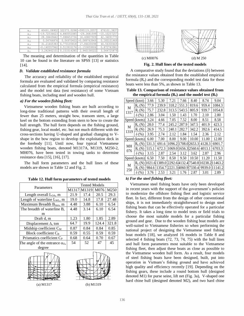
The hull form parameters and the hull lines of these models are shown in Table 12 and Fig. 2.
Table 12. Hull form parameters of tested models
Parameters Tested Models
M1317 M1319 M076 M250
Length overall LOA, m 21.9 17.4 20.5 29.3
Length of waterline LWL, m 19.0 14.8 17.8 27.48
Maximum Breadth Bmax, m 4.48 3.88 6.10 6.54
The breadth of waterline B,
m
4.48 3.14 6.10 6.54
Draft d, m 1.23 1.80 1.85 2.89
Displacement , ton 64.7 19.9 124.4 321.8
Midship coefficient CM 0.87 0.84 0.84 0.85
Block coefficient CB 0.59 0.55 0.59 0.59
Prismatics coefficient CP 0.68 0.64 0.70 0.67
The angle of the entrance E,
degree
54 52 47 45
(a) M1317 (b) M1319
(c) MH076 (d) M 250
Fig. 2. Hull lines of the tested models
A comparative study found that the deviations () between
the resistance values obtained from the established empirical
formula (Re) and the corresponding model test data for these
boats were less than 5%, as shown in Table 13.
Table 13. Comparison of resistance values obtained from
the empirical formula (Re) and the model test (Rt)
Speed (knot) 3.66 5.30 7.21 7.66 8.40 8.74 9.04
M
1317
Re (N) 77.9 239.9 318.2 551.3 819.6 959.4 1084.3
Rt (N) 75.7 232.8 313.5 543.5 805.9 939.7 1054.8
(%) 2.86 3.04 1.50 1.43 1.70 2.10 2.80
Speed (knots) 3.24 4.66 7.05 7.52 8.00 8.51 8.58
M
1319
Re (N) 28.0 77.4 245.2 287.9 347.5 401.9 423.3
Rt (N) 26.9 75.3 240.1 282.7 342.2 392.6 414.5
(%) 3.95 2.74 2.12 1.84 1.54 2.36 2.12
Speed (knots) 6.00 7.00 8.00 9.00 10.00 11.00 12.00
MH
076
Re (N) 531.3 691.6 1096.2 1708.0 2653.3 4128.3 6901.7
Rt (N) 515.1 672.3 1069.0 1656.3 2560.6 4013.1 6703.3
(%) 3.15 2.87 2.54 3.12 3.62 2.87 2.96
Speed (knots) 6.50 7.50 8.50 9.50 10.50 11.20 11.50
M
250
Re (N) 1021.6 1389.0 2292.6 4132.4 7540.8 10238.2 11463.2
Rt (N) 984.6 1354.7 2221.3 4060.9 7330.4 9939.0 11141.2
(%) 3.76 2.53 3.21 1.76 2.87 3.01 2.89
b) For the steel fishing fleet:
Vietnamese steel fishing boats have only been developed
in recent years with the support of the government’s policies
to modernize the offshore fishing fleet and logistic service
fleet. In fact, different from the design of other conventional ships, it is not immediately straightforward to design steel
fishing boats that can be effectively operated for a particular
fishery. It takes a long time to model tests or field trials to
choose the most suitable models for a particular fishing
ground and gear. Due to the wooden fishing boat models are
well-suited to Vietnamese fisheries so when performing the
national project of designing the Vietnamese steel fishing
boat models [18], we analyzed 16 models in Table 8 and
selected 4 fishing boats (72, 73, 74, 75) with the hull lines
and hull form parameters most suitable to the Vietnamese
fishing fleet, then adjust these boats as close as possible to the Vietnamese wooden hull form. As a result, four models
of steel fishing boats have been designed, built, put into
operation in Vietnam’s fishing ground and have achieved
high quality and efficiency recently [19]. Depending on the
fishing gears, these include a round bottom hull (designed
denoted M1) for purse seine, lift net (Fig. 3a), V-shaped one
hard chine hull (designed denoted M2), and two hard chine

Thai Gia Tran et al. / IJETT, 69(4), 131-138, 2021
137
hull (designed denoted M3) for gill net, trawler (Fig. 3b, 3c),
or U-shaped chine hull (designed denoted M4) for hook and
line (Fig. 3d).
(a) M1 - Round bottom hull
(b) M2 - U-shaped soft chine hull
(c) V-shaped hard one chine hull
(c) V-shaped hard two chine hull
Fig. 3. Four hull lines of Vietnamese steel fishing boat
models
The hull form parameters of the four above steel fishing
boat models are shown in Table 14.
Table 14. Hull parameters of steel fishing boat models
Parameters Models
M1 M2 M3 M4
Length overall LOA, m 29.0 32.5 27.0 30.8
Length of waterline LWL, m 26.5 30.5 24.8 27.2
The breadth of waterline B, m 6.35 7.32 5.70 6.45
Draft d, m 2.75 3.05 2.20 2.70
Displacement , ton 247.8 393.2 173.1 268.6
Midship coefficient Cm 0.84 0.92 0.85 0.90
Angle of entrance E (degree) 40 45 40 45
Horsepower (HP) 900 1200 830 1000
Speed (knots) 10.5 11.5 10.0 10.5
A comparison study between the required horsepower
values obtained from the empirical formula (Ne) and the
actual test (Nt) [20] for these fishing boats under no-load
(case I) and full-load (case II) showed a well-suited with
actual operation as shown in Table 15. S
Table 15. Comparison of resistance values obtained from
the empirical formula (Re) and the model test (Rt)
Speed (knots) 7 8 9 10 11 12
M1
I
Ne (HP) 376.0 494.6 558.0 671.8 911.5 1327.7
Nt (HP) 389.9 480.0 551.7 660.9 883.2 1281.3
(%) -3.56 3.03 1.14 1.65 3.21 3.62
II
Ne (HP) 390.1 506.3 564.0 703.4 939.5 1370.2
Nt (HP) 403.1 496.3 570.4 683.3 913.1 1324.7
(%) -3.23 2.01 -1.12 2.94 2.89 3.43
M2
I
Ne (HP) 376.6 477.5 625.8 772.7 979.1 1555.4
Nt (HP) 391.1 489.2 604.0 749.6 984.6 1616.7
(%) -3.70 -2.40 3.62 3.09 -0.56 -3.79
II
Ne (HP) 428.6 544.4 633.3 762.9 1014.0 1699.7
Nt (HP) 445.0 556.2 629.1 781.8 1033.5 1751.7
(%) -3.67 -2.12 0.67 -2.42 -1.88 -2.97
M3
I
Ne (HP) 339.8 425.6 548.1 690.5 867.8 1339.8
Nt (HP) 330.3 420.4 564.3 698.8 896.6 1387.4
(%) 2.88 1.24 -2.87 -1.18 -3.21 -3.43
II
Ne (HP) 404.9 509.6 653.2 801.5 1033.1 1594.4
Nt (HP) 395.1 499.0 668.3 826.5 1070.6 1648.0
(%) 2.46 2.12 -2.26 -3.03 -3.50 -3.25
M4
I
Ne (HP) 506.1 606.5 680.7 851.9 1188.3 1891.3
Nt (HP) 489.4 622.8 693.3 828.2 1153.5 1827.0
(%) 3.40 -2.63 -1.81 2.86 3.01 3.52
II
Ne (HP) 596.4 741.1 804.6 994.0 1346.7 2118.5
Nt (HP) 576.2 723.5 786.9 971.3 1301.9 2049.6
(%) 3.50 2.43 2.25 2.34 3.44 3.36
A similar comparison study between the resistance values
obtained from the empirical formula (Re) and the model test
(Rt) was also performed for the FAO 72, 73, 74, and 75 boats
which were used as a model when designing the above Vietnamese steel fishing boats validated the reliability of the
established resistance empirical formula as shown in Table
16.
Table16. Comparison of resistance values obtained from
the empirical formula (Re) and the model test (Rt)
Số Froude (Fn) 0.250 0.275 0.300 0.325 0.350 0.375
FAO
72
I
Re (N) 4459.0 5490.2 6310.2 7559.0 10101.3 14655.0
Rt (N) 4504.5 5323.5 6381.4 7623.0 10296.0 14714.7
(%) -1.01 3.13 -1.12 -0.84 -1.89 -0.41
II
Re (N) 4583.6 5354.4 6605.3 7795.2 10773.7 15786.1
Rt (N) 4639.9 5513.0 6550.9 7774.6 10587.9 15571.6
(%) -1.21 -2.88 0.83 0.27 1.76 1.38
III Re (N) 4665.4 5707.4 6747.6 8180.3 11303.8 16824.9

Thai Gia Tran et al. / IJETT, 69(4), 131-138, 2021
138
Rt (N) 4823.5 5710.4 6730.2 8111.0 11216.9 16750.6
(%) -3.28 -0.05 0.26 0.85 0.77 0.44
FAO 73
I
Re (N) 4473.2 5595.7 6907.7 8573.3 11261.8 18490.9
Rt (N) 4504.5 5733.0 6666.7 8316.0 11325.6 19219.2
(%) -0.70 -2.40 3.62 3.09 -0.56 -3.79
II
Re (N) 4797.3 5996.4 6782.7 8428.8 11142.1 18885.5
Rt (N) 4829.6 6125.2 6737.7 8638.1 11355.3 19464.6
(%) -0.67 -2.10 0.67 -2.42 -1.88 -2.97
III
Re (N) 5035.2 6672.4 7405.2 9017.0 11958.0 19352.9
Rt (N) 5159.8 6526.2 7478.0 9318.7 12178.4 20040.9
(%) -2.41 2.24 -0.97 -3.24 -1.81 -3.43
FAO
74
I
Re (N) 4634.3 5804.1 7474.0 9416.4 11834.4 18270.7
Rt (N) 4504.5 5733.0 7695.2 9528.8 12226.5 18918.9
(%) 2.88 1.24 -2.87 -1.18 -3.21 -3.43
II
Re (N) 4545.2 5692.7 7536.5 9247.5 11920.4 18968.1
Rt (N) 4559.4 5757.4 7711.0 9536.5 12352.5 19015.4
(%) -0.31 -1.12 -2.26 -3.03 -3.50 -0.25
Re (N) 4802.2 6326.6 7964.1 10297.0 14264.0 19940.7
Rt (N) 4935.5 6526.2 8039.1 10699.2 14101.3 20639.2
(%) -2.70 -3.06 -0.93 -3.76 1.15 -3.38
FAO
75
I
Re (N) 4564.0 5717.1 6265.8 7772.9 10499.5 16729.5
Rt (N) 4504.5 5733.0 6381.4 7623.0 10617.8 16816.8
(%) 1.32 -0.28 -1.81 1.97 -1.11 -0.52
II
Re (N) 4550.3 5673.5 6787.4 8052.0 11018.3 17332.8
Rt (N) 4714.6 5919.4 6438.3 7947.1 10652.0 16769.5
(%) -1.39 -2.51 2.25 1.32 3.44 3.36
III
Re (N) 4791.4 6002.5 6626.7 8266.9 11352.3 17804.1
Rt (N) 4935.5 6118.3 6730.2 8283.3 11537.4 17947.1
(%) -2.92 -1.89 -1.54 -0.20 -1.60 -0.80
IV. CONCLUSION
Our research has provided a simple approach to establish
the empirical formula for estimating the resistance of specific
fishing boats based on FAO’s existing model testing data set.
The application of this approach to the Vietnamese fishing
fleet allows some conclusions to be drawn as follows:
The resistance empirical formula is established in the form
of a power regression function of hull form parameters that
have a great influence on resistance, including the ratio of
ship length to breadth (L/B), prismatic coefficient (CP),
half-angle of the entrance (½αE), and displacement (
Comparative studies between the resistance or required
horsepower values obtained from the empirical formula
and model or actual tests have validated the accuracy and
reliability of this approach as well as the established
empirical formula when the deviations ( between the
comparative resistance values in all cases are within 4%.
In particular, the accuracy of the empirical resistance
formula applied to FAO fishing boats is very high because
these boats are the subject of the formulation.
Compared with the rest of the methods, such empirical
formula not only allows to estimate the ship resistance in a
very simple, fast, and efficient way but also very
convenient in solving complex problems based on
determine resistance as mentioned above, especially in the
absence of ship lines. For example, by alternating the value
of hull form parameters in the resistance formula, it is
possible to select the optimal parameters corresponding to the minimum resistance to optimize the hull form.
REFERENCES [1] John F. Wendt, Computational Fluid Dynamics. An Introduction,
Springer, (2009).
[2] Thai Gia Tran, Improving the accuracy of ship resistance prediction
using computational fluid dynamics tool, International Journal on
Advanced Science Engineering Information Technology, (2020).
[3] V. Beltram, Practical Ship Hydrodynamics, Oxford, MA, Butterworth
Heinemann, (2000).
[4] J. Holtrop and G.J. Mennen, An approximate power prediction
method, International Shipbuilding Progress, 29(335) 166–170,
1982.
[5] D. Savitsky, Hydrodynamic Design of Planing Hull, Marine
Technology, 1(1)(1964) 71-95.
[6] D.L. Blount and D. Fox, Small Craft Power Prediction, Marine
Technology, (1976) 14-45.
[7] D.J. Doust, Ship Design and Power Estimating Using Statistical
Methods, Norwegian Ship Model Experiment Tank Publication No. 70 (1962).
[8] D. J. Doust, Statistical Analysis of Resistance Data for Trawlers,
Fishing Boat of the World 2 (1959) 370.
[9] Jan-Olof Traung, Fishing Boat Tank Test, Food and Agriculture
Organization of the United Nations, (1965).
[10] J.G. Hayes and Engvall, Computer-aided studies of fishing boat hull
resistance, Food, and Agriculture Organization of the United Nations,
Rome, (1969).
[11] Thai Gia Tran, Automate the design of the hull lines to meet the
diverse needs of Vietnamese fisheries, Ministerial Project, (2014).
[12] Chinh Van Huynh (Ph.D. student) and Thai Gia Tran (Thesis
Supervisor), Establish the empirical resistance formula for
Vietnamese fishing boats, Thematic Doctoral Thesis, (2020).
[13] Sabine Landau and S. Brian Everitt, A Handbook of Statistical
Analyses using SPSS, Chapman, and Hall/CRD Press LLC, (2004).
[14] M. Michael Nikoletseas, Statistics for College Students and
Researchers: Second Edition, Independently published, (2020).
[15] Vinh Quang Nguyen and Tho Duc Nguyen, The model test report of
fishing boats M1317 and M1319, (1990).
[16] Trac Van Vo, Resistance of Vietnamese Fishing Boats, Doctoral
Thesis, (1968).
[17] Hoe Ngoc Pham, The model test report of fishing boat MH076,
(2011).
[18] Thai Gia Tran, Design steel fishing boat models suitable for
Vietnamese fisheries, National Project, (2015).
[19] http://www. Tongcucthuysan.gov.vn. Decision 4428/QD-BNN-TCTS
dated October 15(2014) of the Ministry of Agriculture and Rural
Development on the technical design of 21 models of steel fishing
boats.
[20] Thai Gia Tran et al., Report on the actual test run of four steel fishing
boats with designed denoted M1, M2, M3, and M4, (2016).