a new approach to constructing control chart for …ieomsociety.org/ieom2019/papers/62.pdfzahir...

Proceedings of the International Conference on Industrial Engineering and Operations Management Bangkok, Thailand, March 5-7, 2019

© IEOM Society International

A New Approach to Constructing Control Chart for Inspecting Attribute Type Quality Parameters under

Limited Sample Information

Shourav Ahmed, Gulam Kibria, Kais Zaman Department of Industrial and Production Engineering

Bangladesh University of Engineering and Technology Zahir Raihan Road, Dhaka 1000, USA

[email protected], [email protected], [email protected]

Abstract Control charts graphically verify variation in quality parameters. Attribute type control charts deal with quality parameters that can only hold two states e.g. good or bad, yes or no, etc. Various control charts are developed based on the underlying distribution of the quality parameters, e.g., u and c-charts for Poisson distribution, p and np-charts for binomial distribution, and also some non-parametric charts when the underlying distribution is uncertain. In construction of p-control chart using binomial distribution, the value of proportion non-conforming must be known or estimated from limited sample information. This may cause the control limits to shrink and often result in false detection when the process is actually in control. In this study, a statistical control chart is proposed based on hyperbinomial distribution when prior estimate of proportion non-conforming is unavailable and is estimated from limited sample information.

Keywords Control chart, Cumulative distribution function, Probability mass function, Binomial distribution, and Hyperbinomial distribution

1. Introduction In the 21st century, the global industry has witnessed some major changes in trend. Quality has become a major norm for success not only in industrial sector but also in service sector. The "Quality Revolution" started in Japan after the World War II. Now all the developed countries have given prime importance to the issue of quality. People have started to realize the importance of quality and consequences of bad quality. In the earlier stage, quality was totally inspection based. Inspection aimed at finding and sorting the defective items. The actions were mostly reactive after the fault has occurred and any sort of corrective actions were impossible. After some time people realized that inspection based systems are often time consuming and expensive to conduct. Then the idea of sampling came forward where random samples were taken for further statistical analysis to evaluate the capability of the process. This is known as Statistical Process Control and Statistical Quality Control (SPC/SQC). Various tools were developed in the process to analyze the performance of the process based on sample information. Control chart is the most popular and widely used among the tools used in Statistical Quality control (Hasin 2007). Control charts are easy to interpret by observing the data graphically. Process status (in control/out of control) can be easily understood and interpreted by simply observing the control chart. Walter Shewhart of Bell Laboratory introduced the idea of control chart to identify variation and trend in quality parameters (Montgomery 2007). There are several sources of variation such as machine, man, environment, etc. The upmost target of control chart is to monitor this variation and eventually control it. However, the rapid improvement of science and technology has led to enhancement of processes to such extent that traditional control charts are showing problems in performance or practical implementation. Control charts can be classified into two broad categories: variable control charts and attribute control charts (Montgomery 2007). There are some quality characteristics which are evaluated non-numerically based on judgment or visualization in order to conclude on any of the two possibilities - conforming or non-conforming, yes or no, good or bad, pass or fail, and so on. These are called attribute type quality characteristics. Although an attribute control chart is used in non-numeric aspect but often variables are used. The result however is always a go-no-go decision. Although data for attribute type quality characteristics can be obtained faster than data for variable type quality characteristics, they usually contain less information.

159

mailto:[email protected]





Based on the underlying distribution that the data follow, various control charts are developed. It is assumed in the context of process control that chance causes follow a stable probability distribution. The control limits of traditional Shewhart type control charts are derived on the assumption that the distribution of the pattern is normal. The statistical properties of the control charts are only true when this assumption is satisfied. However, if the data is contaminated and the underlying process is non-normal, then the performance of the traditional control charts are highly affected (Das 2008)). Distribution-free or non-parametric control charts are used on that aspect. It can be noted that some non-parametric procedures outperforms their parametric ones remarkably even if the underlying distribution is in-fact normal. However, if there is sufficient information available about the underlying distribution of the quality parameter, then non-parametric methods are less efficient than their parametric counterparts. Sometimes data obtained from samples are over or under-dispersed. The amount of dispersion affects the magnitude of upper and lower control limits significantly. As a result, if the data are under-dispersed, c or u-charts may falsely identify sample points as in-control, thereby extending the time until the process is recognized as out-of-control and if a data set is over-dispersed, c and u-charts may prematurely denote samples as out-of-control when, in reality, added variation naturally exists in the data (Sellers 2012).When the underlying distribution of the quality parameter follows Poisson distribution then c-charts and u-charts are appropriate tool for analyzing process performance (Feller 2008). For log-normal data, logarithmic transformation is used to convert it to normal for which good control schemes are available and are also easier to implement (Cheng and Xie 2000). p-charts and np-charts are used when the underlying distribution of the quality parameter follows binomial distribution. Nevertheless, in case of binomial distribution a prior estimate of p (fraction non-conforming in the population) must be available. When this p is estimated from limited number of samples, the result becomes questionable and unreliable.

In recent years a substantial number of non-parametric control charts have been developed which do not assume the underlying distribution of the quality parameter. Chakraborti et al. (2001) gave an overview and discussed the advantages of several non-parametric control charts over their normal theory counterparts (Chakraborti et al. 2001). Bakir (2001) compiled and classified several non-parametric control charts according to the driving non-parametric idea behind each one of those (Bakir 2001). In addition to these works, Park et al. (1987) developed non-parametric Shewhart type procedures for monitoring the location parameter of a continuous process when the in-control value for the parameter is not specified based on the “linear placemen” statistics, introduced by Orban and Wolfe (1982) for comparing current samples with a standard sample taken when the process is operating properly. Two non-parametric control charts (Mood's Test and Tukey's Test) for controlling variability was proposed by Das (2008). Das (2008) showed that Mood's method performed better than Tukey's method for normal, uniform, and Laplace distributions. He also mentioned that the performance of each method improves with the increase in sample size. Cheng and Xie (2000) showed that direct data transformation method may be inappropriate for the control of a lognormal process if no constraints are applied to the lognormal process. They proposed a new method that can control a lognormal process when specific interval for the lognormal mean is given (Cheng and Xie 2000). When the data display under-dispersion, limit bounds determined by Poisson or binomial assumptions would result in false negatives, as most data points would fall within the bounds. Shmueli et al. (2005) revived a flexible probability distribution called the Conway–Maxwell–Poisson (COM-Poisson) distribution that can broadly model attribute data that is either over- or under-dispersed. The COM-Poisson control chart proposed by Kimberly (2012) is based on COM-Poisson distribution that is flexible and able to generalize Poisson, geometric, and Bernoulli distributions and is useful when the underlying distribution of the attribute data is unknown (Sellers 2012). Negative binomial distribution or geometric distribution can be used as an alternative to Poisson distribution as shown by Jackson (1972). Kaminsky et al. (1992) proposed a specific control chart for negative binomial distribution when it arises as the sum of independent shifted random variables. They also showed that using this model instead of Poisson model when appropriate reduces the rate of false alarm significantly (Kaminsky et al. 1992). During the development of p-control chart, to the best of authors’ knowledge, Shewhart did not consider that proportion of non-conforming items can take a very small value due to the rapid improvement of technology and sophisticated high precision machineries. These charts have been prepared by using normal approximation to binomial distribution to sample statistic. However for small p-values, binomial distribution is highly asymmetric. Thus when such a process is monitored, it results in high rate of false alarms. Joekes and Barbosa (2013) proposed a new modified p-chart based on the Cornish–Fisher expansion, (Fisher and Cornish 1960), which allows monitoring processes with very low values of p. Construction of p-charts using binomial assumption is unreliable in most cases where p is estimated from sample data. Binomial distribution assumes more precision than actually exists; it makes control limits more precise than it really is. Thus, the control limits become narrower and may result in false detection when the process may still in control (Haldar and Mahadevan 2000).

160



In this paper, we proposed a new approach to developing p-charts that does not make control limits more precise than it really is. The rest of the paper is arranged in the following order. Section II describes the proposed methodology. In section III, we illustrate the proposed methodology using a numerical example. Section IV concludes the paper with ending remarks and future work opportunities.

2. Methodology Control charts are used to monitor variation or stability in a process. Various sort of attribute control charts are there. Various charts have their own area of specialization depending on the underlying distribution of quality parameters. p-chart is the most commonly used attribute control chart. Here, the term p denotes percentage non-conforming or percentage of defective items. p-charts are used when the quality parameter has only two outcomes possible, probability of occurrence and non-occurrence is constant, and successive events are independent. However, if the production takes place in batches or in lots, then the assumption of constant probability of occurrence does not apply. It is a common assumption in construction of any sort of control chart that the process is operating in stable manner. Let, a random sample of size n (units) is selected, where x is the number of non-conforming units. Let, p is the fraction non-conforming, then )1( p− is fraction conforming. Then as per the rule of binomial distribution following equation applies:

( ) (1 )x n xnP X x p p

x−

= = −

(1)

Random variable X which follows binomial distribution has mean and variance of np and (1 )np p− , respectively. In Statistical quality control, a random sample of size n is taken repeatedly at certain interval and the means are calculated. The distribution of these sample means is called sampling distribution of sample means. Thus, the

sample mean becomes xn

.The mean and variance of this variable xn

is p and (1 )p pn− , respectively.

The standard equation that is used to construct the control limits of the control charts are: )()E(UCL xVarkx +=

(2)

)E(CL x= (3)

)()E(LCL xVarkx −= (4)

Here, k denotes the number of standard deviation, UCL and LCL are the upper and lower control limits, respectively. Most commonly used value is 3 as it encapsulates 99.7% of the data in a normal distribution; other values are also possible. This limit is often termed as 3-σ control and used in most control charts. Thus, for a p-chart with 3-σ control, the control limits stand as follows:

Binomial(1 )UCL 3 p ppn

× −= + (5)

p=BinomialCL (6)

nppp )1(3LCLBinomial

−×−=

(7)

However, in construction of the control chart using Binomial distribution a prior estimate of p must be available. Otherwise the value of p has to be estimated from limited sample data. Thus, the estimation becomes unreliable and uncertainty in the value of p makes the limits of the control chart questionable. Thus, p can attain any values between 0 to 1 and its probability characteristics can be describe by standard Beta distribution as shown by Halder (1982). The two positive shape parameters of the distribution are q and r. These parameters can be estimated from inspection outcomes m and N. If a total of N items are inspected and m of them is found to be good, then they have the following relationship with the parameters:

q = m + 1 (8) r = N - m + 1 (9)

The corresponding probability density function (PDF) of standard Beta distribution can be expressed as:

161



mNmP pp

mNmNpf −−

−+

= )1()!(!

)!1()(

(10)

Since binomial distribution assumes more precision than actually exists, it makes control limits more precise than it really is. This problem can be solved using hyperbinomial distribution which considers the distribution of p. If N items are inspected and m of them are found to be good, then the probability of obtaining x good items out of n items is given by hyperbinomial distribution. The corresponding probability mass function (PMF) is as follows:

( )

NmnxnnN

xnxmnN

mxm

NmnxPX

≤=

++

−

−−+

+

=

and ,....,,2,1,0for

1 of | of

(11)

The mean and variance of the hyperbinomial distribution is not found in any published literature. However, the

mean and variance can be calculated mathematically to be ( )( )

12

n mN

+

+and

( )( )( )( )( )

( )( )

( ) 21 1 2 1 1

2 3 2 2n n m m n m n m

N N N N − + + + +

+ − + + + + , respectively (see Appendix). As discussed before, the mean and

variance of the variable sample mean xn

, is calculated to be ( )( )

12

mN+

+ and

( )( )( )( )( )

( )( )

21 1 2 1 1 , respectively.2 3 2 2

n m m m mn N N n N N− + + + + + − + + + +

Thus, ( )( )

1E

2mx

n N+ = +

(12)

and ( )( )( )

( )( )( )( )

2

21

21

32211Var

++

−++

+++++−

=

Nm

Nnm

NNnmmn

nx

(13)

Assuming normal approximation, these values of mean and variance are used to construct the control limits of 3-σ hyperbinomial control chart as mentioned in (2), (3), and (4).

HB 2

( 1)( 1)( 2)( 2)( 3)( 1)UCL E Var 3

( 2) ( 1) 1( 2) 2

n m mn N Nx x mk

n n N m mn N N

− + ++ ++ = + = + + + + + − + +

(14)

( )( )2

1ECLHB ++

=

=

Nm

nx

(15)

HB 2

( 1)( 1)( 2)( 2)( 3)( 1)LCL E Var 3

( 2) ( 1) 1( 2) 2

n m mn N Nx x mk

n n N m mn N N

− + ++ ++ = − = − + + + + − + +

(16)

Control charts measure if a process is in statistical control, (i.e., follows normal distribution). Since 3-σ encapsulates 99.7% of the data in a normal distribution, if the process falls within that limit, the process is considered to be in statistical control. However, this encapsulation of data can also be done using CDF of the underlying distribution. While using CDF we are interested in fraction conforming instead of fraction non-conforming. The CDF of hyperbinomial distribution can be obtained from its PMF. Suppose, x good items are desired with a 99.7% confidence level; this can be obtained using,

162



997.0)(1)( =<−=≥ xXPxXP (17) The number of x good items that correspond to 99.7% confidence level can then be used to determine whether the process is in statistical control. 3. Numerical Example

The following example has been taken from Hasin (2007). San Marino Tube Lights Limited is a famous tube light manufacturing company in North Carolina, producing around 5000 pieces of lights per day. The quality control expert planned to take samples of size 50 units each at every working day. The company worked 22 days in the month under consideration. To test for quality, experts planned to use p-chart. A quality inspector randomly collected and tested 50 tube lights from production line. If they lighted on, they are passed as conforming units, and if they fail, they are rejected as defective units. Data for the 22 working days are shown in Table 1.

Table 1

Sample No. (i)

No. of failures

(xi)

No. of good bulbs

(50-xi)

Fraction non-

conforming (pi)

Sample No. (i)

No. of failures

(xi)

No. of good bulbs (50-xi)

Fraction non-

conforming (pi)

1 3 47 0.06 12 1 49 0.02 2 2 48 0.04 13 3 47 0.06 3 3 47 0.06 14 2 48 0.04 4 2 48 0.04 15 4 46 0.08 5 3 47 0.06 16 3 47 0.06 6 2 48 0.04 17 3 47 0.06 7 5 45 0.10 18 8 42 0.16 8 3 47 0.06 19 4 46 0.08 9 7 43 0.14 20 2 48 0.04 10 2 48 0.04 21 1 49 0.02 11 1 49 0.02 22 0 50 0.00

Total no. of bulbs = 1100 Total failures = 64 Total no. of good bulbs = 1036

At first let us construct a control chart based on binomial mean and variance.

Here, Sample size, n = 50. Mean fraction non-conforming, 64E 0.058222 50

x pn

= = = × and variance,

( )1Var 0.001096.

p pxn n

− = =

Thus the 3-σ control limits of binomial distribution are as follows:

Binomial(1 ) 0.0582 0.9418UCL 3 0.0582 3 0.1575

50p pp

n× − ×

= + = + =

BinomialCL 0.0582 p= =

Binomial

(1 ) 0.0582 0.9418LCL 3 0.0582 3 0.0050

p ppn

× − ×= − = − ≅

Data is plotted in the control limits calculated above and we obtain the control chart using Minitab shown in Figure 1.

From the control chart, we observe that the proportion of defective items may not be stable. One subgroup (4.5% of the total subgroups) is out of control. So, the process is estimated to be out of control if there is no assignable cause associated with that particular sample (Sample No. 18).

163



Now we construct a control chart considering that the data follows hyperbinomial distribution. The parameters of hyperbinomial distribution for this numerical problem are as follows. Total number of inspected items, N = 22×50 = 1100 Total number of defective bulbs from the inspected bulbs, m = 64, lot size, n = 50

Figure 1. p-chart using binomial distribution

Therefore, Mean, ( )( )

1E 0.0590

2mx

n N+ = = +

and variance, ( )( )( )

( )( )( )( )

21 1 2 1 1Var2 3 2 2

0.0011594.

n m m mx mn n N N n N N

− + + + + = + − + + + + =

Thus, the 3-σ control limits for hyperbinomial distribution are calculated as:

HBUCL E ( ) 0.1611x xk Varn n

= + =

HB

HB

CL E 0.0590

UCL E ( ) 0.0432 0.

xn

x xk Varn n

= =

= − = − ≅

Data is plotted in the control limits calculated and we obtain the control chart shown in Fig. 2 using Minitab.

Figure 2. p-chart using hyperbinomial distribution

By observing the control chart we notice that the proportion of defective items is stable. No subgroups are out of control. So we can conclude that the process is in statistical control. CDF of hyperbinomial distribution can also be used to validate the results. We are interested to determine the least amount of good items (x) that corresponds to 99.7% confidence. As we know, as the confidence level increases, the least amount of good items (x) in the sample decreases. The results are tabulated in Table 2: For the problem under consideration,

164



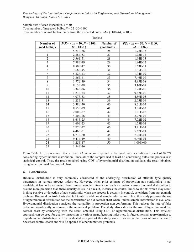
Sample size of each inspection, n = 50 Total number of inspected bulbs, N = 22×50=1100 Total number of non-defective bulbs from the inspected bulbs, M = (1100–64) = 1036

Table 2

Number of good bulbs, x

P(X < x; n = 50, N = 1100, M = 1036 )

Number of good bulbs, x

P(X < x; n = 50, N = 1100, M = 1036 )

0 5.21E-56 26 1.78E-15 1 2.38E-53 27 1.92E-14 2 5.36E-51 28 1.94E-13 3 7.98E-49 29 1.84E-12 4 8.80E-47 30 1.63E-11 5 7.68E-45 31 1.35E-10 6 5.52E-43 32 1.04E-09 7 3.36E-41 33 7.46E-09 8 1.77E-39 34 4.99E-08 9 8.15E-38 35 3.10E-07 10 3.34E-36 36 1.78E-06 11 1.23E-34 37 9.42E-06 12 4.07E-33 38 4.59E-05 13 1.23E-31 39 2.05E-04 14 3.38E-30 40 8.31E-04 15 8.55E-29 41 3.05E-03 16 2.00E-27 42 1.01E-02 17 4.30E-26 43 2.97E-02 18 8.61E-25 44 7.72E-02 19 1.60E-23 45 1.75E-01 20 2.77E-22 46 3.41E-01 21 4.46E-21 47 5.67E-01 22 6.73E-20 48 7.96E-01 23 9.47E-19 49 9.49E-01 24 1.25E-17 50 1.00E+00 25 1.54E-16

From Table 2, it is observed that at least 42 items are expected to be good with a confidence level of 99.7% considering hyperbinomial distribution. Since all of the samples had at least 42 conforming bulbs, the process is in statistical control. Thus, the result obtained using CDF of hyperbinomial distribution validates the result obtained using hyperbinomial 3-σ control chart. 4. Conclusion Binomial distribution is very commonly considered as the underlying distribution of attribute type quality parameters in various product industries. However, when prior estimate of proportion non-conforming is not available, it has to be estimated from limited sample information. Such estimation causes binomial distribution to assume more precision than there actually exists. As a result, it causes the control limits to shrink, which may result in false positive or detection of non-conformity when the process is actually in control, as evident from our example problem. Binomial control charts also fail to utilize additional sample information. Thus, this study proposes the use of hyperbinomial distribution for the construction of 3-σ control chart when limited sample information is available. Hyperbinomial distribution considers the variability in proportion non-conforming. This reduces the rate of false detection significantly as shown in the numerical problem. The study also validates the use of hyperbinomial 3-σ control chart by comparing with the result obtained using CDF of hyperbinomial distribution. This efficient approach can be used for quality inspection in various manufacturing industries. In future, normal approximation to hyperbinomial distribution will be evaluated as a part of this study since it serves as the basis of construction of Shewhart control charts and will be applied to other numerical problems.

165



Acknowledgement The author of this paper is grateful to the Department of Industrial and Production Engineering (IPE), BUET for providing sufficient computational facility to carry out the research. References Hasin, A. A. (2007). Quality control and management. Bangladesh Business Solutions, Dhaka. Montgomery, Douglas C. Introduction to statistical quality control. John Wiley & Sons, 2007. Das, N. (2008). Non-parametric control chart for controlling variability based on rank test. Economic Quality

Control, 23(2), 227-242. Sellers, K. F. (2012). A generalized statistical control chart for over‐or under‐dispersed data. Quality and Reliability

Engineering International, 28(1), 59-65. Feller, W. (2008). An introduction to probability theory and its applications (Vol. 2). John Wiley & Sons. Cheng, S. W. and Xie, H. (2000). Control Charts for Lognormal data, Tamkang Journal of Science and Engineering,

Vol. 3, No. 3, 131-137 Chakraborti, S., Van der Laan, P., & Bakir, S. T. (2001). Nonparametric control charts: an overview and some

results. Journal of Quality Technology, 33(3), 304. Bakir, S. T. (2001, August). Classification of distribution-free quality control charts. In Proceedings of the Annual

Meeting of the American Statistical Association (pp. 5-9). Park, C., Park, C., Reynolds Jr, M. R., & Reynolds Jr, M. R. (1987). Nonparametric procedures for monitoring a

location parameter based on linear placement statistics. Sequential Analysis, 6(4), 303-323. Orban, J., & Wolfe, D. A. (1982). A class of distribution-free two-sample tests based on placements. Journal of the

American Statistical Association, 77(379), 666-672. Shmueli, G., Minka, T. P., Kadane, J. B., Borle, S., & Boatwright, P. (2005). A useful distribution for fitting discrete

data: revival of the Conway–Maxwell–Poisson distribution. Journal of the Royal Statistical Society: Series C (Applied Statistics), 54(1), 127-142.

Jackson, J. E. (1972). All count distributions are not alike. Journal of Quality Technology, Vol 4, No 2, P 86-92, April 1972. 4 Tab, 15 Ref.

Kaminsky, F. C., Benneyan, J. C., Davis, R. D., & Burke, R. J. (1992). Statistical control charts based on a geometric distribution. Journal of Quality Technology, 24(2).

Joekes, S., & Barbosa, E. P. (2013). An improved attribute control chart for monitoring non-conforming proportion in high quality processes. Control Engineering Practice, 21(4), 407-412.

Fisher, S. R. A., & Cornish, E. A. (1960). The percentile points of distributions having known cumulants. Technometrics, 2(2), 209-225.

Haldar, A., & Mahadevan, S. (2000). Probability, reliability, and statistical methods in engineering design. John Wiley.

Haldar, A. (1982). Statistical and Probabilistic Methods in Geomechanics. In Numerical Methods in Geomechanics (pp. 473-504). Springer, Dordrecht

166



Appendix Derivation of Mean and Variance for Hyperbinomial Distribution: We know, the PMF of hyperbinomial distribution is

( ) of | of , for 0,1, 2,...., , and 1X

m x N n m xm n x

P x n m N x n m NN n

n

+ + − − − = = ≤

+ +

Since, ,p pr p r

= −

som x m x

m x+ +

=

, we can write,

( ) of | of , for 0,1, 2,...., , and 1X

m x N n m xx n x

P x n m N x n m NN n

n

+ + − − − = = ≤

+ +

Now, ( )

( )( )

( )( )

!! !

! 11 ! ! 1

x m xm xx

x x m

x m x mx x m m

++ =

+ +

= ×− +

( ) ( ) ( )( ) ( )

( ) ( ) ( )( )

1 1 1 !1 ! 1 !

1 11

1

m m xx m

m xm

m

+ + + − =− +

+ + −= + +

Again, ( )

( )( ) ( )

( ) ( )( )( )

( ) ( ) ( )( )

1 !1! 1 !

1 1 1 ! 21 ! 1 ! 2

2 1 1 11

N nN nn n N

N n Nn n N N

N N nnn

+ ++ + = +

+ + − + + = ×− + +

+ + + − += −

167



Mean of hyperbinomial distribution can be found as follows:

( )

( ) ( ) ( )( )

( ) ( ) ( ) ( )( ) ( )

( ) ( ) ( )( )

0

0

1

of | of

1

1 11

1

1 1 1 11 1

1 1 12

1

h

X Xx

h

x

h

x

xP x n m N

m x N n m xx n x

xN n

n

m xm

m

N n m xn x

N nNnn

µ=

=

=

=

+ + − − − =

+ + + + −

+ × + + + − − + − − − − − =

+ + − ++ −

∑

∑

∑

( )( )

( ) ( )( )

( ) ( ) ( ) ( )( ) ( )

( ) ( )( )

1

1 11

1 1 1 11 11

2 1 1 1

1

h

x

m xm

N n m xn xn m

N N nn

=

+ + −× +

+ + − − + − − − − −+ =

+ + + − + −

∑

Since the expression inside the summation symbol is analogous to the PMF of hyperbinomial distribution, the summation over the full range of x must be equal to 1. So we can write:

( )( )X

1

2n m

Nµ

+=

+

168



Variance of hyperbinomial distribution can be found as follows:

( ) ( ) ( )

( ) ( )

( ) [ ] ( )( ) [ ] ( )( )( ) ( ) ( )

( )

22

2

2

0

0

Var E E

E 1 E

E 1 E E

E 1 E 1 E

1 of | of 1

1

1

h

X X Xx

h

x

X X X

X X X X

X X X X

X X X X

x x P x n m N

m x N n m xx x

x n xN n

n

µ µ=

=

= −

= − + −

= − + −

= − + −

= − + −

+ + − − − − =

+ +

∑

∑

( ) 1X Xµ µ+ −

Now,

( ) ( )( )

( )( )( )( )

( )( )( )( )

1 !1

! !

1 ! 1 21 2 ! ! 1 2

x x m xm xx x

x m x

x x m x m mx x x m m m

− ++ − =

− + + +

= ×− − + +

( ) ( )( ) ( ) ( )( )

( )( ) ( ) ( )( )

2 2 !1 2

2 ! 2 !

2 21 2

2

m xm m

x m

m xm m

m

+ + − = × + +− +

+ + −= + + +

Again,

( )( )

( ) ( )( )( ) ( )

( )( )( )( )

( )( )( )

( ) ( )( ) ( )

( )( )( )

( ) ( )

1 !1! 1 !

2 2 1 ! 2 31 2 ! 1 ! 2 3

2 2 1 !2 31 2 ! 3 !

2 3 2 2 11 2

N nN nn n N

N n N Nn n n N N N

N nN Nn n n N

N N N nn n n

+ ++ + = +

+ + − + + + = ×− − + + +

+ + − ++ + = ×− − +

+ + + + − +=

− −

( )( )

( )

0

1Var

1

1

h

x

X X

m x N n m xx x

x n xX

N nn

µ µ

=

+ + − − − − ∴ =

+ + + −

∑

169



Since the term ( ) ( )

( )( ) ( ) ( ) ( )

( ) ( )( ) ( )

−

+−++

−−−

−−+−−++

+

−++

2122

222222

222

nnN

xnxmnN

mxm

is analogous to the PMF of hyperbinomial distribution, summation of this term over full range of x must be equal to 1. Hence,

( ) ( )( )( )( )( ) ( )

( )( )( )( )( )

( )( )

( )( )

( )[ ]( ) ( )32

22321211

21

32211

1132

211Var

2

2

+++−+−+−++

=

++

−++

+++

++−=

−+×++

++−=

NNmNnnNnmNmNmn

Nmn

Nmn

NNmmnn

NNmmnnX XX µµ

( )( ) ( ) ( )( )

( ) ( ) ( ) ( )( ) ( )

( )( )( )

( ) ( )( )

( )( )( )( )( )

( ) ( )( )

( ) ( ) ( ) ( )( ) ( )

( ) ( )( )

2

2

2 2 2 22 22 2

1 2 12 2 3 2 2 1

1 2

2 2 2 2 2 22 2 21 1 2

12 3 2 2 1

2

h

X Xx

h

X Xx

N n m xn xm x

m mm N N N n

n n n

m x N n m xm n xn n m m

N N N nn

µ µ

µ µ

=

=

+ + − − + − − − − − + + − = + + × + − + + + + + − + − −

+ + − + + − − + − − + − − −− + + = × + −

+ + + + − + −

∑

∑

Now,

( ) ( )( )

( )( )( )( )

( )( )( )( )

( ) ( )[ ]( ) ( ) ( )( )

( )( ) ( ) ( )( )

+

−++++=

++×+−−++

=

++++

×−−+−

=

+−=

+−

222

21

21!2!2

!222121

!!21!1

!!!11

mxm

mm

mmmx

xmmmmm

mxxxxmxx

xmxmxx

xxm

xx

( )

( )( ) ( )[ ]( )( ) ( )

( )( )( )( )

( )( )( )

( ) ( )[ ]( ) ( )

( )( )( )

( ) ( )

−

+−++−

++=

+−+−++

×−

++=

++++

×+−−+−++

=

+++

=

++

2122

132

!3!2!122

132

3232

!1!21!122

!1!!11

nnN

nnNN

NnnN

nnNN

NNNN

NnnnnN

NnnN

nnN

170



( )( )

( )

( )( ) ( ) ( )( )

( ) ( ) ( ) ( )( ) ( )

( )( )( )

( ) ( ) ( )

( )( )( )( )( )

( ) ( )( )

( ) ( ) ( ) ( )( ) ( )

( ) ( ) ( )XX

h

x

XX

h

x

XX

h

x

nnN

xnxmnN

mxm

NNmmnn

nnN

nnNN

xnxmnN

mxm

mm

nnN

xnxmnN

xxm

xxX

µµ

µµ

µµ

−+

−

+−++

−−−

−−+−−++

+

−++

++++−

=

−+

−

+−++−

++

−−−

−−+−−++

+

−++++

=

−+

++

−

−−+

+−

=∴

∑

∑

∑

=

=

=

1

2122

222222

222

32211

1

2122

132

222222

222

21

11

1Var

2

2

0

Since the term

( ) ( )( )

( ) ( ) ( ) ( )( ) ( )

( ) ( )

−

+−++

−−−

−−+−−++

+

−++

2122

222222

222

nnN

xnxmnN

mxm

is analogous to the PMF of hyperbinomial distribution, summation of this term over full range of x must be equal to 1. Hence,

( ) ( )( )( )( )( ) ( )

( )( )( )( )( )

( )( )

( )( )

( )[ ]( ) ( )32

22321211

21

32211

1132

211Var

2

2

+++−+−+−++

=

++

−++

+++

++−=

−+×++

++−=

NNmNnnNnmNmNmn

Nmn

Nmn

NNmmnn

NNmmnnX XX µµ

Biography / Biographies Shourav Ahmed is a Lecturer in the Department of Industrial and Production Engineering (IPE) at Bangladesh University of Engineering and Technology (BUET), Dhaka, Bangladesh. He earned his B.Sc. and M.Sc. degrees in Industrial and Production Engineering from BUET, Dhaka, Bangladesh in 2015 and 2018, respectively. He has completed research projects with Nestle, National Polymer and Walton. His research interests include quality management, supply chain management, micro/nano fabrication, multidisciplinary design optimization, uncertainty quantification, etc. He is an esteemed member of IEB, ORCA, and AIPE.

Gulam Kibria is a Lecturer in the Department of IPE at BUET, Dhaka, Bangladesh. He earned his B.Sc. and M.Sc. degrees in Industrial and Production Engineering from BUET, Dhaka, Bangladesh in 2015 and 2018, respectively. His research interests include operations management, operations research and decision analysis, multidisciplinary system analysis, uncertainty and risk management, etc.

Kais Zaman is a professor in the Department of Industrial and Production Engineering (IPE) at Bangladesh University of Engineering and Technology (BUET), Dhaka, Bangladesh. Currently, he is also the head of the department. He earned his B.Sc. and M.Sc. degrees in Industrial and Production Engineering from BUET, Dhaka, Bangladesh in 2003 and 2005, respectively. He also earned his M.Sc. and Ph.D. degrees in Reliability and Risk Engineering and Management from Vanderbilt University in 2010. His research interests include artificial intelligence and machine learning, operations research and decision analysis, uncertainty and risk management, etc. He has publications in numerous prestigious journals and conferences.

171

a new approach to constructing control chart for …ieomsociety.org/ieom2019/papers/62.pdfzahir...

Documents