1

A New Approach of Exploiting Self-Adjoint MatrixPolynomials of Large Random Matrices for

Anomaly Detection and Fault LocationZenan Ling1,Robert C. Qiu1,2, IEEE Fellow, Xing He1, Lei Chu1

Abstract—Synchronized measurements of a large power gridenable an unprecedented opportunity to study the spatial-temporal correlations. Statistical analytics for those massivedatasets start with high-dimensional data matrices. Uncertaintyis ubiquitous in a future’s power grid. These data matricesare recognized as random matrices. This new point of view isfundamental in our theoretical analysis since true covariancematrices cannot be estimated accurately in a high-dimensionalregime. As an alternative, we consider large-dimensional samplecovariance matrices in the asymptotic regime to replace thetrue covariance matrices. The self-adjoint polynomials of large-dimensional random matrices are studied as statistics for bigdata analytics. The calculation of the asymptotic spectrum dis-tribution (ASD) for such a matrix polynomial is understandablychallenging. This task is made possible by a recent breakthroughin free probability, an active research branch in random matrixtheory. This is the very reason why the work of this paperis inspired initially. The new approach is interesting in manyaspects. The mathematical reason may be most critical. The real-world problems can be solved using this approach, however.

Index Terms—Data-driven, high-dimensional data, randommatrix theory, free probability, anomaly detection, fault location

I. INTRODUCTION

Among challenges for big data analytics towards grid mod-ernization, data-driven approach and data utilization are ofgreat significance in power system operation in smart grids [1].Current power systems are huge in size and complex in topol-ogy. Model-based methods can not always meet the real-lifeneeds when assumptions and simplifications are prerequisitesfor these mechanism models. Massive datasets are accessible,however, when the operation of the power system is monitoredby a large number of sensors such as phase measuurment units(PMUs). For instance, China has deployed 1717 PMUs as of2013 [2] and there are about 500 PMUs installed by July2012 in America [3].

This work was partly supported by NSF of China No. 61571296 and (US)NSF Grant No. CNS-1619250.

c© 20xx IEEE. Personal use of this material is permitted. Permission fromIEEE must be obtained for all other uses, in any current or future media,including reprinting/republishing this material for advertising or promotionalpurposes, creating new collective works, for resale or redistribution to serversor lists, or reuse of any copyrighted component of this work in other works.

1 Department of Electrical Engineering, Center for Big Data andArtificial Intelligence, State Energy Smart Grid Research and Devel-opment Center, Shanghai Jiaotong University, Shanghai 200240, China.(e-mail: ling zenan@163.com; rcqiu@sjtu.edu.cn; hexing hx@126.com;leochu@sjtu.edu.cn).

2 Department of Electrical and Computer Engineering, Tennessee Techno-logical University, Cookeville, TN 38505, USA. (e-mail:rqiu@tntech.edu).

The synchronized measurements of a large power gridenable the joint modeling of temporal statistical propertiesacross the spatial nodes. The spatial-temporal couplings poseopportunities and challenges. Towards this goal, random ma-trix theory (RMT) is used for data analysis first in [4]. RMTstarts in the early 20th century. Due to the increase in thedimensionality of collected datasets, RMT has been commonlyused for considering problems regarding the behavior ofeigenvalues of large dimensional random matrices in physics,finance, wireless communication, etc [5, 6].

Due to the large size of datasets, randomness or uncertaintyis at the heart of data modeling and analysis in a complex, largepower gird when rapid fluctuations in voltages and currentsare ubiquitous. Often, these fluctuations exhibit some certain(or deterministic) distribution properties [7]. Our approachexploits the massive datasets across the large grid that aredistributed in both spatially and temporally. Random matrixtheory (RMT) appears very natural for the problem at hand.In a random matrix of size CN×T , we use N variables to rep-resent the spatial nodes. For the i-th node where i = 1, ..., N ,there are T observations to represent the temporal samplest = 1, ..., T. When the number of nodes N and data samples Tare large, very unique mathematical phenomenon occurs suchthat power mathematical tools such as free probability [5] canbe exploited to develop big data analytics for joint spatial-temporal datasets. This is the central purpose of this paper.

Free probability is a powerful tool for solving randommatrix problems, such as additive and multiplicative free con-volution. Based on free probability theory, asymptotic limits ofthe testing functions (free self-adjoint matrix polynomials), canbe obtained numerically through certain algorithms. Closedform expressions exist only for some simple matrix polyno-mials. The obtained asymptotic limits provide the rigorousbounds in mathematics which can help distinguish signalsand noise in grid data. The anomaly detection is conductedthrough hypothesis testing and an indicator for fault locationis designed using some mathematical tricks.

A. Contributions of Our Paper

This paper is built upon our previous work [4, 8–10] inthe last several years. Motivated for machine learning frommassive datasets, our line of research is based on the mod-ern high-dimensional statistics where RMT is central to thisparadigm. The contributions of this paper can be summarizedas follows:

arX

iv:1

802.

0350

3v1

[st

at.A

P] 1

0 Fe

b 20

18

2

1) The aim of this paper is to exploit the polynomialsof large random matrices in the context of big dataanalytics for a large power grid. To our best knowledge,this attempt is for the first time. This analysis is madepossible by a recent breakthrough [11, 12] in the literatureof mathematics. Our result represents one of the firstapplications of these algorithms in engineering.

2) Using the new analytic tool [11, 12] from free probabilitytheory, we are able to distinguish the noise and signalsfrom grid data with provable mathematics guarantees. Itis natural to conduct anomaly detection by hypothesistesting.

3) Both linear and nonlinear polynomials of large randommatrices can be handled in this new framework [11, 12].Simulations demonstrate that compared with the linearcases, nonlinear cases perform better in reducing the falsealarm probability.

4) Based on certain new algorithms developed in this paper,an indicator for fault location is proposed and validatedto be valid by simulations and real-world cases.

B. Related Work

There are numerous researches on data driven methods formodeling and analysing large power systems. Le, Chen andKumar [13] propose a linearized analysis method for earlyevent detection using partial least squares estimation. Limand DeMarco [7, 14] propose a singular value decomposi-tion (SVD)-based voltage stability assessment from principalcomponent analysis (PCA). Both methods in the above arePCA related and the selection of the eigenvalues has a crucialinfluence. Lim et al select the largest eigenvalue and Xieet al [15] adopt the method of the threshold of cumulativevariance proportion. Their common disadvantage is that thepre-defined threshold depends on the experience without theconsideration of the statistical characteristic of the grid data,so the redundancy or loss of information is unavoidable.

Also, along with the new wave of deep learning, someNeural Network based methods are proposed. With powerfulmodeling ability of neural networks, Eltigani [16] realizeassessing the transient stability. Zhou [17] present a method forlong-term voltage stability monitoring based on Artificial Neu-ral Network which requires training before online deployment.However, the training speed of networks slows down withthe scale-up of the system and increase of training samples.Moreover, the high quality of the sampling data is crucialfor the neural network’s generalization ability which is notpractical in current power system.

This paper is organized as follows. Section II establishesthe random matrix model for the power grid as the basisof this paper. Section III proposes the anomaly detectionmethod from the way of hypothesis testing and an indicatorfor fault location. Section IV provides a brief introduction ofthe algorithm for obtaining the asymptotic spectral distributionof free self-adjoint polynomial which is essential for ouranalytical framework. In Section V, numerical case studiesvalidate our methods with simulation data and real-world data.In Section VI, the estimation of signal strength is discussed

under the linear assumption. Conclusion and further directionof this research are given in Section VII. For the sake ofsimplicity, some details and the supplementary materials aredeferred to the Appendix.

II. RANDOM MATRIX MODEL AND DATA PROCESSING FORPOWER GRID

A. Random Matrix Model for Power Grid

Following [4, 9], the power flow equations, which definethe equilibrium operating condition of a power system, can bewritten as:[

∆P∆Q

]= J

[∆θ∆V

]=

[∂P (θ,V )

∂θ∂P (θ,V )∂V

∂Q(θ,V )∂θ

∂Q(θ,V )∂V

] [∆θ∆V

](1)

where P,Q, V, θ denotes the active power, the reactive power,the voltage phase angle and the voltage amplitude respectively.

To characterize the role of each block of the Jacobianmatrix, denote:

H = ∂P (θ,V )∂θ , N = ∂P (θ,V )

∂V

K = ∂Q(θ,V )∂θ , L = ∂Q(θ,V )

∂V

(2)

Then, taking the inverse of the Jacobian matrix J in (1)leads to (3), providing the desired input-output relationship,[

∆θ∆V

]=

[M −MNL−1

−L−1KM L−1 + L−1KMNL−1

] [∆P∆Q

](3)

where M = (H −NL−1K)−1.Therefore, under the situation that Q is relatively constant,

the model between V and P is obtained as:

∆V = Ξ∆P (4)

with Ξ = −L−1KM .Considering T random vectors observed at time i = 1, ..., T,

a random matrix is formed as follows:

[∆V1, · · · ,∆VT ] = [Ξ1∆P1, · · · ,ΞT∆PT ] . (5)

It is worth noting that only voltage magnitude of PMU datais used. The voltage magnitude are more sensitive to topologychange than phase angle and they remain relatively stable innormal operating condition [14]. Without dramatic topologychanges, rich statistical empirical evidence indicates that theJacobian matrix J keeps nearly constant, so does Ξ. Thus (5)is rewritten as:

V = ΞPN×T (6)

where V = [∆V1, · · · ,∆VT ], Ξ = Ξ1 = · · · = ΞT , andP = [∆P1, · · · ,∆PT ] . Here V and P are random matrices.To model the fast time scale stochastic variation in a load,we assume that P is a random matrix with Gaussian randomvariables as its entries, following [4, 9].

3

B. Data Processing Method

The sampling data matrix V of real power grid is alwaysnon-Gaussian, so a normalization procedure in [4] is adoptedto conduct data preprocessing. Meanwhile, a Monte Carlomethod is employed to estimate the empirical spectral dis-tribution (ESD) of raw grid data according to the asymptoticproperty theory.

The data processing procedure above is organized as fol-lowing steps in Algorithm 1. The parameter N denotes thenumber of buses and T denotes the sampling period. Notethat η is extremely small, e.g. η = 10−5 and M is set to 10in our simulation cases.

Algorithm 1Input:

The sample data matrices: V;The number of repetition times: M (10 is enough);The size of V: N,T ;The variance of the small white noise εN×T : η;

1: for i ≤M do2: Add small white noises εN×T to the sample data matrix

V = V + εN×T ;3: Standardize V , i.e. mean=0, variance=1;4: Calculate the sample covariance matrices: Σ = VV′

/T ;5: Calculate the eigenvalues of Σ;6: end for7: Calculate the empirical spectral distribution of Σ;

Output:The histogram of the ESD of Σ .

C. Validation of Proposed Model

Marchenko-Pastur Law (M-P Law) [18], a basic theoremin random matrix theory, is introduced to verify the randommatrix model for power grid.

Theorem II.1 (M-P Law [18]). Let X = {xi,j} be a N ×T random matrix whose entries with the mean µ = 0 andthe variance σ2 <∞, are independent identically distributed(i.i.d). As N,T −→∞ with the ratio c = N/T ∈ (0, 1].

Σ =1

TXXH ∈ CN×N (7)

is the corresponding sample covariance matrix. Then, theasymptotic spectral distribution of Σ is given by:

µ′(x) =

{1

2πxσ2

√(b− x)(x− a) if a ≤ x ≤ b

0 otherwise(8)

where a = σ2(1−√c)2, b = σ2(1 +

√c)2. Here, Σ is called

Wishart matrix.

According to Algorithm 1, we obtain the ESD of the samplecovariance matrix Σ of real-world datasets for 34 PMUs. TheV is collected in normal operation.

As illustrated in Fig 1, the histogram of the ESD ofΣ coincides with the M-P Law. Although the asymptoticconvergence is considered under infinite dimensions, i.e.,N → ∞, T → ∞ but N/T → c ∈ (0, 1) , the asymptotic

results are fairly accurate for moderate matrix sizes such asN = 10s. It effectively explains why RMT is practical for thereal-world datasets in a power grid.

Fig. 1: Histogram of the empirical spectral distribution of thecovariance of 34-PMU data collected in normal operation. Thered curve represents the M-P Law.

III. ANOMALY DETECTION AND FAULT LOCATION

A. Hypothesis Testing For Anomaly Detection

Based on the random matrix model for power gird in II-A,the problem of anomaly detection is formulated in terms ofthe hypothesis testing :∣∣∣∣ H0 : Σ1 = Σ0

H1 : Σ1 6= Σ0(9)

where Σ0 is the sample covariance matrix of the grid datacollected in normal operation and Σ1 is the sample covariancematrix of the grid data for abnormal operation. This problemis a matrix hypothesis testing [5, 6]. Test statistics are centralto hypothesis testing.

In this paper P (Σ1,Σ0) is adopted as test statistics. Here,P is a self-adjoint polynomial of large random matrices, i.e.P = PH . The P (Σ1,Σ0) measures the difference betweentwo sample covariance matrices.

Theorem III.1 (The self-adjoint matrix polynomial of largeHermitian random matrices [12]). Let ΣN = (Σ

(N)1 , ...,Σ

(N)p )

be a family of independent, normalized N × N Wishartmatrices. Assume that for every Hermitian matrix PN of theform

PN = P (ΣN ) (10)

where P is a free self-adjoint matrix polynomial, we have withprobability one that: 1. The empirical spectral distribution ofa free self-adjoint matrix polynomial PN converges weakly toa compactly supported µ on the real line as N goes to infinity.

2. For any ε > 0, almost surely there exits N0 such thatfor all N > N0, Sp(PN ) ⊂ Supp(µ) + (−ε, ε), where ’Sp’means the spectrum and ’Supp’ means the support.

Theorem III.1 implies that if H0 is true, the ESD ofP (Σ1,Σ0) will coincide with a theoretical curve1, i.e. theasymptotic spectral distribution (ASD) of P . Besides, noeigenvalue exits outside of the support of the theoretical curve.

1This curve can be calculated by a certain algorithm. See Section III fordetails.

4

In this paper, the eigenvalues outside of the support arecalled outliers.

According to Theorem III.1, the proposed detection methodis summarized as follows:

1) Calculate Σ0 and Σ1 from the sample data with thepreprocessing method stated in Algorithm 1.

2) Compare the theoretical curves corresponding with theESDs of different matrix polynomials P (Σ1,Σ0).

3) Anomaly detection is conducted: if outlier exists, H0 willbe rejected, i.e. signals exist in the system.

Based on the hypothesis testing (9), we propose a statisticindicator denoted by

s =

∑λk∈outliers

λk∑λk /∈outliers

λk. (11)

The function of s is similar to the signal-to-noise ratio.Notice that our proposed detection method is quite sensitive

to the signal even if the signal is extremely weak [19]. Inorder to reduce the false alarm probability, it is necessary forthe values of s of the normal and the abnormal load variationto be different. So the choice of the polynomial functions iscrucial.

In this paper, we study two typical self-adjoint matrix poly-nomials. The first one is the multivariate linear polynomial:

P1(Σ0,Σ1) = Σ1 − Σ0. (12)

The second one is the multivariate nonlinear polynomial:

P2(Σ0,Σ1) = (Σ1 − Σ0)2. (13)

Here, both Σ0 and Σ1 are the sample covariance matrices.The simulation results in Section V will show that the per-formance of the nonlinear polynomial is much better than thelinear one.

It is difficult to obtain the ASD of free self-adjoint polyno-mials P1 and P2. Fortunately, the recent breakthrough [11, 12]in free probability in random matrix theory has made thispossible. To make the paper self-contained, the algorithm forcalculating the ASD of P is introduced briefly in Section III.

B. Fault Location

In this subsection, we investigate the fault location basedon the proposed anomaly detection method in III-A. Since theselected polynomials P (Σ0,Σ1) are real and symmetric, thefollowing equations

P = v

λ1

. . .λN

u, (14)

Pvk = λkvk (15)

hold. Here, v,u denote the left and right eigenvector matrix;λk is an eigenvalue of P (Σ0,Σ1) and it indicates the energyof the corresponding eigenvector vk.

For the element Pij in P , the derivative of (15) leads to thefollowing:

dP

dPijvk + P

dvkdPij

=dλkdPij

vk + λkdvkdPij

. (16)

Left multiply (16) by uTk . Note that ukT vk = 1 and uT = vand we have

dλkdPij

= ukT dP

dPijvk. (17)

Let ψ = dPdPij

. Obviously, only ψij = 1 and other elementsof ψ equal to zero. So (17) is simplified as:

dλkdPij

= ukjvik. (18)

Finally, the contribution of the i-th row to the eigenvalueλk is obtained by:

T∑j=1

(dλkdPij

)2

=

T∑j=1

(ukjvik)2

=vik2T∑j=1

(ukj)2

=vik2. (19)

In the work of Lim et al [14], the singular vector corre-spondingto the largest singular value is used to conduct faultlocation. The simulation results in [14] show that the singularvector tells which buses are contributing to the correspondingsingular value.

For the hypothesis testing in III-A, not only the largesteigenvalue of the covairance matrix but also the outliersare viewed as the “signals”. This observation inspires us toimprove Lim’s method by studying those eigenvectors corre-sponding to outliers. In particular, we design a new locationindicator denoted by

Li =

∑λk∈outliers

λkv2ik∑

λk∈outliers

λk, (20)

to quantify each bus’s contribution to the anomaly. Since thatv2ik∈ [0, 1] and

∑i

v2ik = 1, obviously,

∑i

∑λk∈outliers

λkv2ik =

∑λk∈outliers

λk (21)

Thus, Li ∈ (0, 1] and∑i

Li = 1. From the above, Li is a

reasonable indicator that measures the correlation between thei-th bus and the load variation. The location (denoted as loc)of the most sensitive bus can be expressed as

loc = arg max︸ ︷︷ ︸i∈(1,...,N)

Li. (22)

The simulation results in V-C show that our method performsbetter than Lim’s work [14] in the fault location task.

All the eigenvalues outside the support of the theoreticalcurve are considered. The functions of P (Σ0,Σ1) play arole of machine learning that classify between the noise andsignals. Outliers are remained as the useful signals for anomalydetection and fault location.

5

IV. THE ASYMPTOTIC SPECTRAL DISTRIBUTION OF FREESELFADJIONT POLYNOMIAL

In this section, we study the asymptotic spectral distribution(ASD) of P1 and P2, on the premise that both Σ0 and Σ1 areWishart matrices.

A. The ASD of P1

For obtaining the ASD of P1, we introduce the operator-valued setting [12] briefly. Let A be a unital algebra and B ⊂A be a subalgebra containing the unit. A linear map E : A →B is a conditional expectation. For a random variable x ∈A, we define the operator-valued Cauchy transform: G(b) :=E[(b− x)

−1](b ∈ B) for which (b− x) is invertible in B. Let

H+(B) := {b ∈ B|=b > 0}. In the following theorem [11],we will use the notation h(b) := 1

G(b) − b.

Theorem IV.1 ([11]). Let x and y be self-adjoint operator-valued random variables free over B. Then there exists aFrechet analytic map ω : H+(B)→ H+(B) so that•=ωj(b) ≥ =b for all b ∈ H+(B), j ∈ {1, 2}•Gx(ω1(b)) = Gy(ω2(b)) = Gx+y(b)Moreover, if b ∈ H+(B) , then ω1(b) is the unique fixed

point of the map. fb : H+(B)→ H+(B), fb(ω) = hy(hx(ω)+b) + b, and ω1(b)= lim

n→∞fbon(ω) for any ω ∈ H+(B), where

fonb means the n-fold composition of fb with itself. Same state-ments hold for ω2(b), with replaced by ω → hx(hy(ω)+b)+b.

Theorem IV.2 (Stieltjes inversion formula [20]). For any openinterval I = (a, b) , such that neither a nor b are atoms forthe probability measure µ, the inversion formula

µ(I) = − 1

π

∫I

=(Gu(x+ iy))dx

holds.

Theorem IV.1 provides an iterative algorithm to compute theoperator-valued Cauchy transform of P1. Then, the ASD of P1

is easily obtained through the Stieltjes inversion formula.

B. The ASD of P2

The ASD of P2 is obtained by linearizing the nonlinearpolynomial. Through Anderson’s linearation trick [21], wehave a procedure that leads finally to an operator:

Lp = c⊗ 1 + b0 ⊗ Σ0 + · · · bn ⊗ Σn.

In the case of P2,

LP2=

0 Σ1 − Σ0Σ1−Σ0

2Σ1 − Σ0 0 −1

Σ1−Σ0

2 −1 0

Therefore, LP2

can be easily written in the form of LP2=

c ⊗ 1 + b0 ⊗ Σ0 + b1 ⊗ Σ1, where c =

0 0 00 0 −10 −1 0

,

b0 =

0 −1 − 12

−1 0 0− 1

2 0 0

, b1 =

0 1 12

1 0 012 0 0

.

Theorem IV.3 ([11]). Consider that p ∈ C < X1, . . . , Xn >that has a self-adjoint linearization

Lp = b0 ⊗ 1 + b1 ⊗X1 + · · · bn ⊗Xn.

Let

Λ(z) :=

z 0 · · · 00 0 · · · 0...

.... . .

...0 0 · · · 0

for all z ∈ C.

Then, for each z ∈ C+ and all small enough ε > 0 , theoperators z − P ∈ A and Λε(z) − LP ∈ MN (C) ⊗ A areboth invertible and

GP (z)=limε→0

[GLP(Λε(z))]1,1 for all z ∈ C+

holds.

Theorem IV-B illustrates the relationship between theCauchy transform of P2 and LP2 . Thus, the nonlinear problemis turned into the linear problem which is solved in IV-A.

Finally, the ASD of P2 is obtained through the application ofTheorem IV.1 and the Stieltjes inversion formula. See specificprocedures of the algorithm in Appendix A.

V. CASE STUDIES

The proposed method is tested with the simulated datagenerated from IEEE 118-bus and a Polish 2383-bus system,respectively. Detailed information of the system is referredto the case118.m and case118.m in Matpower package andMatpower 4.1 User’s Manual [22].

In subsection V-A, V-B and V-C, the proposed methodis tested with simulated data in the standard IEEE 118-bussystem, as shown in Fig. 10 in Appendix B. The resultsgenerated form the Polish 2383-bus system are deferred tothe Appendix C.

In subsection V-D, the fault location method is validated byreal-world 34-PMU data.

For Cases 1-3, set the sample dimension, i.e. the numberof buses, as N = 118. The spectral density distribution offree adjoint polynomial can be obtained through the algorithmin Section III as long as N ≤ T . Meanwhile, the sampledimension N is required to be large enough to guaranteethe accuracy of results in the proposed asymptotic theory ofeigenvalue distributions. Therefore, in Cases 1-3 , we set thesample length to be equal to N , i.e. T = 118, c = T/N = 1and select six sample voltage matrices presented in Tab. I. Theload variation is shown in Fig. 11 in Appendix B.

TABLE I: System status and sampling data

Cross Section (s) Sampling (s) DescripitonC0 : 118− 900 V0 : 100 ∼ 217 Reference, no signalC1 : 901− 1017 V1 : 850 ∼ 967 Existence of a step signal for

Bus 22C2 : 1918−2600 V2 : 2200 ∼ 2317 Steady load growth for Bus 22C3 : 3118−3790 V3 : 3300 ∼ 3417 Steady load growth for Bus 52C4 : 3908−4100 V4 : 3900 ∼ 4017 Chaos due to voltage collapseC5 : 4118−5500 V5 : 4400 ∼ 4517 No signal

*We choose the temporal end edge of the sampling matrix as the markedtime for the cross section. E.g., for V0 : 100 ∼ 217, the temporal label is217 which belong to C0 : 118− 800.

6

Power grid operates with only white noises during 0 s to 900s; we choose sampling matrix V0 as the reference. Similarly,we mark other kinds of system operation status as C1–C5, andchoose their relevant sampling matrix V1–V5 for the test.

A. Case 1: Anomaly Detection with the Multivariate LinearPolynomial P1

We conduct anomaly detection using Vi (i ≥ 1) and thereference matrix V0 through the proposed hypothesis testing(9). Note that covariance matrix Σi is generated from Vi bythe preprocessing in II-B. Then, we choose the multivariatelinear polynomial

P1(Σ0,Σi) = Σi − Σ0, i = 1, 2, 3, 4, 5

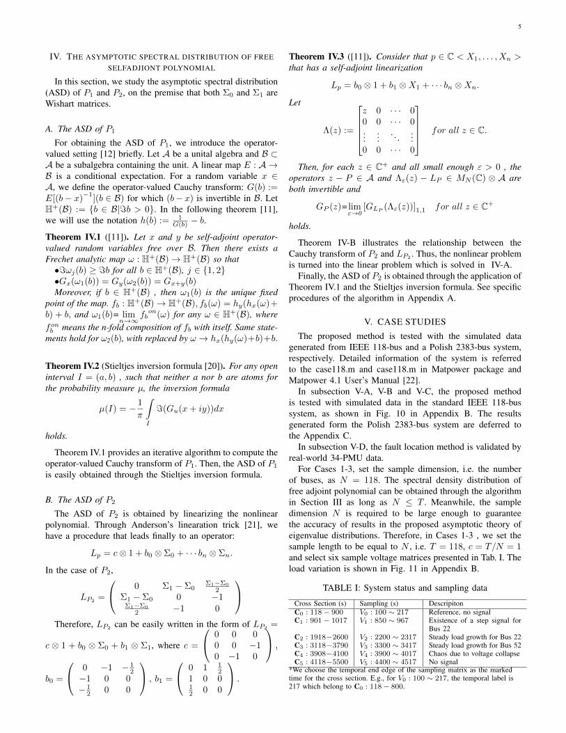
to conduct this detection. Simulation results are shown inFig. 2. The red curve represents the ASD of P1 obtained byTheorem IV.1. The ESD histogram of P1(Σ0,Σi) is plotted byusing Algorithm 1. Outliers are highlighted by ellipses. Thevalues of s defined in (11) in C1–C5 are presented in Tab. II.

1) For Fig. 2(a)-(d), the actual histograms agree withthe theoretical curve very well except a few spikes (calledoutliers); (e): for the white noise case, there are no outliers,as expected by the theory.

2) Sort by the values of s: C5 < C2 < C3 < C1 < C4.From result 1), we observe that this method distinguishes

the signals from the white noise successfully. Result 2) impliesthat the size of outliers indicates the strength of the signals.

However, the discrimination between the ramp signals andthe step signals are not very obvious. See Table II for details.To deal with this disadvantage, a direct approach is to increasethe sensitivity for a given signal-to-noise ratio. In particular,a nonlinear polynomial P2 is adopted.

TABLE II: The values of s in C1–C5

CrossSection

Description s

C1 Existence of a step signal 0.1096C2 Steady load growth 0.0357C3 Steady load growth 0.0609C4 Chaos due to voltage collapse 0.4219C5 No signa 0.000

B. Case 2: Anomaly Detection with the Multivariate Nonlin-ear Polynomial P2

In Case 2, the process is similar to V-A except that the teststatistic function is replaced with

P2(Σ0,Σi) = (Σi − Σ0)2, i = 1, 2, 3, 4, 5

which is a multivariate nonlinear polynomial in two matrices.This is the simplest second-order polynomial. Of course, wecan study higher orders that will be left for the work in a nextpaper.

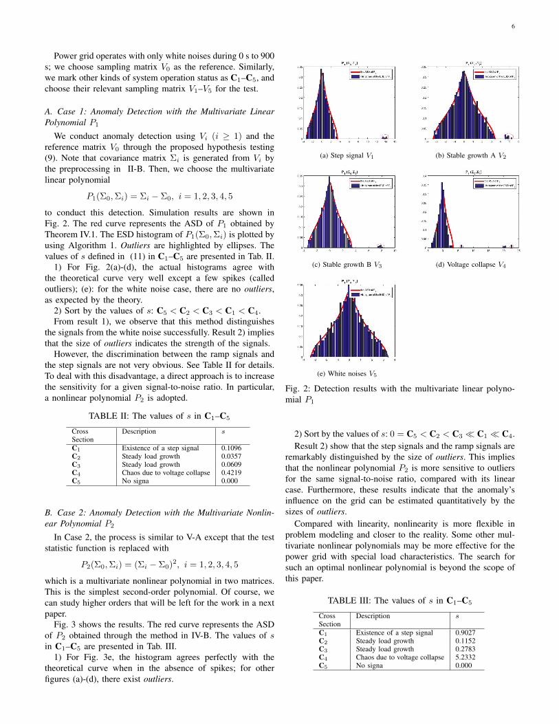
Fig. 3 shows the results. The red curve represents the ASDof P2 obtained through the method in IV-B. The values of sin C1–C5 are presented in Tab. III.

1) For Fig. 3e, the histogram agrees perfectly with thetheoretical curve when in the absence of spikes; for otherfigures (a)-(d), there exist outliers.

(a) Step signal V1 (b) Stable growth A V2

(c) Stable growth B V3 (d) Voltage collapse V4

(e) White noises V5

Fig. 2: Detection results with the multivariate linear polyno-mial P1

2) Sort by the values of s: 0 = C5 < C2 < C3 � C1 � C4.Result 2) show that the step signals and the ramp signals are

remarkably distinguished by the size of outliers. This impliesthat the nonlinear polynomial P2 is more sensitive to outliersfor the same signal-to-noise ratio, compared with its linearcase. Furthermore, these results indicate that the anomaly’sinfluence on the grid can be estimated quantitatively by thesizes of outliers.

Compared with linearity, nonlinearity is more flexible inproblem modeling and closer to the reality. Some other mul-tivariate nonlinear polynomials may be more effective for thepower grid with special load characteristics. The search forsuch an optimal nonlinear polynomial is beyond the scope ofthis paper.

TABLE III: The values of s in C1–C5

CrossSection

Description s

C1 Existence of a step signal 0.9027C2 Steady load growth 0.1152C3 Steady load growth 0.2783C4 Chaos due to voltage collapse 5.2332C5 No signa 0.000

7

(a) Step signal V1 (b) Stable growth A V2

(c) Stable growth B V3 (d) Voltage collapse V4

(e) White noises V5

Fig. 3: Detection results with the multivariate nonlinear poly-nomial P2

C. Case 3: Fault Location with Simulation Data

In Case 3, the indicator Li defined in (20) is used to conductfault locations. As introduced in III-B, the proposed faultlocation method defined in (22) is based on the hypothesistesting. Case 1 and Case 2 validate our proposed detectionmethod and show that the nonlinear polynomial P2 is moreeffective than the linear one P1. Thus, P2 is selected as thetest statistics in this case.

Fig. 4 is the 3D Plot for the time series of the indicatorLi. Figures 4a, 4c and 4c show that the proposed indicatorLi captures the bus information that is most affected by thetopology change, and the location results are consistent withthe the event description in Table I. The fault location fails inFig. 4d due to voltage collapse. This result is close to the realfact.

Fig. 5 is the result obtained by Lim’s method in [14]. Thelocation results are close to our method at most time points.However, in some points, it is not easy to determine whichbus is the most vulnerable to the load variation, especially inFig. 5a and 5c. The reason is that the peaks in other buses arenot independent of the statistic information corresponding tothe largest singular value.

The reason why our method performs better is given by

(a) Existence of a step signal for Bus 22 (b) Steady load growth for Bus 22

(c) Steady load growth for Bus 52 (d) Voltage collapse

Fig. 4: Fault location results using the proposed methodin III-B.

(a) Existence of a step signal for Bus 22 (b) Steady load growth for Bus 22

(c) Steady load growth for Bus 52 (d) Voltage collapse

Fig. 5: Fault location results only using the largest singularvalue’s corresponding left singular vector

studying the distribution of the corresponding eigenvectors.We select the cross section C1 as an example. Let vik denotethe i-th component of the eigenvector corresponding to the

eigenvalue λk. Then, we normalize it such thatN∑i=1

v2ik = N .

For a fixed k, the distribution of µ = vik is denoted by p(µ).The distribution of µ is plotted in Fig. 6 by dashed lines.The red solid line represents the standard normal distribution.As shown in Fig. 6a, the p(µ) for four randomly selectedeigenvalues well inside the support fits extremely well with

8

the standard normal distribution. In some sense, there is nosignal contained in these eigenvectors. On the contrary, thep(µ) for outliers is markedly different from the standardnormal distribution in Fig. 6b. This means that not only thelargest eigenvalue but also all other outliers contain the moststatistical information about the signal. In other words, alloutliers matter!

(a) Distribution of the eigenvector components of fourdifferent eigenvalues well inside the support

(b) Distribution of the eigenvector components of outliers

Fig. 6: Distribution of the eigenvector components; the redsolid line represents the standard normal distribution

D. Case 4: Fault Location with Real 34-PMU Data

In this subsection, we evaluate the fault location indicatorLi with real-world 34-PMU data. The real power data is achain-reaction fault that happened in 2013 in one large powergrid in China. The sample rate is 50 Hz and the total sampletime is 284 seconds (s). Fig. ?? and Fig. ?? illustrate the three-dimensional power flow at the whole time and the fault timerespectively. The chain-reaction fault starts at t = 65.4s.

Similarly to the data processing in simulation Case 3, setthe sample dimension N = 34 and the sample length T = N .The location of the most sensitive bus can be determined usingLi defined in (20), using the method of (22). The result shownin Fig. 8 illustrates that the 18-th PMU (X = 18) is the mostsensitive one which is in agreement with the actual accidentsituation. This case validates the proposed method in real-lifegrid.

(a) The realistic 34-PMU power flow.

(b) The realistic 34-PMU power flow around thechain-reaction fault occurrence.

Fig. 7: 3D Plot for time series of the 34-PMU power flow

Fig. 8: Fault location result with the 34-PMU data

VI. THE ESTIMATION OF THE SIGNAL STRENGTH

Here we estimate the signal strength under the linear as-sumption:

V = A+N (23)

where V is the grid data matrix, N is the noise matrix and Arepresents the signal. Let V(n,i) denotes the i-th n×n samplingmatrix and Vi = Nn,i +An,i. Define the matrix product as

Mi := V0Vi = N0(Ni +Ai) (24)

where i ≥ 1.It is natural to wonder how close the eigenvalues of Mi are

to those of Ai.

Theorem VI.1 ([23]). Let m ≥ 1 be an integer, and assumeξ1, ..., ξm are complex-valued random variables. For each n ≥1, let Nn,1, ..., Nn,m be an n × n i.i.d random matrix with

9

atom variable ξ1, ..., ξm, respectively. In addition, for each1 ≤ k ≤ m, let An,k be a deterministic n × n matrix withrank O(1) and operator norm O(1). Define the products

Mn :=

m∏k=1

(1√nNn,k +An,k), An :=

m∏k=1

An,k (25)

and σ := σ1 · · · σm. Let ε > 0, and suppose that for allsufficiently large n, there are no eigenvalues of An in the band{z ∈ C : σ + ε < |z| < σ + 3ε}, and there are j eigenvaluesλ1(Mn), ..., λ1(Mn) of the product Pn in the region {z ∈ C :|z| ≥ σ + 2ε}, and after labeling these eigenvalues properly,

λi(Mn) = λi(An) + o(1) (26)

as n −→∞ for each 1 ≤ i ≤ j.

Theorem VI.1 reveals two main points:• when the sizes of matrices are large, the cross terms in (25)

can be negligible outliers exit if signals exist in the system.• the combined strength of the signals can be bounded ac-

cording to (26).The outliers of Mn are asymptotically close to the outliersof the product An defined in (25). This implies that thecombined signal strength can be estimated by calculating theeigenvalues of Mi directly. In practice, the Mi can be obtainedby measurements but the An is difficult to know.

We illustrate our approach using the simulated data used inSection V. The eigenvalues of V0Vi, i = 1, 2, 3, 4, 5 are plottedin Fig 9, respectively.

The results in Fig 9 show an interesting phenomenon ofproducts of random matrices: outliers appear only in thepresence of the signals.

VII. CONCLUSION

Built upon random matrix theory (RMT), we obtain newstatistical models using massive datasets across the powergrid. In this paper, we take advantage of a breakthroughby [11, 12] in free probability to calculate the asymptoticspectrum distribution of the self-adjoint matrix polynomials.Our problem of anomaly detection is formulated in termsof hypothesis testing. Fault location is also conducted. Thenew approach has advantages over previous ones. The resultsgenerated from the 2383-bus system agree with the asymptotictheory much better than those the 118-bus system.

As a starting point, this paper considers only twosimplest examples of the self-adjoint matrix polynomials:P1(Σ0,Σ1) = Σ1 − Σ0 and P2(Σ0,Σ1) = (Σ1 − Σ0)2,where Σ0 and Σ1 are the large-dimensional sample covariancematrices, respectively, for the null and alternative hypotheses.This problem is related to the difference between two mixedquantum states (e.g., Wishart matrices with fixed trace) [24–26] where analysis is conducted by free probability. Specif-ically, if we define the mixed quantum states as ρ0 =Σ0/Tr (Σ0) , ρ1 = Σ1/Tr (Σ1) , we can study the differencepρ1 − qρ0, for p, q ∈ R, following [24].

Different trace functions as done in [25] can be consideredin the future. Specifically, we consider the linear eigenvaluestatistics (LES) of the difference of the two quantum states

(a) Step signal V1 (b) Stable growth A V2

(c) Stable growth B V3 (d) Voltage collapse V4

(e) White noises V5

Fig. 9: The eigenvalues of V0Vi

Tr f (ρ1 − ρ0) =n∑i=1

f (λi), where f : R→ R is an arbitrary

function of some certain smooth properties and λi, i = 1, ..., nis the i−th eigenvalue of the difference ρ1 − ρ0. This is theextension of the LES for one single random matrix in [9].What is the optimal function f?

The algorithm of [11, 12] is very general. The techniques inquantum information theory, e.g., [24–26], have more explicitexpressions to give use more transparent solutions to ourproblems at hand. All these papers are unified within theparadigm of free probability, a fast growing branch of randommatrix theory. Note that the first use of RMT in a large powergrid was by the same authors of this paper in [4]. The wholeparadigm of using RMT allows one to exploit the theory ofasymptotically large random matrices. The whole frameworklies in the empirical observation that the asymptotic limitsare very close to that finite-size random matrices, even formoderate sizes! The empirical success of using the asymptotictheory of [11, 12] in finite-size cases of our studies in a powergrid will pave the way for studies of big data data analyticsusing other massive datasets collected in such as internet ofthings (IOT).

In this paper, the simple white noise representations areadopted to model the stochastic variation in load; some recentstudies have adopted Ornstein-Uhlenbeck process [27] - Val-

10

idation of the Ornstein-Uhlenbeck process for load modelingbased on PMU measurements. These inspire us to adoptsome achievements about Ornstein-Uhlenbeck Process basedon RMT in the future work.

APPENDIX ATHE SPECIFIC PROCEDURES OF CALCULATING THE ASD

OF P2

The following steps give the precise statement of the algo-rithm in IV-B .step 1 Compute the linearization of P2

LP2= c⊗ 1 + b0 ⊗ Σ0 + b1 ⊗ Σ1

through Anderson’s linearization trick.step 2 Compute the Cauchy transform Gbj⊗Σj (b) through the

scalar-valued Cauchy transforms :

Gbj⊗Σj (b) = limε→0− 1

π

∫R

(b− tbj)−1=(GΣj(t+iε))dt.

for j = 0, 1.step 3 Calculate the Cauchy transform of

LP2− c⊗ 1 = b0 ⊗ Σ0 + b1 ⊗ Σ1

by applying Theorem IV.1. The Cauchy transform ofLP2 is then given by

GLP2(b) = GLP2

−c⊗1(b− c).

step 4 According to Corollary IV.3, the scalar-valued Cauchytransform GP2

(z) of P2 is obtained by

GP2(z)=limε→0

[GLP2

(Λε(z))]1,1

for all z ∈ C+.

step 5 Compute the distribution of P2 via the Stieltjes inver-sion formula.

APPENDIX BTHE STANDARD IEEE 118-BUS SYSTEM AND THE LOAD

VARIATION

Fig. 10: The network structure for the IEEE 118-bus system.

APPENDIX CTHE 2383-BUS CASE

For simplicity, the signals for each bus are shown in Tab. IV.The detection results, the values of s location results are shownin Fig.12, Tab.V and Fig. 13 respectively. The results generatedfrom the 2383-bus system are the same as the 118-bus system.

Fig. 11: The event assumptions on time series.

TABLE IV: Descriptions of the 2383-bus system status

Bus Duration(s) Descripiton59 3100 ∼ 3200 Steady load growth

5100 Existence of a step signal6000 ∼ 6100 Chaos due to voltage collapse

Others 1 ∼ 10000 No signal

REFERENCES

[1] T. Hong, C. Chen, J. Huang, N. Lu, L. Xie, andH. Zareipour, “Guest editorial big data analytics forgrid modernization,” IEEE Transactions on Smart Grid,vol. 7, no. 5, pp. 2395–2396, Sept 2016.

[2] C. Lu, B. Shi, X. Wu, and H. Sun, “Advancing china?s smart grid: Phasor measurement units in a wide-areamanagement system,” IEEE Power and Energy Maga-zine, vol. 13, no. 5, pp. 60–71, 2015.

[3] S. Nuthalapati and A. G. Phadke, “Managing the grid:Using synchrophasor technology [guest editorial],” IEEEPower and Energy Magazine, vol. 13, no. 5, pp. 10–12,2015.

[4] X. He, Q. Ai, R. C. Qiu, W. Huang, L. Piao, and H. Liu,“A big data architecture design for smart grids based onrandom matrix theory,” IEEE transactions on smart Grid,vol. 32, no. 5, 2015.

[5] R. Qiu and P. Antonik, Smart Grid Using Big DataAnalytics–A Random Matrix Theory Approach. JohnWiley and Sons, 2016, 600 pages.

[6] R. Qiu and M. Wicks, Cognitive Networked Sensing andBig Data. Springer, 2013.

[7] J. M. Lim and C. L. DeMarco, “Svd-based voltagestability assessment from phasor measurement unit data,”IEEE Transactions on Power Systems, vol. PP, no. 99, pp.1–9, 2015.

[8] X. Xu, X. He, Q. Ai, and R. Qiu, “A correlation analysismethod for power systems based on random matrixtheory,” IEEE Trans. Smart Grid, vol. 8, no. 4, pp. 1811–1820, 2017.

[9] X. He, R. C. Qiu, Q. Ai, L. Chu, X. Xu, and Z. Ling,“Designing for situation awareness of future power grids:An indicator system based on linear eigenvalue statisticsof large random matrices,” IEEE Access, vol. 4, pp.3557–3568, 2016.

[10] L. Chu, R. C. Qiu, X. He, Z. Ling, and Y. Liu, “Massivestreaming pmu data modeling and analytics in smart gridstate evaluation based on multiple high-dimensional co-

11

(a) Steady load growth for Bus 59 (b) Existence of a step signal for Bus 59 (c) Voltage collapse

Fig. 12: Detection results of the 2383-bus case

(a) Steady load growth for Bus 59 (b) Existence of a step signal for Bus 59 (c) Voltage collapse

Fig. 13: Fault location results of the 2383-bus case

TABLE V: The values of s

Durations Description s3100 ∼ 3200 Steady load growth 0.25385100 Existence of a step signal 2.0456000 ∼ 6100 Chaos due to voltage collapse 9.668

variance tests,” IEEE Transactions on Big Data, vol. PP,no. 99, pp. 1–1, 2016.

[11] S. Belinschi, T. Mai, and R. Speicher, “Analytic subordi-nation theory of operator-valued free additive convolutionand the solution of a general random matrix problem,”Journal Fr Die Reine Und Angewandte Mathematik,2013.

[12] R. Speicher and R. Speicher, “Polynomials in asymp-totically free random matrices,” Acta Physica Polonica,vol. 46, no. 9, 2015.

[13] Y. Chen, L. Xie, and P. Kumar, “Dimensionality reduc-tion and early event detection using online synchrophasordata,” in Power and Energy Society General Meeting(PES), 2013 IEEE. Vancouver, BC: IEEE, July 2013,pp. 1–5.

[14] J. M. Lim and C. L. Demarco, “Model-free voltagestability assessments via singular value analysis of pmudata,” 2013, pp. 1–10.

[15] L. Xie, Y. Chen, and P. Kumar, “Dimensionality re-duction of synchrophasor data for early event detection:Linearized analysis,” Power Systems, IEEE Transactions

on, vol. 29, no. 6, pp. 2784–2794, 2014.[16] D. M. Eltigani, K. Ramadan, and E. Zakaria, “Imple-

mentation of transient stability assessment using artificialneural networks,” in International Conference on Com-puting, Electrical and Electronics Engineering, 2013, pp.659–662.

[17] D. Q. Zhou, U. D. Annakkage, and A. D. Rajapakse,“Online monitoring of voltage stability margin using anartificial neural network,” IEEE Transactions on PowerSystems, vol. 25, no. 3, pp. 1566–1574, 2010.

[18] V. A. Marchenko and L. A. Pastur, “Distribution of eigen-values for some sets of random matrices,” Mathematicsof the USSR-Sbornik, vol. 1, no. 1, p. 507&ndash;536,1967.

[19] Loubaton, Philippe, and Vallet, “Almost sure localizationof the eigenvalues in a gaussian information plus noisemodel. applications to the spiked models,” vol. 16, no. 24,pp. 1934–1959, 2011.

[20] J. Pielaszkiewicz and M. Singull, “Closed form of theasymptotic spectral distribution of random matrices usingfree independence,” 2015.

[21] G. W. Anderson, “Convergence of the largest singularvalue of a polynomial in independent wigner matrices,”Annals of Probability, vol. 38, no. 1, p. 110C112, 2011.

[22] R. D. Zimmerman and C. E. Murillo-Snchez, “Matpower4.1 user’s manual,” Power Systems Engineering ResearchCenter, 2011.

12

[23] N. Coston, S. O’Rourke, and P. M. Wood, “Outliers in thespectrum for products of independent random matrices,”2017.

[24] J. Mejıa, C. Zapata, and A. Botero, “The differencebetween two random mixed quantum states: exact andasymptotic spectral analysis,” Journal of Physics A:Mathematical and Theoretical, vol. 50, no. 2, p. 025301,2016.

[25] Z. Puchała, Ł. Pawela, and K. Zyczkowski, “Distin-guishability of generic quantum states,” Physical ReviewA, vol. 93, no. 6, p. 062112, 2016.

[26] I. Nechita, Z. Puchała, Ł. Pawela, and K. Zyczkowski,“Almost all quantum channels are equidistant,” arXivpreprint arXiv:1612.00401, 2016.

[27] C. Roberts, E. M. Stewart, and F. Milano, “Validation ofthe ornstein-uhlenbeck process for load modeling basedon pmu measurements,” in Power Systems ComputationConference, 2016.