A new adaptive method to control the false

discovery rate

By FANG LIU and SANAT K. SARKAR

Temple University

Summary

Benjamini, Krieger and Yekutieli (BKY, 2006) have given an adaptive method of

controlling the false discovery rate (FDR) by incorporating an estimate of n0, the number

of true null hypotheses, into the FDR controlling method of Benjamini and Hochberg

(BH, 1995). The BKY method improves the BH method in terms of the FDR control

and power. Benjamini, Krieger and Yekutieli have proved that their method controls the

FDR when the p-values are independent and provided numerical evidence showing that

the control over the FDR continues to hold when the p-values have some type of positive

dependence. In this paper, we propose an alternative adaptive method via a different

estimate of n0. Like the BKY method, this new method controls the FDR under the

independence, and can maintain a control over the FDR, as shown numerically, under the

same type of positive dependence of the p-values. More importantly, as our simulations

indicate, the proposed method can often outperform the BKY method in terms of the

FDR control and power, particularly when the correlation between the test statistics is

moderately low or the proportion of true null hypotheses is very high. When applied to

a real microarray data, the new method is seen to pick up a few more significant genes

than the BKY method.

Some key words: Adaptive BH methods; False discovery rate; Multiple testing;

1. Introduction

Multiple hypothesis testing plays a pivotal role in analyzing data from modern scientific

investigations, such as DNA microarray, functional magnetic resonance imaging (fMRI),

1

and many other biomedical studies. For instance, identification of differentially expressed

genes across various experimental conditions in a microarray study or active voxels in an

fMRI study is carried out through multiple testing. Since these investigations typically

require tens and thousands of hypotheses to be tested simultaneously, the traditional

multiple testing methods, like those designed to control the probability of at least one

false rejection, the familywise error rate (FWER), become too conservative to use in

these investigations. Benjamini and Hochberg (1995) introduced the false discovery rate

(FDR), the expected proportion of false rejections among all rejections, which is less

conservative than the FWER and has become the most popular measure of type I error

rate in modern multiple testing.

Benjamini and Hochhberg (1995) gave a method, referred to as the BH method, for

controlling the FDR. The FDR of this method at level α is equal to n0α/n, where n0 is

the number of true null hypotheses, when the underlying test statistics are independent,

and less than or equal to n0α/n when these statistics are positively dependent in a

certain sense [Benjamini and Hochberg (1995), Benjamini and Yekutieli (2001) and Sarkar

(2002)]. Since n0 is unknown, by estimating it and modifying the BH method using this

estimate can potentially make the BH method less conservative and thus more powerful.

A number of such adaptive BH methods have been proposed in the literature, among

which the one in Benjamini, Krieger and Yekutieli (2006) has received much attention

and will be our main focus in this paper.

We consider estimating n0 using a different estimate than the one considered in Ben-

jamini, Krieger and Yekutieli (2006) before modifying the BH method. Like the BKY

method, this new adaptive version of the BH method is proved to control the FDR when

the p-values are independent and numerically shown to control the FDR under normal

distributional setting with equal positive correlation. Moreover, as our simulations in-

dicate, it outperforms the BKY method, in the sense of providing better FDR control

and power, when the correlation between the test statistics is moderately low or the

proportion of true null hypotheses is quite large.

This paper is organized as follows. We start with a background in the next section

for our proposed method providing notations, the definition of the FDR, and some basic

formulas. Section 3 revisits some FDR controlling methods, especially adaptive FDR

2

controlling methods. The new estimate of n0 is proposed in Section 4. Our proposed

alternative version of adaptive BH method based on this new n0 estimate is developed in

Section 5. The results of a simulation study conducted to investigate the FDR controlling

property and power performance of our proposed method relative to the BKY method

are also presented in Section 5. Both BKY and the new adaptive FDR methods are

applied to a real microarray data; the comparative results are presented in Section 6.

The paper concludes with some final remarks made in Section 7.

2. Notation, definition and formulas

Consider testing n null hypotheses H1, . . . , Hn simultaneously against certain alter-

natives using their respective p-values p1, . . . , pn. A multiple testing of these hypotheses

is typically carried out using a stepwise or single-step procedure. Let p1:n ≤ · · · ≤ pn:n

be the ordered versions of these p-values, with H1:n, . . . , Hn:n being their corresponding

null hypotheses. Then, given a non-decreasing set of critical constants 0 < α1 ≤ · · · ≤αn < 1, a step-up procedure rejects the set {Hi:n, i ≤ i∗SU} and accepts the rest, where

i∗SU = max{1 ≤ i ≤ n : pi:n ≤ αi}, if the maximum exists, otherwise accepts all the null

hypotheses. A step-down procedure, on the other hand, rejects the set of null hypotheses

{Hi:n, i ≤ i∗SD} and accepts the rest, where i∗SD = max{1 ≤ i ≤ n : pj:n ≤ αj ∀ j ≤ i}, if

the maximum exists, otherwise accepts all the null hypotheses. When the constants are

same in a step-up or step-down procedure, it reduces to what is defined as a single-step

procedure.

Let R denote the total number of rejections and V denote the number of those that are

false, the type I errors, while testing n null hypotheses using a multiple testing method.

Then, the FDR of this method is defined by

FDR = E (FDP) , where FDP =V

max{R, 1} (1)

is the false discovery proportion. Different formulas for the FDR of a stepwise procedure

- step-up, step-down or single-step - have been considered in different papers [see, for

example, Benjamin and Yekutielli (2001), Sarkar (2002, 2006)]. However, we will present

an alternative expression for the FDR, given recently in Sarkar (2008b), that provides

better insight and will be of use in the present paper.

3

For any multiple testing method,

FDP =V

max{R, 1} =∑

i∈I0

n∑

r=1

1rI (Hi is rejected, R = r) , (2)

where I0 is the set of indices of true null hypotheses. For a step-up procedure, this

expectation can be written more explicitly as follows, with Pi denoting the random

variable corresponding to the observed p-value pi.

Formula 2.1. For a step-up procedure of testing the n null hypotheses H1, . . . , Hn

using the critical values α1 ≤ · · · ≤ αn, the FDR is given by

FDR =∑

i∈I0

E

I

(Pi ≤ α

R(−i)SU,n−1(α2,...,αn)+1

)

R(−i)SU,n−1(α2, . . . , αn) + 1

,

where R(−i)SU,n−1(α2, . . . , αn) is the number of rejections in testing the n− 1 null hypothe-

ses other than Hi using the step-up procedure based on their p-values and the critical

constants α2 ≤ · · · ≤ αn.

By taking αi = c, for all i = 1, . . . , n, in the above formula, one gets the following

formula for a single-step procedure that rejects Hi if pi ≤ c:

FDR =∑

i∈I0

E

I (Pi ≤ c)

R(−i)n−1(c) + 1

,

where R(−i)n−1(c) is the number of rejections in testing the n− 1 null hypotheses other than

Hi using the single-step procedure based on the p-values other than pi.

Formula 2.2. For a step-down procedure of testing the n null hypotheses H1, . . . , Hn

using the critical constants α1 ≤ · · · ≤ αn, the FDR satisfies the following inequality:

FDR ≤∑

i∈I0

E

I

(Pi ≤ α

R(−i)SD,n−1(α1,...,αn−1)+1

)

R(−i)SD,n−1(α1, . . . , αn−1) + 1

,

where R(−i)SD,n−1(α1, . . . , αn−1) is the number of rejections in testing the n− 1 null hy-

potheses other than Hi using the step-down procedure based on their p-values and the

critical constants α1 ≤ · · · ≤ αn−1.

4

3. A review of FDR controlling methods

A number of FDR controlling methods have been proposed in the literature, among

which the BH method has received the most attention. In this section, we will briefly

review this and some of its adaptive versions.

3·1. The BH Method

The BH method is a step-up procedure with the critical values αi = iα/n, i = 1, . . . , n;

that is, it rejects the null hypotheses H1:n, . . . , Hr:n and accepts the rest, where

r = max{

1 ≤ i ≤ n : pi:n ≤ i

nα

}, (3)

provided this maximum exists; otherwise, accepts all the null hypotheses.

These critical values are the same ones as Simes (1986) originally considered while

testing the global null hypotheses H0 =⋂n

i=1 Hi. Simes also proposed to use them in a

step-up manner for multiple testing of the Hi’s upon rejection of the global null hypoth-

esis. However, as an FWER controlling method at level α, it works only in a weak sense,

that is, when all the null hypotheses are true, with the p-values being either independent

(Simes, 1986) or positively dependent in a certain sense [Sarkar and Chang (1997), Sarkar

(1998, 2008a)], but it does not work in a strong sense, that is, under any configuration of

true and false null hypotheses, even when the p-values are independent (Hommel, 1988).

Benjamini and Hochberg (1995) showed that this step-up procedure can be used to con-

trol the FDR in a strong sense, at least when the p-values are independent. In particular,

they proved that FDR ≤ n0α/n for this method when the p-values are independent with

each having U(0, 1) distribution under the corresponding null hypothesis.

Later, it was proved that the FDR of the BH method is actually equal to n0α/n under

the independence of the p-values [Benjamini and Yekutieli (2001), Finner and Roters

(2001), Sarkar (2002, 2008b), Storey, Taylor and Siegmund (2004), of course, assuming

that a null p-value is distributed as U(0, 1)], and is less than or equal to n0α/n under

the following type of positive dependence among the p-values:

E {ψ (P1, . . . , Pn) | Pi = u} is non-decreasing in u for each i ∈ I0, (4)

for any (coordinatewise) non-decreasing function ψ [Benjamini and Yekutieli (2001),

Sarkar (2002, 2008b)]. This is referred to as the positive regression dependence on subset

5

(PRDS) condition, which is satisfied by a number of multivariate distributions arising in

many multiple testing situations, among which the multivariate normal with non-negative

correlations is the most common. Other commonly arising multivariate distributions for

which the BH method works are multivariate t with the associated multivariate normal

with non-negative correlations (when α ≤ 1/2), absolute valued multivariate t with the

associated normals being independent and some type of multivariate F [Benjamini and

Yekutieli (2001), Sarkar (2002, 2004)].

Sarkar (2002) proved that the step-down analog of the BH method, that is, the method

that rejects the null hypotheses H1:n, . . . , Hr:n and accepts the rest, where

r = max{

1 ≤ i ≤ n : pj:n ≤ j

nα for all j = 1, . . . , i

},

provided this maximum exists, otherwise, accepts all the null hypotheses, also controls

the FDR under the independence or the same type of positive dependence as above for

the p-values.

The positive dependence condition required for the FDR control of the BH method or

its step-down analog can be slightly relaxed from (4) to the following:

E {ψ (P1, . . . , Pn) | Pi ≤ u} is non-decreasing in u for each i ∈ I0, (5)

for any (coordinatewise) non-decreasing function ψ [Finner, Dickhaus and Roters (2009)

and Sarkar (2008b)].

If n0 were known, the step-up procedure with the critical values αi = iα/n0 for i =

1, . . . , n, would control the FDR precisely at the desired level α, when the p-values are

independent. This has been the rationale for considering an adaptive version of the BH

method that looks for a way to estimate n0 with n̂0 from the available data and modifies

the BH critical values to α̂i = iα/n̂0 for i = 1, . . . , n. We will briefly review a number of

such adaptive BH methods in the following subsections.

3·2. The Adaptive BH Method of Benjamini & Hochberg

Benjamini and Hochberg (2000) introduced this adaptive BH method for independent

p-values based on an estimate of n0 developed using the so called the lowest slope (LSL)

method.

When all the null hypotheses are true and the test statistics are independent, the

p-values should be iid as U(0, 1) with the expectations of the ordered p-values as

6

E(Pi:n) = i/(n + 1), i = 1, . . . , n. Therefore, the plot of pi:n versus i should exhibit a

linear relationship, along the line with the slope S = 1/(n + 1) and passing through the

origin and the point (n + 1, 1) (assuming pn+1:n = 1).

When n0 ≤ n, the p-values corresponding to the false null hypotheses tend to be small,

so they concentrate on the left side of the above plot. The relationship over the right

side of the plot remains approximately linear with the slope β = 1/(n0 + 1). Therefore,

using a suitable set of the largest p-values, a straight line through the point (n + 1, 1) can

be fitted with slope β̂ and n0 can be estimated as n̂0 = 1/β̂. Benjamini and Hochberg

(2000) suggested estimating n0 using the LSL method and the corresponding adaptive

BH method as follows:

1. Apply the original BH method. If none is rejected, accept all hypotheses and stop;

otherwise, continue.

2. Calculate the slopes Si = 1− pi:n/(n + 1− i).

3. Start with i = 1, proceed as long as Si ≥ Si−1 and stop when the first time Sj < Sj−1.

Let n̂BH0 = min[n, 1/Sj + 1].

4. Apply the BH method with αi = iα/n̂BH0 .

Though there is no theoretical proof that this version of adaptive BH method guarantees

an FDR control, simulation studies indicate that it does.

3·3. The Adaptive BH Method of Storey, Taylor and Siegmund

Storey, Taylor and Siegmund (2004) used the following estimate of n0:

n̂STS0 (λ) =

n−R(λ) + 1(1− λ)

, where R(λ) = #{Pi ≤ λ}, (6)

for some λ ∈ [0, 1), and considered the adaptive method with the critical values αi =

min{iα/n̂STS0 , λ}, i = 1, . . . , n. It controls the FDR under the independence of the p-

values [Benjamini, Krieger and Yekutieli (2006), Storey, Taylor and Siegmund (2004),

Sarkar (2004, 2008b)], as well as under certain form of weak dependence asymptotically

as n →∞ [Storey, Taylor and Siegmund (2004)].

This adaptive BH method is closely connected to Storey’s (2002) estimation based

approach to controlling the FDR. Storey (2002) derived a class of point estimates of the

7

FDR for a single-step test that rejects Hi if pi ≤ t, for some fixed threshold t, under the

following model:

Mixture Model. Let Pi denote the random p-value corresponding to pi and Hi = 0 or

1 according as the associated null hypothesis is true or false. Let (Pi,Hi), i = 1, . . . , n, be

independently and identically distributed with Pr (Pi ≤ u | Hi ) = (1−Hi)u + HiF1(u),

u ∈ (0, 1), for some continuous cdf F1(u), and Pr(Hi = 0) = π0 = 1− Pr(Hi = 1).

Having proved that the FDR of the above single-step test for this mixture model is given

by

FDR(t) =π0t

F (t)Pr {R(t) > 0} , (7)

where

F (t) = Pr (Pi ≤ t) = π0t + (1− π0)F1(t), (8)

[see also Liu and Sarkar (2009)], Storey (2002) proposed the following class of point

estimates of the FDR(t):

F̂DRλ(t) =π̂0(λ)tF̂ (t)

, λ ∈ [0, 1) (9)

where

F̂ (t) =1n

max{R(t), 1} and π̂0(λ) =n̂0

n=

n−R(λ)n(1− λ)

. (10)

This estimate of n0 was originally suggested by Schweder and Spjotvoll (1982) in a

different context. Storey (2002) showed that E(F̂DRλ(t)) ≥ FDR(t), that is, F̂DRλ(t)

is conservatively biased as an estimate of FDR(t), which he argued is desirable, because

by controlling it one can control the true FDR(t). He suggested using

tα = sup{0 ≤ t ≤ 1 : F̂DRλ(t) ≤ α

}(11)

to threshold the p-values, that is, to use it as the cut-off point below which a p-value

should be declared significant at a level α. He pointed out that if one approximates tα

by pl̂α(λ):n, that is, rejects the null hypotheses H1:n, . . . , Hl̂α(λ):n, where

l̂α(λ) = max{1 ≤ i ≤ n : F̂DRλ(pi:n) ≤ α}, (12)

then one gets the BH method when λ = 0. For λ 6= 0, thresholding the p-values at pl̂α(λ):n

is same as using an adaptive BH method. Unfortunately, however, the FDR of such an

8

adaptive BH method is not less than or equal to α, even under independence, unless the

n̂0 in (10) is modified, which Storey, Taylor and Siegmund (2004) did.

3·4. The Adaptive BH Method of Benjamini, Krieger and Yekutieli

Unlike Storey (2002) or Storey, Taylor and Siegmund (2004) where n0 is estimated

based on the number of significant p-values observed in a single-step test with an arbitrary

critical value λ, Benjamini, Krieger and Yekutieli (2006) considered estimating n0 from

the BH method at level α/(1 + α). Their adaptive version of the BH method, the BKY

method, runs as follows:

1. Apply the BH method at level q = α1+α . Let r1 be the number of rejections. If r1 = 0,

accept all the null hypotheses and stop; if r1 = n, reject all the null hypotheses and

stop; otherwise continue to the next step.

2. Estimate n0 as

n̂BKY0 =

n− r1

1− q= (n− r1)(1 + α). (13)

3. Apply the BH method with the critical values αi = iα/n̂BKY0 , i = 1, . . . , n.

As Benjamini, Krieger and Yekutieli (2006) have proved, the BKY method controls

the FDR at α under independence of the p-values. While it is less powerful than the

adaptive method proposed in Storey, Taylor and Siegmund (2004) when the p-values

are independent, simulation studies have shown that with the test statistics generated

from multivariate normals with common positive correlations it can also control the FDR

[Benjamini, Krieger and Yekutieli (2006) and Romano, Shaikh and Wolf (2008)]

Benjamini, Krieger and Yekutieli (2006) also extended the BKY method to a multiple-

stage procedure (MST) by repeating the two-stage procedure as long as more hypotheses

are rejected, which is stated as follows:

1. Let r = max{i : for all j ≤ i, there exists l ≥ j so that pl:n ≤ αl/[n + 1− j(1− α)]}.2. If such an r exists, reject p1:n, . . . , pr:n; otherwise reject no hypotheses.

This multiple-stage procedure is a combination of step-up and step-down procedures.

They offered no analytical proof of its FDR control. Benjamini, Krieger and Yekutieli

(2006) also mentioned that a multiple-stage step-down procedure (MSD) can be devel-

oped by choosing l = j in MST. They provided numerical results showing that the MST

9

method can also control the FDR, the theoretical justification of which is given later in

Gavrilov, Benjamini and Sarkar (2009) to be reviewed in the following section.

3·5. The Adaptive Method of Gavrilov, Benjamini and Sarkar

As mentioned above, Gavrilov, Benjamini and Sarkar (2009) re-examined the multiple-

stage step-down procedure, the MSD procedure, mentioned in Benjamini, Krieger and

Yekutieli (2006) and proved that this multiple-stage step-down procedure can control the

FDR under the independence of the p-values. The following is the MSD method:

Find k = max{1 ≤ i ≤ n : pj:n ≤ jα/(n + 1− j(1− α)) for all j = 1, . . . , i} and reject

H1:n, . . . , Hk:n if k exists; otherwise reject no hypotheses.

Although it has been referred to as a multiple-stage step-down procedure by Benjamini,

Krieger and Yekutieli (2006), it is actually, as Sarkar (2008b) argued, an adaptive version

of the step-down analog of the BH method considered in Sarkar (2002). To see this, first

note that, under the same setup involving the mixture model and a constant rejection

threshold t for each p-value as in Storey (2002) or Storey, Taylor and Siegmund (2004),

one can consider estimating n0 based on the number of significant p-values compared to

the t itself, rather than a different arbitrary constant λ. In other words, by considering

the Storey, Taylor and Siegmund (2004) type estimate of n0 = nπ0 with λ = t and using

this estimate in F̂DRλ(t), Storey’s original estimate of the FDR(t), one can develop the

following alternative estimate of FDR(t):

F̂DR∗(t) =

[n−R(t) + 1]t(1− t)max{R(t), 1} .

A step-down procedure developed through this estimate, that is, the one that rejects

H1:n, . . . , Hr:n where

r = max{1 ≤ i ≤ n : F̂DR

∗(pj:n) ≤ α for all j = 1, . . . , i

}

= max

{1 ≤ i ≤ n :

pj:n

1− pj:n≤ jα

n− j + 1for all j = 1, . . . , i

}, (14)

which is same as the MSD, is an adaptive version of the step-down analog of the BH

method.

There are some other methods to estimate n0 in the literature, such as parametric beta-

uniform mixture model by Pounds and Morris (2003), the Spacing LOESS Histogram

10

(SPLOSH) method by Pounds and Cheng (2004), the nonparametric MLE method by

Langaas and Lindqvist (2005), the moment generating function approach by Broberg

(2005), and the resampling strategy by Lu and Perkins (2007). These other n0 estimates

could also be used while developing adaptive versions of the BH method or its step-down

analog. However, whether or not any of these can control the FDR theoretically, at least

when the p-values are independent, is an important open problem.

4. A new estimate of n0

We present in this section the new estimate of n0 and the results of a simulation study

comparing this estimate to n̂STS0 and n̂BKY

0 before we use it to propose our version of

adaptive BH method in the next section.

4·1. The Estimate

Our estimate of n0 is developed somewhat along the line of that in the BKY method.

However, instead of deriving it from the number of significant p-values in the original

BH method at level q = α/(1 + α), which is being done in the BKY method, we consider

deriving it from the number of significant p-values in the step-down analog of the BH

method at the same level q but using a formula that is similar to that in Storey, Taylor

and Siegmund (2004). More specifically, our proposed estimate of n0 is given by:

n̂NEW0 (γ) = (n− k + 1)/(1− γk+1), (15)

where k is the number of rejections in the step-down version of the BH method with the

critical values γi = iγ/n, for i = 1, . . . , n, where γ = α/(1 + α) and γn+1 ∈ [γ, (1 + γ)/2).

The choice of γn+1 in this particular interval is dictated by our main result proved in

the section that for such γn+1 the FDR of the corresponding adaptive BH method can

be controlled at α, at least when the p-values are independent.

The results presented in the following section favoring n̂NEW0 as an estimate of n0 over

n̂BKY0 provide some rationale for our choice of this new estimate.

4·2. Simulation Study

We ran a simulation study to investigate numerically how n̂NEW0 performs compared

to n̂STS0 (with λ = 0.5) and n̂BKY

0 as an estimate of n0. We generated n dependent

random variables Xi ∼ N(µi, 1), i = 1, . . . , n, with a common non-negative correlation

11

Table 1. The estimated mean and variance of n̂NEW0 , n̂STS

0 and n̂BKY0 for the cases of

n = 5000, n0 = 2500 and ρ = 0, 0.25, 0.5 and 0.75.

mean variance

NEW BKY STS NEW BKY STS

ρ = 0 4996 5242 3296 33.87 55.82 3782

ρ = 0.25 4927 5166 3284 69133 81661 2539704

ρ = 0.5 4862 5088 3280 279038 325556 5257668

ρ = 0.75 4881 5008 3276 448641 712831 8263566

ρ, and determined their p-values for testing µi = 0 against µi > 0. We repeated this

10,000 times by setting n at 5000, ρ at 0, 0.25, 0.5, 0.75, the proportion of the true null

hypotheses π0 at 0, 0.25, 0.5, 0.75 and 1, the value of µi for each false null hypothesis at

1, and the value of α at 0.05. Each time, we calculated the values of the three estimates.

From these 10,000 values, we constructed the boxplot and calculated the estimated mean

and variance for each estimate. We present these boxplots in Figure 1 and the estimated

means and variances in Table 1 only for π0 = 0.5, as they provide very similar comparative

pictures for other values of π0.

As seen from Figure 1 and Table 1, n̂NEW0 is a better estimate of n0 than n̂BKY

0 .

Looking at n̂STS0 and comparing it to the other two, one notices that although it is more

centrally located at the true n0, it is more variable, and the variability increases quite

dramatically with increasing ρ. The variabilities of both n̂NEW0 and n̂BKY

0 , on the other

hand, remain relatively more stable with increasing ρ.

The above findings seem to suggest that the adaptive BH method based on our estimate

n̂NEW0 may perform well compared to that based on n̂BKY

0 in some situations. Moreover,

both these adaptive BH methods seem to behave similarly in terms of the FDR control

and power compared to that based on n̂STS0 . For instance, like the BKY method, the

adaptive BH method based on n̂NEW0 which controls the FDR under independence, which

we will prove in the next section, can also control the FDR under positive dependence,

which we will verify also in the next section.

12

5. New Adaptive Method to Control the FDR

In this section, we present our adaptive version of the BH method based on the estimate

n̂NEW0 of n0. We will prove that the FDR of this adaptive BH method is controlled under

independence of the p-values and numerically show that this control continues to hold

even when the p-values are positively dependent under normal distributional setting with

equal positive correlation. The performance of this adaptive procedure is examined by

comparing it to the BKY procedure.

5·1. The New Adaptive BH Method

The following is our proposed adaptive BH method:

Procedure 5.1.

1. Observe RSD(γ1, . . . , γn), the number of rejections in a step-down method with the

critical values γi = iγ/n, i = 1, . . . , n, with γ = α/(1 + α), and calculate

n̂NEW0 =

n−RSD(γ1, . . . , γn) + 11− γRSD(γ1,...,γn)+1

, (16)

with an arbitrary γn+1 ∈ [γ, (1 + γ)/2).

2. Apply the step up procedure with the critical values αi = iα/n̂NEW0 , i = 1, . . . , n, for

testing the null hypotheses.

Theorem 5.1 Procedure 5.1 controls the FDR at α when the p-values are independent.

The following two lemmas will facilitate our proof of this theorem. These lemmas will

be proved later in this section.

Lemma 5.1. Let U ∼ U(0, 1). Then, for any non-increasing function φ(U) > 0 and a

constant c > 0, we have

E

{I (U ≤ cφ(U))

φ(U)

}≤ c. (17)

Lemma 5.2. Let R(−i)n−1,SD(c1, . . . , cn−1) be the number of rejections in a step-down

method based on the n− 1 p-values other than pi, where i ∈ I0, and a set of critical

13

values 0 < c1 ≤ · · · ≤ cn−1 < 1. Then, under independence of the p-values, we have

∑

i∈I0

E

1− cR

(−i)SD,n−1(c1,...,cn−1)+1

n−R(−i)SD,n−1(c1, . . . , cn−1)

≤ 1− Pr {P1:n ≤ c1, . . . , Pn:n ≤ cn} ,

(18)

for an arbitrary, fixed cn ∈ [cn−1, 1).

Proof of Theorem 5.1. Using Formula 2.1, we first note that

FDR =∑

i∈I0

E

I

(Pi ≤ α

R(−i)SU,n−1(α2,...,αn)+1

)

R(−i)SU,n−1(α2, . . . , αn) + 1

=∑

i∈I0

E

I

(Pi ≤

{R

(−i)SU,n−1(α2, . . . , αn) + 1

}α1

)

R(−i)SU,n−1(α2, . . . , αn) + 1

, (19)

with

αi =iα

(1− γRSD(γ1,...,γn)+1

)

n−RSD(γ1, . . . , γn) + 1

=

iα[n−γ(RSD(γ1,...,γn)+1)]n[n−RSD(γ1,...,γn)+1] when RSD(γ1, . . . , γn) = 0, . . . , n− 1,

iα (1− γn+1) when RSD(γ1, . . . , γn) = n,(20)

i = 1, . . . , n.

Now, notice that RSD(γ1, . . . , γn), with fixed (γ1, . . . , γn), is a decreasing function of

each of the p-values, and as a function of RSD(γ1, . . . , γn), αi is an increasing function

if γ ≤ n/(n + 2) and γn+1 ≤ (1 + γ)/2. But, γ ≤ n/(n + 2) means that α ≤ n/2, which

is obviously true, since n ≥ 2. Thus, as long as γn+1 ≤ (1 + γ)/2, each αi is a (compo-

nentwise) decreasing function of P = (P1, . . . , Pn). So, by letting Pi → 0 in α1 we see

that

α1 ≤α

(1− γ

R(−i)SD,n−1(γ2,...,γn)+2

)

n−R(−i)SD,n−1(γ2, . . . , γn)

, (21)

since RSD(γ1, . . . , γn) → R(−i)SD,n−1(γ2, . . . , γn) + 1 as Pi → 0. Let us define g(P) =

R(−i)SU,n−1(α2, . . . , αn) + 1 and h(P(−i)) equal the right-hand side of (21), with P(−i) =

(P1, . . . , Pn) \ {Pi}. Then, we have

FDR ≤∑

i∈I0

E

I

(Pi ≤ g (P) h

(P(−i)

))

g (P)

14

=∑

i∈I0

E

E

I(Pi ≤ g (P) h

(P(−i)

))

g (P)| P(−i)

≤∑

i∈I0

E{h

(P(−i)

)}

≤ α [1− Pr {P1:n ≤ γ2, . . . , Pn:n ≤ γn+1}]≤ α, (22)

with the second and third inequalities following from Lemmas 5.1 and 5.2 respectively.

Thus, the theorem is proved.

We will now give proofs of Lemmas 5.1 and 5.2.

Proof of Lemma 5.1. Consider the function ψ(u) = u− cφ(u). Since this is non-

decreasing, there exists a constant c∗ such that {ψ(u) ≤ 0} ⊆ {u ≤ c∗} and ψ(c∗) ≤ 0,

that is, c∗ ≤ cφ(c∗). Since φ(u) ≥ φ(c∗) when u ≤ c∗, we have

E

{I (U ≤ cφ(U))

φ(U)

}≤ E

{I (U ≤ c∗)

φ(c∗)

}=

c∗

φ(c∗)≤ cφ(c∗)

φ(c∗)= c.

Thus, the lemma is proved.

Proof of Lemma 5.2.

∑

i∈I0

E

1− cR

(−i)SD,n−1(c1,...,cn−1)+1

n−R(−i)SD,n−1(c1, . . . , cn−1)

=∑

i∈I0

n−1∑

r=0

1− cr+1

n− rPr

{R

(−i)SD,n−1(c1, . . . , cn−1) = r

}

=∑

i∈I0

n−1∑

r=0

1n− r

Pr{P

(−i)1:n−1 ≤ c1, . . . , P

(−i)r:n−1 ≤ cr, P

(−i)r+1:n−1 > cr+1, Pi > cr+1

}

≤n∑

i=1

n−1∑

r=0

1n− r

Pr{P

(−i)1:n−1 ≤ c1, . . . , P

(−i)r:n−1 ≤ cr, P

(−i)r+1:n−1 > cr+1, Pi > cr+1

}

=n−1∑

r=0

Pr {P1:n ≤ c1, . . . , Pr:n ≤ cr, Pr+1:n > cr+1}

= 1− Pr {P1:n ≤ c1, . . . , Pn:n ≤ cn} , (23)

where P(−i)1:n−1 ≤ . . . ≤ P

(−i)n−1:n−1 are the ordered components of P(−i). The third equality

in (23) follows from results on ordered random variables given in Sarkar (2002). Thus,

the lemma is proved.

15

5·2. Simulation Study

A simulation study was performed to compare the FDR control and power of our

proposed method with those of the BKY method. The study consisted of two parts,

the first part was designed for small number of hypotheses, while the second part was

designed for relatively large number of hypotheses as seen in most applications of the

FDR.

In the first part of the study, we generated n dependent random variables Xi ∼N(µi, 1), i = 1, . . . , n, with a common non-negative correlation ρ, and applied both

the BKY and our proposed methods to test µi = 0 against µi > 0, simultaneously for

i = 1, . . . , n at a level α. We repeated this 10,000 times by setting n at 4, 8, 16, 64, 128, 256

and 512, the value of ρ at 0, 0.1, 0.25 and 0.5, the proportion of the true null hypotheses

π0 at 0, 0.25, 0.5, 0.75 and 1, α at 0.05, and µi at 1 for each false null hypothesis, to

simulate the FDR and average power (the expected proportion of alternative µi’s that

are correctly identified) for both methods.

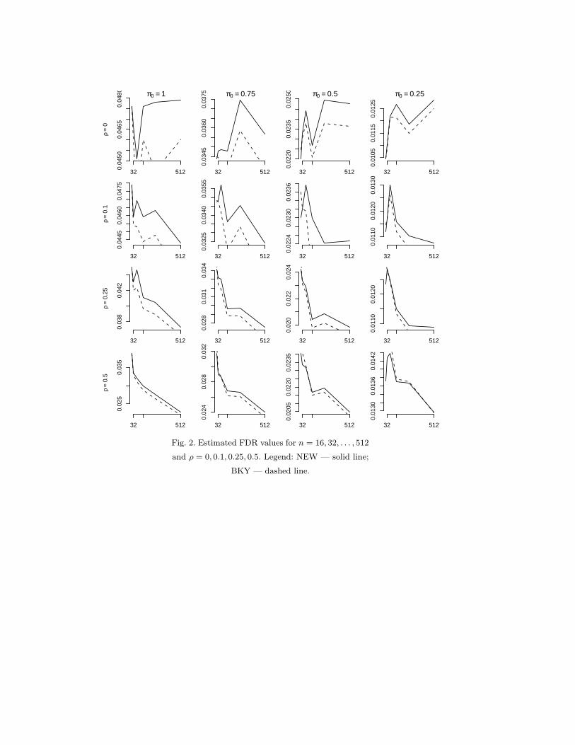
Figure 2 compares the FDR control and Table 2 lists the ratios of power of both

methods to the ‘Oracle’ method when n = 32, 128 and 512. The ‘Oracle’ method is the

BH method based on the critical values αi = iα/n0, which controls the FDR at the exact

level α under the independence of the test statistics. Obviously, it is not implementable

in practice as n0 is unknown, but it serves as a benchmark against which other methods

can be compared. As seen in Figure 2, our proposed method, which is known to control

the FDR at the desired level α = 0.05 under independence, can continue to maintain a

control over the FDR even under positive dependence, like the BKY method, although

ours is often less conservative. Also in terms of power, as seen from Table 2, our method

appears to be more powerful than the BKY method in most of the cases considered,

especially when the correlation is not very high.

The second part of the study was conducted by setting n = 5000. The simulated FDR

and power were also based on 10,000 iterations. The comparison between simulated FDR

of the two methods is presented in Figure 3. Again, there is evidence that our method

can continue to control the FDR under positive dependence, at least when the p-values

are equally correlated. The power comparisons in this case are displayed in Figures 4 and

5. Figure 4 indicates that the proposed method is more powerful than the BKY when the

16

Table 2. Estimated power for n = 32, 128, 512 and ρ = 0, 0.1, 0.25, 0.5

π0 = 0.25 π0 = 0.5 π0 = 0.75

n 32 128 512 32 128 512 32 128 512

ρ = 0 new/oracle 0.1881 0.1160 0.0737 0.4661 0.3935 0.3111 0.7553 0.7188 0.7088

BKY/oracle 0.1867 0.1105 0.0682 0.4618 0.3746 0.2925 0.7460 0.6914 0.6692

ρ = 0.1 new/oracle 0.2281 0.1769 0.1479 0.4956 0.4142 0.3550 0.7868 0.7060 0.6408

BKY/oracle 0.2293 0.1714 0.1403 0.4937 0.3979 0.3354 0.7796 0.6794 0.6024

ρ = 0.25 new/oracle 0.2846 0.2530 0.2373 0.5291 0.4949 0.4582 0.7542 0.7502 0.6979

BKY/oracle 0.2908 0.2495 0.2305 0.5333 0.4829 0.4423 0.7467 0.7294 0.6650

ρ = 0.5 new/oracle 0.3618 0.3391 0.3288 0.5942 0.5729 0.5551 0.7808 0.7895 0.7618

BKY/oracle 0.3755 0.3438 0.3305 0.6096 0.5725 0.5478 0.7876 0.7781 0.7432

correlation between the test statistics is moderately low. Figure 5 compares the power

of the two methods under the condition of high proportion of true null, π0 ≥ 0.9, which

is often the case in modern multiple testing situations. The proposed method seems to

be more powerful then the BKY method in such situations.

In conclusion, the simulation study seems to indicate that the new proposed method

can control the FDR under positive dependence of the p-values. It is more powerful than

the BKY method under positive but not very high correlations between the test statistics.

When there is a large proportion of true null hypotheses, the new method appears to

perform better than the BKY method even in the case of high correlations.

6. An Application to Breast Cancer Data

We applied both the new adaptive BH and the BKY methods to the breast cancer data

of Hedenfalk et al. (2001) available at http://www.nejm.org/general/content/supplemen-

tal/hedenfalk/index.html; see also Storey and Tibshirani (2003) from http://genomine.

org/qvalue/results.html. The results are presented in this section.

The data consists of 3,226 genes on 7 BRCA1 arrays, 8 BRCA2 arrays and 7 sporadic

tumors. The goal of the study is to establish differences in gene expression patterns

between these tumor groups. Here we analyzed this data with permutation t-test to

compare BRCA1 and BRCA2. The data were entered into R and all analyses were done

using R. As Storey and Tibshirani (2003) did, if any gene had one or more measurement

17

(log2 expression value) exceeding 20, then this gene was eliminated. This left n = 3170

genes for permutation t-test.

We tested each gene for differential expression between BRCA1 and BRCA2 by using a

two-sample t-test. The p-values were calculated using a permutation method as in Storey

and Tibshirani (2003). We did B = 100 permutations for each gene and got a set of null

statistics t0b1 , . . . , t0b

n , b = 1, . . . , B. The p-value of the permutation t-test for gene i was

calculated by

pi =B∑

b=1

#{j : |t0bj | ≥ |ti|, j = 1, . . . , n}

nB

The new adaptive method identifies 94 significant genes at the 0.05 level of false discov-

ery rate, whereas, the BKY method gets 93 significant genes. This additional significant

gene picked up by our method is intercellular adhesion molecule 2 (clone 471918).

7. Concluding Remarks

Adaptive BH methods other than those reviewed here have been proposed in the

literature; see, for instance, Sarkar (2008b). Among these, the BKY method has received

much attention since there is numerical evidence that it can continue to control the FDR

under some form of positive dependence among the test statistics. The new adaptive BH

method we propose in this article competes well with the BKY method. Like the BKY

method, it controls the FDR with independent p-values and, as can be seen numerically,

continue to maintain the control with the same type of positively dependent p-values as

in the BKY method. More importantly, it can perform better than the BKY method

in some instances, especially when the proportion of true null hypotheses is very large,

which happens in many applications.

We have considered using λ = 0.5 in the STS procedure, since this is what Storey,

Taylor and Siegmund (2004) have suggested, even though it may not control the FDR

under positive dependence, and α/(1 + α) for γ in our procedure, since this is what

Benjamini, Krieger and Yekutieli (2006) have also considered for the q in their procedure.

All these procedures can be proven to control the FDR under independence if other

different values are chosen for λ, q and γ. But, the BKY as well as our procedures may

18

not continue to control the FDR under positive dependence with these other values of γ

and q.

Acknowledgement

The research is supported by NSF Grant DMS-0603868.

References

Benjamini, Y. & Hochberg, Y. (1995). Controlling the false discovery rate: a practical and powerful

approach to multiple testing. J. R. Stat. Soc. B. 57, 289–300.

Benjamini, Y. & Hochberg, Y. (2000). On the adaptive control of the false discovery rate in multiple

testing with independent statistics. Journal of educational and behavioral statistics 25, 60–83.

Benjamini, Y., Krieger, A. & Yekutieli, D. (2006). Adaptive linear step-up procedures that control

the false discovery rate. Biometrica 93, 491–507.

Benjamini, Y. & Yekutieli, D. (2001). The control of the false discovery rate in multiple testing under

dependency. Ann. Statist. 29, 1165–1188.

Broberg, P. (2005). A comparative review of estimates of the proportion unchanged genes and the false

discovery rate. BMC Bioinformatics 6, 199.

Finner, H., Dickhaus, T. & Roters, M. (2009). On the false discovery rate and an asymptotically

optimal rejection curve. Ann. Statist. 37, 596–618.

Finner, H. & Roters, M. (2001). On the false discovery rate and expected type I errors. Biometrical

Journal 43, 985–1005.

Gavrilov, Y., Benjamini, Y. & Sakar, S. K. (2009). An adaptive step-down procedure with proven

FDR control. Ann. Statist. 37(2), 619–629.

Hommel, G. (1988). A stepwise rejective multiple test procedure based on a modified Bonferroni test.

Biometrika 75, 383–386.

Langaas, M. & Lindqvist, B. H. (2005). Estimating the proportion of true null hypotheses, with

application to DNA microarray data. Journal of the Royal Statistical Society, Series B (Methodological)

67, 555–572.

Liu, F. & Sarkar, S. K. (2009). A note on estimating the false discovery rate under mixture model.

Journal of Statistical Planning and Inference. To appear

Lu, X. & Perkins, D. L. (2007). Re-sampling strategy to improve the estimation of number of null

hypotheses in FDR control under strong correlation structures. BMC Bioinformatics 8, 157.

Pounds, S. & Morris, S. W. (2003). Estimating the occurrence of false positives and false nega-

tives in microarray studies by approximating and partitioning the empirical distribution of p-values.

Bioinformatics 19(10), 1236–1242.

Pounds, S. & Cheng, C. (2004). Improving false discovery rate estimation. Bioinformatics 20(11),

1737–1745.

Romano, J. P., Shaikh, A. M. & Wolf, M. (2008). Control of the false discovery rate under dependence

19

using the bootstrap and subsampling. TEST 17, 417–442.

Sarkar, S. K. (1998). Some probability inequalities for ordered MTP2 random variables: a proof of the

simes conjecture. Annals of Statistics 26(2), 494–504.

Sarkar, S. K. (2002). Some results on false discovery rate in stepwise multiple testing procedures.

Annals of Statistics 30, 239–257.

Sarkar, S. K. (2004). FDR-controlling procedures and their false negatives rates. Journal of Statistical

Planning and Inference 125, 119–139.

Sarkar, S. K. (2006). False discovery and false non-discovery rates in single-step multiple testing

procedures. Annals of Statistics 34, 394–415.

Sarkar, S. K. (2007). Stepup procedures controlling generalized FWER and generalized FDR. Annals

of Statistics 35, 2405–2420.

Sarkar, S. K. (2008a). On the Simes inequality and its generalization. IMS Collections Beyond Para-

metrics in Interdisciplinary Research: Festschrift in Honor of Professor Pranab K. Sen 1, 231–242.

Sarkar, S. K. (2008b). On methods controlling the False Discovery Rate (with discussions). Sankhya

70, 135–168.

Sarkar, S. K. & Chang, C.-K. (1997). The simes method for multiple hypothesis testing with positively

dependent test statistics. Journal of the American Statistical Association 92, 1601–1608.

Schweder, R. & Spjotvoll, E. (1982). Plots of p-values to evaluate many tests simultaneously.

Biometrika 69, 493–502.

Simes, R. J. (1986). An improved Bonferroni procedure for multiple tests of significance. Biometrika

73, 751–754.

Storey, J. D. (2002). A direct approach to false discovery rates. Journal of the Royal Statistical Society,

Series B 64, 479–498.

Storey, J. D. (2003). The positive false discovery rate: a bayesian interpretation and the q-value.

Annals of Statistics 31, 2013–2035.

Storey, J. D., Taylor, J.E. & Siegmund, D. (2004). Strong control, conservative point estimation,

and simultaneous conservative consistency of false discovery rates: A unified approach. J. Roy. Statist.

Soc. B 66, 187–205.

Storey, J. D. & Tibshirani, R. (2003). Statistical Significance for genome-wide studies. Proc. Nat.

Acad. Sci 100, 9440–9445.

20

NEW BKY STS NEW BKY STS NEW BKY STS NEW BKY STS

020

0040

0060

0080

0010

000

&(n = 5000, π 0 = 0.5)

Correlation is 0 Correlation is 0.25 Correlation is 0.5 Correlation is 0.75

n 0

Fig. 1. The simulated distribution of n̂NEW0 , n̂STS

0

and n̂BKY0 for the cases of n = 5000, n0 = 2500 and

ρ = 0, 0.25, 0.5 and 0.75. Each box displays the me-

dian and quartiles as usual. The whiskers extend to

the 5th and 95th percentiles. The circles are the ex-

treme values, i.e. the 0.01th and 99.99th percentiles.

21

π0 = 1ρ

=0

32 512

0.04

500.

0465

0.04

80 π0 = 0.75

32 512

0.03

450.

0360

0.03

75 π0 = 0.5

32 512

0.02

200.

0235

0.02

50 π0 = 0.25

32 512

0.01

050.

0115

0.01

25

ρ=

0.1

32 512

0.04

450.

0460

0.04

75

32 512

0.03

250.

0340

0.03

55

32 512

0.02

240.

0230

0.02

36

32 512

0.01

100.

0120

0.01

30

ρ=

0.25

32 512

0.03

80.

042

32 512

0.02

80.

031

0.03

4

32 512

0.02

00.

022

0.02

4

32 512

0.01

100.

0120

ρ=

0.5

32 512

0.02

50.

035

32 512

0.02

40.

028

0.03

2

32 512

0.02

050.

0220

0.02

35

32 512

0.01

300.

0136

0.01

42

Fig. 2. Estimated FDR values for n = 16, 32, . . . , 512

and ρ = 0, 0.1, 0.25, 0.5. Legend: NEW — solid line;

BKY — dashed line.

22

ρ = 0

n0

FD

R

0.00

0.01

0.02

0.03

0.04

0.05

0 1000 2000 3000 4000 5000

ρ = 0.1

n0

0.00

0.01

0.02

0.03

0.04

0 1000 2000 3000 4000 5000

ρ = 0.25

n0

FD

R

0.00

0.01

0.02

0.03

0 1000 2000 3000 4000 5000

ρ = 0.5

n0

0.000

0.005

0.010

0.015

0.020

0.025

0 1000 2000 3000 4000 5000

Fig. 3. Estimated FDR values for n = 5000 and ρ =

0, 0.1, 0.25, 0.5. Legend: NEW — solid line; BKY —

dashed line.

23

ρ = 0

n0

PO

WE

R

0.005

0.010

0.015

0 1000 2000 3000 4000

ρ = 0.1

n0

0.00

0.01

0.02

0.03

0.04

0 1000 2000 3000 4000

ρ = 0.25

n0

PO

WE

R

0.02

0.04

0.06

0.08

0 1000 2000 3000 4000

ρ = 0.5

n0

0.02

0.04

0.06

0.08

0.10

0.12

0 1000 2000 3000 4000

Fig. 4. Estimated power for n = 5000 and ρ =

0, 0.1, 0.25, 0.5. Legend: NEW — solid line; BKY —

dashed line.

24

ρ = 0

n0

pow

er

0.00065

0.00070

0.00075

0.00080

0.00085

4500 4600 4700 4800 4900

ρ = 0.1

n0

0.00100.00120.00140.00160.00180.0020

4500 4600 4700 4800 4900

ρ = 0.25

n0

pow

er

0.004

0.005

0.006

0.007

4500 4600 4700 4800 4900

ρ = 0.5

n0

0.010

0.012

0.014

0.016

0.018

4500 4600 4700 4800 4900

ρ = 0.7

n0

pow

er

0.0140.0160.0180.0200.0220.024

4500 4600 4700 4800 4900

ρ = 0.9

n0

0.018

0.020

0.022

0.024

0.026

4500 4600 4700 4800 4900

Fig. 5. Estimated power for n = 5000, π0 =

0.9, 0.92, 0.94, 0.96, 0.98 and ρ = 0, 0.1, 0.25, 0.5, 0.75

and 0.9. Legend: NEW — solid line; BKY — dashed

line.

25