a net zero greenhouse gas feasibility study for green
TRANSCRIPT

James Madison UniversityJMU Scholarly Commons
Senior Honors Projects, 2010-current Honors College
Spring 2015
A net zero greenhouse gas feasibility study forGreen Fence FarmAshleigh CottingJames Madison University
Follow this and additional works at: https://commons.lib.jmu.edu/honors201019Part of the Sustainability Commons
This Thesis is brought to you for free and open access by the Honors College at JMU Scholarly Commons. It has been accepted for inclusion in SeniorHonors Projects, 2010-current by an authorized administrator of JMU Scholarly Commons. For more information, please [email protected].
Recommended CitationCotting, Ashleigh, "A net zero greenhouse gas feasibility study for Green Fence Farm" (2015). Senior Honors Projects, 2010-current. 28.https://commons.lib.jmu.edu/honors201019/28
A Net Zero Greenhouse Gas Emissions Feasibility Study for Green Fence Farm
_______________________
An Honors Program Project Presented to
the Faculty of the Undergraduate
College of Integrated Science and Engineering
James Madison University
_______________________
In Partial Fulfillment of the Requirements
For the Degree of Bachelor of Sciences
by Ashleigh Marie Cotting
May 2015
Accepted by the faculty of the Department of Integrated Science and Technology, James Madison University, in
partial fulfillment of the requirements for the Honors Program.
FACULTY COMMITTEE:
Project Advisor: Paul Goodall, M.B.A.
Associate Professor, Integrated Science and
Technology
Reader: Jonathan Miles, Ph.D.
Professor, Director of the Center for Wind Energy
Reader: Blaine Loos
Energy Project Analyst, Center for Wind Energy
PUBLIC PRESENTATION
This work is accepted for presentation, in part or in full, at ISAT Senior Symposium on 4/17/15.

1
Table of Contents
Acknowledgements ....................................................................................................................................... 4
Abstract ......................................................................................................................................................... 5
Introduction and Background ....................................................................................................................... 6
Climate Change as a Global Issue............................................................................................................. 6
Agriculture: A Growing Greenhouse Gas Contributor ............................................................................. 7
Stakeholder Analysis ................................................................................................................................ 9
A More Conscious Consumer ............................................................................................................... 9
Increase in Organic Farms .................................................................................................................. 10
Benefits to Communities around Farms .............................................................................................. 11
Project Description ...................................................................................................................................... 13
Project Statement .................................................................................................................................... 13
Introduction to Green Fence Farm .......................................................................................................... 13
Farming Operations ............................................................................................................................ 13
Project Purpose ................................................................................................................................... 15
Methodology ............................................................................................................................................... 16
Farm System Analysis ............................................................................................................................ 16
Determining Current Greenhouse Gas Emissions................................................................................... 16
On Farm Fuel Usage ........................................................................................................................... 16
Greenhouse Gas Inventory .................................................................................................................. 17
Determining Current Carbon Sequestration Capabilities ........................................................................ 17
Sequestration Capabilities of Soil ....................................................................................................... 17
Sequestration Capabilities of Trees ..................................................................................................... 17
Examining Ways to Reach Net Zero Greenhouse Gas Emissions .......................................................... 19
Lowering Carbon Dioxide Emissions ................................................................................................. 19
Increasing Sequestration Capabilities ................................................................................................. 25
Results and Analysis ................................................................................................................................... 27
Farm System Analysis ............................................................................................................................ 27
Current Greenhouse Gas Emissions ........................................................................................................ 27
On Farm Fuel Usage ........................................................................................................................... 27
Greenhouse Gas Inventory .................................................................................................................. 29
Current Carbon Sequestration Capabilities ............................................................................................. 31
Soil Sequestration ............................................................................................................................... 31
Tree Sequestration .............................................................................................................................. 32

2
Ways to Reach Net Zero Greenhouse Gas Emissions ............................................................................ 32
Lowering Carbon Dioxide Emissions ................................................................................................. 33
Increasing Sequestration Capabilities ................................................................................................. 43
Purchasing Carbon Offsets.................................................................................................................. 44
Recommendations ....................................................................................................................................... 45
Conclusions ................................................................................................................................................. 46

3
Table of Figures
Figure 1. Global Greenhouse Emissions by Gas, 1990-2010 (EPA, 2011). ................................... 6 Figure 2. Global Greenhouse Gas Emissions by Source. (EPA, 2013) .......................................... 8 Figure 3. EPA Emissions from Agriculture (Tg CO2 Eq.) ............................................................. 8 Figure 4. U.S. Organic Food Sales by Category. (USDA 2014) .................................................. 10 Figure 5. How Organic and Conventional Farming Compare Side by Side over 30 Years. (Rodale
Institute, 2014). ............................................................................................................................. 12 Figure 6. Evenly Spaced Sampling Grid for Tree Circumference Sampling. .............................. 18 Figure 7. Pinpointed Sampling Locations for Tree Circumference Sampling.............................. 18 Figure 8. The Energy Management Pyramid. (DOE, 2007). ........................................................ 20 Figure 9. Google SketchUp Rendering of the Green Fence Farm Workhouse. ........................... 20 Figure 10. Solar Pathfinder Kit (Solar Pathfinder, 2015) ............................................................. 21 Figure 11. Annual Energy Consumption Patterns for Green Fence Farm. ................................... 29 Figure 12. Roof Mount Solar PV System Rendering. .................................................................. 35 Figure 13. Ground Mount Solar PV System Rendering. .............................................................. 37 Figure 14. Graph of the Weibull Distribution for an 80m and a 20m Hub Height. ...................... 41
List of Tables
Table 1. Property Breakdown of Green Fence Farm. ................................................................... 13 Table 2. Animal Head Count for Summer 2014. .......................................................................... 13 Table 3. Representative Year of Fuel Consumption for Green Fence Farm. ............................... 28 Table 4. Carbon Dioxide Emissions from On Site Fuel Consumption. ........................................ 29 Table 5. Greenhouse Gas Inventory Results. ................................................................................ 29 Table 6. Sample of Data for Carbon Dioxide Stored by Trees on Site. ........................................ 32 Table 7. Current State of Greenhouse Gas Emissions and Sequestration for Green Fence Farm. 32 Table 8. Estimated Electricity Generation for a Roof Mount Solar PV System........................... 35 Table 9. Roof Mount Solar PV System Purchase and Installation Costs. .................................... 36 Table 10. Estimated Electricity Generation for a Ground Mount Solar PV System. ................... 38 Table 11. Ground Mount Solar PV System Purchase and Installation Costs. .............................. 38 Table 12. Average Wind Speeds and Weibull Constants from ArcMap. ..................................... 39 Table 13. Weibull Distribution for an 80m Hub Height. .............................................................. 39 Table 14. Estimated Weibull Distribution for a 20m Hub Height. ............................................... 40 Table 15. Annual Energy Output Estimates for a Bergey Excel 10k on Green Fence Farm. ....... 41 Table 16. Additional Cost to Purchase Electricity from Renewable Energy Projects. ................. 43 Table 17. Recommended Steps for Green Fence Farm to Reach Net Zero Greenhouse Gas
Emissions. ..................................................................................................................................... 45

4
Acknowledgements I would like to acknowledge all of the individuals who made this project possible:
My advisor, Professor Paul Goodall, for guiding me throughout the project.
Katherine Sparks and Nick Auclair for allowing me to use their farm as my project site.
Professors who helped me develop this project idea and complete it:
Dr. Maria Papadakis, JMU
Dr. Zachary Bortolot, JMU
Dr. Wayne Teel, JMU
Everyone who provided me with support during the completion of this project:
My family
Blaine Loos
All of my ISAT classmates.

5
Abstract The purpose of this project is to assess the ability of Green Fence Farm, a 17 acre sustainable
farming operation located in Greenville, VA, to become a net zero greenhouse gas farm
operation. This project was conducted in several phases. First, the types and quantities of
emissions were determined through an onsite fuel consumption evaluation and a greenhouse gas
inventory of farm operations. Next, and calculations were used to determine the carbon
sequestration capabilities of the soil and trees on the farm. Finally, ways to reduce emission and
increase sequestration were examined with the intent of reaching net zero greenhouse gas
emissions.
All of this information was used to develop a comprehensive plan for how Green Fence Farms
can reach net zero greenhouse gas emissions through changes in farming practices, energy
conservation and efficiency measures, fuel switching, and increasing carbon sequestration. The
plan includes suggested steps to take, as well as economic analyses for each recommendation.
This project is of global significance because agriculture is one of the world’s leading sources of
annual greenhouse gas emissions. Meeting the food and fiber needs of the world’s growing
population will require the agricultural sector to grow. However, given that the effects of global
climate change continues to worsen, it is imperative that while the agricultural sector grows, its
emissions do not. Reducing the greenhouse gas emissions of small farming operations is one way
to lessen the global impact of the agricultural sector.

6
Introduction and Background
Climate Change as a Global Issue The evidence in favor of rapid climate change is overwhelming. Global sea levels have risen 6.7 inches in
the last century. The 10 hottest years on the planet have all occur within the past 12 years. Oceans have
warmed 0.302°F since 1969 and ice sheets in Greenland and Antarctica are rapidly losing mass. Glaciers
around the world are retreating, the oceans have become 30% more acidic since the Industrial Revolution,
and snow cover across the Northern Hemisphere is decreasing. 97% of climate scientists agree that these
changes are very likely caused by human activities that produce greenhouse gases1.
According to the Environmental Protection Agency (EPA), net worldwide greenhouse gas emissions
increased 35% between 1990 and 2010. Error! Reference source not found. shows the worldwide
emissions of the main greenhouse gases, including carbon dioxide, methane, and nitrous oxide. Carbon
dioxide emissions have increased 42%, methane by 15%, and nitrous oxide by 9%.
These increasing emissions have global ramifications. In 2014, the Intergovernmental Panel on Climate
Change (IPCC) published “Climate Change 2014: Impacts, Adaptation, and Vulnerability2.” This
document begins by outlining the impacts of climate change on natural systems. Shrinking glaciers have
had adverse effects on downstream water resources, disrupting the fresh water supply for regions around
the world. The localized effects of climate change have caused terrestrial, freshwater, and marine species
to shift their geographic ranges, seasonal activities migration patterns, and species interactions, all of
1 http://climate.nasa.gov/evidence/ 2 http://www.ipcc.ch/pdf/assessment-report/ar5/wg2/ar5_wgII_spm_en.pdf
Figure 1. Global Greenhouse Emissions by Gas, 1990-2010 (EPA, 2011).

7
which can affect human food supply. The increase in climate extremes has had negative effects on crop
yields, disturbing food production and reducing the food security of many nations. Extreme weather
events such as hurricanes, flooding, and forest fires have caused damage to infrastructure and settlements
in countries at all levels of development2.
The effects of climate change aggravate other issues within countries both directly and indirectly. For
instance, when food production is interrupted, the farmer is directly affected because he now may not be
able to feed his family. His crop failure indirectly affects global food prices, meaning he may not be able
to make a profit that year. These direct and indirect effects are felt by people in all countries; no level of
development is immune2.
Climate change has caused a reduction in significant reduction in essential resources for some regions of
the world. If these situations cannot be reversed, violent conflicts are going to break out in resource scare
areas. Countries will fight for food, water, and energy resources. The current imminence of these conflicts
threatens the safety of people worldwide.
Clearly, climate change has far reaching, long term effects. That being said, they are not unpreventable.
The good news about the anthropogenic nature of climate change is that humans can change their
behavior and reduce their impact. People have the ability to affect positive change by reducing
greenhouse gas emitting activities.
Agriculture: A Growing Greenhouse Gas Contributor The issue of climate change can be overwhelming at first; its consequences alter incredibly complex
systems. One effective strategy for approaching such a complicated problem is by breaking it down into
smaller parts. For instance, global emissions can be broken down by the economic activities that lead to
their emission. This breakdown is shown in Figure 2. By focusing on one sector at a time, it is
possible to determine ways to reduce greenhouse gas emitting activities.

8
As the above chart shows, agricultural activities account for 9% of global greenhouse gas emissions3.
Since 1990, greenhouse gas emissions have increased 19%4. The sector is worth examining because it is
associated with all three of the most problematic greenhouse gases: methane, nitrous oxide, and carbon
dioxide. Methane and nitrous oxide emissions come directly from agricultural practices such as manure
and land management, crop cultivation, and burning of agriculture residues5. Figure 3 shows estimates for
methane and nitrous oxide emissions from US agriculture activity from 1990-2012.
As Figure 3 shows, there are many aspects of agricultural practices that have the potential to be altered to
reduce methane and nitrous oxide emissions.
Carbon dioxide emissions from agriculture result mainly from on-farm energy use. The agricultural sector
also plays a crucial role in carbon fluxes. When land is converted for agricultural use, it can release
carbon dioxide and reduce an area’s sequestration capabilities. In 2007, proper forest management
resulted in an offset of 14.9% of US greenhouse gas emissions6. Farms are provide an opportunity to
implement land and forest management practices that optimize carbon sequestration.
The future of the sector is certain; people will always need food, so agricultural activities will continue
on. In fact, the U.N. Population Division estimates that by mid-century, the world population will be at
9.2 billion7, suggesting that the sector will have to continue to grow. In light of the rapidly changing
climate, it is crucial for the world’s health that as the agriculture sector grows, its emissions do not.
Fortunately, there are many opportunities to reduce agricultural emissions, and people have begun to take
an interest in doing so.
3 http://epa.gov/climatechange/ghgemissions/sources/agriculture.html 4 http://epa.gov/climatechange/ghgemissions/sources/agriculture.html 5 http://www.epa.gov/climatechange/Downloads/ghgemissions/US-GHG-Inventory-2014-Chapter-6-Agriculture.pdf 6 http://unfccc.int/resource/docs/natc/usa_nc5.pdf 7 http://www.worldwatch.org/node/6038
Figure 2. Global Greenhouse Gas Emissions by Source. (EPA, 2013)
Figure 3. EPA Emissions from Agriculture (Tg CO2 Eq.)
9
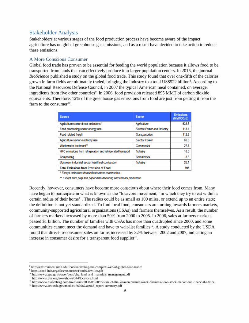
Stakeholder Analysis Stakeholders at various stages of the food production process have become aware of the impact
agriculture has on global greenhouse gas emissions, and as a result have decided to take action to reduce
these emissions.
A More Conscious Consumer
Global food trade has proven to be essential for feeding the world population because it allows food to be
transported from lands that can effectively produce it to larger population centers. In 2015, the journal
BioScience published a study on the global food trade. This study found that over one-fifth of the calories
grown in farm fields are ultimately traded, bringing the industry to a total US$522 billion8. According to
the National Resources Defense Council, in 2007 the typical American meal contained, on average,
ingredients from five other countries9. In 2006, food provision released 895 MMT of carbon dioxide
equivalents. Therefore, 12% of the greenhouse gas emissions from food are just from getting it from the
farm to the consumer10.
Recently, however, consumers have become more conscious about where their food comes from. Many
have begun to participate in what is known as the “locavore movement,” in which they try to eat within a
certain radius of their home11. The radius could be as small as 100 miles, or extend up to an entire state;
the definition is not yet standardized. To find local food, consumers are turning towards farmers markets,
community-supported agricultural organizations (CSAs) and farmers themselves. As a result, the number
of farmers markets increased by more than 50% from 2000 to 2005. In 2006, sales at farmers markets
passed $1 billion. The number of families with CSAs has more than quadrupled since 2000, and some
communities cannot meet the demand and have to wait-list families12. A study conducted by the USDA
found that direct-to-consumer sales on farms increased by 32% between 2002 and 2007, indicating an
increase in consumer desire for a transparent food supplier13.
8 http://environment.umn.edu/food/unraveling-the-complex-web-of-global-food-trade/ 9 https://food-hub.org/files/resources/Food%20Miles.pdf 10 http://www.epa.gov/oswer/docs/ghg_land_and_materials_management.pdf 11 http://www.pbs.org/now/shows/344/locavore.html 12 http://www.bloomberg.com/bw/stories/2008-05-20/the-rise-of-the-locavorebusinessweek-business-news-stock-market-and-financial-advice 13 http://www.ers.usda.gov/media/1763062/ap068_report-summary.pdf
10
In 2011, the Food Marketing Institute conducted a survey to determine why consumers were participating
in the locavore movement. Another survey found that 27% of participants chose to buy local because due
to concerns over the environmental impacts of food transportationError! Bookmark not defined..
The same survey found that 83% of those surveyed said they buy local food because it is fresher, while
56% said they prefer the taste. This suggests that consumers are also beginning to pay attention to who
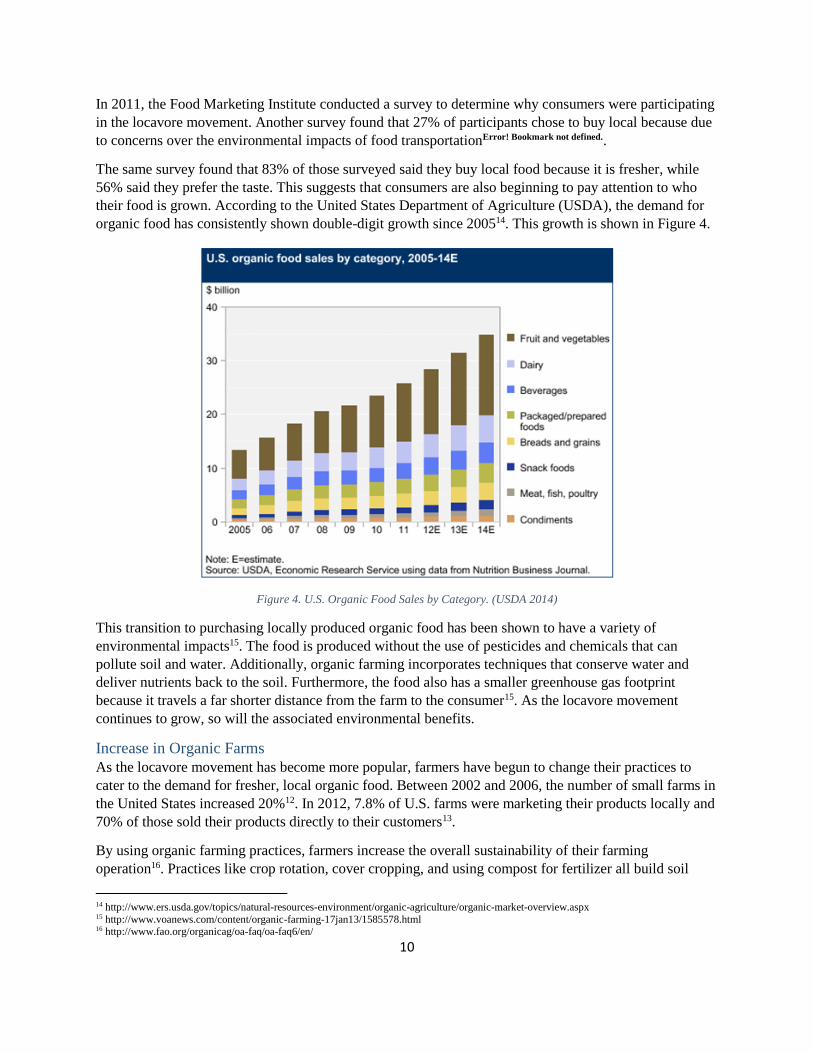
their food is grown. According to the United States Department of Agriculture (USDA), the demand for
organic food has consistently shown double-digit growth since 200514. This growth is shown in Figure 4.
Figure 4. U.S. Organic Food Sales by Category. (USDA 2014)
This transition to purchasing locally produced organic food has been shown to have a variety of
environmental impacts15. The food is produced without the use of pesticides and chemicals that can
pollute soil and water. Additionally, organic farming incorporates techniques that conserve water and
deliver nutrients back to the soil. Furthermore, the food also has a smaller greenhouse gas footprint
because it travels a far shorter distance from the farm to the consumer15. As the locavore movement
continues to grow, so will the associated environmental benefits.
Increase in Organic Farms
As the locavore movement has become more popular, farmers have begun to change their practices to
cater to the demand for fresher, local organic food. Between 2002 and 2006, the number of small farms in
the United States increased 20%12. In 2012, 7.8% of U.S. farms were marketing their products locally and
70% of those sold their products directly to their customers13.
By using organic farming practices, farmers increase the overall sustainability of their farming
operation16. Practices like crop rotation, cover cropping, and using compost for fertilizer all build soil
14 http://www.ers.usda.gov/topics/natural-resources-environment/organic-agriculture/organic-market-overview.aspx 15 http://www.voanews.com/content/organic-farming-17jan13/1585578.html 16 http://www.fao.org/organicag/oa-faq/oa-faq6/en/
11
health by returning nutrients to the soil. The water used on site is not polluted by pesticide runoff.
Varying the crops grown through practices like symbiotic cropping increases the biodiversity of the farm,
which can optimize nutrient and energy cycling on the farm16.
Producing and selling organic produce locally also has economic benefits for the farmer. Organic farming
can have lower production costs because it does not require pesticides or the intensive land management
techniques that conventional farming does17. Additionally, farmers selling organic products to local
customers can do so at a premium price. As a result, organic farming is economically feasible and, in the
right context, can be more lucrative than conventional farming17.
The number of farmers running organic operations and selling their products locally has been increasing
to the point that it has influenced policy. When the Farm Bill was updated in 2008, $2.3 billion was set
aside for specialty crops that are typically produced by smaller farms instead of big agribusinesses.
Additionally, the bill allowed farms to get up to 75% of their organic certification costs reimbursed12. As
the small, organic farming industry grows, similar policy changes are bound to occur, making the
business even better for farmers.
Benefits to Communities around Farms
The communities around farms that sell their organic produce locally see benefits as well. A study
conducted by the Union of Concerned Scientists found that expanding local food systems can improve the
local economy. Farmers markets, for instance, create jobs and ensure that a greater percentage of the sales
revenue is retained locally. Furthermore, farmers who sell locally are connected to their communities and
are therefore likely to purchase their equipment and raw materials from local suppliers. This can increase
labor and household incomes, which in turn encourages community residents to spend more,
strengthening the economy further18.
Having access to locally grown organic food is also beneficial for the health of a community. For
instance, the Farm to School program has vastly improved student health by providing them with access
to healthier food options in the cafeteria19. Children who attend a school with the Farm to School program
receive on average 0.99-1.3 additional servings of fruits and vegetables each day. Furthermore, the
program teaches children about agriculture, the environment, and the relationship between the two. The
children are then able to bring this knowledge home to their families, which encourages them to shop
locally and purchase healthy foods. This increased awareness of eating healthy tends to translate into an
interest in how to be healthy in other ways, such as increased physical activity. Without a farm in the area
to supply the Farm to School program, communities would not see these health and education benefits19.
Farms that operate organically and sell their produce locally release far less greenhouse gases than large
agribusinesses do, offering benefits to the national, local, and global communities. By shortening the
distance food travels from the farm to a consumer, farmers can lower the greenhouse gas emission
associated with food transportation. Organic practices like no-till, returning crop residue to soil, and cover
cropping help sequester carbon on site. According to a study conducted by Rodale Institute, if all cropland
were converted to organic farmland, the land could sequester up to 40% of annual carbon dioxide
emissions. The same study found that and organic farm with the same yield as a conventional farm has a
17 http://www.sciencedaily.com/releases/2011/09/110901093715.htm 18 http://www.ucsusa.org/sites/default/files/legacy/assets/documents/food_and_agriculture/market-forces-exec-summary.pdf 19 http://www.farmtoschool.org/Resources/BenefitsFactSheet.pdf
12
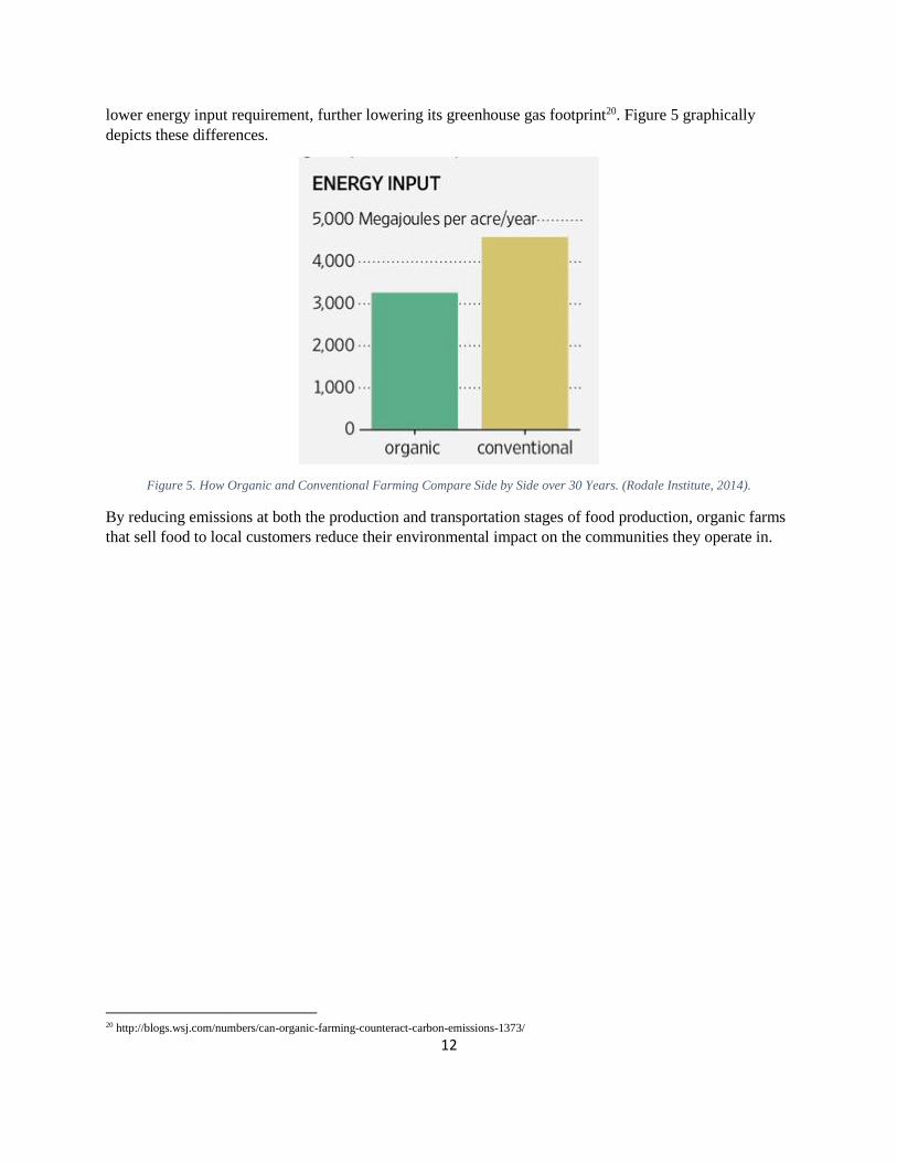
lower energy input requirement, further lowering its greenhouse gas footprint20. Figure 5 graphically
depicts these differences.
Figure 5. How Organic and Conventional Farming Compare Side by Side over 30 Years. (Rodale Institute, 2014).
By reducing emissions at both the production and transportation stages of food production, organic farms
that sell food to local customers reduce their environmental impact on the communities they operate in.
20 http://blogs.wsj.com/numbers/can-organic-farming-counteract-carbon-emissions-1373/
13
Project Description
Project Statement As consumers move towards purchasing from local organic farms, it becomes more important to ensure
that these farms do in fact operate in an environmentally friend, sustainable manner. Purchasing locally
grown organic food only yields environmental benefits when the farm is operating efficiently. One way to
maximize the environmental sustainability of a farm is to make it a net zero greenhouse operation. This
project serves as a case study to determine what steps can be taken to get a small organic farming
operation to net zero.
Introduction to Green Fence Farm Green Fence Farm is a 17 acre multi-product sustainably run farming operation owned by Katherine
Sparks and Nick Auclair. The farm is located in Greenville, Virginia which is approximately 40 minutes
south of Harrisonburg, Virginia.
Farming Operations
Sparks and Auclair use their land to grow crops and raise animals. The land on the farm is divided up into
three different use categories, which can be seen in Table 1.
Table 1. Property Breakdown of Green Fence Farm.
Percentage Acres Hectares
Forested 59% 10.00 4.05
Grassland 35% 6.00 2.43
Cropland 6% 1.00 0.40
Green Fence Farm used to be a Christmas tree farm and is today still heavily forested with loblolly pine
trees. This area, combined with the grassland, serves as grazing areas for the animals on site. Table 2
provides the animal head count for summer 2014.
Table 2. Animal Head Count for Summer 2014.
Dairy Cows 0
Other Cattle 0
Buffalo 0
Sheep 10
Goats 0
Camels 0
Horses 0
Mules and Asses 0
Swine 5
Poultry 75
Other2
50
Animal Head Count
Every spring, Sparks and Auclair purchase piglets, lambs, and turkeys to raise throughout the summer. In
the fall, the turkeys are slaughtered on site and sold to individual customers. The pigs and sheep are sold
14
to local restaurants. The pigs reside in a pen that is mainly in the forested area of the property. The sheep
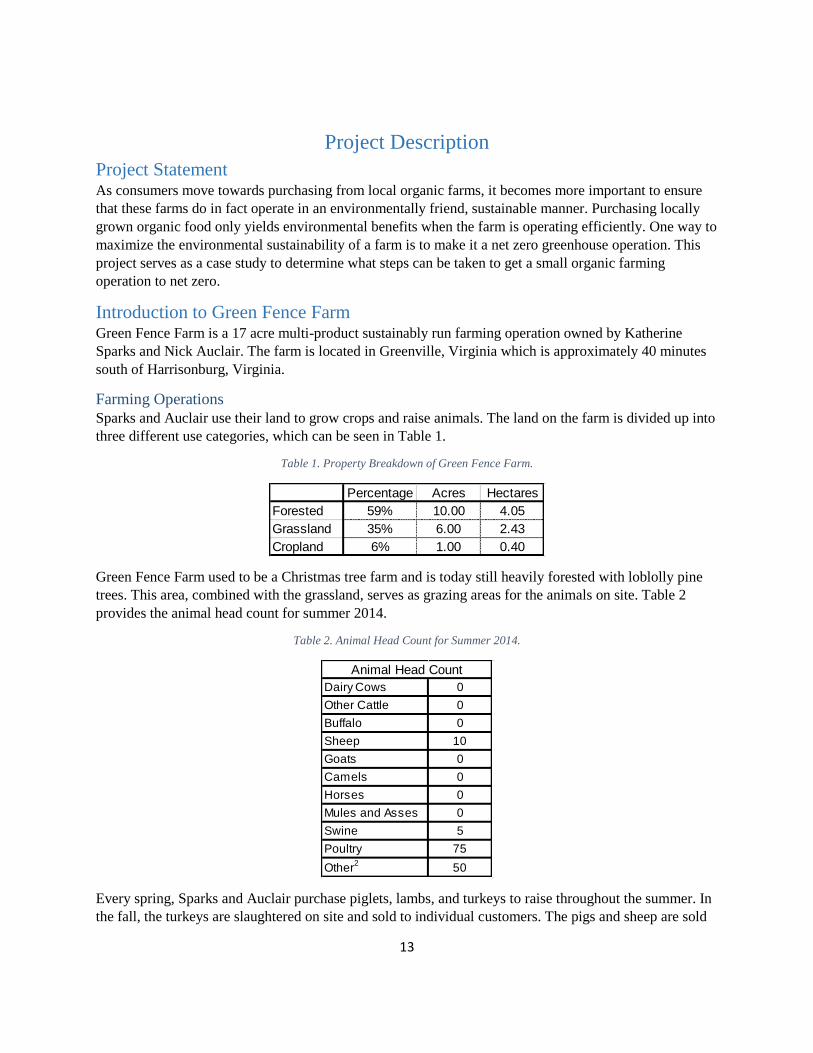
are allow free range of the grassland and forest. The turkeys graze rotationally and live in houses than can
be moved by hand. An example of the turkey houses can be seen in Image 1.
Image 1. Turkey House Designed for Rotational Grazing.
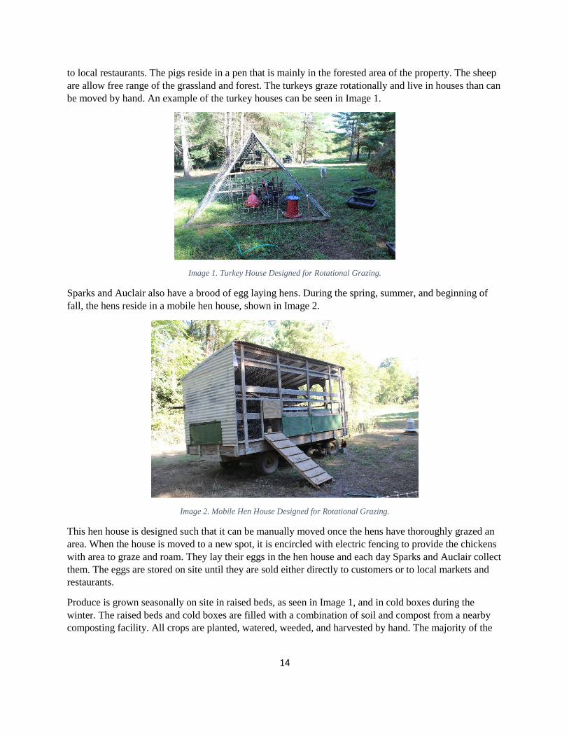
Sparks and Auclair also have a brood of egg laying hens. During the spring, summer, and beginning of
fall, the hens reside in a mobile hen house, shown in Image 2.
Image 2. Mobile Hen House Designed for Rotational Grazing.
This hen house is designed such that it can be manually moved once the hens have thoroughly grazed an
area. When the house is moved to a new spot, it is encircled with electric fencing to provide the chickens
with area to graze and roam. They lay their eggs in the hen house and each day Sparks and Auclair collect
them. The eggs are stored on site until they are sold either directly to customers or to local markets and
restaurants.
Produce is grown seasonally on site in raised beds, as seen in Image 1, and in cold boxes during the
winter. The raised beds and cold boxes are filled with a combination of soil and compost from a nearby
composting facility. All crops are planted, watered, weeded, and harvested by hand. The majority of the

15
produce grown at Green Fence Farm is consumed by Sparks, Auclair, and their family. Excess produce is
stored on site in freezers for later use.
Image 3. Raised Beds Used to Grow Crops.
Other features of Green Fence Farm include a fungi garden, a hand planted meadow, a passive rainwater
collection system, and a bee keeping facility. Sparks and Auclair have a home on the farm, but its energy
usage and associated emissions were excluded from this analysis.
Project Purpose
The purpose of this project is to assess the ability of Green Fence Farm, a 17 acre sustainable farming
operation located in Greenville, VA, to become a net zero greenhouse gas farm operation. Despite all of
the sustainable practices being implemented at Green Fence Farm, there are many opportunities
for improvement. A significant contribution that agricultural systems can make to the
environment is through reduced greenhouse gas emissions. Helping Green Fence Farm assess
their ability to get to net zero greenhouse gas emissions would be a major step in achieving
overall sustainability. Furthermore, the model developed for Green Fence Farm can serve as a
best practices guide for other small sustainable farms in the area.

16
Methodology In order for Green Fence Farm to be a net zero greenhouse gas farming operation, its greenhouse gas
emissions must be equal to its on-site greenhouse gas storage capabilities.
This project was completed in four phases. First, several site visits were made to learn about the farm and
its associated activities. Next, the current levels of greenhouse gas emissions were determined. Then, a
carbon sequestration analysis was performed to determine how much carbon is currently stored on site in
carbon sinks. Finally, methods for reaching net zero greenhouse gas emissions were researched. This
included a renewable energy assessment and research regarding how to increase carbon sequestration on
site.
Farm System Analysis This project began with a series of farm visits. These visits were used to catalogue information regarding
farming inputs, processes, and outputs. Photographs were taken in addition to written documentation.
This information was then used to create a series of systems diagrams that separated the components of
the farming system into appropriate categories. This process was used to draw the system boundary for
the analysis. Only the farming activities that occur on the farm itself were considered in this analysis.
Determining Current Greenhouse Gas Emissions During the second phase of this project, current greenhouse gas emissions were quantified. This was
accomplished through an analysis of on farm fuel usage, as well as a greenhouse gas inventory for farm
activities.
It should be noted that all greenhouse gas emissions are given in units of carbon dioxide equivalents. This
methodology was chosen because emission levels of methane and nitrogen dioxide were too low to
financially justify specific mitigation techniques.
On Farm Fuel Usage
The first step taken in determining Green Fence Farm’s current levels of greenhouse gas emissions was
examining utility bills. The farm has three energy systems: electricity, gas, and a backup propane
generator. Utility data from the past 18 months was collected and analyzed. This data was logged into an
Excel file. To create a representative year of fuel usage, months with two or more data points were
averaged together.
Once the representative year was created, the associated annual greenhouse gas emissions were
calculated. This was done using Emissions Factors for Greenhouse Gas Inventories provided by the
EPA21. Once the correct carbon dioxide factor was selected, Equation 1 was used to calculate the
emissions from Green Fence Farm’s energy usage.
Equation 1
Once the emissions for each fuel source were calculated, the total carbon dioxide emissions for on-site
energy usage was determined. This was calculated by adding all of the emissions from electricity, gas,
and propane together.
21 http://www.epa.gov/climateleadership/documents/emission-factors.pdf

17
Greenhouse Gas Inventory
The next step taken for this project was determining the amount of greenhouse gas emissions from
farming activities. This was conducted using the 2006 Intergovernmental Panel on Climate Change
(IPCC) Guidelines for Greenhouse Gas Inventories for Agriculture, Forestry, and Other Land Use22. This
inventory method was chosen over other options because it could be tailored to Green Fence Farm. The
document, which is broken down primarily by land use category, provides step by step guidance for
calculating the greenhouse gas emissions associated with individual agricultural and land management
activities. The first step in creating an inventory specific for Green Fence Farm was to determine which
sets of calculations were to be included based on the farming operation. Each activity selected had an
accompanying worksheet in the IPCC guidelines. These worksheets were downloaded and compiled into
one Excel workbook. The specific calculations each worksheet required were performed using data from
Green Fence farm (shown in Tables 1 and 2) and factors from the IPCC document which were based on
information such as location and soil type.
The IPCC greenhouse gas inventory calculations provided the greenhouse emissions associated with on
farm activities in terms of kilogram of methane, nitrogen dioxide, and carbon gains or losses. Due to the
nature of this analysis, values given for methane nitrogen dioxide emissions were converted into carbon
dioxide equivalents. This was done using Emissions Factors for Greenhouse Gas Inventories21.
The greenhouse gas emissions calculated through the greenhouse gas inventory were then combined with
the emissions calculated for on-site energy usage to determine total annual emissions for Green Fence
Farm.
Determining Current Carbon Sequestration Capabilities The goal of the third phase of this project was to calculate how much carbon is currently stored on site.
This was accomplished by analyzing the sequestration capabilities of the soil and the trees.
Sequestration Capabilities of Soil
The carbon gains and losses associated with the soil were calculated during the greenhouse gas inventory
that occurred during Phase I. The same methodology was used to determine how much carbon the soil
sequesters based on land use and management.
Sequestration Capabilities of Trees
The methodology for this part of the project was adapted from a Geographic Science lab taught by Dr.
Zachary Bortolot at James Madison University.
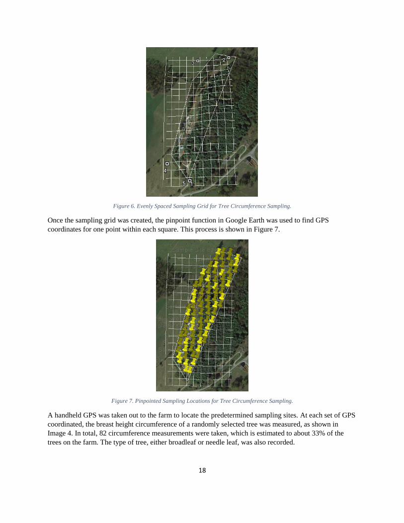
The first step in determining the amount of carbon sequestered by trees on site was to take a random
sample of tree circumferences. To do this, an evenly spaced sampling grid was created using Google
Earth. This sampling grid is shown in Figure 6.
22 http://www.ipcc-nggip.iges.or.jp/public/2006gl/vol4.html
18
Figure 6. Evenly Spaced Sampling Grid for Tree Circumference Sampling.
Once the sampling grid was created, the pinpoint function in Google Earth was used to find GPS
coordinates for one point within each square. This process is shown in Figure 7.
Figure 7. Pinpointed Sampling Locations for Tree Circumference Sampling.
A handheld GPS was taken out to the farm to locate the predetermined sampling sites. At each set of GPS
coordinated, the breast height circumference of a randomly selected tree was measured, as shown in
Image 4. In total, 82 circumference measurements were taken, which is estimated to about 33% of the
trees on the farm. The type of tree, either broadleaf or needle leaf, was also recorded.

19
Image 4. Measurement Method for Tree Circumferences.
Once the circumference measurements were taken, they were logged into an Excel workbook. The
circumference measurement data was converted into corresponding diameter measurements in
centimeters. Once the diameter was known, Equation 3 (for broadleaf) or Equation 4 (for needle leaf) was
used to calculate the amount of carbon stored by the tree.
Equation 3
Equation 4
After calculating how much carbon could be stored by the trees sampled, the amount of carbon dioxide
that could be stored was calculated. This was accomplished by multiplying the amount of carbon stored
by the atomic weight ratio of carbon to carbon dioxide, which is 3.66.
Once the amount of carbon dioxide stored by the trees sampled was calculated, this value was
extrapolated out to estimate the sequestration capabilities of the entire farm.
The carbon sequestration capabilities of the orchard were also calculated. In this case, the circumference
of each tree in the orchard was measured. The methodology for calculating carbon stored is the same, but
only Equation 3 was used because all of the trees in the orchard are broadleaf.
Examining Ways to Reach Net Zero Greenhouse Gas Emissions The final phase of this project was to examine ways to reach net zero greenhouse gas emissions. This
involved a renewable energy assessment and research into ways to increase on site carbon sequestration
capabilities.
Lowering Carbon Dioxide Emissions
The most effective way to lower carbon dioxide emissions is through energy management. The Energy
Management Pyramid, shown in Figure 8, was used as a guide for this portion of the project.

20
Figure 8. The Energy Management Pyramid. (DOE, 2007).
In accordance with this pyramid, energy conservation options were researched first. Next, ways to
improve energy efficiency were research. To see the results of this research, refer to the section of this
report entitled Conservation and Energy Efficiency Results.
Finally, a renewable energy assessment was performed to evaluate potential fuel switching options on
site. Four potential systems were evaluated: a roof mount solar system, a ground mount solar system, a
residential scale wind turbine, and switching to a new rate provided by the farm’s electric utility.
Roof Mount Solar PV System
The first step in assessing the potential for a roof mount solar PV system was selecting a building. The
workhouse was chosen based on the fact that it has a large roof area and contains energy using devices for
the farm.
Once the workhouse was selected, it was modeled in Google SketchUp by following a SketchUp tutorial
in the program’s User Manual. Then, a SketchUp plug-in called Skelion was used to model a solar system
for the roof. This was accomplished using the Skelion User Manual. The SketchUp model of the
workhouse is shown in Figure 9.
Figure 9. Google SketchUp Rendering of the Green Fence Farm Workhouse.

21
In order for the Skelion report to be accurate, it was necessary to determine a shading factor for the
workhouse roof. This was accomplished using a Solar Pathfinder, which is show in Figure 10.
Figure 10. Solar Pathfinder Kit (Solar Pathfinder, 2015)
A Solar Pathfinder was brought out to the farm. The first step in using the Pathfinder is to assemble the
structure, which was done by setting up the tripod and putting the base piece on top. Next, the annual
solar path diagram sheet that corresponded with Green Fence Farm’s latitude was attached to the base.
This structure was then placed on the roof of the workhouse. Next, the instrument section, which is the
clear dome piece shown in Figure 9, was placed on top of the base piece. The level on the instrument
section was used to ensure the Pathfinder was kept level throughout the data taking process. Once the
instrument was level, it was adjusted such that it faced true North according to the compass on the
instrument piece. The reflective dome of the instrument showed the tree profile for the roof, as seen in
Image 5.
Image 5. Photograph of the Solar Pathfinder on the Workhouse Roof.
This profile was traced onto the annual solar path diagram using the chalk provided with the Solar
Pathfinder kit. This profile was used to determine what percentage of the year the roof is shaded. This is
done by adding up the tick marks that on the paper that do not fall within the tree profile for each month.
These tick marks are then summed to determine shade the roof receives each month. Monthly shading
percentages were added and averaged to determine the shading for the year.
Image 6 shows how the Solar Pathfinder data collection was carried out in the field.
22
Image 6. Photograph of Shading Factor Data Collection.
One side of the roof is shaded more than the other, so Solar Pathfinder measurements were taken at each
side and averaged to determine the estimated shading factor for the entire roof. This shading factor was
then put into Skelion. Skelion then used the information from the Google SketchUp model to run a
PVWatts report that predicted the annual generation for the solar system.
Ground Mount Solar PV System
The first step in evaluating a potential ground mount solar PV system was selecting a site. The least
shaded ground area on site was determined to be located in the grazing area, just beyond the raised beds.
This area is shown in Image 7.
Image 7. Location for a Potential Ground Mount Solar PV System.
Once the location was selected, the potential system was analyzed using the same methodology as the
roof mount solar PV system.
Residential Scale Wind Turbine
The first step taken to determine the potential electricity generation for a wind turbine on site was to mine
raw wind measurements using ArcMap. The latitude and longitude of Green Fence Farm were entered
into ArcMap. The following layers were then activated:
Speed at 80m (average, m/s)

23
Elevation (of farm, m)
Speed at 50m (average, m/s)
Speed at 34m (average, m/s)
Speed at 20m (average, m/s)
After activating these layers, the average wind speed, frequency, average power output, Weibull c, and
Weibull k constants were generated. This data was then imported into an Excel file.
All of the raw data from ArcMap was given at a hub height of 80 meters. The data had to be scaled down
to the desired hub height for a turbine on the farm, which is 20 meters. This was done in Excel using
Equation 5, known as the Weibull distribution.
Equation 5
In Equation 5, k is the Weibull k value generated from ArcMap, A is the Weibull c value generated from
ArcMap and v is the wind speed, which increases in intervals of 1 m/s. Next, the 80 meter Weibull curve
(which uses raw data from ArcMap) was plotted alongside the 20m Weibull curve (which uses scaled
data) to verify that they have the same shape with different means
Next, the verified scaled 20 meter data was used to estimate annual generation. First, the number of hours
per year that a certain wind speed occurs was determined by finding the product of the frequency (from
the Weibull distribution) and the total hours in a year. Then, the expected power outputs for a Bergey
Excel 10kW turbine from the Small Wind Certification Council23 were logged into the Excel file. The
energy output was then determined using Equation 6.
Equation 6
The energy output for each wind speed was then converted into kilowatt-hours. The potential energy
outputs for each wind speed in kilo-watt hours was then summed to estimate annual generation from the
turbine.
The manual estimates done using data from ArcMap were then verified using Windographer. To do this,
the Berkey Excel 10kW turbine was selected from Windographer’s wind turbine library. A copy of this
turbine was made in Windographer and the SWCC power output data was inserted into the model. Next,
the copy of the Bergey Excel 10kW turbine was run for a hub height of 20 meters.
Economic Analysis of Renewable Energy Systems
An economic analysis was performed for each renewable energy system evaluated during this phase of
the project. The first step in this process was to determine how much electricity usage would be offset by
the renewable energy system. This was done in Excel by finding the difference between the annual energy
generated by the renewable energy system and the annual electricity consumption for Green Fence Farm.
Next, research was conducted to determine the purchase, installation, operation, and maintenance costs
for each renewable energy system. The information for the solar PV systems was determined through an
e-mail exchange with solar installation company Sigora Solar. The costs for the wind turbine were
determined using the SWCC website23. This cost data, along with electricity usage offset data, were used
to perform several economic analyses to determine the financial viability of each system.
23 http://bergey.com/documents/2012/05/excel-10-swcc-summary-report.pdf

24
Research was also conducted to determine what financial incentives would be available to assist in
funding the renewable energy system’s installation and operation. This research was conducted using the
Database of State Incentives for Renewables and Energy Efficiency24
Simple Payback Period Analysis
The first economic analysis performed was a simple payback period. To do this, the first step was to
determine the annual energy cost savings each system would provide. This was done using Equation 7.
Equation 7
Once the annual energy savings were known, they were inserted into Equation 8 to determine annual net
savings.
Equation 8
The simple payback period analysis was run for the lifetime of the renewable energy system. Payback on
the system occurred in the year that the net savings value first turned positive.
Discounted Payback Period Analysis
Once the simple payback period analysis was performed, it was modified slightly to yield the discounted
payback period. For this analysis, the annual energy savings were escalated on an annual basis using
Equation 9.
Equation 9
In Equation 9, the Electricity Purchase Escalation Rate used came from the Federal Energy Management
Program’s Commercial Electricity Cost Escalation rates25. For the mid-Atlantic region, this escalation
value was 0.59%. In Equation 9, t is the number of years after the installation of the project. Operations
and maintenance costs were escalated using Equation 9 with an escalation rate of 2%.
Once the escalated energy cost savings and operation and maintenance costs were calculated, they were
used in Equation 10 to determine the annual net savings for the renewable energy system.
24 http://www.dsireusa.org/ 25 http://www.nrel.gov/analysis/lcoe/includes/pdfs/us_map_cost_escalations_title.pdf

25
Equation 10
In Equation 10, the discount rate used was 5%. The discounted payback period analysis was run for the
lifetime of the renewable energy system. Payback on the system occurred in the year that the net savings
value first turned positive.
Life Cycle Cost
The life cycle cost for each renewable energy system was calculated using Equation 11.
Equation 11
The usable life varied from system to system.
Greenhouse Gas Offset by Renewable Energy Systems
The first step in determining the amount of greenhouse gas emissions offset by each renewable energy
system was to calculate annual electricity usage savings. This was done in Excel by finding the difference
between the annual energy generated by the renewable energy system and the annual electricity
consumption for Green Fence Farm.
Once the annual electricity savings were determined, Equation 12 was used to calculate the corresponding
carbon dioxide offset.
Equation 12
In Equation 12, the eGRID factor for carbon dioxide for Virginia is 1,624 pounds of CO2 per mega-watt
hour26.
Renewable Energy Option SVEC
The final option that was considered to lower carbon dioxide emissions on the farm was to switch to a
new electricity tariff. Green Fence Farm is serviced by the Shenandoah Valley Electric Cooperative. This
utility offers members the option to purchase 100% of their electricity from renewable energy sources.
This option comes at a cost of an additional $0.015 per kilowatt-hour27. The additional annual cost to
Green Fence Farm was calculated using Equation 13.
Equation 13
The annual carbon dioxide offset from switching to the renewable energy option was calculated using
Equation 12.
Increasing Sequestration Capabilities
When considering ways to increase the carbon sequestration capabilities of Green Fence Farm, three
types of carbon sink were examined: crops, trees, and soil.
26 http://www.epa.gov/cleanenergy/documents/egridzips/eGRID_9th_edition_V1-0_year_2010_GHG_Rates.pdf 27 http://www.svec.coop/Our-Environment/Renewable-Energy-Option-Rider-R.aspx

26
Carbon Sequestration through Crops
Crops on site, much like the trees, can sequester carbon dioxide produce through farming activities.
However, when analyzing the potential to increase carbon sequestration through crops, it was determined
that they are already considered to be net zero because the crop residue is either used on site as animal
feed or sent to the composting facility where Green Fence receives compost from each year. For this
reason, crops were not considered as a way to increase carbon sequestration on site.
Carbon Sequestration through Trees
One option considered to boost carbon sequestration on Green Fence Farm was to plant more trees.
However, this option was eliminated because the property is already 59% forested, and adding more trees
would detract from the ability to farm effectively.
Carbon Sequestration through Soil
The final way to increase sequestration on site that was examined was by adding a soil amendment to the
raised beds and grassland. Biochar was considered for this project. A report published by the Worchester
Polytechnic Institute states that each ton added to soil can store 1.06 tons of carbon dioxide28. The report
also recommends adding between 1 and 5 tons per acre to optimize the benefits of the soil amendment.
These values were used in Equation 14 to estimate the potential increase in sequestration from a biochar
soil amendment.
Equation 14
28 https://www.wpi.edu/Pubs/E-project/Available/E-project-031111-153641/unrestricted/BIOCHAR_CO2SEQ.pdf

27
Results and Analysis
Farm System Analysis After collecting information regarding the inputs, processes, and outputs of Green Fence Farm, a
comprehensive systems diagram was created. This diagram, shown in Image 8, served as a guide for the
entirety of the project.
Image 8. Photograph of Systems Diagram of Green Fence Farm.
This systems diagram considered two types of inputs: human and economic inputs, such as labor and
machinery, as well as physical inputs, such as soil, climate, vegetation, and animals. These inputs
influence the on farm processes such as manure management, land management practices, and product
storage. These farming processes turn the inputs into marketable goods in the form of produce and animal
products.
Current Greenhouse Gas Emissions The current status of emissions on Green Fence Farm is a combination of on farm fuel usage and the
results of the greenhouse gas inventory.
On Farm Fuel Usage
Table 3 shows the fuel usage for a representative year on Green Fence Farm.

28
Table 3. Representative Year of Fuel Consumption for Green Fence Farm.
As Table 3 shows, most of the farm’s energy consumption is in the form of electricity, which powers
essentials such as the electric fences and refrigerators. The next highest consumption is of gasoline, which
is used to operate farm vehicles. The propane usage is the lowest because the generator is only used when
the power goes out.
Figure 11 shows the annual fuel usage patterns on Green Fence Farm.

29
Figure 11. Annual Energy Consumption Patterns for Green Fence Farm.
Electricity consumption on the farm is the most consistent throughout the year, mainly because the load
remains consistent. The gas and propane usage, though, both experience a dramatic spike from May until
about August. Gas usage is highest then because farming operations are in full swing. Propane usage
spikes during the summer because that is when thunderstorms are likely to knock the power out, in which
case Sparks and Auclair use the backup generator.
Table 4 shows the carbon dioxide equivalents that come from electricity, gas, and propane usage on site.
Table 4. Carbon Dioxide Emissions from On Site Fuel Consumption.
As expected, most of the emissions associated with on-site energy usage come from electricity. However,
even though the farm uses less propane annually, it emits more carbon dioxide than the gas used on site.
Despite this, it is not considered to be an energy saving opportunity because it is rarely used. The total
carbon dioxide emissions from on-site fuel consumption is just over 19,000 kilograms per year.
Greenhouse Gas Inventory
The results of the greenhouse gas inventory are shown in Table 5.
Table 5. Greenhouse Gas Inventory Results.

30
31
The greenhouse gas inventory considered both increases in carbon sinks, such as crop growth, and
activities that release carbon, such as soil disturbances.
The manure management at Green Fence Farm releases a total of 761 kilograms of carbon dioxide
equivalents per year. This is one of the highest emitters on the farm, mainly because they have so many
animals on site. That being said, Sparks and Auclair already implement best management practices when
it comes to dealing with the manure created on site. By rotating where their animals graze frequently, they
allow the manure deposited in certain areas to release necessary nutrients back into the soil. This fertilizes
the grazing area, allowing grass to grow back in a quick, healthy manner. Rotating the animals ensures
that the amount of manure in an area does not exceed the amount the ground can handle, preventing
issues like leaching. Therefore, manure management is not considered a greenhouse gas saving
opportunity.
Each year, new growth in the forested land on site sequesters over 75,000 kilograms of carbon dioxide.
However, Sparks and Auclair remove approximately 20 pine trees from their property each year, some of
which is burned for fuel. These biomass removals result in the release of more than 176,000 kilograms of
carbon dioxide per year. However, the removal of these trees is necessary. Trees being removed are either
dead or dying, and therefore do not sequester all that much carbon anyways. Changing the forestry
management practices of Green Fence Farm is not recommended.
The cropland on site, which consists of the raised beds used to grow crops, has very lower carbon storage
and loss rates. This is in part due to the fact that cropland accounts for just 6% of the farm’s land usage.
The emissions associated with cropland are negligible in comparisons to other aspects of the farm and are
therefore not considered a greenhouse gas emissions saving opportunity. The same is true of the
emissions from the grassland.
Green Fence Farm’s emission levels of nitrogen dioxide are also very low. They only use compost in their
raised beds, which has a much lower nitrogen dioxide emission rate than synthetic fertilizers do. This is
also why their indirect nitrogen dioxide emission rates are low; no synthetic fertilizers means there is a
very small amount of nitrogen dioxide leached or volatilized from soils. The largest source of nitrogen
dioxide emissions comes from manure being applied to the grassland, but, as stated earlier, the manure
management at Green Fence Farm is done responsibly and is therefore not a chance to reduce greenhouse
gas emissions.
At the end of the greenhouse gas inventory, the total annual emissions for farming activities in carbon
dioxide equivalents was 163,430 kilograms. This, in combination with the emissions from on-site fuel
consumption, brings the total annual emissions for Green Fence Farm to 182,519 kilograms of carbon
dioxide.
Current Carbon Sequestration Capabilities The carbon sinks on Green Fence Farm the soil and the trees.
Soil Sequestration
The carbon sequestration capabilities of the soil on site were calculated during the greenhouse gas
inventory. The results for soil carbon sequestration and losses are presented in Table 5. Each year, the
forested areas of Green Fence Farm lose 18,274 kilograms of carbon through drained organic soils. The
cropland sequesters 2,593 kilograms of carbon in year in mineral soils, but loses 26,874 kilograms of
carbon dioxide through soil cultivation. The mineral soils in the grassland of the farm sequester 24,126
32
kilograms of carbon dioxide annually, but grassland soil disturbances release 40,311 kilograms of carbon
dioxide. Soil management practices result in both direct and indirect nitrogen dioxide emissions. These
emissions total 55 kilograms of carbon dioxide equivalents each year.
As previously stated, the annual soil carbon sequestration and losses are part of the greenhouse gas
inventory. Therefore, they have already been accounted for in the total annual emissions for Green Fence
Farm.
Tree Sequestration
Table 6 provides a sample of the data collected during the tree sequestration analysis.
Table 6. Sample of Data for Carbon Dioxide Stored by Trees on Site.
Site Number TypeCircumference
(in)
Diameter
(in)
Diameter
(cm)
Stored Carbon
(kg)
Stored Carbon Dioxide
(kg)
Sample Site 1 Needleleaf 38 12.10 30.74 103.83 380.69
Sample Site 2 Needleleaf 51 16.24 41.25 222.34 815.16
Sample Site 3 Needleleaf 47 14.97 38.02 180.45 661.60
Sample Site 4 Needleleaf 36 11.46 29.12 90.07 330.22
Sample Site 5 Needleleaf 56 17.83 45.30 281.42 1031.76
Sample Site 6 Needleleaf 53.5 17.04 43.28 250.95 920.08
Sample Site 7 Broadleaf 23 7.32 18.61 37.57 137.75
Sample Site 8 Broadleaf 26 8.28 21.03 50.94 186.76
Sample Site 9 Broadleaf 10 3.18 8.09 4.71 17.26
Sample Site 10 Broadleaf 66 21.02 53.39 486.24 1782.71
Sample Site 11 Needleleaf 47 14.97 38.02 180.45 661.60
Sample Site 12 Needleleaf 14 4.46 11.32 7.19 26.37
Sample Site 13 Needleleaf 49 15.61 39.64 200.79 736.17
Sample Site 14 Needleleaf 52 16.56 42.06 233.56 856.31
Sample Site 15 Needleleaf 19 6.05 15.37 16.36 59.99
During the tree sampling, the circumferences of 73 needle leaf trees were recorded. The circumference
measurements for seven broad leaf trees were also taken. The minimum diameter at breast height (DBH)
for the trees sampled was 6.5 centimeters, while the maximum was 57.4 centimeters. The average DBH
for all of the trees sampled was 32 centimeters.
The minimum amount of carbon dioxide stored by one tree was 9.8 kilograms, while the maximum was
2,106 kilograms. The average carbon dioxide storage for the trees sampled was 542 kilograms. The trees
sampled can store a total of 42,863 kilograms of carbon dioxide. This value was extrapolated out and it is
estimated that the trees on the farm can store 128,589 kilograms of carbon dioxide.
The carbon sequestration capabilities of the small orchard site were also calculated. It is estimated that the
orchard occupies 0.06 acres on the farm. According to a study published by the New York State
Horticultural Society, an orchard can store 20 tons of carbon dioxide per acre. Therefore, the orchard at
Green Fence Farm can sequester approximately 1,088 kilograms of carbon dioxide each year. This, when
combined with the carbon dioxide sequestered by the other trees on site, results in an annual carbon
dioxide sequestration of 129,678 kilograms.
Ways to Reach Net Zero Greenhouse Gas Emissions Table 7 describes the current state of emissions and sequestration on Green Fence Farm.
Table 7. Current State of Greenhouse Gas Emissions and Sequestration for Green Fence Farm.

33
Green Fence Farm currently emits 182,519 kilograms of carbon dioxide annually. However, they store
only 129,678 kilograms of carbon dioxide on site each year. Therefore, Green Fence Farms currently
emits 52,841 more kilograms of carbon dioxide each year than it stores. To get the farm to net zero,
emissions need to be lowered and sequestration capabilities need to be increased.
Lowering Carbon Dioxide Emissions
The first step in reaching net zero greenhouse gas emissions is to reduce the amount of carbon dioxide
being emitted on site. This can be done through conservation, energy efficiency improvements, and fuel
switching, as shown in the Energy Management Pyramid in Figure 8.
Conservation Results
The first consideration when trying to improve the energy usage on a farm is to implement conservation
methods. Reducing the amount of energy used is a cost effective way to save money on annual energy
costs, as well as lower emissions. Additionally, it is a crucial step for sizing renewable energy systems,
which will discussed later in this section.
When considering ways for Green Fence Farm to conserve energy, the following list of recommendations
was compiled:
Do not condition spaces when they are not being used.
Turn off appliances when they are not being used.
When possible, perform farming activities such as planting, watering, weeding, and harvesting by
hand.
Switch to a low or no till land management strategy, which helps reduce energy usage and losses
from soil disturbances.
However, all of these recommendations are already being implemented on Green Fence Farm. The only
conditioned workspace is the workhouse, and when it is not in use, it is not being conditioned. Appliances
are unplugged when they are not in use. Almost all farming activities are already performed by hand and
they implement a low-till management strategy. Therefore, Green Fence Farm is already performing well
in the area of energy conservation and there are no recommendations to be made for improvement.
34
Energy Efficiency Results
The next consideration when attempting to improve energy usage is to make energy efficiency
improvements. When considering ways for farms to improve energy efficiency, energy consumption in
the following areas are examined:
Irrigation
Fertilizer Usage
Greenhouse Operations
Farm Vehicles
Appliances
Lighting
Green Fence Farm does not have an irrigation system, does not use fertilizer, and does not have a
greenhouse. Therefore, there are no energy efficiency improvements to be made in those categories.
As for farm vehicles, Green Fence Farm could switch to more fuel efficient vehicles than the ones
currently used. However, farm vehicles are used so sparingly on site that any emissions and energy cost
savings from purchasing a new vehicle would not be financially justified.
When it comes to appliances, the best way to increase energy efficiency is to switch to Energy Star
products. All of the freezers and refrigerators on site, though, are already Energy Star. Therefore, there
are not any energy efficiency recommendations for the appliances category.
The majority of the workspaces on Green Fence Farm are open sheds which are lit via sunlight. The
workhouse, which is used to start seedlings, however, does currently use fluorescent lighting. Switching
these bulbs to LEDs would help reduce electricity usage and consequently greenhouse gas emissions.
This reduction, however, would be almost insignificant when compared the emissions from the rest of the
farming activities.
Once conservation and energy efficiency measures were considered, renewable energy options for the site
were evaluated as potential ways to offset the rest of the carbon dioxide emissions.
Roof Mount Solar PV System
Figure 12 shows the roof mount solar PV system modelled in Google SketchUp using Skelion.

35
Figure 12. Roof Mount Solar PV System Rendering.
This is a 9kW roof mount system. The shading profile determine using the Solar Pathfinder is show in
Image 9.
Image 9. Solar Pathfinder Shading Profile for Workhouse Roof.
The data from the Solar Pathfinder shading analysis was logged in Excel and used to estimate the shading
de-rate factor for the roof. The estimated shading de-rate factor for the workhouse roof was 35%.
Skelion used this shading de-rate factor and estimated the annual generation for the roof mount solar PV
system. Monthly generation estimates are presented in Table 8.
Table 8. Estimated Electricity Generation for a Roof Mount Solar PV System.
36
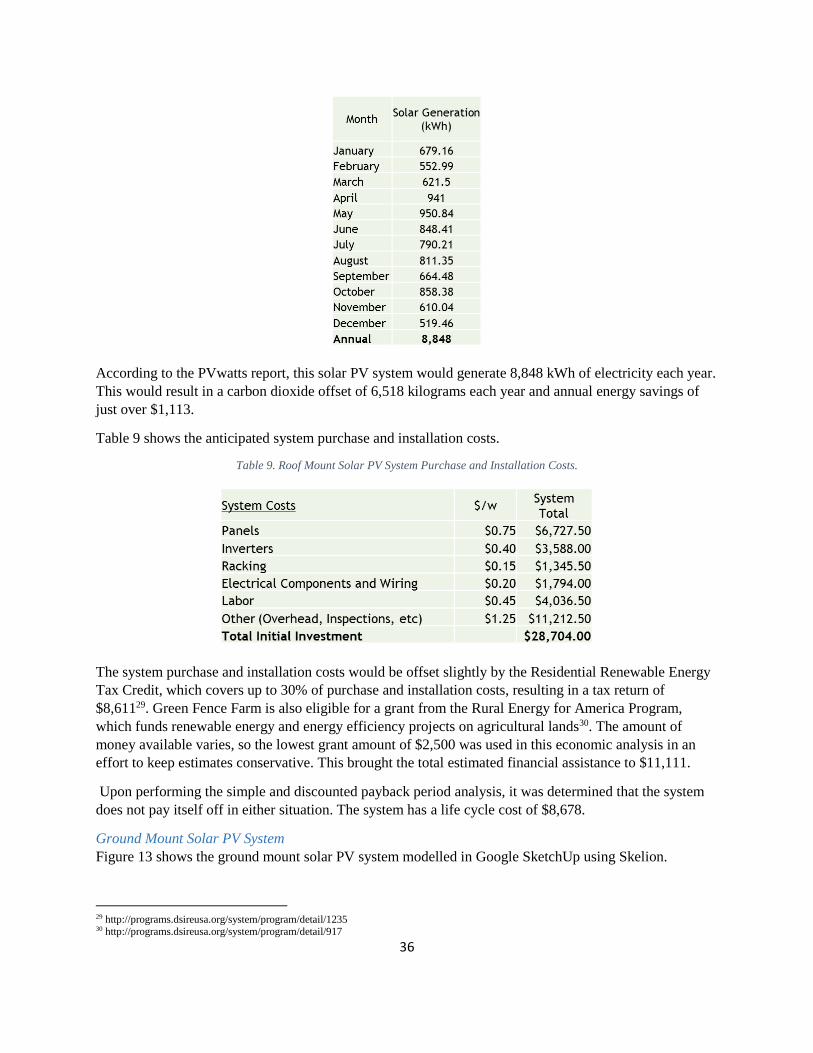
According to the PVwatts report, this solar PV system would generate 8,848 kWh of electricity each year.
This would result in a carbon dioxide offset of 6,518 kilograms each year and annual energy savings of
just over $1,113.
Table 9 shows the anticipated system purchase and installation costs.
Table 9. Roof Mount Solar PV System Purchase and Installation Costs.
The system purchase and installation costs would be offset slightly by the Residential Renewable Energy
Tax Credit, which covers up to 30% of purchase and installation costs, resulting in a tax return of
$8,61129. Green Fence Farm is also eligible for a grant from the Rural Energy for America Program,
which funds renewable energy and energy efficiency projects on agricultural lands30. The amount of
money available varies, so the lowest grant amount of $2,500 was used in this economic analysis in an
effort to keep estimates conservative. This brought the total estimated financial assistance to $11,111.
Upon performing the simple and discounted payback period analysis, it was determined that the system
does not pay itself off in either situation. The system has a life cycle cost of $8,678.
Ground Mount Solar PV System
Figure 13 shows the ground mount solar PV system modelled in Google SketchUp using Skelion.
29 http://programs.dsireusa.org/system/program/detail/1235 30 http://programs.dsireusa.org/system/program/detail/917

37
Figure 13. Ground Mount Solar PV System Rendering.
This is a 12kW ground mount system. The shading profile determine using the Solar Pathfinder is show
in Image 10.
Image 10. Solar Pathfinder Shading Profile for Ground Mount System Location.
The data from the Solar Pathfinder shading analysis was logged in Excel and used to estimate the shading
de-rate factor for the ground mount system. The estimated shading de-rate factor was 32%.
Skelion used this shading de-rate factor and estimated the annual generation for the ground mount solar
PV system. Monthly generation estimates are presented in Table 10.

38
Table 10. Estimated Electricity Generation for a Ground Mount Solar PV System.
According to the PVwatts report, this solar PV system would generate 9,893 kWh of electricity each year.
This would result in a carbon dioxide offset of 7,287 kilograms each year and annual energy savings of
just over $1,217.
Table 11 shows the anticipated system purchase and installation costs.
Table 11. Ground Mount Solar PV System Purchase and Installation Costs.
The purchase and installation costs for the ground mount system are inherently higher than the roof mount
system because installing a ground mount system requires additional labor for trenching and wiring. In
this case, the Residential Renewable Energy Tax Credit would result in a return of $14,40031. REAP
funding could also be used for the ground mount system and the lowest award of $2,500 was used in this
economic analysis to keep estimates conservative. This brought the total estimated financial assistance to
$16,900.
Upon performing the simple and discounted payback period analysis, it was determined that the system
does not pay itself off in either situation. The system has a life cycle cost of $25,168.
31 http://programs.dsireusa.org/system/program/detail/1235

39
Residential Scale Wind Turbine
Table 12 provides the raw data for average wind speed, Weibull c, and Weibull k constants that was
generated in ArcMap.
Table 12. Average Wind Speeds and Weibull Constants from ArcMap.
Speed 80m 4.95
Speed 50m 4.58
Speed 34m 4.30
Speed 20m 3.94
Weibull C 5.6
Weibull K 2.2
Average Wind Speed (m/s)
Weibull Constants
AcrMap also generated a Weibull distribution at an 80m hub height, which is shown in Table 13.
Table 13. Weibull Distribution for an 80m Hub Height.
Bin Speed (m/s) Frequency (%)
FREQ00T01 1 0.035
FREQ01T02 2 0.087
FREQ02T03 3 0.115
FREQ03T04 4 0.139
FREQ04T05 5 0.156
FREQ05T06 6 0.151
FREQ06T07 7 0.118
FREQ07T08 8 0.084
FREQ08T09 9 0.057
FREQ09T10 10 0.033
FREQ10T11 11 0.017
FREQ11T12 12 0.005
FREQ12T13 13 0.002
FREQ13T14 14 0.001
FREQ14T15 15 0
FREQ15T16 16 0
FREQ16T17 17 0
FREQ17T18 18 0
FREQ18T19 19 0
FREQ19T20 20 0
FREQGT20 21 0
Weibull at 80m
The 80m hub height data was scaled down to 20m using the Weibull constants from Table 12 and
Equation 5. The scaled data is presented in Table 14.

40
Table 14. Estimated Weibull Distribution for a 20m Hub Height.
Speed (m/s) Frequency (%)
1 0.0509
2 0.1054
3 0.1455
4 0.1625
5 0.1557
6 0.1313
7 0.0986
8 0.0663
9 0.0402
10 0.0219
11 0.0108
12 0.0048
13 0.0019
14 0.0007
15 0.0002
16 0.0001
17 0.0000
18 0.0000
19 0.0000
20 0.0000
21 0.0000
Weibull at 20m
The data from Tables 13 and 14 were graphed. This was to verify that the Weibull distribution for a 20m
hub height had the same shape as the Weibull distribution for the 80m hub height, but with a different
mean. This graph, shown in Figure 14, verified that the scaled down Weibull distribution was reasonable.
41
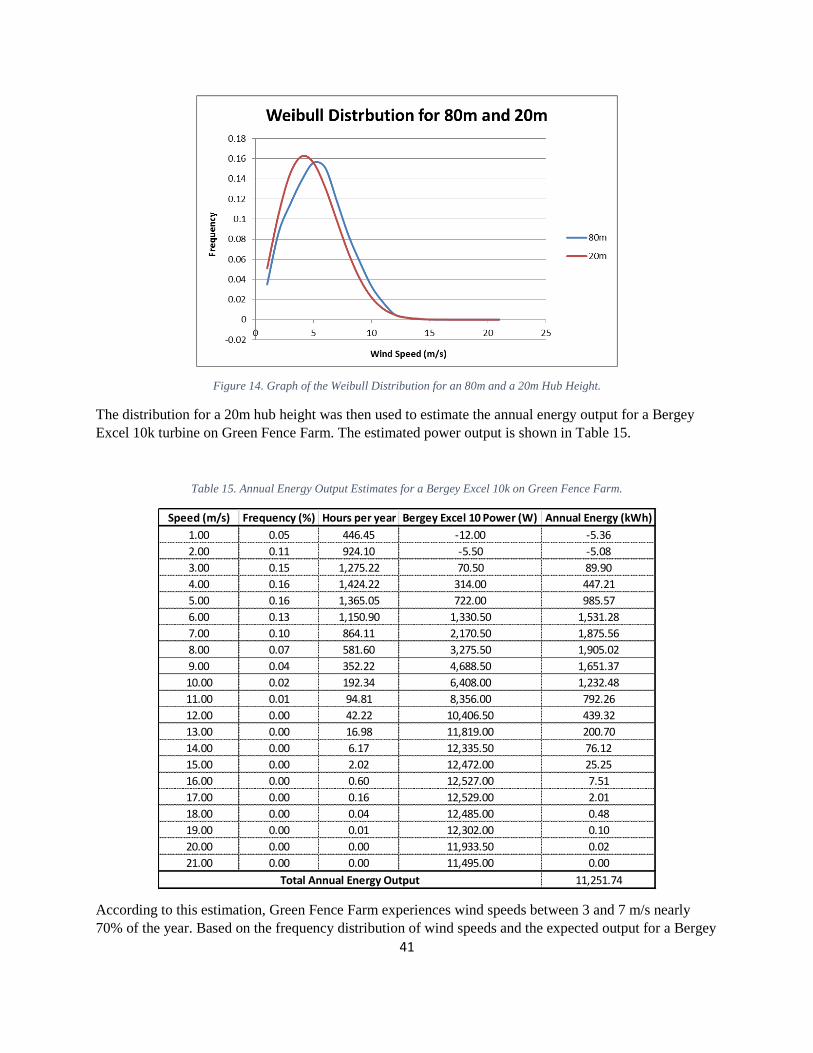
Figure 14. Graph of the Weibull Distribution for an 80m and a 20m Hub Height.
The distribution for a 20m hub height was then used to estimate the annual energy output for a Bergey
Excel 10k turbine on Green Fence Farm. The estimated power output is shown in Table 15.
Table 15. Annual Energy Output Estimates for a Bergey Excel 10k on Green Fence Farm.
Speed (m/s) Frequency (%) Hours per year Bergey Excel 10 Power (W) Annual Energy (kWh)
1.00 0.05 446.45 -12.00 -5.36
2.00 0.11 924.10 -5.50 -5.08
3.00 0.15 1,275.22 70.50 89.90
4.00 0.16 1,424.22 314.00 447.21
5.00 0.16 1,365.05 722.00 985.57
6.00 0.13 1,150.90 1,330.50 1,531.28
7.00 0.10 864.11 2,170.50 1,875.56
8.00 0.07 581.60 3,275.50 1,905.02
9.00 0.04 352.22 4,688.50 1,651.37
10.00 0.02 192.34 6,408.00 1,232.48
11.00 0.01 94.81 8,356.00 792.26
12.00 0.00 42.22 10,406.50 439.32
13.00 0.00 16.98 11,819.00 200.70
14.00 0.00 6.17 12,335.50 76.12
15.00 0.00 2.02 12,472.00 25.25
16.00 0.00 0.60 12,527.00 7.51
17.00 0.00 0.16 12,529.00 2.01
18.00 0.00 0.04 12,485.00 0.48
19.00 0.00 0.01 12,302.00 0.10
20.00 0.00 0.00 11,933.50 0.02
21.00 0.00 0.00 11,495.00 0.00
11,251.74Total Annual Energy Output
According to this estimation, Green Fence Farm experiences wind speeds between 3 and 7 m/s nearly
70% of the year. Based on the frequency distribution of wind speeds and the expected output for a Bergey
42
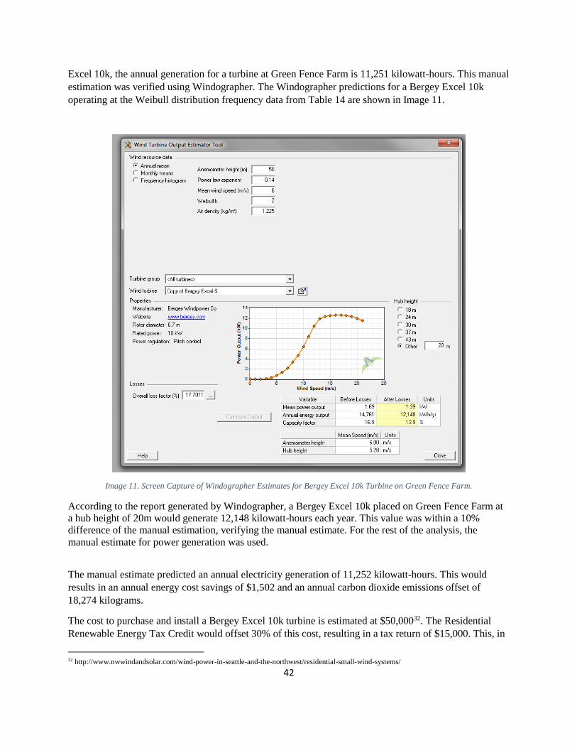
Excel 10k, the annual generation for a turbine at Green Fence Farm is 11,251 kilowatt-hours. This manual
estimation was verified using Windographer. The Windographer predictions for a Bergey Excel 10k
operating at the Weibull distribution frequency data from Table 14 are shown in Image 11.
Image 11. Screen Capture of Windographer Estimates for Bergey Excel 10k Turbine on Green Fence Farm.
According to the report generated by Windographer, a Bergey Excel 10k placed on Green Fence Farm at
a hub height of 20m would generate 12,148 kilowatt-hours each year. This value was within a 10%
difference of the manual estimation, verifying the manual estimate. For the rest of the analysis, the
manual estimate for power generation was used.
The manual estimate predicted an annual electricity generation of 11,252 kilowatt-hours. This would
results in an annual energy cost savings of $1,502 and an annual carbon dioxide emissions offset of
18,274 kilograms.
The cost to purchase and install a Bergey Excel 10k turbine is estimated at $50,00032. The Residential
Renewable Energy Tax Credit would offset 30% of this cost, resulting in a tax return of $15,000. This, in
32 http://www.nwwindandsolar.com/wind-power-in-seattle-and-the-northwest/residential-small-wind-systems/

43
combination with the lowest grant amount provided by REAP, would result in a total financial assistance
of $17,500.
Upon performing the simple and discounted payback period analysis, it was determined that the system
does not pay itself off in either situation. The system has a life cycle cost of $21,749.
Renewable Energy Option from SVEC
It would be possible for Green Fence Farm to offset all electricity used on site by switching to the
renewable energy option provided by SVEC. During the on-site fuel usage evaluation, it was determined
that in a typical year, Green Fence Farm uses 25,304 kilowatt-hours. Purchasing all of this energy from
renewable energy sources would offset 18,641 kilograms of carbon dioxide each year. The additional cost
for this electricity tariff would be just below $380 each year, as shown in Table 26.
Table 16. Additional Cost to Purchase Electricity from Renewable Energy Projects.
Increasing Sequestration Capabilities
The other step that can be taken to help Green Fence Farm reach net zero greenhouse gas emissions is to
increase sequestration capabilities on site.
Sequestration in Soil
The carbon sequestration capabilities of a biochar soil amendment were examined as a way to increase the
amount of carbon dioxide stored on site. To optimize the benefits provided by biochar, three tons should
be applied per acre of crop and grassland. This would result in a total of 20.9 tons of biochar being added
to the soil. One ton of biochar can sequester 1.06 tons of carbon dioxide, so this soil amendment would
increase the amount of carbon dioxide stored in the soil by 20,286 kilograms. Biochar can be purchased at
a price of $40 per ton, so the total cost for this carbon sequestration increase would be just below $840.
Sequestration in Biomass
As previously stated, the crops on site are already considered to have net zero greenhouse gas emissions
and therefor are not an opportunity to increase sequestration. Planting more trees to increase sequestration
was also not considered because doing so would detract from the ability to farm the land.

44
Purchasing Carbon Offsets
The final strategy examined to reach net zero greenhouse gas operations was the purchase of carbon
offsets. Essentially, by purchasing carbon offsets, Green Fence Farm can offset the rest any remaining
emissions by investing in renewable energy projects elsewhere. Carbon offsets can be purchased for an
average of $5.95 per 1000 pounds of carbon dioxide. Any excess emissions that need to be offset after the
Green Fence Farm implements the recommendations from this project will be addressed through the
purchasing of carbon offsets.
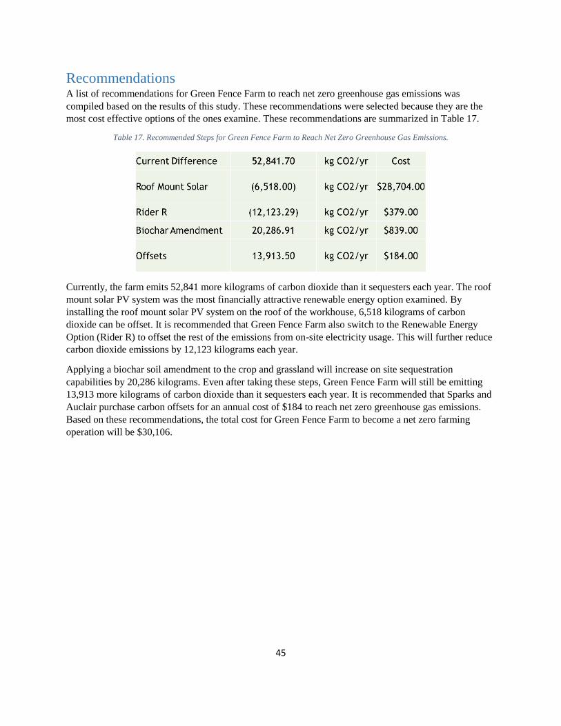
45
Recommendations A list of recommendations for Green Fence Farm to reach net zero greenhouse gas emissions was
compiled based on the results of this study. These recommendations were selected because they are the
most cost effective options of the ones examine. These recommendations are summarized in Table 17.
Table 17. Recommended Steps for Green Fence Farm to Reach Net Zero Greenhouse Gas Emissions.
Currently, the farm emits 52,841 more kilograms of carbon dioxide than it sequesters each year. The roof
mount solar PV system was the most financially attractive renewable energy option examined. By
installing the roof mount solar PV system on the roof of the workhouse, 6,518 kilograms of carbon
dioxide can be offset. It is recommended that Green Fence Farm also switch to the Renewable Energy
Option (Rider R) to offset the rest of the emissions from on-site electricity usage. This will further reduce
carbon dioxide emissions by 12,123 kilograms each year.
Applying a biochar soil amendment to the crop and grassland will increase on site sequestration
capabilities by 20,286 kilograms. Even after taking these steps, Green Fence Farm will still be emitting
13,913 more kilograms of carbon dioxide than it sequesters each year. It is recommended that Sparks and
Auclair purchase carbon offsets for an annual cost of $184 to reach net zero greenhouse gas emissions.
Based on these recommendations, the total cost for Green Fence Farm to become a net zero farming
operation will be $30,106.

46
Conclusions In conclusion, reaching net zero greenhouse gas emissions is a challenging and potentially costly goal.
However, it is a process that is going to become increasingly necessary in the future. The world’s
population is projected to surpass 9 billion people by 205033. This means that there will be 2 billion more
mouths to feed and a continually diminishing amount of resources to use. If the greenhouse gas emissions
associated with the agricultural sector are not reduced, then the effects of global warming will continue to
worsen, severely impacting the world’s food supply chain. If, however, less greenhouse gas intensive
farming practices are adopted worldwide, then perhaps the world’s population can be fed without
destroying the resources required for food production. Agricultural operations like Green Fence Farm
represent an opportunity to develop a model for sustainable, environmentally friendly food production
that could one day feed the planet.
33 http://news.nationalgeographic.com/news/2013/13/1307011-population-census-united-nations-un-demographics-world-population-day-birthrate/

47
Bibliography
"Agriculture." EPA. Environmental Protection Agency, Apr. 2015. Web. 05 May 2015.
"The Benefits of Farm to School." (n.d.): n. pag. Farm to School Network. Web.
Ch06, Ddb. Biochar Production for Biochar Sequestration (n.d.): n. pag. Worcester Polytechnic
Institute, Mar. 2011. Web.
Database of State Incentives for Renewables & Efficiency. US Department of Energy, n.d. Web. 05
May 2015.
DeCapua, Joe. "More Land Being Used for Organic Farming." VOA. N.p., Jan. 2013. Web. 05 May
2015.
Driesen, David M. "Review: Post-Kyoto International Climate Policy: Summary for
Policymakers." Perspectives on Politics 9.1 (2011): 123-24. Intergovernmental Panel on Climate
Change, 2014. Web.
"Economic Analysis Reveals Organic Farming Profitable Long-term." ScienceDaily. ScienceDaily,
Sept. 2011. Web. 05 May 2015.
EGRID 9th Edition Version 1.0 GHG Annual Output Emission Rates for Year 2010 Data (n.d.): n. pag.
Environmental Protection Agency, 2010. Web.
"FAQ for Residential Small Wind Systems." NW Wind & Solar. N.p., n.d. Web. 05 May 2015.
FEMP Commercial Electricity Cost Escalation Rates for 25-Year Analysis for 2013 (n.d.): n. pag.
Federal Energy Management Program. Web.
"Global Climate Change: Evidence." Climate Change: Vital Signs of the Planet. NASA, n.d. Web. 05
May 2015.
Gogi, Pallavi. "The Rise of the 'Locavore'" Bloomberg.com. Bloomberg Business, May 2008. Web. 05
May 2015.
Low, Sarah A. Trends in U.S. Local and Regional Food Systems: A Report to Congress (n.d.): n. pag.
United States Department of Agriculture, Jan. 2015. Web.
48
Maiser, Jennifer. "10 Steps to Becoming a Locavore." PBS. PBS, Nov. 2007. Web. 05 May 2015.
"Market Forces: Creating Jobs through Public Investment in Local and Regional Food Systems." (n.d.):
n. pag. Union of Concerned Scientists, Aug. 2011. Web.
Molla, Rani. "Can Organic Farming Counteract Carbon Emissions?" The Wall Street Journal, 2014.
Web. 05 May 2015.
Opportunities to Reduce Greenhouse Gas Emissions through Materials and Land Management
Practices. Washington, DC: U.S. Environmental Protection Agency, Office of Soild Waste and
Emergency Response, 2009. Environmental Protection Agency, Sept. 2009. Web.
"Organic Agriculture: What Are the Environmental Benefits of Organic Agriculture?" Food and
Agriculture Organizations of the United Nations, 2015. Web. 05 May 2015.
"Renewable Energy Option - Rider R." Shenandoah Electric Cooperative. N.p., n.d. Web. 05 May
2015.
Skurie, Jaclyn. "Unpacking 9.6 Billion by 2050." National Geographic. National Geographic Society,
July 2013. Web. 05 May 2015.
Smith, James E., and Linda S. Heath. "Emission Factors for Greenhouse Gas Inventories." (n.d.): n.
pag. Environmental Protection Agency, Apr. 2014. Web.
T. "SWCC Summary Report Bergey Excel 10k." (n.d.): n. pag. Small Wind Certification Council,
2012. Web.
"2006 IPCC Guidelines for National Greenhouse Gas Inventories." Intergovernmental Panel on
Climate Change, 2014. Web. 05 May 2015.
2007, November. NRDC: Food Miles: How Far Your Food Travels Has Serious Consequences for
Your Health and the Climate (pdf) (n.d.): n. pag. Natural Resource Defense Council, Nov. 2007.
Web.
"U.N. Raises "Low" Population Projection for 2050." Worldwatch Institute, n.d. Web. 05 May 2015.
"Unraveling the Complex Web of Global Food Trade." Institute on the Environment. University of
Minnesota, 11 Feb. 2015. Web. 05 May 2015.

49
U.S. Climate Action Report. N.p.: n.p., n.d. United States Department of State, June 2010. Web.
Us Epa, Oar, Climate Change Division. Inventory of U.S. Greenhouse Gas Emissions and Sinks: 1990-
2012 – Agriculture (n.d.): n. pag. Environmental Protection Agency. Web.