a nested mixture model for protein identification...

Submitted to the Annals of Applied Statistics

A NESTED MIXTURE MODEL FOR PROTEIN

IDENTIFICATION USING MASS SPECTROMETRY

By Qunhua Li‡,∗ , Michael MacCoss∗ and Matthew Stephens†

University of Washington∗ and University of Chicago†

Mass spectrometry provides a high-throughput way to identify

proteins in biological samples. In a typical experiment, proteins in a

sample are first broken into their constituent peptides. The resulting

mixture of peptides is then subjected to mass spectrometry, which

generates thousands of spectra, each characteristic of its generat-

ing peptide. Here we consider the problem of inferring, from these

spectra, which proteins and peptides are present in the sample. We

develop a statistical approach to the problem, based on a nested

mixture model. In contrast to commonly-used two-stage approaches,

this model provides a one-stage solution that simultaneously identifies

which proteins are present, and which peptides are correctly identi-

fied. In this way our model incorporates the evidence feedback be-

tween proteins and their constituent peptides. Using simulated data

and a yeast dataset, we compare and contrast our method with ex-

isting widely-used approaches (PeptideProphet/ProteinProphet) and

with a recently-published new approach, HSM. For peptide identifi-

cation, our single-stage approach yields consistently more accurate

results. For protein identification the methods have similar accuracy

in most settings, although we exhibit some scenarios in which the

existing methods perform poorly.

‡Corresponding author. Current address: Department of Statistics, University of Cali-

fornia, 444 Evans, Mail Stop 3860, Berkeley, CA 94720. Email: [email protected]

Keywords and phrases: mixture model, nested structure, EM algorithm, protein iden-

tification, peptide identification, mass spectrometry, proteomics

1

http://www.imstat.org/aoas/

2 LI, MACCOSS AND STEPHENS

1. Introduction. Protein identification using tandem mass spectrome-

try (MS/MS) is the most widely used tool for identifying proteins in complex

biological samples (Steen and Mann, 2004). In a typical MS/MS experiment

(Figure 1a), proteins in a sample are first broken into short sequences, called

peptides, and the resulting mixture of peptides is subjected to mass spec-

trometry to generate tandem mass spectra, which contains sequence infor-

mation that is characteristic of its generating peptide (Coon et al., 2005;

Kinter and Sherman, 2003). The peptide that is most likely to generate

each spectrum then is identified using some computational methods, e.g. by

matching to a list of theoretical spectra of peptide candidates. From these

putative peptide identifications, the proteins that are present in the mix-

ture are then identified. The protein identification problem is challenging,

primarily because the matching of spectra to peptides is highly error-prone:

80-90% of identified peptides may be incorrect identifications if no filtering

is applied (Keller, 2002; Nesvizhskii and Aebersold, 2004). In particular,

to minimize errors in protein identifications it is critical to assess, and take

proper account of, the strength of the evidence for each putative peptide

identification.

Here we develop a statistical approach to this problem, based on a nested

mixture model. Our method differs from most previous approaches to the

problem in that it is based on a single statistical model that incorporates

latent variables indicating which proteins are present, and which peptides

are correctly identified. Thus, instead of taking the more common sequen-

tial approach to the problem (spectra → peptides → proteins), our model

simultaneously estimates which proteins are present, and which peptides are

A NESTED MIXTURE MODEL FOR PROTEIN IDENTIFICATION 3

correctly identified, allowing for appropriate evidence feedback between pro-

teins and their constituent peptides. This not only provides the potential for

more accurate identifications (particularly at the peptide level), but, as we

illustrate here, it also allows for better calibrated estimates of uncertainty

in which identifications are correct. As far as we are aware, the only other

published method that takes a single-stage approach to the problem is that

of Shen et al (Shen et al., 2008). Although Shen et al’s model shares the goal

of our approach of allowing evidence feedback from proteins to peptides, the

structure of their model is quite different from ours (see Discussion for more

details), and, as we see in our comparisons, the empirical performance of the

methods can also differ substantially.

In general statistical terms this problem involves a nested structure of a

form that is encountered in other statistical inference problems (e.g. multi-

level latent class models (Vermunt, 2003), hierarchical topic models (Blei, Gri, Jordan, and Tenenbaum,

2004)). These problems usually share two common features: (1) there exists

a physical or latent hierarchical relationship between lower-level and upper-

level elements; and (2) only the lowest-level elements in the hierarchy are

typically observed. Here the nested structure is due to the subsequence re-

lationship between lower-level elements (peptides) and upper-level elements

(proteins) (Figure 1b). The goals of inference will, of course, vary depending

on the application. In this case the primary goal is to infer the states (i.e.

presence or absence in the mixture) of the upper-level elements, though the

states of the lower-level elements is also of interest.

The structure of the paper is as follows. Section 2 describes the problem

in more detail, reviews existing approaches, and describes our modeling ap-


proach. Section 3 shows empirical comparisons of our method with different

approaches on both real and simulated data. In section 5 we conclude and

discuss potential future enhancements.

2. Methods and Models. The first step in analysis of MS/MS data

is typically to identify, for each spectrum produced, the peptide that is

most likely to have generated the observed spectrum, and to assign each

such identification a score that reflects the strength of the evidence for the

identification being correct. Often this process is performed by searching a

database of potential peptides, and computing some measure of the similar-

ity between the observed spectrum and a theoretical “expected” spectrum

for each peptide in the database (e.g. (Sadygov, Liu, and Yates, 2004)). For

each spectrum the highest-scoring peptide is then reported, together with

its score. Here we assume that this process has already been performed, and

tackle the protein identification problem: using the list of putative peptides,

and scores, to infer a list of proteins that are likely to be present in the

mixture. Other important goals include accurately assessing confidence for

each protein identification, and inferring which of the initial putative peptide

identifications are actually correct.

2.1. Existing approaches. Almost all current approaches to protein iden-

tification follow a two-stage strategy:

1. The peptide identification scores are processed, together with other

relevant information (e.g. sequence characteristics) on the identified

peptide, to compute a statistical measure of the strength of evidence

for each peptide identification. Although several methods exist (e.g.


(Sadygov and Yates, 2003; Kall, Canterbury, Weston, and Noble, 2007)),

by far the most widely used approach appears to be PeptideProphet

(Keller, Nesvizhskii, Kolker, and Aebersold, 2002), which uses a mix-

ture model to cluster the identified peptides into correct and incorrect

identifications, and to assign a probability to each peptide identifica-

tion being correct.

2. The statistical measures of support for each peptide identification are

taken as input to a protein inference procedure. These procedures infer

the presence or absence of each protein, either by simple ad hoc thresh-

olding rules, e.g. identifying proteins as present if they contain two or

more peptides with strong support, or by more sophisticated means

(ProteinProphet (Nesvizhskii, Keller, Kolker, and Aebersold, 2003), Prot Probe

(Sadygov, Liu, and Yates, 2004) and EBP (Price, 2007)). The basic

idea of ProteinProphet (Nesvizhskii et al., 2003), which is the most

widely used of these methods, will be described below.

This two-stage approach, although widely used, is sub-optimal. In partic-

ular, it does not allow for evidence to feed back, from the presence/absence

status of a protein to the status of its constituent peptides, as it should

due to the nested relationship between a protein and its peptides. Shen et

al (Shen, Wang, Shankar, Zhang, and Li, 2008) also note this problem with

the two-stage approach, and propose an alternative one-stage approach us-

ing a latent-variable-based model. Their model differs from ours in several

aspects (see discussion), and performs less well than our approach in the

limited empirical comparisons we consider here (see results).


PeptideProtein Spectrum

Experimental process

Peptide identificationProtein identification

Peptide

Spectrum

Protein AbsentProteins

PresentProteins

a b c

Fig 1. (a) Protein identification using mass spectrometry. Proteins (left) are broken intoconstituent peptides (center), which are then subjected to mass spectrometry to producespectra (right). The inference problem considered here is to infer which peptides, belong-ing to which proteins, generated the observed spectra. (b) Graphical representation of thenested relationship between spectra, peptides and proteins. (c) Examples of putative proteinidentifications reconstructed from putative peptide identifications. Proteins that are trulyabsent from the sample will contain all incorrectly identified peptides (black). Proteins thatare present in the sample will typically contain a mixture of correctly (red) and incorrectly(black) identified peptides.

2.2. A nested mixture model. The data consist of a large number of pu-

tative peptide identifications, each corresponding to a single MS/MS spec-

trum, and each having a score that relates to the strength of the evidence

for the identification being correct (higher scores corresponding to stronger

evidence). From this list of putative peptides, it is straightforward to (deter-

ministically) create a list of putative protein identifications. Specifically, for

each putative peptide identification it is straightforward to determine, from

a protein database, which proteins contain that peptide. The information

available can thus be arranged in a hierarchical structure: a list of N puta-

tive protein identifications, with the information on protein k being a list

of nk putative peptide identifications, with a corresponding vector of scores

xk = (xk,1, . . . , xk,nk). Here xk,j is a scalar score that reflects how well the

spectrum associated with peptide j in protein k matches a theoretical expec-

tation under the assumption that it was indeed generated by that peptide.

(Typically there are also other pieces of information that are relevant in


assessing the evidence for peptide j having generated the spectrum, but we

defer consideration of these to Section 2.5 below.) In general, correct pep-

tide identifications have higher scores than incorrect ones, and proteins that

are present tend to have more high-scoring peptide identifications than the

ones that are not present. Our goal is to use this information to determine

which assembled proteins are present in the sample and which peptides are

correctly identified.

Note that, in the above formulation, if a peptide is contained in multiple

proteins then the data for that peptide is included multiple times. This

is clearly sub-optimal, particularly as we will treat the data on different

proteins as independent. The practical effect is that if one peptide has a

very high score, and belongs to multiple proteins, then all these proteins

will likely be identified as being present, even though only one of them may

actually be present. This complication, where one peptide maps to multiple

proteins, is referred to as “degeneracy” (Keller et al., 2002). We refer to our

current treatment of degeneracy as the “nondegeneracy assumption” for the

rest of the text. We view extension of our method to deal more thoroughly

with degeneracy as an important area for future work.

We use indicators Tk to represent whether a protein k is present (Tk = 1)

or absent (Tk = 0) in the sample, and indicators Pk,i to represent whether

a peptide i on the protein k is correctly identified (Pk,i = 1) or incorrectly

identified (Pk,i = 0). We let π∗0 and π∗

1 = 1 − π∗0 denote the proportions of

absent and present proteins respectively:

(2.1) Pr(Tk = j) = π∗j (k = 1, . . . ,N ; j = 0, 1).

If a protein is absent, we assume that all its constituent peptides must be


incorrectly identified; in contrast, if a protein is present then we allow that

some of its constituent peptides may be correctly identified, and others in-

correct (Figure 1c). Specifically we assume that given the protein indicators

the peptide indicators are independent and identically distributed, with

Pr(Pk,i = 0 | Tk = 0) = 1,(2.2)

Pr(Pk,i = 0 | Tk = 1) = π1,(2.3)

where π1 denotes the proportion of incorrect peptides on proteins that are

present.

Given the peptide and protein indicators, we assume that the number

of peptides mapping to an present (respectively, absent) protein has distri-

bution h1 (respectively, h0), and that the scores for correctly (respectively,

incorrectly) identified peptides are independent draws from a distribution f1

(respectively, f0). Since present proteins will typically have more peptides

mapping to them, h1 should be stochastically larger than h0. Similarly, since

correctly-identified peptides will typically have higher scores, f1 should be

stochastically larger than f0. The details on the choice of functional form

for these distributions are discussed in Section 2.3 for fj and in Section 2.4

for hj .

Let Ψ denote all the parameters in the above model, which include (π∗0 , π

∗1 , π1)

as well as any parameters in the distributions h0, h1, f0 and f1. We will

use X,n to denote the observed data, where X = (x1, . . . ,xN), and n =

(n1, . . . , nN ). The above assumptions lead to the following nested mixture

model:

(2.4) L(Ψ) = p(X,n; Ψ) =N∏

k=1

[π∗0g0(xk)h0(nk) + π∗

1g1(xk)h1(nk)]


where

g0(xk) ≡ p(xk | nk, Tk = 0) =nk∏

i=1

f0(xk,i)(2.5)

g1(xk) ≡ p(xk | nk, Tk = 1) =nk∏

i=1

[π1f0(xk,i) + (1 − π1)f1(xk,i)].(2.6)

Given the parameters Ψ, the probability that peptide k is present in the

sample can be computed as

(2.7) Pr(Tk = j | X,n; Ψ) =π∗

j gj(xk)hj(nk)∑

j=0,1 π∗j gj(xk)hj(nk)

.

Similarly the classification probabilities for peptides on the proteins that

are present are

(2.8) Pr(Pk,i = 1 | xk,i, Tk = 1;Ψ) =π1f1(xk,i)

π1f0(xk,i) + (1 − π1)f1(xk,i).

As an absent protein only contains incorrect peptide identifications, i.e.

Pr(Pk,i = 1 | xk, Tk = 0) = 0, the marginal peptide probability is

(2.9) Pr(Pk,i = 1 | xk) = Pr(Pk,i = 1 | xk, Tk = 1)Pr(Tk = 1 | xk).

This expression emphasizes how each peptide’s classification probability is

affected by the classification probability of its parent protein. We estimate

values for these classification probabilities by estimating the parameters Ψ

by maximising the likelihood, (2.4), and substituting these estimates into

the above formulae.

The idea of modeling the scores of putative peptide identifications using

a mixture model is also the basis of PeptideProphet (Keller et al., 2002).

Our approach here extends this to a nested mixture model, modeling the

overall sample as a mixture of present and absent proteins. By simultane-

ously modelling the peptide and protein classifications we obtain natural


formulae, (2.7) and (2.9), for the probability that each protein is present,

and each peptide correctly identified.

It is helpful to contrast this approach with the PeptideProphet/ProteinProphet

two-stage strategy, which we now describe in more detail. First Peptide-

Prophet models the overall sample as a mixture of present and absent pep-

tides, ignoring the information on which peptides map to which proteins.

This leads naturally to a formula for the probability for each peptide be-

ing correctly identified, Pr(Pk,i = 1|X), and these probabilities are output

by PeptideProphet. To translate these probabilities into a measure of the

strength of evidence that each protein is present, ProteinProphet essentially

uses the formula

(2.10) Prprod

(Tk = 1|X) = 1 −∏

i

Pr(Pk,i = 0|X),

which we refer to as the “product rule” in the remainder of this text. This

formula is motivated by the idea that a protein should be called as present

only if not all peptides mapping to it are incorrectly identified, and by

treating the incorrect identification of each peptide as independent (leading

to the product).

There are two problems with this approach. The first is that the proba-

bilities output by PeptideProphet ignore relevant information on the nested

structure relating peptides and proteins. Indeed, Nesvizhskii et al. (2003)

recognizes this problem, and ProteinProphet actually makes an ad hoc ad-

justment to the probabilities output by PeptideProphet, using the expected

number of other correctly-identified peptides on the same protein, before

applying the product rule. We will refer to this procedure as the “adjusted

product rule”. The second, more fundamental, problem is that the indepen-


dence assumption underlying the product rule does not hold in practice.

Indeed there is a strong correlation among the correct/incorrect statuses of

peptides on the same protein. For example, if a protein is absent, then (ig-

noring degeneracy) all its constituent peptides must be incorrectly identified.

In contrast, our approach makes a very different independence assumption,

which we view as more reasonable. Specifically it assumes that, conditional

on the correct/incorrect status of different peptides, the scores for different

peptides are independent.

Empirically, it seems that, despite these issues, ProteinProphet is typically

quite effective at identifying which proteins are most likely to be present.

However, as we show later, probabilities output by the product rule are not

well calibrated, and there are settings in which it can perform poorly.

2.3. Choice of scores and distributions f0, f1. Recall that f0 and f1 de-

note the distribution of scores for peptides that are incorrectly and cor-

rectly identified. Appropriate choice of these distributions may depend on

the method used to compute scores (Choi and Nesvizhskii, 2008a,b). To fa-

cilitate comparisons with PeptideProphet we used the discriminant summary

used by PeptideProphet, fval, as our score. Of course, it is possible that other

choices may give better performance.

Similar to ProteinProphet, when a single peptide is matched to multi-

ple spectra, each match producing a different score, we summarized these

data used the highest score. (ProteinProphet keeps the one with the highest

PeptideProphet probability, which is usually, but not always, the one with

the highest score.) An alternative would be to model all scores, and treat

them as independent, as in (Shen et al., 2008). However, in preliminary em-


pirical assessments we found using the maximum to produce better results,

presumably because the independence assumption is poor (scores of spectra

matching to the same peptide are usually highly correlated (Keller et al.,

2002)).

We chose to use a normal distribution, and shifted gamma distribution,

for f0 and f1:

f0(x) = N(x;µ, σ2)

f1(x) = Gamma(x;α, β, γ),

where µ and σ2 are the mean and variance of the normal distribution, and

α, β and γ are the shape parameter, the scale parameter and the shift of

the Gamma distribution. These choices were made based on the shapes of

the empirical observations (Figure 3a), the density ratio at the tails of the

distributions, and the goodness-of-fit between the distributions and the data,

e.g. BIC(Schwarz, 1978). See (Li, 2008) for further details. In particular, to

assign peptide labels properly in the mixture model, we require f0/f1 > 1

for the left tail of f0, and f1/f0 > 1 for the right tail of f1.

Note that these distribution choices differ from PeptideProphet, which

models f0 as shifted Gamma and f1 as Normal. The distributions chosen

by PeptideProphet do not satisfy the requirement of f0/f1 above and can

pathologically assign observations with low scores into the component with

higher mean. The selected distributions fit our data well and also the data

in Shen et al, who chose the same distributions as ours after fitting a two-

component mixture model to the PeptideProphet discriminant summary of

their data. However, alternative distributions may be needed based on the

empirical data, which may depend on choice of method for assigning scores.


In this setting it is common to allow ions with different charge states

to have different distributions of scores. This would be straightforward, for

example by estimating the parameters of f0 and f1 separately for different

charge states. However, in all the results reported here we do not distinguish

charge states, because in empirical comparisons we found that, once the an-

cillary information in Section 2.5 were included, distinguishing charge states

made little difference to either the discriminating power or the probability

calibration. A similar result is reported in Kall et al. (2007).

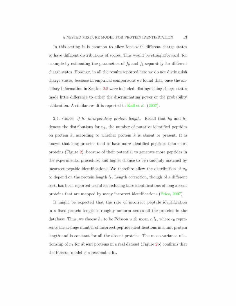
2.4. Choice of h: incorporating protein length. Recall that h0 and h1

denote the distributions for nk, the number of putative identified peptides

on protein k, according to whether protein k is absent or present. It is

known that long proteins tend to have more identified peptides than short

proteins (Figure 2), because of their potential to generate more peptides in

the experimental procedure, and higher chance to be randomly matched by

incorrect peptide identifications. We therefore allow the distribution of nk

to depend on the protein length lk. Length correction, though of a different

sort, has been reported useful for reducing false identifications of long absent

proteins that are mapped by many incorrect identifications (Price, 2007).

It might be expected that the rate of incorrect peptide identification

in a fixed protein length is roughly uniform across all the proteins in the

database. Thus, we choose h0 to be Poisson with mean c0lk, where c0 repre-

sents the average number of incorrect peptide identifications in a unit protein

length and is constant for all the absent proteins. The mean-variance rela-

tionship of nk for absent proteins in a real dataset (Figure 2b) confirms that

the Poisson model is a reasonable fit.


0 500 1000 1500 2000 2500 3000

020

4060

8010

012

0

protein length

num

ber o

f ide

ntifi

ed p

eptid

es

TargetDecoy

0 5 10 15 20 25 30

010

2030

Random

mean of nseq

var o

f nse

q

a b

Fig 2. Number of unique peptide hits and protein length in a yeast data. a. The relation-ship between number of peptide hits (Y-axis) and protein length (X-axis). Red dots aredecoy proteins, which approximate absent proteins; black dots are target proteins, whichcontains both present proteins and absent proteins. b. Verification of the Poisson modelfor absent proteins, approximated by decoy proteins, by mean-variance relationship. Pro-teins are binned by length with each bin containing 1% of data. Mean and variance of thenumber of sequences are calculated for the observations in each bin.

For present proteins, we choose h1 to be Poisson with mean c1lk, where

c1 is a constant that is bigger than c0 to take account of the correct peptide

identifications additional to the incorrect ones. Similar Poisson assumptions,

though with different parameterization, were also made elsewhere (Price,

2007).

Because constructed proteins are assembled from one or more identified

peptides (i.e. nk > 0), we truncate both Poisson distributions at 0, i.e.

(2.11) hj(nk | lk) =exp(−cjlk)(cj lk)

nk

nk!(1 − exp(−cj lk))(nk = 1, 2, . . . ; j = 0, 1).

2.5. Incorporating ancillary information. In addition to the scores on

each peptide identification based on the spectra, other aspects of identi-

fied peptide sequences, such as the number of tryptic termini (NTT) and

the number of missing cleavage (NMC), are informative for the correctness of

peptide identifications (Kall et al., 2007; Keller et al., 2002; Choi and Nesvizhskii,


X

Den

sity

−5 0 5 10

0.0

0.1

0.2

0.3

0.4

NTT

Den

sity

0 1 2

0.0

0.2

0.4

0.6

0.8

1.0

1.2

1.4

NMC

Den

sity

0 1 2

0.0

0.2

0.4

0.6

0.8

a. Summary score X b. Number of tryptic termini c. Number of missing cleavages

Fig 3. The empirical distribution of features from peptide identification in a yeast data.Border histogram: real peptides, which are a mixture of correct and incorrect identifications.Solid histogram: decoy peptides, whose distribution approximates the distribution of theincorrect identifications.

2008a). Because NTT ∈ {0, 1, 2} (Figure 3b), we model it using a multino-

mial distribution. We discretise NMC, which usually ranges from 0 to 10,

into states (0, 1 and 2+) (Figure 3c), and also model it as a multinomial

distribution. These treatments are similar to PeptideProphet.

Peptide identification scores and features on peptide sequences have been

shown to be conditionally independent given the status of peptide identifica-

tion (Keller et al., 2002; Choi and Nesvizhskii, 2008a). Thus we may incor-

porate the ancillary information by replacing fj(Xk,i) in (2.5) and (2.6) with

fj(Xk,i)fNTTj (NTTk,i)f

NMCj (NMCk,i) (j = 0, 1). Further pieces of relevant

information could be incorporated in a similar way.

2.6. Parameter estimation and initialization. We use an expectation-

maximization (EM) algorithm (Dempster et al., 1977) to estimate the pa-

rameters in our model and infer the statuses of peptides and proteins, with

the statuses of proteins (Tk) and peptides (Pk,i) as latent variables. The aug-

mented data for protein k take the form of Yk ≡ (Xk, nk, Tk, Pk,1, . . . , Pk,nk).

The details of the EM algorithm can be found in Appendix A.

To select a reasonable starting point for the EM algorithm, in the real

dataset, we initialize the parameters related to incorrect peptide identifi-


cation (f0, fNTT0 , fNMC

0 and c0) using estimates obtained from the decoy

database (see Section 3.3 for details). For f1, we initialize the shift γ(0) =

mink,i(xk,i)− ǫ, where ǫ is a small positive number to ensure xk,i − γ(0) > 0

for all identified peptides (in both real and decoy databases), and estimate α

and β using the sample mean and sample variance of the scores. We initialize

fNTT1 and fNMC

1 using the peptides that are identified in the real database

and are scored in upper 90% of the identifications to the real database. As

c1 > c0, we choose c1 = bc0, where b is a random number in [1.5, 3]. The

starting values of π∗0 and π1 are chosen randomly from (0, 1). For each infer-

ence, we run the EM algorithm from 10 random starting points and report

the results from the run converging to the highest likelihood.

3. Results.

3.1. Simulation studies. We first use simulation studies to examine the

performance of our approach, and particularly to assess the potential for it to

improve on the types of 2-stage approach used by PeptideProphet and Pro-

teinProphet. Our simulations are based on simulating under models that are

based on our nested mixture model, and ignore many of the complications

of real data (e.g. degeneracy). Thus, their primary goal is not to provide

evidence that our approach is actually superior in practice. Rather the aim

is to provide insight into the kind of gains in performance that might be

achievable in practice, to illustrate settings where the product rule used by

ProteinProphet may perform particularly badly, and to check for robustness

of our method to one of its underlying assumptions (specifically the assump-

tion that the expected proportion of incorrect peptides is the same for all


present proteins). In addition they provide a helpful check on the correctness

of our EM algorithm implementation.

At the peptide level, we compare results from our model with the peptide

probabilities computed by PeptideProphet, and the PeptideProphet proba-

bilities adjusted by ProteinProphet (see section 2.2). At the protein level, we

compare results from our model with three methods: the classical determinis-

tic rule that calls a protein present if it has two or more high-scored peptides

(which we call the “two-peptide rule”), and the two product rules (adjusted

and unadjusted; see section 2.2). Because the product rule is the basis of

ProteinProphet, the comparison with the product rule focuses attention on

the fundamental differences between our method and ProteinProphet, rather

than on the complications of degeneracy handling and other heuristic ad-

justments that are made by the ProteinProphet software.

As PeptideProphet uses Gamma for f0 and Normal for f1, we follow this

practice in the simulations (both for simulating the data, and fitting the

model). In an attempt to generate realistic simulations, we first estimated

parameters from a yeast dataset (Kall et al., 2007) using the model in sec-

tion 2, except for this change of f0 and f1, then simulated proteins from the

estimated parameters (Table 1).

We performed three simulations, S1, S2 and S3, as follows.

S1: This simulation was designed to demonstrate performance when the

data are generated from the same nested mixture model we use for

estimation. Data were simulated from the mixture model, using the

parameters estimated from the real yeast data set considered below.

The resulting data contained 12% present proteins and 88% absent


proteins, where protein length lk ∼ exp(1/500).

S2: Here simulation parameters were chosen to illustrate a scenario where

the product rule performs particularly poorly. Data were simulated as

in S1, except for i) the proportion of present proteins was increased

to 50% (π∗0 = 0.5); ii) the distribution of protein length was modified

so that all present proteins were short (lk ∈ [100, 200]) and absent

proteins were long (lk ∈ [1000, 2000]); and iii) we allowed that absent

proteins may have occasional high-scoring incorrect peptide identifica-

tions (0.2% of peptide scores on absent proteins were drawn from f1

instead of f0).

S3: A simulation to assess sensitivity of our method to deviations from

the assumption that the proportion of incorrect peptides is the same

for all present proteins. Data were simulated as for S1, except π1 ∼

Unif(0, 0.8) independently for each present protein.

In each simulation, 2000 proteins were simulated. We forced all present

proteins to have at least one correctly identified peptide. For simplicity only

one identification score was simulated for each peptide, and the ancillary fea-

tures for all the peptides (NMC=0 and NTT=2) were set identical. We ran

the EM procedure from several random initializations close to the simulation

parameters. We deemed convergence to be achieved when the log-likelihood

increased < 0.001 in an iteration. PeptideProphet (TPP version3.2) and

ProteinProphet (TPP version3.2) were run using their default values.

Parameter estimation

In all the simulations, the parameters estimated from our models are close

to the true parameters (Table 1). Even when absent proteins contain a small


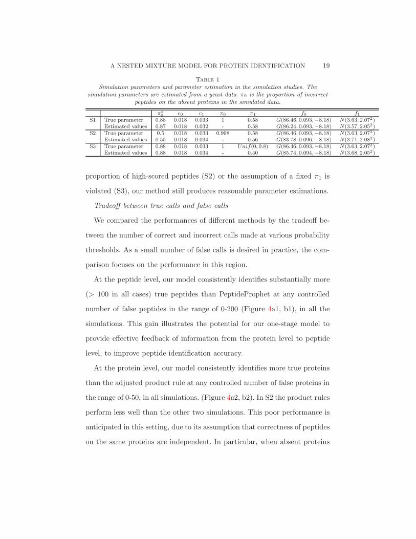
Table 1

Simulation parameters and parameter estimation in the simulation studies. Thesimulation parameters are estimated from a yeast data. π0 is the proportion of incorrect

peptides on the absent proteins in the simulated data.

π∗0

c0 c1 π0 π1 f0 f1

S1 True parameter 0.88 0.018 0.033 1 0.58 G(86.46, 0.093,−8.18) N(3.63, 2.072)Estimated values 0.87 0.018 0.032 - 0.58 G(86.24, 0.093,−8.18) N(3.57, 2.052)

S2 True parameter 0.5 0.018 0.033 0.998 0.58 G(86.46, 0.093,−8.18) N(3.63, 2.072)Estimated values 0.55 0.018 0.034 - 0.56 G(83.78, 0.096,−8.18) N(3.71, 2.082)

S3 True parameter 0.88 0.018 0.033 1 Unif(0, 0.8) G(86.46, 0.093,−8.18) N(3.63, 2.072)Estimated values 0.88 0.018 0.034 - 0.40 G(85.74, 0.094,−8.18) N(3.68, 2.052)

proportion of high-scored peptides (S2) or the assumption of a fixed π1 is

violated (S3), our method still produces reasonable parameter estimations.

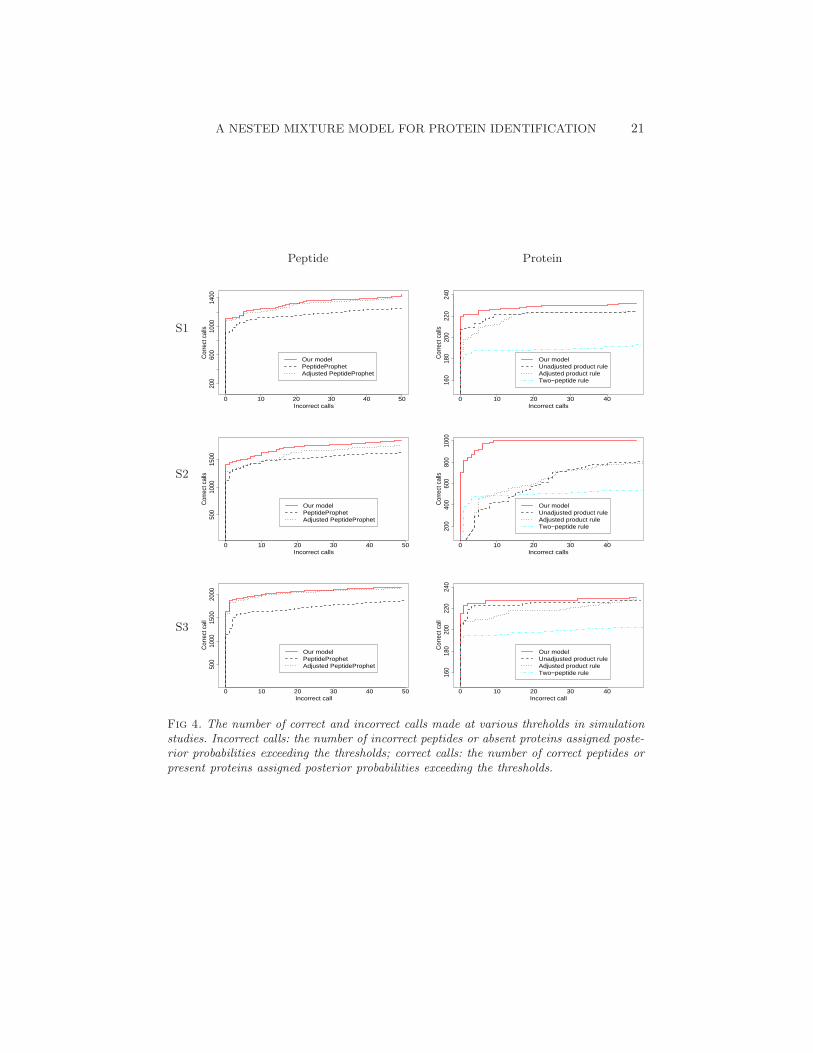
Tradeoff between true calls and false calls

We compared the performances of different methods by the tradeoff be-

tween the number of correct and incorrect calls made at various probability

thresholds. As a small number of false calls is desired in practice, the com-

parison focuses on the performance in this region.

At the peptide level, our model consistently identifies substantially more

(> 100 in all cases) true peptides than PeptideProphet at any controlled

number of false peptides in the range of 0-200 (Figure 4a1, b1), in all the

simulations. This gain illustrates the potential for our one-stage model to

provide effective feedback of information from the protein level to peptide

level, to improve peptide identification accuracy.

At the protein level, our model consistently identifies more true proteins

than the adjusted product rule at any controlled number of false proteins in

the range of 0-50, in all simulations. (Figure 4a2, b2). In S2 the product rules

perform less well than the other two simulations. This poor performance is

anticipated in this setting, due to its assumption that correctness of peptides

on the same proteins are independent. In particular, when absent proteins


with big nk contain a single high-scored incorrect peptide, the product rule

tends to call them present. When present proteins with small nk contain

one or two correct peptides with mediocre scores besides incorrect ones, the

product rule tends to call them absent. The examination of individual cases

confirms that most mistakes made by the product rule belong to either of

the two cases above.

It is interesting that although the adjusted product rule improves peptide

identification accuracy compared with the unadjusted rule, it also worsens

the accuracy of protein identification (at least in S1 and S3). This illustrates

a common pitfall of ad hoc approaches: fixing one problem may unintention-

ally introduce others.

Calibration of probabilities

Methods for identifying proteins and peptides should, ideally, produce ap-

proximately calibrated probabilities, so that the estimated posterior prob-

abilities can be used as a way to assess the uncertainty of the identifica-

tions. In all the three simulations the peptide probabilities from our method

are reasonably well calibrated, whereas the PeptideProphet probabilities are

not, being substantially smaller than the actual probabilities (Figure 5 a).

Our method seems to be better calibrated than the adjusted product rule

at the protein level (Figure 5 b). However, very few proteins are assigned

probabilities ∈ [0.2, 0.9], so larger samples would be needed to confirm this.

3.2. A standard mixture. Mixtures of standard proteins have been used

for assessing the performance of identifications. Although these mixtures

are known to be too simple to reflect the complexity of the realistic samples

and may contain many unknown impurities (Elias et al., 2005), they can


S1

S2

S3

Peptide Protein

0 10 20 30 40 50

200

600

1000

1400

Incorrect calls

Cor

rect

cal

ls

Our modelPeptideProphetAdjusted PeptideProphet

0 10 20 30 40

160

180

200

220

240

Incorrect calls

Cor

rect

cal

ls

Our modelUnadjusted product ruleAdjusted product ruleTwo−peptide rule

0 10 20 30 40 50

500

1000

1500

Incorrect calls

Cor

rect

cal

ls


0 10 20 30 40

200

400

600

800

1000

Incorrect calls

Cor

rect

cal

ls


0 10 20 30 40 50

500

1000

1500

2000

Incorrect call

Cor

rect

cal

l


0 10 20 30 40

160

180

200

220

240

Incorrect call

Cor

rect

cal

l


Fig 4. The number of correct and incorrect calls made at various threholds in simulationstudies. Incorrect calls: the number of incorrect peptides or absent proteins assigned poste-rior probabilities exceeding the thresholds; correct calls: the number of correct peptides orpresent proteins assigned posterior probabilities exceeding the thresholds.


0.0 0.2 0.4 0.6 0.8 1.0

0.0

0.2

0.4

0.6

0.8

1.0

Posterior probability

obse

rved

freq

uenc

y

o

oo

o

oo

o o o o o o o

+++++

+

++

+

+ +

+

+

o+

PeptideProphetOur model

0.0 0.2 0.4 0.6 0.8 1.0

0.0

0.2

0.4

0.6

0.8

1.0

Posterior probability

obse

rved

freq

uenc

y

o

o

o

o

o

o

o o

o

o

+++++

+

+

+

+

+ +

o+

adjusted product ruleOur model

a b

Fig 5. Calibration of posterior probabilities in a simulation study (S1). The observationsare binned by the assigned probabilities. For each bin, the assigned probabilities (X-axis)are compared with the proportion of identifications that are actually correct (Y-axis). (a):peptide probabilities, (b): protein probabilities. Black: PeptideProphet (in (a)) or adjustedproduct rule (in (b)); Red: our method. The size of the points represents the number ofobservations in each bin. Other simulations have similar results

nonetheless be helpful as a way to assess whether a method can effectively

identify the known components.

We applied our method on a standard protein mixture (Purvine et al.,

2004) used in Shen et al. (2008). This dataset consists of the MS/MS spectra

generated from a sample composed of 23 stand-alone peptides and trypsin

digest of 12 proteins. It contains three replicates with a total of 9057 spectra.

The experimental procedures are described in Purvine et al. (2004). We used

Sequest to search, with non-tryptic peptides allowed, a database composed

of the 35 peptides/proteins, typical sample contaminants and the proteins

from Shewanella oneidensis, which are known to be not present in the sam-

ple and serve as negative controls. After matching spectra to peptides, we

obtained 7935 unique putative peptide identifications. We applied our meth-

ods to these putative peptide identifications, and compared results, at both

the protein and peptide levels, with results from the same standard mixture

reported by Shen et al for both their own method (“Hierarchical Statisti-


cal Method”; HSM) and for PeptideProphet/ProteinProphet. Note that in

assessing each method’s performance we make the assumption, standard in

this context, that a protein identification is correct if and only if it involves

a known component of the standard mixture, and a peptide identification is

correct if and only if it involves a peptide whose sequence is a subsequence

of a constituent protein (or is one of the 23 stand-alone peptides).

At the protein level all of the methods we compare here identify all 12

proteins with probabilities close to 1 before identifying any false proteins.

Our method provides a bigger separation between the constituent proteins

and the false proteins, with the highest probability assigned to a false protein

as 0.013 for our method and above 0.8 for ProteinProphet and HSM. At

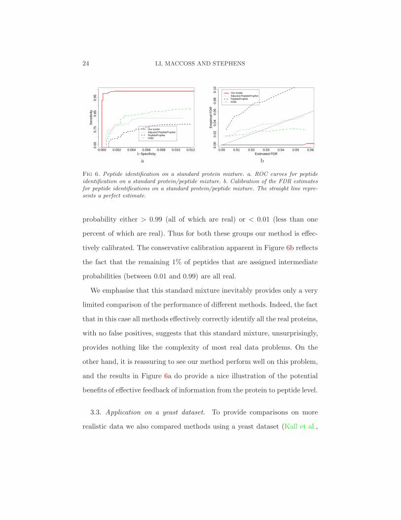
the peptide level, our model shows better discriminating power than all the

other methods (Figure 6a). Again, we ascribe this better performance at the

peptide level to the ability of our model to effectively feedback information

from the protein level to the peptide level.

To assess calibration of the different methods for peptide identification, we

compare the empirical FDR and the estimated FDR (Figure 6a), where the

estimated FDR is computed as the average posterior probabilities to be ab-

sent from the sample for the identifications (Efron et al., 2001; Newton et al.,

2004). None of the methods is particularly well-calibrated for these data:

our method is conservative in its estimated FDR, whereas the other meth-

ods tend to underestimate FDR at low FDRs. Our conservative estimate

of FDR in this case partly reflects the simplicity of this artificial problem.

Indeed, our method effectively separates out the real and not real peptides

almost perfectly in this case: 99% of peptide identifications are assigned


0.000 0.002 0.004 0.006 0.008 0.010 0.012

0.65

0.75

0.85

0.95

1−Specificity

Sen

sitiv

ity

Our modelAdjusted PeptideProphetPeptideProphetHSM

0.00 0.01 0.02 0.03 0.04 0.05 0.06

0.00

0.02

0.04

0.06

0.08

0.10

Estimated FDR

Em

piric

al F

DR

Our modelAdjusted PeptideProphetPeptideProphetHSM

a b

Fig 6. Peptide identification on a standard protein mixture. a. ROC curves for peptideidentification on a standard protein/peptide mixture. b. Calibration of the FDR estimatesfor peptide identifications on a standard protein/peptide mixture. The straight line repre-sents a perfect estimate.

probability either > 0.99 (all of which are real) or < 0.01 (less than one

percent of which are real). Thus for both these groups our method is effec-

tively calibrated. The conservative calibration apparent in Figure 6b reflects

the fact that the remaining 1% of peptides that are assigned intermediate

probabilities (between 0.01 and 0.99) are all real.

We emphasise that this standard mixture inevitably provides only a very

limited comparison of the performance of different methods. Indeed, the fact

that in this case all methods effectively correctly identify all the real proteins,

with no false positives, suggests that this standard mixture, unsurprisingly,

provides nothing like the complexity of most real data problems. On the

other hand, it is reassuring to see our method perform well on this problem,

and the results in Figure 6a do provide a nice illustration of the potential

benefits of effective feedback of information from the protein to peptide level.

3.3. Application on a yeast dataset. To provide comparisons on more

realistic data we also compared methods using a yeast dataset (Kall et al.,


2007). Because the true protein composition of this dataset is unknown,

the comparisons were done by use of a decoy database of artificial proteins,

which is a commonly-used device in this setting (Elias and Gygi, 2007).

Specifically, in the initial step of matching spectra to peptides, each spec-

trum was searched against a combined database, containing both target (i.e.

real) proteins, and decoy (i.e. non-existent) proteins created by permuting

the sequences in the target database. This search was done using Sequest

(Eng, McCormack, and Yates, 1994). The methods are then applied to the

results of this search, and they assign probabilities to both target and de-

coy proteins. Since the decoy proteins cannot be present in the sample,

and assuming that their statistical behaviour is similar to real proteins that

are absent from the sample, a false discovery rate for any given probabil-

ity threshold can be estimated by counting the number of decoy proteins

assigned a probability exceeding the threshold.

The dataset contains 140366 spectra. After matching spectra to peptides

(using Sequest (Eng et al., 1994)), we obtained 116264 unique putative pep-

tide identifications. We used DTASelect (Tabb, McDonald, and Yates, 2002)

to map these peptides back to 12602 distinct proteins (the proteins were

found using DTASelect (Tabb et al., 2002)).

We compared our algorithm with PeptideProphet for peptide inferences

and actual ProteinProphet for protein inferences on this dataset. The HSM

method, whose computational cost and memory requirement are propor-

tional to the factorial of the maximum protein group size, encounters com-

putation difficulties on this dataset and failed to run, because this dataset

contains several large protein groups. We initialized our algorithm using the


approach described in section 2.6, and stopped the EM algorithm when the

change of log-likelihood is smaller than 0.001. PeptideProphet and Protein-

Prophet were run with their default settings.

In this case the comparison is complicated by the presence of peptides

belonging to multiple proteins, i.e. degeneracy, which occurs in about 10%

of proteins in yeast. Unlike our approach, ProteinProphet has routines to

handle degenerate peptides. In brief, it shares each such peptide among

all its corresponding proteins, and estimates an ad hoc weight that each

degenerate peptide contributes to each protein parent. In reporting results,

it groups together proteins with many shared peptide identifications, such as

homologs, and reports a probability for each group (as one minus the product

of the probabilities assigned to each of the individual proteins being absent).

In practice this has the effect of upweighting the probabilities assigned to

large groups containing many proteins.

To make our comparison, we first applied our model ignoring the degener-

acy issue to compute a probability for each protein being present, and then

used these to assign a probability to each group defined by ProteinProphet.

We treated proteins that were not in a group as a group containing one pro-

tein. For our method, we assigned to each group the maximum probability

assigned to any protein in the group. This also has a tendency to upweight

probabilities to large groups, but not by as much as the ProteinProphet

calculation.

Note that the tendency of both methods to upweight probabilities as-

signed to large groups, although a reasonable thing to do, makes reliably

estimating the FDR more difficult. This is because, unlike the real proteins,


the decoy proteins do not fall into homologous groups (i.e. each is in a group

by itself), and so the statistical behaviour of the decoy groups will not exactly

match those of the absent real protein groups. The net effect will be that,

for both methods, the estimates of the FDR based on the decoy comparison

will likely underestimate the true FDR. Further, we suspect that the amount

of underestimation of the FDR will be stronger for ProteinProphet than for

our method, because ProteinProphet more strongly upweights probabilities

assigned to large groups. As a result, comparing the estimated FDRs from

each method, as we do here, may give a slight unfair advantage to Protein-

Prophet. In any case, this rather subtle issue illustrates the severe challenges

of reliably comparing different approaches to this problem.

We assessed the methods by comparing the number of target and decoy

protein groups assigned probabilities exceeding various thresholds. We also

compared the number of decoy and target peptides assigned probabilities

exceeding various thresholds. The results are shown in Figure 7.

At a given number of decoy peptide identifications, our model identified

substantially more target peptides than PeptideProphet (Figure 7 a). Among

these, our method identified most of the target peptides identified by Pep-

tideProphet, in addition to many more not identified by PeptideProphet. For

example, at FDR=0 (i.e. no decoy peptides identified), our method identi-

fied 5362 peptides out of 5394 peptides that PeptideProphet identified, and

additional 3709 peptides that PeptideProphet did not identify.

For the protein idenfication, the methods identified similar numbers of real

protein groups at small FDRs (< 10 decoy proteins identified). At slightly

larger FDRs (> 10 decoy proteins identified) ProteinProphet identified more


0 50 100 150 200

020

0060

0010

000

decoy calls

targ

et c

alls

PeptideProphetour model

0 10 20 30 40

600

800

1000

1200

1400

decoy calls

targ

et c

alls ProteinProphet

Our model

a. Peptide inference b. Protein inference

Fig 7. The number of decoy and target peptides (a) or protein groups (b) assigned prob-abilities exceeding various thresholds in a yeast dataset. Decoy calls: the number of decoypeptides or protein groups assigned a probability exceeding the threshold. Target calls: thenumber of target peptides or protein groups assigned a probability exceeding the threshold.

real protein groups (< 100) than our method. This apparent slightly superior

performance of ProteinProphet may be due, at least in part, to issues noted

above regarding likely underestimation of the FDR in these experiments.

4. Comparison with HSM on another yeast data. To provide

comparisons with HSM method on a realistic dataset, we compared our

method with HSM on another yeast dataset, which was original published

in Elias et al. (2005) and analyzed by Shen et al (Shen et al., 2008). We

were unable to obtain the data from the original publication; instead, we

obtained a processed version from Shen, which produces the results in Shen

et al (Shen et al., 2008). Because the processed data lacks of several key fea-

tures for processing by PeptideProphet and ProteinProphet, we were unable

to compare with PeptideProphet and ProteinProphet on this dataset.

This data set was generated by searching a yeast sample against a se-

quence database composed of 6473 entries of yeast (Saccharomyces cere-

visiae) and 22437 entries of C. elegans (Caenorhabditis elegans). In total,


9272 MS/MS spectra were assigned to 4148 unique peptides. Following Shen

et al (Shen et al., 2008), we exclude 13 charge +1 peptides and fit peptides

with different charge states separately (charge +2: 6869 and charge +3:

2363). The rest of 4135 peptides consists of 3516 yeast peptides and 696

C. elegans peptides. These peptides map to 1011 yeast proteins and 876 C.

elegans proteins. Among all the peptides, 468 (11.3%) are shared by more

than one proteins and 77 peptides are in common between the two species.

Due to peptide sharing between species, 163 C. elegans proteins contain

only peptides that are in common with yeast proteins. These proteins and

peptides shared between species are removed at performance evaluation for

all methods of comparison.

We compare the performance of our method with Shen’s method for both

peptide inferences and protein inferences in Figure 4. Similar to the previ-

ous section, a false discovery rate for any given probability threshold can be

estimated by counting the number of C. elegans proteins assigned a proba-

bility exceeding the threshold, since the C. elegans peptides or proteins that

do not share common sequences with Yeast peptides or proteins cannot be

present in the sample. We assessed the methods by comparing the number

of yeast and C. elegans peptides or proteins assigned probabilities exceeding

various thresholds. The results are shown in Figure 4.

At a given number of C. elegans peptide identifications, our model iden-

tified substantially more yeast peptide identifications than HSM at small

FDR (< 100 C. elegans peptides). For example, at FDR=0, our method

identifies 516 peptides out of 522 peptides that are identified by HSM and

additional 2116 peptides that HSM did not identify. The methods identified


0 50 100 150 200

500

1000

2000

3000

num of C. elegant peptides

num

of Y

east

pep

tides

Our methodHSM

0 10 20 30 40 50

010

020

030

040

050

060

0

num of C.elegant proteins

num

of Y

east

pro

tein

s

Our methodHSM

Peptide Protein

Fig 8. The number of C. elegans and Yeast peptides (a) or proteins (b) assigned probabil-ities exceeding various thresholds in the yeast sample in Shen’s paper.

similar numbers of yeast peptides at higher FDR (> 100 C. elegans pep-

tides). For the protein identification, in the range of FDR that we studied,

our method consistently identifies over 80 more yeast proteins than HSM

at a given number of C. elegans protein identifications, in addition to the

majority (e.g. 96.5% at FDR=0) of the yeast proteins identified by HSM.

Although ProteinProphet results reported by Shen et al (Table 1 in Shen

et al) appear to identify more yeast proteins than our method at a given

number of C. elegans proteins in the range they studied, without access to

the raw data it is difficult to gain insights into the differences. For exam-

ple, the information on whether the reported ProteinProphet identifications

are proteins or protein groups and which proteins are grouped together by

ProteinProphet are unavailable from the data we worked on. However, they

are critical for making comparisons on the same basis. The comparison with

proper handling of these issues (e.g. grouping our protein identifications as

in section 3.3) may lead to conclusions different from naive comparison.


5. Discussion. We have presented a new statistical method for assess-

ing evidence for presence of proteins and constituent peptides identified from

mass spectra. Our approach is, in essence, a model-based clustering method

that simultaneously identifies which proteins are present, and which pep-

tides are correctly identified. We illustrated the potential for this approach

to improve accuracy of protein and peptide identification in both simulated

and real data.

A key feature of our nested mixture model is its ability to incorporate

evidence feedback from proteins to the peptides nested on them. This evi-

dence feedback helps distinguish peptides that are correctly identified but

with weak scores, from those that are incorrectly identified but with higher

scores. The use of a coherent statistical framework also avoids problems

with what we have called the ”product rule”, which is adopted in several

protein identification approaches (Nesvizhskii et al., 2003; Price, 2007), but

is based on an inappropriate assumption of independence of the presence and

absence of different peptides. It has been noted (e.g. (Sadygov et al., 2004;

Feng et al., 2007)) that the product rule tends to wrongly identify as present

long proteins with occasional high-scored incorrect peptides; our simulation

results (Figure 4-2b) illustrate this problem, and demonstrate that our ap-

proach does not misbehave in this way.

In recent work Shen et.al. (Shen et al., 2008) also introduced a nested

latent-variable-based model (HSM) for jointly identifying peptides and pro-

teins from MS/MS data. However, although HSM shares with our model

the goal of simultaneous modeling of peptides and proteins, the structure

of their model is different, and their approach also differs in several details.


Among these differences, the following seem to us most important:

1. HSM accounts for degeneracy, whereas ours does not. We comment

further on this below.

2. HSM includes all the scores for those peptide that match more than

one spectrum, whereas our model uses only the maximum score as a

summary of the evidence. Modeling all scores is obviously preferable

in principle, but in practice it is possible that it could actually de-

crease identification accuracy. We note two particular issues here: a)

Shen et al assume that, conditional on a peptide’s presence/absence

status, multiple scores for the same peptide are independent. This in-

dependence assumption will not hold in practice, and the costs of such

modeling errors could outweigh the benefits of using multiple scores;

b) HSM appears to condition on the number of spectra matched to

each peptide, rather than treating this number as an informative piece

of data. As a result of this conditioning, additional low-scoring hits to

a peptide will always decrease the probability assigned to that pep-

tide. This contrasts with our intuition that additional hits to a peptide

could, in some cases, increase confidence that it is present, even if these

hits have low scores.

3. HSM incorporates only whether the number of hits to peptides in

a protein exceeds some threshold, h (which is set to 1 in their ap-

plications). In contrast our model incorporates the actual number of

(distinct) peptides hitting a protein using a Poisson model. In this way

our model uses more available information, and accounts for variations

in protein length. Note that modeling only whether the number of hits


exceeds h has some undesirable consequences, similar to those noted

above for conditioning on the number of hits to a peptide. For exam-

ple, if h = 1, then a protein that has two hits, each with low scores,

will be assigned a higher identification probability than a protein that

is hit more than twice with low scores.

4. HSM conditions on the number of specific cleavages (NTT in our de-

velopment here) in each putative peptide. Specifically, their parameter

πij(α) is the probability of a particular cleavage event occurring, condi-

tional on NTT. In contrast our model treats the NTT for each peptide

hit as observed data. This may improve identification accuracy be-

cause the distribution of NTT differs greatly for correct and incorrect

identifications (Figure 3).

We expect that some of these differences in detail, perhaps in addition to

other differences not noted here, explain the different performances of our

method and that of Shen et al on the standard mixture data and the yeast

data used in Shen et al (Shen et al., 2008). On the other hand, we agree

with Shen et al that comparisons like these are less definitive, and harder to

interpret, than one would like, because of the absence of good gold-standard

realistic data sets where the truth is known.

We emphasize that, despite its promise, we view the model we present

here as only a starting point towards the development of more accurate

protein and peptide identification software. Not only is the development

of robust fast user-friendly software a considerable task in itself, but there

are also important aspects of real data – specifically degeneracy, which is

prevalent in high-level organisms – that are not properly accounted for by our


model. Currently, most existing approaches to handle degeneracy are based

on heuristics. For example, ProteinProphet groups the proteins with shared

peptides and assigns weights to degenerate peptides using heuristics. An

exception is Shen et al’s model (Shen et al., 2008), which attempts to provide

a coherent statistical solution to the problem by allowing that a peptide

will be present in the digested sample if any one of the proteins containing

that peptide generates it, and assuming that these generation events are

independent (their equation (2)). However, because their model computes

all the possible combinations of protein parents, which increases in the order

of factorials, it is computationally prohibitive to apply their method on data

with moderate or high degree of degeneracy. It should be possible to extend

our model to allow for degeneracy in a similar way. However, there are

some steps that may not be straightforward. For example, we noted above

that our model uses NTT as observed data. But under degeneracy NTT for

each peptide is not directly observed, because it depends on which protein

generated each peptide. Similarly the number of distinct peptides identified

on each protein depends on which protein generated each peptide. While it

should be possible to solve these issues by introducing appropriate latent

variables, some care may be necessary to ensure that, when degeneracy is

accounted for, identification accuracy improves as it should.

Acknowledgement

We thank Dr. Eugene Kolker for providing the standard mixture mass spec-

trometry data, and Jimmy Eng for software support and processing the

standard mixture data.


Appendix A. Here we describe an EM algorithm for the estimation of

Ψ = (π∗0 , π0, π1, µ, σ, α, β, γ, c0 , c1)

T and the protein statuses and the peptide

statuses. To proceed, we use Tk and (Pk,1, . . . , Pk,nk) as latent variables,

then the complete log-likelihood for the augmented data Yk ≡ (Xk, nk, Tk,

Pk,1, . . . , Pk,nk) is

lC(Ψ | Y)

(5.1)

=N

∑

k=1

{

(1 − Tk)[log π∗0 + log h0(nk | lk, nk > 0) +

nk∑

i=1

(1 − Pk,i) log(π0f0(xk,i))+

nk∑

i=1

Pk,i log((1 − π0)f1(xk,i))]

}

+N

∑

k=1

{

Tk[log(1 − π∗0) + log h1(nk | lk, nk > 0) +

nk∑

i=1

(1 − Pk,i) log(π1f0(xk,i))+

nk∑

i=1

Pk,i log((1 − π1)f1(xk,i))]

}

E-step:

Q(Ψ,Ψ(t)) ≡ E(lC(Ψ) | x,Ψ(t))

(5.2)

=N

∑

k=1

P (Tk = 0){log π∗0 + log h0(nk | lk, nk > 0)

+nk∑

i=1

P (Pk,i = 0 | Tk = 0) log(π0f0(xk,i)) +nk∑

i=1

P (Pk,i = 1 | Tk = 0) log((1 − π0)f1(xk,i))}

+N

∑

k=1

P (Tk = 1){log(1 − π∗0) + log h1(nk | lk, nk > 0)

+nk∑

i=1

P (Pk,i = 0 | Tk = 1) log(π1f0(xk,i)) +nk∑

i=1

P (Pk,i = 1 | Tk = 1) log((1 − π1)f1(xk,i))}


Then

T(t)k ≡ E(Tk | xk, nk,Ψ

(t))

(5.3)

=P (Tk = 1,xk, nk | Ψ(t))

P (xk, nk | Ψ(t))

=(1 − π

∗(t)0 )g

(t)1 (xk, nk | Ψ(t))h1(nk)

π∗(t)0 g

(t)0 (xk, nk | Ψ(t))h0(nk) + (1 − π

∗(t)0 )g

(t)1 (xk, nk | Ψ(t))h1(nk)

I(t)0 (Pk,i) ≡ E(Pk,i | Tk = 0, xk,i,Ψ

(t))

(5.4)

=P (Pk,i = 1, xk,i | Tk = 0,Ψ(t))

P (xk,i | Tk = 0,Ψ(t))=

(1 − π(t)0 )f

(t)1 (xk,i)

π(t)0 f

(t)0 (xk,i) + (1 − π

(t)0 )f

(t)1 (xk,i)

(5.5)

I(t)1 (Pk,i) ≡ E(Pk,i | Tk = 1, xk,i,Ψ

(t)) =(1 − π

(t)1 )f

(t)1 (xk,i)

π(t)1 f

(t)0 (xk,i) + (1 − π

(t)1 )f

(t)1 (xk,i)

M-step:

Now we need maximize Q(Ψ,Ψ(t)). Since the mixing proportions and the

distribution parameters can be factorized into independent terms, we can

optimize them separately. The MLE of the mixing proportion π∗0 is:

(5.6) π∗(t+1)0 =

∑Nk=1(1 − T

(t)k )

N

(5.7) π(t+1)0 =

∑Nk=1[(1 − T

(t)k )

∑nk

i=1(1 − I(t)0 (Pk,i))]

∑Nk=1(1 − T

(t)k )nk

(5.8) π(t+1)1 =

∑Nk=1[T

(t)k

∑nk

i=1(1 − I(t)1 (Pk,i))]

∑Nk=1 T

(t)k nk


If incorporating ancillary features of peptides, we replace fj(xki) with

fj(xki)fnmc

j (nmck,i)fnttj (nttk,i) as in Section 2.5, where xki

is the identi-

fication score, nmck,i is the number of missed cleavage and nttk,i is the

number of tryptic termini (with values s = 0, 1, 2). As described in Section

2.3, f0 = N(µ, σ2) and f1 = Gamma(α, β, γ). We can obtain closed form

estimators for f0 as follows, and estimate f1 using the numerical optimizer

optimize() in R.

(5.9) µ =

∑Nk=1

∑nk

i=1

[

(1 − T(t)k )(1 − I

(t)0 (Pk,i)) + T

(t)k (1 − I

(t)1 (Pk,i))

]

xki

∑Nk=1

∑nk

i=1

[

(1 − T(t)k )(1 − I

(t)0 (Pk,i)) + T

(t)k (1 − I

(t)1 (Pk,i))

]

(5.10)

σ2 =

∑Nk=1

∑nk

i=1

[

(1 − T(t)k )(1 − I

(t)0 (Pk,i)) + T

(t)k (1 − I

(t)1 (Pk,i))

]

(xki− µ0)

2

∑Nk=1

∑nk

i=1

[

(1 − T(t)k )(1 − I

(t)0 (Pk,i)) + T

(t)k (1 − I

(t)1 (Pk,i))

]

As described in Section 2.5, we discretise NMC, which usually ranges from

0 to 10, into states s = 0, 1, 2, with s = 2 representing all values ≥ 2. So the

MLE of fnmc0 is:

(5.11) fnmc0 (nmck,i) =

w(t)s

∑2s=0 w

(t)s

where

(5.12)

w(t)s =

N∑

k=1

nk∑

i=1

(1−T(t)k )(1−I

(t)0 (Pk,i))1(nmck,i = s)+

N∑

k=1

nk∑

i=1

T(t)k (1−I

(t)1 (Pk,i))1(nmck,i = s)

Similarly, the MLE of fnmc1 is:

(5.13) fnmc1 (nmck,i) =

v(t)s

∑2s=0 v

(t)s


where

(5.14)

v(t)s =

N∑

k=1

nk∑

i=1

(1−T(t)k )I

(t)0 (Pk,i)1(nmck,i = s)+

N∑

k=1

nk∑

i=1

T(t)k I

(t)1 (Pk,i)1(nmck,i = s)

The MLE of fnttj takes the similar form as fnmc

j , j=0,1, with states s =

0, 1, 2.

For h0 and h1, the terms related to h0 and h1 in Q(Ψ,Ψt) are:

(5.15)N

∑

k=1

(1 − Tk) log h0(nk) =N

∑

k=1

(1 − Tk) logexp(−c0lk)(c0lk)

nk

nk!(1 − exp(−c0lk))

(5.16)N

∑

k=1

Tk log h1(nk) =N

∑

k=1

Tk logexp(−c1lk)(c1lk)

nk

nk!(1 − exp(−c1lk))

The MLE of the above does not have close form, so we estimate them using

optimize() in R.

References.

Blei, D., T. Gri, M. Jordan, and J. Tenenbaum (2004). Hierarchical topic models and the

nested chinese restaurant process. In NIPS.

Choi, H. and A. I. Nesvizhskii (2008a). Semisupervised model-based validation of peptide

identifications in mass spectrometry-based proteomics. J. Proteome Res. 7, 254–265.

Choi, H. and A. I. Nesvizhskii (2008b). Semisupervised model-based validation of peptide

identifications in mass spectrometry-based proteomics. J. Proteome Res. 7, 254–265.

Coon, J. J., J. E. Syka, J. Shabanowitz, and D. Hunt (2005). Tandem mass spectrometry

for peptide and proteins sequence analysis. BioTechniques 38, 519–521.

Dempster, A., N. Laird, and D. Rubin (1977). Maximum likelihood from incomplete data

via the em algorithm. J. R. Statist. Soc. B 39 (1), 1–38.

Efron, B., R. Tibshirani, J. D. Storey, and V. G. Tusher (2001). Empirical bayes analysis

of a microarray experiment. Journal of the American Statistical Association 96, 1151–

1160.


Elias, J., B. Faherty, and S. Gygi (2005). Comparative evaluation of mass spectrometry

platforms used in large-scale proteomics inverstigations. Nature Methods 2, 667–675.

Elias, J. and S. Gygi (2007). Target-decoy search strategy for increased confidence in

large-scale protein identifications by mass spectrometry. Nature Methods 4, 207–214.

Eng, J., A. McCormack, and J. I. Yates (1994). An approach to correlate tandem mass

spectral data of peptides with amino acid sequences in a protein database. J. Am. Soc.

Mass Spectrom 5, 976–989.

Feng, J., Q. Naiman, and B. Cooper (2007). Probability model for assessing protein assem-

bled from peptide sequences inferred from tandem mass spectrometry data. Analytical

Chemistry 79, 3901–3911.

Kall, L., J. Canterbury, J. Weston, and M. J. Noble, W. S.and MacCoss (2007). A

semi-supervised machine learning technique for peptide identification from shotgun pro-

teomics datasets. Nature Methods 4, 923–925.

Keller, A. (2002). Experimental protein mixture for validating tandem mass spectral

analysis. Omics 6, 207–12.

Keller, A., A. Nesvizhskii, E. Kolker, and R. Aebersold (2002). Empirical statistical model

to estimate the accuracy of peptide identifications made by ms/ms and database search.

Anal. Chem. 74, 5383–5392.

Kinter, M. and N. E. Sherman (2003). Protein sequencing and identification using tandem

mass spectrometry. Wiley.

Li, Q. (2008). Statistical methods for peptide and protein identification in mass spectrom-

etry. Ph. D. thesis, University of Washington, Seattle, WA.

Nesvizhskii, A., A. Keller, E. Kolker, and R. Aebersold (2003). A statistical model for

identifying proteins by tandem mass spectrometry. Anal. Chem. 75, 4646–4653.

Nesvizhskii, A. I. and R. Aebersold (2004). Analysis, statistical validation and disser-

mination of large-scale proteomics datasets generated by tandem ms. Drug Discovery

Todays 9, 173–181.

Newton, M. A., A. Noueiry, D. Sarkar, and P. Ahlquist (2004). Detecting differential

gene expression with a semiparameteric hierarchical mixture method. Biostatistics 5,

155–176.

Price, T. e. a. (2007). Ebp, a program for protein identification using multiple tandem


mass spectrometry data sets. Mol. Cell. Proteomics 6, 537–536.

Purvine, S., A. F. Picone, and E. Kolker (2004). Standard mixtures for proteome studies.

Omics 8, 79–92.

Sadygov, R., H. Liu, and J. Yates (2004). Statistical models for protein validation using

tandem mass spectral data and protein amino acid sequence databases. Anal Chem 76,

1664–1671.

Sadygov, R. and J. Yates (2003). A hypergeometric probability model for protein identifi-

cation and validation using tandem mass spectral data and protein sequence databases.

Anal. Chem. 75, 3792–3798.

Schwarz, G. (1978). Estimating the dimension of a model. Annals of Statistics 6, 461–464.

Shen, C., Z. Wang, G. Shankar, X. Zhang, and L. Li (2008). A hierarchical statistical

model to assess the confidence of peptides and proteins inferred from tandem mass

spectrometry. Bioinformatics 24, 202–208.

Steen, H. and M. Mann (2004). The abc’s (and xyz’s) of peptide sequencing. Nature

Reviews 5, 699–712.

Tabb, D., H. McDonald, and J. I. Yates (2002). Dtaselect and contrast: tools for assembling

and comparing protein identifications from shotgun proteomics. J. Proteome Res. 1,

21–36.

Vermunt, J. K. (2003). Multilevel latent class models. Sociological Methodology 33, 213–

239.

Department of Statistics

University of Washington

Box 354322

Seattle, WA 98195-4322, USA

E-mail: [email protected]

Department of Genome Sciences

University of Washington

Box 355065

Seattle, WA 98195-5065, USA


Department of Statistics and Human Genetics

University of Chicago

Eckhart Hall Room 126

5734 S. University Avenue

Chicago, IL 60637, USA


mailto:[email protected]



a nested mixture model for protein identification...

Documents