a natural computation approach to biology
TRANSCRIPT

PhD Dissertation
International Doctorate School in Information andCommunication Technologies
DIT - University of Trento
A Natural Computation Approach To
Biology
Modelling Cellular Processes and Populations of
Cells With Stochastic Models of P Systems
Sean Sedwards
Advisor:
Prof. Corrado Priami
Universita degli Studi di Trento
Co-Advisor:
Dr. Matteo Cavaliere
The Microsoft Research – University of Trento
Centre for Computational and Systems Biology
February 2009

The Microsoft Research – University of Trento
Centre for Computational and Systems Biology

Abstract
According to the well-accepted paradigm, the underlying constituents of bi-
ology are discrete molecules, with some being in very small copy numbers.
It is therefore most precise to model the interaction of biological substances
as discrete events connecting discrete states. Using this abstraction it is
then natural to treat molecular interactions as being part of a computation
and to perform formal analysis on them using the techniques of computer
science. In this way it is possible to extract useful information about bio-
logical systems in an automatic way.
Membranes and membrane proteins are fundamental to the operation of
biological cells, hence this thesis presents three new computational models
designed to represent biological systems, based on models of membrane com-
puting: Membrane Systems with Peripheral Proteins (MSPP), Membrane
Systems with Peripheral and Integral Proteins (MSPIP) and Colonies of
Synchronizing Agents (CSA). MSP(I)P is close to biologists’ prevailing
view of the cell and hence is highly compatible with existing biochemical
models. CSA is an hierarchical paradigm designed to represent complex
systems such as populations of cells and tissues. This work extends the
corpus of knowledge about biology and the theory of computation by prov-
ing technical results related to these models.
The MSPP, MSPIP and CSA models have associated software imple-
mentations which allow the simulation of the temporal evolution of biologi-
cal models by means of multiset rewriting under the control of a stochastic
algorithm. One of these, Cyto-Sim (implementing the MSPP and MSPIP
models), being most developed, is presented in detail with several examples.

Stochastic simulation is inherently computationally intensive and hier-
archical systems particularly so. This thesis presents a new state of the art
stochastic simulation algorithm for hierarchical and agent-based systems
(the Method of Partial Propensities) and uses this result to improve the
state of the art of stochastic simulation algorithms for well stirred chemical
systems (the Method of Arbitrary Partial Propensities).
The noise evident in stochastic simulations is a potentially useful char-
acteristic, containing information about the system being simulated. To
extract detailed measures of stochasticity and the behaviour of a system,
a new technique using Fourier analysis is presented and illustrated. With
this it is possible to create a space of phenotype to characterise models and
the performance of simulation algorithms.
Keywords
[Natural Computing, Stochastic Simulation, Multiset Re-writing, Systems
Biology, Biological Modelling, Agents, P Systems, Membranes, Fourier
Analysis]

Contents
1 Introduction 1
1.1 The Context . . . . . . . . . . . . . . . . . . . . . . . . . . 1
1.2 The Problem . . . . . . . . . . . . . . . . . . . . . . . . . 2
1.3 The Solution . . . . . . . . . . . . . . . . . . . . . . . . . 3
1.4 Innovative Aspects . . . . . . . . . . . . . . . . . . . . . . 4
1.5 Structure of the Thesis . . . . . . . . . . . . . . . . . . . . 6
1.6 Publications relating to the chapters presented in this thesis 7
2 Preliminaries 9
2.1 Membrane Systems . . . . . . . . . . . . . . . . . . . . . . 17
2.1.1 Membrane syntax . . . . . . . . . . . . . . . . . . . 19
3 Membrane Systems with Peripheral Proteins 23
3.1 Introduction and motivations . . . . . . . . . . . . . . . . 24
3.2 Membrane Operations with Peripheral Proteins . . . . . . 26
3.3 Membrane Systems with Peripheral Proteins . . . . . . . . 29
3.4 Evolution of the System . . . . . . . . . . . . . . . . . . . 30
3.5 Reachability with Free-Parallel Evolution . . . . . . . . . . 32
3.6 Reachability with Maximal-Parallel Evolution . . . . . . . 38
3.7 Conclusions and Open Problems . . . . . . . . . . . . . . . 51
4 Membrane Systems with Peripheral & Integral Proteins 53
i

4.1 Introduction . . . . . . . . . . . . . . . . . . . . . . . . . . 54
4.2 Operations with Peripheral and Integral Proteins . . . . . 56
4.2.1 Operations . . . . . . . . . . . . . . . . . . . . . . . 57
4.3 Membrane Systems with Peripheral and Integral Proteins . 60
4.4 Modelling and Simulation of Cellular Processes . . . . . . 63
4.4.1 The Stochastic Algorithm . . . . . . . . . . . . . . 63
4.4.2 Modelling a Noise-Resistant Circadian Oscillator . . 64
4.4.3 Modelling Saccharomyces Cerevisiae Mating Response 67
4.5 Perspectives . . . . . . . . . . . . . . . . . . . . . . . . . . 68
5 Cyto-Sim 75
5.1 Introduction . . . . . . . . . . . . . . . . . . . . . . . . . . 76
5.2 Approach . . . . . . . . . . . . . . . . . . . . . . . . . . . 77
5.3 Methods . . . . . . . . . . . . . . . . . . . . . . . . . . . . 78
5.4 Discussion . . . . . . . . . . . . . . . . . . . . . . . . . . . 79
5.5 The Cyto-Sim language . . . . . . . . . . . . . . . . . . . . 80
5.5.1 Comments . . . . . . . . . . . . . . . . . . . . . . . 81
5.5.2 Constant Declaration . . . . . . . . . . . . . . . . . 82
5.5.3 Object Declaration . . . . . . . . . . . . . . . . . . 82
5.5.4 Rule Definition . . . . . . . . . . . . . . . . . . . . 82
5.5.5 Petri Net Definition . . . . . . . . . . . . . . . . . . 84
5.5.6 Compartment Definition . . . . . . . . . . . . . . . 85
5.5.7 System Statement . . . . . . . . . . . . . . . . . . . 86
5.5.8 Evolve Statement . . . . . . . . . . . . . . . . . . . 87
5.5.9 Plot Statement . . . . . . . . . . . . . . . . . . . . 88
5.6 Extended syntax . . . . . . . . . . . . . . . . . . . . . . . 89
5.7 Examples . . . . . . . . . . . . . . . . . . . . . . . . . . . 92
5.7.1 Lotka-Volterra Reactions . . . . . . . . . . . . . . . 92
5.7.2 Oregonator . . . . . . . . . . . . . . . . . . . . . . 92
ii

5.7.3 Noise-Resistant Oscillator . . . . . . . . . . . . . . 93
5.7.4 Oscillatory behaviour of NF-κB . . . . . . . . . . . 94
5.7.5 Stable and unstable attractors . . . . . . . . . . . . 104
6 Colonies of Synchronizing Agents 111
6.1 Introduction and motivations . . . . . . . . . . . . . . . . 112
6.2 Preliminaries . . . . . . . . . . . . . . . . . . . . . . . . . 115
6.3 Colonies of Synchronizing Agents . . . . . . . . . . . . . . 122
6.4 Computational Power of CSAs . . . . . . . . . . . . . . . . 128
6.5 Robustness of CSAs: A Formal Study . . . . . . . . . . . . 141
6.6 A Computational Tree Logic for CSAs . . . . . . . . . . . 152
6.7 Prospects . . . . . . . . . . . . . . . . . . . . . . . . . . . 158
7 Stochastic Simulation Algorithms 161
7.1 Stochastic Simulation . . . . . . . . . . . . . . . . . . . . . 161
7.2 Markov processes . . . . . . . . . . . . . . . . . . . . . . . 163
7.3 Hierarchy of simulation methods . . . . . . . . . . . . . . . 165
7.3.1 Exact methods . . . . . . . . . . . . . . . . . . . . 166
7.3.2 The Next Reaction Method . . . . . . . . . . . . . 170
7.3.3 Approximate methods . . . . . . . . . . . . . . . . 172
7.3.4 Numerical precision . . . . . . . . . . . . . . . . . . 177
8 The Method of Partial Propensities 181
8.1 Introduction . . . . . . . . . . . . . . . . . . . . . . . . . . 182
8.2 The Direct Method . . . . . . . . . . . . . . . . . . . . . . 184
8.2.1 Computational complexity of the DM . . . . . . . . 185
8.2.2 Optimizations of the DM . . . . . . . . . . . . . . . 186
8.3 The Method of Partial Propensities . . . . . . . . . . . . . 187
8.3.1 Computational complexity of CSAs using the DM . 189
8.3.2 Details of the Method of Partial Propensities . . . . 192
iii

8.4 Results . . . . . . . . . . . . . . . . . . . . . . . . . . . . . 195
8.5 Discussion . . . . . . . . . . . . . . . . . . . . . . . . . . . 198
8.6 Conclusion . . . . . . . . . . . . . . . . . . . . . . . . . . . 200
9 The Method of Arbitrary Partial Propensities 203
9.1 Introduction and motivation . . . . . . . . . . . . . . . . . 204
9.2 Computational cost of exact stochastic simulation algorithms 205
9.2.1 The First Reaction Method . . . . . . . . . . . . . 206
9.2.2 The Direct Method . . . . . . . . . . . . . . . . . . 206
9.2.3 The Next Reaction Method . . . . . . . . . . . . . 206
9.2.4 The Optimized Direct Method . . . . . . . . . . . . 208
9.3 Optimizations . . . . . . . . . . . . . . . . . . . . . . . . . 212
9.3.1 Optimization 1 . . . . . . . . . . . . . . . . . . . . 212
9.3.2 Optimization 2 . . . . . . . . . . . . . . . . . . . . 214
9.3.3 Optimization 3 . . . . . . . . . . . . . . . . . . . . 215
9.4 The Method of Arbitrary Partial Propensities . . . . . . . 215
9.4.1 Details of the MAPP . . . . . . . . . . . . . . . . . 216
9.4.2 Comparison of the MAPP, NRM and ODM . . . . 218
9.4.3 Generalization of the MAPP . . . . . . . . . . . . . 220
9.5 Results . . . . . . . . . . . . . . . . . . . . . . . . . . . . . 221
9.6 Conclusion . . . . . . . . . . . . . . . . . . . . . . . . . . . 228
10 Fourier analysis of stochastic simulations 231
10.1 Average behaviour . . . . . . . . . . . . . . . . . . . . . . 232
10.2 The Fourier transform . . . . . . . . . . . . . . . . . . . . 233
10.3 Computational cost . . . . . . . . . . . . . . . . . . . . . . 237
10.4 Statistical measures over DFT spectra . . . . . . . . . . . 238
10.4.1 Statistical measures . . . . . . . . . . . . . . . . . . 242
10.5 Fourier analysis of budding yeast mutants . . . . . . . . . 243
10.6 Prospects . . . . . . . . . . . . . . . . . . . . . . . . . . . 245
iv

11 Conclusions 251
11.1 Prospects and open problems . . . . . . . . . . . . . . . . 256
v

List of Tables
5.1 Timings of Cyto-Sim and other popular simulators. . . . . 80
7.1 Computational operations considered to be O(1). . . . . . 168
vii


List of Figures
2.1 Diagrammatic representation of a P System (Membrane Sys-
tem) showing typical features. . . . . . . . . . . . . . . . . 18
4.1 Endocytosis of LDL. . . . . . . . . . . . . . . . . . . . . . 54
4.2 Graphical representation of a membrane system. . . . . . . 57
4.3 Examples of attachin, attachout, de − attachin and de −attachout rules. . . . . . . . . . . . . . . . . . . . . . . . . 59
4.4 Example of an evol rule. . . . . . . . . . . . . . . . . . . . 60
4.5 Reaction scheme and simulation results of noise-resistant
oscillator. . . . . . . . . . . . . . . . . . . . . . . . . . . . 66
4.6 A Ppi system model of the noise resistant oscillator. . . . . 72
4.7 Simulated effect of switching off a gene in the noise-resistant
oscillator. . . . . . . . . . . . . . . . . . . . . . . . . . . . 73
4.8 Model and simulation results of Saccharomyces cerevisiae
mating response. . . . . . . . . . . . . . . . . . . . . . . . 73
4.9 Ppi system model of G-protein cycle and corresponding sim-
ulator script. . . . . . . . . . . . . . . . . . . . . . . . . . 74
5.1 Phase plot of the Lotka-Volterra model. . . . . . . . . . . . 89
5.2 Lotka-Volterra reactions using Cyto-Sim native rule syntax. 94
5.3 Petri net representation of Lotka-Volterra reactions. . . . . 94
5.4 Lotka-Volterra reactions using a Petri net incidence matrix. 95
5.5 Typical simulation trace of Lotka-Volterra reactions. . . . . 95
ix

5.6 Oregonator oscillator modelled using Cyto-Sim native rule
syntax. . . . . . . . . . . . . . . . . . . . . . . . . . . . . . 96
5.7 Petri net representation of Oregonator oscillator. . . . . . . 96
5.8 Oregonator oscillator modelled using a Petri net incidence
matrix. . . . . . . . . . . . . . . . . . . . . . . . . . . . . . 97
5.9 Typical simulation trace of Oregonator oscillator. . . . . . 97
5.10 Reaction scheme of noise-resistant oscillator. . . . . . . . . 98
5.11 Noise-resistant oscillator modelled using Cyto-Sim native re-
action rules. . . . . . . . . . . . . . . . . . . . . . . . . . . 99
5.12 Petri net representation of the noise-resistant oscillator. . . 100
5.13 Noise-resistant oscillator modelled using a Petri net inci-
dence matrix. . . . . . . . . . . . . . . . . . . . . . . . . . 101
5.14 Typical single simulation trace of the noise-resistant oscillator.102
5.15 Typical simulation trace of switching off a gene in the noise-
resistant oscillator. . . . . . . . . . . . . . . . . . . . . . . 102
5.16 Model demonstrating oscillatory behaviour in NF-κB. . . . 102
5.17 Reaction dependency of NF-κB model. . . . . . . . . . . . 105
5.18 Typical simulation results for NF-κB model. . . . . . . . . 106
5.19 Cyto-Sim script to demonstrate stable and unstable attractors.108
5.20 Cyto-Sim simulation traces showing how initial conditions
tend to stable attractors. . . . . . . . . . . . . . . . . . . . 109
5.21 Budding yeast cell cycle model of [82] expressed in Cyto-Sim
extended syntax. . . . . . . . . . . . . . . . . . . . . . . . 110
6.1 Application of an instance of an evolution rule. . . . . . . 127
6.2 Application of an instance of a synchronization rule. . . . . 127
6.3 Alternative maximally-parallel and asynchronous evolutions
of a CSA. . . . . . . . . . . . . . . . . . . . . . . . . . . . 129
6.4 Two possible asynchronous computations of a CSA. . . . . 143
x

6.5 Robust behaviour of a CSA despite removal of an agent. . 144
6.6 Lack of robustness when an agent is removed from a CSA. 144
7.1 Diagram showing the relation of various simulation methods
based on the Markovian assumption. . . . . . . . . . . . . 166
7.2 Selection of a reaction using the Direct Method. . . . . . . 169
7.3 Reaction dependencies of the noise-resistant oscillator model. 173
8.1 Algorithm scaling with increasing numbers of agents. . . . 198
9.1 Relative reaction frequency in the simulation of the model
of NF-κB oscillation. . . . . . . . . . . . . . . . . . . . . . 210
9.2 Relative reaction frequency in the simulation of the noise-
resistant oscillator. . . . . . . . . . . . . . . . . . . . . . . 211
9.3 The two layer data structure used by the MAPP for the case
of 11 reaction. . . . . . . . . . . . . . . . . . . . . . . . . . 217
9.4 The reaction frequency distribution of three instances of the
noise resistant oscillator. . . . . . . . . . . . . . . . . . . . 224
9.5 Algorithm scaling with increasing numbers of parallel reac-
tions having average dependency 1. . . . . . . . . . . . . . 225
9.6 Algorithm scaling with increasing numbers of reactions, based
on multiple parallel instances of the noise resistant oscillator. 226
9.7 Algorithm scaling with increasing numbers of reactions, based
on multiple parallel instances of the NF-κB model. . . . . 227
10.1 Averaged stochastic time series of the noise resistant oscillator.233
10.2 Distributions of amounts of two proteins of the noise resis-
tant oscillator. . . . . . . . . . . . . . . . . . . . . . . . . . 234
10.3 Time and frequency domain representations of x(t) = sin(2πt)+
sin(4πt) . . . . . . . . . . . . . . . . . . . . . . . . . . . . 235
xi
10.4 Time and frequency domain representations of function with
added uncorrelated Gaussian noise. . . . . . . . . . . . . . 237
10.5 Convergence of statistical measures relating to stochastic
simulations of the budding yeast cell cycle. . . . . . . . . . 239
10.6 Comparison of DFT spectra of stochastic and deterministic
simulations. . . . . . . . . . . . . . . . . . . . . . . . . . . 241
10.7 DFT spectra and associated statistical measures of NF-κBn
oscillation. . . . . . . . . . . . . . . . . . . . . . . . . . . . 244
10.8 The simplified generic model of budding yeast cell cycle. . 245
10.9 Typical deterministic time series of concentrations for the
simplified budding yeast cell cycle. . . . . . . . . . . . . . 246
10.10Typical stochastic simulation traces of the simplified bud-
ding yeast cell cycle. . . . . . . . . . . . . . . . . . . . . . 246
10.11Typical DFT distributions for wild type budding yeast. . . 247
10.12Typical DFT distributions for sic1∆ yeast mutant. . . . . 248
10.13Typical DFT distributions for cln1∆, cln2∆, cln3∆, sic1∆
yeast mutant. . . . . . . . . . . . . . . . . . . . . . . . . . 248
10.14Typical DFT distributions for cdh1∆ yeast mutant. . . . . 249
10.15Total measures of viability for wild type and three mutant
yeast strains. . . . . . . . . . . . . . . . . . . . . . . . . . 249
xii

Chapter 1
Introduction
1.1 The Context
The sequencing of the human genome is a well known and successful appli-
cation of information technology to biology. Moreover, the information so
derived is being successfully interrogated and manipulated using compu-
tational techniques. This apparent success and the continuing exponential
growth in computational power (i.e., Moore’s law) leads scientists to believe
that computers may be successfully applied to other areas of biology [43].
It is expected that cells, tissues and even entire organisms may be accu-
rately simulated by computational models, in order to accelerate biological
research and so aid disease prevention and cure.
Large amounts of biological data are available from high throughput
experimental techniques and the emerging field of Systems Biology thus
requires predictive and informative models to make sense of it. Such models
need to be intuitive and efficient in execution in order to minimise the
apparent and real computational complexities. Much of the data gathered
so far has been done in a piecemeal and informal way, being driven by the
availability of technology. In order to gain inference from the data, it is
necessary for models to be described in a structured way which may be
formally analysed.
1

1.2 Introduction
Natural computing is a field of computer science which derives inspira-
tion for new computational paradigms from biology; Nature having evolved
efficient ways to solve difficult problems. Turning this process around; hav-
ing extracted the key elements of Nature’s solution to form a formal frame-
work, it is then conceivable to re-categorise natural models in a formal way
and thus gain insight about how they work. This is one of the essential
premises of this thesis.
1.2 The Problem
The reasonable expectation to use the power of computers to understand
biology may be hampered by the inherent difference between having a
static description of the biology (e.g., a genome or pathway) versus the
dynamic system it describes. In computational terms, this is analogous to
the difference between the description of a program versus the behaviour
of the resulting process when the program is executed. It was hoped that
knowing all the genes of an organism would allow its complete characteri-
sation, however it seems that there are epigenomic and other effects which
result in significant phenotypic differences. While it is not unreasonable to
suppose that an organism’s genes act to regulate its behaviour, it seems
that precise prediction of future behaviour will depend critically on equally
precise knowledge of its history. From this it becomes clear that analysis
of the dynamics of biological models will be crucial and that simulation of
such models in time will play an important role.
Molecular biology has been successfully modelled by the traditional tools
of dynamical systems: differential equations. These accurately describe the
interactions of molecular populations as flows when the number of similar
discrete interaction events is sufficiently large for a continuous approxima-
tion to be valid. As the precision of biological measurements and experi-
2
Introduction 1.3
ments increases, however, it has become clear that some critical molecules
are in very low copy number (single genes being an obvious example [28])
and that there are a great many different interactions. Under these con-
ditions, differential equations can only describe an average behaviour, at
best, and models using them tend to become unwieldy and inefficient. The
paradigm of discrete molecules and discrete transitions, which in the ther-
modynamic limit makes differential equations plausible, more directly leads
to the possibility to construct transition systems which may be analysed
by the techniques of computer science formal methods.
1.3 The Solution
Starting from the premise of modelling biology using a computational
paradigm, this work builds on one such that is inspired by biological cells
and tissues: P Systems (a.k.a. Membrane Systems). The original purpose
of the paradigm was to explore the computational power of computing
devices having a cellular structure and using computational operations in-
spired by chemical reactions and the passage of molecules between cells. In
order to more easily model the diversity of biology, however, it is necessary
to extend the basic concept of a Membrane System to include specific bio-
logical features. Having done so, it is necessary to provide proofs of various
properties of the extended models and to facilitate their simulation with
software implementations. A further critical requirement is the analysis of
the results of using such simulators.
This thesis presents two new classes of models of Membrane Systems,
tailored to represent ‘well-stirred’ and hierarchical biochemical systems.
The underlying formalism is intuitive to non-experts and has a wealth of
existing technical results for reference as well as active ongoing research.
Several results are presented here which extend the corpus and aid the
3
1.4 Introduction
understanding of biological computations. Since discrete and stochastic
formalisms which model individual molecular interactions potentially give
the most accurate dynamical representation of biological systems, the im-
plementations of these models employ the concept of multiset rewriting
controlled by a stochastic simulation algorithm. Two simulators and their
associated languages have been created, one of which (Cyto-Sim) is pre-
sented in detail. To ameliorate the computational complexity of stochastic
simulation two new state of the art simulation algorithms have been de-
veloped and are presented here. Finally, a new technique based on Fourier
analysis is presented which extracts useful information from stochastic sim-
ulations.
1.4 Innovative Aspects
The specific innovative aspects relating to this thesis are listed below. The
current author’s original publications from which these innovations are
drawn are listed in Section 1.6.
• Membrane Systems with Peripheral Proteins: A new model
of membrane systems featuring objects attached to both inner and
outer surfaces of a membrane. This model more accurately represents
biological reality than previously considered models. Several technical
results are presented which help to clarify the way biological processes
work.
• Membrane Systems with Peripheral and Integral Proteins:
An extension of the peripheral protein model to include integral pro-
teins, further enhancing the model’s biological plausibility by allowing
known biological entities to be represented explicitly.
• Cyto-Sim: A software implementation of the two presented mem-
4

Introduction 1.5
brane systems models uses an efficient stochastic simulator, intuitive
textual modelling language and provides various graphical and statis-
tical outputs. Other features related to abstraction and compatibility
with other formalisms include:
⊲ Interconversion of native modelling language to various versions
of SBML.
⊲ Extension of native modelling language to represent models as
Petri nets.
⊲ Export of native models to ordinary differential equations (ODEs)
in MATLAB m-file format.
⊲ Extension of modelling language and simulator to accept arbitrary
kinetic functions, as used by many existing biological models, thus
facilitating an additional level of abstraction.
• Colonies of Synchronizing Agents: A new, ‘elegant’, agent-based
paradigm that generalises and extends earlier models - a multiset of
multisets. Provides a framework to model and analyse complex, hier-
archical biological phenomena that can be extended to include space.
• Method of Partial Propensities: A state of the art stochastic sim-
ulation algorithm designed specifically for Colonies of Synchronizing
Agents but with applicability to other complex hierarchical paradigms.
• Method of Arbitrary Partial Propensities: An improved stochas-
tic simulation algorithm for chemical systems, based on the techniques
developed for the Method of Partial Propensities but with more gen-
eral applicability.
• Fourier analysis of stochastic simulations: A novel technique is
presented which takes advantage of the additional information gained
by stochastic simulation to create a space of phenotype.
5

1.5 Introduction
1.5 Structure of the Thesis
• Chapter 1 is this introduction.
• Chapter 2 gives notational and formal language preliminaries nec-
essary for the sequel and describes some basic conventions from the
field of membrane computing.
• Chapter 3 presents a model of Membrane Systems which includes
a biologically realistic membrane proteins and explores its theoretical
properties.
• Chapter 4 extends the model in Chapter 3 to add further biologically-
motivated features.
• Chapter 5 describes the software implementation of the models pre-
sented in Chapters 3 and 4 and includes a number of examples which
demonstrate its use.
• Chapter 6 presents an hierarchical, agent-based paradigm called
Colonies of Synchronizing Agents. Several technical results are proved
and a computational tree logic over the model is defined.
• Chapter 7 gives a brief background and state of the art relating to
stochastic simulation algorithms.
• Chapter 8 presents the Method of Partial Propensities; an algorithm
which significantly improves the performance of Colonies of Synchro-
nizing Agents and similar models with respect to current benchmark
algorithms.
• Chapter 9 extends and applies the work of Chapter 8 and presents
an algorithm with general applicability to chemically reacting systems
which improves on current benchmarks.
6

Introduction 1.6
• Chapter 10 presents a new technique for the analysis of stochastic
simulations using Fourier decomposition.
• Chapter 11 concludes and summarises the thesis.
1.6 Publications relating to the chapters presented
in this thesis
Ch. 3: M. Cavaliere and S. Sedwards (2007) Membrane Systems with Periph-
eral Proteins: Transport and Evolution, Proceedings of MeCBIC06,
Electronic Notes in Theoretical Computer Science, 171:2, 37–53.
M. Cavaliere and Sedwards S. (2008) Decision Problems in membrane
systems with peripheral proteins, transport and evolution, Theoretical
Computer Science, 404, 40–51.
Ch. 4: M. Cavaliere and S. Sedwards (2006) Modelling Cellular Processes
Using Membrane Systems with Peripheral and Integral Proteins, Pro-
ceedings of the International Conference on Computational Methods
in Systems Biology, CMSB06, Lecture Notes in Bioinformatics, 4210,
108–126.
Ch. 5: S. Sedwards and T. Mazza (2008) Cyto-Sim: A formal language model
and stochastic simulator of membrane-enclosed biochemical processes,
Bioinformatics, 23:20, 2800–2802.
Ch. 6: M. Cavaliere, R. Mardare and S. Sedwards (2007) Colonies of Synchro-
nizing Agents: An Abstract Model of Intracellular and Intercellular
Processes, Proceedings of the International Workshop on Automata
for Cellular and Molecular Computing, Budapest.
7

1.6 Introduction
M. Cavaliere, R. Mardare and S. Sedwards (2008) A multiset-based
model of synchronizing agents: Computability and robustness, Theo-
retical Computer Science, 391:3, 216–238.
R. Mardare, M. Cavaliere and S. Sedwards, A Logical Characterization
of Robustness, Mutants and Species in Colonies of Agents, Interna-
tional Journal of Foundations of Computer Science, 19:5, 1199–1221.
8
Chapter 2
Formal language preliminaries
This chapter briefly summarises the main ideas and notation from formal
language theory used in the sequel. For more depth the reader can consult
standard books, such as [46], [78], [26], and the respective chapters of the
handbook [77].
N and R denote the set of natural and real numbers, respectively.
Given a set A, |A| denotes its cardinality and 2A its power set. The
empty set is denoted by ∅.As usual, an alphabet V is a finite and non-empty set of symbols. By
V ∗ is denoted the set of all strings over V . By V + is denoted the set of all
strings over V excluding the empty string, which is the string containing
no symbols. The concatenation of two strings u, v ∈ V ∗ is written uv. The
empty string is denoted by λ.
The length of a string w ∈ V ∗ is denoted by |w|, while the number of
occurrences of a ∈ V in w is denoted by |w|a.A grammar is a finite device generating in a well defined sense the syn-
tactically correct strings of a language. Chomsky grammars are particular
examples of rewriting systems where the action used to process strings
is the replacement (rewriting) of a substring with another substring. A
Chomsky grammar is a quadruple G = (S,N, T, P ), where N is a finite
9

2.0 Preliminaries
set of non-terminal symbols, T is a finite set of terminal symbols such that
T ∩N = ∅, P is a finite set of production rules (productions) of the form
u → v, where u = (N ∪ T )∗N(N ∪ T )∗ ∈ V ∗ and v = (N ∪ T )∗ ∈ V ∗ and
S ∈ N is the start symbol (the axiom). The action of the rules is thus to
rewrite the substring u with the substring v. The language of a grammar
is the set of all terminal strings generated by applying its rules to the start
symbol in all possible sequences . It is only possible to apply a rule to a
string if the string contains a substring which matches the left side of the
rule.
A regular language is produced by a regular grammar. A grammar is
regular if each rule u→ v ∈ P has u ∈ N and v ∈ T ∪ TN ∪ λ.A finite grammar is a regular grammar which produces a language with
a finite number of strings: a finite language.
A context free language is produced by a context free grammar. A
grammar is context free if each rule u→ v ∈ P has u ∈ N .
A context sensitive language is produced by a context sensitive grammar.
A grammar is context sensitive if each u → v ∈ P has u = u1Au2, v =
u1xu2 for u1, u2 ∈ (N ∪ T )∗, A ∈ N and x ∈ (N ∪ T )+. The production
S → λ is allowed so long as S does not appear in the right hand side of
members of P.
A recursively enumerable language is produced by a recursively enu-
merable grammar. A recursively enumerable (arbitrary) grammar, is one
which places no restrictions on u→ v ∈ P .
L(G) denotes the language generated or produced by the grammar G.
FIN , REG, CF , CS, and RE denote the families of finite, regular,
context-free, context-sensitive, and recursively enumerable languages, re-
spectively.
The notation Perm(x) indicates the set of all strings that can be ob-
tained as a permutation of the string x.
10

Preliminaries 2.0
For x, y ∈ V ∗ their shuffle is defined by xξy = x1y1 · · ·xnyn | x =
x1 · · ·xn, y = y1 · · · yn, xi, yi ∈ V ∗, 1 ≤ i ≤ n, n ≥ 1. The operation can
be extended in an intuitive way to languages: given two languages L1 and
L2, their shuffle is L1ξL2 =⋃
x1∈L1,x2∈L2x1ξx2.
The following result is proved in [77] in a constructive way.
Theorem 2.0.1 If L1, L2 ∈ REG, then L1ξL2 ∈ REG.
Given an alphabet V = a1, a2, . . . , an, for all strings x ∈ V ∗ it is
possible to associate the Parikh vector PsV (x) = (|x|a1, |x|a2
, . . . , |x|an).
Given a language L ⊆ V ∗, it is also possible to define the Parikh image of
L as PsV (L) = PsV (x) | x ∈ L.For a language L ⊆ V ∗, the set length(L) = |x| | |x ∈ L is called
the length set of L, denoted by NL.
If FL is an arbitrary family of languages then NFL denotes the family
of length sets of languages in FL (family of sets of natural numbers).
If FL is an arbitrary family of languages then PsFL denotes the family
of Parikh images of languages in FL (family of sets of vectors of natural
numbers).
FLA denotes the family of languages over the alphabet A, e.g., REGA,
the family of all regular languages over the alphabet A.
A multiset over a set V is a map M : V → N, where M(a) denotes
the multiplicity (i.e., number of occurrences) of the symbol a ∈ V (where
V can be infinite) in the multiset M . This fact can also be indicated
by the forms (a,M(a)) or aM(a), for all a ∈ V . If the set V is finite,
e.g. V = a1, . . . , an, then the multiset M can be explicitly described as
(a1,M(a1)), (a2,M(a2)), . . . , (an,M(an)). The support of a multiset M
is the set supp(M) = a ∈ V | M(a) > 0. A multiset is empty (so finite)
when its support is empty (also finite).
A compact notation can be used for finite multisets: ifM = (a1,M(a1)),
11
2.0 Preliminaries
(a2,M(a2)), . . . , (an,M(an)) is a multiset of finite support, then the string
w = aM(a1)1 a
M(a2)2 . . . a
M(an)n (and all its possible permutations) precisely
identify the symbols in M and their multiplicities. Hence, given a string
w ∈ V ∗, it can be assumed that it identifies a finite multiset over V defined
by M(w) = (a, |w|a) | a ∈ V .For multisets M and M ′ over V , M is said to be included in M ′ if
M(a) ≤ M ′(a) for all a ∈ V . Every multiset includes the empty multiset,
defined as M where M(a) = 0 for all a ∈ V .
The sum of multisets M and M ′ over V is written as the multiset (M +
M ′), defined by (M+M ′)(a) = M(a)+M ′(a) for all a ∈ V . The difference
between M and M ′ is written as (M −M ′) and defined by (M −M ′)(a) =
max0,M(a)−M ′(a) for all a ∈ V . (M +M ′) is also said to be obtained
by adding M to M ′ (or vice versa) while (M−M ′) is obtained by removing
M ′ from M .
The cardinality of a multiset M is denoted by card(M) and it indicates
the number of objects in the multiset. It is defined in the following way.
card(M) is infinite if M has infinite support. If M has finite support then
card(M) =∑
ai∈supp(M)M(ai) (i.e., all the occurrences of the elements in
the support are counted).
M(V ) denotes the set of all possible multisets over V and Mk(V ) and
M≤k(V ), k ∈ N, denote the set of all multisets over V having cardi-
nality k and at most k, respectively. That is Mk(V ) = M | M ∈M(V ), card(M) = k and M≤k(V ) = M |M ∈M(V ), card(M) ≤ k.
Note that, since V could be infinite, Mk(V ) and M≤k(V ), for k ∈ N
could also be infinite.
The empty multiset is represented by the empty string λ.
The notion of a matrix grammar is made use of.
A matrix grammar with appearance checking (ac) is a construct G =
(N, T, S,M, F ), where N and T are disjoint alphabets of non-terminal and
12

Preliminaries 2.0
terminal symbols, S ∈ N is the axiom, M is a finite set of matrices which
are sequences of context-free rules of the form (A1 → x1, . . . , An → xn),
n ≥ 1 (with Ai ∈ N, xi ∈ (N∪T )∗ in all cases), and F is a set of occurrences
of rules in M .
For w, z ∈ (N ∪ T )∗, w =⇒ z is written if there is a matrix (A1 →x1, . . . , An → xn) in M and strings wi ∈ (N ∪T )∗, 1 ≤ i ≤ n+ 1, such that
w = w1, z = wn+1, and, for all 1 ≤ i ≤ n, either
(i) wi = w′iAiw′′i , wi+1 = w′ixiw
′′i , for some w′i, w
′′i ∈ (N ∪ T )∗
or
(ii) wi = wi+1, Ai does not appear in wi, and the rule Ai → xi appears in
F .
The rules of a matrix are applied in order, possibly skipping the rules
in F if they cannot be applied (one says that these rules are applied in
appearance checking mode). The reflexive and transitive closure of =⇒ is
denoted by =⇒∗. Thus the language generated by G is L(G) = w ∈ T ∗ |S =⇒∗ w.
In other words, the language L(G) is composed of all the strings of ter-
minal symbols that can be obtained starting from S by applying iteratively
the matrices in M .
The family of languages generated by matrix grammars with appearance
checking is denoted by MATac.
G is called a matrix grammar without appearance checking if and only if
F = ∅. In this case the generated family of languages is denoted by MAT .
The following results are proved:
Theorem 2.0.2 ([26]) • CF ⊂MAT ⊂MATac = RE.
• Each language L ∈MAT , L ⊆ a∗, a ∈ V , is regular (the proof of this
statement is constructive).
13

2.0 Preliminaries
The following results are known (e.g., [26]) or they can be derived from the
above assertions and from the definitions given earlier.
Theorem 2.0.3
• PsMATac = PsRE.
• NMATac = NRE.
• PsREG ⊂ PsMAT ⊂ PsRE.
• PsCF = PsREG.
• NMAT = NREG = NCF .
A matrix grammar is called pure if there is no distinction between terminals
and non-terminals. The language generated by a pure matrix grammar is
composed of all the sentential forms. The family of languages generated by
pure matrix grammars without appearance checking is denoted by pMAT .
Theorem 2.0.4 ([26]) pMAT ⊂MAT
Matrix grammars without appearance checking are equivalent to par-
tially blind counter machines (introduced in [42]). That is, the family of
Parikh images of languages generated by matrix grammars without a.c.
is equal to the family of sets of vectors of natural numbers generated by
partially blind register machines (a constructive proof of their equivalence
can be found, for example, in [30]).
From this last assertion and using results in [42] the following corollaries
are obtained which are of relevance to the sequel.
Corollary 2.0.4.a
Emptiness: Given an arbitrary alphabet T , an arbitrary matrix grammar
without a.c., G, with terminal alphabet T , it is decidable whether or not
PsT (L(G)) = ∅.
14

Preliminaries 2.0
Union, intersection, complementation: The sets of Parikh images of lan-
guages generated by matrix grammars without a.c. are closed under union
and intersection but not under complementation.
Containment, Equivalence: Given an arbitrary alphabet, T , two arbitrary
matrix grammars without a.c., G and G′, with terminal alphabet T , it is
undecidable whether or not PsT (L(G)) ⊆ PsT (L(G′)) or whether or not
PsT (L(G)) = PsT (L(G′)).
From Theorem 2.0.2 and using the fact that containment of regular
languages is decidable [46] the following result is obtained.
Theorem 2.0.5 Containment, Equivalence
Given an arbitrary terminal alphabet T of cardinality one, two arbitrary
matrix grammars without a.c. G and G′ over T , it is decidable whether or
not NL(G′) ⊆ NL(G) and whether or not NL(G) = NL(G′).
A context-free programmed grammar with appearance checking is a con-
struct G = (N, T, S, P ), where N, T, S are the set of non-terminals, the set
of terminals and the start symbol, respectively, and P is a finite set of
rules of the form (b : A → x,Eb, Fb), where b is a label, A → x is a
context-free rule over N ∪ T , and Eb, Fb are two sets of labels of rules of
G (Eb is called the success field and Fb the failure field of the rule). If
the failure field is empty for any rule of P , then the grammar is without
appearance checking. The set of labels of P are denoted and defined as
Lab(P ) = b | (b : A→ x,Eb, Fb) ∈ P.The language L(G) generated by G is defined as the set of all the words
w ∈ T ∗ such that there is a derivation
S = w0 ⇒b1w1 ⇒b2
w2 ⇒b3. . .⇒bk
wk = w,
k ≥ 1, and, for (bi : Ai → xi, Ebi, Fbi
), 1 ≤ i ≤ k, one of the following
conditions hold: wi−1 = w′i−1Aiw′′i−1, wi = w′i−1xiw
′′i−1 for some w′i−1, w
′′i−1 ∈
15

2.0 Preliminaries
(N ∪ T )∗ and bi+1 ∈ Ebior Ai does not occur in wi−1, wi−1 = wi and
bi+1 ∈ Fbi.
In other words, a rule (bi : Ai → xi, Ebi, Fbi
) is applied as follows: if Ai
is present in the sentential form, the rule is used and the next rule to be
applied is chosen from those having labels in Ebi; otherwise the sentential
form remains unchanged, the next rule is chosen from the rules labelled
by elements of Fbiand an attempt is made to apply it. Without loss of
generality it is supposed that there is a unique initial production having
the axiom S called the initial production of G.
PR denotes the family of languages generated by programmed gram-
mars without appearance checking and PRac denotes the family of lan-
guages generated by programmed grammars with appearance checking.
The following theorem is proved, e.g., in [26].
Theorem 2.0.6 MAT = PR ⊂MATac = PRac = RE.
The literature is rich with parallel rewriting devices, where the rewriting
of the current sentential form is performed in a parallel way, rather than
sequentially (as in the previously described grammars). Of these, Linden-
mayer systems (or L systems for short) are possibly the most well known
parallel rewriting systems.
An ET0L system is a construct G = (Σ, T,H,w), where Σ is the al-
phabet, T ⊆ Σ is the terminal alphabet; H = h1, h2, · · · , hk is a finite
set of finite substitutions (tables) over Σ and w ∈ Σ∗ is the axiom; each
hi ∈ H, 1 ≤ i ≤ k, can be represented by a list of context-free productions
A → x, such that A ∈ Σ and x ∈ Σ∗ (moreover, for each symbol A of Σ
and each table hi, 1 ≤ i ≤ k, there is a production in hi with A as left
hand side); G defines a derivation relation ⇒hiby x ⇒hi
y iff y ∈ hi(x),
for some 1 ≤ i ≤ k (hi is used as substitution). Only x ⇒ y is written if
the table is of no interest.
16

Preliminaries 2.1
The language generated by G is L(G) = z ∈ T ∗ | w =⇒∗ z, where
=⇒∗ is the the reflexive and transitive closure of =⇒. ET0L denotes the
family of languages generated by ET0L systems and note that it is known
that CF ⊂ ET0L ⊂ CS (see, e.g., [77]).
2.1 Membrane Systems
This thesis presents various models, results and applications associated to
membrane computing [71, 72, 73]. The field is very large, hence reference
is made to a context which has only direct relevance to the presented
work. Several membrane computing paradigms are mentioned, together
with some highlighted results, however a wider and more detailed treatment
can be found in [72] and the books [71, 73].
Membrane Systems (i.e. P Systems) are models of computation inspired
by the structure and function of biological cells; a so-called natural compu-
tational paradigm [50]. Since its introduction in 1998 by Gh. Paun, many
extensions have been suggested and many results obtained; these latter
mostly concerning computational power. A short introductory guide to
the field can be found in [72], while an up-to-date bibliography is available
via the web-page [81]. Recently, membrane systems have been success-
fully applied to systems biology and several models have been proposed for
simulating biological processes (e.g., see [25], [67] and [62]).
The original definition describes membrane systems as being composed
of an hierarchical nesting of membranes that enclose regions, modelling cel-
lular structure, in which free-floating objects (i.e. molecules) exist. Each
region can have associated rules, called evolution rules, for evolving the
free-floating objects and modelling the biochemical reactions present in
cell regions. Some specific rules also exist for moving objects across mem-
branes, for example, symport and antiport rules, modelling particular types
17

2.1 Preliminaries
of cellular transport. Some of these features are illustrated in Figure 2.1,
which is a typical diagrammatic representation of a P System.
Figure 2.1: Diagrammatic representation of a P System (Membrane System) showing
typical features.
In biology, all the compartments of a cell are in constant communica-
tion, with molecules being passed from a donor compartment to a tar-
get compartment, either via channels in the membrane or by means of
membrane-enclosed transport vesicles. Once transported to the appropri-
ate compartment, the molecules may then be processed by local biochemi-
cal reactions. Such behaviour is reminiscent of computer programs, where
molecules represent the data being passed between functions, which thus
correspond to the various compartments. Continuing the metaphor, the
movement of vesicles (see, e.g., Figure 4.1) corresponds to the passing of
classes or large data structures. This then is the inspiration of P Systems
and other membrane-inspired natural computational paradigms.
While the original notion of a membrane system is apparently sufficient
18

Preliminaries 2.1
to emulate conventional computer programs, additional biological features
have been added, both in order to investigate their relationship with com-
putational power and to more accurately represent biology. In particular,
the role of membranes, which was originally simply containment, has been
extended to have associated objects which emulate the membrane proteins
of biological membranes. One of the earliest models of this type can be
found in [65], where a compartment exists within the phospholipid bilayer.
Other variants are mentioned in later chapters, where they have more im-
mediate relevance.
2.1.1 Membrane syntax
This section contains a summary of the syntax used to describe membrane
systems in the remainder of the document.
A membrane is represented by a pair of square brackets, [ ]. To each
membrane may be associated a label that is written as a superscript to the
right bracket denoting the membrane, e.g. [ ]i, and hence the membrane
may then be referred to as membrane i. The structure of a membrane
system (or membrane structure) is an hierarchical nesting of membranes
enclosed by a root membrane, which in the literature is often referred to as
the skin membrane. This structure is essentially that of a tree, where the
nodes are the membranes and the arcs represent the containment relation.
A formal mapping is avoided in the interest of intuitiveness, however, being
a tree a membrane structure can be represented by a string of matched pairs
of square brackets, e.g., [ [ [ ]2 ]1 [ ]3 ]0.
Each membrane encloses a unique region and the contents of a region
can consist of free objects as well as other membranes (hence it is possible
to say that the region contains free objects as well as other membranes).
Contained objects are written between the pair of brackets that define the
containing membrane, either to the left, the right or between contained
19
2.1 Preliminaries
membranes. Objects may sometimes be individually represented as char-
acters or strings of characters and sometimes as multisets denoted by single
symbols or strings of symbols. For instance, in the system [ abb [ aaaa ]2 ]1,
the external membrane, labelled by 1, contains the free objects a, b, b and
membrane 2. The same system could be represented in a more abstract
way by [ ab [ c ]2 ]1, where a = a, b = b, b and c = a, a, a, a are
multisets. For the remainder of this subsection the letters a, b and c denote
individual objects. In subsequent sections and chapters the meanings of
the symbols will be made clear as appropriate.
To each membrane there may be associated zero, one, two or three mul-
tisets (depending on the precise model) which correspond to the existence
of membrane proteins attached to the membranes. In the case of zero,
i.e. no membrane proteins, the syntax described above is sufficient. In
the case of a model with one associated multiset, the multiset is written
(in the various ways described above for the multiset contents of a mem-
brane) as a subscript to the right bracket which denotes the membrane.
E.g., the membrane written as [ abc ]0bb is membrane 0, contains the free
objects a, b, c and has a single associated multiset containing objects b, b.
The case of two associated multisets corresponds to proteins attached to
the inner and outer surfaces of the membrane. In this case the inner sur-
face multiset is written as a subscript on the left side of the right bracket
which denotes the membrane, while the outer surface multiset is written as
a subscript on the right side of the same bracket. E.g., the membrane writ-
ten as [ aa bb]2cc is membrane 2, contains free floating objects a, a, has b, b
attached to its inner surface and c, c attached to its outer surface. Finally,
in the case of three associated multisets, corresponding to inner, outer and
transmembrane proteins1, the three multisets are written as a subscript to
1The inner and outer surface proteins are later in this document referred to as peripheral proteins
while transmembrane proteins are alternatively called integral proteins
20

Preliminaries 2.1
the right bracket describing the associated membrane. To distinguish and
identify the multisets they are written in the sequence inner, transmem-
brane, outer and separated by two | symbols. E.g., the membrane written
as [ aabb ]vbb|cc|dd is membrane v containing free objects a, a, b, b, having
inner surface multiset b, b, transmembrane multiset c, c and outer surface
multiset d, d. When any of the associated multisets are empty they are
simply omitted, however the two | symbols are always retained to avoid
ambiguity. E.g., the membrane [ aa ]2bb||cc has essentially the same configu-
ration as [ aa bb]2cc, however the former is using a three associated multiset
membrane model while the latter a two associated multiset model.
21

2.1 Preliminaries
22

Chapter 3
Membrane Systems with Peripheral
Proteins
The work presented in this chapter was originally published in
M. Cavaliere and S. Sedwards (2007) Membrane Systems with Peripheral Proteins: Transport
and Evolution, Proceedings of MeCBIC06, Electronic Notes in Theoretical Computer Science,
171:2, 37–53.
and
M. Cavaliere and S. Sedwards (2008) Decision Problems in membrane systems with peripheral
proteins, transport and evolution, Theoretical Computer Science, 404, 40–51.
The transport of substances and communication between compartments
are fundamental biological processes mediated by the presence of com-
plementary proteins attached to the surfaces of membranes, while within
compartments substances are acted upon by local biochemical rules. In-
spired by this knowledge, a model of Membrane Systems is created, having
objects attached to the sides of the membranes and floating objects that
can be moved between the regions of the system. Moreover, in each region
there are evolution rules that rewrite the transported objects, mimicking
chemical reactions.
This chapter investigates qualitative properties of the Membrane Sys-
tems with Peripheral Proteins (MSPP) model, such as configuration reach-
23

3.1 Membrane Systems with Peripheral Proteins
ability in relation to the use of cooperative or non-cooperative evolution
and transport rules and in the contexts of free-and maximal-parallel evo-
lution.
3.1 Introduction and motivations
In the original definition, briefly discussed in Section 2.1, a Membrane
System (a.k.a. a P System) is composed of an hierarchical nesting of
membranes that enclose regions in which floating objects exist. Each re-
gion can have associated rules for evolving these objects (called evolution
rules, modelling the biochemical reactions present in cell regions), and/or
rules for moving objects across membranes (called symport/antiport rules,
modelling some specific kinds of transport rules present in cells). Recently,
inspired by brane calculus, [14], a model of membrane systems, having
objects attached to the membranes, was introduced in [15]. Other mod-
els bridging brane calculus and membrane systems have been proposed in
[55, 70]. A more general approach, considering both free floating objects
and objects attached to the membranes has been proposed and investigated
in [8]. The basic idea is that membrane operations are moderated by the
objects (proteins) attached to the membranes. However, in these models
objects are associated to an atomic membrane which has no concept of
inner or outer surface. In reality, many biological processes are driven and
controlled by the presence, on the appropriate side of a membrane, of spe-
cific proteins. For instance, receptor-mediated endocytosis, exocytosis and
budding in eukaryotic cells are processes where the presence of proteins on
the internal and external surfaces of a membrane is crucial (see e.g., [2]).
These processes are, for instance, used by eukaryotic cells to take up
macromolecules and deliver them to digestive enzymes stored in lysosomes
inside the cells. In general, all the compartments of a cell are in constant
24
Membrane Systems with Peripheral Proteins 3.1
communication, with molecules being passed from a donor compartment
to a target compartment by means of numerous membrane-enclosed trans-
port packages, or transport vesicles. Once transported to the correct com-
partment the substances are then processed by means of local biochemical
reactions (see e.g., [2]).
Motivated by this, a model called Membrane Systems with Peripheral
Proteins is presented, combining some basic features found in biological
cells: (i) evolution of objects (molecules) by means of multiset rewrit-
ing rules associated with specific regions of the systems (the rules model
biochemical reactions); (ii) transport of objects across the regions of the
system by means of rules associated with the membranes of the system and
involving proteins attached to the membranes (on one or possibly both the
two sides) and (iii) rules that take care of the attachment/de-attachment of
objects to/from the sides of the membranes. Moreover, since it is desired
to distinguish the functioning of different regions, a unique identifier (a
label) is also associated to each membrane.
In this chapter a detailed qualitative investigation of the model is given
using two alternative evolution strategies. The first is based on free paral-
lelism: at each step of the evolution of the system an arbitrary number of
rules may be applied. It is shown that, in this case, useful properties like
configuration reachability can be decided, even in the presence of cooper-
ative evolution and transport rules.
Maximal parallel evolution is also considered: if a rule can be applied
then it must be applied, with alternative possible rules being chosen non-
deterministically. This strategy models, for example, the behaviour in
biology where a process takes place as soon as resources become available.
In this case it is shown that configuration reachability becomes an un-
decidable property when the systems use non-cooperative evolution rules
coupled with cooperative transport rules. However, several other cases
25

3.2 Membrane Systems with Peripheral Proteins
where the problem remains decidable are also presented.
Note that the model presented in this chapter and the one in Chap-
ter 4 have a static membrane structure. Some other P Systems models
and paradigms based on Brane Calculi [14], for example, have a mem-
brane structure which evolves under the control of objects bound to the
membranes, using operations of the exo-, endo- and phagocytosis type. In
further contrast to the models presented here, the membranes of Brane Cal-
culi do not contain free objects; free objects being a standard feature of P
systems models. Of more direct relevance to this thesis are P systems where
objects fixed to membranes control the evolution of objects in the neigh-
bouring regions. In a recently published book chapter [17], a distinction
is drawn between ‘Ruston models’ [68, 70] and ‘Trento models’ [8, 18, 20].
The difference between these two approaches can be summarised by saying
that the the Ruston models treat free objects and objects associated to
membranes as disjoint sets (free objects being ‘objects’ and attached ob-
jects being ‘proteins’) while the Trento models allow free objects to attach
and de-attach.
The formal language and notational preliminaries given in Chapter 2
are a prerequisite to understanding what follows.
3.2 Membrane Operations with Peripheral Proteins
This section presents the operations that govern the MSPP model and
defines terminology used in the sequel. The membrane syntax and other
conventions conforms to the description given in Section 2.1.1.
To each topological side of a membrane are associated multisets u and v
(over a particular alphabet V ) and this is denoted by [ u]v. The membrane
is said to be marked by u and v; v is called the external marking and u
the internal marking; in general, they are referred to as markings of the
26

Membrane Systems with Peripheral Proteins 3.2
membrane. The objects of the alphabet V are called proteins or, simply,
objects. An object is called free if it is not attached to the sides of a
membrane, so is not part of a marking.
As has been described in Section 2.1.1, each membrane is labelled and
encloses a region whose contents may consist of free objects and/or other
membranes.
Rules are considered that model the attachment of objects to the sides of
the membranes. These rules extend the definition given in [8].
attach : [ a u]iv → [ ua]
iv, a[ u]
iv → [ u]
iva
de− attach : [ ua]iv → [a u]
iv, [ u]
iva → [ u]
iva
with a ∈ V , u, v ∈ V ∗ and i ∈ Lab.
The semantics of the attachment rules (attach) is as follows.
For the first case, the rule is applicable to the membrane i if the mem-
brane is marked by multisets containing the multisets u and v on the
appropriate sides, and region i contains an object a. In the second case,
the rule is applicable to membrane i if it is marked by multisets containing
the multisets u and v, as before, and is contained in a region that contains
an object a. If the rule is applicable it is said that the objects defined by
u, v and a can be assigned to the rule (so that it may be executed).
In both cases, if a rule is applicable and the objects given in u, v and
a are assigned to the rule, then the rule can be executed and the object
a is added to the appropriate marking in the way specified. The objects
not involved in the application of a rule are left unchanged in their original
positions.
The semantics of the detachment rule (de-attach) is similar, with the dif-
ference that the attached object a is detached from the specified marking
and added to the contents of either the internal or external region.
27
3.2 Membrane Systems with Peripheral Proteins
Rules associated to the membranes are now considered that control the
passage of objects across the membranes:
movein : a[ u]iv → [ a u]
iv
moveout : [ a u]iv → a[ u]
iv
with a ∈ V , u, v ∈ V ∗ and i ∈ Lab.
The semantics of the rules is as follows.
In the first case, the rule is applicable to membrane i if it is marked by
multisets containing the multisets u and v, on the appropriate sides, and
the membrane is contained in a region containing an object a. The objects
defined by u, v and a can thus be assigned to the rule.
If the rule is applicable and the objects a, u and v are assigned to the
rule then the rule can be executed and, in this case, the object a is removed
from the contents of the region surrounding membrane i and added to the
contents of region i.
In the second case the semantics is similar, but here the object a is
moved from region i to its surrounding region.
The rules of attach, de-attach, movein, moveout are generally called mem-
brane rules (denoted collectively as memrul) over the alphabet V and the
set of labels Lab.
Membrane rules for which |uv| ≥ 2 are called cooperative membrane
rules (in short, coomem). Membrane rules for which |uv| = 1 are called
non-cooperative membrane rules (in short, ncoomem). Membrane rules for
which |uv| = 0 are called simple membrane rules (in short, simmem).
Evolution rules are also presented that involve objects but not membranes.
These can be considered to model the biochemical reactions that take place
inside the compartments of the cell. They are evolution rules over the
28

Membrane Systems with Peripheral Proteins 3.3
alphabet V and set of labels Lab and they follow the definition that can
be found in evolution-communication P systems [16]. Defining
evol : [u→ v]i
with u ∈ V +, v ∈ V ∗ and i ∈ Lab, an evolution rule is then called coopera-
tive (in short, cooe) if |u| > 1, otherwise the rule is called non-cooperative
(ncooe).
The rule is applicable to region i if the region contains a multiset of free
objects that includes the multiset u. The objects defined by u can thus be
assigned to the rule.
If the rule is applicable and the objects defined by u are assigned to the
rule, then the rule can be executed. In this case the objects specified by u
are subtracted from the contents of region i while the objects specified by
v are added to the contents of the region i.
3.3 Membrane Systems with Peripheral Proteins
Using the evolution and membrane rules defined in section 3.2, it is now
possible to define membrane systems with peripheral proteins.
A membrane system with peripheral proteins (in short, a Ppp system)
and n membranes, is a construct
Π = (V, µ, (u1, v1), . . . , (un, vn), w1, . . . , wn, R,Rm)
where:
• V is a finite, non-empty alphabet of objects (proteins).
• µ is a membrane structure with n ≥ 1 membranes, injectively labelled
by 1, 2, . . . , n.
29

3.4 Membrane Systems with Peripheral Proteins
• (u1, v1), . . . , (un, vn) ∈ V ∗×V ∗ are the markings associated, at the be-
ginning of any evolution, to the membranes 1, 2, . . . , n, respectively.
They are called initial markings of Π; the first element of each pair
specifies the internal marking, while the second one specifies the ex-
ternal marking.
• w1, . . . , wn specify the multisets of free objects contained in regions
1, 2, . . . , n, respectively, at the beginning of any evolution and they
are called initial contents of the regions.
• R is a finite set of evolution rules over V and the set of labels Lab =
1, . . . , n.
• Rm is finite set of membrane rules over the alphabet V and set of
labels Lab = 1, . . . , n.
3.4 Evolution of the System
A configuration of Π consists of a membrane structure, the markings of the
membranes (internal and external) and the multisets of free objects present
inside the regions. In what follows, configurations are denoted by writing
the markings as subscripts (internal and external) of the parentheses which
identify the membranes.
A standard labelling is supposed: 0 is the label of the environment that
surrounds the entire system Π; 1 is the label of the skin membrane that
separates Π from the environment.
The initial configuration consists of the membrane structure µ, the ini-
tial markings of the membranes and the initial contents of the regions; the
environment is empty at the beginning of the evolution.
C(Π) denotes the set of all possible configurations of Π.
30

Membrane Systems with Peripheral Proteins 3.4
The existence of a clock is assumed which marks the timing of steps
(single transitions) for the whole system.
A transition from a configuration C ∈ C(Π) to a new one is obtained by
assigning the objects present in the configuration to the rules of the system
and then executing the rules as described in Section 3.2.
Two possible ways of assigning the objects to the rules are defined:
free-parallel and maximal-parallel.
• Free-Parallel Evolution.
In each region and for each marking, an arbitrary number of applica-
ble rules is executed (membrane and evolution rules have equal prece-
dence). A single object (free or not) may only be assigned to a single
rule.
This implies that in one step, no rule, one rule or as many applicable
rules as desired may be applied. That is, an arbitrary strategy of
applying applicable rules can be chosen. This strategy is similar to
the one introduced in ([71], Section 3.4).
A single transition performed in a free-parallel way a is called a free-
parallel transition.
• Maximal-Parallel Evolution.
In each region and for each marking, applicable rules chosen in a
non-deterministic way are assigned objects, also chosen in a non-
deterministic way, such that after the assignment no further rule is
applicable using the unassigned objects. As with free-parallel evolu-
tion, membrane and evolution rules have equal precedence and a single
object (free or not) may only be assigned to a single rule.
A single transition performed in a maximal-parallel way is called a
maximal-parallel transition.
31
3.5 Membrane Systems with Peripheral Proteins
A sequence of free-parallel [maximal-parallel] transitions, starting from
the initial configuration, is called a free-parallel [maximal-parallel, resp.]
evolution. An evolution (free or maximal parallel) is said to be halting if
it halts, that is, if it reaches a halting configuration, i.e., a configuration
where no rule can be applied anywhere in the system.
A configuration of a Ppp system Π that can be reached by a free-
parallel [maximal-parallel] evolution, starting from the initial configura-
tion, is called free-parallel [maximal-parallel, resp.] reachable. A pair of
multisets (u, v) is a free-parallel [maximal-parallel] reachable marking for
Π if there exists a free-parallel [maximal-parallel, resp.] reachable configu-
ration of Π which contains at least one membrane marked internally by u
and externally by v.
CR(Π, fp) [CR(Π,mp)] denotes the set of all free-parallel [maximal par-
allel, resp.] reachable configurations of Π and MR(Π, fp) [MR(Π,mp)]
denotes the set of all free-parallel [maximal-parallel, resp.] reachable mark-
ings of Π.
Moreover, Ppp,m(α, β), α ∈ cooe, ncooe, β ∈ coomem, ncoomem, simmemdenotes the class of membrane systems with peripheral proteins, evolution
rules of type α, membrane rules of type β, and m membranes (m is changed
to ∗ if it is unbounded). α or β are omitted from the notation if the cor-
responding types of rules are not allowed. VΠ is also used to denote the
alphabet V of the system Π.
3.5 Reachability with Free-Parallel Evolution
It is desirable to know whether or not a biological system can evolve to a
particular specified configuration. Hence it would be useful to construct
models having such qualitative properties to be decidable.
Using the presented model it is possible to prove that when the evolu-
32

Membrane Systems with Peripheral Proteins 3.5
tion is free-parallel it is decidable, for an arbitrary membrane system with
peripheral proteins and an arbitrary configuration, whether or not such a
configuration is reachable by the system. A proof can be given by showing
that all the reachable configurations of a system Π can be produced by a
pure matrix grammar without appearance checking. Moreover, it is shown
that the reachability of an arbitrary marking can be decided.
Lemma 3.5.1 It is decidable whether or not, for any Ppp system Π from
Ppp,1(cooe) and any configuration C of Π, C ∈ CR(Π, fp).
Proof Let Π = (V, µ = [ ]1, (u1, v1), w1, R). First notice that since mem-
brane rules are excluded, any configuration C of Π is effectively the contents
of the unique region and therefore, being a multiset, can be represented
by a string wC , as described in Chapter 2 (every permutation of the string
wC represents the same contents, so the same configuration C). A pure
matrix grammar without appearance checking G is constructed such that
L(G) contains all and only the strings representing the configurations in
CR(Π).
The grammar G = (N,S,M) is defined in the following way. N =
V ∪ V #, with V # = v# | v ∈ V . Added to M is the matrix (S → w1)
and, for each rule [x→ y]1 ∈ R, the matrix
(x1 → x#1 , x2 → x#
2 , . . . , xk → x#k , x
#1 → λ, x#
2 → λ, . . . , x#k → y1y2 · · · yq)
where x = x1x2 · · ·xk and y = y1y2 · · · yq. Each application of a matrix
simulates the application of an evolution rule inside the unique region of
the system. The markings are not involved in the evolution of the system
since membrane rules are not allowed. It can be seen immediately that, for
each string w in L(G) (i.e., all the sentential forms generated by G) there
is an evolution of Π, starting from the initial configuration, that reaches
the configuration represented by w. Moreover, it is easy to see that the
reverse is also true since the evolution of Π is based on free parallelism:
33
3.5 Membrane Systems with Peripheral Proteins
for each reachable configuration C ′ of Π there exists a derivation of G that
generates a string representing C ′. In fact it can be seen that L(G) contains
all the strings representing configurations of Π reached by applying at each
step a single evolution rule. In the case a configuration C ′ is reached by
applying more than a unique evolution rule in a single step, a single step
can be simulated in G by applying an appropriate sequence of matrices.
Therefore, to check whether or not an arbitrary configuration C of Π
can be reached, it is only necessary to check whether any of the strings
representing C is in L(G). This can be done since there is only a finite
number of strings representing C and the membership problem for pure
matrix grammars without appearance checking is decidable (for the proof
see [45]); therefore the Lemma follows.
Theorem 3.5.1 It is decidable whether or not, for any Ppp system Π from
Ppp,∗(cooe, coomem) and any configuration C of Π, C ∈ CR(Π, fp).
Proof The main idea of the proof is that the problem can be reduced
to check whether or not a configuration of a system from Ppp,1(cooe) is
reachable, and this is decidable (Lemma 3.5.1).
Suppose Π = (V, µ, (u1, v1), . . . , (un, vn), w1, . . . , wn, R,Rm). By cont(i) is
denoted the label of the region surrounding membrane i (recall that 0 is
the label of the environment and 1 is the label of the skin membrane).
Π = (V , [ ]1, (λ, λ), w1, R) from Ppp,1(cooe) is constructed in the following
way.
Defining V =⋃
i∈1,...,n(V′i ∪V ′′i )∪⋃
i∈0,1,...,n Vi with Vi = ai | a ∈ V ,V ′i = a′i | a ∈ V , V ′′i = a′′i | a ∈ V .
Morphisms hi, h′i, h′′i are used, defined as follows.
• hi : V → Vi defined by hi(a) = ai, a ∈ V , for i ∈ 0, 1, . . . , n
• h′i : V → V ′i defined by h′i(a) = a′i, a ∈ V , for i ∈ 1, . . . , n
34
Membrane Systems with Peripheral Proteins 3.5
• h′′i : V → V ′′i defined by h′′i (a) = a′′i , a ∈ V , for i ∈ 1, . . . , n
w1 is defined as the string h1(w1) · · ·hn(wn)h′1(u1) · · ·h′n(un)h
′′1(v1) · · ·h′′n(vn)
For each rule movein, a[ u]iv → [ a u]
iv ∈ Rm, i ∈ 1, . . . , n the following
rules are added to R: [ akh′i(u)h
′′i (v)→ aih
′i(u)h
′′i (v)]
1, with k = cont(i).
In the same way all the other rules present in R∪Rm can be translated
in the evolution rules for R.
Hence, given a configuration C of Π, one can construct the configuration
C of Π having a unique region in the following way.
For each free object a contained in region i (the environment if i = 0)
in C, i ∈ 0, 1, . . . , n the object hi(a) is added to region 1 of C. For each
object a present in the internal marking of membrane i in C, i ∈ 1, . . . , nis added the object h′i(a) to region 1 of C and finally for each object a
present in the external marking of membrane i, i ∈ 1, . . . , n is added the
object h′′i (a) to region 1 of C .
Now it is possible to decide (Lemma 3.5.1) whether or not C ∈ CR(Π, fp).
From the way Π has been constructed it follows that:
• if C ∈ CR(Π, fp) then C ∈ CR(Π, fp).
• if C /∈ CR(Π, fp) then C /∈ CR(Π, fp).
and from this the Theorem follows.
Corollary 3.5.1.a It is decidable whether or not, for any P system Π from
Ppp,n(memrul, coo), n ≥ 1 and any pair of multisets (u, v) over VΠ, (u, v) ∈MR(Π, fp).
Proof Given Π from Ppp,n(memrul, coo) and with alphabet of objects V ,
one can construct Π = (V , µ = [ ]1, (λ, λ), w1, R) from Ppp,1(coo) in the way
described by Theorem 3.5.1.
35
3.5 Membrane Systems with Peripheral Proteins
Therefore, using Π one can construct the grammar G as described by
Lemma 3.5.1 such that L(G) contains all and only the strings representing
the configurations in CR(Π, fp).
Now to check whether or not an arbitrary (u, v) ∈MR(Π, fp) one needs
to check whether or not there exists an i ∈ 1, . . . , n such that
(Perm(h′i(u))ξ(V )∗) ∩ L(G) 6= ∅ and (Perm(h′′i (v))ξ(V )∗) ∩ L(G) 6= ∅,where h′i and h′′i are morphisms from V to V ′i and to V ′′i , respectively,
defined as in Theorem 3.5.1, and ξ denotes the shuffle operation.
The permutation and shuffle operation are used to construct all possible
strings representing a configuration of Π containing the membrane imarked
by multiset u internally and multiset v externally.
The languages (Perm(h′i(u))ξ(V )∗) ∩ L(G) and (Perm(h′′i (v))ξ(V )∗) ∩L(G) can be generated by matrix grammars without appearance checking
(see, Theorem 2.0.1 and e.g., [26]) and the emptiness problem for this class
of grammars is decidable (see, e.g., [26]). Therefore the Corollary follows.
The proof of the “reverse” Theorem is now sketched.
Theorem 3.5.2 For any pure matrix grammar G = (N,S,M) without
a.c. there exists a Ppp system Π from Ppp,∗(cooe) such that, given an arbi-
trary string w ∈ N ∗, w ∈ L(G) if and only if Cw ∈ CR(Π, fp) with Cw a
configuration of Π obtained from w.
Proof LetG = (N,S,M) be a pure matrix grammar. Suppose, without
loss of generality, that M has n matrices (indicated by mi, 1 ≤ i ≤ n) and
each matrix has p productions. So mi,k, 1 ≤ i ≤ n, 1 ≤ k ≤ p indicates the
production k of matrix i.
Π is then constructed in the following way.
Π = (V, [ ]1, (λ, λ), w1, R = Rev, Rm = ∅)
36
Membrane Systems with Peripheral Proteins 3.5
with V = N ∪ (i, k) | 1 ≤ i ≤ n, 1 ≤ k ≤ p. For each matrix ml :
(1 : A1 → α1, 2 : A2 → α2, . . . , p : Ap → αp), 1 ≤ l ≤ n the evolution
rules [(l, 1)A1 → α1(l, 2)]1, [(l, 2)A2 → α2(l, 3)]1, . . . , [(l, p)Ap → αp(i, 1)]1,
1 ≤ i ≤ n is added to Rev.
From the construction it is clear that an arbitrary w ∈ N ∗ is in L(G) if
and only if Cw is in CR(Π, fp), where Cw is the configuration of Π repre-
sented by (any of) the permutations of string w.
Corollary 3.5.2.b It is decidable whether or not, for any Ppp system Π
from Ppp,∗(cooe, coomem) and any pair of multisets (u, v) over VΠ, (u, v) ∈MR(Π, fp).
Proof Given Π from Ppp,n(coomem, cooe) with alphabet of objects V , one
can construct Π = (V , µ = [ ]1, (λ, λ), w1, R) from Ppp,1(cooe) in the way
described by Theorem 3.5.1.
Therefore, using Π it is possible to construct the grammar G as de-
scribed by Lemma 3.5.1 such that L(G) contains all and only the strings
representing the configurations in CR(Π, fp).
Now, to check whether or not an arbitrary (u, v) ∈MR(Π, fp) one needs
to check whether or not there exists an i ∈ 1, . . . , n such that
(Perm(h′i(u))ξ(V )∗) ∩ L(G) 6= ∅ and (Perm(h′′i (v))ξ(V )∗) ∩ L(G) 6= ∅,where h′i and h′′i are morphisms from V to V ′i and to V ′′i , respectively,
defined as in Theorem 3.5.1, and ξ denotes the shuffle operation.
The permutation and shuffle operations are used to construct all possible
strings representing a configuration of Π containing the membrane imarked
by multiset u internally and by multiset v externally.
The languages (Perm(h′i(u))ξ(V )∗) ∩ L(G) and (Perm(h′′i (v))ξ(V )∗) ∩L(G) can be generated by matrix grammars without appearance checking
(see Theorem 2.0.1 and e.g., [26]) and the emptiness problem for this class
37

3.6 Membrane Systems with Peripheral Proteins
of grammars is decidable (see, e.g., [26]). Therefore the Corollary follows.
3.6 Reachability with Maximal-Parallel Evolution
Using the presented model to describe a biological system which evolves in
a maximal-parallel way, it is shown that the reachability of a specified con-
figuration is decidable when the evolution rules used are non-cooperative
and the membrane rules are simple or when the system uses only membrane
rules (including cooperative membrane rules).
It is further shown that it is undecidable whether or not an arbitrary con-
figuration can be reached by an arbitrary system working in the maximal-
parallel way and using non-cooperative evolution rules coupled with coop-
erative membrane rules. The proof is based on the fact that, in this case,
a Ppp system can simulate the derivations of a programmed grammar with
appearance checking.
First, systems with only membrane rules are analysed.
Theorem 3.6.1 It is decidable whether or not:
• For an arbitrary Ppp system Π from Ppp,∗(coomem) and an arbitrary
configuration C of Π, C ∈ CR(Π,mp).
• For an arbitrary Ppp system Π from Ppp,∗(coomem) and an arbitrary
pair of multisets u, v over VΠ, (u, v) ∈MR(Π,mp).
Proof Given a Ppp system from Ppp,∗(coomem) the number of possible
reachable configurations for Π is finite because the system can only use
membrane rules (which neither add nor remove objects). So the problem
is decidable (by an exhaustive search).
38

Membrane Systems with Peripheral Proteins 3.6
Systems having non-cooperative evolution and simple membrane rules
are now investigated.
Lemma 3.6.1 It is decidable whether or not, for an arbitrary Ppp system
Π from Ppp,1(ncooe) and an arbitrary configuration C of Π, C ∈ CR(Π,mp).
Proof
Let Π = (V, µ = [ ]1, (u1, v1), w1, R). As already mentioned in Lemma
3.5.1, any configuration C of Π is effectively the contents of the unique
region and therefore, being a multiset, can be represented by a string wC
(every permutation of the string wC represents the same contents, so the
same configuration C). An ET0L system G = (Σ,Σ, h1, w1) (i.e., only one
table and Σ = T ) is constructed such that L(G) contains all and only the
strings representing the configurations in CR(Π,mp).
The grammar G = (Σ,Σ, h1, w1) is defined in the following way. Σ = V .
Added to h1 is the production (S → w1) and, for each rule [a→ α]1 ∈ R,
the production a→ α.
The markings are not involved in the evolution of the system since
membrane rules are not allowed. It is immediately clear that for each
string w in L(G) (i.e., all the sentential forms generated by G) there is
an evolution of Π, starting from the initial configuration, that reaches the
configuration represented by w. Moreover, it is easy to see that, for each
reachable configuration C of Π, there exists a derivation ofG that generates
a string representing C (because Π works in maximal parallel way).
Therefore to check whether or not an arbitrary configuration C of Π
can be reached, it is only necessary to check whether any of the strings
representing C is in L(G). This can be done since there is only a finite
number of strings representing C and the membership problem for ET0L
systems is decidable (see, e.g., [26]); therefore the Lemma follows.
39

3.6 Membrane Systems with Peripheral Proteins
Theorem 3.6.2 It is decidable whether or not, for an arbitrary Ppp system
Π from Ppp,∗(ncooe, simmem) and an arbitrary configuration C of Π, C ∈CR(Π,mp).
Proof
The idea of the proof closely follows the one given in Theorem 3.5.1 and
is therefore only sketched here.
Suppose Π = (V, µ, (u1, v1), . . . , (un, vn), w1, . . . , wn, R,Rm), then Π =
(V , [ ]1, (λ, λ), w1, R) from Ppp,1(ncooe) is constructed using the morphisms
hi, h′i, h′′i , as in Theorem 3.5.1. In this way it is easy to see that (using
the same idea of Theorem 3.5.1), given an arbitrary configuration of Π,
C ∈ CR(Π,mp) if and only if C ∈ CR(Π,mp).
The Theorem follows using Lemma 3.6.1.
Corollary 3.6.2.a It is decidable whether or not, for any Ppp system Π
from Ppp,∗(ncooe, simmem) and any pair of multisets (u, v) over VΠ, (u, v) ∈MR(Π,mp).
Proof The idea of the proof follows closely the one given in Corollary
3.5.2.b so once again it is only sketched here.
Suppose Π = (V, µ, (u1, v1), . . . , (un, vn), w1, . . . , wn, R,Rm), then Π =
(V , [ ]1, (λ, λ), w1, R) from Ppp,1(ncooe) is constructed using the morphisms
hi, h′i, h′′i , as in Theorem 3.5.1. Using Π one can construct an ET0L system
G as described by Lemma 3.6.1 such that L(G) contains all and only the
strings representing the configurations in CR(Π,mp).
Now, to check whether or not an arbitrary pair of multisets over VΠ
(u, v) is in MR(Π,mp) one needs to check whether or not there exists an
i ∈ 1, . . . , n such that
(Perm(h′i(u))ξ(V )∗) ∩ L(G) 6= ∅ and (Perm(h′′i (v))ξ(V )∗) ∩ L(G) 6= ∅ (ξ
denotes the shuffle operation).
40
Membrane Systems with Peripheral Proteins 3.6
The permutation and shuffle operation are used to construct all possible
strings representing a configuration of Π containing the membrane imarked
by multiset u internally and by multiset v externally.
The languages (Perm(h′i(u))ξ(V )∗) ∩ L(G) and (Perm(h′′i (v))ξ(V )∗) ∩L(G) can be generated by an ET0L system (see Theorem 2.0.1 and e.g.,
[26]) and the emptiness problem for ET0L systems is decidable (see, e.g.,
[26]). Therefore the Corollary follows.
Systems having non-cooperative evolution rules and cooperative mem-
brane rules are investigated now, showing that in this case the reachability
of an arbitrary configuration becomes an undecidable problem.
Theorem 3.6.3 It is undecidable whether or not, for an arbitrary Ppp sys-
tem Π from Ppp,∗(ncooe, coomem) and an arbitrary configuration C of Π,
C ∈ CR(Π,mp).
Proof Given a programmed grammar with appearance checking G =
(N, T, S, P ), as defined in Chapter 2, suppose that Lab(P ) = 0, 1, 2, . . . , nand 0 is the label of the initial production of G. Defining N = x | x ∈ Nand T = a | a ∈ T, the morphism h : N ∪ T → N ∪ T is defined by
h(x) = x for x ∈ N ∪ T . Ai indicates the non-terminal on the left-hand
side of the production with label i.
The Ppp system Π is defined as follows:
Π = (V, µ, (u1, v1), (u2, v2), (u3, v3), w1, w2, w3, R,Rm)
with
V = N ∪ T ∪N ∪ T ∪ V ′ ∪ V ′′ with
V ′ = li, l′i, l′′i , li, li | i ∈ Lab(P ) ∪ # ∪ Y ′, Y ′′, . . . , Y vιι, d, l−1V ′′ = hs
i , hsi , l
si , l
si , l
si , (l
si )′ | i ∈ Lab(P )
∪ Xs, (Xs)′, (Xs)′′, (Xs)′′′, (Xs)iv, Y s, (Y s)′, (Y s)′′, . . . , (Y s)vιιι
41

3.6 Membrane Systems with Peripheral Proteins
µ = [ [ ]2 [ ]3 ]1
u1 = v1 = u2 = v2 = u3 = v3 = λ
w2 = λ,w3 = λ,w1 = l−1Shs1 · · ·hs
n
Rm = R′ ∪R′′ with
R′ = l′i[ ]2 → [ ]2l′i | i ∈ Lab(P ) (3.1)
∪ A[ ]2l′i → [A ]2l′i | i ∈ Lab(P ), A ∈ N (3.2)
∪ [x]2 → [ ]2x | x ∈ N ∪ T (3.3)
∪ [li]2 → [ ]2li, [ ]2l′i → [ ]2l′i, l′′i [ ]3 → [ ]3l′′i | i ∈ Lab(P ) (3.4)
∪ li[ ]3l′′i → [li ]3l′′i , [ li]3l′′i→ [
li]3l′′i , | i ∈ Lab(P ) (3.5)
∪ Y vιι[li]3l′′i → [Y vιι
li]3l′′i , [
li]3l′′i → [
li]3l′′i ,
[li]3 → [ li]
3 | i ∈ Lab(P ) (3.6)
R′′ = (lsi )′[ ]2 → [ ]2(lsi )′, hsi [ ]2(lsi )′ → [ hs
i ]2(lsi )
′,
[ ]2(lsi )′ → [ ]2(lsi )′ | i ∈ Lab(P ) (3.7)
∪ [ lsi ]2 → [ ]2lsi , [ hsi ]
2 → [ ]2hsi | i ∈ Lab(P ) (3.8)
∪ (lsi )′[ ]3 → [ ]3(lsi )′, (Xs)iv[ ]3(lsi )′ → [ (Xs)iv]3(lsi )′ | i ∈ Lab(P )(3.9)
∪ A[ ]3(lsi )′ → [ A]3(lsi )′ | i ∈ Lab(P ), A ∈ N (3.10)
∪ lsi [ ]3(lsi )′ → [ lsi ]3(lsi )
′, [ lsi ]3(lsi )
′ → [lsi]3(lsi )′ | i ∈ Lab(P ) (3.11)
∪ (Y s)vιιι[lsi]3(lsi )′ → [(Y s)vιιι
lsi]3(lsi )′ | i ∈ Lab(P )∪ l−1 → l′0Y (3.12)
∪ [lsi]3(lsi )′ → [
lsi]3(lsi )
′, [lsi]3 → [lsi ]
3 | i ∈ Lab(P ) (3.13)
R = (Rev)′ ∪ (Rev)′′ with
(Rev)′ = [lj → l′iY ]1 | i ∈ E(j), j ∈ Lab(P ) ∪ [l−1 → l′0Y ]1 (3.14)
∪ [Y → Y ′]1, [Y ′ → Y ′′]1, . . . , [Y vι → Y vιι]1, [Y vιι → #]1(3.15)
∪ [x→ x]1 | x ∈ N ∪ T (3.16)
∪ [li → li]1 | i ∈ Lab(P ) (3.17)
42

Membrane Systems with Peripheral Proteins 3.6
∪ [l′i → l′′i ]1, [l′′i → li]
1 | i ∈ Lab(P ) (3.18)
∪ [A→ h(α)li]2 | (i : A→ α,E(i), F (i)) ∈ P (3.19)
∪ [Y vιι → λ]3 (3.20)
∪ [li → d]3 | i ∈ Lab(P ) (3.21)
∪ [d→ λ]3 (3.22)
(Rev)′′ = [lj → (lsi )′Y sXs]1 | i ∈ E(j), j ∈ Lab(P ) (3.23)
∪ [lsj → l′iY ]1 | i ∈ F (j), j ∈ Lab(P ) (3.24)
∪ [lsj → (lsi )′Y sXs]1 | i ∈ F (j), j ∈ Lab(P ) (3.25)
∪ [Xs → (Xs)′]1, [(Xs)′ → (Xs)′′]1, [(Xs)′′ → (Xs)′′′]1, (3.26)
[(Xs)′′′ → (Xs)iv]1, [(Xs)iv → #]1 (3.27)
∪ [hsi → hs
i ]1, [lsi → lsi ]
1, [lsi → lsi ]1, [lsi → #]1,
[(lsi )′ → lsi ]
1 | i ∈ Lab(P ) (3.28)
∪ [(Y s)→ (Y s)′]1, [(Y s)′ → (Y s)′′]1, [(Y s)′′ → (Y s)′′′]1, (3.29)
[(Y s)′′′ → (Y s)iv]1, [(Y s)iv → (Y s)v]1, [(Y s)v → (Y s)vι]1, (3.30)
[(Y s)vι → (Y s)vιι]1, [(Y s)vιι → (Y s)vιιι]1, [(Y s)vιιι → #]1(3.31)
∪ [hsi → hs
i lsi ]
2, [lsi → d]3, | i ∈ Lab(P ) (3.32)
∪ [A→ #]3 | A ∈ N ∪ [(Y s)vιιι → λ]3. (3.33)
Note that where each numbered line contains a list of rules, the first in
the list will be referred to in the text as number.a, the second as number.b
etc.
The basic idea of the proof is that the system Π simulates the derivations
of the grammar G, storing in region 2 a multiset of objects corresponding
to the current sentential form of the grammar. In this way a reachabil-
ity problem in G can be reduced to a reachability problem in Π and so,
since programmed grammars with a.c. have been proved universal (in a
constructive way, see Chapter 2) then the theorem holds.
43
3.6 Membrane Systems with Peripheral Proteins
The alphabet, evolution rules and transport rules have been divided into
subsets. V ′, R′ and (Rev)′ are used during the simulation of the application
of production of G while V ′′, R′′ and (Rev)′′ are used for the simulation
of the skipping of a production of G (the appearance checking case). The
objects (present in region 1) li, i ∈ Lab(P ) are used to indicate the label
(i) of the last simulated production, in case it was applied, and objects
lsi , i ∈ Lab(P ) are used to indicate the label of the last simulated production
(i) in case it was skipped.
The functioning of Π is now shown in detail.
Suppose that the last simulated production has label j and it has been
applied (the case where the last simulated production has been skipped is
similar).
Then, at some step t − 1, the object lj is present in region 1, together
with the objects corresponding to the current sentential form of G and the
objects hsi , i ∈ Lab(P ).
Region 2 and 3 as well as the markings are empty. The initial config-
uration is a particular case, where lj = l−1, the only applicable next rule
is 3.14.b. However, in general, the next rule of Π to apply is chosen (in a
non-deterministic way) from rules in groups 3.14.a and 3.23.
Two cases are distinguished.
• Case 1
A rule [lj → l′iY ]1 for some i ∈ E(j) is applied at step t.
The application of such a rule means that Π has “guessed” that the next
production of G that has to be simulated and that can actually be applied
is the one with label i. The application of this rule produces two objects
l′i and Y .
(i) Suppose that, at step t + 1, the object l′i attaches to membrane 2
using the rule l′i[ ]2 → [ ]2l′i. In the same step the object Y is rewritten to
44

Membrane Systems with Peripheral Proteins 3.6
Y ′ (rule 3.15.a).
(ii) Suppose that at step t + 2 an object A present in region 1 (corre-
sponding to the non-terminal A in N) is introduced to region 2 using one
of the rules of group 3.2. In the same step Y ′ is rewritten to Y ′′.
At step t + 3 the object A is rewritten inside region 2 using one of the
rules in group 3.19.
(iii) Suppose the rule used is A→ h(α)lk with k = i (so lk = li).
(iv) In the same step t+3, object l′i is detached from membrane 2 using
a rule from 3.4.b and Y ′′ is rewritten to Y ′′′.
At step t + 4 the objects of h(α) and li move from region 2 to region
1 (rules from group 3.3 and 3.4.a, resp.), while l′i is rewritten to l′′i (rule
3.18.a).
In the same step Y ′′′ is rewritten to Y iv.
In step t+5 the objects from h(α) are rewritten to α (the bar is removed)
(rules 3.16); the multiset of objects in region 1 corresponding to the current
sentential form of G is updated as the production i of G has been applied.
Moreover, li is rewritten to li (rules 3.17), l′′i attaches to membrane 3 using
the rule in 3.4.3 (it is the only rule that can use this object). In the same
step, the object Y iv is rewritten to Y v.
In step t + 6 the object li moves from region 1 to region 3 using the
object l′′i on membrane 3 and rule 3.5.a.
In the same step the object Y v is rewritten to Y vι.
In step t+ 7, Y vι becomes Y vιι while li is attached (internally) to mem-
brane 3 using rule 3.5.a.
In step t+ 8, the object Y vιι moves from region 1 to region 3 using the
rule Y vιι[li]3l′′i → [Y vιι
li]3l′′i from group 3.6.a.
In step t+9, Y vιι is deleted in region 3, while l′′i detaches from membrane
3 using the rule 3.6.a.
It is possible for l′′i to attach/de-attach to/from membrane 3 using, an
45

3.6 Membrane Systems with Peripheral Proteins
arbitrary number of times, the rules from group 3.4.c and 3.6.b, respec-
tively. At a certain step t + 9 + p, l′′i is rewritten to li in region 1 (rule
3.18.b). This is necessary to start a new simulation of a production of G.
Moreover, at step q ≤ t + 9 + p + 1, li detaches from membrane 3 and
goes into region 3 (rule 3.6.c) and is then rewritten to d at step q + 2 and
then deleted at step q + 3 (li cannot attach back to membrane since it
would need l′′i that is missing).
In this way, the production i of G with i ∈ E(j) has been correctly
simulated (in particular, applied) and at the step t+ 9 + p+ 1 a new rule
among the rules in 3.14.a and 3.23. is applied and so the entire process
can be iterated.
The assumptions made during the described evolution of Π are now
discussed, showing that if they are not true then # is eventually produced
in region 1 (notice that there are no rules to remove #).
For assumptions (i), (ii) & (iv):
When l′i is produced (step t), Y is also produced and is ultimately
rewritten to Y vιι at step t+ 7.
If l′i is not attached to membrane 2 at step t + 1 (and hence rewritten
to l′′i ) or it is detached from membrane 3 before an object A is transported
from region 1 to region 2 (meaning it is detached from membrane 2 at step
t+ 2 or A is not present in region 1) then the rule A→ h(α)li is not used
in region 2 at step t+ 2, and so li is not produced at step t+ 3 and then it
cannot be attached to membrane 3 at step t+ 7. So, at step t+ 8, the rule
Y vιι[li]3l′′i → [Y vιι
li]3l′′i cannot be used. Therefore, rule Y vιι → # is used
and # is produced in region 1.
On the other hand, if l′′i is not obtained (from l′i) in region 1 at step t+4
then l′′i cannot be attached to membrane 3 at step t + 5 (so li cannot be
attached to membrane 3 at step t+7) and then Y cannot be moved inside
46

Membrane Systems with Peripheral Proteins 3.6
region 3 at step t + 8. Therefore Y vιι → # is used and # is produced in
region 1.
Hence, to avoid creation of # in region 1, l′i must attach to membrane
2 at step t+ 1, must detach from it at step t+ 3 and be rewritten to l′′i at
step t+ 4.
Assumption (iii):
If the rule used is A → h(α)lk with k 6= i then at step t + 8 the rule
Y vιι[li]3l′′i → [Y vιι
li]3l′′i cannot be used (li is not attached to membrane 3)
and so Y vιι → # is used in region 1.
Consider now the second case.
• Case 2: appearance checking
A rule [lj → (lsi )′Y sXs]1 for some i ∈ E(j) is applied at step t. The ap-
plication of this rule means that Π has “guessed” that the next production
of G that has to be simulated and that should be skipped because it cannot
be applied is the one with label i. The application of this rule produces the
objects (lsi )′, Y s and Xs.
(i) At step t+ 1 the object (lsi )′ attaches to membrane 2 using a rule of
group 3.7.a.
In the same step Xs is rewritten to (Xs)′ and Y s is rewritten to (Y s)′.
(ii) In step t+ 2, the object hsi moves from region 1 to region 2 using a
rule of group 3.7.b. In the same step objects (Xs)′ and (Y s)′ are rewritten
to (Xs)′′ and (Y s)′′ respectively.
In step t+3, object hsi , in region 2, is rewritten to hs
i lsi using rule 3.32.a.
In the same step (lsi )′ detaches from membrane 2 using rule 3.7.c (it is the
only rule that can involve the object). Also, the objects (Xs)′′ and (Y s)′′
are rewritten to (Xs)′′′ and (Y s)′′′ respectively.
In step t + 4, objects hsi and lsi move from region 2 to region 1 using
rules 3.8.a and 3.8.b.
47
3.6 Membrane Systems with Peripheral Proteins
(iii) In the same step object (lsi )′ attaches to membrane 3 using rule
3.9.a.
Moreover, objects (Xs)′′′ and (Y s)′′′ are rewritten to (Xs)iv and (Y s)iv,
respectively.
In step t + 5, object (Xs)iv move from region 1 to region 3 using rule
3.9.b. In the same step (Y s)iv is rewritten to (Y s)v. Moreover, in region
1, hsi is rewritten to hs
i using rule 3.28.a and lsi is rewritten to lsi using rule
3.28.b.
(iv) Suppose that, at step t+6, there is no object Ai in region 1. Then,
in this step, (Y s)v is rewritten to (Y s)vι and lsi is rewritten to lsi using rule
3.28.c.
In step t+ 7, lsi moves from region 1 to region 3 using rule 3.11.a while
(Y s)vι is rewritten to (Y s)vιι.
In step t + 8, lsi attaches (internally) to membrane 3 using rule 3.11.b.
Moreover, (Y s)vιι is rewritten to (Y s)vιιι.
In step t + 9, the object (Y s)vιιι moves from region 1 to region 3 using
rule 3.12.a.
In step t+ 10, the object (Y s)vιιι is deleted inside region 3.
For an arbitrary number of steps the objects (lsi )′ and lsi can iterate their
attachment/de-attachment to/from membrane 3 using rules 3.13.a, 3.9.a
or 3.13.b and 3.11.b. However, to start a new simulation of a production of
G the object (lsi )′ needs to be detached from membrane 3 (step t+ 10 + p)
and then rewritten (step t+ 10 + p+ 1) to lsi using rule 3.28.e. So, at step
t + 10 + p + 2 the object lsi is obtained in region 1. The object indicates
that the last simulated (and skipped) production of G is the one with label
i.
Moreover, at step q ≤ t + 10 + p + 1 object lsi must de-attach from
membrane 3 using 3.13.b (there are no other rules) and then rewritten to
d (step q + 1) inside region 3 using rule 3.32.b (there are no other rules
48
Membrane Systems with Peripheral Proteins 3.6
available; lsi is not available any more on membrane 3). Finally d is deleted
(step q + 2 using rule 3.22.a).
In this way, the production i of G with i ∈ E(j) has been correctly
simulated (in particular, skipped) and at the step t+10+p+2 the process
can then be iterated by choosing, in a non-deterministic way, one of the
rules in 3.24.a or 3.25.a (then case 1 or case 2 can be applied again).
The assumptions made during the description of the process are now
discussed, showing that if they are not true then # is produced in region
1.
Assumption (i): Suppose that at step t + 1 the object (lsi )′ does not
attach to membrane 2 (but chooses another possible rule). Then, in this
case, object hsi cannot move from region 1 to region 2 at step t+ 2. Then
it is not possible to fulfil both the conditions:
(lsi )′ attached to membrane 3 at step t + 4 (to let (Xs)iv move from
region 1 to region 3 at step t+ 5).
(lsi )′ and lsi attached both to membrane 3 at step t + 9 to let (Y s)vιιι
move from region 1 to region 3.
So, the following result is obtained: at step t + 5 the object (Xs)iv
is rewritten to # using rule 3.27.b or at step t + 9 the object (Y s)vιιι is
rewritten to # using rule 3.31.c.
Assumption (ii): In step t+ 2 the object hsi does not move from region
1 to region 2 using a rule of group 3.7.b. This can only happen if (lsi )′
detaches, at step t + 2, from membrane 3 (using rule 3.7.c). But, in this
case, the following condition cannot be fulfilled:
(lsi )′ and lsi both attached to membrane 3 at step t + 9 (to let (Y s)vιιι
move from region 1 to region 3).
Therefore, at step t+ 9, the object (Y s)vιιι is rewritten to # using rule
3.31.c.
49
3.7 Membrane Systems with Peripheral Proteins
Assumption (iii): At step t + 4 the object (lsi )′ does not attach to
membrane 3 using rule 3.9.a. In this case, at step t+ 5, the object (Xs)iv
cannot be moved from region 1 to region 3 and, hence, it is rewritten to #
using rule 3.27.b.
Assumption (iv): Suppose at step t + 6 there is an object Ai in region
1. Then, in this step, using rule 3.10.a, Ai is moved inside region 3, where
it is rewritten to # in the following step.
From the above description it follows that all and only the evolutions of
Π that do not produce # in region 1 are the ones corresponding to correct
simulations of derivations in G.
Moreover, as has been seen, when (one of) the rules that start a pro-
duction simulation is applied (i.e., 3.14.a, 3.23, 3.24.a, 3.25.a), the objects
l′iY h1 · · ·hn or (lsi )′Y sXsh1 · · ·hn, for some i ∈ Lab(P ), and the objects
corresponding to the current sentential form are the only ones present in
region 1, while the object d is present in region 3 and region 2 and all the
markings are empty.
Precisely:
There is a derivation in G producing the sentential form w if and
only if there is an i ∈ Lab(P ) such that the two configurations of Π
[ [ ]2w′l′iY h1 · · ·hn [d ]3 ]1 and [ [ ]2w′(lsi )′Y sXs h1 · · ·hn [d ]3 ]1 with
PsV (w) = PsV (w′) are in CR(Π,mp).
Also, from the constructive universality (see [26]), it is easy to show
that it is not decidable whether or not an arbitrary programmed grammar
with a.c. has a derivation of a sentential form with an arbitrary Parikh
vector.
From this the Theorem follows.
50

Membrane Systems with Peripheral Proteins 3.7
3.7 Conclusions and Open Problems
A model of membrane systems with objects attached to both sides of the
membranes has been presented: a Ppp system. The model comes equipped
with operations that can rewrite floating objects and move objects between
regions depending on the attached objects. Qualitative properties of the
Ppp system model have been investigated, such as configuration reachabil-
ity in relation to the use of cooperative or non-cooperative evolution and
transport rules and in the contexts of free- and maximal-parallel evolution.
It has been proven that when the system works with free parallel evolu-
tion (i.e., allowing an arbitrary number of rules to be applied at each step)
the reachability of a configuration or of a certain protein marking can be
decided. It has also been shown that when the system works with maxi-
mal parallel evolution (all rules that can be applied must be applied) the
reachability of configurations becomes an undecidable property for the case
of non-cooperative evolution rules and cooperative membrane rules. The
property remains decidable, however, for systems using non-cooperative
evolution rules and simple membrane rules and for systems using only
membrane rules. An interesting problem remains open: the decidability of
reachability in the case of systems using non-cooperative evolution rules,
non-cooperative membrane rules and maximal-parallel evolution.
While it is envisaged that other biologically-inspired operations may be
introduced to the model, such as fission and fusion of regions, Chapter 4
extends the model by adding so-called integral proteins to the membrane.
Another interesting direction of future research could be the analysis of the
model in the presence of timed rules, following the idea of time-independent
P systems [19].
In the mean time, the existing model can be used to simulate biological
systems: having defined and investigated a qualitative model, it is possi-
51

3.7 Membrane Systems with Peripheral Proteins
ble to use it to examine quantitative properties using a simulator. Such a
simulator has been created based on an extended version of the model pre-
sented in this chapter and is described in detail in Chapter 5 (the extended
formal model is presented in Chapter 4). The simulator assumes discrete
molecular interactions and uses the Gillespie algorithm [32] to stochasti-
cally choose at each step which single rule to apply and to calculate its
stochastic time delay. The more general free parallel theoretical model is
thus reduced to a specific sequential one. Examples of the simulator’s use
can be found in Chapter 4, Section 4.4.3, where the links between the for-
mal model and its practical realisation are made evident. Other examples
are presented in Section 5.7.
52

Chapter 4
Membrane Systems with Peripheral
and Integral Proteins
The work presented in this chapter was originally published in
M. Cavaliere and S. Sedwards (2006) Modelling Cellular Processes Using Membrane Systems
with Peripheral and Integral Proteins, Proceedings of the International Conference on Computa-
tional Methods in Systems Biology, CMSB06, Lecture Notes in Bioinformatics, 4210, 108–126.
Membrane systems were introduced as models of computation inspired by
the structure and functioning of biological cells. Recently, membrane sys-
tems have also been shown to be suitable to model cellular processes. The
model of Membrane Systems with Peripheral Proteins (a Ppp system) pre-
sented in Chapter 3 is here extended to become a model called Membrane
Systems with Peripheral and Integral Proteins (MSPIP, defined as a Ppi
system below), initially introduced in [20]. The model has compartments
enclosed by membranes, floating objects, objects associated to the inter-
nal and external surfaces of the membranes and also objects integral to
the membranes. The floating objects can be processed within the com-
partments and can interact with the objects associated to the membranes.
The model can be used to represent cellular processes that involve compart-
ments, surface and integral membrane proteins, transport and processing
53
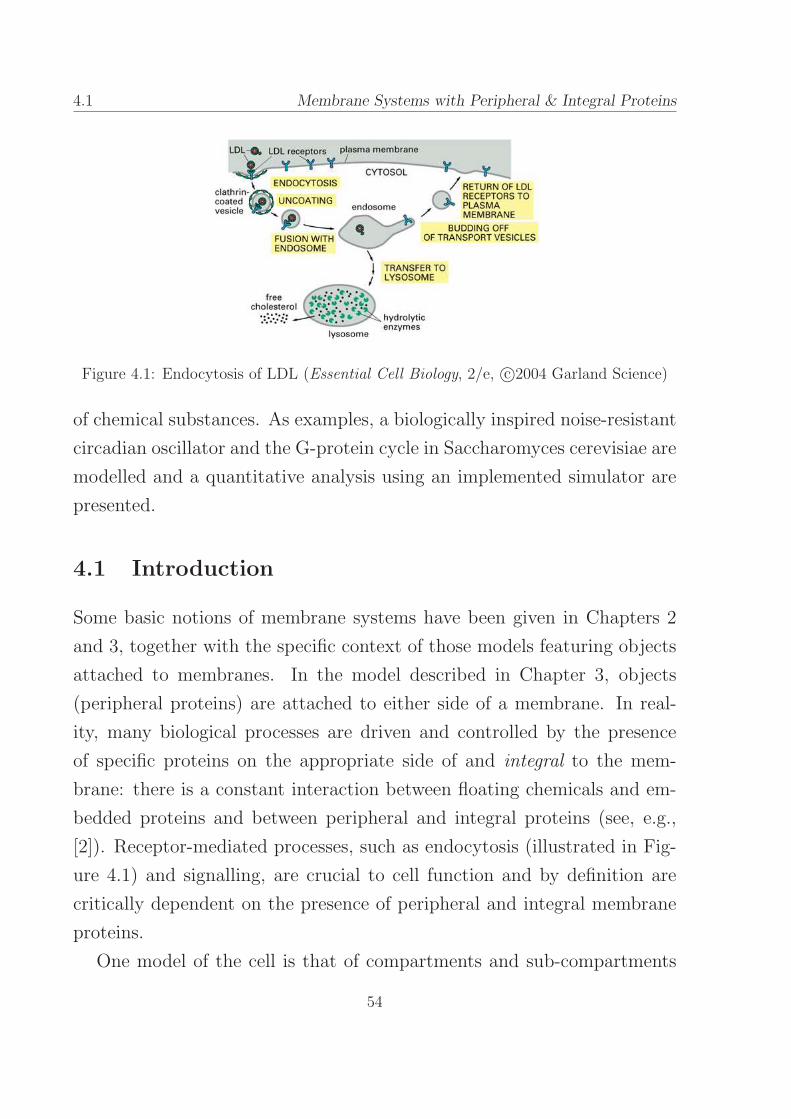
4.1 Membrane Systems with Peripheral & Integral Proteins
Figure 4.1: Endocytosis of LDL (Essential Cell Biology, 2/e, c©2004 Garland Science)
of chemical substances. As examples, a biologically inspired noise-resistant
circadian oscillator and the G-protein cycle in Saccharomyces cerevisiae are
modelled and a quantitative analysis using an implemented simulator are
presented.
4.1 Introduction
Some basic notions of membrane systems have been given in Chapters 2
and 3, together with the specific context of those models featuring objects
attached to membranes. In the model described in Chapter 3, objects
(peripheral proteins) are attached to either side of a membrane. In real-
ity, many biological processes are driven and controlled by the presence
of specific proteins on the appropriate side of and integral to the mem-
brane: there is a constant interaction between floating chemicals and em-
bedded proteins and between peripheral and integral proteins (see, e.g.,
[2]). Receptor-mediated processes, such as endocytosis (illustrated in Fig-
ure 4.1) and signalling, are crucial to cell function and by definition are
critically dependent on the presence of peripheral and integral membrane
proteins.
One model of the cell is that of compartments and sub-compartments
54
Membrane Systems with Peripheral & Integral Proteins 4.2
in constant communication, with molecules being passed from donor com-
partments to target compartments by interaction with membrane proteins.
Once transported to the correct compartment, the substances are then pro-
cessed by means of local biochemical reactions.
Motivated by these ideas the model presented in Chapter 3 is extended,
introducing a model having peripheral as well as integral proteins.
In each region of the system there are floating objects (the floating chem-
icals) and, in addition, objects can be associated to each side of a membrane
or integral to the membrane (the peripheral and integral membrane pro-
teins). Moreover, the system can perform the following operations: (i) the
floating objects can be processed/changed inside the regions of the system
(emulating biochemical rules) and (ii) the floating and attached objects
can be processed/changed when they interact (modelling the interactions
of the floating molecules with membrane proteins).
The proposed model can be used to represent cellular processes that
involve floating molecules, surface and integral membrane proteins, trans-
port of molecules across membranes and processing of molecules inside the
compartments. As examples, a biologically-inspired noise-resistant circa-
dian oscillator and the G-protein cycle in Saccharomyces cerevisiae are
modelled, where the possibility to use, in an explicit way, compartments,
membrane proteins and transport rules is very useful. A quantitative anal-
ysis of the models is also presented, performed using an extended version of
the simulator originally presented in [21] and described in Chapter 5. The
simulator employs a stochastic algorithm and uses intuitive syntax based
on chemical equations (described in Section 5.5).
In what follows it is assumed that the reader is already familiar with
the contents of Chapters 2 and 3.
55

4.2 Membrane Systems with Peripheral & Integral Proteins
4.2 Operations with Peripheral and Integral Proteins
This section presents operations on the MSPIP model and defines termi-
nology which will be used in the sequel. The membrane syntax and other
conventions are those described in Section 2.1.1.
Let V denote a finite alphabet of objects and Lab a finite set of labels.
In contrast to the model presented in Chapter 3, to each membrane
there are associated three multisets, u, v and x over V , denoted by [ ]u|v|x.
This is reported by saying that the membrane is marked by u, v and x; x
is called the external marking, u the internal marking and v the integral
marking of the membrane. In general, they are referred to as markings of
the membrane.
The internal, external and integral markings of a membrane model the
proteins attached to the internal surface, attached to the external surface
and integral to the membrane, respectively.
In a membrane structure, the region between membrane i and any en-
closed membranes is called region i. To each region is associated a multiset
of objects w called the free objects of the region. The free objects are writ-
ten between the brackets enclosing the regions, e.g., [ aa [ bb ]1 ]0.
The free objects of a membrane model the floating chemicals within the
regions of a cell.
int(i), ext(i) and itgl(i) denote the internal, external and integral mark-
ings of membrane i, respectively. free(i) denotes the free objects of region
i. For any membrane i, distinct from a root membrane, out(i) denotes the
label of the membrane enclosing membrane i.
For example, the string
[ ab [ cc ]2a| | [ abb ]1bba|ab|c ]0
represents a membrane structure, where to each membrane are associated
56

Membrane Systems with Peripheral & Integral Proteins 4.2
markings and to each region are associated free objects. Membrane 1 is
internally marked by bba (i.e., int(1) = bba), has integral marking ab (i.e.,
itgl(1) = ab) and is externally marked by c (i.e., ext(1) = c). To region
1 are associated the free objects abb (i.e., free(1) = abb). To region 0 are
associated the free objects ab. Finally, out(1) = out(2) = 0. Membrane 0
is the root membrane. The string can also be depicted diagrammatically,
as in Figure 4.2.
Figure 4.2: Graphical representation of membrane system [ ab [ cc ]2a| | [ abb ]1bba|ab|c ]0
When a marking is omitted it is intended that the membrane is marked
by the empty string λ, i.e., the empty multiset. For instance, in [ ab ]u|v|the external marking is missing, while in the case of [ ab ] |v|x the internal
marking is missing.
4.2.1 Operations
Rules are presented here that describe bidirectional interactions of floating
objects with the membrane markings and are called membrane rules. These
rules are motivated by the behaviour of cell membrane proteins (e.g., see
[2]) and therefore permit a level of abstraction based on the behaviour of
real molecules. The rules are denoted as attachin, attachout, de− attachin
and de− attachout, defined:
57
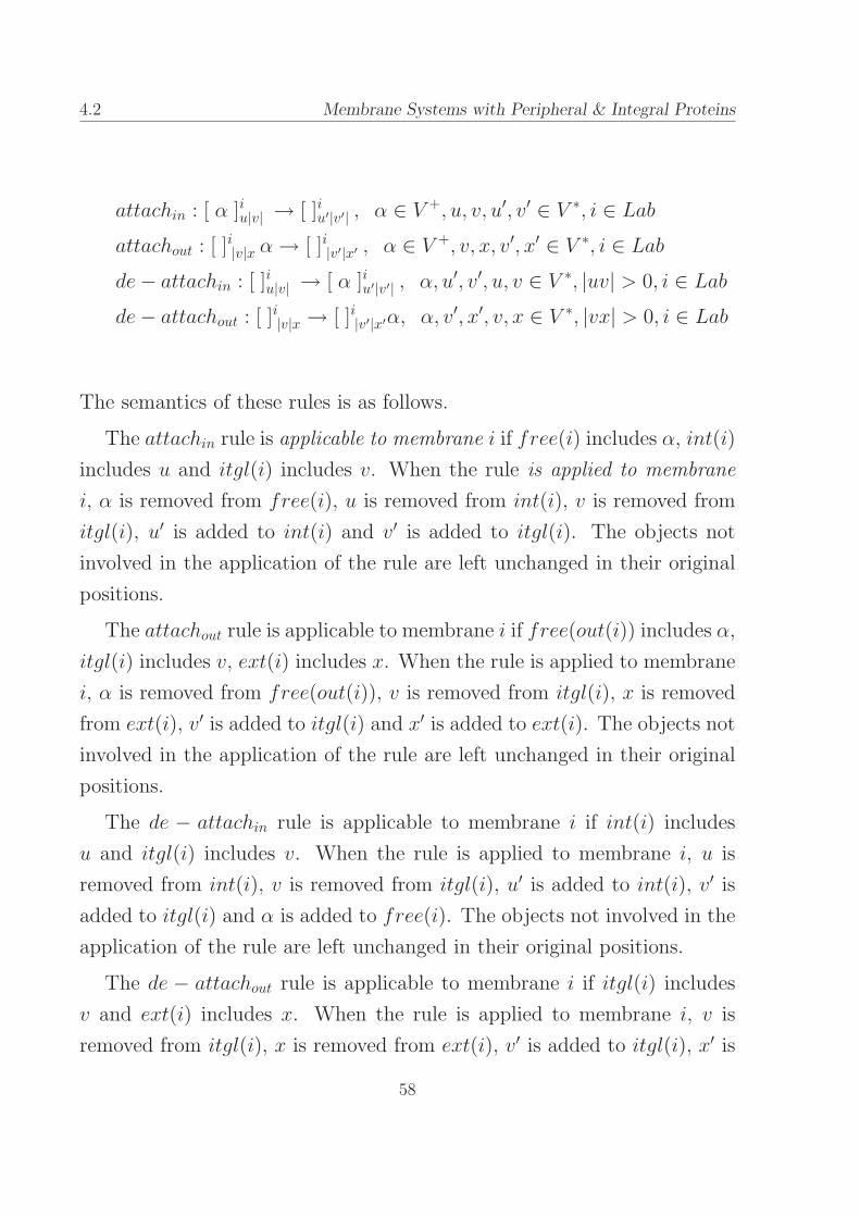
4.2 Membrane Systems with Peripheral & Integral Proteins
attachin : [ α ]iu|v| → [ ]iu′|v′| , α ∈ V +, u, v, u′, v′ ∈ V ∗, i ∈ Labattachout : [ ]i|v|x α→ [ ]i|v′|x′ , α ∈ V +, v, x, v′, x′ ∈ V ∗, i ∈ Labde− attachin : [ ]iu|v| → [ α ]iu′|v′| , α, u′, v′, u, v ∈ V ∗, |uv| > 0, i ∈ Labde− attachout : [ ]i|v|x → [ ]i|v′|x′α, α, v′, x′, v, x ∈ V ∗, |vx| > 0, i ∈ Lab
The semantics of these rules is as follows.
The attachin rule is applicable to membrane i if free(i) includes α, int(i)
includes u and itgl(i) includes v. When the rule is applied to membrane
i, α is removed from free(i), u is removed from int(i), v is removed from
itgl(i), u′ is added to int(i) and v′ is added to itgl(i). The objects not
involved in the application of the rule are left unchanged in their original
positions.
The attachout rule is applicable to membrane i if free(out(i)) includes α,
itgl(i) includes v, ext(i) includes x. When the rule is applied to membrane
i, α is removed from free(out(i)), v is removed from itgl(i), x is removed
from ext(i), v′ is added to itgl(i) and x′ is added to ext(i). The objects not
involved in the application of the rule are left unchanged in their original
positions.
The de − attachin rule is applicable to membrane i if int(i) includes
u and itgl(i) includes v. When the rule is applied to membrane i, u is
removed from int(i), v is removed from itgl(i), u′ is added to int(i), v′ is
added to itgl(i) and α is added to free(i). The objects not involved in the
application of the rule are left unchanged in their original positions.
The de − attachout rule is applicable to membrane i if itgl(i) includes
v and ext(i) includes x. When the rule is applied to membrane i, v is
removed from itgl(i), x is removed from ext(i), v′ is added to itgl(i), x′ is
58

Membrane Systems with Peripheral & Integral Proteins 4.2
attachin rule [ b ]ib|c| → [ ]idb|c| attachout rule [ ]i|c|a b→ [ ]i|c|ad
de− attachin rule [ ]ibb|c| → [ d ]ib|c| de− attachout rule [ ]i|c|a → [ ]i| |a d
Figure 4.3: Examples of attachin, attachout, de−attachin and de−attachout rules, showing
how free and attached objects may be rewritten. E.g., in the attachin rule one of the two
free instances of b is rewritten to d and added to the membrane’s internal marking.
added to ext(i) and α is added to free(out(i)). The objects not involved
in the application of the rule are left unchanged in their original positions.
RattV,Lab denotes the set of all possible attach and de− attach rules over
the alphabet V and set of labels Lab. Instances of attachin, attachout,
de− attachin and de− attachout rules are depicted in Figure 4.3.
Next are presented evolution rules that rewrite the free objects contained
in a region conditional on the markings of the enclosing membrane. These
rules can be considered to model the biochemical reactions that take place
within the cytoplasm of a cell. An evolution rule is defined thus:
evol : [ α→ β ]iu|v|
where u, v, β ∈ V ∗, α ∈ V +, and i ∈ Lab.The semantics of the rule is as follows. The rule is applicable to region i
if free(i) includes α, int(i) includes u and itgl(i) includes v. When the rule
is applied to region i, α is removed from free(i) and β is added to free(i).
59
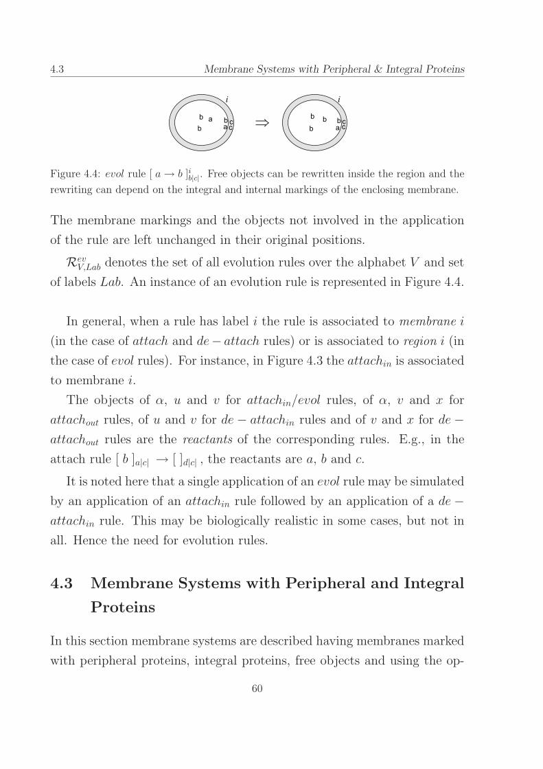
4.3 Membrane Systems with Peripheral & Integral Proteins
Figure 4.4: evol rule [ a→ b ]ib|c|. Free objects can be rewritten inside the region and the
rewriting can depend on the integral and internal markings of the enclosing membrane.
The membrane markings and the objects not involved in the application
of the rule are left unchanged in their original positions.
RevV,Lab denotes the set of all evolution rules over the alphabet V and set
of labels Lab. An instance of an evolution rule is represented in Figure 4.4.
In general, when a rule has label i the rule is associated to membrane i
(in the case of attach and de− attach rules) or is associated to region i (in
the case of evol rules). For instance, in Figure 4.3 the attachin is associated
to membrane i.
The objects of α, u and v for attachin/evol rules, of α, v and x for
attachout rules, of u and v for de − attachin rules and of v and x for de −attachout rules are the reactants of the corresponding rules. E.g., in the
attach rule [ b ]a|c| → [ ]d|c| , the reactants are a, b and c.
It is noted here that a single application of an evol rule may be simulated
by an application of an attachin rule followed by an application of a de−attachin rule. This may be biologically realistic in some cases, but not in
all. Hence the need for evolution rules.
4.3 Membrane Systems with Peripheral and Integral
Proteins
In this section membrane systems are described having membranes marked
with peripheral proteins, integral proteins, free objects and using the op-
60

Membrane Systems with Peripheral & Integral Proteins 4.3
erations presented in Section 4.2.
Definition 4.3.1 A membrane system with peripheral and integral pro-
teins and n membranes (in short, a Ppi system), is a construct
Π = (VΠ, µΠ, (u
0, v
0, x
0)
Π, . . . , (un−1, vn−1, xn−1)Π
, w0,Π, . . . , w
n−1,Π, RΠ,
tin,Π, t
fin,Π, rate
Π)
• VΠ is a finite, non-empty alphabet of objects.
• µΠ
is a membrane structure with n ≥ 1 membranes injectively labelled
by labels in LabΠ
= 0, 1, · · · , n − 1, where 0 is the label of the root
membrane.
• (u0, v0, x0)Π= (λ, λ, λ), (u
1, v
1, x
1)
Π, · · · , (un−1, vn−1, xn−1)Π
∈ V ∗×V ∗×V ∗ are called initial markings of the membranes.
• w0,Π, w
1,Π, · · · , w
n−1,Π∈ V ∗ are called initial free objects of the regions.
• RΠ ⊆ RattV,Lab
Π−0 ∪ Rev
V,LabΠ
is a finite set of evolution rules, attach
and de-attach rules.1
• tin,Π, t
fin,Π∈ R are called the initial time and the final time, respectively.
• rateΠ
: RΠ 7−→ R is the rate mapping. It associates to each rule a
rate.
Let Π be an arbitrary Ppi system. An instantaneous description I of Π
consists of the membrane structure µΠ
with markings associated to the
membranes and free objects associated to the regions. I(Π) denotes the
set of all instantaneous descriptions of Π. As a shorthand, membrane
(region) i of I denotes the membrane (region, respectively) i present in I.
1The root membrane may contain objects and evolution rules but not attach or de−attach rules, since
it has no enclosing region. It may therefore be viewed as an extended version of a membrane systems
environment (as defined in [72]), with objects and evol rules. Alternatively, it can be seen as a membrane
systems skin membrane, where the environment contains nothing and is not accessible.
61

4.3 Membrane Systems with Peripheral & Integral Proteins
Let I be an arbitrary instantaneous description from I(Π) and r an
arbitrary rule from RΠ. Suppose that r is associated to membrane i ∈ LabΠif r ∈ Ratt
V,LabΠ−0 (or to region i ∈ LabΠ if r ∈ RevV,LabΠ
).
Then, if r is applicable to membrane i (or to region i, accordingly) of
I, in short, r is applicable to I. r(I) ∈ I(Π) denotes the instantaneous
description of Π obtained when the rule r is applied to membrane i (or to
region i, accordingly) of I (in short, r is applied to I).
The initial instantaneous description of Π, Iin,Π ∈ I(Π), consists of the
membrane structure µΠ
with membrane i marked by (ui, vi, xi)Π for all
i ∈ LabΠ−0 and free objects wi,Π associated to region i for all i ∈ LabΠ.
A configuration of Π is a pair (I, t) where I ∈ I(Π) and t ∈ R; t is called
the time of the configuration. C(Π) denotes the set of all configurations of
Π. The initial configuration of Π is Cin,Π = (Iin,Π, tin,Π).
Suppose that RΠ = rule1, rule2, . . . , rulem and let S be an arbi-
trary sequence of configurations 〈C0, C1, · · · , Cj, Cj+1, · · · , Ch〉, where Cj =
(Ij, tj) ∈ C(Π) for 0 ≤ j ≤ h. Let aj =m∑
i=1
pij, 0 ≤ j ≤ h, where pi
j is the
product of rate(rulei) and the mass action combinatorial factor for rulei
and Ij (see Section 4.5).
The sequence S is an evolution of Π if
• for j = 0, Cj = Cin,Π
• for 0 ≤ j ≤ h− 1, aj > 0, Cj+1 = (rj(Ij), tj + dtj) with rj, dtj as in
[32]:
rj = rulek, k ∈ 1, · · · ,m and k satisfiesk−1∑
i=1
pij < ran
′
j ·aj ≤k
∑
i=1
pij
dtj = (−1/aj)ln(ran′′
j)
where ran′
j, ran′′
j are two random variables over the sample space (0, 1],
uniformly distributed.
62

Membrane Systems with Peripheral & Integral Proteins 4.4
• for j = h, aj = 0 or tj ≥ tfin,Π
.
In other words, an evolution of Π is a sequence of configurations, starting
from the initial configuration of Π, where, given the current configuration
Cj = (Ij, tj), the next one, Cj+1 = (Ij+1, tj+1), is obtained by applying the
rule rj to the current instantaneous description Ij and adding dtj to the
current time tj. The rule rj is applied as described in Section 4.2. Rule
rj and dtj are obtained using the Gillespie algorithm [32] over the current
instantaneous description Ij. The evolution halts when all rules have zero
probability of being applied (aj = 0) or when the current time is greater or
equal to the specified final time.
4.4 Modelling and Simulation of Cellular Processes
Having established a theoretical basis, it is now desirable to demonstrate
the quantitative behaviour of the presented model. To this end the sim-
ulator first presented in [21] was extended to produce evolutions of an
arbitrary Ppi system. In Sections 4.4.2 and 4.4.3 the model and the sim-
ulator are demonstrated using two examples from the literature. Chapter
5 contains a more detailed description of the simulator (Cyto-Sim) and
features many examples.
4.4.1 The Stochastic Algorithm
A discrete and stochastic simulation algorithm is employed, based on Gille-
spie’s, which can potentially represent the dynamical behaviour of small
quantities of reactants more accurately, in comparison, say, to a deter-
ministic approach based on ordinary differential equations [63]. Moreover,
Gillespie has shown that the algorithm is fully consistent with the chemical
master equation.
63

4.4 Membrane Systems with Peripheral & Integral Proteins
The Gillespie algorithm is specifically designed to model the interaction
of chemical species and imposes a restriction of a maximum of three react-
ing molecules. This is on the basis that the likelihood of more than three
molecules colliding is vanishingly small. Hence the simulator is similarly
restricted. Note that in the evolution of a Ppi system, the stochastic algo-
rithm does not distinguish between floating objects and objects attached or
integral to the membrane. That is, the algorithm is applied to the objects
irrespective of where they are in the compartment on the assumption that
the interaction between floating and attached molecules can be considered
the same as between floating molecules. The application of the Gillespie
algorithm to membranes is further described in Section 4.5.
4.4.2 Modelling a Noise-Resistant Circadian Oscillator
Many organisms use circadian clocks to synchronise their metabolisms to
a daily rhythm, however the precise mechanisms of implementation vary
from species to species. One common requirement is the need to maintain
a measure of stability of timing in the face of perturbations of the system:
the clock must continue to tick and keep good time. A general model which
captures the essence of such stability, based on common elements of sev-
eral real biological oscillators, is presented in [84]. This is chosen as an
interesting, non-trivial example to model and simulate with a Ppi system
using evolution rules alone. Moreover, this example has been chosen be-
cause it has also been modelled in other formalisms, such as in stochastic
Π calculus (see, e.g., [86], [76]).
The model is described diagrammatically in Figure 4.5. The system
consists of two different genes (gA and gR) which produce two different
proteins (pA and pR, respectively) via two different mRNA species (mA and
mR, respectively). Protein pA up-regulates the transcription of its own gene
and also the transcription of the gene that produces pR. The proteins are
64

Membrane Systems with Peripheral & Integral Proteins 4.4
removed from the system by simple degradation to nothing (dashed lines)
and by the formation of a complex AR. In this latter way the production
of pR reduces the concentration of pA and has the consequence of down-
regulating pR’s own production. Thus, in turn, pA is able to increase,
increasing the production of pR and causing the cycle to repeat. Key
elements of the stable dynamics are the rapid production of pA, by virtue
of positive feedback, and the relative rate of growth of the complexation
reaction.
A description of the Ppi system used to model the circadian oscillator
is given in Figure 4.6, together with the corresponding simulator script for
comparison. The alphabet, Vclock, is specified to contain all the reacting
species. This corresponds to the object statement of the simulator script.
The sixteen chemical reactions of Figure 4.5 are simply transcribed into
corresponding rules mapped to reaction rates. In the simulator script they
are grouped under one identifier, clock. The membrane structure, µclock,
comprises just the root membrane. The root region initially contains one
copy each of the two genes as free objects. These facts are reflected in
the system statement of the simulator script, which also associates to the
contents the set of rules clock.
The results of running the script are shown in Figure 4.5: the two pro-
teins exhibit anti-phase periodicity of approximately 24 hours, as expected.
The simulator has the capability to add or subtract reactants from the
simulation in runtime. This facility is used to discover the effect of switch-
ing off gR in the circadian oscillator by making the following addition to
the system statement:
-1 gR @50000, -1 g R @50000
These instructions request a subtraction from the system at time step 50000
of one gR and one g R. Note that to switch off the gene it is necessary
to remove both versions (i.e., with and without pA bound), since it is
65

4.4 Membrane Systems with Peripheral & Integral Proteins
Figure 4.5: Reaction scheme and simulation results of noise-resistant circadian oscillator
of [84]
not possible to know in what state it will exist at a particular time step.
Negative quantities are not allowed in the simulator, so only the existent
specie will be deleted. In general, the number subtracted is the minimum of
the existent quantity and the requested amount. The same syntax, without
the negative sign, is used to add reactants.
The effect of switching off gR, shown in Figure 4.7, is to reduce the
amount of pR to near zero and to thus allow pA to reach a maximum
governed by its relative rates of production and decay. Note that a small
amount of pR continues to exist long after its gene has been switched off.
This is the result of a so-called hidden pathway from the AR complex,
which decays at a much slower rate than pR (second graph of Figure 4.7).
Although this model is a generalisation of biological circadian oscillators
and may not represent the behaviour of a specific example, the existence
of an unexpected pathway exemplifies an important problem encountered
when attempting to predict the behaviour of biological systems.
66

Membrane Systems with Peripheral & Integral Proteins 4.4
4.4.3 Modelling Saccharomyces Cerevisiae Mating Response
To demonstrate the ability of Ppi systems to abstract the notions compart-
ments and membranes found in biological systems, the G-protein mating
response in yeast Saccharomyces cerevisiae has been modelled and simu-
lated, based on experimental rates provided by [92]. The G-protein trans-
duction pathway involves membrane proteins and the transport of sub-
stances between regions and is a mechanism by which organisms detect
and respond to environmental signals. It is extensively studied and many
pharmaceutical agents are aimed at components of the G-protein cycle in
humans. The diagram in Figure 4.8 shows the relationships between the
various reactants and regions modelled and simulated.
A description of the biological process is that the yeast cell receives a
signal ligand (pL) which binds to a receptor pR, integral to the cell mem-
brane. The receptor-ligand dimer then catalyses (dotted line in the dia-
gram of Figure 4.8) the reaction that converts the inactive G-protein Gabg
to the active GA. A competing sequence of reactions, which dominate in
the absence of RL, converts GA to Gabg via Gd in combination with Gbg.
The bound and unbound receptor (RL and pR, respectively) are degraded
by transport into a vacuole via the cytoplasm. Figure 4.9 contains the Ppi
system model and corresponding simulator script. Note that while addi-
tional quantities of the receptor pR are created in runtime, no species is
deleted from the system; the dynamics are created by transport alone.
Figure 4.8 shows the results of a single stochastic simulation run plotted
with experimental results from [84] equivalent to simulated GA. There is an
apparent correspondence between the simulated and experimental data,
in line with the deterministic simulation presented in the original paper.
The stochastic noise evident in Figure 4.8 may explain why some measured
points do not lie exactly on the deterministic curve. Testing this hypothesis
67

4.5 Membrane Systems with Peripheral & Integral Proteins
would require multiple simulation runs in order to estimate a distribution
at the times of each measured point, however such analysis is beyond the
scope of this chapter.
4.5 Perspectives
A model of membrane systems (called a Ppi system) has been presented
with objects integral to the membrane and objects attached to either side
of the membrane. Operations have also been presented that can rewrite
floating objects conditional on the existence of integral and attached ob-
jects and operations that facilitate the interaction of floating objects with
integral and attached objects. With these it is possible to model in detail
many real biochemical processes occurring in the cytoplasm and in the cell
membrane.
Evolutions of a Ppi system are obtained using an algorithm based on
Gillespie [32] and in the second part of the chapter a simulator has been
presented which can produce evolutions of an arbitrary Ppi system, using
syntax based on chemical equations. To demonstrate the utility of Ppi
systems and of the simulator, a circadian oscillator and the G-protein cycle
mating response of Saccharomyces cerevisiae have been modelled. The
latter makes extensive use of membrane operations.
Several different research directions are now proposed. The primary direc-
tion is the application of Ppi systems and of the simulator to real biological
systems, with the aim of prediction by in-silico experimentation. Such ap-
plication is likely to lead to the need for new bio-inspired features and
these constitute another direction of research. The features will be im-
plemented in the model and simulator as necessary, however it is already
envisaged that operations of fission and fusion will be required to permit
the modification of a membrane structure in runtime.
68
Membrane Systems with Peripheral & Integral Proteins 4.5
A further direction of research is the investigation of the theoretical
properties of the model. Reachability of configurations and of markings
have already been proved to be decidable for the more restricted model
presented in Chapter 3 and these proofs should be extended accordingly
for the model presented here. Other work in this area might include the
modification of the way a Ppi system evolves, for example, to allow other
semantics (such as that of maximal parallel described in Chapter 3) or
to use algorithms that more accurately model the behaviour of biological
membranes. In this way it will be possible to explore the limits of the
model and perhaps discover a more useful level of abstraction.
Appendix to Chapter 4
The Gillespie Algorithm Applied To Membranes
The Gillespie algorithm is an exact stochastic simulation of a ‘spatially ho-
mogeneous mixture of molecular species which inter-react through a speci-
fied set of coupled chemical reaction channels’ [32]. It is unclear whether a
biological cell contains a spatially homogeneous mixture of molecular species
and less clear still whether integral and peripheral proteins can be described
in this way, however for the purposes of the Ppi system model, this is the
abstraction that has been chosen. Hence the objects attached to the mem-
brane are treated as being homogeneously mixed with the floating objects,
however objects of the same type (i.e. having the same name) but existing
in different regions are considered to be of different types in the stochastic
algorithm.
The mass action combinatorial factors of the Gillespie algorithm, de-
fined by equations (14a. . . g) in [32], are calculated over the set of chemical
reactions given in equations (2a. . . g) of [32], using standard stoichiometric
69
4.5 Membrane Systems with Peripheral & Integral Proteins
syntax of the general form
S1 + S2 + S3 → P1 + P2 + . . .+ Pn
S1, S2 and S3 are the reactants and P1, . . . , Pn are the products of the
reaction. Since the order of the reactants and products is unimportant
they may be represented as multisets S1S2S3 and P1P2 · · ·Pn, respectively,
over the set of objects V . Hence a chemical reaction may be expressed
using the notation
S1S2S3 → P1P2 · · ·Pn
In the definition of the evolution of a Ppi system, the mass action combina-
torial factor is calculated using equations (14a. . . g)[32] after transforming
the membrane and evolution rules into chemical reactions and the objects
of the current instantaneous description, using the following procedure.
Let Vi = ai|a ∈ V , Vi,int = ai,int|a ∈ V , Vi,itgl = ai,itgl|a ∈ V and Vi,out = ai,out|a ∈ V . Then define morphisms freei : V → Vi,
inti : V → Vi,int, itgli : V → Vi,itgl and outi : V → Vi,out such that
freei(a) = ai, inti(a) = ai,int, itgl
i(a) = ai,itgl and outi(a) = ai,out for
a ∈ V . Hence map an evolution rule of the type
[ α→ β ]iu|v|
with u, v, α, β ∈ V ∗ and i ∈ Lab, to the chemical reaction
freei(α) · inti(u) · itgli(v)→ freei(β) · inti(u) · itgli(v)
Map membrane rules, generally described by
[ α ]iu|v|x β → [ α′ ]iu′|v′|x′ β′
with u, v, x, α, β, u′, v′, x′, α′, β′ ∈ V ∗ and i ∈ Lab, to the chemical equation
freei(α) · inti(u) · itgli(v) · outi(x) · freej(β)→
70

Membrane Systems with Peripheral & Integral Proteins 4.5
freei(α′) · inti(u′) · itgli(v′) · outi(x′) · freej(β′)
where j ∈ Lab is the marking of the membrane surrounding the region
enclosing membrane i.
The objects of the current instantaneous description are similarly trans-
formed, using the morphisms defined above, in order to correspond with
the transformed membrane and evolution rules.
71

4.5 Membrane Systems with Peripheral & Integral Proteins
Ppi system clock Simulator script
Vclock = gA, g A, gR, g R,mA,mR, pA, pR,RA object gA,g A,gR,g R,mA,mR,pA,pR,RA
rateclock = rule clock
[ gA→ gA mA ]0| | 7→ 50 gA 50-> gA + mA
[ pA gA→ g A ]0| | 7→ 1 pA+gA 1-> g A
[ g A→ g A mA ]0| | 7→ 500 g A 500-> g A + mA
[ gR→ gR mR ]0| | 7→ 0.01 gR 0.01-> gR + mR
[ g R→ g R mR ]0| | 7→ 50 g R 50-> g R + mR
[ mA→ pA ]0| | 7→ 50 mA 50-> pA
[ mR→ pR ]0| | 7→ 5 mR 5-> pR
[ pA pR→ AR ]0| | 7→ 2 pA+pR 2-> AR
[ AR→ pR ]0| | 7→ 1 AR 1-> pR
[ pA→ λ ]0| | 7→ 1 pA 1-> 0A
[ pR→ λ ]0| | 7→ 1 pR 0.2-> 0R
[ mA→ λ ]0| | 7→ 10 mA 10-> 0mA
[ mR→ λ ]0| | 7→ 0.5 mR 0.5-> 0mR
[ g R→ pA gR ]0| | 7→ 100 g R 100-> pA+gR
[ pA gR→ g R ]0| | 7→ 1 pA+gR 1-> g R
[ g A→ pA gA ]0| | 7→ 50 g A 50-> pA+gA
w0,clock = gA gR system 1 gA, 1 gR, clock
µclock = [ ]0
tin,clock = 0 evolve 0-150000
tfin,clock = 155 hours
plot pA, pR
Figure 4.6: Ppi system model of circadian oscillator of [84] with corresponding simulator
script. Note the similarities between the definitions of Vclock and object and between the
definitions of the elements of rateclock and of rule clock.
72

Membrane Systems with Peripheral & Integral Proteins 4.5
Figure 4.7: Simulated effect of switching off gA in circadian oscillator of [84]
Diagrammatic representation of model. Simulation results (continuous curves) and
experimental data (points with error bars, [92])
corresponding to simulated GA. Note: Gd decays
rapidly and is not visible at this scale.
Figure 4.8: Model and simulation results of Saccharomyces cerevisiae mating response.
73

4.5 Membrane Systems with Peripheral & Integral Proteins
Ppi system gprot Simulator script
Vgprot = pL, pr, pR,RL,Gd,Gbg,Gabg,GA object pL,pr,pR,RL,Gd,Gbg,Gabg,GA
rategprot = rule g cycle
[ ]1|pr| → [ ]1|pR pr| 7→ 4.0 |pr| 4-> |pR,pr|
[ ]1|pR| pL→ [ ]1|RL| 7→ 3.32e−18 |pR| + pL 3.32e-18-> |RL|
[ ]1|RL| → [ ]1|pR| pL 7→ 0.011 |RL| 0.011-> |pR| + pL
[ ]1|RL| → [ RL ]1| | 7→ 4.1e−3 |RL| 4.1e-3-> RL + ||
[ ]1|pR| → [ pR ]1| | 7→ 4.1e−4 |pR| 4.1e-4-> pR + ||
[ Gabg → GA Gbg ]1|RL| 7→ 1.0e−5 Gabg + |RL| 1.0e-5-> GA, Gbg + |RL|
[ Gd Gbg → Gabg ]1| | 7→ 1.0 Gd + Gbg 1-> Gabg
[ GA→ Gd ]1| | 7→ 0.11 GA 0.11-> Gd
rule vac rule
[ ]2| | pR→ [ pR ]2| | 7→ 4.1e−4 || + pR 4.1e-4-> pR + ||
[ ]2| | RL→ [ RL ]2| | 7→ 4.1e−3 || + RL 4.1e-3-> RL + ||
w2,gprot = λ compartment vacuole [vac rule]
(u2, v2, x2)gprot = (λ, λ, λ)
w1,gprot = Gd3000 Gbg3000 Gabg7000 compartment cell[vacuole,3000 Gd,...
(u1, v1, x1)gprot = (λ, pR10000pr, λ) 3000 Gbg,7000 Gabg,g cycle:|10000 pR,pr|]
w0,gprot = pL6.022e17 system cell, 6.022e17 pL
µgprot = [ [ [ ]2 ]1 ]0
tin,gprot = 0 evolve 0-600000
tfin,gprot = 600 seconds
plot cell[Gd,Gbg,Gabg,GA:|pR,RL|]
Figure 4.9: Ppi system model of G-protein cycle and corresponding simulator script.
74

Chapter 5
Cyto-Sim
Some of the work presented in this chapter was originally published in
S. Sedwards and T. Mazza (2008) Cyto-Sim: A formal language model and stochastic simulator
of membrane-enclosed biochemical processes, Bioinformatics, 23:20, 2800–2802.
Compartments and membranes are the basis of cell topology and more
than 30% of the human genome codes for membrane proteins. It is possi-
ble to represent compartments and membrane proteins in a nominal way
with many mathematical formalisms used in systems biology, however few
explicitly model the topology of the membranes themselves.
Discrete stochastic simulation of molecular kinetics potentially offers the
most accurate representation of cell dynamics. Since the details of every
molecular interaction in a pathway are often not known, the relationship
between chemical species in not necessarily best described by simple mass
action chemistry. Moreover, modelling every individual molecular interac-
tion in the cell is probably unnecessary and currently impractical.
Simulation is a form of computer aided analysis, relying on human in-
terpretation to derive meaning. To improve efficiency and gain meaning in
an automatic way, it is necessary to have a formalism based on a model
which has decidable properties.
Cyto-Sim is a stochastic simulator of hierarchies of membrane-enclosed
75

5.1 Cyto-Sim
biochemical processes, where the membranes comprise an inner, outer and
integral layer. The full underlying model is presented in Chapter 4, while
the version of the model presented in Chapter 3 has been shown to have
decidable properties in Chapter 3, allowing formal analysis in addition to
simulation. The simulator provides arbitrary levels of abstraction based on
chemical kinetics and ordinary differential equations; these latter providing
a further dimension of analysability.
The paradigm is flexible and extensible, permitting adaptation to other
types of simulation and analysis and integration within standard platforms.
In addition to its compact native syntax, based on stoichiometric equations
and reaction kinetics, Cyto-Sim currently supports models described as
Petri nets, can import all versions of SBML and can export SBML and
MATLAB R© m-files.
5.1 Introduction
The function of membranes in cells is fundamental to their activity, sepa-
rating them from other cells to permit differentiation of function and sepa-
rating organelles within cells for similar purposes. Membrane proteins reg-
ulate the communication between the membrane-enclosed compartments
and play a statistically important role in cell activity: more than 30% of
the human genome codes for membrane proteins. Since membrane proteins
control the entry of susbtances to cells, it is no surprise that in 2000 almost
50% of the drugs prescribed in the USA targetted one class of membrane
proteins alone (GPCRs).
In computational terms, compartments correspond to scope, that is, re-
gions where calculations can be performed in a local context. In computer
programs, scope is the basis of functions, which are a means to perform
the same calculation on different data without creating new code - com-
76
Cyto-Sim 5.2
putational differentiation. Biology has a finite repertoire of molecules to
perform its calculations and uses compartments to increase computational
power in the same way, i.e., by having a multiplicity of membrane-enclosed
cells.
The aim is to create predictive or otherwise useful models of biologi-
cal processes, with the current focus on inter- and intracellular pathways.
Recognising the important roles of membrane proteins and biological scope,
a model is required that allows the simultaneous representation of different
(types of) cells which communicate via ligands and receptors. In addition
to the obvious biological analogues, membranes can also be used to repre-
sent notional compartments in order to characterise, for example, diffusion
or localised behaviour. Further, compartments can be used like assay plate
wells, enabling several experiments to be run simultaneously and efficiently.
These ideas and other have previously been considered, for example, in [22]
and [25].
5.2 Approach
The formal basis for the simulator model has been presented in Chapter 4.
The default level of abstraction in the implementation is thus chemistry:
objects interact governed by stoichiometric rules at a rate defined by mass
action kinetics. A variable level of abstraction is facilitated by the use of
arbitrary kinetic laws: objects are consumed and produced at rates defined
by arbitrary functions of reactants, thus modelling behaviour rather than
mechanism. This allows complex systems to be reduced to single equations
that nevertheless remain in the formal language and Markov framework
for analysis. Such reduction may be a necessity if the structure of the
system is unknown, or may be used to gain efficiency when the structure
is unimportant.
77

5.3 Cyto-Sim
The native simulator syntax language aims to be intuitive and unclut-
tered (see the description in Section 5.5). Objects, rules and compartments
are defined, then (a subset of) these are composed to create the final sys-
tem to simulate. In this way it is not necessary to explicitly define rules
and objects for each compartment, as is necessary, for example, in SBML.
Petri nets are an intuitive graphical representation of logical flows, which
have been successfully applied to biology (e.g., [66]). Hence, in addition
to the native rule syntax, the simulator supports rule definitions in the
form of Petri net incidence matrices. There is strong correspondence be-
tween stochastic Petri nets and stochastic chemical rules so, by default,
the transitions adopt mass action kinetics, i.e., the rate of the transition
is proportional to a constant multiplied by the numbers of tokens in the
incoming places. Other Petri net dynamics are also possible by explicitly
defining appropriate kinetic laws.
5.3 Methods
The software is written in J#, a Java-like language which is part of the
.NET framework. This choice allows easy porting to both Java and C#
and hence maximises cross-platform compatibility. There are currently two
versions available on the internet [87]; an applet and a standalone version,
both implemented in Java and having a graphical user interface (GUI).
Other versions can be made available upon request.
The core simulation engine is an efficient implementation of a Markov
chain Monte Carlo algorithm, based on that of Gillespie [33]. Performance
is optimised for mass action chemical kinetics, however the simulator also
supports chemical reactions with arbitrary kinetic laws based on functions
of the reactants. This latter restriction guarantees the Markov property
but permits the use of the many alternative kinetic laws used in systems
78

Cyto-Sim 5.4
biology. The addition of arbitrary kinetic laws is achieved in an efficient
way, based on compiler technology and a virtual machine, and does not
adversely affect the performance of the default kinetics.
5.4 Discussion
Much of the modelling in systems biology is done in the framework of
deterministic differential equations, which are usually solved by numerical
methods. Such solutions might more accurately be described as deter-
ministic simulations. Recognising that molecular interactions are discrete
stochastic events and that this stochasticity has a significant effect on the
behaviour of models which have neutral or unstable manifolds [33], dis-
crete stochastic simulations are now often used to give a more accurate
representation of such behaviour. The principal qualitative difference be-
tween the two approaches is that, for a given set of simulation parameters,
a deterministic simulation will have a unique, average, solution, whereas
a discrete stochastic simulation is a single trajectory through the solution
space. By using Monte Carlo techniques, the stochastic trajectory is guar-
anteed to be statistically consistent with the master equation describing
the system, however this does not guarantee that a particular behaviour
will be observed in any given simulation. Hence, a deterministic simulation
gives a single average characterisation of the system but may not charac-
terise all the behaviour, whereas a discrete stochastic simulation is only
guaranteed to display all the behaviour in the limit of simulations. The
choice between these two techniques is therefore dependent on the quality
and robustness of the behaviour and the types of manifold present. Given
that some robust behaviour may not be observed in a deterministic simula-
tion, e.g., behaviour that relies on a stochastic divergence at a bifurcation
point, performing many stochastic simulations is usually preferable. The
79

5.5 Cyto-Sim
efficiency of the Cyto-Sim algorithm, which can outperform the determinis-
tic simulation of some models (particularly those with many reactions and
low molecular concentrations, see Table 5.1) makes such statistical analysis
feasible. In Cyto-Sim, models can also be exported as sets of differential
equations in the form of a MATLABR© m-file. So, having performed initial
stochastic simulations, it is thus possible to perform algebraic or numerical
analysis or, at least, deterministic simulation, to gain further insight about
the system.
Simulator Yeast G prot. cycle N-R oscillator
Cyto-Sim 1.1s 0.41s
CellDesigner1 1.5s 2.2s
MATLAB R©2 (deterministic) 617s 6.3s
Dizzy3 1013s (Dizzy estd.) 19.3s
(Windows XP, JRE 1.6, Centrino M, 1.6GHz, 2MB L2 cache, 512 MB RAM)
1www.celldesigner.org 2www.mathworks.com 3www.systemsbiology.org
Table 5.1: Timings of Cyto-Sim and other popular simulators with models of yeast G
protein coupled cycle [92] and a noise-resistant oscillator [84]. Simulated times were 600
seconds and 250 hours, respectively.
5.5 The Cyto-Sim language
The Cyto-Sim language syntax aims to be an intuitive interpretation of
the Ppi system model presented in Chapter 4 and to provide sophisticated
controls and ease of use to modellers. A simulator script conforms to the
following grammar:
80

Cyto-Sim 5.5
Simulator Script = Constant Declaration Object Declaration Object Declaration ( Rule Definition Rule Definition | Petri Net Definition )
Compartment Definition System Statement
Evolve Statement
Plot Statement
An example of a simple simulator script is shown below, together with
its Ppi system counterpart.
Simulator script Ppi system lotka
// Lotka reactions
object X,Y1,Y2,Z Vlotka = X, Y 1, Y 2, Zratelotka =
rule r1 X + Y1 0.0002-> 2Y1 + X [ XY 1→ Y 1Y 1X ]0| | 7→ 0.0002
rule r2 Y1 + Y2 0.01-> 2Y2 [ Y 1Y 2→ Y 2Y 2 ]0| | 7→ 0.01
rule r3 Y2 10-> Z [ Y 2→ Z ]0| | 7→ 10 system 100000 X,1000 Y1,1000 Y2,r1,r2,r3 w0,lotka = X100000Y 11000Y 21000
µlotka = [ ]0
evolve 0-1000000 tin,lotka = 0
plot Y1,Y2
The syntax of the various sections of a simulator script are described
below.
5.5.1 Comments
Comments begin with a double forward slash (//) and include all subse-
quent text on a single line. They may appear anywhere in the script.
81
5.5 Cyto-Sim
5.5.2 Constant Declaration
A constant declaration uses the keyword constant and contains a comma
separated list of unique identifiers and assignments to define values which
do not change. E.g.:
constant k1=0.0002,k2=0.01,k3=10
The constant declaration serves to perform both the declaration of an iden-
tifier as a constant and the assignment of its value. The right hand side of
the assignment may be a mathematical expression containing literal values
and previously defined constants. E.g.:
constant alpha=6.023e-17,x=0.1*alpha,y=0.02*alpha
Any number of consecutive constant declarations are permitted.
5.5.3 Object Declaration
The reacting objects are defined in one or more statements beginning with
the keyword object followed by a comma separated list of unique reactant
names. E.g.:
object X,Y1,Y2,Z
The names are case-sensitive and must start with a letter but may include
digits and the underscore character ( ). This corresponds to defining the
alphabet V of the Ppi system.
5.5.4 Rule Definition
The reaction rules are defined using rule definitions comprising the keyword
rule followed by a unique name and the rewriting rule itself. E.g.:
rule r1 X + Y1 0.0002-> 2Y1 + X
These correspond to the attach / de-attach and evolution rules of the Ppi
system model. Here r1 is the name of the rule and X and Y1 are the
82

Cyto-Sim 5.5
names of objects. Note, however, that simulator rules are user-defined
types which may be instantiated in more than one region. The value pre-
ceding the implication symbol (->) is the average mass action reaction rate
and corresponds to an element of the range of the mapping rate given in
Definition 4.3.1. In the simulator it is also possible to define a reaction
rate as the product of a constant and the rate of a previously defined rule,
using the name of the previous rule in the following way:
rule r2 Y1 + Y2 50 r1-> 2Y2
This has the meaning that rule r2 has a rate 50 times that of r1. In
addition, in the simulator it is possible to define a group of rules using a
single identifier and braces. E.g.,
rule lotka
X + Y1 0.0002-> 2Y1 + X
Y1 + Y2 0.01-> 2Y2
Y2 10-> Z
To include membrane operations the simulator rule syntax is extended with
| symbols to denote the membrane, in a deliberately similar way to that
described in Section 2.1.1. In general, the membrane is represented by ||;
objects listed on the left hand side of the || represent the internal markings,
objects listed on the right hand side represent the external markings and
objects listed between the vertical bars are the integral markings of the
membrane. E.g.:
rule r4 X + |Y2| 0.1-> |X,Y2|
means that if one X exists within the compartment and one Y2 exists inte-
gral to the membrane, then the X will be added to the integral marking of
the membrane. The Ppi system equivalent is the following attachin rule:
[ X ] |Y 2| → [ ] |XY 2|
83

5.5 Cyto-Sim
To represent an attachout rule in the simulator the following syntax is
used:
rule r4 |Y2| + X 0.1-> |X,Y2|
Here the X appears to the right of the || symbol following a +, meaning
that it must exist in the region surrounding the membrane for the rule
to be applied. Hence the + used in simulator membrane rules is non-
commutative.
Arbitrary kinetics
Rules can be specified using kinetics other than mass action by writing a
suitable parenthesis-enclosed function in place of the rate. E.g.:
rule enzyme E + S (Vmax*S/(S+Km))-> E + P
is an archetypal Michaelis-Menten reaction, where it is assumed that Vmax
and Km are previously defined constants. The S used within the function
refers to the object of the same name; during the simulation this variable
takes the value of the current number of S objects in the local context of
the rule. While one E and one S must exist for the rule to be applicable,
the rate of the rule is given entirely by the function contained within the
parenthesis. In general, this function need not necessarily refer to the
objects on the left hand side of the rule. Cyto-Sim implements the following
standard mathematical operations for use in arbitrary kinetic functions:
+, -, *, /, ^ (exponentiation) and (. . . ) (parentheses). Note that if an
arbitrary kinetic function produces a negative rate, a rate of zero is used.
5.5.5 Petri Net Definition
An entire set of rules may be specified as a Petri net using the keyword
petri and defining its incidence matrix. E.g.:
petri lotka_volterra
84

Cyto-Sim 5.5
X ,Y1,Y2,Z
t1 0 ,1 ,0 ,0 :(0.0002*X*Y1)
t2 0 ,-1,1 ,0 :(0.01*Y1*Y2)
t3 0 ,0 ,-1,1 :10
The keyword petri is thus used to define a block of rules having a single
name (the name of the network). Within the block delimited by braces,
the first line is a list of objects which define the data columns of the sub-
sequent matrix. The first column of the matrix contains the names of the
transitions which correspond to the rows. The rows are filled by comma
separated values defining whether tokens are consumed (negative) or pro-
duced (positive) by the transition. Each row is terminated by a colon
followed by a mass action rate, which may be replaced by a parenthesis-
enclosed arbitrary kinetic function, as described in Section 5.5.4. In the
case of enzymatic transitions, where an object is necessary but not con-
sumed, the incidence matrix is ambiguous: the zero entry could also mean
that the species is not involved. Under these circumstances the default
mass action kinetics will be incorrectly calculated and it is necessary to
write an explicit arbitrary kinetic function, as shown for transitions t1
and t2 in the above example.
5.5.6 Compartment Definition
Compartments may be defined using the keyword compartment followed
by a unique name and a list of contents and rules, all enclosed by square
brackets. For example,
compartment c1 [100 X, 100 Y1, r1, r2]
instantiates a compartment having the label c1 containing 100 X, 100 Y1
and rules r1 and r2. In a Ppi system such a compartment would have a
Ppi system (partial) initial instantaneous description
85
5.5 Cyto-Sim
[ X100Y 1100 ]1
Note that a Ppi system requires a numerical membrane label and that any
rules associated to the region or membrane must be defined separately.
Compartments may contain other pre-defined compartments, so the fol-
lowing simulator statement
compartment c2 [100 Y2, c1]
corresponds to the Ppi system (partial) initial instantaneous description
[ Y 2100[ X100Y 1100 ]1 ]2
Membrane markings in the simulator are added to compartment definitions
using the symbol ||, to the right of and separated from the floating contents
by a colon. E.g.,
compartment c3 [100 X, c2 : 10 Y2||10 Y1]
has the meaning that the compartment c3 contains compartment c2, 100
X, and the membrane surrounding c3 has 10 Y2 attached to its inner surface
and 10 Y1 attached to its outer surface. This corresponds to the Ppi system
(partial) initial instantaneous description
[ X100[ Y 2100[ X100Y 1100 ]1 ]2 ]3Y 210| |Y 110
5.5.7 System Statement
The system is instantiated using the keyword system followed by a comma-
separated list of constituents. E.g.:
system 100000 X,1000 Y1,1000 Y2,r1,r2,r3
This statement corresponds to the definition of u0 . . . un, v0 . . . vn, w0. . . wn,
x0 . . . xn and µ of the Ppi system.
The system statement may be extended to multiple lines by enclosing
the list of constituents between braces. E.g.:
86
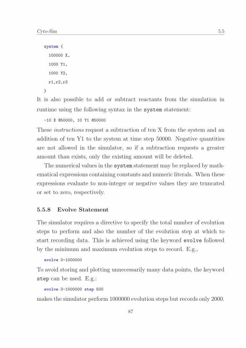
Cyto-Sim 5.5
system
100000 X,
1000 Y1,
1000 Y2,
r1,r2,r3
It is also possible to add or subtract reactants from the simulation in
runtime using the following syntax in the system statement:
-10 X @50000, 10 Y1 @50000
These instructions request a subtraction of ten X from the system and an
addition of ten Y1 to the system at time step 50000. Negative quantities
are not allowed in the simulator, so if a subtraction requests a greater
amount than exists, only the existing amount will be deleted.
The numerical values in the system statement may be replaced by math-
ematical expressions containing constants and numeric literals. When these
expressions evaluate to non-integer or negative values they are truncated
or set to zero, respectively.
5.5.8 Evolve Statement
The simulator requires a directive to specify the total number of evolution
steps to perform and also the number of the evolution step at which to
start recording data. This is achieved using the keyword evolve followed
by the minimum and maximum evolution steps to record. E.g.,
evolve 0-1000000
To avoid storing and plotting unnecessarily many data points, the keyword
step can be used. E.g.:
evolve 0-1000000 step 500
makes the simulator perform 1000000 evolution steps but records only 2000.
87

5.6 Cyto-Sim
All the numerical values in the evolve statement can be replaced by
mathematical expressions containing constants and numeric literals. When
these expressions evaluate to non-integer or negative values they are trun-
cated or set to zero, respectively.
Note that the minimum evolution step does not correspond to tin of
the Ppi system, since the simulation always starts from the 0th step. By
convention, the simulator sets the initial time of the simulation to 0, hence
tin = 0 for all simulations. Note that although tfin of a Ppi system evolution
corresponds to the maximum evolution step, the units are different and
there is no explicit conversion.
5.5.9 Plot Statement
To specify which objects are to be observed during the evolution the plot
keyword is used followed by a list of reactants. To plot the contents of a
specific compartment the plot statement uses syntax similar to that used
in the compartment definition. E.g.,
plot X, c3[X,Y1 : Y1|Y2|]
plots the number of free-floating X in the environment and the specified
contents of compartment c3 and its membrane. The default behaviour
of the plot statement is to plot its arguments against time, however the
keyword against allows plots to be made relative to one of the objects,
thus excluding time. E.g.:
plot X, c3[Y1] against c3[X]
plots free-floating X in the environment and Y1 in compartment c3 against
free-floating X in compartment c3. Figure 5.1 demonstrates the use and
effect of the step and against keywords: the graphical output is indepen-
dent of time and the plotted points correspond to every 500th simulated
point.
88
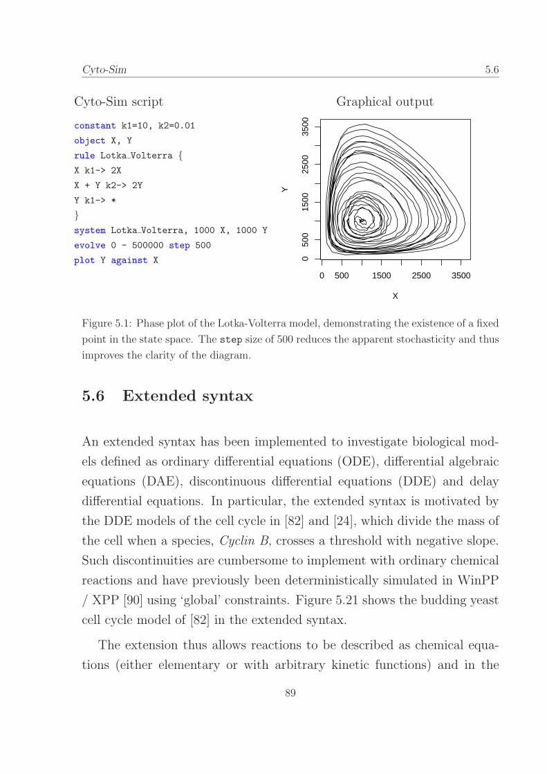
Cyto-Sim 5.6
Cyto-Sim script Graphical output
0 500 1500 2500 3500
050
015
0025
0035
00X
Y
constant k1=10, k2=0.01
object X, Y
rule Lotka Volterra X k1-> 2X
X + Y k2-> 2Y
Y k1-> *
system Lotka Volterra, 1000 X, 1000 Y
evolve 0 - 500000 step 500
plot Y against X
Figure 5.1: Phase plot of the Lotka-Volterra model, demonstrating the existence of a fixed
point in the state space. The step size of 500 reduces the apparent stochasticity and thus
improves the clarity of the diagram.
5.6 Extended syntax
An extended syntax has been implemented to investigate biological mod-
els defined as ordinary differential equations (ODE), differential algebraic
equations (DAE), discontinuous differential equations (DDE) and delay
differential equations. In particular, the extended syntax is motivated by
the DDE models of the cell cycle in [82] and [24], which divide the mass of
the cell when a species, Cyclin B, crosses a threshold with negative slope.
Such discontinuities are cumbersome to implement with ordinary chemical
reactions and have previously been deterministically simulated in WinPP
/ XPP [90] using ‘global’ constraints. Figure 5.21 shows the budding yeast
cell cycle model of [82] in the extended syntax.
The extension thus allows reactions to be described as chemical equa-
tions (either elementary or with arbitrary kinetic functions) and in the
89

5.6 Cyto-Sim
format of differential equations. E.g., the differential equation
dCycBT
dt= k1 − (k2.1 + k2.2Cdh1 + k2.3Cdc20A)CycBT
could be entered as four elementary chemical reactions in the standard
Cyto-Sim syntax:* k1-> CycBT CycBT k2.1-> *
CycBT + Cdh1 k2.2-> Cdh1
CycBT + Cdc20A k2.3-> Cdc20A
or in a single line differential equation in the extended syntax:
CycBT’ = k1 - (k2.1+k2.2*Cdh1+k2.3*Cdc20A)*CycBT
Algebraic equations such as
CycB = (1-2*CKIT/((BB=CycBT+CKIT+Kdiss)+sqrt(BB*BB-4*CycBT*CKIT)))*CycBT*M/beta
may also be included in the simulation script. These equations are evalu-
ated when any of the values appearing on the right hand side of the equa-
tion change. If there is more than one equation that is affected, they are
evaluated in the order they are written in the file. The above example also
illustrates in-line evaluation (i.e., BB=CycBT+CKIT+Kdiss), which is performed
using left-to-right priority.
To control the discontinuities of DDEs, a type of instantaneous reaction
controlled by a predicate has been implemented. E.g., the following two
reactions control when the cell divides in the cell cycle model used in
Chapter 10:div0 [CycB*M/beta<thresh0,M=M/2]-> div1
div1 [CycB*M/beta>thresh1]-> div0
As with the normal chemical paradigm, the reactants (i.e., div0 and div1)
must exist for the reaction to be enabled and when the reaction fires, the
reactants are consumed and the products produced simultaneously. The
difference in this case is that the reaction is also controlled by a comma-
separated list of predicates or expressions interpreted as predicates (zero
90

Cyto-Sim 5.6
being false and values greater than zero being true) within square brackets.
These are evaluated in left-to-right order with short-circuiting.
In the above example div0 and div1 are tokens which indicate the state
of CycB. The initial condition is that div0 exists and div1 does not, hence
only the first reaction can possibly fire. When CycB ∗ M/beta is lower
than the threshold thresh0, the first predicate in the list returns true and
the second one is evaluated. In this case the predicate is an expression
which divides the mass by two and has a resulting value greater than
zero, so the reaction is executed. Note that the short-circuiting prevents
the mass division expression being evaluated more than once. With div0
consumed, only the second reaction is now possible and it will only fire
when CycB ∗M/beta reaches threshold thresh1.
Other features of the extensions include the keyword simulate, which
allow the possibility to run simulations with respect to time rather than
steps.
91

5.7 Cyto-Sim
5.7 Examples
The following subsections contain examples of Cyto-Sim scripts.
5.7.1 Lotka-Volterra Reactions
Possibly the simplest and most well known chemical oscillator is charac-
terised by the Lotka autocatalytic reactions [59] (subsequently and inde-
pendently modelled by Volterra). Figure 5.2 is a model which uses Cyto-
Sim native chemical rules, which assume mass action and therefore require
only a rate to fully specify the kinetics. Figure 5.4 is an equivalent model
using Cyto-Sim Petri net incidence matrix syntax. Figure 5.3 is the corre-
sponding Petri net diagram. Note that due to the limitations of incidence
matrices in describing stoichiometry, it is necessary to explicitly describe
the mass action kinetic laws for transitions t1 and t2. These transitions
have incoming and outgoing arcs incident on the same place, which result
in a zero entry in the matrix. It is therefore necessary to explicitly state
the kinetic dependence. Simulations of the two models are statistically in-
distinguishable and Figure 5.5 is a typical example. Note that this system
of reactions produce neutrally stable oscillations and it has a fixed point
at Y1 = Y2 = 0. Hence, if the simulation is run long enough, this condi-
tion will eventually be met and the simulator will halt because there is no
auto-generation of either Y1 or Y2.
5.7.2 Oregonator
Field and Noyes [29] produced a generalisation of the Belousov-Zhabotinskii
reactions using five steps and three independent intermediate chemical
species, which they called the Oregonator reactions. These demonstrate
limit cycle (i.e. positively stable) oscillations using reactions that require
no more than two reacting molecules (in contrast to the so-called Brusse-
92

Cyto-Sim 5.7
lator [69], which requires reactions involving three reactants). A model of
the Oregonator reactions using Cyto-Sim native rules is shown in Figure
5.6. The Petri net version of the same model is given in Figure 5.8, with a
corresponding Petri net diagram shown in figure 5.7. As with the previous
Petri net model, the kinetics of some of the reactions must be explicitly
defined. A simulation of this model is shown in Figure 5.9.
5.7.3 Noise-Resistant Oscillator
A sophisticated biochemically-inspired oscillator is the noise resistant os-
cillator of [84], represented in Figure 5.10 as a diagram adapted from the
original article. This achieves temporal stability with small numbers of
molecules by virtue of its topology. Figure 5.11 is the model described
using Cyto-Sim’s native chemical syntax. The assumption of mass action
kinetics allows a compact description of each reaction, which require only
the addition of a rate to specify the kinetic behaviour. Figure 5.13 is the
same model given as a Petri net incidence matrix, shown diagrammatically
in Figure 5.12. As with the previous Petri net models, the limitations of
an incidence matrix require that the kinetic laws for some transitions be
explicitly described.
Figure 5.14 is an example simulation of the noise resistant oscillator,
demonstrating the expected periodicity. No explicit units are given in the
model, however rates are assumed to be hours−1 or molecules−1hours−1,
as appropriate. Figure 5.15 shows the simulated effect of switching off the
gene for protein pR. This is achieved in the simulator model by the inclusion
of -1 gR@50000,-1 g_R@50000 in the system statement:
system 1 gA,1 gR,circadian_clock,-1 gR@50000,-1 g_R@50000
This has the effect of deleting gR or g_R at evolution step 50000 (both must
be deleted since it cannot be predicted which of these two states the gene
93

5.7 Cyto-Sim
object X,Y1,Y2,Z
rule lotka volterra
X + Y1 0.0002-> 2Y1 + X
Y1 + Y2 0.01-> 2Y2
Y2 10-> Z
system 100000 X,1000 Y1,1000 Y2,lotka volterra
evolve 0-500000 step 500
plot Y2,Y1
Figure 5.2: Lotka-Volterra reactions using Cyto-Sim native rule syntax.
will be in).
5.7.4 Oscillatory behaviour of NF-κB
The model is given in Figure 5.16 and a typical output plot is given in
Figure 5.18. Very little stochastic noise is evident due to the relatively
large numbers of molecules in the system.
Figure 5.3: Petri net representation of Lotka-Volterra reactions (tokens omitted).
94

Cyto-Sim 5.7
object X,Y1,Y2,Z
petri lotka volterra
X ,Y1,Y2,Z
t1 0 ,1 ,0 ,0 :(0.0002*X*Y1)
t2 0 ,-1,1 ,0 :(0.01*Y1*Y2)
t3 0 ,0 ,-1,1 :10
system 100000 X,1000 Y1,1000 Y2,lotka volterra
evolve 0-500000 step 500
plot Y2,Y1
Figure 5.4: Lotka-Volterra reactions using a Petri net incidence matrix.
Figure 5.5: Typical simulation trace of Lotka-Volterra reactions.
95
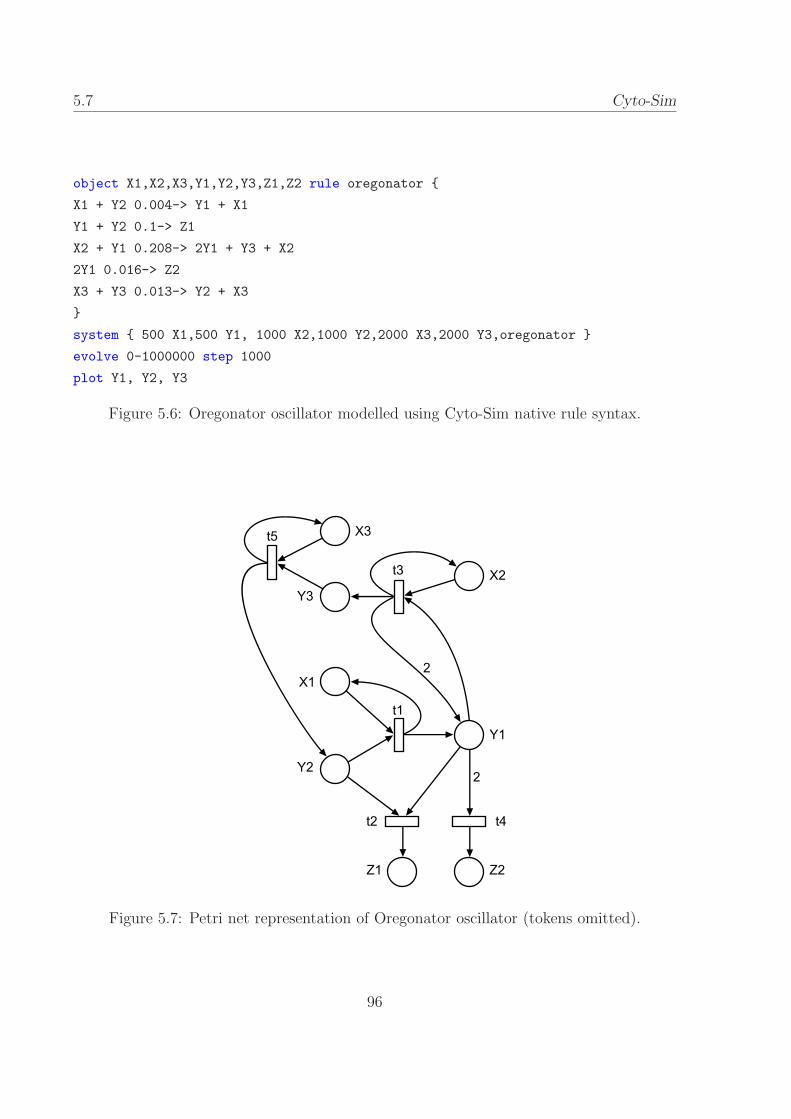
5.7 Cyto-Sim
object X1,X2,X3,Y1,Y2,Y3,Z1,Z2 rule oregonator
X1 + Y2 0.004-> Y1 + X1
Y1 + Y2 0.1-> Z1
X2 + Y1 0.208-> 2Y1 + Y3 + X2
2Y1 0.016-> Z2
X3 + Y3 0.013-> Y2 + X3
system 500 X1,500 Y1, 1000 X2,1000 Y2,2000 X3,2000 Y3,oregonator
evolve 0-1000000 step 1000
plot Y1, Y2, Y3
Figure 5.6: Oregonator oscillator modelled using Cyto-Sim native rule syntax.
Figure 5.7: Petri net representation of Oregonator oscillator (tokens omitted).
96

Cyto-Sim 5.7
object X1,X2,X3,Y1,Y2,Y3,Z1,Z2
petri oregonator
X1,X2,X3,Y1,Y2,Y3,Z1,Z2
t1 0 ,0 ,0 ,1 ,-1,0 ,0 ,0 :(0.004*X1*Y2)
t2 0 ,0 ,0 ,-1,-1,0 ,1 ,0 :0.1
t3 0 ,0 ,0 ,1 ,0 ,1 ,0 ,0 :(0.208*X2*Y1)
t4 0 ,0 ,0 ,-2,0 ,0 ,0 ,1 :0.016
t5 0 ,0 ,0 ,0 ,1 ,-1,0 ,0 :(0.013*X3*Y3)
system 500 X1,500 Y1,1000 X2,1000 Y2,2000 X3,2000 Y3,oregonator
evolve 0-1000000 step 1000
plot Y1, Y2, Y3
Figure 5.8: Oregonator oscillator modelled using a Petri net incidence matrix.
Figure 5.9: Typical simulation trace of Oregonator oscillator.
97

5.7 Cyto-Sim
Figure 5.10: Reaction scheme of noise-resistant oscillator, adapted from [84].
object
IkBa,NF_kB,IkBa_NF_kB,IkBb,IkBb_NF_kB,IkBe,IkBe_NF_kB,IKK,NF_kBn,IkBan,
IkBan_NF_kBn,IkBbn,IkBbn_NF_kBn,IkBen,IkBen_NF_kBn,IkBa_t,IkBb_t,IkBe_t,
IKKIkBa,IKKIkBa_NF_kB,IKKIkBb,IKKIkBb_NF_kB,IKKIkBe,IKKIkBe_NF_kB
rule NFkB // Reaction no.
IkBa + NF_kB 8.30E-7-> IkBa_NF_kB // 1.
IkBa_NF_kB 0.5E-3-> NF_kB + IkBa // 2.
IkBb + NF_kB 8.30E-7-> IkBb_NF_kB // 3.
IkBb_NF_kB 0.5E-3-> NF_kB + IkBb // 4.
IkBe + NF_kB 8.30E-7-> IkBe_NF_kB // 5.
IkBe_NF_kB 0.5E-3-> NF_kB + IkBe // 6.
IKKIkBa + NF_kB 8.30E-7-> IKKIkBa_NF_kB // 7.
IKKIkBa_NF_kB 0.5E-3-> NF_kB + IKKIkBa // 8.
IKKIkBa_NF_kB 2.04E-2-> IKK + NF_kB // 9.
IKKIkBb + NF_kB 8.30E-7-> IKKIkBb_NF_kB // 10.
IKKIkBb_NF_kB 0.5E-3-> NF_kB + IKKIkBb // 11.
IKKIkBb_NF_kB 7.5E-3-> IKK + NF_kB // 12.
IKKIkBe + NF_kB 8.30E-7-> IKKIkBe_NF_kB // 13.
IKKIkBe_NF_kB 0.5E-3-> NF_kB + IKKIkBe // 14.
IKKIkBe_NF_kB 1.1E-2-> IKK + NF_kB // 15.
IkBa_NF_kB 2.25E-5-> NF_kB // 16.
98

Cyto-Sim 5.7
object gA,g A,gR,g R,MA,MR,pA,pR,AR
rule circadian clock
gA 50-> MA + gA
pA + gA 1-> g_A
g_A 500-> MA + g_A
gR 0.01-> MR + gR
g_R 50-> MR + g_R
MA 50-> pA
MR 5-> pR
pA + pR 2-> AR
AR 1-> pR
pA 1-> *
pR 0.2-> *
MA 10-> *
MR 0.5-> *
g_R 100-> pA + gR
pA + gR 1-> g_R
g_A 50-> pA + gA
system 1 gA, 1 gR, circadian clock
evolve 0-150000 step 150
plot pA, pR
Figure 5.11: Noise-resistant oscillator [84] modelled using Cyto-Sim native reaction rules.
99

5.7 Cyto-Sim
Figure 5.12: Petri net representation of the noise-resistant oscillator. Initial tokens shown.
100

Cyto-Sim 5.7
object gA,g A,gR,g R,MA,MR,pA,pR,AR
petri circadian clock
gA,g_A,gR,g_R,MA,MR,pA,pR,AR
t1 0 ,0 ,0 ,0 ,1 ,0 ,0 ,0 ,0 :(50*gA)
t2 -1,1 ,0 ,0 ,0 ,0 ,-1,0 ,0 :1
t3 0 ,0 ,0 ,0 ,1 ,0 ,0 ,0 ,0 :(500*g_A)
t4 0 ,0 ,0 ,0 ,0 ,1 ,0 ,0 ,0 :(0.01*gR)
t5 0 ,0 ,0 ,0 ,0 ,1 ,0 ,0 ,0 :(50*g_R)
t6 0 ,0 ,0 ,0 ,-1,0 ,1 ,0 ,0 :50
t7 0 ,0 ,0 ,0 ,0 ,-1,0 ,1 ,0 :5
t8 0 ,0 ,0 ,0 ,0 ,0 ,-1,-1,1 :2
t9 0 ,0 ,0 ,0 ,0 ,0 ,0 ,1 ,-1 :1
t10 0 ,0 ,0 ,0 ,0 ,0 ,-1,0 ,0 :1
t11 0 ,0 ,0 ,0 ,0 ,0 ,0 ,-1,0 :0.2
t12 0 ,0 ,0 ,0 ,-1,0 ,0 ,0 ,0 :10
t13 0 ,0 ,0 ,0 ,0 ,-1,0 ,0 ,0 :0.5
t14 0 ,0 ,1 ,-1 ,0 ,0 ,1 ,0 ,0 :100
t15 0 ,0 ,-1,1 ,0 ,0 ,-1,0 ,0 :1
t16 1 ,-1 ,0 ,0 ,0 ,0 ,1 ,0 ,0 :50
system 1 gA, 1 gR, circadian clock
evolve 0-150000 step 150
plot pA, pR
Figure 5.13: Noise-resistant oscillator modelled using a Petri net incidence matrix.
101

5.7 Cyto-Sim
Figure 5.14: Typical single simulation trace of the noise-resistant oscillator.
Figure 5.15: Typical single simulation trace of switching off the gene for pR in the noise-
resistant oscillator.
Figure 5.16: (below) Model demonstrating oscillatory behaviour in NF-κB [47].
102

Cyto-Sim 5.7
IkBb_NF_kB 2.25E-5-> NF_kB // 17.
IkBe_NF_kB 2.25E-5-> NF_kB // 18.
NF_kB 0.9E-1-> NF_kBn // 19.
NF_kBn 0.8E-4-> NF_kB // 20.
IkBan + NF_kBn 8.30E-7-> IkBan_NF_kBn // 21.
IkBan_NF_kBn 0.5E-3-> NF_kBn + IkBan // 22.
IkBbn + NF_kBn 8.30E-7-> IkBbn_NF_kBn // 23.
IkBbn_NF_kBn 0.5E-3-> NF_kBn + IkBbn // 24.
IkBen + NF_kBn 8.30E-7-> IkBen_NF_kBn // 25.
IkBen_NF_kBn 0.5E-3-> NF_kBn + IkBen // 26.
* 0.927-> IkBa_t // 27.
NF_kBn + NF_kBn 2.74E-8*2-> IkBa_t + NF_kBn + NF_kBn // 28.
IkBa_t 2.8E-4-> * // 29.
* 0.107-> IkBb_t // 30.
IkBb_t 2.8E-4-> * // 31.
* 0.0765-> IkBe_t // 32.
IkBe_t 2.8E-4-> * // 33.
IKK + IkBa 3.74E-08-> IKKIkBa // 34.
IKKIkBa 1.25E-3-> IKK + IkBa // 35.
IkBa_t 4.08E-3-> IkBa + IkBa_t // 36.
IkBa 1.13E-4-> * // 37.
IkBa 3.0E-4-> IkBan // 38.
IkBan 2.0E-4-> IkBa // 39.
IKK + IkBb 9.96E-09-> IKKIkBb // 40.
IKKIkBb 1.75E-3-> IKK + IkBb // 41.
IkBb_t 4.08E-3-> IkBb + IkBb_t // 42.
IkBb 1.13E-4-> * // 43.
IkBb 1.5E-4-> IkBbn // 44.
IkBbn 1.0E-4-> IkBb // 45.
IKK + IkBe 1.49E-08-> IKKIkBe // 46.
IKKIkBe 1.75E-3-> IKK + IkBe // 47.
IkBe_t 4.08E-3-> IkBe + IkBe_t // 48.
IkBe 1.13E-4-> * // 49.
IkBe 1.5E-4-> IkBen // 50.
IkBen 1.0E-4-> IkBe // 51.
IKK + IkBa_NF_kB 3.07E-7-> IKKIkBa_NF_kB // 52.
IKKIkBa_NF_kB 1.25E-3-> IKK + IkBa_NF_kB // 53.
IkBan_NF_kBn 1.38E-2-> IkBa_NF_kB // 54.
103
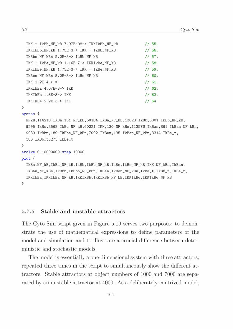
5.7 Cyto-Sim
IKK + IkBb_NF_kB 7.97E-08-> IKKIkBb_NF_kB // 55.
IKKIkBb_NF_kB 1.75E-3-> IKK + IkBb_NF_kB // 56.
IkBbn_NF_kBn 5.2E-3-> IkBb_NF_kB // 57.
IKK + IkBe_NF_kB 1.16E-7-> IKKIkBe_NF_kB // 58.
IKKIkBe_NF_kB 1.75E-3-> IKK + IkBe_NF_kB // 59.
IkBen_NF_kBn 5.2E-3-> IkBe_NF_kB // 60.
IKK 1.2E-4-> * // 61.
IKKIkBa 4.07E-3-> IKK // 62.
IKKIkBb 1.5E-3-> IKK // 63.
IKKIkBe 2.2E-3-> IKK // 64.
system
NFkB,114218 IkBa,151 NF_kB,50184 IkBa_NF_kB,13028 IkBb,5001 IkBb_NF_kB,
9295 IkBe,3568 IkBe_NF_kB,60221 IKK,130 NF_kBn,113576 IkBan,861 IkBan_NF_kBn,
9939 IkBbn,189 IkBbn_NF_kBn,7092 IkBen,135 IkBen_NF_kBn,3314 IkBa_t,
383 IkBb_t,273 IkBe_t
evolve 0-10000000 step 10000
plot
IkBa,NF_kB,IkBa_NF_kB,IkBb,IkBb_NF_kB,IkBe,IkBe_NF_kB,IKK,NF_kBn,IkBan,
IkBan_NF_kBn,IkBbn,IkBbn_NF_kBn,IkBen,IkBen_NF_kBn,IkBa_t,IkBb_t,IkBe_t,
IKKIkBa,IKKIkBa_NF_kB,IKKIkBb,IKKIkBb_NF_kB,IKKIkBe,IKKIkBe_NF_kB
5.7.5 Stable and unstable attractors
The Cyto-Sim script given in Figure 5.19 serves two purposes: to demon-
strate the use of mathematical expressions to define parameters of the
model and simulation and to illustrate a crucial difference between deter-
ministic and stochastic models.
The model is essentially a one-dimensional system with three attractors,
repeated three times in the script to simultaneously show the different at-
tractors. Stable attractors at object numbers of 1000 and 7000 are sepa-
rated by an unstable attractor at 4000. As a deliberately contrived model,
104

Cyto-Sim 5.7
µ Dependent reactions Dµ |Dµ| µ Dependent reactions Dµ |Dµ|
1. 1,2,3,5,7,10,13,16,19,34,37,38,52 13 33. 33,48 2
2. ,1,2,3,5,7,10,13,16,19,34,37,38,52 13 34. 1,7,34,35,37,38,40,46,52,55,58,61,62 13
3. 1,3,4,5,7,10,13,17,19,40,43,44,55 13 35. 1,7,34,35,37,38,40,46,52,55,58,61,62 13
4. 1,3,4,5,7,10,13,17,19,40,43,44,55 13 36. 1,34,37,38 4
5. 1,3,5,6,7,10,13,18,19,46,49,50,58 13 37. 1,34,37,38 4
6. 1,3,5,6,7,10,13,18,19,46,49,50,58 13 38. 1,21,34,37,38,39 6
7. 1,3,5,7,8,9,10,13,19,35,53,62 12 39. 1,21,34,37,38,39 6
8. 1,3,5,7,8,9,10,13,19,35,53,62 12 40. 3,10,34,40,41,43,44,46,52,55,58,61,63 13
9. 1,3,5,7,8,9,10,13,19,34,40,46,52,53,55,58,61 17 41. 3,10,34,40,41,43,44,46,52,55,58,61,63 13
10. 1,3,5,7,10,11,12,13,19,41,56,63 12 42. 3,40,43,44 4
11. 1,3,5,7,10,11,12,13,19,41,56,63 12 43. 3,40,43,44 4
12. 1,3,5,7,10,11,12,13,19,34,40,46,52,55,56,58,61 17 44. 3,23,40,43,44,45 6
13. 1,3,5,7,10,13,14,15,19,47,59,64 12 45. 3,23,40,43,44,45 6
14. 1,3,5,7,10,13,14,15,19,47,59,64 12 46. 5,13,34,40,46,47,49,50,52,55,58,61,64 13
15. 1,3,5,7,10,13,14,15,19,34,40,46,52,55,58,59,61 17 47. 5,13,34,40,46,47,49,50,52,55,58,61,64 13
16. 1,2,3,5,7,10,13,16,19,52 10 48. 5,46,49,50 4
17. 1,3,4,5,7,10,13,17,19,55 10 49. 5,46,49,50 4
18. 1,3,5,6,7,10,13,18,19,58 10 50. 5,25,46,49,50,51 6
19. 1,3,5,7,10,13,19,20,21,23,25,28 12 51. 5,25,46,49,50,51 6
20. 1,3,5,7,10,13,19,20,21,23,25,28 12 52. 2,8,9,16,34,40,46,52,53,55,58,61 12
21. 20,21,22,23,25,28,39,54 8 53. 2,8,9,16,34,40,46,52,53,55,58,61 12
22. 20,21,22,23,25,28,39,54 8 54. 2,16,22,52,54 5
23. 20,21,23,24,25,28,45,57 8 55. 4,11,12,17,34,40,46,52,55,56,58,61 12
24. 20,21,23,24,25,28,45,57 8 56. 4,11,12,17,34,40,46,52,55,56,58,61 12
25. 20,21,23,25,26,28,51,60 8 57. 4,17,24,55,57 5
26. 20,21,23,25,26,28,51,60 8 58. 6,14,15,18,34,40,46,52,55,58,59,61 12
27. 29,36 2 59. 6,14,15,18,34,40,46,52,55,58,59,61 12
28. 29,36 2 60. 6,18,26,58,60 5
29. 29,36 2 61. 34,40,46,52,55,58,61 7
30. 31,42 2 62. 7,34,35,40,46,52,55,58,61,62 10
31. 31,42 2 63. 10,34,40,41,46,52,55,58,61,63 10
32. 33,48 2 64. 13,34,40,46,47,52,55,58,61,64 10
Figure 5.17: Reaction dependency of NF-κB model of Figure 5.16. Dµ is the set of
reactions whose propensity is affected by reaction µ. Mean |Dµ| = 9.05.
105
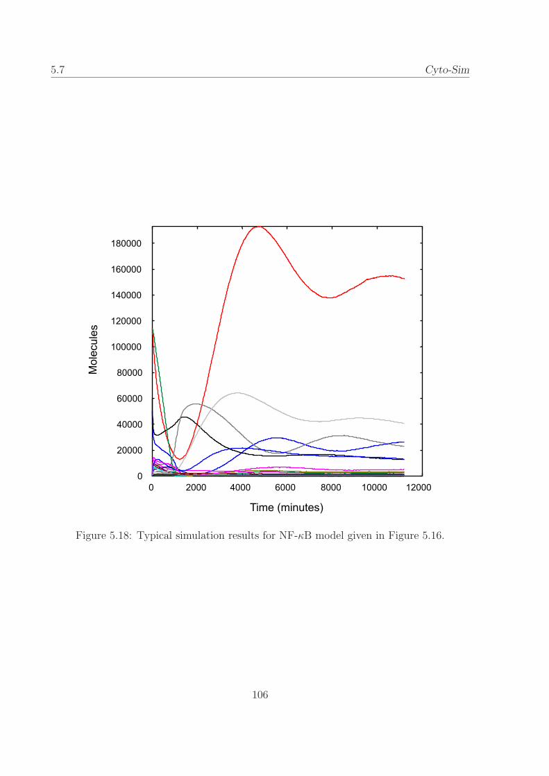
5.7 Cyto-Sim
Figure 5.18: Typical simulation results for NF-κB model given in Figure 5.16.
106

Cyto-Sim 5.7
these values can be set precisely using constants x1, x2 and x3, respectively.
With initial value X = 8000, X tends to the stable attractor at X = 7000.
With initial value Z = 0, Z tends to the stable attractor at Z = 1000. With
initial value Y = 4000, Y is placed directly on the unstable attractor and
randomly tends to one of the stable attractors. This is illustrated in Figure
5.20. This behaviour is in contrast to that of a deterministic simulation
of the same system using ordinary differential equations (ODEs), where Y
will tend to remain on the unstable attractor. This is because in the ODE
context the ‘forces’ on Y cancel to exactly zero and remain so.
107

5.7 Cyto-Sim
constant alpha=1000000,x1=1000,x2=7*x1,x3=(x1+x2)/2
constant k=(x3*x3*(x3/3-x1)-x1*x1*(x1/3-x3))/(x3-x1)
constant a=x3*x3-k,c=x3*(x3*x3/3-k)
object X,Y,Z
rule Xattractor
X a/alpha-> *
c/alpha-> X
X + X + X 2/alpha-> X + X
X + X 2*x3/alpha-> X + X + X
rule Yattractor
Y a/alpha-> *
c/alpha-> Y
Y + Y + Y 2/alpha-> Y + Y
Y + Y 2*x3/alpha-> Y + Y + Y
rule Zattractor
Z a/alpha-> *
c/alpha-> Z
Z + Z + Z 2/alpha> Z + Z
Z + Z 2*x3/alpha-> Z + Z + Z
system Xattractor, Yattractor, Zattractor, 8*x1 X, x3 Y, 0 Z
evolve 0-2000*x1 step x1/10
plot X,Y,Z
Figure 5.19: Cyto-Sim script to demonstrate stable and unstable attractors.
108

Cyto-Sim 5.7
Figure 5.20: Two Cyto-Sim simulation traces showing how various initial conditions tend
to stable attractors (X: upper trace in red, Z: lower trace in blue) and randomly away from
an unstable attractor (Y: middle trace in green).
109

5.7 Cyto-Sim
constant alpha=424,beta=1000,thresh0=0.1*alpha,thresh1=0.2*alpha
constant k1=0.04*alpha,k2.1=0.04,k2.2=1/alpha,k2.3=1/alpha
constant k3.1=alpha,k3.2=10,k4.1=2,k4=35,k5.1=0.005*alpha,k5.2=0.2*alpha,k6=0.1
constant J3=0.04*alpha,J4=0.04*alpha,J5=0.3*alpha,k7=1,k8=0.5,J7=0.001*alpha
constant J8=0.001*alpha,Mad1=alpha,k9=0.1/alpha,k10=0.02,k11=alpha,k12.1=0.2
constant k12.2=50/alpha,k12.3=100/alpha,Kdiss=0.001*alpha,k13.1=0*alpha,k13.2=1,k14=1
constant k15.1=1.5*alpha/beta,k15.2=0.05,k16.1=alpha,k16.2=3,J15=0.01*alpha
constant J16=0.01*alpha,mu=0.005,Mstar=10*beta
species CycBT=alpha,Cdh1,Cdc20T=alpha,Cdc20A,IE,CKIT,SK,TF,M=beta,BB,CycB,div0=1,div1
// Algebraic equation
CycB = (1-2*CKIT/((BB=CycBT+CKIT+Kdiss)+sqrt(BB*BB-4*CycBT*CKIT)))*CycBT*M/beta
div0 [CycB*M/beta<thresh0,M=M/2]-> div1 // Mass division control
div1 [CycB*M/beta>thresh1]-> div0 // using predicate reactions
// Creation & consumption reactions with summed rate functions
* k1-> CycBT
CycBT ((k2.1+k2.2*Cdh1+k2.3*Cdc20A)*CycBT)-> *
* ((k3.1+k3.2*Cdc20A)*(alpha-Cdh1)/(J3+alpha-Cdh1))-> Cdh1
Cdh1 ((k4.1*SK+k4*CycB)*Cdh1/(J4+Cdh1))-> *
* (k5.1+k5.2*CycB^4/(J5^4+CycB^4))-> Cdc20T
Cdc20T (k6*Cdc20T)-> *
* (k7*IE*(Cdc20T-Cdc20A)/(J7+Cdc20T-Cdc20A))-> Cdc20A
Cdc20A (k8*Mad1*Cdc20A/(J8+Cdc20A)+k6*Cdc20A)-> *
* (k9*(alpha-IE)*CycB)-> IE
IE (k10*IE)-> *
* k11-> CKIT
CKIT ((k12.1+k12.2*SK+k12.3*CycB)*CKIT)-> *
* (k13.1+k13.2*TF)-> SK
SK k14-> *
* ((k15.1*M+k15.2*SK)*(alpha-TF)/(J15+alpha-TF))-> TF
TF ((k16.1+k16.2*CycB)*TF/(J16+TF))-> *
* (mu*M*(1-M/Mstar))-> M
simulate 1000 step 0.5 // Simulation specification in terms of time
Figure 5.21: Budding yeast cell cycle model of [82] expressed in extended syntax (see
Section 5.6). The terms of the original ODEs have been divided into stochastic creation
and consumption reactions.
110

Chapter 6
From Single Cells to Tissues:
Colonies of Synchronizing Agents
The work presented in this chapter was originally published in
M. Cavaliere, R. Mardare and S. Sedwards (2007) Colonies of Synchronizing Agents: An Ab-
stract Model of Intracellular and Intercellular Processes, Proceedings of the International Work-
shop on Automata for Cellular and Molecular Computing, Budapest.
and
M. Cavaliere, R. Mardare and S. Sedwards (2008) A multiset-based model of synchronizing
agents: Computability and robustness, Theoretical Computer Science, 391:3, 216–238.
The models presented in Chapters 3 – 5 have considered a static and finite
membrane structure. In order to now study systems whose structure may
change or emerge, a modelling framework and computational paradigm is
presented called Colonies of Synchronizing Agents (CSA), inspired by the
intracellular and intercellular mechanisms in biological tissues.
The model is based on a multiset of agents in a common environment.
Each agent has a local state stored in the form of a multiset of atomic
objects, which is updated by global multiset rewriting rules either inde-
pendently or synchronously with another agent.
The model is first defined and its computational power is then stud-
111

6.1 Colonies of Synchronizing Agents
ied, considering trade-offs between internal rewriting (intracellular mech-
anisms) and synchronization between agents (intercellular mechanisms).
The dynamic properties of CSAs are also investigated, including behavioural
robustness (ability to generate a core behaviour despite agent loss or rule
failure) and safety of synchronization (ability of an agent to synchronise
with some other agent whenever needed).
6.1 Introduction and motivations
Inspired by intracellular and intercellular mechanisms in biological tissues,
an abstract distributed model of computation called Colonies of Synchro-
nizing Agents (in short CSA) is presented and investigated. The intention
is to create a framework to model, analyse and simulate biological tissues
in the context of formal language and multiset rewriting.
The model is based on a population of agents (e.g., corresponding to cells
or molecules) in a common environment, able to modify their contents and
to synchronise with other agents in the same environment. Each agent has
a contents represented by a multiset of atomic objects (e.g., corresponding
to chemical compounds or the characteristics of individual molecules) with
some of the objects classified as terminals (e.g., corresponding to chemi-
cals or properties visible to an external observer). The agents’ contents
may be modified by means of multiset rewriting rules (called evolution
rules), which may mimic chemical or other types of intracellular mecha-
nisms. Moreover, the agents can influence each other by synchronously
changing their contents using pairwise synchronization rules. This models,
in a deliberately abstract way, the various intercellular mechanisms present
in biological tissues (e.g., signalling mechanisms that cells and biological
systems use). All rules are global, so all agents obey the same rules: the
only feature that may distinguish the agents is their contents.
112
Colonies of Synchronizing Agents 6.1
Hence, a CSA is essentially a multiset of mutisets, acted upon by mul-
tiset rewriting rules.
In this chapter CSAs are considered as generative computing devices and
various trade-offs between the power of the evolution rules and the power of
the synchronizing rules are considered. CSAs are considered working in a
maximally parallel way (all agents are updated synchronously), modelling
the idea that if something can happen then it must happen. However,
from both a biological and a mathematical point of view, it is also useful
to investigate systems where the update of the agents is not obligatory
(i.e., not synchronous). It is shown that the computational power of max-
imal parallel and asynchronous CSAs can range from that of finite sets
of vectors to that of Turing machines, by varying the power of the evolu-
tion and synchronization rules. Moreover, an intermediate class of CSAs,
equivalent to partially blind counter machines (hence, not universal [42]),
is investigated.
Having investigated the computational power of CSAs, the robustness of
colonies is studied by considering their ability to generate core behaviours
despite the failure (i.e., removal) of agents or of rules. It is shown that
for an arbitrary CSA, robustness cannot be decided but that it is possible
to individuate classes of (non-trivial) CSAs where this property can be
efficiently decided.
The final part of the chapter is concerned with dynamic properties of
CSAs in regard to the applications of the rules.
For this reason, a decidable temporal logic is provided to specify and
investigate dynamic properties of CSAs. For instance, it is shown that
the proposed logic can be used to specify and then check whether or not
in a CSA an agent has the ability to apply a synchronization whenever
it needs: CSAs for which such a property is true are described safe on
synchronization of rules. This models, in an abstract way, the ability of a
113

6.1 Colonies of Synchronizing Agents
cell to use an intercellular mechanism whenever it needs.
CSAs are computational devices that have features inspired by many
different models. In particular, they have similarities (and significant dif-
ferences) with other models inspired by cell-tissues and investigated in the
area of membrane computing. Specifically, CSAs can be considered a gen-
eralization of P colonies [52], which is also based on interacting agents but
has agents with limited contents (two objects) which can only change their
contents using very restricted rewriting rules (following an earlier defini-
tion of an agent in formal language theory ([51]). In the case of CSAs, in
order to be more general, the rewriting rules employed by an agent and the
contents of an agent can be arbitrarily complex. Moreover, in P colonies
objects can be introduced into the agent from an external environment
(with unbounded copies of a given object) and the objects present in an
agent may only be transferred to another agent by means of the common
environment; no direct communication between agents is allowed (as is the
case in CSAs).
CSAs also have similarities with population P systems [6], a class of
tissue P systems [61], and in particular with EC tissue P systems [7],
where evolution (rewriting) is combined with communication. Cells (i.e.,
agents) can change their contents by means of (non-cooperative) rewriting
rules and hence different types of agents can have different sets of rules.
It is also possible to move objects between the agents using ‘bonds’ and
agents may also communicate with an environment that has unbounded
resources. Computation is generally implemented in two different phases:
local rewriting plus bond making rules, applied in an alternate manner.
The main differences with these computing devices and the model described
here are that CSAs do not have explicit bonds (edges) between agents
(in a sense agents are linked by a complete graph), rewriting in CSAs
is arbitrarily complex (i.e., it can be cooperative) for both evolution and
114

Colonies of Synchronizing Agents 6.2
synchronization rules, and CSA agents do not have explicit types: rules
are global and only the agents’ contents differentiate them. This latter
characteristic makes CSAa similar to the model of self-assembly of graphs
presented in [5], however in that case (i) a graph is constructed from an
initial seed using multiset-based aggregation rules to enlarge the structure,
(ii) there is no internal rewriting of the agent contents and (iii) there is
no synchronization between the agents.
CSAs are also distinct from cellular automata [48], where cells exist on a
regular grid, where each cell has a finite number of possible states and where
cells interact with a defined neighbourhood. In the case of CSAs, as a result
of the multiset-based contents and because of the general rewriting rules,
the possible different internal states of a cell may be infinite. Although
the initial definition does not include an explicit description of space, the
proposed extensions include agents located at arbitrary positions and with
the potential to interact with any other agent in the system.
6.2 Preliminaries
In this section, certain preliminary definitions and descriptions are given
which have specific relevance to Colonies of Synchronizing Agents.
The following recalls some definitions and results from specific variants
of membrane systems which are used in the proofs of this chapter. Readers
not interested in the proofs can therefore skip this section.
Definition 6.2.1 ([71]) A P system with symbol-objects and of degree
m ≥ 1 is defined as a construct
Π = (V, T, µ, w1, . . . , wm, R1, . . . , Rm, i0)
where
115

6.2 Colonies of Synchronizing Agents
• V is an alphabet and its elements are called objects; T ⊆ V is a
terminal alphabet;
• µ is a membrane structure consisting of m membranes arranged in an
hierarchical tree structure; the membranes (and hence the regions that
they delimit) are injectively labelled with 1, 2, . . . ,m;
• wi, 1 ≤ i ≤ m, are strings that represent multisets over V associated
to regions 1, 2, . . . ,m of µ;
• Ri, 1 ≤ i ≤ m, are finite sets of evolution rules over V ; Ri is associ-
ated to region i of µ; an evolution rule is of the form u→ v, where u
is a string over V and v is a string over ahere, aout | a ∈ V ∪ ainj|
a ∈ V, 1 ≤ j ≤ m.
• i0 ∈ 0, 1, 2, . . . ,m; if i0 ∈ 1, . . . ,m then it is the label the mem-
brane that encloses the output region; if i0 = 0 then the output region
is the environment.
For any evolution rule u→ v the length of u is called the radius of the rule
and the symbols here, out, inj, 1 ≤ j ≤ m, are called target indications.
By virtue of the radius of the evolution rules it is possible to distinguish
cooperative rules (if the radius is greater than one) and non-cooperative
rules (otherwise).
The initial configuration of the system Π comprises the structure µ and
the multisets represented by the strings wi, 1 ≤ i ≤ m. In general, a
configuration of the system is the m-tuple of multisets of objects present
at any time in the m regions of the system.
An occurrence γr of the rule r : u → v ∈ Ri, i ∈ 1, · · · ,m can be
applied in region i by assigning to γr a multiset of objects u taken from
the multiset of objects present in region i.
116
Colonies of Synchronizing Agents 6.2
The application of an instance of the evolution rule u → v in a region
i means to remove the multiset of objects u from the multiset of objects
present in region i and to add the multiset v to the multisets of objects
present in the adjacent regions, according to the target indications associ-
ated to each occurrence of the objects in v. In particular, if v contains an
occurrence with target indication here, then the occurrence will be placed
in the region i, where the rule has been applied. If v contains an occurrence
with target indication out, then the occurrence will be moved to the region
immediately outside the region i (this can be the environment if the region
where the rule has been applied is the outermost or skin membrane). If
v contains an occurrence with target indication inj then the occurrence
is moved from the region i and placed in region j (this can be done only
if region j is directly contained by region i; otherwise the evolution rule
u→ v cannot be applied).
A transition between configurations is executed using the evolution rules
in a non-deterministic maximally parallel manner at each step, in each re-
gion (it is supposed that a global clock exists, marking the instant of each
step for the whole system). This means that occurrences of the objects are
assigned to occurrences of the rules in such a way that, after the assign-
ment is made, there are insufficient occurrences of the objects for further
occurrences of any of the rules to be applied. This maximal assignment is
performed simultaneously in every region of the system at each step. If an
occurrence of an object can be assigned to more than one occurrence of
the rules then the assignment is chosen in a non-deterministic way.
A sequence of transitions between configurations of a system is called
a evolution; an evolution is a successful computation (or simply a compu-
tation) if and only if it starts from the initial configuration and halts, i.e.,
it reaches a halting configuration where no occurrence of any rule can be
applied in any region.
117

6.2 Colonies of Synchronizing Agents
The output of a computation is defined as the number of occurrences of
objects from T present in the output region in the halting configuration of
Π; the set of numbers computed (or generated) in this way by the system
Π, considering any computation, is denoted by N(Π).
It is possible to consider as the result of a computation the vector of
numbers representing the multiplicities of the occurrences of objects from
T present in the output region in the halting configuration. In this case
PsT (Π) denotes the set of vectors of numbers generated by Π, considering
all the computations.
NOPm(α, tar) and PsOPm(α, tar) denote the family of sets of the form
N(Π) and Ps(Π), respectively, generated by symbol-objects P systems
of degree at most m ≥ 1 (if the degree is not bounded the subscript m
becomes ∗), using evolution rules of the type α.
α may be given as α = coo, indicating that the systems considered use
cooperative evolution rules, and α = ncoo, indicating that the systems use
only non-cooperative rules.
Moreover, the symbol tar indicates that the communication between
the membranes (and hence the regions) is made using the target indication
inj in the way previously specified. If the degree of the system is 1 (only
one membrane is present) then the only possible target indications that
can be used are here and out and in such case the notation is NOP1(α)
and PsOP1(α), respectively.
The following results are known (see, e.g., [71]).
Theorem 6.2.1
• PsOP∗(ncoo, tar) = PsOP1(ncoo) = PsCF .
• PsOP∗(coo, tar) = PsOPm(coo, tar) = PsRE for all m ≥ 1.
The definition and main results of evolution-communication P systems
[16] are recalled here. This joins two basic models of membrane sys-
118

Colonies of Synchronizing Agents 6.2
tems; that with evolution rules and symbol-objects and that with sym-
port/antiport rules (see, e.g, [71]).
Definition 6.2.2 An evolution-communication P system (in short, an EC
P system) of degree m ≥ 1, is defined as
Π = (V, µ, w1, w2, . . . , wm, R1, . . . , Rm, R′1, . . . , R
′m, i0)
where:
• V, µ, i0 and wi, 1 ≤ i ≤ m as in Definition 6.2.1;
• Ri, 1 ≤ i ≤ m, are finite sets of simple evolution rules over V ; Ri
is associated with the region i of µ; a simple evolution rule is of the
form u→ v, where u ∈ V + and v ∈ V ∗; hence, a simple evolution rule
is an evolution rule as in P systems with symbol-objects, but with no
target indications (in other words it uses an implicit ‘here’ for target
indications);
• R′i, 1 ≤ i ≤ m, are finite sets of symport rules over V of the form
(x, in), (y, out) and of antiport rules (x, in; y, out) with x, y ∈ V +;
R′i is associated with membrane i of µ. For a symport rule (x, in)
or (x, out), |x| is called the weight of the rule. For an antiport rule
(x, in; y, out) the weight is the max|x|, |y|.
In an EC P system a configuration is represented by the membrane
structure µ and by the m-tuple of multisets of objects present in the m
regions of the system.
In particular, the initial configuration comprises the system of mem-
branes µ and the multisets represented by the strings wi, 1 ≤ i ≤ m.
Occurrences of evolution rules are applied as in P systems with symbol-
objects.
119

6.2 Colonies of Synchronizing Agents
An occurrence γ of a symport rule (x, in) ∈ R′i ((x, out) ∈ R′i) can be
applied to membrane i by assigning to γ the occurrences of the objects in
x taken from the region surrounding region i (taken from region i, respec-
tively).
The application of an instance of the symport rule (x, in) to membrane
i consists of moving the occurrences of the objects in x from the region (or
from the environment) surrounding the region i to region i . If an instance
of the symport rule (x, out) is applied to membrane i, the occurrences of the
objects in x are moved from region i to the region (or to the environment)
that surrounds region i.
An occurrence γ of the antiport rule (x, in; y, out) ∈ R′i can be applied
to membrane i by assigning to γ the occurrences of the objects in x taken
from region i and the occurrences of the objects in y taken from the region
surrounding region i.
If an instance of the antiport rule (x, in; y, out) is applied to membrane
i, the occurrences of the objects in x pass into the region i from the region
surrounding it, while, at the same time, the occurrences of the objects in
y move from the surrounding region to region i.
A transition between configurations is governed by the mixed applica-
tion of occurrences of the evolution rules and of the symport/antiport rules.
Instances of the rules from Ri are applied to occurrences of objects in re-
gion i while the application of the instances of rules from R′i govern the
communication of the occurrences of objects through membrane i. There
is no distinction drawn between evolution rules and communication rules
(mixed approach): they are applied in the non-deterministic maximally
parallel manner, described above.
The system starts from the initial configuration and passes from one
configuration to another by applying the above described transitions: this
sequence of transitions is called an evolution of the system. The system
120

Colonies of Synchronizing Agents 6.3
halts when it reaches a halting configuration, i.e., a configuration where no
occurrence of any rule (evolution rules or symport/antiport rules) can be
applied in any region of Π.
In this case the evolution is called a successful computation of Π (or
simply a computation of Π) and the number of occurrences of objects
contained in the output region i0 in the halting configuration is the result
of the computation. The set of numbers computed (or generated) in this
way by the system Π, considering any possible computation of Π, is denoted
by N(Π).
It is also possible to consider as a result of the computation the vector
of numbers representing the multiplicities of the occurrences of the objects
contained in the output region in the halting configuration. In this case
Ps(Π) denotes the set of vectors generated by Π, considering all computa-
tions.
The notation NECPm(i, j, α), α ∈ ncoo, coo, and PsECPm(i, j, α),
α ∈ ncoo, coo, is used to denote the family of sets of numbers and the
family of sets of vectors of numbers, respectively, generated by EC P sys-
tems with at most m membranes (as usual, m = ∗ if such a number is
unbounded), using symport rules of weight at most i, antiport rules of
weight at most j and simple evolution rules that can be cooperative (coo)
or non-cooperative (ncoo).
The following results are known (see, e.g, [16, 3]).
Theorem 6.2.2 • NECP1(1, 0, ncoo) = NCF .
• PsECP1(1, 0, ncoo) = PsCF .
• NECP2(1, 1, ncoo) = NRE.
• PsECP2(1, 1, ncoo) = PsRE.
121

6.3 Colonies of Synchronizing Agents
6.3 Colonies of Synchronizing Agents
In this section the notions of colonies and agents discussed in the Intro-
duction are formally defined.
A Colony of Synchronizing Agents (a CSA) of degree m ≥ 1 is a con-
struct Π = (A, T, C,R) with the components having the following meaning:
• A is a finite alphabet of symbols (its elements are called objects).
T ⊆ A is the alphabet of terminal objects.
• An agent over A is a multiset over the alphabet A (an agent can be
represented by a string w ∈ A∗, since A is finite). C is the initial
configuration of Π and it is a multiset over the set of all possible
agents over A (with card(C) = m) .
Using the notation presented in Chapter 2, C ∈ Mm(H) with H =
M(A).
• R is a finite set of rules over A.
There are evolution rules of type u→ v, with u ∈ A+ and v ∈ A∗.
An instance γ of an evolution rule r : u → v can be applied to an
occurrence ow of agent w by taking a multiset of objects u from ow
(hence, it is required that u ⊆ w) and assigning it to γ (i.e., assigning
the occurrences of the objects in the taken multiset to γ).
The application of an instance of rule r to the occurrence ow of the
agent w consists of removing from ow the multiset u and then adding
v to the resulting multiset.
An evolution rule u → v is said to be cooperative (in short, cooe) if
|u| > 1, non-cooperative (ncooe) if |u| = 1 and unary (une) if |v| ≤|u| = 1.
122

Colonies of Synchronizing Agents 6.3
There are synchronization rules of the type 〈u, v〉 → 〈u′, v′〉 with uv ∈A+ and u′, v′ ∈ A∗.An instance γ of a synchronization rule r : 〈u, v〉 → 〈u′, v′〉 can be
applied to the pair of occurrences ow and ow′ of, respectively, agents
w and w′ by: (i) taking from ow a multiset of objects u and assigning
it to γ; (ii) taking from ow′ a multiset of objects v and assigning it to
γ (hence, it is required that u ⊆ w and v ⊆ w′).
The application of an instance of rule r to the occurrences ow and ow′
consists of: removing the multiset u from ow and then adding u′ to the
resulting multiset; removing the multiset v from ow′ and then adding
v′ to the resulting multiset.
Synchronization rules can be considered as matrices of two rules used
simultaneously.
A synchronization rule 〈u, v〉 → 〈u′, v′〉 is said to be cooperative (coos)
if |u| > 1 or |v| > 1, non-cooperative (ncoos) if |u| = 1 and |v| = 1,
unary (uns) if |u′| ≤ |u| = 1 and |v′| ≤ |v| = 1.
A configuration of a CSA, Π, consists of the occurrences of the agents
present in the system at a given time (the existence of a global clock which
marks the passage of units of time is assumed).
C(Π) denotes the set of all possible configurations of Π. Therefore, using
the notation presented in the Chapter 2, C(Π) is exactly Mm(H) with
H = M(A).
A transition from an arbitrary configuration c of Π to the next lasts
exactly one time unit and can be obtained in two different modes.
Maximally-parallel mode (in short mp): A maximally-parallel transition
of Π (in short, an mp-transition) is obtained by applying the rules in the
set R to the agents present in the configuration c in a maximally parallel
and non-deterministic way. This means that for each occurrence ow of
123

6.3 Colonies of Synchronizing Agents
an agent w and each pair of occurrences ow′ and ow′′ of agents w′ and w′′
present in the configuration c, the occurrences of the objects present in ow
(ow′, ow′′) are assigned to instances of the evolution (synchronization, resp.)
rules, the occurrences of the agents, the occurrences of the objects and the
instances of the rules chosen in a non-deterministic way but respecting the
following condition. After the assignment of the occurrences of the objects
to the instances of the rules is done there is no instance of any rule that can
be applied by assigning the (still) unassigned occurrences of the objects.
A single occurrence of an object can only be assigned to a single instance
of a rule.
Asynchronous mode (in short asyn): A single asynchronous transition
of Π (in short, an asyn-transition) is obtained by applying the rules in the
set R to the agents present in the configuration c in an asynchronous way.
This means that, for each occurrence ow of an agent w and each pair
of occurrences ow′ and ow′′ of the agents w′, w′′, present in the configura-
tion c, the occurrences of the objects of ow (ow′, ow′′) are either assigned
to instances of the evolution (synchronization, resp.) rules or left unas-
signed. The occurrences of the agents, the occurrences of the objects and
the instances of the rules are chosen in a non-deterministic way. A single
occurrence of an object can only be assigned to a single instance of a rule.
In other words, in a single asynchronous transition, any number of in-
stances of rules (zero, one or more) can be applied to the occurrences of
the agents present in the configuration c.
A sequence (possibly infinite) 〈C0, C1, · · · , Ci, Ci+1, · · ·〉 of configurations
of Π, where Ci+1 is obtained from Ci, i ≥ 0, by a γ-transition is called a
γ-evolution of Π, with γ ∈ asyn,mp. A configuration c of Π present in a
γ-evolution of Π is said to be reachable using a γ-evolution of Π (or simply
reachable if there is no confusion). Hence, it is frequently said that the
evolution reaches the configuration c.
124

Colonies of Synchronizing Agents 6.3
A γ-evolution of Π, with γ ∈ asyn,mp, is said to be halting if it halts,
that is if it is finite and the last configuration of the sequence is a halting
configuration, i.e., a configuration containing only occurrences of agents for
which no rule from R is applicable.
A γ-evolution of Π that is halting and that starts with the initial con-
figuration of Π is called a successful γ-computation or, because there is no
confusion, it is simply called a γ-computation of Π, with γ ∈ asyn,mp.The result/output of an mp- or asyn-computation is the set of vectors
of natural numbers, one vector for each agent w present in the halting
configuration (i.e., with a number of occurrences greater than zero) and
with the vector describing the multiplicities of terminal objects present in
w.
More formally, the result of an mp- or asyn-computation which stops
in the configuration Ch is the set of vectors of natural numbers PsT (w) |w ∈ supp(Ch).
Taking the union of all the results, for all possible mp- and asyn-
computations, gives the set of vectors generated by Π, denoted by PsmpT (Π)
and PsasynT (Π), respectively.
It is also possible to consider only the total number of objects comprising
the agent (the agent’s magnitude), without considering the composition.
In this case the result of an mp- or asyn-computation is the set of natural
numbers, one number for each agent w present in the halting configuration
and with the number being the length of w. More formally, in this case,
the result of an mp- or asyn-computation that stops in the configuration
Ch is then the set of numbers |w| | w ∈ supp(Ch). In other words, in this
case, there is no distinction between the objects composing the agents, in
particular the terminals from T are ignored.
Again, taking the union of all the results, for all possible mp- and asyn-
computations, gives the set of numbers generated by Π, denoted by Nmp(Π)
125

6.3 Colonies of Synchronizing Agents
and Nasyn(Π), respectively.
Note that in both cases, considering sets of vectors (or sets of numbers)
one single computation delivers a finite family of vectors as output (or
a finite set of numbers, resp.) because there could be several agents in
the halting configuration. However, PsγT (Π) (Nγ(Π)), γ ∈ mp, asyn, is
obtained as the union of results of computations of Π, so as a union of sets
of vectors (of sets of numbers, resp.).
Families of CSAs are now considered and then families of sets of vectors
of numbers or of sets of numbers.
CSAm(α, β), with α ∈ cooe, ncooe, une and
β ∈ coos, ncoos, uns, denotes the class of CSAs having evolution rules of
type α, synchronization rules of type β and using at most m occurrences of
agents in the initial configuration (m is changed to ∗ if it is unbounded). α
or β are omitted if the corresponding rules are not allowed. In particular,
notice that if β is omitted then there is no cooperation between the agents.
Hence, PsCSAγm(α, β) (and NCSAγ
m(α, β)) with γ ∈ mp, asyn de-
notes the family of sets of vectors (of sets of numbers, resp.) generated by
CSAs from CSAm(α, β) using γ-computations.
Example 6.3.1 A CSA with degree 3 is defined by the following:
Π = (A, T, C,R) with A = a, b, c, T = a, C = (abcba, 1), (abbcc, 1),
(bab, 1) and rules R = r1 : abca→ ba, r2 : 〈abc, cc〉 → 〈aa, cb〉.The application of an instance of the evolution rule r1 to the configu-
ration C is shown diagrammatically in Figure 6.1. The application of an
instance of the synchronization rule r2 to the configuration C is shown in
Figure 6.2.
A more complex example is presented in Figure 6.3. Alternative maxi-
mally parallel and asynchronous (partial) evolutions of a CSA are shown,
126

Colonies of Synchronizing Agents 6.3
Figure 6.1: Application of an instance of the evolution rule r1 to configuration C from
Example 6.3.1.
Figure 6.2: Application of an instance of the synchronization rule r2 to configuration C
from Example 6.3.1.
127

6.4 Colonies of Synchronizing Agents
starting from the configuration (ac, 2), (a, 1) with rules ac → aa, a →b, 〈aa, aa〉 → 〈ab, ab〉, 〈ab, d〉 → 〈bb, d〉, b→ d.
The following considers the equality of families of sets of vectors modulo
the null vector, i.e., whether two families differ only by the null vector then
they are considered to be equal. AΠ denotes the alphabet of the CSA Π, TΠ
denotes the terminal alphabet of Π and CΠ denotes the initial configuration
of Π.
Moreover, because there is no confusion, it is possible to avoid using
“occurrences of ...”, writing the entities involved (objects, rules or agents)
directly.
For instance, the expression “an object c is used ...” actually means
“one occurrence of object c is used ...” and similarly, the expression “the
rule r is applied ...” means “one instance of rule r is used ...”.
6.4 Computational Power of CSAs
The following Theorem is obtained from the definitions of CSAs and in-
voking the Turing-Church thesis:
Theorem 6.4.1
PsCSAγm(α) ⊆ PsCSAγ
m(α, β) ⊆ PsRE.
with α ∈ cooe, ncooe, une, β ∈ coos, ncoos, uns, γ ∈ mp, asyn and
m ≥ 1.
As soon as there are cooperative evolution rules and maximal-parallelism
there is, as expected, maximal computational power.
Theorem 6.4.2
PsCSAmp2 (cooe) = PsCSAmp
2 (coos) = PsRE.
128

Colonies of Synchronizing Agents 6.4
Figure 6.3: Alternative maximally-parallel and asynchronous evolutions of a CSA.
129
6.4 Colonies of Synchronizing Agents
Proof The proofs of the two equalities are straightforward, hence only
a short sketch is given here. For each P system Π with symbol-objects,
one membrane, cooperative evolution rules, working in maximally-parallel
mode and producing as output the set of vectors of natural numbers S,
there exists a CSA, Π′, from CSA1(cooe) such that PsmpT (Π′) = S for an
adequate terminal alphabet T . Just take Π′ having in the initial configu-
ration one single agent corresponding to the initial configuration of Π and
with cooperative evolution rules as those defined in Π (with no loss of gen-
erality we suppose that Π uses only rules with the target indication ‘here’:
any evolution rule with target indication ‘out’ that sends objects to the en-
vironment, where they are effectively lost, can be replaced by appropriate
rules that delete the objects).
Also there exists a CSA Π′′ from CSA2(coos) (i.e, using only synchro-
nization rules) such that PsmpT (Π′′) = S, for an adequate terminal alphabet
T . Again, Π′′ has in the initial configuration one agent corresponding to
the initial configuration of Π, while the other agent is necessary for ap-
plying synchronization rules, since a synchronization requires two different
agents in order to be executed. The cooperative evolution rules of Π can
easily be implemented by using cooperative synchronization rules in Π′′.
The equalities follow from the fact that P systems with symbol-objects,
cooperative evolution rules, one membrane and working in the maximally-
parallel mode are known to be computational complete (Theorem 6.2.1).
Removing maximal parallelism decreases the computational power of
the considered colonies.
Theorem 6.4.3
PsCSAasyn∗ (cooe, coos) = PsCSAasyn
∗ (cooe) = PsMAT.
130

Colonies of Synchronizing Agents 6.4
Proof First it is proved that for an arbitrary CSA, Π = (A, T, C,R) from
CSA∗(cooe, coos), there exists a matrix grammar without appearance check-
ing, G, with terminal alphabet T , such that PsasynT (Π) = PsT (L(G)).
It is supposed that card(C) = m. In particular, it is supposed that C
consists of m agents w1, w2, · · · , wm with wi ∈ A∗ for i ∈ 1, · · · ,m.The sets Ai = ai | a ∈ A for i ∈ 1, 2, . . . ,m are constructed.
The morphisms hi : A→ Ai for i ∈ 1, 2, . . . ,m defined as hi(a) = ai,
a ∈ A are constructed. The inverse morphisms are denoted by h−1i for
i ∈ 1, 2, . . . ,m. Hence, h−1i (ai) = a, a ∈ A.
The pure matrix grammar without appearance checking, G = (N,N, S,
M), is then constructed in the following way.
Defining N = S ∪ A1 ∪ A2 ∪ · · · ∪ Am with S /∈ A1 ∪ A2 · · · ∪ Am,
the matrices of M are constructed in the following manner (grouping them
according to their use).
Group I
Add to M is the the matrix (S → h1(w1)h2(w2) · · ·hm(wm)).
Group II
For each evolution rule u → v in R, with u = u1u2 · · ·uk, ui ∈ A for
i ∈ 1, 2, . . . , k are added the following matrices: (hj(u1)→ λ, hj(u2)→λ, . . . , hj(uk−1)→ λ, hj(uk)→ hj(v)) | j ∈ 1, 2, . . . ,m.
Group III
For each synchronization rule 〈u, v〉 → 〈u′, v′〉 with u = u1u2 · · ·uk, ur ∈ Afor r ∈ 1, 2, . . . , k and v = v1v2 · · · vp, vr ∈ A for r ∈ 1, 2, . . . , pare added the matrices: (hi(u1) → λ, hi(u2) → λ, . . . , hi(u(k−1)) → λ,
hi(uk) → hi(u′), hj(v1) → λ, hj(v2) → λ, . . . , hj(vp−1) → λ, hj(vp) →
hj(v′)) | i, j ∈ 1, 2, . . . ,m, i 6= j.
The basic idea of the simulation is that the matrix in group I is used
to start a derivation of G by creating the string h1(w1)h2(w2) · · ·hm(wm)
131
6.4 Colonies of Synchronizing Agents
corresponding to the initial configuration of Π (distinguishing the objects
of the different agents by using different indexes). The matrices of group
II are used to simulate the evolution rules present in the set R, while the
matrices of group III are used to simulate the synchronization rules present
in R.
The language L(G) is the set of all the (strings representing) the con-
figurations of Π reachable by asynchronous evolutions of Π starting with
the initial configuration C.
Precisely, if there is an asynchronous evolution e of Π, starting from the
initial configuration C and reaching the configuration w′1, w′2, · · · , w′m,then in L(G) there is the string h1(w
′1)h2(w
′2) · · ·hm(w′m).
In particular, a transition of the evolution e obtained by applying an
evolution (synchronization) rule of R to one (to a pair, resp.) of agents
is simulated in G by applying the corresponding matrix from group II (or
from group III, resp.). However, since Π works in an asynchronous way,
it is necessary to take care of the transitions of e that are obtained by
using more than one rule. Precisely, a transition of the evolution e that is
obtained by applying several rules from R to the agents is simulated in G
by applying, sequentially, the corresponding matrices from groups II and
III.
The reverse is also true : if there is a string w in L(G) then it must be (by
the wayG functions) of type h1(w′1)h2(w
′2) · · ·hm(w′m) with w′1, w
′2, · · · , w′m ∈
A∗. And by the way G has been constructed, if there is a derivation d
in G that produces the string h1(w′1)h2(w
′2) · · ·h(w′m), then there is an
asynchronous evolution of Π starting from the initial configuration C and
reaching the configuration w′1, w′2, · · · , w′m. In fact, Π works in the asyn-
chronous mode and, in particular, can have evolutions comprising sequen-
tial transitions. That is, only one rule is applied at each application of a
rule that simulates the application of a matrix in the derivation d.
132

Colonies of Synchronizing Agents 6.4
From the language L(G) is selected, by an appropriate regular intersec-
tion, the language L′ of all the strings corresponding to halting configu-
rations reached by asynchronous computations of Π. This can clearly be
done by intersecting the language L(G) with a regular set Rh of strings
over N representing the halting configurations of Π (i.e., the set Rh repre-
sents the strings over N where no matrix can be applied and it is clearly a
regular set).
L′ = L(G) ∩ Rh is obtained. The language L′ can still be generated
by a matrix grammar without appearance checking since matrix grammars
without a.c. are closed under regular intersection ([26]).
The morphisms di : N −→ N ∪ λ for each i ∈ 1, · · · ,m are then
constructed, defined in the following manner.
di(ai) = ai, a ∈ T.di(ai) = λ, a ∈ (A− T ).
di(aj) = λ, a ∈ A, j 6= i.
For each i ∈ 1, · · · ,m, the language di(L′) selects from each string in
L′ the substring corresponding to the agent with objects indexed by i.
Moreover, from each agent the objects not in T are deleted.
The language L′′ =⋃
1≤i≤m(h−1i (di(L
′))) is now constructed.
L′′ is the language that collects all the agents present in the halting
configurations, considering all the computations of Π.
Note that the language L′′ is a language over T and can also be ob-
tained using a matrix grammar without appearance checking (with termi-
nal alphabet T ) because matrix grammars without appearance checking
are closed under arbitrary morphisms and under union ([26]).
For the above construction it follows that PsT (L′′) = PsasynT (Π).
Then PsCSAasyn∗ (cooe, coos) ⊆ PsMAT .
133

6.4 Colonies of Synchronizing Agents
On the other hand, a CSA with only one agent in the initial config-
uration and using only cooperative evolution rules can simulate a matrix
grammar G = (N, T, S,M) without appearance checking. To make matters
simpler and without loss of generality it is supposed that M has p matrices
(labelled by 1, · · · , p) each one with k productions (labelled by 1, · · · , k).It is always possible to add “dummy” matrices. It is also supposed, again
with no loss of generality, that the only production that rewrites S is the
first production of matrix 1.
The set LM = (mi,mj) | 1 ≤ i ≤ p, 1 ≤ j ≤ k is constructed.
A CSA is then constructed, Π = (A = N ∪T ∪LM ∪x, T, C,R), with
C = S(m1,m1) and x /∈ N ∪ T ∪ LM .
The set of rules R is obtained in the following way. For each ma-
trix i : (a1 → u1, a2 → u2, . . . , ak → uk) in M and with i ∈ 1, · · · , p,a1, a2, . . . , ak ∈ N , and u1, u2, · · · , uk ∈ (N ∪T )∗, the following cooperative
evolution rules are added to R: (mi,m1)a1 → u1(mi,m2)x, (mi,m2)a2 →u2(mi,m3), · · · , (mi,mk−1)ak−1 → (mi,mk)uk−1 | 1 ≤ i ≤ m∪x(mi,mk)ak
→ uk(mj,m1) | 1 ≤ i ≤ p, 1 ≤ j ≤ p ∪ x→ x ∪ a→ a | a ∈ N.It is straightforward to see that any successful derivation in G producing
the string w can be simulated in Π by starting from the initial configuration
C and applying the corresponding evolution rules in R until a halting
configuration (mj,m1)w, for some 1 ≤ j ≤ p, is reached.
Moreover, for any asynchronous computation c in Π halting in a con-
figuration (mj,m1)w, for some 1 ≤ j ≤ p, there is a derivation in G
producing w.
In fact, due to the way R is defined, all computations of Π are obtained
by having iterative applications of “blocks” of rules.
Each block of rules is a sequence of applications of rules, (mi,m1)a1 →u1(mi,m2)x, (mi,m2)a2 → u2(mi,m3), · · · , (mi,mk−1)ak−1 → (mi,mk)uk−1,
x(mi,mk)ak → uk(mj,m1) for some i ∈ 1, · · · , p and some j ∈ 1, · · · , p.
134
Colonies of Synchronizing Agents 6.4
Once a block has been started (i.e., (mi,m1)a1 → u1(mi,m2)x is ap-
plied) it must also be completed (i.e., x(mi,mk)ak → uk(mj,m1) applied):
in a computation, a block cannot be interrupted because this would lead to
the object x being present in the configuration of the system, which would
then make the evolution non-halting (because of the rule x→ x in R).
It is easy to see that each element of this block of rules can be simulated
in G by applying the corresponding matrix.
Moreover, there are no computations in Π halting in a configuration
(mj,m1)w for some 1 ≤ j ≤ p with w having objects from N (non
terminals of G). This because of the rules a→ a, a ∈ N present in R.
Hence, from the above description, PsasynT (Π) = PsT (L(G)).
Thus, PsCSAasyn∗ (cooe, coos) ⊇ PsMAT and the Theorem follows.
Using a similar construction to that in the proof of Theorem 6.4.3 and
from the last statement of Theorem 2.0.2 the following Corollary is ob-
tained.
Corollary 6.4.3.a For an arbitrary CSA, Π, there exists a regular gram-
mar G with one-letter terminal alphabet such that Nasyn(Π) = NL(G).
Proof The proof is obtained by a slight modification of the first part
of Theorem 6.4.3.
Given the CSA, Π = (A, T, C,R), a matrix grammar without a.c.,
G = (N,N, S,M), is constructed as given in the first part of Theorem
6.4.3. Then, again following Theorem 6.4.3, the language L′ is constructed
to contain all the strings corresponding to halting configurations reached
by asynchronous computations of Π. For instance, if w′1, w′2, · · · , w′mis a halting configuration reached by Π, then in L′ there is the string
h1(w1), h2(w2), · · · , hm(wm), where h1, h2, . . . , hm are morphisms defined
135

6.4 Colonies of Synchronizing Agents
as in the proof of Theorem 6.4.3. As explained in the proof of Theorem
6.4.3 L′ can be generated by a matrix grammar without a.c.
The morphisms di : N −→ z ∪ λ, for each i ∈ 1, · · · ,m are then
constructed, defined in the following manner (z is a new symbol not in N).
di(ai) = z, a ∈ A.di(aj) = λ, a ∈ A, j 6= i.
Then, for each i ∈ 1, · · · ,m, the language di(L′) selects from each
string in L′ the substring corresponding to the agent with objects indexed
by i and replaces all the objects of the agent by the symbol z.
The language L′′ =⋃
1≤i≤m di(L′) is now constructed.
L′′ is the language that collects all the agents present in the halting
configurations, considering all the computations of Π.
From the construction it is clear that Nasyn(Π) = NL′′.
Moreover, L′′ can also be generated by a matrix grammar without a.c.,
using terminal alphabet z. Matrix grammars without a.c. are closed
under union and arbitrary morphism, see, e.g., [26].
The result then follows from the fact that a language generated by a ma-
trix grammar without a.c. over a one letter alphabet is regular (Theorem
2.0.2).
Using Theorem 6.4.2 and Theorem 6.4.3 the following corollary is ob-
tained:
Corollary 6.4.3.b
PsCSAasyn∗ (cooe, coos) ⊂ PsCSAmp
1 (cooe, coos)
= PsCSAmp1 (cooe)
= PsCSAmp1 (coos)
136

Colonies of Synchronizing Agents 6.4
When using unary rules the computational power is equivalent to that of
finite sets of vectors of natural numbers, even for CSAs working in the
maximally parallel mode.
Theorem 6.4.4 PsCSAasyn∗ (une, uns) = PsCSAmp
∗ (une, uns)
= PsFIN.
Proof In CSAs using only unary rules the sizes of the agents present
in the initial configuration cannot be increased, so, because of the finite
number of possible combinations, these systems can only generate finite
sets of vectors of numbers as output. On the other hand, any finite set, S,
of vectors of numbers can be obtained as output of a CSA, Π, by having
in the initial configuration of Π, for each vector v in S, one agent w with
Parikh vector v (with respect to an adequate terminal alphabet).
However, by combining unary synchronization rules and non-cooperative
evolution rules, computational completeness is obtained for CSAs working
in the maximally parallel way with two agents in the initial configuration.
The proof of this result is by simulation of EC P systems.
Theorem 6.4.5 PsCSAmp2 (ncooe, uns) = PsRE.
Proof Programmed grammars with appearance checking are grammars
known to be computationally complete, as discussed in Chapter 2 and
shown in Theorem 2.0.6. In [3] it has been shown that for any programmed
grammar with appearance checking, G, with terminal alphabet T , there
exists an EC P system Π with two membranes, non-cooperative evolution
rules, symport/antiport rules of weight at most one such that PsT (L(G)) =
Ps(Π). This proves that PsECP2(1, 1, ncoo) = PsRE.
It is now shown that any evolution-communication P systems with
two membranes, non- cooperative evolution rules and antiport rules of
137

6.4 Colonies of Synchronizing Agents
weight one can be simulated by using a CSA system with two agents, non-
cooperative evolution rules, unary synchronization rules and working in the
maximally parallel way (the two agents represent the two regions enclosed
by the two membranes in the EC P system).
For an arbitrary programmed grammar with a.c., G, with terminal al-
phabet T , an EC P system Π = (V, [ [ ]2 ]1, w1, w2, R1, R2, R′1, R
′2, i0), with
T ⊆ V , is constructed using the construction proposed in [3] such that
PsT (L(G)) = Ps(Π). Π is constructed in such a way that its output at
the end of a computation consists of objects corresponding to the termi-
nals T collected in the environment. These objects are immediately sent
into the environment once they are obtained in region 1 and remain there
unchanged until the end of the computation (the symport rules associated
to membrane 1 are used only to send to the environment these objects and
no other antiport or symport rules are associated to membrane 1).
Defining V1 = a1 | a ∈ V and V2 = a2 | a ∈ V , two morphisms are
defined that map the objects of V into indexed objects (the index denotes
the region of Π where the object is present).
Precisely, h1 : V → V1 is defined as h1(a) = a1 for each a ∈ V and
h2 : V → V2 is defined as h2(a) = a2 for each a ∈ V .
The CSA Π′ = (A, T ′, C,R) is now constructed as follows.
Setting A = h1(a), h2(a) | a ∈ V and C = h1(w1), h2(w2), the
terminal alphabet T ′ is defined as h1(a) | a ∈ T.The rules in R are constructed in the following manner.
For each rule a→ v in Ri, i ∈ 1, 2, add to R the rule hi(a)→ hi(v).
For each symport rule (a, in) present in R′2, add to R the synchronization
rule 〈h1(a), λ〉 → 〈λ, h2(a)〉.For each symport rule (a, out) present in R′2, add to R the synchroniza-
tion rule 〈h2(a), λ〉 → 〈λ, h1(a)〉.
138

Colonies of Synchronizing Agents 6.4
For each antiport rule (a, in; b, out) present in R′2, add to R the synchro-
nization rule 〈h1(a), h2(b)〉 → 〈h1(b), h2(a)〉.All (and only) the computations of Π are simulated by computations of
Π′.
The idea is that the two agents in Π′ represent the contents of the
regions and of the environment of Π: the agent with objects indexed by
1 represents the contents of region 1 and the objects in the environment,
while the agent with objects indexed by 2 represents the contents of region
2.
Evolution rules and symport/antiport rules in Π are simulated by the
corresponding constructed evolution and synchronization rules, respec-
tively, present in R.
The use of indexed objects for the agents guarantees that the two agents
are maintained separate, such that no incorrect interaction (i.e., synchro-
nization) can take place and every configuration of Π′, reached during any
computation, will always have two agents; one with all objects indexed by
1 and one with all objects indexed by 2. That is, there are no computations
in Π′ that reach a configuration having agents with objects with different
indexes.
From the way Π′ is constructed, it can easily be seen that for each
computation in Π, producing in the environment a multiset of objects
w, for w ∈ T ∗ (i.e., the output of the computation of Π is the vector
v = PsT (w)), there exists a computation for Π′ having, in the halting
configuration, the agents h1(ww′), h2(w
′′) with w′′ ∈ V ∗, w ∈ T ∗, w′ ∈(V − T )∗. That is, the output of the computation is the set composed of
the vectors v = PsT ′(h1(ww′)) = PsT ′(h1(w)) and PsT ′(h2(w
′′)) = 0. The
empty vector is also present since in h(w′′) there are no objects from T .
On the other hand, for each computation in Π′, with the agents h1(ww′)
and h2(w′′) in the halting configuration, with w′ ∈ V ∗, w ∈ T ∗ and w′′ ∈ V ∗
139

6.5 Colonies of Synchronizing Agents
(i.e., the output is the set composed of the vectors v = PsT ′(h1(ww′)) =
PsT ′(h1(w)) and PsT ′(h2(w′′)) = 0), there exists a computation in Π pro-
ducing the multiset of objects w in the environment in the halting config-
uration (i.e., having as output the vector v = PsT (w)).
Because in the equality of sets of vectors the null vector is not considered,
the Theorem follows.
Note that the role of synchronization rules, even if only unary, is crucial:
when this type of rule is not used, the computational power of CSAs is only
regular (in terms of Parikh images).
Theorem 6.4.6 PsCSAmp∗ (ncooe) = PsCF.
Proof For an arbitrary CSA, Π = (A, T, C,R), with m agents w1, w2,
. . ., wm (no bound on m) there exists a P system, Π′, with symbol-objects
and non-cooperative evolution rules working in the maximally parallel way,
such that PsT (Π′) = PsmpT (Π). The P system, Π′ = (A∪S, T, [ ]1, S, R1),
needs only one region labelled 1. Added to R1 are the following rules:
S → w1, S → w2, . . . , S → wm and all the rules present in R. Clearly,
for each vector v in PsmpT (Π) there is a computation in Π′ that halts with
a multiset of objects w in region 1, such that PsT (w) = v. Equally, for
each vector v obtained as the output of a computation in Π′ there exists a
computation in Π halting in a configuration containing the agent w with
PsT (w) = v.
Vice versa, for a P system, Π′ = (V, T, [ ]1, w1, R1), with symbol-objects,
non-cooperative evolution rules and working in the maximally-parallel way,
it is possible to construct an equivalent CSA, Π = (V, T, C,R), with C =
w1 and R = R1. It can be seen directly that PsmpT (Π) = PsT (Π′). Using
Theorem 6.2.1, the result follows.
140

Colonies of Synchronizing Agents 6.5
6.5 Robustness of CSAs: A Formal Study
In this Section is presented a study of the robustness of CSAs against
perturbations of some of the features of the system.
For this purpose a notion of robustness of CSAs is used which is similar
to that employed in [53] in the framework of grammar systems.
It is desired to investigate situations where either some of the agents or
some of the rules of the colony do not function. What are the consequences
to the behaviour of the colony?
Of particular interest will be systems that are robust, e.g., where the
behaviour does not change critically if one or more agents cease to exist in
the system.
Let Π = (A, T, C,R) be an arbitrary CSA.
Π′ is said to be an an agent-restriction of Π if Π′ = (A, T, C ′, R) with
C ′ ⊆ C. Π′ is a CSA where some of the agents originally present in Π no
longer work, i.e., the CSA behaves as though they were absent from the
system.
A rule-restriction of Π is also considered, obtained by removing some
or possibly all of the rules. Then, Π′ = (A, T, C,R′) is a rule-restriction
of Π if R′ ⊆ R. In this case some of the rules do not work, i.e., the CSA
behaves as if they were absent from the system.
A CSA, Π, is said to be robust when a core behaviour, i.e., the minimally
accepted behaviour, is preserved when considering proper restrictions of
it. A measure of the robustness of Π is the difference between the initial
system and the minimum restriction preserving the core behaviour, where
difference and minimum are to be defined.
By a core behaviour of Π is meant a subset of the set of vectors of natural
numbers generated by Π.
These subsets are defined by making an intersection with a set of vectors
141
6.5 Colonies of Synchronizing Agents
from PsREG that defines the regular property of the core behaviour of
interested. Note that the core behaviour may be infinite.
Questions about robustness can then be formalised in the following man-
ner.
Consider an arbitrary CSA, Π, an arbitrary agent- or rule- restriction
Π′ of Π, and an arbitrary set S from PsREG. Is it possible to decide
whether or not Ps(Π) ∩ S ⊆ Ps(Π′) (i.e., whether Π is robust against the
restriction Π′, in the sense that it will continue to generate, at least, the
core behaviour)?
Example 6.5.1 What follows is a small example that clarifies the pre-
sented notion of robustness in the case of agent-restriction and asynchronous
computations. The other cases (rule-restriction, maximally- parallel com-
putations) are conceptually similar.
Consider a CSA Π = (A, T, C,R) with A = a, b, c, d, e, f, T = e, f,C = (ab, 1), (bc, 1), (bd, 1), (a, 1). The rules in R are
〈ab, bc〉 → 〈eff, eff〉, 〈ab, bd〉 → 〈eff, eff〉.There are two possible asynchronous computations of Π, which are rep-
resented diagrammatically in Figure 6.4.
Collecting the results (vectors representing the multiplicities of the ter-
minal objects in the agents in the halting configurations) it is possible to
see that PsasynT (Π) = (1, 2), 0 ∪ (1, 2), 0 = (1, 2), 0, where 0 denotes
(0, 0).
In fact, there are two halting configurations (for the two computations),
two agents eff , whose associated Parikh vector (with respect to T ) is (1, 2)
and the other agents, bd, bc and a, whose associated Parikh vectors, with
respect to T , are the null vector (the agents do not contain any terminal
object).
Now, suppose a core behaviour is fixed to be the set of vectors (1, 2)(it can be clearly obtained by an intersection of Psasyn
T (Π) with (1, 2),
142

Colonies of Synchronizing Agents 6.5
Figure 6.4: The two possible asynchronous computations of Π of Example 6.5.1
which is in PsREG).
The system Π is robust when the agent bc is deleted from its initial
configuration. In fact, considering Π′ = (A, T, C ′, R), with C ′ = (ab, 1),
(bd, 1), (a, 1), then PsasynT (Π′) = (1, 2), 0, which still contains the de-
fined core behaviour. The only possible computation of Π′ is represented in
Figure 6.5.
On the other hand, the system Π is not robust when the agent ab is
deleted from its initial configuration. Considering Π′′ = (A, T, C ′′, R), with
C ′′ = (bd, 1), (a, 1), then PsasynT (Π′′) = 0, which does not contain the
core behaviour. The system Π′′ is represented in Figure 6.6. The only
possible computation of Π′′ is the one that halts in the initial configuration
C ′′.
The case of rule-restrictions with asynchronous evolution is now anal-
ysed, demonstrating a negative result.
In what follows it is supposed that an arbitrary set S from NREG (from
143

6.5 Colonies of Synchronizing Agents
Figure 6.5: Robust behaviour of Π′ of Example 6.5.1 when agent bc is removed from C.
Figure 6.6: No robustness displayed by Π′′ of Example 6.5.1 when agent ab is removed
from C.
144

Colonies of Synchronizing Agents 6.5
PsREG) is given by having the corresponding grammar G from REG such
that NL(G) = S (Ps(L(G)) = S, resp.).
Theorem 6.5.1 It is undecidable whether or not for an arbitrary CSA, Π,
with terminal alphabet T , arbitrary rule restriction Π′ of Π and arbitrary
set S from PsREGT , PsasynT (Π) ∩ S ⊆ Psasyn
T (Π′).
Proof Starting with two arbitrary matrix grammars without a.c., G =
(N, T, S,M) and G′ = (N ′, T, S,M ′) with N ∩N ′ = S, it is undecidable
whether or not PsT (L(G)) ⊆ PsT (L(G′)) (see Corollary 2.0.4.a).
To make matters simpler and without loss of generality it is supposed
that M has p matrices (labelled by 1, 2, · · · , p) of k productions (labelled
by 1, 2, · · · , k) and M ′ has m′ matrices (labelled by 1, 2, · · · ,m′) of k′ pro-
ductions (labelled by 1, 2, · · · , k′). Again with no loss of generality it is
also supposed that the only production in M (and in M ′) that rewrite the
axiom S is the production 1 of matrix 1.
The sets LM = (mi,mj) | 1 ≤ i ≤ p, 1 ≤ j ≤ k and LM = (m′i,m′j) |1 ≤ i ≤ m′, 1 ≤ j ≤ k′ are constructed.
As in the second part of Theorem 6.4.3, a CSA is constructed, Π, equiv-
alent to G in the following way.
Π = (A = N ∪N ′ ∪ T ∪ LM ∪ L′M ∪ x, T, C,R) with C =
S(m1,m1)(m′1,m
′1) and with the set of rules R obtained in the following
way.
For each matrix i : (a1 → u1, a2 → u2, . . . , ak → uk) in M with
a1, a2, . . . , ak ∈ N and u1, u2, · · · , uk ∈ (N ∪ T )∗, with i ∈ 1, · · · , p,the following cooperative evolution rules are added to R: (mi,m1)a1 →u1(mi,m2)x, (mi,m2)a2 → u2(mi,m3), · · · , (mi,mk−1)ak−1 → (mi,mk)uk−1∪ x(mi,mk)ak → uk(mj,m1) | 1 ≤ j ≤ p ∪ a→ a | a ∈ N ∪ x→ x.
Using the same arguments as in the proof of Theorem 6.4.3 it is possible
to see that PsasynT (Π) = PsT (L(G)).
145

6.5 Colonies of Synchronizing Agents
In a similar way a CSA is constructed, Π′ = (A, T, C,R′), which is the
same as Π except that has rules R′, constructed as follows.
For each matrix i : (a1 → u1, a2 → u2, · · · , ak′ → uk′) in M ′ with
a1, a2, · · · , ak ∈ N ′ and u1, u2, · · · , uk ∈ (N ′∪T )∗, with i ∈ 1, · · · ,m′, the
following cooperative evolution rules are added to R:
(m′i,m′1)a1 → u1(m′i,m
′2)x, (m
′i,m
′2)a2 → u2(m
′i,m
′3), · · · , (m′i,m′k′−1)ak′−1
→ (m′i,m′k′)uk′−1∪x(m′i,m′k′)ak′ → uk′(m′j,m
′1) | 1 ≤ j ≤ m′∪a→ a |
a ∈ N ′ ∪ x→ x.Again, using the same arguments as in the proof of Theorem 6.4.3, it is
clear that PsasynT (Π′) = PsT (L(G′)).
The CSA Π′′ = (A, T, C,R′ ∪ R) is then constructed. It can be seen
that PsasynT (Π′′) = Psasyn
T (Π) ∪ PsasynT (Π′) = PsT (L(G)) ∪ PsT (L(G′)). In
fact, applying rules from R one gets PsasynT (Π), while applying rules from
R′ one gets PsasynT (Π′). The application of the rules cannot be “mixed”
since N ∩N ′ = S.Now suppose an algorithm exists to decide whether or not, for arbi-
trary CSA, Π, arbitrary rule restriction Π′ of Π and arbitrary set S from
PsREGT , PsasynT (Π) ∩ S ⊆ Psasyn
T (Π′).
This algorithm could be applied to decide whether or not PsasynT (Π′′)
∩ PsT (T ∗) ⊆ PsasynT (Π′). Notice that Π′ is a rule restriction of Π′′.
If the answer is true then PsasynT (Π) ⊆ Psasyn
T (Π′), otherwise (answer
false) PsasynT (Π) 6⊆ Psasyn
T (Π′).
So it is also possible to decide whether or not PsT (L(G)) ⊆ PsT (L(G′)),
which is not possible. Hence, by contradiction, the Theorem follows.
Note, however, that the result is different when the considered core
behaviour is finite.
Theorem 6.5.2 It is decidable whether or not, for an arbitrary CSA, Π,
with terminal alphabet T , arbitrary rule restriction Π′ of Π and arbitrary
146

Colonies of Synchronizing Agents 6.5
finite set S from PsREGT , PsasynT (Π) ∩ S ⊆ Psasyn
T (Π′).
Proof To check whether or not PsasynT (Π) ∩ S ⊆ Psasyn
T (Π′) it is only
necessary to construct S ′ = PsasynT (Π) ∩ S and then to check whether or
not each vector in S ′ is in PsasynT (Π′). This can be done because:
• S is finite.
• For any arbitrary CSA, Π, with terminal alphabet T , it is possible to
construct a matrix grammar without a.c., G, with terminal alphabet
T , such that PsasynT (Π) = PsT (L(G)) (Theorem 6.4.3) and the mem-
bership problem for matrix grammars without a.c. is decidable, as
shown in Corollary 2.0.4.a in Chapter 2.
• Given a vector v, there is only a finite set of strings (over T ) whose
Parikh vector with respect to T is exactly v.
Suppose that only the size of the agents is of interest and not their
internal structure. This means that the set of numbers N(Π) is collected
for a colony Π. In this case the robustness problem can be rephrased in
the following manner.
Consider an arbitrary CSA, Π, with an arbitrary agent- / rule-restriction
Π′ of Π and an arbitrary set S from NREG.
Is it possible to decide whether or not N(Π)∩S ⊆ N(Π′) (i.e., whether
Π is robust against the restriction Π′)? Note that in this case the core
behaviour is defined by specific sizes of the agents.
In this case the following positive results are obtained, even when con-
sidering infinite core behaviour.
Theorem 6.5.3 It is decidable whether or not, for an arbitrary CSA,
Π, arbitrary rule restriction Π′ of Π and arbitrary set S from NREG,
Nasyn(Π) ∩ S ⊆ Nasyn(Π′).
147
6.5 Colonies of Synchronizing Agents
Proof
It is known from Corollary 6.4.3.a that for an arbitrary CSA Π′ it is pos-
sible to construct a regular grammar G′ with a one-letter terminal alphabet
such that Nasyn(Π′) = NL(G′).
Moreover, it is also possible to construct a regular grammar G over a
one-letter alphabet such that N(L(G)) = Nasyn(Π′) ∩ S.
The result then follows from the fact that, given two arbitrary regular
grammars G1 and G2 it is decidable whether or not L(G1) ⊆ L(G2) (see,
e.g., [46]). In particular, this is true when the terminal alphabet of the two
regular grammars is of cardinality one and the decidability result can be
easily extended to the length sets of the languages.
The same positive result holds when, considering vectors of numbers,
the CSAs work in maximally-parallel mode but use only non-cooperative
evolution rules.
Theorem 6.5.4 It is decidable whether or not, for an arbitrary CSA, Π
from CSA∗(ncooe), with terminal alphabet T , arbitrary rule restriction Π′
of Π and arbitrary set S from PsREGT , PsmpT (Π) ∩ S ⊆ Psmp
T (Π′).
Proof For any CSA Π from CSA∗(ncooe) with terminal alphabet T
it is possible to construct a regular grammar G with terminal alphabet T ′
such that PsmpT (Π) = PsT ′(L(G)) (because of Theorem 6.4.6 and Theorem
2.0.3). Then it is also possible to construct a regular grammar G′ over T ′
such that PsmpT (Π) ∩ S = PsT ′(L(G′)). The result then follows from the
fact that containment is decidable for regular languages (see, e.g., [46]) and
this result can easily be extended to the Parikh images of regular languages
because there is only a finite number of strings over an alphabet T ′ having
a given Parikh vector with respect to T ′.
Note, however, that even if robustness against rule absence is in many
cases undecidable when the core behaviour is infinite, it is still possible to
148

Colonies of Synchronizing Agents 6.5
decide whether a rule (evolution or synchronization) is used or not by a
CSA. So, if a rule is not used it can be removed and the system will be
robust against the deletion.
Theorem 6.5.5 It is decidable whether or not, for an arbitrary CSA Π =
(A,C, T,R) and an arbitrary rule r from R, there exists at least one asyn-
chronous computation for Π containing at least one configuration obtained
by applying at least one instance of rule r.
Proof Given an arbitrary CSA, Π = (A,C, T,R), and an arbitrary rule
r from R it is possible to construct, by modifying the construction given
in the first part of the proof of Theorem 6.4.3, a matrix grammar without
a.c., G, with terminal alphabet T , such that PsT (L(G)) is not the empty
set if and only if there exists at least one asynchronous computation for
Π having at least one transition where r is applied. This can be done, for
instance, by modifying the matrix grammar G given in the proof of The-
orem 6.4.3 as follows. A matrix is added that is applied at the beginning
of each derivation of G and that introduces a non-terminal, X, which is
removed only when the matrix that simulates the rule r is used. In this
case L(G) (also its Parikh image) is not the empty set if and only if there
is a derivation in G where the matrix that simulates rule r is used. The
Theorem follows from the fact that it is possible to decide whether or not
PsT (L(G)) is the empty set (Corollary 2.0.4.a).
The case of agent-restrictions are now considered and analysed. In this
case the problems remain undecidable when the core behaviour is infinite.
Theorem 6.5.6 It is undecidable whether or not, for an arbitrary CSA, Π,
with terminal alphabet T , arbitrary agent restriction Π′ of Π and arbitrary
set S from PsREGT , PsasynT (Π) ∩ S ⊆ Psasyn
T (Π′).
149
6.5 Colonies of Synchronizing Agents
Proof Starting with two arbitrary matrix grammars without a.c., G =
(N, T, S,M) and G′ = (N ′, T, S,M ′) with N ∩ N ′ = S ∪ T , it is unde-
cidable whether or not PsT (L(G)) ⊆ PsT (L(G′)) (see Corollary 2.0.4.a).
To make matters simpler and without loss of generality it is supposed
that M has p matrices (labelled by 1 · · · , p) of k productions (labelled by
1, · · · , k) and M ′ has m′ matrices (labelled by 1, · · · ,m′) of k′ productions
(labelled by 1, · · · , k′). Again with no loss of generality it is supposed that
in M and M ′ only the production 1 of matrix 1 can rewrite S.
The sets LM = (mi,mj) | 1 ≤ i ≤ p, 1 ≤ j ≤ k and L′M = (m′i,m′j) |1 ≤ i ≤ m′, 1 ≤ j ≤ k′ are constructed.
As in the second part of the proof of Theorem 6.4.3 a CSA Π is con-
structed equivalent to G in the following way.
Π = (A = N ∪N ′∪T ∪LM ∪L′M ∪x, T, C,R) with C = S(m1,m1)and with the set of rules R obtained in the following way.
For each matrix i : (a1 → u1, a2 → u2, . . . , ak → uk) in M with
a1, a2, . . . , ak ∈ N and u1, u2, · · · , uk ∈ (N ∪ T )∗ with i ∈ 1, · · · , p, the
following cooperative evolution rules are added to R:
(mi,m1)a1 → u1(mi,m2)x, (mi,m2)a2 → u2(mi,m3), · · · , (mi,mk−1)ak−1
→ (mi,mk)uk−1 ∪ x(mi,mk)ak → uk(mj,m1) | 1 ≤ j ≤ p.For each matrix i : (a1 → u1, a2 → u2, . . . , ak′ → uk′) in M ′ with
a1, a2, . . . , ak ∈ N ′ and u1, u2, · · · , uk ∈ (N ′ ∪ T )∗ with i ∈ 1, · · · ,m′, the
following cooperative evolution rules are added to R:
(m′i,m′1)a1 → u1(m′i,m
′2)x, (m
′i,m
′2)a2 → u2(m
′i,m
′3), · · · , (m′i,m′k′−1)ak′−1
→ (m′i,m′k′)uk′−1 ∪ x(m′i,m′k′)ak′ → uk′(m′j,m
′1) | 1 ≤ j ≤ m′.
Also added to R is the set of rules a→ a | a ∈ N ∪ x→ x.Using the same arguments as in the proof of Theorem 6.4.3 it is clear
that PsasynT (Π) = PsT (L(G)).
In a similar way a CSA, Π′ = (A, T, C ′, R), is constructed with the only
difference being the initial configuration C ′ = S(m′1,m′1).
150

Colonies of Synchronizing Agents 6.5
In this case, PsasynT (Π′) = PsT (L(G′)).
Then the CSA Π′′ = (A, T, C+C ′, R) is constructed and thus PsasynT (Π′′)
= PsasynT (Π) ∪ Psasyn
T (Π′) = PsT (L(G)) ∪ PsT (L(G′)). Suppose that
PsasynT (Π) and Psasyn
T (Π′) are not the empty set.
Now suppose that there is an algorithm to decide, for an arbitrary CSA,
Π, arbitrary agent restriction Π′ of Π and arbitrary set S from PsREGT ,
whether or not PsasynT (Π) ∩ S ⊆ Psasyn
T (Π′).
This algorithm may be used to decide whether or not PsasynT (Π′′) ∩
PsT (T ∗) ⊆ PsasynT (Π′).
In fact, Π′ is an agent restriction of Π′′.
If the proposition is true then PsasynT (Π) ⊆ Psasyn
T (Π′), while if the
proposition is false, PsasynT (Π) 6⊆ Psasyn
T (Π′) (the case when PsasynT (Π)
or/and PsasynT (Π′) is the empty set is trivial, emptiness for Parikh images
of languages generated by matrix grammars without a.c. is decidable,
Corollary 2.0.4.a).
So it is possible to decide whether or not PsT (L(G)) ⊆ PsT (L(G′)) and
this is not possible (Corollary 2.0.4.a). From this, by contradiction, the
Theorem follows.
Using the same ideas as in the proof of Theorem 6.5.2 the following
result is obtained.
Theorem 6.5.7 It is decidable whether or not, for an arbitrary CSA, Π,
with terminal alphabet T , arbitrary agent restriction Π′ of Π and arbitrary
finite set S from PsREGT , PsasynT (Π) ∩ S ⊆ Psasyn
T (Π′).
Using the same ideas as in the proof of Theorem 6.5.3 the following
result is obtained.
Theorem 6.5.8 It is decidable whether or not, for an arbitrary CSA, Π,
arbitrary agent restriction Π′ of Π and arbitrary set S from NREG, N(Π)∩S ⊆ N(Π′).
151

6.6 Colonies of Synchronizing Agents
Obviously, for CSAs that are computationally complete (in a construc-
tive way), every non-trivial property is undecidable (Rice’s Theorem, see,
e.g., [46]). This is already shown to be true for CSAs with non-cooperative
evolution rules, unary synchronization rules and working in the maximally
parallel mode.
Therefore, from Theorem 6.4.5, the following result is obtained.
Theorem 6.5.9 It is undecidable whether or not, for an arbitrary CSA,
Π from CSA∗(cooe, uns) with terminal alphabet T , arbitrary agent or rule
restriction Π′ of Π and arbitrary set S from PsREGT , PsmpT (Π) ∩ S ⊆
PsmpT (Π′).
Note that, invoking Rice’s Theorem once again, the same negative re-
sults are obtained even when considering finite core behaviour and length
sets.
Theorem 6.5.10 It is undecidable whether or not for an arbitrary CSA,
Π from CSA∗(cooe, uns), with terminal alphabet T , arbitrary agent or rule
restriction Π′ of Π and arbitrary finite set S from PsREGT , PsmpT (Π)∩S ⊆
PsmpT (Π′).
Theorem 6.5.11 It is undecidable whether or not, for an arbitrary CSA,
Π from CSA∗(cooe, uns), arbitrary agent or rule restriction Π′ of Π and
arbitrary set S from NREG, Nmp(Π) ∩ S ⊆ Nmp(Π′).
6.6 A Computational Tree Logic for CSAs
In this section the investigation of the dynamic properties of CSAs con-
tinues and a computational tree logic (CTL temporal logic) is presented to
formally specify, verify and model-check properties of CSAs. An introduc-
tion to the basic notions and results of temporal logics can be found in
[4, 83].
152
Colonies of Synchronizing Agents 6.6
Temporal logics are the most used logics in model-checking analysis:
efficient algorithms and tools having already been developed for them, e.g.
NuSMV [88]. They are devised with operators for expressing and quan-
tifying on possible evolutions or configurations of systems. For instance,
for an arbitrary system it is possible to specify properties such as ‘for any
possible evolution, φ is fulfilled’, ‘there exists an evolution such that φ is
not true’, ‘in the next state φ will be satisfied’, ‘eventually φ will be satis-
fied’ and ‘φ happens until ψ is satisfied’, with φ and ψ properties of the
system. What follows is a demonstration of how to use these operators
to formally specify and verify complex properties of CSAs, such as ‘the
agent will always eventually reach a certain configuration’, or ‘rule r is not
applicable until rule r′ is used’, etc.
Definition 6.6.1 (Preconditions) Let A be an arbitrary alphabet and R
an arbitrary set of rules over A. The mapping prec : R→ 2M(A) is defined
by
• if r ∈ R is the evolution rule u→ v then prec(r) = u;
• if r ∈ R is a synchronization rule 〈u, v〉 → 〈u′, v′〉 then prec(r) =
u ∪ v.
prec(R) is thus defined as prec(R) =⋃
r∈R prec(r).
The definition of γ-evolutions for a given CSA is now extended by pre-
senting the notion of γ-complete evolution defined for arbitrary classes of
CSAs.
In what follows, let C = CSAA,T,Rm be a class of all the CSAs having
alphabet A, terminal alphabet T , set of rules R over A, degree m, with A,
T , R and m arbitrarily chosen.
Definition 6.6.2 (γ-complete evolutions) A sequence of CSAs 〈Π0,Π1,
Π2, . . . ,Πi, . . .〉 with Πi = (A, T, Ci, R) ∈ C, i ≥ 0, is called γ-complete
153

6.6 Colonies of Synchronizing Agents
evolution in C starting in Π0 if 〈C0, C1, C2, . . . Ci, . . .〉, i ≥ 0, is a halting
or an infinite γ-evolution of Π0, with γ ∈ asyn,mp.EγC (Π0) denotes the set of all γ-complete evolutions in C starting at Π0.
Let e = 〈Π0,Π1, . . . ,Πi,Πi+1 . . .〉 be an arbitrary γ-complete evolution
in C starting in Π0. 〈Πi,Πi+1, . . .〉, i ≥ 0, is called an i-suffix evolution1 of
e and is denoted by ei.
Definition 6.6.3 (Syntax of LC) The set AP (C) is defined by:
• ⊤ ∈ AP (C).
• prec(R) ⊆ AP (C).
• if w1, w2, . . . , wi ∈ prec(R)∪⊤, i ≤ m, then w1⊕ . . .⊕wi ∈ AP (C).
The elements of AP (C) are called atomic formulas of the logic LC.The configuration formulas of LC and the evolution formulas of LC are
defined in the following way.
• any atomic formula of LC is a configuration formula of LC.
• if φ, ψ are configuration formulas of LC then ¬φ and φ∧ψ are config-
uration formulas of LC.
• if φ is an evolution formula of LC then Eφ is a configuration formula
of LC.
• if φ, ψ are configuration formulas of LC then Xφ and φUψ are evolu-
tion formulas of LC.
The configuration formulas and evolution formulas of LC form the language
of LC.1Observe that for an arbitrary γ-complete evolution e in C, for each i ≥ 0, ei is also a γ-complete
evolution in C.
154
Colonies of Synchronizing Agents 6.6
The meanings of ⊤,¬,∧ are those from classical logic. In addition, there
are the temporal operators: Eφ that expresses an existential quantification
on evolutions, Xφ which means “at the next configuration φ is satisfied”
and φUψ which means “φ is satisfied until ψ is satisfied”. In what follows,
the properties that can be expressed by using these operators are checked
for some models called temporal structures.
Definition 6.6.4 (Temporal structures) The structure T γC = (S,R),
γ ∈ asyn,mp, is defined as follows:
• S ⊆ C, such that if Π0 ∈ S then Π1,Π2, . . . | 〈Π0,Π1,Π2, . . .〉 ∈EγC (Π0) ⊆ S.
• R ⊆ S × S, such that (Π1,Π2) ∈ R iff there exists 〈Π1,Π2, . . .〉 ∈EγC (Π1).
T γC is called a temporal structure in C.
Definition 6.6.5 (CSA-Semantics) Let T γC = (S,R) be a temporal
structure in C. For an arbitrary Π ∈ S, an arbitrary e ∈ EγC (Π) and
an arbitrary formula φ from the language of LC, the satisfiability relations
T γC ,Π |= φ and T γ
C , e |= φ are defined co-inductively by:
T γC ,Π |= ⊤ always.
T γC ,Π |= w for w ∈ prec(R) iff CΠ = (w′, 1) and w ⊆ w′.
T γC ,Π |= w1 ⊕ w2 ⊕ . . . ⊕ wi for wj ∈ prec(R) ∪ ⊤, 1 ≤ j ≤ i iff
CΠ = C1 +C2 + . . .+Ci s.t. for any wj 6= ⊤, 1 ≤ j ≤ i, Cj = (wj +uj, 1)for some uj ∈M(A).
T γC ,Π |= φ ∧ ψ iff T γ
C ,Π |= φ and T γC ,Π |= ψ.
T γC ,Π |= ¬φ iff T γ
C ,Π 6|= φ.
T γC ,Π |= Eφ iff there exists e ∈ Eγ
C (Π) such that T γC , e |= φ.
T γC , e |= φUψ iff there exists i ≥ 0 such that T γ
C , ei |= ψ and for all j ≤ i
T γC , ej |= φ.
155
6.6 Colonies of Synchronizing Agents
T γC , e |= Xφ iff T γ
C , e1 |= φ.
Definition 6.6.6 (Validity and satisfiability) A configuration formula
φ (evolution formula φ) from LC is valid iff for every temporal structure
T γC = (S,R) in C and any Π ∈ S (any e ∈ Eγ
C (Π), resp.) the following
holds T γC ,Π |= φ (T γ
C , e |= φ, resp.). A configuration formula φ (evolution
formula φ) is satisfiable iff there exists a temporal structure T γC = (S,R)
and a Π ∈ S (an e ∈ EγC (Π), resp.) such that T γ
C ,Π |= φ (T γC , e |= φ,
resp.).
Definition 6.6.7 (Derived formulas) The following derived formulas
are defined for LC.Aφ = ¬E¬φ.Fφ = ⊤Uφ.Gφ = ¬F¬φ.
The semantics of the derived formulas are the following.
T γC ,Π |= Aφ iff for any e ∈ Eγ
C (Π) the following holds T γC , e |= φ.
T γC , e |= Fφ iff there exists i ≥ 0 such that T γ
C , ei |= φ.
T γC , e |= Gφ iff for any i ≥ 0 the following holds T γ
C , ei |= φ.
Aφ is a universal quantification on evolutions. Fφ means “eventually
φ is satisfied” (i.e., Fφ is satisfied by an evolution that contains at least
one configuration that has the property φ). Gφ means “globally φ is satis-
fied” (i.e., Gφ is satisfied by an evolution that contains only configurations
satisfying φ).
Theorem 6.6.1 (Decidability) The satisfiability, validity and model-
checking problems for LC against the CSA-semantics are decidable.
Proof The result derives from the fact that CTL logic is decidable (see,
e.g., [83, 4]) and from the fact that AP (C), the set of atomic formulas, is
a finite set.
156

Colonies of Synchronizing Agents 6.6
To show the potential of the presented logic a small example is given
of properties that can be specified. The question is posed whether or not
during any evolution the agents can always synchronise when they are ready
to do so.
In other words, given an arbitrary CSA, Π, and an arbitrary rule r :
〈u, v〉 → 〈u′, v′〉, it is desired to check whether or not it is true that,
whenever during an evolution of Π, a configuration with an agent w1, where
u ⊆ w1, is reached, then in the same configuration there is also an agent
w2 with v ⊆ w2 (so rule r can actually be applied). If this is true, Π is said
to be safe on synchronization of rule r.
This property can be expressed in the proposed temporal logic by the
following formula.
AG((u⊕⊤)→ (u⊕ v ⊕⊤)).
Taking a CSA, Π0, from C. If the presented CSA-semantics are considered
then:
T γC ,Π0 |= AG((u⊕⊤)→ (u⊕ v ⊕⊤))
iff for any e ∈ EγC (Π0) the following holds T γ
C , e |= G((u ⊕ ⊤) → (u ⊕v ⊕⊤))
iff for any e = 〈Π0,Π1, . . . ,Πi, . . .〉 ∈ EγC (Π0) and any i ≥ 0 the following
holds T γC ,Πi |= (u⊕⊤)→ (u⊕ v ⊕⊤).
This means that if any configuration present in a γ-evolution of Π0 satisfies
u⊕⊤ then it will also satisfy u⊕ v ⊕⊤.
In fact, it is known that T γC ,Πi |= u ⊕ ⊤ iff CΠi
= C1 + C2, C1, C2 ∈M(M(A)) and C1 = (u + u′, 1), i.e., the configuration of Πi contains an
agent w that contains u.
Similarly, T γC ,Πi |= u ⊕ v ⊕ ⊤ iff CΠi
= C ′1 + C ′2 + C ′3, C′1, C
′2, C
′3 ∈
M(M(A)) and C ′1 = (u+u′′, 1), C ′2 = (v+ v′, 1), i.e., the configuration
of Πi contains two agents w1 and w2 such that u ⊆ w1 and v ⊆ w2, which
157

6.7 Colonies of Synchronizing Agents
precisely indicates that Π0 is safe on synchronization of rule r : 〈u, v〉 →〈u′, v′〉.
6.7 Prospects
In this chapter a basic model of Colonies of Synchronizing Agents has
been presented, however several enhancements to the theoretical model
are already in prospect. Primary among these is the addition of space to
the colony. Precisely, each agent would then have a triple of co-ordinates
corresponding to its position in Euclidean space and the rules would be
similarly endowed with the ability to modify an agent’s position. A further
extension of this idea is to give each agent an orientation, i.e. a rotation
relative to the spatial axes, which may also be modified by the application
of rules.
The idea is to make the application of a rule dependent on either an
absolute position (thus directly simulating a chemical gradient) or on the
relative distance between agents in the case of synchronization. Moreover,
in the case of the application of a synchronization rule, the ensuing transla-
tion and rotation of the two agents may be defined relative to each other. In
this way it will be possible to simulate reaction-diffusion effects, movement
and local environments.
Some additional biologically-inspired primitives are also planned, such
as agent division (one agent becomes two) and agent death (deletion from
the colony) (as, for instance, done in [6]). These primitives can simulate,
for example, the effects of mitosis, apoptosis and morphogenesis. In com-
bination with the existing primitives, it will be possible (and is planned)
to model, for example, many aspects of the complex multi-scale behaviour
of the immune system.
With the addition of the features just mentioned, it will also be interest-
158
Colonies of Synchronizing Agents 6.7
ing to extend the investigation and proofs given above to identify further
classes of CSAs demonstrating robustness and having decidable properties.
Moreover, it is planned to investigate classes of CSAs where model-checking
based on the presented temporal logic can be efficiently implemented, e.g.,
having an associated temporal structure that can be algorithmically con-
structed in efficient time and space. It would also be desirable to extend
the investigation to design efficient algorithms that implement distributed
computations, as used, for instance, in the area of amorphous computing
[1].
It is clear that this flexible and elegant paradigm already has many
applications related to biology and other complex systems. One such, not
detailed in this document, is A Logical Characterization of Robustness,
Mutants and Species in Colonies of Agents [60], which defines formal ways
to characterise fundamental biological concepts using the basic CSA model.
The enhancements described above can only increase the possibilities.
159

6.7 Colonies of Synchronizing Agents
160
Chapter 7
Stochastic Simulation Algorithms
Chapters 3 and 4 present theoretical models which has been implemented
in the form of a stochastic simulator peresented in Chapter 5. While it
was noted in Chapter 5 that stochastic simulation is inherently computa-
tionally intensive, the algorithm was not described nor any mathematical
treatment given. These details are included below and in Chapter 9, where
an improved algorithm is introduced. It turns out that the model of syn-
chronising agents presented in Chapter 6 poses additional computational
challenges for stochastic simulation and these are described in detail in
Chapter 8, where a state of the art algorithm is introduced to ameliorate
them.
This chapter thus provides the context for Chapters 8 and 9. In particu-
lar it describes key stochastic simulation algorithms and their relationship
with the basic Markovian assumption and with deterministic simulation.
7.1 Stochastic Simulation
Much of the current use of stochastic simulation in Systems Biology has
been facilitated or inspired by the stochastic simulation algorithm(s) cre-
ated by Gillespie in the 70s [32, 33]. Using Monte-Carlo techniques, these
161

7.1 Stochastic Simulation Algorithms
allow the relatively efficient exact1 stochastic simulation in time of well-
stirred chemically reacting systems by means of only considering the inter-
actions which change the state of the system. In 1998 Gibson and Bruck
[31] made a significant improvement by devising modifications which take
advantage of the nature of biochemical systems and use an efficient data
structure to effectively improve the efficiency of Gillespie’s algorithms from
O(M) to O(logM) (where M is the number of different reaction types in
the system). This asymptotic performance has not yet been bettered for
simple chemical systems and hence the Gibson-Bruck algorithm has be-
come the benchmark for all those wishing to improve the state of the art.
The drawback of exact algorithms is that they necessarily simulate every
molecular interaction and hence their utility is dependent on the number
of molecules in the system. In biological cells, which have volumes of the
order of nanolitres, the number of molecules is relatively small, however
simulations are still potentially intractable. Even when the numbers of
molecules are tractable, some phenomena require many reaction events to
be observable. When this is compounded with the need to perform multiple
simulation runs to gain statistical confidence, the need for efficiency is clear.
This being the case, approximate stochastic algorithms have been de-
veloped, such as that of tau-leaping [37] (see Section 7.3.3), which allows
several reaction steps to be executed simultaneously with minimal error
when instantaneous conditions during the simulation permit. This ap-
proximate technique has been further refined to remove instability due to
stiffness and increase the leap size. Work continues to accommodate stiff-
ness and improve efficiency using similar steady state assumptions to those
used in Michaelis-Menten kinetics [11, 74].
When all molecular species are in large copy number, the evolution of
1Exact in the sense that the distribution of simulations is consistent with the master equation in the
limit of simulations.
162

Stochastic Simulation Algorithms 7.2
the system may be well approximated by a relatively efficient determin-
istic simulation of a system of ordinary differential equations (ODE). In
biological cells however, one or more species is often in low copy number
at some point during the simulation, resulting in significant stochasticity.
This will not be represented in the deterministic simulation, motivating
the need for a stochastic approach. The choice of a discrete and stochastic
modelling framework to represent a biological model, such as those pre-
sented in Chapters 3–6, thus offers the potential of increased accuracy at
a price of increased computational complexity.
The most accurate paradigm might conceivably use molecular dynamics
and track the position and velocity of every molecule in the system, but
this would be extremely computationally intense and does not seem nec-
essary. A more tractable approach is to work at the levels of populations
of molecules and to make the assumption that the system is well stirred.
This latter assumption removes the concept of individual molecules and is a
reasonable approximation when the number of inelastic collisions between
molecules (i.e., the reactions) is much lower than the elastic collisions (the
unreactive collisions) which serve to stir the system.
In what follows no results are proved, however the reader is assumed to
be familiar with the terminology and notation of probability and Markov
processes. A good reference is [34].
7.2 Markov processes
This section briefly describes how the chemical master equation arises from
basic Markovian assumptions, drawing some specific ideas from [38].
The well accepted paradigm of chemically reacting systems is that molecules
are discrete objects that react with one another via well-defined discrete
reactions (reaction channels) in a random way [64, 34]. Moreover, this
163
7.2 Stochastic Simulation Algorithms
random process (denoted here X(t)) is usually considered to be a Markov
process, which can thus be specified by the probability density function P
as follows:
P (x2, t2|x1, t1)dx2 ≡ (7.1)
ProbabilityX(t2) ∈ [x2, x2 + dx2), given X(t1) = x1, ∀t1 ≤ t2
In words, this says that P is a function such that the system’s existence
in state x2 at time t2 is only dependent on it being in state x1 at time t1.
By imposing on Equation 7.2 the standard requirements of a probability
density function (e.g., P (x2, t2|x1, t1) ≥ 0 and∫∞−∞ P (x2, t2|x1, t1)dx2 = 1
etc.) it is possible to derive the Chapman-Kolmogorov equation in the
following form:
P (x, t+ dt|x0, t0) =
∫ ∞
−∞P (x, t+ dt|x− ξ, t)P (x− ξ, t|x0, t0)dξ (7.2)
This essentially says that the probability of arriving at state x at time t is
the sum of the probabilities of all the possible paths from an initial state x0
at t0. In the case of a real valued jump Markov processes, P (x, t+dt|x−ξ, t)is chosen to ensure that for any positive function W (ξ; x, t),
W (ξ; x, t)dξ dt ≡ Probabilitygiven X(t) = x, the process will jump
to some state in the interval [x+ ξ, x+ ξ + dξ) during [t, t+ dt)(7.3)
Substituting W into Equation 7.2 results in the forward master equation:
∂
∂tP (x, t|x0, t0) =
∫ ∞
−∞[W (ξ|x− ξ, t)P (x− ξ, t|x0, t0)−W (ξ|x, t)P (x, t|x0, t0)]dξ
(t0 ≤ t) (7.4)
A heuristic interpretation of the master equation is that W (ξ|x− ξ, t) is a
flow rate from state x− ξ to state x and W (ξ|x, t) is a flow rate from state
164
Stochastic Simulation Algorithms 7.3
x to state x+ξ. Equation 7.4 can be re-formulated for integer valued jump
Markov processes and, in particular, for chemically reacting systems:
∂
∂tP (x, t|x0, t0) =
M∑
µ=1
[aµ(x− νµ)P (x− νµ, t|x0, t0)− aµ(x)P (x, t|x0, t0)]
(7.5)
Equation 7.5 is then the chemical master equation (CME), where x is a
vector of chemical species under the influence of M chemical reactions,
P (x, t|x0, t0) is the probability of x at time t given initial conditions x0
at time t0, aµ(·) takes the place of W (·) and is an instantaneous reac-
tion propensity function and νµ is a constant per-reaction vector of species
change.
The CME thus describes the flow of probability between discrete states
in a chemically reacting system.
7.3 Hierarchy of simulation methods
This section places the various simulation approaches in context, drawing
some ideas from [39]. Figure 7.1 summarizes the relationship between the
various commonly used simulation techniques used to represent well-stirred
chemically reacting systems.
The axiomatic Markovian premise is that a reaction’s propensity, aµ,
is the only parameter controlling the probability that reaction µ will be
executed in the next infinitesimal time dt. A direct consequence of this is
the CME (Equation 7.5) and the Stochastic Simulation Algorithm (SSA)
[32, 35]. When all aµ do not change significantly in time τ , the time be-
tween reaction events, it is possible to employ a strategy of tau-leaping [37]
(Section 7.3.3) to simulate the system: a good approximation to the SSA
is thus achieved by executing several reaction steps at once, the number
chosen according to a Poisson process. When aµτ ≫ 1, it is possible to use
165

7.3 Stochastic Simulation Algorithms
Gaussian noise as an approximation of Poisson noise and hence simulate
the Chemical Langevin Equation [36] (CLE, Section 7.3.3). In the thermo-
dynamic limit, the noise term of the CLE becomes vanishingly small and
the CLE is well approximated by the traditional deterministic Reaction
Rate Equation (RRE, Section 7.3.3).
7.3.1 Exact methods
Gillespie created an efficient way to simulate a trajectory of a chemically
reacting system which is exactly consistent with the underlying principles
of the CME [32, 35]. The algorithm therefore simulates a jump Markov
process and is based on the assumption that two events take place at the
Figure 7.1: Diagram showing the relation of various simulation methods and representa-
tions of chemical systems arising from the from the premise that the next reaction to fire
depends only on the current state of the system. Solid arrows indicate exact inference,
dotted arrows indicate approximation. Adapted from [39].
166

Stochastic Simulation Algorithms 7.3
same time with zero probability. Specifically, Gillespie defines the reaction
probability density function as
P (τ, µ) ≡Probabilityat time t the next reaction will occur in the differential
time interval (t+ τ, t+ τ + dτ) and it will be reaction µ (7.6)
To simulate the interaction of populations of chemical species, it samples
the random variable so defined, chooses an appropriate sequence of indi-
vidual reactions to execute and calculates the time intervals between them.
Gillespie proposes two mathematically equivalent methods to achieve
this: the ‘direct method’ (DM) and the ‘first reaction method’ (FRM).
The FRM is conceptually simple: at each step a random putative reaction
time is calculated for each reaction and the one with the shortest time is
chosen and executed. The DM transforms the process into two separate
calculations: the choice of reaction and the evaluation of the time. Gib-
son and Bruck later achieved a significant reduction in complexity to the
Gillespie algorithms, however the underlying principles remain the same.
To maintain coherence with earlier work, where possible the nomen-
clature from [32] and its derivatives is used. When reference is made to
algorithmic complexity, the computational operations given in Table 7.1
are considered to be O(1).
The Direct Method
Gillespie considers a well-stirred chemically reacting system at thermal
equilibrium at some constant temperature, confined in constant volume
Ω and containing M reaction channels (chemical reactions described by
stoichiometric equations) indexed by 1 ≤ µ ≤M , with corresponding rate
constants cµ. E.g.,
reaction 1 : X1 +X2c1→ X3 reaction 2 : X3
c2→ X4 (7.7)
167
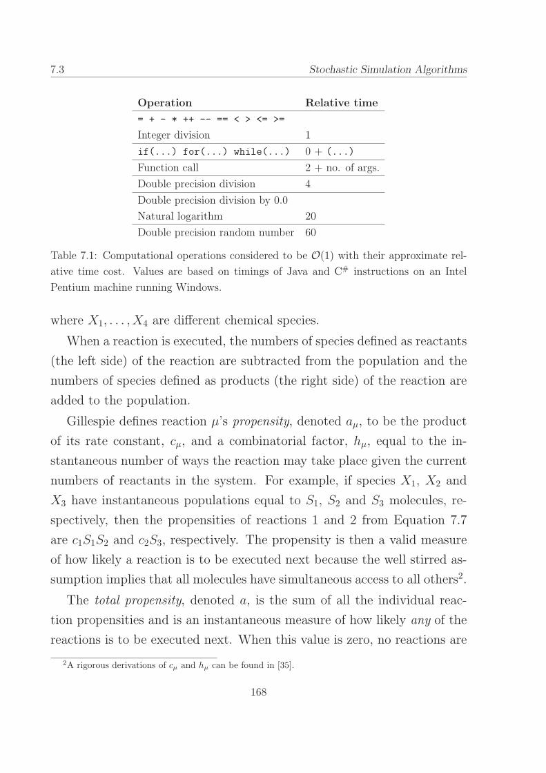
7.3 Stochastic Simulation Algorithms
Operation Relative time
= + - * ++ -- == < > <= >=
Integer division 1
if(...) for(...) while(...) 0 + (...)
Function call 2 + no. of args.
Double precision division 4
Double precision division by 0.0
Natural logarithm 20
Double precision random number 60
Table 7.1: Computational operations considered to be O(1) with their approximate rel-
ative time cost. Values are based on timings of Java and C# instructions on an Intel
Pentium machine running Windows.
where X1, . . . , X4 are different chemical species.
When a reaction is executed, the numbers of species defined as reactants
(the left side) of the reaction are subtracted from the population and the
numbers of species defined as products (the right side) of the reaction are
added to the population.
Gillespie defines reaction µ’s propensity, denoted aµ, to be the product
of its rate constant, cµ, and a combinatorial factor, hµ, equal to the in-
stantaneous number of ways the reaction may take place given the current
numbers of reactants in the system. For example, if species X1, X2 and
X3 have instantaneous populations equal to S1, S2 and S3 molecules, re-
spectively, then the propensities of reactions 1 and 2 from Equation 7.7
are c1S1S2 and c2S3, respectively. The propensity is then a valid measure
of how likely a reaction is to be executed next because the well stirred as-
sumption implies that all molecules have simultaneous access to all others2.
The total propensity, denoted a, is the sum of all the individual reac-
tion propensities and is an instantaneous measure of how likely any of the
reactions is to be executed next. When this value is zero, no reactions are
2A rigorous derivations of cµ and hµ can be found in [35].
168
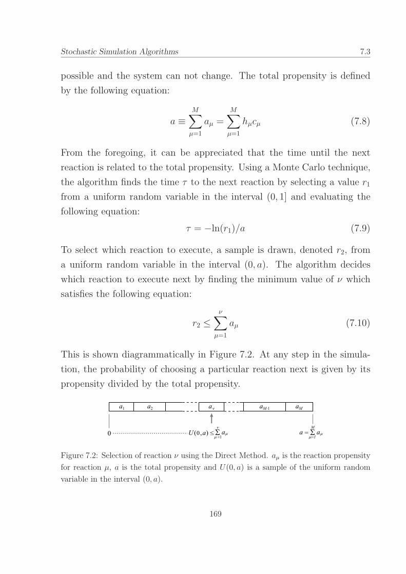
Stochastic Simulation Algorithms 7.3
possible and the system can not change. The total propensity is defined
by the following equation:
a ≡M
∑
µ=1
aµ =M
∑
µ=1
hµcµ (7.8)
From the foregoing, it can be appreciated that the time until the next
reaction is related to the total propensity. Using a Monte Carlo technique,
the algorithm finds the time τ to the next reaction by selecting a value r1
from a uniform random variable in the interval (0, 1] and evaluating the
following equation:
τ = −ln(r1)/a (7.9)
To select which reaction to execute, a sample is drawn, denoted r2, from
a uniform random variable in the interval (0, a). The algorithm decides
which reaction to execute next by finding the minimum value of ν which
satisfies the following equation:
r2 ≤ν
∑
µ=1
aµ (7.10)
This is shown diagrammatically in Figure 7.2. At any step in the simula-
tion, the probability of choosing a particular reaction next is given by its
propensity divided by the total propensity.
Figure 7.2: Selection of reaction ν using the Direct Method. aµ is the reaction propensity
for reaction µ, a is the total propensity and U(0, a) is a sample of the uniform random
variable in the interval (0, a).
169
7.3 Stochastic Simulation Algorithms
The First Reaction Method
At each step, the FRM calculates putative time increments for all possible
reactions in the system and executes the one with the shortest. The incre-
ment in simulated time for reaction µ is denoted τµ and calculated using a
similar Monte Carlo method to that used in Equation 7.9:
τµ = − ln(ran[0, 1))/(cµhµ) (7.11)
where ran[0, 1) is a number drawn from a uniform random variable in the
range [0, 1) and cµhµ is the propensity of reaction µ.
7.3.2 The Next Reaction Method
The Next Reaction Method (NRM) [31] builds on the FRM to achieve
a significant improvement in efficiency for typical biochemically reacting
systems. An improvement in complexity from O(M) to O(logM) of an
individual reaction step is gained, where M is the number of reactions in
the system. The key modifications are as follows:
• Reaction dependency graph: After the execution of each reaction,
Gillespie’s FRM re-calculates all the propensities in the system and
then re-generates the random putative times of the reactions. This
has complexity O(M). In biological systems, however, it is often the
case that reactions have limited dependency and only a fraction of
all the propensities change at any step. By initially constructing a
reaction dependency graph, during the simulation the algorithm need
only update those propensities which it knows could have changed.
Reaction dependency in typical biological pathways is typically much
less than M (e.g., see Figures 7.3 and 5.17) and hence the authors
of the NRM assume the reaction dependency graph to be ‘sparse’,
170

Stochastic Simulation Algorithms 7.3
i.e. dependency asymptotically unimportant.3 Under this assumption
the propensity update step drops out of the overall complexity of the
algorithm.
• Absolute time: The FRM and DM generate simulated time increments
which are relative to the current time of the simulation. By consider-
ing reaction times relative to t0, thus absolute time, the NRM is able
to re-use the putative times of reactions whose propensities have been
changed by the firing of the selected reaction. The formula
τµ,new = t+ (τµ,old − t)aµ,old/aµ,new (7.12)
where τµ and aµ are the absolute putative time and the propensity of
reaction µ, respectively, and t is the current simulated time, is thus
used to update the putative times of the dependent reactions.4 In this
way the NRM need only generate one random number per simulation
step - an additional saving over the DM.
• Indexed priority queue: The FRM requires O(M) operations to find
the reaction with the shortest time in an unordered linear data struc-
ture. By arranging the reaction times in a partially ordered binary tree
(called an indexed priority queue in [31]), such that the root holds the
reaction with the shortest time and reactions further from the root al-
ways have longer times than those closer (reactions at the same height
are not ordered), it is possible to select the fastest reaction in O(1)
operations. When the root reaction is executed, its propensity and
those of an arbitrarily located set of dependent reactions in the tree
changes. Since it is not necessary to maintain a horizontal ordering,
the authors provide an algorithm which applies pairwise exchanges
3It seems likely from empirical evidence that the dependency is something like O(log M) or O(M1/k),
where k > 1.4While aµ,new = 0, tµ,new is set to ∞. Immediately thereafter τµ is calculated afresh.
171
7.3 Stochastic Simulation Algorithms
of reactions at adjacent heights in the tree to maintain the tree’s in-
variant property. This has complexity proportional to the number
of reactions that change (the reaction dependency) multiplied by the
height of the tree. Since it has already been assumed that the average
reaction dependency of the system is sparse, the overall complexity of
selecting a reaction becomes O(logM).
Combining the effects of the itemised modifications gives an overall asymp-
totic complexity for the NRM of O(logM).
A particular drawback of the NRM is that even if there is a well defined
average order of reaction speeds that is constant throughout the course of
the simulation, the algorithm may still spend much time re-ordering the
tree. Following the execution of a reaction, the new times calculated for
the dependent reactions, being samples of random variables, alter their
positions in random ways. The significance of this effect depends on the
stochasticity of the reactions and how inherently well ordered the reactions
are.
7.3.3 Approximate methods
This section contains a brief overview of approximate simulation methods
which link the exact methods to the commonly used reaction rate equation
of chemical kinetics. In what follows Xi(t) is the number of molecules of
species i at time t and X(t) is the vector of such quantities at time t,
given that the system was at X(t0) = x0 at some initial time t0. x is
an instantaneous system state vector and aj(x) is the propensity of the
jth reaction, given that X(t) = x. This nomenclature is consistent with
a recent review of stochastic simulation [39], which may be consulted for
more detail.
172

Stochastic Simulation Algorithms 7.3
Species Dependent
µ Reaction affected reactions Dµ |Dµ|1. gA → MA + gA MA 6,12 2
2. pA + gA → g A pA,gA,g A 1,2,3,8,10,15,16 7
3. g A → MA + g A MA 6,12 2
4. gR → MR + gR MR 7,13 2
5. g R → MR + g R MR 7,13 2
6. MA → pA MA,pA 2,6,8,10,12,15 6
7. MR → pR MR,pR 7,8,11,13 4
8. pA + pR → AR pA,pR,AR 2,8,9,10,11,15 6
9. AR → pR AR,pR 8,9,11 3
10. pA → * pA 2,8,10,15 4
11. pR → * pR 8,11 2
12. MA → * MA 6,12 2
13. MR → * MR 7,13 2
14. g R → pA + gR g R,pA,gR 2,4,5,8,10,14,15 7
15. pA + gR → g R pA,gR,g R 2,4,5,8,10,14,15 7
16. g A → pA + gA g A,pA,gA 1,2,3,8,10,15,16 7
Mean |Dµ| = 4.06
Figure 7.3: Reaction dependencies of the noise-resistant oscillator model of Figure 5.11,
whose average dependency is 4.06. If S is the set of species and R is the set of reactions
r1 . . . rµ . . ., Dµ = r : R| |product j(rµ)| 6= |reactant j(rµ)| ∧ product j(rµ) ∪ reactant j(rµ) ∈reactants(r), 1 ≤ j ≤ |S|. That is, for a chosen reaction rµ, Dµ is the set of reactions
whose propensities are affected by its execution.
173

7.3 Stochastic Simulation Algorithms
Tau-leaping
The term ‘tau-leaping’, coined in [37], refers to the process in an approx-
imate stochastic simulation algorithm of simulating several individual re-
action events by a single aggregated event, thus leaping over several steps.
Under the condition that the aj(x) remain approximately constant during
the time interval [t, t+ τ ], the following equation (the tau-leaping formula)
is a good approximation of the evolution of the system:
X(t+ τ).= x +
M∑
j=1
Pj(aj(x)τ)νj (7.13)
where P(m) is the Poisson random variable with mean m and τ is the
length of the leap. When the conditions of applicability are met, a tau-
leaping simulation algorithm thus generates samples of the appropriate
Poisson random variable and uses the value to make multiple simultaneous
applications of the corresponding reaction.
Selecting values of τ which maximise leap size to gain efficiency, yet
avoid inaccuracy, instability and negative populations, is non-trivial and
the subject of ongoing research [41, 12, 9]. Stiff systems, which have both
fast and slow time-scales and where the fastest modes are stable, require τ
to be small on the fastest time-scale to retain accuracy. Since stiff systems
are common, several strategies have been devised, such as the implicit tau-
leaping method [75] and the Slow Scale Stochastic Simulation Algorithm
(ssSSA) [11]. See Section 7.3.3.
The Chemical Langevin Equation
Knowing that N (m,σ2) = m + σN (0, 1), where N (m,σ2) is the normal
random variable with mean m and variance σ2, and that P(m) ≈ N (m,m)
174

Stochastic Simulation Algorithms 7.3
for m≫ 1, Equation 7.13 can be re-written
X(t+ τ).= x +
M∑
j=1
νjaj(x)τ +M
∑
j=1
νj
√
aj(x)τ Nj(0, 1)√τ (7.14)
Equation 7.14 is then a good approximation to the evolution of the sys-
tem when both aj(x) remain sufficiently constant and the copy number
of molecules is much greater than 1. Equation 7.14 can be written in
continuous form
dX(t)
dt.=
M∑
j=1
νjaj(X(t)) +M
∑
j=1
νj
√
aj(X(t)) Γj(t) (7.15)
where Γj(t) are statistically independent white noise processes. Equation
7.14 is the standard form Chemical Langevin Equation (CLE) while Equa-
tion 7.15, an alternative form of the CLE, has the canonical form of a
stochastic differential equation, containing a deterministic drift term and
a stochastic diffusion term.
The Reaction Rate Equation
In the thermodynamic limit, that is, the case when the system volume Ω and
species populations X tend to infinity such that their concentrations X/Ω
remain constant, the system is well approximated by Equation 7.15. Under
these conditions the propensity functions aj(x) grow in proportion to the
size of the system (i.e., the magnitudes of the species populations) and the
drift and diffusion terms of the CLE are thus affected unequally. The drift
term increases in proportion to the system size while the diffusion term
grows as the square root of the system, hence as the system approaches
the thermodynamic limit, the stochastic term disappears and what remains
is the familiar deterministic reaction rate equation (RRE):
dX(t)
dt=
M∑
j=1
νjaj(X(t)) (7.16)
175
7.3 Stochastic Simulation Algorithms
Quasi Steady State Stochastic Simulation Algorithms
Inspired by the well-known Michaelis-Menten approximation for enzyme
kinetics, several approaches to stochastically simulating stiff chemical sys-
tems are based on a quasi steady-state approximation [74]. See also, e.g.,
[44], [10] and [11]. The following subsection describes the slow scale Stochas-
tic Simulation Algorithm (ssSSA) [11] to exemplify these approaches.
The slow scale Stochastic Simulation Algorithm
The ssSSA first makes a partition of the reactions into fast and slow sets.
The fast set contains those reactions whose propensity functions tend to
have the largest values and the slow set contains the rest. The species
are also partitioned into into fast and slow subsets. Any species which
is affected by a fast reaction is classified as a fast species, the rest are
classified as slow. It is then possible to partition the overall process into
fast and slow processes Xf(t) and Xs(t), respectively, where Xs(t) involves
only slow species and slow reactions but Xf(t) involves fast reactions and
both fast and slow species.
The virtual fast process Xf(t) is defined as the fast species evolving as
a result of the fast reactions with the slow reactions turned off.
For the ssSSA to be applicable, the system must satisfy two stochastic
stiffness conditions: Xf(t) must approach a well defined time-independent
random variable Xf(∞) as t→∞ and Xf(t)→ Xf(∞) must be achieved
in a time which is small compared with the time to the next slow reaction.
The slow scale approximation [11] then asserts that it is acceptable to
ignore the fast reactions and simulate the system one slow reaction at a
time, provided that the propensity function of each slow reaction is replaced
by its average with respect to the asymptotic virtual fast process Xf(∞).
The ssSSA thus simulates the slow reactions using the average propen-
176

Stochastic Simulation Algorithms 7.3
sity functions and ignores the fast reactions. The fast species can be ob-
tained by Monte Carlo sampling.
Note that the multiscale stochastic simulation algorithm [10] differs from
the ssSSA in the way the averages are computed and the way in which the
fast species populations are generated, but is otherwise similar.
7.3.4 Numerical precision
It is important to note here that the random numbers used in stochas-
tic simulations as described above should have sufficient precision to ade-
quately represent the granularity of the range of propensities and times that
occur during a simulation. A simple illustration of how a problem might
arise for an algorithm based on the Direct Method is the case of simulated
system having three reaction channels but the random number used to se-
lect them having only one bit of precision: a single sample would not be
able to distinguish the reactions. A more likely problem is that the ratios
of instantaneous propensities or times can not be accurately represented
by the random number. For example, suppose a simulation algorithm has
a uniform random number generator with eight bits of precision (so 256
different equally likely values) and a model to be simulated contains two
reactions which have respective propensities of 1 and 400 at some point
during the simulation: the reactions can not be accurately selected by the
algorithm because the random number generator does not have sufficient
precision to represent the ratio 1:400. In general, floating point numbers
are represented in a computer with a fixed window of precision plus an
exponent which allows the window to slide over a much wider range of
values. The problems of precision may therefore be more subtle.
For algorithms based on the first reaction method an analogous situation
is that two or more reactions have exactly the same time of execution or
that a reaction ends up having zero or infinite time. For the case of the next
177

7.3 Stochastic Simulation Algorithms
reaction method, which uses absolute time, there is an additional burden
of numerical precision. Reaction events continue to occur separated by
the same time-scales found in the other exact algorithms (since they all
produce equivalent traces), yet the values of time used and stored by the
NRM are of the order of the total length of the simulation. To distinguish
new reaction events, the numbers are thus required to maintain precision
at extreme orders of magnitude, with the eventual result that lower order
bits get lost.
Concerning the Direct Method, if the lowest significant figure of the
largest propensity represents a greater value than the highest significant
figure of another propensity, then the reaction corresponding to the smaller
propensity can not be selected. Moreover, algorithms which update the
total propensity using the change in propensity at each step, rather than
performing a complete summation, run the risk of additional error due to
a related limitation. The conditions that cause the error to arise are that
during a simulation there are a number of reactions which have individual
propensities whose lowest significant figure has a lower value than the value
of the lowest possible significant figure of the total propensity at its current
value. It is then conceivable that the change in propensity caused by the
application of two or more such reactions is different to the change that
would be caused by applying the sum of their changes.
The consequences are that the stored total propensity is different to
the real total propensity and that the error may grow, dependent on the
nature of the model, the simulation conditions and other factors such as
the machine’s precision and rounding policy. For the case that the stored
total propensity is less than the real total propensity, the effect will be most
strongly felt by the reactions that occur at the end of the summation: they
will not be fully covered by the random sample r2 and will be selected less
frequently. In the worst case this could be not at all: if the reactions are
178

Stochastic Simulation Algorithms 7.3
ordered to increase the performance of selection, then those with the lowest
propensities will lie at the end of the summation and their propensities
might be less than the accumulated error. Reactions with low propensities
might also fall at the end of the summation by chance, so this problem is
not limited to algorithms which order the reactions in such a way.
179

7.3 Stochastic Simulation Algorithms
180

Chapter 8
The Method of Partial Propensities
Agent based paradigms are emerging as a promising computational for-
malism to represent the complexity of biological systems and one such,
Colonies of Synchronising Agents, has been presented in Chapter 6. It
turns out, however, that to simulate the CSA model involves a high level
of computational complexity. This is in part due to the fact that agents, not
being atomic, must be represented individually and simulated discretely.
The Gillespie algorithm [32] and its derivatives are widely used in Com-
putational Biology as relatively efficient means to simulate the discrete
interaction of chemical species. This efficiency relies on a description of
chemistry which treats populations of molecules as a ‘well stirred’ mix-
ture of identical hard spheres. This, in effect, removes the concepts of
space and molecular individuality from the formulation and exploits the
resulting symmetries. By contrast, agent based paradigms such as CSA re-
introduce individuality and thus lose the advantageous symmetries. The
computational complexity rises in a combinatorial way.
In developing a software realisation of the CSA model, a stochastic
simulation algorithm has been devised which significantly ameliorates the
computational complexity in comparison to standard approaches. It is ob-
served that while some of the symmetries of a well stirred system have been
181
8.1 The Method of Partial Propensities
removed, others have been introduced and it is these that are exploited.
Though the present motivation is to model complex biological systems as
they might be in-vivo, the algorithm can also be applied to efficiently simu-
late experiments where there is structured repetition of chemical reactions.
Moreover, the technique may be beneficial in other stochastic agent-based
or hierarchical systems where there is combinatorial interaction.
8.1 Introduction
There is growing interest in Computational Systems Biology to perform
discrete and stochastic simulations of chemically reacting systems; the in-
tuition being that this technique provides additional insight about what
are essentially stochastic biological processes. More precisely, the ratio-
nale is that stochastic simulation using discrete quantities of molecules,
rather than continuous concentrations, can reveal behaviour that is hidden
by the averaging effect of deterministic simulation of ordinary differential
equations. In addition, the discrete approach lends itself to analysis by
the tools of computing science formal methods, such as model checking.
The penalty of this technique is the computational complexity of simulat-
ing every individual interaction between populations, although the current
algorithms and hardware keep the task more or less tractable, if not trivial.
As systems biologists’ ambitions grow, however, and bigger systems with
more complex phenomena are modelled, there will be an inevitable increase
in the computational complexity associated with simulation. In particu-
lar, agent-based modelling frameworks offer the possibility to model the
complex interaction of populations of objects which may themselves have
complex internal behaviour. By using such a formalism it is possible to
reduce the complexity of the description of a complex system by hierar-
chical composition: define behaviour at a microscopic level, call that an
182
The Method of Partial Propensities 8.1
agent and then define the interaction of populations of agents at a macro-
scopic level. Each member of the population is then potentially a unique
individual with a unique internal state which must be tracked. While the
description may be simple, the complexity of the system manifests itself as
a combinatorial explosion of states in the unfolding simulation.
In this context, the hierarchical computational paradigm and modelling
framework Colonies of Synchronizing Agents (CSA) has been presented in
Chapter 6. The key points to note about CSA for the present context are
that agents may contain arbitrary, independent chemically reacting sys-
tems and may interact with each other in a chemistry-like way according
to their type (a dynamic property), optionally controlled by their internal
chemistry (internal reactions). A set of synchronisation reactions (agent re-
actions) is specified to define how agents react with one another and these
depend on the internal state of the agents. While the representation of
the agents is necessarily discrete, the representation of their internal chem-
istry is also represented in a discrete way in the CSA model to facilitate
homogeneous simulation and logical analysis (see Chapter 6).
The quantities of agents and chemical species are therefore discrete and
the evolution of the system is stochastic. Contrary to intuition perhaps, us-
ing a discrete approach to represent agents is potentially more efficient than
simulating the same system with ordinary differential equations (ODEs).
The reason behind this is that ODEs are efficient to represent large popu-
lations of small numbers of species, since small and large populations have
equivalent complexity when represented by a single real number, but each
species represents a differential equation to be solved. In the CSA model,
each agent corresponds to a unique species in a population of magnitude
one, which would therefore be computationally cumbersome in an ODE
framework.
Currently, the most popular and efficient approach to discrete and stochas-
183
8.2 The Method of Partial Propensities
tic simulation is the implementation of some derivative of the Gillespie
algorithm [32] (e.g. [13, 11, 31, 37]), which was designed to simulate tra-
jectories of chemically reacting systems which are exactly consistent with
the chemical master equation. In what follows, a basic understanding of
the Gillespie algorithm is assumed and may be gained from Section 7.3.1.
More detailed treatment can be found in the original papers [32, 33, 35],
the reviews [39, 40] and the book [34]. Section 8.2 first recaps some ba-
sic terminology then considers the computational complexity of the direct
method (DM) and the additional complexity entailed in its application to
the CSA model. Techniques are then described which significantly reduce
this complexity and it is shown show how these improve on benchmark
algorithms. In doing this, it is also shown how the techniques have gen-
eral applicability in contexts where there is combinatorial-like interaction
between populations of objects.
In what follows the reader is assumed to be familiar with the basic con-
cepts and terminology of exact stochastic simulation methods as outlined
in Section 7.3.1.
8.2 The Direct Method
The Gillespie algorithm is an efficient way to exactly simulate a trajectory
of a chemically reacting system, which are often intractable to analysis and
more easily investigated by simulation [33]. Exact in this context means
that the trajectories so generated are fully consistent with the premises
that underlie the chemical master equation (CME). In what follows, the
focus is on the direct method (DM) since it is most readily adapted for
the current purpose and most easily understood. It is noted here, however,
that the techniques described in Section 8.3 are not limited to the DM.
184

The Method of Partial Propensities 8.2
8.2.1 Computational complexity of the DM
The average number of steps of an exact discrete and stochastic simulation
of a chemically reacting system is critically dependent on the nature of
the model, the initial numbers of molecules and the length of time being
simulated, but it is independent of the algorithm used because, by definition
of the term exact, the simulations are samples of the sme distribution.
Since the number of steps cannot therefore be reduced without skipping
reaction events and thus losing exactness, improving the efficiency of an
exact stochastic simulation algorithm requires the reduction of the cost of
an individual iterative step.
The asymptotic computational complexity of the DM is now considered
in terms of input being the number of reactions, M , using the terminology
defined in Section 7.3.1.
The direct method can be summarised thus:
1. initialise species and set time = 0.
2. iterate for sufficient steps or until all propensities are zero:
a calculate M propensities
b sum M propensities to give a, the total propensity
c generate random number r1
d calculate τ using Equation 7.9 and add to time
e generate random number r2
f sum reaction propensities in order until value just greater than r2
g update species according to the reaction reached in step 2.f
Steps 2.a and 2.b each require a number of operations proportional to
M and hence are O(M). Steps 2.c, 2.d and 2.e involve calls to costly
185
8.2 The Method of Partial Propensities
mathematical functions which generate random numbers and logarithms,
however the cost does not increase with input size and is therefore O(1)
(see Table 7.1). Step 2.f will usually take fewer than M operations, but
scales as O(M). The number of species affected by a reaction is often a
small number only weakly related to M , so step 2.g is often assumed to be
O(1). Summing these, the overall asymptotic complexity is O(M)
8.2.2 Optimizations of the DM
The following optimisations are features of the Optimized Direct Method
(ODM) of [13], not to be confused with the algorithm of the same name
featured in the appendix of [31].
The DM relies on a selection made from the cumulative sum of propensi-
ties, where each value in the accumulation is dependent on all summations
up to that point. If one propensity changes, then all the cumulative propen-
sities that follow it must be re-calculated. In general, the application of
a reaction affects the propensities of the other reactions unpredictably, al-
though it is unlikely to affect all the other reactions. Hence, it is not always
necessary to recalculate all the propensities, but it does seem necessary to
re-calculate all the cumulative propensities. The following optimizations
address these issues:
1. By creating a reaction dependency graph [31] it is necessary to update
only the propensities of those reactions which have changed. Step 2.a
then reduces to O(1), under the assumption that reaction dependency
is only weakly related to M .
2. By storing the intermediate sums of step 2.b in an array it is possible to
reduce step 2.f to an O(logM) search. Since the values are monotonic,
the desired reaction can be found by iteratively dividing the array
186

The Method of Partial Propensities 8.3
according to whether the desired value is above or below a mid point.
However, this optimization is superseded by the following:
3. By storing the total propensity, a, and updating it at each step by
the sum of the differences of changed propensities, it is possible to
avoid summing M propensities in either step 2.b or step 2.f. It is only
necessary to sum until the value defined by r2 is reached, which is ≤M
operations. If it is possible to arrange the reactions in descending order
of frequency, the worst case average summation will beM/2 operations
(when all the reactions are equally likely), with a best case being
significantly better (see Figures 9.1 and 9.2). Like Optimization 1.,
this optimization relies on the assumption that reaction dependency
is O(1).
4. Thus, by initially calculating and storing all the propensities, it is
possible to avoid re-calculating unchanged propensities during the it-
eration.
8.3 The Method of Partial Propensities
The Method of Partial Propensities (MPP) has been specifically designed
to ameliorate the computational complexity of simulation the CSA model.
The terminology given in Section 7.3.1 and used above is thus extended to
accommodate the various extended concepts it contains.
A colony consists of N agents, each containing a maximum of S differ-
ent chemical species, MI internal reactions and MA agent reactions, where
M ≡MI +MA. The reactions are global, i.e., they apply to all agents, how-
ever reactions may be disabled with respect to certain agents by altering
the agents’ contents. Internal reactions can be considered chemistry of the
type described in Section 8.2, however agent reactions are an abstraction
187

8.3 The Method of Partial Propensities
of this concept and need further explanation.
An agent reaction is applicable to a pair of agents and contains two
sets (strictly multisets, see Chapter 2) of reactants which must exist in
their corresponding agents for the reaction to be executed. In contrast to
internal reactions and the chemical reactions defined in [32], which have a
maximum of three reactants, there is no theoretical limit to the number of
elements of either of these two sets. An agent reaction also contains two
sets of products which correspond with the sets of reactants. When an
agent reaction is executed, the species in the sets of reactants are removed
from their corresponding agents and species defined in the corresponding
sets of products are added accordingly. An agent reaction therefore has
the general form
V1, . . . , Vk+ W1, . . . ,Wlcµ→ X1, . . . , Xm+ Y1, . . . , Yn (8.1)
where cµ is the constant reaction rate, V1, . . . , Vk and W1, . . . ,Wl are
sets of necessary reactants in the first and second agents, respectively,
X1, . . . , Xm and Y1, . . . , Yn are the respective sets of products, and
k . . . n are arbitrary integers.
The state of the colony is evolved by applying a sequence of reactions
which are chosen randomly according to their average rate and an expo-
nential distribution. In order to maintain this Markovian property, so that
the system may be simulated in the manner of the Gillespie algorithm, the
propensities of agent reactions, like those of internal reactions, are func-
tions of the current state of the system only. The propensity of an internal
reaction is calculated with respect to the populations of species contained
within a specific agent. The propensity of an agent reaction refers to a
specific pair of agents and is calculated as the number of ways that the
reaction’s first set of reactants may be selected from the first agent, mul-
tiplied by the number of ways its second set of reactants may be selected
188
The Method of Partial Propensities 8.3
from the second agent, multiplied by a rate constant.
8.3.1 Computational complexity of CSAs using the DM
In this section the cost of simulating the CSA model is considered with
respect to the DM, in order to gain an understanding of the increased
complexity. The following description therefore takes the same form as
that of Section 8.2.1, however in this case the number of agents is also
considered as part of the input when evaluating the complexity. This is
because the number of reactions alone does not determine the total number
of propensities used by the algorithm.
aµi denotes the propensity of internal reaction µ in agent i. aπij denotes
the propensity of agent reaction π applied to agents i and j. In general,
aπij 6= aπji, hence propensities for all ordered pairs of agents are calculated
except the case when i = j, which is defined to be impossible and therefore
aπii ≡ 0.
The total propensity for internal reactions, aI , is defined by:
aI ≡N
∑
i=1
MI∑
µ=1
aµi (8.2)
The total propensity of agent reactions, aA, is defined by:
aA ≡N
∑
i=1
N∑
j=1
j 6=i
MA∑
π=1
aπij (8.3)
Hence, the total propensity of all the possible reactions at a given instant
is defined to be:
a ≡ aI + aA (8.4)
The total number of propensities is thus:
(N 2 −N)MA +NMI (8.5)
189

8.3 The Method of Partial Propensities
The time until execution of the next reaction, τ , will be calculated, as in
the case of the standard DM, by sampling the uniform random variable in
the range (0, 1] and evaluating Equation 7.9 using a defined in Equation
8.4.
A reaction is selected, as before, by first drawing a sample, r2, from
the uniform random variable in the interval (0, a). In general, propensities
are summed in order and the reaction to execute is that reached when the
value of the summation is just greater than or equal to r2.
Hence, by arranging the propensities such that propensities 1 . . .MI
correspond to the set of internal reactions and propensities (MI + 1) . . .M
correspond to the set of agent reactions, it is possible to say that for r2 ≤ aI
the reaction will be an internal reaction and an agent reaction otherwise.
For the case that r2 ≤ aI , the DM will choose internal reaction ν in agent
α, where α and ν satisfy
r2 ≤α
∑
i=1
ν∑
µ=1
aµi (8.6)
such that α is minimum and ν is minimum given α. For the case that
r2 > aI , the reaction will be agent reaction δ between agents β and γ,
where β, γ and δ satisfy
r2 ≤ aI +
β∑
i=1
γ∑
j=1
j 6=i
δ∑
π=1
aπij (8.7)
such that β is minimum, γ is minimum given β and δ is minimum given
β and γ. Note that, in general, to find α and ν or β, γ and δ to satisfy
Equations 8.6 and 8.7 requires the summation of O(NMI) or O(N 2MA)
propensities, respectively.
The DM applied to CSA can thus be summarised as:
1. initialise agents and internal species and set time = 0.
190
The Method of Partial Propensities 8.3
2. iterate for sufficient steps or until all propensities are zero:
a calculate all NMI +N 2MA propensities
b sum all NMI and N 2MA propensities to give aI , aA and thus a
c generate random number r1 using a
d calculate τ using Equation 7.9 and add to time
e generate random number r2 using a
f if r2 ≤ aI :
(i) sum propensities of internal reactions in order until just greater
than r2
g else if r2 > aI :
(i) sum propensities of agent reactions in order until just greater
than r2 − aI
h execute the reaction reached in the previous step
Steps 2.c, 2.d, 2.e and 2.h are O(1), as with the DM. Step 2.(f)(i) has
complexity O(NMI) and Step 2.(g)(i) has complexity O(N 2MA). Steps
2.a and 2.b have complexity O(NMI) + O(N 2MA). Hence the overall
complexity is O(NMI) +O(N 2MA).
While it might be expected that the internal chemistry ofN independent
agents will require N times as much computation as a single system, the
N 2 term may be seen as something of a surprise. The fact that each agent
potentially constitutes a unique agent specie means that agent reactions
effectively define a class of reactions containing all the possible pairs of
agents. In systems whereN ,MI andMA are all large, this result constitutes
a significant increase in complexity.
191

8.3 The Method of Partial Propensities
8.3.2 Details of the Method of Partial Propensities
The method of partial propensities (MPP) partitions the selection of one
reaction from a choice of (N 2−N)MA+NMI alternatives to a combination
of three or four simpler choices. These choices correspond to (i) whether
the reaction is internal or external; (ii) which agent is affected; (iii) which
other agent is affected (if an agent reaction); (iv) which agent reaction is
to be applied (if this is so) or (v) which internal reaction is to be applied.
The total propensity is constructed from summations which can be divided
into partial propensities which correspond to these choices. The individual
propensities form the contents of a two dimensional matrix and a three
dimensional matrix, corresponding to aI and aA, respectively. The partial
propensities are sums of elements in the rows and columns of these matrices
and are characterised as follows.
The choice of whether a reaction is internal or an agent reaction can be
made from partial propensities aI and aA, as described in Section 8.3.1.
Once this choice has been made, the choice of the first agent of an agent
reaction (or the only agent if an internal reaction has been chosen) is made
using N partial propensities A1, . . . , AN , where
Ai ≡N
∑
j=1
j 6=i
MA∑
π=1
aπij +
MI∑
µ=1
aµi (8.8)
The first agent, α, is chosen to be the minimum value which satisfies:
r2 ≤α
∑
i=1
Ai (8.9)
If the reaction is an agent reaction, the choice of the second agent is made
using N partial propensities B, . . . , BN , where
Bj ≡N
∑
i=1i6=j
MA∑
π=1
aπij (8.10)
192
The Method of Partial Propensities 8.3
The second agent, β, is chosen to be the minimum value which satisfies:
r2 ≤β
∑
i=1
Bi (8.11)
The choice of the agent reaction is made using MA partial propensities
C1, . . . , CMA, where
Cπ ≡N
∑
i=1
N∑
j=1
j 6=i
aπij (8.12)
Agent reaction γ is chosen to be the minimum value which satisfies:
r2 ≤γ
∑
i=1
Ci (8.13)
If the reaction was chosen to be internal, the choice of which one is made
using MI partial propensities D1, . . . , DMI, where
Dµ ≡N
∑
i=1
aµi (8.14)
Internal reaction ν is chosen to be the minimum value which satisfies:
r2 ≤ν
∑
i=1
Di (8.15)
There are therefore 3N + MI + MA partial propensities generated by
Equations 8.8, 8.10, 8.12 and 8.14, plus aI and a, which must all be updated
after the execution of a reaction. This value is O(N) times fewer than the
total number of propensities.
The execution of an internal reaction affects a maximum of MI other
propensities (i.e., only those relating to reactions in the same agent), while
the execution of an agent reaction affects the propensities of a maximum
of 2(MAN − 1 + MI) agent reactions (i.e., the reactions of all the other
agents in the colony reacting with the two involved in the current reaction,
193

8.3 The Method of Partial Propensities
plus the internal reactions of the two changed agents.). If the set of in-
ternal reactions is based on biochemical pathways, the number of internal
reactions affected by the execution of an internal reaction is likely to be
much less than MI , even when an agent contains multiple pathways (see
Figures 5.17 and 7.3), however the cost of updating propensities, which is
O(NMA) + O(MI), still contains an O(MI) term as a result of the effect
of the agent reactions. This is nevertheless O(N) times less than the total
number of propensities given in Equation 8.5.
Hence, the MPP makes an initial calculation of all the propensities
and partial propensities, but thereafter updates only the propensities and
partial propensities that change. By then selecting the next reaction to
execute using the partial propensities, the overall gain in efficiency relative
to the direct method applied to the CSA model is therefore O(N).
The method of partial propensities can be summarised as follows:
1. initialise agents and internal species and set time = 0.
2. ascertain and store internal reaction dependency and internal reaction
dependency on agent reactions
3. calculate and store all (N 2 −N)MA +MI propensities
4. sum propensities to generate and store 3N +MI +MA partial propen-
sities plus aI and a
5. iterate for sufficient steps or until all propensities are zero:
a generate random number r1 using a
b calculate τ using Equation 7.9 and add to time
c generate random number r2 using a
d sum partial propensities Ai to find α, the minimum value to satisfy
Equation 8.9
194

The Method of Partial Propensities 8.4
e if r2 ≤ aI :
(i) sum partial propensities Di to find ν that is the minimum
value that satisfies Equation 8.15
(ii) execute reaction ν in agent α
(iii) re-calculate propensities of internal reactions of agent α ac-
cording to internal reaction dependency.
(iv) re-calculate the MA(N−1) agent reaction propensities involv-
ing agent α
f else if r2 > aI :
(i) sum partial propensities Bi to find β, the minimum value to
satisfy Equation 8.11
(ii) sum partial propensities Ci to find γ, the minimum value to
satisfy Equation 8.13
(iii) execute agent reaction γ between agents α and β
(iv) re-calculate internal reaction propensities for agents α and β
according to internal reaction dependency on agent reaction
γ.
(v) re-calculate the 2MA(N − 1) agent reaction propensities in-
volving agents α and β
8.4 Results
While the theoretical basis for the MPP is clear, it is felt necessary to have
a practical demonstration of its increased efficiency relative to benchmark
algorithms. In particular, it is desirable to see evidence of the algorithms’
comparative scaling with increased model size. This is a somewhat artifi-
cial requirement in terms of biological modelling, hence it is necessary to
195
8.4 The Method of Partial Propensities
construct a set of biologically plausible artificial models which present an
increasing load.
The unit of load is chosen to be the noise-resistant oscillator (NRO) of
Figure 5.11, which although not a real biological model is nevertheless bio-
logically inspired. Moreover, it has the characteristic of being ‘multi-scale’
in a plausibly biological way (see Figure 9.2) and has a suitable number of
reactions. The more biological model of NF-κB oscillation (Figure 5.16)
was also considered, however its larger size makes it unsuitable as the unit
of model generation: the problem almost immediately becomes intractable
to all algorithms and no clear trend is established.
In order to allow the widest possible valid comparison of algorithms and
models, the NRO is used in a way that simulates the increased computa-
tional load of a CSA model using standard chemical reactions. Precisely,
the NRO reactions are considered to be a set of 16 agent reactions which
have an average dependency of approximately four (see Figure 7.3). For
the simplest case, a benchmark model is created which contains two sets of
identical NRO reactions. This then has double the dependency of the sin-
gle model, since each reaction has one set of dependent reactions from the
first instance and an identical set from the second. Such a model replicates
the situation of a colony with two agents.
By thus creating models with increasing numbers of copies of the NRO
model it is possible to simulate the algorithmic load presented by colonies
with increasing numbers of agents: the dependency grows proportional to
the number of copies but the number of different types of reaction does
not grow.1
By adopting this strategy it is then possible to create a set of benchmark
models which may be simulated on a variety of platforms for comparison.
1Note that by using a single set of species and dividing the original reaction rates by the number of
‘agents’, the observed behaviour of the species populations will be identical to a single instance of the
model.
196

The Method of Partial Propensities 8.4
The results of a preliminary investigation are shown in Figure 8.1, where
the ‘impossible’ case of one agent is included for reference (this made possi-
ble by virtue of the way the benchmarks are generated). In order to include
the MPP it was necessary to create a version of the algorithm which takes
standard chemical systems as input but can take advantage of the struc-
ture of the models. Algorithmic scaling of systems containing up to ten
agents seems to conform to theory: the DM scales as O(N 2), the MPP
scales as O(N) and the NRM scales as O(N logN). The ODM initially
scales at a similar rate to the MPP and NRM but eventually reverts to
O(N 2). This is because the ODM is initially able to take advantage of the
inherently logarithmic distribution of reactions but combining parallel in-
stances of logarithmically distributed systems, as here, does not maintain
a logarithmic distribution. See Figure 9.4.
In addition to the asymptotic scaling, the constant ratios between the
algorithms are also evident in Figure 8.1. The relatively light implementa-
tional weight of the MPP and ODM make them approximately three times
faster than the NRM at the left hand side of the graph. The DM, included
for reference, is slow due to not having the benefit of the optimisations of
the ODM and MPP. The small additional implementational complexity of
the MPP relative to the ODM also seems evident on the left hand side of
the figure: the MPP’s technique does not have an advantage for the case
of one agent. Perhaps surprisingly, above ten agents the effects of low level
memory caching (i.e., not disk caching and therefore not under the control
of the operating system) affect the measured performance and the theo-
retical trends are lost. Instruction counting confirms that the theoretical
trends continue, however it is not possible to overcome the limitations of
the hardware. The memory effects eventually dominate the performance
and since the memory usage of all the algorithms is O(N 2), this is the
asymptotic scaling. Importantly, however, although the algorithms scale
197
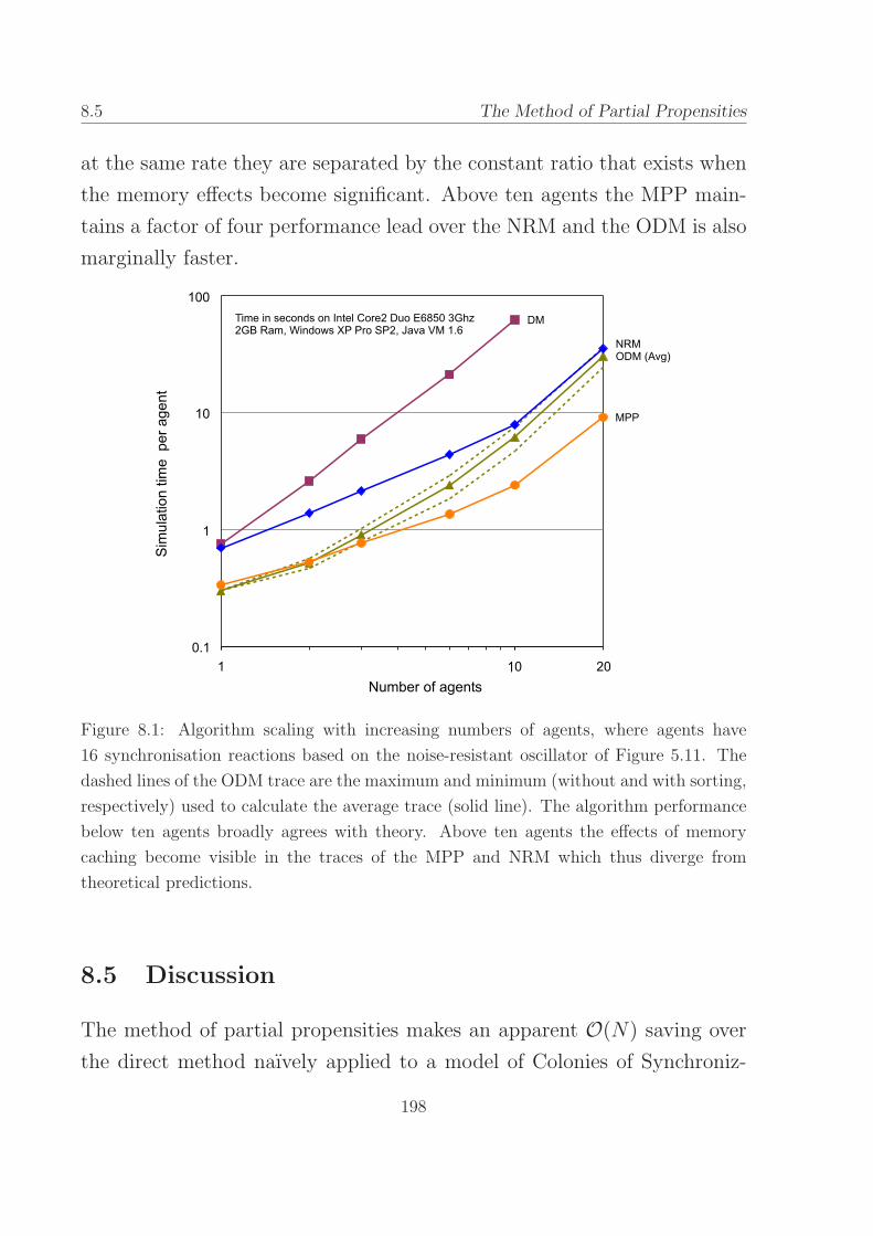
8.5 The Method of Partial Propensities
at the same rate they are separated by the constant ratio that exists when
the memory effects become significant. Above ten agents the MPP main-
tains a factor of four performance lead over the NRM and the ODM is also
marginally faster.
Figure 8.1: Algorithm scaling with increasing numbers of agents, where agents have
16 synchronisation reactions based on the noise-resistant oscillator of Figure 5.11. The
dashed lines of the ODM trace are the maximum and minimum (without and with sorting,
respectively) used to calculate the average trace (solid line). The algorithm performance
below ten agents broadly agrees with theory. Above ten agents the effects of memory
caching become visible in the traces of the MPP and NRM which thus diverge from
theoretical predictions.
8.5 Discussion
The method of partial propensities makes an apparent O(N) saving over
the direct method naıvely applied to a model of Colonies of Synchroniz-
198

The Method of Partial Propensities 8.5
ing Agents with N agents. While this is significant, it might have been
conjectured that the Next Reaction Method (NRM) [31], which apparently
offers O(log(number of propensities)) complexity, will be trivially more effi-
cient. The fallacy of this is that the NRM has complexity more accurately
described as O(d log(number of propensities)), where d is the average de-
pendency of reactions. In biochemical systems d is usually only weakly
related to M , perhaps O(logM) or O(M 1/k) for some k > 1). In contrast,
the dependency of CSA agent reactions is O(NMA), so the NRM applied
to these has complexity O(NMA log(NMA)), compared to O(NMA) of the
MPP. It seems that for agent reactions, at least, the method of partial
propensities will outperform the benchmark NRM.
It has been observed by others [10, 13] that biochemical systems of-
ten have a ‘multiscale’ distribution and this is corroborated by the exam-
ples in this chapter (see Figures 9.2 and 9.1). If agent reactions (mod-
elling, e.g., cell to cell communication) also have this distribution, then the
method of partial propensities will likely be the optimal choice even when
log2N < MA. Moreover, the MPP can take advantage of such multi-scale
distributions by judicious ordering of the reactions. Note, however, that
this has a lesser effect than in the ODM, for example, because the MPP is
already optimised not to need such ordering.
It might be supposed that internal reactions, corresponding to intracel-
lular pathways, do not have the same kind of combinatorial complexity of
agent reactions and therefore can not benefit from the techniques of the
MPP. Chapter 9 presents an algorithm which draws inspiration from the
MPP (the method of arbitrary partial propensities - MAPP) which is able
to consistently outperform the NRM when applied to test case models con-
structed in a similar way to the benchmark models described in Section
8.4. For the sake of presenting the main result relating to agent reactions,
the selection of an internal reaction has so far been assumed to be via an
199
8.6 The Method of Partial Propensities
optimised version of the direct method. The internal reactions may consti-
tute significant complexity in themselves however, so it is conceivable that
once the MPP has decided that the next reaction to execute is internal,
its selection will be achieved using a more efficient algorithm such as the
MAPP.
The method of partial propensities can also be applied to simulations
where there is a significant amount of either deliberate or accidental com-
binatorial or repetitious reactions. For example, the technique has been
previously used in a stochastic model of aggregation [57] and has appli-
cation in modelling microarray experiments. The general conditions of
applicability are that the system is large and consists of reactions which
form a well defined n-dimensional non-sparse array of propensities. The
requirement of being large is so that the gains can compensate the addi-
tional overhead. The requirement of the array not being sparse is so that
the number of propensities is large with respect to the number of partial
propensities such that a potential gain exists. In general, the number of
reactions in a given order (i.e., a class of reactions having the same number
of species used to calculate the propensity) must approximate Sn, where S
is the number of species and n is the order of the reaction. It is observed
here that under certain circumstances it might be advantageous to add a
‘dummy species’ to the set of species so that reactions of a lower order can
be included in a higher order for greater overall efficiency. For example,
X1 → X2 might be re-written as X0 + X1 → X2, where X0 would have a
constant value of 1.
8.6 Conclusion
One of the goals of systems biology is to model and simulate large systems
comprising smaller systems. When the smaller systems are themselves
200
The Method of Partial Propensities 8.6
complex there is a potential of high combinatorial complexity. In solving
such a problem specific to the implementation of Colonies of Synchronizing
Agents, a simple method has been devised that has utility and wider appli-
cation: the method of partial propensities. By partitioning the simulation
algorithm along the lines which generate the complexity, it is possible to
significantly ameliorate it. The methods presented in this chapter may
also be relevant to other hierarchical stochastic formalisms, such as those
based on process algebra or state charts, where complexity derives from
combinatorial effects.
In prospect is the incorporation into the MPP of an efficient way to
select internal reactions. One possible candidate is a related algorithm
resented in Chapter 9: the method of arbitrary partial propensities.
201

8.6 The Method of Partial Propensities
202

Chapter 9
The Method of Arbitrary Partial
Propensities
Chapter 5 presented a stochastic simulator implementing the models de-
scribed in Chapters 3 and 4: Cyto-Sim. In Chapter 8 an algorithm was
introduced which significantly ameliorates the computational cost of the
stochastic simulation of Colonies of Synchronizing Agents, with particular
regard to the cost of agent reactions. This chapter addresses the com-
putational cost of stochastic simulations of standard chemically reacting
systems and therefore has relevance to both Cyto-Sim and the internal
reactions of the CSA model.
The Next Reaction Method (NRM) [31] is widely considered to be the
fastest alternative to the benchmark Direct Method (DM) [32], due to ap-
parent asymptotically superior performance, however it has been shown in
[13] that an Optimized Direct Method (ODM) can improve on the NRM
under certain circumstances1. Indeed, Chapter 8 has shown that the NRM
is not necessarily the best choice under all circumstances, especially when
reaction dependency is high, as in the case of CSA agent reactions. Inves-
tigations presented in this chapter confirm this view under more normal
1This work refers to the algorithm presented in [13] as the optimized direct method but notes that this
term was coined earlier in [31] to refer to an algorithm which introduced some of the same optimizations.
203
9.1 The Method of Arbitrary Partial Propensities
conditions of chemically reacting systems but do not entirely corroborate
the findings in [13].
Optimizations are applied to the NRM and DM and a re-assessment of
their relative performances is made; theoretically and using new benchmark
examples. The optimizations aim to remove implementational differences
and reveal the core behaviour of the algorithms, thus allowing the possi-
bility to account for the anomalies mentioned above. By doing this it is
then possible to introduce the Method of Arbitrary Partial Propensities
(MAPP) and show that it can outperform both the NRM and ODM in
practical applications.
9.1 Introduction and motivation
Motivation has been given throughout this thesis for taking a discrete ap-
proach to modelling biochemical systems. Moreover, in Chapters 5 and
7 further motivation is given for taking a stochastic approach to simula-
tion; the current most popular varieties of stochastic simulation algorithms
having been outlined in Chapters 7 and 8.
The Next Reaction Method (NRM) [31] is based on the slower Gillespie
method (the FRM), but its optimizations make it widely considered to be
the most efficient formulation of an exact stochastic simulation algorithm.
In addition to some useful lesser optimizations, the NRM stores the puta-
tive reaction times in a vertically ordered binary tree (an ‘indexed priority
queue’), thus allowing the selection of the next reaction (i.e. the root of
the tree) in constant time. The computational complexity of the NRM is
thus dominated by the maintenance of the ordered tree, which turns out
to be proportional to the logarithm of the number of reactions.
A detailed analysis of the relative complexities of the NRM and DM was
performed in [13], resulting in the proposal of an Optimized Direct Method
204

The Method of Arbitrary Partial Propensities 9.2
(ODM) claiming superiority over the NRM for certain large models. This
claim is in part based on the idea that large biological models are likely
to be ‘multiscale’, i.e., having a wide range of reaction speeds, and that
the reactions can thus be ordered to minimize the average time it takes
to find the reaction to execute. Some of the results in [13] are not borne
out by the current work, however analysis presented here is able to provide
plausible explanations for some of the apparent anomalies.
As a philosophical aside, it is noted that when the creation of a new
algorithm results in a significant increase in performance, minor optimiza-
tions and small conceptual errors may at first be overlooked. In order to
compare the relative merits of algorithms in an objective way, however, it
is necessary to give each one considered the benefit of any optimizations
which allow its core performance to be isolated. Specifically, in this chap-
ter it is desired to compare the core concepts of the DM and NRM; in
essence comparing the cost of searching unordered (or pre-ordered) data
versus that of dynamically ordering the data, respectively.
A number of optimizations are therefore applied equally (where appro-
priate) to the DM and NRM. Where possible, code is shared between the
implementations in order to remove implementational differences and iso-
late the comparison of their fundamental applicability. With this clarity
of conceptual difference, it is then possible to introduce a new algorithm
(the Method of Arbitrary Partial Propensities) and show that it improves
on the benchmarks for a wide range of practical instances.
9.2 Computational cost of exact stochastic simula-
tion algorithms
This section makes reference to the concepts, notation and equations of
Section 7.3.1. In particular, it makes frequent reference to computational
205

9.2 The Method of Arbitrary Partial Propensities
complexity in terms of the total number of reaction channels in the system,
M .
9.2.1 The First Reaction Method
For the general case, with no a priori knowledge of the model, the complex-
ity of an FRM step consists of the time to calculate all the putative times
using Equation 7.11 (O(M)), the time needed to select the fastest reaction
(O(M)) and the time needed to execute the chosen reaction (O(1)). These
operations have an overall asymptotic time complexity of O(M).
9.2.2 The Direct Method
The asymptotic complexity of the DM is shown in Section 8.2.1 to be
O(M), which is the same as the FRM. Implementations of the DM are often
faster than the FRM, however, because the DM requires only two samples
of the uniform random variable in contrast to M samples for the FRM.
As can be seen in Table 7.1, sampling random variables is computationally
costly. Moreover, as was mentioned in Section 8.2.2, by storing the partial
sums of propensities in an array, it is possible to find the reaction to execute
in O(logM) operations because the values are monotonic.
9.2.3 The Next Reaction Method
The NRM [31] refines the FRM. Recall that in the FRM the total propen-
sity is not calculated; only the individual putative times of the reactions.
This avoids the O(M) summation of the DM but incurs the O(M) cost
of re-calculating new putative times after a reaction has been executed.
The NRM initially constructs a static reaction dependency graph in order
to avoid re-calculating times during the simulation which are guaranteed
not to have changed. This reduces the complexity of this operation to
206
The Method of Arbitrary Partial Propensities 9.2
O(D), where D is the average dependency of the reaction scheme and is
often much less than M in biological models. The FRM incurs a penalty
relative to the DM in that it must select the fastest of a set of putative
times which are unordered: O(M) versus the O(logM) selection of the
DM. To overcome this, the NRM therefore uses a vertically ordered binary
tree (an indexed priority queue) to store the times, maintaining the invari-
ant property that all nodes lower in the tree have longer times. In this
way, choosing the shortest time is simply a matter of looking at the root
node and is therefore O(1). The complexity of the NRM is thus shifted
to maintaining the invariant property. Since the ordering is only vertical
(i.e., nodes at the same depth are in arbitrary horizontal order), the cost of
maintaining the tree is proportional to its height, which is ⌈log2 M⌉. This
is because although the executed reaction will always be at the root, its
dependent reactions will in general be arbitrarily distributed in the tree. If
it assumed that there are an average of D dependent reactions in a system,
the complexity of ordering the tree after each step is O(D logM).
Calculating putative times is computationally expensive, requiring both
a random number and a logarithm (see Table 7.1 for relative costs). The
NRM refines the FRM further by transforming the putative times from
relative to absolute (i.e., relative to t0, the initial time), thus allowing the
dependent but unused putative reaction times to be re-used following a
simple transformation (Equation 7.12). In this way, only a single random
number and logarithm need be calculated at each step, which is O(1).
While this does not change the order of the complexity, it represents a
considerable saving over the FRM and also a moderate saving over the
DM (trading a random number for a simpler arithmetical transformation).
The overall asymptotic complexity of the NRM is thus O(D logM).
207

9.2 The Method of Arbitrary Partial Propensities
9.2.4 The Optimized Direct Method
The computational cost of the ODM has been described in Section 8.2.2,
however for the current treatment it is necessary to include the concepts of
the average reaction dependency of the model, D, and the average search
depth of the simulation, S.
The ODM uses a NRM-style reaction dependency graph to reduce the
cost of re-calculating propensities in the DM from O(M) to O(D). The
ODM avoids an O(M) summation and maintains a correct value of the
total propensity by adding to it the difference between the new and old
propensities as they are updated. This is therefore also O(D). Hence, by
maintaining the total propensity independent of the summation, it is possi-
ble to reduce the complexity of summation to O(S), where S is the average
summation depth of the simulation and is dependent on the ordering of
the reactions and their relative frequency of execution. Since execution of
the chosen reaction is O(1), as before, the overall complexity of the ODM
is
O(S) +O(D) (9.1)
, where M ≥ S > D for large models and S can be expected to be less than
M because it is an average. For ‘multiscale’ models, i.e., those that have
reactions which vary widely in frequency of execution, the authors of the
ODM show that an optimum ordering of reactions can be found to reduce
S, apparently allowing the ODM to equal and better the performance of
the NRM in certain cases.
In essence, the ODM takes the view that many models are inherently
multi-scale and can be statically ordered to achieve the performance that
the NRM achieves by costly dynamic re-ordering. Examples of where this
assertion is apparently true are the noise-resistant oscillator (Figure 5.11)
and the model of NF-κB oscillation (Figure 5.16). Typical reaction fre-
208

The Method of Arbitrary Partial Propensities 9.2
quencies for simulations of these models are plotted in Figures 9.1 and
9.2.
Comments on the ODM
Discerning in advance which models are multi-scale and the consequent
optimal order of reactions is non-trivial, hence the authors advocate ‘one
or a few pre-simulations’. While this strategy seems to preclude the notion
of experimenting with many different models, it should be remembered
that a single stochastic simulation is but one possible trace through the
solution space and results only attain validity as part of a distribution.
Hence, it is not unreasonable to expect to make more than one simulation
of a system.2
The authors’ claim in [13] that ‘in a large system, the reactions will
undoubtedly be multiscale’ is somewhat rash. Moreover, a model being
multiscale on average does not specify how stable an ordering is over the
course of the simulation. This variance should not unduly affect the ODM,
since its performance is only related to the average, however it can have
a significantly deleterious consequence on the NRM. A change of instan-
taneous order will result in the NRM engaging in costly re-ordering of the
tree.
It has been found by experimentation by the present author that the
large linear models constructed to demonstrate the superiority of the ODM
over the NRM (see Figure 1 in [13]) achieve this result through somewhat
artificial means. The initial conditions are such that only the first reaction
in the ‘chain’ is initially enabled and the other reactions are only enabled
slowly as the simulation progresses. The chosen maximum simulation time
2As an alternative, adopting an adaptive strategy is suggested which maintains a frequency count
of reaction execution and re-orders them during the course of the simulation, say every 1000 log10 M
reaction steps.
209
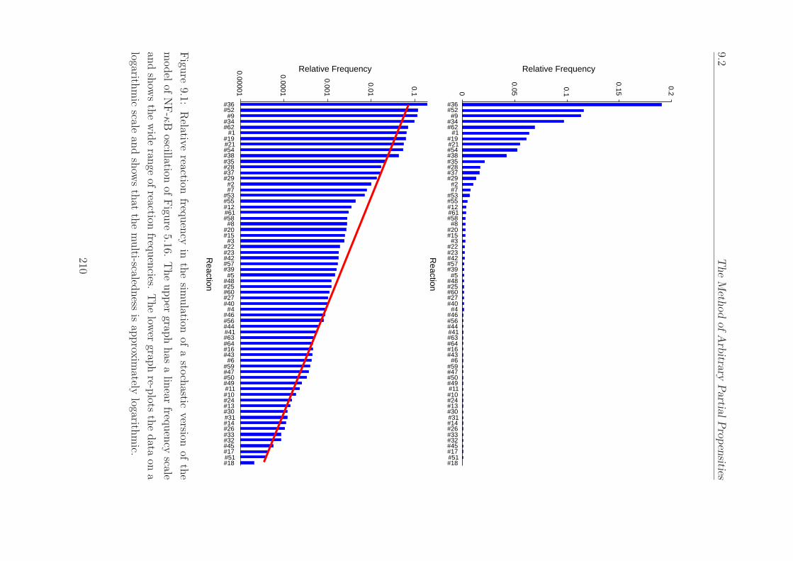
9.2T
he
Meth
od
ofA
rbitra
ryPartia
lP
ropen
sities
0
0.05
0.1
0.15
0.2
#36#52#9
#34#62
#1#19#21#54#38#35#28#37#29
#2#7
#53#55#12#61#58
#8#20#15
#3#22#23#42#57#39#5
#48#25#60#27#40
#4#46#56#44#41#63#64#16#43
#6#59#47#50#49#11#10#24#13#30#31#14#26#33#32#45#17#51#18
Relative Frequency
Reaction
#36#52#9
#34#62
#1#19#21#54#38#35#28#37#29
#2#7
#53#55#12#61#58
#8#20#15
#3#22#23#42#57#39#5
#48#25#60#27#40
#4#46#56#44#41#63#64#16#43
#6#59#47#50#49#11#10#24#13#30#31#14#26#33#32#45#17#51#18
Relative Frequency
Reaction
0.00001
0.0001
0.001
0.01
0.1
Figu
re9.1:
Relative
reactionfreq
uen
cyin
the
simulation
ofa
stoch
asticversion
ofth
e
model
ofN
F-κ
Boscillation
ofFigu
re5.16.
The
upper
graph
has
alin
earfreq
uen
cyscale
and
show
sth
ew
ide
range
ofreaction
frequen
cies.T
he
lower
graph
re-plots
the
data
ona
logarithm
icscale
and
show
sth
atth
em
ulti-scaled
ness
isap
prox
imately
logarithm
ic.
210

The Method of Arbitrary Partial Propensities 9.2
0
0.05
0.1
0.15
0.2
0.25
#6 #3 #8 #9 #10 #1 #12#15 #14 #2 #16 #5 #7 #11 #13 #4
Reaction
Rel
ativ
e F
requ
ency
#6 #3 #8 #9 #10 #1 #12#15 #14 #2 #16 #5 #7 #11 #13 #4
Reaction
Rel
ativ
e F
requ
ency
0.00001
0.0001
0.001
0.01
0.1
1
Figure 9.2: Relative reaction frequency in the simulation of the noise-resistant oscillator
of Figure 5.11. The left graph has a linear frequency scale while the right graph re-plots
the data on a logarithmic scale to show the approximately logarithmic distribution. For
such an optimal ordering of reactions, the average search depth of the ODM corresponds
to the third category, i.e., where the sum of relative frequency reaches 0.5.
in [13] results in many reactions (i.e., those at the end of the chain) not
actually being used at all, hence the ODM does not have to venture too
far into the list of reactions and can thus match the performance of the
NRM. Since the reactions are ordered and the last reactions in the chain
are unused, lengthening the chain by adding more unused reactions has
minimal or no effect on the cost of searching for the reaction to execute.
Note that this beneficial effect is inherent in the NRM because its re-
ordering of the tree at every step automatically places unused reactions far
from the root.
The reasons behind the increase in computational time of the ODM
and NRM as the model size increases, as shown in Figure 1 of [13], are
therefore unclear, since the additional reactions are not active and do not
contribute. Given that the two algorithms apparently scale at the same
rate, it is suspected that the cause of this phenomenon is some unforeseen
common O(M) task, such as storing the system state. Evidence for this
211
9.3 The Method of Arbitrary Partial Propensities
supposition is that in Figure 1 of [13], the DM applied to the same linear
models reveals that the ODM is slightly more than twice as fast across
the range of values plotted; an improvement which is consistent with the
known reduction of the reaction selection from O(M) to O(1) given some
other O(M) cost. A possible amelioration is suggested in Section 9.3.1.
9.3 Optimizations
In this section more detailed analysis of complexity is performed and it is
shown that the NRM outperforms the DM with all but trivial models. It
is further shown that, contrary to the conclusions of [13], the NRM also
outperforms the ODM on non-trivial models. Finally, the Method of Arbi-
trary Partial Propensities (MAPP) is presented and shown to outperform
the NRM on a wide range of biologically plausible instances.
In algorithmic research the goal is usually to reduce the order of com-
plexity of an algorithm and constants are often ignored due to being asymp-
totically unimportant. Depending on the application however, such con-
stants can be highly significant in practice: a division by two of running
time is usually considered worth having. In a practical context, pursuing
a low asymptotic complexity at the expense of a greater complexity in the
useful range of an algorithm is clearly absurd. Hence, in Table 7.1 the rel-
ative time cost of a range of computational operations is defined in order
to better understand the performance of the algorithms.
9.3.1 Optimization 1
The number of reactions in a system is often related in an approximately
linear way to the number of reactants: a reactant usually has one or more
reactions in which it is used ‘constructively’, i.e., linked in some way to
another reactant, plus perhaps one or more reactions in which it is de-
212

The Method of Arbitrary Partial Propensities 9.3
graded. In large systems, however, a reactant is unlikely to react with the
majority of the other reactants. Hence, the number of reactants can be
considered O(M). While the Gillespie algorithm limits the total number
of reactants of any reaction to a maximum of two or three, on the basis
that the collision of more than two molecules at any instant is extremely
unlikely [32, 33, 35], it imposes no theoretical bound on the number or
nature of products. Hence, a general purpose implementation must allow
for reactions with an arbitrary number and combination of products. A
naıve implementation might then have an array of product species for each
reaction, where the size of the array is the total number of species: O(M)
by the previous assumption. This array contains many zeros, but in order
to execute a reaction and update the species, it would be necessary to per-
form a mostly redundant iteration through the product array. This effect
can be repeated when the simulation time-course is updated or output: by
writing out every species instead of only those which have changed, the
algorithm incurs an additional O(M) cost.
The proposed optimization is therefore to have reactions that use a
linked list of products which will usually be much shorter than the full list
of species (typically less than four). The complexity of the execution of a
reaction can then be considered O(1), since this number is not generally
linked to the size of the model. In a similar way, the simulation traces must
be recorded as a series of changes (or a series of reactions) rather than a
series of states.
It is noted there that this problem is common to all algorithms and may
be unavoidable if the data need to be represented as a series of states for
graph plotting or other post-processing. Not all the simulated points are
necessarily plotted, however, hence when the traces are sampled at fixed
time intervals during the simulation, for example, the cost of generating
states from changes in state becomes O(1) relative to M .
213
9.3 The Method of Arbitrary Partial Propensities
9.3.2 Optimization 2
The major computational complexity of the NRM is contained in maintain-
ing the invariant property of the vertically ordered tree. When a value of a
node in the tree is altered by the execution of a reaction, the NRM uses an
update algorithm which applies pairwise swaps of nodes until the vertical
ordering is restored. In [31] the authors describe a SWAP algorithm which
‘swaps the tree nodes ... and updates the index structure’. Two arbitrary
adjacent nodes in the tree have a total of ten internal and external uni-
directional links which must be modified when they are swapped. This is
because each node must know its parent and its children (three links) and
its parent and children must also know it (three more links). This gives six
unidirectional links per node to be swapped, with two links being common,
hence ten in total. Swapping the nodes will therefore involve ten variable
swaps, requiring thirty individual variable assignments. It is noted, how-
ever, that the tree structure itself is constant and it is only the contents of
the nodes that need to be swapped.
The proposed optimization is therefore to have a static tree containing
pointers to reaction structures which hold all the information about the
reaction (reactants, products, rate, putative time etc.). When a reaction
is executed by the NRM, the putative times of its dependent reactions
are updated and their positions in the tree are also updated accordingly.
It is therefore necessary for a reaction to keep a record of its position in
the tree, hence an optimized swap algorithm involves swapping a total of
two variables (a link from the tree node to the reaction and one from the
reaction to the tree node), which require a total of six individual variable
assignments. This optimization thus constitutes a local saving of a factor
of five.
214

The Method of Arbitrary Partial Propensities 9.4
9.3.3 Optimization 3
A further optimization is to re-order the tree without using pair-wise swap-
ping (‘bubbling’), which is not an efficient way of moving a reaction to a
new position (recall the inefficiency of bubble sort). Assuming an updated
reaction has a shorter time than its parent, the optimized technique is to
shift down by one node all the progenitors of the current reaction which
have longer times and to move the current reaction to the position of its
progenitor having the shortest time greater than it. This forms a kind of ro-
tational shift where each movement is an assignment of two variables. The
case of the current reaction having a longer time than one of its children
works in an analogous way: a rotational shift in the opposite direction.
A tree that requires s swaps to be re-ordered, using 6s variable assign-
ments, can thus be re-ordered by s/2 + 1 shifts using only 2s+ 2 variable
assignments. An improvement in all cases is therefore guaranteed, with a
local factor of improvement of between 1.5 and 3.
9.4 The Method of Arbitrary Partial Propensities
The Method of Arbitrary Partial Propensities (MAPP) is designed to over-
come the drawbacks of the NRM and ODM and give good performance for
a range of models on the first run, without pre-ordering (although adap-
tive ordering is beneficial). It is a descendent of the DM, in that it sums
propensities and selects a reaction using a uniformly distributed random
number, however by employing a unique data structure and some of the
optimizations described above it is able to outperform previous algorithms.
The NRM aims to achieve asymptotic O(logM) performance by dy-
namically arranging the reactions in an ordered tree, but suffers a penalty
with models that are not large due to the overhead that this creates. The
ODM seeks to overcome this limitation by statically ordering the reactions
215

9.4 The Method of Arbitrary Partial Propensities
to minimise the search time, but this is only successful for models which
have an overall multiscale property. In fact, both the NRM and ODM rely
on the multiscale property: the advantage of the NRM is limited in the
case that all the reactions have similar speeds because the reactions at the
bottom of the tree must then be brought to the top more frequently.
9.4.1 Details of the MAPP
The MAPP uses a static tree-like data structure of height two, where the
leaf nodes of the tree each contain an array of reaction propensities. The
single parent node (the parent layer) also contains an array, each element
of which is associated with a different leaf (or child) node and contains
the sum of the propensities in the corresponding child. The parent array
has length⌈√
M⌉
and each of its⌈√
M⌉
children contain arrays of length⌈
M/⌈√
M⌉⌉
, such that the total number of array elements in the child
layer is ≥ M . Simply put, the child layer contains all the individual re-
action propensities and the parent layer contains their partial sums - the
partial propensities.3 These sums are therefore arbitrary partial propensi-
ties, since unlike the case of the method of partial propensities presented
in Chapter 8, they do not correspond to any feature of the model.
The sum of the elements of either layer is the total propensity. When the
square root of the number of reactions is not an integer, the total number
of array elements in the child layer will be greater than the number of
reactions. In this case the unused array elements contain zero, although
the value is arbitrary since the algorithm will not consider them. Figure
9.3 illustrates the two layer data structure for M = 11.
The MAPP algorithm is initialized by calculating all the propensities
3This is reminiscent of the Optimized Direct Method proposed in the Appendix of [31], which uses a
binary tree to store propensities. The crucial difference is that the MAPP uses a constant height data
structure, such that the cost of updating the propensities is O(1).
216
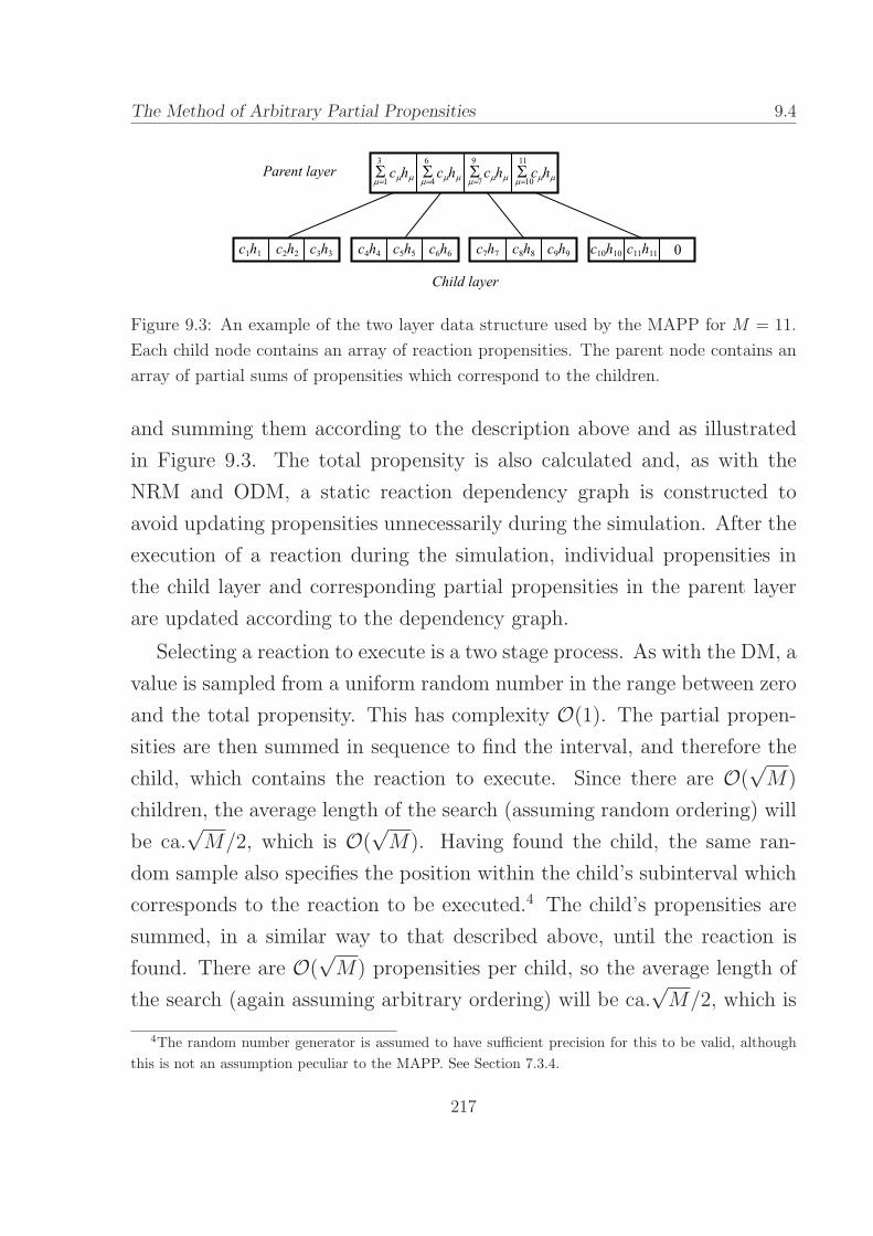
The Method of Arbitrary Partial Propensities 9.4
Figure 9.3: An example of the two layer data structure used by the MAPP for M = 11.
Each child node contains an array of reaction propensities. The parent node contains an
array of partial sums of propensities which correspond to the children.
and summing them according to the description above and as illustrated
in Figure 9.3. The total propensity is also calculated and, as with the
NRM and ODM, a static reaction dependency graph is constructed to
avoid updating propensities unnecessarily during the simulation. After the
execution of a reaction during the simulation, individual propensities in
the child layer and corresponding partial propensities in the parent layer
are updated according to the dependency graph.
Selecting a reaction to execute is a two stage process. As with the DM, a
value is sampled from a uniform random number in the range between zero
and the total propensity. This has complexity O(1). The partial propen-
sities are then summed in sequence to find the interval, and therefore the
child, which contains the reaction to execute. Since there are O(√M)
children, the average length of the search (assuming random ordering) will
be ca.√M/2, which is O(
√M). Having found the child, the same ran-
dom sample also specifies the position within the child’s subinterval which
corresponds to the reaction to be executed.4 The child’s propensities are
summed, in a similar way to that described above, until the reaction is
found. There are O(√M) propensities per child, so the average length of
the search (again assuming arbitrary ordering) will be ca.√M/2, which is
4The random number generator is assumed to have sufficient precision for this to be valid, although
this is not an assumption peculiar to the MAPP. See Section 7.3.4.
217

9.4 The Method of Arbitrary Partial Propensities
O(√M). Hence, selecting a reaction has overall complexity O(
√M).
For every propensity updated, a partial propensity and the total propen-
sity must also be updated. Assuming that the model has average depen-
dency D, updating the propensities and the partial propensities requires
on average 3D operations, which has complexity O(D). Calculating the
incremental time, using Equation 7.9, is O(1), as before. Hence, the overall
asymptotic time complexity of the MAPP is
O(D) +O(√M) (9.2)
.
9.4.2 Comparison of the MAPP, NRM and ODM
To recap, the three algorithms have the following asymptotic complexities.
NRM:
O(D logM); ODM: O(S) + O(D) and MAPP: O(D) + O(√M). M is
the number of reactions in the model, D is the average dependency of the
reactions in the model, S is the average search depth and, in general for a
large model, D < S < M . Note that S is strictly less than M in the case of
a model where the average number of reactions used during the simulation
is > 1. For an ordered model, S ≤M/2.
For unordered models or models which do not benefit from ordering,
O(S) = O(M), hence the MAPP will be faster than the ODM. The relative
performance of these two algorithms with multiscale models will depend
on the ratio of S to√M , i.e., exactly how multiscale it is. By comparison
of Equations 9.1 and 9.2, the model must satisfy the condition S <√M
for the ODM to outperform the MAPP. Note that although the MAPP is
designed to achieve good performance without ordering, its performance
will also benefit from ordering the reactions. The NRM re-orders the reac-
tions at each step during the course of the simulation, so does not benefit
218

The Method of Arbitrary Partial Propensities 9.4
from pre-ordering.
For an ordered multiscale model where S ≤√M but S 6≪
√M , the
asymptotic complexity of the MAPP is O(D) + O(√M) because the se-
lection of the child node will be O(1) (the first child is almost always
chosen since, by definition, the average search depth is less than the par-
tial propensity of the first child), but the selection of the reaction within
the child will not necessarily be speeded up. If S ≪√M , the complex-
ity reduces to O(D) +O(S/√M)) because now the choice of the reaction
within the child is influenced by the ordering. The MAPP will in fact out-
perform the ODM on all models except those very rare cases which satisfy
D ≈ S ≪√M , i.e., those which are extremely multiscale and are heavily
dominated by very few reactions. In such cases the increased overhead of
the MAPP relative to the ODM becomes significant.
In comparing the performances of NRM and MAPP applied to real
model instances, the asymptotic complexities given above are not very
informative, even when the models are large. Since it has been observed
that average reaction dependency, D, in biological models is generally much
less than M , it might be supposed that the NRM will outperform the
MAPP because logM will tend to be less than√M . In real biological
models D scales weakly with M , perhaps somewhere between O(logM)
and O(√M), and the logarithmic term of the NRM is multiplied by D.
The relative performances thus depend on the model being simulated, its
stochasticity and the constants which have so far been omitted from the
asymptotic complexities. With high dependency, such as in the case of the
Colonies of Synchronising Agents model with agent reactions, the NRM
has been shown in Chapter 8 to be less efficient than the ODM. With low
dependency and the typical dependency found in single instances of the
noise resistant oscillator and NF-κB models, experimental results show
that the MAPP is generally faster, but the differences are smaller (see
219

9.4 The Method of Arbitrary Partial Propensities
Figures 9.5, 9.6 and 9.7).
9.4.3 Generalization of the MAPP
So far a data structure has been considered for the MAPP with only two
layers (Figure 9.3), since this is already efficient, but the concept of the
MAPP can be generalised to include an arbitrary number of layers. In
general, increasing the number of layers has the effect of reducing the or-
der of complexity of the algorithm because for n layers, each node containsn√M reactions. The cost of reaction selection is thus reduced and since
n is a constant it can be increased arbitrarily without appearing in the
asymptotic complexity. The effect of increasing n is felt in the cost of up-
dating the partial propensities: a partial propensity on each layer must be
updated for every reaction propensity that changes. n therefore manifests
itself as a multiplier of the average reaction dependency, D.
The minimum number of layers is one, which effectively reduces the
MAPP to the ODM: update cost is O(D) and selection by summation is
O(S), where S ≤M for unordered reactions and S ≤M/2 when they are
ordered.
The maximum number of layers is ⌈log2(M + 1)⌉, which produces the
binary tree structure suggested in the Appendix of [31] (the original op-
timized direct method). Here the cost of updating is proportional to
D ⌈log2 (M + 1)⌉ and the cost of selection is proportional to ⌈log2 (M + 1)⌉(no summation is performed, just a choice between the two alternatives).
It can be seen that the bulk of the cost has shifted from selection to up-
date. The apparent O(D logM) performance might seem ideal, however
in this case the algorithm does not benefit from ordering the reactions and
can not take advantage of multiscale models, as can the other algorithms
considered here. Moreover, the hidden constants and increased memory
requirement (there are as many partial propensities as propensities) make
220

The Method of Arbitrary Partial Propensities 9.5
this configuration less than optimal for practical purposes.
An approximate optimum number of layers is proposed to be
k(M) = log2(M)/ log2 log2(M) (9.3)
such that each node in the tree contains an array of log2 M partial propen-
sities. In this way the summation on each layer of the tree is O(logM).
The cost of updating the tree is then O(kD) and the cost of selection is
O(k logM). This is reminiscent of the complexity of the NRM (O(D) +
O(D log2M)), noting that k is also a function of M but one which grows
very slowly. In practice, for M = 16, k = 2; for M = 1000, k ≈ 3; for
M = 216, k = 4. Hence, for models having D ≈ 4, for example, the MAPP
might be expected to outperform the NRM on models up to 216 reactions
by choosing the number of layers according to Equation 9.3.
9.5 Results
In order to verify the theoretical treatment of the algorithms it is nec-
essary to construct benchmark model instances which demonstrate their
asymptotic scaling and relative performance. Since the motivation of the
present work is the simulation of large biological systems, it is desirable
that the benchmarks be biological in nature. Thus, the models of the
noise-resistant oscillator (NRO) of Figure 5.11 and the oscillatory model
of NF-κB (Figure 5.16) were used as the basis to generate models with in-
creasing complexity. Although both oscillatory in nature, the models have
distinct characteristics: the NRO has few reactions, average dependency
around four, continuous oscillations, few molecules and is very stochastic;
the NF-κB model is much larger, has average dependency around nine,
damped oscillations, large numbers of molecules and is not very stochastic.
Benchmark models were therefore constructed using multiple indepen-
dent instances of the NRO and NF-κB pathways. That is, multiple in-
221

9.5 The Method of Arbitrary Partial Propensities
stances of either the NRO or NF-κB models were included in a single
model file, each instance having species with an appended index and a
unique set of corresponding reactions.
The average dependency within a network of reactions has a significant
effect on the performance of stochastic algorithms used to simulate them,
as was shown in Chapter 8 in relation to the CSA model. It is not clear
how average reaction dependency scales with biological network size so
this was treated as an external parameter. Since the constituent instances
of the benchmark models are independent, the overall average reaction
dependency in the multiple models is the same as the individual case.
Having thus created a set of models with average dependency of (ap-
proximately) four and nine, respectively for NRO and NF-κB, a further
entirely artificial set was created with average dependency equal to one.
This was achieved by creating models containing multiple parallel instances
of reactions of the form
Si → S ′i (9.4)
where for all i = 1 . . .M , Si 6= S ′i, the initial number of molecules of Si is
1000 and the simulation was run for 1000M steps.
The results of preliminary investigations using the benchmark instances
described above are shown in Figures 9.5, 9.6 and 9.7. Figure 9.5 serves to
broadly categorize the models in accordance with theory: the DM is con-
sistently O(M); the ODM is initially good but inevitably becomes O(M);
the MAPP and NRM both have significantly better performance than both
the DM and ODM, with the NRM slightly ahead for the largest models.
With the implemented optimizations and in the unrealistic (trivial) case
of average reaction dependency equal to one, the NRM needs to perform
only one swap to re-order its tree data structure. Above 3000 reactions
the performance of the NRM and MAPP appear to diverge from what is
expected from theory. More evident in Figures 9.6 and 9.7, this is the
222

The Method of Arbitrary Partial Propensities 9.5
result low level memory caching limitations.
For the biological models, below 10 NF-κB systems (below 40 systems
in the case of the NRO), the algorithms seem to scale in accordance with
theory. The DM is the reference with O(M) scaling. The ODM, NRM
and MAPP are similarly efficient for small instance size, but the ODM
progressively drifts towards O(M) as larger instance sizes have reaction
distributions which are less logarithmic. In fact, the average search depth of
the ODM is proportional to the number of parallel instances of the models
in the way shown in Figure 9.4. The NRM and MAPP scale similarly and
at similar levels in the case of the NF-κB models. Although the NRM and
MAPP also scale similarly in the case of the NRO models, the increased
stochasticity gives the MAPP an advantage: the NRM has to constantly
re-order relatively deeper parts of the reaction tree in comparison to the
almost deterministic NF-κB system.
Above 10 (40 for NRO) systems, the performance of the NRM and
MAPP algorithm increasingly reflect the effects of low level memory caching
(i.e., not disk caching). Whereas the times of the NRM might be expected
to flatten relative to the MAPP and eventually drop below it (i.e.,O(logM)
versus O(√M)), both rise with increasing memory use. Importantly, when
these effects start to become significant, the inherently lower memory re-
quirements of the MAPP give it a lead which it maintains thereafter.
A final point to observe is the performance of an ODE solver (lsoda in
Scilab 4.0) relative to the stochastic simulation algorithms. In the case of
the NRO models, all the stochastic simulation algorithms, including the
DM, outperform the deterministic simulation. This is because the NRO
models have low copy numbers of molecules and the stochastic simulation
algorithms have relatively little to do. Moreover, the waveforms contain
a lot of high frequencies (in part resulting from the flat bottoms) so the
ODE solver has to use small time steps. By comparison, the NF-κB mod-
223
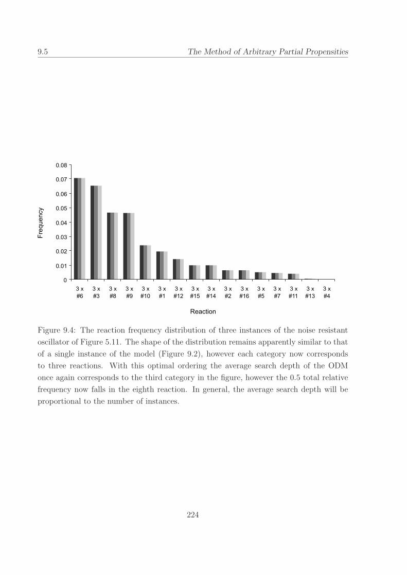
9.5 The Method of Arbitrary Partial Propensities
Figure 9.4: The reaction frequency distribution of three instances of the noise resistant
oscillator of Figure 5.11. The shape of the distribution remains apparently similar to that
of a single instance of the model (Figure 9.2), however each category now corresponds
to three reactions. With this optimal ordering the average search depth of the ODM
once again corresponds to the third category in the figure, however the 0.5 total relative
frequency now falls in the eighth reaction. In general, the average search depth will be
proportional to the number of instances.
224

The Method of Arbitrary Partial Propensities 9.6
els have high copy numbers of molecules and smooth waveforms. While
the stochastic simulation algorithms have to simulate all the molecular in-
teractions, the ODE solver can take advantage of the smoothness and use
long time steps. In the case of the NF-κB models, the ODE solver there-
fore consistently outperforms the stochastic simulation algorithms in the
range of model sizes considered. The trend of the ODE curve seems to
be tending towards O(M), in line with the DM and ODM, presumably as
a result of memory requirements. It seems plausible from this trend that
larger models will favour the performance of the MAPP and NRM.
Figure 9.5: Algorithm scaling with increasing numbers of parallel reactions having average
dependency 1.
225
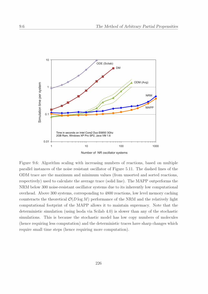
9.6 The Method of Arbitrary Partial Propensities
Figure 9.6: Algorithm scaling with increasing numbers of reactions, based on multiple
parallel instances of the noise resistant oscillator of Figure 5.11. The dashed lines of the
ODM trace are the maximum and minimum values (from unsorted and sorted reactions,
respectively) used to calculate the average trace (solid line). The MAPP outperforms the
NRM below 300 noise-resistant oscillator systems due to its inherently low computational
overhead. Above 300 systems, corresponding to 4800 reactions, low level memory caching
counteracts the theoretical O(D logM) performance of the NRM and the relatively light
computational footprint of the MAPP allows it to maintain supremacy. Note that the
deterministic simulation (using lsoda via Scilab 4.0) is slower than any of the stochastic
simulations. This is because the stochastic model has low copy numbers of molecules
(hence requiring less computation) and the deterministic traces have sharp changes which
require small time steps (hence requiring more computation).
226
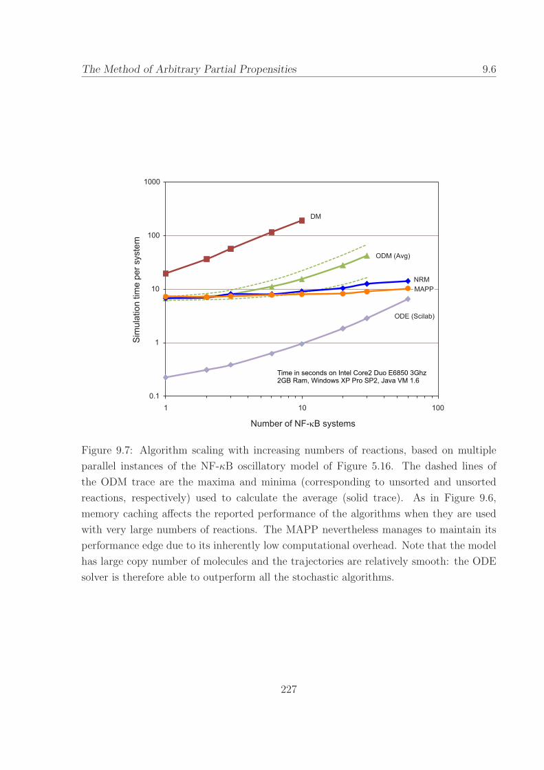
The Method of Arbitrary Partial Propensities 9.6
Figure 9.7: Algorithm scaling with increasing numbers of reactions, based on multiple
parallel instances of the NF-κB oscillatory model of Figure 5.16. The dashed lines of
the ODM trace are the maxima and minima (corresponding to unsorted and unsorted
reactions, respectively) used to calculate the average (solid trace). As in Figure 9.6,
memory caching affects the reported performance of the algorithms when they are used
with very large numbers of reactions. The MAPP nevertheless manages to maintain its
performance edge due to its inherently low computational overhead. Note that the model
has large copy number of molecules and the trajectories are relatively smooth: the ODE
solver is therefore able to outperform all the stochastic algorithms.
227
9.6 The Method of Arbitrary Partial Propensities
9.6 Conclusion
By taking advantage of the observation that reaction dependency in chem-
ically reacting systems tends to be low, the Next Reaction Method [31]
(NRM) is able to improve on the performance of both the Direct Method
(DM) and First Reaction Method (FRM) of [32, 33]. These latter appar-
ently make no assumptions about the system and feature few optimizations.
The NRM uses a tree data structure and a dynamic technique to order the
reactions to thus allows an efficient selection of the next reaction to be ex-
ecuted. For very large systems, the cost of dynamically ordering the active
reactions is offset by not having to search through all the inactive ones.
The authors of [13] made a further observation that some systems are in-
herently multiscale, containing reactions which are used significantly more
frequently than others during the course of a simulation. By applying an
optimal static ordering to these systems it is therefore possible to take ad-
vantage of this property using the simple linear storage structure of the
DM and thus create an Optimised Direct Method (ODM). For certain sys-
tems, the sub-optimal performance of linear storage is more than offset by
the elimination of the costly dynamic ordering of the NRM.
By minimising implementational differences and applying additional
optimizations, it has been possible in this chapter to lay bare the core
performance of the competing algorithms mentioned above. In doing so,
it has also been possible to devise an algorithm which apparently more
closely suits the models of current interest: the Method of Arbitrary Par-
tial Propensities (MAPP). This has been achieved by a balanced strategy
which acknowledges the existence of multiscale systems and the benefits
of tree structures for data retrieval: the algorithm includes both, without
completely relying on either. This is clearly a practical approach.
There is scope for improvement, but the law of diminishing returns
228

The Method of Arbitrary Partial Propensities 9.6
prevails. Re-ordering of the reactions between runs of multiple simulation
runs has already been implemented and is computationally cheap, however
it has been found that the gains are minimal. A further gain may be
achieved by adaptive re-ordering during simulation runs: not at every step
like the NRM but on a timescale that reflects a slower trend of reaction
dependency. It is noted, however, that in the worst case there may not be
such a trend.
229

9.6 The Method of Arbitrary Partial Propensities
230

Chapter 10
Fourier analysis of stochastic
simulations
Some the work presented in this chapter was originally published in the poster
S. Sedwards and A. Csikasz-Nagy (2008) Characterization of mutants by Fourier analysis of
stochastic simulations of yeast cell cycle, 9th International Conference of Systems Biology,
Goteborg, Sweden.
The choice of a discrete paradigm to represent chemically reacting systems,
such as those presented in Chapters 3 to 6, has the potential to investigate
biology in the most precise way. For example, using the techniques of
model checking (e.g., [23]) it is possible to define exact logical properties
(or exact probabilities in the case of probabilistic model checking [56, 89])
of a given system. In the case of paradigms which have the chemical master
equation (CME) at their root, it is also conceivable to solve the CME to
give a description to arbitrary precision of the distribution of a species at
a given time point. It is often the case, however, that non-trivial biological
systems have an intractably large state space, rendering model checking
impractical. Solving the master equation also has drawbacks, especially
in the case of systems which exhibit oscillatory behaviour: the oscillations
are not necessarily evident in the distribution (e.g., see Figure 10.2).
231
10.1 Fourier analysis of stochastic simulations
Motivated by the above, an analysis technique based on Fourier transfor-
mation is presented. By transforming the time series produced by stochas-
tic simulation into the frequency domain, it is possible to characterise the
behaviour of both oscillatory and non-oscillatory systems. Moreover, this
technique reveals more information about the system than is possible to
(easily) extract from deterministic simulations.
In what follows it is assumed that the reader is familiar with the notions
of stochastic simulation presented in Chapter 7. It is also assumed that
the reader has a basic familiarity with analysis and statistics. While no
deep theoretical treatment is given, some of the presented methods involve
advanced concepts not likely to be found in introductory textbooks. [54] is
a good reference, but otherwise it is recommended that the reader perform
an Internet search on specific topics of interest.
10.1 Average behaviour
While a single stochastic simulation run often has an apparent charac-
teristic behaviour, such behaviour may have little statistical significance
relative to the total space of possible trajectories. In order to draw general
conclusions about the model it is thus necessary to characterise some kind
of average trajectory, as might be realised by the deterministic simulation
of ordinary differential equations. A simplistic approach to averaging time
series of multiple stochastic simulation runs does not produce an average
trajectory, however: the instantaneous phase shift between simulations is
a random variable, hence oscillatory behaviour of summed time series will
tend to disappear with increasing numbers of cycles. An example of this
effect is shown in Figure 10.1. While there may still be evident oscillation,
this is not in general the case and information will be lost to the averaging
process.
232

Fourier analysis of stochastic simulations 10.2
0 50 100 150 200 250
050
100
200
Time
Num
ber
of m
olec
ules
pA
pR
0 50 100 150 200 250
050
100
150
200
250
Time
Ave
rage
no.
of m
olec
ules
pA
pR
Figure 10.1: The left graph shows typical plots of proteins pA and pR of the noise-resistant
oscillator [84] (see Figures 5.10 and 5.11). The right graph shows average plots of pA and
pR, based on 100 simulation runs. The lack of phase stability in the stochastic time series
causes the amplitude of oscillations to diminish in the average plots.
While the average gained in this way appears to conceal information
about the time evolution of the system, it gathers information about the
distribution of trajectories at given time points. This distribution approxi-
mates a solution to the chemical master equation that describes the system.
Examples of such distributions are shown in Figure 10.2 for two species and
two time points of the noise resistant oscillator model of [84] as shown in
Figures 5.10 and 5.11. The significant observation here is that these dis-
tributions do not reveal the nature of the observed oscillatory behaviour
of a typical trajectory.
10.2 The Fourier transform
The forward Fourier transform is a linear transformation from the time
domain to the frequency domain:
X(f) =
∫ +∞
−∞x(t)e−j2πftdt (10.1)
233

10.2 Fourier analysis of stochastic simulations
time = 200 time = 212
0 50 100 150 200 250
0.00
0.04
0.08
0.12
Value of pA
Pro
babi
lity
0 50 100 150 200 250
0.00
0.04
0.08
0.12
Value of pA
Pro
babi
lity
0 50 100 150
0.00
0.02
0.04
0.06
Value of pR
Pro
babi
lity
0 50 100 150
0.00
0.02
0.04
0.06
Value of pR
Pro
babi
lity
Figure 10.2: Sampled distributions of proteins pA and pR of the noise-resistant oscillator
[84] (see Figures 5.10 and 5.11) evaluated at time = 200 and time = 212. Each plot
is based on samples taken from 10000 simulation runs. Despite being separated by half
the period of oscillation, there is little to distinguish the distributions at the two time
points since the mode of oscillation is equally robust at both. Moreover, the existence of
oscillation is not revealed by such distributions.
234

Fourier analysis of stochastic simulations 10.2
By evaluating this integral for a function of time (i.e., x(t)), it is possible
to find a function of frequency, X(f), which is a frequency spectrum that
exactly describes x(t). Since the transformation is linear, no information
is gained or lost, however the representation of the information may be
more intuitive or compact in the frequency domain. In particular, systems
having oscillatory behaviour are often more conveniently described in the
frequency domain. An example is shown graphically in Figure 10.3, where
it is assumed that the time course extends to infinity in the positive and
negative time directions. By comparison, the two spectral lines (plus their
corresponding phase components, here equal to zero) are a complete finite
description of the infinite time series. Of course, the frequency axis also
continues to positive (and negative) infinity, but it is only necessary to
represent a finite segment of it to completely describe the infinite time
course.
0
-1.5
Time
Am
plitu
de
1 2
-0.5
0.5
1.5
0
0.0
Frequency
Am
plitu
de
0.4
0.8
2 4 6 108
Figure 10.3: Time and frequency domain representations of x(t) = sin(2πt) + sin(4πt).
In the case of the function of time given in Figure 10.3 it is possible apply
the Fourier transfom (Equation 10.1) and derive an analytical solution:∫ +∞
−∞(sin(2πt) + sin(4πt))e−j2πftdt = δ(f − 1) + δ(f − 2) (10.2)
235

10.3 Fourier analysis of stochastic simulations
where δ(·) is the Kronecker delta function (δ(d) = 1 for d = 0, 0 other-
wise. See, e.g., [54]). As expected, the result is a function which gives two
spectral peaks and contains no imaginary part because there is no phase
difference between the components.
For this contrived example, while there is an evident simplification of
the description of the behaviour when it is represented graphically, it can
be argued that the time and frequency domain representations are equiv-
alently compact and intuitive. In the case of biological systems described
by non-linear differential equations (or a stochastic alternative), no such
explicit functional description of the time course usually exists. What is
often available are the (discrete) time courses of simulations and possibly
also the corresponding experimental time courses.
The nature of experimental data is thus discrete, requiring that the dis-
crete Fourier transform (DFT, Equation 10.3) is used to transform them.
The DFT is also a linear transformation from the time domain to the fre-
quency domain for which an inverse transformation is defined. A common
application of the DFT is the removal of noise. With sufficient data it
is possible to distinguish the noise from the principal signal by Fourier
decomposition of the time series using the DFT, as illustrated in Figure
10.4. By deleting the unwanted part of the frequency spectrum and ap-
plying the reverse transformation it is then possible to recover (a better
approximation to) the principal signal.
The time courses resulting from the stochastic simulation of biological
models have arbitrary shape and arbitrary amounts of noise. Some of this
noise may be considered an inherent part of the model, i.e., correlated noise,
whereas other noise may give no insight about the model. In Section 10.4
a new technique using Fourier analysis is introduced as a means to usefully
characterise the behaviour observed in stochastic simulation traces.
236
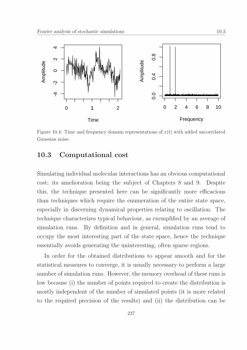
Fourier analysis of stochastic simulations 10.3
0
Time
Am
plitu
de
11 2
-4-2
02
4
0
0.0
Frequency
Am
plitu
de
2 4 6 8 10
0.4
0.8
Figure 10.4: Time and frequency domain representations of x(t) with added uncorrelated
Gaussian noise.
10.3 Computational cost
Simulating individual molecular interactions has an obvious computational
cost; its amelioration being the subject of Chapters 8 and 9. Despite
this, the technique presented here can be significantly more efficacious
than techniques which require the enumeration of the entire state space,
especially in discerning dynamical properties relating to oscillation. The
technique characterizes typical behaviour, as exemplified by an average of
simulation runs. By definition and in general, simulation runs tend to
occupy the most interesting part of the state space, hence the technique
essentially avoids generating the uninteresting, often sparse regions.
In order for the obtained distributions to appear smooth and for the
statistical measures to converge, it is usually necessary to perform a large
number of simulation runs. However, the memory overhead of these runs is
low because (i) the number of points required to create the distribution is
mostly independent of the number of simulated points (it is more related
to the required precision of the results) and (ii) the distribution can be
237

10.4 Fourier analysis of stochastic simulations
stored cumulatively. As a stochastic process, it is conceivable that succes-
sive simulation runs visit the same states, thus perhaps being inefficient
in comparison to enumeration. In practice, the total number of points
generated by all simulation runs is far fewer than the entire state space.
Formalisations of the relationships between state space, number of simu-
lations and the convergence of distributions and measures remain open,
however an illustration of convergence is shown in Figure 10.5.
Having performed the simulation runs it is necessary to transform the
data according to the DFT given in Equation 10.3. This is achieved by
applying a so-called fast Fourier transform (FFT) algorithm, which gen-
erally have asymptotic complexity Θ(N logN), where N is the number of
sampled points. There is not a single most efficient algorithm for arbitrary
N , however it is possible to achieve the given asymptotic complexity by
choosing the algorithm most appropriate for a given value (see [27] for a
review). Since N is generally less than the number of points in a simulation
run, the discrete Fourier transformation does not add significantly to the
overall computational burden.
10.4 Statistical measures over DFT spectra
Multiple simulation runs are made having identical initial conditions and
length (in simulated time) and the resulting time series are converted to
frequency spectra using a discrete Fourier transformation:
fω =N−1∑
n=0
xne− 2iωn
N (10.3)
where fω is the ωth frequency component and xn is the nth time sample
of a given molecular species. Stochastic simulations based on a variant of
the Gillespie algorithm produce time series having irregular time spacing
between points, hence to apply Equation 10.3 it is necessary to sample the
238

Fourier analysis of stochastic simulations 10.4
DFT of 100 cycles. DFT of 400 cycles.
DFT of 12800 cycles. Convergence with increasing cycles.
Figure 10.5: Convergence of statistical measures relating to stochastic simulations of the
budding yeast cell cycle model of Figure 5.21. The three spectra demonstrate increasing
smoothness and illustrate the convergence of µ, ρ1 and ρ2 with increasing number of
simulated cycles.
239

10.4 Fourier analysis of stochastic simulations
stochastic time series at regular time intervals. The method adopted is to
choose xn = xt | max(t ≤ n δt), where xt is the simulation point having
value x at time t and δt is the chosen sampling time step. That is, the
value of species at the time less than or equal to the required sample time.
The result of the DFT is N complex numbers per simulation run, con-
taining amplitude and phase information for each of the N frequencies.
Since these frequencies correspond between runs (by definition), the data
can be combined to give a distribution (runs will be different from each
other by virtue of the stochasticity). Note, however, that it is not sufficient
to simply add the complex numbers. Since the DFT is a linear transforma-
tion, adding the transformed data is equivalent to performing a transform
on the sum of the time series. The result would suffer the same limitations
described in Section 10.1 and shown in Figure 10.1.
The solution is not to add the raw complex data but to add the moduli
of the spectral data.
The spectra created in this way form distributions which characterize
the observed behaviour in a compact form. Figure 10.6 shows typical re-
sults, comparing the spectra of deterministic and stochastic simulations of
the noise resistant oscillator of [84] (the model is shown in Figures 5.10
and 5.11). Note in particular how high frequency components of the de-
terministic spectrum are not evident in the stochastic spectrum, being lost
in the noise. This behaviour is typical and is an interesting result in itself.
In Section 10.5 Fourier decomposition of stochastic simulations are used to
classify the viability of budding yeast mutants [91]. Typical distributions
of CycBT , relative cell mass and SK (Cdc20A in the case of Mutant 2)
for wild type and three mutant yeast strains are shown in Figures 10.11,
10.12, 10.13 and 10.14. The corresponding DFT spectra from deterministic
simulations are also shown for comparison with wild type and mutant 3.
The key point to observe is that there is qualitatively little to discern the
240

Fourier analysis of stochastic simulations 10.4
Figure 10.6: Comparison of DFT spectra of stochastic and deterministic simulations of
protein A (pA) of the noise resistant oscillator of [84]. Note that (i) high frequency
components of the deterministic spectrum are not evident in the stochastic spectrum
and (ii) the ‘mass’ of the deterministic spectral peaks is distributed in the noise of the
stochastic spectrum. A comparison of typical time series is inset.
241

10.4 Fourier analysis of stochastic simulations
deterministic spectra of wild type and mutant 3, yet mutant 3 is known
to be the least viable [80, 49, 85]. The difference is clearly shown in the
stochastic spectra, demonstrating value of the stochastic simulation and
this technique.
10.4.1 Statistical measures
Once spectra have been created, it is possible to define statistical measures
which characterise them. Three such measures are introduced here and
defined as follows:
ρ1 = log2(max(f1..N−1)/〈f1..N−1〉) (10.4)
ρ2 = σ(f1..N−1)/〈f1..N−1〉 (10.5)
ρ3 = sup|F 10..N−1 − F 2
0..N−1| (10.6)
where 〈·〉 denotes the expected value of its argument, σ(·) denotes the
standard deviation of its argument and sup| · | is the supremum of the
absolute values of its argument. F 1 and F 2 are the cumulative distributions
of the empirical distributions given as f1 and f2. Note that
• ρ1 and ρ2 are independent measures of robustness of behaviour: values
decrease to 0 with increasing stochasticity.
⊲ ρ1 is the maximum of the distribution divided by the mean (ex-
cluding µ, the zero frequency component, which is the mean of
the time series).
⊲ ρ2 is the coefficient of variance of the distribution (excluding µ).
• ρ3 is a relative measure, measuring the difference between two distri-
butions.
⊲ ρ3 is the Kolmogorov-Smirnov statistic, with values between 0
and 1, where 0 indicates no difference.
242

Fourier analysis of stochastic simulations 10.5
⊲ ρ3 can be seen to define a space of phenotype which can be applied
to compare models, mutants or stochastic algorithms.
Figure 10.7 demonstrates the use the technique in comparing models of
NF-κB oscillation.
10.5 Fourier analysis of budding yeast mutants
The cell cycle of budding yeast has been thoroughly modelled and simu-
lated using differential equations (e.g., [82]) but much less so using stochas-
tic techniques. The budding yeast cell cycle models are particularly so-
phisticated, with one of the latest being able to accurately represent the
behaviour of more than 100 mutant strains [24]. Using a simplified model
adapted from [82], shown diagrammatically in Figure 10.8 and as a sim-
ulator script in Figure 5.21, the proof of concept of a new technique to
classify the viability of mutants using Fourier analysis applied to stochas-
tic simulations is presented.
Typical deterministic traces are shown in Figure 10.10, which includes
the change in relative mass for reference. Typical stochastic traces for
the same model are shown in Figure 10.10. The stochastic model was
derived from the differential equation model by expanding the differen-
tial equations into corresponding creation and consumption reactions, in
accordance with the reaction scheme. While the goal is to create a set of el-
ementary reactions from the ODEs, some of the reactions in this model use
Michaelis-Menten kinetics and Hill functions and do not contain sufficient
information to make an exact conversion. Moreover, the model uses alge-
braic equations to balance mass and model fast equilibria. These functions
and equations were used without modification, but advisedly.
The three statistical measures define in Section 10.4.1 are used to cat-
egorize the viability of wild type and mutant varieties of budding yeast.
243

10.5 Fourier analysis of stochastic simulations
Parameters from literature New measured parameters
← ρ3 = 0.09→
↑ρ = 0.035
↓↑ Newly inferred parameters
ρ3 = 0.088→
Figure 10.7: DFT spectra and associated statistical measures of NF-κBn oscillation using
the model given in Figure 5.16 and three parameter sets. The spectrum on the left
features parameters taken from the literature, while that in the top right uses parameters
obtained from new measurements. The bottom right spectrum uses parameters inferred
from the raw measured data using a new algorithm [58]. The values of ρ3 show that the
two parameter sets obtained from the new measurements are closer to each other than
either of them are to the parameters obtained from the literature.
244

Fourier analysis of stochastic simulations 10.6
Figure 10.8: The simplified generic model of budding yeast cell cycle. Dashed lines
indicate enzymatic action. Active forms of species are contained in stellated ovals.
Overall viability of three mutant strains in comparison to wild type is
shown in Figure 10.15. The theoretical results agree well with the experi-
mental results relating to the same mutants (e.g., [79, 80]). Note that ρ1
and ρ2 increase with decreasing viability, while ρ3 decreases.
10.6 Prospects
A technique based on Fourier decomposition has been presented which is
able to extract useful information contained in stochastic simulation time
245
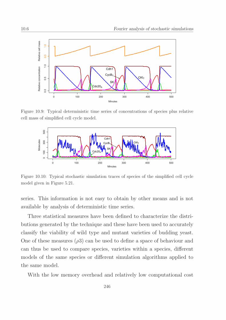
10.6 Fourier analysis of stochastic simulations
Figure 10.9: Typical deterministic time series of concentrations of species plus relative
cell mass of simplified cell cycle model.
Figure 10.10: Typical stochastic simulation traces of species of the simplified cell cycle
model given in Figure 5.21.
series. This information is not easy to obtain by other means and is not
available by analysis of deterministic time series.
Three statistical measures have been defined to characterize the distri-
butions generated by the technique and these have been used to accurately
classify the viability of wild type and mutant varieties of budding yeast.
One of these measures (ρ3) can be used to define a space of behaviour and
can thus be used to compare species, varieties within a species, different
models of the same species or different simulation algorithms applied to
the same model.
With the low memory overhead and relatively low computational cost
246
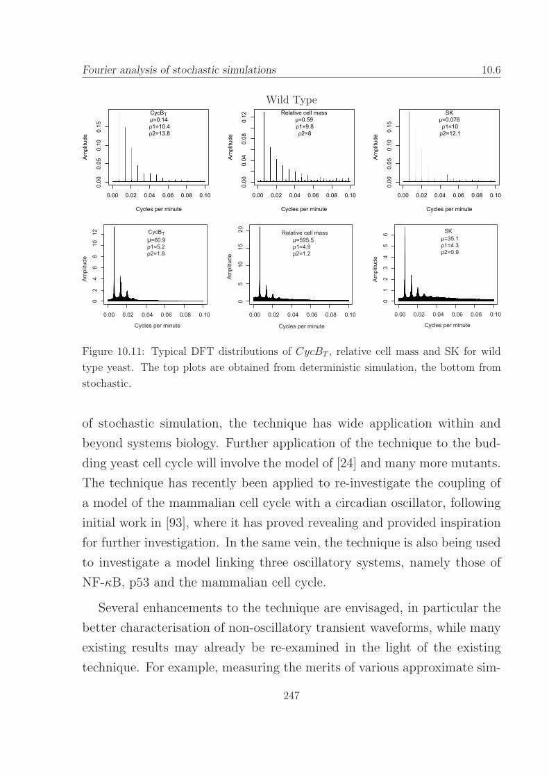
Fourier analysis of stochastic simulations 10.6
Wild Type
Figure 10.11: Typical DFT distributions of CycBT , relative cell mass and SK for wild
type yeast. The top plots are obtained from deterministic simulation, the bottom from
stochastic.
of stochastic simulation, the technique has wide application within and
beyond systems biology. Further application of the technique to the bud-
ding yeast cell cycle will involve the model of [24] and many more mutants.
The technique has recently been applied to re-investigate the coupling of
a model of the mammalian cell cycle with a circadian oscillator, following
initial work in [93], where it has proved revealing and provided inspiration
for further investigation. In the same vein, the technique is also being used
to investigate a model linking three oscillatory systems, namely those of
NF-κB, p53 and the mammalian cell cycle.
Several enhancements to the technique are envisaged, in particular the
better characterisation of non-oscillatory transient waveforms, while many
existing results may already be re-examined in the light of the existing
technique. For example, measuring the merits of various approximate sim-
247

10.6 Fourier analysis of stochastic simulations
Mutant 1: CKI deleted (sic1∆)
Figure 10.12: Typical DFT distributions of CycBT , relative cell mass and SK for sic1∆
mutant.
Mutant 2: CKI & SK deleted (cln1∆, cln2∆, cln3∆, sic1∆)
Figure 10.13: Typical DFT distributions of CycBT , relative cell mass and Cdc20A for
cln1∆, cln2∆, cln3∆, sic1∆ mutant.
ulation algorithms to verify and ascertain the quality of their approxima-
tion.
248

Fourier analysis of stochastic simulations 10.6
Mutant 3: Cdh1 deleted (cdh1∆)
Figure 10.14: Typical DFT distributions of CycBT , relative cell mass and SK for cdh1∆
mutant. The top plots are obtained from deterministic simulation, the bottom from
stochastic.
Figure 10.15: Total measures of viability, using all modelled species, for wild type and
three mutant yeast strains.
249

10.6 Fourier analysis of stochastic simulations
250

Chapter 11
Conclusions
The widespread availability of high computational power and the sequenc-
ing of the human and other genomes has seen an explosion in computa-
tional and systems biology research. It is believed that such power can
be applied to the vast repositories of biological data in order to advance
biological and medical science. The data has been gathered over many
generations of scientists and much of the knowledge is unstructured. In
order to gain inference from the data using computers it will therefore be
necessary to re-interpret it in the context of formal models, such as that
of Membrane Systems.
This thesis has presented two new classes of models of Membrane Sys-
tems, tailored to represent simple and hierarchical biochemical systems.
The underlying formalisms are intuitive to non-experts and have a wealth
of existing technical results for reference, as well as active ongoing research.
Several results have been presented which extend the corpus and thus aid
the understanding of biology. The implementations of these models em-
ploy the concept of multiset rewriting controlled by a stochastic simulation
algorithm. Two simulators and their associated languages have been cre-
ated, one of which, Cyto-Sim, has been presented in detail with many
examples. To ameliorate the computational complexity of stochastic simu-
251

11.0 Conclusions
lation, two new state of the art simulation algorithms have been presented
here. Finally, a new technique based on Fourier analysis was presented
which extracts useful information from stochastic simulations.
Membrane Systems with Peripheral Proteins
In Chapter 3 a model of membrane systems with objects attached to
both sides of the membranes was presented: a Ppp system. The model
is equipped with operations that can rewrite floating objects and move
objects between regions depending on the attached objects. Qualitative
properties of the Ppp system model were investigated, such as configuration
reachability in relation to the use of cooperative or non-cooperative evolu-
tion and transport rules and in the contexts of free- and maximal-parallel
evolution. It was proved that when the system works with free parallel
evolution, the reachability of a configuration or of a certain protein mark-
ing can be decided. It was also shown that when the system works with
maximal parallel evolution the reachability of configurations becomes an
undecidable property for the case of non-cooperative evolution rules and
cooperative membrane rules. The property remains decidable, however,
for systems using non-cooperative evolution rules and simple membrane
rules and for systems using only membrane rules. An interesting problem
remains open: the decidability of reachability in the case of systems us-
ing non-cooperative evolution rules, non-cooperative membrane rules and
maximal-parallel evolution.
252
Conclusions 11.0
Membrane Systems with Peripheral and Integral Pro-
teins
In Chapter 4 a model of membrane systems was presented with objects
integral to the membrane and objects attached to either side of the mem-
brane: a Ppi system. Operations were presented that can rewrite floating
objects conditional on the existence of integral and attached objects and
other operations were presented that facilitate the interaction of floating
objects with integral and attached objects. With these it was shown that
it is possible to model in detail many real biochemical processes occurring
in the cytoplasm and in the cell membrane.
Evolutions of the system are obtained using an enhancement of the
Gillespie algorithm and in the second part of the chapter a noise-resistant
circadian oscillator and the G-protein cycle mating response of Saccha-
romyces cerevisiae were modelled using Cyto-Sim, the simulator presented
in Chapter 5.
Cyto-Sim
The implementation of the Ppp system and Ppi system models, Cyto-Sim,
was described in detail in Chapter 5, including its syntax and many ex-
amples. Cyto-Sim is a tool which has been developed to provide efficient
stochastic simulations of biological processes in compartments, using an
intuitive representation of the underlying formal model. The explicit mod-
elling of compartments and membranes facilitates the construction of mod-
els by composing instances of the variously defined parts, making them
compact and transparent. The simulation engine is based on Markov Chain
Monte Carlo techniques and can be used at arbitrary and mixed levels of
abstraction; micro- and macroscopic biological processes can thus be sim-
253

11.0 Conclusions
ulated using arbitrary kinetic laws best suited to each defined interaction.
It was noted in Chapter 5 that the use of hierarchical compartments has
wide application in biological modelling and in other fields, while the way
in which membranes are modelled in Cyto-Sim is specifically aimed at
molecular cell biology. For maximum utility, Cyto-Sim also accepts mod-
els defined as Petri net matrices and SBML and exports to SBML and
Matlab.
Colonies of Synchronizing Agents
A new paradigm designed to model complex, hierarchical systems called
Colonies of Synchronizing Agents (CSA) was presented and explored in
Chapter 6. Inspired by the intracellular and intercellular mechanisms in
biological tissues, the model is based on a multiset of agents, where each
agent has a local state stored in the form of a multiset of atomic objects.
Hence a CSA can be seen as a multiset of multisets updated by a set of
global multiset rewriting rules either independently or synchronously with
another agent.
The model was first defined then its computational power was studied,
considering the trade-off between internal rewriting and agent synchro-
nization. The dynamic properties of CSAs was also investigated, including
behavioural robustness with respect to the loss of an agent or rule and
safety of synchronization.
Several prospective enhancements to the theoretical model were pro-
posed and primary among these is the addition of space to the colony:
agents have two associated triples corresponding to their position and ori-
entation in space and new rules have the ability to modify these dependent
on distance. Other biologically-inspired primitives considered include agent
division (mitosis) and agent death (apoptosis).
254

Conclusions 11.0
CSAs have been independently described as an ‘elegant model’ and it is
clear that it has many applications related to biology and other complex
systems. One such, not detailed in this document, is described in A Logical
Characterization of Robustness, Mutants and Species in Colonies of Agents
[60], which defines formal ways to characterise fundamental biological con-
cepts using the basic CSA model.
The Method of Partial Propensities
In solving a problem specific to the implementation of Colonies of Syn-
chronizing Agents, a simple method was devised that has utility and wider
application: the Method of Partial Propensities. By partitioning the simu-
lation algorithm along the lines which generate the complexity, it is possible
to significantly ameliorate it and improve on the performance of benchmark
algorithms. The methods presented in Chapter 8 may also be relevant to
other hierarchical stochastic formalisms, such as those based on process
algebra, where complexity derives from combinatorial effects.
The Method of Arbitrary Partial Propensities
By applying some of the ideas of Chapter 8 to more general chemically
reacting systems, it was possible to introduce the Method of Arbitrary
Partial Propensities in Chapter 9; an algorithm which improves on the
performance of the current benchmark, the Next Reaction Method (Section
7.3.2). In order to give the comparison the maximum validity, Chapter 9
also introduced a number of optimisations for the NRM which aimed to
minimise implementational differences between the algorithms.
255

11.1 Conclusions
Fourier analysis
In Chapter 10 a novel and promising analysis technique based on Fourier
decomposition was presented. The technique is able to extract useful infor-
mation from the time series created by stochastic simulation. The informa-
tion so obtained is not easy to obtain by other means and is not available
by analysis of deterministic time series.
Three statistical measures were defined to characterise the distributions
generated by the technique and these were used to characterise the viability
of varieties of budding yeast. One of these measures can be used to define
a space of behaviour and has broad application: it can be used to compare
species, varieties within a species, different models of the same species or
simulation algorithms applied to a single model.
11.1 Prospects and open problems
While the Ppp system model has already been extended to include integral
proteins, becoming a Ppp system, other biologically-inspired operations may
be introduced, such as fission and fusion of regions, all still dependent on
the objects attached to the membranes. On the other hand, the CSA
paradigm might be a more appropriate framework for these, since fission,
i.e. agent division, already exists in the CSA implementation. It would
be relatively simple to implement a fusion operation, with the interesting
prospect of then exploring fission and fusion with space.
A more fruitful line of research with the Ppp system and Ppi system
models is probably their application to the wealth of biological problems
available from the literature which have so far only been explored in the
context of a continuous paradigm via ordinary differential equations. For
example, using Cyto-Sim, which can often import existing models unal-
256

Conclusions
tered, it would be possible to gain new insight by applying the techniques
of Fourier analysis presented in Chapter 10.
With the addition of the features already in prospect for the CSA model,
it will be interesting to extend the investigation and proofs to identify fur-
ther classes of CSAs demonstrating robustness and having decidable prop-
erties. Moreover, it would be interesting to link such theoretical classes
with observed robustness in real biological colonies, such as embryos, tis-
sues, tumours and the immune system. In this way it might be possible to
gain useful insight about important aspects of biology.
The method of partial propensities (MPP) offers a considerable improve-
ment over standard stochastic simulation algorithms applied to the CSA
model. This improvement mostly concerns the amelioration of the effects
of agent reactions, however the internal reactions of the same model may
constitute a difficult computational task in themselves. The method of
arbitrary partial propensities (MAPP) has been shown to be effective for
these types of reactions and so may profitably be incorporated in the MPP.
The MAPP, being highly optimised already, seems to offer limited scope
for further optimisation. Plenty of scope exists, however, for its application
to biological systems and in particular to large biological systems.
With the low overhead and relatively low computational cost of stochas-
tic simulation, Fourier analysis of stochastic simulations seems to have wide
application within and beyond systems biology. Further application to the
budding yeast cell cycle and several enhancements to the technique are
in prospect (e.g., better characterisation of non-oscillatory, transient wave-
forms), while it is envisaged that many existing results and techniques may
be re-examined in the light of the new technique. For example, measuring
the merits of various approximate simulation algorithms.
257

Conclusions
258

Bibliography
[1] H. Abelson, D. Allen, D. Coore, C. Hanson, G. Homsy, T. F. Knight,
R. Nagpal, E. Rauch, G. J. Sussman, and R. Weiss. Amorphous Com-
puting. Communications of the ACM, 43, 2000.
[2] B. Alberts, A. Johnson, J. Lewis, M. Raff, K. Roberts, and P. Walter.
Molecular Biology of the Cell. Garland Science, 4 edition, 2002.
[3] A. Alhazov. Minimizing Evolution-Communication P Systems and EC
P Automata. New Generation Computing, 22, 2004.
[4] M. Ben-Ari, A. Pnueli, and Z. Manna. The temporal logic of branching
time. Acta Informatica, 20, 1983.
[5] F. Bernardini, R. Brijder, G. Rozenberg, and C. Zandron. Multiset-
based self-assembly of graphs. Fundamenta Informaticae, 75, 2007.
[6] F. Bernardini and M. Gheorghe. Population P Systems. Journal of
Universal Computer Science, 10, 2004.
[7] F. Bernardini and M. Gheorghe. Cell communication in tissue P sys-
tems: Universality results. Soft Computing, 9, 2005.
[8] R. Brijder, M. Cavaliere, A. Riscos-Nunez, G. Rozenberg, and
D. Sburlan. Membrane Systems with Marked Membranes. In Proceed-
ings of the First Workshop on Membrane Computing and Biologically
259

BIBLIOGRAPHY
Inspired Process Calculi (MeCBIC 2006), volume 171 of Electronic
Notes in Theoretical Computer Science, pages 25–36, July 2007.
[9] Y. Cao, D. T. Gillespie, and L. R. Petzold. Avoiding negative popu-
lations in explicit Poisson tau-leaping. Journal of Chemical Physics,
123, 2005.
[10] Y. Cao, D. T. Gillespie, and L. R. Petzold. Multiscale stochastic
simulation algorithm with stochastic partial equilibrium assumption
for chemically reacting systems. Journal of Computational Physics,
206(2):395–411, 2005.
[11] Y.. Cao, D. T. Gillespie, and L. R. Petzold. The slow-scale stochastic
simulation algorithm. Journal of Chemical Physics, 122, 2005.
[12] Y. Cao, D. T. Gillespie, and L. R. Petzold. Efficient stepsize selection
for the tau-leaping simulation method. Journal of Chemical Physics,
124, 2006.
[13] Y. Cao, H. Li, and L. R. Petzold. Efficient formulation of the stochastic
simulation algorithm for chemically reacting systems. J. Chem. Phys.,
121:4059–4067, 2004.
[14] L. Cardelli. Brane calculi: Interactions of biological membranes. In
V. Danos and V. Schachter, editors, Proceedings of Computational
Methods in System Biology 2004, volume 3082 of Lecture Notes in
Computer Science. Springer-Verlag, Berlin, 2005.
[15] L. Cardelli and Gh. Paun. An universality result for a (mem)brane
calculus based on mate/drip operations. In M.A. Gutierrez-Naranjo,
Gh. Paun, and M.J. Perez-Jimenez, editors, Proceedings of the ESF
Exploratory Workshop on Cellular Computing (Complexity Aspects),
260

BIBLIOGRAPHY
volume 17 of International Journal of Foundations of Computer Sci-
ence, pages 49–68. World Scientific Publishing Company, 2006. Fenix
Ed., Seville, Spain.
[16] M. Cavaliere. Evolution-Communication P systems. In Gh. Paun,
G. Rozenberg, A. Salomaa, and Zandron C., editors, Proceedings of
the International Workshop of Membrane Computing, volume 2597 of
Lecture Notes in Computer Science. Springer-Verlag, Berlin, 2003.
[17] M. Cavaliere, S. N. Krishna, A. Paun, and Gh. Paun. P systems with
Objects on Membranes. In Gh. Paun, G. Rozenberg, and Salomaa A.,
editors, Membrane Computing: Foundations and State-of-art. Oxford
University Press, In press.
[18] M. Cavaliere and Sedwards S. Decision problems in membrane sys-
tems with peripheral proteins, transport and evolution. Theoretical
Computer Science, 404:40–51, 2008.
[19] M. Cavaliere and D. Sburlan. TimeIndependent P Systems. In Mem-
brane Computing, 2005.
[20] M. Cavaliere and S. Sedwards. Modelling cellular processes using
Membrane Systems with peripheral and integral proteins. In Pro-
ceedings of the International Conference on Computational Methods
in Systems Biology, CMSB06, volume 4210 of Lecture Notes in Bioin-
formatics, pages 108–126. Springer, 2006.
[21] M. Cavaliere and S. Sedwards. Membrane Systsems with peripheral
proteins: Transport and evolution. In Proceedings of MeCBIC06, vol-
ume 171 of Electronic Notes in Theoretical Computer Science, pages
37–53, July 2007.
261
BIBLIOGRAPHY
[22] P. Cazzaniga, D. Pescini, F. J. Romero-Campero, D. Besozzi, and
Mauri G. Stochastic Approaches in P Systems for Simulating Biolog-
ical Systems. In Proceedings of the Fourth Brainstorming Week on
Membrane Computing, Sevilla, Spain, January 30 - February 3 2006.
[23] N. Chabrier and F. Fages. Symbolic Model Checking of Biochemical
Networks. In Computational Methods in Systems Biology, pages 149–
162, 2003.
[24] K. C. Chen, L. Calzone, A. Csikasz-Nagy, F. R. Cross, B. Novak, and
J. J. Tyson. Integrative analysis of cell cycle control in budding yeast.
Molecular Biology of the Cell, 15:3841–3862, 2004.
[25] G. Ciobanu, Gh. Paun, and M. J. Perez-Jimenez, editors. Applications
of Membrane Computing. Springer-Verlag, Berlin, 2006.
[26] J. Dassow and Gh. Paun. Regulated Rewriting in Formal Language
Theory. Springer-Verlag, Berlin, 1989.
[27] P. Duhamel and M. Vetterli. Fast Fourier Transforms: A Tutorial
Review And State Of The Art. Signal Processing, 19:259–299, 1990.
[28] N. Fedoroff and W. Fontana. Genetic Networks: Small Numbers of
Big Molecules. Science, 297(5584):1129–1131, 2002.
[29] R. J. Field and R. M. Noyes. Oscillations in chemical systems iv:
Limit cycle behavior in a model of a real chemical reaction. Journal
of Chemical Physics, 60:1877–1884, 1973.
[30] R. Freund, Gh. Paun, O.H. Ibarra, and H.-C. Yen. Matrix languages,
register machines, vector addition systems. In Proceedings of the Third
Brainstorming on Membrane Computing, Sevilla, Research Group on
Natural Computing, Sevilla University. Fenix Editora, Sevilla, 2005.
262

BIBLIOGRAPHY
[31] M. Gibson and J. Bruck. Efficient exact stochastic simulation of chemi-
cal systems with many species and many channels. Journal of Physical
Chemistry A, 104:1876, 2000.
[32] D. T. Gillespie. A general method for numerically simulating the
stochastic time evolution of coupled chemical reactions. Journal of
Computational Physics, 22:403–434, 1976.
[33] D. T. Gillespie. Exact stochastic simulation of coupled chemical reac-
tions. Journal of Physical Chemistry, 81:2340–2361, 1977.
[34] D. T. Gillespie. Markov Processes: An Introduction for Physical Sci-
entists. Academic, New York, 1992.
[35] D. T. Gillespie. A rigorous derivation of the chemical master equation.
Physica A, 188:404–425, 1992.
[36] D. T. Gillespie. The chemical langevin equation. Journal of Chemical
Physics, 113:297–306, 2000.
[37] D. T. Gillespie. Approximate accelerated stochastic simulation of
chemically reacting systems. Journal of Chemical Physics, 115:1716–
1733, 2001.
[38] D. T. Gillespie. Non-Markov Stochastic Processes: Some Inconvenient
Truths. Unpublished, 2007.
[39] D. T. Gillespie. Stochastic Simulation of Chemical Kinetics. Annual
Review of Physical Chemistry, 58:35–55, 2007.
[40] D. T. Gillespie. Simulation Methods in Systems Biology. In Formal
Methods for Computational Systems Biology, volume 5016 of Lecture
Notes in Computer Science, pages 125–167. Springer, 2008.
263
BIBLIOGRAPHY
[41] D. T. Gillespie and L. R. Petzold. Improved leap-size selection
for accelerated stochastic simulation. Journal of Chemical Physics,
119:82298234, 2003.
[42] S. Greibach. Remarks on blind and partially blind one-way multi-
counter machines. Theoretical Computer Science, 7, 1978.
[43] L. H. Hartwell, J. J. Hopfield, S. Leibler, and A. W. Murray. From
molecular to modular cell biology. Nature, 402:47–52, 1999.
[44] E. L. Haseltine and J. B. Rawlings. Approximate simulation of coupled
fast and slow reactions for stochastic chemical kinetics. Journal of
Chemical Physics, 117:6959–6969, 2002.
[45] D. Hauschildt and M. Jantzen. Petri net algorithms in the theory of
matrix grammars. Acta Informatica, 31:719–728, 1994.
[46] J.E. Hopcroft and J.D. Ullman. Introduction to Automata Theory,
Languages, and Computation. Addison-Wesley, 1979.
[47] A. E. C. Ihekwaba, D. S. Broomhead, N. Grimley, and D. B. Kell.
Sensitivity analysis of parameters controlling oscillatory signalling in
the NF-κB pathway: the roles of IKK and IkBa. Systems Biology, 1,
2004.
[48] A. Ilachinski. Cellular Automata - A Discrete Universe. World Scien-
tific Publishing, 2001.
[49] P. Jorgensen, J. L. Nishikawa, B. J. Breitkreutz, and M. Tyers. Sys-
tematic identification of pathways that couple cell growth and division
in yeast. Science, 297:395–400, 2002.
[50] L. Kari and G. Rozenberg. The many facets of natural computing.
Communications of the ACM, 51(10):72–83, 2008.
264
BIBLIOGRAPHY
[51] J. Kelemen and A. Kelemenova. A grammar-theoretic treatment of
multiagent systems. Cybernetics and Systems, 23, 1992.
[52] J. Kelemen, A. Kelemenova, and Gh. Paun. Preview of P colonies - a
biochemically inspired computing model. In Proceedings of Workshop
on Artificial Chemistry, ALIFE9, Boston, USA, 2004.
[53] J. Kelemen and Gh. Paun. Robustness of decentralized knowledge
systems: A grammar-theoretic point of view. Journal of Experimental
and Theoretical Artificial Intelligence, 12, 2000.
[54] E. Kreyzig. Advanced engineering mathematics. John Wiley & Sons,
8th edition, 2005.
[55] S. N. Krishna. Universality results for P systems based on brane calculi
operations. Theoretical Computer Science, 371:83–105, February 2007.
[56] M. Kwiatkowska, G. Norman, and D. Parker. PRISM: Probabilis-
tic Symbolic Model Checker. In Computer Performance Evaluation:
Modelling Techniques and Tools, 2002.
[57] I. J. Laurenzi, J. D. Bartels, and S. L. Diamond. A general algorithm
for exact simulation of multicomponent aggregation processes. Journal
of Computational Physics, 177:418–449, 2002.
[58] P. Lecca, A. Palmisano, C. Priami, and G. Sanguinetti. A new prob-
abilistic generative model of parameter inference in biochemical net-
works. In Proceedings of the 2009 ACM Symposium on Applied Com-
puting, 2009.
[59] A. J. Lotka. Undamped oscillations derived from the laws of mass
action. Journal of the American Chemical Society, 42:1595–1599, 1920.
265
BIBLIOGRAPHY
[60] R. Mardare, M. Cavaliere, and S. Sedwards. A logical characterization
of robustness, mutants and species in colonies of agents. International
Journal of Foundations of Computer Science, 19:1199–1221, 2008.
[61] C. Martın-Vide, Gh. Paun, J. Pazos, and A. Rodriguez-Paton. Tissue
P systems. Theoretical Computer Science, 296, 2003.
[62] G. Mauri. Membrane Systems and Their Application to Systems Bi-
ology. In Computation and Logic in the Real World. Springer, 2007.
[63] H. McAdams and A. Arkin. Stochastic mechanisms in gene expression.
Proceedings of the National Academy of Science, 94, 1997.
[64] D. A. McQuarrie. Stochastic approach to chemical kinetics. J. Appl.
Probability, 4:413–478, 1967.
[65] T. Y. Nishida. Simulations of photosynthesis by a K-subset transform-
ing system with membranes. Fundamenta Informaticae, 2002.
[66] T. Nutsch, D. Oesterhelt, E.-D. Gilles, and Marwan W. A quantitative
model of the switch cycle of an archael flagellar motor and its sensory
control. Biophysical Journal, 89:2307–2323, 2005.
[67] M. J. Perez-Jimenez and F. J. Romero-Campero. Modelling egfr sig-
nalling network using continuous membrane systems. Proceedings of
the Third Workshop on Computational Method in Systems Biology,
Edinburgh, 2005.
[68] B. Popa. Membrane systems with limited parallelism. PhD thesis,
Louisiana Technical University, Ruston, USA, 2006.
[69] L. Prigogine and F. Lefever. Symmetry breaking instabilities in dissi-
pative systems ii. Journal of Chemical Physics, 48:1695–1700, 1968.
266

BIBLIOGRAPHY
[70] A. Paun and B. Popa. P systems with proteins on membranes and
membrane division. In Proceedings of the Tenth International Con-
ference in Developments in Language Theory, DLT06, volume 4036 of
Lecture Notes in Computer Science, pages 292–303. Springer-Verlag,
2006.
[71] Gh. Paun. Membrane Computing – An Introduction. Springer-Verlag,
Berlin, 2002.
[72] Gh. Paun and G. Rozenberg. A guide to membrane computing. The-
oretical Computer Science, 287, 2002.
[73] Gh. Paun, G. Rozenberg, and Salomaa A., editors. Membrane Com-
puting: Foundations and State-of-art. Oxford University Press, In
press.
[74] C. Rao and A. P. Arkin. Stochastic chemical kinetics and the quasi-
steady-state assumption: application to the gillespie algorithm. Jour-
nal of Chemical Physics, 118:4999–5010, 2003.
[75] M. Rathinam, L. R. Petzold, Y. Cao, and D. T. Gillespie. Stiffness
in stochastic chemically reacting systems: The implicit tau-leaping
method. The Journal of Chemical Physics, 119(24):12784–12794, 2003.
[76] A. Regev, W. Silverman, N. Barkai, and E. Shapiro. Computer simula-
tion of biomolecular processes using stochastic process algebra. Poster
at 8th International Conference on Intelligent Systems for Molecular
Biology, ISMB, 2000.
[77] G. Rozenberg and A. Salomaa, editors. Handbook of Formal Lan-
guages. Springer-Verlag, Berlin, 1997.
[78] A. Salomaa. Formal Languages. Academic Press, New York, 1973.
267
BIBLIOGRAPHY
[79] B. L. Schneider, Q.-H. Yang, and A. B. Futcher. Linkage of Replication
to Start by the Cdk Inhibitor Sic1. Science, 272(5261):560–562, 1996.
[80] M. Schwab, A. S. Lutum, and W. Seufert. Yeast Hct1 is a regulator
of Clb2 cyclin proteolysis. Cell, 90:683–693, 1997.
[81] P systems web page. http://ppage.psystems.eu/.
[82] J. J. Tyson and B. Novak. Regulation of the eukariotic cell cycle:
Molecular antagonism, hysteresis and irreversible transitions. Journal
of Theoretical Biology, 210:249–263, 2001.
[83] J. Van Benthem. Temporal logic. In Handbook of Logic in Artificial
Intelligence and Logic Programming: Epistemic and Temporal reason-
ing, volume 4, pages 241–350. Oxford University Press, 1995.
[84] M. G. Vilar, H. Y. Kueh, N. Barkai, and S. Leibler. Mechanisms
of noise-resistance in genetic oscillators. Proceedings of the National
Academy of Science, 99, 2002.
[85] R. Wasch and F. Cross. Apc-dependent proteolysis of the mitotic
cyclin Clb2 is essential for mitotic exit. Nature, 418:556–562, 2002.
[86] BioSpi web page. http://www.wisdom.weizmann.ac.il/~biospi/.
[87] Cyto-Sim web page. www.cosbi.eu/rpty_soft_cytosim.php.
[88] NuSMV web page. http://nusmv.irst.itc.it/.
[89] PRISM web page. http://www.prismmodelchecker.org/.
[90] XPP web page. ftp.math.pitt.edu/pub/bardware/.
[91] Budding yeast web page.
http://mpf.biol.vt.edu/research/budding_yeast_model/pp/.
268

BIBLIOGRAPHY
[92] T.-M. Yi, H. Kitano, and M. I. Simon. A quantitative characterization
of the yeast heterotrimeric g protein cycle. Proceedings of the National
Academy of Science, 100, 2003.
[93] J. Zamborsky, A. Csikasz-Nagy, and C. I. Hong. Connection Between
the Cell Cycle and the Circadian Rhythm in Mammalian Cells. FEBS
Journal, 274, 2007.
269