A multivariate conditional model for streamflowprediction and spatial precipitation refinementZhiyong Liu1, Ping Zhou2, Xiuzhi Chen3, and Yinghui Guan4,5

1Institute of Geography, Heidelberg University, Heidelberg, Germany, 2Department of Forest Ecology, GuangdongAcademy of Forestry, Guangzhou, China, 3South China Botanical Garden, Chinese Academy of Sciences, Guangzhou, China,4College of Resources and Environment and State Key Laboratory of Soil Erosion and Dryland Farming on the Loess Plateau,Northwest A&F University, Yangling, China, 5Institute of Soil and Water Conservation, Chinese Academy of Sciences andMinistry of Water Resources, Yangling, China

Abstract The effective prediction and estimation of hydrometeorological variables are important forwater resources planning and management. In this study, we propose a multivariate conditional model forstreamflow prediction and the refinement of spatial precipitation estimates. This model consists of highdimensional vine copulas, conditional bivariate copula simulations, and a quantile-copula function. Thevine copula is employed because of its flexibility in modeling the high dimensional joint distribution ofmultivariate data by building a hierarchy of conditional bivariate copulas. We investigate two cases toevaluate the performance and applicability of the proposed approach. In the first case, we generate onemonth ahead streamflow forecasts that incorporate multiple predictors including antecedent precipitationand streamflow records in a basin located in South China. The prediction accuracy of the vine-based model iscompared with that of traditional data-driven models such as the support vector regression (SVR) and theadaptive neuro-fuzzy inference system (ANFIS). The results indicate that the proposed model producesmore skillful forecasts than SVR and ANFIS. Moreover, this probabilistic model yields additional informationconcerning the predictive uncertainty. The second case involves refining spatial precipitation estimatesderived from the tropical rainfall measuring mission precipitationproduct for the Yangtze River basin byincorporating remotely sensed soil moisture data and the observed precipitation from meteorologicalgauges over the basin. The validation results indicate that the proposed model successfully refines thespatial precipitation estimates. Although this model is tested for specific cases, it can be extended to otherhydrometeorological variables for predictions and spatial estimations.

1. Introduction

The reliable prediction and estimation of hydrometeorological variables (e.g., streamflow and precipitation)play a significant role in reservoir management, risk evaluation, irrigation and flood prevention, and waterplanning and management. Over the past few decades, considerable efforts have been made to developand apply data-driven statistical techniques for the modeling of hydrological systems and forecasting ofhydrometeorological variables. These data-driven models have gained popularity in hydrological modelingand prediction, as they can be quickly developed, are easy to implement in real time, and require lessinformation than physically based hydrological models [Moradkhani et al., 2004; Liu et al., 2015]. Multiplelinear regression and autoregressive moving average models are probably the most widely used data-drivenmethods for hydrological forecasting [McKerchar and Delleur, 1974, Noakes et al., 1985; Adamowski et al.,2012]. More recently, the use of machine learning has attracted attention, and shows promise in the model-ing and forecasting of hydrological events, particularly in handling large amounts of dynamicity and noisewithin the data [McKerchar and Delleur, 1974; Kim and Barros, 2001; Liong and Sivapragasam, 2002; Yu et al.,2006; Ghosh, 2010; Nourani et al., 2014]. A variety of machine learning models such as artificial neural net-works (ANNs), support vector regression (SVR), genetic programming (GP), and the adaptive neuro-fuzzyinference system (ANFIS) have been proposed and enhanced for hydrological forecasting. For instance,Sarangi et al. [2005] applied an ANNmodel to predict the runoff and sediment yield in a Canadian watershed,and Nayak et al. [2005] used a neuro-fuzzy model for short-term flood forecasting. Kisi and Cimen [2011]developed a hybrid model that combines the wavelet transform with SVR for monthly streamflow forecast-ing, and Fallah-Mehdipour et al. [2012] examined the real-time operation of a reservoir system using GP.

LIU ET AL. A MULTIVARIATE CONDITIONAL MODEL 10,116

PUBLICATIONSJournal of Geophysical Research: Atmospheres

RESEARCH ARTICLE10.1002/2015JD023787

Key Points:• A novel multivariate probabilisticprediction model is developed

• It consists of vine copulas, conditionalcopula simulation, and quantile-copula

• The model is used for streamflowprediction and spatial precipitationrefinement

Supporting Information:• Texts S1 and S2, Table S1,and Figures S1 and S2

Correspondence to:P. Zhou,zhoupinger@gmail.com

Citation:Liu, Z., P. Zhou, X. Chen, and Y. Guan(2015), A multivariate conditional modelfor streamflow prediction and spatialprecipitation refinement, J. Geophys. Res.Atmos., 120, 10,116–10,129, doi:10.1002/2015JD023787.

Received 11 JUN 2015Accepted 11 SEP 2015Accepted article online 14 SEP 2015Published online 10 OCT 2015

©2015. American Geophysical Union.All Rights Reserved.

The probability-based theory of copulas has become popular in machine learning for the probabilistic mod-eling of multivariate data [Lopez-Paz et al., 2013]. An important advantage of copulas is that they enable thejoint dependence structure of different variables to be built independently from the marginal distribution[Genest and Favre, 2007; Nelsen, 2006;Maity et al., 2013]. There is an increasing number of copula applicationsin hydrology and climatology, such as for flood frequency analysis, low-flow/drought analysis, identifyingdrought return periods, rainfall generator, spatial dependence modeling, and geostatistical interpolation[Favre et al., 2004; Salvadori and De Michele, 2004; Zhang and Singh, 2006; Kao and Govindaraju, 2007;Bárdossy and Li, 2008; Serinaldi, 2009; Hobæk Haff et al., 2015]. Recently, Laux et al. [2011] presented acopula-based approach for regional climate simulations, and Li et al. [2013a] developed a copula-basedgenerator for daily rainfall simulations. Li et al. [2013b] used copulas to synthesize and downscale monthlyriver flows by incorporating a joint conditional density network algorithm proposed by Cannon [2008].Madadgar and Moradkhani [2013] combined the strengths of copulas and Bayesian theory to establish aprobabilistic model for forecasting hydrological drought. Li et al. [2014] proposed a joint bias correctionmethodology that uses the Gaussian copula function to correct the temperature and precipitation simula-tions given by climate models.

However, the above studies have generally focused on two-dimensional copulas, as a number of bivariateparametric copula models can be chosen to describe the joint dependence. At higher dimensions, the num-ber and expressiveness of families of parametric copula become more limited [Lopez-Paz et al., 2013]. Vinecopulas, also known as pair copula constructions, provide a solution for constructing higher dimensionaldependence [Joe, 1996; Bedford and Cooke, 2002; Kurowicka and Cooke, 2006]. They are hierarchical modelsthat sequentially apply bivariate copulas as the building blocks for constructing a higher dimensional copula.The high flexibility of vine copulas enables a wide range of complex multivariate data dependencies tobe modeled.

This study aims to employ vine copulas to develop a multivariate conditional model. This model consists of (1)establishing a high dimensional joint dependence structure for multivariate data based on vine copulas, (2) con-ditional bivariate copula simulations, and (3) a copula-based conditional quantile function. We evaluate the per-formance of the proposed vine-based model for streamflow prediction and spatial precipitation refinement.

2. Model Development2.1. Vine Copulas

Sklar [1959] introduced the basic theorem of copula, which is defined as a multivariate distribution functionon the n-dimensional unit cube with uniform margins on the interval [0, 1] [Sklar, 1959; Madadgar andMoradkhani, 2013]. Copulas can join multiple random variables with diverse correlations and dependencestructures, regardless of their margins [Laux et al., 2011]. Let F be the n-dimensional joint cumulative distribu-tion function (CDF) of the random vector Χ= [x1,…, xn]

Τ with marginal cumulative distributions F1,…, Fn.Then, there exists a copula function C that satisfies:

F x1;…; ; xnð Þ ¼ C F1 x1ð Þ;…; Fn xnð Þð Þ ¼ C u1;…; ; unð Þ (1)

where C is unique if F1,…, Fn, are continuous. We denote Fi(xi) as ui (i=1,…, n). The multivariate densityf(x1,…,, xn) can be obtained as follows:

f x1;…; ; xnð Þ ¼ ∏n

i¼1

f i xið Þ" #

c u1;…; ; unð Þ (2)

where c is the copula density and fi(xi) is the marginal density. There are four types of copulas: elliptical,Archimedean, extreme value, and other miscellaneous families.

To build the joint dependence structure using copulas, the foremost task is to fit an appropriate marginaldistribution to each variable. In this study, a set of theoretical probability distributions that are commonlyused in hydrometeorological fields were considered: normal, gamma, lognormal, Weibull, and generalizedgamma. To test the appropriateness of these theoretical distributions and discriminate between them,the chi-square goodness-of-fit test was used [Snedecor and Cochran, 1989; Khedun et al., 2014]. Themarginal distribution that produced the best fit for the given variable was selected when the test fails to

Journal of Geophysical Research: Atmospheres 10.1002/2015JD023787

LIU ET AL. A MULTIVARIATE CONDITIONAL MODEL 10,117

reject the null hypothesis (passingthe goodness-of-fit test) based upona predetermined significance level(herein α= 0.05) and gives thesmallest chi-square statistics.

After obtaining the best fitting mar-ginal distributions, a proper copulafunction is required to join the mar-gins andmodel the joint dependencestructure. Although there are manyparametricmodels for two-dimensionalcopulas, parameter restrictions andcomputationally intensive formula-tions present certain limitations athigher dimensions [Kurowicka, 2011;Ren et al., 2014].

Vine copulas provide a more generalapproach for flexibly modeling multi-variate data. They were initiallyproposed by Joe [1996], and thendeveloped in greater detail byBedford and Cooke [2002] andKurowicka and Cooke [2006]. Vinecopulas are hierarchical graphicalmodels that describe multivariatecopulas using a rich variety ofbivariate copulas (the so-called paircopulas) as building blocks. The

modeling scheme of vine copulas is based on the decomposition of an n-dimensional multivariate densityinto n(n� 1)/2 bivariate copula densities [Kurowicka and Cooke, 2006; Aas et al., 2009; Ren et al., 2014]. Thisconstruction, based on a cascade of bivariate copulas, means that vine copulas are also known as pair copulaconstructions (PCCs), as introduced by Aas et al. [2009]. Vine structures are established from PCCs, in which n(n� 1)/2 pair copulas are arranged in n� 1 trees [Kurowicka and Cooke, 2006; Brechmann et al., 2013]. Someexamples of vine copulas are canonical vines (C-vines) and drawable vines (D-vines), both of which are sub-classes of regular vines (R-vines). In this study, we focus on C-vines. A C-vine is characterized by the orderingof its variables. The ordering defines the sequence of conditioning in the PCCs: first, variable 1 is conditionedon, then variable 2, and so on [Brechmann et al., 2013]. The density of the n-dimensional C-vine is written asfollows [Aas et al., 2009]:

f x1;…; ; xnð Þ ¼∏n

k¼1

f k xkð Þ�∏n�1

i¼1∏n�i

j¼1

ci;iþjj1: i�1ð Þ F xijx1;…; xi�1ð Þ; F xiþjjx1;…; xi�1� �� �

(3)

where f(x1,…, xn) is the joint density function of the n-dimensional random variables, the fk(xk) (k= 1,…, n)denote the marginal densities, and ci,i + j|1 : (i� 1) are the bivariate copula densities. The outer product in thesecond term runs over the n� 1 trees and root nodes i, whereas the inner product refers to the n-i paircopulas in each tree i= 1,…, n� 1. To construct the C-vine copula, three bivariate copulas (the Gaussian,Clayton, and Frank copulas) were considered as the potential pair copulas (building blocks) in this study. Adetailed description about these three copulas is given in Appendix A. The appropriate bivariate copula foreach pair copula was chosen using the CDVineCopSelect function in R [Schepsmeier and Brechmann, 2015]according to the Akaike information criterion.

Taking the four-dimensional C-vine copula as an example, Figure 1 depicts a graphical model of a C-vine withthree trees. This graphical representation illustrates the ordering of the variables. In the first tree, variable 1plays a pivotal role. Variable 2 has this pivotal role in the second tree, since all possible pairs of variable 2 with

Figure 1. C-vine hierarchical construction for four variables with three trees.The node names are shown in circles, and the edge names appear close tothe edges in the trees. Each tree has a unique node that is connected to allother nodes in the C-vine.

Journal of Geophysical Research: Atmospheres 10.1002/2015JD023787

LIU ET AL. A MULTIVARIATE CONDITIONAL MODEL 10,118

the remaining variables are modeled conditionally on variable 1, and similarly for all other trees [Brechmannet al., 2013]. The multivariate density of x1, x2, x3, and x4 can be formulated as follows:

f 1234 ¼ f 1�f 2�f 3�f 4�c12�c13�c14�c23j1�c24j1�c34j21 (4)

where c1,2(F1(x1), F2(x2)) is simply written as c12.

As shown in equation (4), vine distributions require the computation of conditional distribution functions andconditional bivariate copulas. According to Joe [1996] and Aas et al. [2009], the conditional distributionfunctions F(x|ν) for an m-dimensional vector ν= (v1,…, vm) can be obtained by applying the following recur-sive relationship:

h xjνð Þ :¼ F xjνð Þ ¼ ∂Cxvj jν�jF xjν�j� �

; F vjjν�j� �� �

∂F vjjν�j� � (5)

where vj ( j= 1,…, m) is an arbitrary component of ν, and ν� j= (v1,…, vj� 1, vj + 1,…, vm) denotes the vector νexcluding element vj. The bivariate copula function is specified by Cxvj ν�jj . Given ui (i= 1,…, n) to represent Fi(xi), we derive the conditional distribution function F(u3|u1, u2) that is needed as the argument for c34|21 in afour-dimensional C-vine copula density (equation (4)) using equation (5):

F u3ju1; u2ð Þ ¼ ∂Cu3;u2ju1 F u3ju1ð Þ; F u2ju1ð Þð Þ∂F u2 u1Þjð (6)

where F u3ju1ð Þ ¼ h u3ju1ð Þ ¼ ∂Cu3 ;u1 F u3ð Þ;F u1ð Þð Þ∂F u1ð Þ and F u2ju1ð Þ ¼ h u2ju1ð Þ ¼ ∂Cu2 ;u1 F u2ð Þ;F u1ð Þð Þ

∂F u1ð Þ . Then, equation (6)can be written as

F u3 u1; u2Þ ¼ h h u3 u1Þ h u2 u1Þ�jðjjð½jð (7)

Therefore, higher-order conditioning requires the recursive application of the appropriate h function. Then,F(u4|u1, u2, u3) is given by

F u4 u1; u2; u3Þ ¼ h h h u3 u1Þ h u2 u1Þ� h h u4 u1Þ h u2 u1Þ�gjðjjð½jjðjjð½fjð (8)

2.2. Copula-Based Conditional Forecasting Model

Given the conditional distribution functions (i.e., equations (7) and (8)), we move toward their inverse formsto define our forecasting method. We first consider the bivariate case. For a given conditional distributionfunction of two random variables (x1 and x2), i.e., h(u2|u1), our goal is to obtain u2 based on the informationavailable from u1. For some fixed probabilities τ (e.g., τ = 0.05, 0.1,…, 0.95), we may derive u2 from Cu2 u1j using

an explicit function u2 ¼ u2 ¼ C �1u2ju1 τ; u1ð Þ ¼ h�1 τ u1Þjð , where C �1

u2 ju1 is the inverse of the copula function

known as the τ quantile curve of the copula [Chen et al., 2009; Xu and Childs, 2013]. We now compute theτth copula-based conditional quantile function of variable x2:

Qx2 τjx1ð Þ ¼ F�1 u2ð Þ ¼ F�1 C �1u2ju1 τ; u1ð Þ

� �¼ F�1 h�1ðτju1Þ

��(9)

where F�1 is the inverse of u2. For the bivariate Gaussian copula, equation (9) can be written as

Qx2 τjx1ð Þ ¼ F�1 Φ ρ�Φ�1 F x1ð Þð Þ þffiffiffiffiffiffiffiffiffiffiffiffiffi1� ρ2

pΦ�1 τð Þ

� �h i(10)

where Φ and Φ� 1 are the standard Gaussian CDF and its inverse, and ρ is the Gaussian copula parameter asintroduced in Appendix A.For the Clayton copula, equation (9) can be written as

Qx2 τjx1ð Þ ¼ F�1 1þ F x1ð Þ�θ� τ�θ= 1þθð Þ � 1� �� ��1=θ� �

(11)

here, θ is the Clayton copula parameter.

For the Frank copula, equation (9) can be written as

Qx2 τjx1ð Þ ¼ F�1 �1θln 1� 1� exp �θð Þð Þ� 1þ exp �θ�F x1ð Þð Þ� τ�1 � 1

� � �1� �� �(12)

here, θ is the Frank copula parameter.

Journal of Geophysical Research: Atmospheres 10.1002/2015JD023787

LIU ET AL. A MULTIVARIATE CONDITIONAL MODEL 10,119

For the four-dimensional case, the τth conditional quantile functionof x4,Qx4 τ x1; x2; x3Þjð , can be obtained by the recursive computation:

Qx4 τjx1; x2; x3ð Þ ¼ F�1 u4ð Þ ¼F�1 h�1 h�1 h�1 τ h h u3 u1Þ h u2 u1ÞÞÞ h u2 u1Þ�u1gÞjðjjðjjððjð�� (13)

Therefore, we can forecast x4 based on the given variables x1, x2, andx3. To obtain the best forecast (or estimate) for x4, we first generateda sample consisting of 2500 uniformly distributed random numbersover the interval [0, 1] usingMonte Carlo simulations. Next, equation(13) was used to generate 2500 realizations of x4, one at each of thegenerated random numbers. The mean value of these realizationswas considered the best forecast (or estimate).

In brief, the multivariate vine-based model can be implementedstep-by-step as follows (taking the four-dimensional vine-basedmodel as an example): (1) fit an appropriate marginal distributionto each variable, i.e., x1, x2, x3, and x4 (x4 is the predicted variable,and the other variables are predictors); (2) model the joint depen-dence structure of the four variables (equation (4)) using a 4-DC-vine copula; (3) obtain the appropriate bivariate copula for eachpair copula in the 4-D vine-based model and the copula parametersusing the R function CDVineCopSelect [Schepsmeier and Brechmann,2015]; (4) compute the conditional distribution function of variablex4, conditioned on the given variables x1, x2, and x3, using equation(8); and (5) generate the predicted values of x4 based on the givenvariables x1, x2, and x3 using the copula-based quantile function(equation (13)).

2.3. Performance Measures

Three frequently used model evaluation statistics are employed toassess the accuracy of different models. They are the correlationcoefficient (R), root-mean-square error (RMSE), and Nash–Sutcliffemodel efficiency coefficient (NSE) [Nash and Shutcliff, 1970;Dawson et al., 2007; Bennett et al., 2013].

3. Applications

In this section, we describe how the proposed vine-based modelwas used to give streamflow predictions and estimate the spatialdistribution of precipitation.

3.1. Case Study 1: Streamflow Forecasting

We first demonstrate the application of the proposed approach toforecast monthly streamflow. For this case study, we examined theLongchuan hydrological station of the upper Dongjiang basin,South China. The antecedent precipitation and streamflow recordswere used as the potential predictors for onemonth ahead stream-flow forecasting. The potential predictors consist of the condition-ing variables of the vine-based model. The monthly streamflowdata were provided by Guangdong Provincial HydrologicalBureau. The observed precipitation data were taken from the0.5° × 0.5° climate prediction center (CPC) global monthly data sets[Huang et al., 1996; Fan and van den Dool, 2004]. The monthly pre-cipitation data for this basin were obtained by spatially averagingthe CPC grids over the study basin. The available data span theTa

ble1.

Statisticsan

dPVa

lueof

theChi-Squ

areTestforD

ifferen

tThe

oreticalDistributions

Fitted

toEach

Varia

ble,i.e.,thePred

ictorsInclud

ingtheStream

flow

(S)and

Precipita

tion(P)atT

imes

t-1,t-

2,an

dt-12

,and

thePred

ictedStream

flow

atTimeta

Distribution

S t-1

S t-2

S t-12

P t-1

P t-2

P t-12

S t

Chi-Squ

are

pVa

lue

Chi-Squ

are

pVa

lue

Chi-Squ

are

pVa

lue

Chi-Squ

are

pVa

lue

Chi-Squ

are

pVa

lue

Chi-Squ

are

pVa

lue

Chi-Squ

are

pVa

lue

Normal

119.98

0.00

117.46

0.00

117.08

0.00

27.53

0.00

28.22

0.00

29.96

0.00

122.53

0.00

Gam

ma

41.08

0.00

39.07

0.00

39.44

0.00

21.20

0.01

21.20

0.01

24.42

0.00

42.01

0.00

Logn

ormal

18.22

0.03

18.06

0.03

17.21

0.05

57.73

0.00

128.16

0.00

136.14

0.00

17.61

0.04

Weibu

ll21

.58

0.01

21.93

0.01

21.50

0.01

17.59

0.04

18.46

0.03

21.29

0.01

25.54

0.00

Gen

eralized

gamma

15.82

0.07

15.13

0.09

18.04

0.03

6.49

0.69

6.64

0.67

8.68

0.47

16.76

0.05

a The

bestdistrib

utionforeach

varia

bleisshow

nin

bold.

Journal of Geophysical Research: Atmospheres 10.1002/2015JD023787

LIU ET AL. A MULTIVARIATE CONDITIONAL MODEL 10,120

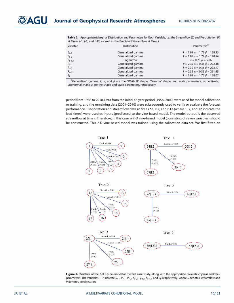
period from 1956 to 2010. Data from the initial 45 year period (1956–2000) were used for model calibrationor training, and the remaining data (2001–2010) were subsequently used to verify or evaluate the forecastperformance. Precipitation and streamflow data at times t-1, t-2, and t-12 (where 1, 2, and 12 indicate thelead times) were used as inputs (predictors) to the vine-based model. The model output is the observedstreamflow at time t. Therefore, in this case, a 7-D vine-based model (consisting of seven variables) shouldbe constructed. This 7-D vine-based model was trained using the calibration data set. We first fitted an

Figure 2. Structure of the 7-D C-vine model for the first case study, along with the appropriate bivariate copulas and theirparameters. The variables 1–7 indicate St-1, Pt-1, Pt-2, St-2, Pt-12, St-12, and St, respectively, where S denotes streamflow andP denotes precipitation.

Table 2. Appropriate Marginal Distribution and Parameters for Each Variable, i.e., the Streamflow (S) and Precipitation (P)at Times t-1, t-2, and t-12, as Well as the Predicted Streamflow at Time t

Variable Distribution Parametersa

St-1 Generalized gamma k = 1.09 α = 1.73 β = 128.33St-2 Generalized gamma k = 1.09 α = 1.72 β = 128.54St-12 Lognormal σ = 0.73 μ = 5.06Pt-1 Generalized gamma k = 2.32 α = 0.36 β = 292.38Pt-2 Generalized gamma k = 2.32 α = 0.36 β = 292.17Pt-12 Generalized gamma k = 2.35 α = 0.35 β = 291.45St Generalized gamma k = 1.09 α = 1.73 β = 128.07

aGeneralized gamma: k, α, and β are the “Weibull” shape, “Gamma” shape, and scale parameters, respectively;Lognormal: σ and μ are the shape and scale parameters, respectively.

Journal of Geophysical Research: Atmospheres 10.1002/2015JD023787

LIU ET AL. A MULTIVARIATE CONDITIONAL MODEL 10,121

appropriate marginal distribution to each variable by comparing the theoretical probability distributionsconsidered in this study based on their chi-square statistics (Table 1). The parameters of the appropriatedistribution chosen for each variable are given in Table 2. After obtaining well-fitted marginal distributions,a 7-D C-vine copula was used to join the margins and model the joint dependence structure. To establishthe C-vine model, the appropriate bivariate copula for each pair copula was determined using a methoddeveloped by Schepsmeier and Brechmann [2015] (i.e., the CDVineCopSelect function in the R package) asmentioned above. Figure 2 illustrates the appropriate bivariate copulas and their parameters for this 7-DC-vine model. Once the 7-D C-vine model had been established, the response variable (i.e., the predictedvariable), conditioned upon the explanatory variables (i.e., the predictors), was obtained using a 7-Dversion of equation (13). The forecasting performance of the 7-D C-vine model was tested using the valida-tion data set.

To appropriately assess the skill of the proposed vine-based model, we compared it with two popular data-driven models: ANFIS and SVR model. ANFIS combines the advantages of both ANNs and fuzzy systemswithin a single framework [Nourani et al., 2011]. A detailed description of ANFIS can be found in Jang[1993]. The appropriate ANFIS parameters (e.g., type and number of membership functions) are determinedby a trial-and-error method [Nourani et al., 2011]. SVR was proposed by Drucker et al. [1997] and is used todescribe regression with a support vector machine [Vapnik, 1995]. The basic idea of SVR is to compute a linearregression function in a high dimensional feature space, where the input data are mapped via a nonlinearfunction [Yu et al., 2006; Wei and Roan, 2012]. The SVR parameters were optimized using a two-step gridsearch method introduced by Yu et al. [2006] and Hsu et al. [2010]. The architectures and parameters ofANFIS and SVR used in this study are given in the supporting information.

The monthly streamflow forecasts (1 month ahead) during the validation period given by SVR, ANFIS, and theproposed vine-based model were compared in the form of a hydrograph, as illustrated in Figure 3. The 90%prediction uncertainty intervals generated from the vine-based model are also plotted. A visual comparisonindicates that the vine-based predictions are generally more consistent with the observations than those fromthe other data-drivenmodels. Additionally, this probabilistic forecasting is clearly more informative (e.g., in pro-

viding the prediction uncertainty) thanother deterministic models. Summarystatistics from the three models for 1month ahead forecasting over thevalidation period are given in Table 3.It is clear that the proposed model issuperior, to some extent, to SVR andANFIS in terms of R, NSE, and RMSE.

Figure 3. Time series plots of observed monthly streamflows and forecasts in the validation period using SVR, ANFIS, andthe vine-based model with 90% uncertainty prediction intervals for 1month ahead forecasting at Longchuan station.

Table 3. Summary Statistics of the SVR Model, ANFIS, and Vine-BasedModel for 1 Month Ahead Forecasting in the Validation Period atLongchuan Station

R NSE RMSE (m3/s)

SVR model 0.73 0.47 106.19ANFIS 0.72 0.51 102.04Vine-based model 0.76 0.53 99.44

Journal of Geophysical Research: Atmospheres 10.1002/2015JD023787

LIU ET AL. A MULTIVARIATE CONDITIONAL MODEL 10,122

3.2. Case Study 2: Improving Spatial Precipitation Estimation

We now describe the use of the proposed vine-based approach to improve spatial precipitation estimatesacross the Yangtze River basin. To refine the precipitation data derived from the tropical rainfall measuringmission (TRMM) precipitation data set (3B43 product), we used the observed precipitation records from 124meteorological gauges over the Yangtze River basin and simulated soil moisture data obtained from theadvanced microwave scanning radiometer-Earth-observing system (AMSE-E). The TRMM precipitation dataat 25 km spatial resolution were provided by the Goddard distributed active archive center (http://disc.sci.gsfc.nasa.gov/precipitation), and the 25 km spatial resolution AMSE-E soil moisture data set was down-loaded from the National Snow and Ice Data Center (http://nsidc.org/data/amsre/order_data.html).Observed precipitation data were provided by the National Climate Center of the China MeteorologicalAdministration (http://www.cma.gov.cn/). The location of the meteorological gauges is shown inFigure 4. As an illustration, we simply take the example of precipitation refinement for June 2010. We firstextracted the corresponding grid values from the TRMM precipitation data set and AMSE-E soil moisturedata set for June 2010 based on the location of meteorological gauges, using the extracting tool inArcGIS. This gave a 124-member ensemble of extracted TRMM precipitation, AMSE-E soil moisture, andobserved precipitation. This ensemble was split into two parts for the calibration and validation of theproposed algorithm. The first part includes 99 members (80%), with the remaining 25 members usedfor validation.

In this case, a 3-D vine-based model was used. Similar to the first case, the appropriate marginaldistribution for each variable was selected from the theoretical probability distributions considered inthe current study (Table 4). Table 5 gives the parameters of the chosen distributions. Figure 5

Figure 4. Location of precipitation gauges for both calibration and evaluation in the Yangtze River basin. The backgroundmap is the World Physical Map from ESRI (http://resources.arcgis.com/content/arcgisserver/10.0/gis-services).

Table 4. Statistics and P Value of the Chi-Square Test for Different Theoretical Distributions Fitted to Each Variable, i.e.,the TRMM Precipitation, AMSE-E Soil Moisture, and Observed Precipitationa

Distribution

TRMM Precipitation AMSE-E Soil Moisture Observed Precipitation

Chi-Square P Value Chi-Square P Value Chi-Square P Value

Normal 10.15 0.12 10.01 0.12 23.75 0.00Gamma 1.44 0.96 13.08 0.02 15.67 0.02Lognormal 6.18 0.40 11.17 0.08 9.88 0.13Weibull 3.29 0.77 6.62 0.36 10.45 0.11Generalized gamma 2.36 0.88 11.97 0.06 7.33 0.29

aThe best distribution for each variable is shown in bold.

Journal of Geophysical Research: Atmospheres 10.1002/2015JD023787

LIU ET AL. A MULTIVARIATE CONDITIONAL MODEL 10,123

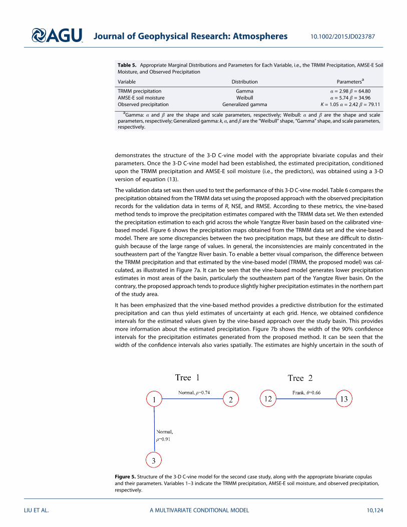
demonstrates the structure of the 3-D C-vine model with the appropriate bivariate copulas and theirparameters. Once the 3-D C-vine model had been established, the estimated precipitation, conditionedupon the TRMM precipitation and AMSE-E soil moisture (i.e., the predictors), was obtained using a 3-Dversion of equation (13).

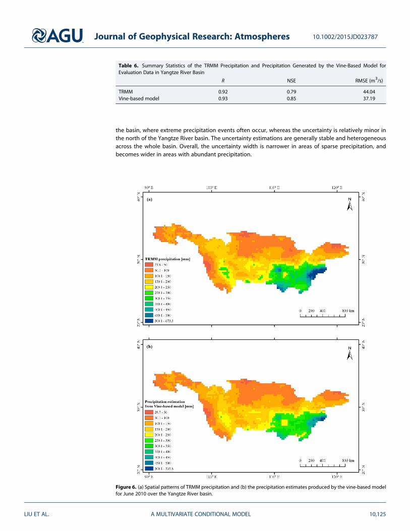
The validation data set was then used to test the performance of this 3-D C-vine model. Table 6 compares theprecipitation obtained from the TRMM data set using the proposed approach with the observed precipitationrecords for the validation data in terms of R, NSE, and RMSE. According to these metrics, the vine-basedmethod tends to improve the precipitation estimates compared with the TRMM data set. We then extendedthe precipitation estimation to each grid across the whole Yangtze River basin based on the calibrated vine-based model. Figure 6 shows the precipitation maps obtained from the TRMM data set and the vine-basedmodel. There are some discrepancies between the two precipitation maps, but these are difficult to distin-guish because of the large range of values. In general, the inconsistencies are mainly concentrated in thesoutheastern part of the Yangtze River basin. To enable a better visual comparison, the difference betweenthe TRMM precipitation and that estimated by the vine-based model (TRMM, the proposed model) was cal-culated, as illustrated in Figure 7a. It can be seen that the vine-based model generates lower precipitationestimates in most areas of the basin, particularly the southeastern part of the Yangtze River basin. On thecontrary, the proposed approach tends to produce slightly higher precipitation estimates in the northern partof the study area.

It has been emphasized that the vine-based method provides a predictive distribution for the estimatedprecipitation and can thus yield estimates of uncertainty at each grid. Hence, we obtained confidenceintervals for the estimated values given by the vine-based approach over the study basin. This providesmore information about the estimated precipitation. Figure 7b shows the width of the 90% confidenceintervals for the precipitation estimates generated from the proposed method. It can be seen that thewidth of the confidence intervals also varies spatially. The estimates are highly uncertain in the south of

Table 5. Appropriate Marginal Distributions and Parameters for Each Variable, i.e., the TRMM Precipitation, AMSE-E SoilMoisture, and Observed Precipitation

Variable Distribution Parametersa

TRMM precipitation Gamma α = 2.98 β = 64.80AMSE-E soil moisture Weibull α = 5.74 β = 34.96Observed precipitation Generalized gamma K = 1.05 α = 2.42 β = 79.11

aGamma: α and β are the shape and scale parameters, respectively; Weibull: α and β are the shape and scaleparameters, respectively; Generalized gamma: k, α, and β are the “Weibull” shape, “Gamma” shape, and scale parameters,respectively.

Figure 5. Structure of the 3-D C-vine model for the second case study, along with the appropriate bivariate copulasand their parameters. Variables 1–3 indicate the TRMM precipitation, AMSE-E soil moisture, and observed precipitation,respectively.

Journal of Geophysical Research: Atmospheres 10.1002/2015JD023787

LIU ET AL. A MULTIVARIATE CONDITIONAL MODEL 10,124

the basin, where extreme precipitation events often occur, whereas the uncertainty is relatively minor inthe north of the Yangtze River basin. The uncertainty estimations are generally stable and heterogeneousacross the whole basin. Overall, the uncertainty width is narrower in areas of sparse precipitation, andbecomes wider in areas with abundant precipitation.

Table 6. Summary Statistics of the TRMM Precipitation and Precipitation Generated by the Vine-Based Model forEvaluation Data in Yangtze River Basin

R NSE RMSE (m3/s)

TRMM 0.92 0.79 44.04Vine-based model 0.93 0.85 37.19

Figure 6. (a) Spatial patterns of TRMM precipitation and (b) the precipitation estimates produced by the vine-based modelfor June 2010 over the Yangtze River basin.

Journal of Geophysical Research: Atmospheres 10.1002/2015JD023787

LIU ET AL. A MULTIVARIATE CONDITIONAL MODEL 10,125

4. Discussion and Conclusions

In this study, we used the C-vine copula to model the joint dependence structure of multivariate data in theproposed vine-based model. The flexibility of the proposed model could be further enhanced by includingother vine copulas (e.g., the D-vine copula) to construct the joint dependence structure. A measure of thestatistical discrepancy among different vine copulas can be implemented to determine more appropriatevine structures for specific applications. This comparison could identify the similarities and differences inthe performance of various vine copulas and further relax the structure of the proposed model.

It should be emphasized that this method allows for predictions and estimations to be extended by includingmore additional conditioning variables. This means that higher dimensional forecasting models couldbe constructed based on the proposed method, in addition to the 3-D and 7-D cases illustrated in thecurrent study. One feasible approach is to decompose the original time series of potential predictors intoa number of periodic components (subseries) at different resolution levels via the wavelet transformation

Figure 7. (a) Difference between TRMM precipitation and estimates from the vine-based model for June 2010 over theYangtze River basin. (b) Spatial distribution of the 90% confidence intervals generated from the vine-based model.

Journal of Geophysical Research: Atmospheres 10.1002/2015JD023787

LIU ET AL. A MULTIVARIATE CONDITIONAL MODEL 10,126

[Tiwari and Chatterjee, 2010; Kisi and Cimen, 2011; Liu et al., 2014]. These periodic components could alsobe included in the proposed method as conditioning variables. In addition, for the case of streamflowprediction, climate indices such as the El Niño–Southern Oscillation (ENSO) could be considered as potentialpredictors. These are commonly used for predictions in data-driven models [e.g., Regonda et al., 2006; Kalraet al., 2013; Pokhrel et al., 2013]. It would also be very interesting to investigate the sensitivity of the overallperformance of the proposed model to the number of conditioning variables (potential predictors) andto explore whether specific conditioning variables provide any additional improvement in the accuracyof forecasts (or estimates). These issues are important components of future work with regard to furtherimprovement of the vine-based model.

In summary, we have presented a multivariate conditional model (i.e., the vine-based model) to produceprobabilistic forecasts or estimates for hydrometeorological variables. This model incorporates vine copulas,conditional bivariate copula simulations, and a copula-based conditional quantile function. The usefulnessand applicability of this model has been demonstrated via two different case studies. Our first case studyinvolves employing the vine-based model to generate 1month ahead streamflow forecasts incorporatingmultiple predictors. Our results show that the proposed model produces more reliable forecasts than othertraditional data-driven models such as SVR and ANFIS. Moreover, this probabilistic model allows the develop-ment of confidence intervals to assess the forecasting uncertainty. In the second case study, we refined pre-cipitation estimates from TRMM data set across a spatial region (Yangtze River basin) using the vine-basedmodel by constructing the joint dependence of the TRMM precipitation, AMSE-E soil moisture data, andobserved precipitation records from meteorological gauges. The validation results show that the proposedmodel successfully refines the spatial precipitation estimates. This model also provides additional informa-tion to account for the prediction uncertainty. Although the results are specific to the study basins used inthe experiments, the presented method has no restriction applied to different basins around the world. Itcould also be used for the prediction of hydrometeorological variables besides streamflow (e.g., temperature,wind speed, groundwater, and soil moisture).

Appendix A

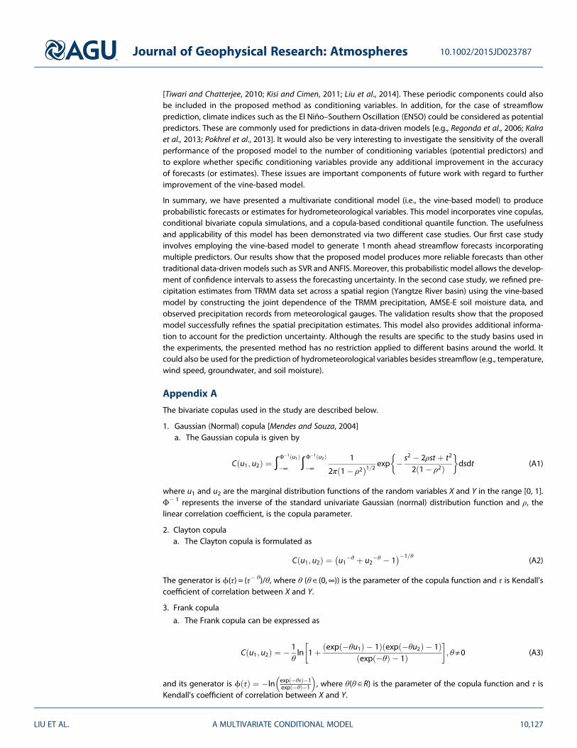
The bivariate copulas used in the study are described below.

1. Gaussian (Normal) copula [Mendes and Souza, 2004]a. The Gaussian copula is given by

C u1; u2ð Þ ¼ ∫Φ�1 u1ð Þ�∞ ∫

Φ�1 u2ð Þ�∞

1

2π 1� ρ2ð Þ1=2exp � s2 � 2ρst þ t2

2 1� ρ2ð Þ�

dsdt (A1)

where u1 and u2 are the marginal distribution functions of the random variables X and Y in the range [0, 1].Φ� 1 represents the inverse of the standard univariate Gaussian (normal) distribution function and ρ, thelinear correlation coefficient, is the copula parameter.

2. Clayton copulaa. The Clayton copula is formulated as

C u1; u2ð Þ ¼ u1�θ þ u2

�θ � 1� ��1=θ

(A2)

The generator is ϕ(τ) = (τ� θ)/θ, where θ (θ ∈ (0,∞)) is the parameter of the copula function and τ is Kendall’scoefficient of correlation between X and Y.

3. Frank copula

a. The Frank copula can be expressed as

C u1; u2ð Þ ¼ � 1θln 1þ exp �θu1ð Þ � 1Þðexp �θu2ð Þ � 1ð Þ

exp �θð Þ � 1ð Þ� �

; θ≠0 (A3)

and its generator is ϕ τð Þ ¼ �ln exp �θτð Þ�1exp �θð Þ�1

� �, where θ(θ ∈ R) is the parameter of the copula function and τ is

Kendall’s coefficient of correlation between X and Y.

Journal of Geophysical Research: Atmospheres 10.1002/2015JD023787

LIU ET AL. A MULTIVARIATE CONDITIONAL MODEL 10,127

ReferencesAas, K., C. Czado, A. Feigessi, and H. Bakken (2009), Pair-copula construction of multiple dependence, Insur. Math. Econ., 44(2), 182–198,

doi:10.1016/j.insmatheco.2007.02.001.Adamowski, J., H. Fung Chan, S. O. Prasher, B. Ozga-Zielinski, and A. Sliusarieva (2012), Comparison of multiple linear and nonlinear

regression, autoregressive integrated moving average, artificial neural network, and wavelet artificial neural network methods for urbanwater demand forecasting in Montreal, Canada, Water Resour. Res., 48, W01528, doi:10.1029/2010WR009945.

Bárdossy, A., and J. Li (2008), Geostatistical interpolation using copulas, Water Resour. Res., 44 W07412, doi:10.1029/2007WR006115.Bedford, T., and R. M. Cooke (2002), Vines–a new graphical model for dependent random variables, Ann. Stat., 30(4), 1031–1068, doi:10.1214/

aos/1031689016.Bennett, N. D., B. F. Croke, G. Guariso, J. H. Guillaume, S. H. Hamilton, A. J. Jakeman, S. Marsili-Libelli, L. T. Newham, J. P. Norton, and C. Perrin

(2013), Characterising performance of environmental models, Environ. Modell. Software, 40, 1–20, doi:10.1016/j.envsoft.2012.09.011.Brechmann, E. C., K. Hendrich, and C. Czado (2013), Conditional copula simulation for systemic risk stress testing, Insur. Math. Econ., 53(3),

722–732, doi:10.1016/j.insmatheco.2013.09.009.Cannon, A. J. (2008), Probabilistic multisite precipitation downscaling by an expanded Bernouilli-Gamma density network, J. Hydrometeorol.,

9, 1284–1300, doi:10.1175/2008JHM960.1.Chen, X., R. Koenker, and Z. Xiao (2009), Copula-based nonlinear quantile autoregression, Econ. J., 12, 50–67, doi:10.1111/j.1368-423X.2008.00274.x.Dawson, C. W., R. Abrahart, and L. See (2007), HydroTest: A web-based toolbox of evaluation metrics for the standardised assessment of

hydrological forecasts, Environ. Modell. Software, 22, 1034–1052, doi:10.1016/j.envsoft.2006.06.008.Drucker, H., C. J. C. Burges, L. Kaufman, A. Smola, and V. Vapnik (1997), Support vector regression machines, in Advances in Neural Information

Processing Systems, vol. 9, edited by M. Mozer et al., pp. 281–287, MIT Press, Cambridge, Mass.Fallah-Mehdipour, E., O. Bozorg Haddad, and M. A. Mariño (2012), Real-time operation of reservoir system by genetic programming, Water

Resour. Manage., 26(14), 4091–4103, doi:10.1007/s11269-012-0132-z.Fan, Y., and H. van den Dool (2004), Climate Prediction Center global monthly soil moisture data set at 0.5 resolution for 1948 to present,

J. Geophys. Res., 109, D10102, doi:10.1029/2003JD004345.Favre, A. C., S. El Adlouni, L. Perreault, N. Thiémonge, and B. Bobée (2004), Multivariate hydrological frequency analysis using copulas,Water

Resour. Res., 40, W01101, doi:10.1029/2003WR002456.Genest, C., and A. Favre (2007), Everything you always wanted to know about copula modeling but were afraid to ask, J. Hydrol. Eng., 12(4),

347–368, doi:10.1061/(ASCE)1084-0699(2007)12:4(347).Ghosh, S. (2010), SVM-PGSL coupled approach for statistical downscaling to predict rainfall from GCM output, J. Geophys. Res., 115, D22102,

doi:10.1029/2009JD013548.Hobæk Haff, I., A. Frigessi, and D. Maraun (2015), How well do regional climate models simulate the spatial dependence of precipitation? An

application of pair-copula constructions, J. Geophys. Res. Atmos., 120, 2624–2646, doi:10.1002/2014JD022748.Hsu, C. W., C. C. Chang, and C. J. Lin (2010), A practical guide to support vector classification. [Available at http://www.csie.ntu.edu.tw/~cjlin/

papers/guide/guide.pdf.]Huang, J., H. van den Dool, and K. P. Georgakakos (1996), Analysis of model-calculated soil moisture over the United States (1931–93) and

application to long-range temperature forecasts, J. Clim., 9(6), 1350–1362.Jang, J. S. R. (1993), ANFIS: Adaptive-network-based fuzzy inference system, IEEE Trans. Syst. Manage. Cybernetics, 23(3), 665–685,

doi:10.1109/21.256541.Joe, H. (1996), Families of m-variate distributions with given margins and m(m� 1)/2 dependence parameters, in Distributions With Fixed

Marginals and Related Topics, edited by L. Rüschendorf, B. Schweizer, and M. D. Taylor, pp. 120–141, Inst. Math. Stat., Hayward, Calif.Kalra, A., S. Ahmad, and A. Nayak (2013), Increasing streamflow forecast lead time for snowmelt driven catchment based on large scale

climate patterns, Adv. Water Res., 53, 150–162, doi:10.1016/j.advwatres.2012.11.003.Kao, S.-C., and R. S. Govindaraju (2007), A bivariate frequency analysis of extreme rainfall with implications for design, J. Geophys. Res., 112,

D13119, doi:10.1029/2007JD008522.Khedun, C. P., A. K. Mishra, V. P. Singh, and J. R. Giardino (2014), A copula-based precipitation forecasting model: Investigating the inter-

decadal modulation of ENSO’s impacts on monthly precipitation, Water Resour. Res., 50, 580–600, doi:10.1002/2013WR013763.Kim, G., and A. P. Barros (2001), Quantitative flood forecasting using multisensor data and neural networks, J. Hydrol., 246, 45–62,

doi:10.1016/S0022-1694(01)00353-5.Kisi, O., and M. Cimen (2011), A wavelet-support vector machine conjunction model for monthly streamflow forecasting, J. Hydrol., 399,

132–140, doi:10.1016/j.jhydrol.2010.12.041.Kurowicka, D. (2011), Introduction: dependence modeling, in Dependence Modeling, Vine Copula Handbook, pp. 1–17, World Scientific,

Singapore.Kurowicka, D., and R. Cooke (2006), Uncertainty Analysis with High Dimensional Dependence Modelling, Wiley, Chichester.Laux, P., S. Vogl, W. Qiu, H. R. Knoche, and H. Kunstmann (2011), Copula-based statistical refinement of precipitation in RCM simulations over

complex terrain, Hydrol. Earth Syst. Sci., 15, 2401–2419, doi:10.5194/hess-15-2401-2011.Li, C., V. P. Singh, and A. K. Mishra (2013a), A bivariate mixed distribution with a heavy-tailed component and its application to single-site

daily rainfall simulation, Water Resour. Res., 49, 767–789, doi:10.1002/wrcr.20063.Li, C., V. P. Singh, and A. K. Mishra (2013b), Monthly river flow simulation with a joint conditional density estimation network, Water Resour.

Res., 49, 3229–3242, doi:10.1002/wrcr.20146.Li, C., E. Sinha, D. E. Horton, N. S. Diffenbaugh, and A. M. Michalak (2014), Joint bias correction of temperature and precipitation in climate

model simulations, J. Geophys. Res. Atmos., 119, 13,153–13,162, doi:10.1002/2014JD022514.Liong, S., and C. Sivapragasam (2002), Flood stage forecasting with support vector machines, J. Am. Water Resour. Assoc., 38(1), 173–186,

doi:10.1111/j.1752-1688.2002.tb01544.x.Liu, Z., P. Zhou, G. Chen, and L. Guo (2014), Evaluating a coupled discrete wavelet transform and support vector regression for daily and

monthly streamflow forecasting, J. Hydrol., 519, 2822–2831, doi:10.1016/j.jhydrol.2014.06.050.Liu, Z., P. Zhou, and Y. Zhang (2015), A probabilistic wavelet-support vector regression model for streamflow forecasting with rainfall and

climate information input, J. Hydrometeorol., doi:10.1175/JHM-D-14-0210.1.Lopez-Paz, D., J. M. Hernandez-Lobato, and Z. Ghahramani (2013), Gaussian process vine copulas for multivariate dependence, in Proceedings of

The 30th International Conference on Machine Learning, edited by S. Dasgupta and D. McAllester, pp. 10–18, JMLR, Atlanta, Ga.Madadgar, S., and H. Moradkhani (2013), A Bayesian framework for probabilistic seasonal drought forecasting, J. Hydrometeorol., 14,

1685–1705, doi:10.1175/JHM-D-13-010.1.

Journal of Geophysical Research: Atmospheres 10.1002/2015JD023787

LIU ET AL. A MULTIVARIATE CONDITIONAL MODEL 10,128

AcknowledgmentsThis study was financially supported bythe key program of National NaturalScience Funds (4143000213), and theState Forestry Administration PublicBenefit Research Foundation of China(201204104). The data for this study areavailable for free at request from theauthor with the following e-mailaddress: zhiyong.liu@geog.uni-heidel-berg.de. We thank David Lopez-Paz andJosé Miguel Hernández-Lobato fortheir helpful suggestions whendeveloping the vine-based model. Wegratefully acknowledge the helpful andconstructive comments on themanuscript provided by the Editor andtwo anonymous reviewers.

Maity, R., M. Ramadas, and R. S. Govindaraju (2013), Identification of hydrologic drought triggers from hydroclimatic predictor variables,Water Resour. Res., 49, 4476–4492, doi:10.1002/wrcr.20346.

Mendes, B. V. M., and R. M. Souza (2004), Measuring financial risks with copulas, Int. Rev. Financ. Anal., 13(1), 27–45.McKerchar, A. I., and J. W. Delleur (1974), Application of seasonal parametric linear stochastic models tomonthly flow data,Water Resour. Res.,

10, 246–255, doi:10.1029/2004WR003562.Moradkhani, H., K. Hsu, H. V. Gupta, and S. Sorooshian (2004), Improved streamflow forecasting using self-organizing radial basis function

artificial neural networks, J. Hydrol., 295, 246–262, doi:10.1016/j.jhydrol.2004.03.027.Nash, J. E., and J. V. Shutcliff (1970), River flow forcasting through conceptual models, J. Hydrol., 10, 282–290, doi:10.1016/0022-1694(70)

90255-6.Nayak, P. C., K. P. Sudheer, D. M. Rangan, and K. S. Ramasastni (2005), Short-term flood forecasting with a neurofuzzy model, Water Resour.

Res., 41, W04004, doi:10.1029/2004WR003562.Nelsen, R. B. (2006), An Introduction to Copulas, Springer, New York.Noakes, D. J., A. I. McLeod, and K. W. Hipel (1985), Forecasting monthly riverflow time series, Int. J. Forecasting, 1, 179–190.Nourani, V., O. Kisi, and M. Komasi (2011), Two hybrid artificial intelligence approaches for modeling rainfall–runoff process, J. Hydrol.,

402(1–2), 41–59, doi:10.1016/j.jhydrol.2011.03.002.Nourani, V., A. Hosseini Baghanam, J. Adamowski, and O. Kisi (2014), Applications of hybrid Wavelet-Artificial Intelligence models in

hydrology: A review, J. Hydrol., 514, 358–377, doi:10.1016/j.jhydrol.2014.03.057.Pokhrel, P., Q. J. Wang, and D. E. Robertson (2013), The value of model averaging and dynamical climate model predictions for improving

statistical seasonal streamflow forecasts over Australia, Water Resour. Res., 49, 6671–6687, doi:10.1002/wrcr.20449.Regonda, S. K., B. Rajagopalan, M. Clark, and E. Zagona (2006), A multimodel ensemble forecast framework: Application to spring seasonal

flows in the Gunnison River Basin, Water Resour. Res., 42, W09404, doi:10.1029/2005WR004653.Ren, X., S. J. Li, C. Lv, and Z. Y. Zhang (2014), Sequential dependence modeling using Bayesian theory and D-vine copula and its application

on chemical process risk prediction, Ind. Eng. Chem. Res., 53(38), 14,788–14,801, doi:10.1021/ie501863u.Salvadori, G., and C. De Michele (2004), Frequency analysis via copulas: Theoretical aspects and applications to hydrological events, Water

Resour. Res., 40, W12511, doi:10.1029/2004WR003133.Sarangi, A., C. A. Madramootoo, P. Enright, S. O. Prahser, and R. M. Patel (2005), Performance evaluation of ANN and geomorphology-based

models for runoff and sediment yield prediction for a Canadian watershed, Curr. Sci., 89(12), 2022–2033.Schepsmeier, U., and E. C. Brechmann (2015), Package CDVine. [Available at http://CRAN.R-project.org/package=CDVine.]Serinaldi, F. (2009), A multisite daily rainfall generator driven by bivariate copula-based mixed distributions, J. Geophys. Res., 114 D10103,

doi:10.1029/2008JD011258.Sklar, A. (1959), Fonctions de Répartition à n Dimensions et Leurs Marges, Publ. Inst. Stat. Univ. Paris, 8, 229–231.Snedecor, G. W., and W. G. Cochran (1989), Statistical Methods, 8th ed., Iowa State Univ. Press, Iowa.Tiwari, M. K., and C. Chatterjee (2010), Development of an accurate and reliable hourly flood forecasting model using wavelet–bootstrap–

ANN (WBANN) hybrid approach, J. Hydrol., 1(394), 458–470, doi:10.1016/j.jhydrol.2010.10.001.Vapnik, V. (1995), The Nature of Statistical Learning Theory, Springer, New York.Wei, C., and J. Roan (2012), Retrievals for the rainfall rate over land using special sensor microwave imager data during tropical cyclones:

Comparisons of scattering index, regression, and support vector regression, J. Hydrometeorol., 13, 1567–1578, doi:10.1175/JHM-D-11-0118.1.Xu, Q., and T. Childs (2013), Evaluating forecast performances of the quantile autoregression models in the present global crisis in interna-

tional equity markets, Appl. Financ. Econ., 23(2), 105–117, doi:10.1080/09603107.2012.709601.Yu, P. S., S. T. Chen, and I. F. Chang (2006), Support vector regression for real-time flood stage forecasting, J. Hydrol., 328(3–4), 704–716,

doi:10.1016/j.jhydrol.2006.01.021.Zhang, L., and V. Singh (2006), Bivariate flood frequency analysis using the copula method, J. Hydrol. Eng., 11(2), 150–164, doi:10.1061/(ASCE)

1084-0699(2006)11:2(150).

Journal of Geophysical Research: Atmospheres 10.1002/2015JD023787

LIU ET AL. A MULTIVARIATE CONDITIONAL MODEL 10,129