FEDERAL RE:’EERVE OCTOBER

A Monetarist Model for EconomicStabilization: Review and UpdateKeith fri. Carison

SN APRtL 1970, Leonall Andersen arid t published anarticle, ‘‘A Monetarist Model for Econonuuic Stabiliza-tion,’’ in this Review.’ In this article, we developed asnuall model ofthe US. economy put’pot’tirig to exphairutim movements of certain key economic aggn-egates,ruamehy, nominal GNP, output (real GNPI, prices, inn-employnuent and short- and hong-term iruter’est rates.The model’s focus was on the i-ole of nuoruetary aggre-gates, in particular’, MI, in the detei’nuination of tlueseeconomic variables.

The purpose of the present article is to review thismodel in light of developments since 1970. This review

begins with a discussion of the development of theorginah model and is followed by an explanation ofthe key differences between it and the current version

of the model. This current version is analyzed bydemonstrating its response to shocks and its ability tosimulate, e,v post, movements of nominal GNP, output,prices, unemployment and interest rates.

01.11.1 .1,..1iE~

tn 1970, macroeconomic model-building was a pop-ulan’ exercise. The Michigan anti Wharton nuuodels,wluich had existed for a number of years, were corutin—uall being modified and updated.~’l’hue RIB—Ml’l’model, first publislued in 1968, was still being refined.’The Data Resources model was in thue developnuent

‘Andersen and Carlson (1970).2See Klein and Burmeister (1976), pp. 188—210 and Pp. 248—70.3de Leeuw and Gramlich (1968 and 1969).

stage.’ Each of these models contained a har’ge number’of equations and focused on a sector-al breakdown ofGNP derived from tlue Keynesian appr’oach to GNPdetermination.

Atudy and I felt thuat these models did not placeproper’ enuphasis otu flue r’ole of monetary actions.Furthernuore, they focused prinuarily on the short run

a pr-ojec’tion horizon of, at most, sever-al quarters.Ne wanted a nuodel that nioved fronu thie shor’t-r-un toa lorug—r-un dynanuic equihibr’iittuu with appropr-iate rec—ogmtion being given to initial conditiorus in this pro-cess. In addition, we wanted a model tluat was smallenough fluat the mter’relationships among the vari-ables could be understood easily. Moreover-, we

sought to build on existing research at tluis Bank,conubiruing various results to shed light on the issue ofecoruonuic stabilization flu a way that would overcoruuesome of the shortconuings of large—scale Keynesian—style models.

Our concer-ns about the state of model-buildirugstr-onghy influenced our efforts to develop aru altei-ria—tive macroeconomic model of the U.S. economy. Wewere iuot concer’rred about respecilving behavioral

equations (for exanuphe, consuruuptioru, iruvestnuetut,etc.(; r’ather’, we warned to capture empirical rela tionu—

sluips betweeru a i’elativelv few key nuacr’oeconom in:variables that wei-e inuuplic ithv gi’ouruder] in econtonuictheory.

‘hue furudaruuerutal hun ill ing block of our’ inonheh wasthe Aruden’seiu—Jor’daru t/-\—j( equation, which focused on

‘Klein and Burmeister (1976), PP. 211—31.

-.~ ~O3E~F B? / CA

the two chief artuus of policyruuaking, monetamy andfiscal actions? Althoughu tluis equation did not providea model of GNP determination, it was useful in fore-casting and in policy simulations. In the A-i equation,

c;NP was ‘‘deterruuined’’ solely by current arud pastmoruelar annl fiscal policy actions; other’ imufkrenceson GNt~wei’e found to tue n’andonu di.tnng the satuupheperinud investigated by Andersen—Jordan.

Atuother’ inuupor-tant buildirug block in tlue construc-tion of the Ander’sen—Cam-lson (A—C( ruuodel was theinterest rate equation, developed by Yohe amudKar-tuosky in 1969, in which interest rates wer~~systr~ni~—aticahhy relateni to past irutlation.’ Their- restilts wereconsistent with tlue Fisluerian tlueory of ituterest in thatthey showed that imuflation pr-enuia ar’e incorpoi’atedimutn) nonuinal iruter’est rates.

‘ro complete the tuuodeh, we needed equatiomus for

the unenuphoymnent i-ate and the price level. ‘rhe mostfanuous and genen-ally accepted unemploynuent rateequation, (Ieveloped by Arthuur Okun, was easily nuodi—

fled for’ our purposes.’ This equatioru combines a givenpotentiah GNP with actual GNP to provide aru estinuuate

of tlue unenuployruient rate.

Findirug aru appropr’iate price equation was a tuuon’echallenging task. Most latge models used a wage—ruuam’kup eqitatiotu and, mu sonue cases, some type ofPlulihips curve equatiomu. ‘l’luese equatiotus did nuot fultihhour n’eqtrin’enuuents. Instead, we developed a pn’ice mhIr~t—tion that cotuubinenl the Phillips curve m-esuhts withprice expectations? We used the coefficients otu thueinutlation ternus in the lomug—tem’muu inuterest rate equationuas our’ ruueasn.rre of price expectations. We tluouglut our’appn-oachu was novel and it seemed to work quitesatisfactor’ily at the timuue. Imu ret r’ospect, it seems rudi—nuentarv anuch luas ruot wot-ked as wehh iru recent veal’s.

7. 1771.71’ /777777 .7 7 . .~ *..i. .7J?J 7

The original model was i-ecum-sive, with tlue particu-lar form of eachu equation detem’nuuuued, for tlue nuost

pam’t, by tlue data. Since 1970, several charuges huavebeen ruuade in the n rode] iru terruus of I lue fom-nu of the

eqiratiorus amud the exogenous variables that areiruchuded.

‘l’lue original and cum-n’ent versions of the A—C nuonlehan-c summarized imu table 1. The model still has tluesante numluer of key endogenous vam-ialuhes; luowever,the thur’ee GNP variables — total spending, output atudprices — are now specified in rates of change instead

of fir’st differences. This change was made in the 1970s,when the fir-st-difference form luegan to exhituit heterti-skedasticity.” tn any event, the rate-of-change t’or-nu iseasier to inter’pret, amud the fundamental pm-operties ofthe model are unchanged. Monetary actions have ashom’t-run effect run output and a long—i-un effect on

p1-ices; fiscal actions have little effect on output or’

prices in either the short- or long-run.

Anotluer change was the addition of two nunun’e exog-enous var-iabhes — ener~’ pnces and exports. Thischange, necessitated by developments in tlue 1970s,was a ci-ude way to incorporate such complex fac-tors.” Nevertheless, it enabled us to keep the niodelsmall. Further-mor-e, changes in enen~’ pn’ices alsoenten- the current modeh through their influence onpotentiah GNP.

Annuther cluange, not shown explicitly in table 1, isthe redefinition of two exogenous variables — poteru-tial GNP and feden’ah expenditures. Potential GNP isnow estinuated using production—function nuethodsdeveloped by Rasche and ‘l’atom.” Feden’ah expendi-tures ar-c now cyclically adjusted rather than high—

employment.” The rationale underlying the fiscalmeasun’e remains the same — to construct a measureof federal spending that excludes the cyclical effect ofthe economy on the budget.

Finally, in the current version, the price, long-ter-nuinutei-est i-ate atud unemploynuent equatinurus are ad-justed fnur- autocor-r-elation tnu avoid biasirug the esti—mated standar-d errors of tlue coefficients.

Ahthoughu these charuges make it inupossibhe to com—pan-c meaningfully the sunumaty statistics for the twoversions, thue two versions show sinuilar estinuates ofthue impact of monetary and fiscal actions. An

eqiration—by—equatioru cornparrson is sutuunuarized intlue sluaded insert on page 21.

‘Carlson (1978).“Rasche and Tatom (1977b).“Rasche and Tatom (1977a).

“de Leeuw and Holloway (1983).

‘Andersen and Jordan (1968).

‘Yohe and Karnosky (1969).‘Okun (1962).‘See Considine (1969).

Table 1St. Louis Model: Original vs. Current Version

Original version Current versionSample period: I 1953-IV 1969 Sample period: 11960-tv 1984

(1) Total spending equation (1) Total spending equation

4 4 3~‘ 2.6/ m~M. ‘ :. e\i’~ V 308 12811.-’I U i i (I

4 3- cC extX‘0 io~m 5,57 >e 05 ~m cr6 ~e .07 ‘~ex 00

ft .66 SE 3.54 OW 1/5 H 32 3~ 391 UW 222

(2) Price equation (2) Price equation

5 3~P. 2.70 I ~ dO - 86 SPA, P 96 pe PE.‘0 rO

5. do - I 6BPA0

96Z2 - B0/3

~.d. 09 .pC 09 _d 05 p .01

H’ 87 S~ 1.0/ OW 141 A ~ S~ 148 nw 198

(3) Demand pressure identity (3) Demand pressure identity

D .xY. (XF X. 0 ~C IIIXI X r’ flroor

(4) Total spending identity (4) Total spending identity.Yr~ .~R’.\X t P.)t

(5) Long-term interest rate equation (5) Long-term interest rate equation

RL 1.28 06F~1 - 142/ 20RL 560 ::

16 16 Rx)t ‘ ~p(

o r U U. 4‘x 70 ~p 96 ~p 55 ~ 115 p. 16

R’ 92 SE 75 OW 69 Fl’ 07 SE 42 oW 1%

(6) Anhicipats price definition (6) Anticipated price definition1/

-WA v~,.~ ~ ~n01 I.- -) PA pR

Yp, 96 ~p .55

(7) Unemployment rate equation (7) Unemployment rate equation

U 3.90 - .040. ‘ 280 U Ui. 290 16UH .92 SE .30 OW 60 120

.71 SC 2? ~YW i 9~

(8) GNP gap identity (8) GNP gap identity

XI’ X XI- X0, xr G xr 100

rf~(~s~•Louis i%ilodel: Original vs. Current Versions

I hr lcrtal ~~‘‘~~‘g t’qrratiuri has1

u’r’ir c’liaurgi’d iritr’n’sl ‘alt’ equation is t’ssc’ntiallv LiIir’lhiiigc’cl.

‘noun a lust cifflc’rr’iir’r’ to rain’ ot—c’Ii,nnizc’ Ioi’jmn. arnri ‘ii’s-c’ its scrlr’ trnric’ticiri is to genir’r’atc’ tire t~c’tght’~oit

rUe cii rh.inigr’ ol r’\ports ,iflcI a chr’ninin tar’iahilt’. past prirr’s tcr risc’ in the rnvasun’ ot annliripatr’cl

rli’sigrrrd to c’apturc’ iii a II ode fl.a\ In’ ~r’hir’it_~’ shill pr’in’~.flit’ results or’ the r’,nrl~\c’rsiuIi li,id r’onsid—

,rttc’r’ luSt, hate hic’err ,iciric’ci. I hr I,iz~oil irimirir’~w,i’ r’i’,rl,It’ Lrfi})t’al Ipr’c’,ntnsr’ ~ji, VtiiS r’lcrsr’ Ic) tirir’ I

,rlsri slit,i’tc’iit’ci lit onu’ cjti;u’tc’i’ n’r’,iibt is not r,hsc’nc’rl iii Lint’ r’rir’r’eut \c’r’siorl. U-Iltririglr nit’ ttri’rii cii liii’ c’cjLizrticrnl is hoyt intuit

lii tIn’ c’tri’i’t’ril ~c’rs’riri. tlrt’ ~ri’ir-i’ r’cjtrzitnriri hi,us ,

sintijilen’ hr hI cr1 tint’ n’rlti,ttiori yt rich rric’ltncli’s artliner’ ,nclrlrliooah ~‘anahln’s nnicl Iicr~\ UI ratr’—ot

autcrr’nrn’n’r’hatncrri acIjrrsliirt~it. n’~‘‘‘‘It’ l~~ur’tic’ £4crocic’li;rnigc’ mmiii. itt r’r’’’\’ mItt’’, ,ll’r! rici’v rrtc’hricli’tl as Wi .

- . lit of tint’ urignnial instill trs rnislc’achnnn~ht’i’atisc’ therniclc’periclt’iit t’arnahmlr’. mini cIinrrnnirv tar’i~ihhr’src’Jmn’—

- r’(’Sl(IrliLls tt(’I’i’ itnL4ill\’ i’rii’n’c’latc’rl.sr’iitrrig price r’rmiitrub mci dt’c’orntnol no Ilir’ rarlt1970s arc’ alscr irir’lrjcic’ci, lit’ clr’nnnand p’~’ss~’~’tar i I hr sr’c mirnglv riraH’ c’hrLrlgc’ in the icmr’on cit r’cjLin

;rtile ‘eqti.itirirn ;i Ii;is i,r’c’ri i’c’clr’tirnr’tl tn at’ctiri iii”— tirmri 6 tvhic:hi clc1ioc’s aiitic’ipatn’cI iitlationi. insultsO,r4 rornniual ansi ‘c-al van’iaErlc’s l)c’nnn,inicl jnn’c’ssrrr’c’ is hiiron tin’ c:lntnngr- mmii lir~I dr.ltn’n’n’nc’i’ In r’atc’—cii—

nhc’tini’ci rncnt ,is actual ourllmtit gi’rnt lu n’c’lati\ n’ lo its change hrmi’rir. ‘lu’ r’rli’i’c’ilt ~‘r’i’siOul is mmcli i’asic’n’ 1cm

potential to c’sparrci. I lit’ r’oc’h’ljc’ic’ril on zjittic’i1hited interlmn’r’l. bring sirnnplv a vtn’ighlt’cl sum’ 01 mast rates

1u’ires. I us, non’ ;ilrliear’s cml cit inc yt ith Imotbi cr1 prire c’harigc’s

titt’nmi’n’tin’;il ;rnicl inst c’rrnpiu’nn’al c’—.tirni~rIi’s I tonet cr.— . . I mailt tlic’ uunc’irqmlnvonc’uit rqnuatinmun has

tthc’rn tis’ simm tori’ nit the Icing ter’nun motr’i’r’st ‘‘cjuia— ‘

- changed unIv shghtbv. I,ssentialiv. inc c’nrist,nnnt ‘iiis taken nun ac-count liii’ prrrdrrc’I ol the , ,

tlu’ nm-nina? t’ersicmri bias hc’en i’rqrlac’cti hv the bull—Inn c’oellic’renits ‘I GM am’. is iiioi’c’ Ut lOW yt illi “

c’nit1mlcit intuit ooc’nnphn rnmc’nl ‘air’, I his ratc’ is iii—

o’rtin’al c’’qmr’r’t.rticiil.tc’iitlc’ti to hit’ i’c,osnstent nun Ihc’ c’stinmatr’ oh Iiolc’ii—

uilikr’ time i’i’st ru tIn’ ecpnaticumis tint’ Icing’ tri’ni hal

Table 1 Continued -‘

Symbols.~ change in dollar values (note W X . tP. P and X outoul (CNP in 1958 pr ces in original mode? ard GNP ri

~X P .(X X ) r ‘982 prices in current modejannua rare of change n variab’e RE relative price of energy

V Iota? spending ~0NPin current prices) RL corporate Aaa bone rateM. money stock (Ml) U c,v,iian Lirierrployment rate

E. federal experidirti—es (high-employment in orIqirra’ rnodei G. GNP qap as a percent of potential outputand cycically ad

1usted in current modelr / dr.rnrnyvariahie(l 955 IV 1960 0 I 1961-lV 1969

LX. F. xports ot goods and services (fl carrr’rrt prices) Zi curriniy variable tI 1960-lV 1981 0 I 1982-lV 1984 1)P ONP deflator (1958 .00 in eriq;nal rnuc~’3l and ~p

1rrit.t’contmoidurmv fI 1960-Il 971 1119/3 IV 1984 0

1982 I 00 in cLirrent nlrudei) III 19/1 19/3U cerniand pressure 7.3 po~t-pncecoritro’ dummy tI 1960 I 973 II 1975-IV 1984

PA. anticipated price level 0.11 973-? 19Th iiXF potential output (council of Economic Advisers ebtimare in’

1958 prices in orginal mouei and Rascho I atom estimatein 1982 prices in current model)

Table 2The Current Model’s Response to a Fiscal Shock(shocked values denoted by prime)

Endogenous variablesQuarters Exogenous variable .. .......

elapsed E’E V “V X X p p u—u RL—RL

1 1.0454 1.0025 10022 1.0001 .061 0012 1 0440 1 0035 1 0027 1,0002 .107 .0043 1 0444 1 0032 1,0035 1.0005 137 .0094 10445 1.0030 1.0017 10008 .099 .0155 10457 1.0036 1 0028 I 0011 105 0206 1.0461 1.0036 1,0029 10014 125 0267 1,0454 1.0036 1 0025 1,0018 .116 0338 1.0455 1 .003o 1 0020 1,0022 .095 .038

12 1.0458 1 0036 1.0000 1.0033 004 05316 I 0479 1.0037 .9998 1.0041 020 05620 1 0467 1.0036 .9983 1 0047 067 05324 1 .0436 1.0034 9988 1 0050 049 04028 1,0424 1,0033 9977 1 0051 .082 02532 1.0391 1.0031 9984 1.0046 .067 .00336 1.0422 1 0032 .9990 1 0039 .046 .01540 1.0412 1.0032 1.0002 1 0033 008 .026

NOrE. To calculate percent change forE. V. X and P. subtract 1 and multiply by 100. U’--U and RL’-fl arc’ differences of percents

j)~f•p••q•/•p1.r~~ (Ji/ (:f ~ bLSC/iI ShOCk i:1Csi.O1s

The increase in cyclically adjusted expenditures

To demonstrate the properties of the current quickly influences total spending. The total effect,model, it was subjected to three different ‘shocks.” In however-, is at most a .37 percent increase or’ a mea-each case, the shock began in 1/1975, and the simu- sured elasticity of .08. The fiscal multiplier, ~Y/~E,lated response was calculated through IV/1984. The using average values for 1978—79 the middle of thethr’ee shocks are:’3 sample period), is .38. This is much lower’ than other

econometric models.’4

1. Fiscal shock-An increase in cyclically adjusted The dynamics of the model indicate that the initialexpenditures equal to 1 percent of GNP. increase in total spending is transmitted (jr-st and

temporarily to real GM’, then hilly to the price level. In

2. Monetary shock, A gradual increase in Ml over’ fact, it appears that the price level overshoots its finala year to 3 percent above the base path. equilibrium, implying an under-shooting of real GNP.

- Output and the price level continue to oscillate after

40 quarter’s, but the fiscal shock bias essentially no3. supply-side shock, A lower-ing of the world oil effect on output in the long run. Consequently, the

price by 20 percent. effect on the unemployment rate is small, with the

The results of simulating the model with each shock oscillation of the unemployment rate synchronousar-e shown in tables 2—4. These restrlts are summarized with output. Sirttilarly, the effect on the long—tem’min table s. interest rate is negligible even foun’ or five years after

the shock, as interest rates rise with inflation and fallwhen the rate of inflation declines.

‘2lhese are the shocks simulated for Protessor Klein’s model com~pamison seminar, which was reorganized in 1985. For results of theearlier seminar in the 1970s, see Klein and Burmeisrer (1976). ‘

4See Klein and Burmeister (1976), p. 338.

Table 3The Current Models Response to a Monetary Shock(shocked values denoted by prime)

Endogenous variablesQuarters Exogenous variableelapsed M M Y:V X.X P.P u-—u RL’—RL

1 1.0014 1.0004 1 0003 1.0000 .007 .0002 1.0073 1.0026 1,0019 1 0001 057 .0073 10188 1.0081 10084 1 0004 262 .0084 1.0280 1 0163 1 014b 1.0012 .532 0245 1.0300 1 0231 1 0208 1.0026 810 0516 1.0300 1.0265 1,0226 1.0045 961 086/ 1.0300 1.0272 1 0212 I 0067 .946 1258 1.0300 1 0272 1 0186 1.0090 851 .167

12 1 0300 1 0272 1 0087 1 0181 421 .30516 1.0300 1.0272 1 0016 1 0258 087 .39020 I 0300 1 0272 9948 I 0319 .202 41424 1 0300 1 0277 .9919 1 0361 .339 .37128 1,0300 1.0272 9891 1.0380 .450 2/232 1.0300 1 0272 9904 1.0370 402 14036 10300 1.0272 9930 1 0341 3’l 01440 1.0300 1 0272 9965 1.0311 164 076

NOTE: To calculate percent change for M. V X and P. subtract 1 and multiply by 100 U—U and RL A are differences ot percents

FEOERALRESERVEBM4KOFST. LOUtS OCTOBER1986

A monetary shock wor’ks thr’ough the model in the

same way the fiscal shock does — via total spending.The differ-ence is that the eflèct is much faster andlarger. Normally, a monetary shock is full)’ reflected in

total spending after four quarlers (see equation I intable I . With the exper-iment reported here, Ml buildsup over a yean”s time to 3 percent above the base path.Consequently, the frill effect on total spending is notregister’ed until the seventh quarter.

The dynamics of the model take over quite quicklywith respect to output and the p11cc level. Outputinitially rises, but after four’ yeans returns close to itsbase paLii level; it then falls below the base level as theinflation nate continues to increase, In fact, the elastic—

dv of the price level peaks at 1.27 alter seven year-s. ‘the40—qmrai’ten’ simulation is not long enough to detei-nrmethe nature of the long—run equibibr’ium.

‘the monetary shock produces a st r’ong oscillator)’movement in the unenip lovment rate. lrii tiallv, thisr’ate drops quick~v,falling to almost one per’ce ii (agepoint below its base path after only six quar-ters. After’four ‘ear-s, Li moves back to its base patti and then i

in creases above it, staving then-c br the remainder of

the sirnulation period.

‘l’he efl’ect of the monetary shock on interest de—pends directly on the pr’ice level r’esporise. Inflationand intet’est r-ates respond slowly to tile shock. As longas inflation increases, interest r’ates r’ise above theirbase path. When inflation slows after about sevenyear’s, inter-est n-aLes move back toward their base path.As wit Ii several other variables, the simulation periodis not long enough to deten’mine the nature of the finalequibibriu in.

‘to simulate the effect of a supply shock, the price ofoil per’ barr’el was assumed to dr’op 20 pen-cent, whichreduces the relative price of enen’gy by 8 pen-ceo t . Thisvar’iabte directly affects the pr-ice equation and mdi—

r’ectly affects the price level because the drop in theprice of oil is assumed to instantaneously incr-ease

potential output by .4 per-cetit . ‘~ liv assumption, totalspending is not affected by the supply shock, that is,the relative price of t-~nergvis riot included in the totalspendmg equation. This assumption is in dispute,however, as Tatom argues that total spending is tern’

porar’ilv affected by such a shock.’”

“Rasche and Tatom (June 1977).wTanom (1981). His argument rests on the signiticance of only one of

the lagged values of PE. For this reason, this variation has not beenintroduced into the version of the model summarized in table 1.

Table 4The Current Model’s Response to a Supply-Side Shock(shocked values denoted by prime)Quarters Exogenous variables Endogenous variableselapsed PE’/PE XE /XE VA’ X’/X P’/P tJ —u RL’—RL

1 9200 1 0040 1 0000 1.0000 9998 .109 0032 9200 1 0040 1 0000 .9999 .9996 172 0093 9200 1.0040 1 0000 1.0015 9992 .130 —.0164 .9200 1 0040 1 0000 1 0006 9988 .132 0235 .9200 10040 10000 10019 .9984 110 —0306 .9200 1 0040 1 0000 1 0026 9981 071 — 0357 9200 1 0040 1 0000 1 0030 9978 .049 0408 9200 1 0040 1 0000 1 0031 .9975 040 — 044

12 9200 1 0040 1 0000 1.0035 9963 .030 —.05816 9200 10040 1 0000 1 0049 9953 .025 06420 9200 1 0040 1 0000 1.0048 .9946 039 — 05924 9200 1 0040 1 0000 1 0061 9944 — 093 04328 .9200 1 0040 1 0000 1 0050 9946 .057 02232 9200 1 0040 1 0000 1 0050 .9948 044 — 00436 9200 10040 10000 10044 9953 018 .01140 .9200 1 0040 1 0000 1 0046 9957 — .029 019

NOTE To calculate percent change for PE. XF, V. X and P. subtract 1 and mubtnpfy by 100 U —U and AL’ A are dnfferences of percents

Table 5Estimated Elasticities for the Current Model

With respect to With respect to With respect to

Quarterselapsed

fiscal shock (E) monetary shock (M) supply shock (PE)

V X P V X P V X P

1 .06 .05 .00 .29 .21 .00 .00 - .00 .002 .08 .06 .00 .36 .26 .01 .00 .00 .013 .07 .08 .01 .43 .45 .02 .00 - .02 .014 .07 .04 .02 .58 .52 .04 .00 — .01 .028 .08 .04 .05 .91 .62 .30 .00 — .04 .03

12 .08 .00 .07 .91 .29 .60 .00 -.04 .0516 .08 — .00 .09 .91 .05 .86 .00 — .06 .0620 .08 — .04 .10 .91 —.17 1.06 .00 — .06 .0724 .08 —.03 .11 .91 — .27 1.20 .00 — .08 .0728 .08 —.05 .12 .91 -.36 1.27 .00 -.06 .0732 .08 —.04 .12 .91 -32 1.23 .00 -.06 .0736 .08 —.02 .09 .91 —.23 1.14 .00 —.06 .0640 .08 .00 .08 .91 — .12 1.04 .00 - .06 .05

Tables 4 and 5 show that output and prices r’es pond snnal I. In fact, the elasticities (calculated with respectquite slowly to this shock, Mon’eover’, the maximum to the relative price ofenergvt ane sirnilai’ in magnitudeeffect, whic,h occun’s after about six year’s, is r’elat ively to those for Ibder’al expendi to r’es.

OCIOEE’R

Chart

Nominal GNP

if

To provide some indication of model performance,the model was simulated e~post during several peri-

ods aftcc 1969. Denoting such simulations as ex postmeans that all simulations were within the samplepen’iod and the exogenous variables took on theiractual values. All simulations were dynamic; that is,

once the simulation was started, the model generatedits own lagged values.

These simulations are summarized in char’ts 1—3

and table 6. Unfortunately, these results mean little bythemselves because then’e is no basis for’ comparison.Results for’ similar simulation exercises with other

models have been published for the l960s and ear’ly1970s, but are not readily available for mon-c recent

periods. Consequently, any conclusions aboutmodel’s performance are impressionistic.

if,,if1”,,,,,,i’,_-,, i•ifif••~if’if•i•”

Charts 1—3 show the results of simtnlating’c’. ~ and1~for the fitll simulation per’iot final 1970 thn’ough 1984.Since the total spending equation contains no endog-

enous variables, the model simulation shown in chart1 simply shows the fit of that equation. That fit obvi-ously does quite poorly on a quarter~to~quan’ten’basisbut seems to follow the contours over seven-al quarters,

almost as if a moving aver-age had been applied to theactual obsewations. A desirable featun’e of this equa—tion is that the quar’ter—to—quar-ten’ er’r’ors (10 riot tend tocumulate over time. ‘l’he errors in the estimated equa—tion an’e nob correlated.

Table 6 shows that the RMSE of Y incn’eases over

the

Percent compounded Annual Rate at Change30

Percent

30

25

20

Is

10

5

1970 11 12 73 74 75 71, 17 73 79 80 81 82 33 1934

0

-s

OF S1 LOUIS. OCTOBSO 1955

chort 2

Real GNP

time and, even when standardized by the level of GN P(SRM SE I, it continues to grow as the sinnulation period

moves toward the present. This suggests that therelationship between ~‘ and NI has become looser’recently.

OLIIIJLI.1 (r’ss lb

The relative degree of sticcess in siniulating totalspending is carried over’ to the simulation ol output.

The model simulated A well over the 1,jr~r’iods,althoughit under-estimated economic strength during the ex-

pansion from the 1973—7.5 recession. The other per’iodof substantial difference has occurred since the tl urd

quan-ter of 1983. ‘tile model indicated a recession,

which did not occinn-.

When the model is simulated over different periods,no consistent patter-n emerges lbr the SRMSE for X. Inthe 1970—84 period, the SRMSE for X exceeded that forY. In the 1975—84 and 1979—84 periods, however, the

SRMSE for X was less than for Y, apparently reflectingthe emen’ging importance of aggregate demand shocksrelative to supply-side shocks during these pet-iods.

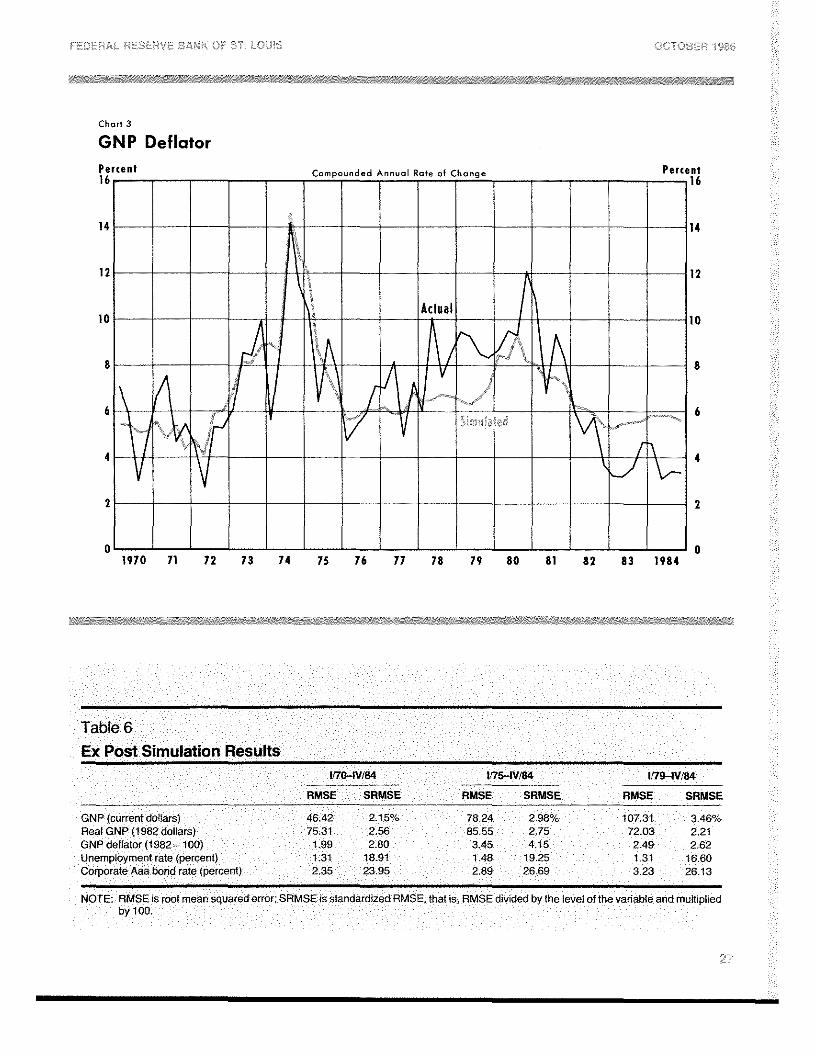
The resinits of simulating the inflation r’ate over the1970—84 period are shown in chan-t 3. Generally speak-ing, the niovemen ts were approximated cloning the1970—77 pen-iod, but the accelen-atiori starting in thesecond quarter of 1978 was not picked up until a yearor so later. The essence of the general decelerationfrom mid—1980 was captured, but since mid—1982. themodel has overestimated inflation by about 2 percent-age points.

These visual impressions are borne out in the calcu-lation of RMSE for the CNP deflator. The shortest andlatest period was best with a standar-dized 1-IMSE of2.62 percent. The 1975—84 period was the wor-st withan SRMSE of 4.15 percent. ‘liw simulation for the

Percent Compounded Annual Rate of change16

Percent16

12

8

4

0

-4

1970 71 72 73 74 75 76 71 18 79 80 81 82 83 1984

-8

-12

FEOEIRA•L RESERVE 66496 OF St LO-UL~

Chort 3

OOTOSER 1968

GNP DeflatorPercent

16

14

12

10

8

6

4

2

082 83 1984

Table 6Ex Post Simulation Results

1/70-IV/84 Ills-IW84 h179-IV/84

RMSE SRMSE AMSE SRMSE RMSE SRMSE

GNP (current dollars) 4642 2 15% 78 24 2.98% 10731 3 46%Real GNP (1982 dollars) 7531 2.56 8555 275 7203 2.21GNP deflator (1982 100) 1 99 280 3.45 4 15 249 2.62Unemployment rate (percent) 1 31 1891 1 48 1925 1.31 1660Corporate Aaa bond rate (percent) 2 35 23.95 2.89 2669 3 23 26 13

Percent16

14

12

10

8

6

4

2

01970 11 72 13 14 75 76 77 18 19 80 81

NOTE RMSE s root mean squared error, SAMSE is standardized AMSE that is, AMS divided by the level of the variable and multipliedby 100.

FEDERAL RESERVE BANK OF ST. OCTOBER 1986

overall period was in between, with an SRMSE of 2.79

percent.

fl:IflIJilni’fl661fl1 and .tnfrrtlSl .•ffiFs

Table 6 shows that the l-tMSE for’ simulations of thecivilian u nem ploynient nate and tile Aaa bond rate donot vary by much over differ-ent simulation per’iods.‘l’he RMSE is more meaningful for these comparisonsthan SRMSE because the RMSE is already expressed inpercentage points.

Simr.nlations of the nnovements of the Aaa bond i-atewere gener-ally utlimpressive. Although the RMSE waslittle different for the alternative simulation per’iods, itincreased as the siniulat ion was br-ought closer to thepresenit.

The St. Louis model, as originally published in Apr-il

1970, was designed to focus on the importance ofmonetary actions in the determination of spending,output and prices. its structure differed substantiallyfronr other econometric models at that time. It con—sisted of the Anden’sen—Jor-dan GNP equation and sev-en-al oIlier’ empin-ical relationships; it was n’ecirrsive inform. It estimated GNP directly using nnorietar’v andfiscal variables, in sharp contrast to the conventionalapproach of estimating the components of GNP and

then summing them to obtain a GM’ estimate,

Since 1970, the gener-al form of the model has been

maintained, but seven-al changes in its specificationand estimation have been made. One notable changehas been simplification ~- using rates of change in-stead of first differences. Another is the addition ofsupply—side variables ~- the relative pr-ices of energyand price control and decontrol cItnmmies and, most

r-ecently, a d nmmv in the GN P equation to rap tur’e theshift in the relationish p since 1981. Other changesincluded alternative estimates of potential output andfederal expenditures, and adjustments for’ atrtocorne—lab ion in several of the equations.

Despite these changes, the proper’ties of the nnodelren rain essentially unchanged. NI oneta rv act ions havea large short—n-un effect on total spending, oin tput andinnempl oynnent ; oven’ the long ru ri, however’, the effecton total spending is alnnost entirely r-eflected in the

price level, with very little effect on output atid unem-ployment. l”iscal actions have small short—run effectsthat disappear in terms of outputl quite quickly.While the supply—side effects are not strong accor-ding

to conventional elasticities, these effects can be impor—tarit if ener~/prices move dr’amaticallv.

The per-fortnance of the model is difficinlt to gauge,but, for the most part, the sinnr.n lation r’estilts weredeemed successful. Ex post simulations are the con—ventional method of assessitig a models performance,hut they ar’e more meaningful when conrpai-ed withthose fnoni othen- models. I’her-e have been no pub-lished studies of 110w othen’ models are per4or’rning inthe I980s, A more accurate evaluation awaits compar-i—

son with similar results from other current models.

6L416611)1’TH c11~.sAndersen, Leonalt C., and Keith M. Carlson. ‘A Monetarist Model

for Economic Stabilization,” this Review (April1970), pp. 7—25.

Andersen, Leonatt C., and Jerry L. Jordan. “Monetary and FiscalActions: A Test of Their Relative Importance in Economic Stabili-zation,” this Review (November 1968), pp. 11—24.

Carlson, Keith M. ‘Does the St. Louis Equation Now Believe inFiscal Policy?” this Review (February 1978), pp.13—19.

Considine, William. “Public Policy and the Current Inflation,” pre-pared as part ot a summer intern program at the U.S. TreasuryDepartment (September 5, 1969).

de Leeuw, Frank, and Edward Gramlich. “The Channels of Mone-tary Policy,” Federal Reserve Bulletin (June 1969), pp. 472—91.

________ “The Federal Reserve-MIT Econometric Model,” Fed-eral Reserve Bulletin (January 1968), pp. 11—46.

de Leeuw, Frank, and Thomas M. Holloway. “Cyclical Adjustmentof the Federal Budget and Federal Debt,’ Survey of Current Busi-ness (December 1983), pp. 25—40.

Klein, Lawrence A., and Edwin Burmeister, eds, Econometric ModelPerformance (University of Pennsylvania Press, 1976).

Okun, Arthur M. “Potential GNP: Its Measurement and Signifi-cance,” 1962 Proceedings ofthe Business and Economic StatisticsSection of the American Statistical Association, pp. 98—104.

Rasche, Robert H., and John A. Tatom. “Energy Resources andPotential GNP,” this Review (June 1977a), pp.10—24.

________ “The Effects of the New Energy Regime on EconomicCapacity, Production, and Prices,” this Review (May 1977b), pp.2—12.

Tatom, John A. “Energy Prices and Short-Run Economic Perfor-mance,” this Review (January 1981), pp. 3-17.

Yohe, William P., and Denis S. Karnosky. ‘Interest Rates and PriceLevel Changes, 1952—69,” this Review (December 1969), pp. 18—38.