a molecular dynamics derived finite element method for...
TRANSCRIPT
A Molecular Dynamics derived Finite Element Method for Structural Simulations andFailure of Graphene Nanocomposites
A. A. R. Wilmes 1, S. T. Pinho2
1 Department of Aeronautics, Imperial College London ([email protected])
2 Department of Aeronautics, Imperial College London ([email protected])
Abstract. The recent rise of 2D materials, such as graphene, has expanded the interest innano-electromechanical systems (NEMS). The increasing ability of synthesizing more exoticNEMS architectures, creates a growing need for a cost-effective, yet accurate nano-scalesimulation method. Established methodologies like Molecular Dynamics (MD) trail behindsynthesis capabilities because the computational effort scales quadratically. The equilibriumequations of MD are equivalent with those of the computationally more favourable FiniteElement Method (FEM). However, current implementations exploiting this equivalence re-main limited due to the FEM iterative solvers requiring a large number of lengthy force fieldderivatives and specifically tailored element topologies. This paper proposes a formal deriva-tion of the merged Molecular Dynamic Finite Element Method (MDFEM) which establishesan uncoupling of the force field potentials from the element topologies. An implementationapproach, which does not require manual derivations, is presented. Different non-linear MDforce field potentials are implemented exactly within the FEM, at reduced computational costs.The proposed multi-scale and multi-physics compatible MDFEM is equivalent to to the MDas demonstrated by an example of brittle fracture in Carbon Nanotubes (CNT).
Keywords: MDFEM, FEM, AFEM, Molecular, Fracture.
1. INTRODUCTION
Simulating the mechanical response of nano-structures is important for a wide andrapidly increasing range of areas. Continuous progress in nano-synthesis capabilities, togetherwith graphene’s first applications in nano-electromechanical systems (NEMS) [1–3], havefurther spurred interest in efficient, robust and flexible numerical nano-simulation methods.
One of the main challenges for nano-simulation models consists of achieving a suitablebalance between the accuracy of the physical representation and the scale of applicability. Atone extreme, Ab Initio simulations, based on Density Functional Theory (DFT), can offer highaccuracy but cannot readily be used for domains beyond O(102) atoms. At the other extreme,classical Molecular Mechanics (MM) and Dynamics (MD) methods [4–6] only resolve nucleimotion (Born-Oppenheimer approximation), but may be typically applied to domains with
Blucher Mechanical Engineering ProceedingsMay 2014, vol. 1 , num. 1www.proceedings.blucher.com.br/evento/10wccm

O(109) atoms [7]. Parallel supercomputing simulations have succeeded in increasing thisnumber to O(1012) atoms [8]. A variety of intermediate theory levels have emerged such asthe hybrid DFT-MD Car-Parrinello method [9], or the reactive MD force fields [10, 11].
The MD method has increasingly been incorporated in the Finite Element Method(FEM) framework [12–23] as the equilibrium equations of MD and FEM may be expressed inequivalent forms. The resulting Atomistic Finite Element Method (AFEM) [13], also referredto as Molecular Dynamic Finite Element Method (MDFEM) [24], is both computationallymore favourable than MD [25], and offers a significant increase in compatibility and inte-grability with larger scale continuum FEM simulations. Structural mechanics elements (e.g.trusses, beams) have been used to analyse the overall mechanical behaviour of nano-scaleentities, such as carbon nanotubes (CNT) [26–28], as well as the deformation of individualbonds [12, 14].
MDFEM is mostly applied to carbon nano-structures due to the maturity of carbon-specific force fields and the large interest in graphene, CNTs, and other fullerene derivedcompounds. However, non-carbon applications have been reported for other nano-structures,such as particulate metal matrix nano-composites [22] or boron-nitride nanotubes [23].
Several comprehensive presentations and reviews of AFEM/MDFEM and its imple-mentations are available [24, 25, 29, 30]. Nonetheless, MDFEM remains a non-consolidatedmethod because formal derivations are scarce, with significant differences arising on thetopologies of the required MDEFM-specific elements. The available MDFEM element de-signs vary considerably in complexity and their implementation is often not straight-forward[16,21,25]. Additionally, only few proposed MDFEM element topologies are fully non-linearand non-local capable. This has lead to MDFEM often being implement using readily avail-able, standard structural FEM elements such as beams, trusses and springs [12,14,20,31,32].However, the use of structural elements results in the following detrimental restrictions ofMDFEM’s full non-linear capabilities:
1. Inadequate Element Topologies with Limited Non-Local CapabilitiesSevere inconsistencies arise where non-local force fields are approximated with struc-tural elements which are topologically not adequate to represent multi-body potentialsinvolving three or more atoms. Alternatively, structural FEM elements, often featuringrotational degrees of freedom (DoF), are used although the definition of point angles foratoms is highly ambiguous.
2. Limited Large Deformation Analysis CapabilitiesThe mechanical behaviour of structural elements is inherently different from that ofatomic bonds, especially for large-deformation analyses. An attractive alternative isthe use of non-linear springs to represent the potentials accurately for large strains.However, torsional springs for instance, require rotational DoF to be included in themodel upon which they can act and they are unable to represent, for example, cross-deformation sub-potentials such as stretch-bend interactions.

3. Inability to Perform Conformational AnalysesStructural FEM elements typically prevent MDFEM from being able to perform theoften required relaxation or conformational analysis step prior to the load application.This is due to the FEM elements’ default inability to incorporate knowledge of thenatural bond characteristics (e.g. bond length, angles), which are, in all but the simplestgeometries (e.g. planar graphene), different from the overall structure’s equilibriumpositions.
This paper presents a fully non-linear MDFEM model, based on appropriate MDFEM-specificelement topologies. A formal derivation of the MDFEM equilibrium equations, from firstprinciples, is presented in section 2. The formulation can accommodate any type of MD forcefield, from classical, non-reactive many-body and pair-wise potentials, to advanced adaptivereactive bond order force fields (section 3). The presented derivation intrinsically considersall geometric non-linear effects and is explicitly independent of ambiguous rotational DoF.
The equilibrium equation for the smallest, fully non-linear MDFEM element topology,which can represent the molecular force field potential or each of its constituent sub-potentials,is derived exactly in section 4.2, together with exact expressions for the required correspond-ing Hessians (tangent stiffnesses). The element topology designs, presented in section 4.3, areintentionally kept as small and comprehensive as possible.
Analogously to the separation, in FEM, between the element topologies and the mate-rial properties, section 4.5 demonstrates how this MDFEM formulation uncouples the molec-ular force field from the element topologies. Significant advantages for the implementationand the stability analysis of the presented MDFEM arise from this uncoupling approach (4.6)— most notably, the ability to differentiate between instabilities in the system due to the forcefield or chemical bond failure (constitutive instability) and those due to the geometry of thestructure (geometrical instability).
A method for the straight-forward implementation of the relevant equations (sections2, 4.2 and 4.5) with the given element topologies is described in sections 5.1 and 5.2. A briefoverview of optimization techniques for the equations’ numerical implementation is given insection 5.3.
The model is shown to identically reproduce MD predictions [33] of brittle fracturein CNT with defects (section 6.1). Additionally, conformational analyses of complex three-dimensional Pillared Graphene Structures (PGS) are presented in section 6.2. Conclusionsabout this MDFEM implementation are given in section 7.

2. EQUATIONS OF EQUILIRBRIUM
2.1. Hamilton’s Principle and Lagrange’s Equation
A variational statement of equilibrium for a discrete domain can formally be derivedfrom Hamilton’s principle, which subjected to a Legendre transform, leads to Lagrange’sequation. For a non-relativistic analysis, the domain’s kinetic energy, T , equals its kinetic co-energy, T ∗, so that the dynamic equilibrium within a conservative potential field, V , withoutdamping effects, may hence be stated as:
d
dt
(∂ (T (q))
∂q
)T
+
(∂ (V (q))
∂q
)T
=d
dt(∇q (T (q))) +∇q (V (q)) = g, (1)
where the vector derivatives adhere to the numerator layout convention. The domain’s n
displacements, given in generalized coordinates, are denoted by q ∈ Rn×1 and are definedrelative to an unloaded equilibrium position q0 = 0, while g ∈ Rn×1 represents the corre-sponding generalized forces. The operator ∇v represents the gradient of a scalar function withrespect to the vector v, in the same dimensions as v, i.e. ∇v = ∂/∂vT = (∂/∂v)T. Moreover, qis chosen such that the kinetic energy, T , may be explicitly dependent only on the generalizedvelocities, q ∈ Rn×1, i.e. T = T (q).
2.2. From Lagrange’s Equation to a discrete Finite Element Method
The translational displacements of all atoms in a global Cartesian coordinate system,u ∈ Rn×1, constitutes a natural choice of q for a discrete particle domain. Hence, the gen-eralized corresponding forces, denoted f ∈ Rn×1, are a set of linear forces only. RotationalDoF with corresponding moments are inappropriate quantities as atoms represent point parti-cles. Using the choice q = u, equation (1) becomes:
d
dt(∇u (T (u))) +∇u (V (u)) = f . (2)
The rest state of the atomic domain, when u = u0 = 0, is fully defined by the equilibriumpositions of all n/3 atoms, denoted by x ∈ Rn×1. Any deformed state of the domain mayhence be described by r = x+ u, see figure 1.
Figure 1. Coordinate System and Displacements Definitions for Atoms i and j
In the framework of Newtonian mechanics, the kinetic energy, T , for a domain consti-tuted of point masses as defined in figure 1, can be expressed as:
T (u) =1
2uTMu, (3)
where the mass matrix, M, is diagonal. Equation (2) may hence be expressed as:
Mu+∇u (V (u)) = f , (4)
where ∇u (V (u)) is the transpose of the potential’s Jacobian relative the the domain’s dis-placements, i.e.∇u (V (u)) =
(JVu
)T, such that global equilibrium, equation (4), may beequivalently expressed as:
Mu+(JVu
)T= f . (5)
Equation (5) is typical for a Finite Element Method framework and can be solved using aNewton-Raphson scheme provided the Hessian of the potential, expressed as:
HVu =
∂ (∇u (V (x,u)))
∂u, (6)
can be determined.
3. MOLECULAR FORCE FIELDS
3.1. Constituent Sub-Potentials
In general, a molecular force field, V , consists of the superposition of sub-potentials,VS , as:
V (c) =∑S
VS (cS) , (7)
where S represents the set of included sub-potentials, c ∈ Rm×1 represents the m charac-teristic variables (e.g. bond lengths and angles) and cS ∈ RmS×1 denotes the mS specificcharacteristic variables required for evaluating the sub-potential VS .
In general, classical force fields include sub-potentials for specific deformation modessuch as bond stretching, bending and torsion, while more elaborate force fields may featureadditional sub-potentials for mixed-mode deformations such as stretch-stretch, stretch-bend orbend-bend interactions [6]. Both non-reactive force fields and reactive bond-order force fieldsmay be expressed in the form of equation (7). The many-body coupling bond-order variable,which is required in reactive fields (usually denoted b or B [10, 11]), may be also interpretedas a characteristic variable. Classical MD sub-potentials (e.g. stretch, bend, torsion) tend

to depend on a single characteristic variable only, mS = 1, while cross-deformation sub-potentials (e.g. stretch-bend) may depend on two or more variables, mS > 1. The non-reactiveLobo-Keating (fullerene-specific) force field for instance, may be stated as [34]:
VLobo-Keating = VS + VB + VI
=1
2
n/3∑i=1
3∑j=1
α
4r20
(rij · rij − r20
)2+
n/3∑i=1
2∑j=1
3∑k=j+1
β
r20
(rij · rik +
1
2r20
)2
+ (8)
+
n/3∑i=1
γ (di · di) , (9)
where VS, VB and VI refer to the stretch, bend and inversion sub-potentials respectively. Thevector from atom i to atom j in the deformed state is denoted rij = rj − ri. The naturalbond length is given as r0, and di represents the dangling vector, which is defined as di =
ri1 + ri2 + ri3. The force field’s fitting parameters are α, β and γ. As another example, theMM3 (general-purpose) force field may be expressed as [6]:
VMM3 = VS + VB + VT + VSB + VTS + VTB + VBB + VVDW, (10)
where VT, VSB, VTS, VTB, VBB and VVDW refer to the sub-potential energies of the torsion,stretch-bend, torsion-stretch, torsion-bend, bend-bend and Van der Waals interactions respec-tively. The reader is referred to [6] for the detailed sub-potential expressions.
A particularly interesting reactive force field is the Brenner potential [10, 11], whichis of the form:
V =
n/3∑i=1
n/3∑j>i
[VR (rij)− BijVA (rij)
], (11)
where VR and VA represent the repulsive and attractive atomic interactions. The bond order,Bij , is a highly non-linear function of the bond angles centred at atoms i and j, the coordi-nation number of atoms i and j as well as the coordination numbers of the first and secondneighbour atoms to i and j.
3.2. Characteristic Variables
The force field’s characteristic variables, c, may always be expressed in the form c =
c (x,u), so that it is possible to reformulate the potential explicitly as:
V (c (x,u)) =∑S
VS (cS (x,u)) =∑S
VS (x,u) . (12)

(a) Bond Stretching (b) Bond Bending (c) Bond Torsion
Figure 2. Characteristic Variables of Force Field Potentials
Figure 2 outlines a selection of common characteristic variables used by a variety of forcefields. For instance, rij and θijk in figure 2 are respectively given by:
rij = ∥rj − ri∥ = ∥xj + uj − xi − ui∥, (13)
θijk = arccos
(rji · rjkrijrjk
)= arccos
((xi + ui − xj − uj) · (xk + uk − xj − uj)
∥xi + ui − xj − uj∥∥xk + uk − xj − uj∥
). (14)
A vast literature giving variable-defining sketches, such as in figure 2, is available and thereader is referred to [35] for a comprehensive collection.
4. MOLECULAR DYNAMIC FINITE ELEMENT METHOD
4.1. Introduction
In some cases, force field potentials may be represented exactly or approximatelyby FEM structural elements. However, the use of structural elements leads to significantrestrictions, as outlined in section 1. In any case, it is possible to deduce a non-linear accuraterepresentation of equation (5) within FEM through defining individual elements for each sub-potential as outlined in this section.
4.2. Constituent Sub-Hessian Matrices
Taking advantage of the sub-potential nature of force fields, equation (7), the totaldomain’s Jacobian, JV
u in equation (5), and Hessian, HVu in equation (6), can be obtained as:
JVu (x,u) =
∂V (x,u)
∂u=∑S
∂VS (x,u)
∂u=∑S
JVSu (x,u) . (15)
HVu (x,u) =
∂ (∇u (V (x,u)))
∂u=∑S
∂ (∇u (VS (x,u)))
∂u=∑S
HVSu (x,u) . (16)
Equations (15) and (16) show how the total potential, V , Jacobian, JVu , and Hessian, HV
u ,of the overall domain, Ω, may be divided into superimposed sub-domains, ΩS , as shown infigure 3. It follows naturally that an element topology may be created for each individual

sub-potential, VS (cS (x,u)), which is able to supply the necessary characteristic variablescS (x,u). These element types are then superposed when meshing the atomic domain. Thespacial superposition of multiple element types outlines a first fundamental difference be-tween the proposed MDFEM and the classical FEM, as in the latter, element superpositioningin the same location is atypical.
Figure 3. Illustration of Domain Decomposition and Sub-Domain Partitioning
For each sub-potential, VS , the corresponding sub-domain, ΩS , may in turn be dividedinto pS partitions (figure 3), where V i
S ≡ VS in partition i and is zero elsewhere. In general thepartitioning pattern varies for different sub-potential domains, ΩS (i.e. some sub-potentials re-quire information from more atoms than others, see figure 4). It follows that the sub-potentialmay be then expressed as the summation over the partitions:
VS (x,u) =
pS∑i
V iS
(xiS,u
iS
), (17)
where xiS ∈ RnS×1 and ui
S ∈ RnS×1 are the nS components of x and u respectively which arenecessary for evaluating V i
S . Equation (17) indicates that pS number of elements are neededfor each sub-potential and that these elements must include the necessary atoms to supply xi
S
and uiS . It follows that HVS
u and JVSu may be obtained by first evaluating:
JV iS
uiS
(xiS,u
iS
)=
∂V (xiS,u
iS)
∂uiS
and HV iS
uiS
(xiS,u
iS
)=
∂(∇ui
S(V i
S (xiS,u
iS)))
∂uiS
, (18)
followed by an assembling of equations (18) of the type:
JVSu (x,u) = ⊔VS
pS
(JV iS
uiS
(xiS,u
iS
))and HVS
u (x,u) = ⊔VSpS
(H
V iS
uiS
(xiS,u
iS
)), (19)
where ⊔VSpS
denotes the assembly operator which assembles the contributions of all pS Jaco-
bians, JV iS
uiS(xi
S,uiS) ∈ R1×nS , into the corresponding positions within JVS
u (x,u) ∈ R1×n and
similarly the contributions of of all pS Hessians, HV iS
uiS(xi
S,uiS) ∈ RnS×nS , into HVS
u (x,u) ∈Rn×n.

The numerical solution to the global equilibrium problem, equation (5), using an iter-ative solution scheme requiring the Hessian (equation (6)), can therefore be obtained triviallyusing equations (18) and (19) together with suitable element topologies.
4.3. Element Topologies
The topology of the elements required for each sub-potential is determined by therespective components of cS . The most compact and comprehensive element designs arehence identical to the characteristic variable-defining sketches for each force field (fig. 2).Figure 4 features a set of basic element shapes used for non-reactive and reactive force fields.Elements for reactive force fields include more atoms as the bond-order characteristic has ahigher non-locality.
(a) NR-2 (b) NR-3 (c) NR-4-C (d) NR-4-S (e) R-6
Figure 4. Selection of Non-Reactive (NR) and Reactive (R) Element Topologies
Table 1 outlines a small selection of characteristic variables which the elements infigure 4 can supply and which sub-potentials they may be required for.
Table 1. Element Topologies, Characteristic Variables, cS , and Applicable Sub-Potentials, VS .NR-2 NR-3 NR-4-C NR-4-S
r12 =√r12 · r12 r21 =
√r21 · r21 cos (ϕ1234) = −r123 · r234 d21 = d1 · d1
r212 = r12 · r12 (r21r23 cos (θ123)) = r21 · r23 r123 =
(r12 × r23r12r23
)d1 =
√d1 · d1
VS, VVDW VB, VSB, VSS VT, VTS, VTB VI, VIT, VBBS = Stretch, B = Bend, T = Torsion, I = Inflexion, IT = Improper Torsion, SS = Stretch-Stretch
SB = Stretch-Bend, BB = Bend-Bend, TS = Torsion-Stretch, TB = Torsion-Bend, VDW = Van der Waals
Reactive element topologies require at least six atoms (e.g. R-6), three on each sideof the bond [10, 11], while as many as fourteen may be required in case that coordinationnumbers above three are considered. In general, larger elements share characteristic variableswith smaller element, so that they could represent the smaller element’s sub-potential as well.However, this approach is to be discouraged because larger element topologies cannot bemeshed as close to the domain boundary as smaller topologies, leading to increased edgeeffects. Finally, it can be noted that since the characteristic variables are defined in a globalframe of reference (FoR), these elements do not require a local to global reference frametransformation prior to assembly.
4.4. Derivation of the Element Jacobian and Hessian
Implementing the elements of section 4.3 within the Finite Element Method requiresderiving each element’s contribution to the global equilibrium equations, equation (5), i.e JV i
S
uiS,
as well as deriving HV iS
uiS, which is required for the iterative solution scheme. Modern inter-
preted processing languages are increasingly capable of rapid symbolic derivation of analyti-cal expressions so that the Jacobian and Hessian may be generated symbolically. This processfor an element type, omitting the i and S indices for clarity of notation, may be representedby:
VS (c) ,x,u, c (x,u) → Symbolic Processor →HVS
u ,JVSu
. (20)
The computational effort for this process is small; however, the resulting expression for asingle entry of the Hessian,
(HVS
uS
)i,j
, can become prohibitively long for the implementation ina compilable language (e.g. the FORTRAN 90/95 standard has a maximum of 5148 charactersper statement, although specific compilers may offer higher limits). These excessively longderivatives easily occur for higher-order sub-potentials requiring elements with nS > 6, orwhere cS requires more complex functions such as inverse trigonometric relations.
More aggravatingly, the direct evaluation of JV iS
uiS
and HV iS
uiS
compounds the elementtopology information with that of the implemented force field. Force field characteristics andelement topology properties may be kept uncoupled, section 4.5, resulting in a significantlyincreased flexibility of this MDFEM formulation in combining different element types fordifferent potentials.
4.5. Decoupling Element Topology and Force Field
Noting equation (12), each entry in the sub-potential’s Jacobian and Hessian tensors,(JVSu
)i,j
and(HVS
u
)i,j
in equation (18), may equivalently be expressed as:
(JVSu
)1,i
=∂VS
∂ui
=
mS∑k=1
∂VS
∂ck
∂ck∂ui
=
mS∑k=1
(JVSc
)1,k
(Jcu)k,i , (21)
(HVS
u
)i,j
=∂2VS
∂ui∂uj
=
mS∑k=1
∂ck∂ui
(mS∑l=1
∂2VS
∂ck∂cl
∂cl∂uj
)+
mS∑k=1
∂VS
∂ck
∂2ck∂ui∂uj
=
mS∑k=1
(Jcu)k,i
(mS∑l=1
(HVS
c
)k,l
(Jcu)l,j
)+
mS∑k=1
(JVSc
)1,k
(Hcu)k,i,j , (22)
where JVSc ∈ R1×mS and HVS
c ∈ RmS×mS are the sub-potential’s respective Jacobian andHessian tensors relative to the characteristic variables. Similarly, Jc
u ∈ RmS×nS and Hcu ∈
RmS×nS×nS are the Jacobian and Hessian tensors of the characteristic variables relative to theelement nodal DoF. The process in equation (20) may thus be restated as:
VS (c) ,x,u, c (x,u) → Symbolic Processor →JVSc ,HVS
c ,Jcu,H
cu
, (23)
which may then be used to directly generate the compilable language script as:
JVSc ,HVS
c ,Jcu,H
cu,Eq. (21)-(22)
→ Interpreted Language →
→HVS
u , JVSu , in a compilable language
. (24)
4.6. Stability and Implementation Advantages of Uncoupling Force Fields and ElementTopologies
Equations (21) and (22), hereafter termed reconstruction equations, result in the fol-lowing advantages:
1. Reduced Complexity of DerivativesThe reconstruction equations require the symbolic evaluation of more, yet shorter deriva-tives so that the latter may be more comfortably implemented in a compilable languagescript. Additionally, the computational effort for the iterative solver reduces becauseless operations are required to evaluate HVS
u and JVSu by using the reconstruction equa-
tions than by a direct approach.
2. Separation of Force Field Potentials from Element TopologiesThe force field sub-potentials become completely uncoupled from the element types sothat a library of pre-compiled derivatives for both the force fields on one hand, and theelements on the other hand, can be developed and stored separately.
3. Independent Scaling of Derivatives’ LengthThe above uncoupling also results in entries of JVS
c ,HVSc , Jc
u and Hcu to scale in length
only with either the complexity of VS (c) or c (x,u) respectively, but any compoundeffect is avoided. The only condition for selecting an element type for a sub-potential isthat the element must be able to supply all characteristic variables required by VS .
4. Independent Analysis of Constitutive and Geometrical InstabilitiesFinally, and perhaps most importantly, the reconstruction equations allow for an analy-sis of the two structural instabilities which may occur during MDFEM simulations. Thefirst is a geometrical instability, which occurs for instance during buckling. The secondis a chemical-constitutive instability, which can arise if the force field’s potential fea-tures an inflexion point. In this case, the Hessian tensor (tangent stiffness) will cease tobe positive-definite and negative eigenvalues may appear in the solution procedure.
A guaranteed identification of a constitutive instability cannot be achieved by consid-ering HVS
u directly. In general, an MDFEM element is geometrically under-determined

in some directions of global space, so that the latter’s geometrical under-determinationmasks the chemical bond yielding in the overall Hessian, HVS
u .
However, constitutive instabilities can readily be detected by testing for positive-definitenessof HVS
c . An expensive eigenvalue analysis to test for the positive-definite nature of HVSc
can be avoided by recognizing that it is a Hermitian matrix and thus Sylvester’s criterionmay be applied.
5. IMPLEMENTATION
5.1. Numerical Implementation of Global Equilibrium
The presented formulation was implemented symbolically in MATLAB [36], and theresultant formulations were exported in a FORTRAN format, which is suitable for the FEpackage ABAQUS [37]. The latter allows for the definition of customized element types,termed User Elements, with freely definable element topologies and constitutive properties.A FORTRAN subroutine (UEL), which takes the nodal variables (x,u) as input, must sup-ply the elements’ Jacobian, JVS
u , and Hessian, HVSu , to the FEM solver. A flowchart of the
overall implementation including pre-processing (e.g. symbolic derivations, atom seeding,element meshing) is presented in section 5.2, while section 5.3 covers additional optimizationperformed on the generated subroutine using Common Subexpression Elimination (CSE).
5.2. Preprocessing
Figure 5. Implementation Pre-Processor and Solver
A symbolic pre-processor (fig. 5) generates all required files for implementing thecurrent MDFEM within the FEM. The user input file must define the choice of force fieldand element topologies, the atomic geometry and the boundary conditions (BC); additionaladvanced options, such as periodic boundary conditions or optimization techniques are avail-able.
The requested geometry is seeded and meshed with all required element types beforethe element types’ Jacobians, JVS
c (x,u), Jcu (x,u), and Hessians, HVS
c (x,u), Hcu (x,u), are
derived symbolically. The latter are translated into FORTRAN language, CSE optimized andthen combined with the reconstruction equations (21) and (22) in the UEL subroutine script.
The Element Library contains the characteristic variable definitions, c = c (x,u),and node connectivities of each element type. The force field library contains the force fielddefinitions in the form V (c) =
∑S VS (c). Hence, the implementation of a new force field
constitutes no additional time cost once an Element Library has been established.

5.3. Script-Level Local, Common Subexpression Elimination (CSE)
The characteristic variables’ vectorized definitions, equations (13) and (14), result inexpressions for the entries of the characteristic variables’ Jacobian, Jc
u, and Hessian, Hcu,
which are ideally suited for local CSE optimization. While many compilers include CSEcapability, it was chosen to implement CSE at the FORTRAN script level, especially becauseelaborate characteristic variables may still cause prohibitively long statement expressions (e.g.NR-4’s cos (ϕijkl) = −rijk · rjkl). In general, using a pre-computed temporary variable t0 =
t0 (x,u), an entry of the Hessian, Hcu, may be reformulated as:
(Hcu)i,j,k = h (x,u) = h0 (x,u, t0) , (25)
where t0 is chosen so as to maximize the length reduction of h (x,u). Subsequent temporaryvariables may use preceding temporary variables: tl = tl (x,u, t1, . . . , tl−1) for l > 1, suchthat after l substitutions, the Hessian is evaluated as (Hc
u)i,j,k = hl (x,u, t0, . . . , tl). Thetemporary variables may be reused immediately after this evaluation, in order to keep theregister allocation low. For the MM3 force field, this CSE results in an overall 80% reductionof mathematical operations, while the overall script length generally reduces by 73%.
6. APPLICATIONS
Two applications of the implemented MDFEM are presented. Firstly, the equivalenceof MDFEM and MD is demonstrated using a static, non-linear fracture simulation of CNT.Secondly, non-equilibrium meshes of complex three-dimensional Pillared Graphene Struc-tures (PGS) are allowed to relax, hence demonstrating the current implementation’s capabilityto perform conformational analyses.
6.1. Brittle Failure of Carbon Nanotubes (CNT) with Defects
The MD study by Belytschko et al. [33], investigating the effects of defects on the frac-ture behaviour of CNT, was chosen as a reference to demonstrate the equivalence of MDFEMand MD in a highly non-linear environment up to, and including bond failure. Three CNTconfigurations [33] (table 2) were tested in a static analysis, u = 0, and were strained axiallyto fracture. The effect of defects was included by softening a bond in the middle of the CNTby 10% (i.e. effectively a 0.9 multiplication factor was applied to both JVS
u and HVSu of the
affected elements). Failure of a bond is detected in the current MDFEM implementation bytesting each bond’s HVS
c for positive-definiteness, as discussed in section 4.6. Following Be-lytschko et al. [33], the Brenner potential [10], equation (11), is approximated in this exampleby a Morse type potential of the form:
V = VS + VB = α[
1− e−β(rij−r0)]2 − 1
+
1
2γ (θijk − θ0)
2 [1 + λ (θijk − θ0)4] . (26)
The above potential was developed to be equivalent to the Brenner force field for strains up
to 10% [33], but without suffering from the subsequent camel-back problem in the force-displacement relation. The fitting constants for equation (26) are: r0 = 1.39 A, θ0 =
2.094 rad, α = 6.03105 nN A, β = 2.625 A−1, γ = 9.0 nN A/rad2 and λ = 0.754 rad−4 [33].The present formulation identifies CNT uniquely by a triplet of integers, such as (20, 0, 10).The first two indices, (20, 0), refers to the commonly-used integer notations for the chiralvector, Ch = 20 · a1 + 0 · a2, where a1 and a1 denote the graphene lattice vectors. Thethird index, 10, identifies the CNT height as 10 · ∥T∥, where T is the orthogonal translationalvector [17, 38].
Table 2. Model Specifications - Brittle CNT Failure SimulationsCNT
Configuration Atoms VS Element pS VB Element pBEquilibrium
Length l0(A)
(12,12,20) 984 NR-2 1452 NR-3 2855 48.151(16,8,10) 1128 NR-2 1664 NR-3 3279 53.588(20,0,10) 820 NR-2 1200 NR-3 2359 41.700
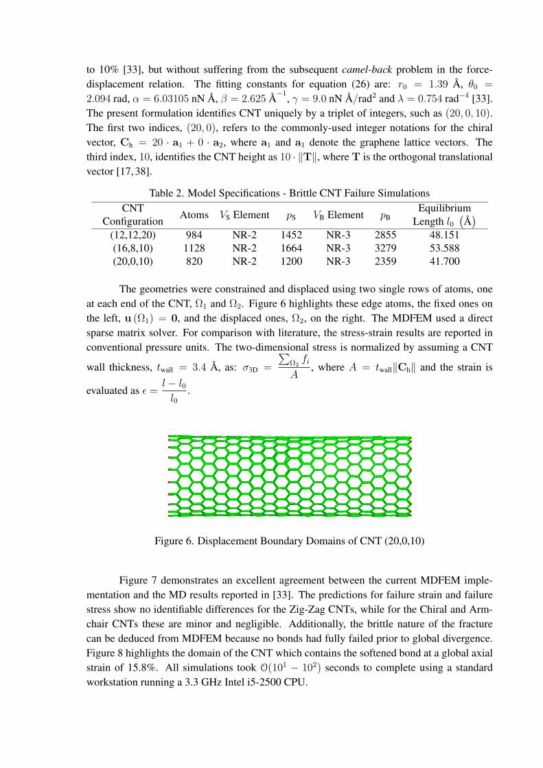
The geometries were constrained and displaced using two single rows of atoms, oneat each end of the CNT, Ω1 and Ω2. Figure 6 highlights these edge atoms, the fixed ones onthe left, u (Ω1) = 0, and the displaced ones, Ω2, on the right. The MDFEM used a directsparse matrix solver. For comparison with literature, the stress-strain results are reported inconventional pressure units. The two-dimensional stress is normalized by assuming a CNT
wall thickness, twall = 3.4 A, as: σ3D =
∑Ω2
fi
A, where A = twall∥Ch∥ and the strain is
evaluated as ϵ =l − l0l0
.
Figure 6. Displacement Boundary Domains of CNT (20,0,10)
Figure 7 demonstrates an excellent agreement between the current MDFEM imple-mentation and the MD results reported in [33]. The predictions for failure strain and failurestress show no identifiable differences for the Zig-Zag CNTs, while for the Chiral and Arm-chair CNTs these are minor and negligible. Additionally, the brittle nature of the fracturecan be deduced from MDFEM because no bonds had fully failed prior to global divergence.Figure 8 highlights the domain of the CNT which contains the softened bond at a global axialstrain of 15.8%. All simulations took O(101 − 102) seconds to complete using a standardworkstation running a 3.3 GHz Intel i5-2500 CPU.
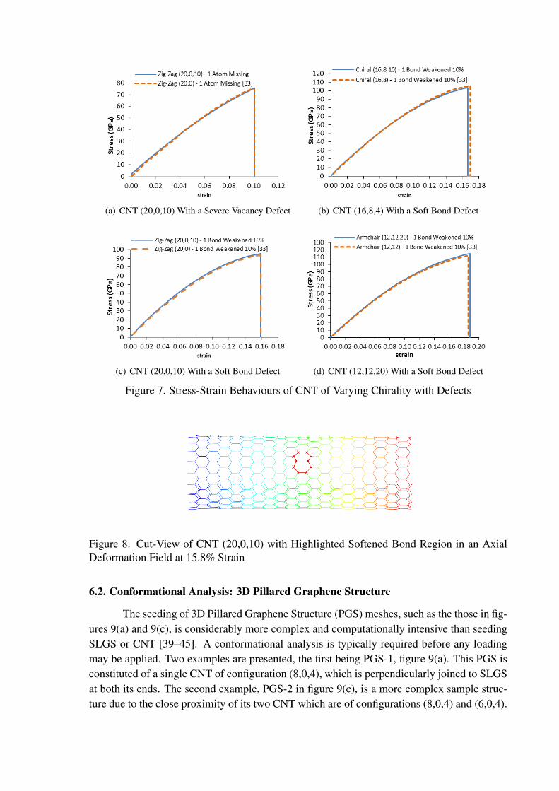
(a) CNT (20,0,10) With a Severe Vacancy Defect (b) CNT (16,8,4) With a Soft Bond Defect
(c) CNT (20,0,10) With a Soft Bond Defect (d) CNT (12,12,20) With a Soft Bond Defect
Figure 7. Stress-Strain Behaviours of CNT of Varying Chirality with Defects
Figure 8. Cut-View of CNT (20,0,10) with Highlighted Softened Bond Region in an AxialDeformation Field at 15.8% Strain
6.2. Conformational Analysis: 3D Pillared Graphene Structure
The seeding of 3D Pillared Graphene Structure (PGS) meshes, such as the those in fig-ures 9(a) and 9(c), is considerably more complex and computationally intensive than seedingSLGS or CNT [39–45]. A conformational analysis is typically required before any loadingmay be applied. Two examples are presented, the first being PGS-1, figure 9(a). This PGS isconstituted of a single CNT of configuration (8,0,4), which is perpendicularly joined to SLGSat both its ends. The second example, PGS-2 in figure 9(c), is a more complex sample struc-ture due to the close proximity of its two CNT which are of configurations (8,0,4) and (6,0,4).
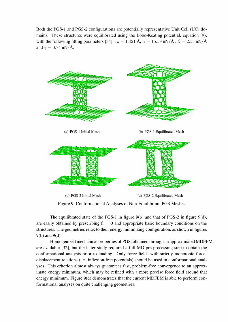
Both the PGS-1 and PGS-2 configurations are potentially representative Unit Cell (UC) do-mains. These structures were equilibrated using the Lobo-Keating potential, equation (9),with the following fitting parameters [34]: r0 = 1.421 A, α = 15.59 nN/A , β = 2.55 nN/Aand γ = 0.74 nN/A.
(a) PGS-1 Initial Mesh (b) PGS-1 Equilibrated Mesh
(c) PGS-2 Initial Mesh (d) PGS-2 Equilibrated Mesh
Figure 9. Conformational Analyses of Non-Equilibrium PGS Meshes
The equilibrated state of the PGS-1 in figure 9(b) and that of PGS-2 in figure 9(d),are easily obtained by prescribing f = 0 and appropriate basic boundary conditions on thestructures. The geometries relax to their energy minimizing configuration, as shown in figures9(b) and 9(d).
Homogenized mechanical properties of PGS, obtained through an approximated MDFEM,are available [32], but the latter study required a full MD pre-processing step to obtain theconformational analysis prior to loading. Only force fields with strictly monotonic force-displacement relations (i.e. inflexion-free potentials) should be used in conformational anal-yses. This criterion almost always guarantees fast, problem-free convergence to an approx-imate energy minimum, which may be refined with a more precise force field around thatenergy minimum. Figure 9(d) demonstrates that the current MDFEM is able to perform con-formational analyses on quite challenging geometries.
7. CONCLUSION
A mathematically rigorous, fully non-linear derivation and a comprehensive imple-mentation of the Molecular Dynamic Finite Element Method (MDFEM) has been presented.The model has shown to yield numerical predictions identical to MD fracture simulations andhas produced, to the best of the authors’ knowledge, novel results by achieving the first fullyMD-equivalent conformational analyses performed within MDFEM.
The formulation bases itself on the simplest possible MDFEM element topologieswhich are available throughout literature, and hence the force field characteristic variables aredefined unambiguously. This intuitive and clear approach significantly facilitates the numeri-cal implementation of MDFEM and should spark an increased use of the latter.
Moreover, the present MDFEM derivation uncouples the force field potentials fromthe element topologies in a way which is analogous to the separation of constitutive rela-tions and element topologies in classical FEM. This approach further enhances the flexibility,clarity and accessibility of the present formulation. Solely the force field in its basic form,V = V (c), and the definitions of the characteristic variables, c = c (r,u), are required asinputs to model the chosen MD force field exactly within MDFEM. Additionally, the forcefield vs. element topology uncoupling results in the current model’s ability to differentiateexplicitly between geometrical instabilities (e.g. buckling) and constitutive instabilities (e.g.bond failures) during the simulations.
Finally, the current model is ideally suited for multi-scale integration (hierarchicaland concurrent) with larger-scale FEM simulations. The given derivation of MDFEM mayequally well accommodate multi-physics effects if the element topologies are enriched withappropriate degrees of freedom beyond the current displacement DoF.
Acknowledgements
The present project is supported by the National Research Fund, Luxembourg (1360982)
Roshan Bhalla is acknowledged for generating the PGS meshes.
8. REFERENCES
[1] K. S. Novoselov, A. K. Geim, S. V. Morozov, D. Jiang, Y. Zhang, S. V. Dubonos, I. V.Grigorieva, and A. A. Firsov, “Electric field effect in atomically thin carbon films,” Sci-ence, 306, 666–669, 2004.
[2] C. Chen, S. Rosenblatt, K. Bolotin, P. Kim, I. Kymissis, H. Stormer, T. Heinz, andJ. Hone, “Nems applications of graphene,” in Electron Devices Meeting (IEDM), 2009IEEE International, 1 –4, dec. 2009.
[3] R. A. Barton, J. Parpia, and H. G. Craighead, “Fabrication and performance of graphenenanoelectromechanical systems,” Journal of Vacuum Science & Technology B: Micro-electronics and Nanometer Structures, 29, 050801, 2011.
[4] I. Pettersson and T. Liljefors, “Molecular mechanics calculated conformational energiesof organic molecules: A comparison of force fields,” 167–189, 2007.
[5] N. L. Allinger, “Conformational analysis. 130. mm2. a hydrocarbon force field utilizingv1 and v2 torsional terms,” Journal of the American Chemical Society, 99, 8127–8134,1977.
[6] N. L. Allinger, Y. H. Yuh, and J. H. Lii, “Molecular mechanics. the mm3 force field forhydrocarbons. 1,” Journal of the American Chemical Society, 111, 8551–8566, 1989.
[7] D. Srivastava and et al., “Computational nanotechnology: A current perspective,” CMES,3, 531–538, 2002.
[8] S. Swaminarayan, K. Kadau, T. C. Germann, and G. C. Fossum, “369 tflop/s molecu-lar dynamics simulations on the roadrunner general-purpose heterogeneous supercom-puter,” SC Conference, 0, 1–10, 2008.
[9] R. Car and M. Parrinello, “Unified approach for molecular dynamics and density-functional theory,” Phys. Rev. Lett., 55, 2471–2474, Nov 1985.
[10] D. W. Brenner, “Empirical potential for hydrocarbons for use in simulating the chemicalvapor deposition of diamond films,” Phys. Rev. B, 42, 9458–9471, Nov 1990.
[11] D. W. Brenner, O. A. Shenderova, J. A. Harrison, S. J. Stuart, B. Ni, and S. B. Sinnott,“A second-generation reactive empirical bond order (rebo) potential energy expressionfor hydrocarbons,” Journal of Physics: Condensed Matter, 14, 783, 2002.
[12] G. M. Odegard, T. S. Gates, L. M. Nicholson, and K. E. Wise, “Equivalent-continuummodeling of nano-structured materials,” tech. rep., NASA Technical Report, NASA/TM-2001-210863, May 2001.
[13] Y. Wang, C. Sun, X. Sun, J. Hinkley, G. M. Odegard, and T. S. Gates, “2-d nano-scalefinite element analysis of a polymer field,” Composites Science and Technology, 63,1581 – 1590, 2003.
[14] C. Li and T.-W. Chou, “A structural mechanics approach for the analysis of carbon nan-otubes,” International Journal of Solids and Structures, 40, 2487 – 2499, 2003.
[15] X. Sun and W. Zhao, “Prediction of stiffness and strength of single-walled carbon nan-otubes by molecular-mechanics based finite element approach,” Materials Science andEngineering: A, 390, 366 – 371, 2005.
[16] L. Nasdala and G. Ernst, “Development of a 4-node finite element for the computationof nano-structured materials,” Computational Materials Science, 33, 443 – 458, 2005.
[17] M. Meo and M. Rossi, “Prediction of young’s modulus of single wall carbon nanotubesby molecular-mechanics based finite element modelling,” Composites Science and Tech-nology, 66, 1597 – 1605, 2006.
[18] K. Tserpes, P. Papanikos, and S. Tsirkas, “A progressive fracture model for carbon nan-otubes,” Composites Part B: Engineering, 37, 662 – 669, 2006.
[19] J. Xiao, J. Staniszewski, and J. G. Jr., “Fracture and progressive failure of defectivegraphene sheets and carbon nanotubes,” Composite Structures, 88, 602 – 609, 2009.
[20] M. Rossi and M. Meo, “On the estimation of mechanical properties of single-walled car-bon nanotubes by using a molecular-mechanics based fe approach,” Composites Scienceand Technology, 69, 1394 – 1398, 2009.
[21] T. C. Theodosiou and D. A. Saravanos, “Molecular mechanics based finite element forcarbon nanotube modeling,” ASME Conference Proceedings, 2006, 55–64, 2006.
[22] J. R. Mianroodi and R. Naghdabadi, “Finite element implementation of embeddedatomic potential for simulating particulate metal matrix nanocomposites,” 3rd ECCO-MAS thematic conference on the mechanical response of composites, 345–360, 2011.
[23] T. C. Theodosiou and D. A. Saravanos, “Numerical simulations using a molecularmechanics-based finite element approach: Application on boron-nitride armchair nan-otubes,” International Journal for Computational Methods in Engineering Science andMechanics, 12, 203–211, 2011.
[24] L. Nasdala, A. Kempe, and R. Rolfes, “The molecular dynamic finite element method(mdfem),” CMC, 19, 57–104, 2010.
[25] B. Liu, Y. Huang, H. Jiang, S. Qu, and K. Hwang, “The atomic-scale finite elementmethod,” Computer Methods in Applied Mechanics and Engineering, 193, 1849 –1864, 2004.
[26] G. Overney, W. Zhong, and D. Tomnek, “Structural rigidity and low frequency vibra-tional modes of long carbon tubules,” Zeitschrift fur Physik D Atoms, Molecules andClusters, 27, 93–96, 1993.
[27] S. Govindjee and J. L. Sackman, “On the use of continuum mechanics to estimate theproperties of nanotubes,” Solid State Communications, 110, 227 – 230, 1999.
[28] D. Qian, G. J. Wagner, W. K. Liu, M.-F. Yu, and R. S. Ruoff, “Mechanics of carbonnanotubes,” Applied Mechanics Reviews, 55, 495–533, 2002.
[29] L. Nasdala, A. Kempe, and R. Rolfes, “Are finite elements appropriate for use in molec-ular dynamic simulations?,” Composites Science and Technology, 2012.
[30] J. Wackerfuß, “Molecular mechanics in the context of the finite element method,” Inter-national Journal for Numerical Methods in Engineering, 77, 969–997, 2009.
[31] F. Scarpa, S. Adhikari, and A. S. Phani, “Effective elastic mechanical properties of singlelayer graphene sheets,” Nanotechnology, 20, 065709, 2009.
[32] S. Sihn, V. Varshney, A. K. Roy, and B. L. Farmer, “Prediction of 3d elastic moduli andpoissons ratios of pillared graphene nanostructures,” Carbon, 50, 603 – 611, 2012.
[33] T. Belytschko, S. P. Xiao, G. C. Schatz, and R. S. Ruoff, “Atomistic simulations ofnanotube fracture,” Phys. Rev. B, 65, 235430, Jun 2002.
[34] C. Lobo and J. L. Martins, “Valence force field model for graphene andfullerenes,” Zeitschrift fr Physik D Atoms, Molecules and Clusters, 159–164, 1997.10.1007/s004600050123.
[35] A. Rappe and C. Casewit, Molecular Mechanics Across Chemistry. University ScienceBooks, 1997.
[36] MathWorks, MATLAB R2011b. The MathWorks Inc., 3 Apple Hill Drive, Natick, MA01760-2098, USA, 2011.
[37] Simulia, ABAQUS 6.10-1. Dassault Systemes Simulia Corp, Rising Sun Mills, 166 Val-ley Street, Providence, RI 02909-2499, USA, 2010.
[38] M. Dresselhaus, G. Dresselhaus, and R. Saito, “Physics of carbon nanotubes,” Carbon,33, 883 – 891, 1995.
[39] H. Terrones and A. Mackay, “The geometry of hypothetical curved graphite structures,”Carbon, 30, 1251 – 1260, 1992.
[40] D. Baowan, B. J. Cox, and J. M. Hill, “Junctions between a boron nitride nanotube anda boron nitride sheet,” Nanotechnology, 19, 075704, 2008.
[41] B. J. Cox and J. M. Hill, “A variational approach to the perpendicular joining of nan-otubes to plane sheets,” Journal of Physics A: Mathematical and Theoretical, 41,125203, 2008.
[42] D. Baowan, B. Cox, and J. Hill, “Joining a carbon nanotube and a graphene sheet,” inNanoscience and Nanotechnology, 2008. ICONN 2008. International Conference on, 5–8, feb. 2008.
[43] D. Baowan, B. J. Cox, and J. M. Hill, “Two least squares analyses of bond lengths andbond angles for the joining of carbon nanotubes to graphenes,” Carbon, 45, 2972 –2980, 2007.
[44] H. Terrones, “Curved graphite and its mathematical transformations,” Journal of Math-ematical Chemistry, 15, 143–156, 1994.
[45] A. L. Mackay, H. Terrones, and P. W. Fowler, “Hypothetical graphite structures withnegative gaussian curvature [and discussion],” Philosophical Transactions of the RoyalSociety of London. Series A: Physical and Engineering Sciences, 343, 113–127, 1993.